1

Low Risk Stocks Outperform within All Observable Markets of the World

By Nardin L. Baker and Robert A. Haugen 1 2

April 2012

The fact that low risk stocks have higher expected returns is a remarkable anomaly in

the field of finance. It is remarkable because it is persistent – existing now and as far back in

time as we can see. It is also remarkable because it is comprehensive. We shall show here that

it extends to all equity markets in the world.3 And finally, it is remarkable because it contradicts

the very core of finance: that risk bearing can be expected to produce a reward.

During the 1960’s and early 1970’s, what is now known as Modern Finance was coming

into vogue. The basic paradigms were the Capital Asset Pricing Model (CAPM) that predicted

the mean-variance efficiency of the market portfolio and the Efficient Market Hypothesis, which

predicted that markets are informationally efficient. Based on these new concepts, professional

investors were persuaded to move many trillions of dollars in equity investments into

capitalization weighted equity indexes like the S&P 500.

1 Nardin Baker is Chief Strategist – Global Alpha, Guggenheim Partners Asset Management LLC. Robert

Haugen is President of Haugen Custom Financial Systems and Chairman of LowVolatilityStocks .com. 2 We are thankful for the contributions of David Blitz, Jan Bowler, David Fallace, Dawn Haney, Evan

Einstein, Cristina Lugaro and Ole Jakob Wald. 3 There was insufficient data to adequately test our hypothesis in Russia, Mexico and several other

emerging markets. However, the anomaly clearly exists in all testable developed and emerging markets.

2

Meanwhile, just as Modern Finance was taking root, Haugen and Heins (1972) (H&H)

produced a working paper covering the period from 1926 to 1971 in which they addressed

deficiencies in previous studies about the relationship between risk and realized return. For

example, H&H introduced the concept of survival bias and measured its impact on studies by

Jensen (1969), Soldfosky and Miller (1969) and Sharpe (1964).

Most significantly, the paper documented a negative relationship between risk and

return in both the U.S. Stock Market and the U.S. Bond Market.4 The stock market clearly

produced a much higher return as an asset class than did the bond market but within each

market, the higher the risk the lower the realized return. Unfortunately, most of the results of

this original manuscript were excised in the review process and the paper was finally published

as Haugen and Heins (1975).

Recently, the H&H results have been confirmed in numerous studies and in nearly all

equity markets. Jagannathan and Ma (2003) find higher returns and lower risk for a U.S.

minimum variance portfolio versus a capitalization-weighted benchmark. Haugen and Baker

(1991) find similar results. After controlling for value and momentum, researchers Blitz and

van Vliet (2007) present evidence that the annual spread of low versus high volatility decile

portfolios is 12% over the period of their study. Ang, Hodrick, Xing and Zhang (2006) find that

U.S. stocks with high volatility have abnormally low returns. After controlling for size and

value, Ang, Hodrick, Xing and Zhang (2009) find stocks with past high idiosyncratic volatility

have low future returns over 23 developed markets. Blitz, Pang, van Vliet (2012) show that the

4 The results for the bond market were based on a dissertation by William Regan, supervised by Haugen.

3

optimal strategic allocation to low volatility investments is sizable even when using highly

conservative assumptions regarding their future expected returns. Carvalho, Xiao and Moulon

(2012) examine alternatives to capitalization-weighted strategies in world markets and find that

a minimum variance portfolio provides the greatest Sharpe ratio.

Because of these revelations, coming from mostly real-world practitioners, significant

amounts of assets are now being shifted from inefficient capitalization-weighted portfolios

dominated by over-valued growth stocks into more efficient investments. In mean-variance

space, these investors are either moving north trying to capture additional increments of

expected return (for example by tilting toward factors that have exhibited a propensity to

produce alpha in the past)5 or going west by investing in low volatility portfolios and

discovering they drift north in the process.

In this paper we provide comprehensive additional evidence to support the notion that

bearing relative risk in the equity markets of the world yields an expected negative reward in all

developed countries and emerging markets. In addition, we provide a rationale based in the

theory of agency, which explains the remarkable anomaly, and provide empirical evidence to

support this contention.

5 Arnott, Robert, (1983) “What Hath MPT Wrought: Which Risks Reap Rewards?,” The Journal of Portfolio

Management, Fall 1983, pp. 5-11

4

Compelling Evidence for the Anomaly

Our study extends over the time period 1990 to 2011. We cover the stocks in 21

developed countries and 12 emerging markets.6 Our procedure is intentionally simple,

transparent and easily replicable. Our samples include non-survivors. Our database includes

99.5% of the capitalization in each country.

Beginning with the first month of 1990, we compute the volatility of total return for each

company in each country over the previous 24 months. Stocks in each country are ranked by

volatility and formed into deciles, quintiles, and halves.7 We then observe the total return for

each decile in the first month of January. Next we re-rank stocks and observe the returns for

February. Finally, we continue the process for each of the 264 months of the total period.

6 Data for Spain and Portugal was unavailable going back to 1990. However, the data that we have

indicates that the premium for bearing risk is negative in both countries. This evidence can be found in

the spreadsheet discussed in Footnote 6 below. 7 In this paper we focus on the decile results. However the reader is welcome to examine the underlying

spreadsheet of research results and see the quintiles and halves results. The spreadsheet includes results

by country and by year. The spreadsheet can be accessed at the home page of

www.lowvolatilitystocks.com.

5

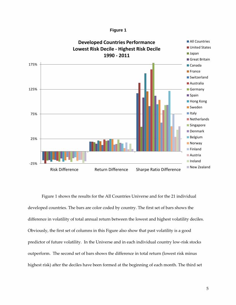
Figure 1

Figure 1 shows the results for the All Countries Universe and for the 21 individual

developed countries. The bars are color coded by country. The first set of bars shows the

difference in volatility of total annual return between the lowest and highest volatility deciles.

Obviously, the first set of columns in this Figure also show that past volatility is a good

predictor of future volatility. In the Universe and in each individual country low-risk stocks

outperform. The second set of bars shows the difference in total return (lowest risk minus

highest risk) after the deciles have been formed at the beginning of each month. The third set

-25%

25%

75%

125%

175%

Risk Difference Return Difference Sharpe Ratio Difference

Developed Countries Performance Lowest Risk Decile - Highest Risk Decile

1990 - 2011

All Countries

United States

Japan

Great Britain

Canada

France

Switzerland

Australia

Germany

Spain

Hong Kong

Sweden

Italy

Netherlands

Singapore

Denmark

Belgium

Norway

Finland

Austria

Ireland

New Zealand

6

shows the difference in the Sharpe ratios (average return to volatility)8 between the lowest

volatility decile and the highest. The results are even more dramatic on a risk-adjusted basis.

For the U.S. the turnover in the deciles averages 84% per year; for the All Countries Universe it

is 96% per year.

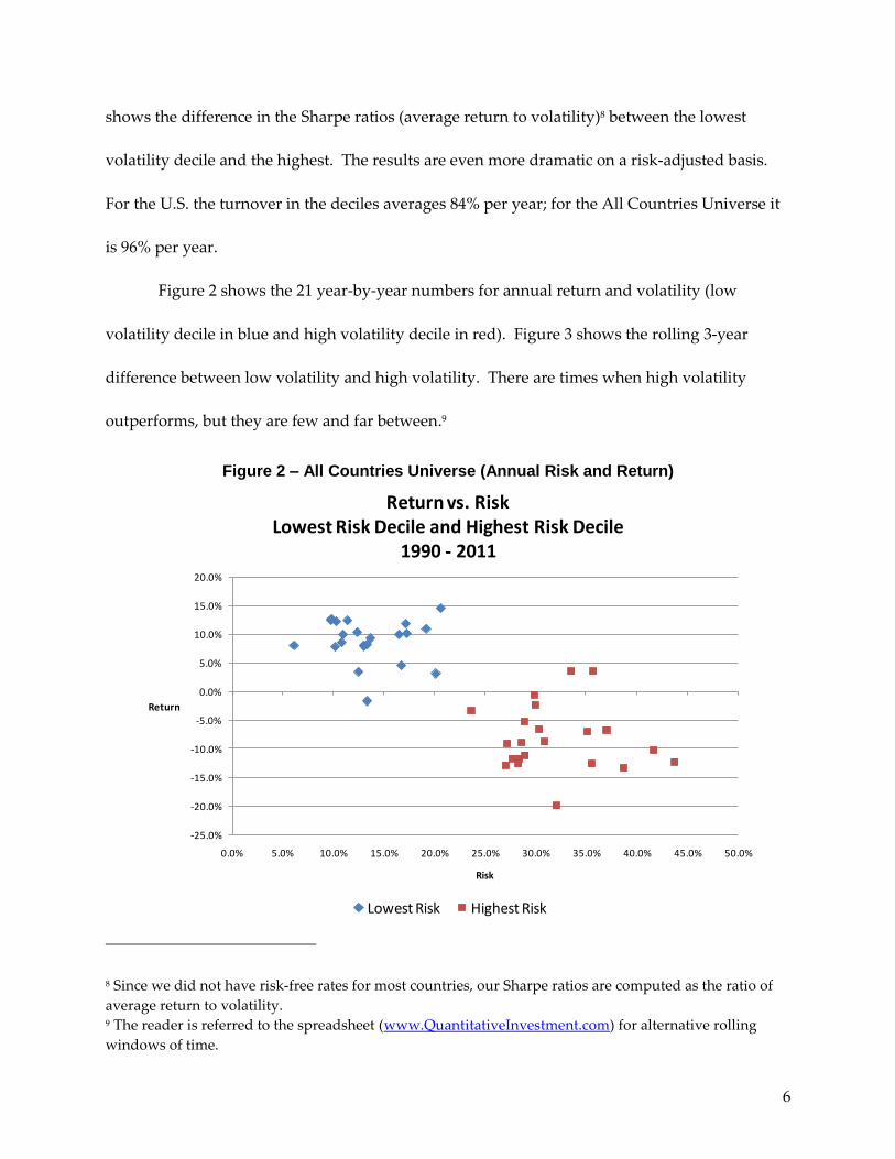
Figure 2 shows the 21 year-by-year numbers for annual return and volatility (low

volatility decile in blue and high volatility decile in red). Figure 3 shows the rolling 3-year

difference between low volatility and high volatility. There are times when high volatility

outperforms, but they are few and far between.9

Figure 2 – All Countries Universe (Annual Risk and Return)

8 Since we did not have risk-free rates for most countries, our Sharpe ratios are computed as the ratio of

average return to volatility. 9 The reader is referred to the spreadsheet (www.QuantitativeInvestment.com) for alternative rolling

windows of time.

-25.0%

-20.0%

-15.0%

-10.0%

-5.0%

0.0%

5.0%

10.0%

15.0%

20.0%

0.0% 5.0% 10.0% 15.0% 20.0% 25.0% 30.0% 35.0% 40.0% 45.0% 50.0%

Return

Risk

Return vs. Risk Lowest Risk Decile and Highest Risk Decile

1990 - 2011

Lowest Risk Highest Risk

7

Figure 3

Figure 4

-25%

25%

75%

125%

175%

Risk Difference Return Difference Sharpe Ratio Difference

Emerging Markets Performance Lowest Risk Decile - Highest Risk Decile

1990 - 2011 All Emerging

China

Korea

Brazil

Taiwan

South Africa

India

Indonesia

Thailand

Chile

Poland

Israel

Philippines

-20%

-10%

0%

10%

20%

30%

40%

50%

60%Rolling 3-year

Difference in Return

Lowest Risk Decile - Highest Risk Decile All Countries

8

In Figure 4 we show our results for emerging markets. Identical procedures were used

to construct Figure 4 as for Figure 1.10

Why Do Risky Stocks Sell at Premium Prices?

Some researchers don’t believe that risky stocks do sell at premium prices. They explain

away the anomalies they encounter by using statistical procedures. In the case of Fama-French

(1992), they risk-adjusted the return to value and growth stocks by regressing three factors: (a)

the risk premiums on these stocks against the risk premiums on the market, (b) the difference in

the returns for large stocks and small stocks and (c) the difference in returns between value and

growth stocks. They then focus on the intercept of this regression as a measure of risk-adjusted

return.

However, this methodology is questionable. Essentially, the Fama-French intercept is

the expected difference in return between value and growth under market conditions where:

(a) the market produces a return equal to the risk-free rate, (b) big stocks do not outperform

small stocks and (c) value stocks do not outperform growth stocks. In this market environment,

of course, you would predict the conditional expected return to value and growth to be the

same.

Carhart (1997) has taken this procedure a step further in order to explain a fourth factor,

the momentum anomaly. This anomaly contends that stocks that have done well in the trailing

10 Blitz, Pang and van Vliet (2012) have found similar results for emerging markets. Mexico and Russia

were not included in our results because of an insufficient number of stocks in each market. Mexico did

not have 100 stocks in our database until the end of 2006. Russia did not have 100 stocks until the end of

2008.

9

intermediate term (six months to a year) will tend to outperform in the future. Carhart adds

this momentum anomaly to explain the difference in future returns of high and low trailing

momentum stocks. Using this expanded “risk-adjustment” technique, he finds that under

conditions when the realized performances of high and low momentum stocks are equal, high

momentum stocks shouldn’t be expected to outperform low momentum stocks. (Yes, you read

that correctly.)

In similar fashion, some finance researchers cast the low volatility anomaly aside by

adding a fifth factor that is the difference in return between high volatility stocks and low

volatility stocks. Using this technique, Scherer (2011) has found that there is no difference in the

expected returns to low and high volatility stocks in market environments where high and low

volatility stocks can be expected to perform equally.

However we believe that all this statistical maneuvering blinds researchers not only to

the existence of the anomaly, but also to the possible real explanations of it.

Perhaps the nature of the third moment (skewness) of the distributions for returns can

explain the negative relationships between the first two moments (expected return and

variance). The suggestion that investors have a preference for positive skewness is reasonable.

However, investors seek to diversify and there is no evidence that well-diversified equity

portfolios can be constructed with a degree of skewness sufficient to overcome the lower

expected returns on high volatility portfolios.

Brennan (1992) suggests that limits to arbitrage may create a security market line that is

flatter than predicted by the CAPM. Managers who are directed to maximize the information

ratio (their alpha divided by their tracking error) may look at two stocks, the first with a beta

10

less than one and the second with a beta greater than one, as equally risky. Even if the low beta

stock has a positive alpha and would reduce the managers’ Sharpe ratios it may actually

increase their information ratios. Therefore, these managers may not reach for low beta stocks

with positive alphas resulting in a flattening of the security market line in an equilibrium

setting. However, this justification cannot explain the inverted relationship between risk and

return that is obvious in the data.

We submit that the anomaly can be explained by the nature of manager compensation

and agency issues (a) between professional investment managers within an organization and (b)

between these professionals and their clients.11

11 In the early years of the Haugen Heins study, institutional investment was far less important than it is

today. However, to a great extent, the individual investors as well as the less important institutions

relied on investment advisors who were subject to the same agency issues discussed below.

11

Figure 5

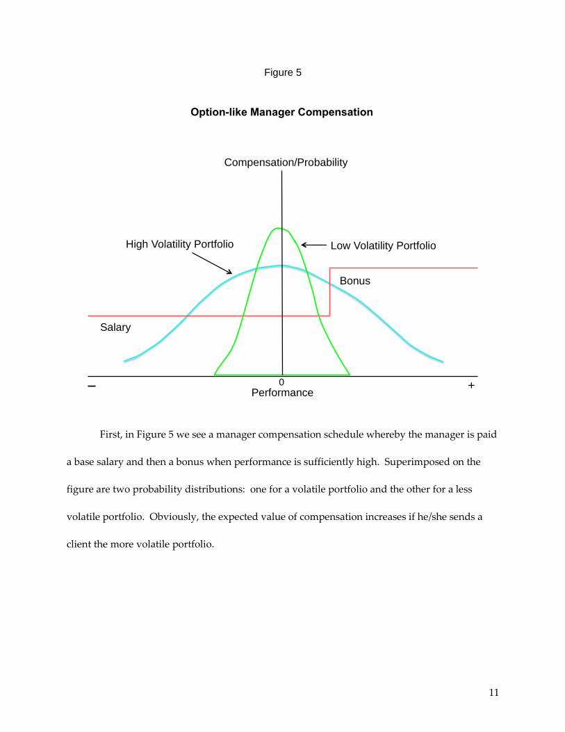
First, in Figure 5 we see a manager compensation schedule whereby the manager is paid

a base salary and then a bonus when performance is sufficiently high. Superimposed on the

figure are two probability distributions: one for a volatile portfolio and the other for a less

volatile portfolio. Obviously, the expected value of compensation increases if he/she sends a

client the more volatile portfolio.

Option-like Manager Compensation

High Volatility Portfolio Low Volatility Portfolio

Salary

Bonus

Performance 0 +

Compensation/Probability

12

Second, a significant issue exists amongst the investment managers themselves that

creates excess demand for more volatile stocks12. Periodic investment committee meetings are

central to the process of building a model portfolio. This model portfolio serves as a guide for

the construction of individual portfolios for clients.

Typically at these meetings, a team of analysts, each individually specializing in a

particular industry or sector, sits before the Chief Investment Officer (CIO). Each in turn, the

analysts are asked to make a case for stocks they believe should be included in the model

portfolio. Naturally, these analysts want to impress the CIO and their fellow analysts with their

prowess in selecting meritorious investments. Failing to make their case time after time could

result in stagnation or even termination, rather than advancement.

Consequently, they are attracted to stocks for which they can confidently make a

compelling case. These stocks tend to be noteworthy, often by virtue of receiving media

attention. Because the flow of new information about these stocks is relatively intense, stocks of

this type tend to exhibit higher than average volatility. Therefore, based on the analysts’

desires to impress their colleagues, we would expect that stocks with higher than average

volatility would tend to be included in the model portfolio.

In addition, the interesting nature of these stocks makes it easier for professional money

managers to explain changes in the model portfolio to their clients. Most professional money

managers are not quantitative. For many, a standard deviation is a long ago memory from their

12 Baker, Bradley and Wurgler (2011) argue that individuals themselves might have a preference for

volatile stocks. See pages 44-45 of their Financial Analysts Journal article.

13

college statistics class. These managers may realize that the stocks they are recommending are

newsworthy, but the fact that they are also more volatile may escape their attention.

Consequently, these agency issues create demand by professional investors and their

clients for highly volatile stocks. This demand overvalues the prices of volatile stocks and

suppresses their future expected returns.

This being the case, we would expect that institutional investors tend to hold more

volatile stocks. To determine whether this is true, we look at roughly the largest 1000 stocks in

the United States in the time period 2000 through 2009. Again, volatility is calculated using a

24-month trailing window. The percentage of a stock’s total market capitalization held by

institutional investors is obtained from the Thomson Reuters database.

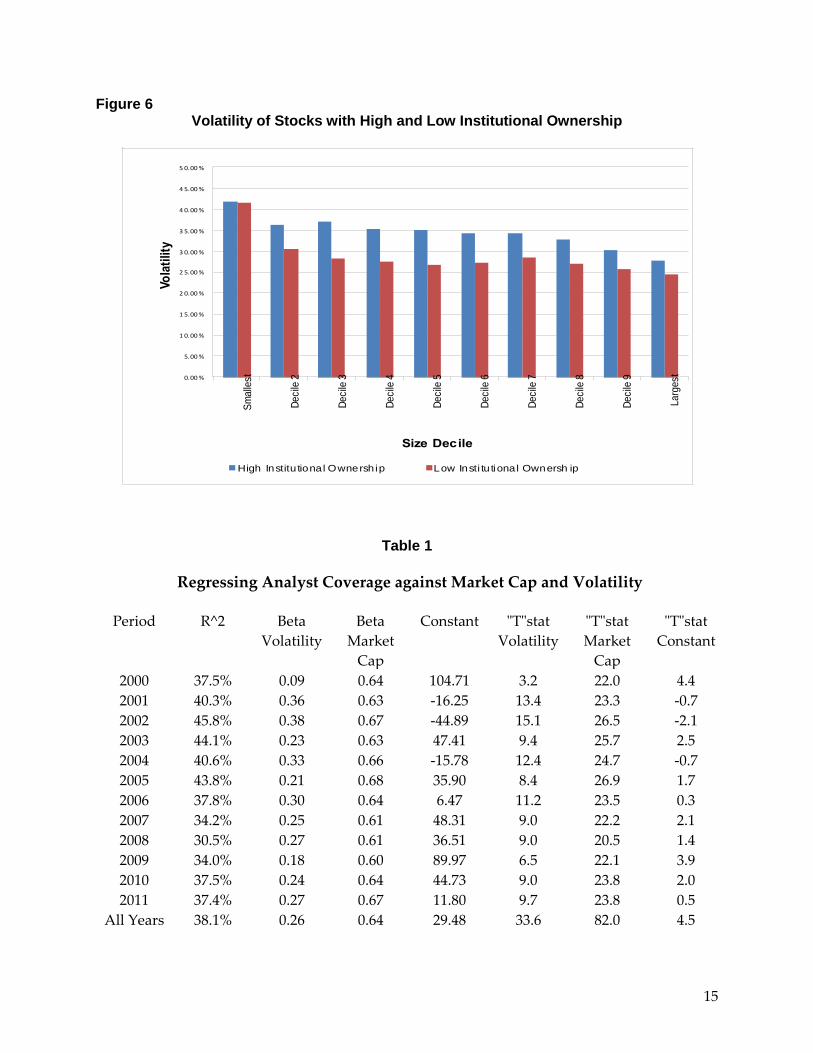
First we form size deciles based on market capitalization. Then, within each size decile,

we form three equally populated groups based on the percentage of stock held by institutions.

In Figure 6 we focus on the high and the low institutional ownership groupings. The table

reveals that except for the very smallest stocks, institutions do indeed hold more volatile

stocks.13

In Table 1 we provide evidence that the intensity of analysts’ coverage is significantly

greater for more volatile stocks. The study covers roughly the largest 1000 U.S. stocks. The

13 In an earlier study that provides the basis for our methodology, Sias (1996) finds very similar results for

a previous period. We note that Sias has a competing explanation for the results. He contends that

institutions induce volatility via price pressure coming from their trading activity. We contend they hold

more volatile stocks because of the agency problems discussed above. Under the Sias hypothesis, we

would expect to see the difference in volatility become greater with the smaller capitalization stocks. In

fact his results and ours show the opposite pattern. Therefore we conclude that both results are more

likely the product of agency issues rather than the market impacts of trading. We note that the market

impact hypothesis and our agency hypothesis are not mutually exclusive. Both may explain why

institutions hold more volatile stocks.

14

time period extends only from 2000 to 2011 due to data limitations. In each year we run a cross

sectional regression where the dependent variable is the rank14 of each stock (from 1 to 1000)

based on the number of analysts providing a buy, sell or hold recommendation for each stock.

The independent variables are each stock’s rank in terms of market capitalization and its

trailing volatility over the proceeding 360 trading days. We find that more volatile stocks do

attract more analysts’ coverage. The “T” statistics in each year are highly significant and even

more so for the overall period.

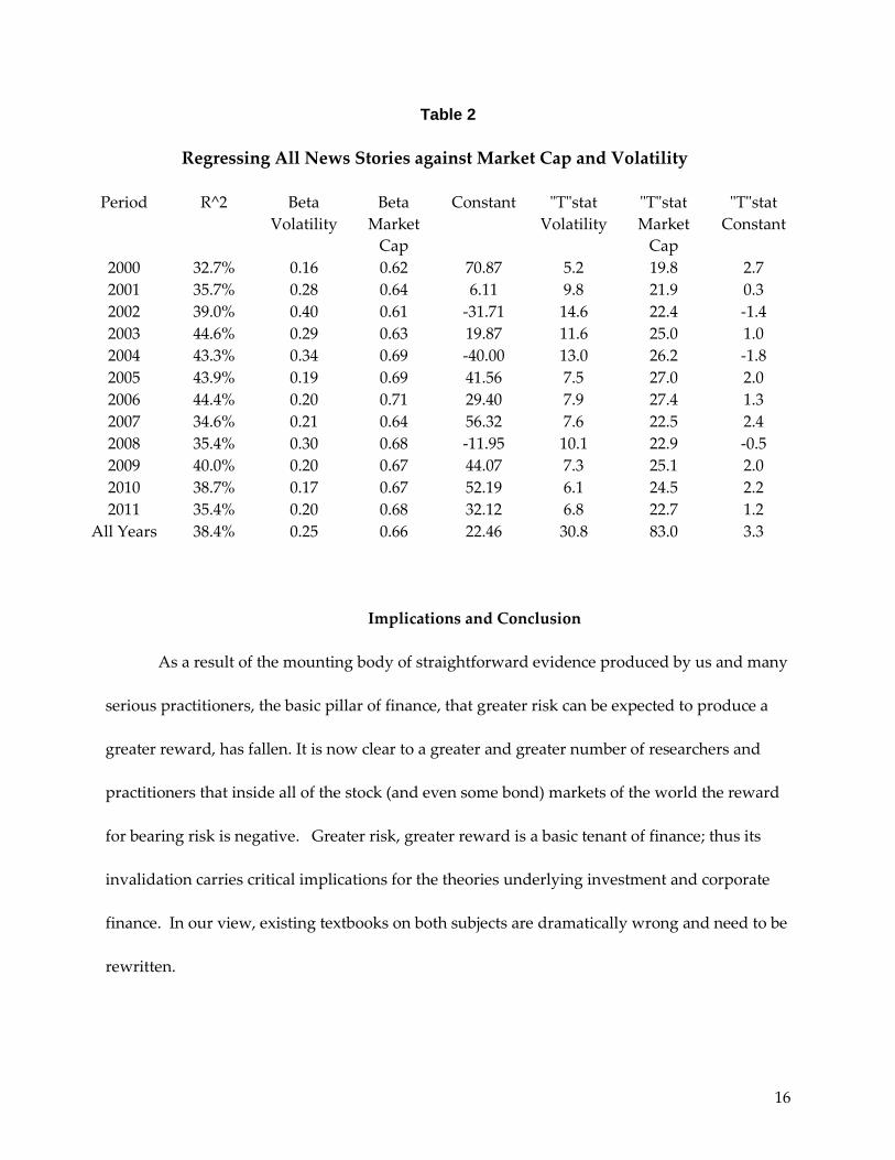
In Table 2 we provide evidence relating to the relationship between volatility and news

coverage. Here we run the same regressions as in Table 1, but the dependent variable is the

number of stories appearing on the Dow Jones News Wire for each stock15. The number of

stories ranges from 7,220 in the first year to 17,778 in the last. We see that volatile stocks are, in

fact, covered more intensely by the media. Once again all the statistics are highly significant.16

Thus we find that (a) financial institutions hold more volatile stocks, (b) analysts’

coverage is significantly greater for more volatile stocks, and (c) news coverage is more intense

for more volatile stocks. All the evidence is consistent with our hypothesis that agency issues

are responsible for creating demand for volatile stocks, which results in their over-pricing and

their production of inferior returns in the future. 17

14 We use rankings in order to normalize the data. 15 We thank RavenPack for providing us with data on news stories. 16 Consistent with our agency hypothesis, the cross-sectional correlation between coverage and news is

49%. 17 Interestingly, the inability of managers to outperform has always been the strongest piece of evidence

for proponents who believe that the market is efficient. The evidence provided in this paper is consistent

with a highly inefficient market. So why can’t the analysts beat it? They are the victims of their own

investment process.

15

Figure 6 Volatility of Stocks with High and Low Institutional Ownership

Table 1

Regressing Analyst Coverage against Market Cap and Volatility

Period R^2 Beta

Volatility

Beta

Market

Cap

Constant "T"stat

Volatility

"T"stat

Market

Cap

"T"stat

Constant

2000 37.5% 0.09 0.64 104.71 3.2 22.0 4.4

2001 40.3% 0.36 0.63 -16.25 13.4 23.3 -0.7

2002 45.8% 0.38 0.67 -44.89 15.1 26.5 -2.1

2003 44.1% 0.23 0.63 47.41 9.4 25.7 2.5

2004 40.6% 0.33 0.66 -15.78 12.4 24.7 -0.7

2005 43.8% 0.21 0.68 35.90 8.4 26.9 1.7

2006 37.8% 0.30 0.64 6.47 11.2 23.5 0.3

2007 34.2% 0.25 0.61 48.31 9.0 22.2 2.1

2008 30.5% 0.27 0.61 36.51 9.0 20.5 1.4

2009 34.0% 0.18 0.60 89.97 6.5 22.1 3.9

2010 37.5% 0.24 0.64 44.73 9.0 23.8 2.0

2011 37.4% 0.27 0.67 11.80 9.7 23.8 0.5

All Years 38.1% 0.26 0.64 29.48 33.6 82.0 4.5

0.00%

5.00%

1 0.00%

1 5.00%

2 0.00%

2 5.00%

3 0.00%

3 5.00%

4 0.00%

4 5.00%

5 0.00%

Sm

alle

st

De

cile

2

De

cile

3

De

cile

4

De

cile

5

De

cile

6

De

cile

7

De

cile

8

De

cile

9

La

rges

t

Vo

lati

lity

Size Decile

High Institu tional Ownersh ip Low Insti tu tional Ownersh ip

16

Table 2

Regressing All News Stories against Market Cap and Volatility

Period R^2 Beta

Volatility

Beta

Market

Cap

Constant "T"stat

Volatility

"T"stat

Market

Cap

"T"stat

Constant

2000 32.7% 0.16 0.62 70.87 5.2 19.8 2.7

2001 35.7% 0.28 0.64 6.11 9.8 21.9 0.3

2002 39.0% 0.40 0.61 -31.71 14.6 22.4 -1.4

2003 44.6% 0.29 0.63 19.87 11.6 25.0 1.0

2004 43.3% 0.34 0.69 -40.00 13.0 26.2 -1.8

2005 43.9% 0.19 0.69 41.56 7.5 27.0 2.0

2006 44.4% 0.20 0.71 29.40 7.9 27.4 1.3

2007 34.6% 0.21 0.64 56.32 7.6 22.5 2.4

2008 35.4% 0.30 0.68 -11.95 10.1 22.9 -0.5

2009 40.0% 0.20 0.67 44.07 7.3 25.1 2.0

2010 38.7% 0.17 0.67 52.19 6.1 24.5 2.2

2011 35.4% 0.20 0.68 32.12 6.8 22.7 1.2

All Years 38.4% 0.25 0.66 22.46 30.8 83.0 3.3

Implications and Conclusion

As a result of the mounting body of straightforward evidence produced by us and many

serious practitioners, the basic pillar of finance, that greater risk can be expected to produce a

greater reward, has fallen. It is now clear to a greater and greater number of researchers and

practitioners that inside all of the stock (and even some bond) markets of the world the reward

for bearing risk is negative. Greater risk, greater reward is a basic tenant of finance; thus its

invalidation carries critical implications for the theories underlying investment and corporate

finance. In our view, existing textbooks on both subjects are dramatically wrong and need to be

rewritten.

17

In terms of the investment theory, it is clear that the directive to invest in capitalization-

weighted portfolios as a core strategy is ill-advised. The performance of these portfolios is

dominated by the presence of relatively volatile and over-valued growth stocks. The inflated

prices of growth stocks reflect the market’s expectation that their relative profitability won’t be

eroded in the future by the entrance of competition. In addition, text books need to return to

teaching students the basic tools required for stock investing – such as standardizing accounting

numbers to reflect different measurement standards over different industries and sectors.

Students may also want to study the cross-predictability across a company’s suppliers,

customers and competitors. They should understand that there are a myriad of determinants of

expected stock return. Beta may be one of them, but it is relatively weak, and it typically has the

wrong sign.18

In addition, most of the propositions set forth in corporate finance text books are based

on the concept of efficient financial markets. For example the theories of Modigliani and Miller

(1958) suggest that the firm should be indifferent to financing with debt, equity or anything else

in an efficient market where all securities are fairly priced.

In an inefficient market financiers should behave very differently. Instead of following

their finance textbooks, management should operate in the following investment and financing

decision framework:

In considering the costs of raising internal capital, managers should employ state-of-the-

art inductive technology (supplemented with their own information) to forecast the expected

18 See Haugen and Baker (2006).

18

returns to their firm’s menu of prospective securities and portfolios of their securities. Forecasts

of the expected returns to these securities, and portfolios of securities, should be based on

statistical models that explain and forecast the behavior of stock market prices.

In financing, managers should determine the least-expensive portfolio of securities that

can be issued. As long as the firm’s assets are over or undervalued by the market, management

should be able to create financing portfolios that are overvalued. In finding the least-expensive

portfolio to finance, it matters not what the firm’s security holders expect the returns to be or

even what they want them to be. What counts is what management believes they are going to

be.

Next, management should consider its investment alternatives both in the real sector

and in the financial sector. Remember, in the inefficient market, armed with state-of-the-art

expected return statistical models, management may see investments with very high rates of

return in the financial markets. Management’s own stock may be one of these, but it is special

only in the context of management’s private information and the fact that it is a tax-free

investment. These financial expected returns should be compared with alternatives in the real

sector.

In a tax-free world, assuming away attendant problems associated with mutually

exclusive investments, issues of signaling, agency problems, and other factors that create

interdependence between the investment and a financing decision, management should opt for

the investment with the highest risk-adjusted expected return, provided the returns are higher

than the expected returns on the lowest-cost bundle of securities used to finance. Management

19

should continue its external financing and investing until the gap between the risk-adjusted

expected returns to its investments and the lowest-cost source of finance closes.

For investments internally financed, management should accept projects that have

expected returns greater than required by its stockholders. Following these paths, expected

stockholder wealth is maximized.

You may now ask: how can it be true that over the course of almost fifty years, millions

of unsuspecting students have been trained by thousands of finance professors to believe in the

tenants of efficient markets? The answer is that in all but the hardest of sciences, academic

research may be influenced by other factors in addition to a pure quest for the truth. Academics

are human beings and subject to the influences and tendencies of all humans. Thus, in some

cases, research may be influenced by the desire to obtain or preserve power and recognition.

Once power and influence are acquired, say by the publication of a revolutionary idea, it is

clearly in the interest of the author to preserve that power and influence.

In academia, power can be preserved through the students of the author. Based on high

regard for the revolutionary idea and its creator, these students are hired by prestige

universities and become referees and associate editors of the best journals. It is human nature

to favor evidence that is consistent with your training and beliefs. Whether consciously or

unconsciously, the net result is that evidence that is inconsistent with the dominant paradigm is

suppressed and the power and reward associated with supporting the status quo is escalated.

Eventually, associate editors are promoted to editors of the premier journals. Success in

academics is, to a great extent, determined by publishing in these journals.

20

Now graduate students in finance all over the world are trained in highly complex

mathematical modeling. Most of these models are elegant and highly sophisticated, and the

work is highly challenging. Evidence that renders their sophisticated training impotent in

terms of predicting and explaining behaviors in financial markets will be viewed with extreme

disdain. If they accept conflicting evidence, these economists confront the prospect of their own

obsolescence. They have a vested interest in favoring evidence consistent with their own beliefs

and rejecting evidence to the contrary.

For those who produce research results that discredit the dominant paradigm, the road

to academic success and professional recognition can be difficult. Over the years, we have met

several individuals who had academic careers terminated by their inability to get their own

discovery of what we found in 1972 published.

In our opinion, we are now in the midst of a second paradigm shift in the field of

finance. This time the shift is being driven by the research of practitioners rather than

academics, whose self-interest is firmly tied to defending the current paradigm. These

practitioners should begin hiring finance graduates who are properly trained in solving

problems in real as opposed to imaginary markets.

21

Bibliography

Ang, Andrew, Robert J. Hodrick, Yuhang Xing and Xiaoyan Zhang (2006), “The Cross Section of

Volatility and Expected Returns,” Journal of Finance, February 2006, pp. 259-299.

Ang, Andrew, Robert J. Hodrick, Yuhang Xing and Xiaoyan Zhang (2009), “High Idiosyncratic

Volatility and Low Returns: International and Further U.S. Evidence," Journal of Financial

Economics, pp. 1-23.

Arnott, Robert (1983), “What Hath MPT Wrought: Which Risks Reap Rewards?” The Journal of

Portfolio Management, Fall 1983, pp. 5-11.

Blitz, David C. (2011), “Strategic Allocation to Premiums in the Equity Market,” SSRN Working

Paper no. 1949008, Journal of Index Investing, pp. 42-49.

Blitz, David, Juan Pang, and Pim van Vliet (2012), "The Volatility Effect in Emerging Markets,”

Robeco Research paper, April 2012.

Blitz, David C. and Pim van Vliet (2007), “The Volatility Effect: Lower Risk without Lower

Return,” Journal of Portfolio Management, pp. 102–113.

Carhart, Mark M. (1997), "On Persistence in Mutual Fund Performance," Journal of Finance, pp.

57–82.

Haugen, Robert A. and A. James Heins (1972), “On the Evidence Supporting the Existence of

Risk Premiums in the Capital Markets,” Wisconsin Working Paper, December 1972.

Haugen, Robert A. and A. James Heins (1975), “Risk and the Rate of Return on Financial Assets:

Some Old Wine in New Bottles,” Journal of Financial and Quantitative Analysis, pp.775–784.

Haugen, Robert A. and Nardin L. Baker (1991), “The Efficient Market Inefficiency of

Capitalization-Weighted Stock Portfolios,” The Journal of Portfolio Management, pp. 35-40.

Haugen, Robert A. and Nardin L. Baker (1996), “Commonality in the Determinants of Expected

Stock Returns,” Journal of Financial Economics, 401–439.

22

Haugen, Robert A. and Nardin L. Baker (2010), “Case Closed,” The Handbook of Portfolio

Construction: Contemporary Applications of Markowitz Techniques, Edited by John B. Guerard Jr.

(Springer-Verlag US), Chapter 23. See also http://ssrn.com/abstract=1306523.

Jagannathan R. and T. Ma (2003), “Risk Reduction in Large Portfolios: Why Imposing the

Wrong Constrains Helps,” The Journal of Finance, pp. 1651-1684.

Jensen, Michael C. (1969), "Risk, the Pricing of Capital Assets and the Evaluation of Investment

and Portfolios," The Journal of Business, pp. 167-247.

Leote de Carvalho, Raul, Xiao Lu and Pierre Moulin (2011), “Demystifying Equity Risk-Based

Strategies: A Simple Alpha plus Beta Description,” The Journal of Portfolio Management, pp. 56-70.

See also papers.ssrn.com/sol3/papers.cfm?abstract_id=1949003

Modigliani, F. and Miller, M. (1958), "The Cost of Capital, Corporation Finance and the Theory

of Investment," American Economic Review, pp. 261–297.

Scherer, Bernd (2011), “A Note on the Returns from Minimum Variance Investing,” Journal of

Empirical Finance, pp. 652-660.

Sharpe, William F. (1964), "Capital Asset Prices: A Theory of Market Equilibrium under

Conditions of Risk," The Journal of Finance, pp. 425-442.

Sias, Richard (1996), “Volatility and the Institutional Investor,” Financial Analysts Journal, Vol.

52, No. 2, pp. 13-21.

Soldofsky, Robert M. and Roger L. Miller (1969), "Risk Premium Curves for Different Classes of

Long-Term Securities, 1950-1966," The Journal of Finance, pp. 429-445.