low power task scheduling and mapping for applications ... · the scheduling software to assist...

Copyright © 2012 American Scientific PublishersAll rights reservedPrinted in the United States of America

Journal ofLow Power Electronics

Vol. 8, 1–16, 2012

Low Power Task Scheduling and Mapping forApplications with Conditional Branches onHeterogeneous Multi-Processor System

Yang Ge1�∗, Yukan Zhang1, Parth Malani2, Qing Wu3, and Qinru Qiu11Department of Electrical Engineering and Computer Science, Syracuse University, Syracuse, NY, 13210, USA

2Intel Corporation, Santa Clara, CA, 95054, USA3Air Force Research Laboratory, Rome, NY, 13441, USA

Many real time applications demonstrate uncertain workload that varies during runtime. One of themajor influences of the workload fluctuation is the selection of conditional branches which activateor deactivate a set of instructions belonging to a task. In this work, we capture the workload dynam-ics using Conditional Task Graph (CTG) and propose a set of algorithms for the optimization of taskmapping, task ordering and dynamic voltage/frequency scaling of CTGs running on a heteroge-neous multi-core system. Our mapping algorithm balances the latency and the energy dissipationamong heterogeneous cores in order to maximize the slack time without significant energy increase.Our scheduling algorithm considers the statistical information of the workload to minimize the meanpower consumption of the application while maintaining a hard deadline constraint. The proposedDVFS algorithm has pseudo linear complexity and achieves comparable energy reduction as thesolutions found by mathematical programming. Due to its capability of slack reclaiming, our DVFStechnique is less sensitive to the slight change in hardware or workload and works more robustlythan the conventional DVFS techniques.

Keywords: Dynamic Voltage and Frequency Scaling, Multiprocessor System-on-Chip, ProcessorScheduling, Workload Variation.

1. INTRODUCTION

The Multiprocessor System-on-Chip (MPSoC) has becomea major system design platform for general purpose andreal-time applications, due to its low design cost and highperformance. Power consumption, which has already beena roadblock for current single core systems, will continueto be a major design concern for MPSoC. There have beencontinuous design efforts targeting at energy reduction ofMPSoC. Dynamic Voltage and Frequency Scaling (DVFS),which allows the processor to dynamically alter its speedand voltage at run time, is one of the most popular energyreduction techniques at system level.Many techniques have been proposed that perform

power aware task mapping, ordering and DVFS for appli-cations with fixed workload.1∼3 However, they may notachieve their best performance with real life applicationsthat demonstrate workload variations.This paper considers task scheduling and voltage

selection of applications with variable workload on a

∗Author to whom correspondence should be addressed.Email: [email protected]

heterogeneous multiprocessor system-on-chip. We focuson the set of applications which can be decomposed intorepeated tasks with relatively constant execution time. Theuncertainty of the workload is reflected by the randomactivation and deactivation of certain tasks during run-time and it is captured by branch selections among tasks.We assume that such branch information is observable tothe scheduling software to assist runtime scheduling andpower management of the system. Examples of such tasklevel branching include branches that enable or disableIDCT function during MPEG decoding or branches thatselect different modulation schemes for preamble and pay-load based on 802.11b physical layer standard. We modelan application with dynamic branch selections using a con-ditional task graph (CTG).4∼8

Although instruction level branch prediction is a com-mon practice in high performance processors, the predic-tion is not perfect. The task graphs that we are workingwith are high level abstraction of large applications. Theselection of conditional branches depends mostly on theinput data, which are random variables. This makes accu-rate branch prediction even more difficult. Techniques that

J. Low Power Electron. 2012, Vol. 8, No. 5 1546-1998/2012/8/001/016 doi:10.1166/jolpe.2012.1214 1

Low Power Task Scheduling and Mapping for Applications with Conditional Branches Ge et al.

dynamically assign confidence levels9 or probabilities10 tothe conditional branches have been proposed by previousresearch works. For many applications, the branch prob-ability exhibits strong temporal correlations and can bepredicted based on history. Such information will be usedby the proposed scheduling algorithm for expected energyminimization.We study the power aware task mapping and schedul-

ing techniques for the CTGs with a particular interest intheir performance on the heterogeneous multi-core system.It is important to investigate the low power techniques forthe heterogeneous multi-core system, not only because itis the architecture of many embedded computing systemssuch as the Pasta sensor node,15 the LEAP system,16 andthe mPlatform,17 but also because, due to the within-dievariation and transistor wear-out, a homogenous multi-coresystem will exhibit heterogeneity over time.18

The proposed framework optimizes the task mapping,task ordering and dynamic voltage/frequency scaling ofCTGs running on a heterogeneous multi-core system. Dueto the probabilistic branching, the execution of CTG is arandom process. Our goal is to minimize the mean powerconsumption instead of the worst case power consump-tion of the application while meeting the hard real-timeconstraint. Our mapping algorithm balances the latencyand the energy dissipation among heterogeneous coresin order to maximize the slack time without signifi-cant energy increase. Our scheduling algorithm minimizesthe mean power consumption of the application whilemaintaining a hard deadline constraint. Our DVFS algo-rithm dynamically distributes slacks during runtime, andachieves comparable energy reduction as the solutionsfound by non-linear mathematical programming. Due to itscapability of slack reclaiming, our DVFS technique is lesssensitive to the slight change in hardware or task execu-tion and works more robustly than the conventional DVFStechniques. Please note that to minimize the power con-sumption of an application with hard real-time constraintis equivalent to minimize the energy consumption, becausethe energy is the product of power and execution time.To the best of our knowledge, this is the first paper

that addresses low power scheduling of conditional taskgraphs on heterogeneous multi-core platform. Comparedto the existing works, the uniqueness of our approach canbe summarized as the following.The proposed framework optimizes task mapping and

scheduling simultaneously. We modify the Dynamic Levelbased Scheduling (DLS) algorithm11 to find mapping andscheduling of CTGs on a heterogeneous platform. Thecomplexity of task mapping and ordering is O�MN�where M is the number of processing elements (PEs) inthe system and N is the number of tasks in the taskgraph.We consider the application with conditional execu-

tion as a random procedure in which the branch selectionprobabilities can be profiled (or measured). Our algorithm

utilizes such statistical information in each optimizationstep to reduce the mean power consumption.The proposed slack reclaiming based DVFS algorithm

has pseudo-linear complexity with the respect to the num-ber of tasks in the CTG. It also performs more robustly thanthe DVFS solution found by mathematical programming.More generalized hardware and software models are

targeted in this work. The hardware platform consists ofheterogeneous processing elements with different power-performance tradeoff characteristics. The only assumptionthat is required by our DVFS algorithm is a convex relationbetween the power and performance for each PE, whichis usually true for many devices. The software applicationconsists of a set of tasks with data and control dependen-cies and hard deadline constraint.The rest of the paper is organized as follows: Section 2

introduces the existing works in related area. Section 3introduces the application and hardware architecture mod-els; Sections 4 and 5 present in detail the underlyingscheduling, mapping and DVFS algorithms. Section 6gives the experimental results. Finally, Section 7 concludesthe paper.

2. RELATED WORKS

Task mapping, ordering, and DVFS for CTGs have beenstudied in many literatures. In Ref. [4], Dolif et al. pro-pose an exact analytic formulation of the stochastic objec-tive function for conditional task mapping and schedulingbased on task graph analysis. Their approach considersstochastic branching probabilities and improves the over-all performance by optimizing the bus activity. In Ref. [5],Eles et al. present an approach to minimize the worstcase delay, which considers the communication workloadand branch control. A recursive algorithm is proposed togenerate the schedule table, which stores the start timeof each task at different execution scenarios. In Ref. [6],Xie et al. propose a task mapping and scheduling algo-rithm which is sensitive to mutually exclusive tasks inthe CTG. Their algorithm exploits the processor sharingfor mutually exclusive tasks to minimize the worst casedelay of the CTG. All these works do not minimize energydissipations.Wu et al.7 utilize a scheduling table for runtime DVFS.

The slack time of each task can be derived from the table.A genetic algorithm based task mapping algorithm is pro-posed for further energy savings. An implicit assumptionof this technique is that all the conditional branches will beselected with equal probability, which might not be realis-tic for a real system. Furthermore, the GA based task map-ping algorithm has very high complexity because the innerloop of this algorithm needs to perform the task orderingand stretching for the entire CTG.Shin et al.8 proposed an algorithm for task scheduling

and DVFS of CTG which considers the run-time behavior.The algorithm is based on a modified list scheduling and

2 J. Low Power Electron. 8, 1–16, 2012

Ge et al. Low Power Task Scheduling and Mapping for Applications with Conditional Branches

non-linear programming (NLP) based voltage/frequencyoptimization. Because the algorithm schedules a task withdifferent start time and speed under different branch selec-tion scenarios, it is referred as condition aware scheduling.However, their task mapping is assumed to be fixed.In Refs. [13 and 14] we proposed a Communica-

tion Aware Probability-based (CAP) scheduling algorithmsfor CTGs on a DVFS enabled multiprocessor platform.However, the algorithm assumes that all the PEs havethe same energy-performance characteristics. Furthermore,its DVFS algorithm relies on evaluating all the paths,which has exponential complexity. In this paper, wecompletely revised the CAP algorithm and consider aheterogeneous system where each PE has unique power-performance characteristics. The complexity of the DVFSalgorithm is also significantly reduced.Power aware task mapping, scheduling and DVFS tech-

niques for heterogeneous multiprocessor system has beenstudied in Refs. [19∼25]. In Ref. [19], a two-phasealgorithm is proposed for distributed real-time embeddedsystem. A static scheduling algorithm first generates theschedule for all tasks in the CTG, and then a dynamicscheduling algorithm determines the speed ratio for mutualexclusive tasks during the runtime. In Ref. [20], the authorsfocus on the critical paths and distribute the slack timeover the tasks on the critical path to achieve energy sav-ings. Both works assume that only processors have DVFScapability and their power-performance characteristics areidentical. References [21 and 22] study the energy-efficientsoftware partition in heterogeneous multiprocessor sys-tem. In Ref. [21], Goraczko et al. formulate the softwarepartitioning problem as an integer linear programming(ILP) constrained by the deadline. The solution of theILP gives the number of processors needed by the sys-tem and task mapping information. In Ref. [22], Yanget al. present an approximate algorithm for task partition tofind near-optimal task mapping and scheduling with min-imum energy consumption. In both these works, tasks areassumed to be independent to each other. A leakage awareDVFS algorithm is proposed in Ref. [23]. Unlike our work,it only considers heterogeneous system with only 2 typesof processing elements (PE), one with high performanceand high power consumption while the other with lowperformance and low power consumption. The objectiveis to maximize the number of tasks mapped on the PEswith low performance while satisfy the deadline constraint.Deadline Monotonic (DM) rule is used in the task schedul-ing while Random Algorithm (RA), First-Fit DecreasingDensity (FFDD), Genetic Algorithm (GA) and SimulatedAnnealing (SA) are used for task mapping. In Ref. [24],Azevedo et al. propose to do intra task DVS based on theprogram checkpoint, while in Ref. [25], Yang et al. relythe Pareto curve profiling for a task graph to do onlinetask mapping and scheduling. Both of these works do notconsider energy and performance heterogeneity of the mul-tiprocessor platform.

3. APPLICATION AND ARCHITECTUREMODELING

The CTG that we are using is similar to the one specifiedin Ref. [8]. A CTG is a directed acyclic graph �V �E�.Each vertex � ∈ V represents a task. An edge e= ��i� �j� inthe graph represents that the task �i must complete beforetask �j can start. A conditional edge e is associated witha condition C�e�. The tail node of a conditional edge iscalled branch fork node. We use prob(e� to denote theprobability that the condition C�e� is true; and we usesucc�� and pred�� to denote the set of successors andpredecessors of a task � . We assume that all tasks havethe same deadline.A node is activated when all its predecessors are com-

pleted and the conditions of the corresponding edges aresatisfied. The condition that the task �i is activated is calledthe activation condition and denoted as X��i�. It can bewritten as ∨�k∈pred��i��C��k� �i�∧X��k��, where “∧” and“∨” represent logic operations “AND” and “OR”.A minterm m is a possible combination of all condi-

tions of CTG. We use M to denote the set of all possibleminterms of CTG. A task � is associated with a mintermm if X(�) is true when m is evaluated to be 1. The set ofminterms with which � is associated is referred as activa-tion set of � and denoted as � (�). Two tasks �i and �j aremutually exclusive if they cannot be activated at the sametime, i.e., ��i�∩ ��j� = �. The set of all unique ��,∀ � ∈ V , is called activation space and denoted as T .The amount of data that pass from one task to another

is also captured by the CTG. Each edge (�i� �j� in theCTG associates with a value Comm(�i� �j� which givesthe communication volume. Finally, we assume a periodicgraph and use a common deadline for the entire CTG.

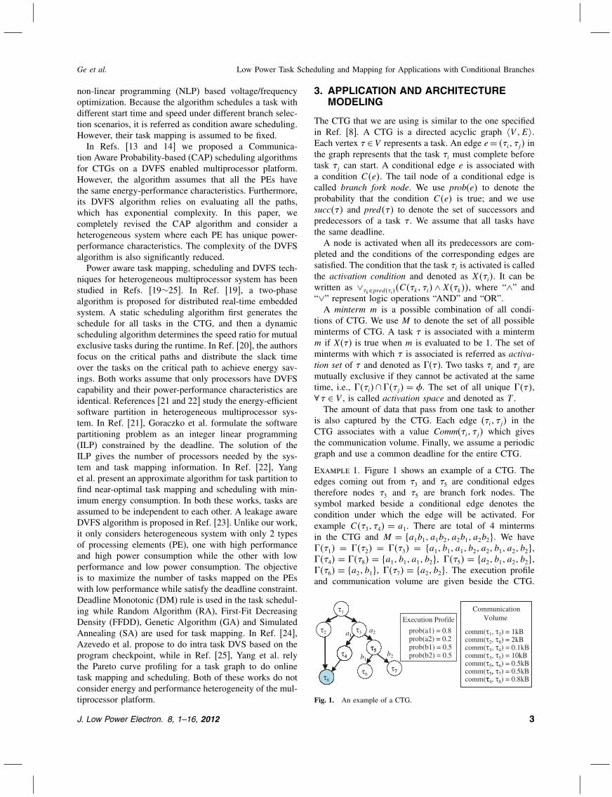
Example 1. Figure 1 shows an example of a CTG. Theedges coming out from �3 and �5 are conditional edgestherefore nodes �3 and �5 are branch fork nodes. Thesymbol marked beside a conditional edge denotes thecondition under which the edge will be activated. Forexample C��3� �4� = a1. There are total of 4 mintermsin the CTG and M = �a1b1� a1b2� a2b1� a2b2�. We have��1� = ��2� = ��3� = �a1� b1� a1� b2� a2� b1� a2� b2�,��4� = ��8� = �a1� b1� a1� b2�, ��5� = �a2� b1� a2� b2�,��6� = �a2� b1�, ��7� = �a2� b2�. The execution profileand communication volume are given beside the CTG.

τ1

τ8

τ3

τ6

τ5

τ2

τ7

a1a2

b1b2

prob(a1) = 0.8prob(a2) = 0.2prob(b1) = 0.5prob(b2) = 0.5

Execution Profile

comm(τ1, τ2) = 1kBcomm(τ2, τ8) = 2kBcomm(τ3, τ4) = 0.1kBcomm(τ3, τ5) = 10kBcomm(τ5, τ6) = 0.5kBcomm(τ5, τ7) = 0.5kBcomm(τ4, τ8) = 0.8kB

CommunicationVolume

τ4

τ1

τ8

τ55

7

1

, ,

τ

4

Fig. 1. An example of a CTG.

J. Low Power Electron. 8, 1–16, 2012 3


The activation space is:

T = {�a1b1� a1b2� a2b1� a2b2�� a1b1� a1b2��

�a2b1� a2b2�� a2b1�� a2b2�}

�

The hardware platform consists of a set of N PEs PE =�p1� p2� � pN . We use WCET ��i� pj�, �i ∈ V � pj ∈ PE,to denote the worst case execution time of task �i on pro-cessor pj . WCET ��i� pj� is expressed in the number ofclock cycles. We use BW�pipj� to denote the transmissionbandwidth of the communication links between pi and pj .A PE pi in the hardware platform is DVFS enabled.

Without loss of generality, we assume that its dynamiccycle energy Ei�dyn, which is the accumulated dynamicpower consumption during a clock cycle, is a convexand monotonically decreasing function of clock period T ,and − < dEi�dyn�T �/dT < 0� Tmin ≤ T ≤ Tmax. Its over-all cycle energy, Ei� total is calculated as Ei� total�T � =Ei� leak�T �+ Ei�dyn�T �. From Ref. [30], leakage currentIleak has an exponential relation (convex) against Vdd,while Vdd is inversely proportional (convex) to T , i.e.,Vdd ∝ f = 1/T . Therefore, Ileak has a convex relationagainst T . Furthermore, because Ei� leak = IleakVddT ∝ Ileak,Ei� total�T � is still a convex function of T

Theorem 1. There is an optimal clock period T ∗ that min-imizes the Ei� total�T � and Ei� total�T � is a convex and mono-tonically decreasing function for Tmin ≤ T ≤ T ∗.

Proof. Because Ei� total�T � is a convex function of T ,due to the property of convex function, there is a T ∗ ∈Tmin� Tmax� such that T ∗ minimizes Etotal�T � and Etotal�T �is a decreasing function for Tmin ≤ T ≤ T ∗. �

We refer T ∗ and f ∗clk = 1/T ∗ as break even clock period

and break even clock frequency. Our DVFS algorithmexplores the convex relation between Etotal and the clockperiod. We limit our DVFS algorithms to choose clockfrequencies in the range f ∗

clk� fmax�, where f ∗clk and fmax

are break even and maximum clock frequency of the sys-tem. In this range the total cycle energy will monotonicallydecrease as the clock period increases. Note that the proofof Theorem 1 assumes that the Edyn�T � and Etotal�T � arecontinuous functions. In Section 5, we will discuss how togeneralize the proposed DVFS algorithm to discrete volt-age and frequency scaling.

4. TASK MAPPING AND SCHEDULING

Our task mapping and scheduling is based on a modifiedDynamic Level based Scheduling (DLS)11 algorithm thatfinds task mapping and ordering simultaneously. Our goalis to implement an on-line scheduling, mapping DVFSalgorithm that adaptively change with the branch proba-bility. That’s why we choose the DL-based approach. TheDLS algorithm is a list scheduling algorithm. It maintainsa ready list that stores tasks whose predecessors have been

scheduled and mapped. For each task �i in the ready list,the dynamic level DL(�i, pj� is calculated using the fol-lowing equation:

DL��i� pj�= SL��i�−AT ��i� pj� (1)

where pj is one of the processing elements, SL(�i� is thestatic level of task �i, which is equal to the longest distancefrom node �i to any of the end nodes in the task graph (i.e.,the longest remaining execution time), AT ��i� pj� is theearliest time that task �i can start at processor pj , it is cal-culated as AT ��i� pj� = max DA��i� pj�� TF �pj��, whereDA(�i, pj� is the earliest time that all data required by node�i is available at the jth PE with the consideration of bothcomputation and communication delay, and TF(pj� is thetime that the last task assigned to the jth PE finishes itsexecution. The pair of (�i, pj� which gives the maximumdynamic level will be selected and the mapping is per-formed accordingly. The task is scheduled to be started atthe time max DA��i� pj�� TF �pj��. After that, the readylist is updated and the dynamic level of each task in theready list is re-calculated. The general flow of the DLSalgorithm is given in Algorithm 0. Because we need tocalculate the DL for each task processor pair in the sys-tem, the complexity of the DLS algorithm is O��V � ∗N�,where �V � is the number of tasks and N is the number ofPEs in the system.The original DLS algorithm does not handle mutual

exclusive tasks. Its goal is to minimize the makespan ofthe application. Although minimal makespan schedulingusually enables more aggressive DVFS and hence lowerpower consumption in a homogenous multi-core system,this is not always true in a heterogeneous system. In thiswork we adopt the general flow of the DLS algorithm butmodify the way that the dynamic level (DL) is calculatedto consider the mutual exclusiveness among conditionaltasks, the probability of branch selection and the energyperformance heterogeneity among processors.

Algorithm 0. General flow of DLS algorithmAlg. 0: DSL1. Calculate SL for each task2. ready_list=�;3. While (not all tasks have been scheduled) {4. For each pair (� , p), � is a ready task and

p ∈ PE, calculate DL��p�;5. Select the pair (�i, pj ) with the maximum DL;6. Map the task �i to processor pj and set its start

time to AT ��i� pj�;7. ready_list= ready_list∪ �i8. }

4.1. Minimum Average Makespan CTG Scheduling

Our first step is to modify the DL function to explore themutual exclusiveness among conditional tasks and con-sider the branch selection probability. The goal of such



modification is to minimize the average makespan insteadof the worst case makespan of the application. In the mod-ified algorithm, the static level (SL) of a task � is usedto represent the average remaining execution time when �has just started.The static level of a non-branching node is the maxi-

mum static level of its successors plus the average WCET(denoted as WCETavg� of itself. Let Succ(�i� be the setof successors of �i, Eq. (2) calculates the SL of a non-branching node.

SL��i�=WCET avg��i�+max�j SL��j�� j ∈Succ��i� (2)

The static level of a branch fork node is the mean of thestatic level of all its successors plus the WCETavg of itself.Let cij denote the condition of edge ��i� �j�, Eq. (3) calcu-lates the static level of a branch fork node.

SL��i�=WCET avg��i�+∑j

prob�cij �SL��j��

�j ∈ Succ��i� (3)

where prob�cij � is the probability that condition cij is true.For a task �i without successors, its static level equals

to its average worst case execution time: SL��i� =WCET avg��i�.The dynamic level of task-processor pair (�i, pj� is cal-

culated as the following equation.

DL��i� pj�= SL��i�−AT ��i� pj�+��i� pj� (4)

The term ��i� pj� is the difference between WCETavg(�i�and WCET ��i� pj� which accounts for the performanceheterogeneity. Adding this offset ensures correct evalua-tion of a task’s DL for different processors since SL iscomputed using the average WCET. AT ��i� pj� is the ear-liest time that task �i can start on processor pj . It mustsatisfy the following two conditions:1. At time AT ��i� pi� all data required by �i is availableat pi, i.e., AT ��i� pi�≥DA��i� pi�.2. If a task �j is scheduled during the interval AT ��i� pi��AT ��i� pi�+WCET ��i� pi��, then �j and �i are mutuallyexclusive. This condition allows two mutually exclusivetasks to share the same processor at the same time, andthus making the schedule more efficient.

The data available time of a task �i on processor pj iscalculated as the latest time when its predecessor com-pleted execution plus the time to transfer the data, i.e.,DA��i� pj� = max� ′ ET ��

′�+ comm�� ′� �i�/BW�p′� pj��,∀ � ′ ∈ pred��i�, where p′ is the processor where � ′ ismapped to and ET(� ′) is the end time of task � ′. Here weassume point to point communication between two pro-cessors. Please note that we can extend the framework tosystems with shared communication links by consideringall data communications as separate tasks and all commu-nication links as separate resources and schedule commu-nication tasks in the similar way as the computation tasks.

Please note that our DLS algorithm could also handle theoverhead of reconfiguring voltage and frequency by addingthe overhead to the variable AT ��i� pj�.

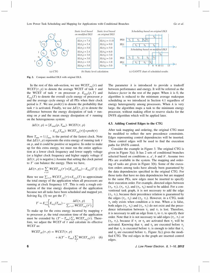
Example 2. Consider the CTG given in Figure 2(a). TheWCET of each task is marked beside the node. Thebranches a1 and a2 are taken with probability 0.9 and 0.1.The system has 2 PEs. In order to simplify the discus-sion, we assume that both PEs are identical and the inter-processor communication is negligible. Figure 2(b) givesthe static level of each task calculated using our modi-fied DLS and the original DLS. As we can see, SL��4� isgreater than SL��5� and SL��6� in the original DLS whiletheir relations are reversed in the modified DLS. This isbecause the original DLS considers the worst case perfor-mance, which happens along the path �4–�5, disregardingthe fact that task �5 is rarely activated. Figure 2(c) givesthe schedule found by these two DLS algorithms. In bothcases, �7 and �8 are scheduled to start on the same pro-cessor at the same time because these two tasks are mutu-ally exclusive. Using the original DLS, �4 is mapped andscheduled before �5 and �6 because the SL(�4) is greaterthan SL(�5) and SL(�6). This order is reversed in the mod-ified DLS. The worst case makespan of application sched-uled using the original and the modified DLS are 11 and13 respectively. However the average makespan is 11×01+10×09= 101 for the original DLS and 13×01+9×09= 94 for the modified DLS. �

4.2. Balancing Energy and Performance in aHeterogeneous Platform

In a homogenous system, because all PEs are identical inenergy performance characteristics, the total energy dissi-pation is determined solely by the slowdown ratio. Mini-mizing the average makespan will generally produce moreslacks for each task and enable a lower execution speedfor more energy reduction. Such monotonic relation doesnot exist in heterogeneous system, where the applicationenergy dissipation does not only depend on the slowdownratio, but also on which core the application is mapped to.There is a fundamental tradeoff between energy and per-

formance in a heterogeneous system. Mapping a task �to a faster PE could result better performance and shorterexecution time but will incur higher energy consumption.To compensate the extra energy incurred by task � , latertasks have to choose slower PEs to run and result longerlatency. The performance gain by running task � at fasterspeed will diminish. From this perspective, higher energyconsumption is equivalent to longer execution latency. Ourmodified DLS algorithm is already capable of handlingperformance heterogeneity among PEs (by introducing��i� pj� in Eq. (4)), to further consider energy hetero-geneity in the algorithm, we propose a heuristic methodto convert energy heterogeneity into performance hetero-geneity, and handle them in a unified way.



τ1

τ 2 τ3

τ4

τ8τ7

τ6 τ5

2

32

13 3

15

a1 a2

(a) CTG

SL(τ1) = 7.4SL(τ2) = 5.4SL(τ3) = 5.0

SL(τ4) = 2.4SL(τ5) = 3.0SL(τ6) = 3.0SL(τ7) = 1.0SL(τ8) = 5.0

SL(τ1) = 11.0SL(τ2) = 9.0SL(τ3) = 5.0

SL(τ4) = 6.0SL(τ5) = 3.0SL(τ6) = 3.0SL(τ7) = 1.0SL(τ8) = 5.0

Static level basedon modified DLS

Static level basedon original DLS

(b) Static level calculation

t

τ1 τ2 τ4 τ7

τ8

τ3 τ5 τ6

τ1 τ2

τ4

τ7

τ8

τ3 τ5

τ6

7 8 10 11 13 t

(c) GANTT chart of scheduled results

Scheduling based on original DLS

Scheduling based on modified DLS

PE0

0 9

PE1

PE0

PE1

Fig. 2. Compare modified DLS with original DLS.

In the rest of this sub-section, we use WCET avg�� andWCET��p� to denote the average WCET of task � andthe WCET of task � on processor p. Etotal�p�T � andEavg�T � to denote the overall cycle energy of processor pand the average cycle energy of all PEs when their clockperiod is T . We use prob(�) to denote the probability thattask � is activated. Finally, we use E��p� to denote thedifference between the energy dissipation of task � run-ning on p and the mean energy dissipation of � runningon the heterogeneous system:

E��p� = Etotal�p�Tmin� ·WCET��p�

−Eavg�Tmin� ·WCET avg��∗prob��Here Tmin = 1/fmax is the period of the fastest clock. Notethat E��p� represents the extra energy of running task �on p, and it could be positive or negative. In order to makeup for this extra energy, we must run the entire applica-tion at a lower clock frequency and lower supply voltage(or a higher clock frequency and higher supply voltage if E��p� is negative.) Assume that setting the clock periodto T ′ can balance the energy. Then we have,

E��p�= ∑� ′∈V

WCET avg��′�∗Eavg�Tmin�−Eavg�T

′�� (5)

Here we use∑

�∈V WCET avg��∗Eavg�T � to approximatethe total energy of the application when all processors arerunning at clock frequency 1/T . This is only a rough esti-mation of the true energy dissipation of the applicationbecause not all tasks have been scheduled and mapped yet.Solving Eq. (5) we get the T ′:

T ′ = E−1avg

[Eavg�Tmin�−

E��p�∑� ′∈V WCET avg��

′�

]

To make up for the extra energy incurred by mapping �to processor p, the total execution time of the applicationmust be extended by �T ′ − Tmin�

∑� WCET avg��. There-

fore, we adjust the WCET of � and calculate its effectiveWCET as:

WCET eff��p� = WCET ��p�

+��T ′ −Tmin�∑�

WCET avg�� (6)

The parameter � is introduced to provide a tradeoffbetween performance and energy. It will be referred as thebalance factor in the rest of the paper. When � is 0, thealgorithm is reduced to the minimum average makespanscheduling as we introduced in Section 4.1 regardless ofenergy heterogeneity among processors. When � is verylarge, the algorithm maps a task to the minimum energyprocessor, without making effort to reserve slacks for theDVFS algorithm which will be applied later.

4.3. Adding Control Edges to the CTG

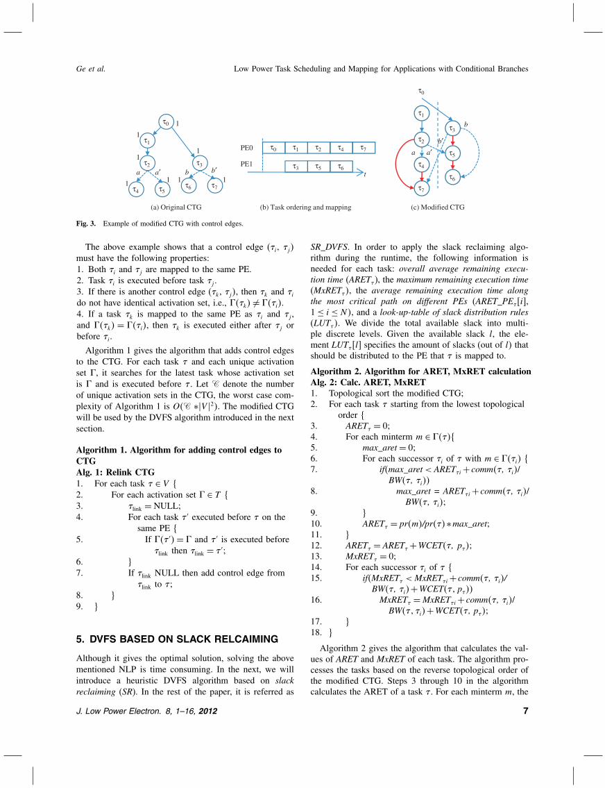
After task mapping and ordering, the original CTG mustbe modified to reflect the new precedence constraints.Edges representing control dependencies will be inserted.These control edges will be used to find the executionpaths for DVFS control.Consider the example in Figure 3. The original CTG is

given in Figure 3(a). It has 2 sets of conditional branchesselected based on conditions a, a′, b and b′. Assume twoPEs are available in the system. The mapping and order-ing of tasks are given in Figure 3(b). Some of the execu-tion orders among tasks have already been guaranteed bythe data dependencies specified in the original CTG. Forthose tasks that have no data dependencies but are mappedto the same PEs, new edges must be inserted to specifytheir execution order. For example, directed edges between(�4, �7�, (�3, �5�, and (�5, �6� need to be added. For a con-ventional task graph, it is not necessary to add the edge(�2, �7�, because their precedence relation is guaranteed bythe edges (�2, �4� and (�4, �7�. However, in a CTG, node�4 only exists when condition a is true. When a is false,both edges (�2, �4� and (�4, �7� do not exist and the prece-dence information between �2 and �7 is lost. Therefore,it is necessary to add an edge from �2 to �7 to specify theirorder. Note that it is not necessary to add edges (�1, �7� or(�0, �7�, because if �1 or �0 are activated then �2 will beactivated. Knowing that �1 and �0 are executed before �2and that �2 is executed before �7 is enough to infer that �1and �0 are executed before �7. Figure 3(c) gives the modi-fied CTG. The red edges in the graph are inserted controledges.



τ1

τ2

τ3

τ5

τ4

τ6

τ7

a a′

(c) Modified CTG

b

b′

τ0

τ0

τ2 τ3

τ5τ4τ6 τ7

1

11

1 11 1a a′

(a) Original CTG

b b′

τ11

t

τ1 τ2 τ4 τ7

τ3 τ5 τ6

(b) Task ordering and mapping

PE0

PE1

τ0

Fig. 3. Example of modified CTG with control edges.

The above example shows that a control edge (�i, �j�must have the following properties:1. Both �i and �j are mapped to the same PE.2. Task �i is executed before task �j .3. If there is another control edge (�k, �j�, then �k and �ido not have identical activation set, i.e., ��k� �= ��i�.4. If a task �k is mapped to the same PE as �i and �j ,and ��k� = ��i�, then �k is executed either after �j orbefore �i.

Algorithm 1 gives the algorithm that adds control edgesto the CTG. For each task � and each unique activationset � , it searches for the latest task whose activation setis � and is executed before � . Let � denote the numberof unique activation sets in the CTG, the worst case com-plexity of Algorithm 1 is O�� ∗�V �2�. The modified CTGwill be used by the DVFS algorithm introduced in the nextsection.

Algorithm 1. Algorithm for adding control edges toCTGAlg. 1: Relink CTG1. For each task � ∈ V {2. For each activation set � ∈ T {3. �link = NULL;4. For each task � ′ executed before � on the

same PE {5. If �� ′�= � and � ′ is executed before

�link then �link = � ′;6. }7. If �link NULL then add control edge from

�link to � ;8. }9. }

5. DVFS BASED ON SLACK RELCAIMING

Although it gives the optimal solution, solving the abovementioned NLP is time consuming. In the next, we willintroduce a heuristic DVFS algorithm based on slackreclaiming (SR). In the rest of the paper, it is referred as

SR_DVFS. In order to apply the slack reclaiming algo-rithm during the runtime, the following information isneeded for each task: overall average remaining execu-tion time (ARET� ), the maximum remaining execution time(MxRET� �, the average remaining execution time alongthe most critical path on different PEs (ARET_PE� [i],1≤ i ≤ N�, and a look-up-table of slack distribution rules(LUT� �. We divide the total available slack into multi-ple discrete levels. Given the available slack l, the ele-ment LUT� [l] specifies the amount of slacks (out of l� thatshould be distributed to the PE that � is mapped to.

Algorithm 2. Algorithm for ARET, MxRET calculationAlg. 2: Calc. ARET, MxRET1. Topological sort the modified CTG;2. For each task � starting from the lowest topological

order {3. ARET� = 0;4. For each minterm m ∈ ��{5. max_aret= 0;6. For each successor �i of � with m ∈ ��i� {7. if�max_aret< ARET�i+ comm�� , �i�/

BW�� , �i��8. max_aret = ARET�i+ comm�� , �i�/

BW�� , �i�;9. }10. ARET� = pr�m�/pr��∗max_aret;11. }12. ARET� = ARET� +WCET�� , p��;13. MxRET� = 0;14. For each successor �i of � {15. if�MxRET� <MxRET�i+ comm�� , �i�/

BW�� , �i�+WCET��p��16. MxRET� =MxRET�i+ comm�� , �i�/

BW�� i�+WCET�� , p� �;17. }18. }

Algorithm 2 gives the algorithm that calculates the val-ues of ARET and MxRET of each task. The algorithm pro-cesses the tasks based on the reverse topological order ofthe modified CTG. Steps 3 through 10 in the algorithmcalculates the ARET of a task � . For each minterm m, the



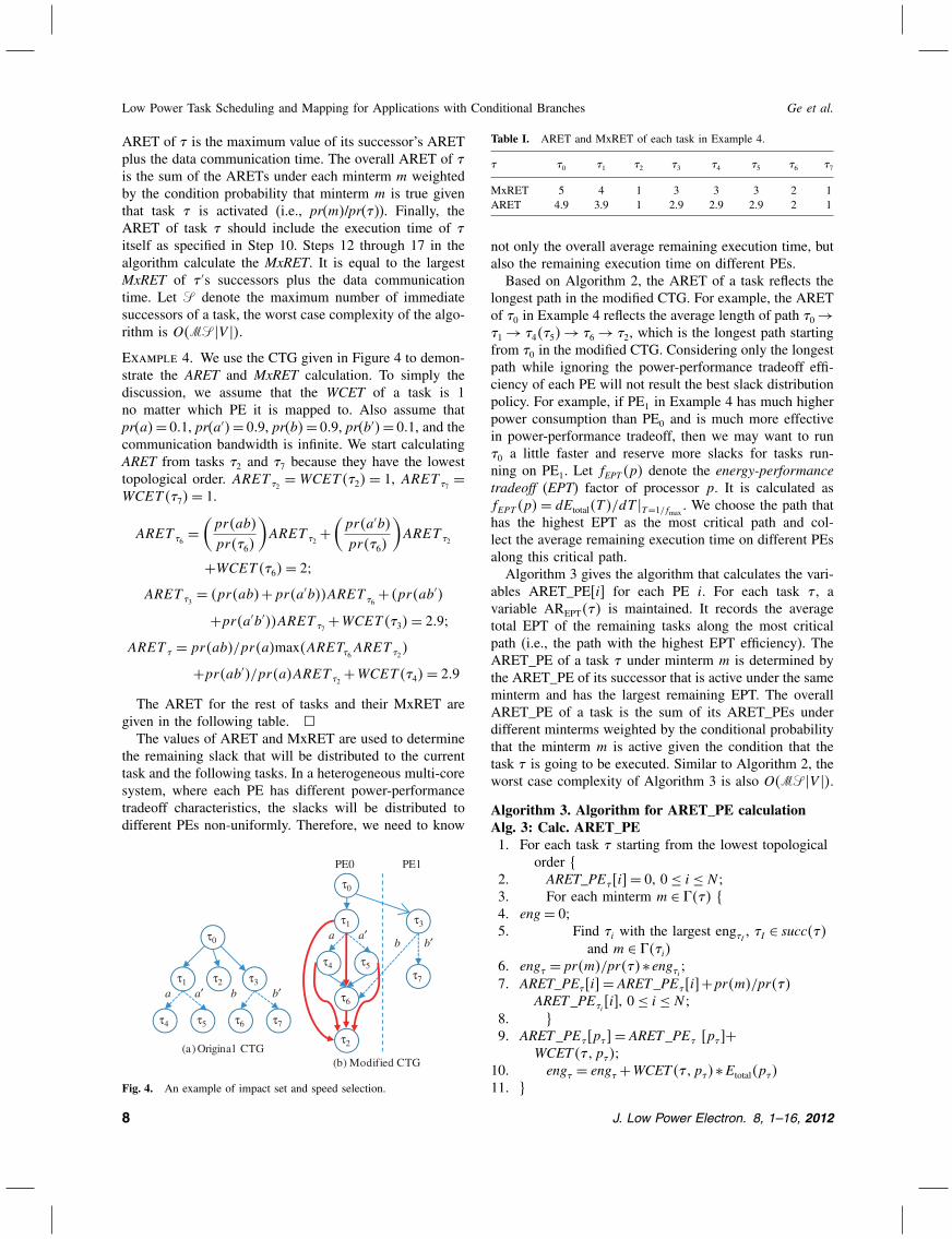
ARET of � is the maximum value of its successor’s ARETplus the data communication time. The overall ARET of �is the sum of the ARETs under each minterm m weightedby the condition probability that minterm m is true giventhat task � is activated (i.e., pr(m�/pr(�)). Finally, theARET of task � should include the execution time of �itself as specified in Step 10. Steps 12 through 17 in thealgorithm calculate the MxRET. It is equal to the largestMxRET of � ′s successors plus the data communicationtime. Let � denote the maximum number of immediatesuccessors of a task, the worst case complexity of the algo-rithm is O�� V ��.Example 4. We use the CTG given in Figure 4 to demon-strate the ARET and MxRET calculation. To simply thediscussion, we assume that the WCET of a task is 1no matter which PE it is mapped to. Also assume thatpr(a�= 01, pr(a′�= 09, pr(b�= 09, pr(b′�= 01, and thecommunication bandwidth is infinite. We start calculatingARET from tasks �2 and �7 because they have the lowesttopological order. ARET �2

=WCET ��2� = 1, ARET �7=

WCET ��7�= 1.

ARET �6=

(pr�ab�

pr��6�

)ARET �2

+(pr�a′b�pr��6�

)ARET �2

+WCET ��6�= 2�

ARET �3= �pr�ab�+pr�a′b��ARET �6

+ �pr�ab′�

+pr�a′b′��ARET �7+WCET ��3�= 29�

ARET � = pr�ab�/pr�a�max�ARET�6ARET �2�

+pr�ab′�/pr�a�ARET �2+WCET ��4�= 29

The ARET for the rest of tasks and their MxRET aregiven in the following table. �

The values of ARET and MxRET are used to determinethe remaining slack that will be distributed to the currenttask and the following tasks. In a heterogeneous multi-coresystem, where each PE has different power-performancetradeoff characteristics, the slacks will be distributed todifferent PEs non-uniformly. Therefore, we need to know

τ0

τ1 τ3

τ5τ4 τ6 τ7

a a′

(a) Original CTG

b b′τ2

(b) Modified CTG

τ0

τ1

τ5τ4

τ6

τ7

τ3

a a′b b′

τ2

PE0 PE1

Fig. 4. An example of impact set and speed selection.

Table I. ARET and MxRET of each task in Example 4.

� �0 �1 �2 �3 �4 �5 �6 �7

MxRET 5 4 1 3 3 3 2 1ARET 4.9 3.9 1 2.9 2.9 2.9 2 1

not only the overall average remaining execution time, butalso the remaining execution time on different PEs.Based on Algorithm 2, the ARET of a task reflects the

longest path in the modified CTG. For example, the ARETof �0 in Example 4 reflects the average length of path �0 →�1 → �4��5�→ �6 → �2, which is the longest path startingfrom �0 in the modified CTG. Considering only the longestpath while ignoring the power-performance tradeoff effi-ciency of each PE will not result the best slack distributionpolicy. For example, if PE1 in Example 4 has much higherpower consumption than PE0 and is much more effectivein power-performance tradeoff, then we may want to run�0 a little faster and reserve more slacks for tasks run-ning on PE1. Let fEPT �p� denote the energy-performancetradeoff (EPT) factor of processor p. It is calculated asfEPT �p�= dEtotal�T �/dT �T=1/fmax

. We choose the path thathas the highest EPT as the most critical path and col-lect the average remaining execution time on different PEsalong this critical path.Algorithm 3 gives the algorithm that calculates the vari-

ables ARET_PE[i] for each PE i. For each task � , avariable AREPT�� is maintained. It records the averagetotal EPT of the remaining tasks along the most criticalpath (i.e., the path with the highest EPT efficiency). TheARET_PE of a task � under minterm m is determined bythe ARET_PE of its successor that is active under the sameminterm and has the largest remaining EPT. The overallARET_PE of a task is the sum of its ARET_PEs underdifferent minterms weighted by the conditional probabilitythat the minterm m is active given the condition that thetask � is going to be executed. Similar to Algorithm 2, theworst case complexity of Algorithm 3 is also O�� V ��.Algorithm 3. Algorithm for ARET_PE calculationAlg. 3: Calc. ARET_PE1. For each task � starting from the lowest topological

order {2. ARET_PE� i�= 0, 0 ≤ i ≤ N ;3. For each minterm m ∈ �� {4. eng= 0;5. Find �i with the largest eng�I , �I ∈ succ��

and m ∈ ��i�6. eng� = pr�m�/pr��∗ eng�i ;7. ARET_PE� i�= ARET_PE� i�+pr�m�/pr��

ARET_PE�ii�, 0 ≤ i ≤ N ;

8. }9. ARET_PE� p��= ARET_PE� p��+

WCET��p��;10. eng� = eng� +WCET��p��∗Etotal�p��11. }



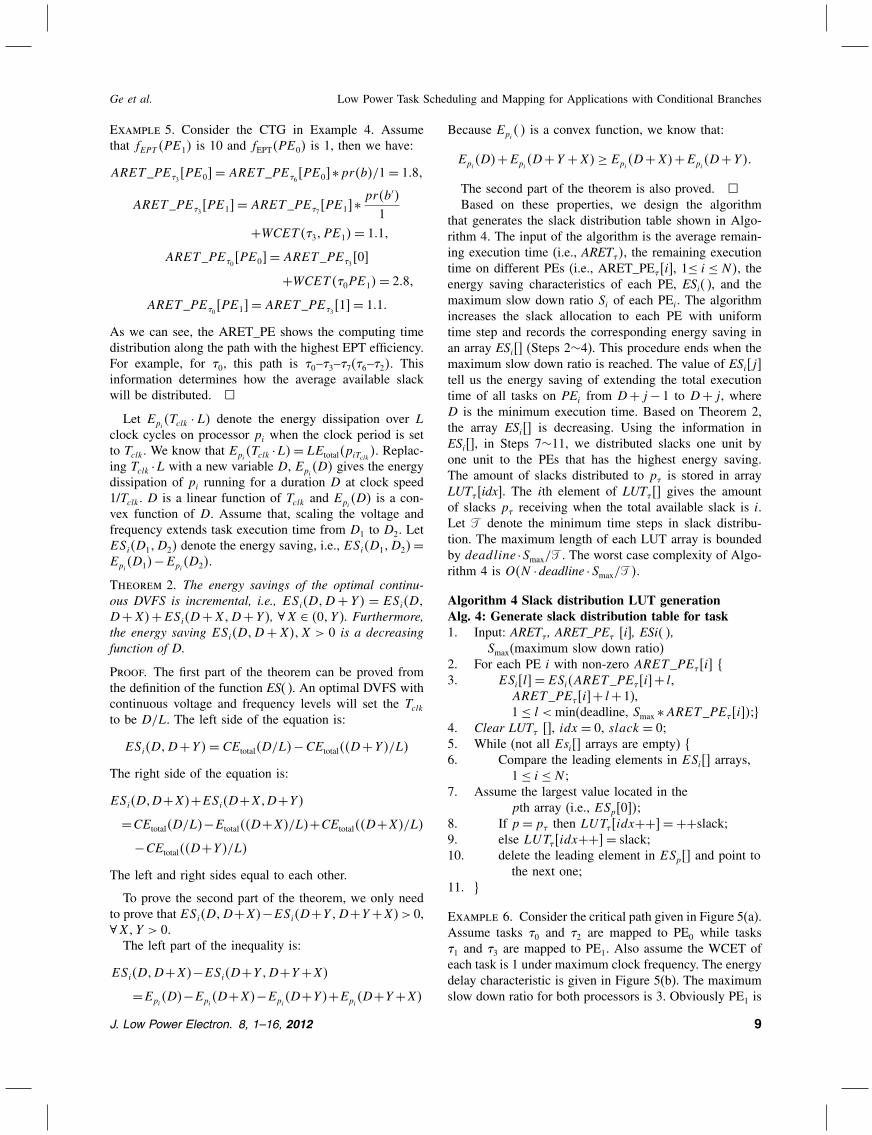
Example 5. Consider the CTG in Example 4. Assumethat fEPT �PE1� is 10 and fEPT�PE0� is 1, then we have:

ARET _PE�3PE0�= ARET _PE�6

PE0�∗pr�b�/1= 18�


PE1�∗pr�b′�

1

+WCET ��3� PE1�= 11�


0�

+WCET ��0PE1�= 28�


1�= 11

As we can see, the ARET_PE shows the computing timedistribution along the path with the highest EPT efficiency.For example, for �0, this path is �0–�3–�7(�6–�2�. Thisinformation determines how the average available slackwill be distributed. �

Let Epi�Tclk ·L� denote the energy dissipation over L

clock cycles on processor pi when the clock period is setto Tclk. We know that Epi

�Tclk ·L�= LEtotal�piTclk�. Replac-

ing Tclk ·L with a new variable D, Epi�D� gives the energy

dissipation of pi running for a duration D at clock speed1/Tclk. D is a linear function of Tclk and Epi

�D� is a con-vex function of D. Assume that, scaling the voltage andfrequency extends task execution time from D1 to D2. LetESi�D1�D2� denote the energy saving, i.e., ESi�D1�D2�=Epi

�D1�−Epi�D2�.

Theorem 2. The energy savings of the optimal continu-ous DVFS is incremental, i.e., ESi�D�D+ Y � = ESi�D�D+X�+ESi�D+X�D+Y �, ∀X ∈ �0� Y �. Furthermore,the energy saving ESi�D�D+X��X > 0 is a decreasingfunction of D.

Proof. The first part of the theorem can be proved fromthe definition of the function ES( ). An optimal DVFS withcontinuous voltage and frequency levels will set the Tclkto be D/L. The left side of the equation is:

ESi�D�D+Y �= CEtotal�D/L�−CEtotal��D+Y �/L�

The right side of the equation is:

ESi�D�D+X�+ESi�D+X�D+Y �

=CEtotal�D/L�−Etotal��D+X�/L�+CEtotal��D+X�/L�

−CEtotal��D+Y �/L�

The left and right sides equal to each other.

To prove the second part of the theorem, we only needto prove that ESi�D�D+X�−ESi�D+Y �D+Y +X�> 0,∀X�Y > 0.

The left part of the inequality is:

ESi�D�D+X�−ESi�D+Y �D+Y +X�

=Epi�D�−Epi

�D+X�−Epi�D+Y �+Epi

�D+Y +X�

Because Epi� � is a convex function, we know that:

Epi�D�+Epi

�D+Y +X�≥ Epi�D+X�+Epi

�D+Y �

The second part of the theorem is also proved. �

Based on these properties, we design the algorithmthat generates the slack distribution table shown in Algo-rithm 4. The input of the algorithm is the average remain-ing execution time (i.e., ARET� �, the remaining executiontime on different PEs (i.e., ARET_PE� [i], 1≤ i ≤ N�, theenergy saving characteristics of each PE, ESi( ), and themaximum slow down ratio Si of each PEi. The algorithmincreases the slack allocation to each PE with uniformtime step and records the corresponding energy saving inan array ESi[] (Steps 2∼4). This procedure ends when themaximum slow down ratio is reached. The value of ESi[j]tell us the energy saving of extending the total executiontime of all tasks on PEi from D+ j − 1 to D+ j , whereD is the minimum execution time. Based on Theorem 2,the array ESi[] is decreasing. Using the information inESi[], in Steps 7∼11, we distributed slacks one unit byone unit to the PEs that has the highest energy saving.The amount of slacks distributed to p� is stored in arrayLUT� [idx]. The ith element of LUT� [] gives the amountof slacks p� receiving when the total available slack is i.Let � denote the minimum time steps in slack distribu-tion. The maximum length of each LUT array is boundedby deadline ·Smax/� . The worst case complexity of Algo-rithm 4 is O�N ·deadline ·Smax/� �.

Algorithm 4 Slack distribution LUT generationAlg. 4: Generate slack distribution table for task1. Input: ARET� , ARET_PE� i�, ESi� �,

Smax(maximum slow down ratio)2. For each PE i with non-zero ARET _PE�i� {3. ESil�= ESi�ARET _PE�i�+ l,

ARET _PE�i�+ l+1),1≤ l <min(deadline, Smax ∗ARET _PE�i��;}

4. Clear LUT� [], idx = 0, slack = 0;5. While (not all Esi[] arrays are empty) {6. Compare the leading elements in ESi� arrays,

1≤ i ≤ N ;7. Assume the largest value located in the

pth array (i.e., ESp0��;8. If p = p� then LUT�idx++�=++slack;9. else LUT�idx++�= slack;10. delete the leading element in ESp� and point to

the next one;11. }

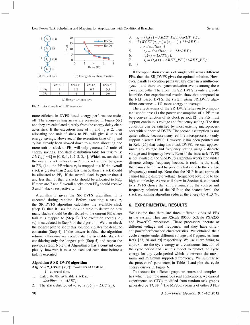
Example 6. Consider the critical path given in Figure 5(a).Assume tasks �0 and �2 are mapped to PE0 while tasks�1 and �3 are mapped to PE1. Also assume the WCET ofeach task is 1 under maximum clock frequency. The energydelay characteristic is given in Figure 5(b). The maximumslow down ratio for both processors is 3. Obviously PE1 is



(a) Critical Path

τ0

τ1

τ3

τ4

PE0

PE1

PE0

PE1

1

1

1

1

(b) Energy delay characteristics

0

5

10

15

20

0 2 4 6 8E

nerg

yDelay (D)

E0(D)

E1(D)

ES(2,3) ES(3,4) ES(4,5) ES(5,6)ES0 4 1.8 0.7 0.5ES1 8 4 1.5 0.9

(c) Energy saving arrays

Fig. 5. An example of LUT generation.

more efficient in DVFS based energy performance trade-off. The energy saving arrays are presented in Figure 5(c)and they are calculated directly from the energy delay char-acteristics. If the execution time of �0 and �2 is 2, thenallocating one unit of slack to PE1 will give 8 units ofenergy savings. However, if the execution time of �0 and�2 has already been slowed down to 4, then allocating onemore unit of slack to PE1 will only generate 1.5 units ofenergy savings. The slack distribution table for task �0 is:LUT �0

1∼8� = �0�0�1�1�2�2�3�4�. Which means that ifthe overall slack is less than 3, no slack should be givento PE0 (i.e., the PE where �0 is mapped to); if the overallslack is greater than 2 and less than 5, then 1 slack shouldbe allocated to PE0; if the overall slack is greater than 4and less than 7, then 2 slacks should be allocated to PE0.If there are 7 and 8 overall slacks, then PE0 should receive3 and 4 slacks respectively. �

Algorithm 5 gives the SR_DVFS algorithm. It isexecuted during runtime. Before executing a task � ,the SR_DVFS algorithm calculates the available slack(Step 1), then it uses the look-up-table to determine howmany slacks should be distributed to the current PE wheretask � is mapped to (Step 2). The execution speed (i.e.,s�� is calculated in Step 3 of the algorithm. We then checkthe longest path to see if this solution violates the deadlineconstraint (Step 4). If the answer is false, the algorithmreturns, otherwise we recalculate the available slack byconsidering only the longest path (Step 5) and repeat theprevious steps. Note that Algorithm 5 has a constant com-plexity; however, it must be executed each time before atask is executed.

Algorithm 5 SR_DVFS algorithmAlg. 5: SR_DVFS �� t�: �—current task id,

t—current time1. Calculate the available slack tsl =

deadline− t−ARET� ;2. The slack distributed to p� is tsl��= LUT �tsl�;

3. s� = �tsl��+ARET _PE��/ARET _PE� ;4. if (WCET �� , p��∗ �s� −1�+MxRET�+

t > deadline� {5. tsl = deadline− t−MxRET� ;6. tsl��= LUT �tsl�;7. s� = �tsl��+ARET _PE��/ARET _PE� ;8. }

If the application consists of single path across differentPEs, then the SR_DVFS gives the optimal solution. How-ever, parallel execution paths usually exist in a multi-coresystem and there are synchronization events among theseexecution paths. Therefore, the SR_DVFS is only a greedyheuristic. Our experimental results show that compared tothe NLP based DVFS, the system using SR_DVFS algo-rithm consumes 4.1% more energy in average.The effectiveness of the SR_DVFS relies on two impor-

tant conditions: (1) the power consumption of a PE mustbe a convex function of its clock period; (2) the PEs mustsupport continuous voltage and frequency scaling. The firstcondition can be satisfied by most existing microproces-sors with support of DVFS. The second assumption is notquite realistic, because many real life microprocessors onlysupport discrete DVFS. However, it has been pointed outin Ref. [26] that using intra-task DVFS, we can approx-imate any voltage and frequency setting using 2 discretevoltage and frequency levels. Even if the intra-task DVFSis not available, the SR-DVFS algorithm works fine underdiscrete voltage–frequency because it reclaims the slackthat cannot be utilized by previous tasks due to the voltage(frequency) round up. Note that the NLP based approachcannot handle discrete voltage (frequency) level due to thehigh complexity. As we will show in Section 6, comparedto a DVFS choice that simply rounds up the voltage andfrequency solution of the NLP to the nearest level, theslack reclaiming algorithm reduces the energy by 41.37%.

6. EXPERIMENTAL RESULTS

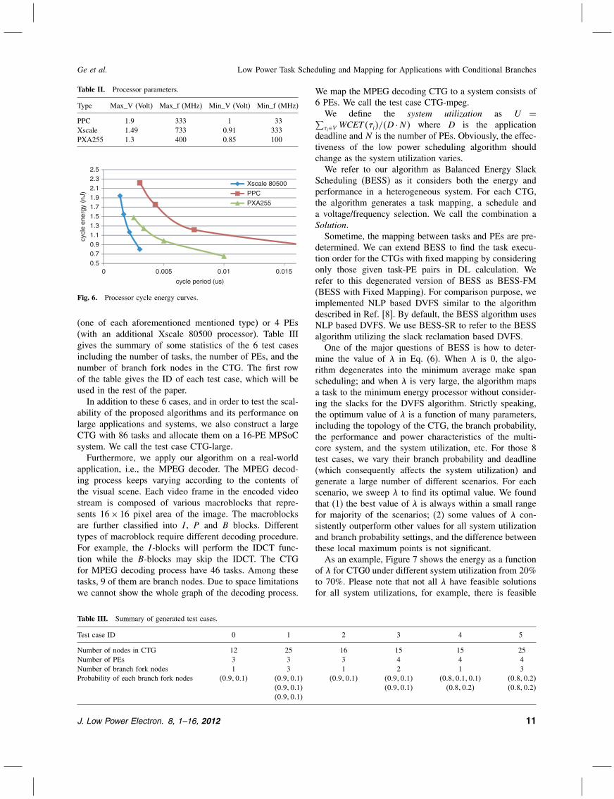
We assume that there are three different kinds of PEsin the system. They are XScale 80500, XScale PXA255and PowerPC processors. These processors operate atdifferent voltage and frequency, and they have differ-ent power/performance characteristics. We obtained theircycle energies under different voltage and frequencies fromRefs. [27, 28 and 29] respectively. We use curve fitting toapproximate the cycle energy as a continuous function ofthe cycle period and use this model to predict the cycleenergy for any cycle period which is between the maxi-mum and minimum supported frequency. We summarizethe processors’ parameters in Table II and plot the cycleenergy curves in Figure 6.To account for different graph structures and complexi-

ties which resemble numerous real applications, we carriedexperiments on CTGs modified from random task graphsgenerated by TGFF.12 The MPSoC consists of either 3 PEs



Table II. Processor parameters.

Type Max_V (Volt) Max_f (MHz) Min_V (Volt) Min_f (MHz)

PPC 19 333 1 33Xscale 149 733 0.91 333PXA255 13 400 0.85 100

0.50.70.91.11.31.51.71.92.12.32.5

0 0.005 0.01 0.015

cycl

e en

ergy

(nJ

)

cycle period (us)

Xscale 80500

PPC

PXA255

Fig. 6. Processor cycle energy curves.

(one of each aforementioned mentioned type) or 4 PEs(with an additional Xscale 80500 processor). Table IIIgives the summary of some statistics of the 6 test casesincluding the number of tasks, the number of PEs, and thenumber of branch fork nodes in the CTG. The first rowof the table gives the ID of each test case, which will beused in the rest of the paper.In addition to these 6 cases, and in order to test the scal-

ability of the proposed algorithms and its performance onlarge applications and systems, we also construct a largeCTG with 86 tasks and allocate them on a 16-PE MPSoCsystem. We call the test case CTG-large.Furthermore, we apply our algorithm on a real-world

application, i.e., the MPEG decoder. The MPEG decod-ing process keeps varying according to the contents ofthe visual scene. Each video frame in the encoded videostream is composed of various macroblocks that repre-sents 16× 16 pixel area of the image. The macroblocksare further classified into I , P and B blocks. Differenttypes of macroblock require different decoding procedure.For example, the I-blocks will perform the IDCT func-tion while the B-blocks may skip the IDCT. The CTGfor MPEG decoding process have 46 tasks. Among thesetasks, 9 of them are branch nodes. Due to space limitationswe cannot show the whole graph of the decoding process.

Table III. Summary of generated test cases.

Test case ID 0 1 2 3 4 5

Number of nodes in CTG 12 25 16 15 15 25Number of PEs 3 3 3 4 4 4Number of branch fork nodes 1 3 1 2 1 3Probability of each branch fork nodes �09�01� �09�01� �09�01� �09�01� �08�01�01� �08�02�

�09�01� �09�01� �08�02� �08�02��09�01�

We map the MPEG decoding CTG to a system consists of6 PEs. We call the test case CTG-mpeg.We define the system utilization as U =∑�i∈V WCET��i�/�D ·N� where D is the application

deadline and N is the number of PEs. Obviously, the effec-tiveness of the low power scheduling algorithm shouldchange as the system utilization varies.We refer to our algorithm as Balanced Energy Slack

Scheduling (BESS) as it considers both the energy andperformance in a heterogeneous system. For each CTG,the algorithm generates a task mapping, a schedule anda voltage/frequency selection. We call the combination aSolution.Sometime, the mapping between tasks and PEs are pre-

determined. We can extend BESS to find the task execu-tion order for the CTGs with fixed mapping by consideringonly those given task-PE pairs in DL calculation. Werefer to this degenerated version of BESS as BESS-FM(BESS with Fixed Mapping). For comparison purpose, weimplemented NLP based DVFS similar to the algorithmdescribed in Ref. [8]. By default, the BESS algorithm usesNLP based DVFS. We use BESS-SR to refer to the BESSalgorithm utilizing the slack reclamation based DVFS.One of the major questions of BESS is how to deter-

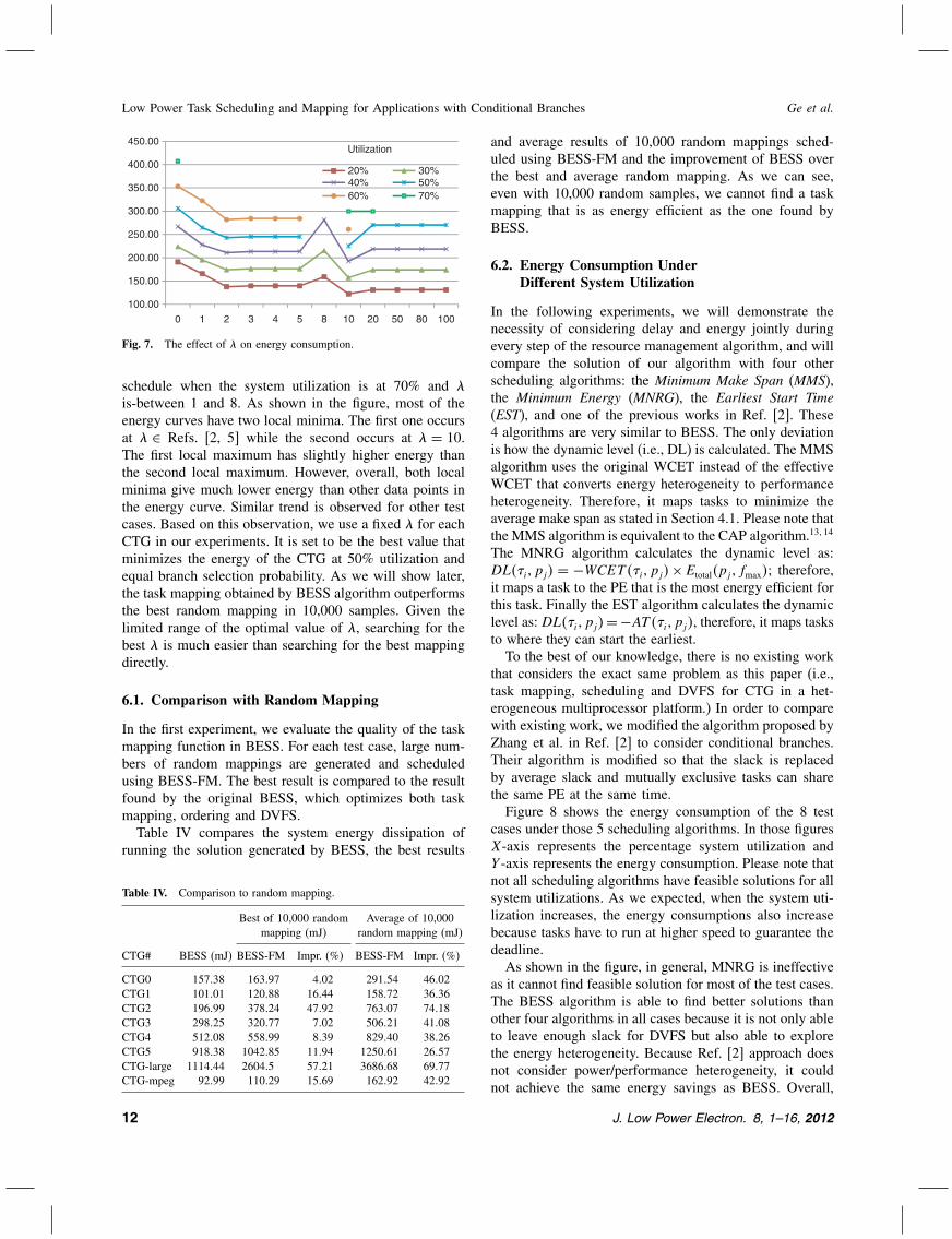
mine the value of � in Eq. (6). When � is 0, the algo-rithm degenerates into the minimum average make spanscheduling; and when � is very large, the algorithm mapsa task to the minimum energy processor without consider-ing the slacks for the DVFS algorithm. Strictly speaking,the optimum value of � is a function of many parameters,including the topology of the CTG, the branch probability,the performance and power characteristics of the multi-core system, and the system utilization, etc. For those 8test cases, we vary their branch probability and deadline(which consequently affects the system utilization) andgenerate a large number of different scenarios. For eachscenario, we sweep � to find its optimal value. We foundthat (1) the best value of � is always within a small rangefor majority of the scenarios; (2) some values of � con-sistently outperform other values for all system utilizationand branch probability settings, and the difference betweenthese local maximum points is not significant.As an example, Figure 7 shows the energy as a function

of � for CTG0 under different system utilization from 20%to 70%. Please note that not all � have feasible solutionsfor all system utilizations, for example, there is feasible



100.00

150.00

200.00

250.00

300.00

350.00

400.00

450.00

0 1 2 3 4 5 8 10 20 50 80 100

20% 30%40% 50%60% 70%

Utilization

Fig. 7. The effect of � on energy consumption.

schedule when the system utilization is at 70% and �is-between 1 and 8. As shown in the figure, most of theenergy curves have two local minima. The first one occursat � ∈ Refs. [2, 5] while the second occurs at � = 10.The first local maximum has slightly higher energy thanthe second local maximum. However, overall, both localminima give much lower energy than other data points inthe energy curve. Similar trend is observed for other testcases. Based on this observation, we use a fixed � for eachCTG in our experiments. It is set to be the best value thatminimizes the energy of the CTG at 50% utilization andequal branch selection probability. As we will show later,the task mapping obtained by BESS algorithm outperformsthe best random mapping in 10,000 samples. Given thelimited range of the optimal value of �, searching for thebest � is much easier than searching for the best mappingdirectly.

6.1. Comparison with Random Mapping

In the first experiment, we evaluate the quality of the taskmapping function in BESS. For each test case, large num-bers of random mappings are generated and scheduledusing BESS-FM. The best result is compared to the resultfound by the original BESS, which optimizes both taskmapping, ordering and DVFS.Table IV compares the system energy dissipation of

running the solution generated by BESS, the best results

Table IV. Comparison to random mapping.

Best of 10,000 random Average of 10,000mapping (mJ) random mapping (mJ)

CTG# BESS (mJ) BESS-FM Impr. (%) BESS-FM Impr. (%)

CTG0 15738 16397 402 29154 4602CTG1 10101 12088 1644 15872 3636CTG2 19699 37824 4792 76307 7418CTG3 29825 32077 702 50621 4108CTG4 51208 55899 839 82940 3826CTG5 91838 104285 1194 125061 2657CTG-large 111444 26045 5721 368668 6977CTG-mpeg 9299 11029 1569 16292 4292

and average results of 10,000 random mappings sched-uled using BESS-FM and the improvement of BESS overthe best and average random mapping. As we can see,even with 10,000 random samples, we cannot find a taskmapping that is as energy efficient as the one found byBESS.

6.2. Energy Consumption UnderDifferent System Utilization

In the following experiments, we will demonstrate thenecessity of considering delay and energy jointly duringevery step of the resource management algorithm, and willcompare the solution of our algorithm with four otherscheduling algorithms: the Minimum Make Span (MMS),the Minimum Energy (MNRG), the Earliest Start Time(EST), and one of the previous works in Ref. [2]. These4 algorithms are very similar to BESS. The only deviationis how the dynamic level (i.e., DL) is calculated. The MMSalgorithm uses the original WCET instead of the effectiveWCET that converts energy heterogeneity to performanceheterogeneity. Therefore, it maps tasks to minimize theaverage make span as stated in Section 4.1. Please note thatthe MMS algorithm is equivalent to the CAP algorithm.13�14

The MNRG algorithm calculates the dynamic level as:DL��i� pj� = −WCET ��i� pj�×Etotal�pj� fmax�; therefore,it maps a task to the PE that is the most energy efficient forthis task. Finally the EST algorithm calculates the dynamiclevel as: DL��i� pj�=−AT ��i� pj�, therefore, it maps tasksto where they can start the earliest.To the best of our knowledge, there is no existing work

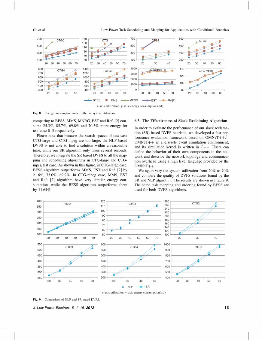
that considers the exact same problem as this paper (i.e.,task mapping, scheduling and DVFS for CTG in a het-erogeneous multiprocessor platform.) In order to comparewith existing work, we modified the algorithm proposed byZhang et al. in Ref. [2] to consider conditional branches.Their algorithm is modified so that the slack is replacedby average slack and mutually exclusive tasks can sharethe same PE at the same time.Figure 8 shows the energy consumption of the 8 test

cases under those 5 scheduling algorithms. In those figuresX-axis represents the percentage system utilization andY -axis represents the energy consumption. Please note thatnot all scheduling algorithms have feasible solutions for allsystem utilizations. As we expected, when the system uti-lization increases, the energy consumptions also increasebecause tasks have to run at higher speed to guarantee thedeadline.As shown in the figure, in general, MNRG is ineffective

as it cannot find feasible solution for most of the test cases.The BESS algorithm is able to find better solutions thanother four algorithms in all cases because it is not only ableto leave enough slack for DVFS but also able to explorethe energy heterogeneity. Because Ref. [2] approach doesnot consider power/performance heterogeneity, it couldnot achieve the same energy savings as BESS. Overall,



100

300

500

700

20 30 40 50 60 70

CTG0

50

70

90

110

130

150

20 30 40 50 60 70

CTG1

100

300

500

700

20 30 40

CTG2

200

400

600

800

20 30 40 50 60

CTG3

300

400

500

600

700

800

20 30 40 50

CTG4

400

600

800

1000

1200

1400

20 30 40 50 60

CTG5

0

1000

2000

3000

4000

20 30 40 50 60

CTG-large

80

100

120

140

20 30 40 50 60

CTG-mpeg

x-axis: utilization, y-axis: energy consumption (mJ)

BESS MMS MENG EST Ref[2]

Fig. 8. Energy consumption under different system utilization.

comparing to BESS, MMS, MNRG, EST and Ref. [2] con-sume 25.3%, 85.7%, 69.8% and 70.3% more energy fortest case 0–5 respectively.Please note that because the search spaces of test case

CTG-large and CTG-mpeg are too large, the NLP basedDVFS is not able to find a solution within a reasonabletime, while our SR algorithm only takes several seconds.Therefore, we integrate the SR based DVFS to all the map-ping and scheduling algorithms in CTG-large and CTG-mpeg test case. As shown in this figure, in CTG-large case,BESS algorithm outperforms MMS, EST and Ref. [2] by21.6%, 73.0%, 69.9%. In CTG-mpeg case, MMS, ESTand Ref. [2] algorithm have very similar energy con-sumption, while the BESS algorithm outperforms themby 11.64%.

100

150

200

250

300

350

400

20 30 40 50 60 70 20 30 40 50 60 70

CTG0

50

60

70

80

90

100

110

120CTG1

100120140160180200220240260280

20 30 40

CTG2

250

300

350

400

450

500

550

20 30 40 50 60

CTG3

300

350

400

450

500

550

600

20 30 40 50

CTG4

400

500

600

700

800

900

1000

20 30 40 50 60

CTG5

x-axis utilization, y-axis energy consumption(mJ)

NLP SR

Fig. 9. Comparison of NLP and SR based DVFS.

6.3. The Effectiveness of Slack Reclaiming Algorithm

In order to evaluate the performance of our slack reclama-tion (SR) based DVFS heuristic, we developed a fast per-formance evaluation framework based on OMNeT++.31

OMNeT++ is a discrete event simulation environment,and its simulation kernel is written in C++. Users candefine the behavior of their own components in the net-work and describe the network topology and communica-tion overhead using a high level language provided by theOMNeT++.We again vary the system utilization from 20% to 70%

and compare the quality of DVFS solutions found by theSR and NLP algorithm. The results are shown in Figure 9.The same task mapping and ordering found by BESS areused for both DVFS algorithms.



Table V. Comparison of continuous and discrete DVFS.

Continuous DVFS (mJ) Discrete DVFS (mJ)

CTGs NLP SR NLP SR

CTG 0 19264 20266 41529 21892CTG 1 7319 8034 18386 9282CTG 2 25359 26827 32129 27044CTG 3 37738 39475 6142 41848CTG 4 46483 49213 85952 49186CTG 5 69723 72179 19853 77560

As shown in these figures, the SR algorithm tracks theNPL based DVFS algorithm very well and gives closeenergy consumptions. In average, systems using SR basedDVFS method only consume 4.1% more energy than thesystem using NLP based DVFS.Table V shows the comparison between the continuous

and discrete DVFS. As shown in the table, the perfor-mance of NLP based DVFS is severely degraded whenonly discrete voltage and frequency level is supported bythe system, while the SR algorithm dynamically adjuststhe slowdown ratio based on current remaining slack. Onaverage, the discretized slack reclaiming algorithm reducesthe energy dissipation by 41.37% comparing to discretizedNLP algorithm. Please note that for test case CTG-largeCTG-mpeg, the only feasible DVFS algorithm is SlackReclaiming based algorithm, thus in this subsection, wedo not have results for them.In the next experiment we restrict the PE’s voltage and

frequency to those discrete levels specified in Table II.With NLP based DVFS, in order to guarantee deadline, thevoltage and frequency are always round up to the nearestlevel. With SR based DVFS, the extra slack generated byrounding up of current task will be reclaimed by futuretasks.

6.4. Sensitivity to Branch Probability Change

In previous experiments, we assume that the branch prob-abilities are known and fixed during run time. In the nextset of experiments, we examine the sensitivity of BESS tothe change of branch probability. The results will help usto understand the performance of BESS under inaccuratesoftware model or insufficient profiling information.The solution of BESS consists of 3 parts: task mapping,

task ordering and voltage/frequency selection. When thebranch probability of an application changes from � to� during the runtime, we have 4 options: (1) Continueusing the initial scheduling found based on branch prob-ability �. This option will be referred as “No update” asit updates nothing. (2) Continue using the original taskmapping and ordering, but update the voltage and fre-quency selection using the new branch probability �. Thisoption will be referred as “DVFS only.” (3) Continueusing the original task mapping, but update the task order-ing and voltage/frequency selection. It will be referred as

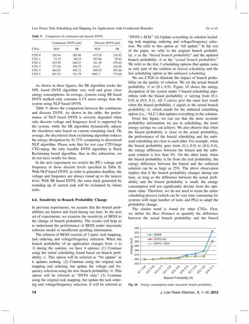
“DVFS+SCH.” (4) Update everything in solution includ-ing task mapping, ordering and voltage/frequency selec-tion. We refer to this option as “All update.” In the restof the paper, we refer to the original branch probabil-ity � as the “biased branch probability” and the updatedbranch probability � as the “actual branch probability.”We refer to the first 3 scheduling options that update noneor only part of the solution as biased scheduling and thelast scheduling option as the unbiased scheduling.We use CTG0 to illustrate the impact of branch proba-

bility on the quality of solution. We set the actual branchprobability � to �01�09�. Figure 10 shows the energydissipation of the system under 3 biased scheduling algo-rithms with the biased probability � varying from (0.1,0.9) to (0.9, 0.1). All 3 curves give the same best resultwhen the biased probability � equals to the actual branchprobability �, which stands for the unbiased schedulingoption (i.e., “ALL”) that updates everything in the solution.From this figure, we can see that the more accurate

probability information we use in scheduling, the moreenergy savings we can achieve. We also observe that whenthe biased probability is close to the actual probability,the performance of the biased scheduling and the unbi-ased scheduling are close to each other. For example, whenthe biased probability goes from �01�09� to �06�04�,the energy difference between the biased and the unbi-ased solution is less than 4%. On the other hand, whenthe biased probability is far from the real probability, theenergy difference between the biased and the unbiasedsolution can be as large as 25%. The above observationimplies that if the branch probability changes during runtime, as long as the difference between the actual prob-ability and the biased probability is small, the energyconsumption will not significantly deviate from the opti-mum value. Therefore, we do not need to rerun the entirescheduling process (which can be very time consuming forsystems with large number of tasks and PEs) to adapt theprobability change.The similar trend is found for other CTGs. First,

we define the Bias Distance to quantify the differencebetween the actual branch probability and the biased

250

260

270

280

290

300

310

320

330

(0.1

, 0.9

)

(0.2

, 0.8

)

(0.3

, 0.7

)

(0.4

, 0.6

)

(0.5

, 0.5

)

(0.6

, 0.4

)

(0.7

, 0.3

)

(0.8

, 0.2

)

(0.9

, 0.1

)

ener

gy (

mJ)

Biased Probability (A)

NONE

DVFS only

DVFS + SCH

Fig. 10. Energy consumption under inaccurate branch probability.



Table VI. Solution quality degradation as the bias distance increases.

0.2 0.4 0.6 0.8 1 1.2 1.4 1.6Bias distance (%) (%) (%) (%) (%) (%) (%) (%)

DVFS+SCH 0.14 0.30 0.69 1.12 1.71 2.33 3.16 5.12DVFS only 0.22 0.34 0.74 1.19 1.79 2.44 3.32 5.12No update 0.27 0.54 1.06 1.72 2.57 3.54 4.85 7.47

probability. Assume a CTG has n conditional edges andthe actual branch probabilities for these branches are B =�b1� b2� � bn�, the biased branch probabilities are A =�a1� a2� � an�. Then the distance between A and B isdefined as the L1-norm of the vector A−B, i.e., D�A�B�=∑n

i=1 �ai −bi�. A large bias distance means that the biasedprobability used for optimization is far from the actualprobability during runtime, which, intuitively, could inducelow quality solution. This trend is shown in Table VI.For each CTGs, we select one branch fork node andvary its real branch probabilities to generate test caseswhose biased distance ranging from 0.2 to 1.6. For eachtest case, the energy dissipation of the system under 3biased scheduling algorithms is recorded. Table VI givesthe percentage energy increase of biased solutions overthe unbiased solution. As expected, when the bias dis-tance increase, the solution quality degrades and energyconsumption increases. Furthermore, performing “DVFSonly” and “DVFS+ SCH” give very similar results interms of energy savings. This indicates that without correcttask mapping, updating the task ordering does not makemuch difference.

7. CONCLUSION

In this paper, we proposed a framework for simultaneoustask mapping and ordering followed by DVFS of con-trol intensive real-time applications modeled as probabilis-tic conditional task graph. The goal of our schedulingalgorithm is to minimize the mathematical expectation ofthe energy by utilizing the branch selection probability.The proposed mapping and scheduling algorithm balancesthe energy and performance of tasks running on a hetero-geneous multi-core platform. The proposed slack reclaim-ing DVFS algorithm effectively distributes the slack basedon current branch selection at run time and achieves sim-ilar energy reduction as mathematical programming basedDVFS with much lower complexity.We compared our proposed mapping and ordering algo-

rithm with the minimum makespan, the minimum energy,the earliest start time and the mapping and ordering algo-rithm proposed in Ref. [2] on 8 CTGs, and the pro-posed algorithm can reduce 25.3%, 85.7%, 69.8% and70.3% energy consumption respectively. The proposedSlack Reclaiming DVFS algorithm could find good solu-tion which only consumes 4% more energy compared tothe solution found by Nonlinear Mathematical Program-ming based DVFS when the operating voltage can be

adjusted continuously. When the operating voltage is dis-crete, our Slack Reclaiming DVFS algorithm reduces theenergy dissipation by 41.37% comparing to discretizedNLP algorithm.

References

1. J. Luo and N. K. Jha, Static and dynamic variable voltage schedul-ing algorithms for real-time heterogeneous distributed embeddedsystems. Proc. International Conference on VLSI Design, January(2002), pp. 719–726.

2. Y. Zhang, X. Hu, and D. Z. Chen, Task scheduling and voltage selec-tion for energy minimization. Proc. Design Automation Conference,June (2002), pp. 183–188.

3. J. Hu and R. Marculescu, Energy-aware communication and taskscheduling for network-on-chip architectures under real-time con-straints. Proc. Conference and Exhibition on Design, Automation andTest in Europe, February (2004), pp. 234–239.

4. E. Dolif, M. Lombardi, M. Ruggiero, M. Milano, and L. Benini,Communication-aware stochastic scheduling framework for condi-tional task graphs in multi-processor systems-on-chip. Proc. Inter-national Conference on Embedded Software, September (2007),pp. 47–56.

5. P. Eles, K. Kuchcinski, Z. Peng, A. Doboli, and P. Pop, Schedulingof conditional process graphs for the synthesis of embedded systems.Proc. Conference and Exhibition on Design, Automation and Test inEurope, February (1998), pp. 132–139.

6. Y. Xie and W. Wolf, Allocation and scheduling of conditionaltask graph in hardware/software co-synthesis. Proc. Conference andExhibition on Design, Automation and Test in Europe, March (2001),pp. 620–625.

7. D. Wu, B. M. Al-Hashimi, and P. Eles, Scheduling and mappingof conditional task graph for the synthesis of low power embeddedsystems. IEEE Proceedings of Computers and Digital Techniques,September (2003), Vol. 150, pp. 262–273.

8. D. Shin and J. Kim, Power-aware scheduling of conditional taskgraphs in real-time multiprocessor systems. Proc. International Sym-posium on Low Power Electronics and Design, August (2003),pp. 408–413.

9. E. Jacobsen, E. Rotenberg, and J. E. Smith, Assigning confidence toconditional branch predictions. Annual International Symposium onMicroarchitecture, November (1996), pp. 142–152.

10. A. K. Uht and V. Sindagi, Disjoint eager execution: An optimalform of speculative execution. Proc. International Symposium onMicroarchitecture, November (1995), pp. 313–325.

11. G. C. Sih and E. A. Lee, A compile time scheduling heuris-tic for interconnection-constrained heterogeneous processor archi-tecture. IEEE Transactions on Parallel and Distributed Systems,February (1993), Vol. 4, pp. 175–187.

12. R. P. Dick, D. L. Rhodes, and W. Wolf, TGFF: Task graphs forfree. Proc. International Workshop on Hardware/Software CodesignMarch (1998), pp. 15–18.

13. P. Malani, P. Mukre, Q. Qiu, and Q. Wu, Adaptive schedulingand voltage scaling for multiprocessor real-time applications withnon-deterministic workload. Proc. Design Automation and Test inEurope, March (2008).

14. P. Malani, P. Mukre, and Q. Qiu, Power optimization for conditionaltask graphs in DVS enabled multiprocessor systems. Proc. Interna-tional Conference on VLSI-SoC, October (2007).

15. B. Schott, M. Bajura, J. Czarnaski, J. Flidr, T. Tho, and L. Wang,A modular power-aware microsensor with >1000× dynamic powerrange. Proc. Information Processing in Sensor Networks, April(2005).

16. D. McIntire, K. Ho, B. Yip, A. Singh, W. Wu, and W. J. Kaiser,The low power energy aware processing (leap) embedded networked



sensor system. Proc. International Conference on Information Pro-cessing in Sensor Networks (2006).

17. D. Lymberopoulos, B. Priyantha, and F. Zhao, Mplatform, A recon-figurable architecture and efficient data sharing mechanism for mod-ular sensor nodes. Proc. Information Processing in Sensor Networks(2007).

18. D. Roberts, R. G. Dreslinski, E. Karl, T. Mudge, D. Sylvester, andD. Blaauw, When homogeneous becomes heterogeneous—Wearoutaware task scheduling for streaming applications. Proc. Workshopon Operationg System Support for Heterogeneous Multicore Archi-tectures, September (2007).

19. J. Luo and N. Jha, Static and dynamic variable voltage schedulingalgorithms for real-time heterogeneous distributed embedded sys-tems. Proc. Asia and South Pacific Design Automation Conference(2002).

20. Y. Liu, B. Veeravalli, and S. Viswanathan, Novel critical-path basedlow-energy scheduling algorithms for heterogeneous multiprocessorreal-time embedded systems. Proc. 13th International Conferenceon Parallel and Distributed Systems (2007).

21. M. Goraczko, J. Liu, D. Lymberopoulos, S. Matic, B. Priyantha, andF. Zhao, Energy-optimal software partitioning in heterogeneous mul-tiprocessor embedded systems. Proc. Design Automation Conference(2008).

22. C. Y. Yang, J. J. Chen, T. W. Kuo, and L. Thiele, An approx-imation scheme for energy-efficient scheduling of real-time tasksin heterogeneous multiprocessor systems. Proc. Design, Automationand Test in Europe Conference and Exhibition (2009).

Yang GeYang Ge received his B.S. degree in telecommunication engineering from Zhejiang University, China in 2007, and M.S. degree fromthe department of Electrical and Computer Engineering of Binghamton University, USA in 2009. He is currently working on his Ph.D.degree in Department of Electrical Engineering and Computer Science in Syracuse University, USA. His research interests includepower and thermal analysis and optimization for multi and many-core system.

Yukan ZhangYukan Zhang received her B.S. degree in electrical engineering from Nankai University, China in 2006, and M.S. degree from thedepartment of Electrical and Computer Engineering of Binghamton University, USA in 2009. She is currently working on her Ph.D.degree in Department of Electrical Engineering and Computer Science in Syracuse University, USA. Her research interests includeenergy harvesting and management for embedded systems.

Qinru QiuQinru Qiu received her M.S. and Ph.D. degrees from the department of Electrical Engineering at University of Southern Californiain 1998 and 2001 respectively. She received her B.S. degree from the department of Information Science and Electronic Engineeringat Zhejiang University, China in 1994. Dr. Qiu is currently an associate professor at the Department of Electrical Engineering andComputer Science in Syracuse University. Before joining Syracuse University, she has been an assistant professor and then an associateprofessor at the Department of Electrical and Computer Engineering in State University of New York, Binghamton. Her researchareas are energy efficient computing systems, energy harvesting real-time embedded systems, and neuromorphic computing. She haspublished more than 50 research papers in referred journals and conferences. Her works are supported by NSF, DoD and Air ForceResearch Laboratory.

Qing WuQing Wu received his Ph.D. degree from the department f Electrical Engineering at University of Southern California in 2002. Hereceived his B.S. and M.S. degrees from the department of Information Science and Electronic Engineering at Zhejiang University(Hangzhou, China) in 1993 and 1995, respectively. Dr. Wu is currently a Senior Electronics Engineer at the United States Air ForceResearch Laboratory (AFRL), Information Directorate (RI). Before joining AFRL, he was an Assistant Professor in the Departmentof Electrical and Computer Engineering at State University of New York, Binghamton. His research interests include large-scalecomputational intelligence models, high-performance computing architectures, circuits and systems for energy-efficient computing. Hehas published more than forty research papers in international journals and conferences.

23. J. Goossens, D. Milojevic, and V. Nelis, Power-aware real-timescheduling upon dual CPU type multiprocessor platforms. Proc.12th International Conference on Principles of Distributed Systems(2008).

24. A. Azevedo, I. Issenin, R. Cornea, R. Gupta, N. Dutt, A. Veidenbaum,and A. Nicolau, Profile-based dynamic voltage scheduling using pro-gram checkpoints. Proc. DATE (2002).

25. P. Yang and F. Catthoor, Pareto-optimization-based run-timetask scheduling for embedded systems. Proc. CODES + ISSS(2003).

26. T. Ishihara and H. Yasurra, Voltage scheduling problem for dynami-cally variable voltage processors. Proc. International Symposium onLow Power Electronics Design, August (1998).

27. K. Choi, W.-C. Cheng, and M. Pedram, Frame-based dynamic volt-age and frequency scaling for an MPEG player. J. Low Power Elec-tron. 1, 27 (2005).

28. G. Dhiman and T. Rosing, Dynamic voltage frequency scaling formulti-tasking systems using online learning. Proc. Intern. Symp. onLow Power Electronics Design, August (2007).

29. J. Lu and Q. Qiu, Scheduling and mapping of periodic tasks onmulti-core embedded systems with energy harvesting. Proc. Inter-national Green Computing Conference, July (2011).

30. Y. Zhang, D. Parikh, K. Sankaranarayanan, K. Skadron, and M. Stan,Hotleakage: A temperature-aware model of subthreshold and gateleakage for architects. University of Virginia, Department of Com-puter Science Technical Report (2003).

31. OMNeT++: http://www.omnetpp.org/.


low power task scheduling and mapping for applications ... · the scheduling software to assist...

Documents