loss functions for binary classification and class...
TRANSCRIPT
LOSS FUNCTIONS FOR BINARY CLASSIFICATION AND CLASS
PROBABILITY ESTIMATION
YI SHEN
A DISSERTATION
IN
STATISTICS
For the Graduate Group in Managerial Science and Applied Economics
Presented to the Faculties of the University of Pennsylvania
in Partial Fulfillment of the Requirements for the Degree of Doctor of Philosophy
2005
Supervisor of Dissertation
Graduate Group Chairperson

TO
MY PARENTS
ii

ABSTRACT
LOSS FUNCTIONS FOR BINARY CLASSIFICATION AND CLASS
PROBABILITY ESTIMATION
YI SHEN
SUPERVISOR: ANDREAS BUJA
What are the natural loss functions for binary class probability estimation? This
question has a simple answer: so-called “proper scoring rules”. These loss functions,
known from subjective probability, measure the discrepancy between true probabili-
ties and estimates thereof. They comprise all commonly used loss functions: log-loss,
squared error loss, boosting loss (which we derive from boosting’s exponential loss),
and cost-weighted misclassification losses. —We also introduce a larger class of pos-
sibly uncalibrated loss functions that can be calibrated with a link function. An
example is exponential loss, which is related to boosting.
Proper scoring rules are fully characterized by weight functions ω(η) on class
probabilities η = P [Y = 1]. These weight functions give immediate practical insight
into loss functions: high mass of ω(η) points to the class probabilities η where the
proper scoring rule strives for greatest accuracy. For example, both log-loss and
boosting loss have poles near zero and one, hence rely on extreme probabilities.
We show that the freedom of choice among proper scoring rules can be exploited
when the two types of misclassification have different costs: one can choose proper
scoring rules that focus on the cost c of class 0 misclassification by concentrating ω(η)
iii

near c. We also show that cost-weighting uncalibrated loss functions can achieve
tailoring. “Tailoring” is often beneficial for classical linear models, whereas non-
parametric boosting models show fewer benefits.
We illustrate “tailoring” with artificial and real datasets both for linear models
and for non-parametric models based on trees, and compare it with traditional linear
logistic regression and one recent version of boosting, called “LogitBoost”.
iv
Contents
Abstract iii
List of Tables viii
List of Figures viii
1 Introduction 1
2 Two-Class Cost-Weighted Classification 7
2.1 Cost-Weighting and Quantile Classification . . . . . . . . . . . . . . . 7
2.2 Cost-Weighting and Change of Baseline . . . . . . . . . . . . . . . . . 9
2.3 Cost-Weighted Misclassification Error Loss . . . . . . . . . . . . . . . 10
2.4 Some Common Losses . . . . . . . . . . . . . . . . . . . . . . . . . . 12
3 Proper Scoring Rules 14
3.1 Definition and Examples of Proper Scoring Rules . . . . . . . . . . . 14
3.2 Characterizing Proper Scoring Rules . . . . . . . . . . . . . . . . . . 15
3.3 The Beta Family of Proper Scoring Rules . . . . . . . . . . . . . . . . 17
v
3.4 Tailoring Proper Scoring Rules for
Cost-Weighted Classification . . . . . . . . . . . . . . . . . . . . . . . 19
3.5 Application: Tree-Based Classification with Tailored Losses . . . . . . 22
4 F -losses: Compositions of Proper Scoring Rules and Link Functions 32
4.1 Introducing F -losses . . . . . . . . . . . . . . . . . . . . . . . . . . . 33
4.2 Characterization of Strict F -losses . . . . . . . . . . . . . . . . . . . . 37
4.3 Cost-Weighted F -losses and Tailoring . . . . . . . . . . . . . . . . . . 42
4.4 Margin-based Loss Functions . . . . . . . . . . . . . . . . . . . . . . . 47
5 IRLS for Linear Models 49
5.1 IRLS for Proper Scoring Rules . . . . . . . . . . . . . . . . . . . . . . 49
5.2 Fisher Scoring . . . . . . . . . . . . . . . . . . . . . . . . . . . . . . . 52
5.3 Canonical Links: Equality of Observed and Expected Hessians . . . . 53
5.4 Newton Updates and IRLS for F -losses . . . . . . . . . . . . . . . . . 56
5.5 Convexity of F -losses . . . . . . . . . . . . . . . . . . . . . . . . . . . 57
5.6 Some Peculiarities of Exponential Loss . . . . . . . . . . . . . . . . . 60
6 Stagewise Fitting of Additive Models 61
6.1 Boosting . . . . . . . . . . . . . . . . . . . . . . . . . . . . . . . . . . 61
6.2 Stagewise Fitting of Additive Models by Optimizing General Losses . 63
7 Experiments 66
7.1 Examples of Biased Linear Fits with Successful Classification . . . . . 66
vi

7.2 Examples of Cost-Weighted Boosting . . . . . . . . . . . . . . . . . . 82
8 Conclusions 94
vii

List of Tables
7.1 Pima Indian Diabetes: c = 0.1 . . . . . . . . . . . . . . . . . . . . . 74
7.2 Pima Indian Diabetes: c = 0.5 . . . . . . . . . . . . . . . . . . . . . 74
7.3 Pima Indian Diabetes: c = 0.8 . . . . . . . . . . . . . . . . . . . . . 75
7.4 German Credit: c = 1/6 . . . . . . . . . . . . . . . . . . . . . . . . 76
7.5 Adult income: c = 0.2 . . . . . . . . . . . . . . . . . . . . . . . . . . 79
7.6 Adult income: c = 0.5 . . . . . . . . . . . . . . . . . . . . . . . . . . 79
7.7 Adult income: c = 0.8 . . . . . . . . . . . . . . . . . . . . . . . . . . 80
7.8 Description of More UCI Data . . . . . . . . . . . . . . . . . . . . . . 81
7.9 CW-Error for Data Cleve . . . . . . . . . . . . . . . . . . . . . . . . . 81
7.10 CW-Error for Data Ionosphere . . . . . . . . . . . . . . . . . . . . . . 82
7.11 CW-Error for Data Spect . . . . . . . . . . . . . . . . . . . . . . . . 82
7.12 CW-Error for Data Wdbc . . . . . . . . . . . . . . . . . . . . . . . . 83
7.13 CW-Error for Data Wpbc . . . . . . . . . . . . . . . . . . . . . . . . 83
viii

List of Figures
1.1 Hand and Vinciotti’s (2003) example of a nonlinear response surface
η(x) that permits linear classification boundaries. . . . . . . . . . . . 5
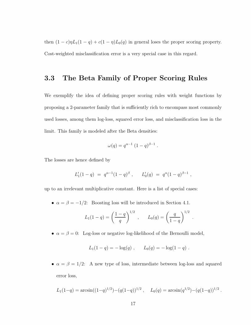
3.1 Loss functions L0(q) and weight functions ω(q) for various values of
α = β: exponential loss (α = −1/2), log-loss (α = 0), squared error
loss (α = 1), misclassification error (α =∞). These are scaled to pass
through 1 at q = 0.5. Also shown are α = 4, 20 and 100 scaled to show
convergence to the step function. . . . . . . . . . . . . . . . . . . . . . 19
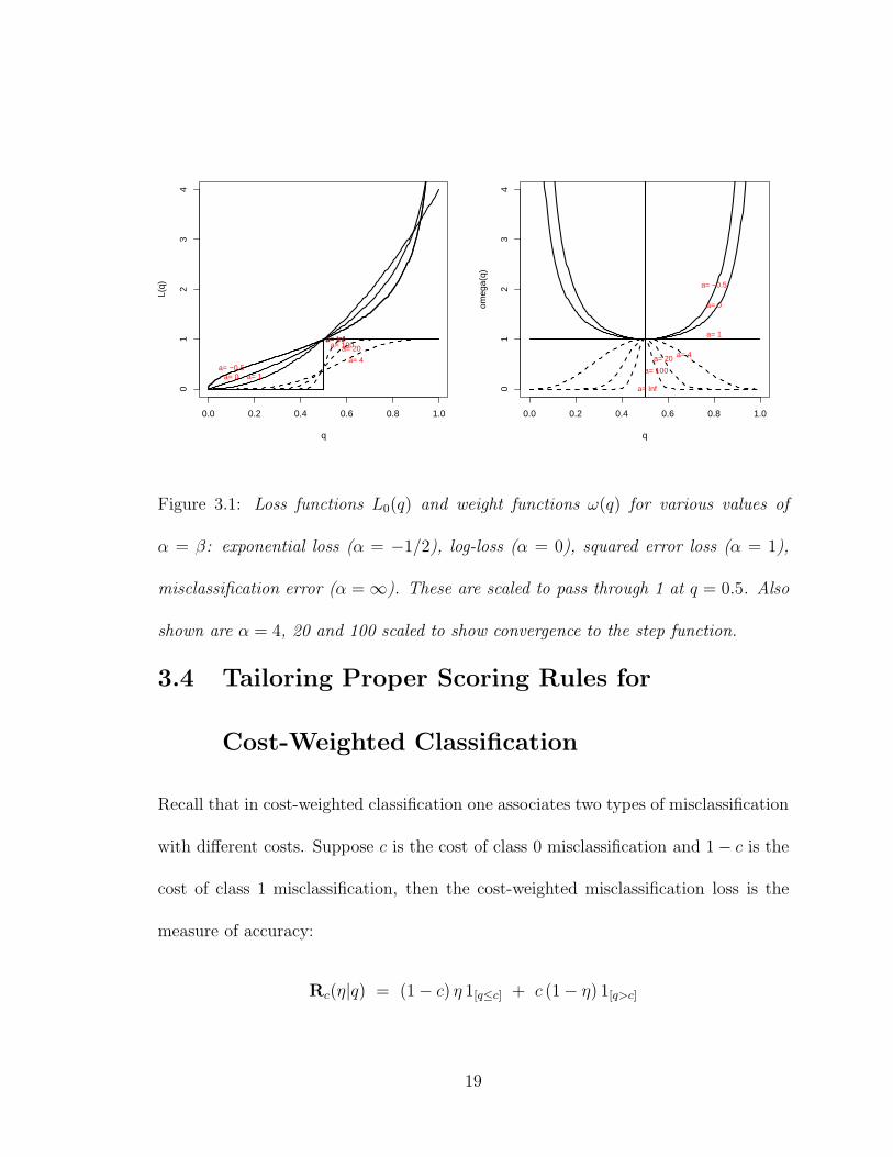
3.2 Loss functions L0(q) and weight functions ω(q) for various values of
α/β = 3/7, and c = 0.3: Shown are α = 2, 3 ,6 and 24 scaled to
show convergence to the step function. . . . . . . . . . . . . . . . . . 20
ix

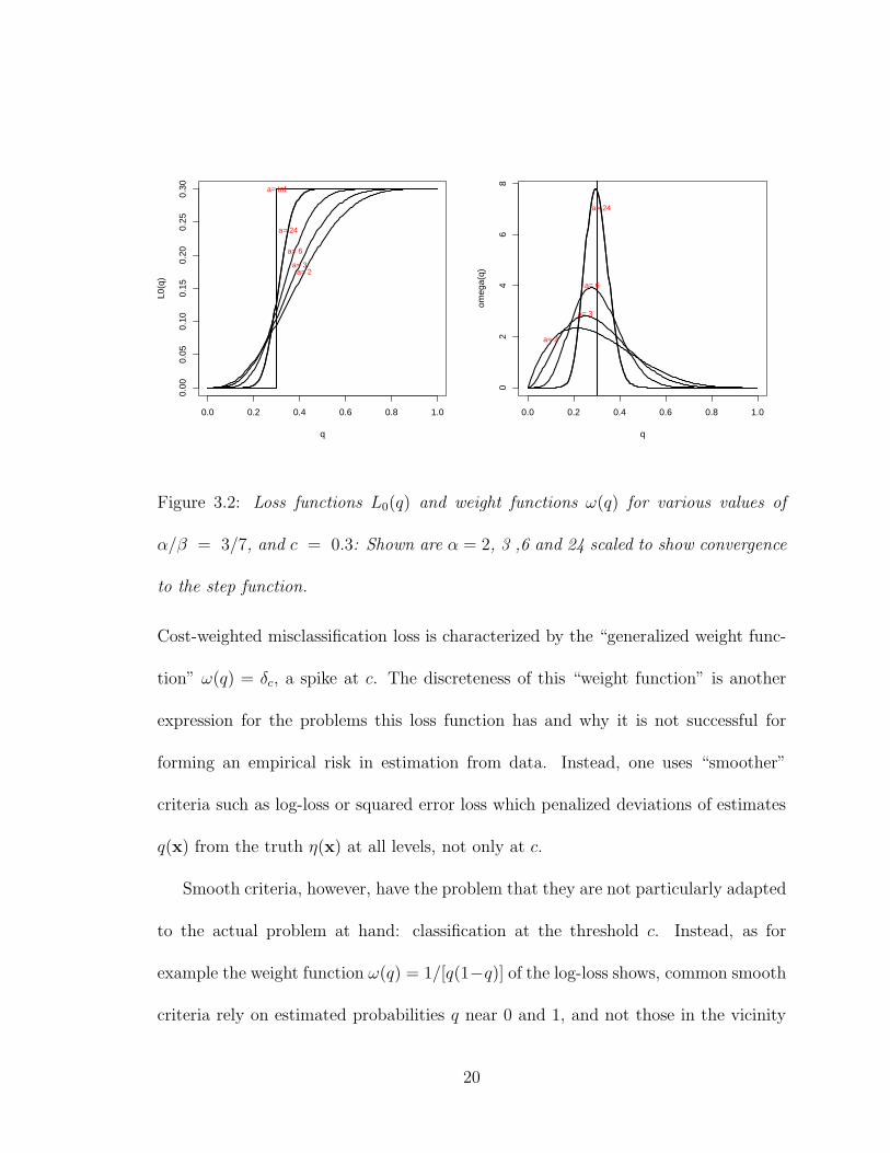
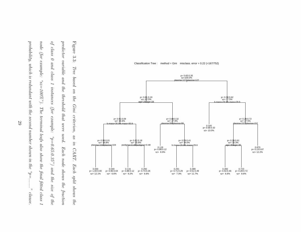
3.3 Tree based on the Gini criterion, as in CART. Each split shows the pre-
dictor variable and the threshold that were used. Each node shows the
fraction of class 0 and class 1 instances (for example: “p=0.65:0.35”)
and the size of the node (for example: “sz=100%”). The terminal leafs
also show the final fitted class 1 probability, which is redundant with
the second number shown in the “p=.......” clause. . . . . . . . . . . . 29
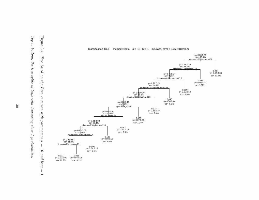
3.4 Tree based on the Beta criterion with parameters α = 16 and beta = 1.
Top to bottom, the tree splits of leafs with decreasing class 1 probabilities. 30
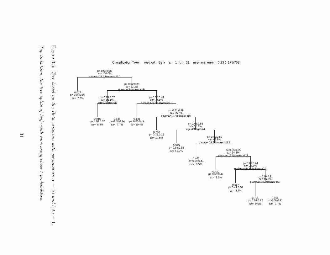
3.5 Tree based on the Beta criterion with parameters α = 16 and beta = 1.
Top to bottom, the tree splits of leafs with increasing class 1 probabilities. 31
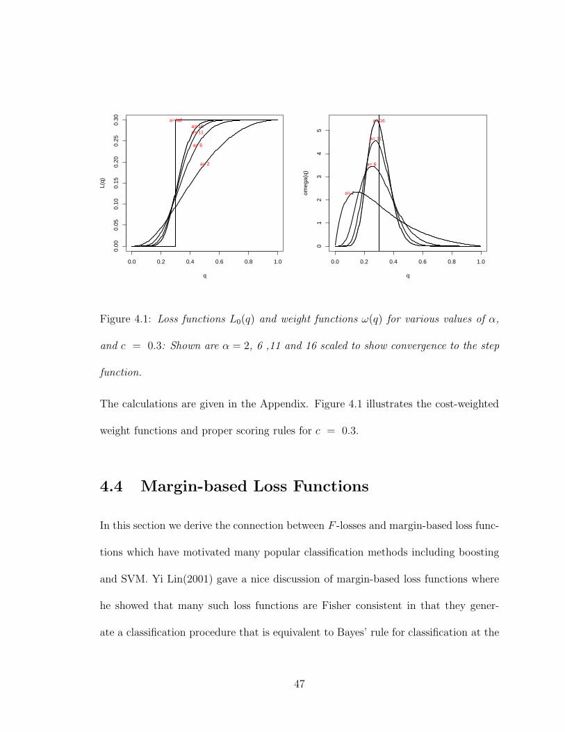
4.1 Loss functions L0(q) and weight functions ω(q) for various values of
α, and c = 0.3: Shown are α = 2, 6 ,11 and 16 scaled to show
convergence to the step function. . . . . . . . . . . . . . . . . . . . . . 47
x

7.1 Hand and Vinciotti’s Artificial Data: The class probability function
η(x) has the shape of a smooth spiral ramp on the unit square with axis
at the origin. The bold line marked “0.3 log” shows a linear logistic fit
thresholded at c = 0.3. The second bold line, marked “0.3 beta”, shows
a thresholded linear fit corresponding to a proper scoring rule in the
Beta family with parameters α = 6 and β = 14. The last bold line,
marked ”0.3 cw beta”, shows thresholded linear fit corresponding to
an cost-weighted F -loss derived from the Beta family with parameters
α = 4 and β = 4. . . . . . . . . . . . . . . . . . . . . . . . . . . . . . 69
7.2 A variation of Hand and Vinciotti’s Artificial Data with unbalanced
classes: The class 1 probability η(x) has the shape of a smooth spiral
ramp with axis at the origin. Shown are estimated contours of the
levels 0.3, 0.5 and 0.7. The blue lines show log-loss estimates (logistic
regression), the red lines Beta tailored estimates, and the magenta lines
cost-weighted tailored estimated, with tailoring for the respective levels. 70
7.3 The Pima Indian Diabetes Data, BODY against PLASMA. The colored
lines show the probability contours estimated with logistic regression
(blue), Beta tailoring (black), and cost-weighted tailoring (red). . . . . 72
7.4 The Pima Indian Diabetes Data, BODY against PLASMA. The high-
lights represent slices with near-constant q (c − ǫ ≤ q1 ≤ c + ǫ). The
values of q in the slices increase left to right and top to bottom. Open
squares: no diabetes (class 0), filled circles: diabetes (class 1). . . . . 73
xi
7.5 German credit data: Graphical permutation tests for comparing the
test errors based on log-loss, Beta loss with α/β = c/(1− c), and cost-
weighted F -loss with c = 1/6. . . . . . . . . . . . . . . . . . . . . . . 77
7.6 Histogram of the estimated σ for Beta tailoring (upper panel) and esti-
mated α for cost-weighted tailoring (lower panel) for the German credit
data with c = 1/6. In the estimation of σ and α with optimization of
cross-validated cost-weighted error we constrained σ between 0.06 and
0.2 in 0.02 increments and α to {2, 3, 4, 5, 6, 8, 10, 12} with the corre-
sponding σ to {0.139,0.114,0.092,0.0887,0.081,0.070,0.063,0.057}. . . . 78
7.7 Log-loss, Beta loss and CW-Beta loss with stumps after 50 iterations:
estimated class boundaries at c = 0.3. The data are a variation of Hand
and Vinciotti’s Artificial Data, where the class probability function p(x)
has the shape of an ascending-descending smooth spiral ramp. . . . . . 86
7.8 Similar to Figure 7.7: Log-loss, Beta tailored and cost-weighted tailored
loss after 300 iterations. . . . . . . . . . . . . . . . . . . . . . . . . . 87
7.9 Cost-weighted misclassification test error for c = .3. Tailored losses
perform better than log-loss by about 2%, but there is a slight tendency
to overfit after about 50 iterations. . . . . . . . . . . . . . . . . . . . 89
7.10 Similar to Figure 7.7: Log-loss, Beta tailored and cost-weighted tailored
loss with trees of depth three after 10 iterations. . . . . . . . . . 90
xii

7.11 Boosting with trees of depth three to the artificial data: The picture
shows the cost-weighted misclassification loss for c = .3 on test sets.
There is no significant difference between log-loss and tailored losses,
and they all tend to overfit quickly. . . . . . . . . . . . . . . . . . . . 91
7.12 German Credit Data: The frames show the cost-weighted misclassifi-
cation loss on holdout sets for c = 1/6.
Left panel: optimal choice of σ at 20 iterations; Right panel: at 200
iterations.
Black: log-loss; Blue: Beta tailored loss; Red: cost-weighted tailored
loss.
Recall, however, that linear regression with tailored loss performs better
than boosting (Table 7.4). . . . . . . . . . . . . . . . . . . . . . . . . 92
7.13 Adult Income Data: The three frames show the cost-weighted misclassi-
fication losses on the test set for c = .2, .5 and .8, respectively. Tailored
losses achieve better misclassification loss than log-loss during 300 it-
erations. The two types of tailoring are virtually indistinguishable.
Black: log-loss; Blue: Beta tailored loss; Red: cost-weighted tailored loss. 93
xiii
Chapter 1
Introduction
We consider predictor-response data with a binary response y representing the ob-
servation of classes y = 1 and y = 0. Such data are thought of as realizations of a
Bernoulli random variable Y with η = P [Y = 1] and 1− η = P [Y = 0]. The class 1
probability η is interpreted as a function of predictors x: η = η(x). If the predictors
are realizations of a random vector X, then η(x) is the conditional probability given
x: η(x) = P [Y = 1|X = x]. Of interest are two types of problems:
• Classification: Estimate a region in predictor space in which class 1 is observed
with the greatest possible majority. This amounts to estimating a region of the
form η(x) > c.
• Class probability estimation: Approximate η(x) as well as possible by fitting a
model q(x,b) (b = parameters to be estimated).
1

Of the two problems, classification is prevalent in machine learning (where it is some-
times called “concept learning”, betraying its origin in AI), whereas class probability
estimation is prevalent in statistics (often in the form of logistic regression).
The classification problem is peculiar in that estimation of a class 1 region requires
two kinds of criteria:
• The primary criterion of interest: misclassification rate. This is an intrinsically
unstable criterion for estimating models, a fact that necessitates the use of
• auxiliary criteria for estimation, such as the Bernoulli likelihood used in logistic
regression, and the exponential loss used in the boosting literature. These are
just estimation devices and not of primary interest.
The auxiliary criteria of classification are, however, the primary criteria of class prob-
ability estimation.
We describe two universes of loss functions that can be used as auxiliary criteria
in classification and as primary criteria in class probability estimation:
• One universe consists of loss functions that estimate probabilities consistently
or “properly”, whence they are called “proper scoring rules”. An example is
the negative log-likelihood of the Bernoulli model, also called Kullback-Leibler
information, log-loss, or cross-entropy (we use “log-loss” throughout).
• The other universe of loss functions is best characterized as producing estimators
that are “distorted” or uncalibrated. Why would one need such loss functions?
The reason is the same as in logistic regression where we model a “distortion”
2
of the probabilities, namely, the logit. We call such “distorted” loss functions
“F -losses” because their domains are scales to which functions (models) are
fitted. An example is the exponential loss used in boosting.
These two universes of loss functions allow us to address a peculiarity of classi-
fication: if a classification region is of the form q(x,b) > c, it is irrelevant for the
performance in terms of misclassification rate whether q(x,b) fits the true η(x) well,
as long as q(x,b) > c and η(x) > c agree well enough. That is, the classifier does not
suffer if q(x,b) is biased vis-a-vis η(x) as long as q(x,b) and η(x) are mostly on the
same side of c. It can therefore happen that a fairly inaccurate model yields quite ac-
curate classification. In order to take advantage of this possibility, one should choose
a loss function that is closer to misclassification rate than log-loss and exponential
loss. Squared error loss is more promising in that regard, but better choices of loss
functions can be found, in particular if misclassification cost is not equal for the two
classes.
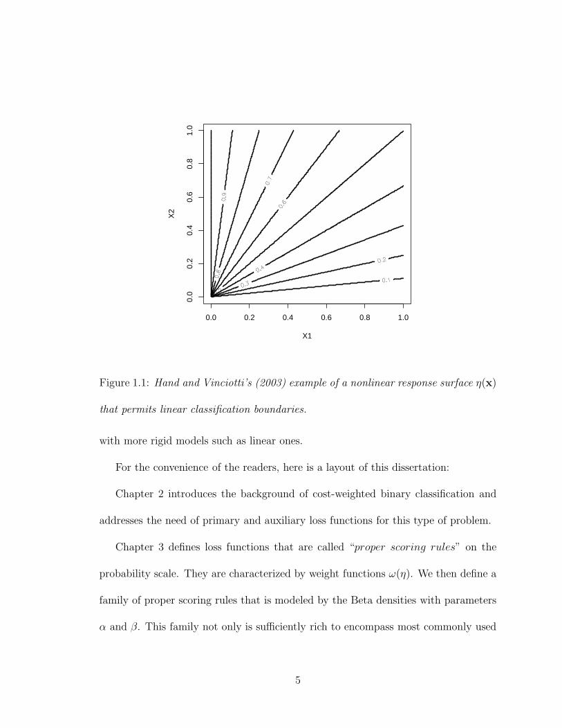
The discrepancy between class probability estimation and classification has re-
cently been illustrated by Hand and Vinciotti (2003) with a striking artificial exam-
ple. It demonstrates how good classification can occur even in the absence of good
class probability estimation. The example, shown in Figure 1.1, consists of a function
η(x) that is a rule surface, meaning that all the level lines are linear yet the function
is nonlinear. If we consider the class of linear functions, possibly passed through a
nonlinear link function such as the logistic, we will find that they are insufficient for
3

fitting this surface globally on its domain because the level lines of linear functions
as well as their nonlinear transforms are parallel to each other. Yet, for each level
0 < c < 1 one can find a linear function that describes the level line η(x) = c per-
fectly. This linear function will be unable to fit η(x) globally, hence in order to find
it one has to be able to ignore or at least downweight those training data for which
η(x) is far from c, the level of interest. Hand and Vinciotti (2003) have shown how
such downweighting can be done algorithmically, but their suggestion of a modified
likelihood (their Equation (2)) is rather tentative. We show how reweighting follows
as a direct consequence of the choice of proper scoring rule, and we also introduce
techniques for “tailoring” proper scoring rules for this purpose. —On the side we
note that we will show in an exercise of exploratory data analysis that Hand and
Vinciotti’s (2003) scenario approximately holds in the case of the well-known Pima
Indians Diabetes data from the UCI Machine Learning Repository (2003).
As a second application of the freedom of choice of loss function, we show how
criteria for tree-based classification can be “tailored” if the interest is in small or large
class probabilities. This exercise will produce highly interpretable trees that vastly
more expressive than the usual trees grown with the Gini index (CART, Breiman et
al. 1984) or entropy (e.g.: C4.5, Quinlan 1993; S language, Clark and Pregibon 1992).
Combining tailored losses with flexible non-parametric fits such as boosting mod-
els does not achieve a similarly strong benefit as in linear models. We show empirically
that as the complexity of the functional classes increases, the effect of tailoring be-
comes less significant. Thus we conclude that proper scoring rules are best combined
4
X1
X2
0.0 0.2 0.4 0.6 0.8 1.0
0.0
0.2
0.4
0.6
0.8
1.0
Figure 1.1: Hand and Vinciotti’s (2003) example of a nonlinear response surface η(x)
that permits linear classification boundaries.
with more rigid models such as linear ones.
For the convenience of the readers, here is a layout of this dissertation:
Chapter 2 introduces the background of cost-weighted binary classification and
addresses the need of primary and auxiliary loss functions for this type of problem.
Chapter 3 defines loss functions that are called “proper scoring rules” on the
probability scale. They are characterized by weight functions ω(η). We then define a
family of proper scoring rules that is modeled by the Beta densities with parameters
α and β. This family not only is sufficiently rich to encompass most commonly used
5

losses but can also be tailored for the purposes of cost-weighted classification.
Chapter 4 defines a larger class of loss functions than proper scoring rules that
we call “F − losses”. They are compositions of (inverse) link functions and proper
scoring rules. They can also be regarded as “uncalibrated” proper scoring rules in the
sense that the estimated values are not probability estimates, but can be calibrated
to produce probability estimates by applying a monotone transformation. We then
show that F -losses are closed under cost-weighting, thus can also be tailored for the
purposes of cost-weighted classification.
Chapters 5 and 6 deal with optimization of proper scoring rules and F -losses. In
Chapter 5 we generalize the IRLS algorithm to arbitrary proper scoring rules and F -
losses for linear models. In Chapter 6 we generalize stagewise fitting of additive models
(=“boosting” in Friedman et al.’s (2000) interpretation) to arbitrary proper scoring
rules and F -losses. In Chapter 7, we illustrate the application of such algorithms to
artificial and real world data sets.
6
Chapter 2
Two-Class Cost-Weighted
Classification
2.1 Cost-Weighting and Quantile Classification
In a two-class classification problem, one observes data (X, Y ), where X is predictor
or feature vector, Y is a binary response which is labeled 0 and 1. The observed
Y is regarded as a realization of a binary random variable following a Bernoulli
distribution. A problem of interest is to predict or classify future values of Y from the
information that the feature X contains. This amounts to the problem of dividing the
predictor space into two regions and classifying a case as 1 or 0 according to which
region the associated value of feature X falls in. Theoretically, the best (Bayes)
classification regions for assignment to class 1 are of the form {x | η(x) > c}, where
as before η(x) = P [Y = 1|x].
7
The determination of the threshold c is related to how much we weight the relative
cost of the two types of misclassification: misclassifying Y = 1 as 0 and Y = 0 as
1, respectively. In medical contexts, for example, a false negative (missing a disease)
is usually more severe than a false positive (falsely detecting a disease). If the cost
for class 1 misclassification is c1 and the cost for class 0 misclassification is c0, then
according to Bayes rule the optimal choice of c is c = c0/(c0 + c1). Without loss of
generality, one can always normalize the sum of c0 and c1 to 1: c0 + c1 = 1. The
threshold c = c0 is then the cost of class 0 misclassification. In those contexts where
costs are not mentioned, equal cost of misclassification is assumed, that is, c = 0.5.
Bayes rule is optimal in the sense of minimizing the cost of misclassification: the
expected costs of classifying as 1 and 0 are, respectively, c(1− η(x)) and (1− c)η(x).
Hence optimal classification as 1 is for c(1 − η(x)) < (1 − c)η(x) or, equivalently,
c < η(x). Thus, classification with normalized cost weight c is equivalent to “quantile
classification” at the quantile c.
In reality the posterior probability η(x) is unknown and has to be estimated from
the data. By convention, we use q(x) to denote an estimate of η(x). Therefore, one
uses an estimated classification region q(x) > c to approximate the true Bayes region
η(x) > c.
8
2.2 Cost-Weighting and Change of Baseline
A frequent confusion in classification concerns the roles of cost-weighting and change
of baseline frequencies of the two classes. For the convenience of the reader we show
how a baseline change affects the cost-weights or quantiles c (see, e.g., Elkan (2001)).
We use the following notation:
η(x) = P [Y = 1| x ] ,
π = P [Y = 1]
f1(x) = P [ x |Y = 1] ,
f0(x) = P [ x |Y = 0],
which are, respectively, the conditional probability of Y = 1 given X = x, the
unconditional (marginal/prior/baseline) probability of Y = 1, and the conditional
densities of X = x given Y = 1 and Y = 0. The densities f1/0(x) describe the
distributions of the two classes in predictor space. The joint distribution of (X, Y ) is
given by
η(y = 1, x) = f1(x) π , η(y = 0, x) = f0(x) π ,
and hence the conditional distribution of Y = 1 given X = x is
η(x) =f1(x) π
f1(x) π + f0(x) (1− π),
which is just Bayes theorem. Equivalently we have
η(x)
1− η(x)/
π
1− π=
f1(x)
f0(x). (2.1)
9
We then compare this situation with another one that differs only in the mix of class
labels, π∗ and 1 − π∗, as opposed to π and 1 − π. Denote by η∗(x) the conditional
probability of Y = 1 given X = x under this new mix. From Equation (2.1) follows
that f1(x) and f0(x) are the same in both situations, hence
η∗(x)
1− η∗(x)/
π∗
1− π∗=
η(x)
1− η(x)/
π
1− π,
or, equivalently,
η∗(x) =kη
kη + (1− k)(1− η),
where
k =π∗
1−π∗
π∗
1−π∗+ π
1−π
=π∗(1− π)
π∗(1− π) + (1− π∗)π.
Obviously thresholds c on η(x) and c∗ on η∗(x) transform the same way:
c∗ =kc
kc + (1− k)(1− c),
so that η∗(x) > c∗ iff η(x) > c.
2.3 Cost-Weighted Misclassification Error Loss
Our goal is to find classification rules whose cost-weighted misclassification error for
given costs c and 1 − c is small. We assume that classification is performed by
thresholding an estimate q(x) of η(x): the estimated class is 1q(x)>c. We encounter
an error if Y = 1 and q(x) ≤ c, or if Y = 0 and q(x) > c. Hence the cost-weighted
misclassification loss at x can be written as
L(Y |q(x)) = (1− c)Y 1[q(x)≤c] + c(1− Y )1[q(x)>c] .
10
When the costs of the two types of misclassification are the same, c = 1− c = .5, this
is up to a factor 1/2 the plain misclassification error:
L(Y |q(x)) = 0.5 ·(
Y 1[q(x)≤0.5] + (1− Y )1[q(x)>0.5]
)
At the population level, the conditional expected misclassification loss is:
EY |X=x L(Y |q(x)) = (1− c) η(x)1[q(x)≤c] + c (1− η(x))1[q(x)>c]
This is the expected loss associated with classification for a given value of X. Uncon-
ditionally, the cost-weighted misclassification loss or risk is:
EY,X (L(Y |q(X))) = (1− c) EX[ η(X)1[q(X)≤c]] + c EX[(1− η(X))1[q(X)>c]]
One would like to find estimators q(x) that perform well in the sense that they produce
a small risk. There is, however, a problem: misclassification loss is a crude measure
and does not distinguish between class 1 probability estimates q(x) as long as they
are on the same side of c. Hence optimal estimators q(x) are highly non-unique. In
many application one can make an argument that one would like q(x) to be a good
estimator of η(x), not just q(x) > c to be a good estimator of η(x) > c. This is the
case when the cost c is not precisely defined, or as in some marketing application
when potential customers need to be prioritized for marketing campaigns according
to their estimated probability of taking a product.
There is yet another problem with misclassification error: It is possible that two
estimators have the same misclassification error yet of them is preferable to the human
11
expert. For example, consider the following two pairs or misclassification counts:
ActualClass 1
Class 0
∗ 0
30 ∗
∗ 15
15 ∗
Both situations have the same unweighted misclassification error, yet they differ
strongly. It may help to consider the cost-weighted loss for each cost ratio: for the first
table it is 30·c+0·(1−c) = 30c, for the second table it is 15·c+15·(1−c) = 15. Thus,
if there is a potential of considering a class-0 cost c less than 0.5, one would clearly
prefer the first table, otherwise the second. As we will see, the criteria introduced
below will always prefer the first table over the second.
2.4 Some Common Losses
In Section 2.3 we illustrated some problems with misclassification loss. These prob-
lems arise from the crude nature of the loss function, one prefers to optimize over loss
functions with greater discriminatory properties. We give two standard examples:
Example 1. In logistic regression, one uses log-loss, (equivalently: Kullback-
Leibler loss, cross-entropy, or the negative log-likelihood of the Bernoulli model):
L(y|q) = −y log(q)− (1− y) log(1− q)
with the corresponding expected loss
R(η|q) = −η log(q)− (1− η) log(1− q)
12
Example 2. Squared error loss
L(y|q) = (y − q)2 = y(1− q)2 + (1− y)q2 ,
where the second equality holds because y takes only the values 0 and 1. The expected
squared error loss is
R(η|q) = η(1− q)2 + (1− η)q2 .
These two loss functions are smooth and they both produce particular solutions
of optimal estimates q. Moreover, one can quickly check that the optimal estimate
q is actually achieved at the true posterior probability η when minimizing the ex-
pected losses. Loss functions L(y|q) with this property have been known in subjective
probability as “proper scoring rules”. (See Garthwaite, Kadane and O’Hagan (2005,
Sec. 4.3) for recent work in this area.) There they are used to judge the quality of
probability forecasts by experts, whereas here they are used to judge the fit of class
probability estimators. Proper scoring rules form a natural universe of loss functions
for use as criteria for class probability estimation and classification.
13
Chapter 3
Proper Scoring Rules
3.1 Definition and Examples of Proper Scoring Rules
Definition: If an expected loss R(η|q) = ηL1(1−q)+(1−η)L0(q) is minimized w.r.t.
q by q = η ∀η ∈ (0, 1), we call the loss function a ”proper scoring rule”. If moreover
the minimum is unique, we call it a ”strictly proper scoring rule”.
According to the definition, we can easily see that the two examples in Section 2.4
are actually strictly proper scoring rules.
• For the expected log-loss, we have the first order stationarity condition
−η
q−
1− η
1− q= 0
which has the unique solution q = η.
• For the expected squared error loss, we have the first order stationarity condition
14
−2η(1− q) + 2(1− η)q = 0
which has the unique solution q = η.
It is also easy to see that misclassification loss is a proper scoring rule yet not
strict since the optimal solution q is not unique: any q that falls to the right side of
the true classification boundary η = c is considered optimal.
3.2 Characterizing Proper Scoring Rules
In this section we give a characterization of proper scoring rules that goes back to Shu-
ford, Albert, Massengill (1966), Savage (1971) and in its most general form Schervish
(1989).
We write the stationarity condition under which classification loss functions L(y|q)
form proper scoring rules, and we will characterize them in terms of “weight func-
tions”. Writing the loss function as
L(y|q) = yL1(1− q) + (1− y)L0(q)
we have:
Proposition 1: Let L1(·) and L0(·) be monotone increasing functions. If L1(·) and
L0(·) are differentiable, then L(y|q) forms a proper scoring rule iff
L′1(1− q) = ω(q)(1− q), L′
0(q) = ω(q)q (3.1)
15

If ω(q) is strictly positive on (0, 1), then the proper scoring rule is strict.
The proof follows immediately from the stationarity condition,
0 =∂
∂q
∣
∣
∣
∣
q=η
L(η|q) = − η L′1(1− η) + (1− η) L′
0(η) .
This entails
L′1(1− q)
1− q=
L′0(q)
q,
which defines the weight function ω(q).
Proposition 1 reveals the possibility of constructing new proper scoring rules by
choosing appropriate weight functions ω(q). Here are two standard examples of such
choices:
• Log-loss:
ω(q) =1
q(1− q)
• Squared error loss:
ω(q) = 1
Misclassification loss does not fit in this framework because its losses L0(q) =
c 1[q>c] and L1(1− q) = (1− c) 1[q≤c] are not smooth. Yet there exists an extension of
the above proposition that allows us to write down a “generalized weight function”:
ω(q) = δc(dq)
We conclude with the observation that in general proper scoring rules do not allow
cost-weighting. That is, if ηL1(1 − q) + (1 − η)L0(q) defines a proper scoring rule,
16
then (1 − c)ηL1(1 − q) + c(1 − η)L0(q) in general loses the proper scoring property.
Cost-weighted misclassification error is a very special case in this regard.
3.3 The Beta Family of Proper Scoring Rules
We exemplify the idea of defining proper scoring rules with weight functions by
proposing a 2-parameter family that is sufficiently rich to encompass most commonly
used losses, among them log-loss, squared error loss, and misclassification loss in the
limit. This family is modeled after the Beta densities:
ω(q) = qα−1 (1− q)β−1 .
The losses are hence defined by
L′1(1− q) = qα−1(1− q)β , L′
0(q) = qα(1− q)β−1 ,
up to an irrelevant multiplicative constant. Here is a list of special cases:
• α = β = −1/2: Boosting loss will be introduced in Section 4.1.
L1(1− q) =
(
1− q
q
)1/2
, L0(q) =
(
q
1− q
)1/2
.
• α = β = 0: Log-loss or negative log-likelihood of the Bernoulli model,
L1(1− q) = − log(q) , L0(q) = − log(1− q) .
• α = β = 1/2: A new type of loss, intermediate between log-loss and squared
error loss,
L1(1−q) = arcsin((1−q)1/2)−(q(1−q))1/2 , L0(q) = arcsin(q1/2)−(q(1−q))1/2 .
17

• α = β = 1: Squared error loss,
L1(1− q) = (1− q)2 , L0(q) = q2 .
• α = β = 2: A new loss closer to misclassification than squared error loss,
L1(1− q) =1
3(1− q)3 −
1
4(1− q)4 , L0(q) =
1
3q3 −
1
4q4 .
• α = β →∞: The misclassification error rate,
L1(1− q) = 1[1−q>1/2] , L0(q) = 1[q≥1/2] .
Values of α and β that are integer multiples of 1/2 permit closed formulas for L1
and L0. For other values one needs a numeric implementation of the incomplete Beta
function.
Figure 3.1 and Figures 3.2 show proper scoring rules derived from the Beta family
with various parameters α and β for different costs.
18
0.0 0.2 0.4 0.6 0.8 1.0
01
23
4
q
L(q)
a= −0.5a= 0 a= 1
a= 4
a= 20a= 100a= Infa= Inf
0.0 0.2 0.4 0.6 0.8 1.0
01
23
4
q
omeg
a(q)
a= −0.5
a= 0
a= 1
a= 4a= 20
a= 100
a= Inf
Figure 3.1: Loss functions L0(q) and weight functions ω(q) for various values of
α = β: exponential loss (α = −1/2), log-loss (α = 0), squared error loss (α = 1),
misclassification error (α =∞). These are scaled to pass through 1 at q = 0.5. Also
shown are α = 4, 20 and 100 scaled to show convergence to the step function.
3.4 Tailoring Proper Scoring Rules for
Cost-Weighted Classification
Recall that in cost-weighted classification one associates two types of misclassification
with different costs. Suppose c is the cost of class 0 misclassification and 1− c is the
cost of class 1 misclassification, then the cost-weighted misclassification loss is the
measure of accuracy:
Rc(η|q) = (1− c) η 1[q≤c] + c (1− η) 1[q>c]
19
0.0 0.2 0.4 0.6 0.8 1.0
0.00
0.05
0.10
0.15
0.20
0.25
0.30
q
L0(q
)
a= 24
a= 6
a= 3a= 2
a= Inf
0.0 0.2 0.4 0.6 0.8 1.0
02
46
8
q
omeg
a(q)
a= 24
a= 6
a= 3
a= 2
Figure 3.2: Loss functions L0(q) and weight functions ω(q) for various values of
α/β = 3/7, and c = 0.3: Shown are α = 2, 3 ,6 and 24 scaled to show convergence
to the step function.
Cost-weighted misclassification loss is characterized by the “generalized weight func-
tion” ω(q) = δc, a spike at c. The discreteness of this “weight function” is another
expression for the problems this loss function has and why it is not successful for
forming an empirical risk in estimation from data. Instead, one uses “smoother”
criteria such as log-loss or squared error loss which penalized deviations of estimates
q(x) from the truth η(x) at all levels, not only at c.
Smooth criteria, however, have the problem that they are not particularly adapted
to the actual problem at hand: classification at the threshold c. Instead, as for
example the weight function ω(q) = 1/[q(1−q)] of the log-loss shows, common smooth
criteria rely on estimated probabilities q near 0 and 1, and not those in the vicinity
20

of c which is the locus of interest. This consideration motivates our examination of
continuous losses other than log-loss and squared error loss, losses that may be better
adapted to particular thresholds c of interest. Intuitively, we look for losses with
smooth weight functions that approximate the spike δc, or at least shift the mass of
ω(q) off-center to reflect the cost-weights c and 1− c.
With this road map, it is natural to turn to the Beta family of weight functions
because Beta distributions are sufficiently rich to approximate point masses δc at any
location 0 < c < 1. The Beta densities
ωα,β(q) =1
B(α, β)qα−1(1− q)β−1
converge to ω(q) = δc(q), for example, when
α, β →∞ , subject toα
β=
c
1− c.
For a proof note that the conditions force the expectation to µ = c while the variance
converges to zero:
• The expected value of q under a Beta distribution with parameters α and β is
µ =α
α + β,
which equals c if c/(1− c) = α/β.
• The variance is
σ2 =αβ
(α + β)2(α + β + 1)=
c(1− c)
α + β + 1,
which converges to zero if α, β →∞.
21
In a limiting sense, the ratio of the exponents, α/β, acts as a cost ratio for the classes.
One could also tailor in a slightly different way. Instead of matching the parame-
ters α and β to the mean, one could match to the mode:
c = qmode =α− 1
α + β − 2
With either mean or mode matching, we obtain weak convergence ω(q)dq → δc(dq).
The above construction has obvious methodological implications for logistic re-
gression and also, as will be shown later, for boosting: log-loss and exponential loss,
which they use, respectively, can be replaced with the proper scoring rules generated
by the above weight functions ωα,β(q). In doing so we may be able to achieve im-
proved classification for particular cost ratios or class-probability thresholds when the
fitted model is biased but adequate for describing classification boundaries individu-
ally. The appropriate degree of peakedness of the weight function can be estimated
from the data. See Chapter 7 for examples.
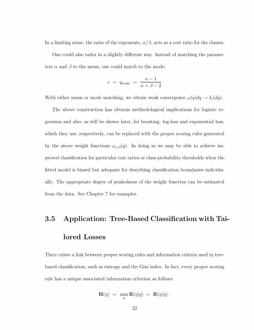
3.5 Application: Tree-Based Classification with Tai-
lored Losses
There exists a link between proper scoring rules and information criteria used in tree-
based classification, such as entropy and the Gini index. In fact, every proper scoring
rule has a unique associated information criterion as follows:
H(η) = minq
R(η|q) = R(η|η) .
22
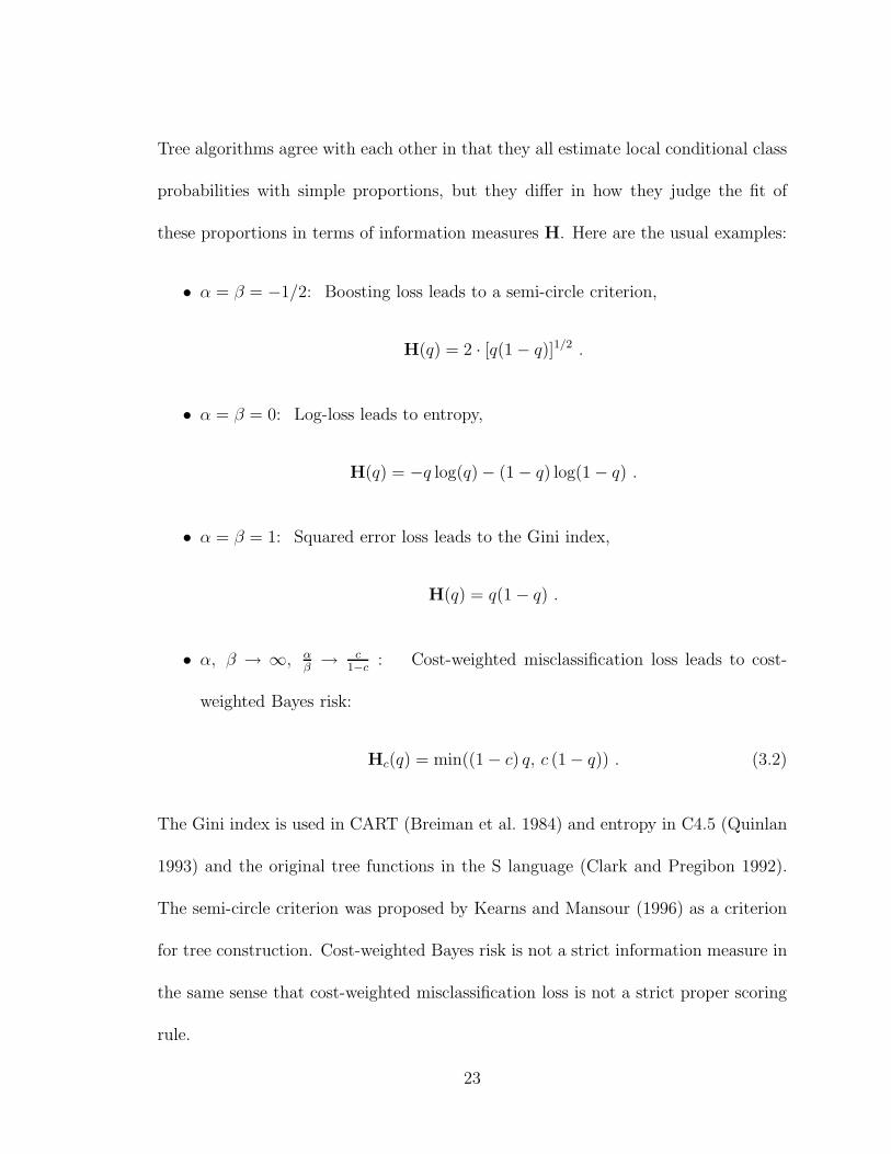
Tree algorithms agree with each other in that they all estimate local conditional class
probabilities with simple proportions, but they differ in how they judge the fit of
these proportions in terms of information measures H. Here are the usual examples:
• α = β = −1/2: Boosting loss leads to a semi-circle criterion,
H(q) = 2 · [q(1− q)]1/2 .
• α = β = 0: Log-loss leads to entropy,
H(q) = −q log(q)− (1− q) log(1− q) .
• α = β = 1: Squared error loss leads to the Gini index,
H(q) = q(1− q) .
• α, β → ∞, αβ→ c
1−c: Cost-weighted misclassification loss leads to cost-
weighted Bayes risk:
Hc(q) = min((1− c) q, c (1− q)) . (3.2)
The Gini index is used in CART (Breiman et al. 1984) and entropy in C4.5 (Quinlan
1993) and the original tree functions in the S language (Clark and Pregibon 1992).
The semi-circle criterion was proposed by Kearns and Mansour (1996) as a criterion
for tree construction. Cost-weighted Bayes risk is not a strict information measure in
the same sense that cost-weighted misclassification loss is not a strict proper scoring
rule.
23

The following proposition shows that every information measure determines es-
sentially a unique proper scoring rule, modulo some arbitrary choices for those q
for which the function H(q) does not have a unique tangent, as for cost-weighted
misclassification losses at the location q = c.
Proposition: The information measure H(q) is the concave lower envelope of
its proper scoring rule R(η|q), with upper tangents η 7→ R(η|q). Conversely, if H(q)
is an arbitrary concave function, it determines a proper scoring rule R(η|q) which is
unique except at locations where there are multiple upper tangents, in which case any
of the tangents can be selected as part of the definition of the proper scoring rule.
Corollary: If H(q) is concave and smooth, its associated proper scoring rule is
L1(1− q) = H(q) + H′(q) (1− q) , L0(q) = H(q)−H′(q) q . (3.3)
For a proof, note that R(η|q) is affine in η and R(η|q) ≥ H(η), which makes
η 7→ R(η|q) an upper tangent for all q and hence H(q) the concave lower envelope.
Conversely, given a concave function H(q), there exist upper tangents at every q.
They are affine functions and can be written η 7→ η T1(q) + (1− η) T0(q), so one can
define L1(1− q) = T1(q) and L0(q) = T0(q). For the corollary, the upper tangent at
q is unique and can be written as an affine function η 7→ H′(q)(η− q) + H(q). Hence
R(η|q) = H′(q)(η− q)+H(q) defines the proper scoring rule: L1(1− q) = R(1|q) and
L0(q) = R(0|q).
24
Proposition: If H(q) is concave and sufficiently smooth, the weight function ω(q)
of the associated proper scoring rule is:
ω(q) = −H′′(q) . (3.4)
The proof is a simple calculation. The relation links concavity and non-negative
weights, as well as strict concavity and positive weights. The proposition indicates
that information measures with the same second derivative are equivalent. In other
words, information measures that differ only in an affine function are equivalent:
H(q) + C1 q + C0 (1 − q). This fact follows for all information measures, not only
smooth ones, from the equivalence of proper scoring rules that differ in two constants
only, L1(1− q) + C1 and L0(q) + C0.
Tailored classification trees: In light of these facts it is natural to apply the
tailoring ideas of Section 3.4 to information measures for tree-based classification. The
idea is again to put weight on the class probabilities that are of interest. “Weight”
is meant literally in terms of the weight function ω(q). In practice, areas of interest
are often the extremes with highest or lowest class probabilities. In the Pima Indians
diabetes data, for example, this may mean focusing on the cases with an estimated
probability of diabetes of 0.9 or greater. It would then be reasonable to use an
information measure derived from a weight function that puts most of its mass on
the right end of the interval (0,1). We will show experiments with weights that
are simple power functions of q. In terms of the Beta family of weights this could
mean using β = 1 and α > 1: ω(q) ∼ qα−1. An associated information measure is
25

H(q) ∼ −qα+1, but taking advantage of the indeterminacy of information measures
modulo affine functions, an equivalent but more pleasing choice is H(q) = (1− qα)q,
which is normalized such that H(0) = H(1) = 0.
The result of such an experiment for the Pima Indians Diabetes data (UCI ML
Database). Figure 3.5 shows a tree grown with the Gini index. The depth to which
it is grown and the quality of the fit is not of concern; instead, we focus on inter-
pretability. This tree shows the usual relative balance whereby most splits are not
more lopsided than about 1:2 in bucket size. Overall, interpretation is not easy, at
least in comparison to the trees shown in the following two figures. The latter were
obtained with information criteria from the Beta family. The tree in Figure 3.5 is
based on the parameters α = 16 and β = 1, which means a strong focus on large
class 1 probabilities (more correctly: class 1 frequencies). By contrast, Figure 3.5 is
based on α = 1 and β = 31, hence a strong focus on small class 1 probabilities.
The focus on the upper and the lower end of probabilities in these two trees
really amounts to prioritizing the splits from the bottom up and from the top down,
respectively. Accordingly, Figure 3.5 shows a highly unbalanced tree that peels off
small terminal leafs with low class 1 probability. As higher level terminal leafs peel
off the highest class 1 probability areas, subsequent terminal leafs must consequently
have ever lower class 1 probabilities. The result is a cascading tree that layers the
data as well as possible from highest to lowest class 1 probabilities. The dual effect is
seen in Figure 3.5: a layering of the data according to increasing class 1 probabilities.
26

While it may be true that the lopsided focus of the criterion is likely to lead to
suboptimal trees for standard prediction, cascading trees are vastly more powerful
in terms of interpretation: they permit, for example, the expression of dose-response
effects and generally of monotone relationships between predictors and response. For
example, both trees feature “plasma” as the single most frequent splitting variable
which seems to correlate positively with the probability of diabetes: as we descend the
trees and as the splitting values on “plasma” decrease in Figure 3.5 and increase in
Figure 3.5, the class 1 probabilities decrease and increase, respectively. In Figure 3.5
the variable “b.mass” asserts itself as the second most frequent predictors, and again
a positive relation with class 1 probabilities can be gleaned from the tree. Similarly,
Figure 3.5 exhibits positive dependences for “age” and “pedigree” as well.
A second aspect that helps the interpretation of cascading trees is the fact that
repeat appearances of the same predictors lower the complexity of the description
of low hanging leafs. For example, in Figure 3.5 the right most leaf at the bottom
with the highest class 1 probability q = 0.91 is of depth nine, yet it does not require
nine inequalities to describe it. Instead, the following four suffice: “plasma > 155”,
“pedigree > 0.3”, “b.mass > 29.9” and “age > 24”.
Interestingly the tree of Figure 3.5 that peels off low class 1 probabilities ends up
with a crisper high-probability leaf than the tree of Figure 3.5 whose greedy search
for high class 1 probabilities results only in an initial leaf with q = 0.86 characterized
by the single inequality “plasma > 166”.
27

We reiterate and summarize: the extreme focus on high or low class 1 probabilities
cannot be expected to perform well in terms of conventional prediction, but it may
have merit in producing trees with vastly greater interpretability.
The present approach to interpretable trees produces results that are similar to an
earlier proposal by Buja and Lee (2001). This latter approach is based on splitting
that maximizes the larger of the two class 1 probabilities. The advantage of the
tailored trees introduced here is that there actually exists a criterion that is being
minimized, and tree-performance can be measured in terms of this criterion.
28
|plasma<127/plasma>127
age<28/age>28
b.mass<30.9/b.mass>30.9
plasma<104/plasma>104 pedigree<0.48/pedigree>0.48
plasma<99/plasma>99
b.mass<29.6/b.mass>29.6
b.mass<29.9/b.mass>29.9
plasma<157/plasma>157
age<30/age>30
0.000 0.040 0.116 0.260
0.119
0.291 0.489
0.320
0.460 0.723
0.870
p= 1.00:0.00 p= 0.96:0.04 p= 0.88:0.12 p= 0.74:0.26
p= 0.88:0.12
p= 0.71:0.29 p= 0.51:0.49
p= 0.68:0.32
p= 0.54:0.46 p= 0.28:0.72
p= 0.13:0.87
sz= 12.1% sz= 6.6% sz= 9.2% sz= 6.6%
sz= 8.9%
sz= 7.3% sz= 11.7%
sz= 10.0%
sz= 6.6% sz= 8.6%
sz= 12.2%
p= 0.65:0.35
p= 0.81:0.19
p= 0.91:0.09
p= 0.99:0.01 p= 0.82:0.18
p= 0.68:0.32
p= 0.59:0.41
p= 0.38:0.62
p= 0.28:0.72
p= 0.39:0.61
sz=100.0%
sz= 62.5%
sz= 34.6%
sz= 18.8% sz= 15.8%
sz= 27.9%
sz= 19.0%
sz= 37.5%
sz= 27.5%
sz= 15.3%
Classification Tree : method = Gini misclass. error = 0.22 (=167/752)
Figu
re3.3:
Tree
based
on
the
Gin
icriterio
n,
as
inC
ART
.Each
split
shows
the
pred
ictor
varia
bleand
the
thresh
old
that
were
used
.Each
nod
esh
ows
the
fractio
n
of
class
0and
class
1in
stances
(for
exam
ple:
“p=
0.6
5:0
.35”)
and
the
sizeof
the
nod
e(fo
rexa
mple:
“sz=
100%
”).
The
termin
allea
fsalso
show
the
finalfitted
class
1
pro
bability,
which
isred
undantwith
the
second
num
bersh
own
inth
e“p=
.......”cla
use.
29
|plasma<166/plasma>166
plasma<143/plasma>143
b.mass<40.7/b.mass>40.7
pedigree<0.83/pedigree>0.83
plasma<130/plasma>130
age<39/age>39
age<30/age>30
plasma<118/plasma>118
pedigree<0.5/pedigree>0.5
b.mass<29/b.mass>29
0.011 0.065
0.160
0.196
0.262
0.326
0.373
0.440
0.500
0.598
0.861
p= 0.99:0.01 p= 0.94:0.06
p= 0.84:0.16
p= 0.80:0.20
p= 0.74:0.26
p= 0.67:0.33
p= 0.63:0.37
p= 0.56:0.44
p= 0.50:0.50
p= 0.40:0.60
p= 0.14:0.86
sz= 11.7% sz= 10.2%
sz= 6.6%
sz= 6.8%
sz= 8.6%
sz= 11.4%
sz= 7.8%
sz= 6.6%
sz= 6.6%
sz= 12.9%
sz= 10.5%
p= 0.65:0.35
p= 0.71:0.29
p= 0.76:0.24
p= 0.79:0.21
p= 0.81:0.19
p= 0.83:0.17
p= 0.88:0.12
p= 0.91:0.09
p= 0.93:0.07
p= 0.96:0.04
sz=100.0%
sz= 89.5%
sz= 76.6%
sz= 69.9%
sz= 63.3%
sz= 55.5%
sz= 44.0%
sz= 35.4%
sz= 28.6%
sz= 21.9%
Classification Tree : method = Beta a = 16 b = 1 misclass. error = 0.25 (=188/752)
Figu
re3.4:
Tree
based
on
the
Beta
criterion
with
para
meters
α=
16and
beta=
1.
Top
tobo
ttom
,th
etree
splits
oflea
fswith
decrea
sing
class
1pro
babilities.
30
|b.mass<23.2/b.mass>23.2
plasma<94/plasma>94
age<25/age>25 b.mass<26.3/b.mass>26.3
plasma<107/plasma>107
age<24/age>24
b.mass<29.9/b.mass>29.9
plasma<123/plasma>123
pedigree<0.3/pedigree>0.3
plasma<155/plasma>155
0.017
0.016 0.138 0.141
0.253
0.325
0.406
0.420
0.587
0.721 0.914
p= 0.98:0.02
p= 0.98:0.02 p= 0.86:0.14 p= 0.86:0.14
p= 0.75:0.25
p= 0.68:0.32
p= 0.59:0.41
p= 0.58:0.42
p= 0.41:0.59
p= 0.28:0.72 p= 0.09:0.91
sz= 7.8%
sz= 8.4% sz= 7.7% sz= 10.4%
sz= 12.6%
sz= 10.2%
sz= 8.5%
sz= 9.2%
sz= 8.4%
sz= 9.0% sz= 7.7%
p= 0.65:0.35
p= 0.62:0.38
p= 0.93:0.07 p= 0.56:0.44
p= 0.51:0.49
p= 0.45:0.55
p= 0.40:0.60
p= 0.35:0.65
p= 0.26:0.74
p= 0.19:0.81
sz=100.0%
sz= 92.2%
sz= 16.1% sz= 76.1%
sz= 65.7%
sz= 53.1%
sz= 42.8%
sz= 34.3%
sz= 25.1%
sz= 16.8%
Classification Tree : method = Beta a = 1 b = 31 misclass. error = 0.23 (=175/752)
Figu
re3.5:
Tree
based
on
the
Beta
criterion
with
para
meters
α=
16and
beta=
1.
Top
tobo
ttom
,th
etree
splits
oflea
fswith
increa
sing
class
1pro
babilities.
31

Chapter 4
F -losses: Compositions of Proper
Scoring Rules and Link Functions
We consider in this chapter a larger class of loss functions than proper scoring rules.
We call them F -losses for reasons that become clear below. There are two ways
of describing F -losses: The first way is to think of them as “uncalibrated” proper
scoring rules in the sense that the estimated values are not probability estimates,
but they can be calibrated to produce probability estimates by applying a monotone
transformation. We can also think of F -losses as the composition of (inverse) link
functions and proper scoring rules. This latter description will be our definition and
the former a result (Proposition 2).
32

4.1 Introducing F -losses
The constraint of probabilities to the 0-1 interval is inconvenient for modeling. If
one wanted, for example, to directly approximate probabilities with a linear model,
it would be difficult to bound the fit for those instances with extreme features. The
same problem occurs with any function class that has unbounded functions such
as polynomials and splines. The conflict between a desire for unbounded modeling
scales and the necessity of estimating probabilities that are bounded between 0 and
1 is overcome by the use of link functions.
We will refer to the “modeling scale” as “F -scale”. In a linear model we would
have F (x) =∑
βjx(j), and in an additive model F (x) =
∑
fi(x(j)). The use of the
letter F is standard in machine learning and associated statistical literature such as
FHT (2000).
Unfortunately, the transformation F 7→ q(F ) that maps F (x) to the probability
scale is by convention the inverse link function. We therefore have a need to use the
notation q 7→ F (q) for what is conventionally called the link function. This, however,
brings us into conflict with the notation for model fits x 7→ F (x). We will use both
notations and simply trust that the reader will be able to tell which is which from
the context. In summary, a model fit F (x) is passed through the inverse q = q(F ) of
a link function F = F (q) to arrive at a fitted probability q(F (x)).
Definition: An F -loss is defined as the composition of the inverse q(F ) = F−1(F )
of a continuous, strictly increasing (hence invertible) link function F (q) and a proper
33

scoring rule R(η|q):
R(η |F ) = R(η |q(F ))
An F -loss is called strict if its proper scoring rule is strict.
Remarks:
• All proper scoring rules are F -losses because the identity transformation quali-
fies as a link function. Note that the range of the link function is not required
to be all of the real line.
• If F (q) is a link function (continuous and strictly increasing), then by construc-
tion F (η) minimizes the F -loss: infF R(η|F ) = R(η|F (η)). If the F -loss is
strict, this is the unique minimizer.
• There exists a question of non-identifiability between link functions and models
because almost all models are closed under addition of constants. Therefore,
a model fit F (x) combined with a link function F (q) is equivalent to a model
fit F (x) + k combined with a link function F (q) + k. Both map x to the same
probability q. One can therefore fix the translation of the F -scale w.l.o.g. by
requiring, for example, F (1/2) = 0 or F (c) = 0. Such requirements agree with
the convention in machine learning that uses 0 as the classification boundary
({F (x) > 0} estimates class 1) and (2Y − 1)F as the “margin” or “signed
distance” from the boundary.
• We can leave it to convenience whether the end points 0 and 1 of the unit
34

intervals are part of the domain of the link function. If they are included in the
domain and the link function is unbounded, then ±∞ will have to be included
in the range.
We give some common examples and counter examples of F -losses for classification
problems.
Example 1. Logistic loss: log-loss combined with the logistic link
F (q) = logq
(1− q)
The link is symmetric about (1/2, 0). The inverse link is
q(F ) =1
1 + e−F
The resulting F -loss is
R(η|F ) = η log(1
1 + e−F) + (1− η) log(
1
1 + eF)
Example 2. Probit link and log-loss:
F (q) = Φ−1(q)
where Φ−1 is the inverse of the standard normal cumulative distribution function.It
is also symmetric about (1/2, 0). Then the inverse link is
q(F ) = Φ(F )
The resulting F -loss is
R(η|F ) = η log(Φ(F )) + (1− η) log(1− Φ(F ))
35
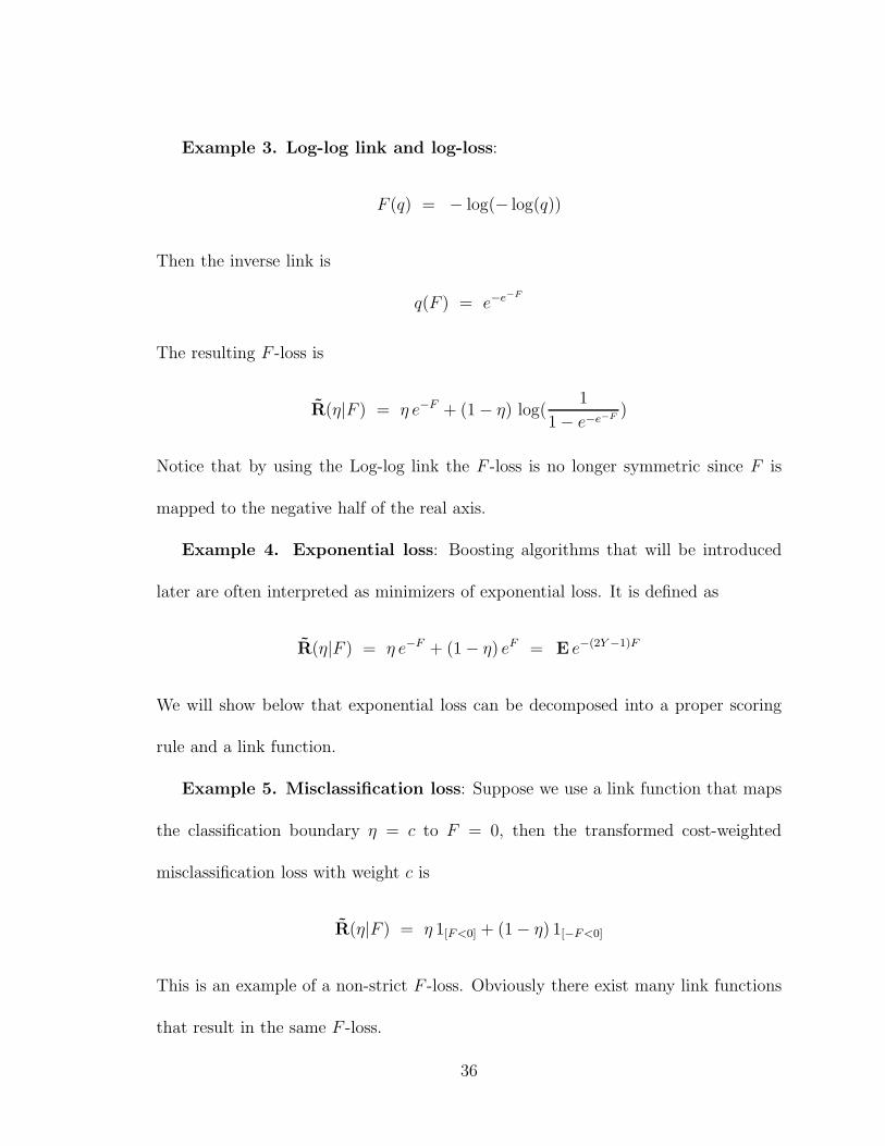
Example 3. Log-log link and log-loss:
F (q) = − log(− log(q))
Then the inverse link is
q(F ) = e−e−F
The resulting F -loss is
R(η|F ) = η e−F + (1− η) log(1
1− e−e−F)
Notice that by using the Log-log link the F -loss is no longer symmetric since F is
mapped to the negative half of the real axis.
Example 4. Exponential loss: Boosting algorithms that will be introduced
later are often interpreted as minimizers of exponential loss. It is defined as
R(η|F ) = η e−F + (1− η) eF = E e−(2Y −1)F
We will show below that exponential loss can be decomposed into a proper scoring
rule and a link function.
Example 5. Misclassification loss: Suppose we use a link function that maps
the classification boundary η = c to F = 0, then the transformed cost-weighted
misclassification loss with weight c is
R(η|F ) = η 1[F<0] + (1− η) 1[−F<0]
This is an example of a non-strict F -loss. Obviously there exist many link functions
that result in the same F -loss.
36
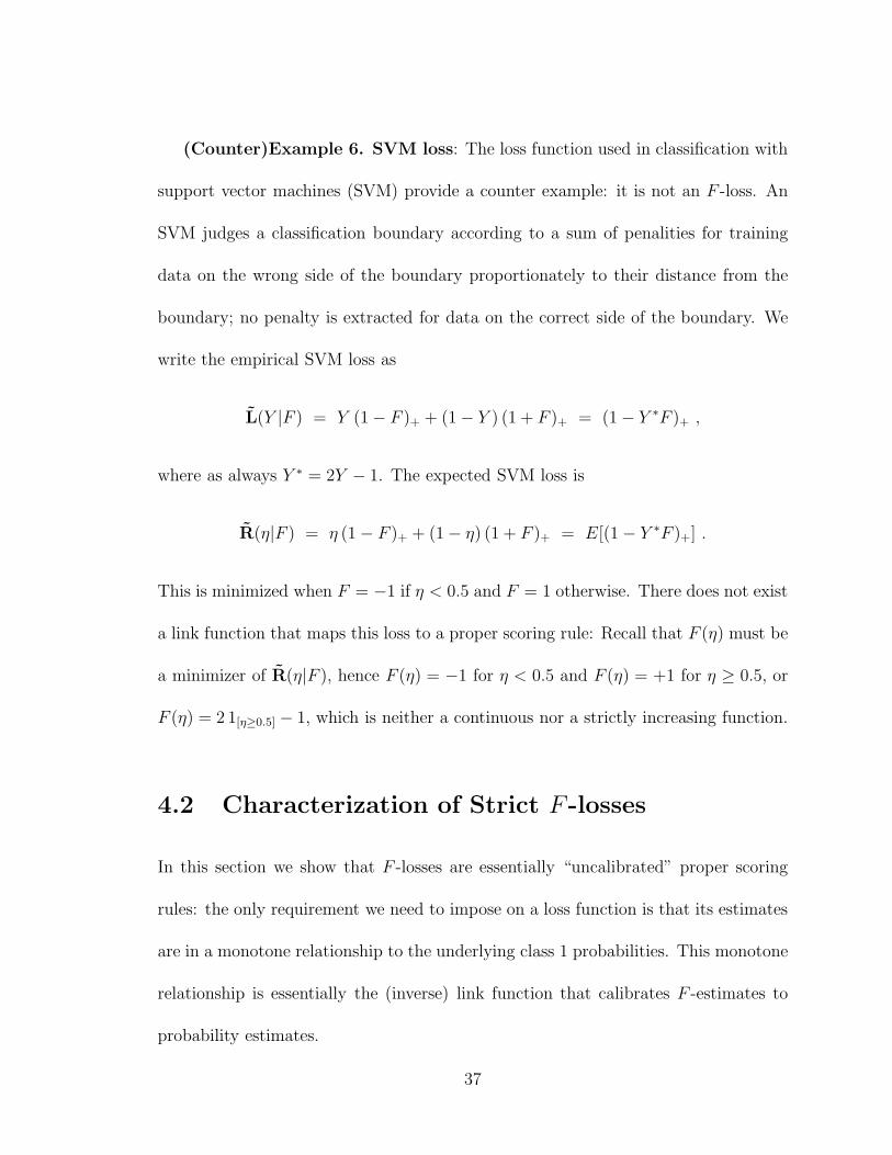
(Counter)Example 6. SVM loss: The loss function used in classification with
support vector machines (SVM) provide a counter example: it is not an F -loss. An
SVM judges a classification boundary according to a sum of penalities for training
data on the wrong side of the boundary proportionately to their distance from the
boundary; no penalty is extracted for data on the correct side of the boundary. We
write the empirical SVM loss as
L(Y |F ) = Y (1− F )+ + (1− Y ) (1 + F )+ = (1− Y ∗F )+ ,
where as always Y ∗ = 2Y − 1. The expected SVM loss is
R(η|F ) = η (1− F )+ + (1− η) (1 + F )+ = E[(1− Y ∗F )+] .
This is minimized when F = −1 if η < 0.5 and F = 1 otherwise. There does not exist
a link function that maps this loss to a proper scoring rule: Recall that F (η) must be
a minimizer of R(η|F ), hence F (η) = −1 for η < 0.5 and F (η) = +1 for η ≥ 0.5, or
F (η) = 2 1[η≥0.5] − 1, which is neither a continuous nor a strictly increasing function.
4.2 Characterization of Strict F -losses
In this section we show that F -losses are essentially “uncalibrated” proper scoring
rules: the only requirement we need to impose on a loss function is that its estimates
are in a monotone relationship to the underlying class 1 probabilities. This monotone
relationship is essentially the (inverse) link function that calibrates F -estimates to
probability estimates.
37

Suppose Y is labeled as 0 and 1, then F -losses can be written in the form:
L(Y |F ) = Y L1(−F ) + (1− Y )L0(F )
R(η|F ) = ηL1(−F ) + (1− η)L0(F )
where L1(·) and L0(·) are monotonically increasing functions on the F -scale. This is
achieved by defining
L1(−F ) = L1(1− q(F )) , L0(F ) = L0(q(F )) ,
where q(F ) is the inverse link function and y L1(1 − q) + (1 − y) L0(q) the proper
scoring rule whose composition is the F -loss.
All examples of the previous section can be written in this form. Note that proper
scoring rules can also be written in this form by letting
L1(−F ) = L1(1− F ) , L0(F ) = L0(F ) ,
where L1() and L0() define the proper scoring rule and the F -scale is the same as the
q-scale.
We now derive a criterion that determines whether loss functions of the above
form are indeed F -losses. We motivate the problem with the following example.
Example 7. Exponential loss: As mentioned in the previous sections, accord-
ing to some interpretations boosting can be considered as minimization of so-called
exponential loss:
L(Y |F ) = e−Y ∗F (x) =(1 + Y ∗)
2e−F (x) +
(1− Y ∗)
2eF (x)
38

where Y ∗ = 2Y − 1 is ±1 labeling of the classes. Expected exponential loss is
R(η|F ) = EL(Y |F ) = ηe−F + (1− η)eF . (4.1)
The question is whether exponential loss is an F -loss, that is, whether it can be
decomposed into a link function and a proper scoring rule. FHT (2000) showed part
of the way by indicating that the population minimizer of (4.1) is 12log η
1−η. The
interest in this expression is that it can be used to define a link function,
F (η) =1
2log
η
1− η, (4.2)
with the effect that minimizing R(η|F ) w.r.t. to F is equivalent to minimizing
R(η|q) = ηe−F (q) + (1− η)eF (q)
w.r.t q in the sense that the minima are linked by Equation (4.2). FHT (2000) did
not answer the other half of our question: whether a proper scoring rule emerges at
the other end of the link function in the form of R(η|q). This is indeed the case, by
construction: Rewriting the loss by plugging in the link function, R(η|q) = R(η|F (q)),
we obtain
R(η|q) = η
(
1− q
q
)1/2
+ (1− η)
(
q
1− q
)1/2
so that
L1(1− q) =
(
1− q
q
)1/2
, L0(q) =
(
q
1− q
)1/2
The minimum is attained at q = η by definition of F (q). Thus a proper scoring rule
results, and the exponential loss is shown to be an F -loss.
39

In light of this example, we can obtain a more general result regarding the char-
acterization of F -losses:
Proposition 2: Assume that L1(−F ) and L0(F ) are defined and continuously differ-
entiable on an open interval of the real line, that L′0(F )/L′
1(−F ) is strictly increasing,
and that its range is the positive half-line:
infF
L′0(F )
L′1(−F )
= 0 , supF
L′0(F )
L′1(−F )
=∞ .
Then L1 and L0 define a F -loss whose minimizer F = F (q) exists and is the unique
solution of
L′0(F )
L′1(−F )
=q
1− q.
Proof: The stationarity condition ddF
(ηL1(−F ) + (1 − η)L0(F )) = 0 produces the
above equation as a necessary condition for the minimizer. The assumptions grant
the existence of an inverse of the map F → L′0(F )/L′
1(−F ). This inverse is defined
on the open interval (0,∞). In addition, this inverse is necessarily strictly monotone,
which combines with the strict monotonicity of the odds ratio q/(1− q) to the strict
monotonicity of the minimizer F (q). QED
Finally, we note that symmetry of the F -loss, L1(F ) = L0(F ), implies symmetry
of the proper scoring rule, L1(q) = L0(q), and symmetry of the natural link about
(1/2, 0): F (q) + F (1− q) = 0. This follows from
F (q) = argminF [ q L1(−F ) + (1− q) L0(F ) ] ,
F (1− q) = argminF [ (1− q) L1(−F ) + q L0(F ) ] .
40

We give one more example to illustrate the application of the proposition.
Example 8. Power losses: These are losses of the form
R(η|F ) = η(1− F )r + (1− η)F r, where F ǫ [0, 1], r > 1
They are strictly convex in F for r > 1, hence minima exist and are unique. First
order stationarity says(
F
1− F
)r−1
=η
1− η.
Since the left hand side of the equation is a strictly monotonic function of F and the
right hand side of the equation is a strictly monotonic function of q, we conclude that
there exists a strictly monotonic minimizer F (η) which is
F (η) =η1/(r−1)
η1/(r−1) + (1− η)1/(r−1).
Thus power losses are F -losses and therefore decompose into link functions and proper
scoring rules. The corresponding proper scoring rule is given by
L1(1−q) =
(
(1− q)1/(r−1)
q1/(r−1) + (1− q)1/(r−1)
)r
, L0(q) =
(
q1/(r−1)
q1/(r−1) + (1− q)1/(r−1)
)r
.
Remarks:
• We restricted the range of F to [0, 1] because otherwise the ratio L′0(F )/L′
1(−F )
is not strictly monotone increasing.
• When 0 < r < 1, the loss R(η|F ) is concave in F , and the stationarity condition
characterizes maxima instead of minima. The minimum is attained at F = 0 if
η < .5, and at F = 1 otherwise. It can not be mapped to a proper scoring rule
because the minimizers are just two points.
41
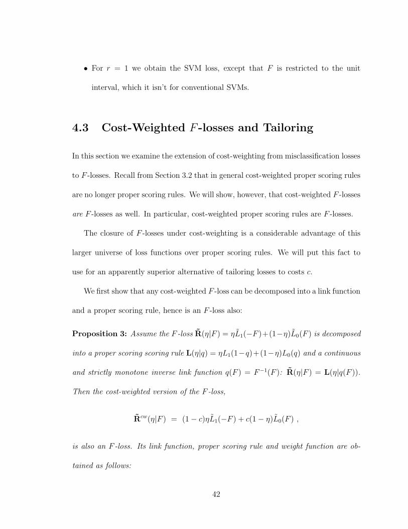
• For r = 1 we obtain the SVM loss, except that F is restricted to the unit
interval, which it isn’t for conventional SVMs.
4.3 Cost-Weighted F -losses and Tailoring
In this section we examine the extension of cost-weighting from misclassification losses
to F -losses. Recall from Section 3.2 that in general cost-weighted proper scoring rules
are no longer proper scoring rules. We will show, however, that cost-weighted F -losses
are F -losses as well. In particular, cost-weighted proper scoring rules are F -losses.
The closure of F -losses under cost-weighting is a considerable advantage of this
larger universe of loss functions over proper scoring rules. We will put this fact to
use for an apparently superior alternative of tailoring losses to costs c.
We first show that any cost-weighted F -loss can be decomposed into a link function
and a proper scoring rule, hence is an F -loss also:
Proposition 3: Assume the F -loss R(η|F ) = ηL1(−F )+(1−η)L0(F ) is decomposed
into a proper scoring scoring rule L(η|q) = ηL1(1−q)+(1−η)L0(q) and a continuous
and strictly monotone inverse link function q(F ) = F−1(F ): R(η|F ) = L(η|q(F )).
Then the cost-weighted version of the F -loss,
Rcw(η|F ) = (1− c)ηL1(−F ) + c(1− η)L0(F ) ,
is also an F -loss. Its link function, proper scoring rule and weight function are ob-
tained as follows:
42

1. The link function of the cost-weighted F -loss is
F cw(q) = F
(
(1− c)q
(1− c)q + c(1− q)
)
.
2. The proper scoring rule of the cost-weighted F -loss is given by
Lcw1 (1− q) = (1− c)L1
(
c(1− q)
(1− c)q + c(1− q)
)
,
Lcw0 (q) = cL0
(
(1− c)q
(1− c)q + c(1− q)
)
.
3. If the proper scoring rule is differentiable, the weight function for the cost-
weighted analog is
ωcw(q) = ω
(
(1− c)q
(1− c)q + c(1− q)
)
(1− c)2c2
((1− c)q + c(1− q))3.
The proof can be found in the appendix. If we write qcw(F ) = F cw−1(F ), and if we
further abbreviate qcw = qcw(F ) and q = q(F ), then the first assertion is equivalent
to
qcw
1− qcw=
c
1− c·
q
1− q
and
qcw =cq
cq + (1− c)(1− q).
It should be kept in mind that q(F ) does not provide consistent or calibrated prob-
ability estimates; qcw(F ) does. The role of equations relating the two is to indicate
the functional form that cost-weighted probability estimates qcw(F ) take. Because
q = 1/2 gets mapped to qcw = c, the class 1 decision regions q > 1/2 and qcw > c are
the same.
43

For tailoring to a specific cost c along the lines of Section 3.4, we need the first
and second moments of the normalized cost-weighted weight function ωcw(q). Recall
that the first moment is needed to match the weight function to the cost c, and the
second moment is needed as a measure of approximation to the point mass δc, which
is the “weight function” of cost-weighted misclassification loss.
Proposition 4: If ω(q) is a density function on (0, 1) with mean µ and variance σ2,
then
ωcw(q)
cµ + (1− c)(1− µ)
is also a density function, and its mean is
µcw =cµ
cµ + (1− c)(1− µ).
Its variance is bounded by
c(1− c) min(c, 1− c)
(cµ + (1− c)(1− µ))3σ2 ≤ σcw2 ≤
c(1− c) max(c, 1− c)
(cµ + (1− c)(1− µ))3σ2 .
The proof can be found in the appendix. Here is the application that provides the
basis for tailoring with cost-weighting:
Corollary: If ω(q) is a symmetric density with existing expectation, µ = 1/2, then
µcw = c
and
8 c (1− c) min(c, 1− c) σ2 ≤ σcw2 ≤ 8 c (1− c) max(c, 1− c) σ2 .
44

Thus cost-weighting a symmetric weight function with costs c and 1 − c readily
achieves tailoring for cost c.
It is somewhat dissatisfying that we are left with mere inequalities for the variance,
although they are sufficient for our purposes: if ω(q) becomes more spiky around 1/2
in terms of σ → 0, then ωcw(q) becomes more spiky around c in terms of σwc → 0
at the same rate. For a more complete result with an exact formula for σcw one has
to be more specific about ω(q). This works out for example if ω(q) is a symmetric
Beta weight function, but the formula is not a pretty sight. We start with a general
observation about symmetric Beta weights:
Corollary: If ω(q) ∼ qα−1(1 − q)α−1 is a symmetric Beta weight function, then the
cost-weighted version is
ωcw(q) ∼qa−1(1− q)a−1
((1− c)q + c(1− q))2α+1
It is merely this denominator that achieves the redistribution of the weight func-
tion so as to center it at µcw = c. An exact expression for the corresponding variance
is as follows:
Proposition 5: If ω(q) = qα−1(1− q)α−1/B(α, α) is a symmetric Beta density, then
the normalized cost-weighted density has the following variance:
σcw2 = c2
(
(α + 1)
(1− c)(2α + 1)2F1
(
1, α + 2, 2α + 2;1− 2c
1− c
)
− 1
)
.
45

where 2F1() is the hypergeometric function.
Again, the proof can be found in the appendix. It seems somewhat surprising that
mere cost-weighting causes such complications. There may not be much intuition
behind the above formulas, but the concept behind them, namely cost-weighting, is
simple enough, and the application to tailoring of weights is useful as we will show.
In the remainder of the section we discuss the shape of the cost-weighted weight
functions for the symmetric Beta family.
• For α > 1 the weight function has a mode at
−(α − 2(3c− 1)) +√
(α− 2(3c− 1))2 + 12c(2c− 1)(α− 1)
6(2c− 1)
In general, the mode and the expected value do not coincide. Thus if one wants
to put most of the weight on a certain threshold, one can set the above formula
to the desired value and backward calculate the corresponding cost c that is to
be applied to the cost-weighted F -loss.
• In the limit as α→∞, the weight function puts all mass at q = c. This follows
from the proposition that links α and σcw2.
• For α < 1, the weight function has a U-shape that puts more weight on the two
tails.
• For α = 1 and c 6= 1/2, depending on whether c is greater than 1/2 or not, the
weight function is either increasing or decreasing, thus puts more weight on one
tail.
46
0.0 0.2 0.4 0.6 0.8 1.0
0.00
0.05
0.10
0.15
0.20
0.25
0.30
q
L(q)
a= 16a= 11
a= 6
a= 2
a= Inf
0.0 0.2 0.4 0.6 0.8 1.0
01
23
45
q
omeg
a(q)
a= 16
a= 11
a= 6
a= 2
Figure 4.1: Loss functions L0(q) and weight functions ω(q) for various values of α,
and c = 0.3: Shown are α = 2, 6 ,11 and 16 scaled to show convergence to the step
function.
The calculations are given in the Appendix. Figure 4.1 illustrates the cost-weighted
weight functions and proper scoring rules for c = 0.3.
4.4 Margin-based Loss Functions
In this section we derive the connection between F -losses and margin-based loss func-
tions which have motivated many popular classification methods including boosting
and SVM. Yi Lin(2001) gave a nice discussion of margin-based loss functions where
he showed that many such loss functions are Fisher consistent in that they gener-
ate a classification procedure that is equivalent to Bayes’ rule for classification at the
47
c = 1/2 boundary. Here is a formal definition of margin-based losses: A margin-based
loss function is any loss function that can be written as
L(−Y ∗F )
where L(.) is a monotone increasing function and Y ∗ = 2Y−1 maps 0/1 coding of class
labels to ±1 coding. The quantity Y ∗F is called “the margin” and can be interpreted
as the “signed distance” of F from the boundary F = 0. Classification is done
according to Y ∗ = sign(F ) = 2 ∗ 1[F≥0]. A negative sign of Y ∗F is hence interpreted
as being on the wrong side of the boundary F = 0 indicating misclassification.
Expanding the above expression we get
L(−Y ∗F ) = L(−(2Y − 1)F ) = Y L(−F ) + (1− Y )L(F ) .
We recognize that such a loss is a special case of F -losses in which one sets both
L1 and L0 equal to L, assuming that additional conditions are satisfied that permit
the decomposition into a proper scoring rule and a link function. We can also see
that such a loss treats the two classes symmetrically, thus forcing equal costs on the
two types of misclassification error. Therefore, for the purpose of cost weighting, one
must allow asymmetry between the classes and use separate L1 and L0:
y ∗ L1(−F ) + (1− y) ∗ L0(F ) .
This in turn allows us to cost-weight the losses,
(1− c) ∗ y ∗ L1(−F ) + c ∗ (1− y) ∗ L0(F ) ,
which means replacing L1 with (1− c)L1 and L0 with c L0.
48
Chapter 5
IRLS for Linear Models
This chapter deals with optimization of F -losses for linear models. We start with
fitting a linear model for logistic regression by minimizing the negative log-likelihood
and show that the algorithm can be interpreted as an Iteratively Reweighted Least
Squares algorithm. Then we generalize the IRLS algorithm from logistic regression
to arbitrary proper scoring rules and F -losses, thus permitting us to play with the
choice of weights that induce loss functions.
5.1 IRLS for Proper Scoring Rules
Logistic regression is commonly computed with an Iteratively Reweighted Least Squares
or IRLS algorithm. We show that IRLS carries over to proper scoring rules in general.
Recall the form of a general proper scoring rule for a Bernoulli model:
L(η|q) = ηL1(1− q) + (1− η)L0(q)
49
A linear model is given by F (q) = xTb or, equivalently, q(F ) = q(xTb) using the
inverse link. We assume the data is an i.i.d. sample (xn, yn) (n = 1, ...,N) where xn
are drawn from a distribution in predictor space. For brevity we write
qn = q(F (xn)) , q′n = q′(F (xn)) , q′′n = q′′(F (xn)) .
We minimize the empirical risk, that is, the mean of a proper scoring rule over the
observations:
R(b) =1
N
∑
n=1,...,N
[ynL1(1− qn) + (1− yn)L0(qn)]
For concreteness we recall that this specializes for logistic regression to the well-known
form
R(b) = −1
N
∑
n=1,...,N
[yn log(qn) + (1− yn) log(1− qn)]
For a Newton update we need the gradient and the Hessian. First the gradient:
∂bR = −1
N
∑
n=1,...,N
(yn − qn)ω(qn)q′nxn,
For logistic regression, ω(q) = 1/(q(1 − q)) and q(F ) = 1/(1 + exp(−F )). A sim-
plification peculiar to logistic regression occurs because q′(F ) = q · (1 − q), hence
ω(q)q′(F ) = 1 and therefore
∂bR = −1
N
∑
n=1,...,N
(yn − qn)xn .
Setting the gradient to zero results in the so-called score equation.
The Hessian for the mean of the proper scoring rule is
∂2bR =
1
N
∑
n=1,...,N
[ω(qn)q′2n − (yn − qn)
(
ω′(qn)q′2n + ω(qn)q′′n)
]xnxTn . (5.1)
50
Specializing again to logistic regression, we observe that ω′ = −(1 − 2q)/(q(1− q))2
and q′′ = (1− 2q)q(1− q) and hence the second term of the Hessian disappears and
we obtain:
∂2bR = −
1
N
∑
n=1,...,N
qn(1− qn)xnxTn
A Newton step has the form
bnew = bold −(
∂2bR(b)
)−1(∂bR(b))
In direct generalization of IRLS for logistic regression, we can write the update as an
IRLS step for general proper scoring rules:
bnew = bold + (XT WX)−1XT z
where the ‘working weights’ and the ‘working responses’ are, respectively,
wn = ω(qn)q′2n − (yn − qn)(
ω′(qn)q′2n + ω′(qn)q′′n)
(5.2)
zn = (yn − qn)ω(qn)q′n/wn (5.3)
Denote by y the vector of responses y′ns, by X the N×(d+1) matrix with rows xT
n , by
q the vector of fitted probabilities with nth element qn, and by W a N × N diagonal
matrix with weights wn in the diagonal. The vectorized equation above shows that
the Newton updates can be written as solutions of a weighted least squares problem,
with iteration-dependent weights and responses. We wrote the IRLS update in an
incremental form whereas in the form usually shown in the literature one absorbs bold
in the working response z. We prefer the incremental form because of our interest in
stagewise fitting, which is an incremental procedure.
51
Specializing once again to logistic regression, we obtain the following familiar
expressions:
wn = qn (1− qn)
zn =(yn − qn)
qn (1− qn)
5.2 Fisher Scoring
For Fisher scoring one replaces the Hessian ∂2bR(b) with its expectation, assuming
the current estimates of the conditional probabilities of the labels to be the true ones:
P[Y = 1|X = xn] = qn. This means Eyn(yn − qn) = 0, hence the weights and the
working response simplify as follows:
wn = ω(qn) q′n2
, (5.4)
zn = (yn − qn)/q′n . (5.5)
Some observations:
• The function ω(q) is the contribution to the working weights wn due to the
proper scoring rule. Logistic regression with ω(q) = q−1(1 − q)−1 up-weights
extreme probabilities near zero and one.
• The term q′2 is the contribution to the working weights wn due to the link
function.
• The losses do not enter in the working response zn.
52
• The observed responses yn do not enter in the current weights wn.
It is well known that for logistic regression with log-loss and the logistic link, Fisher
scoring and Newton iterations coincide. From a machine learning perspective, it
is curious to learn that there exist loss functions for which the dependence of the
weights on the responses disappears for structural reasons: this is the case for so-
called “canonical links”, which are well-known in statistics from generalized linear
models. They have a generalization to certain combinations of proper scoring rules
and link functions as we will show now.
5.3 Canonical Links: Equality of Observed and
Expected Hessians
We examine under what condition on the combination of proper scoring rules and
link functions, Newton steps and Fisher scoring steps are identical. The requirement
is
R′′(b) = Ey [R′′(b) ] .
This condition is equivalent to requiring the weights wn in Equation (5.1) to be
independent of yn, which in turn is equivalent to
ω′(q) q′2
+ ω(q) q′′ = 0 .
53

This differential equation can be solved immediately: The left side equals ( ω(q) q′ )′,
hence ω(q) q′ is a constant, which we may choose to be 1:
ω(q) q′ = 1 .
Since q = q(F ) is the inverse of the link function F = F (q), we have F ′(q) =
1/q′(F (q)), and hence
F ′(q) = ω(q) = L′1(1− q) + L′
0(q) , (5.6)
where the second equality follows from L′1(1−q)+L′
0(q) = (1−q)ω(q)+ qω(q), which
is the sum of the Equations (3.1). The solution, unique up to an irrelevant additive
constant, is therefore
F (q) =
∫ q
ω(q)dq = L0(q)− L1(1− q) . (5.7)
We summarize:
Proposition 6: For any proper scoring rule there exists a canonical link function
F (q). The link function is unique up to a constant.
Here are the usual examples in the Beta family of proper scoring rules for α = β =
1, 0, -1/2 (Section 3.4):
• Squared error loss: L1(1− q) = (1− q)2 and L0(q) = q2, hence the inverse link
is
F (q) = 2q − 1 .
The canonical link is essentially the identity transform.
54

• Log-loss: L1(1− q) = − log(1− q) and L0(q) = − log(q), hence the natural link
is
F (q) = logq
1− q.
Its inverse is the logistic function.
• Boosting loss: L1(1− q) = ((1− q)/q)1/2 and L0(q) = (q/(1− q))1/2, hence the
natural link is
F (q) =
(
q
1− q
)1/2
−
(
1− q
q
)1/2
.
Its inverse is
q(F ) =1
2+
(
F
2
)
(
(
F
2
)2
+ 1
)−1/2
.
The F -loss is given by
L0/1(F ) =F
2+
(
(
F
2
)2
+ 1
)1/2
.
We see that the decomposition of the exponential loss into a proper scoring rule and
a link function does not result in a canonical pairing in which the observed and the
expected Hessian are idential. For exponential loss Newton iterations are not identical
with Fisher scoring iteration.
We conclude by noting that the converse of the above proposition holds also:
prescribing a link function as canonical essentially determines the proper scoring
rule.
Proposition 7: For any link function F (q) there exists a proper scoring rule for
which F (q) is canonical. The proper scoring rule is unique up to an additive constant.
55

This is immediately seen from Equation (5.6): F ′(q) = ω(q), and the fact that,
by Equations (3.1), ω(q) determines L1(1− q) and L0(q) up to a constant.
5.4 Newton Updates and IRLS for F -losses
For Newton updates based on general F -losses, the ingredients are
R(b) =1
N
∑
n=1..N
[
yn L1(−xTnb) + (1− yn) L0(yn xT
nb)]
,
∂bR(b) =1
N
∑
n=1..N
[
−yn L′1(−xT
nb) + (1− yn) L′0(x
Tnb)]
xn ,
∂2bR(b) =
1
N
∑
n=1..N
[
yn L′′1(−xT
nb) + (1− yn) L′′0(x
Tnb)]
xnxTn .
The current IRLS weights and responses are therefore
wn = yn L′′1(−xT
nb) + (1− yn) L′′0(x
Tnb) ,
zn = ynL′
1(−xTnb)
L′′1(−xT
nb)− (1− yn)
L′0(x
Tnb)
L′′0(x
Tnb)
.
Specializing to symmetric F -losses with L = L1 = L0, the ingredients of Newton
updates are
R(b) =1
N
∑
n=1..N
L(−y∗n xT
nb) ,
∂bR(b) =1
N
∑
n=1..N
L′(−y∗n xT
nb) (−y∗n)xn ,
∂2bR(b) =
1
N
∑
n=1..N
L′′(−y∗n xT
nb)xnxTn ,
where we made use of (y∗n)2 = 1. A Newton increment − (∂2
bR(b))
−1(∂bR(b)) can be
56
written as a weighted LS solution with the following current weights and responses:
wn = L′′(−y∗n xT
nb) ,
zn =L′(−y∗
n xTnb)
L′′(−y∗n xT
nb)y∗
n .
For exponential loss L(F ) = exp(F ), some simplifications occur:
wn = exp(−y∗n xT
nb) , zn = y∗n .
The weights are exactly those of the boosting algorithm in the next section with
Fn = xTnb.
These algorithms are worthwhile keeping in mind for the common cases where the
losses Li and hence R(b) are convex, as is the case for exponential loss. Convexity
and the ensuing stability of minimization may get obscured when an F -loss is decom-
posed into a link function and a proper scoring rule. On the other hand, in those
cases where the weight function ω(q) is tailored for classification with unequal cost
of misclassification, the F -loss is unlikely to be convex, and stability may be gained
by using Fisher scoring instead, whose expected Hessian is always positive definite.
5.5 Convexity of F -losses
Convexity of F -losses is of interest for two reasons:
• When the F -loss is convex, Newton steps may be more efficient than Fisher
scoring steps.
57

• Convexity of F -losses is assumed in theoretical work on consistency of classifica-
tion schemes, as for example in Lugosi and and Vayatis (2004) and Zhang (2004).
A special case of convex F -loss arises when a proper scoring rule is matched with
its canonical link function. Convexity follows because for canonical links the empirical
Hessian and the expected Hessian coincide, and the expected Hessian is always non-
negative definite. Convexity is more general than the case of canonical links, though.
For example, we saw above that the link function of exponential loss is not canonical,
that is, observed and expected Hessians do not coincide, yet exponential loss as a
F -loss is convex.
We give a general condition under which a pairing of a link function and a proper
scoring rule results in a convex F -loss. The condition is derived by requiring the
weights in the Hessian of Equation (5.2) to be non-negative: wn ≥ 0, that is,
ω(q) q′2− (y − q)
(
ω′(q) q′2
+ ω(q) q′′)
≥ 0 .
This requirement results in two redundant inequalities, one for y = 1 and one for
y = 0. We summarize:
Proposition 8: A combination of proper scoring rule and link function results in a
convex loss R(b) if ω(q) and q(F ) satisfy
−1
q≤
ω′
ω+
q′′
q′2≤
1
1− q.
58

As a corollary, the combination of proper scoring rules in the Beta family with
equal exponents,
ω(q) = qα−1(1− q)β−1 ,
and scaled logistic links,
q(F ) = 1/(1 + e−F/s) , F (q) = s logq
1− q,
result in convex F -losses iff
−1 ≤ α, β ≤ 0 , s > 0 .
These proper scoring rules result in convex F -losses for any scaled logistic link. Special
cases are exponential loss (α = β = −1/2, s = 1/2) and log-loss with the logit scale
(α = β = 0, s = 1). But squared error loss (α = β = 1) does not result in convex
F -losses with any scaled logistic link.
For the combination of the cost-weighted Beta family,
ωcw(q) ∼qa−1(1− q)a−1
((1− c)q + c(1− q))2α+1,
and the cost-weighted logistic link,
qcw(F ) =c
c + (1− c)e−F/s, F cw(q) = s log
q
1− q− s log
c
1− c, (5.8)
convexity of the resulting cost-weighted F -losses holds iff
−1 ≤ α ≤ 0 , s > 0 .
This includes exponential loss for α = −1/2 and s = 1/2 as well as logistic loss for
α = 0 and s = 1.
59

5.6 Some Peculiarities of Exponential Loss
Exponential loss has some special properties under cost-weighting. We see that for
α = β = −1/2 the denominator of the cost-weighted weight function is constant and
hence:
ωcw(q) ∼ q−3/2(1− q)−3/2 .
That is, the weight function does not depend on the cost c. The link function, however,
depends on c according to Equation (5.8). In effect, cost-weighting exponential loss
is achieved by shifting the modeling scale alone:
F (q) = s logq
1− q− s log
c
1− c
Because for cost-weighted link functions one still has q′(F ) = q(1− q)/s, the working
weights look superficially the same as without cost-weighting: wn = 1/s2 · [q(1−q)]1/2.
However, the meaning of q = q(F ) has changed because this is now the shifted logistic
link.
60
Chapter 6
Stagewise Fitting of Additive
Models
6.1 Boosting
Boosting is an algorithm that has achieved huge success in the field of machine learn-
ing. It combines a group of weak classifiers a weighted voting scheme so that a strong
learner results. In the following we describe the most common version of the boosting
algorithm, discrete Adaboost, which was proposed by Freund and Schapire (1996):
Suppose the response y∗n is labeled as -1 or 1,
1. Start with weights wn = 1/N , n = 1, ..., N .
2. For m = 1 to M :
(a) Fit a classifier fm(x) to the training data using weights wn.
61

(b) Compute the weighted misclassification error of fm(x):
errm =
∑
n=1,...,N wnI(y∗n 6= fm(xn))
∑
n=1,...,N wn
(c) Compute the logit of the weighted misclassification error:
αm = log
(
1− errm
errm
)
(d) Set wn ← wn · exp[αm · I(y∗n 6= fm(xn))], n = 1, ...,N.
3. Output sign[∑
m=1,...,M αmfm(x)] as the ±1-labeled classifier.
Adaboost up-weights those points that are misclassified according to how well the
classifier performs at the current iteration. Thus intuitively, the classifier would focus
more on the hard cases in the next round.
In FHT(2000), Adaboost was viewed as stagewise additive fitting which exploits
Newton steps to optimize exponential loss, which we write as follows with non-
parametric fits in mind:
R =1
N
∑
n=1...N
L(−y∗n Fn) , L(F ) = exp(F ) .
The Newton updates are based on the following components:
wn = exp(−ynF oldn ) , zn = yn ,
where F has the additive form
F (x) =∑
t=1,...,T
ft(x)
In their paper, FHT also created LogitBoost which optimizes log-loss by fitting a
stagewise additive model.
62
6.2 Stagewise Fitting of Additive Models by Op-
timizing General Losses
In this section we adopt FHT’s view of boosting and adapt the IRLS iterations to
stagewise forward additive modeling.
For additive modeling one needs a set F of possible basis functions f(x). An
additive model is a linear combination of elements of F : F (x) =∑
k bkfk(x). One
does not assume that F is a linear space because in a typical application of boosting
F would be a set of trees with a certain structure, such as stumps (trees of depth
one), that are not closed under linear combinations.
Stagewise fitting is the successive acquisition of terms f (K) ∈ F given that terms
f (1), . . . , f (K−1) for a model F (K−1) =∑
k=1..K−1 bk f (k) have already been acquired.
In what follows we write F old for F (K−1), f for f (K), b for bK , and finally Fnew =
F old + b f . For a loss function
R(F ) = Ex,y L(y|q(F (x))) ,
the conceptual goal is to find
(f, b) = argminf∈F , b∈IR R( F old + b f) .
Given a training sample {(xn, yn)}n=1..N , the loss is estimated by
R(F old + b f) =1
N
∑
n=1..N
L(yn | q( F old(xn) + b f(xn) )) .
With these modifications stagewise fitting can proceed according to the IRLS scheme
in such a way that each IRLS step produces a new term f , a coefficient b, and an
63
update F new = F old + b f based on current weights wn, current estimated class 1
probabilities qn, and current responses zn, as follows:
Fn = F old(xn) ,
qn = q(Fn) , q′n = q′(Fn) , q′′n = q′′(Fn) ,
wn = ω(qn) q′n2− (yn − qn)
(
ω′(qn) q′n2
+ ω(qn) q′′n
)
,
zn = (yn − qn) ω(qn) q′n/wn .
In practice, f is the result of some heuristic search procedure such as greedy tree
construction or, in the simplest case, search for the best fitting stump (a tree with
only one split). Whatever this may be, we denote it by
f ← feature-proposer(X, W, z) .
We can think of f as a proposal for a derived predictor vector f = (f(x1), ..., f(xN))T
which is to be used instead of X in the IRLS step at the current stage. The remaining
task is to optimize the coefficient b for f . Sometimes, the coefficient b is absorbed in
f because the feature-proposer may find b at the same time as it performs the search,
so no optimization is necessary. At other times, the coefficient b has to be optimized
explicitly, for example through a line search:
b = argminb
1
N
∑
n=1..N
L( yn | q(Fn + bfn) ) ,
or approximately by a simple weighted LS regression of z on f :
b =zT W f
fT W f.
64

The two standard examples for feature-proposers are the following:
• In “real Adaboost”, the class F is the set of trees of a fixed depth, which is
often only depth one and called “stumps”.
• In “discrete Adaboost”, the class F is the set of indicator functions of decision
regions obtained by thresholding trees.
Discrete Adaboost follows then the same heuristic tree construction as in real Ad-
aboost, followed by thresholding. When F is the set of stumps, the search for an
optimal stump can be performed exhaustively. In this case real and discrete Ad-
aboost are almost identical, except for the treatment of the intercept: real Adaboost
can adjust the intercept at each step due to the fitting of two constants (one on either
side of the split), whereas discrete Adaboost can fit only one constant, on the area
where the indicator is 1.
In general the role of the feature-proposer is to propose descent directions from
a stock of possible choices, the set F . The behavior of the feature-proposer and the
nature of the set F are of course crucial for the performance of the boosting scheme
based on them.
65

Chapter 7
Experiments
7.1 Examples of Biased Linear Fits with Successful
Classification
We illustrate the fact that linear models can be unsuitable as global models and yet
successful for classification at specific thresholds or, equivalently, for cost-weighted
misclassification loss. To this end we recreate an artificial example of Hand and
Vinciotti (2003) and show that our methods for tailoring loss functions to specific
classification thresholds allow us to estimate boundaries. We then show that the
Hand and Vinciotti (2003) scenario is a fair approximation to some well-known real
data, the Pima Indian diabetes data (UCI Machine Learning database). Finally we
apply our model to two more real data: German credit data and adult income data
from the UCI Machine learning database.
66
Example 1. Artificial data: We start with a linear model, that is, a composi-
tion q(bT x) of a linear function, bT x, and a link function, q(), as in logistic regression.
Note that the level curves, {x | q(bTx) = c }, are parallel lines. This fact can be used
to construct scenarios η(x) for which the model q(bTx) is globally inadequate and
yet can produce excellent classification boundaries. Such a construction was demon-
strated by Hand and Vinciotti (2003): they designed η(x) as a “rule surface” with
the shape of a smooth spiral ramp on the unit square, as depicted in Figure 7.1. The
critical feature of the surface is that the optimal classification boundaries η(x) = c
are all linear but not parallel. The absence of parallelism renders any linear model
q(bTx) unsuitable as a global fit, but the linearity of the classification boundaries al-
lows linear models to describe these boundaries, albeit every level requires a different
linear model. The point of Hand and Vinciotti’s (2003) and our schemes is to home
in on these level-specific models.
In recreating Hand and Vinciotti’s (2003) example, we simulated 4,000 data points
whose two predictors were uniformly distributed in the unit square, and whose class
labels had a conditional class 1 probability η(x1, x2) = x2/(x1+x2). We fitted a linear
model with the logistic link function q(t) = 1/(1+exp(t)), using a proper scoring rule
in the Beta family with α = 6 and α/β = 0.3/0.7 in order to home in on the c = 0.3
boundary (Section 3.4). We also fitted a linear model with the cost-weighted logistic
link q(t) = c/(c + (1 − c) exp(t)), where c = .3, using a proper scoring rule in the
cost-weighted Beta family with α = β = 4 (Section 4.3). Figure 7.1, which is similar
to Hand and Vinciotti’s (2003) Figure 1 shows the success: the estimated boundary is
67

close to the true 0.3-boundary. The figure also shows that the 0.3-boundary estimated
with the log-loss of logistic regression is essentially parallel to the 0.5-boundary, which
is sensible because logistic regression is bound to find a compromise model which, for
reasons of symmetry between the two labels, should be a linear model with level lines
roughly parallel to the true 0.5-boundary.
We also created a model which was based on a variation of Hand and Vinciotti’s
(2003) example. We simulated 4,000 data points whose two predictors were uniformly
distributed in the unit square, and whose class labels had a conditional class 1 prob-
ability η(x1, x2) = kx2/(x1 + kx2), where k is constant. The parameter k was used to
adjust the priors of the two classes, when k > 1, there were more class 1 than class 0,
otherwise there were more class 0 than class 1. In our simulated data, we set k = 5,
so class 1 was roughly 78% of the data. We would like to show that under an unbal-
anced design such as this, even when estimating a boundary η(x) = 0.5, one might
want to use a tailored loss other than log-loss. This is illustrated in Figure 7.2 which
shows the 0.3-boundary, 0.5-boundary and 0.7-boundary estimated with log-loss and
tailored losses. Indeed, the imbalance of the classes makes the tailored solutions
superior to log-loss even for the 0.5-boundary.
68
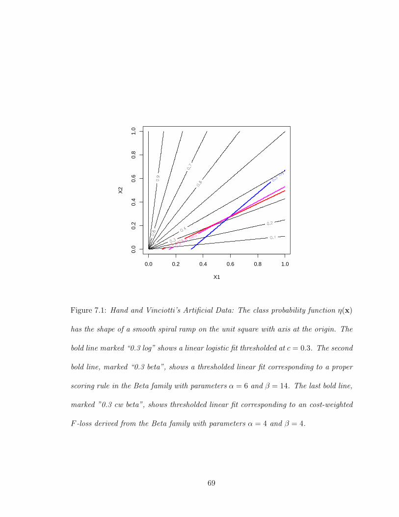
X1
X2
0.0 0.2 0.4 0.6 0.8 1.0
0.0
0.2
0.4
0.6
0.8
1.0
Figure 7.1: Hand and Vinciotti’s Artificial Data: The class probability function η(x)
has the shape of a smooth spiral ramp on the unit square with axis at the origin. The
bold line marked “0.3 log” shows a linear logistic fit thresholded at c = 0.3. The second
bold line, marked “0.3 beta”, shows a thresholded linear fit corresponding to a proper
scoring rule in the Beta family with parameters α = 6 and β = 14. The last bold line,
marked ”0.3 cw beta”, shows thresholded linear fit corresponding to an cost-weighted
F -loss derived from the Beta family with parameters α = 4 and β = 4.
69
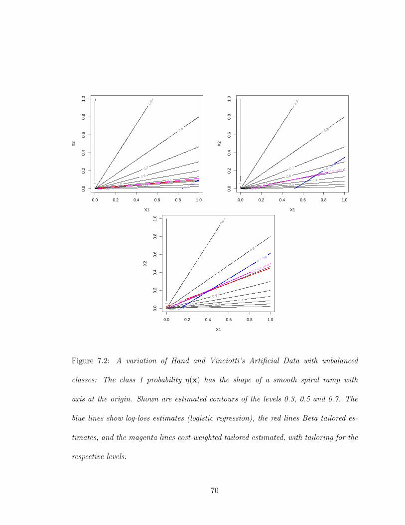
X1
X2
0.0 0.2 0.4 0.6 0.8 1.0
0.0
0.2
0.4
0.6
0.8
1.0
X1
X2
0.0 0.2 0.4 0.6 0.8 1.0
0.0
0.2
0.4
0.6
0.8
1.0
X1
X2
0.0 0.2 0.4 0.6 0.8 1.0
0.0
0.2
0.4
0.6
0.8
1.0
Figure 7.2: A variation of Hand and Vinciotti’s Artificial Data with unbalanced
classes: The class 1 probability η(x) has the shape of a smooth spiral ramp with
axis at the origin. Shown are estimated contours of the levels 0.3, 0.5 and 0.7. The
blue lines show log-loss estimates (logistic regression), the red lines Beta tailored es-
timates, and the magenta lines cost-weighted tailored estimated, with tailoring for the
respective levels.
70

Example 2. Pima data: Our first real data example shows that Hand and
Vinciotti’s stylized scenario is met in the well-known Pima Indians diabetes data
when restricting attention to the two major predictors, here labeled “PLASMA” and
“BODY”. Figure 7.3 shows scatterplots of these two predictors with glyph-coding of
the classes. We illustrate the estimation for c = .1, c = .5 and c = .8. Cost-weighted
tailoring seems to indicate the spiral shape the best.
But is there really a spiral ramp? We give independent evidence in Figure 7.4
which shows thresholded class probabilities that are estimated with a completely
different method, namely, the nearest-neighbor method. The figure clearly shows the
sweeping motion of the level curves as the level is raised, lending credence to the idea
that the level curves may be well-approximated by a set of non-parallel lines.
For comparison, we report in Tables 7.1, 7.2 and 7.3 the mean of 10-fold cross-
validated cost-weighted misclassification loss (error) for different costs c. The tailored
losses often yield slightly better and never worse results than log-loss. If the numbers
are to be believed, cost-weighted Beta tailoring may hold a slight edge over plain Beta
tailoring.
71
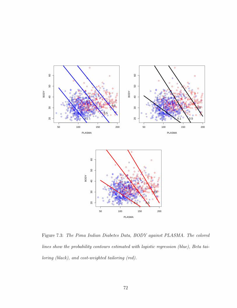
50 100 150 200
2030
4050
60
PLASMA
BO
DY
0.5
0.1
0.8
50 100 150 200
2030
4050
60PLASMA
BO
DY
0.50.1
0.8
50 100 150 200
2030
4050
60
PLASMA
BO
DY
0.50.1
0.8
Figure 7.3: The Pima Indian Diabetes Data, BODY against PLASMA. The colored
lines show the probability contours estimated with logistic regression (blue), Beta tai-
loring (black), and cost-weighted tailoring (red).
72
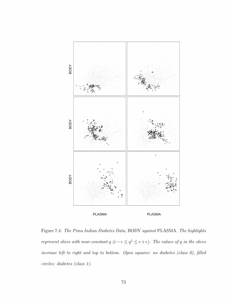
BO
DY
BO
DY
BO
DY
PLASMA PLASMA
Figure 7.4: The Pima Indian Diabetes Data, BODY against PLASMA. The highlights
represent slices with near-constant q (c− ǫ ≤ q1 ≤ c+ ǫ). The values of q in the slices
increase left to right and top to bottom. Open squares: no diabetes (class 0), filled
circles: diabetes (class 1).
73

Table 7.1: Pima Indian Diabetes: c = 0.1
class 1 error class 0 error cost-weighted error parameters
log-loss 0.5 36.7 0.055± 0.003 α = β = 0
Beta 0.7 34.4 0.054± 0.003 σopt = 0.08
cost-weighted 0.7 32.7 0.052± 0.004 αopt = 2
Table 7.2: Pima Indian Diabetes: c = 0.5
class 1 error class 0 error cost-weighted error parameters
log-loss 12.2 5.8 0.120± 0.008 α = β = 0
Beta 11.8 5.8 0.117± 0.009 αopt = 2
cost-weighted 11.8 5.8 0.117± 0.009 αopt = 2
Example 3. German credit data: This dataset has 1000 observations and 20
attributes of creditors of a bank. The goal is to predict the likelihood of good credit of
a customer. The data comes with a cost matrix that assigns a cost of 5 if a customer
is misclassified as good credit when he has actually bad credit, and a cost of 1 if a
customer is misclassified as bad credit when he actually has good credit. We labeled
a good credit as class 1 and a bad credit as class 0. Thus, to minimize the cost of
misclassification, we classify a customer as class 1 if η(x) > 1/6, otherwise class 0.
We compared again log-loss with Beta tailoring and cost-weighted tailoring. The
target threshold is c = 1/6 based on the given cost information. When evaluating the
models, we estimated α by fitting models on randomly selected 640 cases, optimiz-
74

Table 7.3: Pima Indian Diabetes: c = 0.8
class 1 error class 0 error cost-weighted error parameters
log-loss 20.7 1.4 0.070± 0.006 α = β = 0
Beta 21.6 1.3 0.072± 0.006 σopt = 0.18
cost-weighted 21.6 1.2 0.070± 0.006 αopt = 2
ing cost-weighted misclassification loss on 160 cross-validation cases, and measuring
performance on 200 hold-out cases, —repeating this whole procedure 100 times (=
20 times 5-fold holdouts). Thus each method is now characterized by 100 values of
honestly estimated cost-weighted misclassification errors.
We now compare these three sets of values with a graphical version of a 2-sample
permutation test. The upper panel of Figure 7.5 shows the result of the comparison
of log-loss and Beta-tailored loss: The blue line represents the empirical quantile-
quantile curve with the sorted Beta loss values on the horizontal axis and the sorted
log-loss values on the vertical axis. The red band is a spaghetti graph that overplots
many (100) empirical quantil-quantile curves when the labels “log-loss” and “Beta
loss” are randomly permuted against the (200) values of the estimated misclassifi-
cation losses. The fact that the blue curve stays within the red band shows that
the distributions of the log-loss and the Beta loss error values are indistinguishable
modulo randomness.
Similarly, the lower panel of Figure 7.5 shows the comparison of log-loss with
cost-weighted F -loss. In this case the blue curve is consistently above the red band,
75
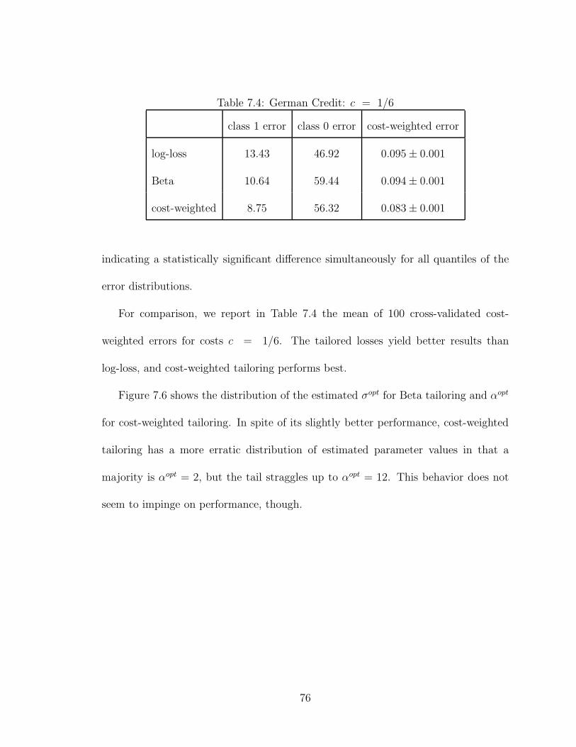
Table 7.4: German Credit: c = 1/6
class 1 error class 0 error cost-weighted error
log-loss 13.43 46.92 0.095± 0.001
Beta 10.64 59.44 0.094± 0.001
cost-weighted 8.75 56.32 0.083± 0.001
indicating a statistically significant difference simultaneously for all quantiles of the
error distributions.
For comparison, we report in Table 7.4 the mean of 100 cross-validated cost-
weighted errors for costs c = 1/6. The tailored losses yield better results than
log-loss, and cost-weighted tailoring performs best.
Figure 7.6 shows the distribution of the estimated σopt for Beta tailoring and αopt
for cost-weighted tailoring. In spite of its slightly better performance, cost-weighted
tailoring has a more erratic distribution of estimated parameter values in that a
majority is αopt = 2, but the tail straggles up to αopt = 12. This behavior does not
seem to impinge on performance, though.
76
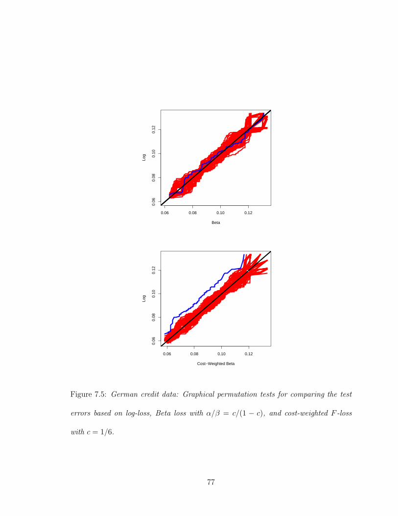
0.06 0.08 0.10 0.12
0.06
0.08
0.10
0.12
Beta
Log
0.06 0.08 0.10 0.12
0.06
0.08
0.10
0.12
Cost−Weighted Beta
Log
Figure 7.5: German credit data: Graphical permutation tests for comparing the test
errors based on log-loss, Beta loss with α/β = c/(1 − c), and cost-weighted F -loss
with c = 1/6.
77

0.08 0.1 0.12 0.14 0.16 0.18 0.2
sigma.opt
05
1015
20
0.1393 0.1144 0.0922 0.0887 0.0809 0.0700 0.0625 0.0570
sigma.opt(CW Beta)
05
1015
2025
30
Figure 7.6: Histogram of the estimated σ for Beta tailoring (upper panel)
and estimated α for cost-weighted tailoring (lower panel) for the German credit
data with c = 1/6. In the estimation of σ and α with optimization of
cross-validated cost-weighted error we constrained σ between 0.06 and 0.2 in
0.02 increments and α to {2, 3, 4, 5, 6, 8, 10, 12} with the corresponding σ to
{0.139,0.114,0.092,0.0887,0.081,0.070,0.063,0.057}.
78
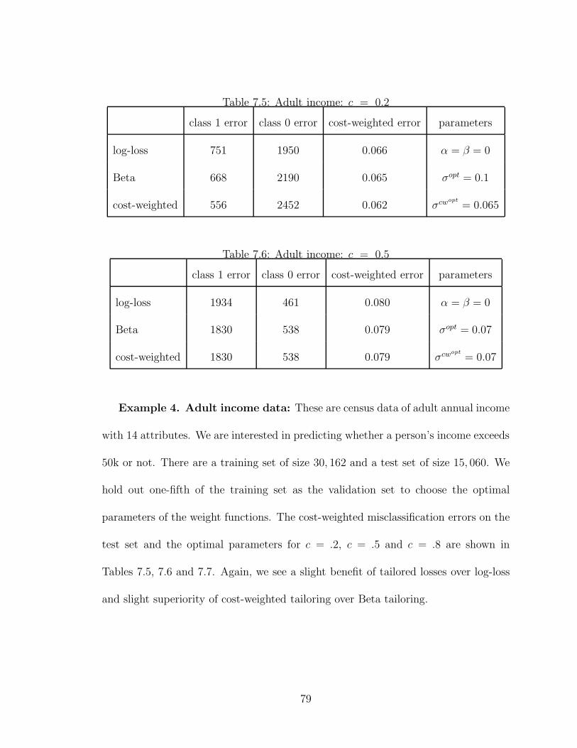
Table 7.5: Adult income: c = 0.2
class 1 error class 0 error cost-weighted error parameters
log-loss 751 1950 0.066 α = β = 0
Beta 668 2190 0.065 σopt = 0.1
cost-weighted 556 2452 0.062 σcwopt
= 0.065
Table 7.6: Adult income: c = 0.5
class 1 error class 0 error cost-weighted error parameters
log-loss 1934 461 0.080 α = β = 0
Beta 1830 538 0.079 σopt = 0.07
cost-weighted 1830 538 0.079 σcwopt
= 0.07
Example 4. Adult income data: These are census data of adult annual income
with 14 attributes. We are interested in predicting whether a person’s income exceeds
50k or not. There are a training set of size 30, 162 and a test set of size 15, 060. We
hold out one-fifth of the training set as the validation set to choose the optimal
parameters of the weight functions. The cost-weighted misclassification errors on the
test set and the optimal parameters for c = .2, c = .5 and c = .8 are shown in
Tables 7.5, 7.6 and 7.7. Again, we see a slight benefit of tailored losses over log-loss
and slight superiority of cost-weighted tailoring over Beta tailoring.
79
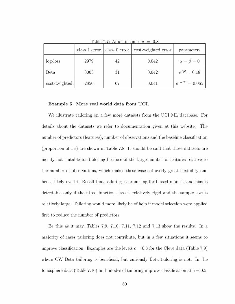
Table 7.7: Adult income: c = 0.8
class 1 error class 0 error cost-weighted error parameters
log-loss 2979 42 0.042 α = β = 0
Beta 3003 31 0.042 σopt = 0.18
cost-weighted 2850 67 0.041 σcwopt
= 0.065
Example 5. More real world data from UCI.
We illustrate tailoring on a few more datasets from the UCI ML database. For
details about the datasets we refer to documentation given at this website. The
number of predictors (features), number of observations and the baseline classification
(proportion of 1’s) are shown in Table 7.8. It should be said that these datasets are
mostly not suitable for tailoring because of the large number of features relative to
the number of observations, which makes these cases of overly great flexibility and
hence likely overfit. Recall that tailoring is promising for biased models, and bias is
detectable only if the fitted function class is relatively rigid and the sample size is
relatively large. Tailoring would more likely be of help if model selection were applied
first to reduce the number of predictors.
Be this as it may, Tables 7.9, 7.10, 7.11, 7.12 and 7.13 show the results. In a
majority of cases tailoring does not contribute, but in a few situations it seems to
improve classification. Examples are the levels c = 0.8 for the Cleve data (Table 7.9)
where CW Beta tailoring is beneficial, but curiously Beta tailoring is not. In the
Ionosphere data (Table 7.10) both modes of tailoring improve classification at c = 0.5,
80

Table 7.8: Description of More UCI Data
cleve ionosphere spect wdbc wpbc
number of features 13 34 22 30 33
number of observations 296 351 267 569 194
proportions of 1’s 54% 64% 79% 37% 24%
Table 7.9: CW-Error for Data Cleve
c = 0.2 c = 0.5 c = 0.8
log-loss 0.055± 0.009 0.086± 0.011 0.065± 0.007
Beta 0.064± 0.010 0.082± 0.010 0.071± 0.008
cost-weighted 0.062± 0.011 0.082± 0.010 0.057± 0.007
but neither at c = 0.2 nor c = 0.8. For the next two datasets, Spect and Wdbc
(Tables 7.11 and 7.12), no benefit is discernable. The last dataset, Wpbc (Table 7.13)
shows an improvement for c = 0.5 but not for c = 0.2 and c = 0.8.
If there is a message, it is that the benefits of tailoring cannot be predicted without
trying. Essentially, one has to try a range of values α as we did in these data examples
where α was selected with cross-validation. [In detail: We form a training set of size
80%; we partition the training set again into a subset of 80% and and a hold-out set
of 20% to determine α; then we apply the model with the estimated α to the whole
training set and evaluate out-of-sample misclassication on the test set.]
81
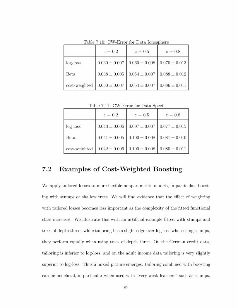
Table 7.10: CW-Error for Data Ionosphere
c = 0.2 c = 0.5 c = 0.8
log-loss 0.030± 0.007 0.060± 0.008 0.070± 0.013
Beta 0.038± 0.005 0.054± 0.007 0.088± 0.012
cost-weighted 0.030± 0.007 0.054± 0.007 0.086± 0.011
Table 7.11: CW-Error for Data Spect
c = 0.2 c = 0.5 c = 0.8
log-loss 0.043± 0.006 0.097± 0.007 0.077± 0.015
Beta 0.041± 0.005 0.100± 0.008 0.081± 0.010
cost-weighted 0.042± 0.006 0.100± 0.008 0.080± 0.011
7.2 Examples of Cost-Weighted Boosting
We apply tailored losses to more flexible nonparametric models, in particular, boost-
ing with stumps or shallow trees. We will find evidence that the effect of weighting
with tailored losses becomes less important as the complexity of the fitted functional
class increases. We illustrate this with an artificial example fitted with stumps and
trees of depth three: while tailoring has a slight edge over log-loss when using stumps,
they perform equally when using trees of depth three. On the German credit data,
tailoring is inferior to log-loss, and on the adult income data tailoring is very slightly
superior to log-loss. Thus a mixed picture emerges: tailoring combined with boosting
can be beneficial, in particular when used with “very weak learners” such as stumps,
82
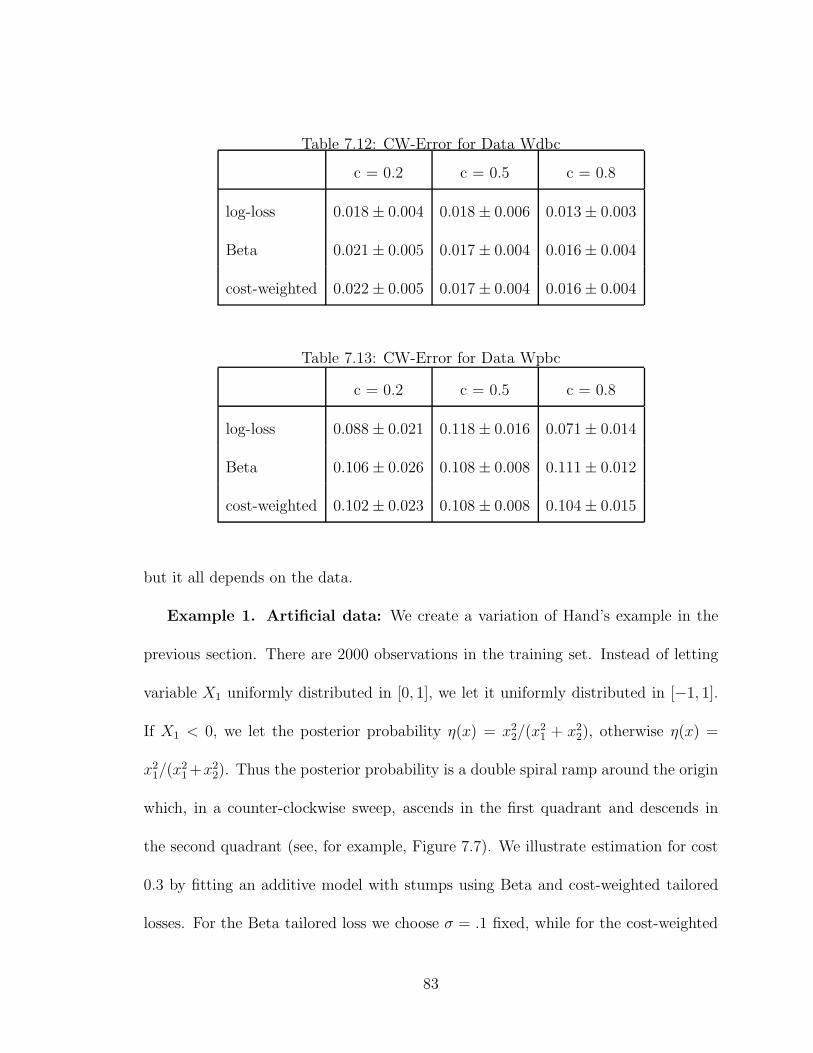
Table 7.12: CW-Error for Data Wdbc
c = 0.2 c = 0.5 c = 0.8
log-loss 0.018± 0.004 0.018± 0.006 0.013± 0.003
Beta 0.021± 0.005 0.017± 0.004 0.016± 0.004
cost-weighted 0.022± 0.005 0.017± 0.004 0.016± 0.004
Table 7.13: CW-Error for Data Wpbc
c = 0.2 c = 0.5 c = 0.8
log-loss 0.088± 0.021 0.118± 0.016 0.071± 0.014
Beta 0.106± 0.026 0.108± 0.008 0.111± 0.012
cost-weighted 0.102± 0.023 0.108± 0.008 0.104± 0.015
but it all depends on the data.
Example 1. Artificial data: We create a variation of Hand’s example in the
previous section. There are 2000 observations in the training set. Instead of letting
variable X1 uniformly distributed in [0, 1], we let it uniformly distributed in [−1, 1].
If X1 < 0, we let the posterior probability η(x) = x22/(x2
1 + x22), otherwise η(x) =
x21/(x2
1 +x22). Thus the posterior probability is a double spiral ramp around the origin
which, in a counter-clockwise sweep, ascends in the first quadrant and descends in
the second quadrant (see, for example, Figure 7.7). We illustrate estimation for cost
0.3 by fitting an additive model with stumps using Beta and cost-weighted tailored
losses. For the Beta tailored loss we choose σ = .1 fixed, while for the cost-weighted
83
tailored loss we choose α = 4 (σ = 0.10)fixed. (In particular, we do not estimate
these parameters from the data.) We then compare the results tailoring with log-loss,
which is FHT’s (2000) LogitBoost.
Figure 7.7 shows contour plots for the estimation of the .3 boundary when using
log-loss, tailored Beta loss and cost-weighted tailored loss at iteration 50. None of the
models generates accurate estimation in terms of geometrically correct boundaries.
Clearly log-loss performs the poorest. Yet, by using the tailored loss, one can recover
one side of the boundary. After 50 iterations, the stumps start to overfit. From
Figure 7.8, one can see that at iteration 300 stumps fit many small windows on one
side of the boundary yet they are never able to better approximate the boundary on
the other side. Log-loss shows a more symmetric attempt at capturing both sides of
the boundary.
Figure 7.9 shows the average cost-weighted misclassification losses for 10 simula-
tions on a test set of size 10, 000. In this artificial example, tailoring wins over log-loss
by a considerable margin of about 2%! We also notice a mild tendency to overfit after
about 50 iterations, an indication that boosting is in fact not immune to overfitting,
as is now common knowledge.
However, if we fit trees with depth three to this data, the advantage of tailoring
disappears. Figure 7.10 shows the estimate of the probability contour for c = .3 at
iteration 10. There is no significant difference between the tailored loss and log-loss.
Figure 7.11 shows the cost-weighted test error of log-loss and tailored losses. If one is
willing to fit a more complex model in this case, then it is overfitting that one should
84

worry about instead of the tailoring.
85
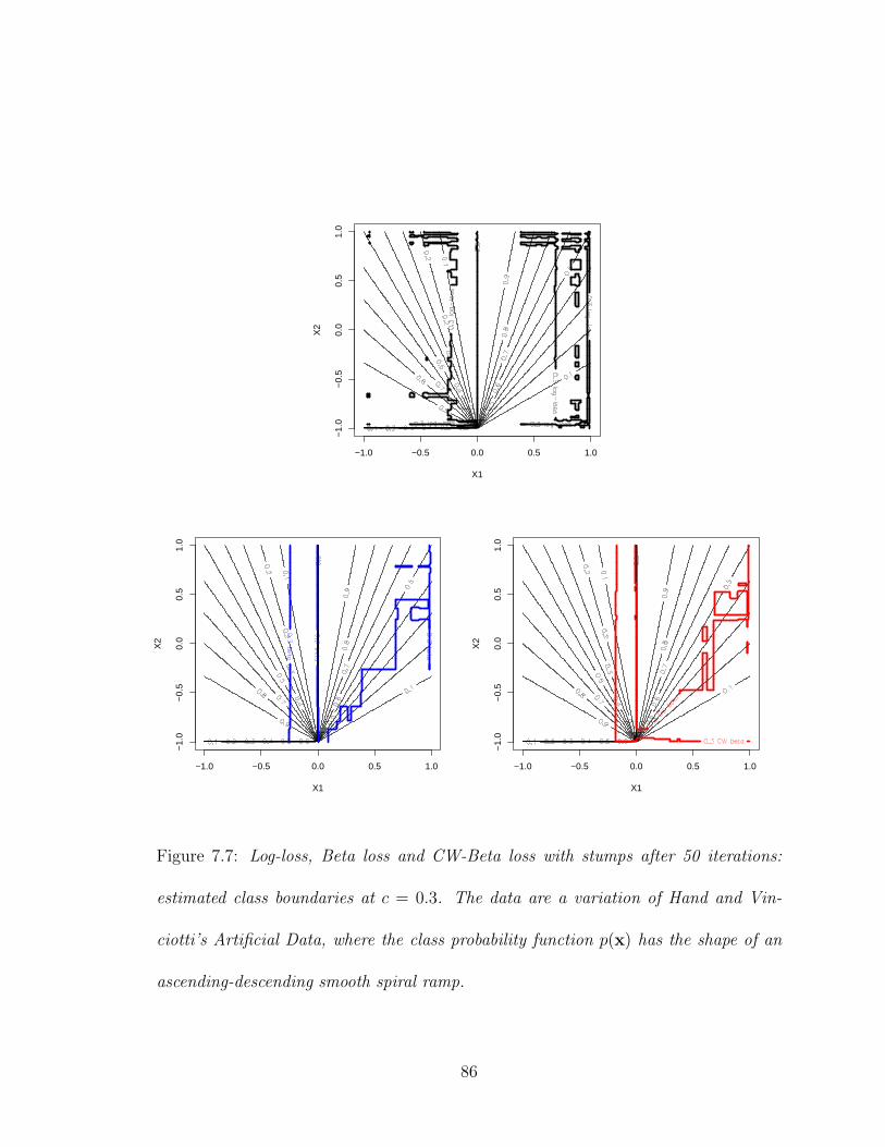
X1
X2
−1.0 −0.5 0.0 0.5 1.0
−1.
0−
0.5
0.0
0.5
1.0
X1
X2
−1.0 −0.5 0.0 0.5 1.0
−1.
0−
0.5
0.0
0.5
1.0
X1
X2
−1.0 −0.5 0.0 0.5 1.0
−1.
0−
0.5
0.0
0.5
1.0
Figure 7.7: Log-loss, Beta loss and CW-Beta loss with stumps after 50 iterations:
estimated class boundaries at c = 0.3. The data are a variation of Hand and Vin-
ciotti’s Artificial Data, where the class probability function p(x) has the shape of an
ascending-descending smooth spiral ramp.
86
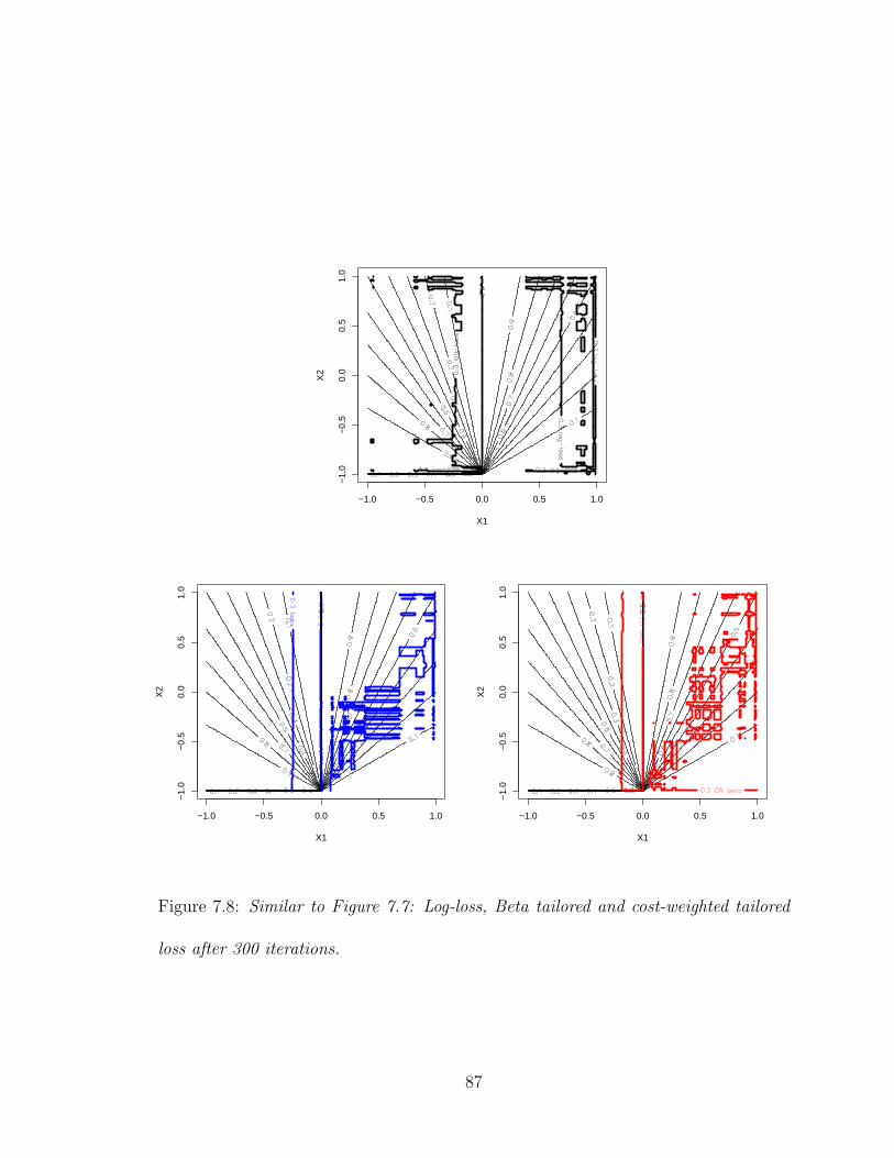
X1
X2
−1.0 −0.5 0.0 0.5 1.0
−1.
0−
0.5
0.0
0.5
1.0
X1
X2
−1.0 −0.5 0.0 0.5 1.0
−1.
0−
0.5
0.0
0.5
1.0
X1
X2
−1.0 −0.5 0.0 0.5 1.0
−1.
0−
0.5
0.0
0.5
1.0
Figure 7.8: Similar to Figure 7.7: Log-loss, Beta tailored and cost-weighted tailored
loss after 300 iterations.
87
Examples 2 and 3. German credit data and adult income data: Boosting
trees is more complex than fitting linear models because an essential parameter of
boosting is the number of iterations used for fitting. The problem is that for every
number of iterations, the estimated optimal choice of the tailoring parameter σ may
be different. We therefore pre-specify a number of iterations, then randomly sample
a proportion of data from the training set and use it to estimate the optimal σ for
the specified number of iterations. We then apply the tailored loss with the optimal
σ to a test set.
For the German credit data, we estimate the optimal parameter σ both for 20 and
200 iterations. Figure 7.12 shows the mean cost-weighted misclassification loss on
holdout sets for c = 1/6 averaged over 100 simulations (20 runs of 5-fold holdouts).
Figure 7.12 shows a general tendency to overfit the data after about 30 iterations.
Tailoring is not beneficial on these data: log-loss dominates both types of tailoring
after about 20 iterations.
For the adult income data, we estimate the optimal parameter σ for 300 iterations.
Figure 7.13 shows the cost-weighted misclassification loss for three thresholds c =
.2, .5 and .8. The loss is computed from the given test set of these data. Figure 7.13
shows that tailoring is mildly beneficial. This holds when using stumps, but additional
experiments (not shown here) indicated that if one fits more complex models with
trees of larger depth, the advantage of tailoring disappears.
88
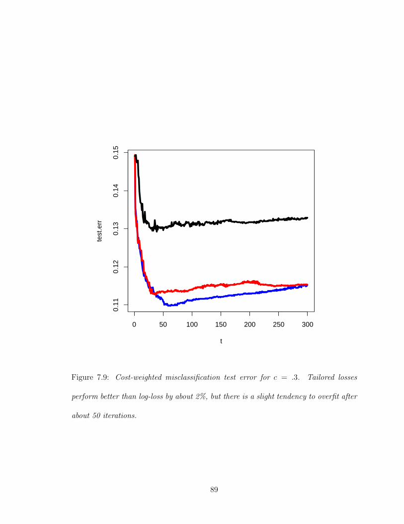
0 50 100 150 200 250 300
0.11
0.12
0.13
0.14
0.15
t
test
.err
Figure 7.9: Cost-weighted misclassification test error for c = .3. Tailored losses
perform better than log-loss by about 2%, but there is a slight tendency to overfit after
about 50 iterations.
89
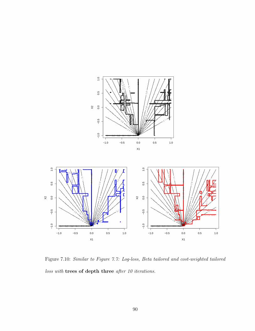
X1
X2
−1.0 −0.5 0.0 0.5 1.0
−1.
0−
0.5
0.0
0.5
1.0
X1
X2
−1.0 −0.5 0.0 0.5 1.0
−1.
0−
0.5
0.0
0.5
1.0
X1
X2
−1.0 −0.5 0.0 0.5 1.0
−1.
0−
0.5
0.0
0.5
1.0
Figure 7.10: Similar to Figure 7.7: Log-loss, Beta tailored and cost-weighted tailored
loss with trees of depth three after 10 iterations.
90
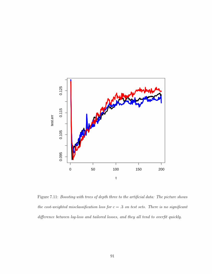
0 50 100 150 200
0.09
50.
105
0.11
50.
125
t
test
.err
Figure 7.11: Boosting with trees of depth three to the artificial data: The picture shows
the cost-weighted misclassification loss for c = .3 on test sets. There is no significant
difference between log-loss and tailored losses, and they all tend to overfit quickly.
91
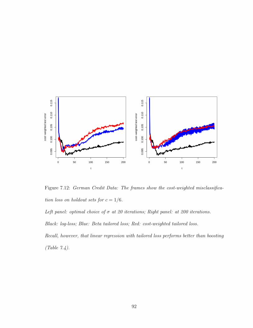
0 50 100 150 200
0.09
50.
100
0.10
50.
110
0.11
5
t
cost
−w
eigh
ted
test
err
or
0 50 100 150 200
0.09
50.
100
0.10
50.
110
0.11
5
t
cost
−w
eigh
ted
test
err
or
Figure 7.12: German Credit Data: The frames show the cost-weighted misclassifica-
tion loss on holdout sets for c = 1/6.
Left panel: optimal choice of σ at 20 iterations; Right panel: at 200 iterations.
Black: log-loss; Blue: Beta tailored loss; Red: cost-weighted tailored loss.
Recall, however, that linear regression with tailored loss performs better than boosting
(Table 7.4).
92
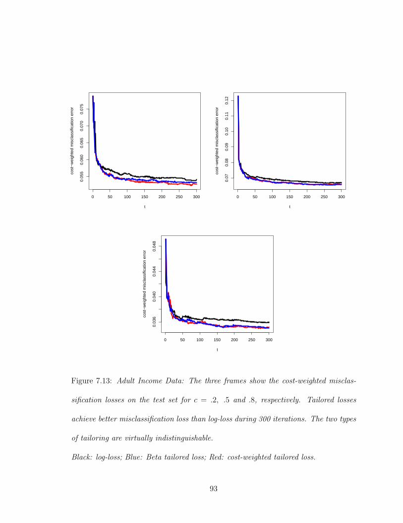
0 50 100 150 200 250 300
0.05
50.
060
0.06
50.
070
0.07
5
t
cost
−w
eigh
ted
mis
clas
sific
atio
n er
ror
0 50 100 150 200 250 300
0.07
0.08
0.09
0.10
0.11
0.12
t
cost
−w
eigh
ted
mis
clas
sific
atio
n er
ror
0 50 100 150 200 250 300
0.03
60.
040
0.04
40.
048
t
cost
−w
eigh
ted
mis
clas
sific
atio
n er
ror
Figure 7.13: Adult Income Data: The three frames show the cost-weighted misclas-
sification losses on the test set for c = .2, .5 and .8, respectively. Tailored losses
achieve better misclassification loss than log-loss during 300 iterations. The two types
of tailoring are virtually indistinguishable.
Black: log-loss; Blue: Beta tailored loss; Red: cost-weighted tailored loss.
93

Chapter 8
Conclusions
This work is concerned with binary classification and class probability estimation.
We described a very general class of loss functions, called F -losses, that can be used
for estimating “uncalibrated probabilities”. An important subset is formed by those
losses that produce calibrated probability estimates; they are known as “proper scor-
ing rules”. General F -losses are compositions of (inverse) link functions and proper
scoring rules. We showed that F -losses are closed under cost-weighting, that is, the
assignment of different weights to the two types of misclassification losses.
We described the known structure of proper scoring rules and showed how the
freedom of choosing among them can be used to tailor fitted models in such a way
that good performance is achieved at a prescribed ratio of misclassification costs.
Similarly, we showed how cost-weighting F -losses can achieve tailoring at given costs.
We also indicated that appropriate degree of tailoring can be estimated from the data
with cross-validation.
94

We gave evidence that tailoring can be of interest in two situations:
1. Tailoring tree-based classifiers to the high or the low end of class 1 probabilities,
thus producing trees with vastly greater interpretability than standard trees
based on the Gini index or entropy.
2. Tailoring to specific classification thresholds when the models are biased for
class probability estimation, yet are capable of describing good classification
boundaries. This case can occur, for example, in linear logistic models when
the sample size is relatively large compared to the number of fitted degrees of
freedom. In such situations it may be beneficial to downweight data points
whose class probabilities are far from the intended threshold. In linear mod-
els, the heavy reliance of log-loss and exponential loss on the most predictable
instances can be a drawback for classification where one cares most about a
specific classification boundary rather than global probability estimation.
Application of tailored losses to more flexible nonparametric models such as boosting
does not achieve similar improvements as in linear models or surprising interpretabil-
ity as in trees.
95

Bibliography
[1] Bregman, L. M. (1967). The Relaxation Method of Finding the Common Point
of Convex Sets and its Applications to the Solution of Problems in Convex Pro-
gramming. U.S.S.R. Computational Mathematics and Mathematical Physics 7
(1), 200–217.
[2] Breiman, L. (1996). Bias, variance and arcing classifiers. Technical Report 460,
Statistics Department, University of California at Berkeley, Berkeley, CA.
[3] Breiman, L., Friedman, J. H., Olshen, R., and Stone, C. J. (1984). Classification
and Regression Trees, Belmont, California: Wadsworth.
[4] Buja, A., and Lee, Y.-S. (2001). Data Mining Criteria for Tree-Based Regression
and Classification, Proceedings of KDD 2001, 27–36.
[5] Clark, L. A., and Pregibon, D. (1992). Tree-Based Models, in Statistical Models
in S, edited by J. M.Chambers and T. J. Hastie, Pacific Grove, CA: Wadsworth
& Brooks/Cole, 377–419.
96

[6] Collins, M., Schapire, R. E., Singer, Y. (2002). Logistic Regression, AdaBoost
and Bregman Distances, Machine Learning, 48 (1/2/3).
[7] Cressie, N. and Read, T. R. C. (1984). Multinomial Goodness-of-fit Tests, J. R.
Statist. Soc. B, 46, No. 3, 440–464.
[8] Domingos, P. (2000). A Unified Bias-Variance Decomposition for Zero-One and
Squared Loss. In: Proceedings of the Seventeenth National Conference on Artifi-
cial Intelligence, 564–569. Austin, TX: AAAI Press.
[9] Elkan, C. (2001). The Foundations of Cost-Sensitive Learning. In: Proceedings of
the Seventeenth International Joint Conference on Artificial Intelligence (IJCAI),
973–978.
[10] Freund, Y., and Schapire, R. (1996). Experiments with a New Boosting Algo-
rithm. In: Machine Learning: Proceedings of the Thirteenth International Con-
ference, 148–156.
[11] Friedman, J. H. (1997). On bias, variance, 0/1 - loss, and the curse-of-
dimensionality. Data Mining and Knowledge Discovery, 1, 55–77.
[12] Friedman, J. H., Hastie, T., and Tibshirani, R. (2000). Additive Logistic Re-
gression: A Statistical View of Boosting, The Annals of Statistics 28, No. 2,
337–407.
97
[13] Garthwaite, P. H., Kadane, J. B., and O’Hagan, A. 2005). Statistical Methods
for Eliciting Probability Distributions, J. of the American Statistical Association,
100, No. 470, 680-700.
[14] Hand, D. J., and Vinciotti, V. (2003). Local Versus Global Models for Classifi-
cation Problems: Fitting Models Where it Matters. The American Statistician
57, No. 2, 124–131.
[15] Kearns, M., and Mansour, Y. (1996). On the boosting ability of top-down de-
cision tree learning algorithms. Proceedings of the Annual ACM Symposium on
the Theory of Computing, 459–468.
[16] Kohavi, R., and Wolpert, D. H. (1996). Bias plus variance decomposition for zero-
one loss functions. In: Proceedings of the Thirteenth International Conference on
Machine Learning, 275–283. Bari, Italy: Morgan Kaufmann.
[17] Kong, E.B., and Dietterich, T.G. (1995). Error-correcting output coding corrects
bias and variance. In: Proceedings of the Twelfth International Conference on
Machine Learning, 313–321. Tahoe City, CA: Morgan Kaufmann.
[18] Lafferty, J. D., Della Pietra S., Della Pietra V. (1997). Statistical Learning Algo-
rithms based on Bregman Distances, in: Proceedings of the Canadian Workshop
on Information Theory 1997.
[19] Lin, Y. (2001) A Note on Margin-based Loss Functions in Classification in Statis-
tics and Probability Letters 68/1. 73-82.
98

[20] Lugosi, G., and Vayatis, N. (2004). On the Bayes-Risk Consistency of Regularized
Boosting Methods, The Annals of Statistics 32, 30-55.
[21] Murphy, A.H. and Daan, H. (1985). Forecast Evaluation, in: Probability, Statis-
tics and Decision Making in the Atmospheric Sciences, eds. Murphy, A.H. and
Katz, P.W.
[22] Quinlan, J.R. (1993). C4.5: Programs for Machine Learning. San Francisco, CA:
Morgan Kaufmann Publishers.
[23] Savage, L.J. (1973). Elicitation of Personal Probabilities and Expectations, J. of
the American Statistical Association 66, No. 336, 783–801.
[24] Schervish, M.J. (1989). A General Method for Comparing Probability Assessors,
The Annals of Statistics 17, No. 4, 1856–1879.
[25] Shuford, E.H., Albert, A., Massengill, H.E. (1966). Admissible Probability Mea-
surement Procedures, Psychometrika 31, 125–145.
[26] Winkler, R.L, (1993). Evaluating Probabilities: Asymmetric Scoring Rules, Man-
agement Science 40, No. 11, 1395–1405.
[27] Schapire, R.E., Singer, Y. (1998). Improved Boosting Algorithms Using
Confidence-Rated Predictions, in Proceedings of the Eleventh Annual Confer-
ence on Computational Learning Theory.
99

[28] Schapire, R.E. (2002). The Boosting Approach to Machine Learning: An
Overview. In: MSRI Workshop on Nonlinear Estimation and Classification.
[29] Tibshirani, R. (1996). Bias, variance and prediction error for classification rules.
Technical report, Department of Preventive Medicine and Biostatistics and De-
partment of Statistics, University of Toronto, Toronto, Canada.
[30] UC Irvine Machine Learning Repository (2003):
http://www.ics.uci.edu/˜mlearn/MLRepository.html
[31] Weisstein, E. W. (2005). Hypergeometric Function. From MathWorld–A Wol-
fram Web Resource.
http://mathworld.wolfram.com/HypergeometricFunction.html
[32] Zhang, T. (2004). Statistical Behavior and Consistency of Classification Methods
based on Convex Risk Minimization. The Annals of Statistics 32, 56-134.
100

Appendix: Proofs
Link function: Recall that F (p) is a minimizer of R(p|F ). Now modify the cost-
weighted F -loss such that the combined coefficients involving c and p add up to one:
Rcw(p|F ) ∼(1− c)p
(1− c)p + c(1− p)L1(−F ) +
c(1− p)
(1− c)p + c(1− p)L0(F )
= R
(
(1− c)p
(1− c)p + c(1− p)
∣
∣
∣
∣
F
)
It follows that the minimizer is
F
(
(1− c)p
(1− c)p + c(1− p)
)
,
hence the link function is
F cw(q) = F
(
(1− c)q
(1− c)q + c(1− q)
)
,
which proves the assertion about the cost-weighted link function.
Proper scoring rule. Plug the new link function into the cost-weighted F -loss and
obtain
Lcw1 (1− p) = (1− c)L1(−F
(
(1− c)p
(1− c)p + c(1− p)
)
) ,
Lcw0 (p) = cL0(F
(
(1− c)p
(1− c)p + c(1− p)
)
) .
Recalling that the original proper scoring rule was L1(1−q) = L1(−F (q)) and L0(q) =
L0(F (q)) and comparing with the above equations, the assertion about the proper
scoring rule follows.
101

Weight function: The third part is obtained from the following calculation:
ωcw(q) =Lcw′
0(q)
q
=c
qL′
0
(
(1− c)q
(1− c)q + c(1− q)
)
(1− c)c
((1− c)q + c(1− q))2
=L′
0
(
(1−c)q(1−c)q+c(1−q)
)
(1−c)q(1−c)q+c(1−q)
(1− c)2c2
((1− c)q + c(1− q))3
= ω
(
(1− c)q
(1− c)q + c(1− q)
)
(1− c)2c2
((1− c)q + c(1− q))3
Normalizing constant: We assume that ω(q) is a density with expectation µ:
∫ 1
0
ω(q) dq = 1 , µ =
∫ 1
0
q ω(q) dq .
The normalizing constant of ωcw(q) is
∫ 1
0
ωcw(q) dq =
∫ 1
0
ω
(
(1− c)q
(1− c)q + c(1− q)
)
(1− c)2c2
((1− c)q + c(1− q))3dq .
The following variable transformation will be used repeatedly in what follows:
t =(1− c)q
(1− c)q + c(1− q), q =
ct
ct + (1− c)(1− t), (8.1)
ωcw(q) dq = [ct + (1− c)(1− t)] ω(t) dt
Thus the normalizing constant is
∫ 1
0
ωcw(q)dq =
∫ 1
0
ω(t) [ct + (1− c)(1− t)] dt = cµ + (1− c)(1− µ) ,
and the following is hence a density:
ωcw(q)
cµ + (1− c)(1− µ). (8.2)
102
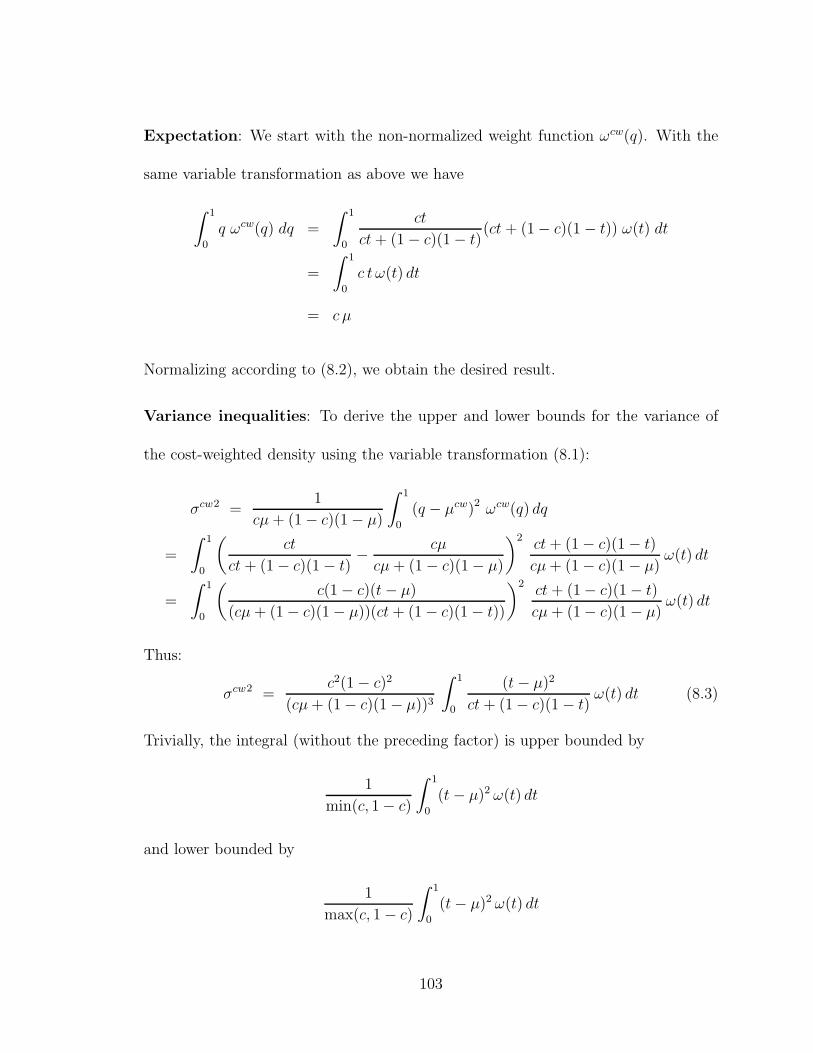
Expectation: We start with the non-normalized weight function ωcw(q). With the
same variable transformation as above we have
∫ 1
0
q ωcw(q) dq =
∫ 1
0
ct
ct + (1− c)(1− t)(ct + (1− c)(1− t)) ω(t) dt
=
∫ 1
0
c t ω(t) dt
= c µ
Normalizing according to (8.2), we obtain the desired result.
Variance inequalities: To derive the upper and lower bounds for the variance of
the cost-weighted density using the variable transformation (8.1):
σcw2 =1
cµ + (1− c)(1− µ)
∫ 1
0
(q − µcw)2 ωcw(q) dq
=
∫ 1
0
(
ct
ct + (1− c)(1− t)−
cµ
cµ + (1− c)(1− µ)
)2ct + (1− c)(1− t)
cµ + (1− c)(1− µ)ω(t) dt
=
∫ 1
0
(
c(1− c)(t− µ)
(cµ + (1− c)(1− µ))(ct + (1− c)(1− t))
)2ct + (1− c)(1− t)
cµ + (1− c)(1− µ)ω(t) dt
Thus:
σcw2 =c2(1− c)2
(cµ + (1− c)(1− µ))3
∫ 1
0
(t− µ)2
ct + (1− c)(1− t)ω(t) dt (8.3)
Trivially, the integral (without the preceding factor) is upper bounded by
1
min(c, 1− c)
∫ 1
0
(t− µ)2 ω(t) dt
and lower bounded by
1
max(c, 1− c)
∫ 1
0
(t− µ)2 ω(t) dt
103
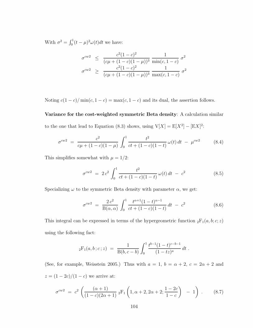
With σ2 =∫ 1
0(t− µ)2ω(t)dt we have:
σcw2 ≤c2(1− c)2
(cµ + (1− c)(1− µ))3
1
min(c, 1− c)σ2
σcw2 ≥c2(1− c)2
(cµ + (1− c)(1− µ))3
1
max(c, 1− c)σ2
Noting c(1− c)/ min(c, 1− c) = max(c, 1− c) and its dual, the assertion follows.
Variance for the cost-weighted symmetric Beta density: A calculation similar
to the one that lead to Equation (8.3) shows, using V[X] = E[X2]− [EX]2:
σcw2 =c2
cµ + (1− c)(1− µ)
∫ 1
0
t2
ct + (1− c)(1− t)ω(t) dt − µcw2 (8.4)
This simplifies somewhat with µ = 1/2:
σcw2 = 2 c2
∫ 1
0
t2
ct + (1− c)(1− t)ω(t) dt − c2 (8.5)
Specializing ω to the symmetric Beta density with parameter α, we get:
σcw2 =2 c2
B(α, α)
∫ 1
0
tα+1(1− t)α−1
ct + (1− c)(1− t)dt − c2 (8.6)
This integral can be expressed in terms of the hypergeometric function 2F1(a, b; c; z)
using the following fact:
2F1(a, b ; c ; z) =1
B(b, c− b)
∫ 1
0
tb−1(1− t)c−b−1
(1− tz)adt .
(See, for example, Weisstein 2005.) Thus with a = 1, b = α + 2, c = 2α + 2 and
z = (1− 2c)/(1− c) we arrive at:
σcw2 = c2
(
(α + 1)
(1− c)(2α + 1)2F1
(
1, α + 2, 2α + 2;1− 2c
1− c
)
− 1
)
. (8.7)
104

Shape of the cost-weighted symmetric Beta: For the symmetric Beta family,
ωcw(q) is
ωcw(q) ∼qα−1(1− q)α−1
((1− c)q + c(1− q))2α+1
We derive the stationary point of the function as follows: Set ωcw′
(q) = 0 and note
that
(
qα−1(1− q)α−1)′
= (α− 1)(1− 2q)(q(1− q))α−2,
(
((1− c)q + c(1− q))2α+1)′
= (2α + 1)(1− 2c)((1− c)q + c(1− q))2α
Thus the stationarity condition becomes
(α− 1)(1− 2q)(q(1− q))α−2((1− c)q + c(1− q))2α+1
− (2α + 1)(1− 2c)(q(1− q))α−1((1− c)q + c(1− q))2α = 0
which can be simplified to
3(1− 2c)q2 − (α− (6c− 2))q + (α− c)c = 0 .
Solving this equation we get the stationary points
−(α− 2(3c− 1))±√
(α− 2(3c− 1))2 + 12(α− 1)c(2c− 1)
6(2c− 1)
Rewrite this expression as
−((α − 1)− 3(2c− 1))±√
(α− 1)2 + 6(2c− 1)2(α− 1) + 9(2c− 1)2
6(2c− 1)
=−((α− 1)− 3(2c− 1))±
√
(α− 1)2 + 3(2α + 1)(2c− 1)2
6(2c− 1)
105

Notice for α > 1, the weight function has a unique mode at
−(α − 2(3c− 1)) +√
(α− 2(3c− 1))2 + 12(α− 1)c(2c− 1)
6(2c− 1)
The other stationary point is outside the [0, 1] interval.
For α < 1, the weight function has a unique minimum at
−(α− 2(3c− 1))−√
(α− 2(3c− 1))2 + 12(α− 1)c(2c− 1)
6(2c− 1)
The other stationary point is out of bound.
For α = 1 and c 6= 0.5, the weight function has a unique mode and maximum at
0 or 1.
106