loss aversion and learning to bid

Loss Aversion and Learning to Bid

By DENNIS A. V. DITTRICH†, WERNER GUTH‡, MARTIN G. KOCHER§ andPAUL PEZANIS-CHRISTOU¶

†Jacobs University, Bremen ‡Max Planck Institute of Economics §University of Munich

¶BETA, Universite de Strasbourg

Final version received 23 February 2011.

Bidding challenges learning theories. Even with the same bid, experiences vary stochastically: the same

choice can result in either a gain or a loss. In such an environment, the question arises of how the nearly

universally documented phenomenon of loss aversion affects the adaptive dynamics. We analyse the

impact of loss aversion in a simple auction using the experienced-weighted attraction model of learning.

Our experimental results suggest that individual learning dynamics are highly heterogeneous and affected

by loss aversion to different degrees. Apart from that, the experiment shows that loss aversion is not

specific to rare decision-making.

INTRODUCTION

There are very rare situations where bidding games—usually referred to as auctions—aredominance solvable, like in the random price mechanism (see Becker et al. 1964) or insecond-price auctions (see Gandenberger 1961; Vickrey 1961). Apart from such specialsetups, bidding poses quite a challenge for learning. According to the usual first-price rule(the winner is the highest bidder, and she pays her bid to buy the object), one has tounderbid one’s own value (bid shading) to guarantee a positive profit in case of buying.Such underbidding may cause feelings of regret or loss when the object has not beenbought, although its price was lower than one’s own value. Similarly, even on winningthe auction, feelings of loss may be evoked since one could have won more by a lowerbid. When the values of the interacting bidders are stochastic, whether one experiences aloss or a gain is highly stochastic.

In this paper we investigate two important issues. First, we reassess the issue of learn-ing in auctions. Although bidding experiments are numerous in economics (see Kagel1995 for an early survey), hardly any of them provide as much opportunity for learningas we do (see, for example, Garvin and Kagel 1994; Selten and Buchta 1998; Armantier2004; Guth et al. 2003). We believe that the number of repetitions in most studies hasbeen too low to fully account for possible learning dynamics. In stochastic environments,learning is typically slow, and the number of repetitions or past bidding experiences areimportant dimensions. Our one-bidder contest (Bazerman and Samuelson 1983; Ballet al. 1991) allows for a considerable number of repetitions. To directly identify the path-dependence of bidding behaviour (i.e. why and how bidding behaviour adjusts in the lightof past results) without any confounding factors, we deliberately choose a bidding taskthat lacks strategic interaction.

We analyse the learning dynamics by estimating the parameters of several variants ofHo et al.’s (2007) experienced weighted attraction (EWA) learning model. The EWAlearning model is a hybrid of reinforcement and belief models that uses informationabout forgone payoffs as well as past choice behaviour. Either information would beignored by pure reinforcement or pure belief learning. Estimating best-fitting parametervalues for the EWA learning model thus effectively allows us to compare a large number

© 2011 The London School of Economics and Political Science. Published by Blackwell Publishing, 9600 Garsington Road,

Oxford OX4 2DQ, UK and 350 Main St, Malden, MA 02148, USA

Economica (2012) 79, 226–257

doi:10.1111/j.1468-0335.2011.00892.x

of different learning models in one go. We are interested in the individual behaviour,which we expect to be heterogeneous with respect to the underlying parameters of theEWA model. Consequently, we estimate the parameters for each participant separatelyand discuss the distribution of estimated parameters.

Second, we experimentally test for the impact of loss aversion (Kahneman and Tver-sky 1979; Tversky and Kahneman 1992) on the learning dynamics in this bidding task byincorporating a loss parameter in the EWA learning model. Loss aversion is referred toas the behavioural tendency of individuals to weigh losses more heavily than gains; thereis ample evidence for loss aversion in both risky and risk-free environments (see Starmer2000 for an overview). In our setup, we avoid the possible ambiguity of the referencepoint implied by loss aversion: losses are monetary losses compared to no-trading. Obvi-ously, in a first-price auction all possible choices can prove to be a success (yield a gain)or a failure (imply a loss), at least in retrospect. Therefore the usual and robust finding ofloss aversion should be reflected in the adaptation dynamics.

More specifically, we distinguish losses from bidding and hypothetical—i.e. non-real-ized—retrospective gains from not bidding as both shape the future attraction of bidding.In doing so we can reasonably exclude idiosyncratic risk attitudes, since due to cumula-tive payments (over 500 rounds), the variance of total earnings should be close to zero.Our main hypothesis on the impact of loss aversion claims that in absolute terms, anactual loss will change bidding dispositions more than an equally large gain. To the bestof our knowledge, loss aversion has so far received little attention (one example, consider-ing only hypothetical losses, is Ockenfels and Selten 2005) when specifying learningdynamics in situations comparable to ours. Note that—since risk aversion might disap-pear when playing many rounds due to diversification—one could expect that the so fardocumented confirmation of loss aversion might also be specific to rare decision-making.

In the basic bidding task (originally studied experimentally by Samuelson and Bazer-man (1985), and more recently by Selten et al. (2005) and Charness and Levin (2009)) towhich subjects are exposed in our experiment, the only bidder and the seller have per-fectly correlated values. Put differently, the seller’s valuation is always the same constantand proper share of the bidder’s value. Whereas the seller knows her value, the bidderknows only how it is randomly generated.

The bid of the potential buyer determines the price if the asset is sold. In our experi-ment (as in earlier studies) the seller is captured by a robot strategy, accepting only bidsexceeding her evaluation. Thus the bidder has to anticipate that whenever her bid isaccepted, it must have exceeded the seller’s valuation. Neglecting this fact may cause thewinner’s curse as in standard common-value auctions involving more than one bidder.

If the seller’s share or quota in the bidder’s value is high, i.e. when the positive surplusis relatively low, such a situation turns out to be a social dilemma: according to the solu-tion under risk neutrality,1 the bidder abstains from bidding in spite of the positivesurplus for all possible values. However, if the quota is low, the surplus is fully exploited:the optimal bid exceeds the highest valuation of the seller and thereby guarantees trade.Earlier studies have focused only on the former possibility. In our experiment each parti-cipant, as bidder, repeatedly experiences both low and high quotas. It is straightforwardthat the bidding tasks to which participants are exposed constitute an ideal environmentin which to study learning because other, possibly confounding behavioural determinantssuch as the effects of social preferences are non-existent.

When bids can vary continuously, it is rather tricky to explore how bidding behaviouris adjusted in the light of past results. Traditional learning models like reinforcementlearning—also referred to as stimulus–response dynamics or law of effect (see Bush and

Economica

© 2011 The London School of Economics and Political Science

2012] LOSS AVERSION AND LEARNING TO BID 227

Mosteller 1955)—cannot readily be applied. Therefore we offered participants only abinary choice, namely to abstain from or to engage in bidding. In order to observe directlythe inclination to abstain or engage, respectively, we allowed participants to explicitlyrandomize their choice among the two possible strategies. (For earlier experimentsoffering explicitly mixed strategies, see, for example, Ochs 1995; Anderhub et al. 2002.)

In retrospective analysis, both situations where bidders should abstain from orengage in trade will render both choices as good and as bad with positive probability.If restricted to binary choices, a bidder’s (un)willingness to engage in trade could bedetected by comparing behaviour in different rounds of the same game. This, however,would interfere with learning, which we expect to be relevant. Allowing for mixing is away to elicit (un)willingness to trade without confounding it with learning. Will loss aver-sion be equally strong for a bidder who has chosen probability 1 and one who came tothe same choice by implementing proper mixing? If not, our experiment would serve as aparticularly challenging setup for observing loss aversion, and, thus it would even corrob-orate any confirmation of loss aversion effects. Another justification for the use of explicitmixed strategies is that in a binary choice protocol we could never be sure whether parti-cipants randomly determine their choice behaviour, and if they randomize the probabili-ties that they assign to the available pure strategies. Offering explicit random devicestherefore implies a better control of individual decision-making.

More specifically, each participant played 250 rounds each of both the same high-quota and same low-quota game, where a low quota suggests an efficient benchmarksolution and a high quota an inefficient one. As mentioned earlier, we consider suchextensive experience necessary since learning in stochastic settings is typically slow.We also wanted sufficiently many loss and gain experiences for each participant when try-ing to explore the path-dependence of bidding behaviour and how adaptation is influ-enced by loss aversion.

As our analysis of the data shows, learning in the experiment is indeed slow; half ofthe subjects seem not to learn using the payoff-maximizing strategies within the givennumber of rounds. According to the EWA learning model, observed learning is charac-terized by a long memory, and participants do not discount past experiences. This isreasonable given that even though the bidding task is highly stochastic, it remains stablethroughout the experiment. Retrospective gains and losses have a slightly more hetero-geneous impact on the learning dynamics. Even so, the majority of participants attachconsiderable importance to retrospective gains and losses. With respect to loss aversionwe observe a substantial degree of heterogeneity in our data. Although the majority ofparticipants put a higher weight on losses than on gains, there are a few participantswho discount losses. Nonetheless, allowing for loss aversion significantly improves thegoodness-of-fit of the EWA learning model.

The paper proceeds as follows. The next section introduces the basic model in its con-tinuous and binary forms. In Section II we discuss the details of the experimental designand the laboratory protocol. Section III presents the experimental data. In Section IV wediscuss experience-weighted attraction learning and loss aversion. We estimate severallearning functions for our experiment participants and assess the importance of losses intheir learning behaviour. Section V concludes.

I. THE MODEL

Before introducing the binary bidding task, let us briefly discuss its continuous version.Let v denote the value of an asset to be sold by a seller. This value is randomly drawn

Economica


228 ECONOMICA [APRIL

from a uniform distribution defined on [0,100] and is unknown to the bidder; the latterknows only how it has been generated. The seller knows v but has an evaluation that isequal to qv, with q ∈ (0, 1] and q 6¼ 0.5. She agrees to sell the asset only if the bidder’sbid satisfies b [ qv. The value of q is known to both the seller and the bidder.

Since a risk-neutral buyer earns v � b when b [ qv (or v\ b/q) and 0 otherwise, herexpected payoff takes the following form:

Eðv� bÞ ¼R b=q

0 ðv� bÞ 1100

dv ¼ b2

100q12q

� 1� �

for 0� b� 100q;R 100

0 ðv� bÞ 1100

dv ¼ 50� b for 100q\b\100:

8<:ð1Þ

The first expression stands for the bidder’s expected payoff when submitting a bidsmaller than 100q, the seller’s highest possible evaluation of the asset. The second expres-sion stands for the expected payoff when submitting a bid greater than this maximumpossible evaluation.2

It follows from equation (1) that any positive bid b � 100q implies a positiveexpected profit if q\ 0.5. Thus the optimal bid b� depends on q via

b� ¼ b�ðqÞ ¼ 100q for 0\ q\ 0:5,0 for 0:5\ q\ 1,

�ð2Þ

so that Eðv� b�Þ ¼ 50� 100q for 0\ q\ 0.5 and 0 for 0.5\ q\ 1. In the caseq [ 0.5, the positive expected surplus of

Z 100

0

ð1� qÞ 1

100v dv ¼ 50ð1� qÞð3Þ

is lost, whereas in case of q\ 0.5 it is fully exploited.The binary version of this game assumes only two possible bids, 0 and B, instead of

all bids in [0,100]. In our experiments, all participants repeatedly encounter two biddingenvironments: one with 0\ q\ 0.5 for which it is optimal to bid B, and one with0.5\ q\ 1 for which it is optimal to bid 0. In both environments, participants have tochoose between bidding 0 and bidding B (by assigning a weighing probability—see thenext section). We further assume that 0\ B\ 100 so that bidding B does not warranttrade and thus efficiency.

Let us finally investigate the stochastic payoff effects for bidding 0 or B. By biddingb = 0, the bidder never buys. However, as the asset’s value v is revealed after the sale,she should understand that compared to b = B, her previous bid b = 0 is retrospectivelyjustified if B [ v, which happens with probability Pþ

0 ¼ B=100. On the other hand, ifv [ B [ qv, which happens with probability P�

0 ¼ B=ð100qÞ � B=100, having bid b = 0counts as a loss of v � B in retrospect.

For b = B, if no trade takes place (because qv [ B, occurring with probabilityPn0 ¼ 1� ðB=ð100qÞÞ), then there is no retrospective feeling of a loss or a gain. Similarly,

b = B implies a gain of v � B if v [ B [ qv, which happens with probability PþB ¼

B=ð100qÞ � B=100, and a loss of v � B if B [ v, which occurs with probabilityP�B ¼ B=100. There is no trade whenever qv[B, which happens with probability

PnB ¼ 1� ðB=ð100qÞÞ. The assumption 0\B\ qð1þ qÞ�1 guarantees that all probabili-

ties Pþ0 ¼ P�

B , P�0 ¼ Pþ

B and Pn0 ¼ Pn

B ¼ Pn are positive. To summarize, regardless ofwhether q = q or q ¼ �q applies, the gains and losses associated to bidding b = B areactual, whereas those associated to bidding b = 0 are retrospective.

Economica



II. LABORATORY PROTOCOL

Participants were instructed that there are two roles, and they would act as buyers withthe computer acting as the seller by following a fixed robot strategy. The instructionsinformed participants about parameter values, the distribution of the values, and the rulefollowed by the robot seller.3

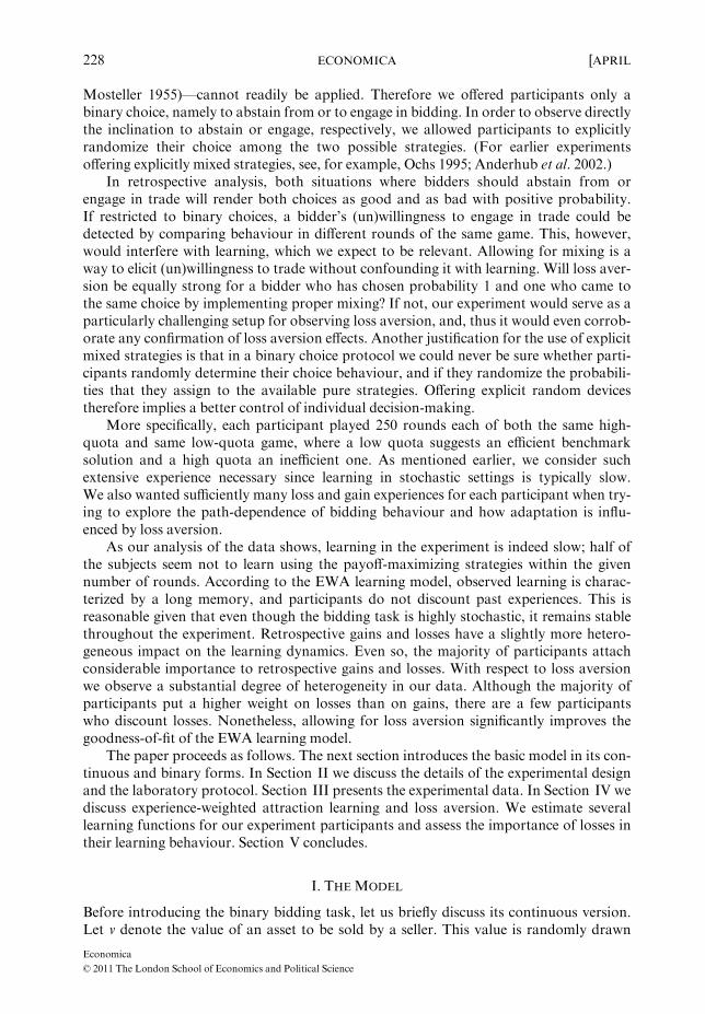
We chose B = 25, q = 0.4 and �q ¼ 0:6. For such parameters and assuming risk-neu-trality, it is optimal to bid b = B when q = 0.4 and to bid b = 0 when q = 0.6. We reportin Figure 1 the bidder’s expected profits for each value of q.

To observe the bidders’ propensities Pt for bidding B, we asked them to assign aprobability of submitting a bid B on an 11-point scale ranging from 0% to 100% with astep size of 10 percentage points. Therefore the pure strategies of bidding 0 or B areequivalent to a choice of 0% or 100% on the 11-point probability scale; of course, wedid not impose a default option for the mixed strategy choice, in order not to influencesubjects in any way.4 One of the advantages of such a method is that it avoids the experi-mentally uncontrolled randomness of a binary choice between bidding bt ¼ 0 and bt ¼ Bwhen checking, for each individual participant, how well a postulated adaptive processcaptures her idiosyncratic learning behaviour.

While the feeling of loss aversion is probably less important when submitting bids bychance, we conjecture that the variety of situations encountered over a long sequence ofplay should ensure its salience in subjects’ behaviour.5 Note further that no subject in ourexperiment consistently determined his or her bid completely by chance, and that purestrategy choices were rather frequent.

In spite of the 500 rounds of play, the whole experiment took less than two hours tocomplete, including the time needed to read the instructions. As already mentioned, weallowed for a sufficiently large number of repetitions to be able to test for learning effectssince the assessment of loss aversion in a stochastic environment requires many repeti-tions. At the end of each round t, participants were informed about the value vt, whethertrade occurred or not, and about earnings for both possible choices, i.e. for bt ¼ B andbt ¼ 0. The values q = 0.4 or q = 0.6 were displayed on each decision screen and alter-nated every ten rounds.

The conversion rate from experimental points to euros (1:200) was announced in theinstructions. Participants received an initial endowment of 1500 experimental points(€7.50) to avoid bankruptcy during the experiment. As a matter of fact, such a case never

0

–50

–30

–10

10

Exp

ecte

d pr

ofits

q = 0.4q = 0.6

20 40Bid b

60 80 100

FIGURE 1. Expected profits for each bid b under the experimental conditions.

Economica



occurred. Average earnings were €10.56 (with standard deviation 1.3). Overall, 42 sub-jects participated in the two sessions that we conducted. The experiment was computer-ized using z-Tree (Fischbacher 2007) and was conducted with students of the Universityof Jena.

III. DESCRIPTIVE RESULTS

We start by presenting some descriptive results on subjects’ behaviour before assessingthe extent of loss aversion within a learning framework.

Decision time

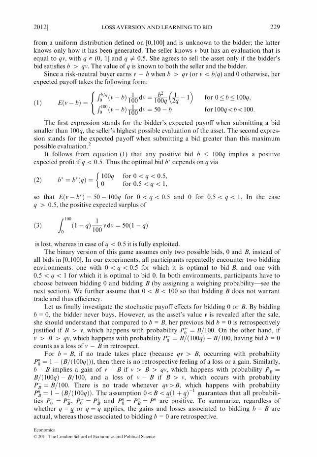
Since an experiment with 500 rounds of play is rather long, our first concern is nat-urally whether participants remained cognitively active during the whole experiment.In particular, boredom could induce subjects to no longer consider the available infor-mation and to no longer adjust their behaviour accordingly. Although we cannotexclude that some subjects got bored by the experiment, there are several indicationsthat this was not at all predominant: Figure 2 shows the average decision time (in sec-onds) over the 500 rounds of play. The average decision time is the longest (about490 seconds) in the first period, and it declines as the experiment proceeds. Byround 80 the average decision time falls below 5 seconds, and it reaches 3.5 secondsin the last period.

We also observe periodic spikes in the average decision time until the very end.As most spikes occur at a q-regime switch, their presence suggests that participants con-sidered the new information displayed on their screens. The average increase in decisiontime after a regime switch is about 30%, and the difference is highly significant(p\ 0.001, according to a Wald test using the results of a model that controls forrepeated measurements). After the last regime switch (at round 490), the increase in deci-sion time is about 67% (one-sided t-test, p = 0.030).

Eventually, we take the subjects’ positive comments and reactions at informal end-of-session debriefings as evidence that they did not get bored by the experiment.

0

0

10

20

30

40

Period

Seco

nds

100 200 300 400 500

FIGURE 2. Average decision time.

Note: The shaded area covers the actual decision time in each period for all participants.

Economica



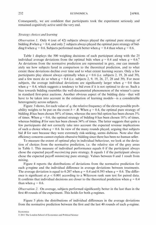
Consequently, we are confident that participants took the experiment seriously andremained cognitively active until the very end.

Strategy choices and learning

Observation 1. Only 4 (out of 42) subjects always played the optimal pure strategy ofbidding Bwhen q = 0.4, and only 2 subjects always played the optimal pure strategy of bid-ding 0 when q = 0.6. Subjects performed much better when q = 0.4 than when q = 0.6.

Table 1 displays the 500 weighing decisions of each participant along with the 25individual average deviations from the optimal bids when q = 0.4 and when q = 0.6.6

As deviations from the normative prediction are represented in grey, one can immedi-ately see how subjects fared in comparison to the theoretical prediction, and to whatextent these deviations decline over time and to what extent learning occurs. Only a fewparticipants play almost always optimally when q = 0.6 (i.e. subjects 2, 19, 26 and 39),and a few more do so when q = 0.4 (i.e. subjects 2, 9, 19, 26, 27, 28 and 39). For mostsubjects, the average individual deviations are significantly larger when q = 0.6 thanwhen q = 0.4, which suggests a tendency to bid even if it is not optimal to do so. Such abias towards bidding resembles the well-documented phenomenon of the winner’s cursein standard first-price auctions. Another obvious aspect of the bidding data—that willhave to be taken into account in the estimation of learning models—is a considerableheterogeneity across subjects.

Figure 3 shows, for each value of q, the relative frequency of the eleven possible prob-ability weights to be put on the event b = B. When q = 0.4, the optimal pure strategy ofbidding B has been chosen 58% of times, whereas the zero bid option has been chosen 3%of times. When q = 0.6, the optimal strategy of bidding 0 has been chosen 18% of times,whereas bidding B for sure has been chosen 34% of times. The latter suggests that quite afew participants did not correctly take into account the expected revenue implicationsof such a choice when q = 0.6. In view of the many rounds played, arguing that subjectsbid B for sure because they were extremely risk-seeking, seems dubious. Note also thatefficiency concerns cannot explain obsessive bidding since there has been no human seller.

To measure the extent of optimal play in individual behaviour, we look at the devia-tion of choices from the normative prediction, i.e. the relative size of the grey areasin Table 1. This measure of individual performance equals 0 if the participant alwayschose the expected payoff maximizing pure strategy. It equals 1 if the participant alwayschose the expected payoff minimizing pure strategy. Values between 0 and 1 result frommixing.

Figure 4 reports the distributions of deviations from the normative prediction foreach q-regime and the individual difference in average deviations between treatments.The average deviation is equal to 0.207 when q = 0.4 and 0.593 when q = 0.6. The differ-ence is significant at p\ 0.001 according to a Wilcoxon rank sum test for paired data.It confirms that individual decisions are closer to the theoretical prediction when q = 0.4than when q = 0.6.

Observation 2. On average, subjects performed significantly better in the last than in thefirst 40 rounds of the experiment. This holds for both q-regimes.

Figure 5 plots the distributions of individual differences in the average deviationsfrom the normative prediction between the first and the last 40 rounds of each q-regime.

Economica



TABLE 1CHOICES AND DEVIATIONS FROM THE NORMATIVE PREDICTION

Mean deviationChoicesSubject

ID 1 Round 500 q q

123456789101112131415161718192021222324252627282930313233343536373839404142

NotesBlack dots represent actual choices during the 500 rounds; grey bars are deviations from the normative solution.Mean deviations from the normative solution in columns three and four are computed for each block of tenrounds under the respective q-regime. While a point at the bottom of a line indicates bidding with probability 0,a point at the top of a line indicates bidding with probability 1. The subject is closer to the normative solutionthe more white space the graph shows.Subject 19 exceeded the time limit and had to stop after only 400 rounds.

Economica



A negative difference indicates a reduction in deviations from the normative predictionover time and suggests that learning occurred over the course of the experiment. Accord-ing to this measure, 22 participants moved towards the normative prediction whenq = 0.4, and 23 when q = 0.6. Similarly, 14 participants moved away from the normativeprediction when q = 0.4, and 15 when q = 0.6. On average, the participants’ deviationsdecreased by 5 percentage points between the first and the last 40 rounds when q = 0.4(t-test, p = 0.035) and by 9 percentage points when q = 0.6 (p = 0.043). Overall, 29participants ‘learned’ the normative solution, and deviations decreased by 7 percentagepoints (p = 0.003).

In the last 100 rounds of play, 24% of participants (10 bidders) always played theoptimal strategy when q = 0.4, and 10% of the participants (4 bidders) did so whenq = 0.6. The latter outcome is in line with the 7% reported by Ball et al. (1991) for a gamethat corresponds to an environment where q = 0.6, which spanned over 20 rounds andfor which no significant change in behaviour was found. Nevertheless, as only fourbidders use the optimal strategy with q = 0.4 and q = 0.6, the well-documented pattern ofthe winner’s curse is still very present. This result corroborates the findings of Selten et al.(2005) and Charness and Levin (2009), who also found this pattern to be persistent after100 or 60 rounds of play, even in treatments designed to simplify subjects’ bidding task.

Observation 3. Revenues of bidders are higher under q = 0.4 than under q = 0.6. Manybidders fall prey to the winner’s curse under q = 0.6.

As expected, average earnings are also different across q-regimes: they are equal to825.76 points when q = 0.4 (s.d. 223.96, Min 269, Max 1274) and to �213.66 points whenq = 0.6 (s.d. 127.99, Min �547, Max 20).

IV. EWA LEARNING WITH(OUT) LOSS AVERSION

The situation faced by our participants in the experiment poses quite a challenge forlearning theories. Obviously, whatever the bidder chooses, she can retrospectively experi-ence both an encouragement and a regret with positive probability. As already men-tioned, we are interested in two specific questions:

1. Will regret be more decisive than positive encouragement as suggested by (myopic)loss aversion (Benartzi and Thaler 1995; Gneezy and Potters 1997)?

2. Will learning bring about an adjustment to bidding b = B when q = q and b = 0when q ¼ �q ?

In general, reinforcement learning relies on the cognitive assumption that what hasbeen good in the past, will also be good in the future. In such a context, one does not haveto be aware of the decision environment except for an implicit stationarity assumptionjustifying that earlier experiences are a reasonable indicator of future success. In oursetup, actual as well as retrospective gains and losses can be derived unambiguously sincethe bidder is informed about the true value vt after each round t, regardless of whetherthe object has been bought or not.

Ho et al. (2007) propose a one-parameter adaptive experience-weighted attraction(EWA) learning model that takes into account both past experience and expectationsabout the future. It nests reinforcement and belief learning, and can predict the path-dependence of individual behaviour in any normal-form game. Camerer (2003) shows

Economica



Freq

uenc

y

0.0

2

4

6

8

10

0

AD (q = 0.4)

Mean 0.207Median 0.161

0.2 0.4Average deviation

0.6 0.8 1.0

2

4

6

8

10

0

AD (q = 0.6)

Mean 0.593Median 0.656

0.0 0.2 0.4Average deviation

0.6 0.8 1.0

2

4

6

8

10

0

Mean - 0.386Median - 0.406

−1.0Individual difference in averagedeviations between treatments

0.0

AD (q = 0.4) - AD (q = 0.6)

−0.5 0.5

FIGURE 4. Distributions of deviations from payoff maximizing bids.

q = 0.4, AD (t > 460) - AD (t < 41)

Freq

uenc

y

0

2

4

6

8

10

12

–1.0Change in average deviation

Mean - 0.052

0.0–0.5 0.5

q = 0.6, AD (t > 460) - AD (t < 41)

0

2

4

6

8

10

12

Mean - 0.091


0.0–0.5 0.5

AD (t > 460) - AD (t < 41)

0

2

4

6

8

10

12

Mean - 0.072


0.0–0.5 0.5

FIGURE 5. Difference in average deviations from the normative prediction between first and last 40 rounds

for both treatments.

0

q = 0.4q = 0.6

10Probability of bidding in percent20 30 40 50 60 70 80 90 100

0.0

0.2

0.4R

elat

ive

freq

uenc

y 0.6

FIGURE 3. Relative frequency of probability choices.

Economica



that EWA has a better (predictive) fit than pure reinforcement and pure belief learning(and quantal response as a no-learning benchmark) in a number of games. He notes,however, that identification of EWA parameters requires a substantial number of peri-ods. Ho et al. (2007) claim that the EWA learning model can easily be extended to gameswith incomplete information.

In the following, we describe how we incorporated loss aversion in the EWA learningmodel for our game of incomplete information. Denote a bidder’s jth choice by s j, theround t choice by st, and the payoff from choice s j by p j. Let I(·,·) be an indicator func-tion that is equal to 1 if the arguments are equal, and 0 otherwise. Using the notation ofHo et al. (2007), a bidder’s attraction Aj

t for choice j at time t can be defined as

Ajt ¼

/Nt�1Ajt�1 þ ½dþ ð1� dÞIðs j; stÞ�p j

t

Nt�1/ð1� jtÞ þ 1;ð4Þ

whereNt ¼ Nt�1/ð1� jtÞ þ 1 andN0 ¼ 1. Here, the parameter / reflects profit discount-ing or, equivalently, the decay of previous attractions owing to either forgetting or delib-erate discounting of past experience when the learning environment is changing. Thisparameter will be freely estimated, as in the original EWA model of Camerer and Ho(1999). The parameter d stands for the weight placed on retrospective gains and losses(foregone payoffs). A parameter value of d = 0 reduces the EWA learning model to apure reinforcement model. On the other hand, being fully responsive to foregone payoffs,i.e. d = 1, means that the decision-maker’s behaviour is not only reinforced but ratherdriven by a thorough cognitive retrospective analysis of behaviour.

Ho et al. (2007) proposed to tie the decay of attraction to the weight on foregonepayoffs: / = d. They argue that a subject whose behaviour is driven by a thorough cogni-tive retrospective analysis is also more likely not to discount past experiences in a stableenvironment. We estimate models where we place different restrictions on d to analysethe implications of the assumptions of pure reinforcement and pure belief learning, aswell as to test whether the heuristic simplification of Ho et al. (2007) is justified withinour stochastic, yet stable bidding framework.

Finally, j controls the growth rate of attraction. A value of j = 0 implies that attrac-tions will be averaged, while a value of j = 1 implies that attraction will be cumulated.

Ho et al. (2007) argue that if in the past a subject often changed her strategy, she will bemore likely to change her strategy now, given the same feedback. This can be reflected inthe model by letting j be equal to a normalized Gini coefficient on choice frequencies.In our estimations we focus on average attraction under pure reinforcement and pure belieflearning, i.e. we restrict j = 0. Furthermore, we estimate the EWA model as proposedby Ho et al. (2007), and compute the normalized Gini coefficient on choice frequenciesfor each q-regime and period t separately in order to use this variable in place of jt.

In our analysis, the attraction Ajt is calculated only for the binary choice of bidding

B or not bidding. We need to compute only ABt ; the attraction of not bidding is always

zero because the payoff for not bidding is always zero. The mapping of the attractionAB

t to the mixed strategies via a probabilistic choice function is defined in the nextsection.

To augment the standard model by loss aversion, we introduce a loss weight l, andwe define by wt the actual losses and non-realized, retrospective gains in round t, depend-ing on whether bidding B generated a loss or bidding 0 left some money on the table:

wt ¼ q0t ðvt � BÞ þ qBt ðB� vtÞ;ð5Þ

Economica



where q0t ¼ 1 if vt [B[ qvt and b = 0, and q0t ¼ 0 otherwise, and similarly, qBt ¼ 1 ifB[ vt and b = B, and qBt ¼ 0 otherwise.

The bidder’s attraction ABt for the binary choice of bidding b = B in round t then

becomes

ABt ¼ /Nt�1A

Bt�1 þ ½dþ ð1� dÞIðsB; stÞ�½pBt þ lwt�

Nt�1/ð1� jtÞ þ 1:ð6Þ

With such a specification, a loss weight of l = 0 indicates that losses influence the attrac-tion of choosing b = B to the same extent as gains. While a loss weight of l = �1 indicatesthat losses have no influence on the attraction, a loss weight of l = 1 means that lossesinfluence the attraction of choosing b = B by twice the extent of gains.

Estimation procedure

Learning models such as those considered here are models of individual behaviour. Yetmost econometric tests of these models report aggregate parameters that have been esti-mated from individual behaviour in interactive games. While such estimates often suggesta behaviour that is consistent with some kind of reinforcement learning, they typically donot illustrate the extent of heterogeneity in subjects’ behaviour. For our analysis of lossaversion it is thus important to note that, for example, Johnson et al. (2006) provideempirical evidence that individual loss aversion is heterogeneous. Additionally, usingMonte Carlo simulations, Wilcox (2006) shows that there exists a strong estimation biasif players are heterogeneous but a homogeneous representative agent model is estimated.We therefore estimate our models separately for each participant and discuss the distribu-tions of the estimated parameters.7 For reasons of comparability, we also report the esti-mation outcomes of a model that assumes a representative agent and includes the datafrom all participants, comparable to the model used in Ho et al. (2008) based on centi-pede game data from Nagel and Tang (1998).

In the tradition of reinforcement learning models, the attraction ABt for the binary

decision to bid B in period t is assumed to determine the probabilistic choice behav-iour (see Bush and Mosteller 1955; Roth and Erev 1998; Camerer and Ho 1999).Since we allow explicit mixing of the two pure strategies bidding B = 25 and not bid-ding, we need to map the attraction AB

t to the eleven available mixed strategies. Themixed strategies follow a natural order given by their respective probability of submit-ting the bid. Consequently, the mapping of the attraction AB

t to the mixed strategiescan be achieved by an ordinal multinomial choice model (see Agresti 2010). If thenatural order of the mixed strategies were not obvious to our participants, an alterna-tive modelling approach would include computing separate attractions for each avail-able mixed strategy and mapping them to choices via an unordered multinomialchoice model.8

We choose the ordered logit model for the mapping of attraction to choices. Let s� bea single latent variable with

s�t ¼ b1Iðqt; qÞABt þ b2Iðqt; �qÞ �AB

t þ ut;ð7Þ

where I(·,·) is equal to 1 when the arguments are equal, and 0 otherwise. The attractionAB

t is evaluated separately for each q-regime and is denoted ABt for q = q and �AB

t for

Economica



q ¼ �q. The initial attractions AB1 and �AB

1 are set equal to the expected payoff of the corres-ponding q-regime. The error u is logistically distributed with F(z) = exp(z)/(1 + exp(z)).The probability P of choosing the mixing strategy s = j with j ∈ {0, 0.1,…, 1} is then

Ptðst ¼ jÞ ¼ Pðaj�0:1\s�t � ajÞ¼ Fðaj � b1Iðqt; qÞAB

t þ b2Iðqt; �qÞ �ABt Þ

� Fðaj�0:1 � b1Iðqt; qÞABt þ b2Iðqt; �qÞ �AB

t Þ;ð8Þ

where the threshold parameters are a0 ¼ �1 and a1 ¼ 1. Thus the parameters to beestimated are bi, /, d, l and a0:1; . . .; a0:9, by maximizing the log-likelihood9

L ¼Xt

Xj

Iðst; jÞ lnPtðst ¼ jÞ:ð9Þ

The decay parameter /, the weight on foregone payoffs d, and the loss weight l areidentified only if the sensitivities to the EWA learning model b1 and b2 are (significantly)positive and if the decay parameter / lies in [0, 1]. In our estimation, we therefore imposebi ¼ expð~biÞ and enforce the restriction on / by applying a logistic transformation/ ¼ 1=ð1þ expð~/ÞÞ.

Estimation results

To analyse loss aversion within an experience-weighted attraction framework, we esti-mate eight models with various restrictions on the parameters to assess their separateimpact on learning.

Our null model includes only one treatment dummy so that it assumes a constantbidding behaviour within each treatment, with a possibly different constant behaviourin each treatment (as indicated by the normative solution). A learning model mustprovide a better fit than the null model before we consider capturing any learningdynamics.

In a first learning model, we estimate equation (8) with the constraints l = 0, d = 0and j = 0. Such restrictions reduce the EWA model to a reinforcement learning modelwith profit discounting and no weight on foregone payoffs. We refer to this model asModel 1. In a second model (Model 2), we relax the restriction on the loss aversionparameter and estimate it freely.

In Models 3 and 4 we restrict the weight on foregone payoffs to d = 1 and keepj = 0. Such restrictions reduce the EWA model to a reinforcement learning model withprofit discounting and equal weights of actual and foregone payoffs. The loss aversionparameter l is restricted to l = 0 in Model 3 and is estimated freely in Model 4.

The fifth model has been proposed by Ho et al. (2007) and assumes that the exploita-tion parameter j is a Gini coefficient on choice frequencies and, in addition, that d = /,which is reasonable given the stable strategic environment of our individual decision-making experiment. The loss aversion parameter l is restricted to l = 0 in Model 5 and isestimated freely in Model 6.

In Models 7 and 8, we assess whether the assumption d = / in Models 5 and 6 isvalid for our data by estimating both parameters. This also allows us to assess the impor-tance of retrospective gains and losses for learning. The loss aversion parameter l isrestricted to l = 0 in Model 7 and is freely estimated in Model 8.

Economica



The estimation results for each of the 42 subjects involved and the representativeagent are reported in Table A1 of the Appendix and lead to the following observation.

Observation 4. A subject is said to learn according to some EWA model if this modeloutperforms the null model of constant behaviour (at the 1% significance level).Models 5 and 6 (inspired from Ho et al. 2007) identify 21 subjects (out of 42) as‘learners’, whereas Models 1 to 4 identify only 11 ‘learners’.

Subjects for which the EWA models do not indicate a significant learning patterncorrespond to those identified earlier with non-decreasing deviations from the normativesolution over time (cf. Observation 2 and Figure 5). For these subjects the joint likeli-hood ratio tests do not unambiguously support that b1 and b2 of equation (7) are signifi-cantly different from 0. The EWA model parameters are therefore not identified, and thecorresponding subjects need to be discarded from further analysis.10

Let us first discuss the parameter / that reflects the decay of previous attractions.Notice that even though the bidding framework of our experiment is highly stochastic, itremains stable throughout the experiment. We therefore do not expect participants todiscount past experiences, i.e. we expect / to be close to 1. This is supported by the dataas the mean values of / are 0.988 for Model 2 and 0.977 for Model 4.

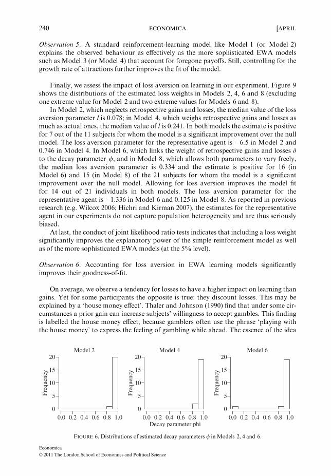
Including retrospective gains and losses slightly decreases the decay parameter.Figure 6 further reveals that the distributions are all unimodal. As expected, most parti-cipants who displayed a significant learning pattern did not discount past experience.This is also reflected in the estimates for the representative agent model that shows a /estimate close to 0.99. The histograms for Models 6 and 7 (cf. Figures 6 and 7) revealthat tying the weight of retrospective gains and losses d to the decay parameter /(Model 6) has a small positive effect on the latter, as the mean values of / are 0.943 inModels 6 and 8 and 0.904 in Model 7.

This leads us to the question of whether tying d to / is a legitimate simplification forour data. The left panel of Figure 7 shows the (joint) distribution of the estimates for dand / in Model 7. Most observations lie in the upper right corner of the joint distributiongraph, confirming the intuition that the parameters should be linked closely. There are,however, some exceptions. Appropriate likelihood ratio tests show that d = / has to berejected for only 6 (5) of the 21 individuals at the 5% (1%) level. The largest differencefor which d = / cannot be rejected is 0.672, whereas the smallest difference that is rejectedis 0.012. The latter is certainly not economically relevant, as two estimates that differ bysuch a small amount are, for all matters of interpretation, equivalent. The clustering of/ and d at 1 is even more pronounced in Model 8, which includes the loss weight l (seeFigure 8). For reasons of parsimony we consider the simplification d = / for our experi-mental data as legitimate. The estimations for the representative agent, however, stronglycontradict this simplification because the estimated coefficients are then d = 0 and/ = 0.99.

Notice that although Model 1 (Model 2) has the same number of freely estimatedparameters as Model 3 (Model 4), it uses less information as it does not take account ofthe bidder’s retrospective gains and losses (d = 0). Surprisingly, however, a pairwise com-parison of the models’ log-likelihoods reveals that the fit of Model 1 (Model 2) is notsubstantially worse than the one of Model 3 (Model 4) (p [ 0.148, according to one-sided t-tests). The EWA models (Models 5–8) introduced by Ho et al. (2007), however,perform considerably better than all other versions of EWA learning in our experiment(p\ 0.001).

Economica



Observation 5. A standard reinforcement-learning model like Model 1 (or Model 2)explains the observed behaviour as effectively as the more sophisticated EWA modelssuch as Model 3 (or Model 4) that account for foregone payoffs. Still, controlling for thegrowth rate of attractions further improves the fit of the model.

Finally, we assess the impact of loss aversion on learning in our experiment. Figure 9shows the distributions of the estimated loss weights in Models 2, 4, 6 and 8 (excludingone extreme value for Model 2 and two extreme values for Models 6 and 8).

In Model 2, which neglects retrospective gains and losses, the median value of the lossaversion parameter l is 0.078; in Model 4, which weighs retrospective gains and losses asmuch as actual ones, the median value of l is 0.241. In both models the estimate is positivefor 7 out of the 11 subjects for whom the model is a significant improvement over the nullmodel. The loss aversion parameter for the representative agent is �6.5 in Model 2 and0.746 in Model 4. In Model 6, which links the weight of retrospective gains and losses dto the decay parameter /, and in Model 8, which allows both parameters to vary freely,the median loss aversion parameter is 0.334 and the estimate is positive for 16 (inModel 6) and 15 (in Model 8) of the 21 subjects for whom the model is a significantimprovement over the null model. Allowing for loss aversion improves the model fitfor 14 out of 21 individuals in both models. The loss aversion parameter for therepresentative agent is �1.336 in Model 6 and 0.125 in Model 8. As reported in previousresearch (e.g. Wilcox 2006; Hichri and Kirman 2007), the estimates for the representativeagent in our experiments do not capture population heterogeneity and are thus seriouslybiased.

At last, the conduct of joint likelihood ratio tests indicates that including a loss weightsignificantly improves the explanatory power of the simple reinforcement model as wellas of the more sophisticated EWAmodels (at the 5% level).

Observation 6. Accounting for loss aversion in EWA learning models significantlyimproves their goodness-of-fit.

On average, we observe a tendency for losses to have a higher impact on learning thangains. Yet for some participants the opposite is true: they discount losses. This may beexplained by a ‘house money effect’. Thaler and Johnson (1990) find that under some cir-cumstances a prior gain can increase subjects’ willingness to accept gambles. This findingis labelled the house money effect, because gamblers often use the phrase ‘playing withthe house money’ to express the feeling of gambling while ahead. The essence of the idea

Model 2

Freq

uenc

y

0.00

5

10

15

20

0.2 0.4 0.6 0.8 1.0

Model 4

Freq

uenc

y

0

5

10

15

20

0.0 0.2 0.4Decay parameter phi

0.6 0.8 1.0

Model 6

Freq

uenc

y

0

5

10

15

20

0.0 0.2 0.4 0.6 0.8 1.0

FIGURE 6. Distributions of estimated decay parameters / in Models 2, 4 and 6.

Economica



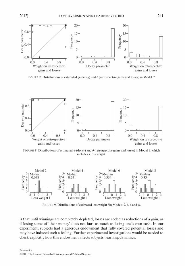
is that until winnings are completely depleted, losses are coded as reductions of a gain, asif losing some of ‘their money’ does not hurt as much as losing one’s own cash. In ourexperiment, subjects had a generous endowment that fully covered potential losses andmay have induced such a feeling. Further experimental investigations would be needed tocheck explicitly how this endowment affects subjects’ learning dynamics.

0.0

+

+++ + +++

+

+++

+

+++ +++

0.4Weight on retrospective

gains and lossesDecay parameter

0.8

0.0

0.4

0.0 0.4 0.8

0

5

10

15

20

Freq

uenc

y

Freq

uenc

y

0.0 0.4Weight on retrospective

gains and losses

0.8

0

5

10

15

20D

ecay

par

amet

er 0.8

FIGURE 7. Distributions of estimated / (decay) and d (retrospective gains and losses) in Model 7.

Freq

uenc

y

0

5

10

15

20

0.0Weight on retrospective

gains and losses

0.4 0.8

Freq

uenc

y

0

5

10

15

20

0.0Decay parameter

0.4 0.80.0Weight on retrospective

gains and losses

+

+++ ++++++++++ ++++++

Dec

ay p

aram

eter

0.4 0.8

0.0

0.4

0.8

FIGURE 8. Distributions of estimated / (decay) and d (retrospective gains and losses) in Model 8, which

includes a loss weight.

Model 2

Freq

uenc

y

–2Loss weight l

012345 Median

0.078

–1 0 1 2 3

Freq

uenc

y

012345

Model 4Median0.241

–2Loss weight l–1 0 1 2 3

Freq

uenc

y

012345

Model 6Median0.334


Freq

uenc

y

012345

Model 8Median0.334


FIGURE 9. Distributions of estimated loss weight l in Models 2, 4, 6 and 8.

Economica



Estimation bias and power analysis

As our analysis and conclusions rely on the outcomes of likelihood ratio tests fornested models, we proceed with assessing the power of this test regarding the lossaversion parameter l. Like Salmon (2001), we are also particularly interested in eval-uating a potential estimation bias with a series of Monte Carlo simulations. This isimportant, as Cabrales and Garcia-Fontes (2000) observed that some EWA para-

1000800600400Number of periods

200


200


200 1000800600400Number of periods


200



200



200



200

l = 0.6l = –0.6

l = 1.0l = –1.0

l = 1.4l = –1.4

l = 0.2l = –0.2

0.0

–0.2

–0.4

–0.6

(Est

imat

ed)

valu

e

1

0

–2

–1

–3

–4

(Est

imat

ed)

valu

e

1

0

–2

–1

–3

(Est

imat

ed)

valu

e

1

0

2

–1

3

4

(Est

imat

ed)

valu

e

1

0

2

–1

3

(Est

imat

ed)

valu

e

1.0

0.0

–1.0

2.0

(Est

imat

ed)

valu

e0.6

0.6

0.8

1.0

0.4

0.40.2

0.2

0.0 0.0

(Est

imat

ed)

valu

e

Median25% and 75% Quantile

Mean

true l = –0.2

true l = –1.0

true l = –1.4 true l = 1.4

true l = 1.0

true l = 0.6

true l = 0.2

Pow

er0.6

0.8

1.0

0.4

0.2

0.0

Pow

er

0.6

0.8

1.0

0.4

0.2

0.0

Pow

er

0.6

0.8

1.0

0.4

0.2

0.0

Pow

er


200

1.0

0.0

–1.0

–2.0

(Est

imat

ed)

valu

e true l = –0.6

FIGURE 10. Estimation bias for loss parameter l and power analysis of test for loss aversionH0 : l ¼ 0 versus

H1 : l 6¼ 0.

Economica



meters are likely to be downward biased and often inaccurate if the number of peri-ods is too small.

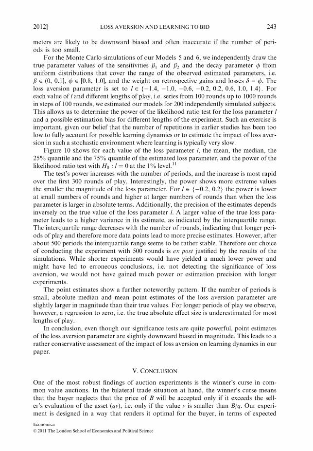
For the Monte Carlo simulations of our Models 5 and 6, we independently draw thetrue parameter values of the sensitivities b1 and b2 and the decay parameter / fromuniform distributions that cover the range of the observed estimated parameters, i.e.b ∈ (0, 0.1], / ∈ [0.8, 1.0], and the weight on retrospective gains and losses d = /. Theloss aversion parameter is set to l ∈ {�1.4, �1.0, �0.6, �0.2, 0.2, 0.6, 1.0, 1.4}. Foreach value of l and different lengths of play, i.e. series from 100 rounds up to 1000 roundsin steps of 100 rounds, we estimated our models for 200 independently simulated subjects.This allows us to determine the power of the likelihood ratio test for the loss parameter land a possible estimation bias for different lengths of the experiment. Such an exercise isimportant, given our belief that the number of repetitions in earlier studies has been toolow to fully account for possible learning dynamics or to estimate the impact of loss aver-sion in such a stochastic environment where learning is typically very slow.

Figure 10 shows for each value of the loss parameter l, the mean, the median, the25% quantile and the 75% quantile of the estimated loss parameter, and the power of thelikelihood ratio test withH0 : l ¼ 0 at the 1% level.11

The test’s power increases with the number of periods, and the increase is most rapidover the first 300 rounds of play. Interestingly, the power shows more extreme valuesthe smaller the magnitude of the loss parameter. For l ∈ {�0.2, 0.2} the power is lowerat small numbers of rounds and higher at larger numbers of rounds than when the lossparameter is larger in absolute terms. Additionally, the precision of the estimates dependsinversely on the true value of the loss parameter l. A larger value of the true loss para-meter leads to a higher variance in its estimate, as indicated by the interquartile range.The interquartile range decreases with the number of rounds, indicating that longer peri-ods of play and therefore more data points lead to more precise estimates. However, afterabout 500 periods the interquartile range seems to be rather stable. Therefore our choiceof conducting the experiment with 500 rounds is ex post justified by the results of thesimulations. While shorter experiments would have yielded a much lower power andmight have led to erroneous conclusions, i.e. not detecting the significance of lossaversion, we would not have gained much power or estimation precision with longerexperiments.

The point estimates show a further noteworthy pattern. If the number of periods issmall, absolute median and mean point estimates of the loss aversion parameter areslightly larger in magnitude than their true values. For longer periods of play we observe,however, a regression to zero, i.e. the true absolute effect size is underestimated for mostlengths of play.

In conclusion, even though our significance tests are quite powerful, point estimatesof the loss aversion parameter are slightly downward biased in magnitude. This leads to arather conservative assessment of the impact of loss aversion on learning dynamics in ourpaper.

V. CONCLUSION

One of the most robust findings of auction experiments is the winner’s curse in com-mon value auctions. In the bilateral trade situation at hand, the winner’s curse meansthat the buyer neglects that the price of B will be accepted only if it exceeds the sell-er’s evaluation of the asset (qv), i.e. only if the value v is smaller than B/q. Our experi-ment is designed in a way that renders it optimal for the buyer, in terms of expected

Economica



revenues, to abstain from bidding B when the seller’s quota (q) is high and to bid Bwith probability 1 when it is low. Consequently, all learning models suggest that ‘win-ners’ should learn to update their profit expectations in the light of experience, andthus should learn to abstain from bidding and to avoid the winner’s curse when theseller’s quota is high.

Although we have provided ample opportunity for learning (250 rounds for eachq-regime), bidding B with a positive probability when the seller’s quota is high remains astrong pattern throughout the experiment and weakens only slightly over time. In ourview, this ex post justifies the relatively large number of rounds of play. Our expectationthat learning in stochastic environments can be rather slow is confirmed at least for thecase when one should abstain from bidding. In contrast, learning to bid B with probabil-ity 1 when the seller’s quota is low was much faster. This is also in line with the size of thefinancial incentives. The expected gain for bidding B when the seller’s quota q is low islarger than the absolute expected loss for bidding B when the seller’s quota is high. Bid-ding B is more profitable for the lower quota than abstaining is for the high one, and istherefore reinforced more strongly. The findings for low and high quotas together seemto show that whether learning is fast or slow depends not on the general environment buton whether one should learn omitting (to bid) or committing (to bid), which, in turn,depends here finally on a numerical parameter, namely the quota of lower evaluation bythe seller.

In general, although we have reduced the bidding task to its simplest expression byremoving confounding effects such as bidders’ strategic interaction, it still seems to bequite a challenge for individuals to learn bidding optimally. We observe considerableindividual heterogeneity of learning dynamics, and there is only a small fraction of peoplewho almost instantaneously converge to optimal bidding. Moreover, learning to avoidthe winner’s curse seems to be rather weak. Either participants understand sooner or laterthat bidding is dangerous when q is high, or never recognize it clearly and are only slightlydiscouraged by (the more frequent) loss experiences.

Important conclusions concerning learning are that (1) loss aversion influences theindividual learning dynamics but is highly heterogeneous, and (2) even though retrospect-ive gains and losses have some influence on learning to bid, their impact seems ratherminor. Finally, we have shown that (3) loss aversion does not seem to be specific to raredecision-making.

APPENDIX

Software screen

Figure A1 displays the decision screen. It features feedback information from the previous round,

the round number, earnings, the prevalent q, the mixed strategy choice, and a calculator symbolthat opens a calculator window.

Instructions (originally in German)

Welcome to the experiment!Please do not speak with other participants from now on.

Economica



Instructions This experiment is designed to study decision-making. You can earn‘real’ money, which will be paid to you in cash at the end of the experiment. The ‘experi-mental currency unit’ will be ‘experimental points (EP)’. EP will be converted to eurosaccording to the exchange rate in the instructions. During the experiment, you and otherparticipants will be asked to take decisions. Your decisions will determine your earningsaccording to the instructions. All participants receive identical instructions. If you haveany questions after reading the instructions, raise your hand. One of the experimenterswill come to you and answer your questions privately. The experiment will last for2 hours maximum.

Roles You are in the role of the buyer; the role of the seller is captured by a robotstrategy of the computer. The computer follows an easy strategy that will be fullydescribed below.

Stages At the beginning of each round you can decide whether you want to ‘bid’ for agood or abstain. For this you can apply a special procedure that we will introduce in amoment. Your bid B is always 25 EP. The value of the good v will be determined inde-pendently and by chance move in every round. v is always between (and including) 0 EPand 100 EP. The chosen values are equally distributed, which means that every integernumber between (and including) 0 EP and 100 EP is the value of the good with equalprobability. The computer as the seller sells the good only when the bid is higher than thevalue multiplied by a factor q.

Mathematically, the computer sells only if B [ qv.The factor q takes on the values 0.4 or 0.6. At the beginning of each round you

will be informed about the value of q in that round. Every 10 rounds, q changes. Keep inmind that you are the only potential buyer of the good. Therefore this is a very specialcase of an auction.

FIGURE A1. Computer screen.

Economica



Special procedure to choose to bid or to abstain The choice between bidding or abstain-ing is made by assigning balls to the two possibilities. You have 10 balls that have to beassigned to the two possibilities. The number of assigned balls corresponds with the prob-ability that a possibility is chosen. Thus each ball corresponds with a probability of 10%.All possible distributions of the 10 balls to the two possibilities are allowed.

Information at the end of each round At the end of each round you receive informationon the value v, whether the good was sold by the computer (or whether the good wouldhave been sold in case you had bid). Additionally, you see your round profit.

Profit

• If you did not bid, your round profit is 0.

• If the bid was smaller than the value of the good multiplied by the factor (B\ qv), the computer

does not sell. No transaction takes place and your round profit is 0.

• If you bid and B[qv, then your round profit depends on the value of the good. In case of a valueof the good that is higher than the bid, v [ B, you make a profit. In case of a value of the good

that is lower than the bid, you make a loss in that round. Losses in single rounds can, of course,be balanced by profits from other rounds.

At the beginning of the experiment you receive an endowment of 1500 EP. At the end of theexperiment, experimental points will be exchanged at a rate of 1 : 200. This means that200EP = 1euro.

Rounds There are 500 rounds in the experiment. In each round you have to take the same decision(assign the balls to the two possibilities of bidding or abstaining) as explained above. Only factor q

will be changed every 10 rounds.

Means of help You will find a calculator on your screen. You are, of course, allowed to write noteson the instruction sheets.

Thank you for participating!

Estimation results

In Table A1, each block of nine lines shows the estimation results for one subject. Line 1 is the null

model. In lines 2–9 follow the different EWA models in the order discussed in the paper: in lines 2and 3 d = 0, in lines 4 and 5 d = 1, in lines 6 and 7 d = /, and in line 9 all parameters are freelyestimated. In the last column of lines 3, 5, 7 and 9 the p-value of the likelihood ratio test with

H0 : l ¼ 0 is reported. In line 8 l = 0 and the p-value of the likelihood ratio test with H0 : d ¼ / isreported in the last column.

TABLE A1ESTIMATION RESULTS FOR EWAMODELS

ID b1 b2 / l dLog-

likelihood

Test v. nullmodel

Pð[v2)

Testfor l or dPð[v2)

1 7.275 �0.012 �778.36\0.001 \0.001 1.000 �778.37 1.0000.002 0.001 1.000 �46.817 �777.96 0.667 0.367

\0.001 \0.001 1.000 �778.37 1.000\0.001 0.092 0.841 �0.857 �777.48 0.414 0.1830.023 0.049 0.001 �772.02 \0.0010.023 0.045 \0.001 0.101 �771.91 0.002 0.6300.023 0.048 \0.001 0.211 �771.87 0.002 0.5740.022 0.033 \0.001 0.913 0.998 �771.25 0.003 0.253

Economica



TABLE A1CONTINUED

ID b1 b2 / l dLog-

likelihood

Test v. nullmodel

Pð[v2)


2 �17.733 53.092 �13.040.009 356.008 1.000 �59.86 1.0000.745 353.519 1.000 �4.036 �21.25 1.000 \0.001

\0.001 168.643 1.000 �13.03 0.9850.025 179.090 1.000 0.459 �14.92 1.000 1.0000.008 2.233 1.000 �36.65 1.0000.517 \0.001 0.804 �1.740 �21.26 1.000 \0.0010.007 3.791 0.993 1.000 �14.09 1.000 \0.0010.617 \0.001 0.830 �1.549 0.100 �8.46 0.027 \0.001

3 7.882 0.069 �1118.74\0.001 0.104 1.000 �1118.34 0.3720.006 0.068 0.252 0.651 �1107.95 \0.001 \0.0010.014 0.021 1.000 �1118.53 0.5230.002 \0.001 1.000 �12.478 �1118.37 0.695 0.572

\0.001 \0.001 1.000 �1118.83 1.000\0.001 \0.001 1.000 13.157 �1118.83 1.000 0.959\0.001 \0.001 1.000 1.000 �1118.83 1.000 0.992\0.001 \0.001 1.000 32.403 1.000 �1118.50 0.922 0.411

4 3.236 4.096 �855.301.502 \0.001 1.000 �857.21 1.0001.063 \0.001 1.000 �0.645 �825.29 \0.001 \0.0011.249 \0.001 0.998 �831.27 \0.0010.925 \0.001 0.992 �0.305 �824.02 \0.001 \0.0010.007 0.032 0.998 �756.61 \0.0010.011 0.029 0.996 0.601 �744.25 \0.001 \0.0010.006 0.058 1.000 0.227 �746.98 \0.001 \0.0010.010 0.037 1.000 0.652 0.177 �738.23 \0.001 0.001

5 6.846 �0.130 �884.02\0.001 \0.001 1.000 �884.35 1.000\0.001 \0.001 1.000 45.511 �884.34 1.000 0.888\0.001 \0.001 1.000 �884.35 1.0000.004 0.007 1.000 25.135 �883.52 0.609 0.200

\0.001 0.001 1.000 �884.27 1.000\0.001 \0.001 1.000 56.855 �883.88 0.869 0.376\0.001 0.001 1.000 1.000 �884.27 1.000 1.000\0.001 \0.001 1.000 65.241 1.000 �883.75 0.910 0.609

6 3.179 1.234 �832.960.161 2.038 1.000 �795.41 \0.001

\0.001 1.404 1.000 0.511 �790.70 \0.001 0.0020.202 1.395 1.000 �798.69 \0.001

\0.001 1.111 1.000 0.632 �789.53 \0.001 \0.0010.001 0.030 1.000 �781.78 \0.001

\0.001 0.019 1.000 0.255 �777.58 \0.001 0.0040.001 0.030 1.000 1.000 �781.78 \0.001 0.991

\0.001 0.019 1.000 0.255 1.000 �777.58 \0.001 0.996

Economica



TABLE A1CONTINUED

ID b1 b2 / l dLog-

likelihood

Test v. nullmodel

Pð[v2)


7 5.600 0.064 �1056.000.049 \0.001 0.908 �1054.33 0.0680.175 \0.001 1.000 2.401 �1051.22 0.008 0.0130.028 \0.001 0.718 �1054.23 0.0600.152 \0.001 1.000 1.539 �1052.82 0.042 0.0930.012 \0.001 0.839 �1053.62 0.0290.010 \0.001 0.900 0.914 �1053.39 0.074 0.4980.012 \0.001 0.824 0.999 �1053.61 0.092 0.8840.011 \0.001 0.898 0.973 1.000 �1053.27 0.141 0.615

8 8.628 0.337 �759.831.029 \0.001 0.992 �679.08 \0.0011.035 \0.001 0.992 0.122 �676.48 \0.001 0.0230.271 \0.001 0.983 �743.59 \0.0010.679 0.129 0.993 0.702 �702.09 \0.001 \0.0010.009 \0.001 1.000 �693.44 \0.0010.044 \0.001 1.000 0.464 �672.25 \0.001 \0.0010.009 \0.001 1.000 1.000 �693.44 \0.001 0.9630.044 \0.001 1.000 0.464 1.000 �672.25 \0.001 0.990

9 63.475 7.556 \0.0014.5e+27 0.102 1.000 \0.001 1.0004.3e+37 0.892 1.000 �3.220 \0.001 1.000 1.0004.5e+27 0.102 1.000 \0.001 1.0004.3e+37 0.892 1.000 �3.220 \0.001 1.000 1.0008.8e+28 0.008 1.000 \0.001 1.0004.0e+54 0.001 0.996 �4.339 \0.001 1.000 1.0008.8e+28 0.008 1.000 1.000 \0.001 1.000 1.0004.0e+54 0.001 0.996 �4.339 0.996 \0.001 1.000 1.000

10 5.895 0.127 �413.330.030 \0.001 1.000 �413.39 1.000

\0.001 \0.001 1.000 129.953 �413.55 1.000 1.0000.015 \0.001 1.000 �413.49 1.000

\0.001 0.002 0.992 20.205 �413.41 1.000 0.6870.001 \0.001 1.000 �410.78 0.024

\0.001 \0.001 1.000 �35.927 �408.33 0.007 0.0270.001 \0.001 1.000 1.000 �410.78 0.078 1.000

\0.001 \0.001 1.000 �48.684 1.000 �407.37 0.008 0.166

11 6.490 3.944 �491.960.813 1.719 0.986 �498.83 1.0000.763 \0.001 0.997 �1.491 �497.10 1.000 0.0630.609 0.847 0.999 �474.69 \0.0010.377 1.236 0.991 0.796 �460.62 \0.001 \0.0010.005 0.019 0.994 �464.03 \0.0010.009 0.015 0.993 0.457 �457.71 \0.001 \0.0010.007 0.027 0.992 0.558 �463.17 \0.001 0.1880.009 0.015 0.993 0.458 1.000 �457.68 \0.001 0.813

Economica



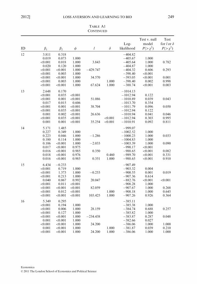
TABLE A1CONTINUED

ID b1 b2 / l dLog-

likelihood

Test v. nullmodel

Pð[v2)


12 3.811 0.318 �404.820.019 0.073 1.000 �405.67 1.000

\0.001 0.018 1.000 3.843 �405.64 1.000 0.7820.020 0.120 1.000 �404.87 1.000

\0.001 \0.001 1.000 �429.747 �404.32 0.606 0.293\0.001 0.003 1.000 �398.40 \0.001\0.001 \0.001 1.000 34.570 �393.05 \0.001 0.001\0.001 0.003 1.000 1.000 �398.40 0.002 0.998\0.001 \0.001 1.000 67.624 1.000 �388.74 \0.001 0.003

13 2.648 0.170 �1014.13\0.001 0.035 \0.001 �1012.94 0.122\0.001 0.001 \0.001 51.086 �1010.89 0.039 0.0430.017 0.015 0.606 �1013.70 0.354

\0.001 0.001 \0.001 38.704 �1011.79 0.096 0.050\0.001 0.035 \0.001 �1012.94 0.1220.001 0.002 \0.001 26.636 �1010.94 0.041 0.046

\0.001 0.035 \0.001 \0.001 �1012.94 0.303 0.9950.001 0.001 \0.001 35.254 \0.001 �1010.91 0.092 0.811

14 5.171 1.485 �999.070.227 0.349 1.000 �1002.52 1.0000.223 0.046 1.000 �1.286 �1000.23 1.000 0.0330.180 0.114 1.000 �1004.83 1.0000.106 \0.001 1.000 �2.033 �1003.39 1.000 0.0900.017 \0.001 0.975 �990.17 \0.0010.016 \0.001 0.985 0.350 �988.65 \0.001 0.0820.018 \0.001 0.976 0.460 �989.70 \0.001 0.3310.016 \0.001 0.985 0.351 1.000 �988.65 \0.001 0.910

15 6.434 �0.233 �907.49\0.001 0.719 1.000 �903.32 0.004\0.001 1.373 1.000 �0.253 �900.55 0.001 0.019\0.001 0.213 1.000 �907.36 0.6140.040 0.067 0.992 20.047 �882.76 \0.001 \0.001

\0.001 0.011 \0.001 �908.28 1.000\0.001 \0.001 \0.001 82.059 �907.67 1.000 0.268\0.001 0.012 \0.001 1.000 �908.18 1.000 0.645\0.001 \0.001 \0.001 103.425 1.000 �907.26 0.926 0.364

16 5.349 0.295 �385.11\0.001 0.194 1.000 �385.38 1.000\0.001 0.006 1.000 28.159 �384.74 0.688 0.257\0.001 0.127 1.000 �385.82 1.000\0.001 \0.001 1.000 �234.438 �383.87 0.287 0.0480.001 \0.001 1.000 �382.66 0.027

\0.001 \0.001 1.000 24.200 �386.06 1.000 1.0000.001 \0.001 1.000 1.000 �381.87 0.039 0.210

\0.001 \0.001 1.000 24.200 1.000 �386.06 1.000 1.000

Economica



TABLE A1CONTINUED

ID b1 b2 / l dLog-

likelihood

Test v. nullmodel

Pð[v2)


17 4.516 �0.130 �970.68\0.001 1.026 0.977 �939.37 \0.0010.148 3.025 0.992 �0.741 �902.03 \0.001 \0.001

\0.001 0.580 0.977 �947.24 \0.0010.055 1.507 0.993 �0.835 �919.52 \0.001 \0.0010.003 \0.001 1.000 �956.84 \0.0010.003 0.018 1.000 �1.664 �837.14 \0.001 \0.0010.003 \0.001 1.000 1.000 �956.84 \0.001 0.9990.003 0.018 1.000 �1.663 1.000 �837.14 \0.001 0.996

18 5.404 �0.767 �897.27\0.001 \0.001 1.000 �908.26 1.000\0.001 0.927 1.000 �0.707 �899.39 1.000 \0.001\0.001 \0.001 1.000 �908.26 1.0000.001 \0.001 1.000 173.948 �901.18 1.000 \0.001

\0.001 \0.001 1.000 �908.26 1.000\0.001 \0.001 1.000 �10.334 �908.26 1.000 0.989\0.001 \0.001 1.000 1.000 �908.26 1.000 0.992\0.001 \0.001 0.999 �18.105 1.000 �887.96 \0.001 \0.001

19 0.624 27.315 �39.840.066 356.131 1.000 �66.88 1.0000.553 354.179 0.999 �6.767 �65.09 1.000 0.0580.659 2.870 1.000 �97.55 1.0000.374 \0.001 1.000 �21.775 �48.06 1.000 \0.0010.654 0.082 1.000 �7.17 \0.0010.776 1.408 1.000 0.812 �7.31 \0.001 1.0000.654 0.082 1.000 1.000 �7.17 \0.001 0.9990.686 0.122 1.000 0.489 1.000 �7.09 \0.001 0.503

20 7.131 3.960 �712.690.529 1.024 1.000 �758.12 1.0000.141 \0.001 1.000 �8.595 �721.49 1.000 \0.0010.468 0.905 0.992 �739.90 1.0000.175 \0.001 1.000 �4.170 �735.15 1.000 0.0020.020 0.019 0.991 �628.46 \0.0010.022 0.017 0.991 0.175 �627.80 \0.001 0.2510.018 0.029 0.993 0.342 �625.83 \0.001 0.0220.019 0.027 0.993 0.047 0.352 �625.80 \0.001 0.046

21 2.638 �0.494 �1153.480.171 \0.001 0.803 �1135.41 \0.0010.172 \0.001 0.815 0.278 �1135.17 \0.001 0.4910.040 0.023 0.749 �1155.39 1.0000.164 0.036 0.834 1.789 �1107.15 \0.001 \0.0010.037 0.006 0.116 �1152.99 0.3200.049 0.016 0.880 1.859 �1104.76 \0.001 \0.0010.064 \0.001 0.793 \0.001 �1139.93 \0.001 \0.0010.051 0.017 0.865 1.793 1.000 �1102.44 \0.001 0.031

Economica



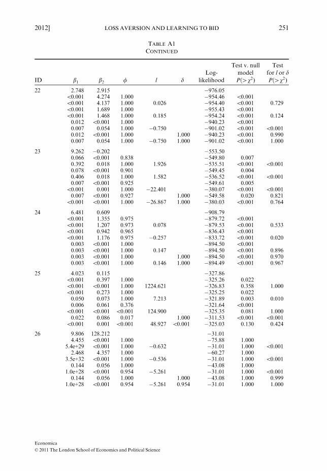
TABLE A1CONTINUED

ID b1 b2 / l dLog-

likelihood

Test v. nullmodel

Pð[v2)


22 2.748 2.915 �976.05\0.001 4.274 1.000 �954.46 \0.001\0.001 4.137 1.000 0.026 �954.40 \0.001 0.729\0.001 1.689 1.000 �955.43 \0.001\0.001 1.468 1.000 0.185 �954.24 \0.001 0.1240.012 \0.001 1.000 �940.23 \0.0010.007 0.054 1.000 �0.750 �901.02 \0.001 \0.0010.012 \0.001 1.000 1.000 �940.23 \0.001 0.9900.007 0.054 1.000 �0.750 1.000 �901.02 \0.001 1.000

23 9.262 �0.202 �553.500.066 \0.001 0.838 �549.80 0.0070.392 0.018 1.000 1.926 �535.51 \0.001 \0.0010.078 \0.001 0.901 �549.45 0.0040.406 0.018 1.000 1.582 �536.52 \0.001 \0.0010.007 \0.001 0.925 �549.61 0.005

\0.001 0.001 1.000 �22.401 �380.07 \0.001 \0.0010.007 \0.001 0.927 1.000 �549.58 0.020 0.821

\0.001 \0.001 1.000 �26.867 1.000 �380.03 \0.001 0.764

24 6.481 0.609 �908.79\0.001 1.355 0.975 �879.72 \0.001\0.001 1.207 0.973 0.078 �879.53 \0.001 0.533\0.001 0.942 0.965 �836.43 \0.001\0.001 1.176 0.975 �0.257 �833.72 \0.001 0.0200.003 \0.001 1.000 �894.50 \0.0010.003 \0.001 1.000 0.147 �894.50 \0.001 0.8960.003 \0.001 1.000 1.000 �894.50 \0.001 0.9700.003 \0.001 1.000 0.146 1.000 �894.49 \0.001 0.967

25 4.023 0.115 �327.86\0.001 0.397 1.000 �325.26 0.022\0.001 \0.001 1.000 1224.621 �326.83 0.358 1.000\0.001 0.273 1.000 �325.25 0.0220.050 0.073 1.000 7.213 �321.89 0.003 0.0100.006 0.061 0.376 �321.64 \0.001

\0.001 \0.001 \0.001 124.900 �325.35 0.081 1.0000.022 0.086 0.017 1.000 �311.53 \0.001 \0.001

\0.001 0.001 \0.001 48.927 \0.001 �325.03 0.130 0.424

26 9.806 128.212 �31.014.455 \0.001 1.000 �75.88 1.000

5.4e+29 \0.001 1.000 �0.632 �31.01 1.000 \0.0012.468 4.357 1.000 �60.27 1.000

3.5e+32 \0.001 1.000 �0.536 �31.01 1.000 \0.0010.144 0.056 1.000 �43.08 1.000

1.0e+28 \0.001 0.954 �5.261 �31.01 1.000 \0.0010.144 0.056 1.000 1.000 �43.08 1.000 0.999

1.0e+28 \0.001 0.954 �5.261 0.954 �31.01 1.000 1.000

Economica



TABLE A1CONTINUED

ID b1 b2 / l dLog-

likelihood

Test v. nullmodel

Pð[v2)


27 63.475 7.556 \0.0018.9e+36 0.612 1.000 \0.001 1.0004.5e+64 1.285 1.000 0.462 \0.001 1.000 1.0008.9e+36 0.612 1.000 \0.001 1.0004.5e+64 1.285 1.000 0.462 \0.001 1.000 1.0005.5e+106 \0.001 1.000 \0.001 1.0002.9e+109 \0.001 1.000 �1.066 \0.001 1.000 1.0005.5e+106 \0.001 1.000 1.000 \0.001 1.000 1.0002.9e+109 \0.001 1.000 �1.066 1.000 \0.001 1.000 1.000

28 15.562 1.402 �33.68\0.001 1.532 1.000 �26.98 \0.001\0.001 1.521 1.000 0.009 �26.98 0.001 0.984\0.001 1.532 1.000 �26.98 \0.001\0.001 1.522 1.000 0.008 �26.98 0.001 0.9890.022 \0.001 \0.001 �34.54 1.000

1206373.459 \0.001 \0.001 �18.946 �32.78 0.406 0.0600.022 \0.001 \0.001 \0.001 �34.54 1.000 0.998

3777953.293 \0.001 \0.001 �17.804 \0.001 �32.78 0.614 1.000

29 5.949 1.389 �921.430.425 \0.001 1.000 �933.07 1.0000.287 \0.001 1.000 �0.718 �920.41 0.363 \0.0010.434 \0.001 1.000 �930.64 1.0000.242 \0.001 0.938 �0.858 �911.78 \0.001 \0.0010.006 \0.001 0.999 �932.58 1.000

\0.001 \0.001 0.998 �22.059 �927.71 1.000 0.0020.008 \0.001 0.996 0.459 �932.01 1.000 0.2850.028 0.030 0.912 �1.311 0.284 �915.62 0.009 \0.001

30 5.081 �0.071 �490.810.026 0.063 0.281 �486.52 0.0030.143 0.256 1.000 �4.992 �475.68 \0.001 \0.0010.028 0.072 0.284 �484.66 \0.0010.065 \0.001 1.000 2.512 �490.15 0.516 1.0000.022 0.048 0.395 �485.51 0.0010.005 0.018 0.977 �1.593 �475.83 \0.001 \0.0010.023 0.053 0.327 1.000 �484.29 0.001 0.1190.008 0.064 0.981 �0.872 \0.001 �464.14 \0.001 \0.001

31 5.949 4.335 �494.490.662 \0.001 1.000 �596.37 1.0000.163 0.042 1.000 �7.671 �501.93 1.000 \0.0010.433 0.303 1.000 �588.14 1.0000.173 0.050 1.000 �6.328 �511.32 1.000 \0.0010.008 0.015 1.000 �439.01 \0.0010.009 0.014 1.000 0.146 �438.59 \0.001 0.3590.008 0.015 1.000 1.000 �439.01 \0.001 1.0000.009 0.014 1.000 0.146 1.000 �438.59 \0.001 1.000

Economica



TABLE A1CONTINUED

ID b1 b2 / l dLog-

likelihood

Test v. nullmodel

Pð[v2)


32 7.061 1.762 �466.980.415 \0.001 0.99 �455.57 \0.0010.531 \0.001 1.000 0.769 �455.43 \0.001 0.5890.241 0.681 0.990 �451.20 \0.0010.298 1.114 0.991 �0.647 �447.71 \0.001 0.0080.010 0.017 0.975 �457.97 \0.0010.010 0.005 0.990 0.920 �454.36 \0.001 0.0070.002 0.020 0.988 1.000 �454.21 \0.001 0.0060.004 0.005 0.995 1.758 1.000 �444.44 \0.001 \0.001

33 11.093 1.191 �384.410.379 0.210 1.000 �390.16 1.0000.033 \0.001 1.000 �12.326 �384.69 1.000 0.0010.275 0.179 1.000 �387.94 1.0000.019 \0.001 1.000 �15.445 �384.97 1.000 0.015

\0.001 \0.001 \0.001 �399.38 1.000\0.001 0.061 \0.001 �1.763 �397.50 1.000 0.052\0.001 \0.001 0.001 0.001 �399.38 1.000 0.999\0.001 0.074 \0.001 �1.493 0.574 �396.47 1.000 0.151

34 3.073 1.920 �905.290.169 0.348 1.000 �917.22 1.0000.088 \0.001 1.000 �12.164 �898.70 0.001 \0.0010.116 0.246 1.000 �917.36 1.0000.007 \0.001 1.000 �74.548 �909.70 1.000 \0.0010.009 \0.001 0.991 �878.00 \0.0010.014 \0.001 1.000 1.150 �871.33 \0.001 \0.0010.013 0.004 0.988 \0.001 �874.16 \0.001 0.0060.012 \0.001 1.000 1.368 0.022 �870.16 \0.001 0.126

35 5.663 1.935 �441.40\0.001 1.201 0.985 �434.55 \0.001\0.001 0.917 0.987 0.288 �434.09 0.001 0.3360.068 0.623 0.984 �441.59 1.0000.045 \0.001 0.912 �13.658 �445.55 1.000 1.0000.006 0.003 0.992 �431.96 \0.0010.003 0.005 0.998 0.584 �432.43 \0.001 1.0000.003 0.006 1.000 \0.001 �425.30 \0.001 \0.0010.003 0.013 1.000 �0.250 \0.001 �425.16 \0.001 \0.001

36 3.653 2.468 �887.440.039 1.601 1.000 �886.44 0.1580.050 4.613 1.000 �0.486 �879.49 \0.001 \0.0010.184 0.692 1.000 �908.45 1.0000.134 \0.001 0.978 �4.269 �874.15 \0.001 \0.0010.011 \0.001 0.986 �903.45 1.0000.007 \0.001 0.956 �4.881 �881.38 0.002 \0.0010.011 \0.001 0.986 1.000 �903.41 1.000 0.7650.011 \0.001 0.949 �3.921 0.284 �879.13 0.001 0.034

Economica



TABLE A1CONTINUED

ID b1 b2 / l dLog-

likelihood

Test v. nullmodel

Pð[v2)


37 4.912 5.346 �160.061.195 \0.001 1.000 �217.91 1.000

\0.001 \0.001 1.000 �4822.192 �382.81 1.000 1.0000.595 0.898 1.000 �195.69 1.0000.850 1.683 1.000 �1.563 �134.06 \0.001 \0.0010.002 0.038 1.000 �85.42 \0.0010.002 0.143 1.000 �0.715 �82.87 \0.001 0.0240.003 0.037 1.000 1.000 �85.00 \0.001 0.3590.002 0.143 1.000 �0.715 1.000 �82.87 \0.001 1.000

38 10.228 �2.658 �420.13\0.001 \0.001 0.296 �478.73 1.000\0.001 \0.001 \0.001 567.432 �478.72 1.000 0.971\0.001 \0.001 0.029 �478.73 1.000\0.001 \0.001 1.000 28.945 �478.73 1.000 1.000\0.001 \0.001 0.619 �478.73 1.000\0.001 \0.001 \0.001 44.321 �478.72 1.000 0.957\0.001 \0.001 \0.001 1.000 �478.72 1.000 0.945\0.001 \0.001 0.034 41.516 \0.001 �478.72 1.000 0.973

39 14.644 41.497 �35.411.6e+30 \0.001 1.000 �35.41 1.0008.3e+36 \0.001 1.000 0.397 �35.41 1.000 0.9943.4e+23 \0.001 1.000 �35.41 1.0009.0e+29 \0.001 1.000 0.368 �35.41 1.000 0.9933.5e+37 \0.001 1.000 �35.41 1.0002.9e+53 \0.001 1.000 �0.955 �35.41 1.000 0.9983.5e+37 \0.001 1.000 1.000 �35.41 1.000 1.0003.9e+58 \0.001 1.000 0.397 1.000 �35.41 1.000 0.995

40 5.645 0.567 �659.270.453 0.077 0.992 �632.88 \0.0010.544 0.140 0.997 �0.087 �633.22 \0.001 1.0000.323 \0.001 0.989 �639.77 \0.0010.445 0.033 0.992 0.241 �635.88 \0.001 0.0050.004 \0.001 1.000 �629.67 \0.0010.007 0.001 1.000 0.334 �627.09 \0.001 0.0230.004 \0.001 1.000 1.000 �629.67 \0.001 0.9790.007 0.001 1.000 0.334 1.000 �627.09 \0.001 0.997

41 7.134 5.115 �337.320.953 1.966 1.000 �359.90 1.0000.577 \0.001 1.000 �2.169 �345.83 1.000 \0.0010.629 2.407 1.000 �334.89 0.0280.171 2.618 1.000 0.399 �333.08 0.014 0.0570.024 0.013 0.985 �364.17 1.0000.043 0.016 0.947 �1.252 �354.19 1.000 \0.0010.024 0.015 0.985 0.849 �364.15 1.000 0.8430.044 0.016 0.946 �1.273 0.876 �354.18 1.000 0.863

Economica



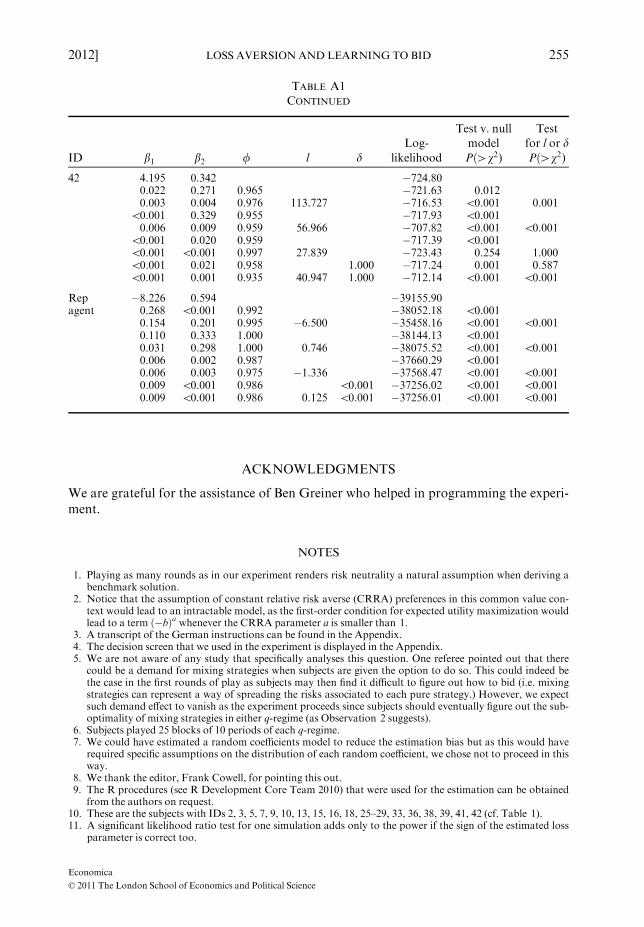
ACKNOWLEDGMENTS

We are grateful for the assistance of Ben Greiner who helped in programming the experi-ment.

NOTES

1. Playing as many rounds as in our experiment renders risk neutrality a natural assumption when deriving abenchmark solution.

2. Notice that the assumption of constant relative risk averse (CRRA) preferences in this common value con-text would lead to an intractable model, as the first-order condition for expected utility maximization wouldlead to a term ð�bÞa whenever the CRRA parameter a is smaller than 1.

3. A transcript of the German instructions can be found in the Appendix.4. The decision screen that we used in the experiment is displayed in the Appendix.5. We are not aware of any study that specifically analyses this question. One referee pointed out that there

could be a demand for mixing strategies when subjects are given the option to do so. This could indeed bethe case in the first rounds of play as subjects may then find it difficult to figure out how to bid (i.e. mixingstrategies can represent a way of spreading the risks associated to each pure strategy.) However, we expectsuch demand effect to vanish as the experiment proceeds since subjects should eventually figure out the sub-optimality of mixing strategies in either q-regime (as Observation 2 suggests).

6. Subjects played 25 blocks of 10 periods of each q-regime.7. We could have estimated a random coefficients model to reduce the estimation bias but as this would have

required specific assumptions on the distribution of each random coefficient, we chose not to proceed in thisway.

8. We thank the editor, Frank Cowell, for pointing this out.9. The R procedures (see R Development Core Team 2010) that were used for the estimation can be obtained

from the authors on request.10. These are the subjects with IDs 2, 3, 5, 7, 9, 10, 13, 15, 16, 18, 25–29, 33, 36, 38, 39, 41, 42 (cf. Table 1).11. A significant likelihood ratio test for one simulation adds only to the power if the sign of the estimated loss

parameter is correct too.

TABLE A1CONTINUED

ID b1 b2 / l dLog-

likelihood

Test v. nullmodel

Pð[v2)


42 4.195 0.342 �724.800.022 0.271 0.965 �721.63 0.0120.003 0.004 0.976 113.727 �716.53 \0.001 0.001

\0.001 0.329 0.955 �717.93 \0.0010.006 0.009 0.959 56.966 �707.82 \0.001 \0.001

\0.001 0.020 0.959 �717.39 \0.001\0.001 \0.001 0.997 27.839 �723.43 0.254 1.000\0.001 0.021 0.958 1.000 �717.24 0.001 0.587\0.001 0.001 0.935 40.947 1.000 �712.14 \0.001 \0.001

Rep �8.226 0.594 �39155.90agent 0.268 \0.001 0.992 �38052.18 \0.001

0.154 0.201 0.995 �6.500 �35458.16 \0.001 \0.0010.110 0.333 1.000 �38144.13 \0.0010.031 0.298 1.000 0.746 �38075.52 \0.001 \0.0010.006 0.002 0.987 �37660.29 \0.0010.006 0.003 0.975 �1.336 �37568.47 \0.001 \0.0010.009 \0.001 0.986 \0.001 �37256.02 \0.001 \0.0010.009 \0.001 0.986 0.125 \0.001 �37256.01 \0.001 \0.001

Economica



REFERENCES

AGRESTI, A. (2010). Analysis of Ordinal Categorical Data. Hoboken: JohnWiley & Sons.

ANDERHUB, V., ENGELMANN, D. and GUTH, W. (2002). An experimental study of the repeated trust game with

incomplete information. Journal of Economic Behavior and Organization, 48, 197–216.ARMANTIER, O. (2004). Does observation influence learning? Games and Economic Behavior, 46, 221–39.BALL, S. B., BAZERMAN, M. H. and CARROLL, J. S. (1991). An evaluation of learning in the bilateral winner’s

curse.Organizational Behavior and Human Decision Processes, 48, 1–22.BAZERMAN, M. H. and SAMUELSON, W. F. (1983). I won the auction but don’t want the prize. Journal of

Conflict Resolution, 27, 618–34.BECKER, G. M., DE GROOT, M. H. and MARSHAK, J. (1964). Measuring utility by a single-response sequential

method. Behavioral Science, 9, 226–32.BENARTZI, S. and THALER, R. H. (1995). Myopic loss aversion and the equity premium puzzle. Quarterly

Journal of Economics, 110, 73–92.BUSH, R. andMOSTELLER, F. (1955). Stochastic Models for Learning. New York: Wiley.

CABRALES, A. and GARCIA-FONTES, W. (2000). Estimating learning models from experimental data. Working

Paper no. 501, Universitat Pompeu Fabra.

CAMERER, C. (2003). Behavioral Game Theory. Princeton, NJ: Princeton University Press.

———— and HO, T.-K. (1999). Experience-weighted attraction (EWA) learning in normal-form games. Econome-

trica, 67, 827–73.CHARNESS, G. and LEVIN, D. (2009). The origin of the winner’s curse: a laboratory study. American Economic

Journal: Microeconomics, 1, 207–36.FISCHBACHER, U. (2007). z-Tree—Zurich toolbox for readymade economic experiments—experimenter’s

manual. Experimental Economics, 10, 171–8.GANDENBERGER, O. (1961).Die Ausschreibung. Heidelberg: Quelle undMeyer.

GARVIN, S. and KAGEL, J. (1994). Learning in common value auctions: some initial observations. Journal of

Economic Organization and Behavior, 25, 351–72.GNEEZY, U. and POTTERS, J. (1997). An experiment on risk taking and evaluation periods. Quarterly Journal of

Economics, 112, 631–45.GUTH, W., IVANOVA-STENZEL, R., KONIGSTEIN, M. and STROBEL, M. (2003). Learning to bid—an exper-

imental study of bid function adjustments in auctions and fair division games. Economic Journal, 103,

477–94.HICHRI, W. and KIRMAN, A. (2007). The emergence of coordination in public good games. European Physical

Journal B, 55(2), 149–59.HO, T.-K., CAMERER, C. and CHONG, J.-K. (2007). Self-tuning experience weighted attraction learning in

games. Journal of Economic Theory, 133, 177–98.————, WANG, X. and CAMERER, C. (2008). Individual differences in EWA learning with partial payoff infor-

mation. Economic Journal, 118, 37–59.JOHNSON, E., GACHTER, S. and HERRMANN, B. (2006). Exploring the nature of loss aversion. CeDEx Discus-

sion Paper no. 2006-02, University of Nottingham.

KAGEL, J. (1995). Auctions: a survey of experimental research. In J. KAGEL and A. ROTH (eds), The Handbook

of Experimental Economics. Cambridge, MA: MIT Press.

KAHNEMAN, D. and TVERSKY, A. (1979). Prospect theory: an analysis of decision under risk. Econometrica, 47,

263–91.NAGEL, R. and TANG, F. (1998). Experimental results on the centipede game in normal form: an investigation

on learning. Journal of Mathematical Psychology, 42, 356–84.OCHS, J. (1995). Games with unique, mixed strategy equilibria: an experimental study. Games and Economic

Behavior, 10, 202–17.OCKENFELS, A. and SELTEN, R. (2005). Impulse balance equilibrium and feedback in first price auctions. Games

and Economic Behavior, 51, 155–70.R DEVELOPMENT CORE TEAM (2010). R: A Language and Environment for Statistical Computing. Vienna:

R Foundation for Statistical Computing.

ROTH, A. E. and EREV, I. (1998). Predicting how people play games: reinforcement learning in experimental

games with unique, mixed strategy equilibria. American Economic Review, 88, 848–80.SALMON, T. (2001). An evaluation of econometric models of adaptive learning. Econometrica, 69, 1597–

628.

SAMUELSON, W. F. and BAZERMAN, M. H. (1985). The winner’s curse in bilateral negotiations. In V. L.SMITH

(ed.), Research in Experimental Economics, Vol. 3. Greenwich: JAI Press, pp. 105–37.

Economica



SELTEN, R. and BUCHTA, J. (1998). Experimental sealed bid first price auctions with directly observed bid func-

tions. In O. D. BUDESCU, I. EREV and R. ZWICK (eds), Games and Human Behavior—Essays in Honor of

Amon Rapoport. Mahwah, NJ: Lawrence Erlbaum.

————, ABBINK, K. and COX, R. (2005). Learning direction theory and the winner’s curse. Experimental Eco-

nomics, 8(1), 5–20.STARMER, C. (2000). Developments in non-expected utility theory: the hunt for a descriptive theory of choice

under risk. Journal of Economic Literature, 38, 332–82.THALER, R. H. and JOHNSON, E. J. (1990). Gambling with the house money and trying to break even: the effects

of prior outcomes on risky choice.Management Science, 36, 643–60.TVERSKY, A. and KAHNEMAN, D. (1992). Advances in prospect theory: cumulative representation of uncer-

tainty. Journal of Risk and Uncertainty, 5, 297–323.VICKREY, W. (1961). Counterspeculation, auctions, and competitive sealed tenders. Journal of Finance, 16,

8–37.WILCOX, N. (2006). Theories of learning in games and heterogeneity bias. Econometrica, 74, 1271–92.

Economica



loss aversion and learning to bid

Documents