LONG TERM FOREIGN CURRENCY EXCHANGE RATEPREDICTIONS

The motivation of this work is to predict foreign currency exchange ratesbetween countries using the long term economic performance of the respectiveeconomies. The predictions are long term - approximately one year in advance- and it is recognised that short term predictions (on a daily basis or shorter)require different approaches to those presented here.

The problem was presented to the Study Group by World Values Ltd. Thiscompany has provided advice for many years on foreign currency exchange ratesusing a model entitled "the currency evaluator", the derivation of which reflectsthe extensive experience of the principals of the company. In brief, points areawarded to each country in respect of its economic performance in eight keyeconomic properties. The points are summed for each country over all the prop-erties, and a comparative ratings or performance table is constructed. Minoradjustments are made if necessary, to this table in the light of practical ex-perience - for example, if a country always scores well with respect to certaineconomic properties, then the effect of those properties might be discountedsomewhat in predictions. The ratings table is then used to make predictions forexchange rates one year ahead. Some details of this process have been publishedby World Values Ltd (1989).

The World Values model is not optimized in the usual mathematical sensein which parameters are determined by fitting predictions to data. Rather, themodel has been tuned according to practical experience. The World Valuesmodel is successful, but has room for improvement. The opinion of the dele-gates at the Study Group was that it was more important for them to suggestalternative mathematically rigorous frameworks for foreign currency predictionsthan to suggest incremental improvements to the World Values model.

The eight key economic properties used by World Values Ltd to make longterm foreign currency exchange rate predictions are described in Section 2. Theseproperties have been identified through years of experience, rather than throughrigorous economic modelling.

Prior to the Study Group, a small amount of computer modelling was un-dertaken in an attempt to improve the World Values forecasts. The resultsof this exercise, incorporating some suggestions made at the Study Group, arepresented in Section 3. Under specific criteria which are described later, thepreliminary results are superior to those achieved by the World Values model.

Our preliminary model possessed some shortcomings from the point of viewof computational efficiency. Accordingly an improved model was suggested atthe Study Group and is described in Section 4. This model is linear and isappropriate when we anticipate that the economic performance of a countryhas a more or less constant effect on the exchange rate. The parameters in themodel are the same for all countries at all times. In our opinion, this linearmodel should be constructed first in any subsequent computer modelling.

In fact, however, it is reasonable to expect that economic performance overtime has a variable effect on exchange rates. That is, stochastic properties shouldbe considered. Accordingly, a more general model incorporating variability wasdeveloped at the Study Group and is described in Section 5. This model is basedon the Kalman filtering approach and would be more elaborate to implementthan the linear model described in Section 4.

The contentious issue of the short term effect versus long term effect of inter-est rates was discussed at the Study Group. These discussions were inconclusive.For completeness, however, we have included a discussion on this topic in Section6. The discussion incorporates a practical suggestion to explore the short termimportance of interest rates.

All models for foreign currency exchange rate prediction rely on a large num-ber of properties and variables. The following notation has been adopted:

m, n refer to countries (m, n = 1, ,8)z refers to time periods (i = 1, , I).

In general, we have used quarterly dataand forecasts.

J refers to economic properties (j = 1, ... , J)

p:nn predicted value of 1 unit of currency min terms of currency n at time ti

P,~m log P~nq:nn actual (market) value of P~nQ~m log q~n

economic property j of country mat time tidimensionless form of e~j

_l_(ei*. _ e .i*)"," mJ J

J

These scaled (dimensionless) properties have the ad'vantage that e~j

e~l % increase p.a. of c.p.i.e~2 % increase p.a. of real money (M3)

e~3 long term interest ratese~4 % increase p.a. of average wagese~5 current account balance as % of GDPe~6 = trade balance as % of importse~7 financial reserves: the number of months

of last months imports that financial reserves will buye:~8 = % increase p.a. of G.N.P.

Further descriptions of these eight properties are given by World ValuesLtd (1989); and \ve note that preliminary smoothing procedures are sometimesapplied before the properties are used in forecasts. For use in Section 6, wedefine

e~9 short term interest rates(e.g. 90 day bank bill).

\Ve also use the concept of 'value' of currencies, but only in a relative sense.Let

For our preliminary model, Wehypothesize that the present value of a cur-rency is related linearly to the eight dimensionless economic properties fourquarters earlier:

8

vi+4 = vi {I + ~ a -ei .}m m ~ J mJj=l

The forecast period of four quarters is the same as in the World Values model.This leads to the predicted exchange rates

In this model, the linearity inherent in the hypothesis (3) has been lost. More-over, there are a number of parameters to be determined, namely eight coef-ficients aj (j = 1, ,8) and seven initial exchange rates P~n(m fixed,n =1, ... , m - 1,m + 1, 8). From these seven initial values, all other initial valuescan be determined using identities (1,2).

Minor modifications were made to the model to predict P~n' rmn and P~n,given initial values P~m' These modifications took the form (for k= 1,2,3)

The choice of weights in the least squares expression (6) should depend on theestimate of P~n rather than qtnn because the presence of observational errorsinside the weights leads to biased estimates and inflated variances. The choiceof qtnn was made out of convenience, bearing in mind the time constraints ofthe IvIISG. In any subsequent investigation, the weights must be carefully cho-sen. The minimization algorithm used was the LMM (Levenberg, Marquadt andMorrison) algorithm for non-linear least squares. In this algorithm, derivativesof P~n with respect to the parameters are required, although these details arenot included here.

To use the preliminary model for predictions, results available at time tf wereused to predict values at t1+4' This procedure was repeated for I = 6, ... ,13.

~

~1987 1968'0 10

0

~

~1987 1988'0 10

N

1988 1988 1988 198920 30 40 1Q

Currency 3 against currency 6

1988 1988 1988 1989 198920 JO 40 1Q 2Q

Currency 3 against currency 7

1988 1988 1988 1988 1989 1989 19891Q 2Q 30 40 1Q 20 30

Currency 2 against currency 6

Figure 1: Illustra.tive one year forecasts of foreign currency exchange rates com-pared with actual values. Legend: 1 - actual exchange rates; 2 - World ValuesLtd forecast; 3 - method of Section 3.

Figure 1 shows sample predictions of the preliminary model compared withactual exchange rates and the predictions of the World Values model. Objective

comparisons between competing models were made using the mean square errors

10 1 12£mn = 8" L.J (Pmn - qmn)

1=10

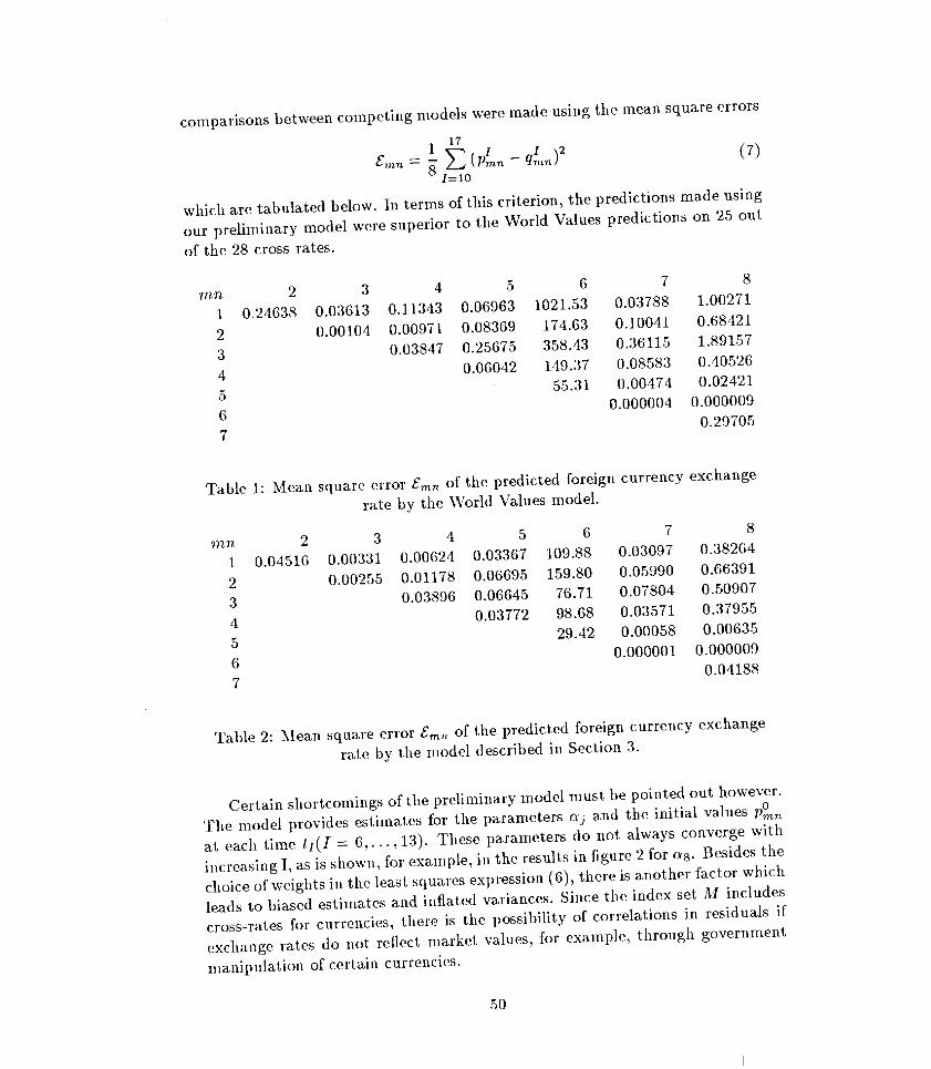
which are tabulated below. In terms of this criterion, the predictions made usingour preliminary model were superior to the World Values predictions on 25 outof the 28 cross rates.

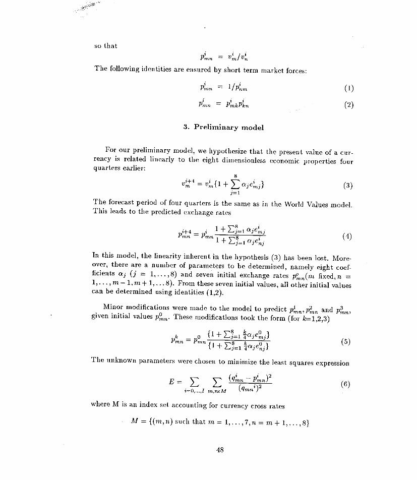
rnn 2 3 4 5 6 7 81 0.24638 0.03613 0.11343 0.06963 1021.53 0.03788 1.002712 0.00104 0.00971 0.08369 174.63 0.10041 0.684213 0.03847 0.25675 358.43 0.36115 1.891574 0.06042 149.37 0.08583 0.405265 55.31 0.00474 0.024216 0.000004 0.0000097 0.29705

Table 1: Mean square error £mn of the predicted foreign currency exchangerate by the World Values model.

rnn 2 3 4 5 6 7 81 0.04516 0.00331 0.00624 0.03367 109.88 0.03097 0.382642 0.00255 0.01178 0.06695 159.80 0.05990 0.663913 0.03896 0.06645 76.71 0.07804 0.509074 0.03772 98.68 0.03571 0.379555 29.42 0.00058 0.006356 0.000001 0.0000097 0.04188

Table 2: Mean square error £mn of the predicted foreign currency exchangerate by the model described in Section 3.

Certain shortcomings of the preliminary model must be pointed out however.The model provides estimates for the parameters aj and the initial values p?nnat each time t 1(I = 6, ... ,13). These parameters do not always converge withincreasing I, as is shown, for example, in the results in figure 2 for a8. Besides thechoice of weights in the least squares expression (6), there is another factor whichleads to biased estimates and inflated variances. Since the index set AI includescross-rates for currencies, there is the possibility of correlations in residuals ifexchange rates do not reflect market values, for example, through governmentmanipulation of certain currencies.

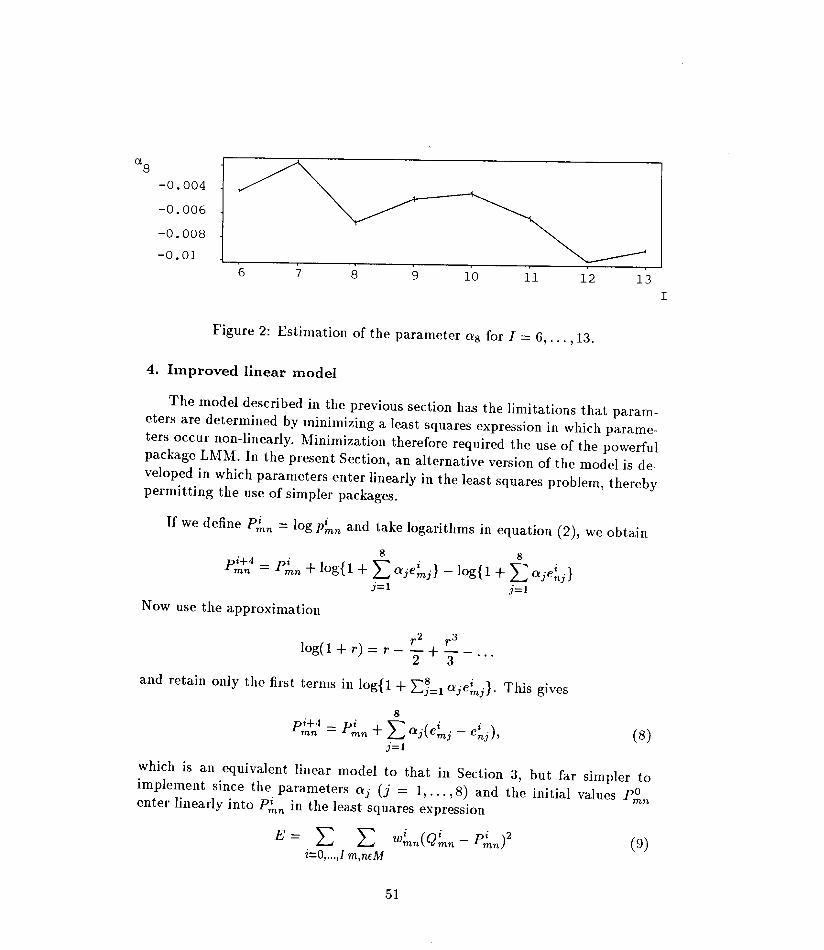
-0.004-0.006-0.008-0.01

The model described in the previous section has the limitations that param-eters are determined by minimizing a least squares expression in which parame-ters occur non-linearly. Minimization therefore required the use of the powerfulpackage LMM. In the present Section, an alternative version of the model is de-veloped in which parameters enter linearly in the least squares problem, therebypermitting the use of simpler packages.

If we define p:nn = log p:nn and take logarithms in equation (2), we obtain

1'2 1'3log(1 + r) = l' - "2 + "3 - ...

and retain only the first terms in log{1 + 2:J=1 Gje:n). This gives

8

Pi+4 _ pi + ""' .( i i )mn - mn L.J GJ emj - enj ,j=1

which is an equivalent linear model to that in Section 3, but far simpler toimplement since the parameters Gj (j = 1, ... ,8) and the initial values P;;menter linearly into p:nn in the least squares expression

E= L

in which Q:nn = logq:nn. (Note that minor modifications as in equation (5) arerequired to predict P~n, P;'n, P;;'n.) Determination of the parameters Qj and theinitial values P;;m requires the solution of a set of simultaneous linear equationsfor which simple standard packages are available.

• Use results available at time tI to predict values at time tI+4 (I6, ... ,13)

• Compare the predictions with those of World Values Ltd and those of thepreliminary model (Section 3)

• Investigate goodness of fit

• Investigate the behaviour of the parameters Qj and P:?m with respect tosign, statistical significance (through the t test), and variability as I isincreased

It would be easier to undertake these investigations with the improved linearmodel than with the preliminary model (Section 3). The improved model willstill lead to biased estimates for the reasons given in Section 3.

If the results of the investigation foreshadowed in the previous section showedthat the parameters in the model appeared to change with time, then this in-dicates that a model which incorporates stochastic variability should be used.Such a model is provided by a Kalman filtering approach (Anderson & Moore,1979).

We start by rewriting equation (8) in the form

8

Pi+4 _ pi + '" i( i i )+ Ximn - mn ~ Qj emj - enj mnj=1

where the parameters Q~ now vary with time and X:nn is assumed to be Gaussianwhite noise with zero mean and variance a;.

In order to use the standard Kalman filtering algorithm, we write for thestate vector,

[pi pi-l pi-2 pi-3 ,i i-I i-2 i-3mn mn mn mn °1 Q1 Q1 Q1

A B1 B2 Bso A 0 0

E'= 0 0 A 0

0 0 0 A

where A is the 4 X 4 matrix

A~[~0 0 1

]0 0 01 0 00 1 0

and ilj is the 4 X 4 matrix

X~n [X:;n30 0 0 ~I-300 0 ~~-30 00... ~~-30 00]

and the ~;-3are Gaussian white noise with mean zero and variance at, so thecovariance matrix Bi of X~n is

02 0 0 0x0 02 0 060 0 02 06

0 0 0 02~8

The observation or measurement equation is

Q~n = IlV/nn + Z:nn

The Kalman filtering algorithm proceeds as follows: start with the initialestimate

[p3 p2 pI pO 3 0mn mn mn mn 0'1 ... 0'1 ...

• •• O'~ ••• O'~]

and the properties a;, a€j' j = 1, ... ,8, a1mn and the covariance matrix R::nn(of V~n). The prediction stage is

which yields V~~lli. The prediction of the observation vector is Q~~li

Q"i+lli = H Vi+1li + E(Zi+lli)mn mn mn·

Then calculate the covariance matrix R~~li (of V~~lli )

This prediction-correction procedure is to be repeated for all m, n in the indexset M.

• This model is in a standard framework, and convergence would be guar-anteed if F had constant coefficients which is, in fact, not the case here

• If the behaviour of the parameters O'~ varies with time, then the Kalmanfiltering approach might give superior performance to the improved linearmodel of Section 4

• Comparisons of forecasts could be made, as before, through the meansquare error crnn

• The performance of the Kalman filtering algorithm depends on a;, a~j'j =1, ... ,8, a2Z • These are "tuning" parameters and need to be chosen care-

mnfully. Literature to guide in the selection of these parameters is available(Anderson & Moore, 1979, Harvey & Peters, 1984) although expert as-sistance would be required by World Values Ltd if this model were to beimplemented

• This model could also be used to investigate sensitivity to variations in theforecast period

• The model developed in this Section does not, however, take account of theconstraints (1,2). To do this, the following straightforward modification ismade. Rewrite equation (12) as

Qi = HVi + Zi

i i i i i iTQ = (Q12"'" Q18, Q23' ... , Q28' ... , Q78)

H = hmn is a 28 X 64 matrix with non-zero entries as follows:

8:S m :S 13: hmn = 1 (n = 5), hmn = -1 (n = 4(m - 7) + 5)

14:S m :S 18: hmn = 1 (n = 9), hmn = -1 (n = 4(m - 13) + 9)

19:5 m:S 22: hmn = 1 (n = 13), hmn = -1 (n = 4(m - 18) + 13)

23 :S m :S 25: hmn = 1 (n = 17), hmn = -1 (n = 4(m - 22) + 17)

26:S m:S 27: hmn = 1 (n = 21), hmn = -1 (n = 4(m - 25) + 21)

m = 28: hmn = 1 (n = 25), hmn = -1 (n = 29)

[ i i-I i-2 i-3 i i-I i-2 i-3VI VI VI VI ... V8 V8 V8 V8i i-I i-2 i-3 i i-I i-2 i-3]T

0'1 0'1 0'1 0'1 .. ·0'8 0'8 0'8 0'8

Zi - [Zi Zi Zi Zi Zi )T- 12' ... , 18' 23"'" 28"'" 78

The covariance matrix of the measurement error vector Zi can be writtenas a2lI lIT if we assume that all the zfnn are Gaussian distributed withzero mean and same variance a2• The modification of equation (11) isagain very straightforward.

• A special case is that o::n does not depend on t. If so, the model requiresless computational effort.

Foreign currency exchange rates are clearly affected in the short term byinterest rate movements. Such short term movements are additional to the longterm effects of interest rates. One approach was to try to identify the short terminterest rate component f in the expression

where p:nn is a predicted exchange rate, q:nn is the market exchange rate, andthe argument of the factor f includes variables that have to be identified. Inan attempt to specify the factor fmn, we examined the 'gain' g:n on investmentsover a period ~:

Here v~ denotes the value of currency 171, and e~9 is the short term interest rateat time ti for country m.

. .. . vi+Cl. vi . vi+Cl.gt _ gt = vt [{(I + et* )~ _ ~} _ {(I + et* )_n_. - I}]

m n n m9 vt t n9 vtn vn n

In this expression, (v:;tCl./v~) and (v~+Cl./ v~) would be predicted by an appro-priate forecasting model, whilst (v:n/v~) = q:nn is the market realization of theexchange rate.

We looked for a general "principle of equilibrium" in which q~n adjustsimmediately to make g~ - g~ = O. If such a principle held, this would providea means for determining the factor fmn described above.

• what forecasting model to choose?

• what method to choose to give e~9? e.g. actual rates at ti, average rates,expected rates, etc.

• how to relate this general principle of equilibrium to definite accountingand economic identities? e.g. the current account must balance

Accordingly, we looked for a simpler approach and now recommend thatthe dimensionless short term interest rate e~9 should be included in the list ofeconomic properties that affect long term foreign currency exchange rates. Minormodifications would be required to incorporate e~9 in the models presented inSections 4 and 5. Standard statistical tests could then be used to decide whetheror not to include e:n9' In particular, the Kalman filtering approach would lenditself well to incorporation of e~9 in the correction (and not prediction) stage.

The preliminary model described in Section 3 yields promising results. Fur-ther development of this preliminary model is possible, but our opinion is thatfurther development would be expedited using the improved linear model de-scribed in Section 4. This follows since the improved linear model has a simplertheoretical framework and would involve less computational work. The Kalmanfiltering model would be more difficult to use than the model of Section 4, butit would be necessary if the parameters O'j exhibited variability with time. Incases where such variability occurs, the Kalman filtering model is optimal.

The models described in this report should have the capability to improvethe foreign currency exchange rate forecasts made by \Vorld Values Ltd.

The moderators for this problem (Noel Barton and Matthew Yiu) would like toacknowledge the support and contributions of Mr James Cowan (vVorld ValuesLtd). The following are also to be thanked for their substantial contributionsto discussions on this problem: Basil Benjamin, Murray Cameron, MargaretGutowski, Joseph Ha, Peter Price, Nancy Spencer and Steve Spencer.

B.D.a. Anderson & J.B. Moore, Optimal Filtering (Prentice-Hall, EnglewoodCliffs, New Jersey, 1979).

A.C. Harvey and S. Peters, "Estimation procedures for structural time-seriesmodels" London School of Economics, Discussion Paper No. 28 (1984).