long-run trends in the concentration of income and wealth daniel waldenström (ifn, stockholm)...

Long-run trends in the Long-run trends in the concentration of income and concentration of income and wealthwealth

Daniel Waldenström (IFN, Stockholm)Daniel Waldenström (IFN, Stockholm)

Presentation at 3rd GLOBALEURONET Summer School, Presentation at 3rd GLOBALEURONET Summer School,

Paris School of Economics, July 10, 2008Paris School of Economics, July 10, 2008

THE ISSUESTHE ISSUES

A.A. What are the What are the long-run cross-country trends long-run cross-country trends in in the concentration of income and wealth? the concentration of income and wealth?

B.B. The role of The role of industrializationindustrialization??

C.C. The role of The role of globalizationglobalization??

D.D. Other determinants?Other determinants?

THIS TALKTHIS TALK

Part I: WealthPart I: Wealth– Long-run trends and revisit impact of industrializationLong-run trends and revisit impact of industrialization– Sample:Sample: 7 countries (old and new data) 7 countries (old and new data)– Time period:Time period: From mid-18th century to present day From mid-18th century to present day

Part II: IncomePart II: Income– Long-run determinants of top income sharesLong-run determinants of top income shares– Role of some economic variablesRole of some economic variables– Sample:Sample: 16 countries 16 countries– Time period:Time period: 1900-2000 1900-2000

Conclusions & some unresolved issuesConclusions & some unresolved issues

Part I: Part I:

The long-run concentration of The long-run concentration of wealth: An overview of recent wealth: An overview of recent

findingsfindings

Outline of Part IOutline of Part I

1.1. Starting pointStarting point

2.2. Wealth concepts and definitionsWealth concepts and definitions

3.3. Country results:Country results: FranceFrance SwitzerlandSwitzerland UKUK USUS DenmarkDenmark NorwayNorway SwedenSweden

4.4. Cross-country comparisonCross-country comparison

5.5. ConclusionsConclusions

1. Starting point1. Starting point

Issues of interest:Issues of interest:

Common vs. specific trendsCommon vs. specific trends

Heterogeneity within the topHeterogeneity within the top

Did wealth inequality increase in the initial phase Did wealth inequality increase in the initial phase of industrialization? (Kuznets hypothesis)of industrialization? (Kuznets hypothesis)

Role of wars, taxes, globalization of the 20th Role of wars, taxes, globalization of the 20th century century

The role of the Scandinavian Welfare State?The role of the Scandinavian Welfare State?

Starting point (2)Starting point (2)

Historical data on wealth inequality:Historical data on wealth inequality:

– FranceFrance, 1807-1994 (Piketty et al, 2006), 1807-1994 (Piketty et al, 2006)– SwitzerlandSwitzerland, 1913-1997 (Dell et al, 2005), 1913-1997 (Dell et al, 2005)– United KingdomUnited Kingdom, 1740-2003 (several authors), 1740-2003 (several authors)– United StatesUnited States, 1774-2002 (several authors), 1774-2002 (several authors)

– DenmarkDenmark, 1789-1996 (various sources), 1789-1996 (various sources)– NorwayNorway, 1789-2002 (various sources), 1789-2002 (various sources)– SwedenSweden, 1800-2006 (various sources), 1800-2006 (various sources)

Variation across these countries:Variation across these countries:– Timing of industrializationTiming of industrialization

– Participation in World WarsParticipation in World Wars

– Level of wealth taxationLevel of wealth taxation

2. Wealth concepts and definitions2. Wealth concepts and definitions

A mix of sources A mix of sources – Estate tax dataEstate tax data– Wealth tax data Wealth tax data – Survey dataSurvey data

Wealth conceptWealth concept– Net worthNet worth = real and financial assets less debts = real and financial assets less debts

– Does (typically) not include: art & jewelry, TV:s etc, Does (typically) not include: art & jewelry, TV:s etc, pension wealth, human capital, public goodspension wealth, human capital, public goods

A mix of observational unitsA mix of observational units– Households (wealth tax-based, survey sources)Households (wealth tax-based, survey sources)– Individuals (deceased, estate-tax based sources)Individuals (deceased, estate-tax based sources)

Concepts (cont’d)Concepts (cont’d)

Computation of top wealth shares:Computation of top wealth shares:– Estimate share of Estimate share of total net worth total net worth that goes to the top 10, 5, that goes to the top 10, 5,

1, 0.1, etc % of 1, 0.1, etc % of all potential wealth holders.all potential wealth holders.

– Reference total wealth: All personal wealth (not only Reference total wealth: All personal wealth (not only taxed wealth) estimated from tax records or national taxed wealth) estimated from tax records or national accountsaccounts

– Reference total for the population: All potential tax units Reference total for the population: All potential tax units (not just those who file tax returns)(not just those who file tax returns)

Problems with tax-based dataProblems with tax-based data– Evasion, avoidance etc.Evasion, avoidance etc.

– Importance grows with systematic differences across Importance grows with systematic differences across distribution and over timedistribution and over time

– We lack compositional information (except for France)We lack compositional information (except for France)

3. French wealth concentration, 1807-3. French wealth concentration, 1807-19941994

0

10

20

30

40

50

60

1800 1840 1880 1920 1960 2000

Share

of

tota

l w

ealt

h (%

)

P99-100

P95-99

P99.9-100

P90-95

Swiss wealth concentration, 1913-Swiss wealth concentration, 1913-19971997

5

10

15

20

25

30

35

40

45

50

1910 1920 1930 1940 1950 1960 1970 1980 1990 2000

Share

of

tota

l w

ealt

h (%

)

P99-100

P95-99

P99.9-100

P90-95

U.K. wealth concentration, 1774-U.K. wealth concentration, 1774-20012001

0

10

20

30

40

50

60

70

80

90

100

1740 1760 1780 1800 1820 1840 1860 1880 1900 1920 1940 1960 1980 2000

Share

of

tota

l w

ealt

h (%

)

P95-100

P99-100

P95-99

England and Wales (1740-1937) U.K. (1938-)

Lindert Lindert (2000)(2000)

Atkinson et Atkinson et alal

IRS IRS (2006)(2006)

10

15

20

25

30

35

40

45

1770 1790 1810 1830 1850 1870 1890 1910 1930 1950 1970 1990

Share

of

tota

l w

ealt

h (%

)

P99-100 (adults)

P99-100 (households)

P90-95 (households)

P95-99 (households)

U.S. wealth concentration, 1774-U.S. wealth concentration, 1774-20012001

Shammas Shammas (1993)(1993)

Lindert Lindert (2000)(2000) Kopzcuk & Saez Kopzcuk & Saez

(2004)(2004)Wolff Wolff (1987, ...)(1987, ...)

Danish wealth concentration, 1789-Danish wealth concentration, 1789-19961996

0

10

20

30

40

50

60

1780 1800 1820 1840 1860 1880 1900 1920 1940 1960 1980 2000

Share

of

tota

l w

ealt

h (%

)

P99-100

P90-95

P95-99

P99.9-100

Norwegian wealth concentration, 1789-Norwegian wealth concentration, 1789-20022002

0

5

10

15

20

25

30

35

40

45

50

1780 1800 1820 1840 1860 1880 1900 1920 1940 1960 1980 2000

Share

of

tota

l w

ealt

h (%

)

P99-100

P95-99

P99.9-100

P90-95

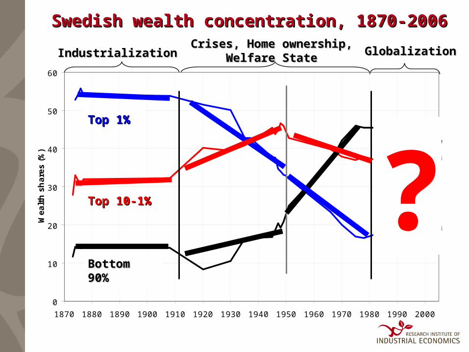
Swedish wealth concentration, 1870-2006Swedish wealth concentration, 1870-2006

0

10

20

30

40

50

60

1870 1880 1890 1900 1910 1920 1930 1940 1950 1960 1970 1980 1990 2000

Wealt

h s

hare

s (%

)

IndustrializationIndustrializationCrises, Home ownership,Crises, Home ownership,

Welfare StateWelfare State GlobalizationGlobalization

?Bottom 90%Bottom 90%

Top 10-1%Top 10-1%

Top 1%Top 1%

What happened in Sweden after What happened in Sweden after 1980?1980?

… … and why does it not show up in the official and why does it not show up in the official statistics?statistics?

Unique Swedish combination of the 1980s & 90s:Unique Swedish combination of the 1980s & 90s:– High taxes on wealth, inheritance and capital incomeHigh taxes on wealth, inheritance and capital income– Financial market boomFinancial market boom– Liberalized capital account (after 1989)Liberalized capital account (after 1989)

Effect: Large fortunes ”disappear”Effect: Large fortunes ”disappear”– Private wealth (and its holders) Private wealth (and its holders) leave Swedenleave Sweden– Capital in Sweden transfered to Capital in Sweden transfered to closely held closely held

companiescompanies

What does this do to the distribution of wealth?What does this do to the distribution of wealth?

Swedish wealth concentration 1950-2005 Swedish wealth concentration 1950-2005 (official series)(official series)

15

20

25

30

35

40

45

50

1950 1960 1970 1980 1990 2000

Förm

ögenhets

andel (%

)

Bottom 90%

Top 1%

Wealt

h s

hare

(%

)W

ealt

h s

hare

(%

)

15

20

25

30

35

40

45

50

1950 1960 1970 1980 1990 2000

Förm

ögenhets

andel (%

)

Swedish wealth concentration 1950-2005 Swedish wealth concentration 1950-2005 (our new series)(our new series)

Bottom 90%

Top 1%

Wealt

h s

hare

(%

)W

ealt

h s

hare

(%

)

How do we estimate the wealth of the How do we estimate the wealth of the rich?rich?

We add fortunes to the wealth of the richest We add fortunes to the wealth of the richest percentile in the domestic populationpercentile in the domestic population

Three additions:Three additions:

1.1. Foreign household wealthForeign household wealth– Net errors and omissions in the Balance of PaymentsNet errors and omissions in the Balance of Payments

– ””Unexplained savings” in the Financial AccountsUnexplained savings” in the Financial Accounts

2.2. Family-firm wealth of rich Swedes in SwedenFamily-firm wealth of rich Swedes in Sweden– Listings of super rich Swedes since 1983Listings of super rich Swedes since 1983

3.3. Wealth of rich Swedes abroadWealth of rich Swedes abroad– Listings of super rich Swedes since 1983Listings of super rich Swedes since 1983

-30%

-20%

-10%

0%

10%

20%

30%

40%

50%

60%

70%

1975 1980 1985 1990 1995 2000 2005

Ack

um

ule

rad r

est

post

som

andel av B

NP

USA

NorwaySweden

Finland

Net errors and omissions (N.E.O.)Net errors and omissions (N.E.O.)A

ccu

mu

late

d n

et

err

ors

an

d o

mis

sio

ns o

ver

Accu

mu

late

d n

et

err

ors

an

d o

mis

sio

ns o

ver

GD

PG

DP

-30%

-20%

-10%

0%

10%

20%

30%

40%

50%

60%

70%

1975 1980 1985 1990 1995 2000 2005

Ack

um

ule

rad r

est

post

som

andel av B

NP

Switzerland

USA

NorwaySweden

Finland

Net errors and omissions (N.E.O.)Net errors and omissions (N.E.O.)A

ccu

mu

late

d n

et

err

ors

an

d o

mis

sio

ns o

ver

Accu

mu

late

d n

et

err

ors

an

d o

mis

sio

ns o

ver

GD

PG

DP

15

20

25

30

35

40

45

1945 1955 1965 1975 1985 1995 2005

Andel av t

ota

lförm

ögenhete

n (%

)Top 1% - Sweden’s official seriesTop 1% - Sweden’s official series

Wealt

h s

hare

(%

)W

ealt

h s

hare

(%

)

SCB official

Effect by adding foreign household wealthEffect by adding foreign household wealthW

ealt

h s

hare

(%

)W

ealt

h s

hare

(%

)

15

20

25

30

35

40

45

1945 1955 1965 1975 1985 1995 2005

Andel av t

ota

lförm

ögenhete

n (%

)

SCB official

+ N.E.O.

Effect by adding family-firm wealth of rich Effect by adding family-firm wealth of rich Swedes living in SwedenSwedes living in Sweden

Wealt

h s

hare

(%

)W

ealt

h s

hare

(%

)

15

20

25

30

35

40

45

1945 1955 1965 1975 1985 1995 2005

Andel av t

ota

lförm

ögenhete

n (%

)

SCB official

+ N.E.O.

+ Rich in Sweden

Effect by adding wealth of rich Swedes Effect by adding wealth of rich Swedes abroadabroad

Wealt

h s

hare

(%

)W

ealt

h s

hare

(%

)

15

20

25

30

35

40

45

1945 1955 1965 1975 1985 1995 2005

Andel av t

ota

lförm

ögenhete

n (%

)

SCB official

+ N.E.O.

+ Rich in Sweden

+ Rich abroad

15

20

25

30

35

40

45

1945 1955 1965 1975 1985 1995 2005

Andel av t

ota

lförm

ögenhete

n (%

)

Comparing Sweden and the U.S. Comparing Sweden and the U.S. (SCF)(SCF)

SCB official

+ N.E.O.

+ Rich in Sweden

+ Rich abroad

USA

+ N.E.O, rich in USA and abroad

Wealt

h s

hare

(%

)W

ealt

h s

hare

(%

)

4. Cross-country P99-100, 1774-4. Cross-country P99-100, 1774-20032003

10

20

30

40

50

60

70

1740 1760 1780 1800 1820 1840 1860 1880 1900 1920 1940 1960 1980 2000

Share

of

tota

l w

ealt

h (%

)

UK*

Denmark

Sweden

France

USA

Switzerland

Norway

Cross-country P95-99, 1774-2003Cross-country P95-99, 1774-2003

15

20

25

30

35

40

45

1740 1760 1780 1800 1820 1840 1860 1880 1900 1920 1940 1960 1980 2000

Share

of

tota

l w

ealt

h (%

)

UK*

Denmark

Sweden

France

USA

Switzerland

Norway

Overview of pre-1914 trendsOverview of pre-1914 trends

Period:Period: ≈≈1780-19141780-1914

Fractile:Fractile: P99-100P99-100 P95-99P95-99

FranceFrance IncreaseIncrease FlatFlat

SwitzerlandSwitzerland -- --

UKUK IncreaseIncrease DecreaseDecrease

USUS IncreaseIncrease Flat?Flat?

DenmarkDenmark DecreaseDecrease FlatFlat

NorwayNorway DecreaseDecrease IncreaseIncrease

SwedenSweden FlatFlat FlatFlat

Overview of long-run trendsOverview of long-run trends

Period:Period: ≈≈1780-19141780-1914 1914-20001914-2000

Fractile:Fractile: P99-100P99-100 P95-99P95-99 P99-100P99-100 P95-99P95-99

FranceFrance IncreaseIncrease FlatFlat DecreaseDecrease FlatFlat

SwitzerlandSwitzerland -- -- FlatFlat FlatFlat

UKUK IncreaseIncrease DecreaseDecrease DecreaseDecrease FlatFlat

USUS IncreaseIncrease Flat?Flat? DecreaseDecrease Flat?Flat?

DenmarkDenmark DecreaseDecrease FlatFlat DecreaseDecrease FlatFlat

NorwayNorway DecreaseDecrease IncreaseIncrease DecreaseDecrease DecreaseDecrease

SwedenSweden FlatFlat FlatFlat DecreaseDecrease DecreaseDecrease

Summarizing Part ISummarizing Part I

Industrialization’s impact on wealth mixedIndustrialization’s impact on wealth mixed

20th century sees massive wealth equalization20th century sees massive wealth equalization– Owner-occupied housingOwner-occupied housing– Wars, crises and progressive taxationWars, crises and progressive taxation– Role of government mixed (public provision of shooling, Role of government mixed (public provision of shooling,

health, pensions, increase inequality of health, pensions, increase inequality of net worthnet worth))

What about the Kuznets inverse-U theory?What about the Kuznets inverse-U theory?– No clear increase in inequality during industrialization, No clear increase in inequality during industrialization,

but a clear decrease thereafterbut a clear decrease thereafter– That is, rather an That is, rather an inverse-inverse-J J curvecurve......

International capital flows may imply that International capital flows may imply that national wealth concentration is underestimatednational wealth concentration is underestimated

Part II: Part II:

The long-run determinants of The long-run determinants of inequality: What can we learn inequality: What can we learn

from top income data?from top income data?

Starting pointStarting point

New database on long-run income inequality: New database on long-run income inequality: – Top income sharesTop income shares

General dissatisfaction with available inequality dataGeneral dissatisfaction with available inequality data– scattered scattered

– short time periodsshort time periods

– different across countries making comparisons difficultdifferent across countries making comparisons difficult

A solution: use A solution: use tax datatax data– available since the early 20th C. available since the early 20th C. Long-run series Long-run series

– available in most countries available in most countries cross-country comparisons cross-country comparisons

– before WWII, primarily top incomes observedbefore WWII, primarily top incomes observed

– focus on the rich important for analyzing driving factorsfocus on the rich important for analyzing driving factors

Income inequality dataIncome inequality data

Top income data: Top income data:

– Main concept: Main concept: gross total income before gross total income before taxes/transferstaxes/transfers

– Tax units: individuals or householdsTax units: individuals or households

– Composition: labor, capital, business income includedComposition: labor, capital, business income included

– Realized capital gains not included*Realized capital gains not included*

Computation of top income shares:Computation of top income shares:– Share of Share of total incometotal income of the top 10, etc % of of the top 10, etc % of all potential all potential

income earners.income earners.

– Reference income not only taxed incomeReference income not only taxed income

– Reference population not just those who file tax Reference population not just those who file tax returnsreturns

FranceFrance

Piketty, 2003, Piketty, 2003, Journal of Political EconomyJournal of Political Economy

United StatesUnited States

Piketty and Saez, 2003, Piketty and Saez, 2003, Quarterly J of Econ.Quarterly J of Econ.

5%

6%

7%

8%

9%

10%

11%

12%

13%

14%

15%

16%

17%

18%

19%

20%

1913 1923 1933 1943 1953 1963 1973 1983 1993 2003

Sh

are

(in

%),

ex

clu

din

g c

apit

al g

ain

s

P90-95 P95-99 P99-100

SwedenSweden

2

6

10

14

18

22

26

30

1900 1920 1940 1960 1980 2000

Shar

e of

inco

me

(%)

P90-95 incl. cap. gains



Roine and Waldenström, 2008, Roine and Waldenström, 2008, J of Public Ec.J of Public Ec.

Other countries...Other countries...

– Canada Canada (Saez and Veall, 2005, (Saez and Veall, 2005, AERAER)) – United kingdom United kingdom (Atkinson, 2005, (Atkinson, 2005, J Roy Stat SocJ Roy Stat Soc))– Switzerland Switzerland & & Germany Germany (Dell, 2005, (Dell, 2005, JEEAJEEA) ) – NetherlandsNetherlands (Atkinson and Salverda 2005, (Atkinson and Salverda 2005, JEEAJEEA))– Australia Australia (Atkinson and Leigh, 2006)(Atkinson and Leigh, 2006)– New Zealand New Zealand (Atkinson and Leigh, 2006, (Atkinson and Leigh, 2006, RevIncWealthRevIncWealth))– IndiaIndia (Banerjee and Piketty, 2005, (Banerjee and Piketty, 2005, WBERWBER))– JapanJapan (Moriguchi and Saez, 2006, (Moriguchi and Saez, 2006, ReStatReStat))– FinlandFinland (Riihilä et al, 2005) (Riihilä et al, 2005)– Spain Spain (Alvaredo and Saez, 2006)(Alvaredo and Saez, 2006)– Argentina Argentina (Alvaredo, 2006)(Alvaredo, 2006)– Ireland Ireland (Nolan, 2007)(Nolan, 2007)– ChinaChina (Piketty and Qian, 2006) (Piketty and Qian, 2006)– Indonesia Indonesia (Leigh and van der Eng, 2006)(Leigh and van der Eng, 2006)– Norway Norway (Aaberge and Atkinson, 2008)(Aaberge and Atkinson, 2008)– Underway: Underway: PortugalPortugal, , DenmarkDenmark, , South AfricaSouth Africa, , African coloniesAfrican colonies

New OUP volumes edited by Atkinson & PikettyNew OUP volumes edited by Atkinson & Piketty

Main findings in top income literatureMain findings in top income literature

Long-run top income trends strikingly similarLong-run top income trends strikingly similar• Up to 1980, income inequality decreasesUp to 1980, income inequality decreases

After 1980, some divergence seem to ariseAfter 1980, some divergence seem to arise• Anglo-Saxon Anglo-Saxon countries experience surge in top sharescountries experience surge in top shares• Continental EuropeanContinental European countries remain on low levels countries remain on low levels

Differences within the top:Differences within the top:• Top precentile has large share of Top precentile has large share of capital incomecapital income• Rest of top decile mainly highly paid Rest of top decile mainly highly paid wage earnerswage earners

Suggested causes (based on country cases):Suggested causes (based on country cases):• Shocks to capital reduces before WWIIShocks to capital reduces before WWII• Progressive taxation holds back increase after WWIIProgressive taxation holds back increase after WWII• After 1980: many candidates...After 1980: many candidates...

This analysisThis analysis

Use new panel with long-term top income shares Use new panel with long-term top income shares

Divide the income distribution into three groups:Divide the income distribution into three groups:– The RichThe Rich (Top 1 percentile) (Top 1 percentile)– The Upper Middle ClassThe Upper Middle Class (Top10–1 percentiles) (Top10–1 percentiles)– The Rest The Rest (Bottom 90 percentiles)(Bottom 90 percentiles)

Try to relate their income shares to other variables:Try to relate their income shares to other variables:– Economic growth, Trade openness, Financial Economic growth, Trade openness, Financial

development, Growth of governmentdevelopment, Growth of government

Allow effects to differ betweenAllow effects to differ between– Levels of economic development (low/medium/high)Levels of economic development (low/medium/high)

– Anglo-Saxon countries and ”rest of the world”Anglo-Saxon countries and ”rest of the world”

– Bank-oriented vs market-oriented financial systemsBank-oriented vs market-oriented financial systems

Potential determinants of inequalityPotential determinants of inequality

Economic growthEconomic growth– Top incomes are more closely tied to the economy Top incomes are more closely tied to the economy

(bonuses, incentive contracts)(bonuses, incentive contracts)

Trade opennessTrade openness– Standard: Capitalists gain in capital abundant countriesStandard: Capitalists gain in capital abundant countries

– ””Superstars” in global labor markets (Rosen, 1980; Superstars” in global labor markets (Rosen, 1980; Gersbach & Schmutzler, 2007)Gersbach & Schmutzler, 2007)

Financial developmentFinancial development– Typically seen as Typically seen as pro-poorpro-poor

• Reduces credit constraints, pools resources (Beck et al. 2007)Reduces credit constraints, pools resources (Beck et al. 2007)

– When is finance When is finance pro-richpro-rich??• When the rich have control over politics and financeWhen the rich have control over politics and finance• At early stages of development (Greenwood & Jovanovic At early stages of development (Greenwood & Jovanovic

1990)1990)

Potential determinants of inequalityPotential determinants of inequality

Marginal income taxationMarginal income taxation– Two potential effects from higher top marginal tax:Two potential effects from higher top marginal tax:

• Lowers pre-tax income through reduced incentives to workLowers pre-tax income through reduced incentives to work

• Raises pre-tax income to compensate for tax increase Raises pre-tax income to compensate for tax increase

AltogetherAltogether: Theory provides conflicting answers: Theory provides conflicting answers

Data (cont’d)Data (cont’d)

Other variables:Other variables:

– GDP/capita GDP/capita and and PopulationPopulation• Source: MaddisonSource: Maddison

– Financial developmentFinancial development: Bank deposits + Stock : Bank deposits + Stock marketmarket• Sources: Mitchell, IFS, FSD, Bordo, Rajan & ZingalesSources: Mitchell, IFS, FSD, Bordo, Rajan & Zingales

– Trade opennessTrade openness: (Exports+Imports)/GDP: (Exports+Imports)/GDP• Sources: Mitchell, López-Córdoba & Meissner, Bordo Sources: Mitchell, López-Córdoba & Meissner, Bordo

– Central government spendingCentral government spending• Sources: Mitchell, Rousseau & Sylla, Bordo, IFS, FSDSources: Mitchell, Rousseau & Sylla, Bordo, IFS, FSD

– Top marginal tax ratesTop marginal tax rates• Sources: Top inc studies, OECD, Rydqvist et al., Bach et al,Sources: Top inc studies, OECD, Rydqvist et al., Bach et al,

First look at the dataFirst look at the data

Several common chocks clearly visibleSeveral common chocks clearly visible

– Great depressionGreat depression

– WWIIWWII

Effects from globalization can be common to the Effects from globalization can be common to the countries in our samplecountries in our sample

– This makes them hard to trace statisticallyThis makes them hard to trace statistically

Top 1% - ”The rich”Top 1% - ”The rich”

0

5

10

15

20

25

30

1900 1910 1920 1930 1940 1950 1960 1970 1980 1990 2000

Tota

l in

com

e s

har

e of

Top1 (%

)

Argentina Australia Canada Finland France GermanyIndia Ireland Japan Netherlands New Zealand SpainSweden Switzerland United Kingdom United States

Top 10-1% - ”The upper middle Top 10-1% - ”The upper middle class”class”

10

15

20

25

30

35

1900 1910 1920 1930 1940 1950 1960 1970 1980 1990 2000

Tota

l in

com

e s

har

e of

Top10-1

(%

)


Variable plotsVariable plots

0.00

0.05

0.10

0.15

0.20

0.25

0.30

0.35

0.40

0.45

0.50

1900 1910 1920 1930 1940 1950 1960 1970 1980 1990 2000

Centr

al govern

ment

spendin

g a

s sh

are

of

GD

P


0

0.5

1

1.5

2

2.5

3

3.5

4

4.5

1900 1910 1920 1930 1940 1950 1960 1970 1980 1990 2000

Tota

l ca

pit

alizati

on a

s sh

are

of

GD

P


0

50

100

150

200

250

300

350

400

1900 1910 1920 1930 1940 1950 1960 1970 1980 1990 2000

Tra

de o

penness

(tr

ade s

hare

in G

DP)


0

5000

10000

15000

20000

25000

30000

1900 1910 1920 1930 1940 1950 1960 1970 1980 1990 2000

GD

P p

er

capit

a (1990 G

-K U

SD)


GDP/capGDP/cap

OpennessOpenness

Total Total capitalizationcapitalization

Gov. Gov. spendingspending

Variable plotsVariable plots

0

10

20

30

40

50

60

70

80

90

100

1900 1910 1920 1930 1940 1950 1960 1970 1980 1990 2000

Top m

arg

inal in

com

e t

ax (%

)


0

10

20

30

40

50

60

70

80

90

100

1900 1910 1920 1930 1940 1950 1960 1970 1980 1990 2000

Top m

arg

inal in

com

e t

ax (%

)

Argentina Australia Canada China Finland FranceGermany India Ireland Japan Netherlands New ZealandSpain Sweden Switzerland United Kingdom United States

Marginal Marginal tax rate tax rate (Preferred)(Preferred)

(rate at inc= (rate at inc= 5xGDP/cap, 5xGDP/cap, statutory)statutory)

Marginal Marginal tax rate 2tax rate 2

(statutory)(statutory)

Econometric methodEconometric method

We model top income shares as being function of:We model top income shares as being function of:– financial development, trade openness, government financial development, trade openness, government

spending, tax progressivity, economic growthspending, tax progressivity, economic growth

Obviously, we cannot claim to establish causality.Obviously, we cannot claim to establish causality.

We use five-year period averages in analysis We use five-year period averages in analysis

The panel dataset is The panel dataset is long and narrowlong and narrow– Fixed effects model (de-meaning) not optimalFixed effects model (de-meaning) not optimal

– Measurement errors likely to be serially correlatedMeasurement errors likely to be serially correlated

Use first-differenced model (Bound & Krueger, 1991)Use first-differenced model (Bound & Krueger, 1991)

Econometric method (2)Econometric method (2)

Error terms also serially correlated. We use two Error terms also serially correlated. We use two approaches to cope with this:approaches to cope with this:

1.1. First-difference GLSFirst-difference GLS (FDGLS - (FDGLS - presented herepresented here))

ΔΔyyitit = = ΔΔXX''ititbb11 + + γγtt + + μμii + + εεit it ((εε ~ AR(1))~ AR(1))

2.2. Dynamic first-differenceDynamic first-difference (DFD - (DFD - inin AppendixAppendix))

ΔΔyyitit = = bb00ΔΔyyit–it–11 + + ΔΔXX''ititbb11 + + γγtt + + μμii + + εεitit

Baseline results (FDGLS)Baseline results (FDGLS)

ΔTop1ΔTop1 ΔTop1ΔTop1 ΔTop10-1ΔTop10-1 ΔTop10-1ΔTop10-1 ΔBot90ΔBot90 ΔBot90ΔBot90

ΔGDPpcΔGDPpc 5.806***5.806*** 6.562***6.562*** ––8.816***8.816*** ––7.017***7.017*** 5.527**5.527** ––1.6541.654

ΔPopΔPop ––4.3624.362 ––12.59**12.59** ––0.5190.519 ––12.0112.01 9.7039.703 22.83*22.83*

ΔOpennessΔOpenness ––8.7998.799 ––2.3122.312 ––0.1990.199 0.3460.346 3.153.15 ––0.3220.322

ΔFindevΔFindev 0.983***0.983*** 1.270***1.270*** 0.1720.172 0.1840.184 ––0.5330.533 ––1.874***1.874***

ΔGovspendΔGovspend 5.9765.976 3.6193.619 ––16.51***16.51*** ––24.05***24.05*** 22.52***22.52*** 23.94***23.94***

ΔMargtax1ΔMargtax1 ––4.390***4.390*** ––3.181**3.181** 10.18***10.18***

ObsObs 126126 9292 9999 7777 9999 7777

Cntry trendsCntry trends YesYes YesYes YesYes YesYes YesYes YesYes

Time effectsTime effects YesYes YesYes YesYes YesYes YesYes YesYes

N countriesN countries 1414 1212 1212 1010 1212 1010

Interacting with Interacting with level of level of developmentdevelopment


ΔGDPpcΔGDPpc 5.437***5.437*** ––8.571***8.571*** 4.896*4.896*

ΔPopΔPop ––4.6904.690 ––5.5845.584 ––2.7022.702 4.234.23 9.6829.682 4.9454.945

ΔGovspendΔGovspend 3.6013.601 5.9415.941 ––18.03***18.03*** ––19.14***19.14*** 24.01***24.01*** 23.50***23.50***

ΔFindevΔFindev 1.045***1.045*** 0.2190.219 ––0.5550.555

ΔOpennessΔOpenness ––9.105***9.105*** ––8.468***8.468*** ––0.2690.269 ––0.7160.716 3.6183.618 3.8313.831

ΔΔGDP×LowGDP×Low 5.067***5.067*** ––9.031***9.031*** 4.534.53

ΔΔGDP×MedGDP×Med 6.406***6.406*** ––7.342***7.342*** 5.9825.982

ΔΔGDP×HighGDP×High 2.6172.617 ––9.841***9.841*** 8.262*8.262*

ΔΔFin×LowFin×Low 1.647*1.647* ––3.263**3.263** 2.0812.081

ΔΔFin×MedFin×Med 0.883*0.883* 0.3340.334 ––1.0151.015

ΔΔFin×HighFin×High 0.862*0.862* 0.4010.401 ––0.8750.875

F: Low=MedF: Low=Med 0.310.31 0.450.45 0.520.52 0.020.02 0.740.74 0.180.18F: Low=HighF: Low=High 0.250.25 0.420.42 0.80.8 0.010.01 0.450.45 0.180.18F: Med=HighF: Med=High 0.070.07 0.980.98 0.340.34 0.940.94 0.590.59 0.90.9ObsObs 126126 126126 9999 9999 9999 9999N countriesN countries 1414 1414 1212 1212 1212 1212

Are Anglo-Saxon countries different?Are Anglo-Saxon countries different?


ΔGDPpcΔGDPpc 5.652***5.652*** 5.537***5.537*** ––9.511***9.511*** ––9.260***9.260*** 7.492**7.492** 6.776**6.776**

ΔPopΔPop ––4.5284.528 ––4.1774.177 ––0.2510.251 1.861.86 8.0868.086 0.3640.364

ΔGovspendΔGovspend 6.0756.075 5.8475.847 ––15.83***15.83*** ––17.07***17.07*** 20.52**20.52** 24.09***24.09***

ΔFinΔFin 0.995***0.995*** 0.982***0.982*** 0.1940.194 0.20.2 ––0.5970.597 ––0.4380.438

ΔOpennessΔOpenness ––8.799***8.799*** ––9.870***9.870*** 0.4720.472 ––1.5081.508 0.9670.967 5.9875.987

ΔGDPΔGDP××ASAS 0.4360.436 2.0362.036 ––6.619*6.619*

ΔOpenΔOpen××ASAS 3.0913.091 6.0336.033 ––16.50***16.50***

ObsObs 126126 126126 9999 9999 9999 9999




The role of financial system?The role of financial system?


ΔGDPpcΔGDPpc 4.606***4.606*** 5.605***5.605*** ––9.221***9.221*** ––8.631***8.631*** 6.132***6.132*** 5.502**5.502**

ΔPopΔPop 1.1661.166 ––4.5534.553 3.4033.403 ––1.0631.063 ––6.9976.997 9.4779.477

ΔGovspendΔGovspend 3.0543.054 4.634.63 ––15.59***15.59*** ––16.21***16.21*** 19.28**19.28** 23.32***23.32***

ΔOpennessΔOpenness ––1.9221.922 ––8.268***8.268*** ––0.3410.341 ––0.2820.282 2.3342.334 3.0613.061

ΔBankdep.ΔBankdep. 2.979***2.979*** 0.2790.279 ––3.367**3.367**

ΔMarketcap.ΔMarketcap. 0.872**0.872** 0.3510.351 ––0.6910.691

ObsObs 168168 128128 129129 101101 129129 101101




Extensions and robustnessExtensions and robustness

We also run analysis on top shares We also run analysis on top shares within within the top. the top. – Top1/Top10 and Top0.1/Top1Top1/Top10 and Top0.1/Top1

– Additional dimension of inequality (e.g., Superstar theory)Additional dimension of inequality (e.g., Superstar theory)

– Removes reference income total (robustness)Removes reference income total (robustness)

– Results are in line with main analysisResults are in line with main analysis

Robustness: Our results are robust to:Robustness: Our results are robust to:

– Restrict analysis to postwar period Restrict analysis to postwar period • Rules out influence from Great DepressionRules out influence from Great Depression

– Dropping Japan from sampleDropping Japan from sample• Japan has no top decile data, hence we have used top 5%.Japan has no top decile data, hence we have used top 5%.

– Replacing Margtax with Margtax2Replacing Margtax with Margtax2• Margtax2 consists of only statutory top rates. More homogenous Margtax2 consists of only statutory top rates. More homogenous

but also more measurement errorbut also more measurement error

Summarizing Part IISummarizing Part II

Analyzing new long-run income inequality panelAnalyzing new long-run income inequality panel

1.1. Finance appears to be strongly pro-richFinance appears to be strongly pro-rich– Bank- and market-based systems alikeBank- and market-based systems alike

2.2. Trade openness: no clear impact on inequalityTrade openness: no clear impact on inequality

3.3. Economic growth is pro-rich while income shares Economic growth is pro-rich while income shares of the upper middle class decreaseof the upper middle class decrease– Extends Dew-Becker & Gordon (2005, 2007)Extends Dew-Becker & Gordon (2005, 2007)

– No support for ”global labor market” for elitesNo support for ”global labor market” for elites

4.4. Government growth accompanies lower Government growth accompanies lower inequalityinequality

CONCLUSION OF TALKCONCLUSION OF TALK

A.A. Trends in Trends in wealth concentrationwealth concentration Up to 1914: Top wealth shares increase in France, US Up to 1914: Top wealth shares increase in France, US

and UK (top 1%). They seem to decrease in Scandinaviaand UK (top 1%). They seem to decrease in Scandinavia

After 1900: Significant equalization in all countries After 1900: Significant equalization in all countries (possibly with reversal after 1980s)(possibly with reversal after 1980s)

Shares of moderately rich (P95-99) fairly stable over Shares of moderately rich (P95-99) fairly stable over timetime

Trends in Trends in income concentrationincome concentration 1900–1980: Top income shares reduced in all countries1900–1980: Top income shares reduced in all countries

1980– : Increased inequality in Anglo-Saxon countries, 1980– : Increased inequality in Anglo-Saxon countries, but still low inequality in Continental Europe, Japan.but still low inequality in Continental Europe, Japan.

Again, shares of upper middle class much more stableAgain, shares of upper middle class much more stable

MAIN CONCLUSIONS (cont’d)MAIN CONCLUSIONS (cont’d)

B.B. Role of industrialization?Role of industrialization? No clear increase in wealth concentration during No clear increase in wealth concentration during

industrialization, but clear decrease thereafterindustrialization, but clear decrease thereafter Suggests Suggests inverse-inverse-JJ rather than Kuznets’ inverse-U curve rather than Kuznets’ inverse-U curve

C.C. Role of globalization?Role of globalization? Trade globalization?? Financial globalization seems to Trade globalization?? Financial globalization seems to

benefit capital owners significantlybenefit capital owners significantly

D.D. Other contributing factors?Other contributing factors? Taxation/growth of governmentTaxation/growth of government hampers top shares hampers top shares House ownershipHouse ownership reduces wealth concentration reduces wealth concentration Economic growthEconomic growth seems to be pro-rich over the long seems to be pro-rich over the long

runrun Financial development Financial development seems to benefit the topseems to benefit the top

Unresolved issues...Unresolved issues...

The rich - who are they?The rich - who are they?– More evidence on professions, industries etc needed More evidence on professions, industries etc needed

Composition of wealth and income?Composition of wealth and income? – Crucial for understanding impact of structural changeCrucial for understanding impact of structural change

Static vs. dynamic inequality?Static vs. dynamic inequality? – Few studies of long-run income and wealth mobilityFew studies of long-run income and wealth mobility– In particular, In particular, intergenerational mobilityintergenerational mobility of interest of interest– Requires high-quality micro-level dataRequires high-quality micro-level data– Kopczuk, Saez & Song on U.S. Kopczuk, Saez & Song on U.S. within carreer within carreer mobilitymobility

Gender issues?Gender issues?– Edlund & Kopzcuk: Men make wealth - women inherit itEdlund & Kopzcuk: Men make wealth - women inherit it

long-run trends in the concentration of income and wealth daniel waldenström (ifn, stockholm)...

Documents

concentration of wealth

wealth concepts

wealth shares

wealth inequality

pension wealth

personal wealth

taxed wealth

danish wealth concentration