long-run marginal electricity generation costs in israel

E L S E V I E R PII:S0301-4215(97)00005-0

Energy Policy, Vol. 25, No. 4, pp. 401-411, 1997 © 1997 Elsevier Science Ltd

Printed in Great Britain. All rights reserved 0301-4215/97 $17.00 + 0.00

Long-run marginal electricity generation costs in Israel

Yigal Porat*, Rotlevi Irith and Ralph Turvey t PO Box 10, Haifa, 31000, Israel

This paper presents two methods for calculating long-run marginal electricity generation costs based on the techniques used for long-term expansion planning. According to the first method, long-run marginal costs are calculated as incremental costs required to supply additional demands-peak, shoulder and off- peak demands, to each hourly demand group separately. These costs include the present value of capital, fuel and operation and maintenance (O&M) costs throughout the planning period. In the second method, the long-run marginal capacity cost element is calculated as an additional/reduced cost resulting from bringing forward/postponing generation capacity investments, in order to supply incremented/ decremented demands in every hour throughout the planning period. The annualized marginal capacity cost is allocated among the hours according to the distribution of the unsupplied energy, and is added to the energy marginal cost to obtain the long-run marginal cost. Both methods are implemented through models used for long-term optimal generation system expansion planning. In addition, the second method uses a chronological simulation of generation system operation. A detailed case study of the Israeli electric generation system is also presented. © 1997 Elsevier Science Ltd. All rights reserved.

Keywords: Long-run marginal cost; Electricity generation costs; Optimal generation expansion planning

Background

The implementation by the Israel Electric Corporation (IEC) of time of day tariffs based on marginal cost calculations, and the need to establish prices for electricity purchased from independent private producers have resulted in renewed interest in the calculation of the marginal cost of electricity. This covers both capacity and energy costs. Electricity tariffs also have to take into account transmission, distribution and administration costs, which do not enter into the calculations of the marginal cost of generation presented here.

This paper presents methods for calculating the long-run marginal cost of electricity, in contrast with methods used to calculate the short-run marginal cost.

The long-run marginal cost of electricity is defined as the expected marginal cost of extra capacity plus the marginal energy production cost (Turvey and Anderson, 1977; Vardi et al, 1977, pp. 270-286; Vardi et al, 1981). Short-run marginal cost does not include capacity costs, but instead substitutes the expected cost of unsupplied energy (Turvey and Ander- son, 1977).

*Corresponding author. *Visiting Professor at the London School of Economics, 30 Sloane Gardens, London SWIW 8DJ, UK

Ideally, for an efficiently expanded welfare-optimal system, the marginal cost of unsupplied energy would equal the long-run marginal cost of supplying that energy. This is the basis for the substitution of the one for the other in models (Zahavi and Feller, 1979; Levin and Zahavi, 1986). In Chapters 1-4 of Turvey (1968) it is noted that, in this equality, the marginal cost of unsupplied energy will exceed the loss of consumer surplus on account of the nuisance and cost of losses of supply which are unanticipated,

For a discussion of the 'optimality' conditions under which the short- and long-run marginal costs would be equal see Crew and Kleindorfer (1986) and Levin and Zahavi (1986). We note that these conditions are rather special; they are not generally satisfied for applied power systems (Anders- son and Bohman, 1985, pp. 279-288) since the expectations held when long-term decisions were taken rarely turn out to have been accurate by the time the decisions have been implemented.

Note that though tariffs are formally a short-term contract; long-term decisions of users are presumably based on an assump- tion that (subject to fuel cost and inflation adjustment) they will last. So they should give a long-term message in order to coordinate the long-term investment decision of consumers with the long-term investffient decisions of the IEC.

The above mentioned models (Zahavi and Feller, 1979;

402 Long-run marginal electricity generation costs in lsrael: Y Porat et al

Levin and Zahavi, 1986) calculate short-run marginal costs. They accept, as input from the user, an arbitrary value of the cost per kWh of unsupplied energy, and multiply this arbitrary value by the hourly loss of load probability. The resulting cost is taken to be the cost of unsupplied energy and is added to the marginal fuel cost to calculate the short-run marginal cost of electricity. It is a major factor entering directly into short-run marginal costs and in determining the relation between marginal costs for peak, shoulder and off-peak hours and for the different seasons of the year.

At present, there is no agreed-upon method of measuring the cost of unsupplied energy directly. Various studies have estimated values from approximately $1.00 kWh -l for all sectors and more than $86.00 kWh -1 for industrial consumers, a range of orders of magnitude (Sanghvi, 1986; Hall et al, 1986; Goett et al, 1988; Woo and Pupp, 1991). Moreover, an estimated system average value for the cost of unsupplied energy does not reflect selective load shedding strategies such as those applied and continuously developed in the Israeli electric system, which are designed to minimize the curtailment costs to the national economy. So the cost of unsupplied energy will be an increasing function of the amount of load that is shed.

The uncertainty concerning the value of short-run marginal costs because of their sensitivity to the cost of unsupplied energy, and the need for tariffs to provide a long-run incen- tive, jointly lead to a need for long-run marginal cost calculations. The two methods presented in this paper answer this need. They reflect the connection of marginal costs to investment costs in capacity expansion, a connection which is absent in short-term marginal costs. As rate makers require time-dependent marginal costs for fixing tariffs for electricity, eliminating the uncertainty entailed in the choice of the cost of unsupplied energy has both practical and theoretical importance.

The system planning approach

The need to base marginal capital cost calculations on investment costs in expansion planning rather than on accounting data is discussed in Wenders (1976, pp. 232-241) and Dick- son and Chamberlin (1984). Two methods are presented in this paper, and both can be viewed as an implementation of the system planning method for calculating marginal costs.

The first method calculates long-run marginal costs as the incremental costs of supplying additional demands to each hourly demand group separately: peak, shoulder and off-peak demands. They include discounted ~ costs of capital, fuel and O&M throughout the planning period. In the second method, incremental capacity cost is calculated as the additional cost incurred to supply incremental demands in each and every hour throughout the planning period. Annu- alized marginal capacity cost is allocated among the hours

according to the distribution of the unsupplied energy and is added to fuel marginal cost to obtain long-run marginal cost.

Marginal cost should be examined in decremental as well as in incremental terms since, with the load forecast being as good as possible, downward and upward deviations from it are equally likely. Since incremental and decremental calculations are similar, however, most of the following discussion explicitly refers to an incremental case.

Both methods are implemented by using EGEAS, a suite of packages for long-term optimal generation system expansion planning developed by Stone and Webster for the Electric Power Research Institute (MIT Energy Laboratory, 1982). In addition, the second method also uses PWEEK, a model for chronological simulation of the generation system operation (P Plus Corporation, 1993), and is thus more complex.

Method 1

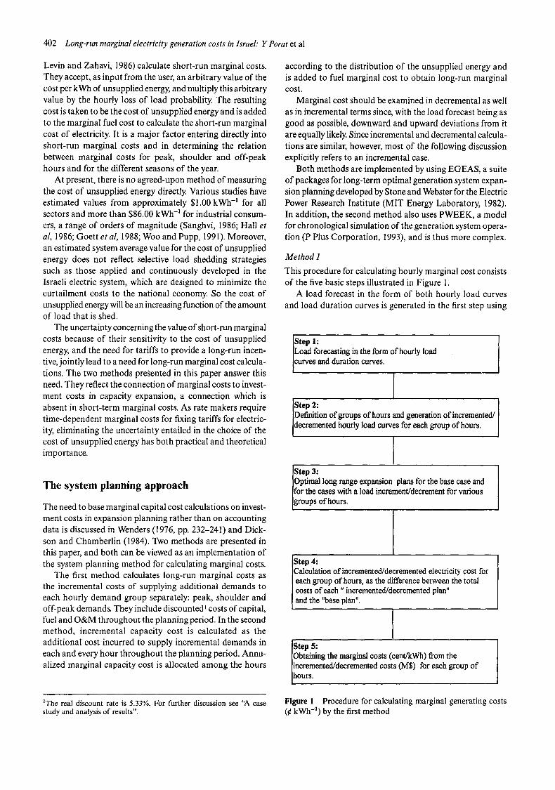
This procedure for calculating hourly marginal cost consists of the five basic steps illustrated in Figure 1.

A load forecast in the form of both hourly load curves and load duration curves is generated in the first step using

I Step 1: Load forecasting in the form of hourly load curves and duration curves.

Definition of groups of hours and generation of incremented/ decremented hourly load curves for each group of hours.

Step 3: ]Optimal long range expansion plans for the base case and [for the cases with aiload increment/decrement for various [groups of hours.

Step 4: Calculation of incremented/decremented electricity cost for each group of hours, as the difference between the total costs of each " incremented/decremented plan" and the "base plan".

I Step 5: Obtaining the marginal costs (cent/kWh) from the incremented/decremented costs (MS) for each group of hours.

~The real discount rate is 5.33%. For further discussion see "A case study and analysis of results".

Figure 1 Procedure for calculating marginal generating costs (¢ kWh -l) by the first method

Long-run marginal electricity generation costs in Israel." Y Porat et al 403

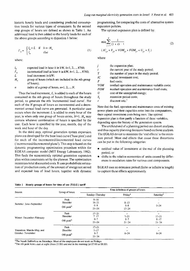
historic hourly loads and considering predicted consump- tion trends for various types of consumers. In the second step groups of hours are defined as shown in Table 1. An additional load is then added to the hourly loads for each of the above groups according to Equation 1 below:

lth

where:

lh + L if h ~ - - H n

I h else (1)

lh l" h

L tt .

expected load in hour h in kW, h=l, 2 ..... 8760; incremented load in hour h in kW, h=l, 2 ..... 8760; load increment in kW; group of hours (which are included in the nth group of hours); index of a group of hours, n=l, 2 ..... N.

Thus the load increment, L, is added to each of the hours contained in the nth group of hours throughout the study period, to generate the nth 'incremented load curve'. For each of the N groups of hours an incremented and a decremented annual load curve are generated. A particular case occurs when the increment L is added to every hour of the year, ie when only one group of hours exists, N=I . Hn may contain whatever combination of hours is specified by the user. Each hour is specified by the year, month, day of the week and hour of the day.

In the third step, optimal generation system expansion plans are developed for the base load curve ('base plan') and for each of the incremented/decremented load curves ('incremented/decremented plans'). This step is based on the dynamic programming optimization procedure within the EGEAS computer model (MIT Energy Laboratory, 1982). This finds the economically optimal generation expansion plan within constraints set by the planner. The optimization minimizes total discounted costs. It uses probabilistic estimation of production costs, of the amount of energy not served and expected loss of load hours, together with dynamic

programming, for comparing the costs of alternative system expansion policies.

The optimal expansion plan is defined by:

T

Z ' mini (1 + r) , - 1 t = l

( ICjj + Fy,t + VOMja + FOMj,t + U),, + S) )

(2)

where:

J t

T IC F VOM FOM U

r

the expansion plan; the current year of the study period; the number of years in the study period; capital investment cost; fuel costs; nonfuel operation and maintenance variable costs; nonfuel operation and maintenance fixed costs; cost of the unsupplied energy; extension period costs; discount rate. J

Note that the fuel, operation and maintenance costs of existing power plants and their capacities enter into the computations, their capital investment costs being zero. The optimal expansion plan is thus partly a function of these variables, depending upon the history of the generation system.

The artificial end of a planning period can distort analyses, and thus capacity planning decisions based on those analyses. The EGEAS device to minimize the 'end effects' is the extension period. Most end effects that cause these distortions can be put in the following categories:

• residual value of investment at the end of the planning period; or

• shifts in the relative economics of units caused by differences in escalation rates for various cost components.

EGEAS uses an extension period (finite or infinite in length) to capture these effects approximately.

Table 1 Hourly groups of hours for time of use (T.O.U.) tariff

Season Group of hours Time definition of groups of hours

Sunday-Thursday Friday ~ Saturday ~

Summer: June-September

Peak 8-16 - - Shoulder 16-21 8-13 -

0-8 0-8 0-24 Off-Peakb 21-24 13-24

Winter: December-February

Peak 17-21 - - Shoulder 7-17 7-21 17-21

Off_peak b 0-7 0-7 0-17 21-24 21-24 21-24

Peak 17-21 Transition:March-May, and Shoulder 7-17

October-November Off_peakb 0-7 21-24

0-24 0-24

~The Israeli Sabbath is on Saturdays. Most of the employees do not work on Fridays. hThe off-peak hours start at night (from 21:00) and end in the morning (at 07:00 or 08:00).

404 Long-run marginal electricity generation costs in Israel." Y Porat et al

2N+ 1 optimal long-term expansion plans are generated: one for the base load curve ('base plan') and another N for each of the incremented load curves ('incremental plan') as well as N additional plans for decremented load curves. In order to eliminate the dependence of the results upon the estimates of the cost of unsupplied energy, each one of the 'incremented/decremented expansion plans' is modified, by altering the size of the postulated load increment/decrement, until the adjusted plan achieves the same present value of unsupplied energy as in the 'base plan'. The results are thus free from the arbitrary nature of estimated costs of unsupplied energy.

The present value of the investment, the fuel costs and the variable and fixed operation and maintenance costs are calculated for the base plan and for all the incremental plans (l~_n<_N). In the fourth step, the incremental cost (as well as decremental cost) for each group of hours is calculated as follows:

MCn= ( IC + F. + VOM, + F O M . ) -

( IC b + F b + VOM b + F O M b ) ($) for each l<n<N (3a)

where:

n index of the 'incremented plan'. The same index is used for the hourly groups in Equation 1, for l<n<N;

MCn incremental marginal cost for the nth 'incremented plan' in $;

ICb, IC,, discounted I investment cost for the 'base plan' and for the nth 'incremented plan', respectively, in $;

Fb, Fn discounted ~ fuel cost for the 'base plan' and for the nth 'incremented plan', respectively, in $;

VOM b, VOM n discounted x variable operation and maintenance costs for the 'base plan' and for the nth 'incremented plan', respectively, in $;

F O M b, FOMn discounted 1 fixed operation and maintenance costs for the base plan' and for the nth 'incremented plan', respectively, in $.

Occasionally, an 'incremental plan' brings forward more efficient generation plants which, at some load levels, displace generation by existing less efficient plants and so result in fuel savings. Incremental capacity cost (MCCn) then includes the additional capital and fixed O&M costs, less any fuel savings (AF) as follows:

M C C n= ( IC~ + F O M , ) - ( IC b + F O M b) -

(AF) ($) for each l<n<N (3b)

present value of the incremented energy over the expansion period for each group of hours (E,,):

MC. m n = ~ or cm n -

M C C n En ($ kWh- l) for each l<n<N

(4)

The decremented case also yields positive marginal costs since both the cost difference and the decremented energy are nega- tive.

The sensitivity of marginal costs to changes in L, the magnitude of the load increment, and to the system reliability criterion 2 should be examined in order to apply this procedure properly. The definition of the groups of hours is embodied in the calculation process and influences it significantly. A different definition of groups of hours would probably yield different marginal costs. 3 Methods for optimal division of the hourly demands into seasonal groups of hours are described in Mosinzon (198 l) and Levin and Zahavi (1986).

M e t h o d 2

This method is built on the principles of the first one. In both, the load change is specified, and the system planners determine the least-cost adjustment of planned capacity addi- tions required to meet the change in load. However, in the second method the specified load change is added for each and every hour over the study period. Marginal capacity cost derives from the expansion generation planning model EGEAS. Its allocation over the hours of the year and the hourly energy cost calculations are based on the chronological simulation model PWEEK. The second method thus treats energy costs in greater detail than the first method, as explained below.

Definition of the groups of hours in this second method, and calculation of the kWh marginal costs, are carried out only at the end of the process. In the first method, on the other hand, the groups of hours are pre-defined in the second step of the procedure.

The procedure in the second method is generally similar to the procedure in the first method, with some exceptions. The procedure described in Figure 1 for the first method, up to the fourth step, is applied for the marginal capacity cost calculation with some adjustments that are clarified below, but the fifth step described in Figure 2 is completely different.

The load forecast in the first step is the same for both methods. In the second step, a load increment of L (MW) is added to each hourly load for the entire study period in order to generate the incremented load curve. It is a particular case of Equation 1 for a single group of hours. In the third

If less efficient power plants, eg an open-cycle gas turbines, with a higher running cost are brought forward, there are no fuel savings and AFequals zero.

Marginal costs per kWh and capacity marginal costs in $ kWh -l (m,,, cm,,, respectively), are obtained in step 5 by dividing the present value of the incremental costs, by the

2The reliability criterion level tbr the generation system planning is an expected loss of 6 load hours per annum, according to the EGEAS model. For further discussion see "A case study and analysis of results". 3The groups of hours in IEC are defined by an analysis of variance of the marginal costs tbr a typical week in each season, ie minimum variance in the groups and maximum variance among the groups (Mosin- zon, 1981). This analysis can also be applied t'or weekly hourly loads.


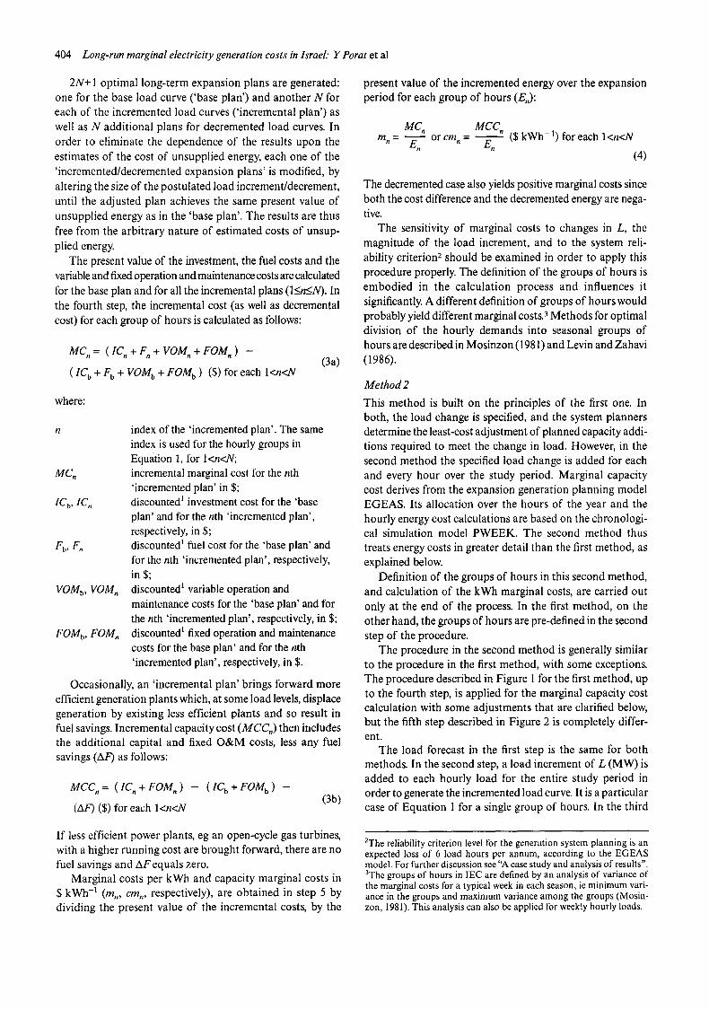
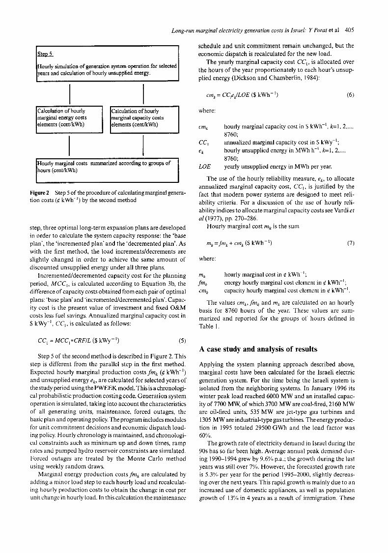
Step 5:

Hourly simulation of generation system operation for selected years and calculation of hourly unsupplied energy.

Calculation of hourly marginal energy costs elements (cent/kWh)

Calculation of hourly marginal capacity costs elements (cent/kWh)

I I Hourly marginal costs summarized according to groups of I hours (cent/kWh) I

Figure 2 Step 5 of the procedure of calculating marginal generation costs (¢ kWh -l) by the second method

step, three optimal long-term expansion plans are developed in order to calculate the system capacity response: the 'base plan', the 'incremented plan' and the 'decremented plan'. As with the first method, the load increments/decrements are slightly changed in order to achieve the same amount of discounted unsupplied energy under all three plans.

Incremented/decremented capacity cost for the planning period, M C C I , is calculated according to Equation 3b, the difference of capacity costs obtained from each pair of optimal plans: 'base plan' and 'incremented/decremented plan'. Capac- ity cost is the present value of investment and fixed O&M costs less fuel savings. Annualized marginal capacity cost in $ kWy -l, CC1, is calculated as follows:

schedule and unit commitment remain unchanged, but the economic dispatch is recalculated for the new load.

The yearly marginal capacity cost CC~, is allocated over the hours of the year proportionately to each hour's unsupplied energy (Dickson and Chamberlin, 1984):

cm k = CCle,/LOE ($ kWh-1) (6)

where:

cm k hourly marginal capacity cost in $ kWh -t, k=l, 2 ..... 8760;

CCI annualized marginal capacity cost in $ kWy-l; ek hourly unsupplied energy in MWh h -l, k=l, 2 .....

8760; LOE yearly unsupplied energy in MWh per year.

The use of the hourly reliability measure, e k, to allocate annualized marginal capacity cost, CC1, is justified by the fact that modern power systems are designed to meet reliability criteria. For a discussion of the use of hourly reliability indices to allocate marginal capacity costs see Vardi et

al (1977), pp. 270-286. Hourly marginal cost mk is the sum

m k = f m k + cm, ($ kWh -1) (7)

where:

m k

c m k

hourly marginal cost in ¢ kWh-~; energy hourly marginal cost element in ¢ kWh-l; capacity hourly marginal cost element in ¢ kWh -I.

The values cm k, f m , and m k are calculated on an hourly basis for 8760 hours of the year. These values are summarized and reported for the groups of hours defined in Table 1.

CC 1 = M C C I *CRF/L ($ kWy-l) (5)

Step 5 of the second method is described in Figure 2. This step is different from the parallel step in the first method. Expected hourly marginal production costs f m k (¢ kWh -1) and unsupplied energy e k, are calculated for selected years of the study period using the PWEEK model. This is a chronological probabilistic production costing code. Generation system operation is simulated, taking into account the characteristics of all generating units, maintenance, forced outages, the basic plan and operating policy. The program includes modules for unit commitment decisions and economic dispatch load- ing policy. Hourly chronology is maintained, and chronological constraints such as minimum up and down times, ramp rates and pumped hydro reservoir constraints are simulated. Forced outages are treated by the Monte Carlo method using weekly random draws.

Marginal energy production costs fmk are calculated by adding a minor load step to each hourly load and recalculat- ing hourly production costs to obtain the change in cost per unit change in hourly load. In this calculation the maintenance

A case study and analysis of results

Applying the system planning approach described above, marginal costs have been calculated for the Israeli electric generation system. For the time being the Israeli system is isolated from the neighboring systems. In January 1996 its winter peak load reached 6000 MW and an installed capacity of 7700 MW, of which 3700 MW are coal-fired, 2160 MW are oil-fired units, 535 MW are jet-type gas turbines and 1305 MW are industrial-type gas turbines. The energy production in 1995 totaled 29500 GWh and the load factor was 60%.

The growth rate of electricity demand in Israel during the 90s has so far been high. Average annual peak demand during 1990-1994 grew by 9.6% p.a.; the growth during the last years was still over 7%. However, the forecasted growth rate is 5.3"/0 per year for the period 1995-2000, slightly decreasing over the next years. This rapid growth is mainly due to an increased use of domestic appliances, as well as population growth of 13% in 4 years as a result of immigration. These

406 Long-run marginal electricity generation costs in Israel: Y Porat et al

resulted in a temporary scarcity of installed generation capacity which was covered by the purchase of an industrial 1105 MW open-cycle gas turbine during the period 1990- 1995.

Using the load forecast for a 20-year period, an optimal generation expansion plan was calculated, beginning in 1995. The alternatives considered included 550 MW coal-fired units, gas turbines (35 MW or 115 MW), a compressed air energy storage plant (300 MW), a pumped storage plant (800 MW) and an oil shale plant (75 MW). Their technical characteristics - capacity, forced outage rates, heat rate curves, maintenance requirements, etc. - were taken from long-term generation expansion planning in the IEC. A real discount rate of 5.33% was used, according to the real capital rate of return on active assets, in order to establish electricity tariffs as recommended by the Committee for the Examination of Electric- ity Tariffs, nominated by the Israeli government (Fogel Committee, 1991). The real capital rate of return, 5.33%, is a weighted capital rate of equity (one-third, 7.5%) and debt (two-thirds, 4.25%).

The reliability criterion for the long-range generating system planning applied in the computations reflects IEC's policy of reaching, after 1995, a reliability level of six expected loss of load hours per annum according to the EGEAS model. This would be optimal with an unsupplied energy cost of 3 $ kWh -l . It requires af~ installed reserve of at least 1150 MW during the whole period of the expansion plan and is expected to be equal to approximately 1.5 unsupplied minutes on average per year per consumer, caused by power cuts due to generation deficiency only (interruption of supply when the demand exceeds the available generation capability). The number of the unsupplied equivalent minutes as a function of the installed generation reserve were estimated using operational data from the IEC for the period 1986-1993 (Kottik et al, 1995). In addition, forced outages of generating units increase the number of unsupplied minutes as a result of under- frequency load shedding. For example, in 1995, a total of 19 unsupplied minutes was partially caused by power cuts (3 min) and partially by under-frequency load shedding (16 min). Various approaches to the determination of reliability criteria for system expansion are discussed in Sanghvi (1986).

The first estimation of the total unsupplied minutes on average per year per consumer made in 1986 was 968 min. They were mostly caused by forced and planned outages in the distribution system. The number of unsupplied minutes was reduced to 502 in 1993 as a result of additional investment resources (50+452 min due to generation and transmission plus distribution). In 1993, the IEC adopted a policy which was aimed at decreasing the total annual unsupplied minutes per consumer to 300 by the year 1996, and to 100 by the year 2000. Most of the IEC resources for improving the reliability of supply were therefore allocated to the distribution system. Nevertheless, it has been also decided to enhance the reliability criterion for the generation expansion planning because of the following reasons: isolation from the neighboring systems with no possible assistance at times of exceptional peak demand and forced outages of generating units; growing dependence of

the national economy on energy supply and the estimated social value of unsupplied energy which is expected to rise in the future from 3 $ kWh -t to 6 and even 9 $ kWh -1.

According to the above-mentioned policy the reliability of supply of the distribution system has been improved by the following: distribution automation including determining the optimal number and location of automation devices, replacing wires and insulators, changing overhead network to underground network, live-line work etc. In 1995, this led to 49+304 unsupplied minutes (generation and transmission plus distribution). More than 70% of the distribution unsupplied minutes were contributed by prearranged interruptions in the distribution system. In the next years a significant cut-down in distribution unsupplied minutes caused by prearranged interruptions is expected, as a result of increasing live-line work. The other 30% are expected to be reduced due to distribution automation and other means.

The following description focuses on an example of the incremental case, the method applying equally to the decremental case. An analysis of various sizes of demand increments and decrements is provided in "Load increment and decrement analysis".

Implementation of the marginal cost calculation

First method. The hourly load curve for the study period was forecast, and a computer model generated the 'incremented load curve' for each of the nine groups of hours, an additional load of 150 MW being added to the original load curve in each hour belonging to that group. Ten optimal expansion plans were then developed for the incremented calculation: the 'base plan' for the original load forecast and one 'incremented plan' for each of the nine groups of hours. Each of these nine 'incremented plans' is based on the relevant 'incremented load curve', and they all have the same accumulated present value of unsupplied energy cost as the 'base plan'. This was achieved by making small changes in the size of the demand increment for each of them.

Incremental cost over the whole study period for each of the nine hourly groups was calculated as the difference between the present value of total costs under the 'incremented plan' and under the 'base plan', with unchanged unsupplied energy. Dividing by the present value of the incremented energy over the whole study period gave the annuitized marginal cost per kWh. An 1 lth optimal expansion plan was developed for incremental load in every hour throughout the study period, for comparison with the results of the second method, whose application was limited to the case of a demand change covering every hour in the year.

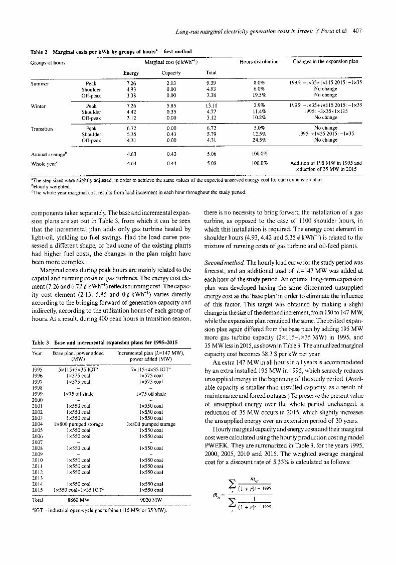
The marginal costs for each 'incremented plan' and the changes in installed capacity during the expansion period are presented in Table 2 for each group of hours. The marginal costs were separated into their energy and capacity elements. The whole- year marginal cost which results from an additional load increment in each hour throughout the study period (5.08 ¢ kWh -~) is similar to the total obtained by summing the marginal costs of each of the nine groups of hours (5.06 ¢ kWh-t).

This similarity also exists for the energy and capacity


Table 2 Marginal costs per kWh by groups of hours a - first method

Groups of hours Marginal cost (¢ kWh -~) Hours distribution Changes in the expansion plan

Energy Capacity Total

Summer Peak 7.26 2.13 9.39 8.0% 1995: -lx35+lx 115 2015:-1x35 Shoulder 4.93 0.00 4.93 6.0% No change Off-peak 3.38 0.00 3.38 19.5% No change

Winter Peak 7.26 5.85 13.11 2.9% 1995: -lx35+lx115 2015:-1x35 Shoulder 4.42 0.35 4.77 11.4% 1995: -3x35+ Ix 115 Off-peak 3.12 0.00 3.12 10.2 % No change

Transition Peak 6.72 0.00 6.72 5.0% No change Shoulder 5.35 0.43 5.79 12.5% 1995:+1x35 2015:-1x35 Off-peak 4.31 0.00 4.31 24.5% No change

Annual average" 4.63 0.43 5.06 100.0%

Whole year ~ 4.64 0.44 5.08 100.0% Addition of 195 MW in 1995 and reduction of 35 MW in 2015

~The step sizes were slightly adjusted, in order to achieve the same values of the expected unserved energy cost for each expansion plan. bHourly weighted. CThe whole year marginal cost results from load increment in each hour throughout the study period.

components taken separately. The base and incremental expansion plans are set out in Table 3, from which it can be seen

that the incremental plan adds only gas turbine heated by

light-oil, yielding no fuel savings. Had the load curve pos-

sessed a different shape, or had some of the existing plants

had higher fuel costs, the changes in the plan might have

been more complex. Marginal costs during peak hours are mainly related to the

capital and running costs of gas turbines. The energy cost ele-

ment (7.26 and 6.72 ¢ kWh -~) reflects running cost. The capacity cost element (2.13, 5.85 and 0¢ kWh -t) varies directly

according to the bringing forward of generation capacity and indirectly, according to the utilization hours of each group of hours. As a result, during 400 peak hours in transition season,

Table 3 Base and incremental expansion plans for 1995-2015

Year Base plan, power added Incremental plan (L=147 MW), (MW) power added (MW)

1995 5xl15+5x35 IGT ~ 7xl15+4x35 IGT" 1996 1x575 coal 1x575 coal 1997 1x575 coal 1x575 coal 1998 - 1999 1x75 oilshale 1x75 oilshale 2000 - 2001 1x550 coal 1x550 coal 2002 1×550 coal 1×550 coal 2003 1x550 coal lx550 coal 2004 lx800 pumped storage lx800 pumped storage 2005 1x550 coal 1x550 coal 2006 1x550 coal 1×550 coal 2007 2008 1x550 coal 1x550 coal 2009 2010 1x550 coal 1x550 coal 2011 1x550 coal lx550 coal 2012 1x550 coal 1x550 coal 2013 - 2014 1x550 coal lx550 coal 2015 1x550 coal+Ix35 IGT a lx550 coal

Total 8860 MW 9020 MW

"IGT - industrial open-cycle gas turbine (115 MW or 35 MW).

there is no necessity to bring forward the installation of a gas

turbine, as opposed to the case of 1100 shoulder hours, in

which this installation is required. The energy cost element in

shoulder hours (4.93, 4.42 and 5.35 ¢ kWh -~) is related to the

mixture of running costs of gas turbine and oil-fired plants.

Secondmethod. The hourly load curve for the study period was

forecast, and an additional load of L= 147 MW was added at

each hour of the study period. An optimal long-term expansion

plan was developed having the same discounted unsupplied

energy cost as the 'base plan' in order to eliminate the influence

of this factor. This target was obtained by making a slight

change in the size of the demand increment, from 150 to 147 MW,

while the expansion plan remained the same. The revised expan-

sion plan again differed from the base plan by adding 195 MW

more gas turbine capacity (2x 115-1x35 MW) in 1995, and

35 MW less in 2015, as shown in Table 3. The annualized marginal

capacity cost becomes 38.3 $ per kW per year.

An extra 147 MW in all hours in all years is accommodated

by an extra installed 195 MW in 1995, which scarcely reduces

unsupplied energy in the beginning of the study period. (Avail-

able capacity is smaller than installed capacity, as a result of

maintenance and forced outages.) To preserve the present value

of unsupplied energy over the whole period unchanged, a

reduction of 35 MW occurs in 2015, which slightly increases

the unsupplied energy over an extension period of 30 years.

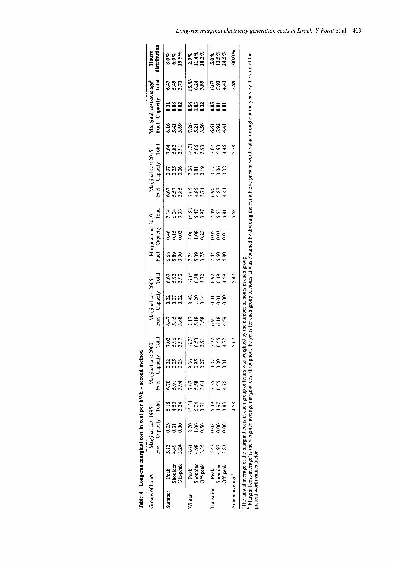
Hourly marginal capacity and energy costs and their marginal

cost were calculated using the hourly production costing model PWEEK. They are summarized in Table 3, for the years 1995,

2000, 2005, 2010 and 2015. The weighted average marginal

cost for a discount rate of 5.33% is calculated as follows:

mnt Z (1 + r)--~k 1995

t

rnn = 1

Z (1 + r)t - 1995 t

408 Long-run marginal electricity generation costs in IsraeL" Y Porat et al

where:

th, weighed marginal cost for the nth group of hours (¢ kWh-~);

m,, marginal cost in year t for the nth group of hours (¢ kWh-~);

r discount rate; t calculation year (1995, 2000, 2010, 2015).

Winter peak marginal costs are the highest because of the high demand-levels during the narrow peak, and winter shoulder marginal costs are almost as high as summer and transition peaks. The summer and transition marginal costs are almost at the same level. This phenomenon is probably a result of intensive plant maintenance during the spring and the autumn (transition) seasons, because of their relatively low loads.

Comparison between the two calculation methods

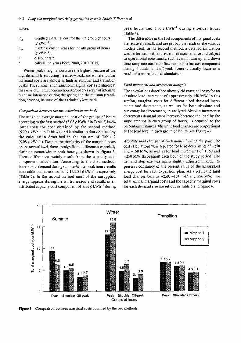
The weighted average marginal cost of the groups of hours according to the first method (5.06 ¢ kWh -~ in Table 2) is 4% lower than the cost obtained by the second method (5.29 ¢ kWh -~ in Table 4), and is similar to that obtained by the calculation described in the bot tom of Table 2 (5.08 ¢ kWh-~). Despite the similarity of the marginal costs on the annual level, there are significant differences, especially during summer/winter peak hours, as shown in Figure 3. These differences mainly result from the capacity cost component calculation. According to the first method, incremental demand during summer/winter peak hours results in an additional investment of 2.13/5.85 ¢ kWh -~, respectively (Table 2). In the second method most of the unsupplied energy appears during the winter season and results in an attributed capacity cost component of 8.56 ¢ kWh -~ during

peak hours and 1.03 ¢ kWh -1 during shoulder hours (Table 4).

The differences in the fuel components of marginal costs are relatively small, and are probably a result of the various models used. In the second method, a detailed simulation was performed, with more detailed maintenance and subject to operational constraints, such as minimum up and down time, ramp rate, etc. In the first method the fuel cost component during shoulder and off-peak hours is usually lower as a result of a more detailed simulation.

Load increment and decrement analysis

The calculations described above yield marginal costs for an absolute load increment of approximately 150 MW In this section, marginal costs for different sized demand increments and decrements, as well as for both absolute and percentage load increments, are analyzed. Absolute increments/ decrements demand steps increase/decrease the load by the same amount in each group of hours, as opposed to the percentage instances, where the load changes are proportional to the load level in each group of hours (see Figure 4).

Absolute load changes of each hourly load of the year The cost calculations were repeated for load decrements of -250 and -150 MW, as well as for load increments of +150 and +250 MW throughout each hour of the study period. The demand step size was again slightly adjusted in order to preserve constancy of the present value of the unsupplied energy cost for each expansion plan. As a result the final load changes became -250, -164, 147 and 256 MW The total annual marginal costs and the capacity marginal costs for each demand size are set out in Table 5 and figure 4.

20

~" 15

oo

._=

0~

E

I-

10

i

Summer

9.4

5.5

@ Peak

5.5

Shoulder Off-peak

Winter Transition

15.8

15,'

6.76.7 6.2

ii ''j, li Peak Shoulder Off-peak Peak

Groups of hours

/ ml Method 1 |

J Method 2

5,85.9

Shoulder Off-peak

Figure 3 Comparison between marginal costs obtained by the two methods

Long-run marginal electricity generation costs in Israel. • Y Porat et al 409

8

I

.=.

8

.~.

¢1

e ,

o ¢'4

o

"N "

0

o

£

• o °

0 0 o

m q q [ ~

I I

~ ~o

e .

~ ~'"

~ d d d d d

2 ~ d

E

e~

0 e -

e -

e -

e~

E

e~

3.=

. M

~ a

- a ~ o o

[-

410 Long-run marginal electricity generation costs in Israel." Y Porat et al

Absolute demand step Percentage step

e- ¢D

r" 5

t.8 []

Q-2

0 L)

1 L#

0

-250

6

marginal cost 5.1 5~ [ 4.9 [] 5 []

A 4.z 4.r/ 4.4 ~ ~.

energy component (D

capacity component 0.q. 0.4. 0.4

I I f

-164 1'1-7 250

Demand step (MW~

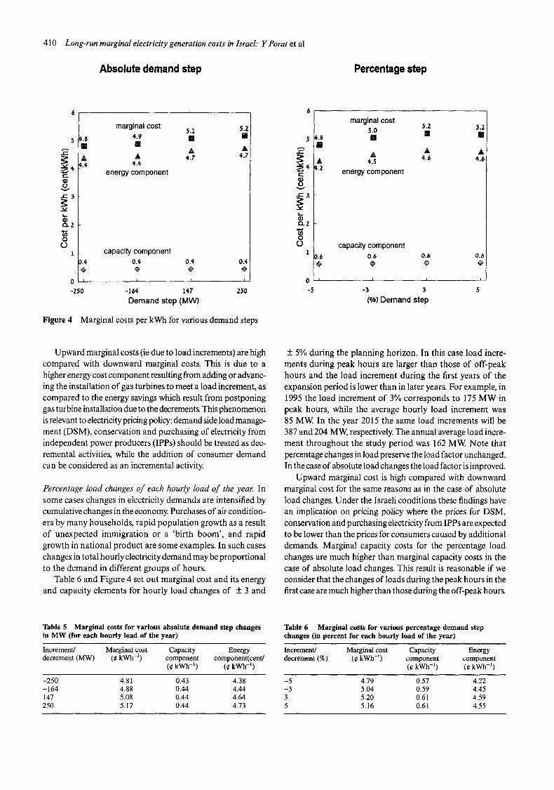
Figure 4 Marginal costs per kWh for various demand steps

~ 3

L$ ==

A ;.2

¢3.2

o

1 ~ .6

0 I

-5

marginal cost LZ 5.0 []

[]

& A 4.6

T.S

energy component

5.2 B

A 4.6

capacity component 0.6 0.6 0.6

f I I

-3 3 (%) Demand step

Upward marginal costs (ie due to load increments) are high compared with downward marginal costs. This is due to a higher energy cost component resulting from adding or advanc- ing the installation of gas turbines to meet a load increment,-as compared to the energy savings which result from postponing gas turbine installation due to the decrements, This phenomenon is relevant to electricity pricing policy: demand side load management (DSM), conservation and purchasing of electricity from independent power producers (IPPs) should be treated as decremental activities, while the addition of consumer demand can be considered as an incremental activity.

Percentage load changes of each hourly load of the year. In some cases changes in electricity demands are intensified by cumulative changes in the economy. Purchases of air condition- ers by many households, rapid population growth as a result of unexpected immigration or a 'birth boom', and rapid growth in national product are some examples. In such cases changes in total hourly electricity demand may be proportional to the demand in different groups of hours.

Table 6 and Figure 4 set out marginal cost and its energy and capacity elements for hourly load changes of + 3 and

+ 5% during the planning horizon. In this case load increments during peak hours are larger than those of off-peak hours and the load increment during the first years of the expansion period is lower than in later years. For example, in 1995 the load increment of 3% corresponds to 175 MW in peak hours, while the average hourly load increment was 85 MW. In the year 2015 the same load increments will be 387 and 204 MW, respectively. The annual average load increment throughout the study period was 162 MW. Note that percentage changes in load preserve the load factor unchanged. In the case of absolute load changes the load factor is improved.

Upward marginal cost is high compared with downward marginal cost for the same reasons as in the case of absolute load changes. Under the Israeli conditions these findings have an implication on pricing policy where the prices for DSM, conservation and purchasing electricity from IPPs are expected to be lower than the prices for consumers caused by additional demands. Marginal capacity costs for the percentage load changes are much higher than marginal capacity costs in the case of absolute load changes. This result is reasonable if we consider that the changes of loads during the peak hours in the first case are much higher than those during the off-peak hours.

Table 5 Marginal costs for various absolute demand step changes in MW (for each hourly load of the year)

Increment/ Marginal cost Capacity Energy decrement (MW) (¢ kWh -~) component component(cent/

(¢ kWh -t) (¢ kWh -t)

-250 4.81 0.43 4.38 -164 4.88 0.44 4.44 147 5.08 0.44 4.64 250 5.17 0.44 4.73

Table 6 Marginal costs for various percentage demand step changes (in percent for each hourly load of the year)

Increment/ Marginal cost Capacity Energy decrement (%) (¢ kWh -t) component component

(¢ kWh -t) (¢ kWh -t )

- 5 4.79 0.57 4.22 -3 5.04 0.59 4.45 3 5.20 0.61 4.59 5 5.16 0.61 4.55


Summary and conclusions

This paper presents two methods for calculating long-run marginal generation costs, both based on generation expansion planning models. The first method calculates total long- run marginal cost for different hourly demand groups: peak, shoulder and off-peak demands. The second method does not deal with each separately, but uses a more elaborate approach to energy costs: its calculated long run marginal capacity cost is allocated over the hours of each year according to the unsupplied energy distribution. Under optimal conditions, marginal capacity cost should equal the loss of load costs.

For tariff purposes, the first method may be preferable in presenting real generation planning marginal costs, and its use is recommended for time-of-use pricing, tariffs for private producers including backup prices, and for demand side load management. The second method could be used as an approximation when there is similarity between the marginal costs resulting from the two methods. However, the second method, which apportions capacity cost proportionately to unsupplied energy, is relevant to pricing if the demand elastic- ity in each of the nine periods is equal.

Uncited references

International Atomic Energy Agency (1984); Vardi and Avi- Itzhak (1981)

References

Andersson, R and Bohman, M (1985) Short- and long-run marginal cost pricing: on their alleged equivalence. Energy Econ. October, 279-288.

Crew, M, and Kleindorfer, P (1986) The Economics of Public Utility Regulation MIT Press, Cambridge, MA

Dickson, C, and Chamberlin, J (1984) 'The design of alternative rates for public power systems: issues and procedures' EPRI EA-3609, Palo-Alto, CA

Fogel Committee (1991) 'Report of the Committee for the examination of electricity tariffs in Israel' Ministry of Finance and Ministry lbr Energy and Infrastructure

Goett, A A, McFadden, D and Woo C K (1988) Electricity reliability special issue. Energy J 9, 105

Hall, G C, Healy, M T, and Poland, W B (1986) 'PG and E's new methodology for value-based generation reliability planning' Pacific Gas and Electric Co. Presentation to Edison Electric Institute

Kottik, D, Blau, M and Frank, Y (1995) Reliability of supply to the consumers as function of the installed generation reserve margin. Elec. Power Sys. Res. 33, 63-67.

Levin, N, and Zahavi, J (1986) Marginal and Production Costing Model for Electricity, Accounting for Uncertainty, Maintenance, Require- ments and Unit Commitment Program User's Guide Version 2.0, Tel- Aviv University, Tel Aviv

MIT Energy Laboratory (1982) 'Electric generation expansion analysis system (EGEAS)' EPRI EL-2561, Final Report

Mosinzon, R (1981) 'Optimal division to seasonal hourly demand groups for TOU pricing' Ministry of Energy and Infrastructure, Jerusalem, Israel

P PLUS Corporation, PWEEK Module (1993) 'Hourly chronological production simulation model' Version 5.0, Cupertino, CA

Sanghvi, A P (1986) 'Economic costs of electricity supply interruptions: U.S. and foreign experiences, the value of service reliability to custom- ers' EPRI EA-4494

Turvey R (1968) Optimal Pricing and Investment in Electricity Supply Allen and Anwing, London

Turvey, R, and Anderson, D (1977) Electrici O, Economics John Hop- kins University Press, Baltimore, MD

Vardi, J, and Avi-Itzhak, B (1981) Electric Energy Generation MIT Press, Cambridge, MS

Vardi, J, Zahavi, J and Avi-ltzhak, B (1977) Variable load pricing in the face of loss of load probability. Bell J. Econ. 8, 270-286.

Wenders, J (1976) Peak load pricing in the electric utility industry. Bell J Econ. 7, 232-241.

Woo, C K, and Pupp, R L (1991) 'Cost of service distributions to electricity consumers' City Polytechnic of Hong Kong

Zahavi, J, and Feiler, D (1979) Time of Day Costing of Electricity. Program U~er's Guide, Tel-Aviv University, TeI-Aviv

long-run marginal electricity generation costs in israel

Documents