logistic regression modelling for first- and second- …geoff-morrison.net/documents/morrison (2007)...

* The writing of this chapter was supported by the Social Sciences and Humanities Research

Council of Canada. My thanks to Terrance M. Nearey, the editors, and anonymous reviewers forcomments and advice.1 Now at Boston University.

2 Although less flexible, another suitable method is probit analysis.

LOGISTIC REGRESSION MODELLING FOR FIRST- AND SECOND-

LANGUAGE PERCEPTION DATA*

GEOFFREY STEWART MORRISONUniversity of Alberta1

Abstract

Logistic regression analysis has, for some time, been successfully applied to L1 speechperception data, but has not been widely applied in L2 speech perception research. Thischapter is a tutorial which makes use of simple data sets to introduce logistic regressionanalysis as applied to categorical response data from L1 and L2 speech perceptionexperiments. Data are taken from an experiment on L1 Spanish vowel perception byÁlvarez González, and experiments on L1 and L2 English vowel perception byEscudero & Boersma and Morrison. Model fitting is demonstrated as a technique todetermine which acoustic cues are attended to by listeners. Logistic regressioncoefficients are used to quantify how listeners use those acoustic cues, to producegraphical representations of their use of acoustic cues, and as statistics in secondaryanalyses used to determine whether there are significant differences in the perceptionof stimuli by L1 versus L2 groups of listeners.

1. Introduction

Logistic regression is a statistical method suitable for analysing identificationresponse data from speech perception experiments.2 Although logistic regressionhas, for some time, been applied successfully in first-language (L1) speechperception research (e.g., Benkí 2001; Breier et al. 2001; de Jong, Lim & Nagao2004; Maddox, Molis, & Diehl 2002; Nearey 1990, 1997, Rosen & Manganari2001), it has not been widely applied in second-language (L2) speech perception

Geoff

Text Box

A revised version of this manuscript appears as: Morrison, G. S. (2007). Logistic regression modelling for first- and second-language perception data. In M. J. Solé, P. Prieto, & J. Mascaró(Eds.), Segmental and prosodic issues in Romance phonology (pp. 219–236). Amsterdam: John Benjamins.

2 GEOFFREY STEWART MORRISON

research. This chapter is intended to be an introduction to understanding logisticregression applied to L1 and L2 speech perception data, and is aimed especiallyat L2-speech-perception students and researchers who are not familiar with thetechnique. Using relatively simple data sets, I will illustrate some of the ways inwhich logistic regression can be applied. Readers should then find it easier tounderstand the more complex analyses in L1 perception papers such as Nearey(1990, 1997) and L2 perception papers such as Morrison (2005b, 2006). Forgeneral introductions to applied logistic regression see Hosmer & Lemeshow(2000), Menard (2001), and Pampel (2000).

2. Fitting a logistic regression model

2.1 One stimulus dimension, binomial responses

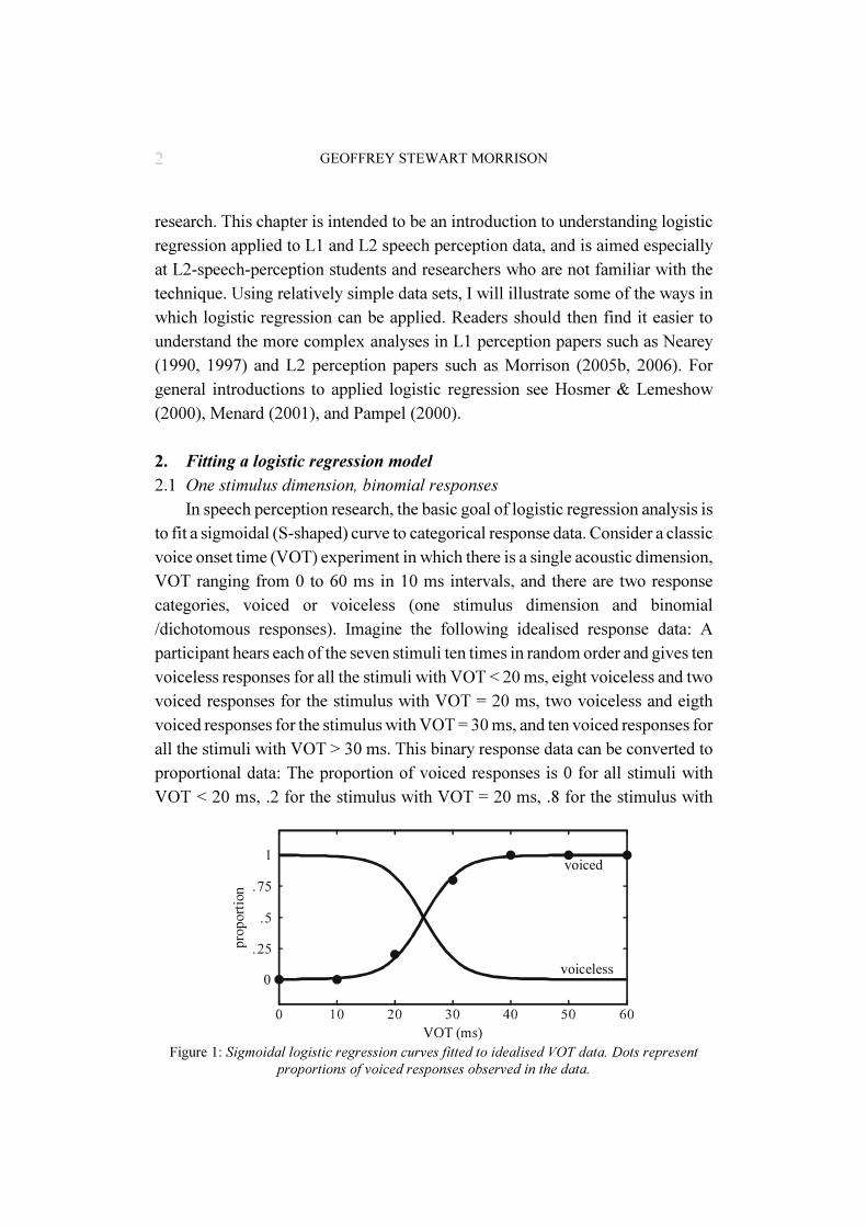
In speech perception research, the basic goal of logistic regression analysis isto fit a sigmoidal (S-shaped) curve to categorical response data. Consider a classicvoice onset time (VOT) experiment in which there is a single acoustic dimension,VOT ranging from 0 to 60 ms in 10 ms intervals, and there are two responsecategories, voiced or voiceless (one stimulus dimension and binomial/dichotomous responses). Imagine the following idealised response data: Aparticipant hears each of the seven stimuli ten times in random order and gives tenvoiceless responses for all the stimuli with VOT < 20 ms, eight voiceless and twovoiced responses for the stimulus with VOT = 20 ms, two voiceless and eigthvoiced responses for the stimulus with VOT = 30 ms, and ten voiced responses forall the stimuli with VOT > 30 ms. This binary response data can be converted toproportional data: The proportion of voiced responses is 0 for all stimuli withVOT < 20 ms, .2 for the stimulus with VOT = 20 ms, .8 for the stimulus with

0

.25

.5

.75

1

VOT (ms)

proportion

voiceless

voiced

Figure 1: Sigmoidal logistic regression curves fitted to idealised VOT data. Dots representproportions of voiced responses observed in the data.

3LOGISTIC REGRESSION MODELLING

3 The number of residual degrees of freedom is the number of independent pieces of information

in the model. For the models here, this is the number of stimuli multiplied by one less than thenumber of response categories, minus the number of non-redundant coefficients estimated in themodel. (Since the responses are proportions, they must sum to 1, and the proportions for the lastcategory are redundant.) There are 7 stimuli and 2 response categories in the VOT data, and 2coefficients/parameters in the logistic regression model fitted to the data; therefore there are 5residual degrees of freedom in the model.4 I follow Nearey (1990, 1997) in the use of the symbols G2 for deviance and ΔG2 for the difference

in the deviance between two nested models (see below). Hosmer & Lemeshow (2000) use D forthe former and G for the latter. Menard (2002) uses D

M for the former, and G

M for the latter if the

smaller model is the bias-only model, but Gk for other pairs of models.

VOT = 30 ms, and 1 for all stimuli with VOT > 30 ms. The observed proportionsof voiced responses are plotted in Figure 1, as are the sigmoidal curves fitted viaa logistic regression analysis to the proportions of voiced and voiceless responses.

The fitted curves are not a perfect fit to the data; for example, the predictedprobability of a voiced response at 20 ms is .172 rather than the observed value of.2. However, the curve is generally very close to the data points. Goodness-of-fitcan be assessed in several ways. A standard method is to measure the distancebetween the observed and predicted values for each stimulus and take an averageover all the stimuli: Root-mean-squared (RMS) error is the sum of the squares ofthe differences between the observed and predicted values (sum of squared errors),divided by the residual degrees of freedom in the model, then square rooted.3 RMSerror can be scaled by the number of responses per stimulus to give a percentageroot-mean-squared error (%RMS). The RMS error for the logistic regressionmodel fitted to the data in Figure 1 is 2.6%. Another measure of goodness-of-fitis the percentage modal agreement (%MA), the percentage of times, over all thestimuli, that the most likely response predicted by the model matches the mostcommon (the modal) response of the listener. If getting the category right is whatcounts, then %MA may be a more meaningful measure. The MA for the logisticregression model fitted to the data in Figure 1 is 100%. The goodness-of-fitmeasure actually used when fitting logistic regression models is the deviancestatistic G2, which is determined as follows: For each response category at eachstimulus, calculate the natural logarithm of the model’s predicted value for theresponse category divided by the natural logarithm of the value of the observedresponse for that category and multiplied by the value of the observed response,then sum over all categories and stimuli and multiply by minus two. Compared toRMS error, the G2 statistic is less intuitively meaningful, but, like RMS error, itdecreases as goodness-of-fit improves.4

Several factors can affect goodness-of-fit. One factor is the appropriateness


5 The use of pooled data obscures individual differences which increase the variance in the data,

and the assumption of independence of observations is violated. Given these issues, and the lackof consensus on an appropriate approach to repeated measures data in this type of analysis, someresearchers do not believe that pooling can be justified. In some instances, multi-level modellingmay be applied (see Quené & van den Burgh 2004).

of the model: Clearly the sigmoidal curve of a logistic regression model is a betterfit to our data than would be the straight line of a linear regression model. In somecases the appropriateness of the model, or lack thereof, may not be so apparent,an issue which Hosmer & Lemeshow (2000: §5.3) discuss in detail. For formantvalues in vowel stimuli, goodness-of-fit typically improves when frequency isentered into the model in log Hertz (or mel, Bark, or ERB) rather than in Hertz.Since human frequency perception is closer to logarithmic rather than linear, amodel fitted to log Hertz values is usually more appropriate than a model fitted toHertz values. Another factor which can decrease goodness-of-fit is noise in thedata: If the listener is occasionally distracted, they may fail to hear a stimulus andpress a response button at random. A certain number of responses in the data willthen be from a random distribution which does not reflect the listener’s perceptionof the stimuli. If the number of random responses is relatively small, they mayhave relatively little effect on the location and shape of the fitted curve; however,the random responses will likely cause the observed values for some stimuli to befurther from the curve than they would otherwise have been, and so will decreasethe goodness-of-fit (noise will also usually cause the slopes of the curves to beshallower). Yet another factor that can decrease goodness-of-fit, is the use of datapooled across listeners. It could be that a logistic regression model fits eachindividual’s data well, but that the exact location of the category boundaries varyacross listeners, and hence the boundaries in the pooled data are fuzzier than eachindividual listener’s boundaries. Although problematic for statistical analysis,5 useof pooled data may be justified on linguistic grounds: If the listeners are all nativespeakers of the same dialect then it may be argued that they will have similarpronunciation and perception patterns, and any interlistener differences will benegligible for communication purposes. A population average model based ondata pooled across listeners may reasonably be taken to characterise the perceptionof a group of native speakers of a given dialect.

2.2 Multiple stimulus dimensions, multinomial response categories

Let us look at some data from an actual experiment. Álvarez González (1980:Ch. 3) investigated L1-Spanish listeners’ perception of a synthetic vowel space in


6 The software is available as Matlab code upon request from T. M. Nearey (current e-mail:

[email protected]), or, along with additional code to run the analyses describe in this paper,from G. S. Morrison (current website: http://cns.bu.edu/~gsm2). With some additional effort, mostof the analyses described below could also be conducted using commercial software such as SPSSor STATA, or free software such as R.7 Non-linear probability values can be transformed into linear logit values (see Pampel, 2000: Ch.

1). In the case of the VOT data, the odds of a voiced response is the ratio of the probability of avoiced response to the probability of a voiceless response odds(voiced) = p(voiced) / p(voiceless).The logit is the natural logarithm of the odds Logit(voiced) = log(odds(voiced)).8 Details of model fitting are beyond the scope of this tutorial. Interested readers may wish to

consult, in increasing depth of coverage, Pampel (2000), Hosmer & Lemeshow (2000), McCullagh& Nelder (1983), and Haberman (1979).

which F1 varied from 250–800 Hz in 9 steps (10 points), F2 varied from750–2700 Hz in 8 steps (9 points), and F3 varied from 2300–2900 Hz in 2 steps(3 points). The total number of stimuli was 231 rather than 270 since the cornerwhere F1 would have been higher than F2 was excluded. Fifty listeners heard eachstimulus once in random order in the context /_�a/, and responded by circlingorthographic ‘ara’, ‘era’, ‘ira’, ‘ora’, or ‘ura’ on an answer sheet, therebyidentifying each synthetic vowel as one of the Spanish vowels, /a/, /e/, /i/, /o/, or/u/. This constitutes three stimulus dimensions and five response categories.Álvarez González reported results pooled across participants.

We will use logistic regression analysis to answer three questions regardingthe Álvarez González data: Question 1: Does the listeners’ vowel perception depend on F1 and F2?

Question 2: Does the listeners’ vowel perception depend on F3 in additionto F1 and F2?

Question 3: How do F1 and F2 affect the listeners’ vowel perception?

The software that we will use to build logistic regression models ofmultinomial/polytomous response data was implemented by Terrance M. Neareybased on an algorithm described in Haberman (1979).6 Logistic regressionoperates in a logistic (log odds) space,7 and fits a model by maximising the G2

goodness-of-fit to the data using an iterative maximum likelihood technique. Thetechnique selects a set of estimated coefficient values that (given the constraintsof the model) result in the predicted values for each response category at eachstimulus being as close as possible to the observed values (the average errorbetween observed and predicted values is minimised over all the stimuli andcategories).8 For models that will be fitted to the Álvarez González data, the set


9 It is also possible to build more complex models including coefficients for quadratic square and

crossproduct terms, etc.

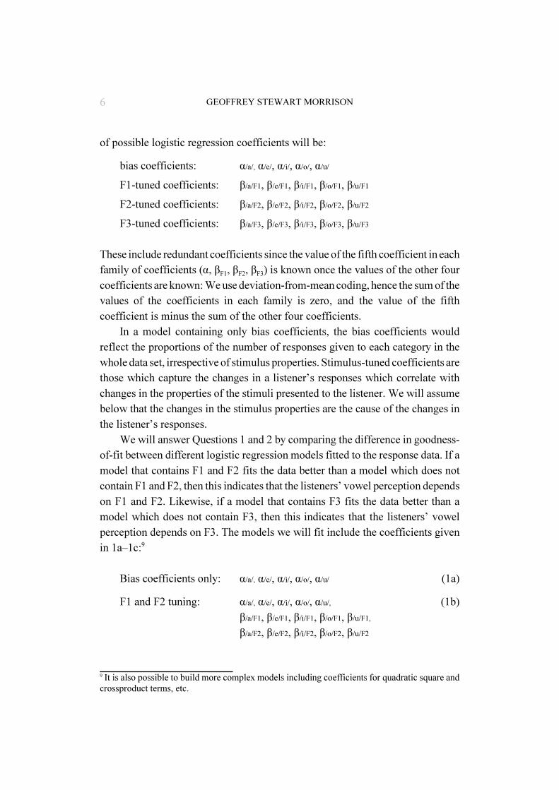
of possible logistic regression coefficients will be:

bias coefficients: α/a/, α/e/, α/i/, α/o/, α/u/

F1-tuned coefficients: β/a/F1, β/e/F1, β/i/F1, β/o/F1, β/u/F1



These include redundant coefficients since the value of the fifth coefficient in eachfamily of coefficients (α, βF1, βF2, βF3) is known once the values of the other fourcoefficients are known: We use deviation-from-mean coding, hence the sum of thevalues of the coefficients in each family is zero, and the value of the fifthcoefficient is minus the sum of the other four coefficients.

In a model containing only bias coefficients, the bias coefficients wouldreflect the proportions of the number of responses given to each category in thewhole data set, irrespective of stimulus properties. Stimulus-tuned coefficients arethose which capture the changes in a listener’s responses which correlate withchanges in the properties of the stimuli presented to the listener. We will assumebelow that the changes in the stimulus properties are the cause of the changes inthe listener’s responses.

We will answer Questions 1 and 2 by comparing the difference in goodness-of-fit between different logistic regression models fitted to the response data. If amodel that contains F1 and F2 fits the data better than a model which does notcontain F1 and F2, then this indicates that the listeners’ vowel perception dependson F1 and F2. Likewise, if a model that contains F3 fits the data better than amodel which does not contain F3, then this indicates that the listeners’ vowelperception depends on F3. The models we will fit include the coefficients givenin 1a–1c:9

Bias coefficients only: α/a/, α/e/, α/i/, α/o/, α/u/ (1a)

F1 and F2 tuning: α/a/, α/e/, α/i/, α/o/, α/u/, (1b)β/a/F1, β/e/F1, β/i/F1, β/o/F1, β/u/F1,

β/a/F2, β/e/F2, β/i/F2, β/o/F2, β/u/F2


10 The Pearson χ2: For each stimulus, the square of the difference between the observed values of

the responses and the model’s predicted values, then divided by the model’s predicted values, thensummed over all stimuli.11

McCullagh & Nelder (1983) advise using a fixed overdispersion, typically from the largest modelconsidered. The 1b versus 1a comparison would still be significant on the quasi-likelihood F testif the overdispersion from Model 1c were used.

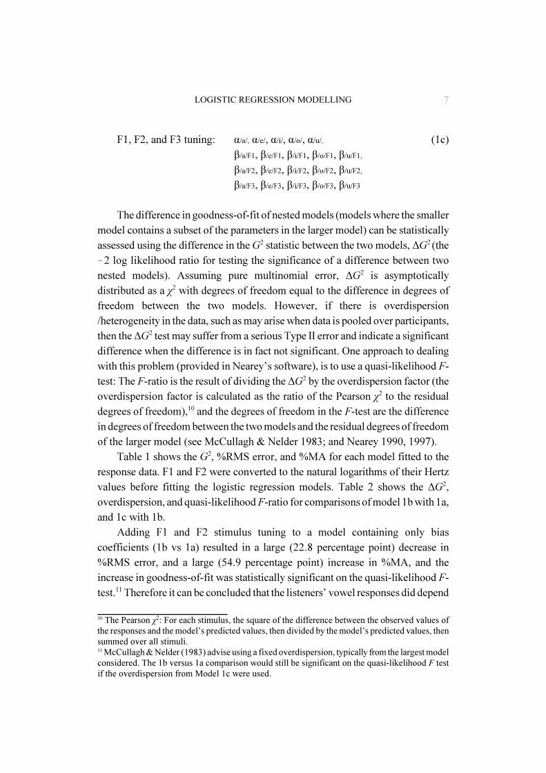
F1, F2, and F3 tuning: α/a/, α/e/, α/i/, α/o/, α/u/, (1c)β/a/F1, β/e/F1, β/i/F1, β/o/F1, β/u/F1, β/a/F2, β/e/F2, β/i/F2, β/o/F2, β/u/F2, β/a/F3, β/e/F3, β/i/F3, β/o/F3, β/u/F3

The difference in goodness-of-fit of nested models (models where the smallermodel contains a subset of the parameters in the larger model) can be statisticallyassessed using the difference in the G2 statistic between the two models, ΔG2 (the!2 log likelihood ratio for testing the significance of a difference between twonested models). Assuming pure multinomial error, ΔG2 is asymptoticallydistributed as a χ2 with degrees of freedom equal to the difference in degrees offreedom between the two models. However, if there is overdispersion/heterogeneity in the data, such as may arise when data is pooled over participants,then the ΔG2 test may suffer from a serious Type II error and indicate a significantdifference when the difference is in fact not significant. One approach to dealingwith this problem (provided in Nearey’s software), is to use a quasi-likelihood F-test: The F-ratio is the result of dividing the ΔG2 by the overdispersion factor (theoverdispersion factor is calculated as the ratio of the Pearson χ2 to the residualdegrees of freedom),10 and the degrees of freedom in the F-test are the differencein degrees of freedom between the two models and the residual degrees of freedomof the larger model (see McCullagh & Nelder 1983; and Nearey 1990, 1997).

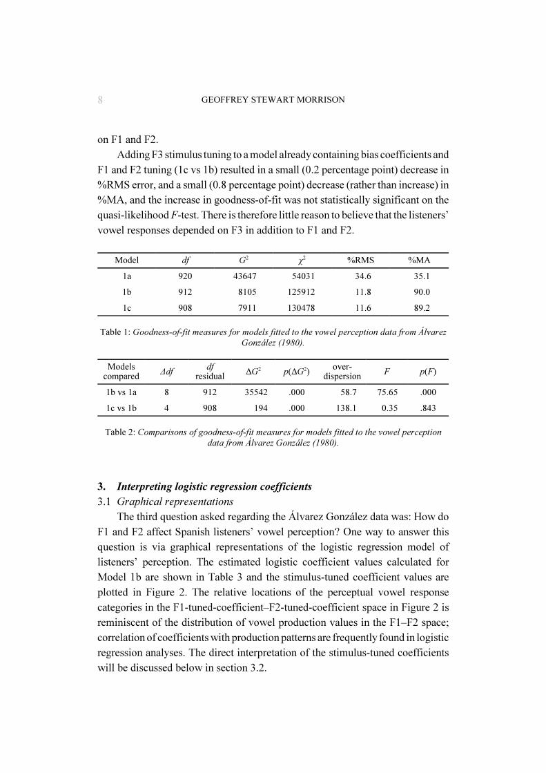
Table 1 shows the G2, %RMS error, and %MA for each model fitted to theresponse data. F1 and F2 were converted to the natural logarithms of their Hertzvalues before fitting the logistic regression models. Table 2 shows the ΔG2,overdispersion, and quasi-likelihood F-ratio for comparisons of model 1b with 1a,and 1c with 1b.

Adding F1 and F2 stimulus tuning to a model containing only biascoefficients (1b vs 1a) resulted in a large (22.8 percentage point) decrease in%RMS error, and a large (54.9 percentage point) increase in %MA, and theincrease in goodness-of-fit was statistically significant on the quasi-likelihood F-test.11 Therefore it can be concluded that the listeners’ vowel responses did depend


on F1 and F2. Adding F3 stimulus tuning to a model already containing bias coefficients and

F1 and F2 tuning (1c vs 1b) resulted in a small (0.2 percentage point) decrease in%RMS error, and a small (0.8 percentage point) decrease (rather than increase) in%MA, and the increase in goodness-of-fit was not statistically significant on thequasi-likelihood F-test. There is therefore little reason to believe that the listeners’vowel responses depended on F3 in addition to F1 and F2.

Model df G2 χ2 %RMS %MA

1a 920 43647 54031 34.6 35.1

1b 912 8105 125912 11.8 90.0

1c 908 7911 130478 11.6 89.2

Table 1: Goodness-of-fit measures for models fitted to the vowel perception data from ÁlvarezGonzález (1980).

Modelscompared Δdf df

residual ΔG2 p(ΔG2) over-dispersion F p(F)

1b vs 1a 8 912 35542 .000 58.7 75.65 .000

1c vs 1b 4 908 194 .000 138.1 0.35 .843

Table 2: Comparisons of goodness-of-fit measures for models fitted to the vowel perceptiondata from Álvarez González (1980).

3. Interpreting logistic regression coefficients

3.1 Graphical representations

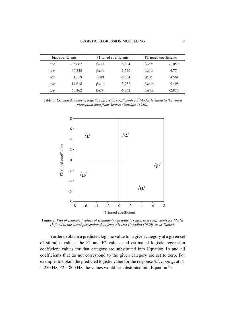
The third question asked regarding the Álvarez González data was: How doF1 and F2 affect Spanish listeners’ vowel perception? One way to answer thisquestion is via graphical representations of the logistic regression model oflisteners’ perception. The estimated logistic coefficient values calculated forModel 1b are shown in Table 3 and the stimulus-tuned coefficient values areplotted in Figure 2. The relative locations of the perceptual vowel responsecategories in the F1-tuned-coefficient–F2-tuned-coefficient space in Figure 2 isreminiscent of the distribution of vowel production values in the F1–F2 space;correlation of coefficients with production patterns are frequently found in logisticregression analyses. The direct interpretation of the stimulus-tuned coefficientswill be discussed below in section 3.2.


-8 -6 -4 -2 0 2 4 6 8

-8

-6

-4

-2

0

2

4

6

8

F1-tuned coefficient

F2-t

uned c

oeff

icie

nt

Figure 2: Plot of estimated values of stimulus-tuned logistic regression coefficients for Model1b fitted to the vowel perception data from Álvarez González (1980), as in Table 3.

In order to obtain a predicted logistic value for a given category at a given setof stimulus values, the F1 and F2 values and estimated logistic regressioncoefficient values for that category are substituted into Equation 1b and allcoefficients that do not correspond to the given category are set to zero. Forexample, to obtain the predicted logistic value for the response /u/, Logit/u/, at F1= 250 Hz, F2 = 800 Hz, the values would be substituted into Equation 2:

bias coefficients F1-tuned coefficients F2-tuned coefficients

α/a/ -35.667 β/a/F1 6.804 β/a/F2 -1.059

α/e/ -40.832 β/e/F1 1.240 β/e/F2 4.774

α/i/ 1.519 β/i/F1 -5.664 β/i/F2 4.561

α/o/ 14.618 β/o/F1 3.982 β/o/F2 -5.405

α/u/ 60.362 β/u/F1 -6.362 β/u/F2 -2.870

Table 3: Estimated values of logistic regression coefficients for Model 1b fitted to the vowelperception data from Álvarez González (1980).


Logit/u/ = α/u/ + β/u/F1×F1 + β/u/F2×F2 (2)

Logit/u/ = 60.362 !6.362×log(250) !2.870×log(800) = 6.050

The predicted probability for the response /u/, p/u/, is calculated as in Equation 3:

(3)p

e

e

Logit

Logit

x

x

/ /

/ /

u

u

=

∑

p/u/ = eLogit/u/ / (eLogit/a/ + eLogit/e/ + eLogit/i/ + eLogit/o/ + eLogit/u/)

p/u/ = e6.050 / (e!5.178 + e!2.073 + e0.734 + e0.474 + e6.050) = .991

where x takes on the values of all the response categories {/a/, /e/, /i/, /o/, /u/}:Each value of Logitx is calculated as in Equation 2 using the same F1 and F2values, and the estimated logistic regression coefficients appropriate for eachresponse category.

If a range of F1 and F2 values covering the stimulus space are substituted intoequations of the type given in Equations 2 and 3, the predicted probability of eachvowel response category can be calculated over the two-dimensional stimulusspace and plotted in a three-dimensional probability surface plot as in Figure 3.The height of a surface above the base of the plot indicates the predictedprobability of the response associated with that surface. The predicted probabilityof an /u/ response is close to 1 for low-F1–low-F2 values and decreasessigmoidally as either F1 or F2 or both increase. Response categories /i/, /e/, and/o/ have their highest predicted probabilities in the other corners of the stimulusspace. The predicted probability of an /a/ response is highest for high-F1 andintermediate-F2 values. The maximum predicted probability of an /a/ response isquite low compared to the maximum predicted probabilities of the other responsecategories (the number of /a/ responses in the raw data was low, this is not ananalytical error).

Figure 4 is a two-dimensional territorial map, it is equivalent to a view of thethree-dimensional probability surface plot (Figure 3) from directly above thestimulus plane. Only the response with the highest predicted probability is visiblein any part of the stimulus space. The solid lines represent the location of


Figure 3: Probability surface plot based on logistic regression Model 1b fitted to the vowelperception data from Álvarez González (1980). The height of a surface about the base of the

plot indicates the predicted probability of the corresponding response category.

250

334

447

598

800

750

1033

1423

1960

2700

0

.25

.5

.75

1

F1 (Hz)F2 (Hz)

probability

Figure 4: Territorial map based on logistic regression Model 1b fitted to the vowel perceptiondata from Álvarez González (1980).

250 334 447 598 800750

1033

1423

1960

2700

F2

(H

z)

F1 (Hz)


12 Rates of change for any category contrast can be calculated along any arbitrary line in the

stimulus space. For example, the rate of change from back vowel to front vowel identification asF2 increases: (β/i/F2 + β/e/F2) ! (β/u/F2 + β/o/F2) logit units per log Hertz. Or the rate of changefrom /i/ to /e/ for a one log Hertz increase in F1 and a two log Hertz decrease in F2: (β/e/F1 !2×β/e/F2) ! (β/i/F1 ! 2×β/i/F2) logit units per log Hertz.13

In the binomial case, one would usually use reference-category rather than deviation-from-meancoding. The coefficient values for one category would be fixed at zero and (what I have designated)the contrast coefficients would be the only coefficients reported by the software. If reference-category coding had been adopted in the multinomial model of the Álvarez González data, thereference category, e.g., /u/, would have been at the origin of Figure 2, and the other categorieswould have been shifted but would have maintained the same relative locations.14

The instantaneous value of the probability slope is the (partial) derivative of the probability withrespect to the dimension of interest. Using the binomial VOT example, this is: dp'dβVOT = β(voiced-

voiceless)VOT × p(voiced) × p(voiceless) (see Pampel 2000: 24). The steepest tangent occurs at theintersection between the lines/surfaces representing the probability of each category. In thebinomial case each category has a probability of .5 at the intersection, hence the instantaneous

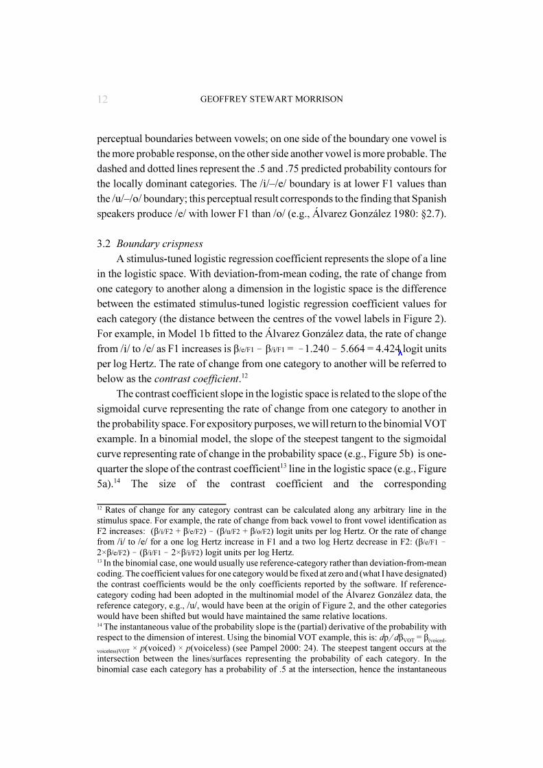
perceptual boundaries between vowels; on one side of the boundary one vowel isthe more probable response, on the other side another vowel is more probable. Thedashed and dotted lines represent the .5 and .75 predicted probability contours forthe locally dominant categories. The /i/–/e/ boundary is at lower F1 values thanthe /u/–/o/ boundary; this perceptual result corresponds to the finding that Spanishspeakers produce /e/ with lower F1 than /o/ (e.g., Álvarez González 1980: §2.7).

3.2 Boundary crispness

A stimulus-tuned logistic regression coefficient represents the slope of a linein the logistic space. With deviation-from-mean coding, the rate of change fromone category to another along a dimension in the logistic space is the differencebetween the estimated stimulus-tuned logistic regression coefficient values foreach category (the distance between the centres of the vowel labels in Figure 2).For example, in Model 1b fitted to the Álvarez González data, the rate of changefrom /i/ to /e/ as F1 increases is β/e/F1 ! β/i/F1 = !1.240 ! 5.664 = 4.424 logit unitsper log Hertz. The rate of change from one category to another will be referred tobelow as the contrast coefficient.12

The contrast coefficient slope in the logistic space is related to the slope of thesigmoidal curve representing the rate of change from one category to another inthe probability space. For expository purposes, we will return to the binomial VOTexample. In a binomial model, the slope of the steepest tangent to the sigmoidalcurve representing rate of change in the probability space (e.g., Figure 5b) is one-quarter the slope of the contrast coefficient13 line in the logistic space (e.g., Figure5a).14 The size of the contrast coefficient and the corresponding

Geoff

Cross-Out

Geoff

Replacement Text

This should read: 1.240 - (-5.664) = 6.904


slope at this point is: β(voiced-voiceless)VOT ×.5 × .5 = β(voiced-voiceless)VOT × .25. In multinomial cases, thecalculation of the slope of the maximum tangent to the sigmoidal rate-of-probability-change curvebetween two categories is complicated by the fact that other categories may have non-zeropredicted probabilities at the intersection of the two categories of interest, thus each category ofinterest will not have .5 probability at the intersection. However, a larger contrast coefficient valuewill still indicate a larger value for the maximum slope of a tangent to the sigmoidal curve.

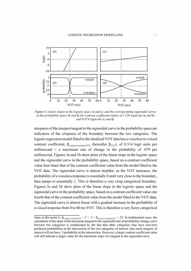
steepness of the steepest tangent to the sigmoidal curve in the probability space areindicators of the crispness of the boundary between the two categories. Thelogistic regression model fitted to the idealised VOT data has a voiceless to voicedcontrast coefficient, β(voiced-voiceless)VOT (hereafter βVOT), of 0.314 logit units permillisecond = a maximum rate of change in the probability of .079 permillisecond. Figures 5a and 5b show plots of the linear slope in the logistic spaceand the sigmoidal curve in the probability space, based on a contrast coefficientvalue four times that of the contrast coefficient value from the model fitted to theVOT data. The sigmoidal curve is almost steplike: as the VOT increases, theprobability of a voiceless response is essentially 0 until very close to the boundary,then jumps to essentially 1. This is therefore a very crisp categorical boundary.Figures 5c and 5d show plots of the linear slope in the logistic space and thesigmoidal curve in the probability space, based on a contrast coefficient value onefourth that of the contrast coefficient value from the model fitted to the VOT data.The sigmoidal curve is almost linear with a gradual increase in the probability ofa voiced response from 0 to 60 ms VOT. This is therefore a very fuzzy categorical

-10

-5

0

5

10

0 10 20 30 40 50 60

0

.25

.5.75

1

VOT (ms)

probability

logits

0 10 20 30 40 50 60

VOT (ms)

(a)

(b)

(c)

(d)

voiceless

voiced

voiceless

voiced

Figure 5: Linear slopes in the logistic space (a and c) and the corresponding sigmoidal curvesin the probability space (b and d) for contrast coefficient values of 1.256 logits/ms (a and b)

and 0.079 logits/ms (c and d).


boundary.Measures of boundary crispness or fuzziness are useful when analysing L2

perception data. Native speakers typically have crisp boundaries betweencategories, similar to Figure 5b. L2 learners may not have L1 categoriesdistinguished by the same acoustic cues as the L2 categories, the L1 may not usean acoustic dimension that is used in the L2, or the range of values sampled alongthe dimension may all fall within a single L1 category. In such cases, the L2learners would be expected to have very fuzzy boundaries, similar to Figure 5d.Even though their L1 may not provide them with a crisp categorical boundary,they may still be able to hear differences along the acoustic dimensions understudy and respond in a gradient manner, e.g., giving more voiced responses forlonger VOT, and thus have a non-zero contrast coefficient. As they learn the L2,they would be expected to approximate the perception of native speakers of theL2, their categorical boundaries would become crisper, and this would be reflectedin the contrast coefficient values from logistic regression models fitted to theirperception data.

3.3 Polar-coordinate contrast coefficients

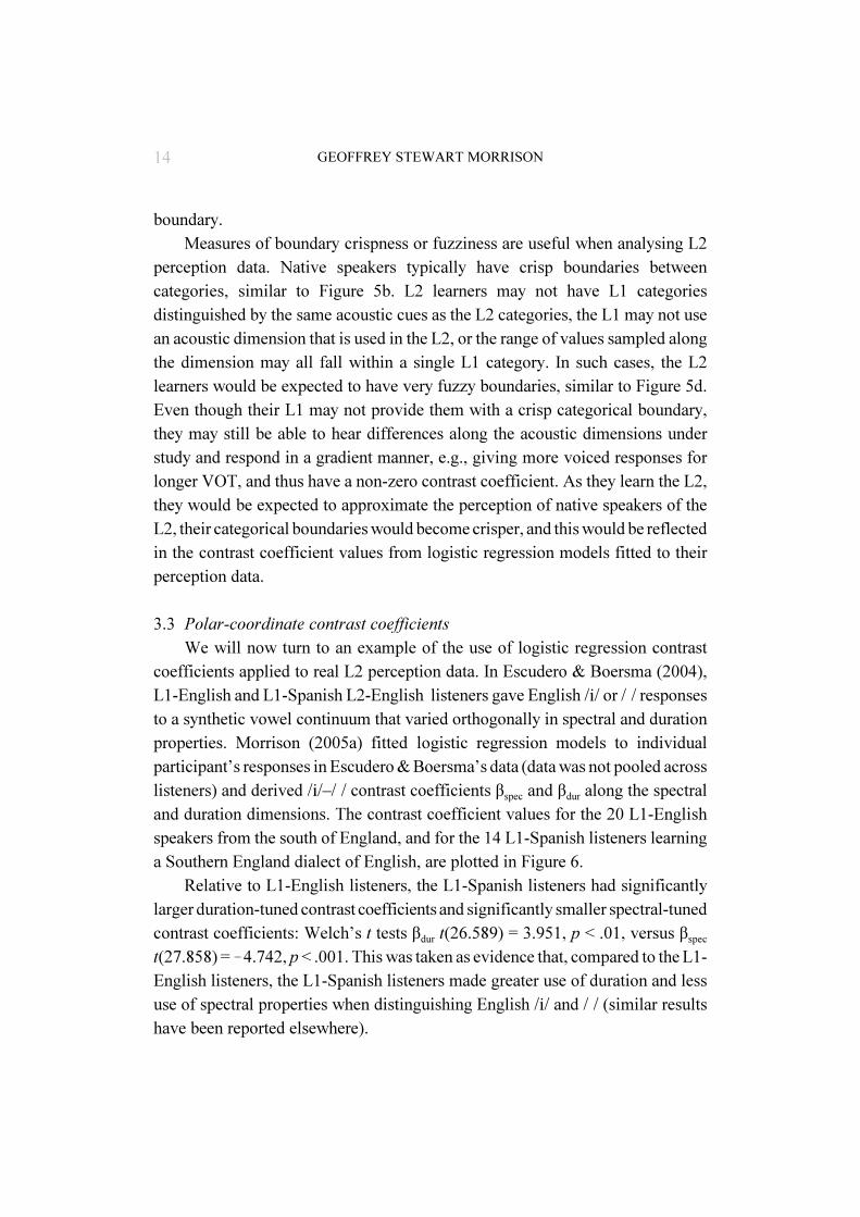
We will now turn to an example of the use of logistic regression contrastcoefficients applied to real L2 perception data. In Escudero & Boersma (2004),L1-English and L1-Spanish L2-English listeners gave English /i/ or /�/ responsesto a synthetic vowel continuum that varied orthogonally in spectral and durationproperties. Morrison (2005a) fitted logistic regression models to individualparticipant’s responses in Escudero & Boersma’s data (data was not pooled acrosslisteners) and derived /i/–/�/ contrast coefficients βspec and βdur along the spectraland duration dimensions. The contrast coefficient values for the 20 L1-Englishspeakers from the south of England, and for the 14 L1-Spanish listeners learninga Southern England dialect of English, are plotted in Figure 6.

Relative to L1-English listeners, the L1-Spanish listeners had significantlylarger duration-tuned contrast coefficients and significantly smaller spectral-tunedcontrast coefficients: Welch’s t tests βdur t(26.589) = 3.951, p < .01, versus βspec

t(27.858) = !4.742, p < .001. This was taken as evidence that, compared to the L1-English listeners, the L1-Spanish listeners made greater use of duration and lessuse of spectral properties when distinguishing English /i/ and /�/ (similar resultshave been reported elsewhere).


15 angle = arctan(βspec'βdur) magnitude = o&&&&&&&βspec

2 + βdur2

Boersma & Escudero (2005) pointed out that, because of constraints imposedby the edges of the stimulus space, the spectrally-tuned and duration-tunedcontrast coefficients were partially correlated, and recommended using the ratioof the two contrast coefficients in the same manner as Escudero & Boersma(2004) had used the ratio of their spectral and duration reliance measures. Theratio of the spectrally-tuned and duration-tuned contrast coefficients gives theorientation of the /i/–/�/ boundary in the spectral–duration stimulus space, i.e., theorientation of the boundary line on a territorial map (the ratio is a gradient, whichmay be converted to an angle in degrees). However, rather than simply taking theratio, the two contrast coefficients can be converted into polar coordinates toprovide orthogonal measures of: (1) the orientation of the boundary in thespectral–duration stimulus space, polar-coordinate angle; and (2) the boundarycrispness, polar-coordinate magnitude.15 The boundary crispness is the rate ofchange from one category to the other in the direction perpendicular to theorientation of the boundary. Two listeners could have identical boundaryorientations, but one could have a crisp and the other a fuzzy boundary. Lookingat boundary orientation alone would ignore this important difference in thelisteners’ perception, which could signal, for example, that the first listener has a

-0.25

0.00

0.25

0.50

0.75

-1 0 1 2

L1-SpanishL1-English

βdur

βspec

Figure 6: Contrast coefficients values from logistic regression models fitted to individualparticipant data from Escudero & Boersma (2004).


well established categorical boundary, and the second listener is responding towithin-category acoustic differences.

The use of polar coordinates provides relatively intuitive numericaldescriptors for the boundary. Figures 7a–7c provide probability surface plotswhich give examples of different boundary angles and magnitudes (the values arereported in the caption). Note the differences in the steepness of the curvedsurfaces reflecting differences in boundary crispness, and the differences in theorientation of the intersection between the curved surfaces reflecting boundaryorientation. (The angles were calculated such that an angle of 90° would indicatethat the listener used only spectral cues, and an angle of 0° would indicate that thelistener used only duration cues.)

Comparing the two groups in Escudero & Boersma’s data, the L1-Spanish L2-English listeners’ /i/–/�/ boundary angles were significantly smaller than those ofthe L1-English listeners, t(32) = 5.503, p < .001, indicating a relatively greater useof duration cues. On the other hand, the L1-Spanish L2-English listeners’ /i/–/�/

(a)

(b) (c)

Figure 7: Probability surface plots illustrating different boundary angles and magnitudes.(a) L1-English listener, angle 70° magnitude 0.88(b) L2-English listener, angle 27° magnitude 0.35(c) L2-English listener, angle !2° magnitude 0.46


boundary magnitudes were not significantly smaller than those of the L1-Englishlisteners, t(32) = 1.367, p = .181. Again we conclude that, compared to the L1-English listeners, the L2-English listeners made greater use of duration, but we didnot find statistical evidence that, as a group, the L2 learners had fuzzierboundaries.

3.4 Additional example of the use of contrast coefficients

Like Escudero & Boersma (2004), Morrison (2005b) investigated L1-SpanishL2-English listeners’ perception of the English /i/–/�/ contrast; however, in thelatter study the dialect of English was General Canadian English and the studysimultaneously assessed vowel and consonant perception. Listeners gave English/bit/, /bid/, /b�t/, /b�d/, /b�t/, and /b�d/ responses to stimuli from a resynthesisednatural speech continuum in which the vowels varied orthogonally in spectral andduration properties. A diphone-biassed logistic regression model (see Nearey1990, 1997) was fitted to each individual participant’s response data:

Segment bias coefficients: α/i/, α/�/, α/�/, α/t/, α/d/ (4)

Diphone bias coefficients: α/it/, α/id/, α/�t/, α/�d/, α/�t/, α/�d/

Stimulus-tuned coefficients: β/i/spec, β/�/spec, β/�/spec, β/t/spec, β/d/spec, β/i/dur, β/�/dur, β/�/dur, β/t/dur, β/d/dur

Participants were grouped via a hierarchical cluster analysis on the contrastcoefficient values β(/i/-/�/)spec, β(/i/-/�/)dur, β(/d/-/t/)spec and β(/d/-/t/)dur, and on the basis of the

crispness of their categorical boundaries the groups of L1-Spanish listeners were

assigned to a modified version of Escudero’s (2000) hypothesised stages of development

for L1-Spanish listeners learning the English /i/–/�/ contrast:

Stage 0 no ability to distinguish the contrast

Stage ½ category-goodness assimilation to Spanish /i/

Stage 1 distinguished via duration cues

Stage 2 distinguished via a mixture of duration and spectral cues

Stage 3 native-English-like perception, distinguished primarily on the basis of

spectral cues

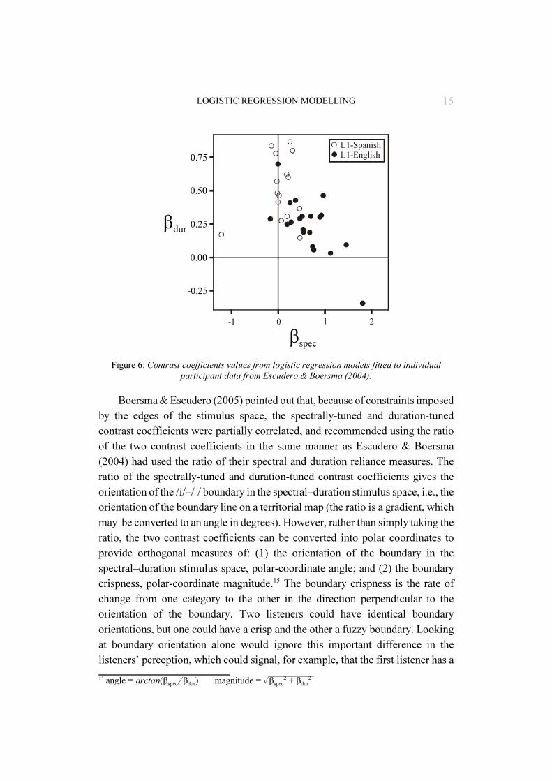
The values of individual participant’s contrast coefficients and their assignments to

stages of development are plotted in Figure 8. The hypothesised progression along the

stages of development is represented by the arrow. The contiguity of the hypothesised


stages along the arrow is a necessary condition for them to represent a developmental

sequence.

Figure 8: Contrast coefficients from logistic regression models fitted to individual participantdata from Morrison (2005b). Arrow joins contiguous groups of L1-Spanish listeners and

represents a hypothesised developmental path.

4. Conclusion

This chapter introduced logistic regression analysis as applied to the type ofcategorical response data typically collected in speech perception experiments inwhich listeners are asked to identify synthetic stimuli in terms of the speech-soundcategories. Comparison of the goodness-of-fit of different logistic regression

0.25

0.50

0.75

1.00

1.25

-20246

-0.5

0

0.5

1.0

1.5

-3.61 -1.61 0.40

L1-SpanishStage 0Stage ½Stage 1Stage 2Stage 3

L1-English


models was demonstrated as a means of determining which acoustic cues listenersused when identifying stimuli. This chapter also demonstrated the use of logisticregression coefficients to describe listeners’ perceptual use of acoustic cues.Logistic regression coefficients were used to produce detailed graphicalrepresentations of listeners’ use of perceptual cues. They provided a metric ofintercategory boundary orientation and crispness. They were also used as statisticsin secondary analyses which tested the differences in perception between L1 andL2 groups. Given that synthetic-stimuli category-identification experiments arecommon in L2 speech perception research, there is great potential for theapplication of logistic regression analysis to this field of research. I hope that thischapter has helped readers not previously familiar with the technique to gain abasic understanding of applied logistic regression analysis.

References

Álvarez González, Juan Antonio. 1980. Vocalismo español y vocalismo inglés.Ph.D. Dissertation, Universidad Computense de Madrid.

Benkí, José R. . 2001. “Place of Articulation and First Formant Transition PatternBoth Affect Perception of Voicing in English”. Journal of Phonetics 29.1–22.

Boersma, Paul, & Paola Escudero. 2005. “Measuring Relative Cue Weighting: Areply to Morrison”. Studies in Second Language Acquisition 27. 607–617.

Breier, Joshua I., Lincon Gray, Jack M. Fletcher, Randy L. Diehl, Patricia Klaas,Barbara R. Foorman, & Michelle R. Mollis. 2001. “Perception of Voice andTone Onset Time Continua in Children with Dyslexia and Without AttentionDeficit/hyperactivity Disorder”. Journal of Experimental Child Psychology

80. 245–270.Escudero, Paola. 2000. Developmental patterns in the adult L2 acquisition of new

contrasts: The acoustic cue weighting in the perception of Scottish tense/lax

vowels by Spanish speakers. MA thesis, University of Edinburgh.––––––– & Paul Boersma. 2004. “Bridging the Gap Between L2 SpeechPerception Research and Phonological Theory.” Studies in Second Language

Acquisition 26. 551–585. Haberman, Shelby J. 1979. Analysis of Qualitative Data. Vol. 2. New York:

Academic.Hosmer, David. W. & Stanley Lemeshow. 2000. Applied Logistic Regression. 2nd

ed. New York: Wiley.


de Jong, Kenneth J., Byung-jin Lim, & Kyoko Nagao. 2004. “The Perception ofSyllable Affiliation of Singleton Stops in Repetitive Speech”. Language and

Speech 47:3. 241–266.McCullagh, Peter & John A. Nelder. 1983. Generalized Linear Models. London:

Chapman and Hall.Maddox, W. Todd, Michelle R. Molis, & Randy L. Diehl. 2002. “Generalizing A

Neuropsychological Model of Visual Categorization to AuditoryCategorization of Vowels.” Perception & Psychophysics 64: 4. 584–597.

Menard, Scott. 2002. Applied Logistic Regression Analysis. Thousand Oaks, CA:Sage.

Morrison, Geoffrey Stewart. 2005a. “An Appropriate Metric for Cue Weightingin L2 Speech Perception: Response to Escudero & Boersma (2004)”. Studies

in Second Language Acquisition 27. 597–606.–––––––. 2005b. Development of L2 Vowel Perception and Production: L1-

Spanish speakers and the acquisition of the English /i/–/�/ contrast. Manuscriptsubmitted for publication.–––––––. 2006. L1 & L2 Production and Perception of English and Spanish

Vowels: A statistical modelling approach. PhD Dissertation, University ofAlberta.Nearey, Terrance M. 1990. “The Segment As A Unit of Speech Perception”.

Journal of Phonetics 18. 347–373.–––––––. 1997. “Speech Perception As Pattern Recognition”. Journal of the

Acoustical Society of America 101:6. 3241–3254. Pampel, Fred C. 2000. Logistic Regression: A primer. Thousand Oaks, CA: Sage.Quené, Hugo & Huub van den Bergh, 2004. “On Muli-Level Modelling of Data

from Repeated Measures Designs: A Tutorial”. Speech Communication 43.103–121.

Rosen, Stuart & Eva Manganari. 2001. “Is There a Relationship Between Speechand Non-speech Auditory Processing in Children With Dyslexia?” Journal

of Speech, Language, and Hearing Research 44. 720–736.

logistic regression modelling for first- and second- …geoff-morrison.net/documents/morrison (2007)...

Documents