LogGP: A Log-based Dynamic Graph Partitioning Method

Ning Xu †, Lei Chen ‡, Bin Cui †

†Key Lab of High Confidence Software Technologies (MOE), School of EECS, Peking University, China‡Hong Kong University of Science and Technology, Hong Kong, China

†{ning.xu, bin.cui}@pku.edu.cn, ‡leichen@cse.ust.hk

ABSTRACTWith the increasing availability and scale of graph data fromWeb 2.0, graph partitioning becomes one of efficient pre-processing techniques to balance the computing workload.Since the cost of partitioning the entire graph is strictlyprohibitive, there are some recent tentative works towardsstreaming graph partitioning which can run faster, be easilyparalleled, and be incrementally updated. Unfortunately,the experiments show that the running time of each parti-tioning is still unbalanced due to the variation of workloadaccess pattens during the supersteps. In addition, the one-pass streaming partitioning result is not always satisfactoryfor the algorithms’ local view of the graph.

In this paper, we present LogGP, a log-based graph parti-tioning system that records, analyzes and reuses the histor-ical statistical information to refine the partitioning result.LogGP can be used as a middle-ware and deployed to manystate-of-the-art paralleled graph processing systems easily.LogGP utilizes the historical partitioning results to gener-ate a hyper-graph and uses a novel hyper-graph streamingpartitioning approach to generate a better initial streaminggraph partitioning result. During the execution, the sys-tem uses running logs to optimize graph partitioning whichprevents performance degradation. Moreover, LogGP candynamically repartition the massive graphs in accordancewith the structural changes. Extensive experiments con-ducted on a moderate size of computing cluster with real-world graph datasets demonstrate the superiority of our ap-proach against the state-of-the-art solutions.

1. INTRODUCTIONData partitioning has been studied for decades. Recently,

with the scale of data from Internet becoming larger, datapartitioning, especially graph data partitioning has attractedmore and more attention. The unprecedented prolifera-tion of data from web requires efficient processing meth-ods to handle different workloads. Many parallelism frame-works have been proposed to process large-scale graphs, e.g.,

This work is licensed under the Creative Commons Attribution-NonCommercial-NoDerivs 3.0 Unported License. To view a copy of this li-cense, visit http://creativecommons.org/licenses/by-nc-nd/3.0/. Obtain per-mission prior to any use beyond those covered by the license. Contactcopyright holder by emailing info@vldb.org. Articles from this volumewere invited to present their results at the 40th International Conference onVery Large Data Bases, September 1st - 5th, 2014, Hangzhou, China.Proceedings of the VLDB Endowment, Vol. 7, No. 14Copyright 2014 VLDB Endowment 2150-8097/14/10.

Pregel, GraphLab and PowerGraph [17, 15, 11]. As otherdistributed systems, graph data partitioning is a key tech-nology to scale out computational capabilities.

Pregel [17], as one of the representative systems, devel-oped by Google, is based on the BSP (bulk-synchronousparallel) model and adopts a vertex-centric concept in whicheach vertex executes a user-defined function (UDF) in a se-quence of supersteps. By default, Pregel uses hash func-tion to distribute the vertices. Although hash partition-ing generates a well-balanced number of vertices across dis-tributed computing nodes, many messages have to be sentacross the nodes for updating which generates a huge com-munication cost.

Thus, some partitioning methods on Pregel-like systemswere proposed, most of which are based on k-balanced graphpartitioning [10]. K-balanced graph partitioning aims tominimize the total communication cost between computingnodes and balance the vertices on each partition. Andreevet al. [6] proved k-balanced graph partitioning is NP-Hard.Several approximation algorithms and multi-level heuristicalgorithms have been proposed. However, as the size ofgraph becomes larger, they all suffer from a significant in-crease of the partitioning time. As shown in [25], multi-levelapproach requires more than 8.5 hours to partition a graphfrom Twitter with approximately 1.5 billion edges whichis sometimes longer than the time spent on processing theworkload. Therefore recently, some works focused on muchsimpler streaming heuristics to get comparable result per-formance to multi-level ones with much shorter partitioningtime [23, 25]. Although the partitioning result balances thenumber of vertices among each node and reduces the com-munication cost, for many graph workloads in which not allvertices in every superstep will run the UDF, the stream-ing or even multi-level graph partitioning algorithms stillencounter the skewed running time for some workloads.

To deal with this issue, several approaches were recentlyproposed: Yang et al. [27] proposed a dynamic replicationbased partitioning with adaption to workload change. Shanget al. [21] investigated several graph algorithms and pro-posed simple yet effective policies that can achieve dynamicworkload balance. However, these approaches need to repar-tition the graph again whenever a new workload runs on itand there is no improvement on the partitioning results.In fact, the running statistics or historical partitioning logscan provide us useful information to refine the partitioningresult. In this paper, we investigate how to record, ana-lyze and reuse these statistics and logs to refine the graphpartitioning result. We settle the issue of the imbalance of

1917

running time and reduce the job running time by refiningthe graph partitioning quality. We develop a novel graphpartitioning management method - LogGP that reuses theprevious and running statistical information to refine thepartitioning. LogGP has two novel log-based graph parti-tioning techniques. LogGP first combines the graph andhistorical partitioning results to generate a hyper graph anduses a streaming based hyper graph approach to get a betterinitial partitioning result. When the workload is executing,LogGP then uses running statistics to estimate the runningtime of each node and reassigns the workload for the next su-perstep to reduce the superstep running time. To estimatethe running time of superstep, an innovative technique toprofile workload and graph is proposed. LogGP can be usedas a middle-ware and deployed to Pregel-like systems easily.

We implement LogGP on Giraph - an open source ver-sion of Pregel. The performance of LogGP is validated withseveral large graph datasets on different workloads. The ex-perimental results show that the proposed graph partition-ing approaches significantly outperform existing streamingapproaches and demonstrate superior scaling properties.

Our contributions in this paper can be summarized asfollows:

1. We identify an important running time imbalance prob-lem in large-scale graph processing system.

2. We design and implement LogGP to reuse the previ-ous and running statistics information for partitioningrefinement and propose Hyper Graph Repartitioningand Superstep Repartitioning techniques.

3. We conduct extensive experimental study to exhibitthe advantages of our approach.

The remaining of this paper is organized as follows. In Sec-tion 2, we review the problem of graph partitioning and rel-evant performance issues. In Section 3 and 4, we present thenovel Hyper Graph Repartitioning and Superstep Reparti-tioning techniques, followed by the architecture of LogGPin Section 5. Section 6 reports the findings of an extensiveexperimental study. Finally, we introduce the related workand conclude this paper in Section 7 and 8.

2. BACKGROUNDIn this section, we first introduce the Pregel system on

which our prototype system is built. We next introduce theproblem of graph partitioning and streaming graph parti-tioning. Finally, we analyze the graph partitioning problemin Pregel.

Pregel is a distributed graph processing system proposedby Google, based on the BSP (bulk-synchronous parallel)model [26]. In the BSP model, the graph processing job iscomputed via a number of supersteps separated by syn-chronization barriers. In each superstep, every worker, orcalled node, executes a user-defined function against a sub-set of the vertices on it in an asynchronous computing way.These vertices are called active vertices. The rest of ver-tices, which are not used in a superstep, are called inactivevertices. Besides, the node sends the necessary messagesto its neighbors for the following superstep. Once the com-munication and computation are finished, there is a globalsynchronization barrier to guarantee that all the nodes areready for next superstep or the assigned job is finished.

Same as the other distributed systems, to get best perfor-mance, workload should be assigned to each node equallywhile minimizing the communication cost. Thus graph par-titioning is an essential technology to get high scalability.

Graph Partitioning: We now formally describe the gen-eral graph partitioning problem. We use G = (V,E) to rep-resent the graph to be partitioned. V is a set of vertices,and E is a set of edges in the graph. The graph may beeither directed or undirected. Let Pk = {V1,...,Vk} be a setof k subsets of V . Pk is said to be a partition of G if: Vi 6=∅, Vi ∩ Vj = ∅, and ∪Vi = V , for i, j = 1, ..., k, i 6= j. Wecall the elements Vi of Pk the parts of the partition. Thenumber k is called the cardinality of the partition. In thispaper, we assume that each Vi is assigned to one computingnode, and use Vi denote the set of vertices in that node.

Graph partitioning problem is to find an optimal par-tition Pk based on an objective function. It is a combinato-rial optimization problem that can be defined as follows:

Definition 1. Graph partitioning problem can be definedfrom a triplet (S, p, f) such that: S is a discrete set of allthe partitions of G. p is a predicate on S which creates asubset of S called admissible solution set - Sp that all thepartitions in Sp is admissible for predicate p. f is the ob-jective function. Graph partitioning problem aims to find apartition P that P ∈ Sp and minimizes f(p):

f(P ) = minP∈Spf(P ) (1)

A simple policy is to partition the data with a hash func-tion, which is the default strategy applied in Pregel [17].However, this approach results in high communication costthus, degrades the performance. Some works use approx-imation or multi-level approaches to partition the graph.However as the graph becomes larger, the cost of partition-ing is unacceptable [25]. Thus, some recent works [23, 25]use streaming partitioning heuristics to partition the graph.

In particular, if the vertices of graph arrive in some orderwith the set of its neighbors, and we partition the graphbased on the vertex stream, it is called a Streaming GraphPartitioning Algorithm. Streaming graph partitioningalgorithm decides which part to assign for each incomingvertex. Once the vertex is placed, it will not be removed.

a. SSSP b. BFS

Figure 1: Running Time of Supersteps on a Node

These k-balanced graph partitioning approaches balancethe vertex computation job while the communication timeof each part is not considered. Thus, the running time,which contains both computation and communication time,of each node may be skew for each node. A reason for theimbalance is the Traversal-Style workload [21], e.g., SSSPand BFS. These workloads explore different active verticeson each node at different supersteps which is hard to pre-dict at the initial partitioning stage. Thus the computationtime and communication time of each node on specific su-persteps are imbalanced. Figure 1 shows the running time

1918

of a certain node for workloads SSSP and BFS with a multi-level graph partitioning algorithm for initial partitions. Wecan see that there is a significant running time imbalance foreach superstep. For the Always-Active workloads [21], thereis imbalance of running time as well, because the k-balancedgraph partitioning only balances the vertex computation jobwhile the communication time of each part is not considered.

The running imbalance of node for Pregel-like system af-fects the overall job running time for graph processing work-load and limits the scale out of the whole system. Thus,using static initial partitioning result which is generatedwithout analyzing the workload behavior cannot balance therunning time of each node.

To alleviate the issues mentioned above, we propose agraph partitioning scheme LogGP which exploits historicalgraph information. LogGP uses two novel techniques, i.e.,Hyper Graph Repartitioning and Superstep Repartitioning,which will be introduced in next two sections.

3. HYPER GRAPH REPARTITIONINGWe first introduce how to generate better initial partition-

ing result with the help of historical log. As mentioned inSection 1, multi-level partitioning algorithms are too slowfor large graphs. Thus, we use streaming approach to gen-erate initial partitioning result.

Let P t = V t1 , ..., V

tk be a partitioning result at time t,

where V ti is the set of vertices in partition i at time t. A

streaming graph partitioning is sequentially presented a ver-tex v and its neighbors N(v), and uses a streaming heuristicto assign v to a partition i only utilizing the informationcontained in the current partitioning P t. Although one-pass streaming partitioning algorithm has shorter partition-ing time, the partitioning result is not as good as multi-levelsolutions because it only has the information of the assignedvertices in the graph. In this paper, we use historical par-titioning log to enlarge the vision when running streaminggraph partitioning and refine the initial partitioning result.

We use two kinds of useful information that are providedby the historical partitioning result.

The first one is the last partitioning result of the samegraph or some parts of the graph. This result has dividedthe graph into several partitions generated by the streamingpartitioning algorithm. Although not optimized, it providesus a better initial input than random graph. We try toappropriately use this last partitioning result to provide thestreaming graph partitioning more information than that ofthe assigned vertices contained in the current partitioning.

The other information is the accessed active vertex setduring the execution of previous workloads which is calledLog Active Vertex Set(LAVS). A LAVS is an activevertex set that a node accessed in continuous supersteps.We find that the active vertices in successive superstepshave some internal relationship with each other especiallywhen the accessed vertices of the workload have naturalconnection, e.g., Semi-clustering [17], Maximal IndependentSets [16] and N-hop Friends List [7]. These workloads nat-urally gather the vertices with some kinds of internal rela-tionships together. Take Semi-clustering as an example, asemi-cluster in a social graph is a group of people who inter-act frequently with each other and less frequently with therest. When running Semi-clustering on a graph, the LAVSof this workload accesses the vertices (stand for people), whohave strong connections between each other. Thus, if we use

the LAVS as the additional information for graph partition-ing, we will initially know this connection of the graph whichcan help the streaming algorithm determine which verticesshould be placed together. To control the number of ver-tices in a LAVS for different workloads and graphs, we use aparameter k to determine how many continuous superstepsa LAVS will be concerned. The detail of how to log andcompute LAVS will be discussed in Section 5.

3.1 Hyper GraphTo combine these two kinds of historical information with

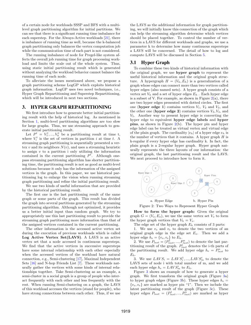
the original graph, we use hyper graph to represent theuseful historical information and the original graph struc-ture. A hypergraph H = (Vh, Eh) is a generalization of agraph whose edges can connect more than two vertices calledhyper edges (also named nets). A hyper graph consists of avertex set Vh and a set of hyper edges Eh . Each hyper edgeis a subset of V. For example, as shown in Figure 2(a), thereare two hyper edges presented with dotted circles. The firstone (hyper edge 1) contains vertices V1, V2 and V3, andthe other one (hyper edge 2) contains vertices V3, V4, andV5. Another way to present hyper edge is converting thehyper edge to equivalent hyper edge labels and hyperpins, as shown in Figure 2(b). The hyper pin and hyperedge label can be treated as virtual vertex and virtual edgeof the plain graph. The cardinality |eh| of a hyper edge eh isthe number of vertices that it contains. A hyper graph H isk-regular if every hyper edge has cardinality k. In fact, theplain graph is a 2-regular hyper graph. Hyper graph nat-urally represents the three layouts of our information: theoriginal graph, the last partitioning result and the LAVS.We next proceed to introduce how to form it.

1

2

34

5

Hyper Edge 1

Hyper Edge 2

a. Hyper Edge

1

2

34

5

Hyper Pins

1

2

b. Hyper Pin

Figure 2: Two Ways to Represent Hyper Graph

How to form the hyper graph: Given the originalgraph G = (Vo, Eo), we use the same vertex set Vo to formthe hyper graph vertices that Vh = Vo.

The edge set of the hyper graph Eh consists of 3 parts:1. We use vs and ve to denote the two vertices of an

original graph edge in the edge set Eo. Then we add ahyper edge he = {vs, ve} to Eh.

2. We use Plast = (P 1last, ..., P

nlast) to denote the last par-

titioning result of the graph. P ilast denotes the i-th parts of

the partitioning result. We add hyper edge he = Pnlast to

Eh.3. We use LAV Si = LAV S1

i , ..., LAV Sim to denote the

LAVS sets of node i with total number of m, and we addeach hyper edge he = LAV Si

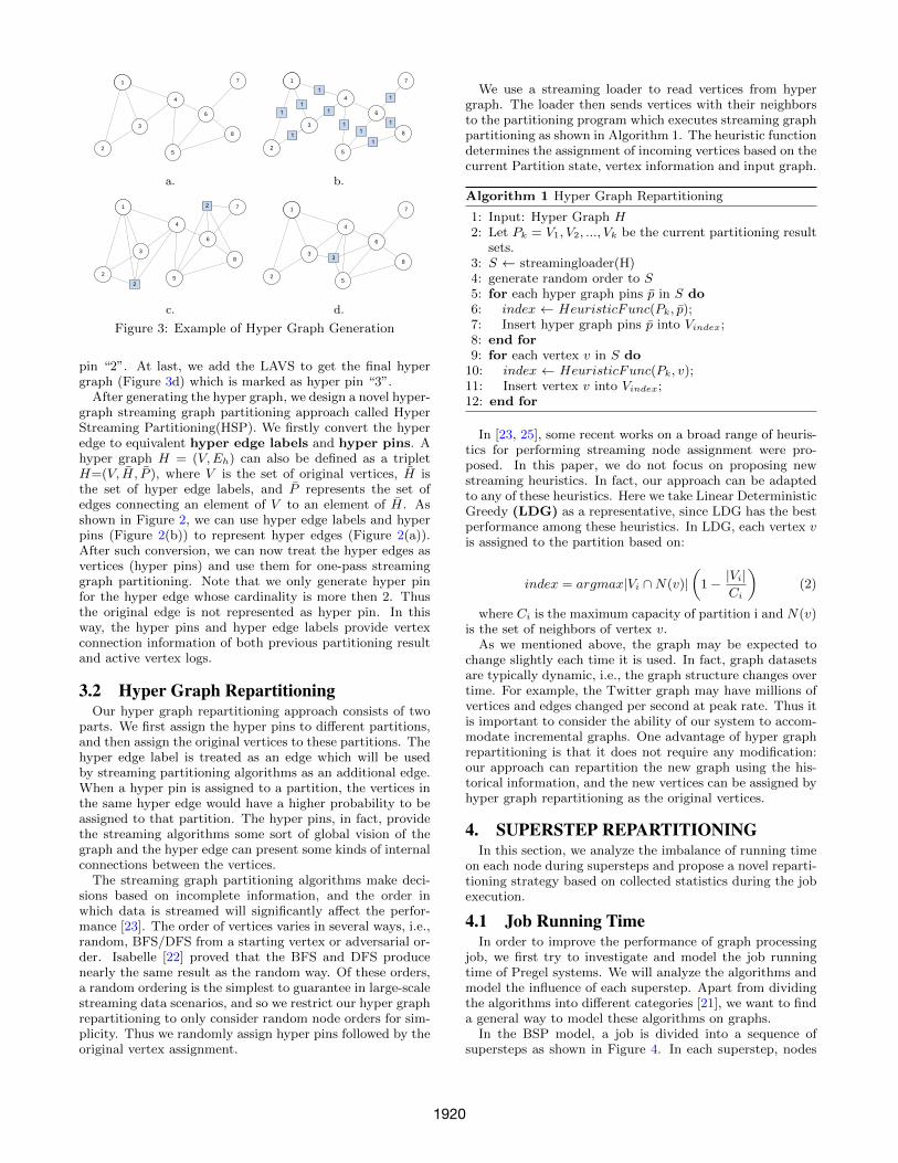
m to Eh.Figure 3 shows an example of how to generate a hyper

graph. We first transform the original graph (Figure 3a)to hyper graph edges (Figure 3b). These hyper edges he ={vs, ve} are marked as hyper pin “1”. Then we include thelatest partitioning result of the graph (Figure 3c). Thesehyper edges Plast = (P 1

last, ..., Pnlast) are marked as hyper

1919

11

2

3

4

5

6

7

8

a.

11

2

3

4

5

6

7

8

1

1

1

1

1

1

1

1

1

1

b.

2

11

2

3

4

5

6

7

8

2

c.

3

11

2

3

4

5

6

7

8

d.

Figure 3: Example of Hyper Graph Generation

pin “2”. At last, we add the LAVS to get the final hypergraph (Figure 3d) which is marked as hyper pin “3”.

After generating the hyper graph, we design a novel hyper-graph streaming graph partitioning approach called HyperStreaming Partitioning(HSP). We firstly convert the hyperedge to equivalent hyper edge labels and hyper pins. Ahyper graph H = (V,Eh) can also be defined as a tripletH=(V, H, P ), where V is the set of original vertices, H isthe set of hyper edge labels, and P represents the set ofedges connecting an element of V to an element of H. Asshown in Figure 2, we can use hyper edge labels and hyperpins (Figure 2(b)) to represent hyper edges (Figure 2(a)).After such conversion, we can now treat the hyper edges asvertices (hyper pins) and use them for one-pass streaminggraph partitioning. Note that we only generate hyper pinfor the hyper edge whose cardinality is more then 2. Thusthe original edge is not represented as hyper pin. In thisway, the hyper pins and hyper edge labels provide vertexconnection information of both previous partitioning resultand active vertex logs.

3.2 Hyper Graph RepartitioningOur hyper graph repartitioning approach consists of two

parts. We first assign the hyper pins to different partitions,and then assign the original vertices to these partitions. Thehyper edge label is treated as an edge which will be usedby streaming partitioning algorithms as an additional edge.When a hyper pin is assigned to a partition, the vertices inthe same hyper edge would have a higher probability to beassigned to that partition. The hyper pins, in fact, providethe streaming algorithms some sort of global vision of thegraph and the hyper edge can present some kinds of internalconnections between the vertices.

The streaming graph partitioning algorithms make deci-sions based on incomplete information, and the order inwhich data is streamed will significantly affect the perfor-mance [23]. The order of vertices varies in several ways, i.e.,random, BFS/DFS from a starting vertex or adversarial or-der. Isabelle [22] proved that the BFS and DFS producenearly the same result as the random way. Of these orders,a random ordering is the simplest to guarantee in large-scalestreaming data scenarios, and so we restrict our hyper graphrepartitioning to only consider random node orders for sim-plicity. Thus we randomly assign hyper pins followed by theoriginal vertex assignment.

We use a streaming loader to read vertices from hypergraph. The loader then sends vertices with their neighborsto the partitioning program which executes streaming graphpartitioning as shown in Algorithm 1. The heuristic functiondetermines the assignment of incoming vertices based on thecurrent Partition state, vertex information and input graph.

Algorithm 1 Hyper Graph Repartitioning

1: Input: Hyper Graph H2: Let Pk = V1, V2, ..., Vk be the current partitioning result

sets.3: S ← streamingloader(H)4: generate random order to S5: for each hyper graph pins p in S do6: index ← HeuristicFunc(Pk, p);7: Insert hyper graph pins p into Vindex;8: end for9: for each vertex v in S do

10: index ← HeuristicFunc(Pk, v);11: Insert vertex v into Vindex;12: end for

In [23, 25], some recent works on a broad range of heuris-tics for performing streaming node assignment were pro-posed. In this paper, we do not focus on proposing newstreaming heuristics. In fact, our approach can be adaptedto any of these heuristics. Here we take Linear DeterministicGreedy (LDG) as a representative, since LDG has the bestperformance among these heuristics. In LDG, each vertex vis assigned to the partition based on:

index = argmax|Vi ∩N(v)|(

1− |Vi|Ci

)(2)

where Ci is the maximum capacity of partition i and N(v)is the set of neighbors of vertex v.

As we mentioned above, the graph may be expected tochange slightly each time it is used. In fact, graph datasetsare typically dynamic, i.e., the graph structure changes overtime. For example, the Twitter graph may have millions ofvertices and edges changed per second at peak rate. Thus itis important to consider the ability of our system to accom-modate incremental graphs. One advantage of hyper graphrepartitioning is that it does not require any modification:our approach can repartition the new graph using the his-torical information, and the new vertices can be assigned byhyper graph repartitioning as the original vertices.

4. SUPERSTEP REPARTITIONINGIn this section, we analyze the imbalance of running time

on each node during supersteps and propose a novel reparti-tioning strategy based on collected statistics during the jobexecution.

4.1 Job Running TimeIn order to improve the performance of graph processing

job, we first try to investigate and model the job runningtime of Pregel systems. We will analyze the algorithms andmodel the influence of each superstep. Apart from dividingthe algorithms into different categories [21], we want to finda general way to model these algorithms on graphs.

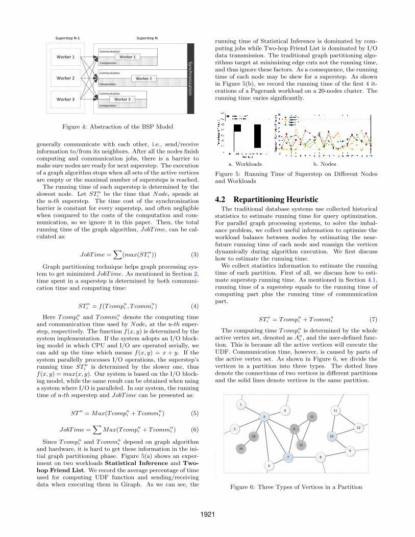
In the BSP model, a job is divided into a sequence ofsupersteps as shown in Figure 4. In each superstep, nodes

1920

Worker 1

Superstep NSuperstep N-1

Worker 1

Worker 2

Worker 3

Synchronization

Computation

Worker 2

Worker 3

Communication

Computation

Communication

Computation

Communication

Figure 4: Abstraction of the BSP Model

generally communicate with each other, i.e., send/receiveinformation to/from its neighbors. After all the nodes finishcomputing and communication jobs, there is a barrier tomake sure nodes are ready for next superstep. The executionof a graph algorithm stops when all sets of the active verticesare empty or the maximal number of supersteps is reached.

The running time of each superstep is determined by theslowest node. Let STn

i be the time that Nodei spends atthe n-th superstep. The time cost of the synchronizationbarrier is constant for every superstep, and often negligiblewhen compared to the costs of the computation and com-munication, so we ignore it in this paper. Then, the totalrunning time of the graph algorithm, JobT ime, can be cal-culated as:

JobT ime =∑

(max(STni )) (3)

Graph partitioning technique helps graph processing sys-tem to get minimized JobT ime. As mentioned in Section 2,time spent in a superstep is determined by both communi-cation time and computing time:

STni = f(Tcompni , T comm

ni ) (4)

Here Tcompni and Tcommni denote the computing time

and communication time used by Nodei at the n-th super-step, respectively. The function f(x, y) is determined by thesystem implementation. If the system adopts an I/O block-ing model in which CPU and I/O are operated serially, wecan add up the time which means f(x, y) = x + y. If thesystem parallelly processes I/O operations, the superstep’srunning time STn

i is determined by the slower one, thusf(x, y) = max(x, y). Our system is based on the I/O block-ing model, while the same result can be obtained when usinga system where I/O is paralleled. In our system, the runningtime of n-th superstep and JobT ime can be presented as:

STn = Max(Tcompni + Tcommni ) (5)

JobT ime =∑

Max(Tcompni + Tcommni ) (6)

Since Tcompni and Tcommni depend on graph algorithm

and hardware, it is hard to get these information in the ini-tial graph partitioning phase. Figure 5(a) shows an exper-iment on two workloads Statistical Inference and Two-hop Friend List. We record the average percentage of timeused for computing UDF function and sending/receivingdata when executing them in Giraph. As we can see, the

running time of Statistical Inference is dominated by com-puting jobs while Two-hop Friend List is dominated by I/Odata transmission. The traditional graph partitioning algo-rithms target at minimizing edge cuts not the running time,and thus ignore these factors. As a consequence, the runningtime of each node may be skew for a superstep. As shownin Figure 5(b), we record the running time of the first 4 it-erations of a Pagerank workload on a 20-nodes cluster. Therunning time varies significantly.

a. Workloads b. Nodes

Figure 5: Running Time of Superstep on Different Nodesand Workloads

4.2 Repartitioning HeuristicThe traditional database systems use collected historical

statistics to estimate running time for query optimization.For parallel graph processing systems, to solve the imbal-ance problem, we collect useful information to optimize theworkload balance between nodes by estimating the near-future running time of each node and reassign the verticesdynamically during algorithm execution. We first discusshow to estimate the running time.

We collect statistics information to estimate the runningtime of each partition. First of all, we discuss how to esti-mate superstep running time. As mentioned in Section 4.1,running time of a superstep equals to the running time ofcomputing part plus the running time of communicationpart.

STni = Tcompni + Tcommn

i (7)

The computing time Tcompni is determined by the wholeactive vertex set, denoted as An

i , and the user-defined func-tion. This is because all the active vertices will execute theUDF. Communication time, however, is caused by parts ofthe active vertex set. As shown in Figure 6, we divide thevertices in a partition into three types. The dotted linesdenote the connections of two vertices in different partitionsand the solid lines denote vertices in the same partition.

2

1

3

4

6

7 8

10

12

9

11

5

11

13

1214

Figure 6: Three Types of Vertices in a Partition

1921

Type1: Vertices and their neighbors are adjacent to ver-tices in the same partition. For example, vertices 5, 11, 12,13 and 14 are of this type. We use αn

i to denote the verticesbelonging to this type in n-th superstep on nodei.Type2: Vertices that are adjacent to vertices from other

partition. For example, vertices 1, 2 and 4 are of this type.We use βn

i to denote the vertices belonging to this type inn-th superstep on nodei.Type3: Vertices that are adjacent to only vertices in the

same partition while their neighbors are adjacent to verticesfrom other partitions. We use γn

i to denote the vertices be-longing to this type in n-th superstep on nodei. The vertices3, 7 and 10 belong to this type.

The first type vertices generate only local messages. Inparallel graph processing system, producing and processinglocal messages are extremely faster than non-local messages,so we ignore the time cost for dealing with local messages.Thus vertices in Type1 do not generate communication time.

The second type vertices send and receive messages fromtheir adjacent partition(s). The total communication timein this superstep is caused by this subset of active vertices.We can now denote the superstep running time as:

STni = tComp ∗ |An

i |+ tComm ∗ |βni | (8)

tComp and tComm are the average computing time andcommunication time used by each vertex. LogGP uses run-ning logs to get these two parameters during the job execu-tion. Detailed information will be discussed in Section 5.

As same as Type1, the vertices of Type3 do not generatecommunication cost, because there is no non-local verticesadjacent to it. However, these vertices may activate the ver-tices of Type2 to generate communication cost in the nextsuperstep. Thus we can use these vertices of Type3 to esti-mate the communication time in the next superstep.

Another problem is that how can we get the number ofvertex set βn+1

i with the information of γni . Here we in-

troduce a new metric, active ratio, denoted as λ. Activeratio denotes the probability of an active vertex v in super-step N that causes the neighbors of that vertex to be activein superstep N + 1. For example, the active ratio of algo-rithm Pagerank is always 100% because the active vertexwill always activate its neighbors in next superstep. Theseparameters can be obtained by the historical log as well.

Then, we can calculate |βn+1i | and |An+1

i | with λ:

|βn+1i | = |γn

i | ∗ λ (9)

|An+1i | = |An

i | ∗ λ (10)

The running time of (n+1)-th superstep can be estimated:

STn+1i = (tComp ∗ |An

i |+ tComm ∗ |γni |) ∗ λ (11)

After estimating the running time of the next superstep,we collect the estimated running time of each node, andreassign the vertices to rebalance the running time of thenext superstep.

However, vertex reassignment (repartitioning) is still dif-ficult because:

1) Finding the optimal repartitioning is an NP problem, asthe size-balanced graph partition problem is NP-complete [6]which is the static setting of our problem.

2) The computational overhead from the repartitioningcost must be low. As the objective is to improve application

performance, the selected technique must be lightweight andcan be scalable to work on large graphs.

3) Synchronizing distributed states of different partitionsdynamically is impossible. Propagating global informationacross the network incurs a significant overhead, which mustbe considered for our repartitioning technique. Thus therepartitioning approach can only use a local view of thegraph.

The basic idea is to reassign the vertex from partitionswith long estimated time to short ones before the next su-perstep. We use a threshold θn+1 to determine whether theestimated time is long in the total running time.

θn+1 = ϑ ∗∑STn+1

i

i(12)

Here ϑ is the percentage which we will discuss below. Wemove vertices from the partitions that STn+1

i are larger thanθn+1 to the other partitions and try to minimize the longestrunning time.

In this paper, we propose a novel heuristic that movesthe vertex which will generate communication cost in thenext superstep to an appropriate partition. The movementwill reduce the total communication cost in the future andbalance the running time of each node in next superstep.For a vertex vi in nodei, LogGP logs the times of the vertexcommunicating to other partitions and denotes it as C(vi).If a vertex repartitioning is needed on nodei, we first choosethe vertices that may generate remote communication inthe next n+1 superstep, denoted as Γi

n+1. Let N(v) be theneighbor set of vertex v.

Γin+1 =

⋂N(v), v ∈ γn

i (13)

We then sort the remote communication times, C(vi), foreach of the vertex in Γi

n+1 in a non-descending order andgreedily reassign the vertex with the max C(Vt) to the par-tition that the vertex has the most neighbors. When a vertexis removed, the estimated running time will be decreased bytComp + tComm. The reassignment stops when Γi

n+1 isempty or the estimated running time of the next superstepis equal to the average. The whole processing is illustratedin Algorithm 2.

Algorithm 2 Superstep Repartitioning

1: STn+1i ← estimated running time of N + 1 superstep

2: if STn+1i > ϑ ∗

∑STn+1

ii

then

3: Γin+1 ←

⋂N(v), v ∈ γn

i //N(v) is the neighbor vertexset of v

4: List ← C(v), v ∈ Γin+1 //List records the C(v) of

vertex in Γin+1

5: List ← Sort List in non-descending order

6: while Γin+1 6= ∅ and STn+1

i <∑

STn+1i

mdo

7: // m is the number of partitions8: vt ← pop(List)9: Reassign vt to the partition that the vt has the most

neighbors10: Γi

n+1 ← Γin+1 − (tComp+ tComm)

11: end while12: end if

1922

5. THE LogGP ARCHITECTUREIn this section, we present an overview of LogGP to show

how the proposed techniques can be seamlessly integratedinto the system to improve the performance. We first pro-vide the system architecture, and then present the key com-ponents of the system. Finally, we discuss how we managethe vertex migration.

System Architecture: We first describe the basic ar-chitecture and operations of LogGP. Figure 7 depicts howLogGP is integrated into Giraph (open source version ofPregel) as a middle-ware. Our system can be easily mi-grated to any other BSP-based graph processing systems aswell. In the Giraph system, there are two types of process-ing nodes: master node and worker node. There is onlyone master node which manages to assign and coordinatejobs, and there are multiple worker nodes which executeuser defined function against each vertex assigned to them.The components of LogGP are running on the correspond-ing nodes of Giraph nodes. There is a LogGP partitioningmanager (PM) running on the master node that providespartitioning meta data for the master node. A LogGP par-titioning agency (PA) is running on each of the worker nodesto record, collect and report log information of that workernode to PM. The initial graph data is partitioned on PMand assigned to each worker.

PartitioningManager

Master Node

WorkerNode #1

WorkerNode #2

WorkerNode #3

WorkerNode #4

Partitioning Agency

Partitioning Agency

Partitioning Agency

...

Partitioning Agency

Hadoop Distributed File System (HDFS)

LogGPMiddle-ware

Figure 7: Architecture of LogGP Integrated on Giraph

Both PM and PA share the communication frameworkof Giraph to communicate with each other. The persistentdata, such as historical partitioning result, is stored in theHDFS [4] shared with Giraph as well. The detailed discus-sion of the key components is as follows:

LogGP Partitioning Manager: Partitioning Manager(PM) is a process running on the master node. It storesthe meta data of graphs and historical partitioning results.There is a unique GraphID for each graph in LogGP , whichrepresents a certain graph. The meta data stores the link ofthe graph’s historical information, such as the latest parti-tioning result or the LAVS of that graph. The actual data isstored on HDFS and PM can access that file by the link ofmeta data. When a job is to run on a graph, the master nodewill ask PM to generate the Hyper Graph with the originalgraph, if existed, the latest partitioning result and LAVSof the that graph. After that, PM partitions the graph togenerate the initial partitioning. Then, PM checks the metadata and fetches the historical information to generate theinitial partitioning result for this graph. The master node

then uses this partitioning result to assign vertices of thegraph from HDFS to worker nodes.

During the job execution, when each worker finishes asuperstep, it sends the estimated running time of that par-tition to PM. PM then gathers and analyzes the informationfrom worker nodes and applies the repartitioning strategy tooptimize the running time of the next superstep. If a repar-titioning is needed for a partition on a node, PM will send arepartitioning trigger along with the necessary informationto the PA of that node and a repartitioning procedure willbe started on that node.

LogGP Partitioning Agency: Partitioning Agency (PA)is running on each worker node in the Giraph system to col-lect running time information and manage to repartition thegraph when there will be a running time skew in the next su-perstep. PA uses the same communication module in Giraphto communicate with PM or other PA(s). PA collects theinformation when the superstep is running, such as tComp,tComm and C(v), then uses this information to computethe estimated running time for the next superstep. In fact,when a vertex is executing a user defined function, such asPagerank, PA will check the type of vertex and record thetime used for computing. When data is sent to the otherpartitions, PA records the vertex sets and the time spenton the communication. This running log will be analyzedafter each superstep finishes and generates statistical logsfor that superstep. tComp, tComm, C(v) and other param-eters used for superstep repartitioning are obtained fromthese logs. When a superstep is finished, in synchronizationstep, PA will send the estimated time of next superstep toPM and wait for the response from PM. If a repartition isnecessary, PM will run the repartitioning heuristic to rebal-ance the running time. PA also writes running logs of activesets of each superstep. When the workload is finished, LAVSis generated from the running logs. When all the LAVSs ofcontinuous k supersteps are generated, the results are up-loaded to HDFS for PM to generate Hyper Graph for nextworkload. This process is fast and does not take much re-source in that node.

Vertex Migration: For Superstep Repartitioning, whenthe dynamic partitioning scheme decides to reassign verticesfrom one partition to another, three types of data need tobe sent: (1) latest value of vertices; (2) adjacency list ofvertices; (3) messages for the next superstep. One solutionis to add a new stage for vertex reassign between the end ofsuperstep n and beginning of superstep n+1. LogGP usesanother option that combines vertex moving within the Syn-chronization stage. We combine the messages sent from onepartition to another to reduce the times of communication.In addition, the number of vertexes which need to be movedis small. Thus, the reassignment cost is slight compared withother operations. We will further discuss the time used forvertexes reassignment in experiment studies.

When a vertex gets reassigned to a new worker, everyworker in the cluster must obtain and store this informationin order to deliver future messages to the vertex. An obviousoption for each worker is to store an in-memory map consist-ing of < V ertexid,Workerid > pairs. However, using thissolution, a vertex u must broadcast to all its neighbors whenit is moved from one node to another. To reduce the cost, weimplement an high-efficient lookup table service mentionedin [24] to provide a lookup table that reduces the broadcastcost when reassigning vertices.

1923

6. EVALUATIONIn this section, we evaluate the performance of our pro-

posed partitioning refinement approaches. We implementedLogGP on Giraph [1], and the lookup table service [24] forvertex migration solution.

6.1 Experimental SettingsWe first briefly introduce the experimental settings for the

evaluation, including datasets, evaluation metrics and com-parative approaches. All the experiments were conducted ona cluster with 28 nodes with an AMD Opteron 4180 2.6GhzCPU, 48GB memory and a 10TB RAID disk. All the nodeswere connected by 1Gbt bandwidth routers.

6.1.1 Data SetsWe used 5 real-world datasets: Live-Journal, Wiki-Pedia,

Wiki-Talk, Twitter and Web-Google; and one Synthetic graphwhich is generated following the Erdos-Renyi random graphmodel. Those real-world datasets are publicly available onthe Web [5], and the statistics of the datasets are shownin Table 1. We transformed them into undirected graphs,added reciprocal edges and eliminated loop circles from theoriginal release.

Dataset Nodes Edges Type SizeWiki-pedia 2,935,762 35,046,792 Web 401MBWiki-Talk 2,388,953 4,656,682 Web 64MB

Web-Google 875,713 8,644,106 Web 72MBLive-Journal 4,843,953 42,845,684 Socia 479MB

Twitter 41,652,230 1,468,365,182 Social 20GBSynthetic 5,000,000 100,000,000 Synthetic 930MB

Table 1: Graph Dataset Statistics

6.1.2 Evaluation MetricsWe use two metrics to systematically evaluate the result

of our experiment. For both of the two metrics, a lowervalue represents the better performance.

Edge Cut Percentage(ECP): It indicates the percentage ofcut edges between partitions in the graph, defined as ECP =ec/|E|, where ec denotes the number of cut edges betweenpartitions, and |E| denotes the total number of edges in thegraph. This is the basic metric to evaluate the quality ofpartitioning result.

Execution Time: We utilize two time costs to evaluate thesystem performance. The first one is Job Execution Time(JET) which presents the elapsed time from submitting agraph workload till its completion. We use JET to eval-uate the actual effectiveness of the partitioning. After wepartition the graph, we run the workload on the partitionedgraph and record the time. The second one is Total RunningTime which includes the workload execution time, as wellas the graph loading and partitioning time.

6.1.3 Comparative MethodsIn this experimental study, we select several state-of-the-

art partitioning methods for comparison to demonstrate theadvantage of our proposed method.

• The proposed LogGP method uses two techniques,Hyper Graph Repartitioning (HGR) and Superstep

Repartitioning (SR), to reduce the overall job execu-tion time of graph system. To better examine the ef-fectiveness of our approach, we also study the perfor-mance of HGR and SR individually.

• Linear Deterministic Greedy (LDG) approach [23] isconsidered as one of best static streaming method, andRestreaming LDG (reLDG) approach [19] is extendedto generate initial graph partitioning using the laststreaming partitioning result.

• CatchW [21] is a dynamic graph workload balancingapproach for random initial partitioning, which is acomparative approach for SR, as both of them try toadjust the partitions in the supersteps.

• We also use Hashing as one competitor because ofits simplicity and popularity, e.g., Pregel uses hashfunction to partition the vertices by default.

6.2 Effect of Hyper Graph RepartitioningWe first evaluate the performance of Hyper Graph Repar-

titioning (HGR). The state-of-the-art streaming algorithmLDG [23], reLDG [19] and Hashing are used as the baseline. We run the experiment against all the graph datasetsshown in Table 1. Here we mainly present the results onLive-Journal, Web-Google and Synthetic dataset as repre-sentative of Social Graph, Web Graph and Random Graphrespectively.

Figure 8 shows the ECP of partitioning results on thesethree types of datasets. Each partitioning algorithm is ex-ecuted 10 times, and HGR and reLDG use the last parti-tioning result for repartitioning. To generate the LAVS forthe hyper graph, we execute a Semi-clustering workload af-ter the partitioning. As we can see, HGR works well on allthe graphs, especially on the Social Graph. This is mainlybecause that these social graphs representing real relation-ships of social network have significantly higher average lo-cal clustering coefficient. After running the Semi-clusteringworkload, LogGP records the LAVS of Semi-clustering thatrepresent the internal relationships of these vertices. ThenHGR generates Hyper Graph with this additional informa-tion to repartition the graph. With the help of Hyper Graph,streaming algorithm HGR can use more useful vertex rela-tion to get better partitioning result. Thus, our approachoutperforms reLDG which only uses the partitioning resultwhile our approach uses additional LAVS information forinitial partition. For Web Graph, known as seriously power-law skewed, our approach is still the best. Though in Syn-thetic Random Graph, our approach gets the smallest im-provement, there is still about 15% reduction of ECP com-paring with LDG. For Random Graph, there is no internalconnection between vertices, thus, LAVS cannot fetch therelationships resulting in less improvement. However theprevious partitioning result is shown to be helpful for theserandom graph as well.

In addition, we evaluate the running time of these par-titioning results after 10 times repartitioning. We run a10-iteration of Pagerank and Semi-Clustering workloads onLive-Journal dataset. We compare the running time of HGRwith Hashing, reLDG and LDG. As shown in Figure 9(a),HGR significantly reduces the running time on these twoworkloads, which confirms that our approach can refine thestreaming partitioning result with the Hyper Graph.

1924

a. ECP Results of 10 Iterations on Live-Journal

b. ECP Results of 10 Iterations on Web-Google

c. ECP Results of 10 Iterations on Random Graph

Figure 8: ECP of 10 Iterations on 3 Types of Datasets

In real-world, the workload and graphs are changing timeby time. To simulate the graph changing, we evaluate ourmethod using graph that changes dynamically between dif-ferent workload iterations. We used 75% vertices in thegraph for the first workload and then added 5% verticeseach time. At last, when the workload is running for the5 times, all the vertices is used. We evaluate the runningtime of HGR compared with other partitioning algorithmsafter 5 times repartitioning, and the results shown in Fig-ure 9(b) demonstrate the efficiency and robustness of ourapproach with respect to graph updates. We also designan experiment to evaluate the situation when workload ischanging during different iterations. We use 5 workloads:Semi-Clustering, Two-hop Friendship, Single Source Short-est Path, Breadth First Search and Pagerank for workload1, 2, 3, 4 and 5 iterations separately. We execute these 5workloads in sequence with HGR and other partitioning al-gorithms, and present the result of the last workload Pager-ank in the paper. Figure 9(b) reports the superiority of ourmethod.

Parameter tunning of HGR: As we mentioned in Sec-tion 3, we use a parameter k to determine the size of verticesin a LAVS. We conduct a series of experiments to investi-gate the selection of k. Due to the space limit, we only showthe result of ECP on Live-Journal dataset using Pagerank

Semi-Clustering Pagerank

Exe

cutio

n T

ime

(s)

0

100

200

300

400LDGreLDGHGRHashing

a.

Dynamic Graph Mixed Workload

Exe

cutio

n T

ime

(s)

0

100

200

300

400LDGreLDGHGRHashing

b.

Figure 9: Job Execution Time on Live-Journal Dataset

for LAVS, in Figure 10. We find that when k = 2 or k = 3,HGR achieves the best performance for most of the work-loads. This is because when k is small (k = 1), the sizeof LAVS is too small to present the connections betweenvertices. When the size of LAVS becomes larger (k > 3),the LAVS contains too much vertices which may not havestrong relationships. Thus we use k = 3 as the number ofsupersteps to form LAVS in the experiment.

0 1 2 3 4 5 6 7 8 9 10

Edg

e C

ut P

erce

ntag

e

20

30

40

50

60Parameter K

Figure 10: Parameter of LAVS Tuning

6.3 Effect of Superstep RepartitioningWe next present the performance of Superstep Reparti-

tioning (SR). We use a representative communication-intensiveworkload, Pagerank, for the evaluation. The parameter ϑused for the percentage number that determines the thresh-old in Formula 12 is set as 2% which shows better resultthan other values. For Superstep Repartitioning which bal-ances the running time of each partition during the execu-tion, JET is a more important performance metric thanECP. Notice that the JET of SR contains the time of vertexreassignment.

To better understand how Superstep Repartitioning bal-ances the running time of each workload, we show the timeof a sample node on Live-Journal dataset in the first itera-tion of Pagerank workload in Figure 11(a) and the runningtime of the same node in the 4th superstep in Figure 11(b).We can observe that after three times of vertex refinement,the running time of each node is balanced with even shorterrunning time as well. In our experiment, the JET containsthe repartitioning time which is marked as grey bars in Fig-ure 11(b). These results also confirm the efficiency of mi-grating and locating the reassigned vertices in LogGP .

We next evaluate the effect of SR with different datasets.Figure 12(a) shows the result of JET of a 10-iteration Pager-ank workload on different graphs using LDG streaming par-titioning as the initial partitioning. Note that, the initialpartitioning method is orthogonal to superstep repartition-ing, and we will next show results on different initial par-titioning results. We compare SR with CatchW discussedin [21] which is a dynamic graph workload balancing ap-proach. The original method denotes running the experi-

1925

a. Execution Time of 1st Superstep

1 2 3 4 5 6 7 8 9 10 11 12 13 14 15 16 17 18 19 20

Sup

erst

ep E

xecu

tion

Tim

e (s

)

0

10

20

30

40

b. Execution Time of 4th Superstep

Figure 11: JET of One Sample Node in Different Supersteps

ment without repartitioning approach during supersteps. Aswe can see, there is a significant decrease on JET compar-ing with the approaches without Superstep Repartitioning,with a reduction of 11.9% to 27% JET on these datasets.SR runs faster than CatchW on all of the 3 datasets.

a. Performance of Pagerank b. Comparing with CatchW

Figure 12: Performance of Superstep Repartitioning

We further evaluate the influence of different initial par-tition results to SR. We use the results of HGR, LDG andHashing approaches as initial partition results. Figure 12(b)summarizes the JET cost of these three repartitioning ap-proaches. We run the experiment on Live-Journal datasetfor 10-iteration Pagerank workload. As shown in Figure 12(b),our repartitioning approach yields impressive performanceon HGR and LDG while there is no significant improvementon Hashing initial partition. The reason is that our algo-rithm focuses on balancing the execution time of each nodeduring superstep. The hashing partition is actually morebalanced, although running slower, than LDG. For LDG asinitial partition, our approach outperforms CatchW, whileCatchW is better on LiveJournal dataset with Hashing asinitial partitioning. CatchW is primarily designed for start-ing from an initial random graph partitioning and reassign-ing the vertices to reduce the communication cost, whileour approach focuses on how to balance the running timeof each node according to the running log from a streaminginitial partitioning. Clearly, our approach is more efficientfor practical situation.

This experiment indicates our Superstep Repartitioningapproach can balance the running time during executionand reduce the total execution time of graph processing job.

6.4 The Superiority of LogGPFrom the previous experiments, we can see that Hyper

Graph Repartitioning (HGR) and Superstep Repartition-ing (SR) yield promising results in initial graph partition-ing and superstep graph adjustment respectively. In this ex-periment, we investigate the overall performance of LogGPwhich can take the both advantages of HGR and SR.

Figure 13: Overall Performance of logGP

Figure 13 illustrates the Running time of 10-iteration Pager-ank and Semi-clustering workload on Twitter dataset. Wecompare with all the approaches mentioned above: LDG,reLDG, and CatchW. As we can observe, comparing to LDG,there are about 49.1% running time reduction on Semi-clustering and 39.2% improvement on Pagerank. The re-sult of LogGP outperforms the CatchW and reLDG as well.These results confirm that LogGP with the help of log infor-mation can significantly reduce the job execution time whencomparing with other approaches.

Maximal Independent Sets Two-hop Friendship

Exe

cutio

n T

ime

(s)

0

100

200

300

400

500LDGreLDGLogGPCatchWHashing

a. Wiki-Pedia

Maximal Independent Sets Two-hop Friendship

Exe

cutio

n T

ime

(s)

0

50

100

150

200

250

300LDGreLDGLogGPCatchWHashing

b. Wiki-Talk

Figure 14: Performance on Other Datasets

Besides Twitter dataset, we also evaluate the systems onWiki-Pedia and Wiki-Talk dataset with workloads Maximal

1926

Independent Sets and Two-hop Friendship. As shown inFigure 14, LogGP outperforms all the other methods onall these datasets and workloads. These results here alsoreveal the generality of the proposed approach and its wideapplication to various domains.

We next conduct the experiments to further study the to-tal runing time of the graph processing job. We run thePagerank 10-iteration workload on Live-Journal data, andFigure 15 shows the results of total running time includ-ing graph loading time (grey bar), partitioning time (whitebar), and JET (black bar). The overall performance of ourmethod is the best, though it introduces slightly more par-titioning overhead.

LDG reLDG LogGP CatchW Hashing

Tot

al R

unni

ng T

ime

(s)

0

100

200

300

400

JETGraph LoadingPartitioning

Figure 15: Study of Total Running Time

Number of Workers

10 20 30 40 50 60 70 80 90 100

Exe

cutio

n T

ime

(s)

0

100

200

300

400

500LogGPIdeal

a. Different Workers

Number of Nodes

1 2 3 5 10 15 20 25

Exe

cutio

n T

ime

(s)

0

200

400

600

LogGP

b. Different Nodes

Figure 16: Performance of Scalability

Scalability Study: Scalability is an important featurefor parallel graph processing system. We further evaluatedthe scalability of LogGP with 1) fixed number of 28 nodescluster and increasing number of workers; 2) fixed numberof 100 workers and increasing number of nodes.

Figure 16(a) shows the performance of running 50-iterationof Pagerank on the Live-Journal with the number of workersincreasing from 10 to 100. We use an ideal curve to denotethe ideal execution time which assumes the performance islinear to the worker number for comparison. As expected, asthe number of workers increases, the improvement decreasesslightly and the performance of LogGP is close to the ideal.This result confirms that LogGP has a graceful scalability.

We also conduct an experiment by varying the number ofnodes from 1 to 25 with fixed 100 workers, and the results areshown in Figure 16(b). Not surprisingly, the performance onone node outperforms that of two and three nodes, becausethe cluster with multiple nodes introduce extra communica-tion cost between nodes. However, it is clear that LogGPperforms better if we further increase the number of nodes,e.g., ≥ 5, as the gain from the computation capacity of clus-ter overcomes the communication overhead.

To summarize, based on our experimental results, we con-clude that LogGP can take advantage of historical log infor-mation for partitioning refinement and provide an effectivepartitioning solution for large graph processing system.

7. RELATED WORKThe graph partition problem discussed in this paper is

related to several fields such as graph computing systemsand graph partitioning.

Large-Scale Graph Computing: To meet the currentprohibitive requirements of processing large-scale graphs,many distributed methods and frameworks have been pro-posed and become appealing. Pregel [17] and GraphLab [15]both use a vertex-centric computing model, and run a userdefined program at each worker node in parallel. Hama [2]and Giraph [1] are open source projects, which adopt Pregelprogramming model, and adjust for HDFS. In these par-allel graph processing systems, it is important to partitionlarge graph into several balanced sub-graphs, so that paral-lel workers can coordinately process them. However, mostof the current systems usually choose simple hash method.

Graph partitioning: Graph partitioning is a combi-natorial optimization problem which has been studied fordecades. The k-balanced graph partitioning aims to mini-mize the number of edge cut between partitions while bal-ance the number of vertices. Though the k-balanced graphpartitioning problem is an NP-Complete problem [10], sev-eral solutions have been proposed to tackle this challenge.

Andreev et al. [6] presented an approximation algorithmwhich guarantees polynomial running time with an approxi-mation ratio of O(logn). Another solution was proposed byEven et al. [9] who gave an LP solution based on spreadingmetrics which also gets an O(logn) approximation. Besidesapproximated solution, Karypis et al. [14] proposed a par-allel multi-level graph partitioning algorithm to minimizebisection on each level. There are some heuristics imple-mentations like METIS [13], parallel version of METIS [20]and Chaco [12] which are widely used in many existing sys-tems. Although they cannot provide precise performanceguarantee, these heuristics are quite effective. More heuris-tic approaches were summarized in [3].

The methods mentioned above are offline and require longprocessing time generally. Recently, Stanton and Kliot [23]proposed a series of online streaming partitioning methodusing heuristics. Fennel [25] extended this work by propos-ing a streaming partitioning framework which combines otherheuristic methods. Joel Nishimura and Johan Ugander [19]futher proposed Restreaming LDG and Restreaming Fen-nel that generated initial graph partitioning using the laststreaming partitioning result. Restreaming LDG and Re-streaming Fennel exploits the similar strategy as HGR. How-ever, HGR further uses the Log Active Vertex Set to get theinternal relationship between vertices and combines the orig-inal graph, last streaming partitioning result and Log ActiveVertex Set into a Hyper Graph. HGR then uses a novel Hy-per Graph Streaming Repartitioning algorithm to partitionthe graph with global information.

Beyond these static graph partitioning technologies, [18]theoretically studies how to adapt graph structure chang-ing without the overhead of reloading or repartitioning thegraph. Some of the recent works [27, 8] can cope with thechanges in graph structure. However, these approaches han-dle the changing in high cost. Shang et al. [21] investigatedseveral graph algorithms and proposed simple yet effectivepolicies that can achieve dynamic workload balance, whilethis approach uses hashing partitioning as the initial input.Compared to our repartitioning approach SR, CatchW triesto minimize the total communication cost. SR focuses on

1927

reducing the total JET of the systems which is more effec-tive. In addition, SR uses the running statistical informationduring the execution and predicts the running time of eachnode in the next superstep. Base on the prediction, SR canaccurately move the proper vertices.

8. CONCLUSIONIn this paper, we systematically investigated the imbal-

ance of running time on BSP model. We designed a novellog-based graph partitioning system to reuse the previousand running log information for partitioning refinement. Weproposed Hyper Graph Partitioning which combines the graphand historical partitioning results to generate a hyper graphto improve the initial partitioning result. When the work-load is executing, we use the running logs to estimate therunning time of each node and design a novel heuristic toreassign the vertices from skew nodes to balance the run-ning time. Prototype and experimental results confirmedthe improvements of our new approaches.

There are several promising directions for our future work.First, a further theoretical analysis of streaming algorithmfor Hyper Graph is preferred for better cost estimation. Sec-ond, other heuristics for vertex reassignment during the ex-ecution is an interesting topic.

9. ACKNOWLEDGEMENTThe research is supported by the National Natural Science

Foundation of China under Grant No. 61272155 and 973program under No. 2014CB340405.

10. REFERENCES[1] Apache Giraph.

https://github.com/apache/giraph/.

[2] Apache Hama. http://hama.apache.org/.

[3] Graph Archive Dataset.http://staffweb.cms.gre.ac.uk/~wc06/partition/.

[4] HDFS. http://hadoop.apache.org/common/docs/current/hdfs/design.

[5] Snap Dataset.http://snap.stanford.edu/data/index.html.

[6] Konstantin Andreev and Harald Racke. Balancedgraph partitioning. Theor. Comp. Sys., 39(6).

[7] Rishan Chen, Mao Yang, Xuetian Weng, Byron Choi,Bingsheng He, and Xiaoming Li. Improving largegraph processing on partitioned graphs in the cloud.In Proc. of SOCC Conference, pages 1–13, 2012.

[8] Raymond Cheng, Ji Hong, Aapo Kyrola, YoushanMiao, Xuetian Weng, Ming Wu, Fan Yang, LidongZhou, Feng Zhao, and Enhong Chen. Kineograph:taking the pulse of a fast-changing and connectedworld. In Proc. of EuroSys, pages 85–98, 2012.

[9] Guy Even, Joseph (Seffi) Naor, Satish Rao, andBaruch Schieber. Fast approximate graph partitioningalgorithms. SIAM Journal on Computing,28(6):2187–2214, 1999.

[10] Michael R Garey, David S Johnson, and LarryStockmeyer. Some simplified np-complete problems. InProc. of STOC Conference, pages 47–63, 1974.

[11] Joseph E. Gonzalez, Yucheng Low, Haijie Gu, DannyBickson, and Carlos Guestrin. Powergraph:distributed graph-parallel computation on natural

graphs. In Proc. of OSDI Conference, pages 17–30,2012.

[12] Bruce Hendrickson and Robert W Leland. Amulti-level algorithm for partitioning graphs. SC,95:28, 1995.

[13] George Karypis and Vipin Kumar. Multilevel graphpartitioning schemes. In Proc. of ICPP Conference,pages 113–122, 1995.

[14] George Karypis and Vipin Kumar. A parallelalgorithm for multilevel graph partitioning and sparsematrix ordering. Journal of Parallel and DistributedComputing, 48(1):71–95, 1998.

[15] Yucheng Low, Danny Bickson, Joseph Gonzalez,Carlos Guestrin, Aapo Kyrola, and Joseph MHellerstein. Distributed graphlab: a framework formachine learning and data mining in the cloud. Proc.of VLDB Endow., 5(8):716–727, April 2012.

[16] Michael Luby. A simple parallel algorithm for themaximal independent set problem. SIAM journal oncomputing, 15(4):1036–1053, 1986.

[17] Grzegorz Malewicz, Matthew H. Austern, Aart J.CBik, James C. Dehnert, Ilan Horn, Naty Leiser, andGrzegorz Czajkowski. Pregel: a system for large-scalegraph processing. In Proc. of SIGMOD Conference,pages 135–146, 2010.

[18] Vincenzo Nicosia, John Tang, Mirco Musolesi,Giovanni Russo, Cecilia Mascolo, and Vito Latora.Components in time-varying graphs. Chaos: AnInterdisciplinary Journal of Nonlinear Science,22(2):1–12, 2012.

[19] Joel Nishimura and Johan Ugander. Restreaminggraph partitioning: Simple versatile algorithms foradvanced balancing. In Proc. of SIGKDD conference,pages 1106–1114, 2013.

[20] Kirk Schloegel, George Karypis, and Vipin Kumar.Parallel static and dynamic multi-constraint graphpartitioning. Concurrency and Computation: Practiceand Experience, 14(3):219–240, 2002.

[21] Zechao Shang and Jeffrey Xu Yu. Catch the wind:Graph workload balancing on cloud. In Proc. of ICDEConference, pages 553–564, 2013.

[22] Isabelle Stanton. Streaming balanced graphpartitioning for random graphs. arXiv preprintarXiv:1212.1121, 2012.

[23] Isabelle Stanton and Gabriel Kliot. Streaming graphpartitioning for large distributed graphs. In Proc. ofKDD Conference, pages 1222–1230, 2012.

[24] Aubrey L Tatarowicz, Carlo Curino, Evan PC Jones,and Sam Madden. Lookup tables: Fine-grainedpartitioning for distributed databases. In Proc. ofICDE Conference, pages 102–113, 2012.

[25] Charalampos E. Tsourakakis, Christos Gkantsidis,Bozidar Radunovic, and Milan Vojnovic. Fennel:Streaming graph partitioning for massive scale graphs.Technical report, Microsoft, 2012.

[26] Leslie G. Valiant. A bridging model for parallelcomputation. Commun. ACM, 33(8):103–111, 1990.

[27] Shengqi Yang, Xifeng Yan, Bo Zong, and Arijit Khan.Towards effective partition management for largegraphs. In Proc. of SIGMOD Conference, pages517–528, 2012.

1928