localized climate change scenarios of mean temperature and precipitation over switzerland
TRANSCRIPT

Localized climate change scenarios of mean temperatureand precipitation over Switzerland
Elias M. Zubler & Andreas M. Fischer & Mark A. Liniger &
Mischa Croci-Maspoli & Simon C. Scherrer &
Christof Appenzeller
Received: 29 May 2013 /Accepted: 4 May 2014# The Author(s) 2014. This article is published with open access at Springerlink.com
Abstract There is a growing need of the climate change impact modeling and adaptation commu-nity to have more localized climate change scenario information available over complex topographysuch as in Switzerland. A gridded dataset of expected future climate change signals for seasonalaverages of daily mean temperature and precipitation in Switzerland is presented. The basic scenariosare taken from the CH2011 initiative. In CH2011, a Bayesian framework was applied to obtainprobabilistic scenarios for three regionswithin Switzerland.Here, the results for two additional Alpinesub-regions are presented. The regional estimates have then been downscaled onto a regular latitude-longitude grid with a resolution of 0.02° or roughly 2 km. The downscaling procedure is based on thespatial structure of the climate change signals as simulated by the underlying regional climate modelsand relies on aKrigingwith external drift using height as auxiliary predictor. The considered emissionscenarios are A1B, A2 and the mitigation scenario RCP3PD. The new dataset shows an expectedwarming of about 1 to 6 °C until the end of the 21st century, strongly depending on the scenario andthe lead time. Owing to a large vertical gradient, the warming is about 1 °C stronger in the Alps thanin the Swiss lowlands. In case of precipitation, the projection uncertainty is large and in most seasonsprecipitation can increase or decrease. In summer a distinct decrease of precipitation can be found,again strongly depending on the emission scenario.
Climatic ChangeDOI 10.1007/s10584-014-1144-x
Electronic supplementary material The online version of this article (doi:10.1007/s10584-014-1144-x)contains supplementary material, which is available to authorized users.
E. M. Zubler (*) : A. M. Fischer :M. A. Liniger :M. Croci-Maspoli : S. C. Scherrer : C. AppenzellerOffice of Meteorology and Climatology MeteoSwiss, Federal Department of Home Affairs,Operation Center 1, Zurich Airport, Postfach 257, 8058 Zurich, Switzerlande-mail: [email protected]
A. M. Fischere-mail: [email protected]
M. A. Linigere-mail: [email protected]
M. Croci-Maspolie-mail: [email protected]
S. C. Scherrere-mail: [email protected]
C. Appenzellere-mail: [email protected]

1 Motivation
Owing to the location and complex topographic structure of Switzerland, many differentclimatic regions have been distinguished (Schüepp and Gensler 1980; Baeriswyl andRebetez 1997; Begert 2008). Given this complexity, particularly with respect to precipitationpatterns, one can expect that Switzerland may experience considerable spatial differences inthe effects of climate change (Jasper et al. 2004).
Studies of past climate change in Switzerland have shown that temperatures rose abouttwice as fast as on average in the Northern Hemisphere with a mean trend of about 0.14 °Cdecade−1 between 1864 and 2000 (Begert et al. 2005). This has been confirmed by (Rebetezand Reinhard 2011; Ceppi et al. 2012). For precipitation, significant trends have only beenfound during the winter season in the period 1864 to 2000 (Begert et al. 2005). The spatialvariability of precipitation change is very large (Schmidli and Frei 2005).
Expected changes in future mean temperature and precipitation in Switzerland were recentlyestimated by (Fischer et al. 2012) in the framework of CH2011, a research initiative by the Centerfor Climate SystemsModeling (C2SM), MeteoSwiss, ETH Zurich and the Swiss Advisory Bodyon Climate Change (OcCC) (CH2011 2011). They used a Bayesian approach (Buser et al. 2009)to provide probabilistic climate change information based on 20 regional climatemodels that wererun within the ENSEMBLES project following the A1B emission scenario (van der Linden andMitchell 2009). (Fischer et al. 2012) suggest a temperature increase in Switzerland of about 3–6 °C by the end of the century with respect to the reference period from 1980 to 2009. Theyperformed the probabilistic analysis for 3 different emission scenarios: the mitigation scenarioRCP3PD during which emissions are reduced back to 1900 levels within the 21st century(Meinshausen et al. 2011), and the SRES scenarios A1B and A2 (Meehl et al. 2007). The latteris a strong business-as-usual scenario, whereas A1B assumes emission reductions as a conse-quence of technological progress in the second half of the 21st century. As the ENSEMBLESmodel simulations were restricted to the scenario A1B, the results for the other two emissionscenarios were obtained by pattern-scaling using global mean temperature changes.
In their study, (Fischer et al. 2012) focused on the northernmainland of Switzerland and theAlpinesouth side and excluded the Alps from their analysis. This is a drawback for many applications.Morerecent studies show that some ENSEMBLES models predict an enhanced warming at higherelevations. This is likely related to the snow-albedo and other feedback mechanisms (Ceppi et al.2012; Kotlarski et al. 2012a, b; Scherrer et al. 2012). The phenomenon has already been documentedmore than a decade earlier (Beniston and Rebetez 1996; Giorgi et al. 1997). The range of possiblecauses for an elevation-dependent warming has been reviewed by (Rangwala and Miller 2012).
In case of precipitation, there is much less confidence regarding the sign of the futurechanges. In winter, spring and fall precipitation can both increase or decrease. Only duringsummer a distinct drying was found (Fischer et al. 2012). Quantitatively however, the resultsstrongly depend on the chosen scenario, the lead time, and the region within Switzerland.
A steadily growing community of climate impactmodelers is interested inmore localized climatedata for both past and future in order to study complex local phenomena associated with climatechange in Switzerland. Today, impact studies lack in high-resolution input data, both in terms of timeand space (Köplin et al. 2010). Impact studies are of great importance to develop adaptationstrategies for hydrology and glaciology, various economic sectors such as power production,forestry, agriculture and tourism and other aspects such as heat waves (Schär et al. 2004; Fischerand Schär 2010), drought, flood risk, snowfall level and permafrost stability (FOEN 2012).
Given the growing need for high-resolution climate change data for larger regions and forcomplex Alpine settings, we extended the approach of (Fischer et al. 2012) by two Alpineregions in order to provide full coverage of Switzerland with probabilistic climate change
Climatic Change

scenarios. We used the regional mean data from the Bayes calculations in combination withENSEMBLES mean change patterns to generate spatially high-resolution climate changesignals for seasonal mean temperature and precipitation given the three scenarios A1B, A2and RCP3PD on a regular grid with a mesh size of 0.02×0.02° (roughly 2 km), covering thewhole of Switzerland. The downscaling method is based on a Kriging interpolation withexternal drift (Journel and Huijbregts 1978; Wackernagel 2003). It assumes that the localizedchange signal is the sum of a deterministic part (trend) and a stochastic part (kriged residuals),using the geographical coordinates latitude, longitude and height as linear predictors. Obser-vations of temperature and precipitation dating back to 1961 and other quantities are availableat MeteoSwiss on the same grid ((Frei 2013), e.g.).
The article is structured as follows: Section 2 describes the data and methods. Section 3 showsthe results. The latter are then discussed in section 4. The data described in this article is applied in asecond paper that focuses on changes in key climate indices over Switzerland (Zubler et al. 2014).
2 Data and methodology
In this section, the input data and the procedure used for spatial downscaling is explained. Asfor the methodology of the preceding steps, including the Bayesian algorithm, we only discusssome of the key aspects and refer to the comprehensive description of (Fischer et al. 2012) and(Buser et al. 2009) for details. First, an overview of the data is given in subsection 2.1.Subsection 2.2 describes the downscaling procedure. A proof of concept is given in subsection2.3. Uncertainties of the downscaling method are discussed in subsection 2.4.
2.1 Probabilistic projections
The same selection of 20 regional climate models (RCM) from the ENSEMBLES project (vander Linden and Mitchell 2009) is used as in (Fischer et al. 2012). Each RCM is driven by ageneral circulation model (GCM). The RCMs have a horizontal resolution of 0.22° (roughly25 km in Switzerland). Owing to the fact that some of the ENSEMBLES simulations arecomputed on slightly different grids, the output of some models has been interpolated to therotated grid used by most ENSEMBLES RCMs prior to further processing. The simulationsspan over a time period from 1950 to 2050, in case of 14 models even to 2100. These GCM-RCM chains (non-weighted) were subject to a joint probabilistic assessment based on theBayesian algorithm of (Buser et al. 2009) and following the methodological procedures inpractice described by (Fischer et al. 2012). The observational dataset E-OBS (version 3.0;(Haylock et al. 2008)), providing temperature and precipitation at daily resolution, is given onthe same grid as the RCMs. E-OBS data is available for the period 1950–2010.
The method of (Fischer et al. 2012) consists of three major steps: (1) regional aggregationand data pre-processing including separation of trends and variability, (2) application of theBayes-algorithm of (Buser et al. 2009) for the probabilistic calculations, and (3) post-processing of the obtained probability density functions of climate change. As a first step inpre-processing, the seasonal mean time series of all models are regionally aggregated.Complementing the three regions from (Fischer et al. 2012), we compute the mean seasonaltime series for two additional regions: the western Swiss Alps (CHAW) and the eastern SwissAlps (CHAE). Figure 1a shows the orography of the E-OBS dataset as well as the grid-pointsbelonging to each of the 5 regions. Figure 1b shows the topography of the 0.02° grid ontowhich the data are downscaled later. The manual choice of the two new regions is ultimatelysubjective, since full coverage of Switzerland is one of the prerequisites. Nevertheless, the
Climatic Change
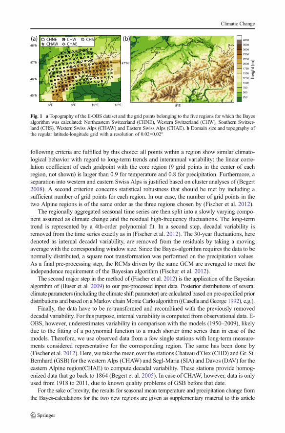
following criteria are fulfilled by this choice: all points within a region show similar climato-logical behavior with regard to long-term trends and interannual variability: the linear corre-lation coefficient of each gridpoint with the core region (9 grid points in the center of eachregion, not shown) is larger than 0.9 for temperature and 0.8 for precipitation. Furthermore, aseparation into western and eastern Swiss Alps is justified based on cluster analyses of (Begert2008). A second criterion concerns statistical robustness that should be met by including asufficient number of grid points for each region. In our case, the number of grid points in thetwo Alpine regions is of the same order as the three regions chosen by (Fischer et al. 2012).
The regionally aggregated seasonal time series are then split into a slowly varying compo-nent assumed as climate change and the residual high-frequency fluctuations. The long-termtrend is represented by a 4th-order polynomial fit. In a second step, decadal variability isremoved from the time series exactly as in (Fischer et al. 2012). The 30-year fluctuations, heredenoted as internal decadal variability, are removed from the residuals by taking a movingaverage with the corresponding window size. Since the Bayes-algorithm requires the data to benormally distributed, a square root transformation was performed on the precipitation values.As a final pre-processing step, the RCMs driven by the same GCM are averaged to meet theindependence requirement of the Bayesian algorithm (Fischer et al. 2012).
The second major step in the method of (Fischer et al. 2012) is the application of the Bayesianalgorithm of (Buser et al. 2009) to our pre-processed input data. Posterior distributions of severalclimate parameters (including the climate shift parameter) are calculated based on pre-specified priordistributions and based on aMarkov chainMonteCarlo algorithm ((Casella andGeorge 1992), e.g.).
Finally, the data have to be re-transformed and recombined with the previously removeddecadal variability. For this purpose, internal variability is computed from observational data. E-OBS, however, underestimates variability in comparison with the models (1950–2009), likelydue to the fitting of a polynomial function to a much shorter time series than in case of themodels. Therefore, we use observed data from a few single stations with long-term measure-ments considered representative for the corresponding region. The same has been done by(Fischer et al. 2012). Here, we take the mean over the stations Chateau d’Oex (CHD) and Gr. St.Bernhard (GSB) for the western Alps (CHAW) and Segl-Maria (SIA) and Davos (DAV) for theeastern Alpine region(CHAE) to compute decadal variability. These stations provide homog-enized data that go back to 1864 (Begert et al. 2005). In case of CHAW, however, data is onlyused from 1918 to 2011, due to known quality problems of GSB before that date.
For the sake of brevity, the results for seasonal mean temperature and precipitation change fromthe Bayes-calculations for the two new regions are given as supplementary material to this article
(b)(a)CHAW CHAE
CHSCHWCHNE
Fig. 1 a Topography of the E-OBS dataset and the grid points belonging to the five regions for which the Bayesalgorithm was calculated: Northeastern Switzerland (CHNE), Western Switzerland (CHW), Southern Switzer-land (CHS), Western Swiss Alps (CHAW) and Eastern Swiss Alps (CHAE). b Domain size and topography ofthe regular latitude-longitude grid with a resolution of 0.02×0.02°
Climatic Change

(Figures 1 and 2 of the Supplementary material). The three probabilistic estimates that areprovided correspond to the 2.5 %-percentile (lower estimate), the median and the 97.5 %-percentile (upper estimate) of the posterior distributions. Figure 9 in the article of (Fischeret al. 2012) shows the same for the regions of Northeastern Switzerland (CHNE), WesternSwitzerland (CHW) and Southern Switzerland (CHS). The Alpine regions CHAW andCHAE show the strongest warming of the five regions in summer under the A1B and A2scenario in the later periods (2045–74 and 2070–99). Model uncertainty, expressed by thespread between the lower and the upper estimate, is similar in all regions. The annual cycleshows a similar pattern with stronger warming in winter and summer as compared to springand autumn. As an example, the projected warming in CHAW for the summer season in2070–99 is 1.3–2.6 °C in RCP3PD, 3.3–5.8 °C in A1B and 3.9–6.7 °C in A2.
A prominent feature in the projections from ENSEMBLES and the derived probabilisticestimates is a height-dependence of temperature change with an increased warming at higheraltitudes (CH2011 2011; Kotlarski et al. 2012b). This is reflected by the regional estimates.The warming tends to be stronger in CHAW and CHAE than in the three non-Alpine regionswith lower average height. For example, the median estimates of temperature change in 2020–49 (2045–74, 2070–99) are about 0.05 °C (0.15 °C, 0.2 °C) larger in winter and about 0.2 °C(0.4 °C, 0.4 °C) larger in summer. Note that these are only regional means. In the ENSEM-BLES multi-model mean, an increased warming of more than 1 °C between the lowest and thehighest points may be found, in particular towards the end of the century.
The precipitation change in the seasonal and regional mean also shows a similar pattern inall five regions. The drier conditions in summer are consistent for the periods 2045–74 and2070–99 in A1B and A2. For example, a possible precipitation reduction by the end of thecentury of about 30 % is found in A2. Note that in general, region CHAW has the smallestuncertainty range in precipitation. This is partly associated with the fact that in CHAWseasonal mean precipitation amounts are the largest and thus, variability in relative terms issmaller than in other regions.
A height-dependence of the precipitation change signal is also found in many seasons andprojection periods. In winter, the ENSEMBLES mean shows a stronger increase in precipita-tion at low altitudes as compared to the Alpine region. For example, an increase of about 10 %in winter is found for the Swiss lowlands, whereas in the Alps the precipitation does notchange at all. Hence, the relative increase in winter precipitation from ENSEMBLES isexpected to be smaller with increasing altitude. The opposite is found in summer, where atendency towards a weaker drying with increasing altitude is found. Here, the lowest gridpoints in western Switzerland exhibit a drying of about 20 % by the end of the century,whereas the drying at high altitudes hardly exceeds 10 % relative to the reference period 1980–2009. These relationships with height can be again partly explained with the absolute amountof precipitation which increases with altitude as a consequence of orographic forcing andenhanced convection. In a recent study by (Fischer et al. 2014) it has also been shown that thedistinct height response in summer is partly related to different precipitation-type responsesoccurring at lower and higher elevated regions. All in all, assuming a spatially homogeneousabsolute change in precipitation in all seasons, these are the vertical dependencies of therelative changes one would expect.
2.2 Downscaling procedure
To make available more localized climate change information, a downscaling procedure hasbeen developed, using the gridded ENSEMBLES mean data and the probabilistic regionalscenarios from CH2011, as described above. Figure 2 shows schematically how the localization
Climatic Change

is achieved. As an example, the case for the median probabilistic estimate of temperaturechange in fall (SON) for the period 2070–99 and scenario A1B is shown.
In a first step, the ENSEMBLES seasonal mean change pattern over Switzerland isadjusted, such that the regional averages correspond to the probabilistic regional estimates ofCH2011. Hence, the adjusted fields are grid point anomalies of the ENSEMBLES meanchange patterns with respect to the regional estimates. For temperature (precipitation), absolute(relative) differences are used. In case of precipitation, the ratios between the scenario and thereference are downscaled and then transformed back to percentage changes. The adjustmentswith the CH2011 estimates are small in general for all median estimates of temperature andprecipitation because the Bayesian median estimates are very similar to the regional means ofthe ENSEMBLES data. In addition, the differences between the regional means of CH2011and ENSEMBLES are much smaller than the grid point anomalies. For example, the mediantemperature change signal in the three CH2011 regions CHNE, CHW, and CHS of the A1B-scenario in winter (DJF) in the period 2070–99 is 3.64 °C, 3.61 °C and 3.83 °C (CH20112011), respectively, while the ENSEMBLES mean temperature change signal suggests awarming range of roughly 1 °C between the lowest and the highest values over Switzerland.Therefore, differences in the regional means between neighboring regions do not lead toproblematic artificial features as shown for the example in the schematic.
The resulting change patterns on the coarse grid are downscaled using a Kriging interpo-lation with external drift (Journel and Huijbregts 1978; Wackernagel 2003). Kriging is themost prominent technique in geostatistics when dealing with relatively small samples (VonStorch and Zwiers 2002). It is the best linear unbiased predictor for spatially correlated data.Kriging with external drift, often also referred to as Universal Kriging, assumes that thedownscaled pattern is given by the sum of a deterministic part (regression or trend) and astochastic part (kriged trend residuals). Kriging with external drift is similar to OrdinaryKriging, except that the covariance matrix is extended with the values of the auxiliary
Stochastic partDeterministic partLocalized change signal = +
External drift or trend (longitude, latitude, height)
Kriging of residuals(exponential variogram)
ENSEMBLES multi-modelseasonal mean change pattern
regionally adjusted ENSEMBLES seasonal mean change pattern
with CH2011 estimates
Fig. 2 Schematic of downscaling procedure. The method is illustrated for the median probabilistic estimate oftemperature change in fall (SON) for the period 2070–99 and scenario A1B
Climatic Change

predictors. The regression is based on generalized least squares because of spatial correlationin the data.
For an estimation of the deterministic part of the climate change signals, the geographicalcoordinates longitude, latitude and height on the coarse ENSEMBLES grid are used aspredictors. The height of the E-OBS data instead of the ENSEMBLES mean is used here.This is because the orography in the multi-model mean slightly differs prior to and after 2050due to the unequal number of RCM-GCM-chains. In the ENSEMBLES/E-OBS data thehighest values do not exceed 2,600 m asl, whereas the highest Alpine elevations in the 2-km grid are above 4,000 m asl. The regression is used to extrapolate in this range.
In order to test whether or not height should be included as a linear predictor, likelihoodratio tests were performed for each estimate. The likelihood ratio test compares the likelihoodL of two statistical models of different complexity, one of which is nested into the other(Neyman and Pearson 1933). The corresponding test statistic D is twice the ratio of the log-likelihoods of the two models:
D ¼ −2lnL0 Θð ÞL1 Θð Þ
� �ð1Þ
The probability distribution ofD can be approximated with a χ2 -distribution with (df0−df1)degrees of freedom, where df0 and df1 are the degrees of freedom of the null model withlikelihood function L0(Θ) and the model of higher complexity denoted by L1(Θ). Here, thedownscaling procedure was once performed with height included and once without. For bothtemperature and precipitation more than 80 % of p-values is below the 5 %-significance level,meaning that the null model (without height) is most often rejected. Therefore, height isneeded as an additional predictor to explain the spatial variability of temperature and precip-itation change in the (adjusted) ENSEMBLES mean patterns over Switzerland. Note that anyhigher-order polynomial terms of height do not generally improve the downscaling further andmight lead to overfitting.
The kriged residuals can be interpreted as spatially correlated local deviations from thedeterministic trend. They build the stochastic component. The spatial correlation is modeledwith omnidirectional empirical variograms that are computed individually for each estimate.The fitted exponential variograms are based on maximum likelihood estimation.
For the construction of the localized climate change signals under the greenhouse gasemission scenarios A2 and RCP3PD, the ENSEMBLES mean change patterns have beenscaled from A1B with the same pattern-scaling factors as used by (Fischer et al. 2012). Thefactors for A2 (RCP3PD) are 0.89 (0.95) for the period 2020–49, 0.98 (0.60) for 2045–74 and1.17 (0.43) for 2070–99.
In order to avoid boundary effects to occur within Switzerland in the Kriging step, variousgrid points outside the country borders are taken into account (see Fig. 1a). Finally, the areasoutside of Switzerland in the localized data are removed for further analysis.
2.3 Proof of concept
Uncertainties associated with the downscaling procedure are discussed below. Here, theusefulness of the downscaling method with respect to the Kriging step is confirmed with thetest illustrated in Fig. 3. The difference between the observed seasonal mean temperature of thetwo norm periods 1981–2010 and 1961–1990 is considered as a ‘perfect model simulation’ ofpast temperature change (Fig. 3a–d). More details on the establishment of the new norm period1981–2010 is provided by (Begert et al. 2013). The original data for the two periods is given
Climatic Change

on the high-resolution grid. For this test, the observed change signals were first upscaled bygrid cell averageing to the 0.22° grid of the ENSEMBLES models (Fig. 3e–h) and thendownscaled with the Kriging method described above (Fig. 3i–l).
If the downscaling procedure were perfect and all climatological information wereavailable on the coarser grid, the panels in Fig. 3(i–l) would be equal to the respectivepanels in the top row and the bias would be zero. It is shown that the patterns are roughlyreconstructed by the downscaling in all seasons. The kriging step contributes to a consid-erable degree of smoothing in the lower Rhone valley, where very small-scale features canbe discerned in the original data. However, the slightly stronger warming in the Swisslowlands as compared to the surrounding higher regions is well captured. In addition, thedownscaling scheme is able to reproduce the warming pattern in the western Ticino insummer. The bias is largely below ±0.2 °C.
(a) DJF
(e) DJF
(i) DJF
(b) MAM
(f) MAM
(j) MAM
(c) JJA
(g) JJA
(k) JJA
(d) SON
(h) SON
(l) SON
ORIGINAL
UPSCALED
DOWNSCALED
Temperature (°C)
Temperature bias (°C)
(DOWNSCALED - ORIGINAL)(m) DJF (n) MAM (o) JJA (p) SON
Fig. 3 Seasonal mean temperature change between the period 1981–2010 and 1961–1990 for winter (DJF),spring (MAM), summer (JJA) and fall (SON). Top row (a–d): original data on 0.02° grid, second row (e–h):original values upscaled to 0.22° ENSEMBLES grid by grid box averageing, third row (i–l): downscaled valueson high-resolution grid, bottom row (m–p): bias of downscaling method (downscaled signal minus original data)
Climatic Change

Good agreement between original and downscaled temperature change pattern is also foundin fall (SON). Very small-scale differences, e.g. in the Rhine valley and the surroundingmountains, are quite well reproduced. In the observations, fall is the only season showing astatistically significant height-dependence of the temperature change between the two refer-ence periods. This is in contrast to the projected future change signals from ENSEMBLES,where the height-dependence is significant inmost seasons for both temperature and precipi-tation as shown above with the likelihood ratio tests. Hence, since a significant height-dependence seems important for a successful downscaling of valley/ridge features, we areconfident that for the projected change signals this approach produces reasonable results.
A corresponding proof of concept for precipitation is provided as Supplementary material(Fig. 3). Also for the case of precipitation the changes on the regional scale are well capturedby the kriging method. On local scale, the original change pattern in the observations is verypatchy as a consequence of changes in station density over time and aspects of interpolationfrom stations to the 2-km grid. This results in small likelihood values in the kriging methodand relatively large local biases of up to 8 %.
2.4 Uncertainties of the downscaling method
There are several sources of uncertainty in the localized climate change signals. The majorsource of uncertainty can be traced back to the posterior distribution of the climate changesignals obtained from the Bayesian algorithm. The distribution is very sensitive to the priorchoice of the model projection uncertainty as shown by (Fischer et al. 2012). The spreadbetween the lower and the upper probabilistic estimate depends on the prior variance assumed.(Fischer et al. 2012) illustrate that depending on the chosen model projection uncertainty andthe number of models, a difference in the confidence intervals of 1–5 °C is possible fortemperature. For precipitation, model projection uncertainty also largely contributes to theoverall uncertainty. An additional contribution is given by the recombination with internaldecadal variability from station observation, as discussed above. As a consequence, the threeestimates should not be interpreted in a strictly probabilistic way. They should be considered asthree equally likely realizations of temperature or precipitation change in Switzerland (CH20112011).
Much smaller uncertainties are induced by the downscaling method on the localized scale.These uncertainties are associated with the stochastic component of the Universal Kriginginterpolation onto the 2-km grid. Based on the fitted exponential variograms, the weightingcoefficients for the interpolation are computed. They are subject to uncertainty. The Krigingstandard deviation can be used as a measure to quantify uncertainties due to the downscalingapproach for each individual realization discussed beforehand.
Figure 4a–b depict the change signals for the median estimates of temperature andprecipitation by the end of the century (2070–99) for the A1B-scenario. The change signalsare displayed as average values within height bins of 500 m thickness. Attached to each meanvalue is an uncertainty bar. It corresponds to the mean value of the bin±1 Kriging standarddeviation. Since the Kriging standard deviation is different for each grid point and by designapproaches zero near the grid points of the coarse ENSEMBLES grid, the method stronglyconstrains the downscaled climate change signals to the patterns found on the coarse grid. Thisincludes regions above 2,600 m asl, where an extrapolation is done. Hence, the maximum ofthe standard deviations in each height bin is used in the plot. First of all, this plot shows thestrong vertical dependence of the climate change signals in all seasons under the A1B-scenarioat the end of the century. Secondly, the uncertainty range defined through the maximalstandard deviation in temperature (precipitation) does not exceed 0.3 K (4 %) in these cases.
Climatic Change

Uncertainties tend to be very slightly larger at higher altitudes (mostly less than +0.03 K fortemperature and +0.1 % for precipitation). For temperature, the uncertainty of the Kriging stepis comparable in magnitude to the bias obtained for the proof of concept with observed thetemperature changes. It is also noteworthy that the vertical dependence of the climate changesignals is substantially larger in all displayed cases than the respective uncertainty ranges.
Figure 4c–d show histograms over all estimates (all seasons, periods and scenarios) for themaximum Kriging standard deviation over Switzerland for temperature and precipitation. It isobvious that in general the uncertainty associated with the Kriging method is very small. Morethan 80 % of all estimates have standard deviations of less than 0.15 K in case of temperatureand less than 2 % in case of precipitation. These standard deviations are roughly by a factor 2to 10 smaller than the vertical dependence when the latter is expressed in terms of maximumdistance between largest and smallest change signal for a given estimate.
−25
−20
−15
−10
−50
510
Prec
ipita
tion
chan
ge [%
]
<500
500−
1000
1000
−150
0
1500
−200
0
2000
−250
0
2500
−300
0
3000
−350
0
>350
0
(b) Change signal for precipitation (A1B, 2070−99, median)
Height levels [m]
2.0
2.5
3.0
3.5
4.0
4.5
5.0
Tem
pera
ture
cha
nge
[K]
<500
500−
1000
1000
−150
0
1500
−200
0
2000
−250
0
2500
−300
0
3000
−350
0
>350
0
(a) Change signal for temperature (A1B, 2070−99, median)
Height levels [m]
DJFMAM
JJASON
(c) Histogram of Kriging standard deviation (temperature)
Temperature [K]
Den
sity
0.00 0.05 0.10 0.15 0.20 0.25 0.30
0.0
0.1
0.2
0.3
0.4
(d) Histogram of Kriging standard deviation (precipitation)
Precipitation [%]
Den
sity
0.5 1.0 1.5 2.0 2.5 3.0 3.5 4.0
0.00
0.05
0.10
0.15
0.20
0.25
0.30
0.35
Fig. 4 Change signals for the median estimates of a temperature and b precipitation by the end of the century(period 2070–99) for the A1B-scenario and histograms of Kriging standard deviation for all estimates of ctemperature and d precipitation. In (a) and (b) the dots correspond to mean values over height bins of 500 mthickness. The respective lines indicate Kriging uncertainty: the maximal standard deviation of each height bin isadded or subtracted from the mean value. The total density in (c) and (d) amounts to 1
Climatic Change

Additional uncertainties are connected to the fact that (1) the ENSEMBLES mean pattern isused rather than single model output and that (2) a simple pattern-scaling approach is used forthe scenarios A2 and RCP3PD. In order to quantify the uncertainties associated with the use ofmulti-model mean data (point 1), the downscaled mean pattern was compared against themean over all models downscaled with the same method. The root mean squared error(RMSE) for the median estimate of scenario A1B (period 2070–99) was found to be0.04 °C (0.05 °C, 0.11 °C, 0.08 °C) for temperature in DJF (MAM, JJA, SON) and 4.1 %(3.0 %, 1.4 %, 4.1 %) in DJF (MAM, JJA, SON) for precipitation. Uncertainties in earlierprojection periods are of the same order or smaller. Concerning point (2), (Fischer et al. 2012)found uncertainties of the pattern-scaling procedure in the order of 0.2 K for temperature and6 % for precipitation.
3 Results
The resulting localized climate change signals for seasonal averages of daily mean temperatureare shown in Fig. 5. For the sake of brevity, only the A1B scenario is displayed here. Thewarming clearly increases towards the end of the 21st century, from about 1 °C in 2020–2049with respect to the reference period 1980–2009 to roughly 4 °C in 2070–2099 (medianestimate). The annual cycle of the change signal for temperature is not pronounced, althougha slightly stronger warming is found for the summer season. This finding is independent of thechosen scenario or scenario period. In A1B and A2, the associated model uncertainty of the
2020-2049
2045-2074
2070-2099
reppunaidemrewol
DJF
JJA
MAM
SON
DJF
JJA
MAM
SON
DJF
JJA
MAM
SON
DJF
JJA
MAM
SON
DJF
JJA
MAM
SON
DJF
JJA
MAM
SON
DJF
JJA
MAM
SON
DJF
JJA
MAM
SON
DJF
JJA
MAM
SON
Fig. 5 Localized seasonal mean temperature change signals for the A1B scenario. The lower, median and upperestimate (initially derived from 2.5 %-, 50 %- and 97.5 %-quantile) for each of the three scenario periods (2020–2049, 2045–2074, and2070-2099)
Climatic Change

change signal, expressed here by the lower and upper estimate, increases towards the end ofthe century. In the RCP3PD scenario the change signals hardly differ between the differentperiods. Note, that by design these results agree with the CH2011 report (CH2011 2011).
The height-dependence of the change signal in the ENSEMBLES models can partly beassociated to the snow-albedo feedback and other mechanisms (Ceppi et al. 2012; Kotlarskiet al. 2012a). The snow-albedo feedback describes the enhanced warming with less snow dueto a darker land surface and the connected increase in absorbed solar radiation at the surface(Im et al. 2011). Thus, the warming is larger at higher altitudes, where the models predict asnow cover decrease in the future (Im et al. 2011; Ceppi et al. 2012; Kotlarski et al. 2012a;Steger et al. 2013). In summer, the warming in 2045–2074 and also 2070–2099 is about 1 °Clarger above 2,500 m asl as compared to the Swiss lowlands with altitudes between 400 and800 m asl. This is also confirmed by Fig. 4. The largest difference in space results between thesouthwestern mountains along the border to Italy and the northeastern lowlands close to LakeConstance. Despite the physical explanation for the enhanced warming at higher altitude in theENSEMBLES models, one has to be aware that the signal above 2,600 m asl is a result of thestatistical extrapolation.
Given the vertical gradient in warming, the most remarkable difference between thespatially localized dataset and the ENSEMBLES mean pattern can be expected in the Alpineregion, with its complex topography including mountains higher than 4,000 m asl but alsodeep and narrow valleys with altitudes down to 400 m asl. One such example is the Rhoneriver valley that is flanked to both sides by the highest mountains of the Valaisan and theBernese Alps. This valley is not resolved by the ENSEMBLES models owing to the fact thatthe valley ground is rather narrow with less than 6 km width. As an example, in the A1B-scenario in summer during 2070–99 the Rhone river valley warms about 1 °C less than itshighest surrounding peaks (median estimate).
For each probabilistic estimate, the observed and projected temperature values for winterand summer assuming the A1B scenario (2070–99) are given as Supplementary material(Fig. 4). In this approach, the values in the scenario period are simplythe observations shiftedby the collocated change signal. The increase in temperature by the end of the century causes aretreat of the zero-degree line towards the core of the Alpine region. It also rises about 400 min the median estimate of A1B (2070–99), such that the vast majority of hills north of the Alpsmay be above 0 °C mean temperature during winter. In summer, daily average temperaturesabove 20C are projected to be normal in the Swiss lowlands, the Rhone river valley, as well asthe Ticino.
Figure 6 shows the downscaled climate change signals of mean precipitation for the A1Bemission scenario (2070–99) on the 2-km grid. Precipitation change can be both positiveor negative. Natural decadal variability that amounts to roughly±10 % is hardly exceededin most seasons (CH2011 2011). During the summer season a distinct drying is projected.The summer drying is enhanced towards the end of the century. It is strongest in thewestern part of Switzerland and south of the Alps. Previous studies suggested that thesummer drying in most of southern and central Europe is a consequence of the expansionand weakening of the Hadley cell (Held and Soden 2006; Lu et al. 2007; Mariotti et al.2008; CH2011 2011) and the associated increase in moisture divergence across thesubtropical dry zone in response to the greenhouse gas forcing and the associated stabi-lization of the tropical and subtropical atmosphere (Lu et al. 2007). This is seen in allGCMs of the IPCC fourth Assessment Report (Solomon et al. 2007). In addition, apositive soil-moisture-precipitation feedback is projected to enhance the reduction ofconvective summer precipitation, and thus, support the northward expansion of theaforementioned dry zone (Rowell and Jones 2006).
Climatic Change

In winter, a slight precipitation increase in the median estimate in the Swiss lowlands (5–10 %) and south of the Alps (up to 20 %) is projected by the end of the century. Possibleexplanations for the wetter conditions in future winter seasons are the increase in atmosphericmoisture content due to the higher water holding capability of the warmer atmosphere andcirculation changes.
The observed mean winter and summer precipitation as well as the projected futureprecipitation using the A1B scenario are shown in the Supplementary material to this article(Fig. 5).
4 Discussion
A new spatially localized data set of climate change signals for seasonal mean temperature andprecipitation in Switzerland was presented. A Kriging interpolation with external drift wasused to downscale the ENSEMBLES mean climate change patterns with a resolution ofroughly 25 km in combination with a Bayesian method for larger regions to a grid withhorizontal resolution of about 2 km. Height is used as an auxiliary predictor to take intoaccount the elevation dependence of the climate change signal. This is strongly motivated bythe complex topography not represented by the given regional climate models.
The new data set allows to distinguish differences in the mean climate change signalbetween Alpine valleys and mountain ridges and, thus, facilitates the study of more complexlocal and regional climate change within Switzerland, e.g. the impact ofthe warming atmo-sphere on glacier development, river discharge, agricultural and other aspects at a finehorizontal scale.
2020-2049
2045-2074
2070-2099
reppunaidemrewol
DJF
JJA
MAM
SON
DJF
JJA
MAM
SON
DJF
JJA
MAM
SON
DJF
JJA
MAM
SON
DJF
JJA
MAM
SON
DJF
JJA
MAM
SON
DJF
JJA
MAM
SON
DJF
JJA
MAM
SON
DJF
JJA
MAM
SON
%
Fig. 6 The same as Fig. 5, but for precipitation (%)
Climatic Change

We found a distinct altitude-dependence of both temperature and precipitation changesignals. The magnitude of the dependence on altitude, however, is different for the fourseasons and the three scenario periods. A maximum difference between the lowlands andthe highest mountain peaks of about 1 °C was found for summer in 2045–2074 and 2070–2099, likely caused by local feedback processes such as the snow-albedo feedback ((Kotlarskiet al. 2012a), e.g.).
We highlighted the benefit of having such a data set for the Alpine region, wherethe amplitude of the climate change signals can vary between the valleys and thesurrounding mountain peaks. However, the present study clearly has limitations. Firstof all, it relies on seasonal mean quantities. The interannual variability and changesthereof are not considered. Also, the results do not allow statements about changes intemporal correlations on a daily time scale. However, the seasonal mean change signalcan directly be applied to daily time series using a delta-change approach. Thelimitations of such a procedure must be considered though: Altering standard devia-tions or temporal and spatial correlations are not taken into account, neither arechanges in dry or wet spell lengths considered. Furthermore, the presented approachassumes a constant bias, an assumption which may be problematic for some regionalclimate models run within the ENSEMBLES project (Christensen et al. 2008).
Another limitation is given by the use of height alone as a linear predictor because it is notthe only factor affecting climate change in the Alps. There is a relatively large range ofaltitudes between 2,600 and 4,000 m asl, where extrapolation is necessary because theENSEMBLES mean orography does not go beyond 2,600 m asl. On the one hand, anextrapolation is desired, as studies of warming on high spatial resolution in the Alps haveshown an altitude-dependence of the climate change signal ((Im et al. 2011), e.g.), who used aregional climate model at 3-km resolution. On the other hand, extrapolation is used for dataimputation at locations, where no data is available in the input data set, and thus, local-scalechanges in individual grid cells must be treated carefully. Also, the choice of the downscalingmethod and the parameter estimation add uncertainty that has to be quantified. In this study,the largest source of uncertainty for the climate change signals is induced by the ensemble ofRCMs and is largely determined by the prior assumptions made within the Bayes algorithm(model projection uncertainty).
Uncertainties associated with the Kriging method and the choice of the ENSEM-BLES mean patterns rather than single model output were found to be comparativelysmall. Kriging standard deviations are of the order of 0.1 K for temperature or 2–4 %and less for precipitation. Thus, we have confidence that the method chosen forlocalization of the height-dependent climate change signals produces reasonable androbust results.
When using the data set, one should keep in mind that the three seasonal estimates providedfor each scenario and projection period should be interpreted as equally likely realizations ofclimate change rather than events with a certain probability. In addition, potential users shouldbe aware that temperature and precipitation were downscaled independently of each other inthis study. Further studies should treat temperature and precipitation in a bivariate approach tomake sure that correlations between the two quantities are taken into account. Nevertheless,despite the abovementioned uncertainties and limitations the new data set enables a variety ofinteresting studies of local climate change in Switzerland. An application of the data set for anumber of relevant climate change indices is provided by (Zubler et al. 2014).
Acknowledgments The author wishes to thank the anonymous reviewers for their valuable comments. TheCH2011 data were obtained from the Center for Climate Systems Modeling (C2SM). The ENSEMBLES data
Climatic Change

used in this work was funded by the EU FP6 Integrated Project ENSEMBLES(Contract number 505539) whosesupport is gratefully acknowledged. The Swiss Federal Office for the Environment (FOEN) is partly financingthe present study.
Open Access This article is distributed under the terms of the Creative Commons Attribution License whichpermits any use, distribution, and reproduction in any medium, provided the original author(s) and the source arecredited.
References
Baeriswyl PA, Rebetez M (1997) Regionalization of precipitation in Switzerland by means of principalcomponent analysis. Theor Appl Climatol 58:31–41
Begert M (2008) Repräsentativität der Stationen im Swiss National Basic Climatological Network.Arbeitsberichte der MeteoSchweiz 217, MeteoSwiss
Begert M, Schlegel T, Kirchhofer W (2005) Homogeneous temperature and precipitation series of Switzerlandfrom 1864 to 2000. Int J Climatol 25:65–80
Begert M, Frei C, Abbt M (2013) Einführung der Normperiode 1981–2010. Fachbericht 245, MeteoSchweizBeniston M, Rebetez M (1996) Regional behavior of minimum temperatures in Switzerland for the period 1979–
1993. Theor Appl Climatol 53:231–244Buser CM, Künsch HR, Lüthi D, Wild M, Schär C (2009) Bayesian multi-model projections of climate: bias
assumptions and interannual variability. Clim Dyn 33:849–868. doi:10.1007/s00382-009-0588-6Casella G, George E (1992) Explaining the Gibbs sampler. Am Stat 46(3):167–174Ceppi P, Scherrer SC, Fischer A, Appenzeller C (2012) Revisiting Swiss temperature trends 1959–2008. Int J
Climatol 32:203–213. doi:10.1002/joc.2260CH2011 (ed) (2011) Swiss Climate Change Scenarios CH2011. C2SM, MeteoSwiss, ETH, NCCR Climate, and
OcCC, Zurich, SwitzerlandChristensen JH, Boberg F, Christensen OB, Lucas-Picher P (2008) On the need for bias correction of regional
climate change projections of temperature and precipitation. Geophys Res Lett 35(L20709), doi:10.1029/2008GL035694
Fischer EM, Schär C (2010) Consistent geographical patterns of changes in high-impact European heatwaves.Nat Geosci 3:398–403. doi:10.1038/ngeo866
Fischer AM, Weigel AP, Buser CM, Knutti R, Künsch HR, Liniger MA, Schär C, Appenzeller C (2012) Climatechange projections for Switzerland based on a bayesian multi-model approach. Int J Climatol 32(15):2348–2371. doi:10.1002/joc.3396
Fischer AM, Keller DE, Liniger MA, Rajczak J, Schär C, Appenzeller C (2014) Projected changes inprecipitation intensity and frequency in Switzerland: a multi-model perspective. submitted to Int J Climatol
FOEN (2012) Adaptation to climate change in Switzerland - goals, challenges and fields of action: First part ofthe Federal Council’s strategy. Tech. rep., Federal Office for the Environment
Frei C (2013) Interpolation of temperature in a mountainous region using non-linear profiles and non-euclideandistances. Int J Climatol. doi:10.1002/joc.3786
Giorgi F, Hurrell JW, Marinucci MR (1997) Elevation dependency of the surface climate change signal: a modelstudy. J Clim 10:288–296
Haylock MR, Hofstra N, Tank AMGK, Klok EJ, Jones PD, New M (2008) A European daily high-resolutiongridded data set of surface temperature and precipitation for 1950–2006. J Geophys Res 113(D20119), DOI10.1029/2008jd010201
Held IM, Soden BJ (2006) Robust responses of the hydrological cycle to global warming. J Climate 19:5686–5699, http://dx.doi.org/10.1175/JCLI3990.1
Im ES, Coppola E, Giorgi F, Bi X (2011) Local effects of climate change over the alpine region: A study with ahigh resolution regional climate model with a surrogate climate change scenario. Geophys Res Lett 37(5),doi:10.1029/2009GL041801
Jasper K, Calanca P, Gyalistras D, Fuhrer J (2004) Differential impacts of climate change on the hydrology oftwo alpine river basins. Clim Res 26:113–129
Journel AG, Huijbregts C (1978) Mining geostatistics. Academic, New YorkKöplin N, Viviroli D, Schädler B, Weingartner R (2010) How does climate change affect mesoscale catchments
in Switzerland? - a framework for a comprehensive assessment. Adv Geosci 27:111–119. doi:10.5194/adgeo-27-111-2010
Climatic Change

Kotlarski S, Bosshard T, Lüthi D, Pall P, Schär C (2012a) Elevation gradients of European climate change in theregional climate model COSMO-CLM. Clim Chang 112:189–215. doi:10.1007/s10584-011-0195-5
Kotlarski S, Lüthi D, Schär C (2012b) The dependence of 21st century European climate change on surfaceelevation - an RCM ensemble analysis. In: EGU General Assembly, European Geophysical Union (EGU),Vienna, Austria, p 4356
Lu J, Vecchi G, Reichler T (2007) Expansion of the Hadley cell under global warming. Geophys Res Lett 34(6):L06,805
Mariotti A, Zeng N, Yoon JH, Artale V, Navarra A, Alpert P, Li LZX (2008) Mediterranean water cycle changes:transition to drier 21st century conditions in observations and CMIP3 simulations. Environ Res Lett3(044001)
Meehl GA, Stocker TF, Collins WD, Friedlingstein P, Gaye AT, Gregory JM, Kitoh A, Knutti R, Murphy JM,Noda A, et al. (2007) Climate Change 2007: The Physical Science Basis. Contribution of Working Group Ito the Fourth Assessment Report of the Intergovernmental Panel on Climate Change, Cambridge UniversityPress, 32 Avenue of the Americas, New York, NY 10013–2473, USA, chap Chapter 10: Global climateprojections, pp 747–845
Meinshausen M, Smith SJ, Calvin KV, Daniel JS, Kainuma MLT, Lamarque JF, Matsumoto K, Montzka SA,Raper SCB, Riahi K, Thomson AM, Velders GJM, van Vuuren D (2011) The RCP greenhouse gasconcentrations and their extension from 1765 to 2300. Clim Chang. doi:10.1007/s10584-011-0156-z,Special Issue
Neyman J, Pearson ES (1933) On the problem of the most efficient tests of statistical hypotheses. Philos Trans RSoc A: Math Phys Eng Sci 231:289–337. doi:10.1098/rsta.1933.0009.JSTOR91247
Rangwala I, Miller JR (2012) Climate change in mountains: a review of elevation-dependent warming and itspossible causes. Clim chang 114(3–4):527–547
Rebetez M, Reinhard M (2011) Monthly air temperature trends in Switzerland 1901–2000 and 1975–2004.Theor Appl Climatol 91:27–34. doi:10.1007/s00704-007-0296-2
Rowell DP, Jones RG (2006) Causes and uncertainty of future summer drying over Europe. Clim Dyn 27(2–3):281–299
Schär C, Vidale PL, Lüthi D, Frei C, Häberli C, Liniger MA, Appenzeller C (2004) The role of increasingtemperature variability in European summer heatwaves. Nature 427(6972):332–336
Scherrer S, Ceppi P, Croci-Maspoli M, Appenzeller C (2012) Snow-albedo feedback and Swiss spring temper-ature trends. Theor Appl Climatol 110(4):509–516
Schmidli J, Frei C (2005) Trends of heavy precipitation and wet and dry spells in Switzerland during the 20thcentury. Int J Climatol 25:753–771. doi:10.1002/joc.1179
Schüepp M, Gensler G (1980) Klimaregionen der Schweiz. In: Müller G (ed) Die Beobachtungsnetze derSchweizerischen Meteorologischen Anstalt, no. 93 in Arbeitsbericht der Schweizerischen MeteorologischenZentralanstalt, Schweizerische Meteorologische Anstalt, Zürich
Solomon S, Qin D, Manning M, Chen Z, Marquis M, Averyt K, Tignor M, Miller H (eds) (2007) ClimateChange 2007: The Physical Science Basis. Contribution of Working Group I to the Fourth AssessmentReport of the Intergovernmental Panel on Climate Change. Cambridge University Press, 32 Avenue of theAmericas, New York, NY 10013–2473, USA
Steger C, Kotlarski S, Jonas T, Schär C (2013) Alpine snow cover in a changing climate: a regional climatemodel perspective. Clim Dyn 41:735–754
van der Linden P, Mitchell JFB (2009) ENSEMBLES: climate change and its impacts: summary of research andresults from the ENSEMBLES project. Met Office Hadley Centre, Exeter. doi:10.1029/2004GL020255
Von Storch H, Zwiers FW (2002) Statistical analysis in climate research. Cambridge University PressWackernagel H (2003) Multivariate geostatistics. SpringerZubler EM, Scherrer SC, Croci-Maspoli M, Liniger MA, Appenzeller C (2014) Key climate indices in
Switzerland; expected changes in a future climate. Clim Change pp 1–17, doi:10.1007/s10584-013-1041-8, URL http://dx.doi.org/10.1007/s10584-013-1041-8
Climatic Change