literature mass lapse scenario in insurance, the use of a ... · xavier milhaud introduction key...

Surrenders

Xavier Milhaud

IntroductionKey ideasLiteratureMain threatsA-prioriIssues

ExistingapproachesTablesQIS5Extensions

Correlation crisisConceptCommon shocksHawkes processes

Conclusion

References

References

Mass lapse scenario in insurance, the use of adynamic contagion process

Séminaire de la Chaire ACPRParis, le 6 janvier 2015

Xavier Milhaud1,2

Joint work with F. Barsotti and Y. Salhi

1 CREST - Laboratoire de Finance et d’Assurance2 ENSAE ParisTech

1/37

Surrenders

Xavier Milhaud




Conclusion

References

References

Outline

1 Introduction to the problem

2 Current approaches in companies

3 Correlation crisis

4 Key messages, limits and on-going research

2/37

Surrenders

Xavier Milhaud




Conclusion

References

References

A word on the surrender risk

FIRSTLY: what is the SURRENDER RISK?

Why is the insurer interested in understanding this risk?

1 For the design of new products,to set up assumptions on the average surrender rate,because it has a straight impact on A.L.M. and E.E.V.

2 To understand the behaviours,main discriminating factors of surrenders? CARTbehaviour risk essential (adapt product features to gainmarket shares).

3 Predictions: risk segmentation and management.better assess the surrender risk at underwriting process,be able to quantify the surrender probability wheneverwe would like during the contract lifetime.

Our aim is to extract triggers, classify and predict surrenders.

3/37

Surrenders

Xavier Milhaud




Conclusion

References

References

Some key-points

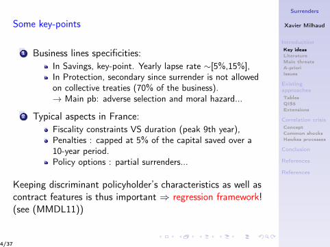
1 Business lines specificities:In Savings, key-point. Yearly lapse rate ∼[5%,15%],In Protection, secondary since surrender is not allowedon collective treaties (70% of the business).→ Main pb: adverse selection and moral hazard...

2 Typical aspects in France:Fiscality constraints VS duration (peak 9th year),Penalties : capped at 5% of the capital saved over a10-year period.Policy options : partial surrenders...

Keeping discriminant policyholder’s characteristics as well ascontract features is thus important ⇒ regression framework!(see (MMDL11))

4/37

Surrenders

Xavier Milhaud




Conclusion

References

References

Existing literature in modelling surrenders

The 2 main historical explanations for surrenders are liquidityneeds (Out90) and rise of interest rates (obvious...)

There are 4 different approaches to model surrenders:Finance (TKC02), (Kue05), (BBP08) : price surrenderoption, optimal and rational behaviours assumption,Statistics (RH86), (FLP07): collective. Empirical dataallow to calibrate surrender functions like:

rd = r0 ∗ (1− a ∗ ln(d) ∗ (ln(d + 1)− b))

Economics (FLP07): microeconomy, expected utilitytheory, rational behaviour. But is it really like this?Econometrics (CL06), (Kim05), (Kag05): individual.

segmentation models to define risk classes,GLM to quantify the impact of risk factors,intensity models (see also prepayment for mortgages).

5/37

Surrenders

Xavier Milhaud




Conclusion

References

References

Threats for Life insurers (rachats conjoncturels)

Remaining questions:how did the financial crisis impact the surrender rates?do financial markets strongly impact policyholders’behavior? Very difficult to answer...

Current context:never experienced such low interest rates,⇒ underwriting of new business has been done withthese abnormal low rates since 4 years,Surrenders could be forbidden by the regulatory⇒ could lead policyholders to invest differently, andmakes life insurance investments become less attractive.

Major issue: face massive surrenders due to a suddenincrease of rates (how to adapt contracts, market shares...).

6/37

Surrenders

Xavier Milhaud




Conclusion

References

References

Intuitions

The surrender behaviours are mainly driven by two riskclasses: fiscality constraints and financial markets → sourcesfrom two different areas:

endogenous or idiosynchratic factors: surrender feesprofile, tax relief, contract options, distribution channel,customer segment, cross-selling → structural surrenders;exogenous or environmental factors: financial markets,reputation risk and bankruptcy fear, regulatory changes→ temporary surrenders.

From our experience,

=⇒ GLM fail into modelling such a complex dependence,especially because of exogenous factors (see next slide).

=⇒ Survival models do not catch the heterogeneity of thedata, even if we use frailty models.

7/37

Surrenders

Xavier Milhaud




Conclusion

References

References

Ex.: dynamic logit on Spanish endowments

Model statistically significant, predictions dramatically bad!

2000 2001 2002 2003 2004 20052000 2001 2002 2003 2004 20052000 2001 2002 2003 2004 20052000 2001 2002 2003 2004 2005

date

surr

ende

r ra

te

0%2%

4%6%

8%

Observed surr. rateModeled surr. rate95 % confidence interval

Learning sample (month basis),Mixtos products (All)

2006 20072006 20072006 20072006 2007

date

surr

ende

r ra

te

0%2%

4%6%

8%

Observed surr. rateModeled surr. rate95 % confidence interval

Validation sample (month basis),Mixtos products (All)

→ Correct model as long as everything remain stable, but...→ Financial crisis not captured by the model (althoughfinancial variables input as covariates). Correlation (??).

8/37

Surrenders

Xavier Milhaud




Conclusion

References

References


2 Current approaches in companiesStatistics on segments for structural surrendersApproche QIS 5Ideas from “Orientations nationales complémentaires duQIS 5”



9/37

Surrenders

Xavier Milhaud




Conclusion

References

References

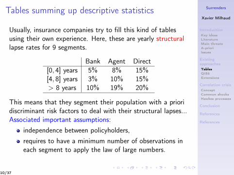
Tables summing up descriptive statistics

Usually, insurance companies try to fill this kind of tablesusing their own experience. Here, these are yearly structurallapse rates for 9 segments.

Bank Agent Direct[0, 4] years 5% 8% 15%[4, 8] years 3% 10% 15%> 8 years 10% 19% 20%

This means that they segment their population with a prioridiscriminant risk factors to deal with their structural lapses...Associated important assumptions:

independence between policyholders,requires to have a minimum number of observations ineach segment to apply the law of large numbers.

10/37

Surrenders

Xavier Milhaud




Conclusion

References

References

CEIOPS (EIOPA) - QIS 5 - Calibration papers

Recommendations for capital requirements are computed inTWO steps (cf p.105).

(1) Shocks up / down applied to structural lapse rate:

Following empirical studies in 2003 in UK on individualwith-profit life insurance policies (and also in Poland), thestructural lapse rate should be shocked in the following way:

LRup = min(100%, 150%× LR),

LRdown = min(0,max(50%× LR, LR − 20%)).

→ Should cover misestimation or permanent changes of LR.→ Incorporates temporary lapses!

11/37

Surrenders

Xavier Milhaud




Conclusion

References

References

CEIOPS (EIOPA) - QIS 5 - Calibration papers

(2) Mass lapse event:

Corresponds to the deterioration of a financial position of theundertaking, reputation ∼ “bank run” (Northern Rock!),“catastrophe type event”...

→ Empirical basis to calibrate mass lapse event is very poor(or never observed...);→ It is advised to consider a loss of 30% of the sum ofpositive surrender strain over the portfolio;→ It should be adjusted to the type of life insurance policy,e.g with-profit contract usually have higher persistency...

→ Also incorporates temporary lapses!

We keep as required capital the maximum capital to reservecorresponding to all these scenarii ((1) and (2)).

12/37

Surrenders

Xavier Milhaud




Conclusion

References

References

Other suggestion for managing lapse rates:Orientations nationales complémentaires du QIS 5

Temporary lapses in addition to structural lapses by:

Modèle ALM : Apport de la Logique Floue dans la modélisation des comportements

y remédier, l’ACP a proposé dans les orientations nationales complémentaires du QIS 5, une loide rachat conjoncturel en fonction du spread de taux qui peut exister entre le taux servis parl’assureur et le taux attendu par l’assuré.

RC =

8>>>>><>>>>>:

RCmax si TS � TA < ↵

RCmax ⇥ TS�TA��↵�� si ↵ TS � TA < �

0 si � TS � TA < �

RCmin ⇥ TS�TA�� si � TS � TA < �

RCmin si TS � TA � �

A travers la valeur de 6 paramètres, l’ACP propose deux lois de rachats conjoncturels, l’unecorrespondant à un plancher minimum de rachat, l’autre à un plancher maximum. Il est recom-mandé aux assureurs de choisir les paramètres de leur loi dans l’intervalle délimité par le « plafondminimum » et le « plafond maximum ». Dans notre outil nous avons retenu pour chaque para-mètre, la moyenne entre les deux plafonds.

Figure 3.5 – Courbe des rachats conjoncturels

Le taux de rachat total RT du modèle se calcule alors par la somme du taux de rachatconjoncturel RC et du taux de rachat structurel RS :

RT = MIN(1; MAX(0; RS + RC))

30/146

Modèle ALM : Apport de la Logique Floue dans la modélisation des comportements

y remédier, l’ACP a proposé dans les orientations nationales complémentaires du QIS 5, une loide rachat conjoncturel en fonction du spread de taux qui peut exister entre le taux servis parl’assureur et le taux attendu par l’assuré.

RC =

8>>>>><>>>>>:

RCmax si TS � TA < ↵

RCmax ⇥ TS�TA��↵�� si ↵ TS � TA < �

0 si � TS � TA < �

RCmin ⇥ TS�TA�� si � TS � TA < �

RCmin si TS � TA � �

A travers la valeur de 6 paramètres, l’ACP propose deux lois de rachats conjoncturels, l’unecorrespondant à un plancher minimum de rachat, l’autre à un plancher maximum. Il est recom-mandé aux assureurs de choisir les paramètres de leur loi dans l’intervalle délimité par le « plafondminimum » et le « plafond maximum ». Dans notre outil nous avons retenu pour chaque para-mètre, la moyenne entre les deux plafonds.

Figure 3.5 – Courbe des rachats conjoncturels

Le taux de rachat total RT du modèle se calcule alors par la somme du taux de rachatconjoncturel RC et du taux de rachat structurel RS :

RT = MIN(1; MAX(0; RS + RC))

30/146

13/37

Surrenders

Xavier Milhaud




Conclusion

References

References

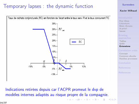
Temporary lapses : the dynamic function

11

notre cadre est celle proposée par l’ACPR dans le cadre de QIS V. Les taux de rachats conjoncturels, fournis par l’ACPR, sont basés sur le positionnement entre le taux servi par l’assureur et le taux attendu (TA) par l’assuré. Le modèle existant ALM développé dans la section III utilise le taux attendu égal au TME comme dans la loi fournie par l'ACPR. En utilisant cette loi, pour une année donnée, le taux de RC se définit de la manière suivante:

°°°°

¯

°°°°

®

t�

��d�

��u

��

��d�

��u

��

G

GJJG

JD

EDED

ED

TATSsiRC

TATSsiTATSRC

TATSsi

TATSsiTATSRC

TATSsiRC

RC

min

min

max

max

0

Avec comme paramètres:

Tableau 2: paramètres loi de rachat conjoncturel proposée par l’ACPR

Par prudence, le plafond min est utilisé dans notre modèle classique ALM.

Le taux de rachat total (RT) s’exprime comme suit:

> @),0(max,1min RCRSRT �

Et la valeur des rachats totaux en montant pour une année donnée s’obtient par la formule suivante:

Indications retirées depuis car l’ACPR promeut le dvp demodèles internes adaptés au risque propre de la compagnie.

14/37

Surrenders

Xavier Milhaud




Conclusion

References

References

Orientations nationales complémentaires du QIS 5

At the end, we consider

LRshocked = min(1,max(0,RS + RC )),

whereRS : structural lapses,RC : temporary lapses (max. is still 30%, so integratesthe mass lapse event as defined previously).

→ Looking at the spread between the contract credited rateand some competitive rate seems to be the right approach.→ Easy to implement for companies.→ However, it still lacks the consideration of potentialcorrelated behaviours in case of financial distress...

15/37

Surrenders

Xavier Milhaud




Conclusion

References

References



3 Correlation crisisUnderlying conceptA first simple common shocks modelAn alternative to model contagion: Hawkes processes


16/37

Surrenders

Xavier Milhaud




Conclusion

References

References

Main idea

A vicious circle can originate from bad economic conditions...

This could lead to big surprise in a Solvency II framework!

Presentation of AXA Global Life / 2010 – V1.0 (2010, june the 29th) The data used in this presentation are the property of AXA Global Life and cannot be reused without the prior written consent of AXA Global Life.

First insight of correlation crisis

Environment

•  Economical situation plays a major role in policyholders’ behaviors

Macroeconomical perturbation

•  Global surrender rate increases as we observe some perturbations on the financial market

Correlation crisis

•  Correlation between insureds significantly increases during crisis or strong recessions [15]

21

Classical modeling of the surrender rate with a Gaussian law (mean and variance observed) becomes erroneous.

Cycle appearing

Lyon - 22/07/2010

17/37

Surrenders

Xavier Milhaud




Conclusion

References

References

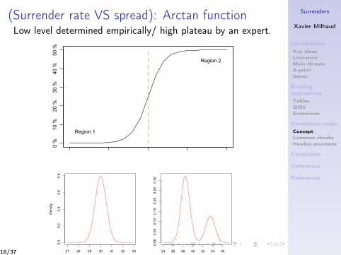
(Surrender rate VS spread): Arctan functionLow level determined empirically/ high plateau by an expert.

Author's personal copy

situation in interest rates markets would lead either to massivesurrenders, or to almost normal lapse rates, depending on politicaldeclarations and on other factors: for example, one of the firstthings that leaders of developed countries said at the beginningof the last crisis was: We guarantee bank deposits and classical sav-ings products. This leads to anticipate policyholders’ behavior morelike a 0 ! 1 law than according to a bell-shaped unimodal distribu-tion. In this paper, we propose a basic model that takes into ac-count correlation crises: as Dr increases, correlation betweenpolicyholders’ decisions increases, and one goes (continuously)from a bell-shaped distribution in the classical regime to a bi-mod-al situation when Dr is large. The model is proposed in Section 1and interpreted in Section 2. In Section 3, we explain how to com-pute surrender rate distributions, with closed formulas and withsimulations. In Section 4, we make use of stochastic orderings inorder to study the impact of correlation on the surrender rate dis-tribution from a qualitative point of view. In Section 5, we quantifythis impact on a real-life portfolio for a global risk managementstrategy based on a Solvency II partial internal model.

1. The model

Assume that when Dr is zero, policyholders behave indepen-dently with average lapse rate l(0), whereas when D r is very large(15%, say), the average lapse rate is 1 ! ! with ! very small, andcorrelation between individual decisions is 1 ! g, with g verysmall. The following model captures these simple features: let Ikbe the random variable that takes value 1 if the kth policyholdersurrenders her contract, and 0 otherwise. Assume that

Ik " JkI0 # $1! Jk%I?k ;

where Jk corresponds to the indicator that the kth policyholder fol-lows the market consensus (copycat behavior). The random variableJk follows a Bernoulli distribution whose parameter p0 is increasingin Dr, and I0; I?1 ; I

?2 . . ., are independent, identically distributed ran-

dom variables, whose parameter p is also increasing in Dr. Thismeans that the surrender probability increases with Dr, and thatthe correlation (Kendall’s s or Spearman q) between Ik and Il (fork– l) is equal to P(Jk = 1jDr = x) when Dr = x, and that in general(without conditioning) the correlation between Ik and Il (for k– l)is equal toZ #1

0P$Jk " 1jDr " x%dFDr$x%:

This is because given that Dr = x, Ik and Il (for k – l) admit a Mardiacopula (linear sum of the independent copula and of Fréchet upperbound).1 For a portfolio of 20000 policyholders, the Gaussianassumption is not too bad for the case where Dr = 0. We show herewith realistic values of the S-shaped curve how this bell-shapedcurve progressively evolves as Dr increases and at some pointDr = x0 becomes bi-modal. McNeil et al. (2005) perfectly illustratesthe problem of correlation risk and its consequences on tail distri-bution in a general context.

2. Interpretation of the model

The S-shaped curve of the surrender rate in function of Dr onFig. 1 shows that the less attractive the contract is, the more thepolicyholder tends to surrender it. Obviously the surrender rateaverage is quite low in a classical economical regime (Region 1,low Dr on Fig. 1), but is significantly increasing as Dr increases. In-deed when interest rates rise, equilibrium premiums decrease and

a newly acquired contract probably provides the same coverage ata lower price: the investor acts as the opportunity to exploit higheryields available on the market. On the contrary, if the interest ratesdrop then the guaranteed credited rate of the contract may be(when it is possible) lowered by the insurer (for financial reasonsor to stimulate the policyholder to surrender).

By consequence, Region 1 in Fig. 1 illustrates the case corre-sponding to independent decisions of policyholders (here the cor-relation tends to 0) whereas Region 2 corresponds to much morecorrelated behaviors (correlation tends to 1 in this situation) be-cause of a crisis for instance. The underlying idea of the paper isthat as long as the economy remains in ‘‘good health’’, the correla-tion between policyholders is quasi nonexistent and thus the sur-render rate (independent individual decisions) can be modeledthanks to the Gaussian distribution whose mean and standarddeviation are those observed. Indeed the suitable distribution inRegion 1 is the classical Normal distribution represented in Fig. 2.

On the contrary the sharp rise of the surrender rate at some le-vel Dr in Fig. 1, followed by a flat plateau which is the maximumreachable surrender rate (this bound is often suggested by an ex-pert since we consider that we have never observed it), reflectsthat economical conditions are deteriorating. The crucial point isto realize that in such a situation the assumption of independentbehaviors can become strongly erroneous: the correlation betweenpolicyholders’ decisions makes the surrender rate distributionchange. This is the consequence of two different behaviors or sce-narios, either almost all policyholders surrender their contract orthey do not. The more suitable distribution to explain it is theso-called Bi-modal distribution illustrated in Fig. 2. The main differ-ence with the Gaussian model is that the average surrender rate re-sults from two peaks of the density.

Note that irrational behavior of policyholders could also lead tocorrelation crises between their decisions even if Dr is small. Weshall see that this situation is the one that has the strongest impacton economic capital needs. Irrational behavior must be understoodhere as atypical with respect to the historical records of the insur-ance company, following some rumor or some recommendationfrom journalists or brokers. From a financial perspective, irrationalbehavior corresponds to the one of policyholders who do not sur-render their contract even if it would pay to surrender it. As lifeinsurance contracts feature more and more complex embeddedoptions or guarantees, and as tax incentives are at stake, it mightbe difficult for the policyholder to use them optimally. However,it can be noticed in the US life insurance market (in which manyvariable annuities are present) that policyholders seem to becomemore and more rational. This uncertainty on future policyholder’srationality is somehow partly captured by our correlation crisismodel.

0 %

10 %

20 %

30 %

40 %

50 %

Region 1

Region 2

Fig. 1. Surrender rate versus Dr.

1 Here the copula of Ik and Il (for k – l) is not unique as their distributions are notcontinuous.

S. Loisel, X. Milhaud / European Journal of Operational Research 214 (2011) 348–357 349

27 28 29 30 31 32 33

0.0

0.2

0.4

0.6

0.8

surrender rate (in %)

Density

24 26 28 30 32 34 36

0.00

0.05

0.10

0.15

0.20

0.25

0.30

surrender rate (in %)

18/37

Surrenders

Xavier Milhaud




Conclusion

References

References

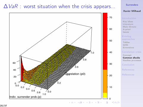
First attempt: a basic mixture model (Region 2)

Common shock model (LM11): Ik = Jk I0 + (1− Jk)I⊥k

Density

surrender rate

30 35 40 45 50 55

0.00

0.05

0.10

0.15

0.20

0.25

0.30

VaR(beta) VaR(alpha)

30 35 40 45 50 55

0.00

0.05

0.10

0.15

0.20

0.25

0.30

VaR(beta)

VaR(alpha)

30 35 40 45 50 55

0.00

0.05

0.10

0.15

0.20

0.25

0.30

surrender rate

Best estimate

Economic capital

Economic capital

Lesson: correlation makes the EC become much higher!However, this is a static model...(does not depend on time t)

19/37

Surrenders

Xavier Milhaud




Conclusion

References

References

∆VaR : worst situation when the crisis appears...

0.00.2

0.40.6

0.81.0

0.0

0.2

0.4

0.6

0.8

1.0

0

20

40

60

Indiv. surrender prob.(p)

Correlation (p0)z

0

10

20

30

40

50

60

70

20/37

Surrenders

Xavier Milhaud




Conclusion

References

References

New approach: Hawkes processes (see (HO74))

Intensity models (almost classical duration models) are alsoused in mortgage prepayments.

Let N = (Nt)t≥0 be a point process with intensity λ = (λt).

N describes the surrenders in an insurance portfolio with anintensity λ following the piecewise deterministic dynamics, i.e.

λt = λ∞ + (λ0 − λ∞)e−βt + α

∫ t

0e−β(t−s)dNs ,

with α, β, λ∞ and λ0 being some positive constants.

→ the surrender intensity is stochastic,→ “internal” source of excitation,→ path-dependent → depends on its history!

21/37

Surrenders

Xavier Milhaud




Conclusion

References

References

Extension : the dynamic contagion process

→ Slightly modified version of Hawkes processes (DZ11).

The mathematical expression for surrender intensity follows

λt = λ∞+(λ0−λ∞)e−βt+α1

∫ t

0e−β(t−s)dNs+α2

∫ t

0e−β(t−s)dN̂s

Notice that the surrender intensity depends on...1 the initial level of surrender intensity λ0,2 λ∞ (for structural surrenders): constant, realistic if the

portfolio composition remains similar over time)...3 endogenous factors: history of Nt → contagion, internal;4 exogenous shocks: history of N̂t → dynamic

dependence, external source of excitation.

22/37

Surrenders

Xavier Milhaud




Conclusion

References

References

23/37

Surrenders

Xavier Milhaud




Conclusion

References

References

Exogenous shocks in our context I

Consider a contract with guaranteed return r ≥ 0 and letr = (rt)t≥0 be the interest rate with GBM dynamics

rt = r0 eXt and Xt = (µ− σ2

2) dt + σWt ,

where µ, σ > 0 and Wt a standard brownian motion.

How the surrender decision is affected by the level of rt?

→ A rational policyholder will surrender as soon as thequantity ∆rt := rt−r

r becomes high enough.

→ Assume that the insurance company incorporates thisfeature in its internal risk model by adjusting the creditedrate r depending on market interest rates level.

24/37

Surrenders

Xavier Milhaud




Conclusion

References

References

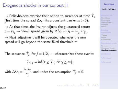
Exogenous shocks in our context II

→ Policyholders exercise their option to surrender at time T̂1(first time the spread ∆rt hits a constant barrier m > 0).

→ At that time, the insurer adjusts the guaranteed returnr = rT̂1

→ “new” spread given by ∆1rt = (rt − rT̂1)/rT̂1

.

→ Next adjustment will be operated whenever the newspread will go beyond the same fixed threshold m.

The sequence T̂j , for j = 1, 2, · · · characterizes these events:

T̂j+1 = inf{t ≥ T̂j , ∆j rt ≥ m},

with ∆j rt =rt−rT̂jrT̂j

and under the assumption T̂0 = 0.

25/37

Surrenders

Xavier Milhaud




Conclusion

References

References

Adjustments of the credited rate

0 20 40 60 80 100

0.014

0.016

0.018

0.020

0.022

0.024

0.026

Interest rate dynamics and adjustments

Time

Inte

rest ra

te v

alu

es

0 20 40 60 80 100

0.014

0.016

0.018

0.020

0.022

0.024

0.026

T̂1 T̂2 T̂3 T̂4 T̂5 T̂6 T̂7T̂8

Interest rateCredited rateJump times

26/37

Surrenders

Xavier Milhaud




Conclusion

References

References

Surrender intensity and counts trajectories0 20 40 60 80 1000.014

0.018

0.022

0.026

Interest rate dynamics and adjustments

Time

Inte

rest

rate

val

ues

0 20 40 60 80 1000.014

0.018

0.022

0.026

T̂1 T̂2 T̂3 T̂4 T̂5 T̂6 T̂7 T̂8

0 20 40 60 80 100

1.0

1.5

2.0

2.5

Dynamic contagion process: intensity process λt

Time

λ t

0 20 40 60 80 100

010

2030

Dynamic contagion process: counting process Nt

Time

Nt

27/37

Surrenders

Xavier Milhaud




Conclusion

References

References

An algorithm for simulating such trajectories

The algorithm that was originally used (but does not work inour case) embeds the following steps:

1 simulate the first internal jump time,2 simulate the first external jump time,3 take the minimum,4 restart at step 1 (from this jump time) to draw the next

one by simulating following interarrival jump times.

Should work for i.i.d. external inter arrival jump times.

28/37

Surrenders

Xavier Milhaud




Conclusion

References

References

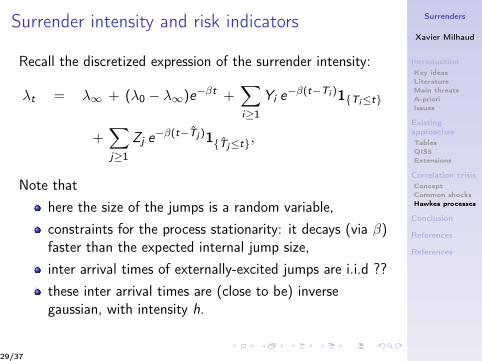
Surrender intensity and risk indicators

Recall the discretized expression of the surrender intensity:

λt = λ∞ + (λ0 − λ∞)e−βt +∑

i≥1Yi e−β(t−Ti )1{Ti≤t}

+∑

j≥1Zj e−β(t−T̂j )1{T̂j≤t},

Note thathere the size of the jumps is a random variable,constraints for the process stationarity: it decays (via β)faster than the expected internal jump size,inter arrival times of externally-excited jumps are i.i.d ??these inter arrival times are (close to be) inversegaussian, with intensity h.

29/37

Surrenders

Xavier Milhaud




Conclusion

References

References

Risk indicators related to the intensityThanks to the piecewise deterministic Markov theory (see(Dav84)), we can derive the expression of the infinitesimalgenerator corresponding to this process.

This leads to (more or less) simple expressions for some keyrisk indicators, such as:

conditional expectation of the intensity

E[λt |λ0] =

(λ0 −

βλ∞β − 1/γ

)e−(β−

1γ )t+

βλ∞β − 1/γ

+1δe−(β−

1γ )t∫ t

0h(s; M, µ, σ) e(β−

1γ )sds,

(1)

(un)conditional variance of the intensity : too long...

unconditional expectation (L = log(1+m)2

σ2 ,M = log(1+m)µ−0.5σ2 ):

E[λt ] =βλ∞

β − 1/γ+

1δ(β − 1/γ)

L2M2 ,

30/37

Surrenders

Xavier Milhaud




Conclusion

References

References

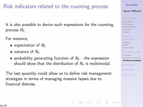
Risk indicators related to the counting process

It is also possible to derive such expressions for the countingprocess Nt .

For instance,expectation of Nt

variance of Nt

probability generating function of Nt : the expressionshould show that the distribution of Nt is multimodal.

The last quantity could allow us to define risk managementstrategies in terms of managing massive lapses due tofinancial distress.

31/37

Surrenders

Xavier Milhaud




Conclusion

References

References

Still to do

What we are now going to look at is:

compare this approach with others (Solvency II,Guru-type model, Gaussian approximations, ...) onseveral key indicators in a (in)finite time horizon:

expectation,variance,probability generating function.

introduce the impacts on some risk measures (VaR,TVaR and others)

assess the corresponding solvency constraints andeconomic capital requirements;

optimization for ORSA purpose.

32/37

Surrenders

Xavier Milhaud




Conclusion

References

References





33/37

Surrenders

Xavier Milhaud




Conclusion

References

References

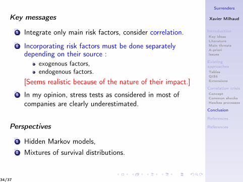
Key messages

1 Integrate only main risk factors, consider correlation.

2 Incorporating risk factors must be done separatelydepending on their source :

exogenous factors,endogenous factors.

[Seems realistic because of the nature of their impact.]

3 In my opinion, stress tests as considered in most ofcompanies are clearly underestimated.

Perspectives

1 Hidden Markov models,2 Mixtures of survival distributions.

34/37

Surrenders

Xavier Milhaud




Conclusion

References

References

Thank you very much for your attention...

...and all comments/questions/ideas are obviously welcome!

35/37

Surrenders

Xavier Milhaud




Conclusion

References

References

References I

[BBP08] A. R. Bacinello, E. Biffis, and Millossovich P., Pricing lifeinsurance contracts with early exercise features, Journal ofComputational and Applied Mathematics (2008).

[CL06] Samuel H. Cox and Yija Lin, Annuity lapse rate modeling: tobitor not tobit?, Society of actuaries, 2006.

[Dav84] Mark HA Davis, Piecewise-deterministic markov processes: Ageneral class of non-diffusion stochastic models, Journal of theRoyal Statistical Society. Series B. Methodological 46 (1984),no. 3, 353–388.

[DZ11] Angelos Dassios and Hongbiao Zhao, A dynamic contagionprocess, Advances in Applied Probability 43 (2011), no. 3,814–846.

[FLP07] Stéphanie Fauvel and Maryse Le Pévédic, Analyse des rachatsd’un portefeuille vie individuelle : Approche théorique etapplication pratique, Master’s thesis, ENSAE, 2007, Mémoire nonconfidentiel - AXA France.

[HO74] Alan G Hawkes and David Oakes, A cluster process representationof a self-exciting process, Journal of Applied Probability (1974),493–503.

[Kag05] Yusho Kagraoka, Modeling insurance surrenders by the negativebinomial model, Working Paper 2005, 2005.

36/37

Surrenders

Xavier Milhaud




Conclusion

References

References

References II[Kim05] Changki Kim, Modeling surrender and lapse rates with economic

variables, North American Actuarial Journal (2005), 56–70.

[Kue05] Siu Tak Kuen, Fair valuation of participating policies withsurrender options and regime switching, Insurance: Mathematicsand Economics 37 (2005), 533–552.

[LM11] Stephane Loisel and Xavier Milhaud, From deterministic tostochastic surrender risk models: Impact of correlation crises oneconomic capital, European Journal of Operational Research 214(2011), no. 2.

[MMDL11] X. Milhaud, V. Maume-Deschamps, and S. Loisel, Surrendertriggers in life insurance: what main features affect the surrenderbehavior in a classical economic context?, Bulletin Francaisd’Actuariat 22 (2011), ?

[Out90] Jean François Outreville, Whole-life insurance lapse rates and theemergency fund hypothesis, Insurance: Mathematics andEconomics 9 (1990), 249–255.

[RH86] A. E. Renshaw and S. Haberman, Statistical analysis of lifeassurance lapses, Journal of the Institute of Actuaries 113 (1986),459–497.

[TKC02] Chenghsien Tsai, Weiyu Kuo, and Wei-Kuang Chen, Earlysurrender and the distribution of policy reserves, Insurance:Mathematics and Economics 31 (2002), 429–445.

37/37

literature mass lapse scenario in insurance, the use of a ... · xavier milhaud introduction key...

Documents