list decoding tensor products and ...prasad/files/tensor...list decoding tensor products and...

LIST DECODING TENSOR PRODUCTS AND INTERLEAVED CODES

PARIKSHIT GOPALAN, VENKATESAN GURUSWAMI, AND PRASAD RAGHAVENDRA

Abstract. We design the first efficient algorithms and prove new combinatorial bounds forlist decoding tensor products of codes and interleaved codes.

• We show that for every code, the ratio of its list decoding radius to its minimum distancestays unchanged under the tensor product operation (rather than squaring, as one mightexpect). This gives the first efficient list decoders and new combinatorial bounds forsome natural codes including multivariate polynomials where the degree in each variableis bounded.

• We show that for every code, its list decoding radius remains unchanged under m-wiseinterleaving for an integer m. This generalizes a recent result of Dinur et al. [7], whoproved such a result for interleaved Hadamard codes (equivalently, linear transforma-tions).

• Using the notion of generalized Hamming weights, we give better list size bounds for bothtensoring and interleaving of binary linear codes. By analyzing the weight distributionof these codes, we reduce the task of bounding the list size to bounding the number ofclose-by low-rank codewords. For decoding linear transformations, using rank-reductiontogether with other ideas, we obtain list size bounds that are tight over small fields.

Our results give better bounds on the list decoding radius than what is obtained fromthe Johnson bound, and yield rather general families of codes decodable beyond the Johnsonradius.

1. Introduction

The decoding problem for error-correcting codes consists of finding the original messagegiven a corrupted version of the codeword encoding it. When the number of errors in thecodeword is too large, and in particular could exceed half the minimum distance of the code,unambiguous recovery of the original codeword is no longer always possible. The notion of listdecoding of error-correcting codes, introduced by Elias [11] and Wozencraft [36], provides oneavenue for error-correction in such high noise regimes. The goal of a list decoding algorithmis to efficiently recover a list of all codewords within a specified Hamming radius of an inputstring. The central problem of list decoding is to identify the radius up to which this goalis tractable, both combinatorially (in terms of the output list being guaranteed to be small,regardless of the input) and algorithmically (in terms of being able to find the list efficiently).

The classical Johnson bound shows that at least combinatorially, list decoding always allowsone to correct errors beyond half the minimum distance. It states that every code over analphabet of size q of fractional minimum distance δ ∈ (0, 1 − 1/q) is list-decodable up to the

Research was supported in part by NSF grants CCF 0343672 and 0953155 and a David and Lucile PackardFellowship.

2 P. GOPALAN, V. GURUSWAMI, AND P. RAGHAVENDRA

(q-ary) Johnson radius

(1.1) Jq(δ)∆=(

1− 1

q

)(

1−√

1− qδ

q − 1

)

which lies in the range (δ/2, δ]. Formally, in such a code, every Hamming ball of fractionalradius ρ = Jq(δ) − γ has at most Oq,δ(1/γ) codewords (i.e., the constant hidden in the O-notation depends on q, δ) [16, Chap. 3]. More precisely, the upper bound of

min δ

2√

1− qδq−1

· 1γ

,δ

γ2

holds on the list-size (the latter bound is at most 1/γ2 which is independent of q, δ and isuseful when δ → 1− 1/q). There is also a version of the Johnson bound that is “alphabet-sizeindependent,” which states that in any code of relative minimum distance at least δ ∈ (0, 1),every Hamming ball of (fractional) radius J(δ) − γ, where

(1.2) J(δ)∆= 1−

√1− δ ,

has at most

(1.3) min δ

2√1− δ

· 1γ

,δ

γ2

codewords.

However, the Johnson bound is oblivious to the structure of the code; it only depends onits minimum distance. Potentially, a code might be list-decodable at larger error-radii thanwhat is guaranteed by the Johnson radius. The question of identifying the precise radius up towhich list decoding is tractable for a family of codes is a challenging problem. Despite muchprogress in designing list decoding algorithms over the last decade, this problem is still openeven for well-studied codes such as Reed-Solomon and Reed-Muller codes.

On the algorithmic side, following the breakthrough results of Goldreich-Levin [12] andSudan [29] which gave list decoders for Hadamard codes and Reed-Solomon codes respectively,there has been tremendous progress in devising list decoders for various codes (see the surveys[16, 17, 30]). This study has had substantial impact on other areas such as complexity theory[31, 33], cryptography [12, 1] and computational learning [20, 22]. Examples of codes whichare known to be list-decodable beyond the Johnson radius have been rare: Extractor codes[32, 15], folded Reed-Solomon codes [25, 18], group homomorphisms [7] and Reed-Muller codesover small fields [13] are the few examples known to us.

A natural way to design new error-correcting codes from old ones is via various productoperations on these codes. In this work, we study the effect of two basic product operations,tensoring and interleaving, on list-decodability. In what follows, [q] stands for an alphabet ofsize q, for example 0, 1, . . . , q − 1.

Definition 1.1. (Tensor Product) Given two linear codes C1 ⊆ [q]n1 and C2 ⊆ [q]n2 , theirtensor product C2⊗C1 consists of all matrices in [q]n2×n1 whose rows belong to C1 and columnsbelong to C2. For a code C ⊆ [q]n, its m-wise tensor product for m > 1 is a code of length nm

defined inductively as C⊗1 = C and C⊗m = C⊗(m−1) ⊗ C for m > 1.

LIST DECODING PRODUCT AND INTERLEAVED CODES 3

For example, Reed-Muller codes inm variables where the degree in each variable is restrictedto d can be viewed as them-wise tensor of Reed-Solomon codes. Our algorithm does not requirethe Cis to be linear, but we make the assumption since the tensor of two non-linear codes mightbe empty. Using δ(C) and R(C) to denote the normalized distance and rate of C respectively,it follows that δ(C⊗m) = δ(C)m and R(C⊗m) = R(C)m. Hence for tensor products, we areprimarily interested in the setting where m is either constant or a slowly growing function ofthe block length.

Definition 1.2. (Interleaved Codes) The m-wise Interleaving (or interleaved product) Cm

of the code C ⊆ [q]n consists of n ×m matrices over [q] whose columns are codewords in C.Each row is treated as a single symbol, thus Cm ⊆ [qm]n.

In other words, under m-wise interleaving, m independent messages are encoded using C,and the m symbols in each position are juxtaposed together into a single symbol over a largeralphabet. For instance, linear transformations from F

n2 → F

m2 can be viewed as interleaved

Hadamard codes. It is easy to see that δ(Cm) = δ(C), R(Cm) = R(C) but the alphabetgrows from [q] to m-dimensional vectors over [q]. So unlike for tensors, for interleaving mcould be as large as polynomial in the block length; indeed our results hold for any m.

1.1. Tensor products and interleaved codes: Prior work and motivation.

1.1.1. Tensoring. Tensor products occupy a central place in coding theory, so much so thattensor product codes are typically referred to as just product codes. Product codes providea convenient way to construct longer codes from shorter component codes. Elias [10] usedtensor product of Hamming codes to construct the first explicit codes with positive rate forcommunication over a binary symmetric channel. The structure of product codes enables de-coding them along columns and rows, and the column decoder can provide valuable reliabilityinformation to the row decoder [27]. Product codes find many uses in practice; for example,the product of two Reed-Solomon codes is used for encoding data on DVDs.

More recently, tensor products have found applications in several areas of theoretical CSsuch as hardness of approximation [9, 2, 21] and constructions of locally testable codes [23].The effect of tensoring on local testability of codes has been extensively studied [3, 8, 35, 5].Tensor products admit a natural tester (which checks a random row/column) that has acertain “robustness” property [3]. Exploiting this, by recursive tensoring one can obtainsimple constructions of locally testable codes with non-trivial parameters, starting from anyreasonable constant-sized code. But to our knowledge, there seems to no prior work focusingon the effect of tensoring on the list decoding radius. In particular, the best combinatorialbound known for the list decoding radius seems to have been the Johnson radius, and we areunaware of an efficient algorithm that decodes C2⊗C1 up to the Johnson radius, assuming thatsuch algorithms exists for each Ci. A sufficiently strong result on list decoding tensor productscould lead to a simple, recursive construction of list-decodable codes starting from any smallcode of good distance. Unfortunately, the results in this paper do not yield sufficiently goodlist size bounds to carry out such a recursive construction of list-decodable codes. The resultsare however optimal in terms of the radius to which they list-decode from.


1.1.2. Interleaving. At a high level, interleaving is a way to arrange data in a non-contiguousway in order to increase performance. Interleaving is used in practical coding systems to grouptogether the symbols of several codewords as a way to guard against burst errors. A bursterror could cause too many errors within one codeword, making it unrecoverable. However,with interleaving, the errors get distributed into a small, correctable number of errors in eachof the interleaved codewords. This is quite important in practice; for example the data in a CDis protected using cross-interleaved Reed-Solomon coding (CIRC). Though code interleavinghas been implicitly studied for its practical importance, our work appears to be the first tostudy it in generality as a formal product operation. We describe some recent theoretical workon interleaved codes which set the stage for our investigation.

The problem of decoding interleaved Reed-Solomon codes from a large number of randomerrors was tackled in [6, 4]. The folded Reed-Solomon codes constructed by Guruswamiand Rudra [18] (which achieve list decoding capacity), and their precursor Parvaresh-Vardycodes [25], are both sub codes of interleaved Reed-Solomon codes, where the m interleavedcodewords are carefully chosen to have dependencies on each other. Dinur et al. in theirwork on list decoding group homomorphisms studied interleaved Hadamard codes, which areessentially all linear transformations from F

nq → F

mq [7]. Their work raised the question of how

the interleaving operation affects the list decoding radius of arbitrary codes, and motivatedour results.

1.2. Brief high-level description of key results. We start with some terminology.The distance dist(C) of a code C ⊆ [q]n is the minimum Hamming distance between twodistinct codewords in C, and its relative distance is defined as dist(C)/n. For a code C of blocklength n and 0 < η < 1, the list-size for radius η, denoted `(C, η), is defined as the maximumnumber of codewords in a Hamming ball of radius ηn. Informally, the list decoding radius(LDR) of C is the largest η such that for every constant ε > 0, the list size for radius (η − ε)is bounded by some function f(q, ε) independent of the block length n.1

Our main result on tensor products is the following: if C has relative distance δ and LDR η,then the list decoding radius of the m-wise product C⊗m is ηδm−1. In other words, the ratioof LDR to relative distance is preserved under tensoring.

For interleaved codes, we prove that the LDR remains unchanged irrespective of the numberof interleaves. In particular, if C has relative distance δ, and Cm is its m-wise interleaving,then for every η < δ one has `(Cm, η) 6 A · `(C, η)B where A,B are constants depending onlyon δ, η and independent of m.

Organization. Formal statement of all the results of this work appear in Section 2. Theseinclude the results described above which apply to arbitrary codes, along with improved listsize bounds for special cases like binary linear codes and transformations. We present ourbounds for interleaved codes in Section 3, and our decoding algorithm for tensor productstogether with its analysis in Section 4. In Section 5, we use the notion of generalized Hammingweights to derive improved list-size bounds for tensor products and interleavings of binarylinear codes. Finally, in Section 6, we show list size bounds for linear transformations that aretight over small fields.

1Here it is implicitly implied that the codes C belong to an infinite family of codes of increasing block length.


2. Our Results

2.1. List decoding tensor products. Given two codes C1 ⊆ [q]n1 and C2 ⊆ [q]n2 , theirtensor product C2⊗C1 consists of all matrices in [q]n2×n1 whose rows belong to C1 and columnsbelong to C2.

We design a generic algorithm that list decodes C2 ⊗C1 using list decoders for C1 and C2 assubroutines, and bound the list-decoding radius by analyzing its performance. Further, if wehave efficient list decoders for C1 and C2, then we get an efficient algorithm for list decodingC2 ⊗ C1. A brief overview of this algorithm is given below in Section 2.1.2. Our main resulton list decoding tensor products is the following.

Theorem 2.1. Let C1 ⊆ [q]n1 and C2 ⊆ [q]n2 be codes of relative distance δ1 and δ2 respectively,and 0 < η1, η2 < 1. Define η∗ = min(δ1η2, δ2η1). Then

`(C2 ⊗ C1, η∗ − ε) 6 eOε(ln `(C1,η1) ln `(C2,η2)) .

In particular, if the LDR of C1, C2 are η1, η2 respectively, then the LDR of C2 ⊗ C1 is at leastη∗.

The decoding radius achieved in Theorem 2.1 is in fact tight: it is easily shown that as-suming that C cannot be list decoded beyond radius η, C⊗2 cannot be list decoded beyondδη (Lemma 4.8). As a corollary, the ratio of the list decoding radius to the relative distancestays unchanged under repeated tensoring.

Corollary 2.2. If C has relative distance δ and list decoding radius η, then the list decodingradius of the m-wise tensor product C⊗m is ηδm−1.

The bounds that we get on list-size for C⊗m are doubly exponential in m. Improving thisbound to singly exponential in m, say exp(O(m)), could have interesting applications, such asa simple construction of list-decodable codes by repeated tensoring, with parameters strongenough for the many complexity-theoretic applications which currently rely crucially on Reed-Solomon list decoding. We are able to obtain some improvements for the case of tensoringbinary linear codes; this is described in Theorem 2.8.

Comparison to the Johnson bound. Even assuming that each of C1 and C2 are decodableonly up to the Johnson radius, Theorem 2.1 gives a bound that is significantly better thanthe Johnson radius, since by convexity Jq(δ1δ2) < min(δ1Jq(δ2), δ2Jq(δ1)) 6 η∗.

2.1.1. Implications for natural codes. Theorem 2.1 gives new bounds on list decoding radiusfor some natural families of codes, which we discuss below.

Reed-Solomon tensors. Let RS[n, k]q denote the Reed Solomon code consisting of eval-uations of degree k polynomials over a set S ⊆ Fq of size n, with distance δ = 1 − k/n.

Such codes are efficiently list-decodable up to the Johnson radius J(δ) = 1−√1− δ using the

Guruswami-Sudan algorithm [19]. The m-wise tensor product of such a RS code is a [nm, km]qcode consisting of evaluations on Sm ⊆ F

mq , of multivariate polynomials in m variables with

individual degree of each variable being at most k. Parvaresh et al. considered the problem ofdecoding these product codes, and extended the Reed-Solomon list decoder to this setting [24].


This yields relatively weak bounds, and as they note, by reducing the problem to decodingReed-Muller codes of order mk, one can do better [26]. Still, these bounds are weaker thanthe Johnson radius J(δm) of the m-wise product, and in fact become trivial when m > n/k.Our results give much stronger bounds, and enable decoding beyond the Johnson radius.

Corollary 2.3. The m-wise tensor of the RS[n, k]q Reed-Solomon code is efficiently list-decodable up to a radius δm−1J(δ)− ε, where δ = 1− k/n is the relative distance of RS[n, k]q,and ε > 0 is arbitrary.

One can compare this with the Johnson radius J(δm) by noting that

δm−1J(δ) = δm(

1

2+

1

4δ +

3

8δ2 + · · ·

)

, J(δm) = δm(

1

2+

1

4δm +

3

8δ2m + · · ·

)

.

Hadamard tensors. Let Had be the [qk, k]q Hadamard code, where a ∈ Fkq is encoded as

the vector a · xx∈Fkq. C is list-decodable up to its relative distance δ = 1− 1/q. The m-wise

tensor product C⊗m consists of all “block-linear” polynomials. Specifically, each codewordin C⊗m is a polynomial P on m × k variables given by x = (x(1), x(2), . . . , x(m)) where each

x(i) = (x(i)1 , . . . , x

(i)k ), such that for each i, P is a linear function in x(i) for each fixing of the

other variables.

Corollary 2.4. The m-wise tensor of [qk, k]q Hadamard codes has list decoding radius equal

to its relative distance(

1− 1q

)m.

This result is interesting in light of a conjecture by Gopalan et al. stating that Reed-Mullercodes of degree m over Fq are list-decodable up to the minimum distance (they proved thisresult for q = 2) [13]. Our result shows m-wise Hadamard tensors which are a natural sub codeof order m Reed-Muller codes (with better distance but lower rate) are indeed list-decodableup to the minimum distance.

2.1.2. Tensor decoder overview. Our algorithm for list decoding C2⊗C1 starts by picking smallrandom subsets S ⊂ [n2] and T ⊂ [n1] of the rows and columns respectively. We assume thatwe are given the codeword restricted to S × T as advice. By alternately running the row andcolumn decoders, we improve the quality of the advice. We show that after four alternations,one can recover the codeword correctly with high probability (over the choice of S and T ).An obstacle in decoding tensor product codes is that some of the rows/columns could havevery high error-rates, and decoding those rows/columns of the received word gives incorrectcodewords. We show that the advice string allows us to identify such rows/columns with goodprobability, thus reducing the problem to decoding from (few) errors and (many) erasures.The scheme of starting with a small advice string and recovering the codeword via a series ofself-correction steps has been used for list decoding Hadamard codes and Reed-Muller codes.Our work is the first (to our knowledge) that applies it outside the setting of algebraic codesdefined over a vector space.

2.2. Interleaved Codes. Armed with a list decoding algorithm for C, a naive attempt atlist decoding Cm would proceed as follows: List decode each column of the received wordseparately to obtain m different lists L1, . . . , Lm, then iterate over all matrices with first


column from L1, second column from L2, etc., and output those close enough to the receivedword. The naive algorithm described above yields the following simple product bound

(2.1) `(C, η) 6 `(Cm, η) 6 `(C, η)m

This upper bound is unsatisfactory since even if `(C, η) = 2, the upper bound on `(Cm, η) is2m. Recent work of Dinur et al. [7] overcame this naive product bound when the codes beinginterleaved arise from group homomorphisms. To this end, they extensively used propertiesof certain set systems that arise in the context of group homomorphisms.

Surprisingly, we show that the product bound can be substantially improved for every codeC. In fact, the list size bound we obtain is independent of the number of interleavings m (asin the above-mentioned results of Dinur et al. [7] ).

Theorem 2.5. Let C be a code of relative distance δ and let η < δ. Define b = d ηδ−η e and

r = dlog δδ−η e. Then, for all integers m > 1, we have

(2.2) `(Cm, η) 6

(

b+ r

r

)

`(C, η)r .

This theorem implies that if C is list-decodable up to radius η, then so is Cm. The conditionη < δ in Theorem 2.5 is necessary, as it can be shown (Lemma 3.7) that `(Cm, δ) > 2m (unlessC is trivial and has only one codeword).

2.2.1. Proof technique. The proof of Theorem 2.5 relies on a simple observation which weoutline below. Assume that we list decode the received word corresponding to the first column,to get a list of candidate codewords for that column and pick one codeword from this list.Rows where the first column of the received word differs from this codeword correspond toerrors, hence we can replace those rows by erasures. Thus for the second column, some ofthe error locations are erased, which makes the decoding easier. Of course, if the codewordis close to the received word, then there may be very few (or no) erasures introduced. Butwe show there are only a few codewords in the list that are very close to the received word.Extending this intuition, we construct a tree of possible codewords for each column and showthat the tree is either shallow or it does not branch too much.

2.3. Better list-size bounds using generalized Hamming weights. For the case ofbinary linear codes, we are able to improve the list size upper bounds for both tensoring andinterleaving (Theorems 2.1 and 2.5 above) using a common technique. We now describe theunderlying idea and the results it yields.

2.3.1. Method overview. Codewords of both interleaved and 2-wise tensor products are natu-rally viewed as matrices. We bring the rank of these matrices into play, and argue that if therank of a codeword is large, then its Hamming weight is substantially higher than the distanceof the code. It turns out that this phenomenon is captured exactly by a well-studied notionin coding theory called generalized Hamming weights (see the survey [34]) that is also closelyrelated to list decoding from erasures [14]. By definition, if the rth-generalized Hammingweight of a code C is δr(C) then in any k-dimensional subspace of C at least δr(C) fraction ofcoordinates are not identically zero. Hence if a codeword of Cm has rank r, then its relative


Hamming weight is at least the rth generalized Hamming weight δr(C) of C. Similarly, rank rcodewords in C ⊗ C have weight at least δr(C)δ(C).

For binary codes, for r large enough, δr(C) approaches 2δ. The Johnson radius of 2δ,J(2δ) = 1 −

√1− 2δ, exceeds δ. Therefore, for r = r(δ, η) large enough, the number of

codewords in a Hamming ball of radius η < δ whose pairwise differences all have rank greaterthan r can be bounded from above using the Johnson bound. Using the deletion argumentfrom [13], the task of bounding the list-size for radius η now reduces to bounding the numberof rank 6 r codewords within radius η. We accomplish this task, for both interleaved andproduct codes, using additional combinatorial ideas. We remark that our use of the deletionargument is more sophisticated than in [13], since most of the work goes into bounding thelist-size for the low-rank case.

We note that the reason the above approach does not work for non-binary alphabets is thatthe generalized Hamming weight δr(C) may not be larger than q

q−1δ for q-ary codes.

2.3.2. Results for interleaved codes. Theorem 2.5 showed that for any code C of distance δ and

for any η < δ, the list-size for the m-wise interleaved code Cm is bounded by `(C, η)dlogδ

δ−ηe.

Note that for η → δ, the exponent grows without bounds. For binary linear codes, using theabove generalized Hamming weights based approach, we can improve this bound to a fixedpolynomial in `(C, η), removing the dependence on log(1/(δ − η)) in the exponent.

Theorem 2.6. For every δ ∈ (0, 1/2), there exists a finite constant dδ > 0 such that for anybinary linear code with distance δ and every η < δ, we have:

`(Cm, η) 6 dδ ·(

`(C, η)δ − η

)dlog 4δe

.(2.3)

Given a binary linear error-correcting code C, the Johnson bound states that the list sizeat radius J2(δ) − ε is bounded by Oδ(1/ε). We can show that essentially the same list-sizebound holds for Cm, provided the distance δ is bounded away from 1

2 .

Theorem 2.7. For every δ, 0 < δ < 12 , there exists a constant cδ such that for every binary

linear code C of relative distance δ,

`(Cm, J2(δ)− ε) 6 cδ/ε .

2.3.3. Result for tensor product. Applying the above approach to the tensor product of twocodes, we prove the following.

Theorem 2.8. Suppose C1 ⊆ Fn12 and C2 ⊆ F

n22 are binary linear codes of relative distance

δ1 and δ2 respectively. Let η1 6 δ1 and η2 6 δ2. Define δ = δ1δ2, η∗ = min(δ1η2, δ2η1) and

r = dlog( 4δ1δ2

)e. Then for some constant bδ that depends only on δ,

`(C2 ⊗ C1, η∗ − ε) 6 bδ`(C1, η1)r`(C2, η2)rε−2r .

Note that the list size is at most a fixed polynomial in the list sizes `(C1, η1) and `(C2, η2)of the original codes, instead of the quasi-polynomial dependence in Theorem 2.1.


2.4. List decoding linear transformations. Let Lin(Fq, k,m) denote the set of all lin-

ear transformations L : Fkq → F

mq . The code Lin(Fq, k,m) is nothing but the m-wise in-

terleaving Hadm(Fq, k) of the Hadamard code Had(Fq, k). Let `(Lin(Fq, k,m), η) denotethe maximum list size for the code Lin(Fq, k,m) at a distance η. Dinur et al. [7] show that`(Lin(F2, k,m), 1/2−ε) 6 O(ε−4) and `(Lin(Fq, k,m), 1−1/q−ε) 6 O(ε−C) for some constantC for general q. The best lower-bound known for any field is Ω(ε−2).

Being a general result for all codes, Theorem 2.5 only gives a quasipolynomial bound for thespecial case of linear transformations. By specializing the above generalized Hamming weightsapproach to the case of linear transformations, and using more sophisticated arguments basedon decoding from erasures for the low-rank case, we prove the following stronger bounds forlist decoding linear transformations over F2.

Theorem 2.9. There is an absolute constant C <∞ such that for all positive integers k,m,

`(

Lin(F2, k,m),1

2− ε)

6 C · ε−2 .

For arbitrary fields Fq, we prove the following bounds, the first is asymptotically tight forsmall fields while the second is independent of q and improves on the bound of Dinur et al. .

Theorem 2.10. There is an absolute constant C ′ <∞ such that for every finite field Fq,

`(

Lin(Fq, k,m), 1 − 1

q− ε)

6 C ′ ·min(q6ε−2, ε−5) .

3. Interleaved Codes

In this section, C ⊂ [q]n will be an arbitrary code (possibly non-linear) over an alphabet [q].We will use `(η) and `m(η) for `(C, η) and `(Cm, η) respectively. Let dq(c1, c2) denote theHamming distance between strings in [q]n and ∆q(c1, c2) = dq(c1, c2)/n denote the normalizedHamming distance. We drop the subscript q when the alphabet is clear from context. Forr ∈ [q]n, B(r, η) ⊂ [q]n denotes the Hamming ball centered at r of radius ηn. We use C forcodewords of Cm and c for codewords of C. We will interchangeably view C as a matrixin [q]n×m and a vector in [qm]n. For a k ×m matrix A, a1, . . . , am will denote its columns,a[1], . . . , a[k] will denote the rows, and A6i will denote the k × i matrix(a1, . . . , ai).

Given an algorithm DecodeC that can list decode C up to radius η, it is easy to give analgorithm DecodeCm that uses DecodeC as a subroutine and runs in time polynomialin the list-size and m; we present this algorithm in Section 3.1. Thus it suffices to boundthe list-size to prove Theorem 2.5. We do this by giving a (possibly inefficient) algorithm,which identifies rows where errors have occurred and erases them. Erasing a set S ⊂ [n] ofco-ordinates is equivalent to puncturing the code by removing those indices. Given r ∈ [q]n,we use r−S to denote its projection on to the co-ordinates in [n] \ S.Definition 3.1. (Erasing a subset) Given a code C ⊆ [q]n, erasing the indices corresponding

to S ⊆ [n] gives the code C−S = c−S : c ∈ C ⊆ [q]n−|S|.

Let |S| = µn. We will only consider the case that µ < δ. It is easy to see that the resultingcode C−S has distance d(C−S) > (δ − µ)n. There is a 1-1 correspondence between codewords


in C and their projections in C−S . For the code C−S , it will be convenient to consider regularHamming distance (not the normalized Hamming distance). For η < 1− µ, let `−S(η) be the

maximum number of codewords of C−S that lie in a Hamming ball of radius ηn in [q]n(1−µ).

Lemma 3.2. For any η < 1− µ, `−S(η) 6 `(η + µ).

Proof. Take a received word r−S ∈ [q]n(1−µ) so that there are L codewords c−S1 , . . . , c−S

L

satisfying d(r−S , c−Si ) 6 ηn. Define r ∈ [q]n by fixing values at the set S arbitrarily. By the

triangle inequality, d(r, ci) 6 (η + µ)n, showing that `(η + µ) > L.

Assume we have a procedure List-Decode that takes as inputs set S ⊆ [n], r ∈ [q]n, anerror parameter e and returns all codewords c ∈ C so that d(c−S , r−S) 6 e (it need not beefficient). We use it to give an algorithm for list decoding Cm, which identifies rows whereerrors have occurred and erases them. Assume we have fixed C6i = (c1, . . . , ci). We erase theset of positions S where C6i 6= R6i and then run a list decoder for C−S on ri+1. The crucialobservation is that since the erased positions all correspond to errors, the number of errorsdrops by |S|. The distance might also drop by |S|, but since η < δ to begin with, this tradeoffworks in our favor.

Algorithm 1. Erase-Decode

Input: R ∈ [qm]n, η.Output: List L of all C ∈ Cm so that ∆qm(R,C) 6 η.

Set S1 = φ, µ1 = 0.For i = 1, . . . ,m1. Set Li = List-Decode(Si, ri, (η − µi)n).2. Choose ci ← Li.3. Set Si+1 = j ∈ [n] s.t. C6i[j] 6= R6i[j]; µi+1 = Si+1/n.Return C = (c1, . . . , cm).

In Step 2, we non-deterministically try all possible choices for ci; the list L is obtainedby taking all possible Cs that might be returned by this algorithm. Also, ci is a codewordin C−Si but we can think of it as a codeword in C by the 1-1 correspondence. Differentchoices for ci lead to different sets Si+1, and hence to different lists Li+1. So the execution ofErase-Decode is best viewed as a tree, we formalize this below.

For a received word R, Tree(R) is a tree with m+ 1 levels. The root is at level 0. A nodev at level i is labeled by C(v) = (c1, . . . , ci). It is associated with a set S(v) ⊆ [n] of erasures

accumulated so far which has size µ(v)n. The resulting code C−S(v) has minimum distance

δ(v)n > (δ − µ(v))n. We find all codewords in C−S(v) that are within distance (η − µ(v))n

of the received word r−S(v)i+1 , call this list L(v). By Lemma 3.2, L(v) contains at most `(η)

codewords. Each edge leaving v is labelled by a distinct codeword ci+1 from L(v); it is assigneda weight w(ci+1) = d(c

−S(v)i+1 , r

−S(v)i+1 )/n. The weight w(c) ∈ [0, 1] of an edge indicates how many

new erasures that edge contributes. Thus µ(v) = w(c1) + · · · + w(ci). The leaves at level mcorrespond to codewords in the list L. There might be no out-edges from v if the list L(v)


is empty. This could result in a leaf node at a level i < m which does not correspond tocodewords. Thus the number of leaves in Tree(R) is an upper bound on the list-size for R.

In order to bound the number of leaves, we assign colors to the various edges based ontheir weights. Let c be an edge leaving the vertex v. We color it White if w(c) < δ − η,

Blue if w(c) > δ − η but w(c) < δ(v)2 and Red if w(c) > δ(v)

2 . White edges correspond tocodewords that are very close to the received word, Blue edges to codewords that are withinthe unique-decoding radius, and Red edges to codewords beyond the unique decoding radius.

We begin by observing that White edges can only occur if the list is of size 1.

Lemma 3.3. If a vertex v has a White out-edge, then it has no other out-edges.

Proof. Assume that the edge labelled with c ∈ L(v) is colored White, so that d(c, r−S(v)i+1 ) <

(δ − η)n. Let c′ be another codeword in L(v), so that d(c′, r−S(v)i+1 ) 6 (η − µ(v))n. Then by

the triangle inequality,

d(c, c′) < (δ − η)n+ (η − µ(v))n = (δ − µ(v))n 6 δ(v)n

But this is a contradiction since d(c, c′) > δ(v)n.

We observe that Blue edges do not cause much branching and cannot result in very deeppaths.

Lemma 3.4. A vertex can have at most one Blue edge leaving it. A path from the root to aleaf can have no more than d η

δ−η e Blue edges.

Proof. The first part holds as there can be at most one codeword within the unique decodingradius. Each Blue edge results in at least (δ − η)n erasures. Therefore, after d η

δ−η e Blue

edges, all ηn errors have been identified, so all remaining edges have to be White.

Lastly, we show that Red edges do not give deep paths either, although a vertex can haveup to `(η) Red edges leaving it.

Lemma 3.5. A path from the root to a leaf can have no more than dlog( δδ−η )e Red edges.

Proof. We claim that every Red edge leaving vertex v has weight at least (δ−µ(v))/2. Indeed,since c is beyond the unique-decoding radius of C−S(v), w(c) > δ(v)

2 , and the relative distance

δ(v) of the code C−S(v) at node v satisfies δ(v) > (δ − µ(v))n.

Assume now for contradiction that some path from the root to a leaf contains k red edgesfor k > dlog( δ

δ−η )e. Suppose that the edges have weights ρ1, . . . , ρk respectively. Contract the

Blue and White edges between successive Red edges into a single edge, whose weight is thesum of weights of the contracted edges. We also do this for the edges before the first Red

edge and those after the last Red edge. This gives a path that contains 2k + 1 edges, wherethe even edges are Red, and the weight of the edges along the path are β1, ρ1, β2, . . . , ρk, βk+1

respectively. Let vi be the parent vertex of the ith Red edge for i ∈ [k]. Then we have


µ(v1) = β1 and µ(vi) = βi + ρi−1 + µ(vi−1) for j > 1. But since ρi−1 > (δ − µ(vi−1))/2 andβi > 0, we get

µ(vi) >δ + µ(vi−1)

2

Now a simple induction on i proves that µ(vi) > δ(1 − 21−i). If we take i = dlog( δδ−η )e + 1,

then

µ(vi) > δ

(

1− δ − η

δ

)

= η.

So when we decode at vertex vi, all the error locations have been identified and erased. Hencewe are now decoding from η < δ erasures and no errors, so the decoding is unique and error-free. So vertex vi will have a single White edge leaving it and no Red edges, which is acontradiction.

Theorem 3.6. Assume η < δ and let b = d ηδ−η e, r = dlog δ

δ−η e. Then Tree(R) has at most(b+r

r

)

`(η)r leaves (and hence `m(η) 6(b+r

r

)

`(η)r).

Proof. We first contract the White edges, since they are the only out-edges leaving theirparent nodes. This gives a tree with only Red and Blue edges. Let t(b, r) denote themaximum number of leaves in a tree where each path has at most b Blue and r Red edges,and each node have have at most one Blue edge and `(η) Red edges leaving it. So we havethe recursion

t(b, r) 6 t(b− 1, r) + `(η)t(b, r − 1)

with the base case t(b, 0) = 1. It is easy to check that t(b, r) 6(

b+rr

)

`(η)r.

We conclude this section by proving that the condition η < δ is necessary.

Lemma 3.7. If code C has relative distance exactly δ, then `m(δ) > 2m.

Proof. Take c1, c2 ∈ C where ∆q(c1, c2) = δ. Now take the received word in Cm to be

R = (c1, . . . , c1). For every T ⊆ [m], let CT to be the codeword where the ith column equalsc1 if i ∈ T and c2 otherwise. It is easy to show that every such codeword is at distance atmost δ from R, showing that `m(δ) > 2m.

3.1. An Efficient Decoding Algorithm for Cm. In this section, we show how thebound on the list size can be used to obtain an efficient list decoding algorithm. Given areceived word R = (r1, . . . , rm), for i 6 m let R6i = (r1, . . . , ri).


Algorithm 2. DecodeCm

Input: R ∈ [qm]n, η.Output: List of all C ∈ Cm so that ∆qm(R,C) 6 η.

1. For i = 1, . . . ,mSet Li = DecodeC(ri, η).2. Set L61 = L1.3. For i = 2, . . . ,mFor C ∈ L6i−1 × Li,Add C to L6i if ∆qm(C,R6i) 6 η.4. Return L6m.

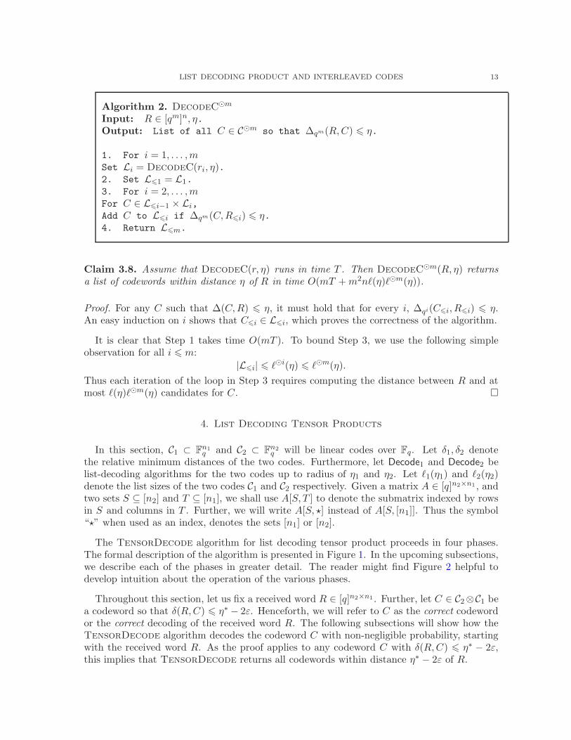
Claim 3.8. Assume that DecodeC(r, η) runs in time T . Then DecodeCm(R, η) returnsa list of codewords within distance η of R in time O(mT +m2n`(η)`m(η)).

Proof. For any C such that ∆(C,R) 6 η, it must hold that for every i, ∆qi(C6i, R6i) 6 η.An easy induction on i shows that C6i ∈ L6i, which proves the correctness of the algorithm.

It is clear that Step 1 takes time O(mT ). To bound Step 3, we use the following simpleobservation for all i 6 m:

|L6i| 6 `i(η) 6 `m(η).

Thus each iteration of the loop in Step 3 requires computing the distance between R and atmost `(η)`m(η) candidates for C.

4. List Decoding Tensor Products

In this section, C1 ⊂ Fn1q and C2 ⊂ F

n2q will be linear codes over Fq. Let δ1, δ2 denote

the relative minimum distances of the two codes. Furthermore, let Decode1 and Decode2 belist-decoding algorithms for the two codes up to radius of η1 and η2. Let `1(η1) and `2(η2)denote the list sizes of the two codes C1 and C2 respectively. Given a matrix A ∈ [q]n2×n1 , andtwo sets S ⊆ [n2] and T ⊆ [n1], we shall use A[S, T ] to denote the submatrix indexed by rowsin S and columns in T . Further, we will write A[S, ?] instead of A[S, [n1]]. Thus the symbol“?” when used as an index, denotes the sets [n1] or [n2].

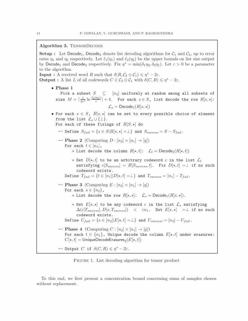
The TensorDecode algorithm for list decoding tensor product proceeds in four phases.The formal description of the algorithm is presented in Figure 1. In the upcoming subsections,we describe each of the phases in greater detail. The reader might find Figure 2 helpful todevelop intuition about the operation of the various phases.

Throughout this section, let us fix a received word R ∈ [q]n2×n1 . Further, let C ∈ C2⊗C1 bea codeword so that δ(R,C) 6 η∗ − 2ε. Henceforth, we will refer to C as the correct codewordor the correct decoding of the received word R. The following subsections will show how theTensorDecode algorithm decodes the codeword C with non-negligible probability, startingwith the received word R. As the proof applies to any codeword C with δ(R,C) 6 η∗ − 2ε,this implies that TensorDecode returns all codewords within distance η∗ − 2ε of R.


Algorithm 3. TensorDecode

Setup : Let Decode1, Decode2 denote list decoding algorithms for C1 and C2, up to errorrates η1 and η2 respectively. Let `1(η1) and `2(η2) be the upper bounds on list size outputby Decode1 and Decode2 respectively. Fix η∗ = min(δ1η2, δ2η1). Let ε > 0 be a parameterto the algorithm.Input : A received word R such that δ(R, C2 ⊗ C1) 6 η∗ − 2ε.Output : A list L of all codewords C ∈ C2 ⊗ C1 with δ(C,R) 6 η∗ − 2ε.

• Phase 1

Pick a subset S ⊆ [n2] uniformly at random among all subsets of

size M = d 12ε2 ln

`2(η2)ε e+ 4. For each s ∈ S, list decode the row R[s, ?]:

Ls = Decode1(R[s, ?])

• For each s ∈ S, B[s, ?] can be set to every possible choice of element

from the list Ls ∪ ⊥.For each of these fixings of B[S, ?] do

-- Define Sfail = s ∈ S|B[s, ?] =⊥ and Ssuccess = S − Sfail.

-- Phase 2 (Computing D : [n2]× [n1]→ [q])For each t ∈ [n1],∗ List decode the column R[?, t]: Lt = Decode2(R[?, t])

∗ Set D[?, t] to be an arbitrary codeword c in the list Ltsatisfying c[Ssuccess] = B[Ssuccess, t]. Fix D[?, t] =⊥ if no such

codeword exists.

Define Tfail = t ∈ [n1]|D[?, t] =⊥ and Tsuccess = [n1]− Tfail.

-- Phase 3 (Computing E : [n2]× [n1]→ [q])For each s ∈ n2,∗ List decode the row R[s, ?]: Ls = Decode1(R[s, ?]).

∗ Set E[s, ?] to be any codeword c in the list Ls satisfying

∆(c[Tsuccess],D[s, Tsuccess]) < εn1. Set E[s, ?] =⊥ if no such

codeword exists.

Define Ufail = s ∈ [n2]|E[?, t] =⊥ and Usuccess = [n2]− Ufail.

-- Phase 4 (Computing C : [n2]× [n1]→ [q])For each t ∈ n1, Unique decode the column E[?, t] under erasures:

C[?, t] = UniqueDecodeErasures2(E[?, t])

-- Output C if δ(C,R) 6 η∗ − 2ε.

Figure 1. List decoding algorithm for tensor product

To this end, we first present a concentration bound concerning sums of samples chosenwithout replacement.


Guess

S

C1(n1, δ1, η1) C1(n1, δ1, η1)

Phase I

B[S, ∗]Ssuccess

Sfail

C2(n2, δ2, η2)

Phase II

D[∗, ∗]

Tfail Tsuccess

Tr TwC1(n1, δ1, η1)

Phase III

Usuccess

Ufail

E[∗, ∗]

C2(n2, δ2, η2)

C2(n2, δ2, η2)

Figure 2. Phases of the TensorDecode Algorithm

Lemma 4.1. Let z1, z2, . . . , zn be real numbers bounded in [0, 1]. Let S ⊆ [n] be a uniformlyrandom subset of size M . Then,

Pr[∣

∣

∣

1

|S|∑

s∈S

zs −1

n

∑

i∈[n]

zi

∣

∣

∣> γ

]

6 p(γ, |S|) = 2e−2γ2M

The above concentration bound essentially a restatement of Corollary 1.1 in Serfling’s work[28] on sums in sampling without replacement. Henceforth, for the sake of succinctness, we

shall use the notation p(γ,M) to denote the upper bound (2e−2γ2M ) in the above lemma.

4.1. Phase 1. In this phase, the goal of the algorithm is to decode a random subset of rowsof the received word R. To this end, the algorithm picks a random subset of rows S, andruns the list decoder Decode1 for the code C1 on each row s ∈ S. On each row s ∈ S, the listdecoder Decode1 could in general return no codeword or a list Ls of up to `1(η1) codewords.


At this stage, the TensorDecode just guesses the correct decoding for each of the rows s ∈ Sfrom the corresponding list Ls ∪ ⊥. More precisely, the algorithm iterates over all possibledecoding of the rows in s ∈ S, from among the lists Ls ∪ ⊥ returned by the algorithmDecode1. Note that for any given row s ∈ S, the algorithm could also guess that the correctdecoding is not part of the list Ls, in which case the guess is ⊥.

To analyze the algorithm, recall that we fixed a correct codeword C that is within distanceη∗ − 2ε from the received word R. Claim 4.2 show that with high probability, (1− δ2 + ε)|S|of the rows are set to the correct codeword from C for some fixing of B[S, ?].

Claim 4.2. With probability at least 1 − p(ε,M) over the choice of the set S, the algorithmiterates over a choice of B[S, ?] such that

|Ssuccess| > (1− δ2 + ε)|S| and B[Ssuccess, ?] = C[Ssuccess, ?]

Proof. Define Sr to be the set of rows in S for which the correct codeword C[s, ?] belongs tothe list Ls, i.e.,

Sr = s|s ∈ S,C[s, ?] ∈ Ls .Let S1 denote the set of rows in S with at most a fraction η1 of errors. Specifically, S1 isdefined as

S1 = s ∈ S|δ(C[s, ?], R[s, ?]) 6 η1 .Observe that for each s ∈ S1, the codeword C[s, ?] will be part of the list Ls, obtained bydecoding the row s. Consequently, we will lower bound the size of Sr by the size of S1. ApplyLemma 4.1 with zi = δ(C[i, ?], R[i, ?]) and the set S. Since δ(C,R) 6 δ2η1−2ε, the averageof the zi is less than or equal to δ2η1 − 2ε. Thus we get

PrS

[

δ(C[S, ?], R[S, ?]) > δ2η1 − ε]

6 p(ε,M) .

Let us suppose δ(C[S, ?], R[S, ?]) < δ2η1−ε. By an averaging argument, less than δ2−ε fractionof the rows C[s, ?]|s ∈ S, the distance δ(C[s, ?], R[s, ?]) > η1, i.e., |S1| > (1 − δ2 + ε)|S|.This immediately implies the lower bound on size of Sr.

Clearly, as the algorithm iterates over all possible choices for B[s, ?], there is some fixingwhere we will have Ssuccess = Sr and Sfail = S − Sr.

4.2. Phase 2. Henceforth, we will assume that Phase 1 is succesful in that B[S, ?] agrees withthe correct codeword for sufficiently many rows s ∈ S. More precisely, let us assume that theassertions of Claim 4.2 holds.

Viewed columnwise, B[S, ?] gives us advice strings for the co-ordinates S of every columncodeword. However, the advice is partial: it is equal to the correct codeword on (1 − δ2 + ε)fraction of co-ordinates within S, and ⊥ on the rest. Fortunately, any two codewords in thecolumn code C2 are distance δ2 apart. Therefore, among all column codewords, the correctcodeword has the maximum agreement with the advice string. Thus the advice B[S, ?] is likelyto identify the correct codeword from a small list of candidates.


In Phase 2, we create a new advice string D[?, ?] by list decoding every column t ∈ [n1], andselecting from the list a codeword that completely agrees with B[S, t] on coordinates where itis not equal to ⊥. If no such codeword exists we set the column to ⊥.

Given that the advice B[S, ?] generated in the first phase is correct codeword on sufficientlymany rows, the following claim suggests that at least (1− δ1 + ε) fraction of columns are cor-rectly decoded to the corresponding columns of C and no more than ε fraction are incorrectlydecoded. In other words, the advice D[?, ?] generated by this phase is a near-sound advicestring with all but a fraction ε of the columns having either the correct value or a failuresymbol ⊥, and further a sizeable fraction of the columns agreeing with the correct codewordC.

Among the columns Tsuccess that are decoded successfully, let Tr, Tw ⊆ Tsuccess denote theset of columns that are decoded correctly and incorrectly respectively. Formally, define setsTr, Tw as follows:

Tr = t ∈ [n1]|D[?, t] = C[?, t] Tw = Tsuccess − Tr

Claim 4.3. Conditioned on the event that the assertions of Claim 4.2 hold, with probabilityat least 1− `2(η2)p(ε,M)/ε over the choice of the set S,

|Tsuccess| > (1− δ1 + 2ε)n1 |Tr| > (1− δ1 + ε)n1 |Tw| < εn1

Proof. Along the lines of the proof of Claim 4.2, let T1 be the set of columns with at most afraction η2 of errors. Formally,

T1 = t ∈ [n1]|δ(C[?, t], R[?, t]) 6 η2By an averaging argument, for at most δ1 − 2ε fraction of the columns C[?, t]|t ∈ [n1], thedistance δ(C[?, t], R[?, t]) > η2, i.e., |T1| > (1− δ1 + 2ε)n1.

Observe that for each column t ∈ T1, the codeword C[?, t] belongs to the list Lt. Conditionedon the assertion of Claim 4.2, B[Ssuccess, ?] = C[Ssuccess, ?]. In particular, the codewordC[?, t] satisfies C[Ssuccess, t] = B[Ssuccess, t]. Consequently, for each t ∈ T1, D[?, t] 6=⊥, i.e.T1 ⊆ Tsuccess. Thus a lower bound on the size of Tsuccess is given by |T1| > (1− δ1 + 2ε)n1.

Now we will upper bound the number of columns that are decoded incorrectly , i.e., |Tw|.Fix a t ∈ [n1]. Let us suppose the tth column is decoded incorrectly, i.e., D[?, t] is neitherequal to ⊥ or C[?, t]. Thus D[?, t] is a codeword in C2 such that

D[Ssuccess, t] = C[Ssuccess, t] .

By the assertion of Claim 4.2,

|Sfail| = |S| − |Ssuccess| < (δ2 − ε)|S| .From the above inequalities, we can conclude

δ(D[S, t], C[S, t]) < δ2 − ε .

Note that D[?, t] and C[?, t] are both codewords of C2 and hence satisfy δ(D[?, t], C[?, t]) = δ2.Since S is a random subset of indices, the distance δ(D[S, t], C[S, t]) is concentrated around δ2.Hence, with very high probability over the choice of S we will have δ(D[S, t], C[S, t]) > δ2− ε.Now, we will apply a union bound over all the codewords in the list Lt to bound the probabilitythat the tth column is decoded incorrectly. The details of the argument are as follows.


Fix a codeword c ∈ Lt such that c 6= C[?, t]. By the distance property of the code C2, wehave δ(c, C[?, t]) > δ2. For each i ∈ [n2], define zi to be 1 if c[i] 6= C[i, t] and 0 otherwise.Applying Lemma 4.1 on the set of real numbers zi and the set S, we get

PrS

[

δ(C[S, t], c[S]) < δ2 − ε]

6 p(ε,M) .

By a union bound over all codewords c ∈ Lt, for a column t ∈ T ,

PrS

[

C[?, t] 6= D[?, t] ∧D[?, t] 6=⊥]

6 `2(η2)p(ε,M) .

In other words, the expected size of Tw is at most `2(η2)p(ε,M)|T |. Applying Markov’sinequality, we get:

PrS

[

∣

∣Tw

∣

∣ > εn1

]

6 `2(η2)p(ε,M)/ε .

To finish the argument, observe that if |Tw| < εn1,

|Tr| = |Tsuccess − Tw| > (1− δ1 + ε)n1 .

Thus with probability 1− `2(η2)p(ε,M)/ε both of the assertions of the claim hold.

4.3. Phase 3. Let us assume that Phase 2 is succesful in that assertions of Claim 4.3 hold.

Viewed row-wise, D gives an advice string for every row. The advice is correct on atleast (1 − δ1 + ε)n1 co-ordinates, wrong on at most εn1 and blank on the rest. The advicethough noisy is sound: since the code C1 has distance δ1n1, a simple application of the triangleinequality shows that there is a unique codeword which disagrees with D[s, ?] on fewer thanεn1 co-ordinates, and that unique codeword is the row C[s, ?]. Thus the advice uniquelyidentifies the correct row codeword.

This phase converts a near sound advice D[?, ?] into a perfectly sound advice E[?, ?] all ofwhose rows are either the correct codewords or the fail symbol ⊥. More precisely, we create anew received word E by list decoding each row of the received word R and using D to identifythe correct codeword in the list, and setting the row to ⊥ if no such codeword exists. Claim4.4 shows this step will find the correct codeword on (1− δ2 + 2ε) fraction of the rows.

Claim 4.4. Conditioned on the event that the assertions of Claim 4.3 hold, for each s ∈Usuccess, E[s, ?] = C[s, ?] and |Usuccess| > (1− δ2 + 2ε)n2.

Proof. By the assertion of Claim 4.3, for each row s ∈ [n2], the codeword C[s, ?] satisfies,

∆(C[s, Tsuccess],D[s, Tsuccess]) = |Tw| < εn1 .

We claim that for each s ∈ [n2], for every codeword c ∈ C2 apart from C[s, ?],

∆(c[Tsuccess],D[s, Tsuccess]) > εn1.

Clearly, this implies that for each row s ∈ Usuccess, we decode the correct codeword, i.e.,E[s, ?] = C[s, ?]. For the sake of contradiction, let us suppose there exists c 6= C[s, ?] satisfying

∆(c[Tsuccess],D[s, Tsuccess]) < εn1.

By triangle inequality, we can conclude

∆(c[Tsuccess], C[s, Tsuccess]) < 2εn1.


Further from claim 4.3, |Tfail| 6 [n1]− |Tsuccess| 6 (δ1 − 2ε)n1. This implies

∆(c, C[s, ?]) < 2εn1 + (δ1 − 2ε)n1 < δ1n1.

This is a contradiction since c and C[s, ?] are two distinct codewords of C1, which is a codewith minimum relative distance δ1.

Let U1 denote the set of rows with less than a fraction η1 of errors; formally,

U1 =

s ∈ [n2]∣

∣

∣δ(C[s, ?], R[s, ?]) 6 η1

.

By an averaging argument, for at most δ2 − 2ε fraction of the rows of C, the distanceδ(C[s, ?], R[s, ?]) > η1, i.e., |U1| > (1− δ2 + 2ε)n2. For each row s ∈ U1, we have C[s, ?] ∈ Ls.From Claim 4.3, for at most εn1 columns in Tsuccess, C[?, t] 6= D[?, t]. Consequently, for eachrow s ∈ U1, E[s, ?] 6=⊥, i.e., U1 ⊆ Usuccess. Hence we get |Usuccess| > |U1| > (1−δ2+2ε)n2.

4.4. Phase 4. When viewed column-wise, E gives the correct value of C on at least a fraction1− δ2+2ε of the coordinates, and is blank on the rest. E[?, ?] is thus a perfectly sound advicewith no incorrect symbols. So now we can completely retrieve the codeword C by decodingeach column from erasures (note that one can uniquely decode C2 from less than a fraction δ2of erasures). Specifically, we make the following claim:

Claim 4.5. Conditioned on the event that the assertions of Claim 4.4 hold, the algorithmTensorDecode outputs the codeword C.

Proof. By Claim 4.4, we know E[s, ?] = C[s, ?] for at least (1−δ2+2ε)n2 rows and E[s, ?] =⊥for the remaining rows. Hence for each column t ∈ [n1], the UniqueDecodeErasures2 algorithmreturns the codeword C[?, t]. Thus the algorithm TensorDecode returns the codewordC.

4.5. Putting the Phases Together. In this section, we will prove the correctness, analyzethe list size output and compute running time of the TensorDecode algorithm.

The following claim is a direct consequence of Claims 4.2, 4.3, 4.4 and 4.5.

Claim 4.6. For a codeword C ∈ C2⊗C1 within distance η∗−2ε of the received word R, the algo-rithm TensorDecode with input R outputs C with probability at least 1−p(ε,M) (1 + `2(η2)/ε)over the choice of S.

Now we will set the parameters appropriately and bound the list size and running time ofthe algorithm.

Theorem 4.7. Given two codes C1, C2, for every ε > 0, the number of codewords of C2 ⊗ C1within distance η∗ = min(δ1η2, δ2η1)− 2ε of any received word is bounded by

4e1ε2

ln `1(η1) ln`2(η2)

ε .

Further, if C1 and C2 can be efficiently list decoded up to error rates η1, η2 and C2 is a linearcode, then C2⊗C1 can be list decoded efficiently up to error rate η∗. Specifically, if T denotes thetime complexity of list decoding C1 and C2, then the running time of the list decoding algorithm

for C2 ⊗ C1 is O(4e1ε2

ln `1(η1) ln`2(η2)

ε × Tn1n2)


Proof. Rewriting the expression for the probability in Claim 4.6 using Lemma 4.1,

1− p(ε,M)

(

1 +`2(η2)

ε

)

= 1− 2e−2ε2M

(

1 +`2(η2)

ε

)

.

Set M = d 12ε2

ln `2(η2)ε e+4. It is easy to see that the probability of success is at least 1

4 with thischoice of parameters. In other words, with this choice of parameters, any codeword C withindistance η∗−2ε is output with probability at least 1

4 . The number of codewords output by thealgorithm is at most the number of possible choices for B[S, ?] from the lists Ls ∪ ⊥s∈S .Thus the algorithm outputs at most (`1(η1) + 1)M codewords, and every codeword C withindistance η∗−2ε is output with probability 1

4 . Hence, the number of codewords within distanceη∗ − 2ε from the received word R is

`(C2 ⊗ C1, η∗ − 2ε) 6 4 (`1(η1) + 1)M 6 4e1ε2

ln `1(η1) ln`2(η2)

ε .

It is easy to check that the running time of the algorithm is as claimed above.

It is easy to show that the list decoding radius reached by TensorDecode is the correct one.

Lemma 4.8. For a linear code C, `(C⊗2, δη) > `(η).

Proof. Let r ∈ [q]n be a received word with codewords c1, . . . , c` ∈ C within radius η. Take c0to be a codeword of minimum weight δ. Define the received word r′ = c0⊗ r. It is easy to seethat the codewords c′i = c0 ⊗ ci for i ∈ [`] are all within distance δη from r′, which proves theclaim.

Thus, if list decoding C beyond radius η is combinatorially intractable, then so is list de-coding C⊗2 beyond radius δη.

Now we shall use the TensorDecode algorithm to obtain list decoding algorithms forrepeated tensors C⊗m of a code C.

Theorem 4.9. Let C be a linear code with distance δ, list decodable up to an error rate η.For every ε > 0, the m-wise tensor product code C⊗m can be list decoded up to an error

rate δm−1η − ε with a list size exp

(

(

Oδ(ln `(η)/ε

ε2))m)

. Furthermore, if C admits an efficient

list decoding algorithm up to radius η, then C⊗m can be efficiently list decoded up to radiusδm−1η − ε.

Proof. Applying Theorem 4.7 with C1 = C2 = C, we get list size bound at error rate δη−3ε forC⊗C. Applying theorem again on C⊗2, we get list size bounds at error rate δ2×(δη−3ε)−3ε =

δ3η − 3δ2ε − 3ε. In general, for C⊗2k let η2k denote the error rate at which we obtain a listsize bound. Then,

η2k = δ2k−1η − 3ε

k−1∑

i=0

δ2i

> δ2k−1η − 3ε

1− δ2.


For brevity, let us denote by Sk the list size `(C⊗2k , η2k). Then from Theorem 4.7, we havethe following recursive inequality:

lnSk+1 61

ε2lnSk (lnSk + ln(1/ε)) .

Set sk = lnSk/ε and a = 1ε2. Then we have the recurrence relation :

sk+1 6 a · s2k s0 = ln`(η)

ε

Thus we get sk 6 (ln `(η)/ε)2ka2

k−1 < (a ln `(η)/ε)2k. Hence we obtain the following list size

bound for m = 2k.

`

(

C⊗m, δm−1η − 3ε

1− δ2

)

6 exp

(

( ln `(η)/ε

ε2

)m)

Rewriting the above expression with ε in place of 3ε1−δ2 ,

`(C⊗m, δm−1η − ε) 6 exp

(

(9 ln 3`(η)/ε(1 − δ2)

(1− δ2)2ε2

)m)

.

The claim about efficiency follows since Theorem 4.7 gives an efficient algorithm for list de-coding C⊗2 based on one for list decoding C. Strictly speaking, in the algorithm for decodingC⊗2 we assumed that the subroutine for decoding C was deterministic and always succeeded,whereas in the inductive steps our algorithms are randomized. This was however only for easeof presentation and is easily handled, for example by amplifying the success probability of therandomized decoders to very close to 1 and then applying a union bound to ensure that allruns are successful with high probability.

5. Improved List-size Bounds via Generalized Hamming Weights

In this section, we prove improved list-size bounds on tensor products and interleavings ofbinary linear codes. This is done by making a connection between the weight-distributions ofsuch codes and the classical coding theoretic notion of Generalized Hamming Weights. Thisallows us to use the Deletion technique of [13] to reduce the problem of bounding list-sizes tothe low-rank case.

We start by introducing the version of the “deletion lemma” that we need. It is a mildlystronger version of the deletion lemma from [13], the graph theoretic view was proposed byImpagliazzo. For convenience, and since this suffices for our applications of this lemma, westate the alphabet-size independent version of the lemma; a similar statement holds for q-arycodes with Jq(µ) replacing J(µ) (for µ 6 1− 1/q).

Lemma 5.1 (Deletion lemma). [13] Let C be a linear code of relative distance δ. Let C′ ⊆ Cbe a (possibly non-linear) subset of codewords so that c′ ∈ C′ iff −c′ ∈ C′, and every codewordc ∈ C \ C′ has wt(c) > µ = µ(δ). Let η = J(µ)− γ for some γ, 0 < γ < 1/2. Then

`(C, η) 6 cδγ· `(C′, η)


for some finite constant cδ depending only on δ.2

Proof. Let r denote a received word, and let L = c1, . . . , ct be the list of all codewords in Cso that ∆(r, ci) 6 η. Construct an (undirected) graph G where V (G) = c1, . . . , ct and (i, j)is an edge if ci − cj ∈ C′. Our goal is to bound |V (G)|.

We claim G does not have large independent sets. Let I = c1, . . . , cs be an independentset. This means that for every i 6= j ∈ [s], ci− cj 6∈ C′ so ∆(ci, cj) > µ. But every codeword inI lies within distance η of r. We now invoke the Johnson bound which states that in a codeof relative distance at least µ, the list-size at radius J(µ)− γ is bounded by c′µ/γ. This shows

that α(G) 6 c′δ/γ.

We claim that the degree of G is bounded by `(C′, η). Suppose that a vertex c has dneighbors c1, . . . , cd. They can be written as c+ c′1, . . . , c+ c′d where c′ ∈ C′. Since

∆(c+ c′i, r) = ∆(c′i, r − c) 6 η

the codewords c′1, . . . , c′d give us a list of codewords in C′ at distance η from the received word

r − c. Hence d 6 `(C′, η).

Thus G has degree d(G) 6 `(C′, η) and the maximum independent set size α(G) 6 c′δ/γ.Thus |V (G)| 6 α(G)(d(G) + 1) 6 cδ

γ · `(C′, η) for some constant cδ <∞.

The deletion lemma is applied in [13] by taking C′ to be all codewords for weight less thanµ, and using `(C′, η) 6 |C′|. However, in our applications |C′| will be too large for this to be auseful bound, thus we essentially use the deletion lemma as a reduction to the low-rank case.

Generalized Hamming Weights (GHWs) arise naturally in the context of list-decoding fromerasures [14]. For a vector v of length n, Supp(v) ⊆ [n] denotes the co-ordinates where vi 6= 0.For a vector space V , Supp(V ) = ∪v∈V Supp(v).

Definition 5.2. The rth generalized Hamming weight of a linear code C ⊆ Fn2 denoted by

δr(C) is defined to be |Supp(Vr)|/n over all r-dimensional subspaces Vr of the code C.

Clearly, δ1(C) = δ(C) is just the minimum distance. The following lower bound on δr(C)which is folklore [16, 34], says that as we consider larger values of r, δr(C) approaches q

q−1δ.

Thus for binary linear codes, δr(C) approaches 2δ(C) as r grows.

Lemma 5.3. For any linear code C ⊆ Fnq with minimum distance δ(C) and any r > 1,

δr(C) >q

q − 1δ(C)

(

1− 1

qr

)

.

Given a matrix C ∈ Fn×mq , let Rank(C) denote its rank, let RowSpan(C) be the space

spanned by its rows and ColSpan(C) be the space spanned by its columns. We use thefollowing standard fact from linear algebra:

2By using the alphabet independent upper bound of 1/γ2 on list-size in the Johnson bound (1.3), we canalso conclude that `(C, η) 6 γ−2

· `(C′, η). This is useful when δ → 1.


Fact 5.4. Given C ∈ Fn×mq such that Rank(C) = r, let 〈v1, . . . , vr〉 be a basis for RowSpan(C).

Then we can write

C =

r∑

s=1

us ⊗ vs

for some vectors u1, . . . , ur which form a basis for ColSpan(C).

5.1. Interleaved Codes. In this subsection C is a binary linear code. We `m(η) to denote`(Cm, η). We use Cm

r to denote the sub-code of Cm consisting of codewords of rank at mostr, and `m

r (η) for `(Cmr , η). The following lemma relates the rank of a codeword to GHWs.

Lemma 5.5. Given C ∈ Cm such that Rank(C) = r, wt(C) > δr(C).

The lemma holds since dim(ColSpan(C)) = r hence its support is at least δr(C). We nowapply the deletion argument to reduce the problem of bounding the list-size to the low-rankcase.

Lemma 5.6. Let C be a binary linear code of relative distance δ and let r = dlog 4δ e. Then

for any η 6 δ, we have`m(η) 6 cδ`

mr (η).

Proof. For r = dlog 4δ e, we have

δr > 2δ(1 − 2−r) > 2δ − δ2/2 .

It is easy to check that

(5.1) J(2δ − δ2/2) = 1−√

1− 2δ + δ2/2 > δ +δ2

4

Let C′ consist of all codewords C where Rank(C) 6 r so that we can take µ = δr in thedeletion lemma. Since J(µ) > δ + δ2/4 whereas η 6 δ, we have

γ = J(µ)− η = (δ − η) +δ2

4>

δ2

4.

Applying the deletion Lemma 5.1, we obtain the desired conclusion

`m(η) 6 c′δγ−1`m

r (η) 6 cδ`mr (η) .

An immediate corollary of Fact 5.4 is

Corollary 5.7. Given a codeword C ∈ Cm of rank r, let b[1], . . . , b[r] be basis for RowSpan(C).Then C can be written as C =

∑rs=1 cs ⊗ b[s] where cs ∈ C for s ∈ [r].

Our goal is to reduce the low-rank problem for interleaved codes to the case when m = r,by fixing a basis for the row-space. The following lemma narrows the choices for the basiselements to rows that have reasonably large weight.

Lemma 5.8. Let ε > 0 and let η = δ − ε. Let C ∈ Cm be a rank r codeword and R be areceived word such that ∆(R,C) 6 η. There is a basis b[1], . . . , b[r] for RowSpan(C) wherewt(C, b[s]) > ε21−r for all s ∈ [r].


Proof. Let

S = b ∈ Span(C) | wt(R, b) > ε21−r, b 6= 0m.We claim that S contains a basis for RowSpan(C), or equivalently dim(S) = r. Assume forcontradiction that dim(S) = r − 1, and that b[1], . . . , b[r − 1] is a basis for it. Complete itto a basis for Span(C) by adding b[r], and let S′ = b[r] + 〈b[1], . . . , b[r − 1]〉. Note that S′ isdisjoint from S.

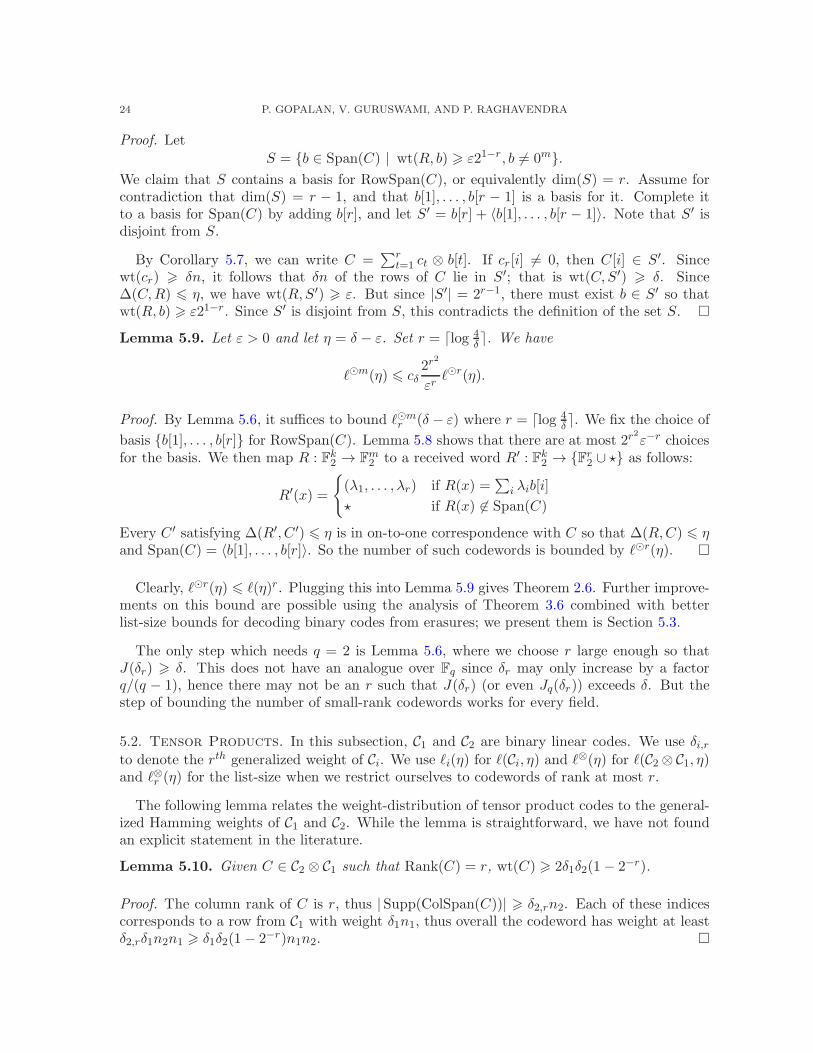
By Corollary 5.7, we can write C =∑r

t=1 ct ⊗ b[t]. If cr[i] 6= 0, then C[i] ∈ S′. Sincewt(cr) > δn, it follows that δn of the rows of C lie in S′; that is wt(C,S′) > δ. Since∆(C,R) 6 η, we have wt(R,S′) > ε. But since |S′| = 2r−1, there must exist b ∈ S′ so thatwt(R, b) > ε21−r. Since S′ is disjoint from S, this contradicts the definition of the set S.

Lemma 5.9. Let ε > 0 and let η = δ − ε. Set r = dlog 4δ e. We have

`m(η) 6 cδ2r

2

εr`r(η).

Proof. By Lemma 5.6, it suffices to bound `mr (δ − ε) where r = dlog 4

δ e. We fix the choice of

basis b[1], . . . , b[r] for RowSpan(C). Lemma 5.8 shows that there are at most 2r2ε−r choices

for the basis. We then map R : Fk2 → F

m2 to a received word R′ : Fk

2 → Fr2 ∪ ? as follows:

R′(x) =

(λ1, . . . , λr) if R(x) =∑

i λib[i]

? if R(x) 6∈ Span(C)

Every C ′ satisfying ∆(R′, C ′) 6 η is in on-to-one correspondence with C so that ∆(R,C) 6 ηand Span(C) = 〈b[1], . . . , b[r]〉. So the number of such codewords is bounded by `r(η).

Clearly, `r(η) 6 `(η)r. Plugging this into Lemma 5.9 gives Theorem 2.6. Further improve-ments on this bound are possible using the analysis of Theorem 3.6 combined with betterlist-size bounds for decoding binary codes from erasures; we present them is Section 5.3.

The only step which needs q = 2 is Lemma 5.6, where we choose r large enough so thatJ(δr) > δ. This does not have an analogue over Fq since δr may only increase by a factorq/(q − 1), hence there may not be an r such that J(δr) (or even Jq(δr)) exceeds δ. But thestep of bounding the number of small-rank codewords works for every field.

5.2. Tensor Products. In this subsection, C1 and C2 are binary linear codes. We use δi,rto denote the rth generalized weight of Ci. We use `i(η) for `(Ci, η) and `⊗(η) for `(C2⊗ C1, η)and `⊗r (η) for the list-size when we restrict ourselves to codewords of rank at most r.

The following lemma relates the weight-distribution of tensor product codes to the general-ized Hamming weights of C1 and C2. While the lemma is straightforward, we have not foundan explicit statement in the literature.

Lemma 5.10. Given C ∈ C2 ⊗ C1 such that Rank(C) = r, wt(C) > 2δ1δ2(1− 2−r).

Proof. The column rank of C is r, thus |Supp(ColSpan(C))| > δ2,rn2. Each of these indicescorresponds to a row from C1 with weight δ1n1, thus overall the codeword has weight at leastδ2,rδ1n2n1 > δ1δ2(1− 2−r)n1n2.


If we let wtr denote the minimum weight of a rank r codeword, we have wtr > 2δ1δ2(1−2−r).We now show a reduction to the low-rank case for tensor products.

Lemma 5.11. Set r = dlog( 4δ1δ2

)e. Then for any η 6 δ1δ2,

`⊗(η) 6 b′δ`⊗r (η) ,

where δ = δ1δ2 and b′δ is a constant depending only on δ.

Proof. Lemma 5.10 shows that for r = dlog( 4δ1δ2

)e any codeword C with Rank(C) = r hasweight at least

wtr = 2δ1δ2(1− 2−r) > 2δ1δ2 − δ21δ22/2.

We apply the deletion lemma taking C′ to be all codewords of rank at most r, with µ =2δ1δ2 − δ21δ

22/2. By Equation (5.1), J(µ) > δ1δ2 + δ21δ

22/4, whereas η 6 δ1δ2. We can take

γ = δ21δ22/4 in the deletion Lemma 5.1, which gives the desired bound.

A corollary of Fact 5.4 for tensor product codes is:

Corollary 5.12. Let C ∈ C2⊗C1 be a codeword of rank r, and let 〈v1, . . . , vr〉 = RowSpan(C).Then C can be written as C =

∑rs=1 us ⊗ vs where 〈u1, . . . , ur〉 = ColSpan(C).

Fix a received word R, which we wish to decode from η? − ε fraction of error where η? =min(η1δ2, η2δ1) and ε > 0. By decoding each row up to radius η1, we get lists L1, . . . ,Ln2 ofcodewords from C1 each of size at most `1(η1). By decoding each column up to radius η2, weget lists L′1, . . . ,L′n1 of codewords from C2 each of size at most `2(η2). The following lemmagives an analogue of Lemma 5.8, restricting the choice of basis vectors to those that occursrelatively frequently among the lists.

Lemma 5.13. Let C ∈ C2 ⊗ C1 be a rank r codeword such that ∆(R,C) 6 η? − ε. There isa basis V = v1, . . . , vr for RowSpan(C) where each vi occurs in at least ε21−rn2 of the listsLi.

Proof. Consider the set of codewords S = v ∈ C1 which occur in the row lists at leastε21−rn2 times. We claim that S contains a basis for RowSpan(C). Assume for contradictionthat it only spans an r − 1 dimensional subspace. Choose v1, . . . , vr−1 which form a basisfor it and complete it to a basis by adding vr. Define the set S′ = vr + 〈v1, . . . , vr−1〉. Now byCorollary 5.12, we can write C in the form C =

∑rs=1 us ⊗ vs for some u1, . . . , ur ∈ S which

span ColSpan(C).

Note that wt(ur) > δ2, hence at least δ2n2 rows (corresponding to indices in the supportof ur) come from the set S′, call this set A ⊂ [n2]. Since the error rate is η? − ε 6 δ2η1 − ε,it must be the case that for some subset B ⊆ A of rows where |B| > εn2, the error rate onthose rows is less than η1; else the overall error rate is at least (δ2 − ε)η1 > δ2η1 − ε > η? − ε.List decoding rows in B up to radius η1 recovers the corresponding row vector from C. So avector from S′ occurs in all lists for rows in B. Hence one of these vectors has to occur withfrequency at least ε21−rn2, but this contradicts the fact that S and S′ are disjoint.

Similarly, let T denote the set of vector u ∈ C2 which occur in in at least ε21−rn1 of thelists L′i. One can show that T contains a basis U = u1, . . . , ur for ColSpan(C).


Lemma 5.14. We have

`⊗r (η? − ε) 6 24r

2ε−2r`1(η1)

r`2(η2)r.

Proof. Note that |S| 6 2r−1`1(η1)ε−1, and |T | 6 2r−1`2(η2)ε

−1. We choose r basis vectorsfrom S and T respectively as bases for RowSpan(C) and ColSpan(C), for which there areat most |S|r|T |r choices. We then choose r row vectors v1, . . . , vr from RowSpan(C) and

r column vectors u1, . . . , ur from ColSpan(C) so that C =∑r

s=1 ui ⊗ vi. This gives 22r2

additional choices. Thus `⊗2 (η? − ε) can be bounded by 22r

2 |S|r|T |r, which gives the desiredbound.

Putting together Lemmas 5.14 and 5.11, we have proved the following theorem.

Theorem 5.15. Let δ = δ1δ2, r = dlog(4δ )e, η2 6 δ1, η2 6 δ2 and η? = min(η1δ2, η2δ1). Thenthere exists a constant bδ so that for any ε > 0.

`⊗(η? − ε) 6 bδ`1(η1)r`2(η2)

rε−2r.

5.3. Further Improvements for Interleaved Codes. Theorem 2.6 was proved by firstreducing to the rank r case for constant r, then reducing to m = r by fixing a basis, andusing the trivial upper bound `r(η) 6 `(η)r. One can improve on this last bound using theanalysis of Theorem 3.6 combined with better list-size bounds for decoding binary codes fromerasures.

Theorem 5.16. For any binary linear code C of relative distance δ, let r = dlog 4δ e. For any

η < δ

`m(η) 622r

2

δ4(δ − η)r

r−1∏

k=0

`

(

η − δ(1 − 2−k)

2

)

(5.2)

For a binary error correcting code with relative distance δ and µ 6 η < δ, we let `′(µ, η−µ)denote the list-size for C with µ erasures and η − µ errors.

Lemma 5.17. For any µ 6 η, we have

`′(µ, η − µ) 6 2 · `(η − µ/2).

Proof. Let r ∈ 0, 1, ?n be a received word where wt(r, ?) > µ. Let L = c1, · · · , ck denoteall codewords of C that satisfy ∆(ci, r) 6 η. Set the erased positions of r at random in 0, 1,call this received word r′. Then Pr[∆(r′, ci) 6 η − µ/2] > 1

2 . Thus, in expectation over thesettings of the erased bits, k/2 of the codewords from L satisfy ∆(r′, ci) 6 η − µ/2. Fixingone such choice of r:

`′(µ, η − µ)

26 `(η − µ/2).

The following lemma completes the proof of Theorem 5.16.


Lemma 5.18. Let C be a binary code with distance δ. Then for any η < δ we have

`r(η) 6 r2rr−1∏

k=0

`

(

η − δ(1 − 2−k)

2

)

.(5.3)

Proof. We run Algorithm 1 on the received word R and build a tree. We mark each edgeleaving v Blue if it lies within the unique-decoding radius (for the code being decoded atv) and Red otherwise. A simple induction shows that after k Red edges, we have at leastδ(1− 2−k) erasures. Thus, after k Red edges, the degree of the tree drops to

`′(η, δ(1 − 2−k)) 6 2`

(

η − δ(1 − 2−k)

2

)

.

Solving the recursion for the number of leaves shows that

`r(η) 6 r2rr−1∏

k=0

`

(

η − δ(1 − 2−k)

2

)

.

Equation 5.3 allows us to replace `(η)r term in Equation 2.3 with the product `(η)`(η −δ/4)`(η − 3δ/8) · · · . This advantage is pronounced if the list size decreases rapidly as theradius shrinks; which happens if we use the Johnson bound to bound the list-size. We finishthe proof of Theorem 2.7.

Proof of Theorem 2.7.Set η = J2(δ)− ε. Note that δ − η > δ − J2(δ). Let r = dlog 4

δ e. Using Lemma 5.9, we get

`m(J2(δ) − ε) 6 c′′δ2r

2

(δ − J2(δ))r· `r(J2(δ) − ε) = c′δ · `r(J2(δ)− ε) ,(5.4)

for some constant c′δ that only depends on δ < 1/2. Applying Lemma 5.18, we conclude that

`r(J2(δ) − ε) 6 r2rr−1∏

k=0

`(

J2(δ) − γk)

,

where γk = δ(1−2−k)2 + ε. The Johnson bound states that `(J2(δ) − γ) 6 Oδ(1/γ). For k > 1,

we can lower bound γk by δ(1−2−k)2 . Hence we have

`r(J2(δ) − ε) 6 r2r ·Oδ(1/ε) ·r−1∏

k=1

4

δ2(1− 2−k)26

cδε

.(5.5)

Combining Equations 5.4 and 5.5 gives the desired result.


6. List Decoding Linear Transformations

In the previous sections, we have developed techniques for decoding generic interleavedcodes based on generalized Hamming weights and decoding from erasures. These can beapplied to get sharper bounds for specific families of codes. We illustrate this in the case oflinear transformations.

The problem of list decoding linear transformations is equivalent to list decoding interleavedHadamard codes. Equivalently, one can think of the message as a matrix M over Fq of

dimension k×m, encoded by the values xtM for every x ∈ Fkq . Thus the encoding is a matrix

C of dimension qk ×m where each column is a codeword in the Hadamard code. Recall thewell known list size bound `(1− 1

q − ε) 6 O(ε−2) for Hadamard codes over Fq.

Consider the space Lin(Fq, k,m) of all linear transformations L : Fkq → F

mq . We use

`m(Hadq, η) instead of to denote the denote the list-size for Lin(Fq, k,m) at distance η.We let Linr(Fq, k,m) denote the space of all linear transformations of rank at most r inLin(Fq, k,m) and let `m

r (Hadq, η) denote the list-size for Linr(Fq, k,m).

6.1. Linear Transformations over F2. We first use the deletion lemma to reduce thetask of proving list-size bounds for Lin(F2, k,m) to that of proving bounds for Lin2(F2, k,m).In this subsection, we use `m(η) to denote `m(Had2, η) and `m

r (η) to denote `mr (Had2, η).

Lemma 6.1. For any η < 1/2, we have `m(η) 6 C`m2 (η) where C is an absolute constant.

Proof. We take C′ to consist of all linear transformations of rank at most 2. Thus for anycodeword L 6∈ C′, Rank(L) > 3, hence wt(L) > 7

8 , so we take µ = 78 . Since J(7/8) > 0.65 and

η < 12 , we can apply the deletion lemma with γ = 0.15 to conclude that `m(η) 6 C`m

2 (η).

To bound `m2 (η), we start by bounding `m

1 (η), which is the maximum number of rank 1linear transformations within distance η of the received word R. We need some facts about thestructure of L(x) when L is a linear transformation of rank r. Recall that we use l[1], . . . , l[k] ∈Fm2 for the rows of L, thought of as vectors from F

m2 . Let RowSpan(L) ⊆ F

m2 denote the r-

dimensional space spanned by these vectors. We write RowSpan(L) = 〈l′[1], . . . , l′[r]〉 todenote the fact that l′[1], . . . , l′[r] form a basis for RowSpan(L). For a function r : Fk

2 → Fm2

and a vector v ∈ Fm2 , we define wt(R, v) = Prx[R(x) = v].

Lemma 6.2. For L ∈ Linr(F2, k,m) and any v ∈ RowSpan(L), wt(L, v) = 2−r.

Proof. The jth column of L defines a linear function lj(x) = xtlj from Fk2 → F2. We

have L(x) = (l1(x), . . . , lt(x)). Let us pick a basis for the columns, assume that this ba-sis is l1, . . . , lr. Let v6r denote the projection of v onto the first r co-ordinates. We havePrx[(l1(x), . . . , lr(x)) = v6r] = 2−r, which implies the claim.

6.1.1. Bounding rank 1 linear transformations. The above lemma implies, in particular, thatif Rank(L) = 1 and RowSpan(L) = 〈l′[1]〉, then wt(L, l′[1]) = wt(L, 0k) = 1

2 .

Corollary 6.3. Let L ∈ Lin1(F2, k,m) and R : Fk2 → F

m2 be such that ∆(R,L) 6 1

2 − ε. IfRowSpan(L) = 〈l′[1]〉, then wt(R, l′[1]) > ε.


This narrows the choice of basis vectors for RowSpan(L) to at most 1ε vectors where

wt(L, l′[1]) > ε. Once we fix l′[1], the problem reduces to Hadamard decoding (or ratherm = 1). Given R : Fk

2 → Fm2 , we define r : Fk

2 → F2 ∪ ? as follows:

r(x) =

0 if R(x) = 0m,

1 if R(x) = l′[1],

? otherwise.

Setting r(x) = ? denotes an erasure; since R(x) 6∈ RowSpan(L), we know there is an error atindex x. Given a Hadamard codeword l : Fk

2 → F2, if we define L ∈ Lin1(F2, k,m) by reversingthe substitution:

L(x) =

l′[1] if l(x) = 1,

0m if l(x) = 0

then it follows that ∆(R,L) = ∆(r, l). This proves the following claim.

Lemma 6.4. The linear transformations L ∈ Lin1(F2, k,m) so that ∆(R,L) < 12 − ε and

RowSpan(L) = 〈l′[1]〉 are in one-to-one correspondence with Hadamard codewords l so that∆(r, l) < 1

2 − ε.

Since there can be at most O( 1ε2 ) codewords of the Hadamard code within distance 1

2 − ε,

and at most 1ε choices for l′[1], this suffices to prove a bound of O( 1

ε3). We can improve this

to O( 1ε2) by observing that if there are many choices for l′[1], then each of them is likely to

result in fewer codewords. This relies on the following Lemma about Hadamard decoding witherasures.

Lemma 6.5. Given r : Fk2 → F2 ∪ ? so that wt(R, ?) > η, the number of codewords l such

that ∆(r, l) < ε is bounded by 2(η+2ε)2 .

Proof. We use the well known fact that the number of codewords so that ∆(r, l) < 12 − ε is

bounded by 14ε2

. So assume there are s codewords l1, . . . , ls. Consider setting each erasure to

a random value in F2. For any l, with probability 12 we have ∆(r, l) 6 1

2 −η2 − ε. Thus in

expectation, s2 of the codewords will now satisfy ∆(l, r) < 1

2 −η2 − ε. Fix one such setting of

the erasures. But now we haves

26

1

(η + 2ε)2⇒ s 6

2

(η + 2ε)2.

We can now show an O(ε−2) bound on rank 1 transformations.

Lemma 6.6. For any ε > 0, we have

`m1 (

1

2− ε) 6

1

2ε2.

Proof. Assume that the condition wt(R, l′) > ε holds for t non-zero row vectors l′ ∈ Fm2 . Fix

one such choice of l′. We then erase η > (t − 1)ε positions, so by Lemma 6.5 the number ofcandidates is no more than 2

(t+1)2ε2 . Thus overall the list-size is bounded by 2t(t+1)2ε2 6 1

2ε2 .


6.1.2. Bounding rank 2 linear transformations. We now proceed to analyzing the list-size forrank 2 linear transformations. We begin with the analog of Corollary 6.3 for the rank twocase.

Corollary 6.7. Let L ∈ Lin2(F2, k,m) and R : Fk2 → F

m2 be such that ∆(R,L) 6 1

2 −ε. Thereis a basis u, v for RowSpan(L) such that wt(R,u) and wt(R, v) are both at least ε

2 .

Proof. Note that wt(L, l[1]),wt(L, l[2]) and wt(L, l[1] + l[2]) are all exactly 14 . If two of the

symbols l[1], l[2], l[1]+l[2] have weight less than ε2 in R, then ∆(R,L) > 2(14− ε

2 ) =12−ε.

In fact, we can assume that wt(R,u) > 112 and wt(R, v) > ε

2 , but we will not use this claim.

Once we pick u and v we reduce to the case m = 2 by defining r : Fk2 → F2

2 ∪ ? as follows:

r(x) =

(λ, µ) if R(x) = λu+ µv,

? otherwise.

We have the following analogue of Lemma 6.4.

Lemma 6.8. The linear transformations L ∈ Lin2(F2, k,m) so that ∆(L,R) < 12 − ε are in

one-to-one correspondence with linear transformations l ∈ Lin2(F2, k, 2) so that ∆(l, r) < 12−ε.

Lemma 6.9. Let r : Fk2 → F2

2 ∪ ? be such that wt(r, ?) > η. The number of linear transfor-mations l ∈ Lin2(F2, k, 2) so that ∆(l, r) < 1

2 − ε is bounded by 100(η+2ε)2

.

Proof. Let l = (l1, l2) where each li : Fk2 → F2. We proceed as in Theorem 2.5, erasing errors

whenever they are located. We run Hadamard decoding on the first column which gives a listL1 of 2

(η+2ε)2candidates for `1. We then choose c ∈ L1, erase the positions where it differs

from R and list decode the resulting word to get candidates for l2.

At most one codeword c ∈ L1 can have error rate less than 14 . If we choose l1 = c, we have

no more than 2(η+2ε)2 choices for the second column. The other codewords in L1 which are

beyond distance 14 result in η > 1

4 erasures, hence a list-size of C 6 32 for the second column.So the overall list size is bounded by

1 · 2

(η + 2ε)2+

2

(η + 2ε)2· 32 6

100

(η + 2ε)2.

We are now ready to bound the number of rank 2 transformations.

Lemma 6.10. There is a constant C ′ so that for any ε > 0, we have

`m2 (

1

2− ε) 6

C ′

ε2.

Proof. Assume there are t > 2 non-zero vectors v ∈ Fm2 so that wt(v) > ε

2 . By Corollary 6.7,each there is a basis u, v of L where wt(R,u) and wt(R, v) are both at least ε

2 . Once we fixthis basis, we erase all positions containing vectors other than u, v and u+ v. This results in


η > (t − 3)ε erasures. Thus by Lemma 6.9, the number of L such that RowSpan(L) = 〈u, v〉is bounded by

100

(η + 2ε)26

100

(t− 1)2ε2.

Since there are(t2

)

choices for u, v, we get an overall bound of(

t

2

)

· 100

(t− 1)2ε2=

t

2(t− 1)

100

ε26

100

ε2

If there are t < 2 nonzero vectors v ∈ Fm2 with wt(v) > ε

2 , then it corresponds to the rank one

case. Thus, adding bounds for rank 1 and rank 2 cases, we have `m2 (12 − ε) 6 100

ε2+ 1

2ε2=

C′

ε2.

6.1.3. Final list-size bound. Combining Lemma 6.10 with Lemma 6.1, we conclude that forsome absolute constant C > 0,

`m(1

2− ε) 6

C

ε2,

thus completing the proof of Theorem 2.9.

6.2. Linear Transformations over Fq. In this subsection, we use `m(η) to denote`m(Hadq, η) and `m

r (η) to denote `mr (Hadq, η). One can repeat the above proof of Theorem

2.9 from the previous subsection for any Fq, and show that for some absolute constant c,

`m(Hadq, 1− 1/q − ε) 6cq6

ε2.

This gives an asymptotically tight bound for constant q. In this subsection, our goal will beto remove the dependence on q. We will do so at the expense of a worse dependence (of ε−5)of the bound on ε.

We begin with a deletion argument analogous to Lemma 6.1. The difference is that weonly delete rank 1 transformations, and the multiplicative overhead is O(ε−2) as opposed toan absolute constant.

Lemma 6.11. For η = q−1q − ε, we have `m(η) 6 C

ε2 `m1 (η).

Proof. We take C′ to consist of all linear transformations of rank at most 1. So we can takeµ = 1− 1

q2(so that J(µ) = 1− 1

q ) and then apply the deletion Lemma 5.1 for this choice of µ and

η = ε. Together with the alphabet independent list-size upper bound (1.3) of 1/ε2 at radiusJ(µ)− ε (see the footnote to Lemma 5.1), this lets us conclude that `m(η) 6 1

ε2`m1 (η).

Given v ∈ Fmq we now define wt(R, v) =

∑

µ∈F?qPrx∈Fm

q[R(x) = µv]. We have the following

q-ary analogue of Corollary 6.7.

Corollary 6.12. Let L ∈ Lin1(Fq, k,m) and R : Fkq → F

mq be such that ∆(R,L) 6 1− 1

q − ε.

If RowSpan(L) = 〈v〉 then wt(R, v) > ε.


Fixing the vector v (from amongst t 6 1ε choices), reduces the problem to Hadamard

decoding over Fq. For Hadamard codes, the list-size at radius 1 − 1q − ε is bounded by 1

ε2 .

This gives the following bound.

Lemma 6.13. For any ε > 0 we have `m1

(

1− 1q − ε

)

6 1ε3 .

Plugging this into Lemma 6.11 completes the proof of Theorem 2.10.

References

[1] A. Akavia, S. Goldwasser, and S. Safra. Proving hard-core predicates using list decoding. In Proc. 44th

IEEE Symposium on Foundations of Computer Science (FOCS’03), pages 146–155, 2003.[2] S. Arora, L. Babai, J. Stern and Z. Sweedyk. The Hardness of Approximate Optima in Lattices, Codes,

and Systems of Linear Equations. Journal of Computer and System Sciences, 54(2):317–331, 1997.[3] E. Ben-Sasson and M. Sudan. Robust locally testable codes and products of codes. Random Struct. Algo-

rithms, 28(4):387–402, 2006.[4] D. Bleichenbacher, A. Kiayias, and M. Yung. Decoding interleaved Reed-Solomon codes over noisy chan-

nels. Theoretical Computer Science, 379(3):348–360, 2007.[5] D. Coppersmith and A. Rudra. On the robust testability of product of codes. Technical Report (104),

Electronic Colloquium on Computational Complexity (ECCC), 2005.[6] D. Coppersmith and M. Sudan. Reconstructing curves in three (and higher) dimensional space from noisy

data. In Proc. 35th ACM Symposium on Theory of Computing (STOC’03), pages 136–142, 2003.[7] I. Dinur, E. Grigorescu, S. Kopparty, and M. Sudan. Decodability of group homomorphisms beyond the

Johnson bound. In Proc. 40th ACM Symposium on Theory of Computing (STOC’08), pages 275–284, 2008.[8] I. Dinur, M. Sudan, and A. Wigderson. Robust local testability of tensor products of LDPC codes. In

APPROX-RANDOM’06, pages 304–315, 2006.[9] I. Dumer, D. Micciancio, and M. Sudan. Hardness of approximating the minimum distance of a linear

code. IEEE Transactions on Information Theory, pages 22–37, (2003).[10] P. Elias. Error-free coding. IEEE Transactions on Information Theory, 4(4):29–37, 1954.[11] P. Elias. List decoding for noisy channels. Technical Report 335, Research Laboratory of Electronics, MIT,

1957.[12] O. Goldreich and L. Levin. A hard-core predicate for all one-way functions. In Proc. 21st ACM Symposium

on the Theory of Computing (STOC’89), pages 25–32, 1989.[13] P. Gopalan, A. Klivans, and D. Zuckerman. List-decoding Reed-Muller codes over small fields. In Proc.

40th ACM Symposium on Theory of Computing (STOC’08), pages 265–274, 2008.[14] V. Guruswami. List decoding from erasures: bounds and code constructions. IEEE Transactions on In-

formation Theory, 49(11):2826–2833, 2003.[15] V. Guruswami. Better extractors for better codes? In Proceedings of the 36th Annual ACM Symposium

on Theory of Computing (STOC’04), pages 436–444, 2004.[16] V. Guruswami. List Decoding of Error-Correcting Codes, volume 3282 of Lecture Notes in Computer Sci-

ence. Springer, 2004.[17] V. Guruswami. Algorithmic Results in List Decoding, volume 2 of Foundations and Trends in Theoretical

Computer Science. Now Publishers, 2006.[18] V. Guruswami and A. Rudra. Explicit codes achieving list decoding capacity: Error-correction with optimal

redundancy. IEEE Transactions on Information Theory, 54(1):135–150, 2008.[19] V. Guruswami and M. Sudan. Improved decoding of Reed-Solomon and Algebraic-Geometric codes. IEEE

Transactions on Information Theory, 45(6):1757–1767, 1999.[20] J. Jackson. An efficient membership-query algorithm for learning DNF with respect to the uniform distri-

bution. Journal of Computer and System Sciences, 55:414–440, 1997.[21] S. Khot. Hardness of approximating the shortest vector problem in lattices. Journal of the ACM, 52(5):789–

808, 2005.[22] Y. Mansour. Learning Boolean functions via the Fourier transform. Theoretical Advances in Neural Com-

putation and Learning, pages 391–424, 1994.


[23] O. Meir. Combinatorial construction of locally testable codes. In Proc. 40th ACM Symposium on Theoryof Computing (STOC’08), pages 285–294, 2008.

[24] F. Parvaresh, M. El-Khamy, M. Stepanov, D. Augot, R. J. McEliece, and A. Vardy. Algebraic list decodingof Reed-Solomon product codes. In Proceedings of the Tenth International Workshop on Algebraic andCombinatorial Coding Theory, Zvenigorod, Russia, pages 210–213, September 2006.

[25] F. Parvaresh and A. Vardy. Correcting errors beyond the Guruswami-Sudan radius in polynomial time. InProceedings of the 46th IEEE Symp. on Foundations of Computer Science, pages 285–294, 2005.

[26] R. Pellikaan and X.-W. Wu. List decoding of q-ary Reed-Muller codes. IEEE Transactions on InformationTheory, 50(4):679–682, 2004.

[27] S. Reddy and J. P. Robinson. Random error and burst correction by iterated code. IEEE Transactions onInformation Theory, 18(1):182–185, 1972.

[28] R.J.Serfling. Probability inequalities for the sum in sampling without replacement. Annals of Statistics,2(1):39–48, (1974).

[29] M. Sudan. Decoding of Reed-Solomon codes beyond the error-correction bound. Journal of Complexity,13(1):180–193, 1997.

[30] M. Sudan. List decoding: Algorithms and applications. SIGACT News, 31(1):16–27, 2000.[31] M. Sudan, L. Trevisan, and S. P. Vadhan. Pseudorandom generators without the XOR lemma. J. Comput.

Syst. Sci., 62(2):236–266, 2001.[32] A. Ta-Shma and D. Zuckerman. Extractor codes. IEEE Transactions on Information Theory, 50(12):3015–

3025, 2004.[33] L. Trevisan. List-decoding using the XOR lemma. In Proc. 44th IEEE Symposium on Foundations of

Computer Science (FOCS’03), pages 126–135, 2003.[34] M. A. Tsfasman and S. G. Vladut. Goemetric approach to higher weights. IEEE Transactions on Infor-

mation Theory, 41:1564–1588, 1995.[35] P. Valiant. The tensor product of two codes is not necessarily robustly testable. In APPROX-RANDOM’05,

pages 472–481, 2005.[36] J. Wozencraft. List decoding. Technical Report 48:90-95, Quarterly Progress Report, Research Laboratory

of Electronics, MIT, 1958.

Microsoft Research Silicon Valley, Mountain View, CA. Some of this work was done when

the author was a postdoc at the University of Washington visiting Princeton University.

E-mail address: [email protected]

Computer Science Department, Carnegie Mellon University, Pittsburgh, PA. Some of this

work was done when the author was a member in the School of Mathematics, Institute for

Advanced Study.


College of Computing, Georgia Institute of Technology, Atlanta, GA. Some of this work

was done while at the University of Washington and visiting Princeton University.


list decoding tensor products and ...prasad/files/tensor...list decoding tensor products and...

Documents