linear regression problems - department of statisticswinner/sta6166/linear_regression.pdf ·...

Linear Regression Problems

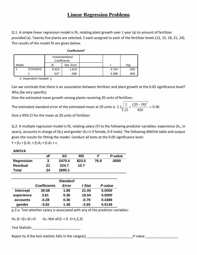
Q.1. A simple linear regression model is fit, relating plant growth over 1 year (y) to amount of fertilizer

provided (x). Twenty five plants are selected, 5 each assigned to each of the fertilizer levels (12, 15, 18, 21, 24).

The results of the model fit are given below:

Can we conclude that there is an association between fertilizer and plant growth at the 0.05 significance level?

Why (be very specific).

Give the estimated mean growth among plants receiving 20 units of fertilizer.

The estimated standard error of the estimated mean at 20 units is 46.0450

)1820(

25

11.2

2

Give a 95% CI for the mean at 20 units of fertilizer.

Q.2. A multiple regression model is fit, relating salary (Y) to the following predictor variables: experience (X1, in

years), accounts in charge of (X2) and gender (X3=1 if female, 0 if male). The following ANOVA table and output

gives the results for fitting the model. Conduct all tests at the 0.05 significance level:

Y = 0 + 1X1 + 2X2 + 3X3 +

ANOVA

df SS MS F P-value

Regression 3 2470.4 823.5 76.9 .0000

Residual 21 224.7 10.7

Total 24 2695.1

Coefficients

Standard

Error t Stat P-value

Intercept 39.58 1.89 21.00 0.0000

experience 3.61 0.36 10.04 0.0000

accounts -0.28 0.36 -0.79 0.4389

gender -3.92 1.48 -2.65 0.0149

p.2.a. Test whether salary is associated with any of the predictor variables:

H0: HA: Not all i = 0 (i=1,2,3)

Test Statistic _________________________

Reject H0 if the test statistic falls in the range(s) ________________________P-value _________________

Coefficients a

8.624 1.810 4.764 .000 .527 .098 5.386 .000

(Constant)

x

Model 1

B Std. Error

Unstandardized Coefficients

t Sig.

Dependent Variable: y a.

p.2.b. Set-up the predicted value (all numbers, no symbols) for a male employee with 4 years of experience

and 2 accounts.

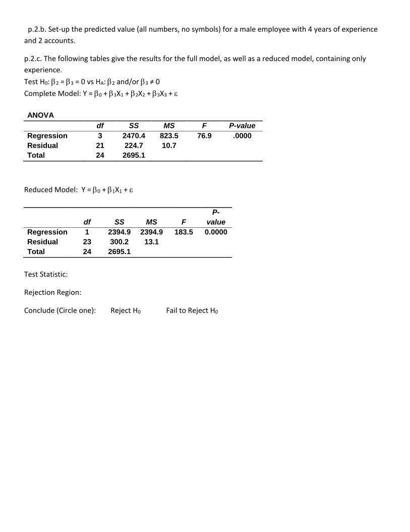
p.2.c. The following tables give the results for the full model, as well as a reduced model, containing only

experience.

Test H0: 2 = 3 = 0 vs HA: 2 and/or 3 ≠ 0

Complete Model: Y = 0 + 1X1 + 2X2 + 3X3 +

ANOVA

df SS MS F P-value

Regression 3 2470.4 823.5 76.9 .0000

Residual 21 224.7 10.7

Total 24 2695.1

Reduced Model: Y = 0 + 1X1 +

df SS MS F

P-

value

Regression 1 2394.9 2394.9 183.5 0.0000

Residual 23 300.2 13.1

Total 24 2695.1

Test Statistic:

Rejection Region:

Conclude (Circle one): Reject H0 Fail to Reject H0

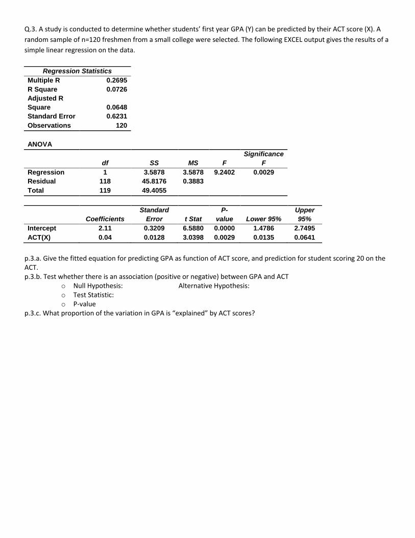
Q.3. A study is conducted to determine whether students’ first year GPA (Y) can be predicted by their ACT score (X). A

random sample of n=120 freshmen from a small college were selected. The following EXCEL output gives the results of a

simple linear regression on the data.

Regression Statistics

Multiple R 0.2695

R Square 0.0726

Adjusted R

Square 0.0648

Standard Error 0.6231

Observations 120

ANOVA

df SS MS F

Significance

F

Regression 1 3.5878 3.5878 9.2402 0.0029

Residual 118 45.8176 0.3883

Total 119 49.4055

Coefficients

Standard

Error t Stat

P-

value Lower 95%

Upper

95%

Intercept 2.11 0.3209 6.5880 0.0000 1.4786 2.7495

ACT(X) 0.04 0.0128 3.0398 0.0029 0.0135 0.0641

p.3.a. Give the fitted equation for predicting GPA as function of ACT score, and prediction for student scoring 20 on the ACT. p.3.b. Test whether there is an association (positive or negative) between GPA and ACT

o Null Hypothesis: Alternative Hypothesis: o Test Statistic: o P-value

p.3.c. What proportion of the variation in GPA is “explained” by ACT scores?

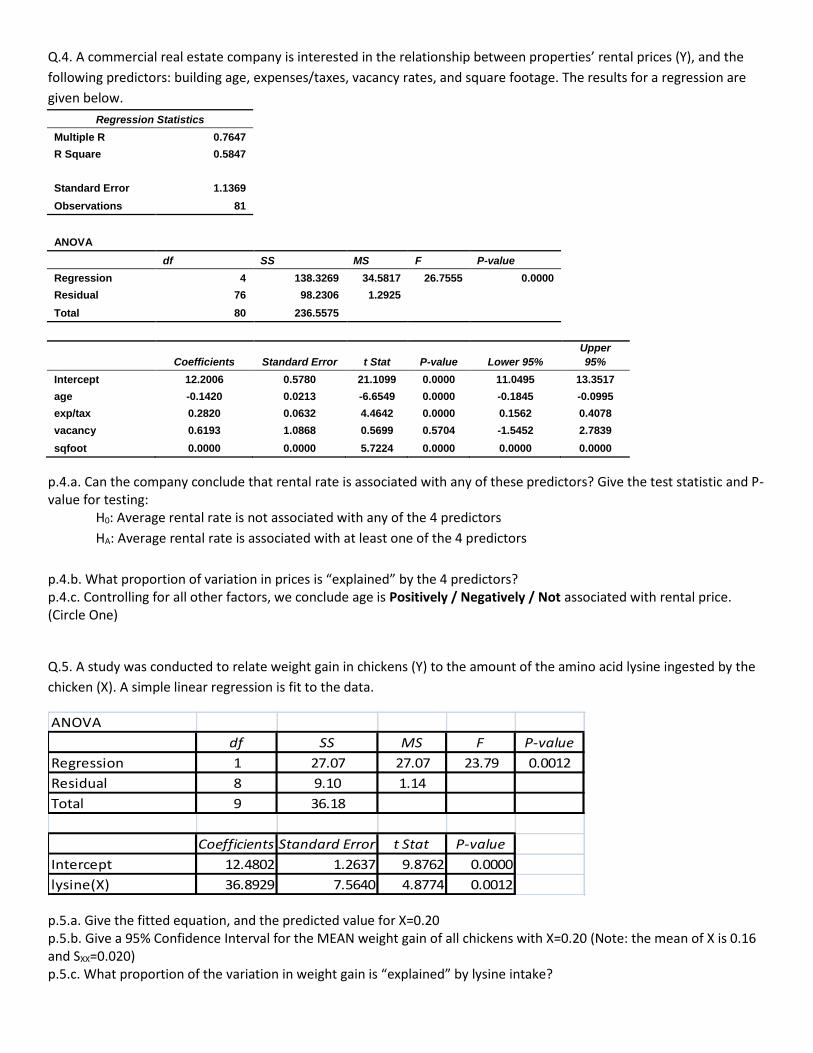
Q.4. A commercial real estate company is interested in the relationship between properties’ rental prices (Y), and the

following predictors: building age, expenses/taxes, vacancy rates, and square footage. The results for a regression are

given below.


Multiple R 0.7647

R Square 0.5847

Standard Error 1.1369

Observations 81

ANOVA

df SS MS F P-value

Regression 4 138.3269 34.5817 26.7555 0.0000

Residual 76 98.2306 1.2925

Total 80 236.5575

Coefficients Standard Error t Stat P-value Lower 95%

Upper

95%

Intercept 12.2006 0.5780 21.1099 0.0000 11.0495 13.3517

age -0.1420 0.0213 -6.6549 0.0000 -0.1845 -0.0995

exp/tax 0.2820 0.0632 4.4642 0.0000 0.1562 0.4078

vacancy 0.6193 1.0868 0.5699 0.5704 -1.5452 2.7839

sqfoot 0.0000 0.0000 5.7224 0.0000 0.0000 0.0000

p.4.a. Can the company conclude that rental rate is associated with any of these predictors? Give the test statistic and P-value for testing:

H0: Average rental rate is not associated with any of the 4 predictors

HA: Average rental rate is associated with at least one of the 4 predictors

p.4.b. What proportion of variation in prices is “explained” by the 4 predictors? p.4.c. Controlling for all other factors, we conclude age is Positively / Negatively / Not associated with rental price. (Circle One)

Q.5. A study was conducted to relate weight gain in chickens (Y) to the amount of the amino acid lysine ingested by the

chicken (X). A simple linear regression is fit to the data.

ANOVA

df SS MS F P-value

Regression 1 27.07 27.07 23.79 0.0012

Residual 8 9.10 1.14

Total 9 36.18

Coefficients Standard Error t Stat P-value

Intercept 12.4802 1.2637 9.8762 0.0000

lysine(X) 36.8929 7.5640 4.8774 0.0012

p.5.a. Give the fitted equation, and the predicted value for X=0.20 p.5.b. Give a 95% Confidence Interval for the MEAN weight gain of all chickens with X=0.20 (Note: the mean of X is 0.16 and SXX=0.020) p.5.c. What proportion of the variation in weight gain is “explained” by lysine intake?

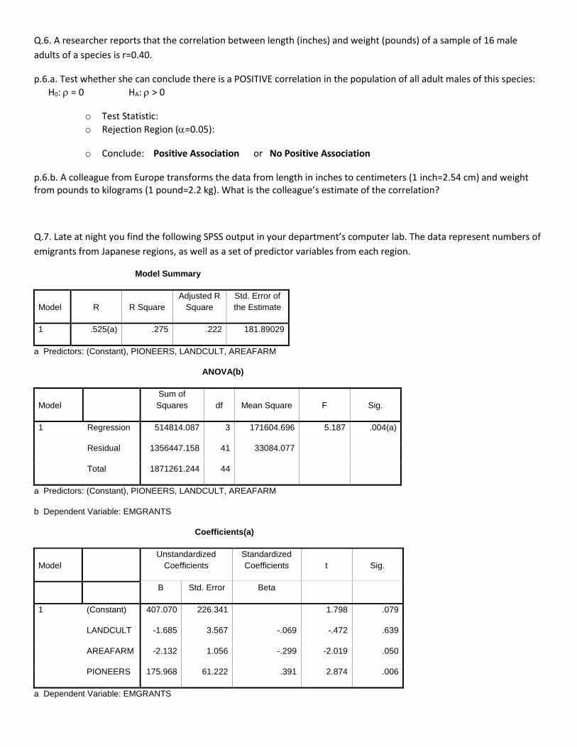
Q.6. A researcher reports that the correlation between length (inches) and weight (pounds) of a sample of 16 male

adults of a species is r=0.40.

p.6.a. Test whether she can conclude there is a POSITIVE correlation in the population of all adult males of this species:

H0: = 0 HA: > 0

o Test Statistic:

o Rejection Region (=0.05):

o Conclude: Positive Association or No Positive Association

p.6.b. A colleague from Europe transforms the data from length in inches to centimeters (1 inch=2.54 cm) and weight from pounds to kilograms (1 pound=2.2 kg). What is the colleague’s estimate of the correlation?

Q.7. Late at night you find the following SPSS output in your department’s computer lab. The data represent numbers of

emigrants from Japanese regions, as well as a set of predictor variables from each region.

Model Summary

Model R R Square

Adjusted R

Square

Std. Error of

the Estimate

1 .525(a) .275 .222 181.89029

a Predictors: (Constant), PIONEERS, LANDCULT, AREAFARM

ANOVA(b)

Model

Sum of

Squares df Mean Square F Sig.

1 Regression 514814.087 3 171604.696 5.187 .004(a)

Residual 1356447.158 41 33084.077

Total 1871261.244 44

a Predictors: (Constant), PIONEERS, LANDCULT, AREAFARM

b Dependent Variable: EMGRANTS

Coefficients(a)

Model

Unstandardized

Coefficients

Standardized

Coefficients t Sig.

B Std. Error Beta

1 (Constant) 407.070 226.341 1.798 .079

LANDCULT -1.685 3.567 -.069 -.472 .639

AREAFARM -2.132 1.056 -.299 -2.019 .050

PIONEERS 175.968 61.222 .391 2.874 .006

a Dependent Variable: EMGRANTS

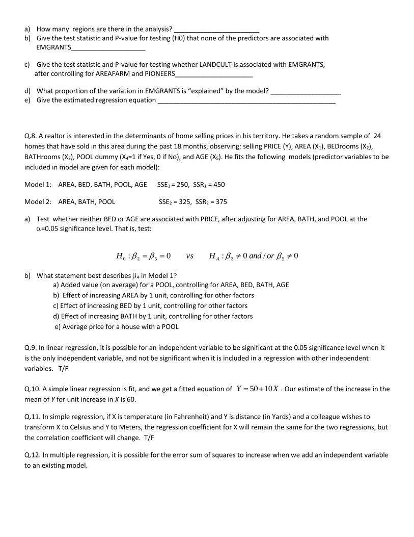
a) How many regions are there in the analysis? _______________________ b) Give the test statistic and P-value for testing (H0) that none of the predictors are associated with EMGRANTS____________________

c) Give the test statistic and P-value for testing whether LANDCULT is associated with EMGRANTS, after controlling for AREAFARM and PIONEERS_____________________

d) What proportion of the variation in EMGRANTS is “explained” by the model? ___________________ e) Give the estimated regression equation ________________________________________________

Q.8. A realtor is interested in the determinants of home selling prices in his territory. He takes a random sample of 24

homes that have sold in this area during the past 18 months, observing: selling PRICE (Y), AREA (X1), BEDrooms (X2),

BATHrooms (X3), POOL dummy (X4=1 if Yes, 0 if No), and AGE (X5). He fits the following models (predictor variables to be

included in model are given for each model):

Model 1: AREA, BED, BATH, POOL, AGE SSE1 = 250, SSR1 = 450

Model 2: AREA, BATH, POOL SSE2 = 325, SSR2 = 375

a) Test whether neither BED or AGE are associated with PRICE, after adjusting for AREA, BATH, and POOL at the

=0.05 significance level. That is, test:

0/0:0: 52520 orandHvsH A

b) What statement best describes 4 in Model 1? a) Added value (on average) for a POOL, controlling for AREA, BED, BATH, AGE

b) Effect of increasing AREA by 1 unit, controlling for other factors

c) Effect of increasing BED by 1 unit, controlling for other factors

d) Effect of increasing BATH by 1 unit, controlling for other factors

e) Average price for a house with a POOL

Q.9. In linear regression, it is possible for an independent variable to be significant at the 0.05 significance level when it

is the only independent variable, and not be significant when it is included in a regression with other independent

variables. T/F

Q.10. A simple linear regression is fit, and we get a fitted equation of 50 10Y X . Our estimate of the increase in the

mean of Y for unit increase in X is 60.

Q.11. In simple regression, if X is temperature (in Fahrenheit) and Y is distance (in Yards) and a colleague wishes to

transform X to Celsius and Y to Meters, the regression coefficient for X will remain the same for the two regressions, but

the correlation coefficient will change. T/F

Q.12. In multiple regression, it is possible for the error sum of squares to increase when we add an independent variable

to an existing model.

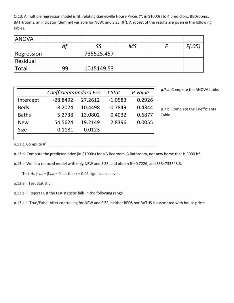
Q.13. A multiple regression model is fit, relating Gainesville House Prices (Y, in $1000s) to 4 predictors: BEDrooms,

BATHrooms, an indicator (dummy) variable for NEW, and SIZE (ft2). A subset of the results are given in the following

tables.

ANOVAdf SS MS F F(.05)

Regression 735525.457

Residual

Total 99 1015149.53

p.7.a. Complete the ANOVA table.

p.7.b. Complete the Coefficients

Table.

p.13.c. Compute R2 ____________________________________________________

p.13.d. Compute the predicted price (in $1000s) for a 3 Bedroom, 3 Bathroom, not new home that is 3000 ft2.

p.13.e. We fit a reduced model with only NEW and SIZE, and obtain R2=0.7226, and SSR=733543.3.

Test H0: Bed = Bath = 0 at the = 0.05 significance level:

p.13.e.i. Test Statistic:

p.13.e.ii. Reject H0 if the test statistic falls in the following range ________________________________

p.13.e.iii True/False: After controlling for NEW and SIZE, neither BEDS nor BATHS is associated with house prices.

CoefficientsStandard Error t Stat P-value

Intercept -28.8492 27.2612 -1.0583 0.2926

Beds -8.2024 10.4498 -0.7849 0.4344

Baths 5.2738 13.0802 0.4032 0.6877

New 54.5624 19.2149 2.8396 0.0055

Size 0.1181 0.0123

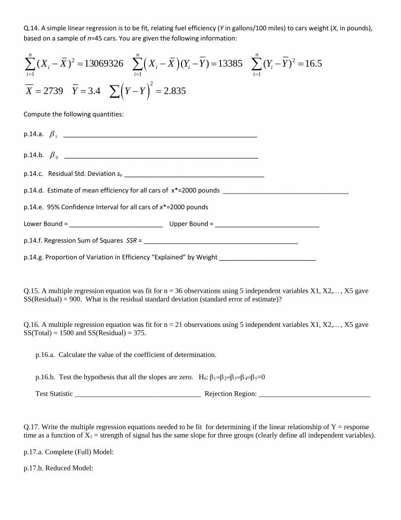
Q.14. A simple linear regression is to be fit, relating fuel efficiency (Y in gallons/100 miles) to cars weight (X, in pounds),

based on a sample of n=45 cars. You are given the following information:

2 2

1 1 1

2

( ) 13069326 ( ) 13385 ( ) 16.5

2739 3.4 2.835

n n n

i i i i

i i i

X X X X Y Y Y Y

X Y Y Y

Compute the following quantities:

p.14.a. 1 ______________________________________________________

p.14.b. 0 ______________________________________________________

p.14.c. Residual Std. Deviation se _______________________________________

p.14.d. Estimate of mean efficiency for all cars of x*=2000 pounds ___________________________________

p.14.e. 95% Confidence Interval for all cars of x*=2000 pounds

Lower Bound = __________________________ Upper Bound = _____________________________

p.14.f. Regression Sum of Squares SSR = ___________________________________________

p.14.g. Proportion of Variation in Efficiency “Explained” by Weight ___________________________

Q.15. A multiple regression equation was fit for n = 36 observations using 5 independent variables X1, X2,, X5 gave

SS(Residual) = 900. What is the residual standard deviation (standard error of estimate)?

Q.16. A multiple regression equation was fit for n = 21 observations using 5 independent variables X1, X2,, X5 gave

SS(Total) = 1500 and SS(Residual) = 375.

p.16.a. Calculate the value of the coefficient of determination.

p.16.b. Test the hypothesis that all the slopes are zero. H0: =0

Test Statistic ___________________________________ Rejection Region: _______________________________

Q.17. Write the multiple regression equations needed to be fit for determining if the linear relationship of Y = response

time as a function of X1 = strength of signal has the same slope for three groups (clearly define all independent variables).

p.17.a. Complete (Full) Model:

p.17.b. Reduced Model:

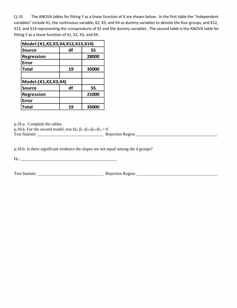
Q.18. The ANOVA tables for fitting Y as a linear function of X are shown below. In the first table the “independent

variables” include X1, the continuous variable, X2, X3, and X4 as dummy variables to denote the four groups, and X12,

X13, and X14 representing the crossproducts of X1 and the dummy variables. The second table is the ANOVA table for

fitting Y as a linear function of X1, X2, X3, and X4.

Model:(X1,X2,X3,X4,X12,X13,X14)

Source df SS

Regression 28000

Error

Total 19 35000

Model:(X1,X2,X3,X4)

Source df SS

Regression 21000

Error

Total 19 35000

p.18.a. Complete the tables.

p.18.b. For the second model, test H0 = 0

Test Statistic _______________________________ Rejection Region ______________________________________

p.18.b. Is there significant evidence the slopes are not equal among the 4 groups?

H0: _____________________________________________


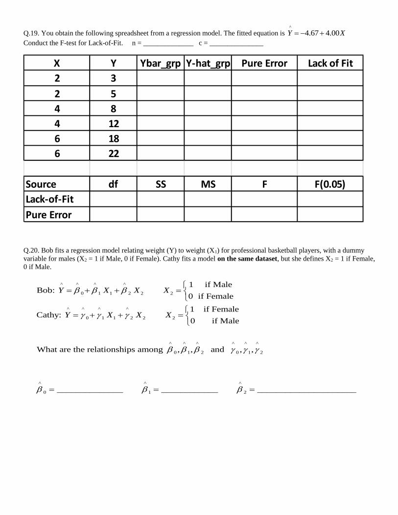
Q.19. You obtain the following spreadsheet from a regression model. The fitted equation is ^

4.67 4.00Y X

Conduct the F-test for Lack-of-Fit. n = ______________ c = _______________

X Y Ybar_grp Y-hat_grp Pure Error Lack of Fit

2 3

2 5

4 8

4 12

6 18

6 22

Source df SS MS F F(0.05)

Lack-of-Fit

Pure Error

Q.20. Bob fits a regression model relating weight (Y) to weight (X1) for professional basketball players, with a dummy

variable for males (X2 = 1 if Male, 0 if Female). Cathy fits a model on the same dataset, but she defines X2 = 1 if Female,

0 if Male.

^ ^ ^ ^

0 1 21 2 2

^ ^ ^ ^

0 1 21 2 2

^ ^ ^ ^ ^ ^

0 1 2 0 1 2

^ ^

0 1

1 if MaleBob:

0 if Female

1 if FemaleCathy:

0 if Male

What are the relationships among , , and , ,

______________ __

Y X X X

Y X X X

^

2__________ _____________________

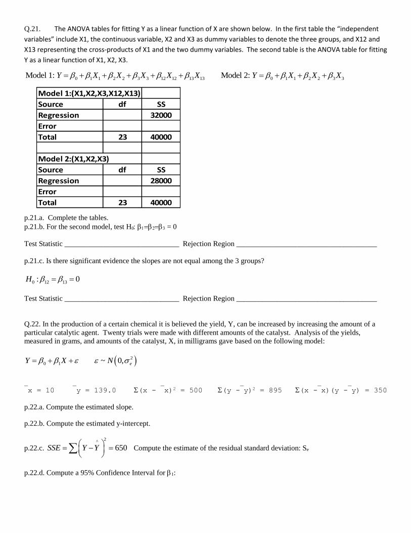
Q.21. The ANOVA tables for fitting Y as a linear function of X are shown below. In the first table the “independent

variables” include X1, the continuous variable, X2 and X3 as dummy variables to denote the three groups, and X12 and

X13 representing the cross-products of X1 and the two dummy variables. The second table is the ANOVA table for fitting

Y as a linear function of X1, X2, X3.

0 1 1 2 2 3 3 12 12 13 13 0 1 1 2 2 3 3Model 1: Model 2: Y X X X X X Y X X X

Model 1:(X1,X2,X3,X12,X13)

Source df SS

Regression 32000

Error

Total 23 40000

Model 2:(X1,X2,X3)

Source df SS

Regression 28000

Error

Total 23 40000


p.21.b. For the second model, test H0 = 0


p.21.c. Is there significant evidence the slopes are not equal among the 3 groups?

0 12 13: 0H


Q.22. In the production of a certain chemical it is believed the yield, Y, can be increased by increasing the amount of a

particular catalytic agent. Twenty trials were made with different amounts of the catalyst. Analysis of the yields,

measured in grams, and amounts of the catalyst, X, in milligrams gave based on the following model:

2

0 1 ~ 0, eY X N

x = 10 y = 139.0 (x - x)2 = 500 (y -y)2 = 895 (x -x)(y -y) = 350

p.22.a. Compute the estimated slope.

p.22.b. Compute the estimated y-intercept.

p.22.c.

2^

650SSE Y Y

Compute the estimate of the residual standard deviation: Se

p.22.d. Compute a 95% Confidence Interval for 1:

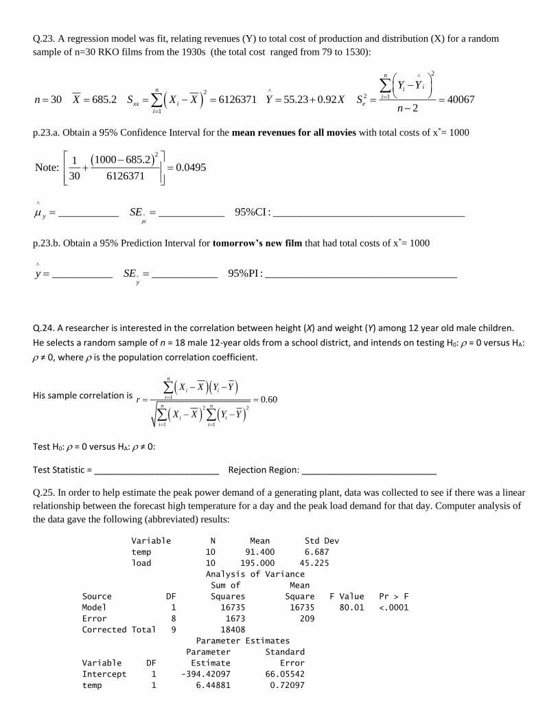
Q.23. A regression model was fit, relating revenues (Y) to total cost of production and distribution (X) for a random

sample of n=30 RKO films from the 1930s (the total cost ranged from 79 to 1530):

2^

^22 1

1

30 685.2 6126371 55.23 0.92 400672

n

iini

xx i e

i

Y Y

n X S X X Y X Sn

p.23.a. Obtain a 95% Confidence Interval for the mean revenues for all movies with total costs of x*= 1000

2

1000 685.21Note: 0.0495

30 6126371

^

^

___________ ____________ 95%CI : ___________________________________y SE

p.23.b. Obtain a 95% Prediction Interval for tomorrow’s new film that had total costs of x*= 1000

^

^

___________ ____________ 95%PI : ___________________________________y

y SE

Q.24. A researcher is interested in the correlation between height (X) and weight (Y) among 12 year old male children.

He selects a random sample of n = 18 male 12-year olds from a school district, and intends on testing H0: = 0 versus HA:

≠ 0, where is the population correlation coefficient.

His sample correlation is

1

2 2

1 1

0.60

n

i i

i

n n

i i

i i

X X Y Y

r

X X Y Y

Test H0: = 0 versus HA: ≠ 0:

Test Statistic = _________________________ Rejection Region: ___________________________

Q.25. In order to help estimate the peak power demand of a generating plant, data was collected to see if there was a linear

relationship between the forecast high temperature for a day and the peak load demand for that day. Computer analysis of

the data gave the following (abbreviated) results:

Variable N Mean Std Dev

temp 10 91.400 6.687

load 10 195.000 45.225

Analysis of Variance

Sum of Mean

Source DF Squares Square F Value Pr > F

Model 1 16735 16735 80.01 <.0001

Error 8 1673 209

Corrected Total 9 18408

Parameter Estimates

Parameter Standard

Variable DF Estimate Error

Intercept 1 -394.42097 66.05542

temp 1 6.44881 0.72097

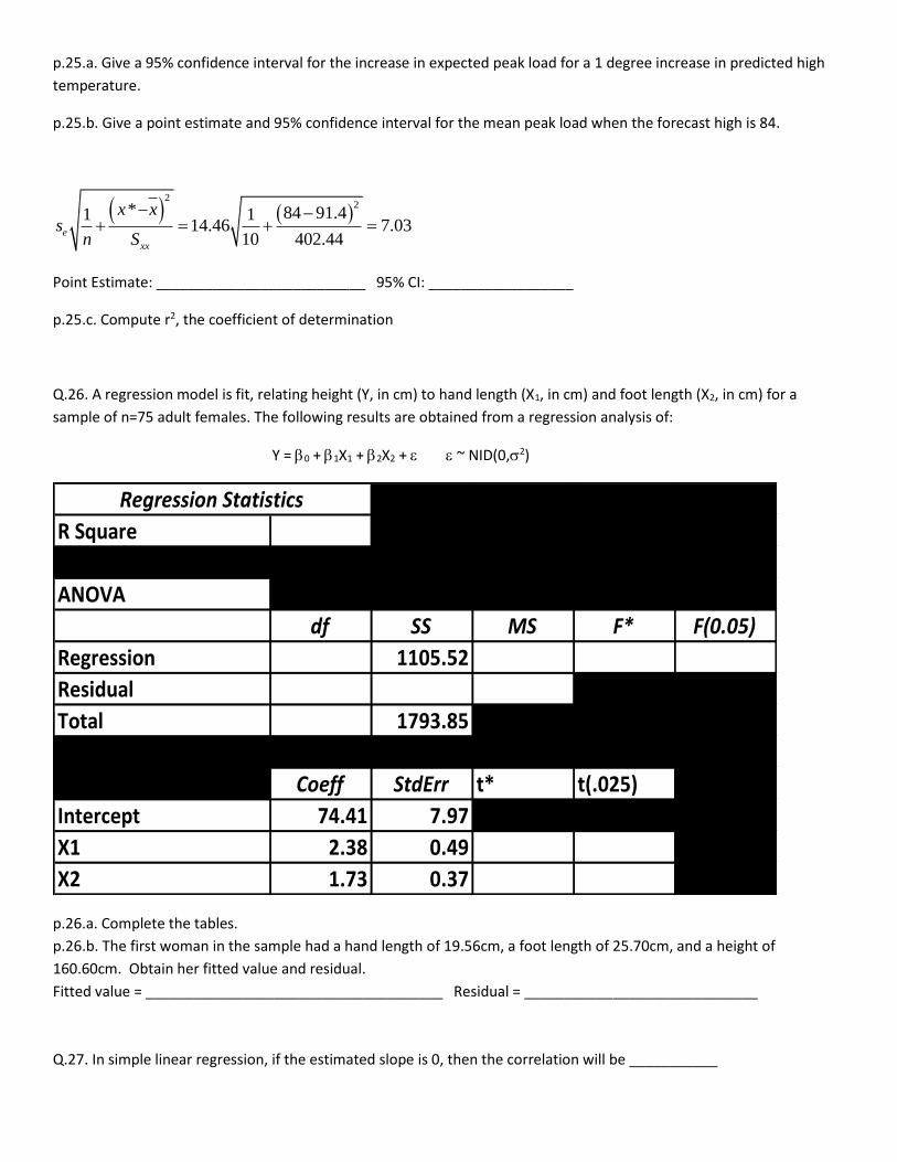
p.25.a. Give a 95% confidence interval for the increase in expected peak load for a 1 degree increase in predicted high

temperature.

p.25.b. Give a point estimate and 95% confidence interval for the mean peak load when the forecast high is 84.

2

2* 84 91.41 114.46 7.03

10 402.44e

xx

x xs

n S

Point Estimate: __________________________ 95% CI: __________________

p.25.c. Compute r2, the coefficient of determination

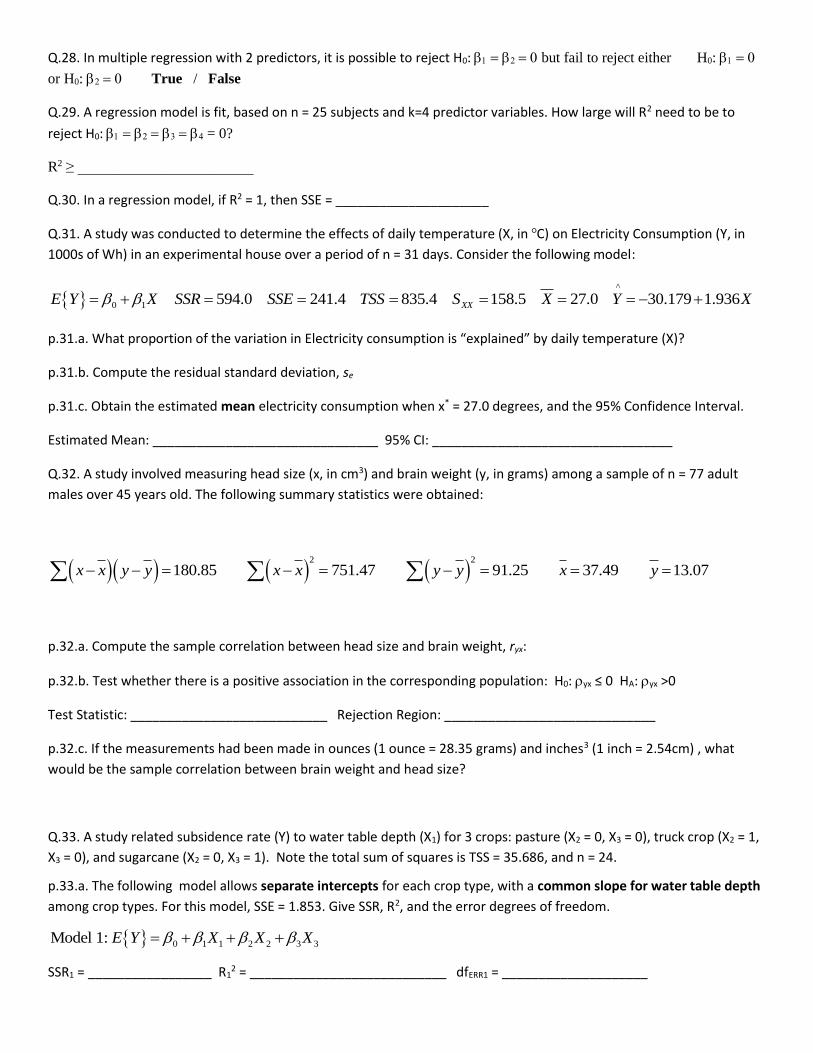
Q.26. A regression model is fit, relating height (Y, in cm) to hand length (X1, in cm) and foot length (X2, in cm) for a

sample of n=75 adult females. The following results are obtained from a regression analysis of:

Y = 0 + 1X1 + 2X2 + ~ NID(0,2)


R Square

ANOVA

df SS MS F* F(0.05)

Regression 1105.52

Residual #N/A

Total 1793.85 #N/A #N/A #N/A

Coeff StdErr t* t(.025)

Intercept 74.41 7.97 #N/A #N/A #N/A

X1 2.38 0.49 #N/A

X2 1.73 0.37 #N/A


p.26.b. The first woman in the sample had a hand length of 19.56cm, a foot length of 25.70cm, and a height of

160.60cm. Obtain her fitted value and residual.

Fitted value = _____________________________________ Residual = _____________________________

Q.27. In simple linear regression, if the estimated slope is 0, then the correlation will be ___________

Q.28. In multiple regression with 2 predictors, it is possible to reject H0: but fail to reject either H0:

or H0: True / False

Q.29. A regression model is fit, based on n = 25 subjects and k=4 predictor variables. How large will R2 need to be to

reject H0: = 0?

R2 ≥ ________________________

Q.30. In a regression model, if R2 = 1, then SSE = _____________________

Q.31. A study was conducted to determine the effects of daily temperature (X, in ○C) on Electricity Consumption (Y, in

1000s of Wh) in an experimental house over a period of n = 31 days. Consider the following model:

^

0 1 594.0 241.4 835.4 158.5 27.0 30.179 1.936XXE Y X SSR SSE TSS S X Y X

p.31.a. What proportion of the variation in Electricity consumption is “explained” by daily temperature (X)?

p.31.b. Compute the residual standard deviation, se

p.31.c. Obtain the estimated mean electricity consumption when x* = 27.0 degrees, and the 95% Confidence Interval.

Estimated Mean: _______________________________ 95% CI: _________________________________

Q.32. A study involved measuring head size (x, in cm3) and brain weight (y, in grams) among a sample of n = 77 adult

males over 45 years old. The following summary statistics were obtained:

2 2

180.85 751.47 91.25 37.49 13.07x x y y x x y y x y

p.32.a. Compute the sample correlation between head size and brain weight, ryx:

p.32.b. Test whether there is a positive association in the corresponding population: H0: yx ≤ 0 HA: yx >0

Test Statistic: ___________________________ Rejection Region: _____________________________

p.32.c. If the measurements had been made in ounces (1 ounce = 28.35 grams) and inches3 (1 inch = 2.54cm) , what

would be the sample correlation between brain weight and head size?

Q.33. A study related subsidence rate (Y) to water table depth (X1) for 3 crops: pasture (X2 = 0, X3 = 0), truck crop (X2 = 1,

X3 = 0), and sugarcane (X2 = 0, X3 = 1). Note the total sum of squares is TSS = 35.686, and n = 24.

p.33.a. The following model allows separate intercepts for each crop type, with a common slope for water table depth

among crop types. For this model, SSE = 1.853. Give SSR, R2, and the error degrees of freedom.

0 1 1 2 2 3 3Model 1: E Y X X X

SSR1 = _________________ R12 = ___________________________ dfERR1 = ____________________

p.33.b. The following model allows separate intercepts for each crop types, with separate slopes for water table depth


0 1 1 2 2 3 3 12 1 2 13 1 3Model 2: E Y X X X X X X X

SSR2 = _________________ R22 = ___________________________ dfERR2 = ____________________

p.33.c. Test whether the slopes are the same for the 3 crop types. H0: 12 = 13 = 0

Test Statistic: ____________________________ Rejection Region: ___________________________

Q.34. In simple linear regression, if the estimated slope is 0, then the correlation will be ___________

Q.35. In multiple regression with 2 predictors, it is possible to reject H0: but fail to reject either H0:

or H0: True / False

Q.36. A regression model is fit, based on n = 25 subjects and k=4 predictor variables. How large will R2 need to be to

reject H0: = 0?

R2 ≥ ________________________

Q.37. In a regression model, if R2 = 1, then SSE = _____________________

Q.38. A study was conducted to determine the effects of daily temperature (X, in ○C) on Electricity Consumption (Y, in

1000s of Wh) in an experimental house over a period of n = 31 days. Consider the following model:

^

0 1 594.0 241.4 835.4 158.5 27.0 30.179 1.936XXE Y X SSR SSE TSS S X Y X

p.38.a. What proportion of the variation in Electricity consumption is “explained” by daily temperature (X)?

p.38.b. Compute the residual standard deviation, se

p.38.c. Obtain the estimated mean electricity consumption when x* = 27.0 degrees, and the 95% Confidence Interval.

Estimated Mean: _______________________________ 95% CI: _________________________________

Q.39. A study involved measuring head size (x, in cm3) and brain weight (y, in grams) among a sample of n = 77 adult

males over 45 years old. The following summary statistics were obtained:

2 2

180.85 751.47 91.25 37.49 13.07x x y y x x y y x y

p.39.a. Compute the sample correlation between head size and brain weight, ryx:

p.39.b. Test whether there is a positive association in the corresponding population: H0: yx ≤ 0 HA: yx >0

Test Statistic: ___________________________ Rejection Region: _____________________________

p.39.c. If the measurements had been made in ounces (1 ounce = 28.35 grams) and inches3 (1 inch = 2.54cm) , what

would be the sample correlation between brain weight and head size?

Q.40. A study related subsidence rate (Y) to water table depth (X1) for 3 crops: pasture (X2 = 0, X3 = 0), truck crop (X2 = 1,

X3 = 0), and sugarcane (X2 = 0, X3 = 1). Note the total sum of squares is TSS = 35.686, and n = 24.

p.40.a. The following model allows separate intercepts for each crop type, with a common slope for water table depth


0 1 1 2 2 3 3Model 1: E Y X X X

SSR1 = _________________ R12 = ___________________________ dfERR1 = ____________________

p.40.b. The following model allows separate intercepts for each crop types, with separate slopes for water table depth


0 1 1 2 2 3 3 12 1 2 13 1 3Model 2: E Y X X X X X X X

SSR2 = _________________ R22 = ___________________________ dfERR2 = ____________________

p.40.c. Test whether the slopes are the same for the 3 crop types. H0: 12 = 13 = 0

Test Statistic: ____________________________ Rejection Region: ___________________________

linear regression problems - department of statisticswinner/sta6166/linear_regression.pdf ·...

Documents