linear quadratic gaussian (lqg) c ontroller design...

LINEAR QUADRATIC GAUSSIAN (LQG) CONTROLLER DESIGN FOR

SERVO MOTOR

WAN SYAHIDAH BINTI WAN MOHD

A project report submitted in partialfulfillment of the requirementsfor the award of the

Degree of Master of Electrical Engineering

Faculty of Electrical and Electronic EngineeringUniversity Tun Hussein Onn Malaysia

JUNE 2013

v

ABSTRACT

This paper presents the development of Linear Quadratic Gaussian controller design

forDC servo motor.The accuracy of the control system is directly proportional to

servo motor precision. However, the precision of DC servo motor system difficult to

achieved due to the ignorance of the sensor noise and plant disturbance. Therefore

LQG controller has been design to control speed and position of DC servo motor. In

LQG controller designed, the noise sensor and plant disturbance has been considered

as white noise Gaussian. This controller has be designed based on combination of

Steady-state Linear Quadratic (LQ)OptimalControl and Steady-state Kalman Filter

State Estimation by solving matrix Riccati equation in order to determine steady-

state feedback gain, K and steady-state Kalman gain, G. MATLAB Simulink and M-

File approached have been done to simulate the design. Besides that, Arduino

microcontroller board also has been explored in order to do real-time Simulation

between LQG controller and DC servo motor. The step response of closed-loop

digital control system using LQG controller and opened-loop control system have

been compared to verified that the performance of closed-loop control system better

than opened-loop system

vi

ABSTRAK

Kertas kerja ini membentangkan perkembangan rekabentuk pengawal Linear

Kuadratik Gaussian (LQG) bagi motor servo arus terus. Ketepatan system kawalan

adalah berkadar langsung dengan ketepatan motor servo. Walaubagaimanapun,

ketepatan servo motor arus terus sukar untuk dicapai disebabkan oleh pengabaian

bunyi sensor dan gangguan sistem. Oleh sebab itu, pengawal LQG telah dicipta

untuk mengawal kelajuan dan kedudukan motor servo arus terus. Dalam perekaan

pengawal LQG, bunyi sensor dan gangguan system telah dianggap sebagai putih

hingar Gaussian. Pengawal ini telah dibina berdasarkan gabungan keadaan mantap

Linear Kuadratic (LQ) Kawalan Optimum dan keadaan mantap anggaran penapis

Kalman dengan menyelesaikan persamaan matrik Riccati bagi menentukan gandaan

maklumbalas keadaan mantap, K dan gandaan Kalman keadaan mantap, G.

Pendekatan menggunakan perisian MATLAB Simulink dan M-Fail telah dilakukan

bagi mensimulasikan rekabentuk pengawal. Selain itu, papan Arduino

mikropengawal juga telah dikaji untuk melakukan simulasi masa nyataa ntara

pengawal LQG dan motor servo arus terus. Sambutan langkah gelung tertutup

system kawalan digital menggunakan pengawal LQG dan system kawalan gelung

terbuka telah dibandingkan untuk mengesahkan bahawa prestasi system kawalan

gelung tertutup adalah lebih baik berbanding system gelung terbuka.

vii

TABLE OF CONTENTS

TITLE i

DECLARATION ii

DEDICATION iii

ACKNOWLEDGEMENT iv

ABSTRACT v

ABSTRAK vi

TABLE OF CONTENTS vii

LIST OF TABLES xii

LIST OF FIGURE xiii

LIST OF SYMBOLS AND ABBREVIATION xvi

LIST OF APPENDICES xviii

CHAPTER 1 INTRODUCTION 1

1.1 Project Background 1

1.2 Problem Statement 2

1.3 Objectives of Project 2

1.4 Scope of project 2

1.5 Thesis Outline 3

CHAPTER 2 LITERATURE REVIEW 4

2.1 Introduction 4

2.2 Transient Response Specification of Control 5

System

2.3 DC Servo motor Modelling 6

viii

2.4 Controllability and Observability 8

2.5 Optimal Control 9

2.6 The Quadratic Cost Function 10

2.7 The Principle of Optimality 11

2.8 Linear Quadratic Optimal Control 12

2.9 Steady-State Quadratic Optimal Control 13

2.10 State Estimation 15

2.10.1 Observer Model 15

2.10.2 Errors in Estimation 17

2.11 Optimal State Estimation – Kalman Filters 18

2.11.1 The Discrete Kalman Filter Algorithm 21

2.12 Linear Quadratic Gaussian (LQG) 22

2.13 Matrix Laboratory (MATLAB) 23

2.14 Arduino Mega 2560 23

2.15 Motor Driver L293D 24

2.16 Motor ID23005 25

2.17 Optical Encoder 26

2.18 Overview of Previous Project 27

2.18.1 Case Study 1 27





2.18.6 Comparison of Case Study 30

2.19 Conclusions 31

CHAPTER 3 METHODOLOGY 32

3.1 Introduction 32

3.2 The Development of Flow Chart 33

3.3 Mathematical Model of Servo Motor 35

3.3.1 Parameter of DC Servo Motor 35

3.3.2 Continuous Transfer Function of DC 35

Servo Motor

3.3.3 Continuous State Space for DC Servo 37

ix

Motor

3.3.3.1 Third Order DC Servo Motor 38

3.3.3.2 Second Order DC Servo Motor

403.3.4 Implementation of DC Servo

Motor 42

into MATLAB


3.3.4.2 Second Order DC Servo Motor 43

3.4 Linear Quadratic (LQ) Optimal Control 43

3.5 Kalman Filter Optimal State Estimation 47

3.6 Linear Quadratic Gaussian (LQG) of DC 49

Servo Motor

3.7 Control DC Servo Motor 55

3.3.1 Control Motor using Direct Current 55

(DC) supply

3.3.2 Control Motor using Motor Driver 55

IC L293D


3.9 DC Servo Motor and Optical Encoder 58

3.10 Conclusion 59

CHAPTER 4 RESULT AND DISCUSSIONS 61

4.1 Introduction 61

4.2 Mathematical Model of Servo Motor 61

4.2.1 Continuous State Space for DC Servo 61

Motor



4.2.2 Continuous Transfer Function of DC 64

Servo Motor



4.2.3 Discrete State Space for DC Servo Motor 65

x



4.2.4 Discrete Transfer Function of DC Servo 67

Motor



4.2.5 Analysis of Open-loop DC Servo Motor 68

System



4.3 Controllability and Observability 72

4.3.1 Third Order DC Servo Motor 72

4.3.2 Second Order DC Servo Motor 73

4.4 Linear Quadratic (LQ) Optimal Control 74



4.5 Kalman Filter Optimal State Estimation 75



4.6 Linear Quadratic Gaussian (LQG) Controller 77



4.7 Digital Control System 79

4.7.1 Digital Control System to Control Position 79

4.7.2 Digital Control System to Control Speed 79

4.8 Analysis of Digital Control System 80

4.8.1 Digital Control System to Control Position 80

4.8.2 Digital Control System to Control Speed 82

4.9 Comparison of Open-loop and Closed-loop System 83

4.9.1 Control System to Control Position 83

4.9.2 Control System to Control Speed 84

4.10 Control DC Servo Motor 85

4.10.1 Control Motor using Direct Current 85

(DC) supply

xi

4.10.2 Control Motor using Motor Driver IC 86

L293D

4.11 Optical Encoder Count 87

4.12 DC Servo Motor and Optical Encoder 88

4.13 Conclusion 90

CHAPTER 5 CONCLUSION AND RECOMMENDATIONS 92

5.1 Conclusion 92

5.2 Recommendations for Future Works 92

REFERENCES 94

APPENDICES 97

VITA 112

xii

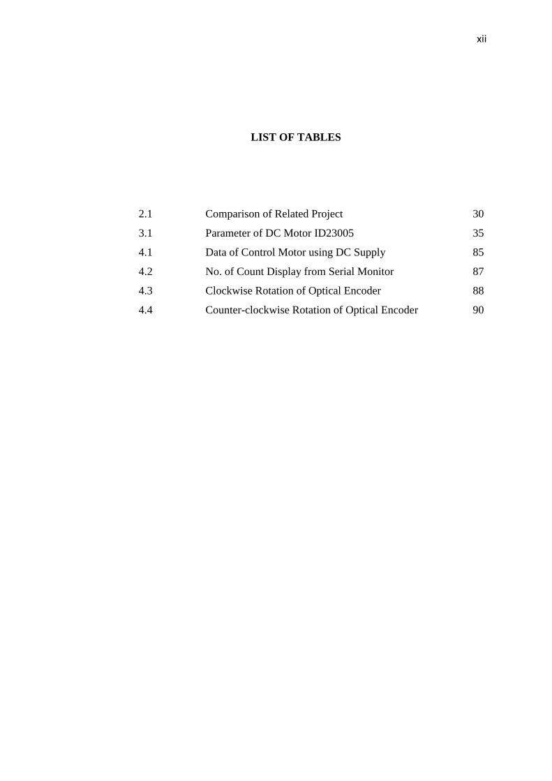
LIST OF TABLES

2.1 Comparison of Related Project 30

3.1 Parameter of DC Motor ID23005 35

4.1 Data of Control Motor using DC Supply 85

4.2 No. of Count Display from Serial Monitor 87

4.3 Clockwise Rotation of Optical Encoder 88

4.4 Counter-clockwise Rotation of Optical Encoder 90

xiii

LIST OF FIGURES

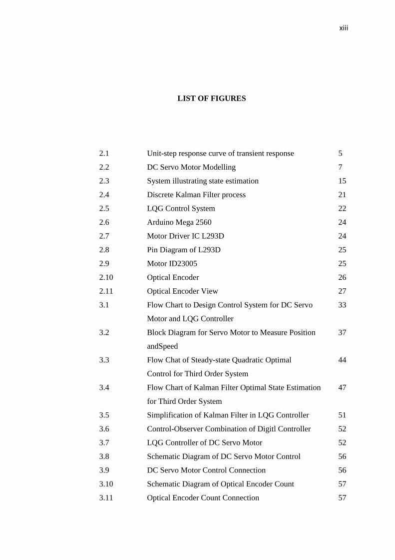
2.1 Unit-step response curve of transient response 5

2.2 DC Servo Motor Modelling 7

2.3 System illustrating state estimation 15

2.4 Discrete Kalman Filter process 21

2.5 LQG Control System 22

2.6 Arduino Mega 2560 24

2.7 Motor Driver IC L293D 24

2.8 Pin Diagram of L293D 25

2.9 Motor ID23005 25


2.11 Optical Encoder View 27

3.1 Flow Chart to Design Control System for DC Servo 33

Motor and LQG Controller

3.2 Block Diagram for Servo Motor to Measure Position 37

andSpeed

3.3 Flow Chat of Steady-state Quadratic Optimal 44

Control for Third Order System

3.4 Flow Chart of Kalman Filter Optimal State Estimation 47

for Third Order System

3.5 Simplification of Kalman Filter in LQG Controller 51

3.6 Control-Observer Combination of Digitl Controller 52

3.7 LQG Controller of DC Servo Motor 52

3.8 Schematic Diagram of DC Servo Motor Control 56

3.9 DC Servo Motor Control Connection 56

3.10 Schematic Diagram of Optical Encoder Count 57

3.11 Optical Encoder Count Connection 57

xiv

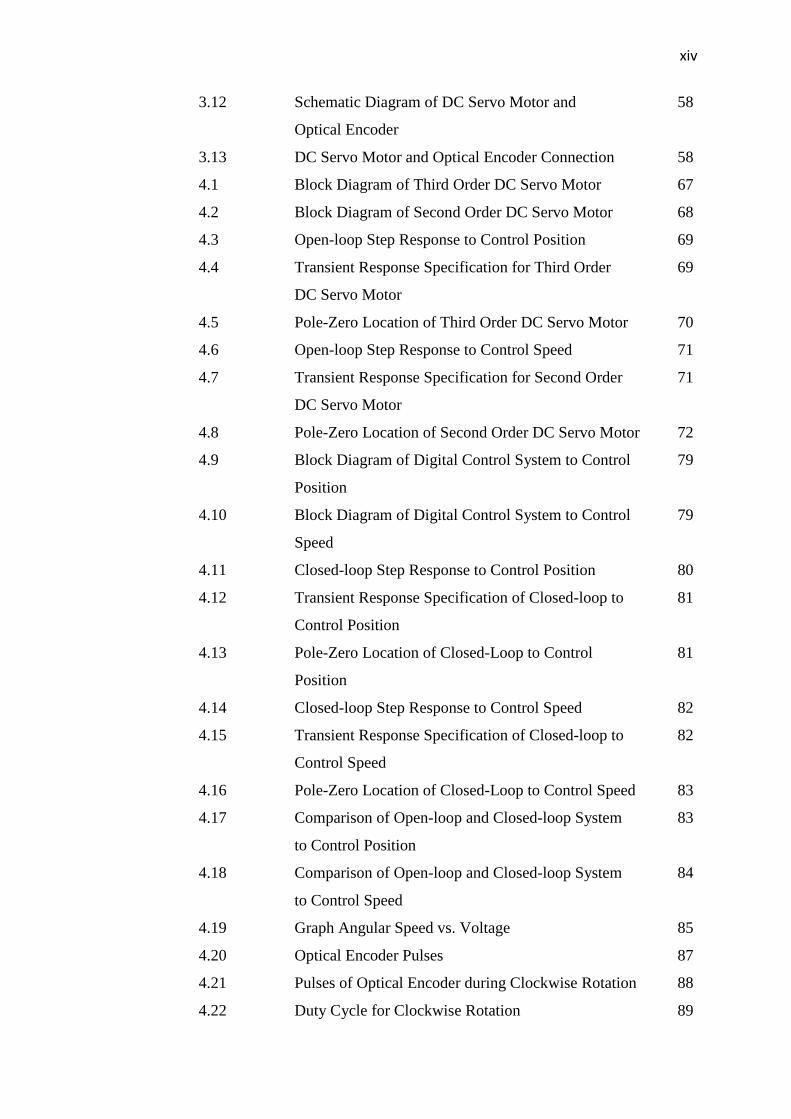
3.12 Schematic Diagram of DC Servo Motor and 58

Optical Encoder

3.13 DC Servo Motor and Optical Encoder Connection 58

4.1 Block Diagram of Third Order DC Servo Motor 67

4.2 Block Diagram of Second Order DC Servo Motor 68

4.3 Open-loop Step Response to Control Position 69

4.4 Transient Response Specification for Third Order 69

DC Servo Motor

4.5 Pole-Zero Location of Third Order DC Servo Motor 70

4.6 Open-loop Step Response to Control Speed 71

4.7 Transient Response Specification for Second Order 71

DC Servo Motor

4.8 Pole-Zero Location of Second Order DC Servo Motor 72

4.9 Block Diagram of Digital Control System to Control 79

Position

4.10 Block Diagram of Digital Control System to Control 79

Speed

4.11 Closed-loop Step Response to Control Position 80

4.12 Transient Response Specification of Closed-loop to 81

Control Position

4.13 Pole-Zero Location of Closed-Loop to Control 81

Position

4.14 Closed-loop Step Response to Control Speed 82

4.15 Transient Response Specification of Closed-loop to 82

Control Speed

4.16 Pole-Zero Location of Closed-Loop to Control Speed 83


to Control Position


to Control Speed

4.19 Graph Angular Speed vs. Voltage 85

4.20 Optical Encoder Pulses 87

4.21 Pulses of Optical Encoder during Clockwise Rotation 88

4.22 Duty Cycle for Clockwise Rotation 89

xv

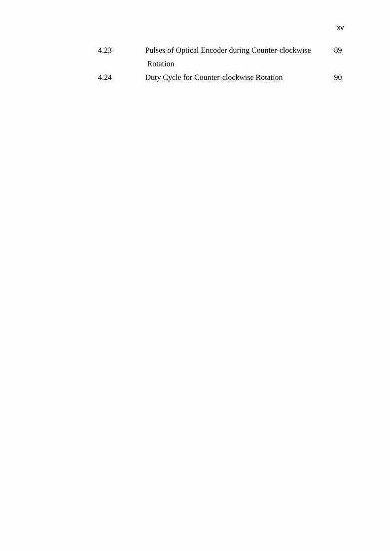
4.23 Pulses of Optical Encoder during Counter-clockwise 89

Rotation

4.24 Duty Cycle for Counter-clockwise Rotation 90

xvi

LIST OF SYMBOLS AND ABBREVIATION

LQG - Linear Quadratic Gaussian

LQR - Linear quadratic Regulator

LQ - Linear Quadratic

MATLAB - Matrix Laboratory

GUI - Graphical Interface User

LEQ - Linear Estimation Quadratic

LTR - Loop Transfer Recovery

EMF - Electromotive Force

DARE - Discrete Algebraic Riccati Equation

DC - Direct Current

BDC - Brush Direct Current

IR LED - Infrared Light emitting diode

GA - Genetic Algorithm

IC - Integrated Circuit

PWM - Pulse Width Modulation

td - Delay Time

tr - Rise Time

tp - Peak Time

Mp - Maximum Overshoot

ts - Settling Time

Ra - Armature Resistance

La - Armature Inductance

Va - Armature Voltage

ia - Armature Current

Tm - Torque

eb - Back Electromotive Force (Back EMF)

xvii

Jm - Motor Inertia

Bm - Viscous Damping Coefficient

ωm - Angular Velocity

θm - Angular Displacement

α - Angular Acceleration

Kb - Back-EMF Constant

Kt - Torque Constant

JG - Mass moment inertia

JL - Momenr of inertia of the load

JN - Performance Index

σ2 - Variance

Ke - Voltage Constant

Gs - Continuous Transfer Function

Gz - Discrete Transfer Function

P - Steady-state Riccati Equation

K - Optimal Feedback Gain Matrix

G - Steady-state Kalman Gain

- Duration of DC servo motor ON

T - Period of the rotation of DC servo motor in one cycle

xviii

LIST OF APPENDICES

A Gantt chart for Master Project 1 97

B Gantt chart for Master Project 2 98

C M-File Coding to Control Position of DC Servo Motor 99

D M-File Coding to Control Speed of DC Servo Motor 103

E Arduino Coding to Control DC Servo Motor 107

F Arduino Coding to Count Optical Encoder 109

G Arduino Coding for DC Servo Motor and Optical Encoder 110

CHAPTER 1

INTRODUCTION

1.1 Project Background

Servo motor is a motor that is used to control position or speed in closed-loop control

systems. It is generally designed for the computer, numeric control machines,

industrial equipment, weapon industry, speed control of alternators and to control

mechanism of full automatic regulators as the first starter, and also to quickly and

correctly starting a system. In the field of control mechanical linkages and robots,

research works are mostly found on DC motors. Therefore the requirement of a servo

motor is to turn over a wide range of speeds and also to perform position and speed

based on instruction given has been developed.

Properties of DC motor such like inertia, physical structure, shaft resonance

and shaft characteristics, electrical and physical constant are variable. Besides that,

the velocity and position tolerance of servo motor which are used at the control

systems are nearly identical. Therefore, servo motor must be controlled to ensure the

stability of the close-loop control system. Thus, Linear Quadratic Gaussian (LQG)

controller has been proposed to control the speed and position of servo motor.

Linear Quadratic Gaussian control is one of the most fundamental optimal

control problems that concerns uncertain linear systems disturbed by additive white

Gaussian noise. LQG controller is simply the combination of a Linear Quadratic

(LQ) Optimal Control and Kalman Filter State Estimation.

2

1.2 Problem Statement

Servo motors have received great attention in recent decades. Compare to other

motor types, servo motors can deliver more torque and power for the same size.

Besides that, it also provides safe and reliable operation and requires less

maintenance which make the used of servo motor received a great attention.

Specifically, with latest development in microprocessor and power electronics, very

accurate and highly efficient servo motor control systems have been developed. The

need for a feedback element was required in order to make control system

stable.However, the feedback not only increases the cost but also makes the control

of position and speed of servo motor becomes complex Further, the control accuracy

is directly proportional the precision of servo motor control. However, the precision

of servo motor control has been difficult to achieve due to the ignorance of the plant

disturbance and inaccuracies in feedback measurement cause by sensor noise.

Therefore, Linear Quadratic Gaussian (LQG)controller has been proposed to

overcome the sensor less position and speed control due to this problem.The main

proposed alternative of this project were to control and estimate the motor position

and speed besides to overcome the weakness of other digital controller.

1.3 Objectives of Project

The main objective of this project was to design and develop controller for servo

motor. Besides that, the goals that want to be achieves are:

i. To design Linear Quadratic Gaussian (LQG) controller for servo motor.

ii. To control the position and speed of servo motor with Linear Quadratic

Gaussian using MATLAB software.

iii. To analyse the simulation result of Linear Quadratic Gaussian (LQG) based

on specification of servo motor.

1.4 Scope of Project

This project is primarily concerned to build control system for control servo motor.

The scopes of this project are:

3

i. Design and produce the simulation of the LQG controller

ii. Implement LQG controller to DC servo motor

iii. Compare the step response of closed-loop control system using LQG

controller with open-loop system.

1.5 Thesis Outline

This thesis consists of five chapters that will explain more details about this project.

The first chapter will put in plain words about the project overview which are about

project background, problem statements, objectives and scopes.

The second chapter will review about the transient specification of control

system. Besides that, various LQG controller designed and hardware component for

DC servo motor also have been reviewed. From this literature review, different

approaches of controller design for servo motor can be studied. However, since LQG

controller for DC servo will be design in this project, therefore the comparison has

been done at the end of the chapter to select the best method in designed controller.

The third chapter is about the development flow chart to design control

system for DC servo motor and LQG controller and mathematical modelling of the

DC servo motor. This chapter will discuss the details on the methodology for this

project.

The fourth chapter will discuss about the results for open-loop and closed-

loop of DC servo motor system. In addition, the results of open-loop and closed-loop

system will be compared to choose the better system.

The fifth chapter which also as the last chapter will be discuss about the

conclusion and recommendation of the project. The recommendations suggested are

proposed with the intention of improving the project in future.

CHAPTER 2

LITERATURE REVIEW

2.1 Introduction

This chapter informs us all about the research before the controller has been set up.

To build this project, it requires the knowledge that not readily offhand. There are

three main parts need to be investigated in order this project will be successful,

namely mathematical modelling design, controller design and hardware

implementation.Before LQG controller of servo motor has been designed, the

specification of the control system has been researched in order to meet transient

response specification. Since LQG controller will be design to control servo motor,

therefore servo motor will be selected as mathematical modelling system in this

project.The controllability and observability of the system were also has been studied

to determine either the system can be observe or not. Besides that, the method to

design LQG controllerwas based on a general methodology that is called Linear

Quadratic (LQ) Optimal Control. Besides that, since LQG controller is simply the

combination of a Kalman Filter with a LQ Optimal control, therefore the approach

that will be used to design controller is determines state-feedback gains matrix K for

LQ Optimal Control and Kalman Filter gain matrix (G). After that, method to

combine LQ optimal control and Kalman filter estimation has been studied in order

to implement Linear Quadratic Gaussian (LQG) controller. Optical encoder and

Arduino software also have been explored to ensure the hardware can be

implemented smoothly.

5

2.2 Transient Response Specification of Control System

Transient response specifications describe desire performance characteristic of

control system, whether they are continuous or discrete time which are specified in

terms of time-domain quantities. The performance characteristics of a control system

frequently are specified in terms of the transient response to a unit step input since

unit step input is easy to generate and it is sufficiently drastic to provide useful

information on both the transient response and the steady-state response

characteristic of the system.

Transient response of a system to a unit step-input depend on initial condition

which generally the standard initial condition will be used: the system is at rest

initially and all its time-derivatives are zero [2]. Besides that, transient response of a

control system often exhibit damped oscillation before reaching steady state.

The transient response of control system can be specified using 5

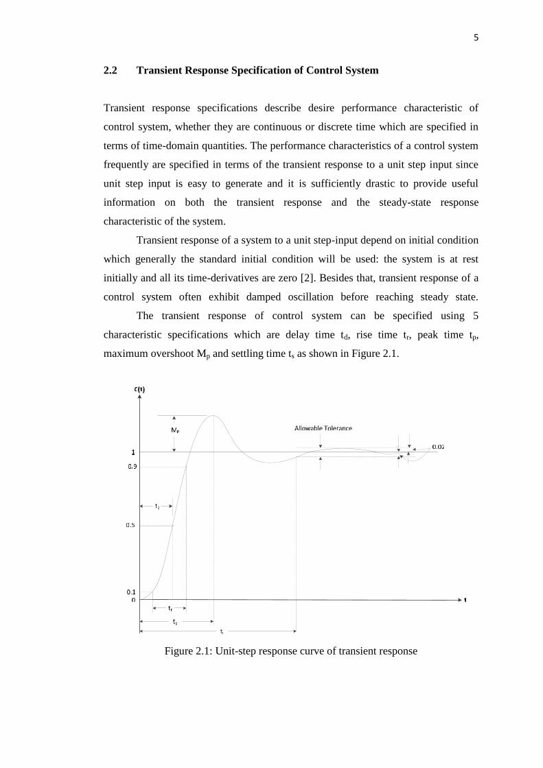
characteristic specifications which are delay time td, rise time tr, peak time tp,

maximum overshoot Mp and settling time ts as shown in Figure 2.1.

Figure 2.1: Unit-step response curve of transient response

6

Figure 2.1 show unit step response curve of transient response specification

td, tr, tp, Mp and ts. The delay time, td can be defined as the time required for the

response to reach half the final value the very first time while the peak time, tp is the

time required for the response to reach the first peak of the overshoot. The rise time,

tr is the time required for the response to rise from 10% to 90%, or 5% to 95% or 0%

to 100%, depending on the situation of the control system. Besides that, the

maximum overshoot, Mp describe the maximum peak value of the response curve

which measured from unity. However, if the final steady-state value of the response

differs from unity, thus it is common to use the maximum percent overshoot which

defined by the relation [2, 26]

ℎ = − (∞)(∞) × 100%The maximum percentage of overshoot directly indicates the relative stability

of the system. The settling time, ts is the time required for the response curve to reach

steady state and stay within a range about the final value of a size specified as an

absolute percentage of the final value, usually 2%.

The transient response specifications of time-domain are quite important

since most of control systems are time domain system. Therefore, the control system

being designed must be modified until the transient response specifications has been

satisfied [2].

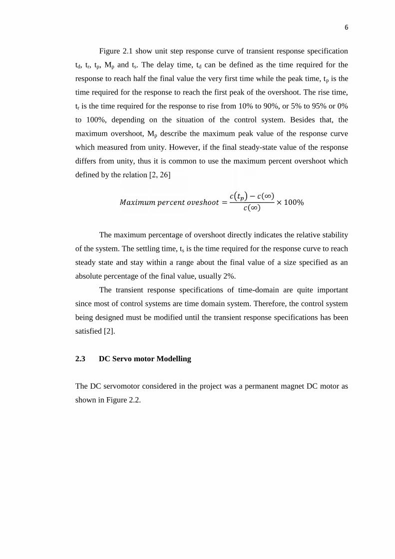
2.3 DC Servo motor Modelling

The DC servomotor considered in the project was a permanent magnet DC motor as

shown in Figure 2.2.

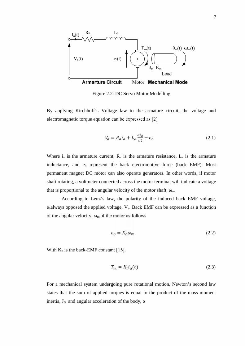
7

Figure 2.2: DC Servo Motor Modelling

By applying Kirchhoff’s Voltage law to the armature circuit, the voltage and

electromagnetic torque equation can be expressed as [2]

= + + (2.1)

Where ia is the armature current, Ra is the armature resistance, La is the armature

inductance, and eb represent the back electromotive force (back EMF). Most

permanent magnet DC motor can also operate generators. In other words, if motor

shaft rotating, a voltmeter connected across the motor terminal will indicate a voltage

that is proportional to the angular velocity of the motor shaft, ωm.

According to Lenz’s law, the polarity of the induced back EMF voltage,

ebalways opposed the applied voltage, Va. Back EMF can be expressed as a function

of the angular velocity, ωm.of the motor as follows

= (2.2)

With Kb is the back-EMF constant [15].

= ( ) (2.3)

For a mechanical system undergoing pure rotational motion, Newton’s second law

states that the sum of applied torques is equal to the product of the mass moment

inertia, JG and angular acceleration of the body, α

8

∑ = (2.4)

In the case of the DC servomotor, JG is equal to the sum if the mass moment

of inertia of the motor armature, Jmand the load, JL with JL usually negligible. The net

torque generated by the motor is equal to motor torque, Tm minus the rotational

viscous friction. The rotational viscous friction associated with the motor is

proportional to the motor angular velocity, ωm.

− = ( + ) (2.5)

− = (2.6)

whereBm is the viscous damping coefficient. Replacing the angular acceleration of

the motor with rate-of change of angular velocity yield:

− = (2.7)

The torque, velocity and position can be related by:

= + (2.8)

= (2.9)

= (2.10)

with TL is the load torque and θm is the motor displacement [1, 2, 5,15, 20].

2.4 Controllability and Observability

The concept of controllability and observability has been introduced by Kalman

Theorem in 1960. The definitions of controllability and observability can be

described as:

9

(i) A system is said to be state controllable if all the modes are affected by

the input vector, otherwise it is not state controllable.

(ii) A system is said to be state observable if all its modes appear at the

output.

Based on Kalman‘s Theorem, concept of controllability and observability can be

simplified as [1, 2, 25, 31]

Theorem 1: A continuous or discrete system is completely state controllable if and

only if the rank of the composite n x nr matrix was

[ ⋮ ⋮ ⋮ ⋯ ⋮ ] = (2.11)

Theorem 2: A continuous or discrete system is completely state observable if and

only if the rank of the composite n x n matrix was

[ ⋮ ⋮ ( ) ⋮ ⋯ ⋮ ( ) ] = (2.12)

2.5 Optimal Control

Optimal control is one particular branch of modern control that sets out to provide

analytical designs system that sets out to provide analytical designs of the system that

is the end result of an optimal design which is not supposed merely to be stable, but

have a certain bandwidth, or satisfy any one of the desirable constraints associated

with classical control. However, it is supposed to be the best possible system of a

particular type which represents the word of optimal. If it is both optimal and

possesses a number of the properties that classical controls suggest are desirable,

hence the controller is much the better [4, 20].

Linear optimal control is a special sort of optimal control where the plant that

is controlled is assumed linear and the controller, the device that generates the

optimal control is also constrained to be linear. Linear controllers are achieved by

following the quadratic performance indices by using linear optimal control which is

termed as Linear Quadratic (LQ) method. The term ‘linear” specified that the

systems considered were assumed linear and the term “quadratic” describe the use of

10

performance measures that involve the square of an error signal. In discrete system

systems, the cost function which is also called the performance index is generally the

form

= ∑ [ ( ), ( ), ( )] (2.13)

In equation (2.13), k known as the sample instant and N is the terminal sample

instant. The control system outputs are y(k), the inputs are r(k) while u(k) are the

control inputs to the plant. The control inputs are always constrained in a physical

system.

Since the quadratic cost function is simpler and the cost function is logical,

thus the design technique for optimal linear regulator control systems based on

quadratic cost functions is developed. This design results in a control law of the form

( ) = − ( ) ( ) (2.14)

where K denoted by full-state feedback gain [1, 2, 3, 4, 5].

2.6 The Quadratic Cost Function

The development of optimal control design begin by considering the case of a

quadratic cost function of the states and the control signals, that is

= ∑ [ ( ) ( ) ( ) + ( ) ( ) ( )] (2.15)

where N is finite and Q(k) and R(k) is symmetric. The linear plant is described by [1,

2]

( + 1) = ( ) ( ) + ( ) ( ) (2.16)( ) = ( ) ( ) + ( ) ( ) (2.17)

where

x(k) = state vector (n-vector)

11

u(k) = control vector (r-vector)

A = n x n system matrix

B = n x r input matrix

C = m x n output matrix

D = m x r connection matrix

2.7 The Principle of Optimality

For a linear discrete plant which has been described in equation (2.16) and (2.17), the

optimal control can be determine by

°( ) = [ ( )] (2.18)

that minimizes the quadratic cost function of equation (2.15)

= 12 [ ( ) ( ) ( ) + ( ) ( ) ( )]where N is finite and Q(k) is positive semi-definite and R(k) is positive definite. In

equation (2.18), the superscript o denotes that the control is optimal. The principle of

optimality may be stated as follows:

If a closed-loop control uo(k) = f[x(k)] is optimal over the interval 0 ≤ k ≤ N, it is

also optimal over any subinterval m ≤ k ≤ N, where 0 ≤ m ≤ N.[1]

The principle of optimality can be defined using scalar Fkas

= ( ) ( ) ( ) + ( ) ( ) ( ) (2.19)

Then, equation (2.13) can be expressed as

= + +⋯+ +

12

Now, let Sm be the cost from k = m to k = N; that is,

= − = + +⋯+ +The principle of optimality states that if JN is the optimal cost, then it also applied to

Sm, for m = 1, 2, …, (N+1). The principle of optimality can be apply by minimizing

S1 = FN, after that FN-1 was choosing to minimize

= + = ° +This step was continuing until SN+1= JN is minimized. The controller that has

been design using this procedure is known as dynamic programming. The general

design procedure will be developed in next section [1, 2, 4].

2.8 Linear Quadratic Optimal Control

Linear Quadratic Optimal Control can be developed based on Quadratic Cost

Function and the principle of optimality. Quadratic optimal control problems can be

solved by many different approaches such as conventional minimization method

using Lagrange multipliers.

A linear discrete plant for linear quadratic optimal was described in equation

(2.16) and (2.17) as

( + 1) = ( ) ( ) + ( ) ( )( ) = ( ) ( ) + ( ) ( )while the optimal control determine by using equation (2.18)

°( ) = [ ( )]that minimizes the quadratic function

= ( ) ( ) + ∑ [ ( ) ( ) ( ) + ( ) ( ) ( )] (2.20)

13

where

Q(k) = n x n positive definite or positive semidefiniteHermitian matrix (or

real symmetrix matrix)

R(k) = r x r positive definite Hermitian matrix (or real symmetric matrix)

S(N) = n x n positive definite or positive semidefiniteHermitian matrix (or

real symmetric matrix)

Matrices Q and R are selected weight the relative importance of the performance

measures caused by state vector x(k) (k = 0, 1, 2, …, N-1), the control vector u(k) (k

= 0, 1, 2, …, N-1) and the final state x(N), respectively. Besides that, N is finite

which make the feedback gain matrix K(k) becomes time-varying matrix [1, 2, 4, 6]

The initial state of this at the system is at some arbitrary state x(0) = c. The

final state x(N) may be fixed, in which case the term ( ) ( ) is removed from

the performance index of Equation (2.20) and instead the terminal condition x(N) =

xfis imposed where xf is the fixed terminal state. If the final state x(N) is not fixed,

then the first term in Equation (2.20) represent the weight of the performance

measure due to the final state. In the minimization problem, the inclusion of the term( ) ( ) in the performance index J implies that the final state x(N) desire to

be as close to the origin as possible [1, 2, 3, 4].

2.9 Steady-State Quadratic Optimal Control

When the control process is finite (when N is finite), the feedback gain matrix K(k)

becomes a time-varying matrix. However, for the quadratic optimal control of an

infinite stage process (where N is infinity), as N approaches infinity the optimal

control solution becomes a steady-state solution and the time-varying gain matrix

K(k) becomes a constant gain matrix. A constant gain matrix K(k) is called a steady-

state gain matrix and can be written as K [1, 2, 3].

In order to solve steady-state quadratic optimal control problem, steady- state

quadratic optimal control of a regulator system has been considered. The plant

equation is given by equation (2.16)

( + 1) = ( ) ( ) + ( ) ( )

14

For N = ∞, the performance index may be modified to

= 12 [ ( ) ( ) ( ) + ( ) ( ) ( )]The term ( ) ( ) which appeared in equation (2.20) is not included because

the optimal regulator system is stable so that the value of JN converges to a constant,

thus x(∞) becomes zero and (∞) (∞) = 0.

Steady-state matrix P(k) was defined as P with P(k) is called as Riccati

Equation

( ) = + ′ ( + 1)[ + ′ ( + 1)] (2.21)

An alternative expression for P can be derived from equation (2.21):

= + ′ − ( + ) ′ (2.22)

Equation (2.22) was defined as Steady-State Riccati Equation. The steady gain

matrix can obtained in terms of P as

= ( + ′ ) ′ (2.23)

The optimal control law for steady-state operation is given by

u(k) = −Kx(k)(2.24)

The performance index associated with the steady-state optimal control law can be

defined as

J = x (0)Px(0) (2.25)

15

In many practical systems, instead of using a time-varying gain matrix K(k), a gain

matrix will be approximate by constant gain matrix K [1, 2, 3]

2.10 State Estimation

State estimation is a technique to estimates the state of a plant from the information

that is available concerning the plant. The system that estimates the state of another

system is generally called observer or state estimator. The plant is described by

equation (2.16) and (2.17) with D(k) = 0

( + 1) = ( ) ( ) + ( ) ( )( ) = ( ) ( )where y(k) are the plant signals that will be measured. The state of the system to be

observed are x(k) and the state of the observer, q(k). Besides that, the desire q(k)

should be approximately equal to x(k). Since the observer will be implemented on a

computer, the signals q(k) are then available for feedback calculations [1, 2]

2.10.1 Observer Model

The observer design criterion to be used is that transfer function matrix from the

input u(k) to the observer state qi(k) be equal to that from the input u(k) to the system

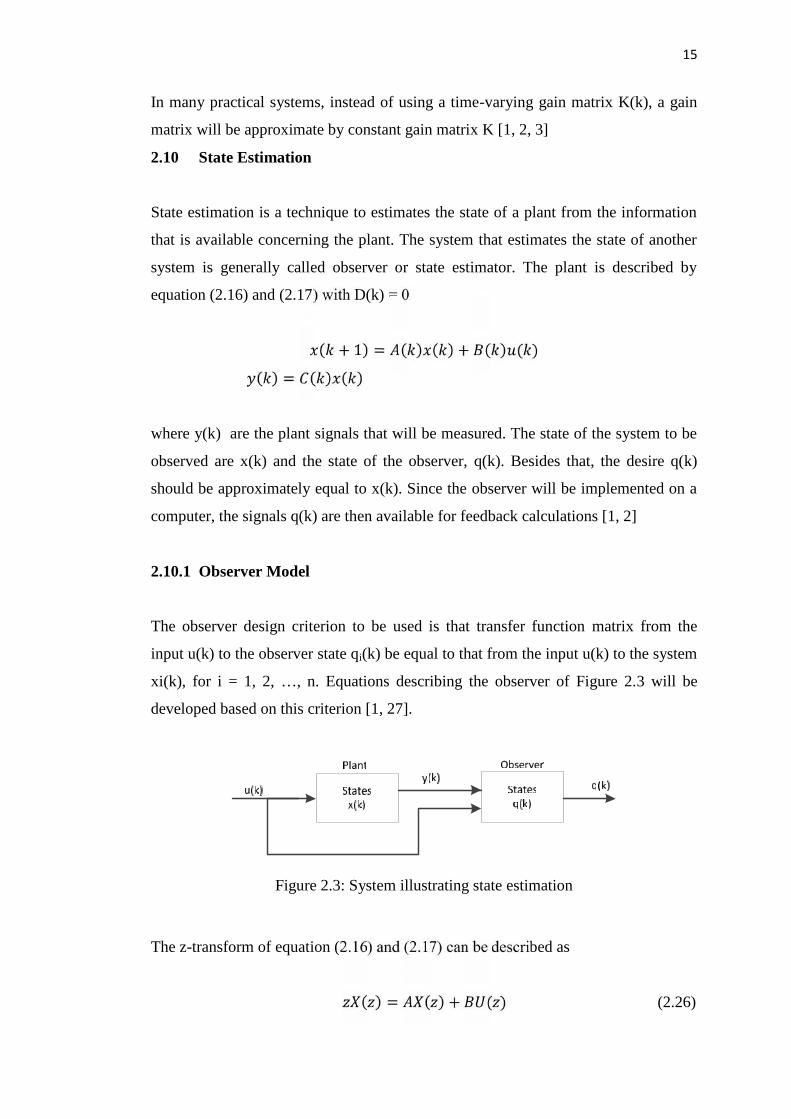
xi(k), for i = 1, 2, …, n. Equations describing the observer of Figure 2.3 will be

developed based on this criterion [1, 27].

Figure 2.3: System illustrating state estimation

The z-transform of equation (2.16) and (2.17) can be described as

( ) = ( ) + ( ) (2.26)

16

( ) = ( ) (2.27)

Thus it can be described that ( ) = ( − ) ( ) (2.28)

Since the observer has two inputs, y(k) and u(k), the observer state equation

can be written as ( + 1) = ( ) + ( ) + ( ) (2.29)

where the matrices F, G and H are unknown. Taking the z-transform of equation

(2.31) and solving Q(z) yields

( ) = ( − ) [ ( ) + ( )] (2.30)

From Equation (2.27) ( ) = ( ) (2.31)

Substitution of equation (2.32) and (2.30) into Equation (2.32) yields:

( ) = ( − ) [ ( ) + ( )]= ( − ) [ ( − ) + ] ( ) (2.32)

Recall that based on design criterion, the transfer function matrix from U(z)

to Q(z) same as from U(z) to X(z). Therefore equation (2.30) become

( ) = ( − ) ( ) (2.33)

Then, from equation (2.33) and (2.34)

( − ) = ( − ) [ ( − ) + ]( − ) = ( − ) ( − ) + ( − )or [ − ( − ) ]( − ) = ( − )

17

This equation can be expressed as( − ) [ − ( + )]( − ) = ( − )Equating the post multiplying matrices of ( − ) yields

( − ) = [ − ( + )] (2.34)

This equation is satisfied when H equal to B and

= + (2.35)

Therefore, from equation (2.35), the observer state equation can be written as

( + 1) = ( − ) ( ) + ( ) + ( ) (2.36)

and the design criterion of equation (2.34) is satisfied. Since G is unspecified, hence

the observer is a dynamic system described by Equation (2.36) with y(k) and u(k) as

inputs and with the characteristic equation

| − + | = 0 (2.37)

The observer state equation is known as prediction observer, since the

estimate at time (k+1)T is based on the measurement at time kT[1, 2, 4, 6].

2.10.2 Errors in Estimation

The error vector, e(k) in the state-estimation process is define as

( ) = ( ) − ( ) (2.38)

Then, from equation (2.16), (2.17) and (2.37), equation (2.38) can also be describe as

18

( + 1) = ( + 1) − ( + 1)= ( ) + ( ) − ( − ) ( ) − ( ) − ( ) (2.39)

or ( + 1) = ( − )[ ( ) − ( )] = ( − ) ( ) (2.40)

Hence, the error dynamics have a characteristic equation given by

| − ( − )| = 0 (2.41)

which is similar to equation (2.38).

The errors in state estimation may occur due to the choice of initial conditions

for the observer. Since the initial states of the plant will not be known, thus the initial

error e(0) will not be zero. However, since the provided observer is stable, this error

will tend to zero with increasing time.

Besides that, the errors in state estimation can be also due to the plant

disturbances and the sensor errors. The complete state equation of the plant in

equation (2.16) and (2.17) become

( + 1) = ( ) ( ) + ( ) ( ) + ( ) (2.42) ( ) =( ) ( ) + ( ) ( ) + ( ) (2.43)

When the plant disturbance vector w(k) and the measurement inaccuracies v(k) are

considered. Hence, if equation (2.42) and (2.43) is used in deriving the error state

equations, Equation (2.40) can be describe as

( + 1) = ( − ) ( ) + ( ) − ( ) (2.44)

For this case, the errors in the state estimation will tend to zero if the estimator is

stable. However, the excitation terms in Equation (2.44) will prevent the errors from

reaching a value of zero. Therefore, optimal state estimation by using Kalman

filtering will be considered to ensure the errors in state estimation become zero [1,2].

2.11 Optimal State Estimation – Kalman Filters.

19

The plant is assumed to be described as

( + 1) = ( ) ( ) + ( ) ( ) + ( )( ) = ( ) ( ) + ( ) ( ) + ( )where x(k) [n x 1] are the states, u(k) [r x 1] are the known inputs, w(k) [s x 1] are

the random plant disturbances, y(k) [p x 1] are the measurement and v(k) [p x 1] are

the random inaccuracies in the measurement [1,2]

The random inputs w(k) and v(k) in equation (2.42) and (2.43) are assumed to

be uncorrelated and to have Gaussian distributions with the properties:

[ ( )] = 0, [ ( )] = 0[ ( ), ( )] = [ ( ) ( ) = (2.45)[ ( ), ( )] = [ ( ) ( ) =with E[.] is the mathematical expectation operation and cov[.] denotes the covariance

[16, 22, 23]. Besides that, is the Kronecker delta function, defined by

= 0, ≠1, =Hence w(k) and v(k) are discrete white-noise sequence with Gaussian distributions.

The error estimation has been described by equation (2.38)

( ) = ( ) − ( )The covariance of the vector is denoted as P(k)[n x n], with

( ) = [ ( ) ( )] (2.46)

where the diagonal elements of P(k) are the average square errors of the estimation.

The cost function for the minimization process is chosen as the trace of P(k) which is

the sum of the diagonal elements or the sum of the average squared errors of

estimation.

20

( ) = ( ) = [ ( )] + [ ( )] +⋯+ [ ( )]= ( ) + ( ) +⋯+ ( ) (2.47)

Where ( )is the variance of ( ). This cost function can also be expressed as

( ) = [ ( ) ( )]Since the system of equation (2.42) and (2.43) has random inputs and the

measurements have random error, so the actual estimation errors can never be

determined [24]. Hence, only the statistical characteristics of the estimation errors

will be considered, and minimize a function of the expected values of these errors.

Hence the Kalman filter is optimal only on the average [1, 24].

Besides that, an additional property of the Kalman filter is the cost function

′( ) = [ ( ) ( )] (2.48)

with J’(k) is minimized for any Q positive semidefinite matrix. Hence the sum of

cost function can be describe as

= [ ( )] + [ ( )] = [ ( ) ( )]will is also minimized. The mathematical development requirement to minimize the

cost function resulting Kalman filter equation as

( ) = ( ) + ( )[ ( ) − ( )] (2.49)( + 1) = ( ) + ( ) (2.50)

where ( ) is the predicted state estimate at the sampling instant k, and q(k)is the

actual state estimate at k. The gain matrix G(k) is the Kalman gain, and is calculated

from the covariance equations

( ) = ( ) [ ( ) + ]

21

( ) = ( ) − ( ) ( ) (2.51)( + 1) = ( ) +with M(k) is known as covariance of the prediction errors:

( ) = {[ ( ) − ( )][ ( ) − ( )] } (2.51)

while P(k) is defined in equation (2.46). The second equation in (2.51) can be

substituted into the third equation of equation (2.51) to expressed as a single

difference equation in M(k).

( + 1) = [ − ( ) ] ( ) + (2.52)

In steady-state Kalman filter case, G(k) becomes constant and the filter equation

(2.48) has the characteristic equation [1, 2]

| − ( − )| = 02.11.1 The Discrete Kalman Filter Algorithm

In the discrete Kalman filter algorithm, Kalman filter estimates the process by using

a form of feedback control. The filter estimates the process state at some time and

then obtains the feedback in the form of noise measurement. Kalman filter can be

divided into two groups which are time update equations and measurement update

equations.

22

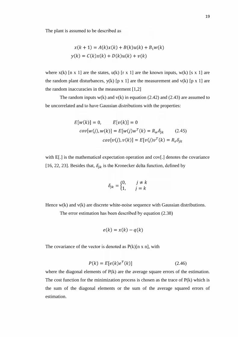
Figure 2.4: Discrete Kalman Filter process

Figure 2.4 show the operation of Kalman filter. The operation can be

described in two terms which are time update equations and measurement update

equations.The time update equations are to update the current error covariance

estimation to obtain the estimation of a priori for the next time step. The

measurement update equations are responsible for the feedback such as for

incorporating a new measurement into the a priori estimate to obtain an improved a

posteriori estimate. Time update can also be thought of as a predictor equation while

the measurement update can be thought as corrector equation [1, 16].

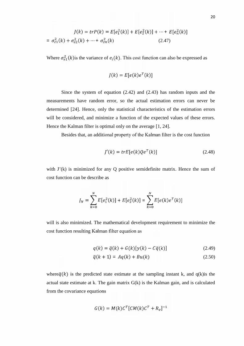
2.12 Linear Quadratic Gaussian (LQG)

Figure 2.5: LQG Control System

Figure 2.5 show the block diagram of LQG control system which has been

derived from equation (2.49) and (2.50). Figure 2.5 describe LQG control system can

be implement by using Linear Quadratic (LQ) optimal control and Kalman filter

23

which Kalman filter will be act as estimator. Besides that, the implementation of full-

state feedback control systems using Kalman filters as state estimators can also result

in systems that are not robust.Hence the control-estimator transfer function, Dce(z)

will be determined by simplify the block diagram of Figure 2.5 which can be

performed with DARE [1]. Combination of the control-estimator transfer function

also known as LQG digital controller transfer function, GD(z).

Since LQG is implemented based on LQ optimal control and Kalman filter,

hence Separation Principle will be used. The Separation Principle is utilized in the

LQG design as a two-step process

Step 1. Obtain the optimal state-feedback matrix gain (K) based on Steady-State

Quadratic Optimal Control (Section 2.9).

= ( + ′ ) ′Step 2.Obtain the Kalman Filter gain matrix (G) by using Optimal State Estimation

method (Section 2.11)

( ) = ( ) [ ( ) + ]2.13 Matrix Laboratory (MATLAB)

MATLAB is a high-level language and interactive environment that has been

developed by MathWorks for numerical computation, visualization and

programming. MATLAB allows matrix manipulations, plotting of functions and data

implementation of algorithm, creation of user interfaces and interfacing with

programs written in other language including C, C++, Java and FORTRAN.

The MATLAB application is built around the MATLAB language and most

use of MATLAB involves typing MATLAB code into the Command Window or

executing text file containing MATLAB code and functions. However as the number

of command increases or trial and error is done by changing certain variable, M-files

will be helpful to run the command efficiently.An m-file or scrip file is a simple text

file to place MATLAB commands

MATLAB also supports developing application with graphical interface

features. MATLAB includes GUIDE (GUI development environment) for graphical

24

designing GUIs. Besides that, MATLAB also supports Simulation and Model-Based

Design (Simulink). Simulink is a block diagram environment for multidomain

simulation and Model-Based Design. It provides a graphical editor, customizable

block libraries and solvers for modeling and simulating dynamic system.

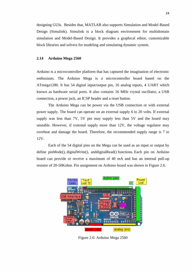
2.14 Arduino Mega 2560

Arduino is a microcontroller platform that has captured the imagination of electronic

enthusiasts. The Arduino Mega is a microcontroller board based on the

ATmega1280. It has 54 digital input/output pin, 16 analog inputs, 4 UART which

known as hardware serial ports. It also contains 16 MHz crystal oscillator, a USB

connection, a power jack, an ICSP header and a reset button.

The Arduino Mega can be power via the USB connection or with external

power supply. The board can operate on an external supply 6 to 20 volts. If external

supply was less than 7V, 5V pin may supply less than 5V and the board may

unstable. However, if external supply more than 12V, the voltage regulator may

overheat and damage the board. Therefore, the recommended supply range is 7 to

12V.

Each of the 54 digital pins on the Mega can be used as an input or output by

define pinMode(), digitalWrite(), anddigitalRead() functions. Each pin on Arduino

board can provide or receive a maximum of 40 mA and has an internal pull-up

resistor of 20-50Kohm. Pin assignment on Arduino board was shown in Figure 2.6.

Figure 2.6: Arduino Mega 2560

94

REFERENCES

[1] Charles L. Phillips and H. Troy Nagle, Digital Control System Analysis and

Design.3rd ed. New Jersey, USA.: Prentice Hall. 1998

[2] Katsuhiko Ogata, Discrete-Time Control Systems. 2nd ed. New Jersey, USA.:

Prentice Hall. 1994.

[3] Frank L. Lewis, Draguna L. VrabieandVassilis L. Syrmos, Optimal Control.

3rded. New Jersey, USA: John Wiley and Sons. 2012

[4] Brian D.O Anderson & John B. Moore, Thomas Kailath (Ed.), Optimal

Control Linear Quadratic Methods.New Jersey, USA.: Prentice Hall. 2012

[5] Elbert Hendricks, Ole Jannerupand Paul Haase Sorensen, Linear System

Control Deterministic and Stochastic Methods. Denmark.: Springer. 2008

[6] Peter Dorato, ChaoukiAbdallahand Vito Cerone (Ed.), Linear Quadratic

Control: An Introduction. New Jersey, USA: Prentice Hall. 1995.

[7] Simon Monk, Programming Arduino: Getting Started with

Sketch.USA.:McGraw-Hill. 2012.

[8] ShamsulNizambinMohdYusof @ Hamid, Developing LQR to Control Speed

Motor using Matlab GUI.Bachelor Thesis.Universiti Malaysia Pahang: 2008.

[9] PhongsakPhakamatch, Control of a DC Servo Motor using Fuzzy Logic

Sliding Mode Model Following Controller. Proceeding of the World

Academy of Science, Engineering and Technology 60 2009, pp. 504-509

[10] Rene Barera-Cardenas and Marta Molinas.Optimal, LQG Controller for

Variable Speed Wind Turbine based on Genetic Algorithm. Proceeding of the

Energy Proceedia 20(2012),pp. 207-216.

[11] E. Maneri and W. Gawronski.LQG Controller Design using a Graphical

User Interface (GUI). Bachelor Thesis.Montana State University, Bozeman.

2000.

95

[12] Gianni Ferreti, Gian Antonio Magnani and Paolo Rocco.LQG Control of

Elastic Servomechanism based on Motor Position Measurement.Bachelor

Thesis. Milano Polytechnic: 1998

[13] Jium-Ming Lin, Hsiu-Ping Wang and Ming-Chang Lin.LEQG/LTR

Controller Design with Extended Kalman Filter for Sensorless Induction

Motor Servo Drive. Proceeding of the ICAS 2000 Congress, 634.1-634.10.

[14] WaiPhyoAung, Analysis on Modeling and Simulink of DC Motor and its

Driving System used for Wheeled Mobile Robot.International Journal of

Computer and Information Engineering 2:1 2008, 22-29.Retrieved from

https://www.waset.org/journals/ijcie/v2/v2-1-4.pdf.

[15] AamirHashim Obeid Ahmed, Optimal Speed control for Direct Current

Motors using Linear Quadratic Regulator.International Journal of Science

and Technology vol 13 2012.Retrived from www.sustech.edu.

[16] Greg Welch and Gary Bishop, An Introduction to the Kalman Filter.

Proceeding SIGGRAPH 2001, 1-80.

[17] Lab-Volt Ltd. Digital Servo Motor Control – Student Manual. Canada: Lab-

Volt Ltd. 2010.

[18] Reston Condit Microchip Technology Inc. Brushed DC Motor Fundamentals.

Reston Condit Microchip Technology Inc. 2004.

[19] I.Robadi, K. Nishimori, R. Nishimura, N. Ishirah. Optimal Feedback Control

Design using Power System. Electrical Power and Energy System 23, pp.

263-271, 2001

[20] R. Yu, R. Hwang. OptimalPID Speed Control of Brushless DC Motors using

LQR Approach. Proceeding ofIEEE International Conference on Man and

Cybernetics, Hague.Netherlands, October 2004.

[21] P.O.M. Scokaert and J. B. Rawlings.Constrained Linear Quadratic

Regulation, IEEE Transactions Automatic Control, Vol. 43, No. 8, pp. 1163-

1169, 1998.

[22] J. C. Doyle and G. Stein, Multivariable Feedback Design: Concepts for a

Classical/Modern Synthesis. IEEE Transactions on Automatic Control, vol.

AC-26, No. 1, 1981, pp. 4-16.

[23] G. Stein and M. Athans. The LQR/LTR procedure for multivariable feedback

control design. IEEE Transactions on Automatic Control, vol. 32, Feb, 1987,

pp. 105-106.

96

[24] Michael Athans.The Role and Use of the Stochastic Linear-Quadratic

Gaussian Problem in Control System Design.IEEE Transactions on

Automatic Control, vol. AC-16, No. 6. Dec, 1971, pp. 529-552.

[25] Kreindler, E. and P. E. Sarachik.The Concepts of Controllability and

Observability of Linear System, IEEE Transactions Automatic Control, AC-9

(1964), pp. 129-136.

[26] Kuo, B. C. Digital Control System. New York: Holt, Rinehart and Winston,

Inc., 1980

[27] Luenberger, D. G. An Introduction to Observers. IEEE Transactions

Automatic Control, AC-16 (1971), pp. 596-602

[28] Katsuhiko Ogata, Solving Engineering Problem with MATLAB. Eaglewood

Cliffs, N. J.: Prentice Hall, Inc., 1994.

[29] Payne, H, H. J. and L. M. Silverman, The Discrete Time Algebraic Riccati

Equation. IEEE Transaction Automatic Control, AC-18 (1973), pp. 226-234.

[30] Zadeh, L. A., and C. A. Desoer.Linear System Theory: The State Space

Approach. New York: McGraw-Hill Book Company, 1963.

[31] Wilems, J. C., and S. K. Mitter. Controllability, Observability, Pole

Allocation and State Reconstruction, IEEE Transactions Automatic Control,

AC-16 (1971), pp. 582-595.

linear quadratic gaussian (lqg) c ontroller design...

Documents