line integrals and green’s theorem jeremy orlojorloff/18.04/notes/greenstheorem.pdf · line...

Line Integrals and Green’s TheoremJeremy Orloff

1 Vector Fields (or vector valued functions)

Vector notation. In 18.04 we will mostly use the notation (v) = (a, b) for vectors. Theother common notation (v) = ai + bj runs the risk of i being confused with i =

√−1

–especially if I forget to make i boldfaced.

Definition. A vector field (also called called a vector-valued function) is a function F(x, y)from R2 to R2. That is,

F(x, y) = (M(x, y), N(x, y)),

where M and N are regular functions on the plane. In standard physics notation

F(x, y) = M(x, y)i +N(x, y)j = (M,N) .

Algebraically, a vector field is nothing more than two ordinary functions of two variables.

Example GT.1. Here are a number of standard examples of vector fields.

(a.1) Force: constant gravitational field F(x, y) = (0,−g).

(a.2) Velocity:

V(x, y) =

(x

x2 + y2,

y

x2 + y2

)=( xr2,y

r2

).

(Here r is our usual polar r.) It is a radial vector field, i.e. it points radially away from theorigin. It is a shrinking radial field –like water pouring from a source at (0,0).

This vector field exhibits another important feature for us: it is not defined at the originbecause the denominator becomes zero there. We will say that V has a singularity at theorigin.

(a.3) Unit tangential field: F = (−y, x) /r. Tangential means tangent to circles centeredat the origin. We know it is tangential because it is orthogonal to the radial vector field in(a.2). F also has a singularity at the origin. We

(a.4) Gradient field: F = ∇f , e.g., f(x, y) = xy2 ⇒ ∇f =(y2, 2xy

).

1.1 Visualization of vector fields

This can be summarized as: draw little arrows in the plane. More specifically, for a field F,at each of a number of points (x, y) draw the vector F(x, y)

Example GT.2. Sketch the vector fields, (a.1), (a.2) and (a.3) from the previous example.

1

2 DEFINITION AND COMPUTATION OF LINE INTEGRALS ALONGA PARAMETRIZED CURVE2

x

y

(a.1) Constant vector field

x

y

(a.2) Shrinking radial field

x

y

(a.3) Unit tangential field

2 Definition and computation of line integrals along a parametrizedcurve

Line integrals are also called path or contour integrals.

We need the following ingredients:

A vector field F(x, y) = (M,N)

A parametrized curve C: r(t) = (x(t), y(t)), with t running from a to b.

Note: since r = (x, y), we have dr = (dx, dy).

Definition. The line integral of F along C is defined as

∫

CF · dr =

∫

C(M,N) · (dx, dy) =

∫

CM dx+N dy.

Comment: The notation F · dr is common in physics and M dx+N dy in thermodynamics.(Though everyone uses both notations.)

We’ll see what these notations mean in practice with some examples.

Example GT.3. Let F(x, y) =(x2y, x− 2y

)and let C be the curve r(t) =

(t, t2

), with t

running from 0 to 1. Compute the line integral I =

∫

CF · dr.

Do this first using the notation

∫

CM dx + N dy. Then repeat the computation using the

notation

∫

CF · dr.

answer: First we draw the curve, which is the part of the parabola y = x2 running from(0, 0) to (1, 1).

3 WORK DONE BY A FORCE ALONG A CURVE 3

x

y

C

1

1

(i) Using the notation

∫

CM dx+N dy.

We have r = (x, y), so x = t, y = t2. In this notation F = (M, N), so M = x2y andN = x− 2y.

We put everything in terms of t:

dx = dt

dy = 2t dt

M = (t2)(t2) = t4

N = t− 2t2

Now we can put all of these in the integral. Since t runs from 0 to 1, these are our limits.

I =

∫

CM dx+N dy =

∫ 1

0t4 dt+ (t− 2t2)2t dt =

∫ 1

0t4 + 2t2 − 4t3 dt = − 2

15.

(ii) Using the notation

∫

CF · dr.

Again, we have to put everything in terms of t:

F = (M, N) =(t4, t− 2t2

)

dr

dt= (1, 2t) , so d r =

dr

dtdt = (1, 2t) dt

Thus, F · dr =(t4, t− 2t2

)· (1, 2t) dt = t4 + (t− 2t2)2t dt. So the integral becomes

I =

∫

CF · dr =

∫ 1

0t4 + (t− 2t2)2t dt.

This is exactly the same integral as in method (i).

3 Work done by a force along a curve

Having seen that line integrals are not unpleasant to compute, we will now try to motivateour interest in doing so. We will see that the work done by a force moving a body along apath is naturally computed as a line integral.

Similar to integrals we’ve seen before, the work integral will be constructed by dividing thepath into little pieces. The work on each piece will come from a basic formula and the totalwork will be the ‘sum’ over all the pieces, i.e. an integral.

3 WORK DONE BY A FORCE ALONG A CURVE 4

3.1 Basic formula: work done by a constant force along a small line

We’ll start with the simplest situation: a constant force F pushes a body a distance ∆salong a straight line. Our goal is to compute the work done by the force.

The figure shows the force F which pushes the body a distance ∆s along a line in thedirection of the unit vector T̂. The angle between the force F and the direction T̂ is θ.

T̂=unit vector

length=∆s vector=∆r = ∆s T̂

F

θ

We know from physics that the work done by the force on the body is the component ofthe force in the direction of motion times the distance moved. That is,

work = |F| cos(θ) ∆s

We want to phrase this in terms of vectors. Since |T̂| = 1 we know F · T̂ = |F| cos(θ). Usingthis in the formula for work we have

work = F · T̂ ∆s. (1)

Equation 1 is important and we will see it again. For now, we want to make one moresubstitution. We’ll call the vector ∆s T̂ = ∆r. This is the displacement of the body. (Note,

it is essentially the same as our formulads

dtT̂ =

dr

dt.) Using this, Equation 1 becomes

work = F ·∆r. (2)

This is the basic work formula that we’ll use to compute work along an entire curve

3.2 Work done by a variable force along an entire curve

Now suppose a variable force F moves a body along a curve C. Our goal is to compute thetotal work done by the force.

The figure shows the curve broken into 5 small pieces, the jth piece has displacement ∆rj.If the pieces are small enough, then the force on the jth piece is approximately constant.This is shown as Fj .

∆r1

∆r2

∆r3

∆r4

∆r5

F1F2

F3F4

F5

4 GRAD, CURL AND DIV 5

Also, if the pieces are small enough, then each segment is approximately a straight lineand the force is approximately constant. So we can apply our basic formula for work andapproximate the work done by the force moving the body along the jth piece as

∆Wj ≈ Fj ·∆rj .

The total work is the sum of the work over each piece.

total work =∑

∆Wj ≈∑

Fj ·∆rj .

Now, as usual, we let the pieces get infinitesimally small, so the sum becomes an integraland the approximation becomes exact. We get:

total work =

∫

CF · dr.

The subscript C indicates that it is the curve that has been split into pieces. That is, thetotal work is computed as a line integral of the force over the curve C!

4 Grad, curl and div

Gradient. For a function f(x, y): gradf = ∇f = (fx, fy).

Curl. For a vector in the plane F(x, y) = (M(x, y), N(x, y)) we define

curlF = Nx −My.

NOTE. This is a scalar. In general, the curl of a vector field is another vector field. Forvectors fields in the plane the curl is always in the k̂ direction, so we simply drop the k̂ andmake curl a scalar. Sometimes it is called the ‘baby curl’.

Divergence. The divergence of the vector field F = (M,N) is

divF = Mx +Ny.

5 Properties of line integrals

In this section we will uncover some properties of line integrals by working some examples.

Example GT.4. First look back at the value found in Example GT.3. Now, use the samevector field as in that example, but, in this case, let C be the straight line from (0, 0) to

(1, 1), i.e. same endpoints, but different path. Compute the line integral

∫

CF · dr.

answer: As always, start by sketching the curve:

x

y

C

1

1

5 PROPERTIES OF LINE INTEGRALS 6

We’ll use the notation

∫

CM dx+N dy.

Parametrize the curve: x = t, y = t, with t from 0 to 1.

Put everything in terms of t:

dx = dt

dy = dt

M = x2y = t3

N = x− 2y = −t

Now we put this into the integral

I =

∫

CM dx+N dy =

∫ 1

0t3 dt− t dt =

∫ 1

0t3 − t dt = −1

4.

This is a different value from Example GT.3, which leads to the important principle:

Important principle for line integrals. Line integrals over two different paths with thesame endpoints may be different.

Example GT.5. Again, look back at the value found in Example GT.3. Now, use the samevector field and curve as Example GT.3 except use the following (different) parametrizationof C.

x = sin(t), y = sin2(t); 0 ≤ t ≤ π/2.

Compute the line integral

∫

CF · dr.

answer: We won’t sketch the curve it is identical to the one in Example GT.3. Puttingeverything in terms of t we have

dx = cos(t) dt

dy = 2 sin(t) cos(t) dt

M = x2y = sin2(t) sin2(t) = sin4(t)

N = x− 2y = sin(t)− 2 sin2(t)

We put these in the integral I =

∫

CM dx+N dy and compute

I =

∫ π/2

0sin4(t) cos(t) dt+ (sin(t)− 2 sin2(t))2 sin(t) cos(t) dt

=

∫ π/2

0

(sin4(t) + 2 sin2(t)− 4 sin3(t)

)cos(t) dt

(Let u = sin(t), du = cos(t) dt.)

=

∫ 1

0u4 + 2u2 − 4u3 du

= − 2

15.

5 PROPERTIES OF LINE INTEGRALS 7

This is the same value we got in Example GT.3! In fact, the u substitution led to exactlythe same integral! This leads us to the important principle:

Important principle for line integrals. The parametrization of the curve doesn’t affectthe value of line the integral over the curve.

You should note that our work with work make this reasonable, since we developed the lineintegral abstractly, without any reference to a parametrization.

5.1 List of properties of line integrals

1. Independent of parametrization: The value of the line integral

∫

CF · dr is indepen-

dent of the parametrization of C.

2. Reversing direction on the curve changes the sign: If C is a curve, then we write−C for the same curve traversed in the opposite direction. In this case

∫

−CF · dr = −

∫

CF · dr.

(See the next example.)

Example GT.6. Let C be the curve from Example GT.3. Sketch C and −C and give aparametrization of −C.

answer: C follows the parabola y = x2 from (0,0) to (1,1), so the curve −C covers thesame section of the parabola, but goes from (1,1) to (0,0), i.e. we reversed the direction ofthe arrow.

x

y

C

1

1C goes from (0,0) to (1,1)

x

y

−C

1

1−C goes from (1,1) to (0,0)

The curve C can be parametrized as r(t) =(t, t2

), with t running from 0 to 1. The easiest

way to reverse this is to have t run from 1 to 0

With this parametrization the t limits on the integral are reversed, which, we know from18.01, changes the sign of the integral.

If you insist on an increasing parameter, we can parametrize −C by

r(u) =(1− u, (1− u)2

), with u runnning from 0 to 1.

3. (Intrinsic formula) We can write the line integral as∫

CF · dr =

∫

CF ·T ds

where T = unit tangent vector to C and ds = differential of arclength.

6 RECTANGULAR AND CIRCULAR PATHS 8

Reason: We know from our work on parametrized curves thatdr

dt= T

ds

dt. So, dr = T ds.

(A comparison of Equations 1 and 2 above, essentially shows the same thing.)

4. If C is a closed curve we use the notation∮

CF · dr =

∮

CM dx+N dy.

The little circle on the integral sign indicates the curve is closed, i.e. starts and ends at thesame point.

6 Rectangular and circular paths

Example GT.7. Evaluate I =

∫

Cy dx + (x + 2y) dy where C is the rectangular path

from (0,1) to (1,0) shown below.

x

yC1

C2

(1, 1)1

1

answer: The path C is given in two pieces labeled C1 and C2. This means we will have tosplit the integral into two pieces, i.e.

I =

∫

Cy dx+ (x+ 2y) dy =

∫

C1

y dx+ (x+ 2y) dy +

∫

C2

y dx+ (x+ 2y) dy.

We’ll do the integration one piece at a time. First,∫C1y dx+ (x+ 2y) dy.

Parametrize C1: We’ll use x as the parameter:

x = x, y = 1, with x running from 0 to 1

Put everything in terms of x:

x = x, y = 1, dx = dx, dy = 0, M = y − 1, N (skip, since dy = 0).

Put this in the integral and compute:

∫

C1

M dx+N dy =

∫

C1

M dx =

∫ 1

0dx = 1.

Next, the integral over C2.

Parametrize C2: Use parameter y: x = 1, y = y, y runs from 1 to 0.

Put everything in terms of y:

x = 1, y = y, dx = 0, dy = dy, M (skip, since dx = 0), N = x+ 2y = 1 + 2y

7 SOME SUPER-DUPER, REALLY SERIOUSLY IMPORTANT EXAMPLES 9

Put this in the integral and compute

∫

C2

M dx+N dy =

∫

C2

N dy =

∫ 0

11 + 2y dy = −2.

Adding, the pieces we have I = 1− 2 = −1.

Shorthand. Because dy = 0 on C1 and dx = 0 on C2 we can write

∫

C1+C2

M dx+N dy =

∫

C1

M dx+

∫

C2

N dy.

Using the shorthand will save us some writing in the future.

Example GT.8. Evaluate I =

∮

C−y dx+ x dy where C is the unit circle traversed in a

counterclockwise (CCW) direction.

answer: Parametrization: x = cos(t), y = sin(t), 0 ≤ t ≤ 2π. So, dx = cos(t) dt, dy =− sin(t) dt. We get

I =

∫ 2π

0− sin t(− sin t) dt+ cos t(cos t) dt =

∫ 2π

0dt = 2π.

x

y1

1

7 Some super-duper, really seriously important examples

In these examples we are going to integrate a tangential field around a closed loop. Thesewill be key computations as we explore Green’s theorem and gradient fields.

In the following r is the usual polar distance r2 = x2 + y2.

Example GT.9. Let F =⟨− yr2, xr2

⟩, and let C be the unit circle traversed in a counter-

clockwise (CCW) direction. Compute I =

∮

CF · dr

answer: Sketch C and the vector field F.

7 SOME SUPER-DUPER, REALLY SERIOUSLY IMPORTANT EXAMPLES 10

x

y

1

1

Parametrize C: x = cos(t), y = sin(t), 0 ≤ t ≤ 2π.

Put everything in terms of t: (Note, on the unit circle r = 1.)

dx = cos(t) dt, dy = − sin(t) dt, M = − y

r2= − sin(t), N =

x

r2= cos(t).

Put this in the integral and compute:

I =

∫ 2π

0− sin(t)(− sin(t)) dt+ cos(t)(cos(t)) dt =

∫ 2π

0sin2(t) + cos2(t) dt =

∫ 2π

0dt = 2π.

Example GT.10. Let F be the same as the previous example. Let C2 be the unit circle

centered on (2,0) traversed counterclockwise. Compute I2 =

∫

C2

F · dr.

answer: Parametrize C2: x = 2 + cos(t), y = sin(t), t from 0 to 2π.

Put everything in terms of t: (Note, r2 is not constant.)

dx = − sin(t) dt

dy = cos(t) dt

r2 = x2 + y2 = (2 + cos(t))2 + sin2(t) = 5 + 4 cos(t)

M = − y

r2= − sin(t)

5 + 4 cos(t)

N =x

r2=

2 + cos(t)

5 + 4 cos(t)

Put this in the integral:

I2 =

∫

C2

M dx+N dy =

∫ 2π

0

sin2(t) + 2 cos(t) + cos2(t)

5 + 4 cos(t)dt =

∫ 2π

0

1 + 2 cos(t)

5 + 4 cos(t)dt

Oy! We put this into Wolfram Alpha and found I2 = 0.

Note. We should suspect that the value of 0 is no accident. This is true and we will seeit easily once we learn Green’s theorem. Avoiding actually computing an integral like thisshould be motivation enough for us to learn Green’s theorem.

18.01 challenge. Compute the integral for I2. Hints: You can use the substitutionu = tan(t/2) and partial fractions. It’s best to use symmetry and compute 2 times theintegral from 0 to π.

8 GRADIENT AND CONSERVATIVE FIELDS 11

8 Gradient and conservative fields

We will now focus on the important case where F is a gradient field. That is, for somefunction f(x, y),

F = ∇f = (fx, fy) .

Note. We will learn to call f a potential function for F.

8.1 The fundamental theorem for gradient fields

Theorem GT.11. (fundamental theorem for gradient fields) Suppose that F = ∇f is agradient field and C is any path from point P to point Q. The fundamental theorem forvector fields says

∫

CF · dr = f(x, y)|QP = f(Q)− f(P ) = f(x1, y1)− f(x0, y0). (3)

where P = (x0, y0) and Q = (x1, y1).

That is, for gradient fields the line integral depends only on the endpoints of the path andis independent of the path taken.

x

y

C1

P = (x0, y0)

Q = (x1, y1)C2

If F = ∇f then

∫

C1

F · dr =

∫

C2

F · dr = f(Q)− f(P ).

The proof of the fundamental theorem is given after the next example

Example GT.12. Let f(x, y) = xy3+x2 and let C be the curve shown. Compute F = ∇f

and compute

∫

CF · dr two ways: (i) directly as a line integral, (ii) using the fundamental

theorem.

x

y

C

(0, 0)

(1, 2)


answer: F(x, y) = ∇f (fx, fy) =(y3 + 2x, 3xy2

)

(i) Parametrize C: x = t, y = 2t, t runs from 0 to 1.

Write everything in terms of t:

dx = dt, dy = 2 dt, M = y3 + 2x = 8t3 + 2t, M = 3xy2 = 12t3.

Put all this into the integral and compute:

∫

CF · dr =

∫

C(y3 + 2x) dx+ 3xy2 dy =

∫ 1

0(8t3 + 2t) dt+ 12t32 dt =

∫ 1

032t3 + 2t dt = 9.

(ii) By the fundamental theorem

∫

CF · dr =

∫

C∇f · dr = f(1, 2)− f(0, 0) = 9.

You decide which method is easier!

8.2 Proof of the fundamental theorem

Proof. The proof uses the definition of line integral together with the chain rule and theusual fundamental theorem of calculus.

We assume the following:(i) F = ∇f(ii) The curve C is parametrized by r(t) = (x(t), y(t)), with t running from t0 to t1 andr(t0) = P , r(t1) = Q.

First recall the for a parametrized curve r(t) the chain rule says

df(r(t))

dt= fx

dx

dt+ fy

dy

dt= ∇f · dr

dt.

So,

∫

CF · dr =

∫

C∇f · dr =

∫ t1

t0

∇f · drdtdt =

∫ t1

t0

df(r(t))

dtdt

= f(r(t))|t1t0 = f(r(t1))− f(r(t0)) = f(Q)− f(P ) QED

8.3 Path independence

Definition. For a vector field F we say that the line integrals

∫

CF·dr are path independent

if for any two points P and Q the integral yields the same value for every path connectingP to Q.

From the fundamental theorem we can conclude: if F = ∇f is a gradient field, then the

integrals

∫

CF · dr are path independent.


The following theorem offers an alternative way to express path independence.

Theorem GT.13. For a given vector field F, the line integrals

∫

CF · dr are path

independent is equivalent to

∮

Cc

F · dr = 0 for any closed path Cc.

Proof. To show equivalence we need to show two things:

(i) Path independence implies the line integral around any closed path is 0.

(ii) The line integral around all closed paths is 0 implies path independence.

Proof (i). To start, note that the constant path C0 where r(t) = P0, with t running from 0to 0 has line integral ∮

C0

F · dr =

∫ 0

0F · 0 dt = 0.

Assume path independence and consider the closed path Cc shown in Figure (i) below.Since both Cc and C0 have the same start and end points, path independence says the lineintegrals are the same, i.e. ∮

Cc

F · dr =

∮

C0

F · dr = 0.

This proves (i).

(ii) Assume

∮

Cc

F · dr = 0 for any closed curve. Consider two paths between P and Q as

shown in Figure (ii). The curve Cc = C1 − C2 is a closed curve starting and ending at P .

Therefore, by assumption

∮

Cc

F · dr = 0. So

0 =

∫

Cc

F · dr =

∮

C1−C2

F · dr =

∫

C1

F · dr−∫

C2

F · dr

This implies

∫

C1

F · dr =

∫

C2

F · dr. That is, the integral is the same for all paths from P

to Q, i.e. the line integrals are path independent.

x

y

Cc

P = Q

Figure (i)

x

y

C2

C1

P

Q

Figure (ii)

8.4 Conservative vector fields

Given a vector field F, Theorem GT.13 in the previous section said that the line integralsof F were path independent is equivalent to the line integral of F around any closed path


is 0. Following physics terminology, we call such a vector field a conservative vector field.

The fundamental theorem says the if F is a gradient field: F = ∇f , then the line integral∫

CF · dr is path independent. That is,

a gradient field is conservative.

The following theorem says that the converse is also true on connected regions. By a con-nected region we mean that any two points in the region can be connected by a continuouspath that lies entirely in the region.

Theorem GT.14. A conservative field on a connected region is a gradient field.

Proof. Call the region D. We have to show that if we have a conservative field F = (M,N)on D the there is a potential function f with F = ∇f .

The easy part will be defining f . The trickier part will be showing that its gradient is F.So, first we define f : Fix a point (x0, y0) in D. Then for any point (x, y) in D we define

f(x, y) =

∫

γF · dr, where γ is any path from (x0, y0) to (x, y).

Path independence guarantees that f(x, y) is well defined, i.e. it doesn’t depend on thechoice of path.

Now we need to show that F = ∇f , i.e if F = (M,N), then we need to show that fx = Mand fy = N . We’ll show the first case, the case fy = N is essentially the same. First, notethat by definition

fx(x, y) =df(x+ t, y)

dt

∣∣∣∣t=0

.

The function f(x + t, y) is defined in terms of a line integral. So, we need to write downthis integral and differentiate it.

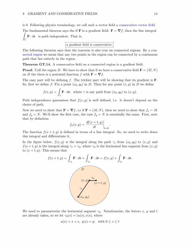
In the figure below, f(x, y) is the integral along the path γ1 from (x0, y0) to (x, y) andf(x+ t, y) is the integral along γ1 + γ2, where γ2 is the horizontal line segment from (x, y)to (x+ t, y). This means that

f(x+ t, y) =

∫

γ1

F · dr +

∫

γ2

F · dr = f(x, y) +

∫

γ2

F · dr.

(x0, y0)

(x, y)(x+ t, y)

γ1

γ2

D

We need to parameterize the horizontal segment γ2. Notationwise, the letters x, y and tare already taken, so we let γ2(s) = (u(s), v(s), where

u(s) = x+ s, y(s) = y; with 0 ≤ s ≤ t

9 POTENTIAL FUNCTIONS 15

On this segment du = ds and dy = 0. So,

f(x+ t, y) = f(x, y) +

∫ t

0M(x+ s, y) ds

The piece f(x, y) is constant as t varies, so the fundamental theorem of calculus says that

df(x+ t, y)

dt= M(x+ t, y).

Setting t = 0 we have

fx(x, y) =df(x+ t, y)

dt

∣∣∣∣t=0

= M(x, y).

This is exactly what we needed to show! We summarize in a box:

On a connected region a conservative field is a gradient field.

Example GT.15. If F is the electric field of an electric charge it is conservative.

Example GT.16. A gravitational field of a mass is conservative.

9 Potential functions

Definition. If F = ∇f is a gradient vector field then we call f a potential function for F.

Note. The usual physics terminology would be to call −f the potential function for F.

This section is devoted to answering two questions.

1. How do we know if a vector field F is a gradient vector field, i.e. if F = ∇f for somepotential function f?

2. If it exists, how do we find the potential function f?

9.1 First answers to our questions

Theorem GT.17. Suppose F = (M,N). We have the following answer to our twoquestions.

(a) If F = ∇f , then∂M

∂y=∂N

∂x, i.e. My = Nx.

(b) If My = Nx in the whole plane then F is a gradient vector field, i.e F = ∇f for somepotential function f .

(c) If F is conservative on a connected region, then F is a gradient field.

Notes. The restriction that F is defined on the whole plane is too stringent for our needs.Below, we will give what we call the Potential theorem, which only requires that F bedefined and differentiable on what is called a ‘simply connected region’.

Proof of (a). If F = (M,N) = ∇f then M = fx and N = fy. This implies,

My = fxy and Nx = fyx, i.e My = Nx. QED.

(Provided f has continuous second partials.)


The proof of (b) will be postponed until after we have proved Green’s theorem and wecan state the Potential theorem. Part (c) is just a restatement of Theorem GT.14. Theexamples below will show how to find f

Example GT.18. For which values of the constants a and b will F =(axy, x2 + by

)be a

gradient field?

answer: My = ax, Nx = 2x. To apply the theorem we need My = Nx in the entire plane.So, a = 2 and b is arbitrary.

Example GT.19. Is F =((3x2 + y), ex

)conservative?

answer: First we check if it is a gradient field: We write F = (M,N) =(3x2 + y, ex

).

Then, My = 1, Nx = ex. Since My 6= Nx, F is not a gradient field. Now, TheoremGT.17(c) says it can’t be conservative.

Example GT.20. Is(−y, x)

x2 + y2conservative?

answer: NO! The reasoning is a little trickier than in the previous example. First, it isnot hard to compute that

My =y2 − x2

(x2 + y2)2= Nx.

BUT, since the field is not defined for all (x, y), Theorem GT.17(b) does not apply. So, allwe can say at this point is that we haven’t ruled out its being conservative.

To show that it’s not conservative we will find a closed path where the line integral is not0. In fact, we will use our super-duper important example from above.

Let C = unit circle parametrized by x = cos(t), y = sin(t).

Writing everything in terms of t:

dx = − sin(t) dt, dy = cos(t) dt, M = − y

x2 + y2= − sin(t), N =

x

x2 + y2= cos(t).

Putting this in the line integral

∮

CF · dr =

∮

CM dx+N dy =

∮ 2π

0sin2(t) + cos2(t) dt =

∫ 2π

0dt = 2π

Since this is not 0, the field is not conservative.

Example GT.21. Is F =(x, y)

x2 + y2conservative?

answer: Again it is easy to check that Nx = My, BUT since F is not defined at (0, 0)Theorem GT.17(b) does not apply. HOWEVER, it turns out that

F = ∇ ln(√x2 + y2) = ∇ ln r

Since F is a gradient field, it is conservative. (Officially, we should say, F is conservative onthe region consisting of the plane minus the origin.)


9.2 Finding the potential function

We will show two methods for finding the potential functions. In general, for 18.04 themethod of integrating along a rectangular path is more relevant.

Example GT.22. Show that F =(3x2 + 6xy, 3x2 + 6y

)is conservative and find the

potential function f such that F = ∇f .

answer: We have F = (M,N), where M = 3x2 + 6xy, N = 3x2 + 6y.

First, My = 6x = Nx. Since F is defined for all (x, y) Theorem GT.17 implies F is agradient field, hence conservative.

Method 1 for finding f .

Since F is a gradient field we know

∫

CF · dr = f(Q)− f(P ) for any path from P to Q. We

make use of this by letting C be a rectangular path from the origin to an arbitrary pointQ = (x1, y1) (see figure).

x

y

C1

C2y1 Q = (x1, y1)

Rectangular path from the origin to Q.

We know

∫

C1+C2

F · dr = f(x1, y1)− f(0, 0). So

f(x1, y1) =

∫

C1+C2

F · dr + f(0, 0).

On the rectangular path shown dx = 0 on C1 and dy = 0 on C2. Therefore,∫

C1+C2

F · dr =

∫

C1

N dy +

∫

C2

M dx.

These integrals are straightforward to compute. We do each one separately.

Integral over C1:Parametrize C1: parameter = y: x = 0, y = y, y runs from 0 to y1.

Put everything we need in terms of the parameter y:

dy = dy, N = 3x2 + 6y = 6y.

Put this in the integral and compute∫

C1

N dy =

∫ y1

06y dy = 3y21.

Integral over C2 :Parameter = x: x = x, y = y1, x runs from 0 to x1.


Put everything we need in terms of the parameter x:

dx = dx, M = 3x2 + 6xy = 3x2 + 6xy1

Put this in the integral and compute (remember y1 is a constant):

∫

C2

M dx =

∫ x1

03x2 + 6xy1 dx = x31 + 3x21y1.

So,

f(x1, y1)− f(0, 0) =

∫

C1+C2

F · dr = 3y21 + x31 + 3x21y1.

Now, we are free to choose any value for f(0, 0), i.e. it is an arbitrary constant of integrationc. So, dropping the subscripts on x1 and y1, we have

f(x, y) = 3y2 + x3 + 3x2y + c.

Method 2 for finding f .

We know M = fx and N = fy. We start by integrating M with respect to x.

fx = 3x2 + 6xy ⇒ f(x, y) = x3 + 3x2y + g(y).

The function g(y) is the ‘constant of integration’ with respect to x.

Now fy = N , so differentiating our expression for f we get

fy = 3x2 + g′(y) = N = 3x2 + 6y.

Thus, g′(y) = 6y, which implies g(y) = 3y2 + c. Using this in our expression for f , we have

f(x, y) = x3 + 3x2y + g(y) = 3x2y + 3y2 + x3 + c.

(Same as method 1.)

Example GT.23. Let F =((x+ y2), (2xy + 3y2)

). Show that F is a gradient field and

find the potential function using both methods.

answer: Testing the partials we have: My = 2y = Nx, F defined on all (x, y). Thus, byTheorem GT.17, F is conservative.

Method 1: Use the path shown.

x

y

C1

C2

x1

Q = (x1, y1)

We know f(x1, y1)− f(0, 0) =∫C1+C2

F · dr =∫C1M dx+

∫C2N dy,

Parametrize C1: x = x, y = 0, x runs from 0 to x1.

In terms of the parameter x along C1: dx = dx, M = x+ y2 = x.

10 GREEN’S THEOREM 19

Integrating: ∫

C1

M dx =

∫ x1

0x dx =

x212.

Parametrize C2: x = x1, y = y, y runs from 0 to y1.

In terms of the parameter y along C2: dy = dy, N = 2x1y + 3y2.

Integrating: ∫

C2

N dy =

∫ y1

02x1y + 3y2 dy = x1y

21 + y31.

So, f(x1, y1) =

∫

C1+C2

F · dr + f(0, 0) =x212

+ x1y21 + y31 + f(0, 0).

Letting f(0, 0) = c and dropping the subscripts on x1, y1 we have

f(x, y) =x2

2+ xy2 + y3 + c.

Method 2. Since, in 18.04, we are less interested in method 2, we’ll leave this to the reader.

10 Green’s theorem

Green’s theorem is the one of the big theorems of multivariable calculus. It relates lineintegrals and area integrals. Using this relation we can often compute a seemingly difficultintegral without integration or reduce it to an easy integral. At the this section we willdescribe how it is analogous to the fundamental theorem of calculus.

10.1 Simple closed curves

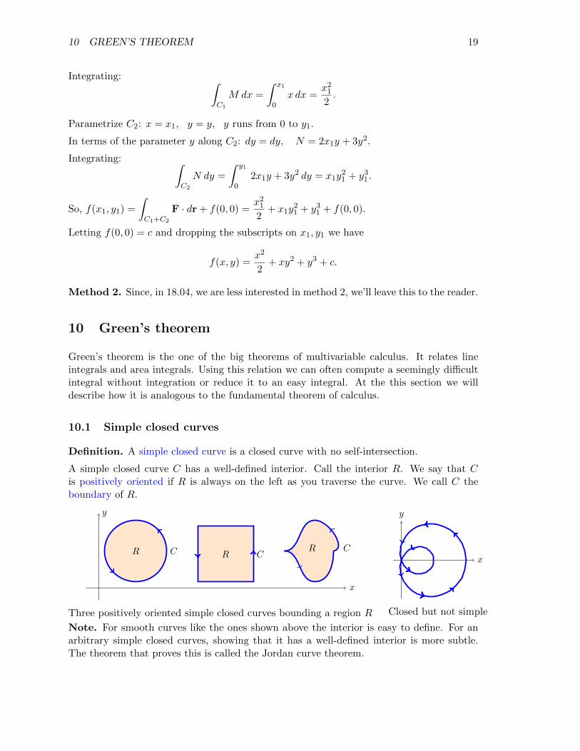
Definition. A simple closed curve is a closed curve with no self-intersection.

A simple closed curve C has a well-defined interior. Call the interior R. We say that Cis positively oriented if R is always on the left as you traverse the curve. We call C theboundary of R.

x

y

R C R CR C

Three positively oriented simple closed curves bounding a region R

x

y

Closed but not simple

Note. For smooth curves like the ones shown above the interior is easy to define. For anarbitrary simple closed curves, showing that it has a well-defined interior is more subtle.The theorem that proves this is called the Jordan curve theorem.


10.2 Green’s theorem

Theorem GT.24. Green’s theorem. Let C be a positively oriented simple closed curvewith interior region R. We assume C is piecewise smooth (a few corners are okay). If thevector field F = (M,N) is defined and differentiable on R then

∮

CM dx+N dy =

∫∫

RNx −My dA. (4)

In two dimensions we define curlF = Nx −My. So, in vector form, Green’s theorem iswritten ∮

CF · dr =

∫∫

RcurlF dA.

Example GT.25. (Using the right hand side of Equation 4 to find the left hand side.)

Use Green’s theorem to compute

I =

∮

C3x2y2 dx+ 2x2(1 + xy) dy

where C is the circle shown.

x

y

C

a

answer: The line integral is of the form on the left hand side of Green’s theorem. So, byGreen’s theorem we can convert the line integral to an area integral. In the line integralM = 3x2y2, N = 2x2(1 + xy), so Nx −My = 6x2y + 4x− 6x2y = 4x. Therefore,

I =

∮

C3x2y2 dx+ 2x2(1 + xy) dy =

∫∫

RNx −My dx dy = 4

∫∫

Rx dx dy.

We could compute this directly, but here’s a trick. We know the x center of mass is

xcm =1

A

∫∫

Rx dx dy = a.

Since area A = πa2, we have

∫∫

Rx dx dy = πa3, so I = 4πa3.

Example GT.26. (Using the left hand side of Equation 4 to find the right hand side.)

Use Green’s theorem to find the area under one arch of the cycloid.

answer: Our strategy is to use Green’s theorem to replace the area integral with a lineintegral. The figure shows one arch of the cycloid. The region is under the arch and abovethe x-axis. The boundary of the region is C = C1 + C2.


x

y

C1

C2

R

2a

πa 2πa

The trick is to use the vector field F = (−y, 0), so curlF = Nx −My = 1. With this F,Green’s theorem says

∮

CF · dr =

∮

C−y dx =

∫∫

RNx −My dA =

∫∫

RdA = area

That is, the area is equal to the line integral

∮

C−y dx. We compute the line integral as

usual:

Parametrize C1: x = x, y = 0, x runs from 0 to 2πa. So,

dx = dx, dy = 0, M = −y = 0, N (skip N because dy = 0).

Thus

∫

C1

F · dr = 0.

Parametrize C2: x = a(θ − sin(θ)), y = a(1 − cos(θ)), θ runs from 2π to 0. (Note thedirection θ runs.) So,

dx = a(1−cos(θ)) dθ, dy (skip dy because N = 0), M = −y = −a(1−cos(θ)), N = 0.

Computing the integral over C2:

∫

C2

F · dr =

∫

C2

−y dx =

∫ 0

2π−a2(1− cos(θ))2 dθ =

∫ 2π

0a2(1− cos(θ))2 dθ = 3πa2.

(The integral is easily computed by expanding the square and using the half-angle formula.)

Adding the two integrals: the area under one arch of the cycloid is 3πa2.

10.3 Other ways to compute area using line integrals

The key to the previous example was that for F = (−y, 0) we had curlF = Nx −My = 1.There are other vector fields with the property curlF = 1. For example, F = (0, x) orF = (−y/2, x/2). Using Green’s theorem we have

Area of R =

∮

C−y dx

∮

Cx dy =

1

2

∮

C−y dx+ x dy.

Here C is the positively oriented curve that bounds R.

10.4 ’Proof’ of Green’s theorem

(i) First we’ll work on the rectangle shown. Later we’ll use a lot of rectangles to approximatean arbitrary region.


x

y

a b

c

d

(ii) We’ll simplify a bit and assume N = 0. The proof when N 6= 0 is essentially the samewith a bit more writing.

First we consider the right hand side of Green’s theorem (Equation 4). By direct calculation(assuming N = 0), the right hand side is

∫∫

R−My dA =

∫ b

a

∫ d

c−∂M∂y

(x, y) dy dx.

The inner integral is the integral with respect to y of a derivative with respect to y. Thatis, we can compute it using the fundamental theorem of calculus.

∫ d

c

∂M

∂y(x, y) dy = −M(x, y)|dc = −M(x, d) +M(x, c)

Putting this into the outer integral we have shown that

∫∫

R−∂M∂y

dA =

∫ b

aM(x, c)−M(x, d) dx. (5)

Next we consider the left hand side of Equation 4. We have (remember N = 0) to compute∮

CM dx. C has four sides we parametrized each one:

bottom: x = x, y = c, x runs from a to b, dx = dx

top: x = x, y = d, x runs from b to a, dx = dx

sides: skip because dx = 0.

So,∮

CM dx =

∫

bottomM dx+

∫

topM dx (since dx = 0 along the sides)

=

∫ b

aM(x, c) dx+

∫ a

bM(x, d) dx =

∫ b

aM(x, c)−M(x, d) dx. (6)

Comparing Equations 5 and 6 we find that we have proved Green’s theorem for the rectangle.

Next we’ll use rectangles to build up an arbitrary region. We start by stacking two rectangleson top of each other.

For line integrals when adding two rectangles with a common edge the common edges aretraversed in opposite directions. So, the sum of the line integrals over the two rectanglesequals the line integral over the outside boundary.

11 ANALOGY TO THE FUNDAMENTAL THEOREM OF CALCULUS 23

=

Similarly when adding a lot of rectangles: everything cancels except the outside boundary.This extends Green’s theorem on a rectangle to Green’s theorem on a sum of rectangles.Since any region can be approximated as closely as we want by a sum of rectangles, Green’stheorem must hold on arbitrary regions. (See figure below.)

≈

Any region and boundary can be approximated as a sum of rectangles.

11 Analogy to the fundamental theorem of calculus

We saw in the proof of Green’s theorem that at one key step we had to integrate

∫∂M

∂ydy.

To do this we literally used the fundamental theorem. There is another way to view thisconnection. We will be rather informal in describing it, but it can be made formal and hasdeep and wide-ranging applications in math and science.

To set up the analogy we recall the fundamental theorem of calculus

∫ b

aF ′(x) dx = F (b)− F (a)

Here’s a picture of the domain of integration:

xa b

Notice that the left hand side of the fundamental theorem involves the integral of thederivative of F over a region (interval), and the right hand side is a sum of F itself over theboundary (endpoints) of the region.

12 SIMPLY CONNECTED REGIONS 24

Likewise, Green’s theorem says

∫∫

RcurlF dA =

∮

CF · dr.

The left hand side involves the integral of a derivative of F (i.e. curlF = Nx −My) over aregion, and the right hand side is an integral (i.e. a ‘sum’) of F itself over the boundary ofthe region. This is exactly the same language we used to describe the fundamental theoremof calculus.

12 Simply connected regions

We will need the topological notion of a simply connected region. We will stick with aninformal definition of simply connected that will be sufficient for our purposes.

(For those who are interested: We will assume that a simple closed curve has an inside andan outside. This is intuitive and is easy to show if C is a smooth curve, but turns out tosurprisingly hard if we allow C to be strange, e.g. a Koch snowflake.)

Definition: A region D in the plane is called simply connected if, for every simple closedcurve that lies entirely in D the interior of C also lies entirely in D.

Examples:

D1 D2 D3

x

y

D4

x

y

D5 = whole plane

D1-D5 are simply connected, since for any simple closed curve inside them its interior isentirely inside the region. This is sometimes phrased as each region has “no holes”.

Note. An alternative definition, which works in higher dimensions is that the region issimply connected if any curve in the region can be continuously shrunk to a point withoutleaving the region.

The regions at below are not simply connected. That is, the interior of the curve C is notentirely in the region.

C

Annulus

x

y

C

Puntured plane

13 POTENTIAL THEOREM AND CONSERVATIVE FIELDS 25

13 Potential theorem and conservative fields

As an application of Green’s theorem we can now give a more complete answer to ourquestion of how to tell if a field is conservative. The theorem does not have a standardname, so we choose to call it the Potential theorem. You should check that it is largely arestatement for simply connected regions of Theorem GT.17 above.

Theorem GT.27. (Potential theorem) Take F = (M,N) defined and differentiable on aregion D.

(a) If F = ∇f then curlF = Nx −My = 0.

(b) If D is simply connected and curlF = 0 on D, then F = ∇f for some f .

Notes.

1. We know that on a connected region, being a gradient field is equivalent to beingconservative. So we can restate the Potential theorem as: On a simply connected region, Fis conservative is equivalent to curlF = 0.

2. Recall that once we know work integral is path independent, we can compute thepotential function f by picking a base point P0 in D and letting

f(Q) =

∫

CF · dr,

where C is any path in D from P0 to Q.

Proof of (a): This was proved in Theorem GT.17.

Proof of (b): Suppose C is a simple closed curve in D. Since D is simply connected theinterior of C is also in D. Therefore, using Green’s theorem we have,

∮

CF · dr =

∫∫

RcurlF dA = 0.

x

y

D

CR

This shows that F is conservative in D. Therefore by Theorem GT.14, F is a gradient field.

Summary: Suppose the vector field F = (M,N) is defined on a simply connected regionD. Then, the following statements are equivalent.

(1)

∫ Q

PF · dr is path independent.

(2)

∮

CF · dr = 0 for any closed path C.

14 EXTENDED GREEN’S THEOREM 26

(3) F = ∇f for some f in D

(4) F is conservative in D.

If F is continuously differentiable then 1, 2, 3, 4 all imply 5:

(5) curlF = Nx −My = 0 in D

13.1 Why we need simply connected in the Potential theorem

The basic idea is that if there is a hole in D, then F might not be defined on the interior ofC. This is illustrated in the next example.

Example GT.28.(What can go wrong if D is not simply connected.) Here we will repeatthe super-duper really important Example GT.9.

Let F =(−y, x)

r2(“tangential field”).

F is defined on D = plane - (0,0) = punctured plane

x

y

C

Puntured plane

Several times now we have shown that curlF = 0. (If you’ve forgotten this, you shouldrecompute it now.) We also know that on any circle C of radius a centered at the origin∫

CF · dr = 2π.

So, the conclusion of the above theorem that curlF = 0 implies F is conservative does nothold. The problem is that D is not simply connected and, in fact, F is not defined on theentire region inside C, so we are not able to apply Green’s theorem to conclude that theline integral is 0.

14 Extended Green’s theorem

We can extend Green’s theorem to a region R which has multiple boundary curves. Thefigures below show regions bounded by 2 or more curves. You will see that this gives usaway to work around singularities in the field F.

14.1 Regions with multiple boundary curves

Consider the following three regions.


C1

C2

RA

C3

C4 C5 C6

RB

C7

C8

RC

The region on the left, RA is bounded by C1 and C2. We say that the boundary is C1 +C2.Note that the way it is drawn, the region is always to the left as you traverse either boundarycurve.

The region on the right, RC is bounded by C7 and C8. We say that the boundary is C7−C8.The reason for the minus sign is that the boundary curves should be oriented so that theregion is to your left as you traverse the curve. As shown, the region RC is to the right ofC8, but to the left of −C8.

Likewise, in the middle figure, RB has boundary C3 +C4 +C5 +C6. You should check thatour signs are consistent with the orientation of the curves.

14.2 Extended Green’s theorem

Theorem GT.29. Extended Green’s theorem. Suppose RA is the region in the left-handfigure above then, for any vector field F differentiable in all of RA we have

∮

C1+C2

F · dr =

∫∫

RA

curlF dx dy.

Likewise for more than two curves: If RB has boundary C3 + C4 + C5 + C6 and F isdifferentiable on all of RB then

∮

C3+C4+C5+C6

F · dr =

∫∫

RB

curlF dx dy.

Proof. We will prove the formula for RA. The case of more than two curves is essentiallythe same. The key is to make the ‘cut’ shown in the figure below, so that the resultingcurve is simple.

C1

C2

C3−C3

RA

In the figure the curve C1 + C3 + C2 − C3 surrounds the region RA. (You have to imaginethat the cut is infinitesimally wide so C3 and −C3 are right on top of each other.)

Now the original Green’s theorem applies:∮

C1+C3+C2−C3

F · dr =

∫∫

RcurlF dx dy


Since the contributions of C3 and −C3 will cancel, we have proved the extended form ofGreen’s theorem. ∮

C1+C2

F · dr =

∫∫

RcurlF dx dy. QED

Example GT.30. Again, let F be the tangential field F =(−y, x)

r2. What values can

∮

CF · dr take for C a simple closed positively oriented curve that doesn’t go through the

origin?

answer: We have two cases (i) C1 does not go around 0; (ii) C2 goes around 0

C1R1

C2

R2 x

y

Case (i) We know F is defined and curlF = 0 in the entire region inside C1, so Green’stheorem implies ∮

C1

F · dr =

∫∫

RcurlF dx dy = 0.

Case (ii) We can’t apply Green’s theorem directly because F is not defined everywhereinside C2. Instead, we use the following trick. Let C3 be a circle centered on the origin andsmall enough that is entirely inside C2.

x

y

C2C3R2

The region R2 has boundary C2 − C3 and F is defined and differentiable in R2. We knowthat curlF = 0 in R2, so extended Green’s theorem implies

∫

C2−C3

F · dr =

∫∫

R2

curlF dx dy = 0.

So

∫

C2

F · dr =

∫

C3

F · dr.

Since C3 is a circle centered on the origin we can compute the line integral directly –we’ve

15 ONE MORE EXAMPLE 29

done this many times already. ∮

C3

F · dr = 2π.

Therefore, for a simple closed curve C and F as given, the line integral

∮

CF · dr is either

2π or 0, depending on whether C surrounds the origin or not.

Answer to the question: The only possible values are 0 and 2π.

Example GT.31. Use the same F as in the previous example. What values can the lineintegral take if C is not simple.

answer: If C is not simple we can break it into a sum of simple curves.

x

y

C1

C2

In the figure, we can think of the entire curve as C1 + C2. Since each of these curvessurrounds the origin we have

∫

C1+C2

F · dr =

∫

C1

F · dr +

∫

C2

F · dr = 2π + 2π = 4π.

In general,

∮

CF · dr = 2πn, where n is the number of times C goes around (0,0) in a

counterclockwise direction.

Aside for those who are interested: The integer n is called the winding number of Caround 0. The number n also equals the number of times C crosses the positive x-axis,counting +1 if it crosses from below to above and −1 if it crosses from above to below.

15 One more example

Example GT.32. Let F = rn (x, y) .

For n ≥ 0, F is defined on the entire plane. For n < 0, F is defined on the xy-plane minusthe origin (the punctured plane).

Use extended Green’s theorem to show that F is conservative on the punctured plane forall integers n. Then, find a potential function.

answer: We start by computing the curl:

M = rnx ⇒ My = nrn−2xy

N = rny ⇒ Nx = nrn−2xy


So, curlF = Nx −My = 0.

To show that F is conservative in the punctured plane, we will show that

∫

CF · dr = 0 for

all simple closed curves C that don’t go through the origin.

If C is a simple closed curve not around 0 then F is differentiable on the entire region inside

C and Green’s theorem implies

∫

CF · dr =

∫∫

RcurlF dx dy = 0.

If C is a simple closed curve that surrounds 0, then we can use the extended form of Green’stheorem as in Example GT.30

x

y

CC2R

We put a small circle C2 centered at the origin and inside C.

Since F is radial, it is orthogonal to C2. So, on C2, F · dr = 0, which implies

∮

C2

F · dr = 0.

Now, on the region R with boundary C − C2 we can apply the extended Green’s theorem

∮

C−C2

F · dr =

∫∫

RcurlF dx dy = 0.

Thus,

∮

CF · dr =

∮

C2

F · dr, which, as we saw, equals 0.

Thus

∮

CF · dr = 0 for all closed loops, which implies F is conservative. QED

To find the potential function we use method 1 over the curve C = C1 + C2 shown.

x

y

C1

C2(x1, y1)

(1, 1)

The following calculation works for n 6= −2. For n = −2 everything is the same except weget natural logs instead of powers.

Parametrize C1 using y: x = 0, y = y; y from 1 to y1. So,


dx = 0, dy = dy, skip M , since dx = 0, N = rny = y(1 + y2)n/2. So,

∫

C1

F · dr =

∫

C1

M dx+N dy =

∫ y1

1y(1 + y2)n/2 dy

=(1 + y2)(n+2)/2

n+ 2

∣∣∣∣∣

y1

1

(u-substitution: u = 1 + y2)

=(1 + y21)(n+2)/2

n+ 2− 2(n+2)/2

n+ 2.

Parametrize C2 using x: x = x, y = y1; x from 1 to x1. So,

dx = dx, dy = 0, M = rnx = x(x2 + y21)n/2 skip, N since dy = 0. So,

∫

C2

F · dr =

∫

C2

M dx+N dy =

∫ x1

1x(x2 + y21)n/2 dx

=(x2 + y21)(n+2)/2

n+ 2

∣∣∣∣∣

x1

1

(u-substitution: u = x2 + y21)

=(x21 + y21)(n+2)/2

n+ 2− (1 + y21)(n+2)/2

n+ 2.

Adding these we get f(x1, y1)− f(1, 1) =(x21 + y21)(n+2)/2 − 2(n+2)/2

n+ 2. So,

f(x, y) =rn+2

n+ 2+ c. (If n = −2 we get f(x, y) = ln r + C.)

(Note, we ignored the fact that if (x1, y1) is on the negative x-axis we shoud have used adifferent path that doesn’t go through the origin. This isn’t really an issue because we knowthere is a potential function. Because our function f is known to be a potential functioneverywhere except the negative x-axis, by continuity it also works on the negative x-axis.)

line integrals and green’s theorem jeremy orlojorloff/18.04/notes/greenstheorem.pdf · line...

Documents