Canadian Institute of Steel Construction, 2012

LIMIT STATES DESIGN IN STRUCTURAL STEEL

G.L. Kulak and G.Y. Grondin

9th Edition, 1st Printing 2010

REVISIONS LIST NO. 1 - JANUARY 2012

Revisions and updates incorporated into the 9th Edition, 2nd Printing (2011) of Limit States Design in Structural Steel are highlighted in red boxes on the following pages. Minor editorial corrections are not shown.

53

In this example, fracture through Section 1–1, or an equivalent section in member B, is the only possible net section fracture location. An example in which the area of a staggered section must be calculated will follow. Carrying this illustration to its conclusion, the tensile capacity of member A now can be determined. For G40.21 300W steel, yF = 300 MPa and uF = 450 MPa. Calculation of the tensile resistance, rT , using Equations 3.1 and 3.2 gives = φ = × × = ×=

2 2 3r g yT A F 0.90 5000 mm 300 N / mm 1350 10 N1350 kN or = φr u n uT A F = × ×2 20.75 3700 mm 450 N / mm = × =31249 10 N 1249 kN (Governs) The value of the factored resistance, rT = 1249 kN, can now be compared with the effect of the factored loads in the member under consideration. It should also be noted that the yield point of this steel was taken to be 300 MPa. In fact, the yield strength of plates is a function of thickness. Table 4 of Appendix A shows that the yield strength for Grade 300W steel is 300 MPa for plate thicknesses up to 65 mm. Since the plate thickness used in this example is 25 mm, the assumption used here is valid. This example will not be used to investigate the possible block shear failure. That will be illustrated later.

( )[ ]= − + × = 2neA 200 22 4 mm 25 mm 4350 mm Referring to the preceding example, a cross-section of 3700 2mm will be loaded to its maximum permissible capacity under a factored load of 1274 kN. However, a cross section of 5000 2mm was provided for most of the length of the member. This means that 35% more cross-sectional area than is necessary is being used for a greater part of the member. While the ideal of 100% efficiency is not attainable when mechanical fasteners are used, the designer might look for a more favourable fastener pattern. One alternative is shown in Figure 3.9. Two cases will be examined, a tearing of the plate directly across Section 1–1 or through in a zig-zag fashion as in Section 2–2. Referring again to Figure 3.9 and assuming values of w = 200 mm, s = 80 mm, and g = 115 mm, and the use of 22 mm diameter bolts in punched holes, the net areas are: Section 1–1 ( )[ ]= − + × = 2neA 200 22 4 mm 25 mm 4350 mm Section 2–2 ( )⎡ ⎤

= − × + + × =⎢ ⎥×⎣ ⎦

2 2ne 80A 200 2 22 4 mm 25 mm 4048 mm4 115 Section 2–2 governs, and the net area ( nA ) to be used in Equation 3.2 is 4048 2mm .

54

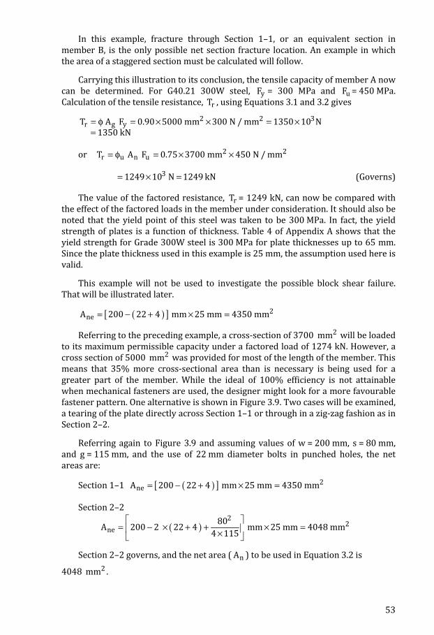
The efficiency of this connection is now =4048 5000 81% , a considerable improvement over that obtained with the previous fastener arrangement. The improvement does come at the expense of having to make a longer joint, however. 1 2

1,2

w

Transversespacing orgauge, g

Stagger or pitch, s Figure 3.9 – Tension Member – Staggered Fasteners The capacity of this member can now be established. Since the plate thickness involved is less than 65 mm, the yield strength of the Grade 300W material is 300 MPa. Checking Equations 3.1 and 3.2 gives, respectively,

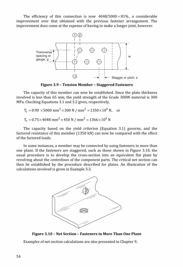
= × × = ×2 2 3rT 0.90 5000 mm 300 N / mm 1350 10 N, or = × × = ×2 2 3rT 0.75 4048 mm 450 N / mm 1366 10 N The capacity based on the yield criterion (Equation 3.1) governs, and the factored resistance of this member (1350 kN) can now be compared with the effect of the factored loads. In some instances, a member may be connected by using fasteners in more than one plane. If the fasteners are staggered, such as those shown in Figure 3.10, the usual procedure is to develop the cross-section into an equivalent flat plate by revolving about the centrelines of the component parts. The critical net section can then be established by the procedure described for plates. An illustration of the calculations involved is given in Example 3.3.

Figure 3.10 – Net Section – Fasteners in More Than One Plane Examples of net section calculations are also presented in Chapter 9.

55

3.7 Design Examples The preceding sections have set out the basis of design of tension members. As has been noted, one of the main criteria affecting the design will be the connection details. If the end connection is to be made using welds, there generally is no resulting reduction in cross-section and, if there is no shear lag reduction to be made, the design of the member can proceed directly. When bolts are to be used, however, the design of the member is influenced by the amount of material removed in making the connection. In turn, the design of the connection itself cannot proceed without a knowledge of the shape to be used. As with most design problems, the engineer must work in a trial and error fashion until all relevant aspects have been satisfied. Example 3.1

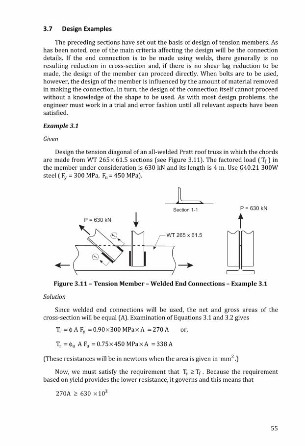
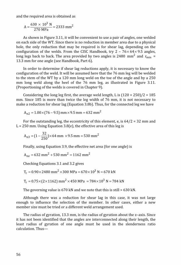
Given Design the tension diagonal of an all-welded Pratt roof truss in which the chords are made from WT 265× 61.5 sections (see Figure 3.11). The factored load ( fT ) in the member under consideration is 630 kN and its length is 4 m. Use G40.21 300W steel ( yF = 300 MPa, uF = 450 MPa).

1

1

P = 630 kN

WT 265 x 61.5

P = 630 kNSection 1-1

Figure 3.11 – Tension Member – Welded End Connections – Example 3.1

Solution Since welded end connections will be used, the net and gross areas of the cross-section will be equal (A). Examination of Equations 3.1 and 3.2 gives = φ = × × =r yT A F 0.90 300 MPa A 270 A or, = φ = × × =r u uT A F 0.75 450 MPa A 338 A (These resistances will be in newtons when the area is given in 2mm .) Now, we must satisfy the requirement that ≥r fT T . Because the requirement based on yield provides the lower resistance, it governs and this means that

≥ × 3270A 630 10

56

and the required area is obtained as ×= =

3 2630 10 NA 2333 mm270 MPa As shown in Figure 3.11, it will be convenient to use a pair of angles, one welded on each side of the WT. Since there is no reduction in member area due to a physical hole, the only reduction that may be required is for shear lag, depending on the configuration of the welds. From the CISC Handbook, try 2 – 76× 64× 9.5 angles, long legs back to back. The area provided by two angles is 2480 2mm and minr = 13.3 mm for one angle (see Handbook, Part 6). In order to determine if shear lag reductions apply, it is necessary to know the configuration of the weld. It will be assumed here that the 76 mm leg will be welded to the stem of the WT by a 120 mm long weld on the toe of the angle and by a 250 mm long weld along the heel of the 76 mm leg, as illustrated in Figure 3.11. (Proportioning of the welds is covered in Chapter 9). Considering the long leg first, the average weld length, L is (120 + 250)/2 = 185 mm. Since 185 is more than twice the leg width of 76 mm, it is not necessary to make a reduction for shear lag (Equation 3.8b). Thus, for the connected leg we have = × − × = 2n2A 1.00 (76 9.5) mm 9.5 mm 632 mm For the outstanding leg, the eccentricity of this element, e, is 64/2 = 32 mm and L = 250 mm. Using Equation 3.8(e), the effective area of this leg is = − × × = 2n3 32A (1 ) 64 mm 9.5 mm 530 mm250 Finally, using Equation 3.9, the effective net area (for one angle) is = + =2 2 2neA 632 mm 530 mm 1162 mm Checking Equations 3.1 and 3.2 gives

= × × = × =2 3rT 0.90 2480 mm 300 MPa 670 10 N 670 kN = × × × = × =2 3rT 0.75 (2 1162) mm 450 MPa 784 10 N 784 kN The governing value is 670 kN and we note that this is still > 630 kN. Although there was a reduction for shear lag in this case, it was not large enough to influence the selection of the member. In other cases, either a new member size must be tried or a different weld arrangement used. The radius of gyration, 13.3 mm, is the radius of gyration about the z–axis. Since it has not been identified that the angles are interconnected along their length, the least radius of gyration of one angle must be used in the slenderness ratio calculation. Thus—

58

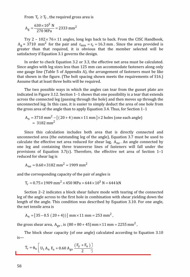
From ≥r fT T , the required gross area is ×= =

3 2g 630 10 NA 2333 mm270 MPa Try 2 – 102 × 76× 11 angles, long legs back to back. From the CISC Handbook, gA = 3710 2mm for the pair and = =min zr r 16.3 mm . Since the area provided is greater than that required, it is obvious that the member selected will be satisfactory if Equation 3.1 governs the design. In order to check Equation 3.2 or 3.3, the effective net area must be calculated. Since angles with leg sizes less than 125 mm can accommodate fasteners along only one gauge line (Table 5 of Appendix A), the arrangement of fasteners must be like that shown in the figure. (The bolt spacing shown meets the requirements of S16.) Assume that at least three bolts will be required. The two possible ways in which the angles can tear from the gusset plate are indicated in Figure 3.12. Section 1–1 shows that one possibility is a tear that extends across the connected leg (passing through the hole) and then moves up through the unconnected leg. In this case, it is easier to simply deduct the area of one hole from the gross area of the angle than to apply Equation 3.4. Thus, for Section 1–1 ( )[ ]= − + × ×

=

2n 2A 3710 mm 20 4 mm 11 mm 2 holes (one each angle) 3182 mm Since this calculation includes both area that is directly connected and unconnected area (the outstanding leg of the angle), Equation 3.7 must be used to calculate the effective net area reduced for shear lag, neA . An angle connected by one leg and containing three transverse lines of fasteners will fall under the provisions of Equation 3.7(c). Therefore, the effective net area of Section 1–1 reduced for shear lag is

= × =2 2neA 0.60 3182 mm 1909 mm and the corresponding capacity of the pair of angles is = × × = × =2 3rT 0.75 1909 mm 450 MPa 644 10 N 644 kN Section 2–2 indicates a block shear failure mode with tearing of the connected leg of the angle across to the first hole in combination with shear yielding down the length of the angle. This condition was described by Equation 3.10. For one angle, the net tensile area is

( )[ ]= − + × = 2nA 35 0.5 20 4) mm 11 mm 253 mm , the gross shear area, gvA , is + + × = 2(80 80 45) mm 11 mm 2255 mm , The block shear capacity (of one angle) calculated according to Equation 3.10 is— ( )+⎡ ⎤= φ +⎢ ⎥⎣ ⎦

y ur u t n u gv F FT U A F 0.60 A 2

59

The value of =tU 0.6 is obtained from Table 3.1.

( )+⎡ ⎤= × =× × + × ×⎢ ⎥⎣ ⎦r 300 450T 0.75 432 kN / angle0.6 253 450 0.6 2255 2

For two angles, the block shear capacity is 864 kN, which is greater than the applied member force. Note that no adjustment for shear lag is necessary for the block shear failure mode since the failure plane is entirely in the connected leg. Since the capacity calculated for tensile fracture along (Section 1–1) was only 657 kN, the governing factored resistance is the latter, i.e., 657 kN. Recall that the member was selected on the basis of Equation 3.1, using the factored load of 630 kN. Obviously, Equation 3.1 is satisfied. Since the calculated factored resistance of 657 kN is larger than the factored load of 630 kN, the selected member is satisfactory. Finally, checking the slenderness ratio = = <L 4000 mmmax 245 300r 16.3 mm (Satisfactory) Use 2 – 102× 76 × 11 angles, long legs back-to-back, as shown. (If the number of bolts finally selected is different than the three assumed, then the calculations must be reviewed.)

Example 3.3

Given The lower chord of a large truss consists of two C310× 45 sections tied across the flanges with lacing bars. The critical section of the chord occurs just outside a panel point, where it is necessary to splice the member. As shown in Figure 3.13, both web and flange splice plates are provided to transfer the forces from one side of the member to the other. Determine the factored tensile resistance of the channels if the fasteners are 22 mm diameter and G40.21 350A steel is used throughout. (Use Tables 3 and 4 of Appendix A to establish that yF = 350 MPa, uF = 480 MPa.) Solution Using the CISC Handbook, the area of 2–C310 × 45 is

= × = 2gA 2 5690 11 380 mm and the corresponding capacity is (Equation 3.1) = × × = × =2 3rT 0.90 11 380 mm 350 MPa 3585 10 N 3585 kN

76

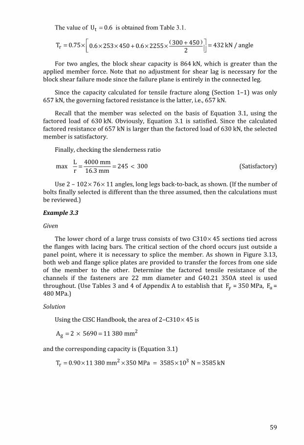
when a column buckles in the inelastic range, the initial motion is accompanied by an increase in load [4.4]. Thus, the strain distribution is actually that shown in Figure 4.9(b), with all elements of the cross-section subjected to an increase in compressive strain.

e e et = r a+ey

sy

e

s

A

Figure 4.8 – Strain Reversal in Yielded Zone

(a) (b) Figure 4.9 – Strains Induced by Buckling The load vs. deformation curve for the initially straight column is shown in Figure 4.10, where the applied stress is plotted against the midspan deformation. As the member continues to deform in its buckled shape, the load increases to its maximum value and then drops off. During this process the cross-section continues to yield. The maximum stress is not much greater than the stress at the instant of buckling.

150

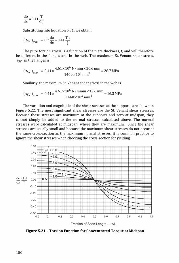
φ =d T0.41dx G J Substituting into Equation 5.31, we obtain ( ) φτ = =SV max d T tG t 0.41dx J The pure torsion stress is a function of the plate thickness, t, and will therefore be different in the flanges and in the web. The maximum St. Venant shear stress,

τSV , in the flanges is ( ) × ⋅ ×τ = × =

×

6SV max 3 44.61 10 N mm 20.6 mm0.41 26.7 MPa1460 10 mm Similarly, the maximum St. Venant shear stress in the web is ( ) × ⋅ ×τ = × =

×

6SV max 3 44.61 10 N mmm 12.6 mm0.41 16.3 MPa1460 10 mm The variation and magnitude of the shear stresses at the supports are shown in Figure 5.22. The most significant shear stresses are the St. Venant shear stresses. Because these stresses are maximum at the supports and zero at midspan, they cannot simply be added to the normal stresses calculated above. The normal stresses were calculated at midspan, where they are maximum. Since the shear stresses are usually small and because the maximum shear stresses do not occur at the same cross-section as the maximum normal stresses, it is common practice to ignore the shear stresses when checking the cross-section for yielding.

-0.50

-0.40

-0.30

-0.20

-0.10

0.00

0.10

0.20

0.30

0.40

0.50

0.0 0.1 0.2 0.3 0.4 0.5 0.6 0.7 0.8 0.9 1.0

d

dx

f G J

T

Fraction of Span Length — z/L

mL = 6.0

4.0

3.0

2.0

1.51.0

0.5

Figure 5.21 – Torsion Function for Concentrated Torque at Midspan

324

Example 9.5

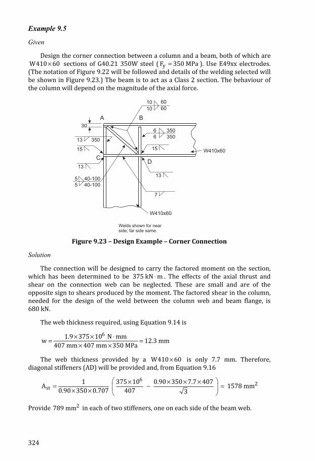
Given Design the corner connection between a column and a beam, both of which are W410 60× sections of G40.21 350W steel ( yF 350 MPa= ). Use E49xx electrodes. (The notation of Figure 9.22 will be followed and details of the welding selected will be shown in Figure 9.23.) The beam is to act as a Class 2 section. The behaviour of the column will depend on the magnitude of the axial force. A B

DC

6

5

350

40-100

6

5

10

350

60

15

10 60

13

7

W410x60

W410x60

40-100

13

15

13 350

30

Welds shown for nearside; far side same.

Figure 9.23 – Design Example – Corner Connection

Solution The connection will be designed to carry the factored moment on the section, which has been determined to be 375 kN m⋅ . The effects of the axial thrust and shear on the connection web can be neglected. These are small and are of the opposite sign to shears produced by the moment. The factored shear in the column, needed for the design of the weld between the column web and beam flange, is 680 kN. The web thickness required, using Equation 9.14 is 61.9 375 10 N mmw 12.3 mm407 mm 407 mm 350 MPa× × ⋅= =× ×

The web thickness provided by a W410 60× is only 7.7 mm. Therefore, diagonal stiffeners (AD) will be provided and, from Equation 9.16 6 2st 1 375 10 0.90 350 7.7 407A 1578 mm0.90 350 0.707 407 3⎛ ⎞× × × ×= − =⎜ ⎟× × ⎝ ⎠

Provide 2789 mm in each of two stiffeners, one on each side of the beam web.

327

2 3F 800 mm 350 MPa 280 10 N 280 kN= × = × = Length available for welding along the 80 mm wide stiffener plate is 80 20 60 mm.− = (The 20 mm accounts for the flange-to-web fillet at this location; see CISC Handbook.) Thus, at the end of one stiffener, the length available for welding is 2 60 120 mm.× = Leg size required 280 kN 15.0 mm0.156 kN/mm 120 mm= =×

This is a large fillet weld and it has to be placed into a confined space. The advantage provided by Equation 9.12b for a weld transverse to the direction of load will be invoked. For 90θ = , the increase is a factor of 1.5. Thus, the strength used in the calculation above can be increased from 0.156 kN/mm to 0.234 kN/mm . Noting that a matching electrode is used (E49XX electrode with 350W base metal), the strength of the base metal need not be considered. Recalculation of the leg size required gives 15.0 × 0.156/0.234 = 10.0 mm. Use 10 mm. Finally, transferring the 280 kN force from either end of stiffener A–D into the beam web can be done by means of a fillet weld along its length of approximately 490 mm. Thus, the length available for welding along the sides of a single stiffener at A–D is 2 490 980 mm.× = Using a continuous weld of even the smallest permissible size, 5 mm, results in a great deal more capacity than required. Therefore, an intermittent fillet weld of 5 mm leg size will be tried, using the minimum permissible weld length of 40 mm. (CSA W59 should be consulted for minimum fillet weld lengths.) A centre-to-centre spacing of 100 mm will meet the requirements of S16 Clause 19.1.3(b) and will provide a resistance of

r 0.156 kN 5 mm 40 mmV 0.312 kN / mm100 mm× ×= = The load to be transferred is 280 kNV 0.286 kN/mm980 mm= = (Satisfactory) Use an intermittent fillet weld arrangement as shown in Figure 9.23. The only other type of connection required to carry all three force components that will be discussed is the interior type connection shown in Figure 9.24. An exaggerated view of the deformed connection (Figure 9.25) shows the two possible failure modes; (a) failure of the column web as the beam flange delivers its compressive load, (b) rupture of the groove weld in the stiff region at the beam tension flange. On the compression side, it will be assumed that the force from the beam flange can be treated as a concentrated load. The design rule for this case was described in Section 5.12. The total factored force from the flange must be less than or equal to the factored web resistance at this point (Equation 5.28a). This can be expressed as

355

(a) (b)

(c)

Girt

Cladding

Innerflange

Sag rod

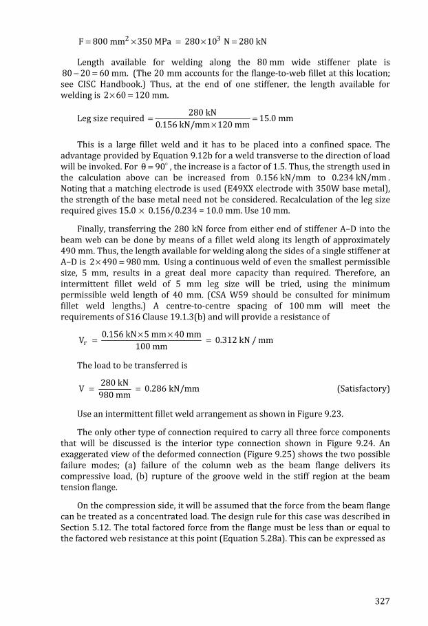
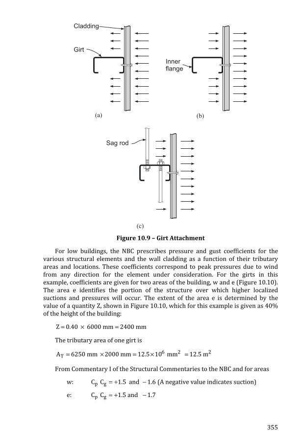
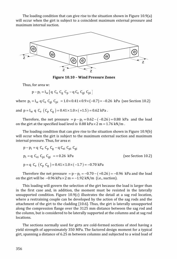
Figure 10.9 – Girt Attachment For low buildings, the NBC prescribes pressure and gust coefficients for the various structural elements and the wall cladding as a function of their tributary areas and locations. These coefficients correspond to peak pressures due to wind from any direction for the element under consideration. For the girts in this example, coefficients are given for two areas of the building, w and e (Figure 10.10). The area e identifies the portion of the structure over which higher localized suctions and pressures will occur. The extent of the area e is determined by the value of a quantity Z, shown in Figure 10.10, which for this example is given as 40% of the height of the building: Z 0.40 6000 mm 2400 mm= × = The tributary area of one girt is 6 2 2TA 6250 mm 2000 mm 12.5 10 mm 12.5 m= × = × = From Commentary I of the Structural Commentaries to the NBC and for areas w: = + −p gC C 1.5 and 1.6 (A negative value indicates suction) e: = + −p gC C 1.5 and 1.7

356

The loading condition that can give rise to the situation shown in Figure 10.9(a) will occur when the girt is subject to a coincident maximum external pressure and maximum internal suction.

z

z

z

z

e

we

e

ew

Figure 10.10 – Wind Pressure Zones Thus, for area w: [ ]i w e g p e gi pip p I q C C C q C C C− = − where i w e gi pip I q C C C 1.0 0.41 0.9 ( 0.7) 0.26 kPa= = × × × − = − (see Section 10.2) and ( ) ( )= = × × + =w e p gp I q C C C 0.41 1.0 1.5 0.62 kPa . Therefore, the net pressure ( )= − = − − =ip p 0.62 0.26 0.88 kPa and the load on the girt at the specified load level is × =0.88 kPa 2 m 1.76 kN/m . The loading condition that can give rise to the situation shown in Figure 10.9(b) will occur when the girt is subject to the maximum external suction and maximum internal pressure. Thus, for area e: i e p g ei pi gip p q C C C q C C C− = −

i ei pi gip q C C C 0.26 kPa= = + (see Section 10.2) ( ) ( )= = × × − = −e p gp q C C C 0.41 1.0 1.7 0.70 kPa Therefore the net pressure ( )= − = − − + = −ip p 0.70 0.26 0.96 kPa and the load on the girt will be − × = −0.96 kPa 2 m 1.92 kN/m (i.e., suction). This loading will govern the selection of the girt because the load is larger than in the first case and, in addition, the moment must be resisted in the laterally unsupported condition. Figure 10.9(c) illustrates the detail at a sag rod location, where a restraining couple can be developed by the action of the sag rods and the attachment of the girt to the cladding [10.6]. Thus, the girt is laterally unsupported along the compression flange over the 3125 mm distance between the sag rod and the column, but is considered to be laterally supported at the columns and at sag rod locations. The sections normally used for girts are cold-formed sections of steel having a yield strength of approximately 350 MPa. The factored design moment for a typical girt, spanning a distance of 6.25 m between columns and subjected to a wind load of

357

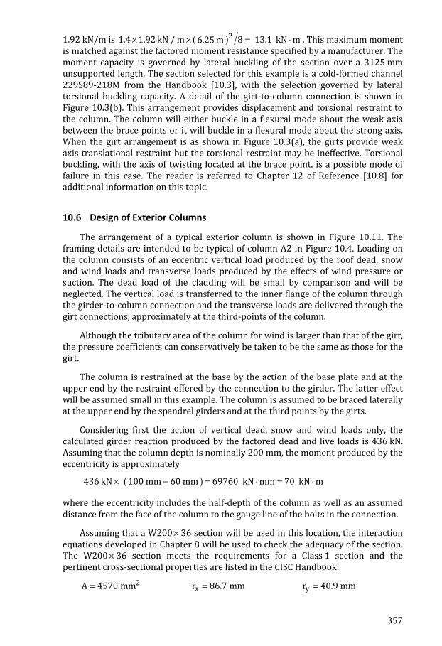
1.92 kN/m is ( )× × =21.4 1.92 kN / m 86.25 m 13.1 kN m⋅ . This maximum moment is matched against the factored moment resistance specified by a manufacturer. The moment capacity is governed by lateral buckling of the section over a 3125 mm unsupported length. The section selected for this example is a cold-formed channel 229S89-218M from the Handbook [10.3], with the selection governed by lateral torsional buckling capacity. A detail of the girt-to-column connection is shown in Figure 10.3(b). This arrangement provides displacement and torsional restraint to the column. The column will either buckle in a flexural mode about the weak axis between the brace points or it will buckle in a flexural mode about the strong axis. When the girt arrangement is as shown in Figure 10.3(a), the girts provide weak axis translational restraint but the torsional restraint may be ineffective. Torsional buckling, with the axis of twisting located at the brace point, is a possible mode of failure in this case. The reader is referred to Chapter 12 of Reference [10.8] for additional information on this topic. 10.6 Design of Exterior Columns The arrangement of a typical exterior column is shown in Figure 10.11. The framing details are intended to be typical of column A2 in Figure 10.4. Loading on the column consists of an eccentric vertical load produced by the roof dead, snow and wind loads and transverse loads produced by the effects of wind pressure or suction. The dead load of the cladding will be small by comparison and will be neglected. The vertical load is transferred to the inner flange of the column through the girder-to-column connection and the transverse loads are delivered through the girt connections, approximately at the third-points of the column. Although the tributary area of the column for wind is larger than that of the girt, the pressure coefficients can conservatively be taken to be the same as those for the girt. The column is restrained at the base by the action of the base plate and at the upper end by the restraint offered by the connection to the girder. The latter effect will be assumed small in this example. The column is assumed to be braced laterally at the upper end by the spandrel girders and at the third points by the girts. Considering first the action of vertical dead, snow and wind loads only, the calculated girder reaction produced by the factored dead and live loads is 436 kN. Assuming that the column depth is nominally 200 mm, the moment produced by the eccentricity is approximately

( ) 436 kN 100 mm 60 mm 69760 kN mm 70 kN m× + = ⋅ = ⋅ where the eccentricity includes the half-depth of the column as well as an assumed distance from the face of the column to the gauge line of the bolts in the connection. Assuming that a W200× 36 section will be used in this location, the interaction equations developed in Chapter 8 will be used to check the adequacy of the section. The W200× 36 section meets the requirements for a Class 1 section and the pertinent cross-sectional properties are listed in the CISC Handbook: 2A 4570 mm= xr 86.7 mm= yr 40.9 mm=

359

436 kN

11.7 kN

70 kN.m259 kN

259 kN

24.0 kN

10.4 kN

41.0 kN.m

17.2 kN

17.2 kN

41.0 kN.m

61.8 kN.m

48.2 kN.m

70 kN.m

11.7 kN

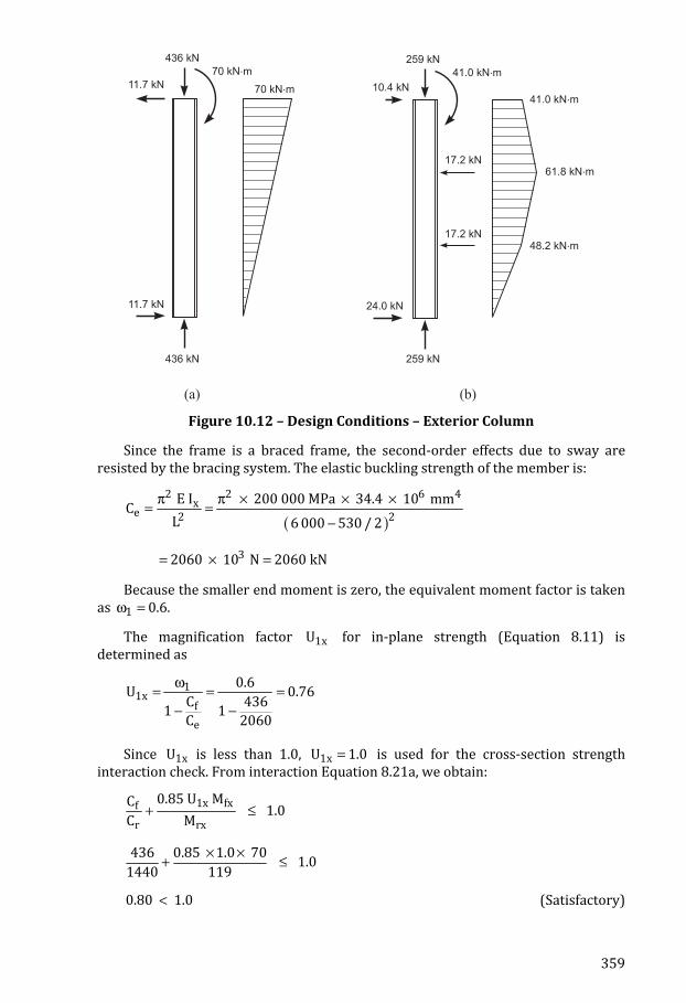
(a) (b)

436 kN Figure 10.12 – Design Conditions – Exterior Column Since the frame is a braced frame, the second-order effects due to sway are resisted by the bracing system. The elastic buckling strength of the member is:

( )

2 2 6 4xe 2 2 E I 200 000 MPa 34.4 10 mmC L 6 000 530 / 2π π × × ×= =−

32060 10 N 2060 kN= × = Because the smaller end moment is zero, the equivalent moment factor is taken as 1 0.6.ω = The magnification factor 1xU for in-plane strength (Equation 8.11) is determined as 11x fe

0.6U 0.76C 4361 1C 2060ω= = =− −

Since 1xU is less than 1.0, =1xU 1.0 is used for the cross-section strength interaction check. From interaction Equation 8.21a, we obtain: 1x fxfr rx0.85 U MC 1.0C M+ ≤

× ×+ ≤436 0.85 1.0 70 1.01440 119 <0.80 1.0 (Satisfactory)

360

For the in-plane strength check, the effective length factor K for strong axis bending is taken as 1.0 and the strong axis slenderness ratio is: ( )x 1.00 6000 530 2KL 66.1r 86.7× −⎛ ⎞ = =⎜ ⎟

⎝ ⎠

where the length of the column has been taken from the base plate to the mid height of the girder. The non-dimensional slenderness factor is calculated from Equation 4.20 as: y2 2FKL 350 MPa 66.1 0.88r E 200 000 MPaλ = = =

π π ×

The overall in-plane strength is checked using the interaction expression Equation 8.21a, where rC is taken as rxC . Therefore, λ will be based on ( )xKL r 66.1= and rxC is given by Equation 4.21.

rC ( ) 1 n2ny A F 1 −= φ + λ

( )( ) 1 1.342 1.3420.90 4570 mm 350 MPa 1 0.88 −×= × × + 3965 10 N 965 kN= × = rxM is still taken as 119 kN m.⋅ Therefore, checking the overall (in-plane) strength interaction expression, Equation 8.21a:

f 1x fxrx rxC 0.85 U M 1.0C M+ ≤

436 0.85 0.76 70 0.83 1.0965 119× ×+ = < (Satisfactory) For lateral-torsional buckling, the interaction expression is checked again using Equation 8.21a. In this case 1xU 1.0≥ ; rC is based on ( )yKL r and rxM is based on Equation 5.23. However, rxM based on Equation 5.23 still yields a value of 119 kN m⋅ , a reflection that the column is braced at the third points by the girts. Therefore, Equation 8.21a becomes f 1x fxry rxC 0.85 U M 1.0C M+ ≤

For weak axis buckling, the girts, together with the action of the cladding, effectively divide the column into three segments and prevent out-of-plane movement at these points. Thus, the weak axis slenderness ratio is: ( )y 1.00 6000/3KL 48.9r 40.9×⎛ ⎞ = =⎜ ⎟

⎝ ⎠

361

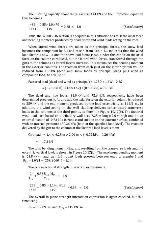
The buckling capacity about the y- axis is 1144 kN and the interaction equation thus becomes: × ×+ = ≤436 0.85 1.0 70 0.88 1.01144 119 (Satisfactory) Thus, the W200 × 36 section is adequate in this situation to resist the axial force and bending moments produced by dead, snow and wind loads acting on the roof. When lateral wind forces are taken as the principal forces, the snow load becomes the companion load. Load case 4 from Table 1.3 indicates that the wind load factor is now 1.4 and the snow load factor is 0.5. Under this condition the axial force on the column is reduced, but the lateral wind forces, transferred through the girts to the columns as lateral forces, increase. This maximizes the bending moment in the exterior columns. The reaction from each joist on the girder system will be reduced from 153 kN (dead and snow loads as principal loads plus wind as companion load) to a value of: Factored load (dead and wind as principal) = 1.25D + 1.4W + 0.5S (1.25 31.0) (1.4 12.2) (0.5 72.6) 92.1 kN= × + × + × = The dead and live loads, 31.0 kN and 72.6 kN, respectively, have been determined previously. As a result, the axial force on the exterior column is reduced to 259 kN and the end moment produced by the load eccentricity is 41 kN m⋅ . In addition, the wind acting on the wall cladding delivers concentrated transverse loads to the columns at the third points, as shown in Figure 10.12(b). The factored wind loads are based on a tributary wall area 6.25 m long × 2.0 m high and on an external suction of -0.72 kPa in zone e and suction on the exterior surface, combined with an internal pressure of 0.26 kPa (both at the specified load level). The reaction delivered by the girt to the column at the factored load level is then: Girt load = 1.4 × 6.25 m × 2.00 m × (–0.72 kPa – 0.26 kPa) = 17.2 kN The total bending moment diagram, resulting from the transverse loads and the eccentric vertical load, is shown in Figure 10.12(b). The maximum bending moment is 61.8 kN m⋅ and 1 1.0ω = (point loads present between ends of member) and

( )( )1xU 1.0 1 259 2060 1.14.= − = The cross-sectional strength interaction expression is: f 1x fxrx rxC 0.85 U M 1.0C M+ ≤ 259 0.85 1.14 61.8 0.68 1.01440 119× ×+ = < (Satisfactory) The overall in-plane strength interaction expression is again checked, but this time using rC 965 kN m= ⋅ and rxM 119 kN m= ⋅

396

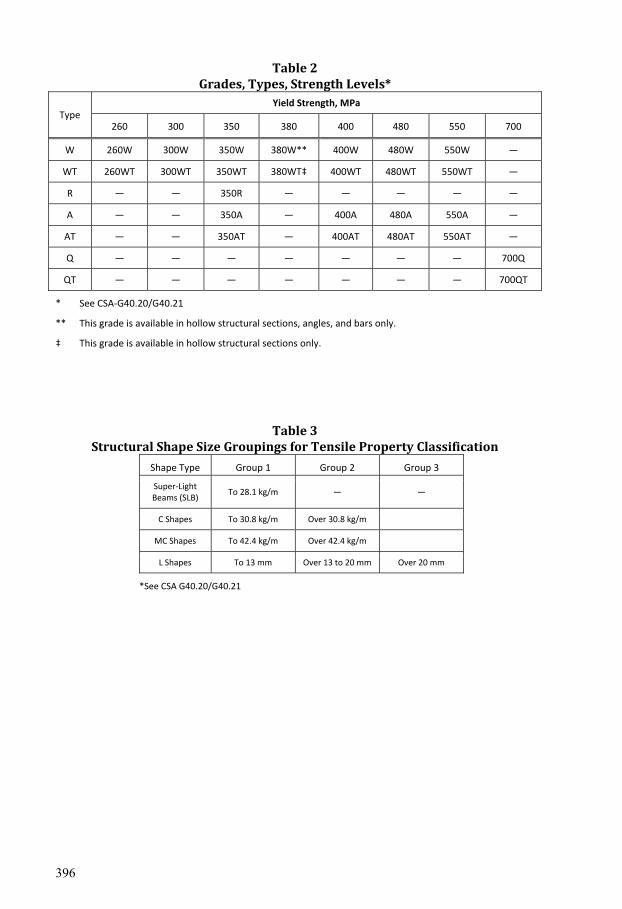
Table 2

Grades, Types, Strength Levels*

Type Yield Strength, MPa

260 300 350 380 400 480 550 700

W 260W 300W 350W 380W** 400W 480W 550W —

WT 260WT 300WT 350WT 380WT‡ 400WT 480WT 550WT —

R — — 350R — — — — —

A — — 350A — 400A 480A 550A —

AT — — 350AT — 400AT 480AT 550AT —

Q — — — — — — — 700Q

QT — — — — — — — 700QT

* See CSA-G40.20/G40.21

** This grade is available in hollow structural sections, angles, and bars only.

‡ This grade is available in hollow structural sections only.

Table 3 Structural Shape Size Groupings for Tensile Property Classification

Shape Type Group 1 Group 2 Group 3

Super-Light Beams (SLB) To 28.1 kg/m — —

C Shapes To 30.8 kg/m Over 30.8 kg/m

MC Shapes To 42.4 kg/m Over 42.4 kg/m

L Shapes To 13 mm Over 13 to 20 mm Over 20 mm

*See CSA G40.20/G40.21

397

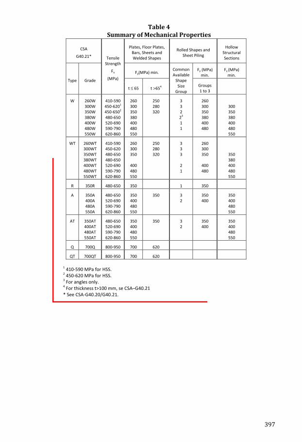
Table 4 Summary of Mechanical Properties

CSA

G40.21* Tensile Strength

Fu

(MPa)

Plates, Floor Plates, Bars, Sheets and Welded Shapes

Rolled Shapes and Sheet Piling

Hollow Structural Sections

Type Grade

Fy(MPa) min. Common Available

Shape Size

Group

Fy (MPa) min.

Fy (MPa) min.

t ≤ 65 t >654 Groups 1 to 3

W 260W 300W 350W 380W 400W 480W 550W

410-590450-6201

450-6502

480-650520-690590-790620-860

260 300 350 380 400 480 550

250 280 320

3 3 2 23 1 1

260 300 350 380 400 480

300 350 380 400 480 550

WT 260WT 300WT 350WT 380WT 400WT 480WT 550WT

410-590450-620480-650480-650520-690590-790620-860

260 300 350

400 480 550

250 280 320

3 3 3

2 1

260 300 350

400 480

350 380 400 480 550

R 350R 480-650 350 1 350

A 350A 400A 480A 550A

480-650520-690590-790620-860

350 400 480 550

350 3 2

350 400

350 400 480 550

AT 350AT 400AT 480AT 550AT

480-650520-690590-790620-860

350 400 480 550

350 3 2

350 400

350 400 480 550

Q 700Q 800-950 700 620

QT 700QT 800-950 700 620

1 410-590 MPa for HSS. 2 450-620 MPa for HSS. 3 For angles only. 4 For thickness t>100 mm, se CSA–G40.21 * See CSA-G40.20/G40.21.