Hydrobiologia 502: 13–36, 2003.L. Naselli-Flores, J. Padisak, M. T. Dokulil (eds),Phytoplankton and Equilibrium Concept: The Ecology of Steady-State Assemblages.© 2003 Kluwer Academic Publishers. Printed in the Netherlands.

13

Life strategies, dominance patterns and mechanisms promoting speciescoexistence in phytoplankton communities along complex environmentalgradients

Nico SalmasoDipartimento di Biologia, Universita di Padova, Via U. Bassi 58/B, I-35131 Padova, ItalyE-mail: nico.salmaso@unipd.it

Key words: phytoplankton, ecological niches, community change rate, complex environmental gradients,multivariate analyses, deep lakes

Abstract

This paper analyses the life strategies, the dominance patterns and the diversity in phytoplankton communitiesin large and deep lakes. The study was carried out on the largest Italian Lake (Lake Garda) from 1995 to 2000.Different statistical analyses were applied. For phytoplankton the time variable represents a complex environmentalgradient driving annual succession; this gradient was made explicit by the application of PCA analyses to the en-vironmental data. The use of Non Metric Multi Dimensional Scaling applied to Bray-Curtis dissimilarity matricesrevealed an ordered and cyclic development of phytoplankton every year; the Bray-Curtis index, calculated betweenpairs of chronologically contiguous samples, was also used as a measure of the community change rate (β t) over thetemporal succession. A significant relationship between β t and the complex environmental gradient was assessed.Finally, for every phytoplankton species, the optimum conditions for growth and the realised niches were determ-ined. The positioning of the species on the complex environmental gradient, and the contemporaneous applicationof cluster analysis based on the different specific environmental optima, highlighted primarily the existence of twogroups at the extreme of the complex environmental gradient. The first group included the large late winter/springdiatoms, which developed during high water turbulence and strong physical control, high nutrient concentrations,low light conditions and reduced competition. The second group was composed by many heterogeneous summerspecies characterised by the ability to contrast losses by grazing and sinking in stratified and stable conditions, andthe ability of tolerating nutrient deficiency. A third group of species developed during environmental conditionsin the middle of the two previous extremes. These included the three master species Mougeotia sp., Fragilariacrotonensis and Planktothrix rubescens/agardhii. The endogenous and exogenous mechanisms promoting speciescoexistence are discussed, along with the applicability of competitive and equilibrium/non-equilibrium theories tophytoplankton dynamics.

Introduction

Phytoplankton communities in lakes are composedof many different species. Sometimes dominants andsubdominants may be evidenced, along with sev-eral rare species coexisting with the more abundantones; a similar experience is provided by many areascovered by herbaceous or forest vegetation (Hutchin-son, 1967).

Most phytoplankton species are potential compet-itors for the same limited resources of their envir-

onment (principally nutrients and light). Under suchconditions, the high number of coexisting speciescontrasts largely with the results that can be pre-dicted from the application of competition theories.The Competitive Exclusion Principle (Gause’s Prin-ciple) states that two or more species cannot coexist ifthey make use of the same limiting resources, namely‘complete competitors cannot coexist’ (Hardin, 1960)and each community should be dominated by veryfew species occupying different niches. Niche is in-tended in the sense of Hutchinson (1967), designating

14

the requirements of an organism abstracted from thespatially extended habitat. However, competitive dom-inance of the best adapted species is a process requir-ing a homogeneous habitat, environmental stabilityand equilibrium conditions; if communities developin non-equilibrium conditions, then competitive exclu-sion is prevented. Hutchinson (1961) proposed that thecoexistence of many species of phytoplankton couldbe due to environmental instability preventing equi-librium. Therefore, phytoplankton may be viewedas a non-equilibrium community of competing spe-cies and thus are not an exception to the principle ofcompetitive exclusion (Krebs, 2001).

Considering the high potential reproductive ratesof phytoplankton organisms (with doubling timesspanning from fractions of days to few days), environ-mental instability comprises factors characterised byvery different temporal scales. Some factors act onshort-medium time (i.e. days–weeks; e.g., meteoro-logical and hydrological events, grazing, vertical andhorizontal chemical gradients), while others evolveregularly on seasonal basis (e.g., changes in solarradiation, development and breaking of thermal strat-ification, replenishment and depletion of nutrients,seasonality of zooplankton grazers). The first groupof factors – depending on the intensity and on the fre-quency of disturbances – is instrumental for support-ing non-equilibrium dynamics and diversity (Connell,1978; Padisák, 1994) or fast community reorganisa-tion events (reversions or catastrophes). As for thesecond group of factors, the annual evolution of solarelevation in the medium and high latitude regionsis crucial to determine the seasonal replacement ofphytoplankton assemblages. In fact, for phytoplankton– and other organisms responding in a similar way tothe same temporal scales – the time variable repres-ents a complex environmental gradient driving annualsuccessions. Different life history traits determine thesuccess of different species at a particular region ofany environmental gradient. When these traits (e.g.,growth rates, nutrient requirements, shade toleranceetc.) are inversely correlated, successional replace-ment will result (McCook, 1994). On annual basis,the two temporally scaled groups of factors causinginstability and environmental seasonal change are es-sential in supporting the diversity of phytoplankton(the ‘species richness’ of a waterbody). In a givenhabitat it is convenient to consider different compon-ents in species diversity (e.g., Whittaker, 1972). Theseinclude the richness in species of a given sample (αdiversity) and the biological diversity along habitat

gradients (e.g., elevation or soil moisture: β diversity).Excluding particular cases (e.g., the world’s largestfreshwater ecosystems, Bondarenko et al., 1996), themain differences in the composition of phytoplanktonin the pelagic zone of the lakes evolve along temporalgradients. In this work, the extent of differentiationof the community along the temporal gradient will beindicated as βt .

The relative importance of the two groups offactors determining environmental instability andchange, as well as total phytoplankton diversity in agiven waterbody, is mediated by the peculiar morpho-metric and hydrological characteristics of the differenttypes of lakes. Large and deep lakes have the tendencyto operate as large inertial systems, for they minimisethe effect of external disturbances. Previous investiga-tions carried out during the 1990s in the largest Italianlake (Lake Garda) revealed an ordered and coherenttemporal succession of phytoplankton assemblagesin the whole basin (Salmaso, 1996, 2002). On thecontrary, the seasonal sequence of phytoplankton spe-cies in lakes located at the opposite morphometricand hydrological gradient (e.g., small and shallowmountain lakes) may be strongly influenced by met-eorological (rains and storms) and hydrological events(snow melting, high water flushing or drought in thewarm period), with different species being domin-ant in various years (Salmaso & Decet, 1997). Thevariations concerning phytoplankton tend to be morepredictable in large inertial systems, because theyare more dependent on the annual evolution of theenvironmental climatic forcing variables, and less de-pendent on stochastic events. Disturbances classifiedas ‘strong’ for small and shallow lakes may have littleconsequences for largest basins.

In this work, I will compare the specific envir-onmental requirements and life strategies of differentalgae, in order to explain their seasonal (successional)adaptation and dominance along temporal gradientsin deep and large lakes. The specific objectives ofthis paper are: (i) to define the average, typicalannual development and apparent optimum environ-mental conditions for growth of the most abundantphytoplankton species in the deep and large LakeGarda, based on 6 years of studying; (ii) to investig-ate the correlations between the temporal evolution ofthe main environmental factors and species turnover(βt ) and (iii) to discuss the seasonal changes in thedominant assemblages along complex environmentalgradients, taking into account the specific competit-ive abilities defined for the most abundant taxa, and

15

evidencing the exogenous and endogenous factors pro-moting phytoplankton diversity and species turnover.The relevance of the above topics will be emphasisedin relation to the applicability of equilibrium conceptsto phytoplankton dynamics. Hereafter the term ‘com-munity’ will be used to indicate the whole pool ofspecies present in an annual cycle, i.e. the potentialcompetitors and winners along the temporal gradi-ent, whereas ‘assemblage’ will be used to indicate ageneric seasonal phytoplankton group.

Study site

Lake Garda is the largest Italian lake. Along with thelakes Iseo, Como, Lugano and Maggiore, it is one ofthe deep lakes (Insubrian lakes) located south of theAlps. Lake Garda has a volume of 49 km3, a surfaceof 368 km2 and a maximum depth of 350 m. Thelong theoretical water renewal time (27 years) is dueto its low catchment (lake included)/lake surface ratio(around 6) and to low annual rainfall (790–1150 mm,IRSA, 1974). The main inflow is River Sarca, at thenorthern edge of the lake. The outflow, with an av-erage discharge of 58 m3 s−1, is River Mincio, at thesouthern edge of the lake. Details of the catchment andthe lake are reported in IRSA (1974).

Materials and methods

Methods in the field and laboratory

The data refer to samples collected normally everyfour weeks between January 1995 and December 2000in the deepest zone of the lake (west basin, Bren-zone). The average values of the chemical variablesand phytoplankton abundance in the upper 20 m wereestimated from samples collected at discrete depths.

From 1996 to 2000, water samples for phytoplank-ton analyses were collected at the integrated depths of0–2 m, 9.5–11.5 m and 19–21 m with a 5 l, 0.5 mlong Niskin bottle (for a total final volume of 20 l);in 1995 samplings were not carried out in the middlelayer (9.5–11.5 m). Chlorophyll a was determined byspectrophotometry following the methods proposedby Lorenzen (1967). Subsamples of 200 ml werefixed with Lugol’s solution and stored in bottles ofglass kept in the dark at 4 ◦C for subsequent phyto-plankton analyses. Algal cells were counted usinginverted microscopes, following the criteria reported

by Lund et al. (1958). The counts include, besides theidentified fraction, ultraplankton (naked or flagellatecells around 4 µm) and undetermined nanoflagellates(around 5–10 µm). A detailed description of the pro-cedures used in the laboratory is reported by Salmaso(2002).

Water samples for chemical analyses were collec-ted at the surface and at 20 m depths, with the excep-tion of December 2000. Soluble reactive (RP) and totalphosphorus (TP), nitrate (NO3-N) and ammonium ni-trogen (NH4-N), reactive silica and pH have beenmeasured by the Veneto Region Environment Protec-tion Agency (ARPAV, District of Belluno) followingstandard methods (APHA et al., 1989). The analyticalprocedures are described by Decet & Salmaso (1997).

On each sampling, profiles of temperature werecarried out with an underwater multiparameter probe.The differences of water density between 0–20 m(�δ0−20) and 0–150 m (�δ0−150) were taken as meas-ures of the water column stability in the layer sampledfor phytoplankton analyses and in the mixolimnion,respectively. Water density was computed from tem-perature measurements (Chen & Millero, 1986).

Secchi disk transparency (zs) was estimated usinga bathiscope to reduce uncertainties in the measure-ments due to light reflections and wave motions. Theeuphotic depth (zeu) was estimated from Secchi discreadings using the relationship:

Zeu = 4.8 × Z0.68S

(Salmaso, 2002).The measurements of total solar radiation were

obtained at the Agricultural Institute of S. Micheleall’Adige (Section of Agrometeorology, publicallyavailable information). The measurement station waslocated at Arco, at the northern border of the lake,approximately 25 km away from the sampling station.As a measure of light availability for phytoplanktongrowth, the average values of solar radiation during the3 days prior to sampling dates (I3d) were considered(cf. Bleiker & Schanz, 1997). In only few cases, miss-ing observations were supplied with the correspondingmeasurements made at S. Michele all’Adige (35 kmfrom Arco). The 3-day averages were compared withthe average annual solar radiation trend at Arco, ob-tained on the basis of fortnightly averages computedfor the period 1983–2000.

16

Data analysis

Individual samples were ordered by principal compon-ents analysis (PCA) calculated from the correlationmatrix of the physical and chemical untransformedvariables.

Biovolume based Shannon (H′) diversity (α di-versity) was estimated using natural logarithms(Magurran, 1988); unidentified ultraplankton and nan-oflagellates were not considered in the calculation.Phytoplankton data were analysed by Nonmetric Mul-tidimensional Scaling (NMDS) (Kruskal & Wish,1978; Salmaso, 1996); the ordinations were appliedto Bray & Curtis’ dissimilarity matrices (Bray &Curtis, 1957) computed on biovolume values. Uniden-tified phytoplankton and rare species found in oneoccasion were neglected. Double square root trans-formation of the original data was applied to reducethe weight of the most abundant species (Field etal., 1982). The Bray-Curtis dissimilarity calculatedbetween pairs of chronologically contiguous samples,was also used as an estimate of the differentiationof the community along the complex environmentalgradient (community change rate, βt ) (cf. Whittaker,1972; Salmaso, 1996).

The single species were placed on the complexenvironmental gradient defined by the first two PCAaxes (cf. Fabbro & Duivenvoorden, 2000) taking intoaccount their biovolume variations (cf. Bray & Curtis,1957) (Fig. 7). Each taxon k has been located com-puting the average values – weighted by the corres-ponding biovolume values – of the coordinates of thesamples where it was determined. For the coordinatesalong the horizontal axis, xk is:

xk =n∑

i=1

bikXi

/ n∑i=1

bik

where xk is the value of the coordinate of species kon the first PCA axis, bik the abundance of taxon k insample i (bik ≥ 0), xi the value of the coordinate ofsample i on the first PCA axis (cf. Fig. 2) and n thenumber of samples (n = 75).

For every species, the observed optimum environ-mental conditions for growth were computed – analog-ously to the previous formula – by weighted averagingestimates (ter Braak & van Dam, 1989). A species kwith a particular optimum for a variable, will be mostabundant in samples where this variable is close toits optimum. The weighted averaging estimate of the

optimum uk is:

uk =n∑

i=1

bikvi

/ n∑i=1

bik

and the species’ tolerance, tk , or weighted standarddeviation, is:

tk =[

n∑i=1

bik(vi − uk)2/ n∑

i=1

bik

]1/2

where bik is the biovolume of taxon k in sample i(bik ≥ 0) and vi the value of the variable of interestin sample i; the computations were carried out on thewhole set of samples (n = 76 or, in the case of algalnutrients, n = 75).

Finally, the optimum values (uk) were utilised toidentify the principal life strategies, classifying thephytoplankton species by cluster analysis (Pearsondistance, Ward’s method).

Phytoplankton diversity and dissimilarity indiceswere computed with SIMDISS 2.0 (http://www.bio.unipd.it/limno/simdiss/), whereas multivariate analyseswere carried out with SYSTAT packages.

Results

Physical and chemical variables

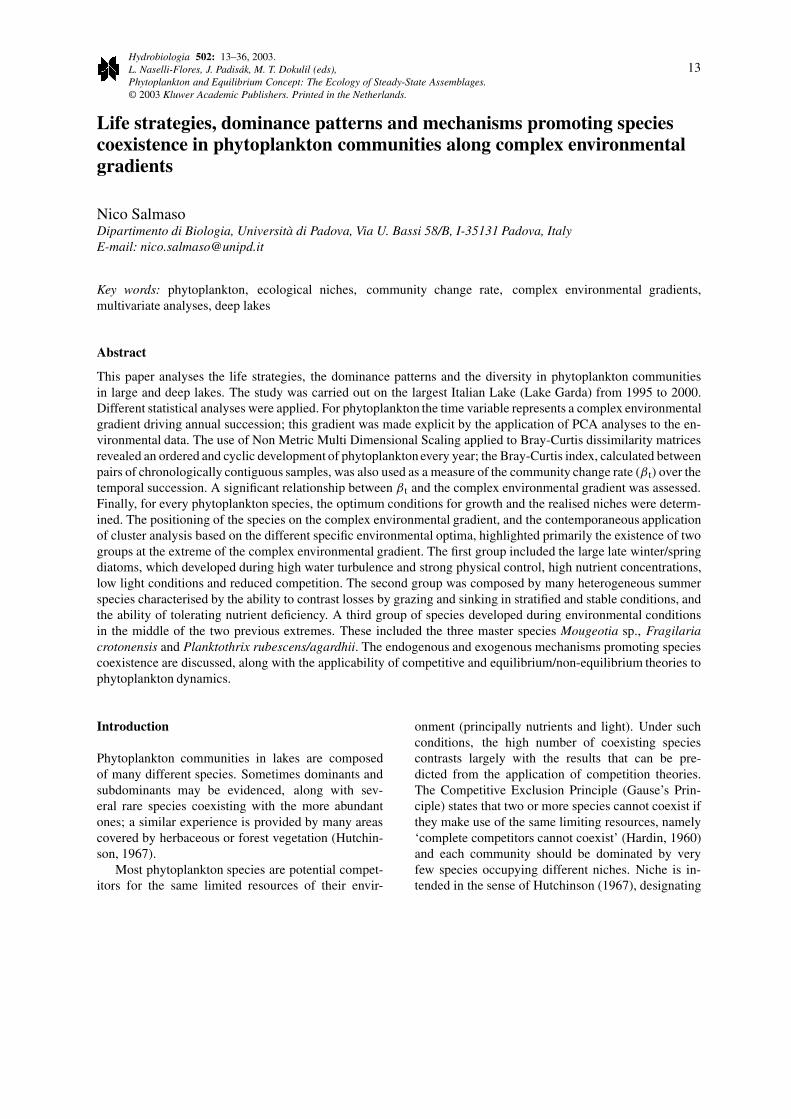
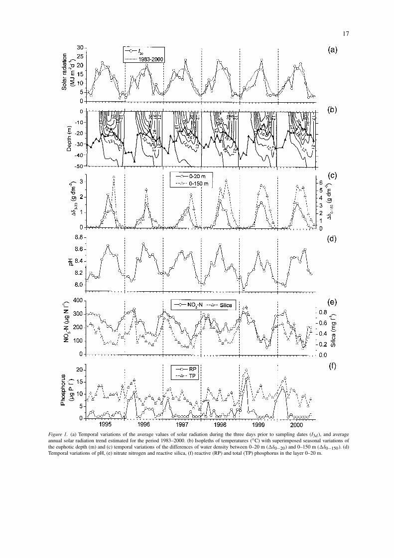
The principal environmental abiotic variables affect-ing the seasonal evolution of the phytoplankton com-munity are reported in Figure 1.

Solar radiation (I3d ) showed an annual oscillation,with values ranging from 2.5–5 MJ m−2 d−1 to 20–25 MJ m−2 d−1 (Fig. 1a). Some differences emergedfrom the comparison of the I3d values with the averageannual solar radiation trend (1983–2000). However,the 3-day averages were strongly correlated with thecorresponding averages computed during the week be-fore the sampling (7-day averages; r = 0.94; P < 0.01),so they seem to represent quite well the available in-come radiation for the growth of phytoplankton in adetermined period of the annual cycle.

From late spring to early autumn the lake dis-played a marked thermal stratification. Maximumtemperatures in the first metre reached 22–25 ◦C,whereas the metalimnetic layer deepened down to 30–40 m (Fig. 1b). The maximum winter euphotic depthsranged around 30–45 m (Fig. 1b). During summer, thelower limit of the euphotic layer was located between

17

Figure 1. (a) Temporal variations of the average values of solar radiation during the three days prior to sampling dates (I3d ), and averageannual solar radiation trend estimated for the period 1983–2000. (b) Isopleths of temperatures (◦C) with superimposed seasonal variations ofthe euphotic depth (m) and (c) temporal variations of the differences of water density between 0–20 m (�δ0−20) and 0–150 m (�δ0−150). (d)Temporal variations of pH, (e) nitrate nitrogen and reactive silica, (f) reactive (RP) and total (TP) phosphorus in the layer 0–20 m.

18

15 and 25 m from 1995 to 1998, and between 11and 20 m in 1999 and 2000. The euphotic depthshowed similar or greater values than the mixing depth(zeu/zmix ≥ 1) from May-June to September.

In the layer 0–20 m complete mixing (�δ0−20 = 0 gdm−3) was generally observed in the period betweenOctober–November and March–April (Fig. 1c); thehigher stability of the water column (�δ0−20 >

1 g dm−3) was observed between June-July and Au-gust. The isopycnic layer extended down to 150 m(�δ0−150 ∼= 0 g dm−3) between December andMarch–April. This layer may be roughly consideredthe mixolimnion of the lake, because it undergoesthermal cooling and mixing during the late winter andearly spring months. During the 1990s, complete ver-tical cooling (down to 350 m) and circulation wasdocumented only in 1999 and 2000 (Salmaso et al.,2001).

The seasonality of pH and nutrients is relatedto higher phytoplankton growth during the summermonths and also to the vertical mixing of the watercolumn occurring from late autumn to early spring.In the layer 0–20 m the pH values showed a regularseasonal evolution, with values ranging from 7.9 to 8.7(Fig. 1d).

Nitrate nitrogen and silica decreased together dur-ing the warmest months (Fig. 1e; r = 0.68; P < 0.01).The lower concentrations of NO3-N in the 20-m layerwere around 120–175 µg N l−1 from 1995 to 1998,and 60–70 µg N l−1 in 1999 and 2000. The minimumSi concentrations fluctuated from 0.15 to 0.25 mg Sil−1 in the whole case study. After the minimum sum-mer values, the epilimnetic increase of NO3-N and Siconcentrations took place with the deepening of themixing layer (Fig. 1c). NH4-N concentrations weregenerally below 20 µg N l−1 and contributed onlysecondarily to the total amount of nitrogen.

In 1999 and 2000, reactive and total phosphorusshowed higher concentrations (up to 20 µg P l−1 ofTP in 1999) in comparison to those measured in 1995–1998 (Fig. 1f). These differences were caused by thedifferent extent of the spring vertical mixing, whichdetermined a major recycling of phosphorus from thedeepest layers to the surface during the 2 years (1999–2000) of complete overturn (Salmaso et al., 2001).A clear influence of the extent of the vertical watermixing was not evident for Si and NO3-N.

Table 1. (a) Principal components analyses computed on the ori-ginal physical and chemical variables and (b) on the same setof variables averaged over two consecutive samples. The twopanels show the percentage of explained variance and the correl-ations between the first two components and the input variables.Significant correlations are reported in bold (P<0.01) and italic(P<0.05)

(a) (b)

PCA Axis I II I II

Variance explained 64.8% 13.7% 68.7% 12.8%

T0−20 0.93 0.00 0.93 –0.06

pH 0.87 0.09 0.89 0.13

�δ0−20 0.81 0.46 0.84 0.43I3d 0.61 0.68 0.66 0.68zeu –0.87 0.13 –0.91 0.09

NO3-N –0.85 0.23 –0.85 0.26

Si –0.83 0.29 –0.84 0.29

RP –0.62 0.51 –0.67 0.47

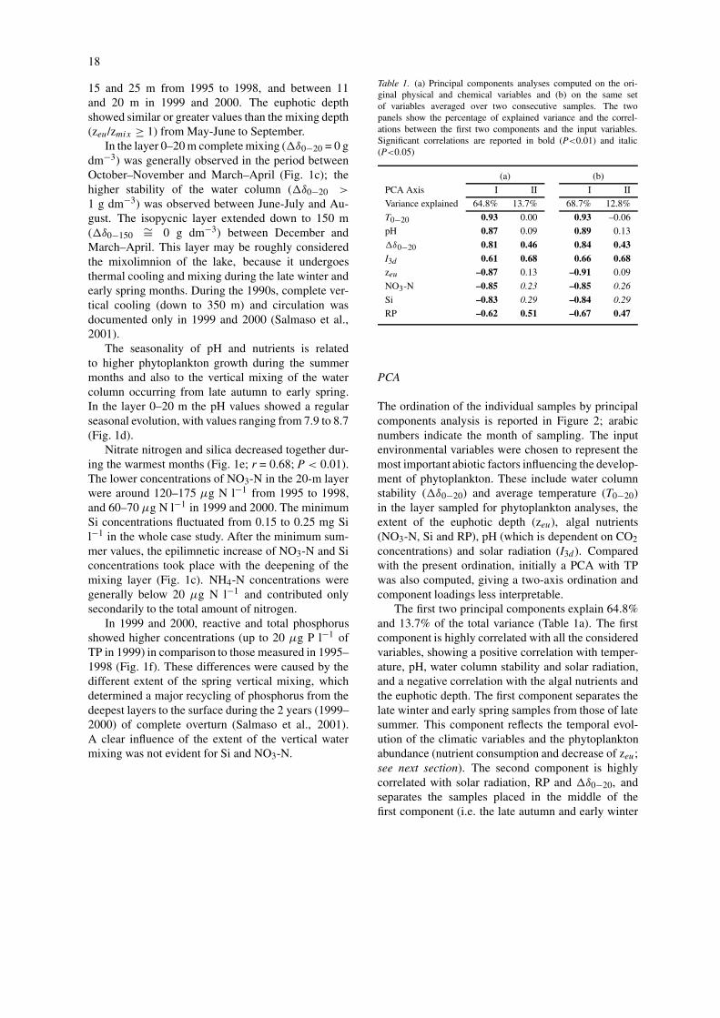
PCA

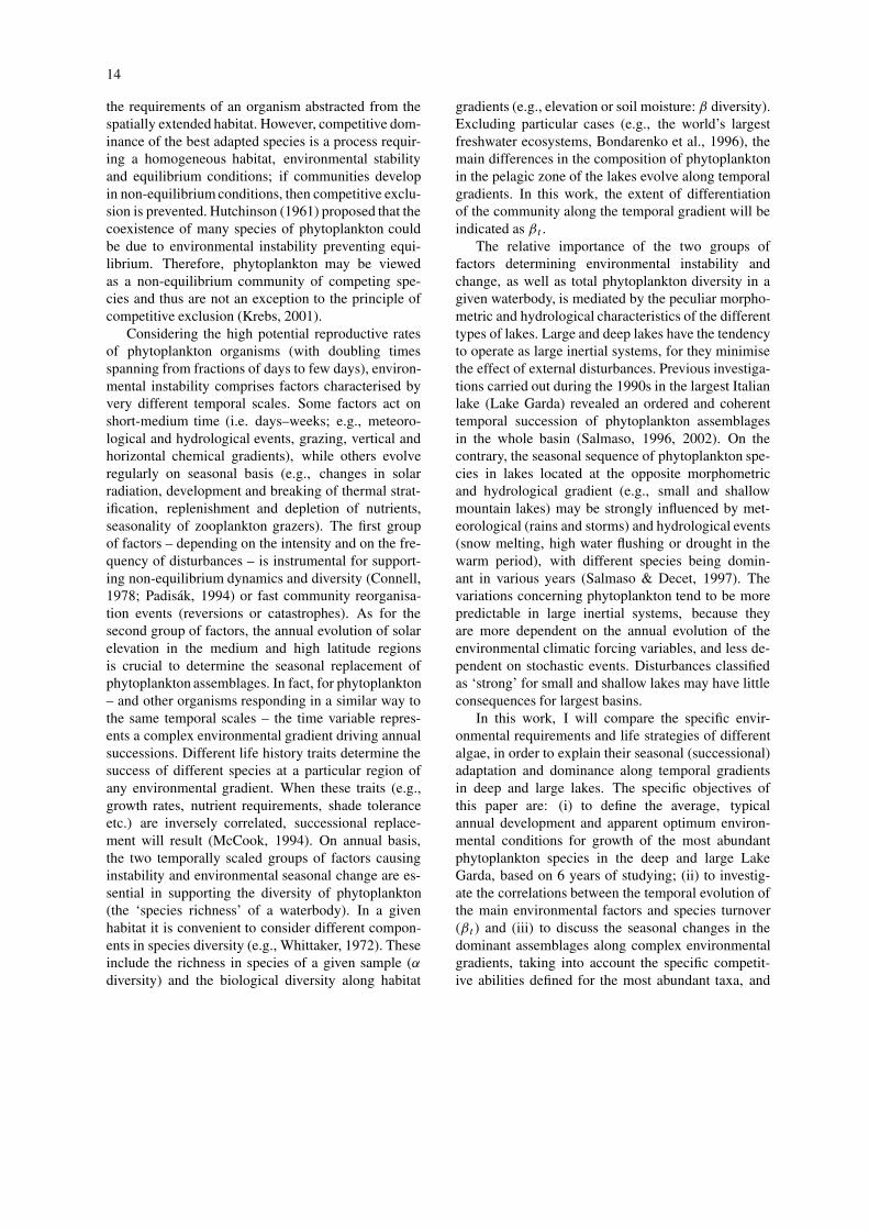
The ordination of the individual samples by principalcomponents analysis is reported in Figure 2; arabicnumbers indicate the month of sampling. The inputenvironmental variables were chosen to represent themost important abiotic factors influencing the develop-ment of phytoplankton. These include water columnstability (�δ0−20) and average temperature (T0−20)in the layer sampled for phytoplankton analyses, theextent of the euphotic depth (zeu), algal nutrients(NO3-N, Si and RP), pH (which is dependent on CO2concentrations) and solar radiation (I3d ). Comparedwith the present ordination, initially a PCA with TPwas also computed, giving a two-axis ordination andcomponent loadings less interpretable.

The first two principal components explain 64.8%and 13.7% of the total variance (Table 1a). The firstcomponent is highly correlated with all the consideredvariables, showing a positive correlation with temper-ature, pH, water column stability and solar radiation,and a negative correlation with the algal nutrients andthe euphotic depth. The first component separates thelate winter and early spring samples from those of latesummer. This component reflects the temporal evol-ution of the climatic variables and the phytoplanktonabundance (nutrient consumption and decrease of zeu;see next section). The second component is highlycorrelated with solar radiation, RP and �δ0−20, andseparates the samples placed in the middle of thefirst component (i.e. the late autumn and early winter

19

Figure 2. Ordination of samples by principal components analysis; arabic numbers refer to the sampling months. The correlations of theoriginal variables with the two principal components (Table 1a) are highlighted. The circles corresponding to consecutive centroids of thedifferent months have been joined with a continuous line.

samples from those of late spring and early summer);this component shows only a slight correlation with Siand NO3-N (Table 1a). The second axis reflects theeffects of the annual climatic evolution, along with the‘residual’ high availability, and low concentrations ofRP after the spring overturn and the autumn months,respectively. Overall, the plane defined by the first twocomponents describes a complex environmental gradi-ent, expressed by the combination of the consideredvariables.

The temporal path of the individual samples fol-lows an annual cycle. This becomes clearer taking intoaccount the seasonal evolution of the centroids of thedifferent months, whose position in Figure 2 was de-termined by computing the monthly averages of thecoordinates xi and yi for the complete set of samples.

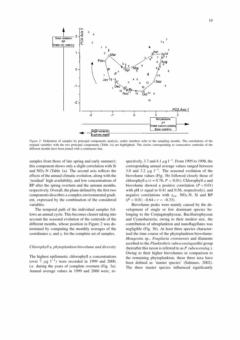
Chlorophyll a, phytoplankton biovolume and diversity

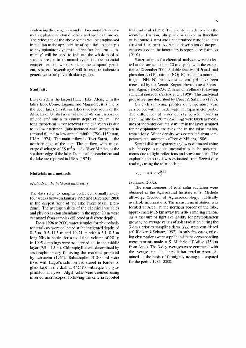
The highest epilimnetic chlorophyll a concentrations(over 7 µg l−1) were recorded in 1999 and 2000,i.e. during the years of complete overturn (Fig. 3a).Annual average values in 1999 and 2000 were, re-

spectively, 3.7 and 4.1 µg l−1. From 1995 to 1998, thecorresponding annual average values ranged between3.0 and 3.2 µg l−1. The seasonal evolution of thebiovolume values (Fig. 3b) followed closely those ofchlorophyll a (r = 0.78; P < 0.01). Chlorophyll a andbiovolume showed a positive correlation (P < 0.01)with pH (r equal to 0.41 and 0.56, respectively), andnegative correlations with zeu, NO3-N, Si and RP(P < 0.01; –0.64< r < –0.33).

Biovolume peaks were mainly caused by the de-velopment of single or few dominant species be-longing to the Conjugatophyceae, Bacillariophyceaeand Cyanobacteria; owing to their modest size, thecontribution of ultraplankton and nanoflagellates wasnegligible (Fig. 3b). At least three species character-ised the time course of the phytoplankton biovolume:Mougeotia sp., Fragilaria crotonensis and filamentsascribed to the Planktothrix rubescens/agardhii group(hereafter this taxon is referred to as P. rubescens/ag.).Owing to their higher biovolumes in comparison tothe remaining phytoplankton, these three taxa havebeen defined as ‘master species’ (Salmaso, 2002).The three master species influenced significantly

20

Figure 3. (a) Temporal variations of chlorophyll a. (b) Biovolume variations of phytoplankton subdivided by algal groups and ultraplank-ton/nanoflagellates in the layer 0–21 m. (c) Temporal variations of Shannon diversity computed for the whole phytoplankton community (H′)and disregarding the contribution of the three master species Mougeotia sp., F. crotonensis and P. rubescens/ag. (H′

sub ).

(P < 0.01) the temporal evolution of the biovolumesof their corresponding algal classes, with correlationcoefficients r equal to 0.997 (Mougeotia sp. vs. con-jugatophytes), 0.91 (F. crotonensis vs. diatoms), and0.89 (P. rubescens/ag. vs. cyanobacteria). Together,these three taxa strongly determined the time courseof the total biovolume (r = 0.91; P < 0.01). Mougeo-tia sp. developed regularly in the period from springto early autumn; F. crotonensis was mainly presentduring the spring or autumn months, but with ir-regular, significant biovolumes also in the remainingperiods; P. rubescens/ag. developed mostly in summerand autumn, with populations persisting in winter andspring.

Phytoplankton diversity showed a regular temporalevolution (Fig. 3c). With few exceptions (e.g., Decem-ber 1995), maximum values were found from summerto winter. The time course of diversity was stronglyaffected by the development of the most abundanttaxa. In particular, the elevated growth of Mougeo-tia sp. in spring and early summer was important forthe decrease of diversity. On the other side, diversitywas sustained by the seasonal development of manyother dominant or subdominant species. The Shan-

non index computed disregarding the contribution ofMougeotia sp., F. crotonensis and P. rubescens/ag.(H′

sub) showed greater values in comparison withthose calculated on the whole data matrix.

Seasonal evolution of the phytoplankton community

Besides the three master species, many other taxabecame important along the annual temporal gradi-ent. A group of species, with biovolume peaks >

50 mm3 m−3, was distinguished from the remain-ing taxa. These species belong to the Bacillario-phyceae (Asterionella formosa, Aulacoseira granu-lata, A. islandica, Cyclotella spp., Stephanodiscussp. and Tabellaria fenestrata), Conjugatophyceae(Closterium aciculare and C. pronum), Chloro-phyceae (Coelastrum spp., Ulothrix sp. and Ulo-thrichales), Cyanobacteria (Limnotrichoideae (Limno-thrix sp. ?) sensu Anagnostidis & Komárek (1988),Microcystis aeruginosa and Planktolyngbya limnet-ica), Chrysophyceae (Dinobryon divergens, D. socialeand Ochromonadaceae), Cryptophyceae (Plagioselmisnannoplanctica (Novarino et al., 1994) (which, inLake Garda, was previously reported as Chroomo-

21

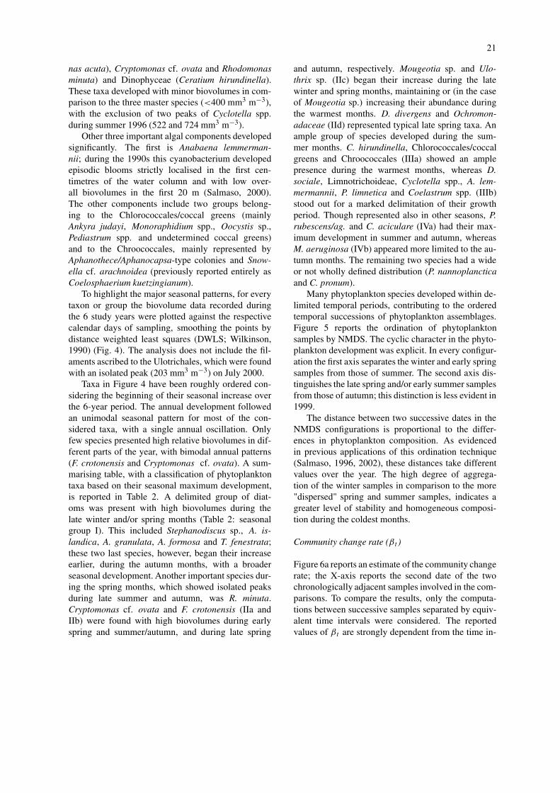
nas acuta), Cryptomonas cf. ovata and Rhodomonasminuta) and Dinophyceae (Ceratium hirundinella).These taxa developed with minor biovolumes in com-parison to the three master species (<400 mm3 m−3),with the exclusion of two peaks of Cyclotella spp.during summer 1996 (522 and 724 mm3 m−3).

Other three important algal components developedsignificantly. The first is Anabaena lemmerman-nii; during the 1990s this cyanobacterium developedepisodic blooms strictly localised in the first cen-timetres of the water column and with low over-all biovolumes in the first 20 m (Salmaso, 2000).The other components include two groups belong-ing to the Chlorococcales/coccal greens (mainlyAnkyra judayi, Monoraphidium spp., Oocystis sp.,Pediastrum spp. and undetermined coccal greens)and to the Chroococcales, mainly represented byAphanothece/Aphanocapsa-type colonies and Snow-ella cf. arachnoidea (previously reported entirely asCoelosphaerium kuetzingianum).

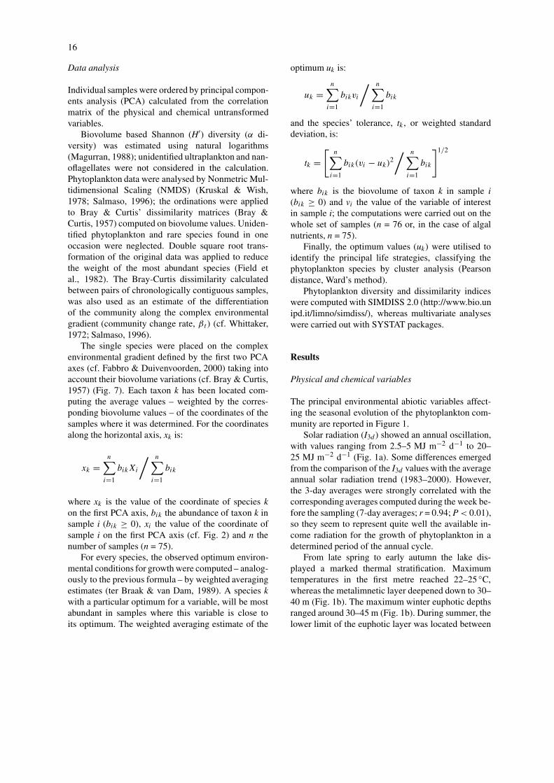
To highlight the major seasonal patterns, for everytaxon or group the biovolume data recorded duringthe 6 study years were plotted against the respectivecalendar days of sampling, smoothing the points bydistance weighted least squares (DWLS; Wilkinson,1990) (Fig. 4). The analysis does not include the fil-aments ascribed to the Ulotrichales, which were foundwith an isolated peak (203 mm3 m−3) on July 2000.

Taxa in Figure 4 have been roughly ordered con-sidering the beginning of their seasonal increase overthe 6-year period. The annual development followedan unimodal seasonal pattern for most of the con-sidered taxa, with a single annual oscillation. Onlyfew species presented high relative biovolumes in dif-ferent parts of the year, with bimodal annual patterns(F. crotonensis and Cryptomonas cf. ovata). A sum-marising table, with a classification of phytoplanktontaxa based on their seasonal maximum development,is reported in Table 2. A delimited group of diat-oms was present with high biovolumes during thelate winter and/or spring months (Table 2: seasonalgroup I). This included Stephanodiscus sp., A. is-landica, A. granulata, A. formosa and T. fenestrata;these two last species, however, began their increaseearlier, during the autumn months, with a broaderseasonal development. Another important species dur-ing the spring months, which showed isolated peaksduring late summer and autumn, was R. minuta.Cryptomonas cf. ovata and F. crotonensis (IIa andIIb) were found with high biovolumes during earlyspring and summer/autumn, and during late spring

and autumn, respectively. Mougeotia sp. and Ulo-thrix sp. (IIc) began their increase during the latewinter and spring months, maintaining or (in the caseof Mougeotia sp.) increasing their abundance duringthe warmest months. D. divergens and Ochromon-adaceae (IId) represented typical late spring taxa. Anample group of species developed during the sum-mer months. C. hirundinella, Chlorococcales/coccalgreens and Chroococcales (IIIa) showed an amplepresence during the warmest months, whereas D.sociale, Limnotrichoideae, Cyclotella spp., A. lem-mermannii, P. limnetica and Coelastrum spp. (IIIb)stood out for a marked delimitation of their growthperiod. Though represented also in other seasons, P.rubescens/ag. and C. aciculare (IVa) had their max-imum development in summer and autumn, whereasM. aeruginosa (IVb) appeared more limited to the au-tumn months. The remaining two species had a wideor not wholly defined distribution (P. nannoplancticaand C. pronum).

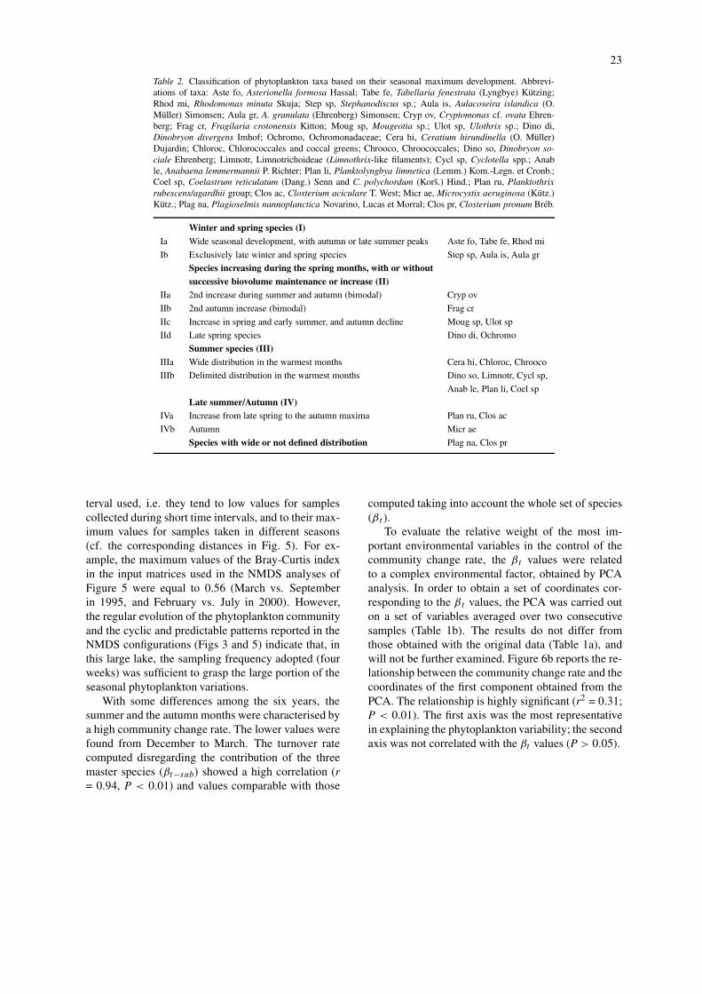
Many phytoplankton species developed within de-limited temporal periods, contributing to the orderedtemporal successions of phytoplankton assemblages.Figure 5 reports the ordination of phytoplanktonsamples by NMDS. The cyclic character in the phyto-plankton development was explicit. In every configur-ation the first axis separates the winter and early springsamples from those of summer. The second axis dis-tinguishes the late spring and/or early summer samplesfrom those of autumn; this distinction is less evident in1999.

The distance between two successive dates in theNMDS configurations is proportional to the differ-ences in phytoplankton composition. As evidencedin previous applications of this ordination technique(Salmaso, 1996, 2002), these distances take differentvalues over the year. The high degree of aggrega-tion of the winter samples in comparison to the more"dispersed" spring and summer samples, indicates agreater level of stability and homogeneous composi-tion during the coldest months.

Community change rate (βt )

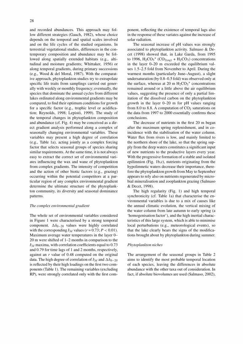
Figure 6a reports an estimate of the community changerate; the X-axis reports the second date of the twochronologically adjacent samples involved in the com-parisons. To compare the results, only the computa-tions between successive samples separated by equiv-alent time intervals were considered. The reportedvalues of βt are strongly dependent from the time in-

22

Figure 4. Annual distribution of biovolume values (mm3 m−3) for the most abundant taxa. Data refer to the period 1995–2000. The pointswere smoothed by distance weighted least squares (DWLS).

23

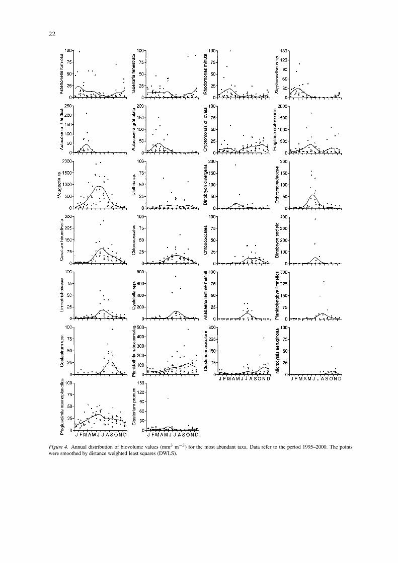
Table 2. Classification of phytoplankton taxa based on their seasonal maximum development. Abbrevi-ations of taxa: Aste fo, Asterionella formosa Hassal; Tabe fe, Tabellaria fenestrata (Lyngbye) Kützing;Rhod mi, Rhodomonas minuta Skuja; Step sp, Stephanodiscus sp.; Aula is, Aulacoseira islandica (O.Müller) Simonsen; Aula gr, A. granulata (Ehrenberg) Simonsen; Cryp ov, Cryptomonas cf. ovata Ehren-berg; Frag cr, Fragilaria crotonensis Kitton; Moug sp, Mougeotia sp.; Ulot sp, Ulothrix sp.; Dino di,Dinobryon divergens Imhof; Ochromo, Ochromonadaceae; Cera hi, Ceratium hirundinella (O. Müller)Dujardin; Chloroc, Chlorococcales and coccal greens; Chrooco, Chroococcales; Dino so, Dinobryon so-ciale Ehrenberg; Limnotr, Limnotrichoideae (Limnothrix-like filaments); Cycl sp, Cyclotella spp.; Anable, Anabaena lemmermannii P. Richter; Plan li, Planktolyngbya limnetica (Lemm.) Kom.-Legn. et Cronb.;Coel sp, Coelastrum reticulatum (Dang.) Senn and C. polychordum (Kors.) Hind.; Plan ru, Planktothrixrubescens/agardhii group; Clos ac, Closterium aciculare T. West; Micr ae, Microcystis aeruginosa (Kütz.)Kütz.; Plag na, Plagioselmis nannoplanctica Novarino, Lucas et Morral; Clos pr, Closterium pronum Breb.

Winter and spring species (I)Ia Wide seasonal development, with autumn or late summer peaks Aste fo, Tabe fe, Rhod mi

Ib Exclusively late winter and spring species Step sp, Aula is, Aula gr

Species increasing during the spring months, with or withoutsuccessive biovolume maintenance or increase (II)

IIa 2nd increase during summer and autumn (bimodal) Cryp ov

IIb 2nd autumn increase (bimodal) Frag cr

IIc Increase in spring and early summer, and autumn decline Moug sp, Ulot sp

IId Late spring species Dino di, Ochromo

Summer species (III)IIIa Wide distribution in the warmest months Cera hi, Chloroc, Chrooco

IIIb Delimited distribution in the warmest months Dino so, Limnotr, Cycl sp,

Anab le, Plan li, Coel sp

Late summer/Autumn (IV)IVa Increase from late spring to the autumn maxima Plan ru, Clos ac

IVb Autumn Micr ae

Species with wide or not defined distribution Plag na, Clos pr

terval used, i.e. they tend to low values for samplescollected during short time intervals, and to their max-imum values for samples taken in different seasons(cf. the corresponding distances in Fig. 5). For ex-ample, the maximum values of the Bray-Curtis indexin the input matrices used in the NMDS analyses ofFigure 5 were equal to 0.56 (March vs. Septemberin 1995, and February vs. July in 2000). However,the regular evolution of the phytoplankton communityand the cyclic and predictable patterns reported in theNMDS configurations (Figs 3 and 5) indicate that, inthis large lake, the sampling frequency adopted (fourweeks) was sufficient to grasp the large portion of theseasonal phytoplankton variations.

With some differences among the six years, thesummer and the autumn months were characterised bya high community change rate. The lower values werefound from December to March. The turnover ratecomputed disregarding the contribution of the threemaster species (βt−sub) showed a high correlation (r= 0.94, P < 0.01) and values comparable with those

computed taking into account the whole set of species(βt ).

To evaluate the relative weight of the most im-portant environmental variables in the control of thecommunity change rate, the βt values were relatedto a complex environmental factor, obtained by PCAanalysis. In order to obtain a set of coordinates cor-responding to the βt values, the PCA was carried outon a set of variables averaged over two consecutivesamples (Table 1b). The results do not differ fromthose obtained with the original data (Table 1a), andwill not be further examined. Figure 6b reports the re-lationship between the community change rate and thecoordinates of the first component obtained from thePCA. The relationship is highly significant (r2 = 0.31;P < 0.01). The first axis was the most representativein explaining the phytoplankton variability; the secondaxis was not correlated with the βt values (P > 0.05).

24

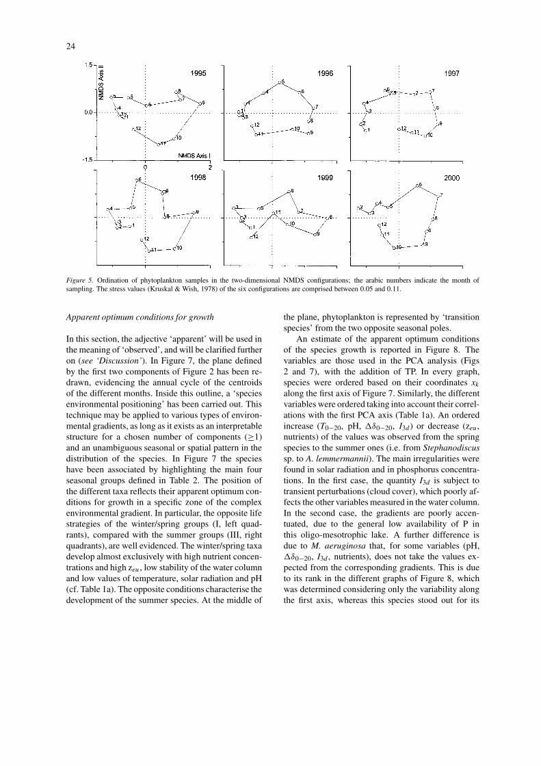
Figure 5. Ordination of phytoplankton samples in the two-dimensional NMDS configurations; the arabic numbers indicate the month ofsampling. The stress values (Kruskal & Wish, 1978) of the six configurations are comprised between 0.05 and 0.11.

Apparent optimum conditions for growth

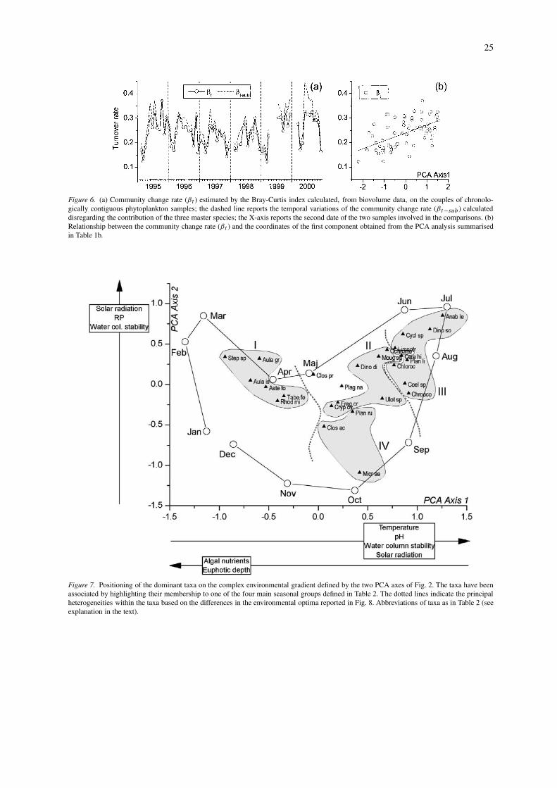
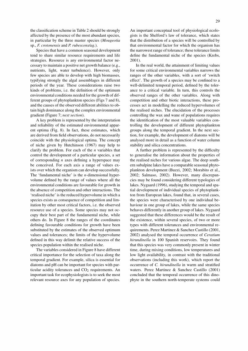
In this section, the adjective ‘apparent’ will be used inthe meaning of ‘observed’, and will be clarified furtheron (see ‘Discussion’). In Figure 7, the plane definedby the first two components of Figure 2 has been re-drawn, evidencing the annual cycle of the centroidsof the different months. Inside this outline, a ‘speciesenvironmental positioning’ has been carried out. Thistechnique may be applied to various types of environ-mental gradients, as long as it exists as an interpretablestructure for a chosen number of components (≥1)and an unambiguous seasonal or spatial pattern in thedistribution of the species. In Figure 7 the specieshave been associated by highlighting the main fourseasonal groups defined in Table 2. The position ofthe different taxa reflects their apparent optimum con-ditions for growth in a specific zone of the complexenvironmental gradient. In particular, the opposite lifestrategies of the winter/spring groups (I, left quad-rants), compared with the summer groups (III, rightquadrants), are well evidenced. The winter/spring taxadevelop almost exclusively with high nutrient concen-trations and high zeu, low stability of the water columnand low values of temperature, solar radiation and pH(cf. Table 1a). The opposite conditions characterise thedevelopment of the summer species. At the middle of

the plane, phytoplankton is represented by ‘transitionspecies’ from the two opposite seasonal poles.

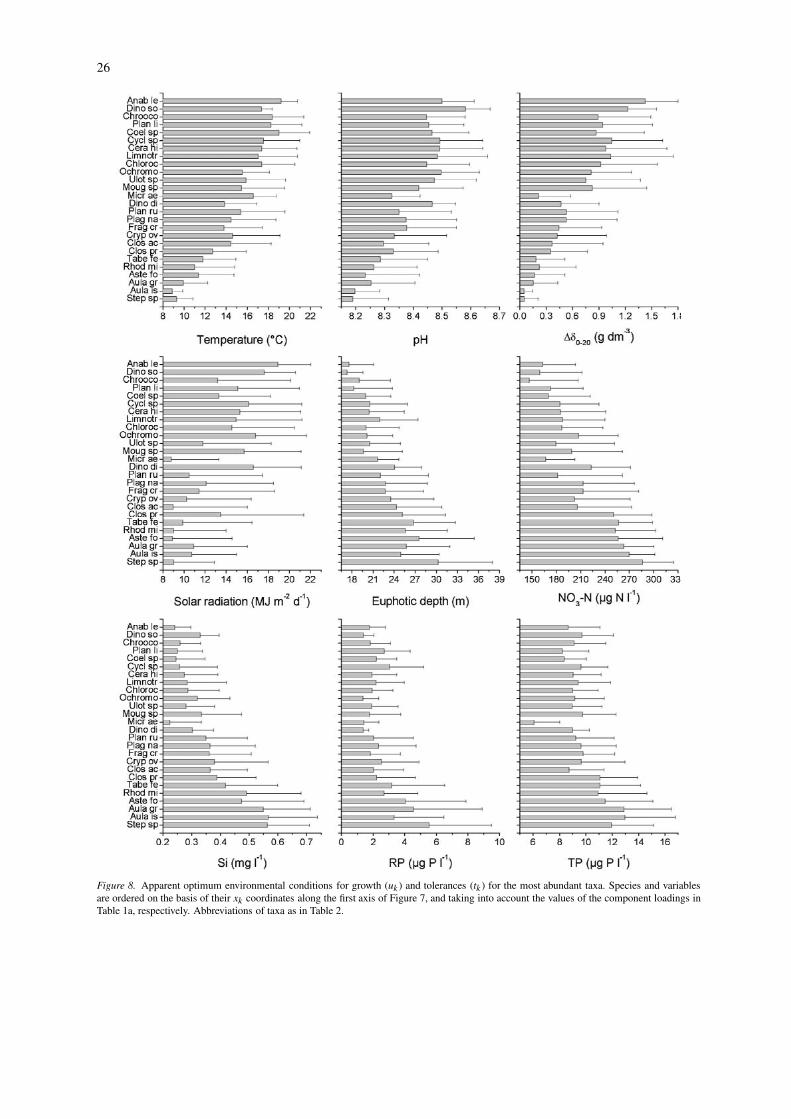
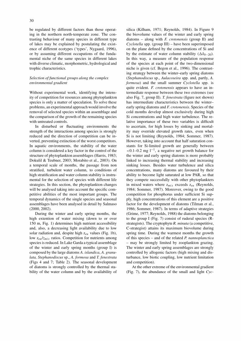
An estimate of the apparent optimum conditionsof the species growth is reported in Figure 8. Thevariables are those used in the PCA analysis (Figs2 and 7), with the addition of TP. In every graph,species were ordered based on their coordinates xk

along the first axis of Figure 7. Similarly, the differentvariables were ordered taking into account their correl-ations with the first PCA axis (Table 1a). An orderedincrease (T0−20, pH, �δ0−20, I3d) or decrease (zeu,nutrients) of the values was observed from the springspecies to the summer ones (i.e. from Stephanodiscussp. to A. lemmermannii). The main irregularities werefound in solar radiation and in phosphorus concentra-tions. In the first case, the quantity I3d is subject totransient perturbations (cloud cover), which poorly af-fects the other variables measured in the water column.In the second case, the gradients are poorly accen-tuated, due to the general low availability of P inthis oligo-mesotrophic lake. A further difference isdue to M. aeruginosa that, for some variables (pH,�δ0−20, I3d , nutrients), does not take the values ex-pected from the corresponding gradients. This is dueto its rank in the different graphs of Figure 8, whichwas determined considering only the variability alongthe first axis, whereas this species stood out for its

25

Figure 6. (a) Community change rate (βt ) estimated by the Bray-Curtis index calculated, from biovolume data, on the couples of chronolo-gically contiguous phytoplankton samples; the dashed line reports the temporal variations of the community change rate (βt−sub ) calculateddisregarding the contribution of the three master species; the X-axis reports the second date of the two samples involved in the comparisons. (b)Relationship between the community change rate (βt ) and the coordinates of the first component obtained from the PCA analysis summarisedin Table 1b.

Figure 7. Positioning of the dominant taxa on the complex environmental gradient defined by the two PCA axes of Fig. 2. The taxa have beenassociated by highlighting their membership to one of the four main seasonal groups defined in Table 2. The dotted lines indicate the principalheterogeneities within the taxa based on the differences in the environmental optima reported in Fig. 8. Abbreviations of taxa as in Table 2 (seeexplanation in the text).

26

Figure 8. Apparent optimum environmental conditions for growth (uk ) and tolerances (tk ) for the most abundant taxa. Species and variablesare ordered on the basis of their xk coordinates along the first axis of Figure 7, and taking into account the values of the component loadings inTable 1a, respectively. Abbreviations of taxa as in Table 2.

27

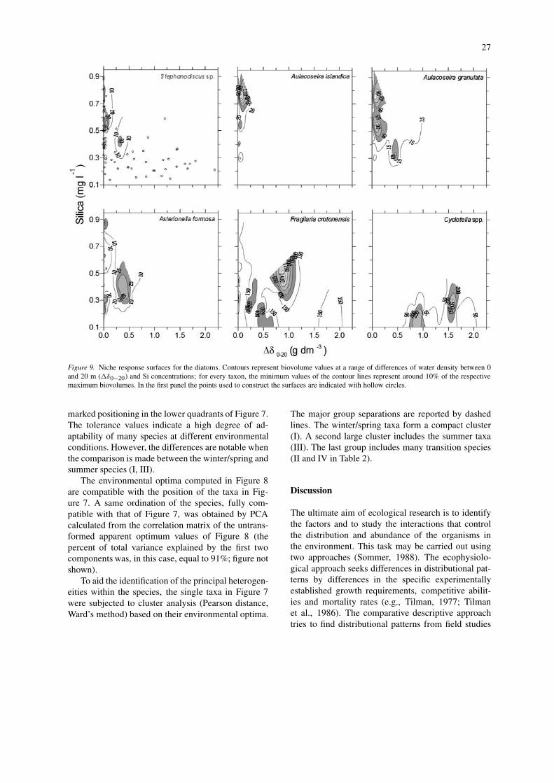
Figure 9. Niche response surfaces for the diatoms. Contours represent biovolume values at a range of differences of water density between 0and 20 m (�δ0−20) and Si concentrations; for every taxon, the minimum values of the contour lines represent around 10% of the respectivemaximum biovolumes. In the first panel the points used to construct the surfaces are indicated with hollow circles.

marked positioning in the lower quadrants of Figure 7.The tolerance values indicate a high degree of ad-aptability of many species at different environmentalconditions. However, the differences are notable whenthe comparison is made between the winter/spring andsummer species (I, III).

The environmental optima computed in Figure 8are compatible with the position of the taxa in Fig-ure 7. A same ordination of the species, fully com-patible with that of Figure 7, was obtained by PCAcalculated from the correlation matrix of the untrans-formed apparent optimum values of Figure 8 (thepercent of total variance explained by the first twocomponents was, in this case, equal to 91%; figure notshown).

To aid the identification of the principal heterogen-eities within the species, the single taxa in Figure 7were subjected to cluster analysis (Pearson distance,Ward’s method) based on their environmental optima.

The major group separations are reported by dashedlines. The winter/spring taxa form a compact cluster(I). A second large cluster includes the summer taxa(III). The last group includes many transition species(II and IV in Table 2).

Discussion

The ultimate aim of ecological research is to identifythe factors and to study the interactions that controlthe distribution and abundance of the organisms inthe environment. This task may be carried out usingtwo approaches (Sommer, 1988). The ecophysiolo-gical approach seeks differences in distributional pat-terns by differences in the specific experimentallyestablished growth requirements, competitive abilit-ies and mortality rates (e.g., Tilman, 1977; Tilmanet al., 1986). The comparative descriptive approachtries to find distributional patterns from field studies

28

and recorded abundances. This approach may fol-low different strategies (Gauch, 1982), whose choicedepends on the temporal and spatial scales involvedand on the life cycles of the studied organisms. Interrestrial vegetational studies, differences in the con-temporary composition and abundance may be fol-lowed along spatially extended habitats (e.g., alti-tudinal and moisture gradients; Whittaker, 1956) oralong temporal gradients, during primary successions(e.g., Wood & del Moral, 1987). With the comparat-ive approach, phytoplankton studies try to extrapolatespecific life traits from samplings carried out gener-ally with weekly or monthly frequency; eventually, thespecies that dominate the annual cycles from differentlakes ordinated along environmental gradients may becompared, to find their optimum conditions for growthfor a specific factor (e.g., trophic level or acidifica-tion; Reynolds, 1998; Lepistö, 1999). The study ofthe temporal changes in phytoplankton compositionand abundance (cf. Fig. 4) may be conceived as a dir-ect gradient analysis performed along a complex ofseasonally changing environmental variables. Thesevariables may present a high degree of correlation(e.g., Table 1a), acting jointly as a complex forcingfactor that selects seasonal groups of species sharingsimilar requirements. At the same time, it is not alwayseasy to extract the correct set of environmental vari-ates influencing the wax and wane of phytoplanktonfrom complex gradients. The intensity of competitionand the action of other biotic factors (e.g., grazing)occurring within the potential competitors at a par-ticular region of any complex environmental gradientdetermine the ultimate structure of the phytoplank-ton community, its diversity and seasonal dominancepatterns.

The complex environmental gradient

The whole set of environmental variables consideredin Figure 1 were characterised by a strong temporalcomponent. �δ0−20 values were highly correlatedwith the corresponding I3d values (r = 0.73; P < 0.01).Maximum average water temperatures in the layer 0–20 m were shifted of 1–2 months in comparison to theI3d maxima, with correlation coefficients equal to 0.73and 0.79 for time lags of 1 and 2 months, respectively,against an r value of 0.48 computed on the originaldata. The high degree of correlation of I3d and �δ0−20is reflected by their high loadings on the first two com-ponents (Table 1). The remaining variables (excludingRP), were strongly correlated only with the first com-

ponent, reflecting the existence of temporal lags alsoin the response of these variates against the increase ofsolar radiation.

The seasonal increase of pH values was stronglyassociated to phytoplankton activity. Salmaso & De-cet (1998) showed that, in Lake Garda, from 1995to 1996, H2CO3

∗ (CO2(aq) + H2CO3) concentrationsin the layer 0–20 m exceeded the equilibrium val-ues 1.5–2.5 fold from November to April. During thewarmest months (particularly June–August), a slightundersaturation (by 0.8–0.5 fold) was observed only atthe surface, whereas at 20 m H2CO3

∗ concentrationsremained around or a little above the air equilibriumvalues, suggesting the presence of only a partial lim-itation of the dissolved carbon on the phytoplanktongrowth in the layer 0–20 m for pH values rangingfrom 8.0 to 8.8. A computation of CO2 saturations onthe data from 1997 to 2000 essentially confirms theseconclusions.

The decrease of nutrients in the first 20 m beganafter the maximum spring replenishment, and in co-incidence with the stabilisation of the water column.Water flux from rivers is low, and mainly limited tothe northern shore of the lake, so that the spring sup-ply from the deep waters constitutes a significant inputof new nutrients to the productive layers every year.With the progressive formation of a stable and isolatedepilimnion (Fig. 1b,c), nutrients originating from thehypolimnetic waters decrease their importance, there-fore the phytoplankton growth from May to Septemberappears to rely also on nutrients regenerated by micro-bial mineralisation and zooplankton grazing (Salmaso& Decet, 1998).

The high regularity (Fig. 1) and high temporalsynchronicity (cf. Table 1a) that characterise the en-vironmental variables is due to a mix of causes likethe annual climatic evolution, the vertical mixing ofthe water column from late autumn to early spring (a‘homogenisation factor’), and the high inertial charac-teristics of this large system, which is able to minimiselocal perturbations (e.g., meteorological events), sothat the lake clearly bears the signs of the modifica-tions brought about by phytoplankton during summer.

Phytoplankton niches

The arrangement of the seasonal groups in Table 2aims to identify the most probable temporal locationof each species, leaving the differences in absoluteabundance with the other taxa out of consideration. Infact, if absolute biovolumes are used (Salmaso, 2002),

29

the classification scheme in Table 2 should be stronglyaffected by the presence of the most abundant species,in particular by the three master species (Mougeotiasp., F. crotonensis and P. rubescens/ag.).

Species that have a common seasonal developmenttend to share similar resource requirements and lifestrategies. Resource is any environmental factor ne-cessary to maintain a positive net growth balance (e.g.,nutrients, light, water turbulence). However, onlyfew species are able to develop with high biomasses,typifying strongly the algal assemblages in differentperiods of the year. These considerations raise twokinds of problems, i.e. the definition of the optimumenvironmental conditions needed for the growth of dif-ferent groups of phytoplankton species (Figs 7 and 8),and the causes of the observed different abilities to ob-tain high dominance along the complex environmentalgradient (Figure 7; next section).

A key problem is represented by the interpretationand reliability of the estimated environmental appar-ent optima (Fig. 8). In fact, these estimates, whichare derived from field observations, do not necessarilycoincide with the physiological optima. The conceptof niche given by Hutchinson (1967) may help toclarify the problem. For each of the n variables thatcontrol the development of a particular species, a setof corresponding n axes defining a hyperspace maybe conceived. For each axis a range of values ex-ists over which the organism can develop successfully.The ‘fundamental niche’ is the n-dimensional hyper-volume defined by the range of values where all theenvironmental conditions are favourable for growth inthe absence of competition and other interactions. The‘realised niche’ is the reduced hypervolume in which aspecies exists as consequence of competition and lim-itation by other most critical factors, i.e. the observedresource use of a species. Some species may not oc-cupy their best part of the fundamental niche, whileothers do. In Figure 8 the ranges of the coordinatesdefining favourable conditions for growth have beensubstituted by the estimates of the observed optimumvalues and tolerances; the limits of the hypervolumedefined in this way delimit the relative success of thespecies population within the realised niche.

The variables considered in Figure 8 have differentcritical importance for the selection of taxa along thetemporal gradient. For example, silica is essential fordiatoms and pH can be important for species with par-ticular acidity tolerances and CO2 requirements. Animportant task for ecophysiologists is to seek the mostrelevant resource axes for any population of species.

An important conceptual tool of physiological ecolo-gists is the Shelford’s law of tolerance, which statesthat the distribution of a species will be controlled bythat environmental factor for which the organism hasthe narrowest range of tolerance; these tolerance limitsdefine the fundamental niche of the species (Krebs,2001).

In the real world, the attainment of limiting valuesfor some critical environmental variables narrows theranges of the other variables, with a sort of ‘switcheffect’. The growth of a species may be confined to awell-delimited temporal period, defined by the toler-ance to a critical variable. In turn, this controls theobserved ranges of the other variables. Along withcompetition and other biotic interactions, these pro-cesses act in modelling the reduced hypervolumes ofthe realised niches. The elucidation of the processescontrolling the wax and wane of populations requiresthe identification of the most valuable variables con-trolling the development of different phytoplanktongroups along the temporal gradient. In the next sec-tion, for example, the development of diatoms will beanalysed more in detail as a function of water columnstability and silica concentrations.

A further problem is represented by the difficultyto generalise the information about the properties ofthe realised niches for various algae. The deep south-ern subalpine lakes have a comparable seasonal phyto-plankton development (Buzzi, 2002; Morabito et al.,2002; Salmaso, 2002). However, many discrepan-cies may be found considering different typologies oflakes. Nygaard (1996), studying the temporal and spa-tial development of individual species of phytoplank-ton from European lakes, found that, in several cases,the species were characterised by one individual be-haviour in one group of lakes, while the same speciesbehaves differently in another group of lakes. Nygaardsuggested that these differences would be the result ofthe existence, within several species, of two or moretypes with different tolerances and environmental re-quirements. Perez Martinez & Sanchez Castillo (2001,2002) analysed the temporal occurrence of Ceratiumhirundinella in 100 Spanish reservoirs. They foundthat this species was very commonly present in wintertime, during mixing conditions, low temperatures andlow light availability, in contrast with the traditionalobservations (including this work), which report theoccurrence of C. hirundinella in warm and stratifiedwaters. Perez Martinez & Sanchez Castillo (2001)concluded that the temporal occurrence of this dino-phyte in the southern north-temperate systems could

30

be regulated by different factors than those operat-ing in the northern north-temperate zone. The con-trasting behaviour of many species in different typeof lakes may be explained by postulating the exist-ence of different ecotypes (‘types’, Nygaard, 1996),or by assuming different occupations of the funda-mental niche of the same species in different lakeswith diverse climatic, morphometric, hydrological andtrophic characteristics.

Selection of functional groups along the complexenvironmental gradient

Without experimental work, identifying the intens-ity of competition for resources among phytoplanktonspecies is only a matter of speculation. To solve theseproblems, an experimental approach would involve theremoval of selected species within an assemblage andthe comparison of the growth of the remaining specieswith untreated controls.

In disturbed or fluctuating environments thestrength of the interactions among species is stronglyreduced and the direction of competition can be in-verted, preventing extinction of the worst competitors.In aquatic environments, the stability of the watercolumn is considered a key factor in the control of thestructure of phytoplankton assemblages (Harris, 1983;Dokulil & Teubner, 2003; Morabito et al., 2003). Ona temporal scale of months, the passage from nonstratified, turbulent water column, to conditions ofhigh stratification and water column stability is instru-mental for the selection of species with different lifestrategies. In this section, the phytoplankton changeswill be analysed taking into account the specific com-petitive abilities of the most important groups. Thetemporal dynamics of the single species and seasonalassemblages have been analysed in detail by Salmaso(2000, 2002).

During the winter and early spring months, thehigh extention of water mixing (down to or over150 m, Fig. 1) determines high nutrient accessibilityand, also, a decreasing light availability due to lowsolar radiation and, despite high zeu values (Fig. 1b),low zeu/zmix ratios. Competition for nutrients amongspecies is reduced. In Lake Garda a typical assemblageof the winter and early spring months (group I) iscomposed by the large diatoms A. islandica, A. granu-lata, Stephanodiscus sp., A. formosa and T. fenestrata(Figs 4 and 7; Table 2). The seasonal developmentof diatoms is strongly controlled by the thermal sta-bility of the water column and by the availability of

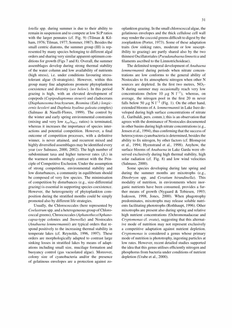
silica (Kilham, 1971; Reynolds, 1984). In Figure 9the biovolume values of the winter and early springdiatoms – along with F. crotonensis (group II) andCyclotella spp. (group III) – have been superimposedon the plane defined by the concentrations of Si andby the estimate of water column stability (�δ0−20).In this way, a measure of the population responseof the species at each point of the two-dimensionalniche is given (cf. Begon et al., 1996). The contrast-ing strategy between the winter–early spring diatoms(Stephanodiscus sp., Aulacoseira spp. and, partly, A.formosa) and the small summer Cyclotella spp. isquite evident. F. crotonensis appears to have an in-termediate response between these two extremes (seealso Fig. 7, group II). T. fenestrata (figure not shown)has intermediate characteristics between the winter–early spring diatoms and F. crotonensis. Species of thecold months develop almost exclusively during highSi concentrations and high water turbulence. The re-lative importance of these two variables is difficultto ascertain, for high losses by sinking and mortal-ity may override elevated growth rates, even whenSi is not limiting (Reynolds, 1984; Sommer, 1987).However, taking into account that half saturation con-stants for Si-limited growth are generally between<0.1–0.2 mg l−1, a negative net growth balance forthe winter and early spring diatoms is more probablylinked to increasing thermal stability and increasingsinking losses. Besides water turbulence and silicaconcentrations, many diatoms are favoured by theirability to become light saturated at low PAR, so thatthey compete successfully with other phytoplanktersin mixed waters where zmix exceeds zeu (Reynolds,1984; Sommer, 1987). Moreover, owing to the goodcompetition for phosphorus under sufficient Si sup-ply, high concentrations of this element are a positivefactor for the development of diatoms (Tilman et al.,1986; Sommer, 1987). In terms of adaptive strategies(Grime, 1977; Reynolds, 1988) the diatoms belongingto the group I (Fig. 7) consist of ruderal species (R-strategists). The cryptophyte R. minuta (a competitive,C-strategist) attains its maximum biovolume duringspring time. During the warmest months the growthof this species – and of the related P. nannoplanctica– may be strongly limited by zooplankton grazing.The winter and early spring assemblages are stronglycontrolled by allogenic factors (high mixing and dis-turbance, low biotic coupling, low nutrient limitationand competition).

At the other extreme of the environmental gradient(Fig. 7), the abundance of the small and light Cyc-

31

lotella spp. during summer is due to their ability toremain in suspension and to compete at low Si:P ratioswith the larger pennates (cf. Fig. 9) (Tilman & Kil-ham, 1976; Tilman, 1977; Sommer, 1987). Besides thesmall centric diatoms, the summer group (III) is rep-resented by many species belonging to different algalorders and sharing very similar apparent optimum con-ditions for growth (Figs 7 and 8). Overall, the summerassemblages develop during strong thermal stabilityof the water column and low availability of nutrients(high stress), i.e. under conditions favouring stress-tolerant algae (S-strategists). However, within thisgroup many fine adaptations promote phytoplanktoncoexistence and diversity (see below). In this periodgrazing is high, with an elevated development ofcopepods (Copipodiaptomus steueri) and cladocerans(Diaphanosoma brachyurum, Bosmina (Eub.) longic-ornis kessleri and Daphnia hyalina-galeata complex)(Salmaso & Naselli-Flores, 1999). The control bythe winter and early spring environmental constraints(mixing and very low zeu/zmix ratios) is terminated,whereas it increases the importance of species inter-actions and potential competition. However, a finaloutcome of competition processes, with a definitivewinner, is never attained, and recurrent mixed andhighly diversified assemblages may be identified everyyear (see Salmaso, 2000, 2002). The high number ofsubdominant taxa and higher turnover rates (βt ) inthe warmest months strongly contrast with the Prin-ciple of Competitive Exclusion. Under the assumptionof strong competition, environmental stability andlow disturbances, a community in equilibrium shouldbe composed of very few species. The minimisationof competition by disturbances (e.g., size-differentialgrazing) is essential in supporting species coexistence.However, the heterogeneity of phytoplankton com-position during the stratified months could be simplypromoted also by different life strategies.

Usually, the Chlorococcales (here represented byCoelastrum spp. and a heterogeneous group of Chloro-coccal greens), Chroococcales (Aphanothece/Aphano-capsa-type colonies and Snowella) and Nostocales(Anabaena lemmermannii) are typical orders that re-spond positively to the increasing thermal stability intemperate lakes (cf. Reynolds, 1996, 1997). Theseorders are morphologically adapted to contrast largesinking losses in stratified lakes by means of adapt-ations including small size, mucilage formation andbuoyancy control (gas vacuolated algae). Moreover,colony size of cyanobacteria and/or the presenceof gelatinous envelopes are a protection against zo-

oplankton grazing. In the small chlorococcal algae, thegelatinous envelopes and the thick cellulose cell wallmay render the coccoid greens difficult to digest by thezooplankton (Porter, 1973). Some of these adaptationtraits (low sinking rates, moderate or low suscept-ibility to grazing) are partly shared also by the twothinnest Oscillatoriales (Pseudanabaena limnetica andfilaments ascribed to the Limnotrichoideae).

The delimited temporal development of Anabaenalemmermannii during periods when nitrate concen-trations are low conforms to the general ability ofNostocales to fix atmospheric nitrogen when other Nsources are depleted. In the first two metres, NO3-N during summer may occasionally reach very lowconcentrations (below 10 µg N l−1), whereas, onaverage, the nitrogen pool in the first 20 m neverfalls below 50 µg N l−1 (Fig. 1). On the other hand,extended blooms of A. lemmermannii in Lake Iseo de-veloped during high surface concentrations of nitrate(L. Garibaldi, pers. comm.); this is an observation thatagrees with the dominance of Nostocales documentedin other basins during high nitrate concentrations (e.g.,Jensen et al., 1994), thus confirming that the success ofheterocystous cyanobacteria is determined, besides theability to fix nitrogen, by other factors (cf. Blomqvistet al., 1994; Hyenstrand et al., 1998). Anyhow, thesurface blooms of Anabaena in Lake Garda were ob-served exclusively during high thermal stability, highsolar radiation (cf. Fig. 8) and low wind velocities(Salmaso, 2000).

Some species developing during late spring andduring the summer months are mixotrophs (e.g.,Dinobryon spp. and Ceratium hirundinella). Thismodality of nutrition, in environments where inor-ganic nutrients have been consumed, provides a fur-ther means of growth (Nygaard & Tobiesen, 1993;Isaksson, 1998, Jones, 2000). When phagotrophypredominates, mixotrophs may release soluble nutri-ents facilitating phototrophs (Rothhaupt, 1996). Othermixotrophs are present also during spring and relativehigh nutrient concentrations (Ochromonadaceae andCryptomonas cf. ovata), suggesting that this alternat-ive mode of nutrition may not represent exclusivelya competitive adaptation against nutrient depletion.Cryptomonas is considered a genus whose primarymode of nutrition is phototrophy, ingesting particles atlow rates. However, recent detailed studies supportedthe idea that this genus utilises efficiently nitrogen andphosphorus from bacteria under conditions of nutrientdepletion (Urabe et al., 2000).

32

An additional strategy to supplement nutrients inphytoplankton may involve luxury uptake of N- andP-compounds (Reynolds, 1984). Nutrients may beaccumulated within cells as storage products depos-ited when their concentrations become high, e.g., inmicropatches from zooplankton excretion. P and Nlimitations are considered episodic in time and usu-ally weak. However, Hudson et al. (2000), using newradio-bioassay techniques, found that phosphate levelsin many lakes were two to three orders of magnitudelower than previously thought; this suggests that phos-phorus is the most essential of nutrients and so the staffof life (Karl, 2000).

These different ways to obtain nutrients reducethe competition among species (see also Steinberg &Geller, 1993). A further way to promote coexistenceis vertical migration. Phytoplankton during thermalstratification may be irregularly distributed in the eu-photic layer. For example, Anabaena lemmermanniiin Lake Garda forms wide surface patches with di-urnal dynamics, whereas Oscillatoriales sometimesdevelop metalimnetic maxima (Salmaso, 2000). Un-homogeneities in the phytoplankton distribution alongthe water column guarantee a major niche diversi-fication through the exploitation of different environ-mental gradients (cf. Levin, 1974). The positioning indifferent places in a given habitat to reduce competi-tion is a common strategy in nature. For instance, ina classic study, MacArthur (1958) explained the birddiversity in boreal forests by differences in their feed-ing positions on the tree branches and by differencesin food. The development of many fine evolutionaryadaptations, which favour niche differentiation and α

diversity, is a general characteristic of many plant andanimal communities (Wilson, 1992).

The different life strategies and biology of the com-ponent species described above contribute to increasethe diversity by means of endogenous mechanisms. Ingeneral, the organisation of the species through nicheand habitat partitioning tends to shape the communit-ies around their local equilibrium conditions.

Besides the above endogenous mechanisms, exo-genous factors can also promote diversity. Disturbanceeffects are considered as important promoters of com-munity diversity (Connell, 1978). A disturbance is anyepisode that changes the status of resources, disrupt-ing community structure and equilibrium dynamics.Several studies about the relationships between phyto-plankton diversity and disturbance have been made(Sommer et al., 1993; Reynolds et al., 1993). In largeand deep lakes characterised by low water renewal and

with algal production developing in a large euphoticlayer, physical disturbances are reduced in compar-ison to small systems (i.e. large and deep lakes havehigher stability and resilience, sensu Pimm, 1984).This finds support in the high regularities that char-acterise the development of the variables measuredin-lake in comparison to the higher variability of solarradiation. However, the existence of both endogen-ous and exogenous mechanisms promoting diversityis consistent with the view that real communities arespread along a continuum from equilibrium to non-equilibrium (Krebs, 2001). These mechanisms aretemporally scaled, providing a variety of ways inwhich the probability of coexistence is enhanced anddiversity increased (cf. Begon et al., 1996). From ageneral point of view, near-equilibrium communitiesare not necessarily destined to become dominated byvery few species.

The late spring/early summer species (group II)and the late summer/autumn species (group IV) haveapparent optimum conditions for growth at the middleof the environmental gradient (Table 2; Figs 7 and8). These two groups include several ruderal speciesdifferent from the filamentous centric diatoms. A fewof the species belonging to these intermediate groupsare adapted to develop within a wider range of envir-onmental conditions; in this case, however, the max-imum growth is attained in different periods (Table 2;Fig. 4). This is evident for the three master speciesMougeotia sp., Fragilaria crotonensis and Plankto-thrix rubescens/agardhii. High biovolume levels ofthese three taxa were not reached during periods char-acterised by high physical disturbance (deep mixingand low light) or during high thermal stratification,when equilibrium dynamics and competition are attheir seasonal maxima. The extreme physical controland the increase of competition for resources in oligo-trophic or mesotrophic lakes appear both incompatiblewith the attainment of high biovolume levels.

The factors causing the seasonal wax and wane ofthe three master species have been recently discussed(Salmaso, 2000, 2002). The dominance of Mougeotiasp. is promoted by its good competition for phos-phorus and its resistance against sinking (Padisák etal., 2003) and grazing. Laboratory experiments carriedout in Lake Constance showed that M. thylespora wasthe most successful competitor for P at low Si:P ratiosamong non diatoms; moreover, in-lake experimentscarried out in the field demonstrated that Mougeo-tia presented annual average sinking velocities in thelayer 0–20 m between 0.06–0.15 m d−1, against cor-

33

responding average velocities of 1.3–1.5 m d−1 foundfor the colonies of Fragilaria crotonensis (Sommer,1987). The large filaments of Mougeotia are poorlyedible by the zooplankton. A recent study carried outin Lake Garda on the susceptibility of phytoplanktonto grazing showed that the inedible unicellular frac-tion and filamentous algae became abundant duringthe maximum development of zooplankton, which iscoincident with the development of herbivorous clado-cerans (Salmaso, 2002). The collapse of this speciesduring the summer months takes place during thedeepening of mixing, decreasing zeu/zmix ratios andmaximum nutrient depletion.

In contrast with the large centric diatoms, thehigher development of F. crotonensis is limited tomoderate mixed conditions (Fig. 9). Its absence dur-ing the warmest months is due to high mortality byenhanced sinking and low Si availability.

Filaments of Planktothrix rubescens/agardhii areparticularly adapted to conditions of low irradiance(Reynolds, 1984), showing a vertical zonation dur-ing summer, with metalimnetic maxima around thelimit of the euphotic zone and vertical homogenisa-tion and dilution in autumn and winter (Salmaso,2000). Walsby et al. (1998) and Micheletti et al.(1998) showed that this seasonal evolution is linkedto the perennation strategy of Planktothrix in the deeplakes, with the autumn populations that survive in themixing column during the successive coldest months.Other two typical autumn species in Lake Garda areClosterium aciculare and Microcystis aeruginosa. Ap-parently, these two taxa appear to respond positively tomoderate water mixing and illumination.

Conclusions

The most abundant species living in the deep and largeLake Garda are characterised by regular annual de-velopments, which result from different selection ofspecific life traits along the complex environmentalgradient. The development of the different speciesduring their favourable growth period may be char-acterised by biovolume differences from year to year.However, at the community level, the temporal reg-ularities that distinguish the annual development ofphytoplankton are favoured by the high stability andresilience that characterise large and deep lakes withlow water renewal times.

The application of multivariate analyses basedon the different specific environmental optima high-

lighted the existence of three large algal groups. Thefirst was represented by the winter and early springdiatoms (Aulacoseira spp., Stephanodiscus spp., As-terionella formosa and Tabellaria fenestrata). Thisgroup develops during high water turbulence, highnutrient concentrations, low light conditions and lowzeu/zmix ratios. The competition is reduced and thecommunity is under strong physical control. At theopposite extreme of the complex environmental gradi-ent (summer months), the second group was composedby many species belonging to cyanobacteria (thin Os-cillatoriales, Nostocales and Chroococcales), Chloro-coccales and coccal greens, Dinobryon sociale andCeratium hirundinella. Common life history traits inthis group include the ability to contrast losses bygrazing and sinking in stratified and stable conditions,and the ability to tolerate nutrient deficiency. The re-maining group developed in the ‘intermediate’ seasons(mainly late spring/early summer and/or autumn), i.e.during environmental conditions (and, possibly, stresscompetition) in the middle of the two previous ex-tremes. This group is strongly typified by the threemaster species Mougeotia sp., F. crotonensis and P.rubescens/ag.. These taxa are characterised by higherbiovolumes and extended periods of dominance incomparison to the remaining subdominants. Their suc-cess appears favoured by different abilities to contrastgrazing and sinking. High dominance of the three mas-ter species is prevented during high physical disturb-ance (mixing and low light) or during high stabilityof the water column, when equilibrium dynamics andcompetition are at their seasonal maximum.

During the summer months, the increasing thermalstability of the water column coincides with the max-imum nutrient depletion; compared with the groupsdeveloping during mixing and higher nutrient con-centrations, the interaction and competition amongspecies increase, but without the selection of exclusivewinners. In contrast with the Principle of CompetitiveExclusion, the elevated number of coexisting speciesdoes not find support with equilibrium dynamics con-trolled by competition. Many factors, regulated byphytoplankton or under external control, can minimisecompetition, allowing the coexistence of many phyto-plankton species in stratified and stable environments.Exogenous factors are represented by disturbanceevents which tend to disrupt equilibrium dynamics.Endogenous factors consist of many fine adaptations,which include vertical positioning, supplemented as-similation of nutrients by mixotrophy, N-fixation byNostocales and luxury consumption; these factors tend

34

to shape the community around its local equilibrium,by means of niche and habitat partitioning. The overallbalance is consistent with the existence of a phyto-plankton community oscillating along a continuum,from equilibrium to non-equilibrium. Anyhow, theenhancement of competition among species with sim-ilar requirements and the coexistence of different lifestrategies, has the property to increase the communitychange rate, which, during the stratified period, is atits maximum.

The disturbances acting on short to medium timeand the existence of fine adaptations reducing com-petition increase α diversity. These factors, whichact with different intensity over the seasons, mayalso contribute to the temporal differentiation of algalassemblages. On the other side, besides the abovefactors, βt diversity in medium and high latitude re-gions is strongly promoted by slow and regular annualevolution of the climatic variables. Under these as-sumptions, a hypothetical attainment of equilibriumconditions in phytoplankton communities could beonly transient (locally stable equilibrium). Equilib-rium communities tend to be stable (sensu Pimm,1984), recovering quickly from disturbances and withhigh persistence over time. However, time changesthe rules of the game continually, interfering withthe competitive exclusion dynamics. Over a temporalscale of years, phytoplankton undergo cyclic compos-itional changes which are comparable, as magnitude,to those that may be documented in terrestrial veget-ation over the millennia during the glacial-interglacialcycles (e.g., Miyoshi et al., 1999). In these two cases,the identification of equilibrium conditions strictlydepends on the choice of the temporal window. Ifscaled over many generations, vegetation communit-ies never approach stable and continuous equilibriumconditions.

For every phytoplankton species, the estimates ofthe optimum conditions for growth and the realisedniches must be considered mostly specific for this pe-culiar type of lake. The potential colonising capacity,survival and high reproductive growth of a particularspecies in response to the most relevant environmentalaxes (defined by its fundamental niche) is strongly re-duced both by environmental constraints typical of thecharacteristics of the colonised lakes, and by compet-ition dynamics. More abiotic and biotic factors mustbe considered in the study of species distribution indifferent types of lakes. Many discrepancies and thelack of unifying concepts in the studies regarding thedistribution of phytoplankton along trophic gradients

originated from the implicit reductive assumption ofthe existence of selective factors acting almost exclus-ively along a unique environmental axis. In particular,the significance of the morphometric, hydrologicaland climatic characteristics of lakes as selective factorshave been largely overlooked.

Acknowledgements

I am grateful to Prof. Ireneo Ferrari and Prof. PierluigiViaroli (Dipartimento di Scienze Ambientali, Uni-versità di Parma) for their hepful comments on anearlier version of this work. The manuscript receivedhelpful suggestions from two anonymous referees. Iam grateful to Dr Rosario Mosello (CNR-Istituto perlo Studio degli Ecosistemi, Pallanza) for motivatingdiscussions on the limnology of the deep southern sub-alpine lakes. I wish to thank Prof. Paolo Cordella (Di-partimento di Biologia, Università di Padova), Dr Fa-bio Decet (ARPAV-Belluno) and Dr Giorgio Franzini(ARPAV-Verona) for critical discussions and logisticsupport. This work was partially funded by the Ven-eto Region and ARPAV (Veneto Region EnvironmentProtection Agency).

References

Anagnostidis, K. & J. Komárek, 1988. Modern approach to theclassification system of Cyanophytes. 3-Oscillatoriales. Archivfür Hydrobiol./Algol. Stud. 50–53: 327–472.

APHA, AWWA & WEF., 1989. Standard methods for the examina-tion of water and wastewater. 17th edn, American Public HealthAssociation, Washington.

Begon, M., J. L. Harper, C. R. Townsend, 1996. Ecology. Individu-als, populations and communities. 3rd edn, Blackwell ScienceLtd, Oxford. 1068 pp.

Bleiker, W. & F. Schanz, 1987. Influence of environmental factorson the phytoplankton spring bloom in Lake Zürich. Aquat. Sci.51: 47–58.

Blomqvist, P., A. Petterson & P. Hyenstrand, 1994. Ammonium-nitrogen: a key regulatory factor causing dominance of non-nitrogen-fixing cyanobacteria in aquatic systems. Archiv fürHydrobiol. 132: 141–164.

Bondarenko, N. A., N. E. Guselnikova, N. F. Logacheva & G. V.Pomazkina, 1996. Spatial distribution of phytoplankton in LakeBaikal, spring 1991. Freshwat. Biol. 35: 517–523.

Bray, J. R. & J. T. Curtis, 1957. An ordination of the uplandforest communities of Southern Wisconsin. Ecol. Monogr. 27:325–349.

Buzzi, F., 2002. Phytoplankton assemblages in two sub-basins ofLake Como. J. Limnol. 61: 117–128.

Chen, C. T. & F. J. Millero, 1986. Precise thermodynamic propertiesfor natural waters covering only the limnological range. Limnol.Oceanogr. 31: 657–662.

35

Connell, J. H., 1978. Diversity in tropical rain forests and coralreefs. Science 199: 1302–1310.

Decet, F. & N. Salmaso, 1997. Indagini preliminari sulle caratter-istiche chimiche dei principali affluenti e dell’emissario del Lagodi Garda. Acqua Aria 7: 91–97.

Dokulil, M. T. & K. Teubner, 2003. Steady state phytoplankton as-semblages during thermal stratification in deep alpine lakes. Dothey occur? Hydrobiologia 502 (Dev. Hydrobiol. 172): 65–72.

Fabbro, L. D. & L. J. Duivenvoorden, 2000. A two-part modellinking multidimensional environmental gradients and seasonalsuccession of phytoplankton assemblages. Hydrobiologia 438:13–24.

Field, J. G., K. R. Clarke & R. M. Warwick, 1982. A practicalstrategy for analysing multispecies distribution patterns. Mar.Ecol. Prog. Ser. 8: 37–52.

Gauch, H. G., 1982. Multivariate analysis in community ecology.Cambridge University Press, Cambridge. 298 pp.

Grime, J. P., 1977. Evidence for the existence of three primarystrategies in plants and its relevance to ecological and evolution-ary theory. The American Naturalist 111: 1169–1194.

Hardin, G., 1960. The competitive exclusion principle. Science 131:1292–1297.

Harris, G. P., 1983. Mixed layer physics and phytoplankton popula-tions: studies in equilibrium and non-equilibrium ecology. Prog.Phycol. Res. 2: 1–52.

Hudson, J. J., W. D. Taylor & D. W. Schindler, 2000. Phosphateconcentrations in lakes. Nature 406: 54–56.

Hutchinson, G. E., 1961. The paradox of the plankton. Am. Nat. 95:137–145.

Hutchinson, G. E., 1967. A treatise on limnology, 2. Wiley & Sons,New York. 1115 pp.

Hyenstrand, P., P. Blomqvist & A. Petterson, 1998. Factors de-termining cyanobacterial success in aquatic systems – a literaturereview. Archiv für Hydrobiol./Adv. Limnol. 51: 41–62.

IRSA, 1974. Indagini sul Lago di Garda. IRSA Quaderni 18, Roma.540 pp.

Isaksson, A. 1998. Phagotrophic phytoflagellates in lakes – aliterature review. Archiv für Hydrobiol./Adv. Limnol. 51: 63–90.

Jensen, J. P., E. Jeppesen, K. Olrik & P. Kristensen, 1994. Impactof nutrients and physical factors on the shift from cyanobacterialto chlorophyte dominance in shallow Danish lakes. Can. J. Fish.aquat. Sci. 51: 1692–1699.

Jones, R. I., 2000. Mixotrophy in planktonic protists: an overview.Freshwat. Biol. 45: 219–226.

Karl, D. M., 2000. Phosphorus, the staff of life. Nature 406: 31–33.Kilham, P., 1971. A hypothesis concerning silica and the freshwater

plankton diatoms. Limnol. Oceanogr. 16: 10–18.Krebs, C. J., 2001. Ecology. 5th edn, Addison-Wesley, San Fran-

cisco. 695 pp.Kruskal, J. B. & M. Wish, 1978. Multidimensional scaling. Sage

Publications, Beverly Hills and London. 93 pp.Lepistö, L., 1999. Phytoplankton assemblages reflecting the ecolo-

gical status of lakes in Finland. Monogr. Boreal Environ. Res. 16.43 pp.

Levin, S. A., 1974. Dispersion and population interactions. Am.Nat. 108: 207–228.

Lorenzen, C. J., 1967. Determination of Chlorophyll and Pheo-Pigments: spectrophotometric equations. Limnol. Oceanogr. 12:343–346.

Lund, J. W. G., C. Kipling, & E. D. Le Cren, 1958. The inverted mi-croscope method of estimating algal numbers and the statisticalbasis of estimations by counting. Hydrobiologia 11: 143–170.

MacArthur, R. H., 1958. Population ecology of some warblers ofnortheastern coniferous forests. Ecology 39: 599–619.

Magurran, A. E., 1988. Ecological diversity and its measurement.Croom Helm, London. 179 pp.

McCook, L. J., 1994. Understanding ecological community suc-cession: causal models and theories, a review. Vegetatio 110:115–147.

Micheletti, S., F. Schanz & A. E. Walsby, 1998. The daily integ-ral of photosynthesis by Planktothrix rubescens during summerstratification and autumnal mixing in Lake Zurich. New Phytol.139: 233–246.

Miyoshi, N., T. Fujiki & Y. Morita, 1999. Palynology of a 250-m core from Lake Biwa: a 430 000-year record of glacial-interglacial vegetation change in Japan. Rev. Palaeobot. Palynol.104: 267–283.

Morabito, G., A. Oggioni & P. Panzani, 2003. Phytoplankton as-semblage at equilibrium in large and deep subalpine lakes: a casestudy from Lago Maggiore (N. Italy). Hydrobiologia 502 (Dev.Hydrobiol. 172): 37–48.

Morabito, G., D. Ruggiu & P. Panzani, 2002. Recent dynamics(1995-1999) of the phytoplankton assemblages in Lago Mag-giore as a basic tool for defining association patterns in the Italiandeep lakes. J. Limnol. 61: 129–145.

Novarino, G., I. A. N. Lucas & S. Morrall, 1994. Observa-tions on the genus Plagioselmis (Cryptophyceae). Cryptogamie,Algologie 15: 87–107.

Nygaard, G., 1996. Temporal and spatial development of individualspecies of plankton algae from European lakes. Hydrobiologia332: 71–91.

Nygaard, K. & A. Tobiesen, 1993. Bacterivory in algae: a survivalstrategy during nutrient limitation. Limnol. Oceanogr. 38: 273–279.

Padisák, J., 1994. Identification of relevant time-scales in non-equilibrium community dynamics: conclusions from phyto-plankton surveys. New Zealand J. Ecol. 18: 169–176.

Padisák. J., É. Soróczki-Pintér & Zs. Rezner, 2003. Sinking proper-ties of some phytoplankton shapes and the relation of form res-istance to morphological diversity of plankton: an experimentalstudy. Hydrobiologia 500: 243–257.

Perez Martinez, C. & P. Sanchez Castillo, 2001. Temporal occur-rence of Ceratium hirundinella in Spanish reservoirs. Hydrobio-logia 452: 101–107.

Perez Martinez, C. & P. Sanchez Castillo, 2002. Winter dominanceof Ceratium hirundinella in a southern north-temperate reservoir.J. Plankton Res. 24: 89–96.

Pimm, S. L., 1984. The complexity and stability of ecosystems.Nature 307: 321–326.

Porter, K. G., 1973. Selective grazing and differential digestion ofalgae by zooplankton. Nature 244: 179–180.

Reynolds, C. S., 1984. The ecology of freshwater phytoplankton.Cambridge University Press, Cambridge. 384 pp.

Reynolds, C. S., 1988. Functional morphology and the adaptivestrategies of freshwater phytoplankton. In Sandgren C. D. (ed.),Growth and Reproductive Strategies of Freshwater Phytoplank-ton. Cambridge University Press, Cambridge: 388–433.

Reynolds, C. S., 1996. The plant life of the pelagic. Int. Ver. theor.angewan. Limnol.: Verh. 26: 97–113.

Reynolds, C. S., 1997. Vegetation processes in the pelagic: a modelfor ecosystem theory. Ecology Institute, Oldendorf. 371 pp.

Reynolds, C. S., 1998. What factors influence the species com-position of phytoplankton in lakes of different trophic status?Hydrobiologia 369/370: 11–26.

Reynolds, C. S., J. Padisák & U. Sommer, 1993. Intermediate dis-turbance in the ecology of phytoplankton and the maintenance ofspecies diversity: a synthesis. Hydrobiologia 249: 183–188.

36

Rothhaupt, K. O., 1996. Laboratory experiments with a mixotrophicchrysophyte and obligately phagotrophic and phototrophic com-petitors. Ecology 77: 716–724.

Salmaso, N., 1996. Seasonal variation in the composition and rate ofchange of the phytoplankton community in a deep subalpine lake(Lake Garda, Northern Italy). An application of nonmetric mul-tidimensional scaling and cluster analysis. Hydrobiologia 337:49–68.

Salmaso, N., 2000. Factors affecting the seasonality and distributionof cyanobacteria and chlorophytes: a case study from the largelakes south of the Alps, with special reference to Lake Garda.Hydrobiologia 438: 43–63.

Salmaso, N., 2002. Ecological patterns of phytoplankton as-semblages in Lake Garda: seasonal, spatial and historical fea-tures. J. Limnol. 61: 95–115.

Salmaso, N. & F. Decet, 1997. Seasonal and interannual changes ofchemical characteristics and phytoplankton in a mountain lakeof the eastern Italian Alps (Lake Calaita, Trentino). Int. Rev. ges.Hydrobiol. 82: 15–31.

Salmaso, N. & F. Decet, 1998. Interactions of physical, chem-ical and biological processes affecting the seasonality of mineralcomposition and nutrient cycling in the water column of adeep subalpine lake (Lake Garda, Northern Italy). Archiv fürHydrobiol. 142: 385–414.

Salmaso, N. & L. Naselli-Flores, 1999. Stud. on the zooplankton ofthe deep subalpine Lake Garda. J. Limnol. 58: 66–76.

Salmaso, N., F. Decet, G. Franzini & P. Cordella. 2001. Evoluzionetrofica del Lago di Garda in relazione alla completa circolazionedelle acque del 1999 e 2000. Atti Ass. Ital. Oceanol. Limnol. 14:109–123.

Sommer, U., 1987. Factors controlling the seasonal variation inphytoplankton species composition. A case study for a deep,nutrient rich lake. Prog. Phycol. Res. 5: 123–178.

Sommer, U., 1988. Growth and survival strategies of planktonicdiatoms. In Sandgren, C. D. (ed.), Growth and ReproductiveStrategies of Freshwater Phytoplankton. Cambridge UniversityPress, Cambridge: 227–260.

Sommer, U., J. Padisák, C. S. Reynolds & P. Juhász-Nagy, 1993.Hutchinson’s heritage: the diversity-disturbance relationship inphytoplankton. Hydrobiologia 249: 1–7.

Steinberg, C. E. W. & W. Geller, 1993. Biodiversity and interactionswithin pelagic nutrient cycling and productivity. In Schulze, E.-D. & H. A. Mooney (eds), Biodiversity and Ecosystem Function.Ecological Studies 99: 43–64.

Ter Braak, C. J. F. & H. van Dam, 1989. Inferring pH from diatoms:a comparison of old and new calibration methods. Hydrobiologia178: 209–223.

Tilman, D., 1977. Resource competition between planktonic algae:an experimental and theoretical approach. Ecology 58: 338–348.

Tilman, D. & S. S. Kilham, 1976. Phosphate and silicate uptakeand growth kinetics of the diatoms Asterionella formosa andCyclotella meneghiniana in batch and semicontinuous culture.J. Phycol. 12: 375–383.

Tilman, D., R. Kiesling, R. Sterner, S. S. Kilham & F. Johnson,1986. Green, bluegreen and diatom algae: taxonomic differ-ences in competitive ability for phosphorus, silicon and nitrogen.Archiv für Hydrobiol. 106: 473–485.

Urabe, J., T. B. Gurung, T. Yoshida, T. Sekino, M. Nakanishi, M.Maruo & E. Nakayama, 2000. Diel changes in phagotrophy byCryptomonas in Lake Biwa. Limnol. Oceanogr. 45: 1558–1563.

Walsby, A. E., A. Avery & F. Schanz, 1998. The critical pressuresof gas vesicles in Planktothrix rubescens in relation to the depthof winter mixing in Lake Zurich, Switzerland. J. Plankton Res.20: 1357–1375.

Whittaker, R. H., 1956. Vegetation of the Great Smoky Mountains.Ecol. Monogr. 26: 1–80.

Whittaker, R. H., 1972. Evolution and measurement of speciesdiversity. Taxon 21: 213–251.

Wilkinson, L., 1990. SYGRAPH: The system for graphics. Evan-ston, IL, Systat, Inc.. 547 pp.

Wilson, E. O., 1992. The diversity of life. Penguin Books, London.406 pp.

Wood, D. M. & R. del Moral, 1987. Mechanisms of early primarysuccession in subaline habitats on Mount St. Helens. Ecology 68:780–790.