LCA FOR RENEWABLE RESOURCES

Ivan Muñoz & Karin Flury & Niels Jungbluth &

Giles Rigarlsford & Llorenç Milà i Canals & Henry King

Received: 3 August 2012 /Accepted: 11 June 2013 /Published online: 5 December 2013# Springer-Verlag Berlin Heidelberg 2013

AbstractPurpose Bio-based products are often considered sustainabledue to their renewable nature. However, the environmentalperformance of products needs to be assessed considering alife cycle perspective to get a complete picture of potentialbenefits and trade-offs. We present a life cycle assessment ofthe global commodity ethanol, produced from different feed-stock and geographical origin. The aim is to understand themain drivers for environmental impacts in the production ofbio-based ethanol as well as its relative performance comparedto a fossil-based alternative.Methods Ethanol production is assessed from cradle to gate;furthermore, end-of-life emissions are also included in order toallow a full comparison of greenhouse gas (GHG) emissions,assuming degradation of ethanol once emitted to air fromhousehold and personal care products. The functional unit is1 kg ethanol, produced frommaize grain in USA, maize stoverin USA, sugarcane in North-East of Brazil and Centre-South ofBrazil, and sugar beet and wheat in France. As a reference,ethanol produced from fossil ethylene in Western Europe is

used. Six impact categories from the ReCiPe assessment meth-od are considered, along with seven novel impact categories onbiodiversity and ecosystem services (BES).Results and discussion GHGemissions per kilogrambio-basedethanol range from 0.7 to 1.5 kg CO2 eq per kg ethanol and from1.3 to 2 kg per kg if emissions at end-of-life are included. Fossil-based ethanol involves GHG emissions of 1.3 kg CO2 eq per kgfrom cradle-to-gate and 3.7 kg CO2 eq per kg if end-of-life isincluded.Maize stover in USA and sugar beet in France have thelowest impact from a GHG perspective, although when otherimpact categories are considered trade-offs are encountered. BESimpact indicators show a clear preference for fossil-based etha-nol. The sensitivity analyses showed how certainmethodologicalchoices (allocation rules, land use change accounting, land usebiomes), as well as some scenario choices (sugarcane harvestmethod, maize drying) affect the environmental performance ofbio-based ethanol. Also, the uncertainty assessment showed thatresults for the bio-based alternatives often overlap, making itdifficult to tell whether they are significantly different.Conclusions Bio-based ethanol appears as a preferable optionfrom a GHG perspective, but when other impacts are consid-ered, especially those related to land use, fossil-based ethanolis preferable. A key methodological aspect that remains to beharmonised is the quantification of land use change, which hasan outstanding influence in the results, especially on GHGemissions.

Keywords Bioethanol . Bio-based . Biogenic feedstock .

LCA .Maize . Sugarcane . Sugar beet . Wheat

1 Introduction

There is a global trend to move away from a dependence on afossil fuel-based economy driven by such factors as combatingclimate change, the anticipation of rising prices for fossil fuelsand the desire of many countries to reduce external resource

Responsible editor: Sangwon Suh

Electronic supplementary material The online version of this article(doi:10.1007/s11367-013-0613-1) contains supplementary material,which is available to authorized users.

I. Muñoz :G. Rigarlsford (*) : L. M. i Canals :H. KingSafety and Environmental Assurance Centre, Unilever,Sharnbrook MK44 1LQ, UKe-mail: giles.rigarlsford@unilever.com

I. Muñoze-mail: ivan.munoz@unilever.com

K. Flury :N. JungbluthESU-services Ltd, Margrit Rainer-Strasse 11c, 8050 Zurich,Switzerland

I. Muñoz2.-0 LCA Consultants, Skibbrogade 5, 1, 9000 Aalborg, Denmark

Int J Life Cycle Assess (2014) 19:109–119DOI 10.1007/s11367-013-0613-1

Life cycle assessment of bio-based ethanol producedfrom different agricultural feedstocks

dependency (de Jong et al. 2012). Bio-based products are oftenconsidered preferable to fossil-based alternatives due to theirrenewable nature; however, the environmental profile of aproduct can be more complex than that, and hence a life cycleapproach is required to assess potential benefits as well astrade-offs (Miller et al. 2007). A typical example of a bio-based commodity chemical is ethanol, which is used mainly asa biofuel, but also as a solvent, raw material for chemicalproduction and for human consumption (Linak et al. 2009).Around 74,000 million litres of bioethanol were produced in2009, with USA and Brazil accounting for 88 % of the totalworld production (Biofuels Platform 2010). Ethanol is mainlyproduced by fermentation of sugars but it can also be producedsynthetically from petroleum, although the latter route is rap-idly declining relative to fermentation (Linak et al. 2009). Bio-based ethanol is currently produced using a variety of agricul-tural feedstocks such as maize, sugarcane, wheat, sugar beet,molasses, cassava as well as cellulosic biomass. Ethanol rep-resents an interesting example of a bio-based chemical that iscurrently produced in high volumes and with potentially quitedifferent environmental profiles, depending on the feedstockused and the region in the world where it is produced. To date,ethanol has been extensively investigated in life cycle assess-ment (LCA) studies, mainly from a transport bio-fuel perspec-tive (Fu et al. 2003; Nguyen and Gheewala 2008a, b; Omettoet al. 2009). However, very often the literature is focused onthe assessment of greenhouse gas (GHG) emissions only (Kimand Dale 2009; Silalertruksa and Gheewala 2011; Laborde2011; USEPA 2010), and most of the cited studies tend tofocus on a single agricultural feedstock for ethanol production.Recent work conducted under the UNEP/SETAC Life CycleInitiative has led to the development of novel methods toaccount for impacts of land use and land use change onbiodiversity and ecosystem services (BES) (Koellner et al.

2013). This is of the utmost importance in the context of bio-based products.

In this article, we present the results of an LCA study ofethanol production with different agricultural feedstock indifferent regions: maize grain and maize stover in the USA,sugarcane in two regions of Brazil and wheat and sugar beet inFrance. The aim of the study was to identify the main activitiesin the life cycle driving the various potential environmentalimpacts and to explore the differences between feedstocks, aswell as to benchmark bio-based ethanol with fossil-basedethanol from a cradle-to-grave perspective. The novelty ofthis work lies in the following aspects: it assesses ethanol asa feedstock for the chemical industry, rather than as biofuelwhich has been the focus of all studies to date; it consistentlyassesses a relatively high number of production routes; itincorporates a full set of novel impact categories focusing onBES; and thorough sensitivity and uncertainty analyses arecarried out to ensure the robustness of the results.

2 Methods

The approach taken in this case study is a descriptive(attributional) LCA and the functional unit is 1 kg of ethanolwith a water content of 5 %.

2.1 Investigated countries and biomass resources

The choice of feedstock and producing countries was basedon market research and production volumes, agriculturalpractices and on life cycle inventory data availability. Dueto their global importance, production from maize in theUSA and from sugarcane in Brazil was considered. Maizegrain and stover were assessed separately, and for sugarcane

Cultivation Ethanol production

Fertilisers, pesticides

Infrastructure

Waterconsumption

Background syste

m

Land use

Energy

Natural resources: sun, rain, wind, water, resources

ecoinvent processes

Waste water

Waste

Raw materials

ecoinvent processes

Water use

Land use

Energy

Material/chemicals

Waste water

Water use

Transport

Waste

Fore

ground system

Distribution, use (excluded)

Emissions to nature: air, water, soil

Ethanol disposal (released to air)

Fore

ground system

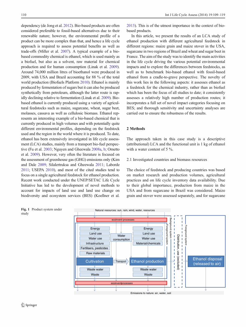
Fig. 1 Product system understudy

110 Int J Life Cycle Assess (2014) 19:109–119

two Brazilian regions were assessed due to climatic differ-ences: the North-East region and the Centre-South region.Wheat and sugar beet were assessed in France as it is animportant European ethanol-producing country.

2.2 System boundaries

Ethanol production from the considered feedstock was assessedfrom cradle-to-gate, as shown in Fig. 1. This includes cultivationof the feedstock, its transport to the mill and the processing toethanol. Furthermore, end-of-life emissions are included in orderto allow a full comparison of the GHG emissions associated withbio-based and fossil-based ethanol (see Section 2.6.5). All

remaining activities between the factory gate and disposal areexcluded, as these are common to all scenarios.

2.3 Allocation

When maize stover is harvested along with grain, maize culti-vation becomes a multi-output process, which was modelledby means of allocation based on economic value. Also, theprocessing of all feedstocks to ethanol results in other co-products, as shown in Table 1. Again, allocation based oneconomic value was performed. Even though the ISO stan-dards on LCA identify economic allocation as the last feasibleoption, the literature shows that it is one of the most common

Table 1 Key figures for the cultivation and processing of the different feedstocks under study (Flury and Jungbluth 2012)

Cultivation Unit Sugarcane,BR CS

Sugarcane,BR NE

Maize grain,US

Maize grainand stover, USa

Sugar beet,FR

Wheat,FR

Yield, main product kg/ha 82,697 57,677 9,703 9,703 84,649 6,605

Allocation % 81 % 100 %

Co-product Stover Straw

Yield, by-product kg/ha 4,676 0

Allocation % 19 % 0 %

Seed kg/ha 6,616 4,614 21 21 2 135

N-fertiliser kg/ha 76 31 157 167 103 150

P2O5 fertiliser kg N/ha 25 22 67 73 68 24

K2O fertiliser kg P2O5/ha 102 75 82 120 146 23

Lime kg/ha 305 213 366 366 0.1 12

Pesticides kg/ha 6 4 3 2.5 3 3

Diesel kg/ha 129 90 46 46 160 68

Land burned inpre-harvest

% 70 % 70 %

Land transformation ha/ha 0.032 0.032 0.016

Transport, total tkm/ha 2,771 1,933 479 479 1,432 338

Water consumption m3/ha 1,884 4,579 3,168 3,168 184 87

Processing Unit Sugarcane, BR CS Sugarcane, BR NE Maize grain, US Maize stover, USa Sugar beet, FR Wheat, FR

Feedstock input kg/kg ethanol 15.4 15.4 2.5 3.9 16.9 2.5

Chemicals kg/kg ethanol 0.03 0.03 0.02 0.21 0.43 0.02

Electricity kWh/kg ethanol 0.17 0.09 0.1

Heat MJ/kg ethanol 2.6 5.1

Transport tkm/kg ethanol 0.33 0.33 0.19 0.43 0.98 0.27

Water consumption L/kg ethanol −6.1 −6.1 −0.3 4.9 6.5 0.31

Allocation factors:

Ethanol % 50 % 50 % 84 % 87 % 89 % 73 %

Electricity % 8 % 8 % 13 %

Sugar % 41 % 41 %

Vinasse % 0.30 % 0.30 %

Filter cake % 0.30 % 0.30 %

DDGS % 16 % 27 %

Pulp % 11 %

Overall ethanol yield kg/ha 2,693 1,873 3,299 4,350 4,423 1,914

a Cultivation data refers to maize cultivation and harvesting of both grain and stover. Allocation is then applied to determine the burdens of stover.Processing data refers to stover only

Int J Life Cycle Assess (2014) 19:109–119 111

procedures for allocation (Ardente and Cellura 2011). Thereasons to choose economic allocation in this study wereseveral: first, our inventories for all bio-based ethanol produc-tion routes were built on the existing ecoinvent 2.2 datasets forbioenergy production (Jungbluth et al. 2007), which alsoemployed economic allocation. Another practical reason wasthe fact that ethanol production mills usually export surpluselectricity, which cannot be handled through, e.g. mass alloca-tion. Allocation factors were nevertheless subject to a sensitiv-ity analysis (see Section 3.4.1).

2.4 Uncertainty

Uncertainty associated with the data was assessed by estimatingstandard deviations with the pedigree matrix (Frischknechtet al. 2010) which were in turn propagated with the MonteCarlo analysis tool in Simapro v.7.3.2 (Pré Consultants 2012).In total, 1,000 simulations were performed for each ethanolproduction route.

2.5 Impact assessment methods

The following indicators from the ReCiPe method (Goedkoopet al. 2009) were considered at mid-point level: terrestrial acidi-fication potential (TAP), freshwater eutrophication potential(FEP), marine eutrophication potential (MEP), photochemicaloxidant formation potential (POFP) and agricultural land occu-pation (ALO).With regard to the assessment of GHG emissions,global warming potentials (GWP) from carbon dioxide (CO2)andmethane were used as proposed byMuñoz et al. (2013) for a100-year period, accounting for methane oxidation in the atmo-sphere and considering biogenic CO2 emissions as neutral, withthe exception of those resulting from land use change (LUC). Inparticular, biogenic CO2 andmethane are appliedGWPvalues of0 and 25 kg CO2 eq/kg, respectively, whereas their fossil coun-terparts are applied values of 1 and 27.75 kg CO2 eq/kg, respec-tively. For the remaining GHG emissions, such as nitrous oxide,among others, the GWP from the climate change impact indica-tor in ReCiPe were used.

The following mid-point impact methods for BES wereincluded: biodiversity damage potential (BDP) (de Baanet al. 2012), climate regulation potential (CRP) (Müller-Wenk

and Brandão 2010), biotic production potential (BPP)(Brandão and Milà i Canals 2012), freshwater regulation po-tential (FWRP), erosion regulation potential (ERP), water pu-rification potential through physicochemical filtration (WPP-PCF) and water purification potential through mechanicalfiltration (WPP-MF) (Saad et al. 2013).

Water use was inventoried and assessed but this topic hasbeen the subject of an independent document (Flury et al. 2012);therefore, it is not reported here.

2.6 Data collection and inventory analysis

2.6.1 Cultivation

Table 1 shows the most important material inputs for the culti-vation of the different feedstock. For a detailed list of data sourcesused to build this inventory, see Flury and Jungbluth (2012).Emissions to air of ammonia, nitrous oxide and nitrogen oxidesdue to fertiliser input were estimated following Nemecek et al.(2007), whereas nitrogen losses to groundwater were estimatedwith a factor of 30 % nitrogen input loss according to de Kleinet al. (2006), with the exception of sugarcane, where a 2.5% lossaccording to Stewart et al. (2003) was assumed. Emissions ofphosphorus towater as a consequence of fertiliser input were alsoestimated following Nemecek et al. (2007). In the case of maize,emission factors from Jungbluth et al. (2007) were used. Emis-sions to air associated with pre-harvest burning of sugarcanefields were obtained from several sources (ADEME 2010;FAO 2010; Macedo et al. 2008; Tsao et al. 2011).

2.6.2 Land use

Land use (also called land occupation) was directly obtainedfrom the yield and the cultivation period, which is 7 monthsfor maize, 8 months for wheat and 5 months for sugar beet.Sugarcane is cultivated for 5.5 years, after which a fallowperiod of 6 months is required before fields can be re-planted. The latter was also taken into account as occupation.The expected biome within each country and region wasdetermined by expert judgement, as shown in Table 2. As itcan be seen in the table, two biomes were considered formaize, assuming a 50/50 split.

Table 2 Biomes considered forland used in feedstockcultivation

Crop/ feedstock Source country/region Biome

Maize grain/stover United States of America 50 % temperate broadleaf and mixed forests,50 % temperate grasslands, savannas and shrublands

Sugar beet France Temperate broadleaf and mixed forests

Sugarcane Centre-South, Brazil Tropical and subtropical grasslands, savannas and shrublands

Sugarcane North-East, Brazil Deserts and xeric shrublands

Wheat France Temperate broadleaf and mixed forests

112 Int J Life Cycle Assess (2014) 19:109–119

Land use associated to the processing of the ethanol and tobackground processes was included, but specific biomes werenot defined. As a consequence, generic characterisation factorsfor BESwere used for this type of land. Generic factors were alsoused for occupation flows associated to fossil-based ethanol.

2.6.3 Land use change

LUC (also called land transformation) is a key environmentalaspect of bio-based products; however, to date, there is a lack ofa standardised approach to quantify it and translate it intoimpacts such as GHG emissions, among others. In this study,LUC attributable to each crop was determined at a country levelfollowing the stepwise procedure byMilà i Canals et al. (2012).FAO statistics from 1990 to 2009 showed that only sugarcanein Brazil and wheat in France could be attributed LUCaccording to this method. In that period of time, the harvestedarea of those two crops in those countries had increased (FAO2011a), while at the same time the total cultivated area ofpermanent crops in Brazil, as well as the total arable landcultivated in France, had increased too (FAO 2011b). It couldconsequently be assumed that the increase in area cultivated forthose crops had been at the expense of another land use type.The amount and type of other land use types impacted by theincrease in area harvested for these crops were determinedusing FAO statistics. In the supplementary material we provide,the LUC estimations for all crops were assessed. The amount ofLUC estimated for sugarcane in Brazil was of 0.032 ha LUCper ha cultivated in the 1990 to 2009 period, which wasassumed to be forest, as this is the only land use type with adecreasing area over the same period. Research by Adami et al.(2012) has shown that from 2005 to 2010 only 0.6 % of sugarcane crop expansion in Brazil took place directly on forest. As aconsequence, it can be concluded that the LUC quantified inour study corresponds to indirect expansion rather than directexpansion. As for wheat in France, the estimated LUC was of0.016 ha LUC per ha cultivated, for the 1990 to 2009 period,which is mostly attributed to expansion over meadows andpastures.

The GHG emissions due to LUC were calculated accordingto Flynn et al. (2012), taking into account the climate zone, soiltype, land use, crop type and country, as shown in Table 1 of theElectronic Supplementary Material (ESM). The resulting LUCemissions, expressed as CO2 eq were 23 tonnes/ha LUC/year(for a 20-year period) in both the Centre-South and North-Eastregions of Brazil, and 6.6 tonnes CO2 eq/ha LUC/year inFrance.

2.6.4 Ethanol production

Table 1 shows the main material inputs to the production ofethanol from the different feedstock. Data were obtained fromseveral sources, as reported in Flury and Jungbluth (2012).

Production of ethanol based on fossil resources was modelledwith the generic ecoinvent dataset ‘ethanol from ethylene, atplant, RER’, which represents production of ethanol in WesternEurope by direct hydration of ethylene (Sutter 2007).

2.6.5 GHG emissions from end-of-life

Ethanol is not used as a fuel by Unilever but as a solvent inhousehold and personal care products. As a consequence,rather than combusted, ethanol will be degraded after beingdischarged to the environment, either to air, or to water viaurban sewage. In this study, we considered release to air byevaporation after use, which is a plausible assumption giventhe relatively low boiling point of ethanol (78.4 °C). Afterrelease, part of the ethanol is degraded abiotically to CO2 inair but part is also expected to end up in water bodies, whereit could be degraded to methane if anaerobic conditions arepresent (Muñoz et al. 2013).

Emissions of CO2 and methane following release of ethanolto air were estimated byMuñoz et al. (2013) as 1.85 and 0.023 kgper kg ethanol, respectively. This equals to 0.58 and 2.49 kg CO2

eq per kg of bio-ethanol and fossil ethanol, respectively, afterapplying the GWP values mentioned in Section 2.5.

3 Results and discussion

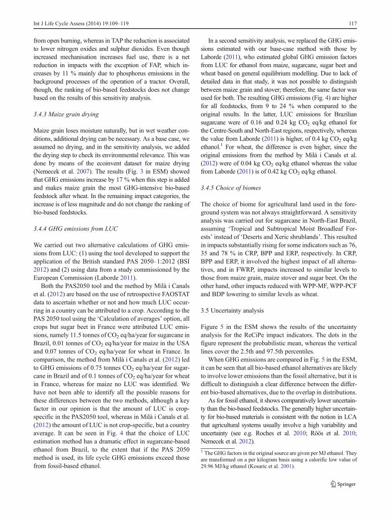
3.1 GHG emissions

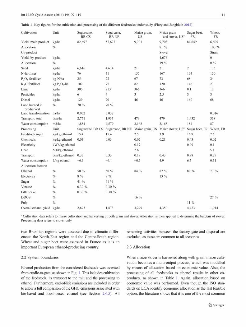
Figure 2 shows the GHG emissions of ethanol production fromcradle-to-gate plus the emissions from its degradation in theenvironment at the end-of-life. CO2 eq emissions from cradle-to-gate range from 0.7 to 1.5 kg per kg ethanol and from 1.3 to2 kg per kg ethanol if emissions from degradation at end-of-life

0.0

0.5

1.0

1.5

2.0

2.5

3.0

3.5

4.0

Sugarcane, BR CS

Sugarcane, BR NE

Maize grain, US

Maize stover, US

Sugar beet, FR

Wheat, FR Fossil, RER

kg C

O2-

eq/k

g et

hano

l

End-of-life Electricity Heat, from natural gas

Combustion, bagasse Production, others LUC

Pre-harvest burning Cultivation, others

Fig. 2 GHG emissions of ethanol from different agricultural feedstocksand from fossil resources, including emissions from degradation ofethanol at the end-of-life phase (ethanol emitted to air)

Int J Life Cycle Assess (2014) 19:109–119 113

are included. Even though carbon in bio-based ethanol is bio-genic, there is a significant contribution from expected methaneemissions due to degradation when part of the ethanol ispartitioned to the water compartment (Muñoz et al. 2013). Forfossil-based ethanol, emissions are of 1.3 kg CO2-eq fromcradle-to-gate and of 3.7 kg CO2-eq when end-of-life degrada-tion emissions are included. The latter are higher than for bio-based ethanol due to the fossil origin of the carbon. Thus from acradle-to-grave perspective, bio-based ethanol can involve asignificant (ca. 50 %) GHG reduction when compared with itsfossil-based counterpart.

When the bio-based ethanol alternatives are compared, sugarbeet and maize stover appear as the least GHG-intensive feed-stock, whereas wheat is the most intensive, with twice as highGHG emissions per kilogram product. All the other feedstockshave similar emissions from cradle-to-gate, of around 1 kg CO2

eq per kg. The low impact of sugar beet is closely linked to itshigh yield. Sugarcane in the studied regions of Brazil also hashigh yields, but these alternatives are penalised by the emissionsrelated to pre-harvest burning and LUC, showing higher overallemissions than sugar beet. It can be seen that there is littledifference between the Brazilian regions: the Centre-Southregion has higher yields, but this is achieved bymeans of higherinputs of agrochemicals and energy (see Table 1). The lowemissions for maize stover are related to the fact that the impactof maize cultivation is shared between the two co-products(grain and stover), and the lower economic value of stoverbenefits the latter in terms of its share of impact. However,the difference between these two feedstocks in GHG emissionsis not as big as one could expect, due to the fact that harvestingstover as opposed to leaving it in the field necessitates anadditional fertiliser input to correct for the loss in nutrients.

GHG emissions from cradle-to-gate are available in theliterature for some of the feedstocks, although several method-ological aspects make the comparison difficult, such as howmultifunctionality is dealt with (allocation/system expansion)and the inclusion of LUC emissions. Ethanol from sugarcane inBrazil has been assessed with GHG emissions per kilogram of0.74 (Renouf et al. 2008) and 2.15 kg CO2 eq (California EPA2009). The first value is lower than the one obtained in this

study because it excludes LUC emissions, whereas the secondone is higher because it includes a global assessment of indirectLUC emissions. In our study, only indirect LUC emissionstaking place in Brazil were taken into account. Previous studieson maize ethanol in the USA (California EPA 2009) highlightthe same aspect, namely the importance of whether or not andhow LUC emissions are dealt with. In the sensitivity analysis,further discussion on LUC and GHG emissions is provided.

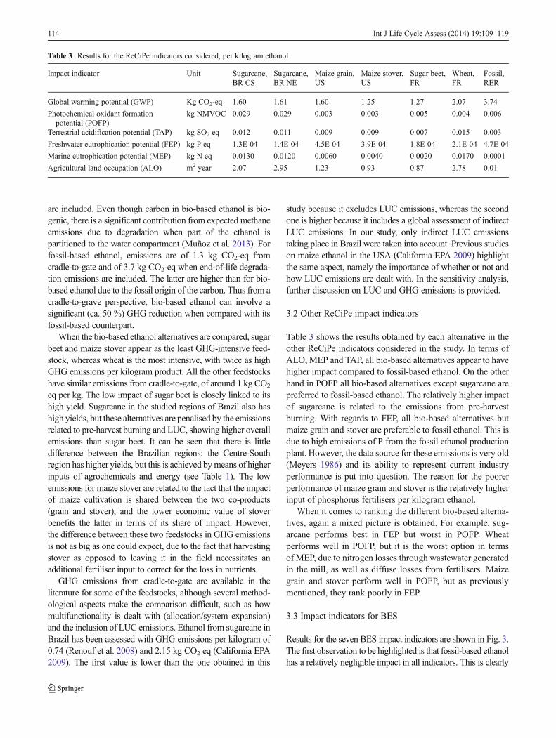
3.2 Other ReCiPe impact indicators

Table 3 shows the results obtained by each alternative in theother ReCiPe indicators considered in the study. In terms ofALO, MEP and TAP, all bio-based alternatives appear to havehigher impact compared to fossil-based ethanol. On the otherhand in POFP all bio-based alternatives except sugarcane arepreferred to fossil-based ethanol. The relatively higher impactof sugarcane is related to the emissions from pre-harvestburning. With regards to FEP, all bio-based alternatives butmaize grain and stover are preferable to fossil ethanol. This isdue to high emissions of P from the fossil ethanol productionplant. However, the data source for these emissions is very old(Meyers 1986) and its ability to represent current industryperformance is put into question. The reason for the poorerperformance of maize grain and stover is the relatively higherinput of phosphorus fertilisers per kilogram ethanol.

When it comes to ranking the different bio-based alterna-tives, again a mixed picture is obtained. For example, sug-arcane performs best in FEP but worst in POFP. Wheatperforms well in POFP, but it is the worst option in termsof MEP, due to nitrogen losses through wastewater generatedin the mill, as well as diffuse losses from fertilisers. Maizegrain and stover perform well in POFP, but as previouslymentioned, they rank poorly in FEP.

3.3 Impact indicators for BES

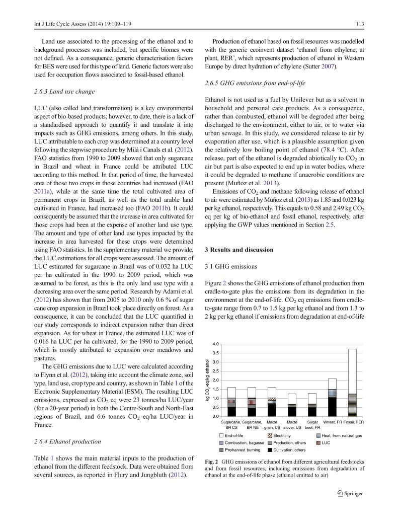
Results for the seven BES impact indicators are shown in Fig. 3.The first observation to be highlighted is that fossil-based ethanolhas a relatively negligible impact in all indicators. This is clearly

Table 3 Results for the ReCiPe indicators considered, per kilogram ethanol

Impact indicator Unit Sugarcane,BR CS

Sugarcane,BR NE

Maize grain,US

Maize stover,US

Sugar beet,FR

Wheat,FR

Fossil,RER

Global warming potential (GWP) Kg CO2-eq 1.60 1.61 1.60 1.25 1.27 2.07 3.74

Photochemical oxidant formationpotential (POFP)

kg NMVOC 0.029 0.029 0.003 0.003 0.005 0.004 0.006

Terrestrial acidification potential (TAP) kg SO2 eq 0.012 0.011 0.009 0.009 0.007 0.015 0.003

Freshwater eutrophication potential (FEP) kg P eq 1.3E-04 1.4E-04 4.5E-04 3.9E-04 1.8E-04 2.1E-04 4.7E-04

Marine eutrophication potential (MEP) kg N eq 0.0130 0.0120 0.0060 0.0040 0.0020 0.0170 0.0001

Agricultural land occupation (ALO) m2 year 2.07 2.95 1.23 0.93 0.87 2.78 0.01

114 Int J Life Cycle Assess (2014) 19:109–119

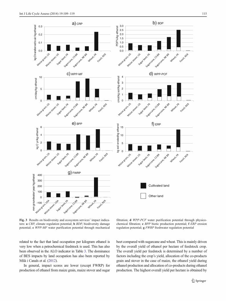
related to the fact that land occupation per kilogram ethanol isvery low when a petrochemical feedstock is used. This has alsobeen observed in the ALO indicator in Table 3. The dominanceof BES impacts by land occupation has also been reported byMilà i Canals et al. (2012).

In general, impact scores are lower (except FWRP) forproduction of ethanol frommaize grain, maize stover and sugar

beet compared with sugarcane and wheat. This is mainly drivenby the overall yield of ethanol per hectare of feedstock crop.The overall yield per feedstock is determined by a number offactors including the crop’s yield, allocation of the co-productsgrain and stover in the case of maize, the ethanol yield duringethanol production and allocation of co-products during ethanolproduction. The highest overall yield per hectare is obtained by

Cultivated land

Other land

0.0

0.1

0.2

0.3

lonahtegk/ria

otderrefsnart

Cgk

a) CRP

0.0

0.5

1.0

1.5

2.0

2.5

3.0

PD

F%

/kg

eth

anol

b) BDP

0

5

10

cm/d

ay/k

g e

than

ol

c) WPP-MF

0

1

2

3

4

cmol

/kg

soi

l/kg

eth

anol

d) WPP-PCF

0

2

4

6

kg C

yr/

kg e

than

ol

e) BPP

0

5

10

15

kg s

oil e

rode

d/kg

eth

anol f) ERP

-100

0

100

200

300

400lonahtegk/raey/reta

wdnuorgm

m

g) FWRP

Fig. 3 Results on biodiversity and ecosystem services’ impact indica-tors: a CRP, climate regulation potential; b BDP, biodiversity damagepotential; c WPP-MF water purification potential through mechanical

filtration; d WPP-PCF water purification potential through physico-chemical filtration; e BPP biotic production potential; f ERP erosionregulation potential; g FWRP freshwater regulation potential

Int J Life Cycle Assess (2014) 19:109–119 115

the production chain from sugar beet followed by maize grainand stover (Table 1). On the other hand, the production chainwith sugarcane from the North-East region of Brazil followedby wheat yield the lowest output per hectare.

In the case of CRP (Fig. 3a), Müller-Wenk and Brandão(2010) argue that the results of this impact category shouldbe added to other GHG emissions (Fig. 1). We have not doneso in Fig. 1 because CRP relates to the ‘foregone sequestra-tion’, i.e. the amount of C not fixed in biomass due to a pastLUC, and not to actual GHG emissions. If CRP wasconverted to CO2 eq and added to the cradle-to-grave GHGemissions, the results would still be favourable for all optionsof bio-based ethanol when compared to fossil-based ethanol,although the performance of wheat-based ethanol would besignificantly eroded, with GHG emissions only 20 % lowerthan those of the fossil-based ethanol.

3.4 Sensitivity analyses

Several aspects were subject to a sensitivity analysis to checktheir influence on the results of the ReCiPe impact indicators.Below, we describe these analyses and the results obtained.

3.4.1 Allocation in ethanol production

Due to increased demand of ethanol as a fuel and basicchemical, its price could rise, therefore affecting the economicallocation in the production process. We modelled the systemassuming as that, as a worst case, 100 % of the environmentalburdens are allocated to ethanol and 0 % to any co-product

(DDGS, electricity, etc.). The results (Fig. 1 in ESM) showeda sharp increase in all impacts for ethanol from sugarcane, butmuch lower for the other feedstocks. Due to the equallyvaluable by-product sugar, the allocation factor for ethanolfrom sugarcane is doubled, resulting in a doubled score in allimpacts, with the exception of GHG emissions, which in-crease by 63 %. However, given that there is an increasingglobal demand for sugar, it is unlikely that 100 % of therevenue from sugarcane products will be attributed to ethanolin the future. In terms of overall ranking of feedstocks, thissensitivity analysis does not change the main results obtained,i.e. bio-based feedstocks still present lower GHG emissionsthan fossil-based ethanol, but the former are still more impact-ful in many of the other ReCiPe impact categories.

3.4.2 Pre-harvest burning of sugar cane

The Brazilian State of Sao Paulo aims for zero pre-harvestburning in 2021. This will lead to a reduction in impacts fromopen burning of biomass but also to increased mechanisation.When sugarcane is modelled without pre-harvest burning,there is a reduction in impacts (Fig. 2 in ESM), most notablyin POFP (66 % reduction), but also in other indicators such asGHG emissions (9 % reduction) and TAP (20 % reduction).The big reduction in the POFP category is related to theavoidance of emissions of volatile organic hydrocarbons, ni-trogen oxides and sulphur dioxide from open burning, whichare key contributors to this impact category. Similarly, in theclimate change impact category, the reduction is associatedwith avoiding the dinitrogen monoxide and methane emissions

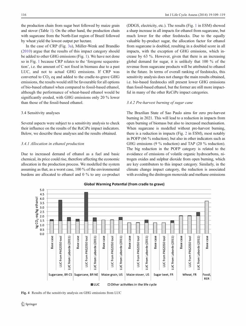
Fig. 4 Results of the sensitivity analysis on GHG emissions from LUC

116 Int J Life Cycle Assess (2014) 19:109–119

from open burning, whereas in TAP the reduction is associatedto lower nitrogen oxides and sulphur dioxides. Even thoughincreased mechanisation increases fuel use, there is a netreduction in impacts with the exception of FAP, which in-creases by 11 % mainly due to phosphorus emissions in thebackground processes of the operation of a tractor. Overall,though, the ranking of bio-based feedstocks does not changebased on the results of this sensitivity analysis.

3.4.3 Maize grain drying

Maize grain loses moisture naturally, but in wet weather con-ditions, additional drying can be necessary. As a base case, weassumed no drying, and in the sensitivity analysis, we addedthe drying step to check its environmental relevance. This wasdone by means of the ecoinvent dataset for maize drying(Nemecek et al. 2007). The results (Fig. 3 in ESM) showedthat GHG emissions increase by 17 % when this step is addedand makes maize grain the most GHG-intensive bio-basedfeedstock after wheat. In the remaining impact categories, theincrease is of less magnitude and do not change the ranking ofbio-based feedstocks.

3.4.4 GHG emissions from LUC

We carried out two alternative calculations of GHG emis-sions from LUC: (1) using the tool developed to support theapplication of the British standard PAS 2050–1:2012 (BSI2012) and (2) using data from a study commissioned by theEuropean Commission (Laborde 2011).

Both the PAS2050 tool and the method by Milà i Canalset al. (2012) are based on the use of retrospective FAOSTATdata to ascertain whether or not and how much LUC occur-ring in a country can be attributed to a crop. According to thePAS 2050 tool using the ‘Calculation of averages’ option, allcrops but sugar beet in France were attributed LUC emis-sions, namely 11.5 tonnes of CO2 eq/ha/year for sugarcane inBrazil, 0.01 tonnes of CO2 eq/ha/year for maize in the USAand 0.07 tonnes of CO2 eq/ha/year for wheat in France. Incomparison, the method from Milà i Canals et al. (2012) ledto GHG emissions of 0.75 tonnes CO2 eq/ha/year for sugar-cane in Brazil and of 0.1 tonnes of CO2 eq/ha/year for wheatin France, whereas for maize no LUC was identified. Wehave not been able to identify all the possible reasons forthese differences between the two methods, although a keyfactor in our opinion is that the amount of LUC is crop-specific in the PAS2050 tool, whereas in Milà i Canals et al.(2012) the amount of LUC is not crop-specific, but a countryaverage. It can be seen in Fig. 4 that the choice of LUCestimation method has a dramatic effect in sugarcane-basedethanol from Brazil, to the extent that if the PAS 2050method is used, its life cycle GHG emissions exceed thosefrom fossil-based ethanol.

In a second sensitivity analysis, we replaced the GHG emis-sions estimated with our base-case method with those byLaborde (2011), who estimated global GHG emission factorsfrom LUC for ethanol from maize, sugarcane, sugar beet andwheat based on general equilibrium modelling. Due to lack ofdetailed data in that study, it was not possible to distinguishbetween maize grain and stover; therefore, the same factor wasused for both. The resulting GHG emissions (Fig. 4) are higherfor all feedstocks, from 9 to 24 % when compared to theoriginal results. In the latter, LUC emissions for Braziliansugarcane were of 0.16 and 0.24 kg CO2 eq/kg ethanol forthe Centre-South and North-East regions, respectively, whereasthe value from Laborde (2011) is higher, of 0.4 kg CO2 eq/kgethanol.1 For wheat, the difference is even higher, since theoriginal emissions from the method by Milà i Canals et al.(2012) were of 0.04 kg CO2 eq/kg ethanol whereas the valuefrom Laborde (2011) is of 0.42 kg CO2 eq/kg ethanol.

3.4.5 Choice of biomes

The choice of biome for agricultural land used in the fore-ground system was not always straightforward. A sensitivityanalysis was carried out for sugarcane in North-East Brazil,assuming ‘Tropical and Subtropical Moist Broadleaf For-ests’ instead of ‘Deserts and Xeric shrublands’. This resultedin impacts substantially rising for some indicators such as 76,35 and 78 % in CRP, BPP and ERP, respectively. In CRP,BPP and ERP, it involved the highest impact of all alterna-tives, and in FWRP, impacts increased to similar levels tothose from maize grain, maize stover and sugar beet. On theother hand, other impacts reduced with WPP-MF, WPP-PCFand BDP lowering to similar levels as wheat.

3.5 Uncertainty analysis

Figure 5 in the ESM shows the results of the uncertaintyanalysis for the ReCiPe impact indicators. The dots in thefigure represent the probabilistic mean, whereas the verticallines cover the 2.5th and 97.5th percentiles.

When GHG emissions are compared in Fig. 5 in the ESM,it can be seen that all bio-based ethanol alternatives are likelyto involve lower emissions than the fossil alternative, but it isdifficult to distinguish a clear difference between the differ-ent bio-based alternatives, due to the overlap in distributions.

As for fossil ethanol, it shows comparatively lower uncertain-ty than the bio-based feedstocks. The generally higher uncertain-ty for bio-based materials is consistent with the notion in LCAthat agricultural systems usually involve a high variability anduncertainty (see e.g. Roches et al. 2010; Röös et al. 2010;Nemecek et al. 2012).

1 The GHG factors in the original source are given per MJ ethanol. Theyare transformed on a per kilogram basis using a calorific low value of29.96 MJ/kg ethanol (Kosaric et al. 2001).

Int J Life Cycle Assess (2014) 19:109–119 117

Overall, like in the deterministic modelling, the fossil ethanolshows clear advantages in MEP, TAP and ALO, whereas thebest-performing bio-based alternatives in these indicators aresugarcane and sugar beet (MEP) and sugar beet (TAP, ALO).

4 Conclusions

LCAwas applied to assess the global bio-based commodityethanol, from several biomass sources and regions in theworld. Bio-based ethanol was also compared to its fossil-based counterpart, produced from ethylene.

The results have shown that GHG emissions from cradle-to-gate for the bio-based ethanol production routes assessedvary by a factor of up to 5, with the sugar beet route in Franceshowing the lowest emissions and wheat showing thehighest, unless GHG emissions from LUC are assessed withthe PAS 2050 tool for horticultural products, in which casesugarcane-based ethanol from Brazil shows the highest GHGemissions. Looking at cradle-to-grave emissions, all bio-based ethanol production routes involve lower emissionsthan fossil-based ethanol, with the exception of sugarcane-based ethanol, provided that GHG emissions from LUC areassessed with the PAS 2050 tool for horticultural products.

When other impact indicators are considered, trade-offs ap-pear between bio-based and fossil-based ethanol. The latterperforms better in all BES impact indicators as well as in agri-cultural land occupation, marine eutrophication and terrestrialacidification. A parallel water footprint study also clearly showeda much lower water demand and impacts on water scarcity fromfossil-based ethanol (Flury et al. 2012). In terms of the novelBES impact categories considered in this study, they allowed toclearly identifying fossil-based ethanol as the preferred alterna-tive, and this is linked to its lower land occupation. On the otherhand, when comparing bio-based ethanol production routes, thechoice of biomes was not straightforward. This is an area thatrequires further guidance for practitioners.

This latter conclusion also points to the general issue oftrading climate change for land use impacts when transitioningto a bio-based economy. This transition may be unavoidable inthe face of climate change and fossil resource depletion, butadequate consideration of impacts on BES will be required inorder to minimise detrimental trade-offs.

The biomass feedstock showing the best environmentalperformance in most indicators assessed was sugar beet, andthis is clearly linked to the high yields of this crop. Withregard to ethanol from sugarcane grown in the two assessedregions of Brazil, differences were found to be small in allimpact indicators. However, water consumption was foundto be three times higher in the North-East region whencompared to the Centre-South region by Flury et al. (2012).

In general, we can conclude that environmental impacts frombio-based ethanol are highly dependent on the characteristics of

the production chain considered, as well as on modelling andscenario choices, such as the choice of allocation factors, or theneed to dry the product after harvest. However, key factors foundin this study to describe the environmental impacts of bio-basedproducts are the net product yield per hectare and year (combi-nation of agricultural yield plus yield in the processing stage) andespecially modelling of emissions caused by LUC. Given theincreasing importance of bio-based products in the global econ-omy, we call the LCA community to initiate a debate to harmo-nise the modelling of LUC emissions.

References

Adami M, Rudorff BFT, Freitas RM, Aguiar DA, Sugawara LM, Mello MP(2012) Remote sensing time series to evaluate land use change of recentexpanded sugar cane crop in Brazil. Sustainability, 4(4):574–585

ADEME (2010) Analyses de Cycle de Vie appliquées aux biocarburantsde première génération consommés en France. Direction Productionet Energies Durables (DEPD), France

Ardente F, Cellura M (2011) Economic allocation in life cycle assess-ment. The state of the art and discussion of examples. J Ind Ecol16(3):387–398

Biofuels Platform (2010) Production of biofuels in the world in 2009.Geographic distribution of bioethanol and biodiesel production in theworld. http://www.biofuels-platform.ch/en/infos/production.php?id=bioethanol. Accessed 08 June 2012

BSI (2012) PAS 2050–1: 2012 assessment of life cycle greenhouse gasemissions from horticultural products. Supplementary require-ments for the cradle to gate stages of GHG assessments of horti-cultural products undertaken in accordance with PAS 2050. BritishStandards Institution, London

Brandão M, Milà i Canals L (2012) Global characterisation factors toassess land use impacts on biotic production. Int J Life CycleAssess. doi:10.1007/s11367-012-0381-3

California EPA (2009) Proposed regulation to implement the low car-bon fuel standard, volume I. Staff Report: Initial Statement ofReasons. California Environmental Protection Agency, CaliforniaAir Resources Board, Sacramento

de Baan L, Alkemade R, Koellner T (2012) Land use impacts onbiodiversity in LCA: a global approach. Int J Life Cycle Assess.doi:10.1007/s11367-012-0412-0

de Jong E, Higson A,Walsh P, Wellisch M (2012) Bio-based chemicals,value added products from biorefineries. IEA Bioenergy, Task42Biorefinery

De Klein C, Novoa RSA, Ogle S, Smith KA, Rochette P, Wirth TC,McConkey BG, Mosier A, Rypdal K, Walsh M, Williams SA(2006) N2O emissions from managed soils, and CO2 emissionsfrom lime and urea application. In: Eggleston HS, Buendia L,Miwa K, Ngara T, Tanabe K. (eds.) IPCC Guidelines for NationalGreenhouse Gas Inventories. IGES, Japan. Vol 4, chapter 11

FAO (2010) Bioenergy environmental impact analysis (BIAS). Foodand Agriculture Organization of the United Nations, Rome

FAO (2011a) FAOSTAT. http://faostat.fao.org/site/567/default.aspx#ancor. Accessed 13 June 2012

FAO (2011b) FAOSTAT. http://faostat.fao.org/site/377/default.aspx#ancor. Accessed 13 June 2012

Flury K, Jungbluth N (2012) Greenhouse gas emissions and waterfootprint of ethanol from maize, sugar cane, wheat and sugar beet.ESU-services, Uster, Switzerland

Flury K, Frischknecht R, Jungbluth N,Muñoz I (2012) Recommendation forlife cycle inventory analysis for water use and consumption. Working

118 Int J Life Cycle Assess (2014) 19:109–119

paper, ESU Services. http://www.esu-services.ch/fileadmin/download/flury-2012-water-LCI-recommendations.pdf. Accessed 8 Aug 2013

Flynn HC, Milà iCanals L, Keller E, King H, Sim S, Hastings A, WangS, Smith P (2012) Quantifying global greenhouse gas emissionsfrom land-use change for crop production. Glob Change Biol18(5):1622–1635

Frischknecht R, Jungbluth N, Althaus H-J, Doka G, Dones R, HischierR, Hellweg S, Nemecek T, Rebitzer G, Spielmann M (2010)Overview and methodology. Final report ecoinvent data v2.2,No. 1. Swiss Centre for Life Cycle Inventories, Dübendorf

Fu ZG, Chan AW,Minns DE (2003) Lyfe cycle assessment of bio-ethanolderived from cellulose. Int J Life Cycle Assess 8(3):137–141

Goedkoop M, Heijungs R, Huijbregts M, De Schryver A, Struijs J, vanZelm R (2009) ReCiPe 2008 A life cycle impact assessmentmethod which comprises harmonised category indicators at themidpoint and the endpoint level. First edition. Report I: character-isation. Ministry of housing, Spatial Planning and Environment(VROM), The Netherlands

Jungbluth N, Chudacoff M, Dauriat A, Dinkel F, Doka G, FaistEmmenegger M, Gnansounou E, Kljun N, Schleiss K, SpielmannM, Stettler C, Sutter J (2007) Life cycle inventories of bioenergy.ecoinvent report no. 17, v2.0. ESU-services, Uster

Kim S, Dale BE (2009) Regional variations in greenhouse gas emis-sions of biobased products in the United States—corn-based eth-anol and soybean oil. Int J Life Cycle Assess 14:540–546

Koellner T, de Baan L, Brandão M, Milà i Canals L, Civit B, Margni M,Saad R, Maia de Souza D, Beck T, Müller-Wenk R (2013) UNEP-SETAC guideline on global land use impact assessment on biodi-versity and ecosystem services in LCA. Int J Life Cycle Assess.doi:10.1007/s11367-013-0579-z

Kosaric N, Duvnjak Z, Farkas A, Sahm H, Binger-Meyer S, Goebel O,Mayer D et al (2001) Ethanol. In: Arpe (ed) Ullmann’s encyclopediaof industrial chemistry: electronic release, 6th edn.Wiley,Weinheim

Laborde D (2011) Assessing the land use change consequences ofEuropean biofuel policies, final report. Prepared by the Interna-tional Food Policy Institute (IFPRI) for the European Commission.Specific Contract No SI2. 580403, implementing FrameworkContract No TRADE/07/A2

Linak E, Janshekar H, Inoguchi Y (2009) Ethanol. Chemical economicshandbook research report. SRI Consulting, Houston

Macedo IC, Seabra JEA, Silva JEAR (2008) Green house gases emis-sions in the production and use of ethanol from sugarcane inBrazil: The 2005/2006 averages and a prediction for 2020. Bio-mass Bioenerg 32:582–595

Meyers R (1986) Handbook of chemical production processes.McGraw-Hill, New York

MilàiCanals L, Rigarlsford G, Sim S (2012) Land use impact assessment ofmargarine. Int J Life Cycle Assess. doi:10.1007/s11367-012-0380-4

Miller SA, Landis AE, Theis TL (2007) Environmental trade-offs ofbiobased production. Environ Sci Technol 41(15):5176–5182

Müller-Wenk R, Brandão M (2010) Climatic impact of land use inLCA—carbon transfers between vegetation/soil and air. Int J LifeCycle Assess 15:172–182

Muñoz I, Rigarlsford G, Milà i Canals L, King H (2013) Accounting forgreenhouse-gas emissions from the degradation of chemicals inthe environment. Int J Life Cycle Assess 18(1):252–262

Nemecek T, Heil A, Huguenin O, Meier S, Erzinger S, Blaser S, Dux D,Zimmermann A (2007) Life cycle inventories of agricultural pro-duction systems. Ecoinvent report no. 15, v2.0. Agroscope FALReckenholz and FAT Taenikon, Swiss Centre for Life Cycle In-ventories, Dübendorf

Nemecek T, Weiler K, Plassmann K, Schnetzer J, Gaillard G, JefferiesD, García–Suárez T, King H, Milà i Canals L (2012) Estimation ofthe variability in global warming potential of global crop produc-tion using a modular extrapolation approach (MEXALCA). JClean Prod 31:106–117

Nguyen TT, Gheewala SH (2008a) Life cycle assessment of fuel ethanolfrom cassava in Thailand. Int J Life Cycle Assess 13(2):147–154

Nguyen TT, Gheewala SH (2008b) Life cycle assessment of fuel etha-nol from cane molasses in Thailand. Int J Life Cycle Assess13(4):301–311

Ometto AR, Hauschild MZ, Lopes Roma WN (2009) Lifecycle assess-ment of fuel ethanol from sugarcane in Brazil. Int J Life CycleAssess 14:236–247

Pré Consultants (2012) Simapro software. http://www.pre-sustainability.com/content/simapro-lca-software. Accessed 08 June 2012

Renouf MA, Wegener MK, Nielsen LK (2008) An environmental lifecycle assessment comparing Australian sugarcane with US cornand UK sugar beet as producers of sugars for fermentation. Bio-mass Bioenerg 32:1144–1155

Roches A, Nemecek T, Gaillard G, Plassmann K, Sim S, King H, Milà iCanals L (2010) MEXALCA: a modular method for the extrapo-lation of crop LCA. Int J Life Cycle Assess 15(8):842–854

Röös E, Sundberg C, Hansson P-A (2010) Uncertainties in the carbonfootprint of food products: a case study on table potatoes. Int J LifeCycle Assess 15:478–488

Saad R, Koellner T, Margni M (2013) Land use impacts on freshwaterregulation, erosion regulation and water purification: a spatialapproach for a global scale level. Int J Life Cycle Assess.doi:10.1007/s11367-013-0577-1

Silalertruksa T, Gheewala SH (2011) Long-term bioethanol system andits implications on GHG emissions: a case study of Thailand.Environ Sci Technol 45:4920–4928

Stewart LK, Charlesworth PB, Bristow KL (2003) Estimating nitrateleaching under a sugarcane crop using APSIM-SWIM. Proceed-ings from: MODSIM 2003 International Congress on Modellingand Simulation, Modelling and Simulation Society of Australiaand New Zealand, July 2003

Sutter J (2007) Life cycle inventories of petrochemical solvents.ecoinvent report No. 22, v2.0. ETH Zürich. Swiss Centre for LifeCycle Inventories, Dübendorf

Tsao CC, Campbell JE, Mena-Carrasco M, Spak SN, Carmichael GR,Chen Y (2011) Increased estimates of air-pollution emissions fromBrazilian sugar-cane ethanol. Nat Clim Chang 2:53–57

USEPA (2010) Renewable fuel standard program (RFS2) regulatoryimpact analysis. EPA-420-R-10-006

Int J Life Cycle Assess (2014) 19:109–119 119