level of service
DESCRIPTION
los-characteristicTRANSCRIPT

1
Chapter 6
Highway Capacity and Level of Service Analysis
Seek to measure Highway Performance (Congestion). Needed for:
Highway construction
Congestion relief

2
Problems:
Wide variation of highway conditions:
Different roadway types (Freeway, multilane, etc.)
Number of lanes and width of lanes
Vehicle mix (cars vs. trucks)
Shoulder widths
Temporal variation in traffic flow over the day and over the peak hour

6.1 LEVEL OF SERVICE CONCEPT
The level of service provides a qualitative ranking of the traffic operational conditions experienced by users of a facility
Highway Capacity Manual defines the LOS categories for freeways and multilane highways as follows:

4
Level of Service A free-flow conditions (traffic operates at free flow speeds as defined in Chapter 5). Individual users are virtually unaffected by the presence of others in the traffic stream. Freedom to select desired speeds and to maneuver within the traffic stream is extremely high. The general level of comfort and convenience provided to drivers is excellent.

Level of Service B allows speeds at or near free-flow speeds, but the presence of other users in the traffic stream begins to be noticeable. Freedom to select desired speeds is relatively unaffected, but there is a slight decline in the freedom to maneuver within the traffic stream relative to LOS A.

6
Level of Service C speeds at or near free-flow speeds, but the freedom to maneuver is noticeably restricted (lane changes require careful attention on the part of drivers). The general level of comfort and convenience declines significantly at this level. Disruptions in the traffic stream, such as an incident (for example, vehicular accident or disablement), can result in significant queue formation and vehicular delay. In contrast, the effect of incidents at LOS A or LOS B are minimal, and cause only minor delay in the immediate vicinity of the event.

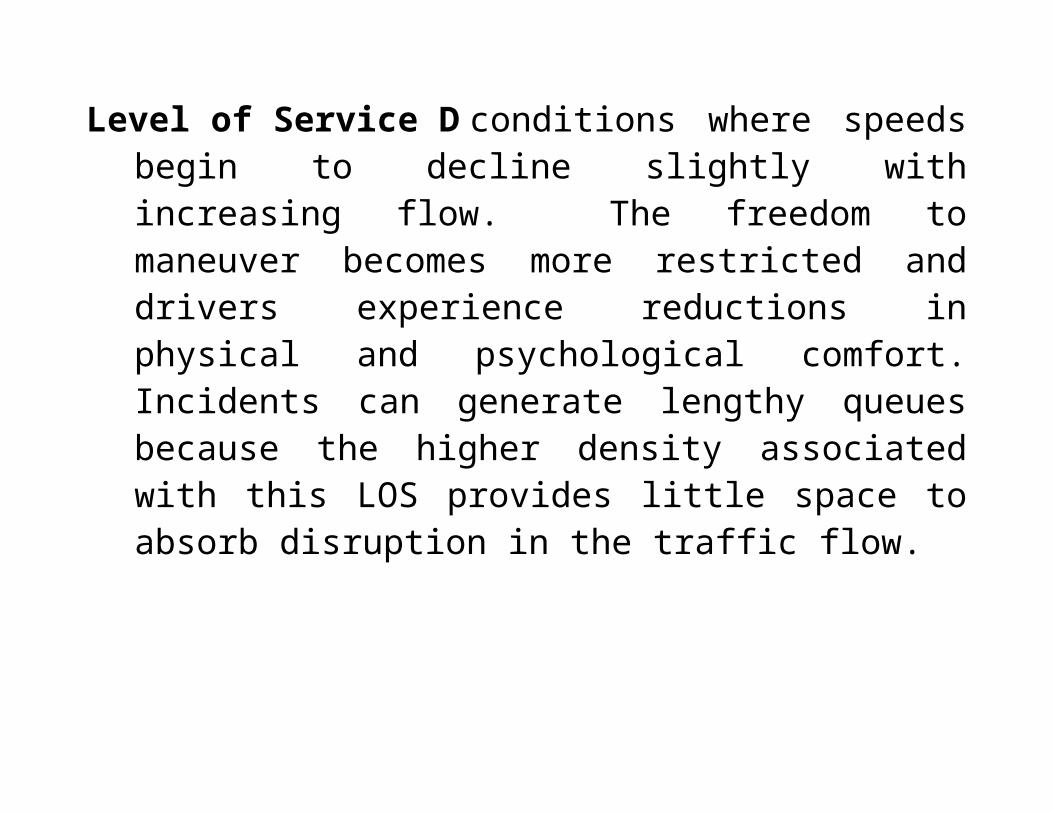
Level of Service D conditions where speeds begin to decline slightly with increasing flow. The freedom to maneuver becomes more restricted and drivers experience reductions in physical and psychological comfort. Incidents can generate lengthy queues because the higher density associated with this LOS provides little space to absorb disruption in the traffic flow.

8
Level of Service E LOS E represents operating conditions at or near the roadway’s capacity. Even minor disruptions to the traffic stream, such as vehicles entering from a ramp or vehicles changing lanes, can cause delays as other vehicles give way to allow such maneuvers. In general, maneuverability is extremely limited and drivers experience considerable physical and psychological discomfort.

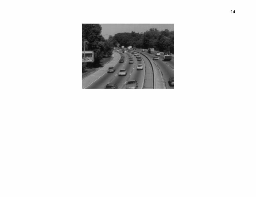
Level of Service F describes a breakdown in vehicular flow. Queues form quickly behind points in the roadway where the arrival flow rate temporarily exceeds the departure rate, as determined by the roadway’s capacity (Chapter 5). Vehicles typically operate at low speeds in these conditions and are often required to come to a complete stop, usually in a cyclic fashion. The cyclic formation and dissipation of queues is a key characterization of LOS F.

10
LOS A

12
LOS B

14
LOS C

LOS D

16

LOS E
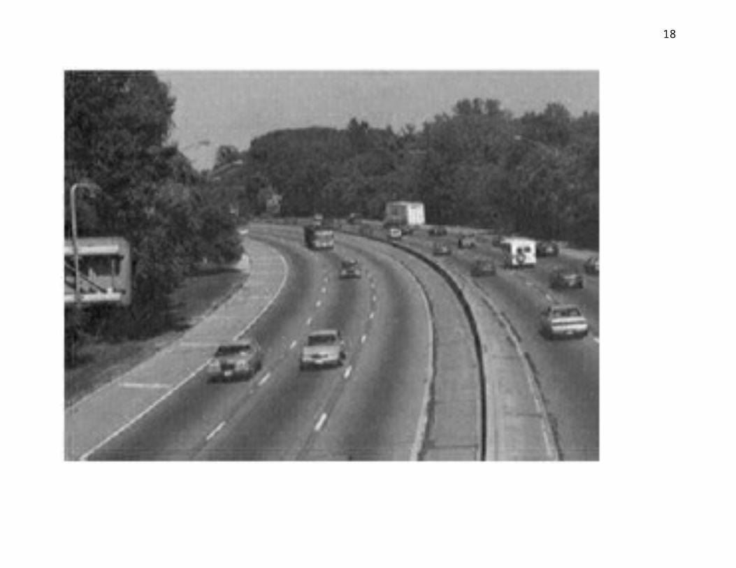
18
LOS F

6.2 LEVEL OF SERVICE DETERMINATION
6.2.1 Base Conditions
lane widths,
lateral clearances,
access frequency (non access controlled highways),
terrain;
traffic stream conditions such as the effects of heavy vehicles (large trucks, buses and RVs), and
driver population characteristics.

20
Process:
1. Free-Flow Speed
The free-flow speed (FFS) is the mean speed of traffic as measured when flow rates are low to moderate (specific values are given under the individual sections for each roadway type).

2. Analysis Flow Rate
The highest volume in a 24-hour period (the peak-hour volume) is used for V in traffic analysis computations. However, this hourly volume is adjusted for:
The temporal variation of traffic demand within the analysis hour,
the impacts due to heavy vehicles and,
characteristics of the driving population.
3. Determine LOS

22
6.3 BASIC FREEWAY SEGMENTS
6.3.1 Base Conditions and Capacity 3.6 m (12-ft) (minimum lane widths, 1.8 m (6-ft) minimum right-shoulder clearance between
edge of travel lane and objects (utility poles, retaining walls, etc.) that influence driver behavior,
0.6 m (2-ft) minimum median lateral clearance, only passenger cars in the traffic stream, 5 or more lanes in each travel direction (urban areas only), 3 km (2-mi) or greater interchange spacing, level terrain (no grades greater than 2%), and a driver population of mostly familiar roadway users.

Capacity:Table 6.2 The Relationship Between Free-Flow Speed and
Capacity on Basic Freeway Segments
Free-Flow Speed(mi/h)
Capacity(pc/h/ln)
Free-Flow Speed(km/h)
Capacity(pc/h/ln)
75 2400 120 240070 2400 110 235065 2350 100 230060 2300 90 225055 2250

24
6.3.2 Service Measure The service measure for basic freeway segments is density.
Density, as discussed in Chapter 5, is typically measured in terms of passenger cars per mile per lane (pc/mi/ln) (pc/km/ln), and therefore provides a good measure of the relative mobility of individual vehicles in the traffic stream.
Recalling Eq. 5.14 from Chapter 5,
q = uk (6.1)
Where:q = flow in veh/h, u = speed in mi/h (km/h) and, k = density in veh/mi (veh/km).

So density is therefore calculated as flow divided by speed.
Once the flow and speed values have been determined according to the given conditions, a density can be calculated and then referenced in Table 6.1 or Fig. 6.2 to arrive at a level of service for the freeway segment.

Table 6.1 LOS Criteria for Basic Freeway SegmentsCriteria
LOSA B C D E
FFS = 75 mi/hMaximum density (pc/mi/ln) 11 18 26 35 45Average speed (mi/h) 75.0 74.8 70.6 62.2 53.3Maximum v/c 0.34 0.56 0.76 0.90 1.00Maximum service flow rate (pc/h/ln)
820 1350 1830 2170 2400
FFS = 70 mi/hMaximum density (pc/mi/ln) 11 18 26 35 45Average speed (mi/h) 70.0 70.0 68.2 61.5 53.3Maximum v/c 0.32 0.53 0.74 0.90 1.00Maximum service flow rate (pc/h/ln)
770 1260 1770 2150 2400
FFS = 65 mi/hMaximum density (pc/mi/ln) 11 18 26 35 45Average speed (mi/h) 65.0 65.0 64.6 59.7 52.2Maximum v/c 0.30 0.50 0.71 0.89 1.00Maximum service flow rate (pc/h/ln)
710 1170 1680 2090 2350
FFS = 60 mi/hMaximum density (pc/mi/ln) 11 18 26 35 45Average speed (mi/h) 60.0 60.0 60.0 57.6 51.1Maximum v/c 0.29 0.47 0.68 0.88 1.00Maximum service flow rate (pc/h/ln)
660 1080 1560 2020 2300
FFS = 55 mi/hMaximum density (pc/mi/ln) 11 18 26 35 45Average speed (mi/h) 55.0 55.0 55.0 54.7 50.0Maximum v/c 0.27 0.44 0.64 0.85 1.00Maximum service flow rate (pc/h/ln)
600 990 1430 1910 2250

NOTE: The exact mathematical relationship between density and v/c has not always been maintained at LOS boundaries because of the use of rounded values. Density is the primary determinant of LOS. The speed criterion is the speed at maximum density for a given LOS. LOS F is characterized by highly unstable and variable traffic flow. Prediction of accurate flow rate, density, and speed at LOS F is difficult.

Figure 6.1 Basic Freeway Segment Speed-Flow Curves and Level of Service Criteria.
How reasonable is using just density to measure LOS?
Car drivers believe worse level of service if:
Higher density Only 4-lane freeway Between 21 and 65 years old College graduate Do not use freeway every day Do not regularly drive to work Lower average speed Higher standard deviation for speed Higher flow
Higher percentage of trucks Bad visibility (fog etc.) Higher standard deviation of headways
Truckers believe worse level of service if:
Drive less than 40,000 miles/year Higher density Only 4-lane freeway Higher standard deviation for speed Higher standard deviation of headways Lower percentage of trucks

6.3.3 Determining Free-Flow Speed
The FFS for basic freeway segments is the mean speed of passenger cars operating in flow rates up to 1300 passenger cars per hour per lane (pc/h/ln).
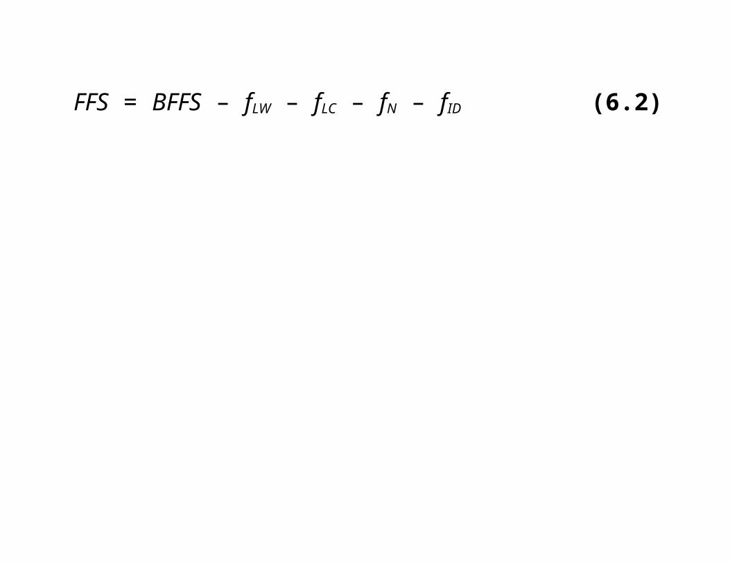
If the FFS is to be estimated rather than measured, the following equation can be used, which accounts for the roadway characteristics of lane width, right-shoulder lateral clearance, number of lanes, and interchange density.
FFS = BFFS – fLW – fLC – fN – fID (6.2)

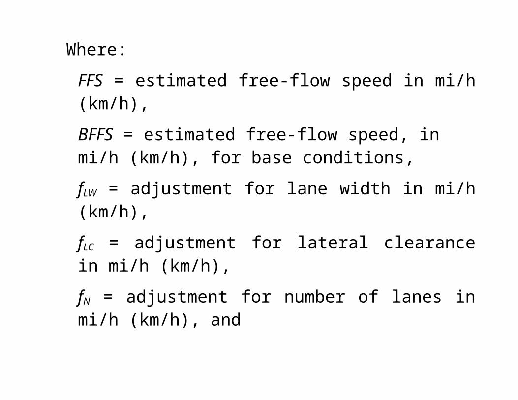
Where:
FFS = estimated free-flow speed in mi/h (km/h),
BFFS = estimated free-flow speed, in mi/h (km/h), for base conditions,
fLW = adjustment for lane width in mi/h (km/h),
fLC = adjustment for lateral clearance in mi/h (km/h),
fN = adjustment for number of lanes in mi/h (km/h), and
fID = adjustment for interchange density in mi/h (km/h).
The BFFS is assumed to be : 110 km/h (70 mi/h) for freeways in urban areas, and 120 km/h (75 mi/h) for freeways in rural areas.

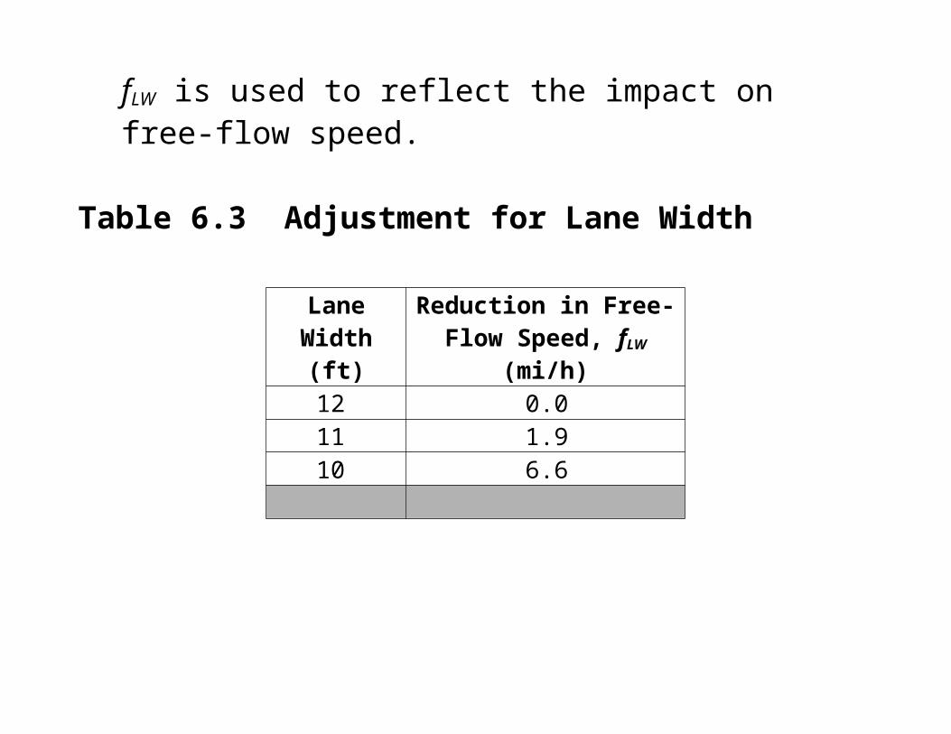
Lane Width Adjustment
When lane widths are narrower than the base 3.6m (12 ft), the adjustment factor fLW is used to reflect the impact on free-flow speed.
Table 6.3 Adjustment for Lane Width
Lane Width (ft)
Reduction in Free-Flow Speed, fLW (mi/h)
12 0.011 1.910 6.6

Lateral Clearance Adjustment
When obstructions are closer than 1.8 m (6 ft) (at the roadside) from the traveled pavement the adjustment factor fLC is used to reflect the impact on FFS.
Table 6.4 Adjustment for Right-Shoulder Lateral Clearance
Right-Shoulder Lateral
Clearance (ft)
Reduction in Free-Flow Speed, fLC (mi/h)Lanes in One Direction
2 3 4 5
6 0.0 0.0 0.0 0.05 0.6 0.4 0.2 0.14 1.2 0.8 0.4 0.23 1.8 1.2 0.6 0.32 2.4 1.6 0.8 0.41 3.0 2.0 1.0 0.50 3.6 2.4 1.2 0.6

Number of Lanes Adjustment
A freeway segment with five or more lanes in a direction is the base condition with respect to free-flow speed. Adjustments in FFS for fewer directional lanes are shown in Table 6.5.
Table 6.5 Adjustment for Number of Lanes on Urban Freeways
Number of Lanes
(One Direction)
Reduction in Free-Flow Speed, fN
mi/h km/h 5 0.0 0.0
4 1.5 2.43 3.0 4.82 4.5 7.3
Note: For all rural freeway segments, fN is 0.0.

Interchange Density Adjustment
When interchanges are spaced more frequently than one every two miles (one every 3.2 km), the traffic disturbances generated from merging and diverging movements will reduce the FFS.
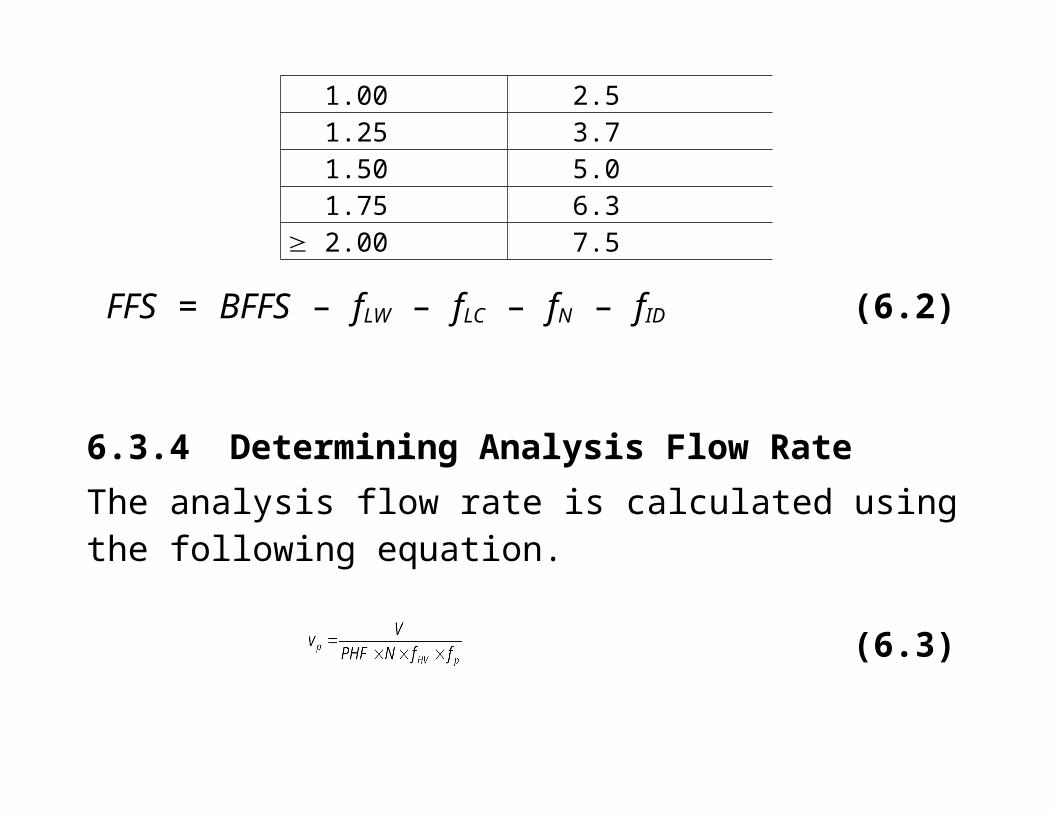
Table 6.6 Adjustment for Interchange Density
Interchanges per Mile
Reduction in Free-Flow Speed, fID (mi/h)
0.50 0.00.75 1.31.00 2.51.25 3.71.50 5.01.75 6.3
2.00 7.5

FFS = BFFS – fLW – fLC – fN – fID (6.2)
6.3.4 Determining Analysis Flow RateThe analysis flow rate is calculated using the following equation.
(6.3)
Where:
vp = 15-min passenger-car equivalent flow rate (pc/h/ln),V = hourly volume (veh/h),PHF = peak-hour factor,N = number of lanes,fHV = heavy-vehicle adjustment factor, and

fp = driver population factor.
6.3.4.1 Peak-Hour FactorTo account for this varying arrival rate, the peak 15-minute vehicle arrival rate within the analysis hour is used for practical traffic analysis purposes.
(6.4)Where:
PHF = peak-hour factor,V = hourly volume for hour of analysis,V15 = maximum 15-min flow rate within peak hour,
4 = number of 15-min periods per hour.

SF= service flow is the actual rate of flow for the peak 15-min period expanded to an hourly volume and expressed in vehicles per hour.
Equation 6.4 indicates that the further the PHF is from unity, the more peaked or nonuniform the traffic flow during the hour.
Example, consider two roads both of which have a peak-hour volume, V, of 1800 veh/h. The first road has 600 vehicles arriving in the highest 15-min interval and the second road has 500 vehicles arriving in the highest 15-min interval.
The first road has a more nonuniform flow, as indicated by a PHF of 0.75 [1800/(600 ´ 4)] that is further from unity than the second road’s PHF of 0.90 [1800/(500 ´ 4)].

6.3.4.2 Heavy Vehicle Adjustment
Large trucks, buses and recreational vehicles have performance characteristics (slow acceleration and inferior braking) and dimensions (length, height, and width) that have an adverse effect on roadway capacity.
The adjustment factor fHV is used to translate the traffic stream from base to prevailing conditions.

The fHV correction term is determined by first getting the passenger-car equivalent (PCE) for each large truck, bus, and/or recreational vehicle in the traffic stream.
These values represent the number of passenger cars that would consume the same amount of roadway capacity as a single large truck, bus, or recreational vehicle.
These passenger-car equivalents are denoted ET for large trucks and buses, and ER for recreational vehicles, and are a function of roadway grades because steep grades will tend to magnify the poor performance of heavy vehicles as well as the sight distance problems caused by their larger dimensions (the visibility afforded to drivers in vehicles following heavy vehicles).

For segments of freeway that contain a mix of grades, an extended segment analysis can be used as long as no single grade is steep enough or long enough to significantly impact the overall operations of the segment.
As a guideline, an extended segment analysis can be used for freeway segments where no single grade that is less than 3% is more than 0.5 mi (0.8 km) long, or no single grade that is 3% or greater is longer than 0.25 mi (0.4 km).
If an extended segment analysis is used, the terrain must be generally classified according to the following definitions:

Level Terrain Any combination of horizontal and vertical alignment permitting heavy vehicles to maintain approximately the same speed as passenger cars. This generally includes short grades of no more than 2%.
Rolling Terrain Any combination of horizontal and vertical alignment that causes heavy vehicles to reduce their speed substantially below those of passenger cars but does not cause heavy vehicles to operate at their limiting speed for the given terrain for any significant length of time or at frequent intervals (not having Fnet(V) = 0 due to high grade resistance as illustrated in Fig. 2.6).
Mountainous Terrain Any combination of horizontal and vertical alignment that causes heavy vehicles to operate at their limiting speed for significant distances or at frequent intervals.

Table 6.7 Passenger Car Equivalents (PCEs) for Extended Freeway Segments
Factor Type of TerrainLevel Rolling Mountainous
ET (trucks and buses) 1.5 2.5 4.5ER (RVs) 1.2 2.0 4.0
Any grade that does not meet the conditions for an extended segment analysis must be analyzed as a separate segment because of its significant impact on traffic operations. In these cases, grade-specific PCE values must be used.
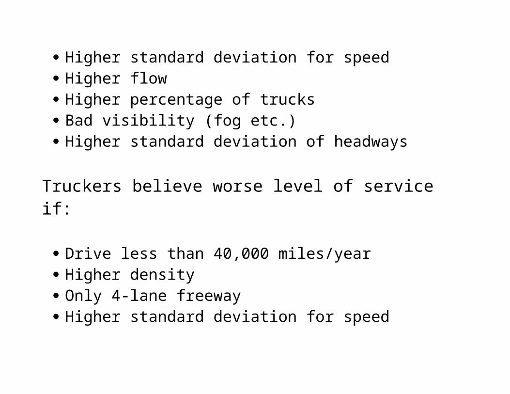
Table 6.8 Passenger Car Equivalents (PCEs) for Trucks and Buses on Specific Upgrades
Upgrade(%)
Length(mi)
ET
Percentage of Trucks and Buses2 4 5 6 8 10 15 20 25
< 2 All 1.5 1.5 1.5 1.5 1.5 1.5 1.5 1.5 1.5
2-3
0.0-0.25 1.5 1.5 1.5 1.5 1.5 1.5 1.5 1.5 1.5> 0.25-0.50 1.5 1.5 1.5 1.5 1.5 1.5 1.5 1.5 1.5> 0.50-0.75 1.5 1.5 1.5 1.5 1.5 1.5 1.5 1.5 1.5> 0.75-1.00 2.0 2.0 2.0 2.0 1.5 1.5 1.5 1.5 1.5> 1.00-1.50 2.5 2.5 2.5 2.5 2.0 2.0 2.0 2.0 2.0> 1.50 3.0 3.0 2.5 2.5 2.0 2.0 2.0 2.0 2.0
> 3-4
0.00-0.25 1.5 1.5 1.5 1.5 1.5 1.5 1.5 1.5 1.5> 0.25-0.50 2.0 2.0 2.0 2.0 2.0 2.0 1.5 1.5 1.5> 0.50-0.75 2.5 2.5 2.0 2.0 2.0 2.0 2.0 2.0 2.0> 0.75-1.00 3.0 3.0 2.5 2.5 2.5 2.5 2.0 2.0 2.0> 1.00-1.50 3.5 3.5 3.0 3.0 3.0 3.0 2.5 2.5 2.5> 1.50 4.0 3.5 3.0 3.0 3.0 3.0 2.5 2.5 2.5
> 4-5
0.0-0.25 1.5 1.5 1.5 1.5 1.5 1.5 1.5 1.5 1.5> 0.25-0.50 3.0 2.5 2.5 2.5 2.0 2.0 2.0 2.0 2.0> 0.50-0.75 3.5 3.0 3.0 3.0 2.5 2.5 2.5 2.5 2.5> 0.75-1.00 4.0 3.5 3.5 3.5 3.0 3.0 3.0 3.0 3.0> 1.00 5.0 4.0 4.0 4.0 3.5 3.5 3.0 3.0 3.0
> 5-6
0.00-0.25 2.0 2.0 1.5 1.5 1.5 1.5 1.5 1.5 1.5> 0.35-0.30 4.0 3.0 2.5 2.5 2.0 2.0 2.0 2.0 2.0> 0.30-0.50 4.5 4.0 3.5 3.0 2.5 2.5 2.5 2.5 2.5> 0.50-0.75 5.0 4.5 4.0 3.5 3.0 3.0 3.0 3.0 3.0> 0.75-1.00 5.5 5.0 4.5 4.0 3.0 3.0 3.0 3.0 3.0>1.00 6.0 5.0 5.0 4.5 3.5 3.5 3.5 3.5 3.5
> 6
0.00-0.25 4.0 3.0 2.5 2.5 2.5 2.5 2.0 2.0 2.0> 0.25-0.30 4.5 4.0 3.5 3.5 3.5 3.0 2.5 2.5 2.5> 0.30-0.50 5.0 4.5 4.0 4.0 3.5 3.0 2.5 2.5 2.5> 0.50-0.75 5.5 5.0 4.5 4.5 4.0 3.5 3.0 3.0 3.0> 0.75-1.00 6.0 5.5 5.0 5.0 4.5 4.0 3.5 3.5 3.5> 1.00 7.0 6.0 5.5 5.5 5.0 4.5 4.0 4.0 4.0

Table 6.9 Passenger Car Equivalents (PCEs) for RVs on Specific Upgrades
Upgrade(%)
Length(mi)
Length(km)
ER
Percentage of RVs2 4 5 6 8 10 15 20 25
2 All All 1.2 1.2 1.2 1.2 1.2 1.2 1.2 1.2 1.2
> 2-30.00-0.50 0.0-0.8 1.2 1.2 1.2 1.2 1.2 1.2 1.2 1.2 1.2
> 0.50 > 0.8 3.0 1.5 1.5 1.5 1.5 1.5 1.2 1.2 1.2
> 3-40.00-0.25 0.0-0.4 1.2 1.2 1.2 1.2 1.2 1.2 1.2 1.2 1.2
> 0.25-0.50 > 0.4-0.8 2.5 2.5 2.0 2.0 2.0 2.0 1.5 1.5 1.5> 0.50 > 0.8 3.0 2.5 2.5 2.5 2.0 2.0 2.0 1.5 1.5
> 4-50.00-0.25 0.0-0.4 2.5 2.0 2.0 2.0 1.5 1.5 1.5 1.5 1.5
> 0.25-0.50 > 0.4-0.8 4.0 3.0 3.0 3.0 2.5 2.5 2.0 2.0 2.0> 0.50 > 0.8 4.5 3.5 3.0 3.0 3.0 2.5 2.5 2.0 2.0
> 50.00-0.25 0.0-0.4 4.0 3.0 2.5 2.5 2.5 2.0 2.0 2.0 1.5
> 0.25-0.50 > 0.4-0.8 6.0 4.0 4.0 3.5 3.0 3.0 2.5 2.5 2.0> 0.50 > 0.8 6.0 4.5 4.0 4.5 3.5 3.0 3.0 2.5 2.0
Table 6.10 Passenger Car Equivalents (PCEs) for Trucks and Buses on Specific Downgrades
Downgrade(%)
Length(mi)
Length(km)
ET
Percentage of Trucks5 10 15 20
< 4 All All 1.5 1.5 1.5 1.54-5 4 6.4 1.5 1.5 1.5 1.54-5 > 4 > 6.4 2.0 2.0 2.0 1.5
> 5-6 4 6.4 1.5 1.5 1.5 1.5> 5-6 > 4 > 6.4 5.5 4.0 4.0 3.0> 6 4 6.4 1.5 1.5 1.5 1.5> 6 > 4 > 6.4 7.5 6.0 5.5 4.5

Sometimes it is necessary to determine the cumulative effect on traffic operations of several significant grades in succession. For this situation, a distance-weighted average may be used if all grades are less than 4% or the total combined length of the grades is less than 4000 ft.
Example, a 2% upgrade for 1000 ft (305 m) followed immediately by a 3% upgrade for 2,000 ft (610 m) would use the equivalency factor for a 2.67% upgrade [(2´1000+3´2000)/3000] for 3000 ft (914 m) or 0.568 mi.
For information on additional analysis situations of composite grades, refer to the Highway Capacity Manual [Transportation Research Board 2000].
Once the appropriate equivalency factors have been obtained, the heavy vehicle adjustment factor fHV is:
(6.5)
Where:fHV = heavy-vehicle adjustment factor,PT = proportion trucks and buses in the traffic stream,PR = proportion recreational vehicles in the traffic stream,ET = passenger car equivalency for trucks and buses, from
Tables 6.7, 6.8 and/or 6.10), andER = passenger car equivalency for recreational vehicles,
from Tables 6.7, and/or 6.9).
6.3.4.3 Driver Population Adjustment
Under base conditions, the traffic stream is assumed to consist of regular weekday drivers and commuters.
Such drivers have a high familiarity with the roadway and generally maneuver and respond to the maneuvers of other drivers in a safe and predictable fashion.
But weekend drivers or recreational drivers are a problem. Such drivers can cause a significant reduction in roadway capacity relative to the base condition of having only familiar drivers.

To account for the composition of the driver population, the fp adjustment factor is used and its recommended range is 0.85 – 1.00.
Normally, the analyst should select a value of 1.00 for primarily commuter (or familiar driver) traffic streams. But for other driver populations (for example, a large percentage of tourists), the loss in roadway capacity can vary from 1 to 15%.
The exact value of the driver population correction is dependent on local conditions and requires data collection to determine the exact percentage reduction.
6.3.5 Calculating Density and Determining LOSUsing the alternative notation to Eq. 6.1 (q = uk):
(6.6)
Where:D = density in pc/mi/ln,vp = flow rate in pc/h/ln, andS = average passenger-car speed in mi/h
(from Figure 6.2).

Figure 6.2 Basic Freeway Segment Speed-Flow Curves and Level of Service Criteria.
S is not

6.3.6 Relationship of a Maximum Service Flow (MSF) and Level of Service (LOS)
Table 6.1 provides the level of service corresponding to maximum service flows, traffic densities and speeds.
Table 6.1 shows that each level of service has a maximum volume-to-capacity ratio that corresponds to the maximum service flow rate.
Maximum service flow (MSFi):
MSFi = cj x (v/c)i (6.7)

MSFi = maximum service flow rate per lane for level of service i under ideal conditions in pcphpl. In other words can be defined as the highest service flow that can be achieved while maintaining the specified level of service i, assuming ideal roadway conditions.
(v/c)i = maximum volume-to-capacity ratio associated with level of service i for a specified number of freeway lanes.
cj= per-lane capacity under ideal conditions for a freeway with a specified number of lanes j. cj for four-lane freeways (two lanes in each direction) and six or more lanes is 2200 pcphpl and 2300 pcphpl respectively. Note that the value of cj equals the maximum service flow rate at LOS E in Table 6.1 because

the maximum volume-to-capacity ratio at LOS E is equal to one [i.e. (v/c)E = 1]
Relationship of a maximum service flow and level of service:
SFi= MSFi x N x fw x fHV x fp (6.8)
SFi= V15 x 4 (see 6.4)
Where:
SF is the service flow rate (veh/h) for level of service i under prevailing conditions for N lanes (in one direction) in vehicles per hour

fw is a factor to adjust for the effects of less than ideal lane widths and/or lateral clearances (distance from the roadway edge to objects on the side of the roadway)
fHV is a factor to adjust for the effect of heavy vehicles in the traffic stream
fp is a factor to adjust for the effect of nonideal driver populations
Combine Equations 6.7 & 6.8:
SFi = cj x (v/c)i x N x fw x fHV x fp (6.9)
LECTURE WEEK 2
EXAMPLE 6.1
A six-lane urban freeway (three lanes in each direction) is on rolling terrain with a 113 km/h (70 mph) free-flow speed,3.3 m (11-ft) lanes, with obstructions 0.6m (2 ft) from the right edge of the traveled pavement, and 1.5 interchanges per km (mile). The traffic stream consists of primarily commuters. A directional weekday peak-hour volume of 2200 vehicles is observed with 700 vehicles arriving in the most congested 15-min period. If the traffic stream has 15% large trucks and buses and no recreational vehicles, determine the level of service.

SOLUTION
Determine the free-flow speed:
FFS = BFFS – fLW – fLC fN – fID
With:
BFFS = 70 mi/h (urban freeway)...would be 75 mi/h if rural

Sub-standard lane width:
fLW = 1.9 mi/h (Table 6.3)
Table 6.3 Adjustment for Lane Width
Lane Width (ft)
Reduction in Free-Flow Speed, fLW (mi/h)
12 0.011 1.910 6.6

Sub-standard lateral clearance:
fLC = 1.6 mi/h (Table 6.4)
Table 6.4 Adjustment for Right-Shoulder Lateral Clearance
Right-Shoulder Lateral
Clearance (ft)
Reduction in Free-Flow Speed, fLC (mi/h)Lanes in One Direction
2 3 4 5
6 0.0 0.0 0.0 0.05 0.6 0.4 0.2 0.14 1.2 0.8 0.4 0.23 1.8 1.2 0.6 0.32 2.4 1.6 0.8 0.41 3.0 2.0 1.0 0.50 3.6 2.4 1.2 0.6

Number of lanes:
fN = 3.0 mi/h (Table 6.5)
Table 6.5 Adjustment for Number of Lanes on Urban Freeways
Number of Lanes
(One Direction)
Reduction in Free-Flow Speed, fN
mi/h km/h 5 0.0 0.0
4 1.5 2.43 3.0 4.82 4.5 7.3

Interchange density:
fID = 5.0 mi/h (Table 6.6)
Table 6.6 Adjustment for Interchange Density
Interchanges per Mile
Reduction in Free-Flow Speed, fID (mi/h)
0.50 0.00.75 1.31.00 2.51.25 3.71.50 5.01.75 6.3
2.00 7.5

FFS = 70 – 1.9 – 1.6 – 3.0 – 5.0 = 58.5 mi/h
With:BFFS = 70 mi/h (urban freeway)fLW = 1.9 mi/h (Table 6.3)fLC = 1.6 mi/h (Table 6.4)fN = 3.0 mi/h (Table 6.5)fID = 5.0 mi/h (Table 6.6)
FFS = 70 – 1.9 – 1.6 – 3.0 – 5.0 = 58.5 mi/h

Determine the flow rate from Eq. 6.3.
With:
N = 3 (given)
fp = 1.0 (commuters)
ET = 2.5 (rolling terrain, Table 6.7)
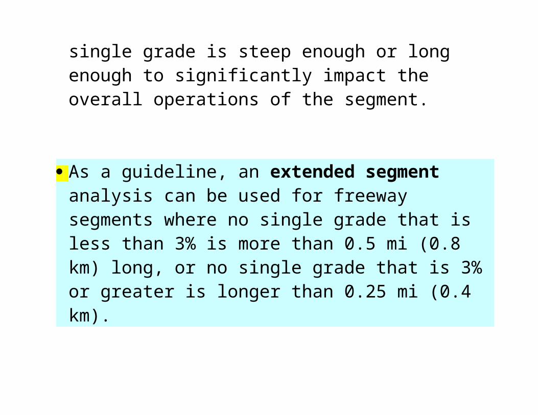
Table 6.7 Passenger Car Equivalents (PCEs) for Extended Freeway Segments
Factor Type of TerrainLevel Rolling Mountainous
ET (trucks and buses) 1.5 2.5 4.5ER (RVs) 1.2 2.0 4.0
From Eq. 6.5:
with PT = 0.15

So,
pc/h/ln
From Fig. 6.2:
For a flow rate of 1144 and a FFS of 58.5 mi/h yields LOS C.
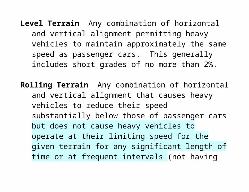
Figure 6.3 Basic Freeway Segment Speed-Flow Curves and Level of Service Criteria.

Or, using 58.5 from Fig. 6.2.
Density from Eq. 6.6.
pc/mi/ln
From Table 6.1, it can be seen that this corresponds to LOS C.
(18.0 [max density for LOS B] < 19.56 < 26.0 [max density for LOS C]).
Thus, this freeway segment operates at level of service C.

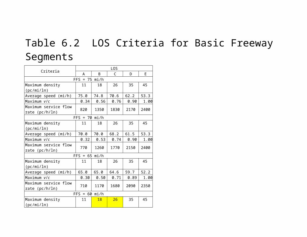
Table 6.2 LOS Criteria for Basic Freeway SegmentsCriteria
LOSA B C D E
FFS = 75 mi/hMaximum density (pc/mi/ln) 11 18 26 35 45Average speed (mi/h) 75.0 74.8 70.6 62.2 53.3Maximum v/c 0.34 0.56 0.76 0.90 1.00Maximum service flow rate (pc/h/ln)
820 1350 1830 2170 2400
FFS = 70 mi/hMaximum density (pc/mi/ln) 11 18 26 35 45Average speed (mi/h) 70.0 70.0 68.2 61.5 53.3Maximum v/c 0.32 0.53 0.74 0.90 1.00Maximum service flow rate (pc/h/ln)
770 1260 1770 2150 2400
FFS = 65 mi/hMaximum density (pc/mi/ln) 11 18 26 35 45Average speed (mi/h) 65.0 65.0 64.6 59.7 52.2Maximum v/c 0.30 0.50 0.71 0.89 1.00Maximum service flow rate (pc/h/ln)
710 1170 1680 2090 2350
FFS = 60 mi/hMaximum density (pc/mi/ln) 11 18 26 35 45Average speed (mi/h) 60.0 60.0 60.0 57.6 51.1Maximum v/c 0.29 0.47 0.68 0.88 1.00Maximum service flow rate (pc/h/ln)
660 1080 1560 2020 2300
FFS = 55 mi/hMaximum density (pc/mi/ln) 11 18 26 35 45Average speed (mi/h) 55.0 55.0 55.0 54.7 50.0Maximum v/c 0.27 0.44 0.64 0.85 1.00Maximum service flow rate (pc/h/ln)
600 990 1430 1910 2250

EXAMPLE 6.2
Consider the freeway and traffic conditions in Example 6.1. At some point further along the roadway there is a 6% upgrade that is 1.5 mi long. All other characteristics are the same as in Example 6.1. What is the level of service of this portion of the roadway and how many vehicles can be added before the roadway reaches capacity (assuming that the proportion of vehicle types and the peak-hour factor remain constant)?

SOLUTION
To determine the LOS of this segment of the freeway, we note
that all adjustment factors are the same as those in Example 6.1
except fHV, which must now be determined using an
equivalency factor, ET, drawn from the specific upgrade tables
(in this case Table 6.8).
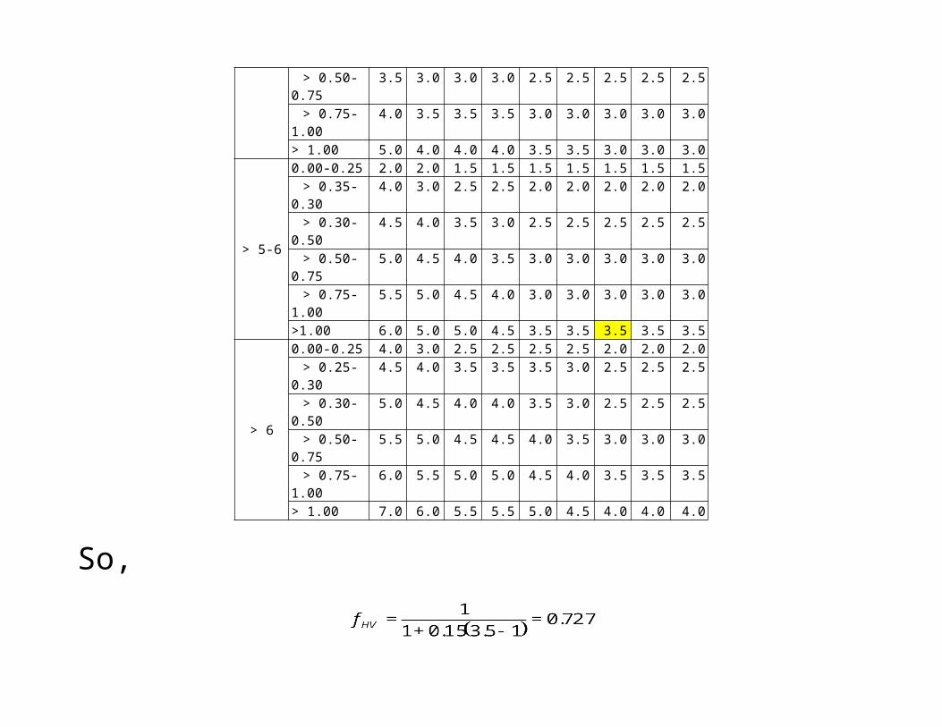
From Table 6.8, with 15% large trucks and buses, ET = 3.5.

Table 6.8 Passenger Car Equivalents (PCEs) for Trucks and Buses on Specific Upgrades
Upgrade(%)
Length(mi)
ET
Percentage of Trucks and Buses2 4 5 6 8 10 15 20 25
< 2 All 1.5 1.5 1.5 1.5 1.5 1.5 1.5 1.5 1.5
2-3
0.0-0.25 1.5 1.5 1.5 1.5 1.5 1.5 1.5 1.5 1.5> 0.25-0.50 1.5 1.5 1.5 1.5 1.5 1.5 1.5 1.5 1.5> 0.50-0.75 1.5 1.5 1.5 1.5 1.5 1.5 1.5 1.5 1.5> 0.75-1.00 2.0 2.0 2.0 2.0 1.5 1.5 1.5 1.5 1.5> 1.00-1.50 2.5 2.5 2.5 2.5 2.0 2.0 2.0 2.0 2.0> 1.50 3.0 3.0 2.5 2.5 2.0 2.0 2.0 2.0 2.0
> 3-4
0.00-0.25 1.5 1.5 1.5 1.5 1.5 1.5 1.5 1.5 1.5> 0.25-0.50 2.0 2.0 2.0 2.0 2.0 2.0 1.5 1.5 1.5> 0.50-0.75 2.5 2.5 2.0 2.0 2.0 2.0 2.0 2.0 2.0> 0.75-1.00 3.0 3.0 2.5 2.5 2.5 2.5 2.0 2.0 2.0> 1.00-1.50 3.5 3.5 3.0 3.0 3.0 3.0 2.5 2.5 2.5> 1.50 4.0 3.5 3.0 3.0 3.0 3.0 2.5 2.5 2.5
> 4-5
0.0-0.25 1.5 1.5 1.5 1.5 1.5 1.5 1.5 1.5 1.5> 0.25-0.50 3.0 2.5 2.5 2.5 2.0 2.0 2.0 2.0 2.0> 0.50-0.75 3.5 3.0 3.0 3.0 2.5 2.5 2.5 2.5 2.5> 0.75-1.00 4.0 3.5 3.5 3.5 3.0 3.0 3.0 3.0 3.0> 1.00 5.0 4.0 4.0 4.0 3.5 3.5 3.0 3.0 3.0
> 5-6
0.00-0.25 2.0 2.0 1.5 1.5 1.5 1.5 1.5 1.5 1.5> 0.35-0.30 4.0 3.0 2.5 2.5 2.0 2.0 2.0 2.0 2.0> 0.30-0.50 4.5 4.0 3.5 3.0 2.5 2.5 2.5 2.5 2.5> 0.50-0.75 5.0 4.5 4.0 3.5 3.0 3.0 3.0 3.0 3.0> 0.75-1.00 5.5 5.0 4.5 4.0 3.0 3.0 3.0 3.0 3.0>1.00 6.0 5.0 5.0 4.5 3.5 3.5 3.5 3.5 3.5
> 6
0.00-0.25 4.0 3.0 2.5 2.5 2.5 2.5 2.0 2.0 2.0> 0.25-0.30 4.5 4.0 3.5 3.5 3.5 3.0 2.5 2.5 2.5> 0.30-0.50 5.0 4.5 4.0 4.0 3.5 3.0 2.5 2.5 2.5> 0.50-0.75 5.5 5.0 4.5 4.5 4.0 3.5 3.0 3.0 3.0> 0.75-1.00 6.0 5.5 5.0 5.0 4.5 4.0 3.5 3.5 3.5> 1.00 7.0 6.0 5.5 5.5 5.0 4.5 4.0 4.0 4.0

So,
(down from 0.816 in Example 6.1)
pc/h/ln (up from 1144 in Example 6.1)
The average passenger car speed remains 58.5 mi/h (still on the flat portion of the curve in Fig. 6.3), thus
pc/mi/ln (19.56 in Example 6.1)
which still gives LOS C from Fig 6.3 and Table 6.1.

Figure 6.4 Basic Freeway Segment Speed-Flow Curves and Level of Service Criteria.

To determine how many vehicles can be added before capacity is reached, the hourly volume at capacity must be computed.
Recall that capacity corresponds to a volume-to-capacity ratio of 1.0 (the threshold between LOS E and LOS F).

Table 6.3 LOS Criteria for Basic Freeway SegmentsCriteria
LOSA B C D E
FFS = 75 mi/hMaximum density (pc/mi/ln) 11 18 26 35 45Average speed (mi/h) 75.0 74.8 70.6 62.2 53.3Maximum v/c 0.34 0.56 0.76 0.90 1.00Maximum service flow rate (pc/h/ln)
820 1350 1830 2170 2400
FFS = 70 mi/hMaximum density (pc/mi/ln) 11 18 26 35 45Average speed (mi/h) 70.0 70.0 68.2 61.5 53.3Maximum v/c 0.32 0.53 0.74 0.90 1.00Maximum service flow rate (pc/h/ln)
770 1260 1770 2150 2400
FFS = 65 mi/hMaximum density (pc/mi/ln) 11 18 26 35 45Average speed (mi/h) 65.0 65.0 64.6 59.7 52.2Maximum v/c 0.30 0.50 0.71 0.89 1.00Maximum service flow rate (pc/h/ln)
710 1170 1680 2090 2350
FFS = 60 mi/hMaximum density (pc/mi/ln) 11 18 26 35 45Average speed (mi/h) 60.0 60.0 60.0 57.6 51.1Maximum v/c 0.29 0.47 0.68 0.88 1.00Maximum service flow rate (pc/h/ln)
660 1080 1560 2020 2300
FFS = 55 mi/hMaximum density (pc/mi/ln) 11 18 26 35 45Average speed (mi/h) 55.0 55.0 55.0 54.7 50.0Maximum v/c 0.27 0.44 0.64 0.85 1.00Maximum service flow rate (pc/h/ln)
600 990 1430 1910 2250

The maximum service flow rate that can be accommodated for a free-flow-speed of 58.5 mi/h is 2285 pc/h/ln (by linear interpolation of Table 6.1).
At 55mi/h, 2250; at 60mi/h, 2300. Interpolating: X/50 = 3.5/5 which gives X=35, so 2250+35=2285.

Eq. 6.6 is used to solve for the hourly volume based upon the maximum service flow rate,
which gives V = 3917 veh/h.
This means that about 1717 vehicles (3917 – 2200) can be added to the peak hour before capacity is reached.
Note that the assumption that the peak-hour factor would remain constant as the roadway approaches capacity is not very realistic. In practice it is observed that, as a roadway approaches capacity, the PHF gets closer to 1.

CE 361In-Class Design Problem #6: Freeway level of service
A four-lane urban freeway is located on rolling terrain, has 12-ft lanes, no lateral obstructions within 6 ft of the pavement edges, and an interchange every 2 miles. The traffic stream consists of cars, buses, and large trucks (no recreational vehicles). A weekday directional peak-hour volume of 1800 vehicles (familiar users) is observed with 700 arriving in the most congested 15-min period. If a level of service no worse than D is desired, determine the maximum number of large trucks and buses that can be present in the peak-hour traffic stream and the traffic density.

6.4 MULTILANE HIGHWAYS
Similar to freeways in most respects, except:
vehicles may enter or leave the roadway at at-grade intersections and driveways,
multilane highways may or may not be divided (by a barrier or median separating opposing directions of flow), whereas freeways are always divided,
traffic signals may be present,
design standards (such as design speeds) are sometimes lower than those for freeways, and
the visual setting and development along multilane highways is usually more distracting to drivers than in the freeway case.
Multilane highways are usually four or six lanes (both directions),
have posted speed limits between 40 and 60 mi/h (65 and 100 km/h), and
can have physical medians, medians that are two-way left-turn-lanes (TWLTLs), or opposing directional volumes that may not be divided by a median at all.

Procedure will be valid only for sections of highway that are not significantly influenced by large queue formations and dissipations resulting from traffic signals (this is generally taken as having traffic signals spaced 2.0 mi [3.2 km] apart or more),
do not have significant on-street parking,
do not have bus stops with high usage, and
do not have significant pedestrian activity.

Figure 6.5 Example Multilane Highways (divided and undivided)

Table 6.11 LOS Criteria for Multilane Highways
LOSFree-Flow
SpeedCriteria A B C D E
60 mi/h
Maximum density (pc/mi/ln) 11 18 26 35 40Average speed (mi/h) 60.0 60.0 59.4 56.7 55.0Maximum v/c 0.30 0.49 0.70 0.90 1.00Maximum service flow rate (pc/h/ln)
660 1080 1550 1980 2200
55 mi/h
Maximum density (pc/mi/ln) 11 18 26 35 41Average speed (mi/h) 55.0 55.0 54.9 52.9 51.2Maximum v/c 0.29 0.47 0.68 0.88 1.00Maximum service flow rate (pc/h/ln)
600 990 1430 1850 2100
50 mi/h
Maximum density (pc/mi/ln) 11 18 26 35 43Average speed (mi/h) 50.0 50.0 50.0 48.9 47.5Maximum v/c 0.28 0.45 0.65 0.86 1.00Maximum service flow rate (pc/h/ln)
550 900 1300 1710 2000
45 mi/h
Maximum density (pc/mi/ln) 11 18 26 35 45Average speed (mi/h) 45.0 45.0 45.0 44.4 42.2Maximum v/c 0.26 0.43 0.62 0.82 1.00Maximum service flow rate (pc/h/ln)
490 810 1170 1550 1900

Figure 6.6 Multilane Highway Speed-Flow Curves and Level of Service Criteria.

6.4.1 Base Conditions and Capacity
12-ft minimum lane widths,
12-ft minimum total lateral clearance from roadside objects (right shoulder and median) in the travel direction,
only passenger cars in the traffic stream,
no direct access points along the roadway,
a divided highway,
level terrain (no grades greater than 2%),
a driver population of mostly familiar roadway users, and
a free-flow speed of 60 mi/h or more.

As was the case with the freeway level of service analysis, adjustments will have to be made when non-base conditions are encountered.
The capacity, c, for multilane highway segments, in pc/h/ln is given in Table 6.12. From Table 6.11, again note that these capacity values correspond to the maximum service flow rate at LOS E and a v/c of 1.0.

Table 6.12 The Relationship Between Free-Flow Speed and Capacity on Multilane Highway Segments
Free-Flow Speedmi/h Capacity
(pc/h/ln)60 220055 210050 200045 1900

6.4.2 Service Measure
Density is again the service measure for determining level of service for multilane highways.
Note, unlike freeways, the density threshold for LOS E varies by speed for multilane highways, as can be seen in Table 6.11.
The density thresholds for LOS A-D are the same for multilane highways and freeways.

6.4.3 Determining Free-Flow Speed
The FFS for multilane highways is the mean speed of passenger cars operating in flow rates up to 1400 passenger cars per hour per lane (pc/h/ln).
If the FFS is to be estimated rather than measured, the following equation can be used, which accounts for the roadway characteristics of lane width, lateral clearance, the presence (or lack) of a median, and access frequency.
(6.7)

Where:
FFS = estimated free-flow speed in mi/h,
BFFS = estimated free-flow speed, in mi/h, for base conditions,
fLW = adjustment for lane width in mi/h,
fLC = adjustment for lateral clearance in mi/h,
fM = adjustment for median type in mi/h, and
fA = adjustment for the number of access points along the roadway in mi/h.

Base free-flow speed (BFFS):
7mi/h higher than the speed limit for roads posted 40 and 45mi/h
5 mi/h higher than the speed limit for roads posted 50 mi/h and above

6.4.3.1 Lane Width Adjustment
The same lane width adjustment factor values are used for multilane highways as are used for freeways. Thus, Table 6.3 should be used for multilane highways as well.
Table 6.3 Adjustment for Lane Width
Lane Width (ft)
Reduction in Free-Flow Speed, fLW (mi/h)
12 0.011 1.910 6.6

6.4.3.2Lateral Clearance Adjustment
The adjustment factor for potentially restrictive lateral clearances (fLC) is determined first by computing the total lateral clearance, which is defined as,
(6.8)
Where:TLC = total lateral clearance in ft (m),LCR = lateral clearance on the right side of the traveled
lanes to obstructions (retaining walls, utility poles, signs, trees, etc.), and

LCL = lateral clearance on the left side of the traveled lanes to obstructions.
For undivided highways, there is no adjustment for left-side lateral clearance because this is already taken into account in the fM term (LCL = 6 ft in Eq. 6.8).
If an individual lateral clearance (either left or right side) exceeds 6 ft, 6 ft is used in Eq. 6.8.
Highways with TWLTLs are considered to have an LCL equal to 6 ft.
Once Eq. 6.8 is applied, the value for fLC can be determined directly from Table 6.13.

Table 6.13 Adjustment for Lateral Clearance
TotalLateral Clearancea (ft)
Reduction in FFS(mi/h)
Four-Lane Highways
Six-Lane Highways
12 0.0 0.010 0.4 0.48 0.9 0.96 1.3 1.34 1.8 1.72 3.6 2.80 5.4 3.9

6.4.3.3 Median AdjustmentValues for the adjustment factor for median type, fM, are provided in Table 6.14.
Table 6.14 Adjustment for Median Type
Median Type Reduction in FFS
(mi/h) (km/h)Undivided highways 1.6 2.6Divided highways (including TWLTLs) 0.0 0.0

6.4.3.4 Access Frequency AdjustmentThe final adjustment factor in Eq. 6.7 is for the number of access points per mile, fA. Defined to include intersections and driveways (on the right
side of the highway in the direction being considered) that significantly influence traffic flow (no driveways to individual residences or commercial service driveways.
Table 6.15 Adjustment for Access-Point Frequency
Access Points/Mile Reduction in FFS(mi/h)0 0.0
10 2.520 5.030 7.5
40 10.0

6.4.4 Determining Analysis Flow Rate
The analysis flow rate for multilane highways is determined in the same manner as that for freeways, using Eq. 6.3.
There minor difference for multilane highways. An extended segment (general terrain type) analysis can be used for multilane highway segments if:
grades of 3% or less do not extend for more than 1 mi (as opposed to 0.5 mi for freeway) or
any grades greater than 3% do not extend for more than 0.5 mi (as opposed to 0.5 mi for freeway).

6.4.5 Calculating Density and Determining LOS
Same as freeways but slightly different speed-flow curves and level of service criteria are used for multilane highways (see Table 6.11 and Fig. 6.4).
To determine density, average passenger-car speed is found by reading from the y-axis of Fig. 6.4 for the corresponding analysis flow rate (vp) and free-flow speed.

EXAMPLE 6.3
A four-lane undivided highway has 11-ft lanes, with 4-ft shoulders on the right side. There are 7 access points per mile and the posted speed limit is 50 mi/h. What is the estimated free-flow speed?
SOLUTION
Use Eq. 6.7 to arrive at an estimated free-flow-speed.

With:
BFFS = 55 mi/h (assume FFS = posted speed + 5 mi/h)
fLW = 1.9 mi/h (Table 6.3)
Table 6.3 Adjustment for Lane Width
Lane Width (ft)
Reduction in Free-Flow Speed, fLW (mi/h)
12 0.011 1.910 6.6

fLC = 0.4 mi/h (Table 6.13, with TLC = 4 + 6 = 10 from
Eq. 6.8, with LCL = 6 ft because highway undivided)
Table 6.13 Adjustment for Lateral Clearance
TotalLateral Clearancea (ft)
Reduction in FFS(mi/h)
Four-Lane Highways
Six-Lane Highways
12 0.0 0.010 0.4 0.48 0.9 0.96 1.3 1.34 1.8 1.72 3.6 2.80 5.4 3.9

fM = 1.6 mi/h (Table 6.14)
Table 6.14 Adjustment for Median Type
Median Type Reduction in FFS
(mi/h) (km/h)Undivided highways 1.6 2.6Divided highways (including TWLTLs) 0.0 0.0

fA = 1.75 mi/h (Table 6.15, by interpolation, 7 per mile)
Table 6.15 Adjustment for Access-Point Frequency
Access Points/Mile Reduction in FFS(mi/h)0 0.0
10 2.520 5.030 7.5
40 10.0

Substitution gives:
which means that the more restrictive roadway characteristics relative to the base conditions result in a reduced free-flow speed of 5.65 mi/h.

EXAMPLE 6.4
A six-lane divided highway is on rolling terrain with 2 access points per mile and has 10-ft lanes, with a 5-ft shoulder on the right side and a 3-ft shoulder on the left side. The peak-hour factor is 0.80 and the directional peak-hour volume is 3000 vehicles per hour. There are 6% large trucks, 2% buses, and 2% recreational vehicles. A significant percentage of non-familiar roadway users are in the traffic stream (the driver population adjustment factor is estimated as 0.95). No speed studies are available, but the posted speed limit is 55 mi/h. Determine the level of service.

SOLUTION
We begin by determining the FFS by applying Eq. 6.7,
With:
BFFS = 60 mi/h (assume FFS = posted speed + 5 mi/h)
fLW = 6.6 mi/h (Table 6.3)
Table 6.3 Adjustment for Lane Width
Lane Width (ft)
Reduction in Free-Flow Speed, fLW (mi/h)
12 0.011 1.910 6.6

fLC = 0.9 mi/h (Table 6.13, TLC = 5 + 3 = 8 from Eq. 6.8)
Table 6.13 Adjustment for Lateral Clearance
TotalLateral Clearancea (ft)
Reduction in FFS(mi/h)
Four-Lane Highways
Six-Lane Highways
12 0.0 0.010 0.4 0.48 0.9 0.96 1.3 1.34 1.8 1.72 3.6 2.8

0 5.4 3.9
fM = 0.0 mi/h (Table 6.14)
Table 6.14 Adjustment for Median Type
Median Type Reduction in FFS
(mi/h) (km/h)Undivided highways 1.6 2.6Divided highways (including TWLTLs) 0.0 0.0
fA = 0.5 mi/h (Table 6.15, by interpolation, 2 Access
points/mi)
Table 6.15 Adjustment for Access-Point Frequency
Access Points/Mile Reduction in FFS(mi/h)0 0.0
10 2.520 5.030 7.5
40 10.0
Substitution gives,

Determine the analysis flow rate using Eq. 6.3,
With:
V = 3000 veh/h (given)
N = 3 (given)
PHF = 0.8 (given)
ET = 2.5 (Table 6.7)

ER = 2.0 (Table 6.7)
Table 6.7 Passenger Car Equivalents (PCEs) for Extended Freeway Segments
Factor Type of TerrainLevel Rolling Mountainous
ET (trucks and buses) 1.5 2.5 4.5ER (RVs) 1.2 2.0 4.0
fp = 0.95 (given)
From Eq. 6.5,

Substitution gives,
Using Fig. 6.4, construct a speed-flow curve for 52 mi/h FFS (drawing it parallel to the curves for 55 and 50 mi/h) with 1500.3 pc/h/ln flow rate gives LOS D.
Figure 6.7 Multilane Highway Speed-Flow Curves and Level of Service Criteria.

EXAMPLE 6.5
A local manufacturer wishes to open a factory near the segment of highway described in Example 6.4. How many large trucks can be added to the peak-hour directional volume before capacity is reached? (Assume only trucks and buses are added and that the PHF remains constant).

SOLUTION
Note that the FFS will remain unchanged at 52 mi/h.
Table 6.11 shows:
capacity for FFS = 55 mi/h is 2100 pc/h/ln
for FFS = 50 mi/h is 2000 pc/h/ln,
linear interpolation gives a capacity of 2040 pc/h/ln
at a FFS of 52 mi/h.
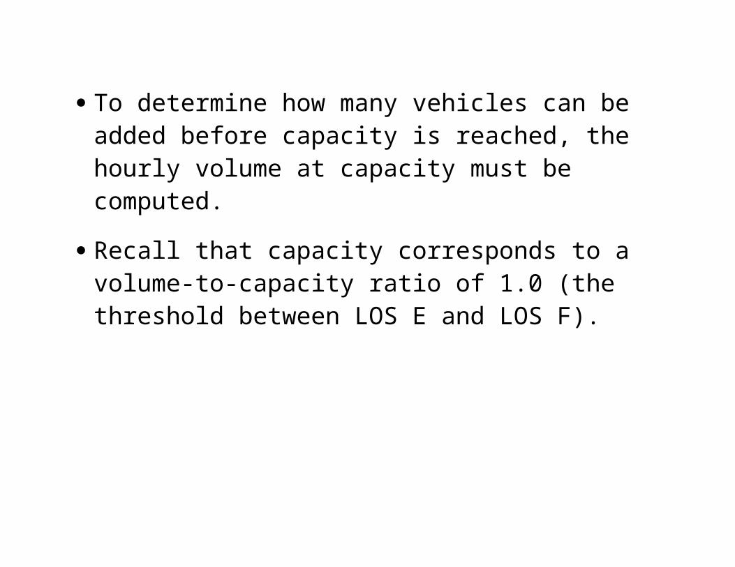
Table 6.11 LOS Criteria for Multilane Highways
LOSFree-Flow
SpeedCriteria A B C D E
60 mi/h
Maximum density (pc/mi/ln) 11 18 26 35 40Average speed (mi/h) 60.0 60.0 59.4 56.7 55.0Maximum v/c 0.30 0.49 0.70 0.90 1.00Maximum service flow rate (pc/h/ln)
660 1080 1550 1980 2200
55 mi/h
Maximum density (pc/mi/ln) 11 18 26 35 41Average speed (mi/h) 55.0 55.0 54.9 52.9 51.2Maximum v/c 0.29 0.47 0.68 0.88 1.00Maximum service flow rate (pc/h/ln)
600 990 1430 1850 2100
50 mi/h
Maximum density (pc/mi/ln) 11 18 26 35 43Average speed (mi/h) 50.0 50.0 50.0 48.9 47.5Maximum v/c 0.28 0.45 0.65 0.86 1.00Maximum service flow rate (pc/h/ln)
550 900 1300 1710 2000
45 mi/h
Maximum density (pc/mi/ln) 11 18 26 35 45Average speed (mi/h) 45.0 45.0 45.0 44.4 42.2Maximum v/c 0.26 0.43 0.62 0.82 1.00Maximum service flow rate (pc/h/ln)
490 810 1170 1550 1900

The current number of large trucks and buses in the peak-hour traffic stream is 240 (0.08´3000) and the current number of recreational vehicles is 60 (0.02´3000).
Let Vnt be the number of new trucks so the combination of Eqs. 6.3 and 6.5
(6.5)

gives,
With:
vp = 2040 pc/h/ln,
V = 3000 veh/h (Example 6.4),
N = 3 (Example 6.4),
PHF = 0.8 (Example 6.4),
ET = 2.5 (Example 6.4),

ER = 2.0 (Example 6.4), and
fp = 0.95 (Example 6.4).
which gives (≈ 492), which is the number of trucks that can be added to the peak hour before capacity is reached.

In-Class Design Problem #7:Multilane highway level of service
A new four-lane undivided multilane highway is being planned with 11-ft lanes, 4-ft right-hand shoulder, and a 50 mi/h speed limit. One 3% downgrade is 4.5 mi long and there will be 4 access points per mile. The peak-hour directional volume along this grade is estimated to consist of 1800 passenger cars, 130 large trucks, 30 buses, and 40 recreational vehicles. The driver population adjustment factor is estimated to be 0.90. If the peak-hour factor is 0.85, what is the level of service of this highway segment?

6.5 TWO-LANE HIGHWAYS
Pages 200 to 211 Two classes:
Class I (motorists expect high speed) and Class II (less of a high-speed expectation
Level of service measured by average travel speed (ATS) or,
Percent time spent following (PTSF)
See text for additional information on procedures etc.

6.6 DESIGN TRAFFIC VOLUMES
How determine number of lanes to provide?
Select a design-hourly volume
Problem:
Variability in traffic volumes by time of day, day of week, time of year, and type of roadway.

Per
cent
of D
aily
Tra
ffic
Time of Day
Intracity Route
-
2.0
4.0
6.0
8.0
10.0
12:00 AM 6:00 AM 12:00 PM 6:00 PM 12:00 AM
Intercity Route
-
2.0
4.0
6.0
8.0
10.0
12:00 AM 6:00 AM 12:00 PM 6:00 PM 12:00 AM
Figure 6.8. Examples of hourly and daily variation

60
70
80
90
100
110
120
130
140
150
Jan. Feb. Mar. Apr. May. Jun. Jul. Aug. Sep. Oct. Nov. Dec.
Month
Mo
nth
ly A
vera
ge
Dai
ly T
raff
ic a
s P
erce
nt
of
AA
DT
AADT
Figure 6.9 Example of Monthly Traffic Volume Variations for Business and Recreational Access Route

Solution:
Work with percentages of the annual average daily traffic, AADT (in units of vehicles per day and computed as the total yearly traffic volume divided by the number of days in the year).
Convert AADT into Design Hourly Volume (DHV)

Figure 6.10 Highest 100 Hourly Volumes Over a One-year Period for a Typical Roadway.

Design practice in the United States uses a design hourly volume (DHV) that is between the 10th and 50th highest volume hour of the year.
Most common hourly volume used for roadway design is the 30th highest hourly volume of the year.
In practice, the K-factor is used to convert annual average daily traffic (AADT) to the 30th highest hourly volume. K is defined as
(6.15)

Where:
K = a factor used to convert annual average daily traffic to a specified annual hourly volume,
DHV = design hourly volume (typically, the 30th highest annual hourly volume), and
AADT = the roadway’s annual average daily traffic.

For freeways and multilane highways, interest is in directional traffic flows.
Need a factor is needed to reflect the proportion of peak-hour traffic volume traveling in the peak direction.
Denoted as D to get the directional design-hour volume (DDHV) by application of
(6.16)
Where:
DDHV = directional design-hour volume,
D = directional distribution factor to reflect the proportion of peak-hour traffic volume traveling in the peak direction, and

EXAMPLE 6.8
A freeway is to be designed as a passenger-car-only facility for an AADT of 35,000 vehicles per day. It is estimated that the freeway will have a free-flow speed of 70 mi/h. The design will be for commuters and the peak-hour factor is estimated to be 0.85 with 65% of the peak-hour traffic traveling in the peak direction. Assuming that Fig. 6.7 applies, determine the number of 12-ft (3.6-m) lanes required (assuming no lateral obstructions) to provide at least LOS C using the highest annual hourly volume and the 30th highest annual hourly volume.

SOLUTIONBy inspection of Fig. 6.7, the highest annual hourly volume has K1 = 0.148.

So,DDHV = K1 ´ D ´ AADT
= 0.148 ´ 0.65 ´ 35,000 = 3367 veh/h
At LOS C for a FFS of 70 mi/h. From Table 6.1, we see that this value is 1770 pc/h/ln.

Table 6.4 LOS Criteria for Basic Freeway SegmentsCriteria
LOSA B C D E
FFS = 75 mi/hMaximum density (pc/mi/ln) 11 18 26 35 45Average speed (mi/h) 75.0 74.8 70.6 62.2 53.3Maximum v/c 0.34 0.56 0.76 0.90 1.00Maximum service flow rate (pc/h/ln)
820 1350 1830 2170 2400
FFS = 70 mi/hMaximum density (pc/mi/ln) 11 18 26 35 45Average speed (mi/h) 70.0 70.0 68.2 61.5 53.3Maximum v/c 0.32 0.53 0.74 0.90 1.00Maximum service flow rate (pc/h/ln)
770 1260 1770 2150 2400
FFS = 65 mi/hMaximum density (pc/mi/ln) 11 18 26 35 45Average speed (mi/h) 65.0 65.0 64.6 59.7 52.2Maximum v/c 0.30 0.50 0.71 0.89 1.00Maximum service flow rate (pc/h/ln)
710 1170 1680 2090 2350
FFS = 60 mi/hMaximum density (pc/mi/ln) 11 18 26 35 45Average speed (mi/h) 60.0 60.0 60.0 57.6 51.1Maximum v/c 0.29 0.47 0.68 0.88 1.00Maximum service flow rate (pc/h/ln)
660 1080 1560 2020 2300
FFS = 55 mi/hMaximum density (pc/mi/ln) 11 18 26 35 45Average speed (mi/h) 55.0 55.0 55.0 54.7 50.0Maximum v/c 0.27 0.44 0.64 0.85 1.00Maximum service flow rate (pc/h/ln)
600 990 1430 1910 2250

.Use Eq. 6.3 to find vp, based on an assumed number of lanes.
Compare vp to the maximum service flow rate of 1770 will determine whether we have an adequate number of lanes.
With V = DDHV, and assuming a four-lane freeway, Eq. 6.3 gives,
pc/h/ln
With:
fLW = 1.0 (Table 6.2; 12-ft lanes, no obstructions)
fHV = 1.0 (no heavy vehicles)
fp = 1.0 (commuters)
Value is higher than 1770, so we need to provide more lanes. The calculation is repeated, this time with an assumed six-lane freeway.
pc/h/ln
1320.4 < 1770, 3 lanes each direction necessary for LOS C.
For the 30th highest hourly annual volume, Fig. 6.7 gives K30 = K = 0.12, which, when used in Eq. 6.16 gives

DDHV = K ´ D ´ AADT
= 0.12 ´ 0.65 ´ 35,000 = 2730 veh/h

Apply Eq. 6.3, with an assumed four-lane freeway, yields
pc/h/ln
This value is less than 1770, so a four-lane freeway (two lanes each direction) is adequate for this design traffic flow rate.