lens design for manufacture - loughborough university · lens design for manufacture ... metadata...
TRANSCRIPT

Loughborough UniversityInstitutional Repository
Lens design for manufacture
This item was submitted to Loughborough University's Institutional Repositoryby the/an author.
Additional Information:
• A Doctoral Thesis. Submitted in partial fulfilment of the requirementsfor the award of Doctor of Philosophy of Loughborough University.
Metadata Record: https://dspace.lboro.ac.uk/2134/14554
Publisher: c© Richard John Tomlinson
Please cite the published version.

This item was submitted to Loughborough University as a PhD thesis by the author and is made available in the Institutional Repository
(https://dspace.lboro.ac.uk/) under the following Creative Commons Licence conditions.
For the full text of this licence, please go to: http://creativecommons.org/licenses/by-nc-nd/2.5/

! University Library
•• Lo,!ghbprough • Umverslty I
I
- R: AuthorlFiling Title ...... \O'.M·I,.,.J.~$·Q·~·I····· .. ~·9:\&BJ) I
........................................................................................ I
T Class Mark .................................................................... .
Please note that fines are charged on ALL overdue items.
if~iiiillll 11111111111 ~I


Lens Design for Manufacture
by
Richard John Tomlinson
A Doctoral Thesis submitted in partial fulfilment of the requirements for the award of
Doctor of Philosophy
of the Loughborough University
December 2004 ;
Research Supervisor: Dr. J M Coupland Dr. J Petzing
© Richard John Tomlinson

U LoughbOrough Univet'sitV , . Pilkington Library
Date ~~ 2.o0S
Class -r -
Ace ~ . No. oLf03 \9 \3 X,;V

Abstract
Abstract
The manufacture of complete optical systems can be broken down into three
distinct stages; the optical and mechanical design, the production of both optical
and mechanical components and finally their assembly and test. The three stages
must not be taken in isolation if the system is to fulfil its required optical
performance at reasonable cost.
This report looks first at the optical design phase. There are a number of
different optical design computer packages on the market that optimise an optical
system for optical performance. These packages can be used to generate the
maximum manufacturing errors, or tolerances, which are permissible if the
system is to meets its design requirement. There is obviously a close relationship
between the manufacturing tolerances and the cost of the system, and an analysis
of this relationship is presented in this report. There is also an attempt made to
optimise the design of a simple optical system for cost along with optical
performance.
Once the design is complete the production phase begins and this report then
examines the current techniques employed in the manufacture, and testing of
optical components. There are numerous methods available to measure the
surface form generated on optical elements ranging from simple test plates
through to complex interferometers. The majority of these methods require the
element to be removed from the manufacturing environment and are therefore
not in-process techniques that would be the most desirable. The difficulties
surrounding the measurement of aspheric surfaces are also discussed. Another
common theme for the non-contact test techniques is the requirement to have a
test or null plate which can either limit the range of surfaces the designer may
chose from or increase the cost of the optical system as the test surface will first
have to be manufactured. The development of the synthetic aperture
interferometer is presented in this report. This technique provides a non-contact
method of surface form measurement of aspheric surfaces without needing null
or test plates.

Abstract
The final area to be addressed is the assembly and test stage. The current
assembly methods are presented, with the most common industry standard
method being to fully assemble the optical system prior to examining its
performance. Also, a number of active alignment techniques are discussed
including whether the alignment of the individual optical elements is checked,
and if need be adjusted, during the assembly phase. In general these techniques
rely upon the accuracy of manufacture of the mechanical components to facilitate
the optical alignment of the system. Finally a computer aided optical alignment
technique is presented which allows the optical alignment of the system to be
brought within tolerance prior to the cementing in place of an outer casing. This
method circumvents the need for very tight manufacturing tolerances on the
mechanical components and also removes the otherwise labour intensive task of
assembling and disassembling an optical system until the required level of
performance is achieved.
11

Acknowledgements
Acknowledgements
Many thanks to Jeremy Coupland for both his guidance and patience throughout
this project.
Huge thanks to Jon Petzing for all his support and advice.
Thanks to all of the technical and workshop staff without whose assistance many
of the mechanical components would not have been manufactured.
Thanks also to Ben, Emma, Adrian, Anton, Candi, and John for making coming
to work such a pleasure.
Thanks to Mum, Dad, Andy and Leanne for their support.
And finally, thanks to Sarah for everything.
111

Contents
TITLE: Lens Design for Manufacture
Contents
Chapter 1. Introduction 1
1.1 Motivation 2
1.2 Background 2
1.3 The Design Process 3
1.4 Manufacture and Surface Testing 4
1.5 Synthetic Aperture Interferometry 4
1.6 Multi Element Lens Alignment 5
1.7 Outline 5
References 7
Chapter 2. The Lens Design Process 8
2.1 Introduction 9
2.2 Lens Design and Optimisation for Optical Performance 10
2.2.1 Basic Paraxial Optics and Thin Lens Theory 14
2.2.2 Ray Tracing 18
2.2.3 Aberration Theory 19
2.3 Aspheric Optics 23
2.4 Conclusions 25
Figures 26
References 30
Chapter 3. Tolerancing and the Inclusion of a Cost Function
within Optimisation
3.1 Introduction
3.2 The Tolerance Parameters
3.2.1 Introduction to Tolerancing
3.3 Practical Considerations in Lens Design:
The Application of Tolerancing at the Assembly Stage
3.4 Lens Building Example
3.5 The Development of a Cost Model
34
35
35
41
45
49
50
IV

3.6 Existing Optimisation Tools that include Cost
3.7 A Global Cost Model
3.8 Conclusions
Chapter 3. Figures
References
Chapter 4. Optical Element Production and Testing
4.1 Introduction 4.2 The Manufacture of Optical Elements
4.2.1 The Production of Curved Optical Surfaces
4.2.2 The Problems Presented by Aspheric Surfaces
4.3 Surface Form Testing with Particular
Reference to Aspheric Surfaces
4.3.1 Simple Test Plates
4.3.2 Contact Techniques
4.3.3 Interferometric Techniques and other
Optical Non-Contact Techniques
4.4 An Ideal Surface Test System for Aspheric Optics
4.5 Conclusions
Chapter 4. Figures
Chapter 4. References
Chapter 5. Synthetic Aperture Interferometry
5.1 Introduction
5.2 Background to the Synthetic Aperture Technique
5.3 Synthetic Aperture Interferometer Configurations
5.4 Theory
5.5 Implementation and Experiment
5.6 Discussion of Synthetic Aperture Interferometry
and Further Improvements
5.7 Conclusions
Chapter 5. Figures.
Contents
63
64
70
72
82
86
87 87
88
91
92
92
94
95
101
102
103
105
110
111
112
113
115
119
120
121
123
v

References
Chapter 6. Computer-Aided Lens Assembly (CALA)
6.1 Introduction
6.2 The CALA Method
6.3 The Design ofthe Test Set-up
6.4 Experimental Method
6.5 Results
6.6 Discussion and Conclusions
Chapter 6. Figures
References
Chapter 7. Conclusions and Further Work
7.1 Summary
7.2 Conclusions
7.3 Further Work
Chapter 7. Figures
References
Contents
131
132
133
134
138
139
140
143
144
149
150
151
152
154
157
158
Vl

CHAPTER 1
INTRODUCTION
Chapter 1
1

Chapter 1
Chapter 1. Introduction
1.1 Motivation
This thesis is concerned with improving the processes, and reducing the cost of
the manufacture of complex multi-element lens systems. A global view of the
process is presented beginning with the production of a lens specification, and a
discussion of the design and tolerancing stages. The manufacture of optical
components is then addressed with a review of surface form measurement
techniques that are currently employed to check the quality of the optics at this
stage. Particular reference is made to methods that can be applied to the
production and measurement of aspheric surfaces. The final step of the
production process is the build and system test stage where the individual optical
and mechanical components are assembled into the finish saleable product.
These last stages can have a very large impact on the overall cost of the system.
By some estimates the cost of the design and optical manufacture stages can
represent as little as 10% of the overall cost of the system. 1
1.2 Background
This thesis builds upon practical experience of lens building and testing, gained
whilst undertaking a Knowledge Transfer Partnership (KTP) project (formerly
TCS) in the workshops of Van Diemen Ltd of Earl Shilton, Leicestershire, UK.
For the most part Van Diemen was involved with the design and production of
mechanical housings for cinematic lenses. However, the company had a small
production facility for polishing and testing spherical elements.
Initially the author worked in the servIce department where he was soon
responsible for the repair and re-alignment of complex lens systems from a wide
variety of manufacturers. This work illustrated the range of fixing methods that
are used in these types of lenses and the degree of precision afforded by each.
The work also demanded knowledge of the methods used to specify lens
elements so that replacement parts could be manufactured.
2

Chapter 1
Once built, complete lens systems were characterised usmg a variety of
qualitative and quantitative tests and external markings were specified. Working
in this area illustrated the physical consequences of misalignment and the
importance of sound mechanical design.
Returning to Loughborough University, the lens design and manufacture
processes were reconsidered as a whole and a number of key areas were
identified for possible improvements. In the following paragraphs these areas are
briefly discussed before presenting details of this work in the main body of the
thesis.
1.3 The Design Process
Traditionally the lens design process was very labour intensive requiring the
tracing of rays using mechanical calculators and trigonometric tables. Currently,
the vast majority of the design of optical systems is carried out purely on optical
performance until an acceptable solution is reached and then the system is
toleranced to examine the accuracies to which the system must be manufactured
and assembled in order to realise the desired performance criteria. Using this
approach the design may well have to be redesigned if the tolerances are too
restrictive, or, indeeq, are uneconomic to reach in the production environment.
Even if the tolerances are possible at a commercially acceptable cost there is no
guarantee that the most economic solution to the design problem has been found.
Given this, it is clearly desirable to consider the tolerance data and its impact on
cost, along with optical performance criteria, at the optimisation stage of the
design process as this would result in both optically satisfactory and economic
solutions to the design problem. To achieve this aim comprehensive cost models
are required that accurately estimate the costs of manufacture and assembly of
competing designs, and a balance between cost and optical performance
parameters must be reached. The practical implementation of this approach is the
first task considered in this thesis.
3

Chapter 1
1.4 Manufacture and Surface Testing
There are a large number of methods available for the production of optical
elements ranging from the traditional grinding and polishing techniques2 to the
modern Magnetorheological Finishing3 method employing computer controlled
generation of optical surfaces. The lenses must also be tested to ensure that they
have been produced to specification. A number of different test methods are
available to the optical workshop including various interferometric techniques,
and contact and non-contact profilers. Currently, for aspheric surfaces, the
surface form testing is carried out after the lens has been manufactured and is
therefore a consecutive not a concurrent process. In order to reduce the rejection
rate and aid the manufacture of aspheric surfaces, especially by the newer single
point and computer controlled manufacturing techniques, it is desirable to run the
production and test phases concurrently and on the same machine to enable
corrective adjustment of the surface. In most cases current on-machine, in
process measurement techniques are of the profiler type and so only sample
distinct areas rather than the whole surface.
1.5 Synthetic Aperture Interferometry
Surface shape measurement using a novel synthetic aperture interferometer is the
second method introduced and discussed in this thesis. Synthetic Aperture
Interferometry effectively produces a surface shape by knitting together a large
number of measurements that are taken across the entire aperture of the surface
under test. This process has the potential to be included as an in-process, on
machine technique that can be fitted to CNC polishing machines. The method
does not require the use of separate null or test plates and is inherently tolerant of
vibration such as might be experienced in an on-machine application. However,
the technique does use the rear surface of the component as a reference surface
and as such this surface must be calibrated in the same way that any test plate or
null surface. This is a potential disadvantage as in effect every component has its
own un-calibrated reference surface. The technique can be used to measure
aspheric surfaces as well as conventional spherical surfaces.
4

Chapter 1
1.6 Multi Element Lens Alignment
After the component production and measurement phases, the lens system must
be assembled in a manner that satisfies the tolerances placed upon it. At present
the lens systems are generally fully assembled prior to testing. This has obvious
cost and time implications if the system does not meet the required performance
level, and has to be disassembled and rebuilt. A method of Computer-Aided
Lens Assembly (CALA) is presented here in which the individual lens elements
are aligned by following computer instructions. Adjustments which can be made
are decentrations in two orthogonal directions, tilt about two orthogonal axes and
in the axial position (the airspace between the elements). The process continues
iteratively until the system is aligned to within tolerance and low tolerance
mechanical fixturing is then used to secure the elements. The CALA method is
the third manufacturing innovation considered in this thesis.
1.7 Outline
In Chapter 2 of this thesis, the lens design process is examined in detail. Generic
lens specification is presented, followed by a discussion of the optical design
optimisation process. A number of different optimisation methods are outlined
along with a comparison of their relative merits. These different optimisation
tools all have one thing in common in that they optimise the design solely on its
optical performance. The optical theory required by a designer to make the best
use of optical design software is described, beginning with basic paraxial optics
and ray tracing through to a description of the aberrations that degrade the
performance of optical systems.
Chapter 3 describes the tolerancing of optical systems. The parameters to be
toleranced are detailed and computer aided tolerancing is described. A
discussion of how the cost of an optical system is affected by the tolerances
placed upon it, and various models of how these costs change, is presented.
Finally cost parameters are introduced into an optimisation routine, along with
the usual performance criteria, in order to find a more cost effective solution to a
simple optical design problem of a cement doublet lens.
5

Chapter 1
Chapter 4 introduces the vanous methods by which optical elements are
manufactured with particular interest paid to aspheric surfaces generated on
optical glass. The current methods by which the surface form of these lenses is
tested are then discussed. A profile of what would constitute an ideal surface test
method for the production environment is then developed as an aid to the design
of a new type of interferometer.
The design and testing of a new type of interferometer is discussed in Chapter 5.
This technique is similar in concept to Synthetic Aperture Radar where a picture
of the ground is constructed from a large number of smaller images. In this case
there is an analogous interferometric technique, termed Synthetic Aperture
Interferometry,
In Chapter 6, a novel method of lens alignment and build is presented, termed
Computer-Aided Lens Assembly, CALA. This technique employs real and
computer generated ray tracing through the optical system combined with an
optimisation routine that provides corrective displacements for the system.
Chapter 7 concludes the thesis and details the main achievements presented in it.
Areas for further investigation are then highlighted and discussed.
6

Chapter 1
References
1. R.E. Hopkins, "Optical design 1937-1988 ... Where to from here?", Optical
Engineering, Vol. 27, No. 12, pp 1019-1026, (1988).
2. Frank Twyman, "Chapter 3, The Nature of Grinding and Polishing", in Prism
and Lens Making, Adam Hilger, London UK, pp 49-66, (1988).
3. Harvey M. Policove, "Next Generation Optics Manufacturing Technologies",
Advanced Optical Manufacturing and Testing Technology, Proceedings of SPIE
Vol. 4231, pp 8-15, (2000)
7

Chapter 2
CHAPTER 2
THE LENS DESIGN PROCESS
8

Chapter 2
Chapter 2. The Lens Design Process
2.1 Introduction
The lens design process is a very complex and involved task of many steps,
requiring a wide range of skills and experiences. Before the lens design can begin in
earnest, a specification of the desired performance must be drawn up. The
specification contains information concerning the mechanical interface, mounting
system, environmental performance and cost, in addition to the desired optical
performance!. The following is a list of the most common criteria to be considered
before lens design begins; it is by no means an exclusive or exhaustive list, but is
meant as a basic guide.
Focal Length
Zoom Requirement
Aperture size/position
Cost
Mounting System
Image Height
Weight
Field of View
Size
Operating Wavelength
Use of Optical Coatings
Resolution.
Other parameters may be added to this list depending on the specific system
required, and different weightings may be applied to these headings according to
their relative importance to the success of the design. For example, if the designer is
producing a film lens, then the image height must fill the film frame otherwise the
lens will not be useful to the cameraman, so this parameter would have a high
weighting applied to it.
Once the specification has been produced the design of the lens system may begin.
The design process involves finding the optimum performance/cost balance with
respect to the initial specification.
9
Chapter 2
2.2 Lens Design and Optimisation for Optical Performance
The majority of lens design presently carried out is concerned with the optical
performance delivered to the end user. The optimisation routines within the lens
design packages optimise designs by minimizing a parameter known as an error
function (or maximizing a merit function). An error function is a combination of
numerous separate parameters that attempt to describe the performance or quality of
the system within this single value. Error functions vary greatly in type and
complexity and can involve simple generalized models or include large user edited
components that tailor it for a specific use. Error functions can include terms to
limit a design to a particular focal length, f# number, magnification or physical
dimensions such as lens aperture or edge thickness whilst attempting to minimise
wavefront optical path difference (OPD), or spot size at the focal point or at many
points around the field. Each of the separate parameters within the error function is
assigned a weight based on its relative importance, and it is these weights that drive
the optimisation package towards a particular result.
The main lens design software used during the research for this thesis has been the
Sinclair Optics OSLO lens design package2• When constructing an error function
within OSLO, the first choice to be made is what type of error function is the most
appropriate, the RMS (Route Mean Squared) spot size, or the RMS wave front error
type. The method of field and pupil sampling has to be selected, as does the number
of field points. A field point is defined as the coordinate that the ray emanates from,
and so the number of field points defines the minimum number of rays that will be
traced through the system. In general the more field points that are generated the
more accurate the analysis. However, the complexity of the error function is often
limited by the available computing power. Other considerations may be included
within the error function; examples of some included in the OSLO package are
automatic colour correction, and the correction of distortion at full field. A limit
may be put on the distortion and the error function will attempt to abide by this limit
during the optimisation process.
10

Chapter 2
After the generation of the desired lens specification, the next step is the choice of a
suitable starting point for the optimisation. In all but the simplest cases, lens design
packages are incapable of producing acceptable results when starting from a blank
design, without a good starting point and human input from the designer throughout
the optimisation procedure3• In the future, it may be possible to start the
optimisation with flat plates and achieve a viable solution4 by employing sufficient
computing power. However it is not current best practice. At present the designer
must still choose fundamental parameters such as how many surfaces to begin with
and also be able to determine whether the design represents the best possible
solution to the problem. This approach also ignores the fact that there may be an
existing design that with only slight modifications could fulfil the new specification.
Indeed the starting point used for the design is usually taken as an existing design
that has similar optical performance to that required. Optical elements can then be
added and subtracted and other design parameters altered until the new design
specification is realised. Modem lens design packages often include a lens library
specifically to be used as starting points in new lens designs5.
The optimisation variables are now selected. There are many potential variables
including airspace, element thickness, lens curvature, optical glass type and the use
of aspheric curves. The choice of variables greatly affects the progress of the
optimisation, and it is often wise to constrain the optimisation to a limited number of
variables at anyone time. Some of the benefits and drawbacks inherent in the more
commonly employed variables will now be discussed.
The airspace between lenses can be a very useful tool because it is a continuously
variable parameter that can have a large effect on the overall optical performance.
Element thickness, however, is a very different variable. In the majority of designs
it is an ineffective variable and, unless tightly constrained, often results in unfeasibly
thick elements in an attempt to significantly alter the system optical performance6•
Careful limits must also be placed upon the element edge thickness and centre
thickness, in the case of negative elements, if the lens is not to become prohibitively
11

Chapter 2
difficult to manufacture and assemble. This will be discussed further in Chapter 3.
There are still some lenses where element thickness is a useful variable, such as the
older meniscus lenses like Protar and Dagor (where thickness is used to control the
Petzval Curvature and higher order aberrations) 7•
Lens curvature is a powerful variable that has a significant effect on the system
performance for relatively small alterations. This is because it is a combination of
the glass type and curvature that defines the power of the optical element. In most
cases the surface curvature is treated as a continuously variable parameter within the
lens design until the design nears completion. Often these curvatures are then
limited to the curvatures for which the company's optical workshops already have
the tooling and test plates, in order to reduce the cost of the finished design and the
lens is then re-optimised with the new curvatures.
The glass type is an interesting parameter when considered as a variable. For the
purposes of the optimisation, it can be considered as a continuously varying
parameter even though, in reality, the designer (except in exceptional circumstances)
is limited to the glass types already on the market. In this process the optimisation is
allowed to alter the refractive index and dispersion of the glass to reach the highest
level of performance, though they are normally altered in such a way that the design
is limited to non-exotic glass types. Once an acceptable solution has been reached
the theoretical glass types are substituted with their closest equivalent catalogue
glass type and the design is reoptimized with the glass type fixed to produce a high
quality yet manufacturable solution.
The use of aspheric curves within the optimisation can produce very effective results
in terms of optical performance though the optimisation can be very difficult to
constrain, especially as there is a desire to constrain the surface with as few variables
as possible8 since the speed of optimisation is approximately related to the square of
the number of variables involved, and the lens becomes very expensive to
manufacture. Despite this, aspheric elements are increasingly important in modem
12

Chapter 2
lens design and the benefits and manufacturing implications are discussed in detail
elsewhere in this thesis.
Numerous different optimisation techniques are available to the optical designer and
an understanding of their differences and relative strengths is useful when selecting
which method to use. One of the most common optimisation methods is known as
the Damped Least Squares method9• The software will typically alter each of the
specified variables by a small amount, (often the magnitude of the alterations can be
specified by the designer), and then recalculate the error function to determine
whether the performance of the system has been improved. This process will
continue through numerous iterations until the program has reached a suitable end
point or the maximum number of iterations has been reached. There is a simple
landscape analogy!O that can be applied to describe the process, in which the latitude
and longitude are the variables chosen and the elevation represents the value of the
error function. The initial design represents a location on this landscape and the
optimisation routine will move the design through this landscape along a path of
decreasing elevation until a minimum is reached. However, the landscape may have
many depressions and the "local minima" that the program has reached may not be
the best achievable, known as the "global minimum". The minimum that is arrived
at often depends upon the starting position of the design. The design can be shifted
out of local minima by manually introducing a significant change in the variables,
effectively starting the design from a different point in the landscape. Similarly if
part of the design is "frozen" then the design moves away from a local minima and
towards another region of the landscape and hopefully a more acceptable solution.
A more modem method of optimisation is referred to as Simulated Annealing!!.
This is a random search type optimisation method that attempts to find a global
minimum. Before the optimisation routine can begin upper and lower limits must be
placed on all of the variables within the design. The optimisation routine then
randomly selects, with reference to distribution models, values for the variable lens
design parameters within the specified limits and the performance of the resulting
13

Chapter 2
design is analysed. If the lens performs better than the preceding design then it is
accepted. If not, it is rejected. In either case the program continues until the change
in the merit function per step falls below a predetermined level. This method has the
advantage over the Damped Least Squares method in that it jumps from point to
point around the landscape and so does not get caught in local minima. This
behaviour is controlled by a property known within the optimisation routine as
temperature, T, as it is broadly analogous to the temperature in the annealing
process. The level ofT is determined by the lens designer and is lowered throughout
the lens optimisation. At the start of the optimisation, T, has a large value allowing
the optimisation routine to escape from local minima and explore the entire
optimisation region. As the process continues the value of T is slowly lowered until
the optimisation terminates at the global minimum. The rate at which T is reduced is
termed the cooling rate. If the cooling rate is too fast then there is an increasing
possibility that the optimisation will get caught in a local minimum and the
performance of the resulting design will suffer. However, this method takes a great
deal of computing power and is therefore much slower than the Damped Least
Squares method.
Whatever method of optimisation is chosen, with the exception of simulated
annealing, a high degree of optical design ability is still required to produce high
quality results. The designer must choose a suitable start position, select and put
sensible limits on the optimisation variables, and construct an error function that is
tailored to the requirements of the lens specification. The designer must also be able
to determine whether the design has been optimised to its maximum potential or if a
local minima has been found.
2.2.1 Basic Paraxial Optics and Thin Lens Theory
In order to be able to achieve a high performance result, the designer must
understand the optical theory that the lens design packages employ when analysing
the designs. The majority of optical design is based on a process known as ray
14

Chapter 2
tracing, where the progress of a number of rays is traced through an optical system.
However, before ray tracing can be addressed, basic optical calculations need to be
performed and are reviewed here for clarity. The first calculations on any optical
system are generally carried out in the paraxial region of the optical system 12. The
paraxial region is defined as being close to the optical axis, and paraxial rays are
parallel or almost parallel to the optical axis, such that they make only small angles
to it. The ideal optical system can be defined by its cardinal points, consisting of the
focal points, principal planes and nodal pOints13. This simplified optical system can
be thought of as a black box defined between the two principal planes. A diagram
depicting the simplified optical system is provided in Figure 2.1. If the system is
bounded by air on both sides then the first and second nodal points lie on the
principal planes and this case will be assumed for the examples presented here.
Important properties of the system are effective focal length (EFL), defined as the
distance from the rear principal plane to the second focal point; the back focal length
(BFL) is the distance from the rear lens surface to the second focal point, and the
front focal distance (FFL) corresponding to the distance from the first focal point to
the front surface of the optical system. Thin lens theory is employed during the
early stages of optical system design as it enables the designer to quickly estimate
the basic properties of the optical system such as the height and position of an image
formed by the system. The focal length of a single, thin lens with two spherically
curved surfaces can be derived using equation 2.1 sometimes referred to as the
lensmaker's formula I4•
1 1 1 -= (n-l)(---) f RI R2
Where f = focal length of system
n = refractive index of optical glass
RI = radius of curvature of front surface
R2= radius of curvature of rear surface.
2.1
15

Chapter 2
The radius of curvature is considered to be positive when the centre of curvature is
to the right of the vertex of the surface, analogous to a convex surface, and negative
when the centre of curvature is to the left ofthe vertex.
When a lens with a finite thickness is considered, the positions of the focal points
relative to the first and second principal planes have to be considered, and these are
termed fl and f2 respectively. These parameters along with the principal planes and
further dimensions are depicted in Figure 2.2. The property fl can be calculated
using equation 2.215•
Where
(n2 -n,Xn2 -n3 ) t n,n2 R,R2
fl = front focal point, relative to front principal plane
nl = refractive index of medium in front of lens
n2 = refractive index of lens
n3 = refractive index of medium following
t = lens thickness.
And f2 can be calculated by employing equation 2.3.
Where f2 = second focal point, relative to second principal plane
2.2
2.3
The next stage is to calculate the locations of the two principal planes. The location
of the first principal plane is derived using equation 2.4.
2.4
16

Chapter 2
Where r = distance between lens front surface and first principal plane
The location of the second principal plane can be calculated using equation 2.5.
Where s = distance between lens rear surface and second principal plane
In most cases n\ and n3 will be air and so will have the same refractive index and f\
and f2 have the same magnitude and are given the single notation f. Once the
principal planes and focal points of the system have been located, as shown in
Figure 2.2, the image position and size can be calculated. The position of the image
from the second principal plane Si can be calculated using equation 2.6.
111 --+-=- 2.6
So Si f
Where So = the distance from the object to the first principal plane
Sj = the distance from the second principal plane to the image.
In this case distances to the right of the principal plane are considered positive.
The image height is a function of the lateral magnification of the system, m. The
magnification can be found by employing equation 2.7, where x' is the distance from
the second focal point to the image, as defined in Figure 2.2.
x' m=-
f
The image height, h', can then be found using equation 2.8.
2.7
17

h'=h.m
Where h = object height
h'= image height.
Chapter 2
2.8
With the above equations, the basic parameters of the system (the focal length,
image position and size) can be determined. In order to learn more about the
performance of an optical system, rays must be traced through it from object to
image points.
2.2.2 Ray Tracing
The basis of ray tracing is the refraction of light at an optical surface. Snell's law
governs the propagation (If light rays through an optical surface, and is defined in
equation 2.9 and Figure 2.3.
Where Si = angle of incidence
Sr = angle of refraction
nl= refractive index of first medium
n2=refractive index of second medium.
2.9
Figure 2.4 shows how Snell's Law can be applied to calculate the refraction of a
light ray at a single spherically curved surface.
Ray tracing is the basis of optical design analysis. It involves translating rays from
one surface to the next through an optical system starting at the object surface and
terminating at the image plane. The translation stage involves the calculation of the
intercept point on the next surface and then Snell's law, equation 2.9, is applied at
this point of interception.
18

Chapter 2
The detail of ray tracing is beyond the scope of this introduction. However, it is
worth noting if the sine function in Snell's law can be defined to arbitrary precision
by accepting terms of increasing order in a series expansion, equation 2.10.
• (}3 (}s sm() = (}--+-....
3! 5! 2.10
If, for example, the series is cropped to first order, the paraxial formulae that defines
the position and height of the image (equations 2.1-2.8) can be deduced. If the third
order term is taken into account, the primary image aberrations can be defined and
these are outlined in the following section.
2.2.3 Aberration Theory
The aberration characteristics of an optical system can be determined by tracing a
large number of rays through it, and then looking at the amount they deviate from
the paraxial image point. This said, by separating the aberrations into distinct image
flaws, the amount of work required to analyse a system, and the number of rays that
need to be traced, is reduced. Most lens systems currently employ only spherically
polished lens surfaces, so this section refers to spherical surfaces unless otherwise
stated. The primary monochromatic optical aberrations were analysed and defined
by Seidel16 and are often termed Seidel Aberrations. With reference to Figure 2.5
an equation defining the five primary Seidel Aberrations can be seen below17, in
equation 2.11.
Where a(r,e) = wavefront aberration
r,e = the position in polar coordinates
h' = the image height in the exit pupil from the optical axis.
19

Chapter 2
In this case a(r,9) is the wavefront aberration and is defined in the exit pupil as the
deviation from a spherical surface centred on the ideal (paraxial) image point. The
C terms are constants, displayed in the form aCbe where a, band c are the powers of
the h', rand 9 terms respectively. The five aberrations described by this equation
are: r4-spherical aberration; h'r3cos9-coma; h,2rcos29-astigmatism; h,2r -field
curvature, and h,3rcos9-distortion. A discussion of each of these aberrations follows,
describing the causes of each aberration and their effects on the optical performance
of the system.
The first aberration to be considered in detail is spherical aberration, oC40r4, as it is
one of the simplest to understand and analyse. This is the only one of the primary
aberrations that is independent of image height, and its effect is solely dependent on
the position of the ray intercept in the exit pupil. A single double convex lens with
large spherical aberration can be seen in Figure 2.6. The rays passing through the
centre of the lens, the paraxial region, are focused at the paraxial image plane. As
the ray height above the optical axis increases, the rays are focused closer and closer
to the lens as they effectively encounter a larger curvature and therefore a stronger
refractive effect. If the aberration is measured along the optical axis, it is known as
longitudinal spherical aberration. The aberration can also be measured in the lateral
direction to provide the image blur radius. For a specified focal length, the spherical
aberration of a lens will be eight times that of a lens that is only half the diameter.
At a fixed aperture, spherical aberration is dependent upon the object distance and
the curvature of the lens, when considering spherical lenses. This means that by
altering the radius of curvature of both surfaces of the lens, and keeping its focal
length constant, the spherical aberration can be reduced. This process is known as
"bending" the lensl8• Splitting powerful elements in the design into two or more
elements can also reduce spherical aberration. This effectively reduces the angle of
incidence at each surface. It is also noted that an aspheric surface can be free of
spherical aberration as discussed in Section 2.3.
20

Chapter 2
The next aberration to be considered is coma. Coma can be thought of as a change
in the magnification of the lens as a function of aperture, and so it causes the off -
axis rays to arrive at different image points, as can be seen in Figure 2.7 Ca). The
corresponding wavefont diagram is shown in Figure 2. 7 Cb). The aberration is
dependent on the aperture cubed, and image height. The effect of the aberration is to
produce a comet like tail on the image of a point source. Coma is an important
aberration to control because it causes an asymmetric distribution of energy, which
causes images to appear misshapen rather than out of focus, which tends to be the
case with the symmetric aberrations. As in the reduction of spherical aberration,
decreasing the bending of the lens can also reduce coma. Moving the position of the
aperture can reduce coma, as can reducing the diameter of the aperture, though this
causes a loss in light levels through the system. This aberration is an off-axis
problem if the lens is correctly mounted.
Astigmatism occurs when the lens has a different focal position in the sagittal and
tangential planes. For example if the tangential image is closer to the lens than the
sagittal image, then at the tangential image plane, the sagittal image will be
defocused, and at the sagittal image plane the tangential image will be defocused.
Between these positions the image will be blurred. It can be seen that astigmatism is
an off-axis problem because when the image height, h', is zero, the aberration is
zero. In order for astigmatism to be corrected, the tangential and sagittal images
must be made to coincide. Assembling lenses such that the astigmatism in
individual lenses is compensated for, to a degree, by the astigmatism of the system's
other lenses, can reduce overall astigmatism in complex lens systems.
Related to astigmatism is field curvature. The image formed by a positive lens is
naturally curved as can be seen in Figure 2.8. This result is intuitive as the power of
the lens alters as we move off-axis. This curvature causes obvious problems in
applications such as cinematography, where an image has to be put onto a flat film.
However, it is not of great importance when considering viewing systems such as
eyepieces, as the eye compensates for the curvature by adjusting its fOCUS 19• Like
21

Chapter 2
astigmatism, field curvature is a completely off-axis problem. However, unlike
astigmatism, field curvature is an axially symmetric aberration as can be seen from
the lack of a co se term in its definition (see equation 2.11). Field curvature is a
difficult aberration to correct and the approach taken by optical designers is to
minimize the effect of the field curvature inherent in the system. This can achieved
by moving the image plane to a compromise position. Taking the example from
Figure 2.8, the optical designer would move the image plane from its current
position, back towards the lens. However, this would degrade the on-axis
performance. A different approach to minimising the effect of field curvature is to
introduce an element close to the image plane known as a field flattening element2o•
The term used to define the amount of field curvature inherent in an optical system
is the Petzval curvature. The Petzval surface is that which the image would lie on if
the astigmatism of the system were taken as zero.
Distortion is the final monochromatic Seidel aberration and is only present for off
axis image points. It is dependent on the ray height and position, with respect to the
optical axis. Distortion can be thought of as a lateral variation in the magnification
of the lens. Figure 2.9 shows pincushion and barrel distortion of a square grid
pattern. Pincushion distortion is when the magnification increases with distance
from the optical axis. If the magnification decreases with distance form the optical
axis, then the image suffers from barrel distortion. Distortion is generally measured
as a percentage of the calculated paraxial image height, at full field, with 1 to 2%
being generally acceptable for non-measurement systems such as camera lens
systems21•
Axial chromatic aberration, also termed axial colour, is caused by the fact that blue
light is refracted more than red light, if the lens is made with glass that has inherent
positive dispersion. Dispersion relates to the variation of refractive index with
changes in wavelength. Generally the refractive index of optical glass will decrease
with an increase in wavelength causing the red light to be refracted less than the blue
in the same optical element. Therefore, for a positive lens the blue light is imaged
22
Chapter 2
closer to the lens than the red light. This aberration is dependent upon the dispersion
of the different glasses used in an optical system. Specifically chosen combinations
of optical glasses, such as occur in achromatic doublets, are used to correct this
aberration22• In this case a single positive lens is split into two lenses with differing
dispersions. The front element is a positive lens with low dispersion, called the
crown glass. The second element is a negative lens of lower power than the first
lens so the net power of the lens is still positive. This second glass is made of a high
dispersion glass known as flint glass, and corrects most of the chromatic aberration
caused by the first element. Both elements together are known as an achromatic
doublet. The achromatic doublet can also be designed to adopt the opposite form,
where the high dispersion lens constitutes the front element and these are known a
flint leading achromatic doublets23•
Related to axial chromatic aberration is the lateral colour4• If the lens system suffers
from this aberration, then the colour of the light at the image plane varies with image
height off-axis. If again, a simple positive lens after, and separated from, the
aperture stop is considered as an example, the blue light is refracted towards the
optical axis more than the red light. This aberration causes a coloured edge at the
extremes of the field and can be difficult to correct25, especially in wide-angle
applications. This aberration may be corrected by either adopting a lens
construction which is close to (or exactly) symmetric about the aperture stop, or by
achromatising each component individually.
In general it is an impossible task to design a complex real world lens that is
completely free from the effects of all aberrations. It is the task of the lens designer
to minimise and balance the overall combined effect of the individual aberrations, to
produce a solution that meets the specified performance requirements, for as Iowa
cost as possible.
23

Chapter 2
2.3 Aspheric Optics
Traditionally, the vast majority of lens systems consist only of spherical or pIano
optical surfaces. However, as manufacturing technologies have improved, aspheric
optics are becoming more common, especially in low precision applications, though
their use is still rare. The desirability of aspheric components stems from their
ability to reduce image aberrations produced by optical systems. The asphericity of
a surface can defined in a number of different ways including as a conic surface of
revolution26, or as a polynomial function27
• The paraxial focal length is determined
by the spherical radius and the terms of the polynomial are selected to reduce the
aberrations in the system.
Aspheric optics can also be useful in reducing the physical size and weight of lens
systems as they can eliminate the need for the additional elements that are used to
reduce the aberrations inherent in a system. Up until the end of the 19th century,
aspheric optics were generally used to correct for spherical aberration28, and indeed,
a single aspheric surface located close to the aperture stop can in general totally
eliminate spherical aberration of all orders29• As manufacturing technologies have
improved, aspheric lenses can be employed to reduce not only spherical aberration
but astigmatism, distortion, coma and chromatics aberrations. Aspheric mirrors are
employed in the design of high quality reflecting telescopes.
The low precision applications tend to employ aspheric optics that are made from
plastics rather than optical glass, and have been injection moulded as opposed to
polished or diamond turned. These optics generally have small diameters, sub
50mm, and surfaces are only generated to an accuracy of a few microns3o. Higher
precision aspheric components are manufactured by a variety of different means
including polishing with complex tools, diamond turning and Magnetorheolgical
Finishing (MRF), where the surface shaping is carried out by a polishing abrasive
suspended in a magnetic liquid31, the application of which is directed by a magnetic
field. Because of the difficulty in producing accurate aspheric test pieces, the
24

Chapter 2
accurate measurement of surface figure on aspheric components can also
dramatically increase their cost over spherical ones. The manufacture and test of
optical components, and aspheric optics in particular, is discussed in greater detail in
Chapter 4, and a new method of measuring the surface figure aspheric lenses is
presented in Chapter 5.
Given the dramatic benefits that the use of aspheric surfaces can bring to optical
design, the temptation for optical designers to use them can be great. However, it
should be noted that the cost of a single high precision aspheric element can be
greater than that of the several spherical components it is replacing32 and unless
there are pressing size or weight restrictions on the design specification, it may be
better to stay with spherical components.
2.4 Conclusions
Complex lens design is a lengthy and complicated process requiring of the designer
a high degree of optical knowledge and experience if the results are to be acceptable.
The majority of optical design software is based on ray tracing to gain an
appreciation of optical performance. With a few rare exceptions, the design
optimisation and tolerance phases are separate and consecutive. The optimisation is
based solely on optical performance with no method of including relative
manufacturing costs and tolerances when comparing competing design solutions.
The use of aspheric surfaces holds many attractions to the optical designer though
they can still prove prohibitively expensive particularly in high precision
applications. The following chapter contains a discussion of lens tolerancing, and its
impact on complex lens manufacture, combined with an appreciation of how the
manufacturing costs increase as the tolerances are tightened.
25

Chapter 2. Figures
Ray Propagation) Direction
Principal Plane
Lens System
I Second Principal r---~ Plane
Chapter 2
Second Focal /' Point
(='-'-'-'-')'-'-'-'-'-'-'-' Back Focal Length
Effective Focal Length ~----~H------------
Figure 2.1. Basic Optical Layout for a Generalised System
So t E ~ ~
E
~ n3
x' E ~
x -----] h'
nl
\\; Si
First Second Principal Plane Principal Plane
Figure 2.2. Image Height and Position
26

Chapter 2
Incident Ray
Surface Normal
Optical Surface
Refracted Ray
Figure 2.3. SneII's Law Refraction at a Plane Surface
Surface Normal
Curved Surface
Optical Axis
Figure 2.4. Refraction at a Single Curved Surface
27

P
Tangential Axis
Figure 2.5. Off-Axis Ray Geometry
Chapter 2
Principal Ray
Optical Axis
=========II1~~~~~~~f::~ Optical Axis
Figure 2.6. Spherical Aberration.
Figure 2.7 (a). Coma
Paraxial Image Plane
Optical Axis
Paraxial Image Plane
28

1
-1
Figure 2.7 (b) Wavefront Diagram for Coma
Figure 2.8. Field Curvature
Original Grid Pattern Barrel Distortion
Figure 2.9. Distortion
1
Chapter 2
Optical Axis
Flat Image Plane
Pincushion Distortion
29

Chapter 2
References
1. Robert E. Fischer , Biljana Tadic-Galeb, "Chapter 1, Basic Optics and Optical
System Specification" in Optical System Design, SPIE Press & McGraw-HiII, New
York, pp 1-13, (2000).
2. OSLO Optics Software for Layout and Optimisation, Version 6.1, Lamba
Research Corporation, USA, (2001).
3. Robert E. Hopkins, "Optical design 1937-1988 ... Where to from here?", Optical
Engineering, Vol. 27, No. 12, pp 1019-1026, (1988).
4. Milton Laikin, "The future of optical design", Optical Engineering, Vol. 32, No.
8, pp 1729-1730, (1993).
5. Robert E. Fischer , BHjana Tadic-Galeb, "Chapter 9, Basic Optics and Optical
System Specification" in Optical System Design, SPIE Press & McGraw-HiII, New
York, pp 167-180, (2000 .
6. R. R. Shannon, "Chapter 5 Design Optimisation", in The Art and Science of
Optical Design, Cambridge University Press UK, pp 334-353, (1997).
7. Warren J. Smith, "Chapter 2 Automatic Lens Design: Managing the Lens Design
Program", in Modem Lens Design A Resource Manual, McGraw-HiII USA, pp 13-
14, (1992).
8. Scott A. Lemer and Jose M. Sasian, "Optical design with parametrically defined
aspheric surfaces", Applied Optics, Vol. 39, No. 28, pp 5205-5213, (2000).
9. Spencer, "A Flexible Automatic Lens Correction Program", Applied Optics, Vol.
2, pp 1257-1264, (1963).
30

Chapter 2
10. Warren J. Smith, "Chapter 2 Automatic Lens Design: Managing the Lens
Design Program", in Modern Lens Design A Resource Manual, McGraw-Hill USA,
pp 5-7, (1992).
11. Lambda Research Corporation, "Chapter 8 Optimisation", in OSLO Optics
Reference Version 6.1, pp 189-216, (2001).
12. John Blackwell, Shane Thornton. "Chapter 1 Basic Optics", in Mastering Optics,
McGraw-Hill USE, pp 1-34, (1996).
13. Warren J. Smith, "Chapter 2 Image Formation (First Order Optics)", in Modern
Optical Engineering 3rd Edition, McGraw-Hill USA, pp 21-59, (2000).
14. E. Hecht, "Chapter 5 Geometrical Optics", in Optics 3rd Edition, Addison
Wesley, USA, pp 148-246, (1998).
15. Frank L. Pedrotti, Leno S. Pedrotti, "Chapter 4 Matrix Methods in Paraxial
Optics", in Introduction to Optics 2nd Edition, Prentice Hall USA, 62-86, (1996).
16. Max Born, Emil Wolf, "Chapter 5 Geometrical Theory of Aberrations", in
Principles of Optics: Electromagnetic theory of propagation interference and
diffraction of light 6th Edition, Cambridge University Press, pp 203-230, (1997).
17. Frank L. Pedrotti, Leno S. Pedrotti, "Chapter 5 Aberration Theory", in
Introduction to Optics 2nd Edition, Prentice Hall USA, 87-107, (1996).
18. A.E.Conrady, "Chapter 2, Spherical Aberration", in Applied Optics and Optical
Design Part One, Dover Publications Inc, New York, pp 63-66, (1957).
31

Chapter 2
19. Bruce Walker, "Chapter 5, Optical design with OSLO MG" m Optical
Engineering Fundamentals, McGraw Hill, New York, pp 116, (1995).
20. Hecht, "Chapter 6, More on Geometrical Optics", in Optics 3rd Edition,
Addison-Wesley, USA, pp 267-269, (1998).
21. Bruce Walker, "Chapter 6, Primary Lens Aberrations" in Optical Engineering
Fundamentals, McGraw Hill, New York, pp 138, (1995).
22. Leo Levi, "Chapter 9, Lenses and Curved Mirrors", in Applied Optics Volume 1
A Guide to Optical System Design, John Wiley & Sons Inc. New York, pp 410-411,
(1968).
23. Abraham Szulc, "Improved solution for the cemented doublet", Applied Optics,
Vol. 35, No. 19, pp 3548-3557, (1996).
24. A.E.Conrady, "Chapter 4, Chromatic Aberration", in Applied Optics and Optical
Design Part One, Dover Publications Inc, New York, pp 147-150, (1957).
25. Warren J. Smith, "Chapter 5, Review of Specific Geometrical Aberrations", in
Modem Optical Engineering 3rd Edition, McGraw-Hill USA, pp 90-91, (2000).
26. Daniel Malacara, "Appendix 1, An Optical Surface and its Characteristics", in
Optical Shop Testing 2nd Edition, John Wiley & Sons Inc, New York, pp 743-745,
(1992).
27. Ding-Quiang Su, Ya-Nan Wang, "Some ideas about representations of aspheric
optical surfaces", Applied Optics, Vol. 24, No. 3, pp 323-326, (1985).
32
Chapter 2
28. E. Heynacher, "Aspheric Optics: How are they made and why are they needed?",
Phys. Technol., Vol. 10, p 124-139, (1979).
29. R. R. Shannon, "Chapter 7 Design Examples", in The Art and Science of Optical
Design, Cambridge University Press UK, pp 388-602, (1997).
30. K. Becker, B. Dorband, R. Locher, M. Schmidt, "Aspheric Optics at Different
Quality Levels and Functional Need", EUROPTO Conference on Optical
Fabrication and Testing, Proc. ofSPIE, Vol. 3739, pp 22-33, (1999).
3l. Harvey M. Pollicove, "Next Generation Optics Manufacturing Technologies",
Advanced Optical Manufacturing and Testing Technology, Proc. of SPIE, Vol.
4231, pp 8-15, (2000).
32. Warren J. Smith, "Chapter 12 The Design of Optical Systems: General", in
Modern Optical Engineering 3rd Edition, McGraw-Hill USA, pp 393-438, (2000).
33

Chapter 3
CHAPTER 3
TOLERANCING AND THE INCLUSION OF A COST
FUNCTION WITHIN OPTIMISATION
34
Chapter 3
Chapter 3. Tolerancing and the Inclusion of a Cost Function within Optimisation
3.1 Introduction
As discussed in Chapter 2, the traditional approach to optimisation is to complete the
lens design on the grounds of optical performance before examining its production
tolerances and inherent costs. Tolerancing is the technique of calculating and
distributing the manufacturing and assembly errors throughout the optical system, to
ensure that the system will perform to the required standard after it has been
manufactured. It is usually the case that it is the tolerances that are placed upon an
optical design that greatly affect its cost of manufacture. Clearly, the need to repeat
the design process if the manufacturing costs exceed permissible levels is an
inefficient and costly process in itself. With the minimisation of all costs such an
integral part of the make up of any successful business, it would be very useful to
have an element of cost included within the lens design optimisation function.
Crude cost controls do exist, such as limiting the curvatures within the design to
those for which the company already owns test plates, and not allowing the design to
include the more exotic and expensive glass types. However, any workable and
useful cost function would have to be far more complex including such elements as
edge to centre thickness ratio, curvature to centre thickness ratio, an appreciation of
the relative difficulties of generating the curves based on the available
manufacturing set up, glass type, the radius of curvature, the lens centre thickness,
lens diameter, and of course, the associated production tolerances which have such a
large effect on the final cost. These are discussed in the following section.
3.2 The Tolerance Parameters
Before discussing how tolerancing is carried out and subsequently implemented into
the manufacturing process, it is useful to introduce the parameters that are toleranced
and, in some cases, the conventions governing how these tolerances are expressed.
A useful place to begin is the standard tolerances specified within ISO 101101, a
35

Chapter 3
section of which is displayed as Table 3.1. These are the default tolerances that are
to be used if none are specified on a drawing. A typical production drawing for an
optical component is reproduced as Figure 3.1, showing many of the tolerances that
will be discussed in this section. Note that the tolerances vary as the diameter of the
lens alters, even though they are designated for the same nominal level of precision.
The tolerance parameters specified in ISO 10110 will now be discussed, with
reference to the lens drawing in Figure 3.1, in order to show how each of the
tolerances are expressed and specified. The dimensional tolerances, such as
diameter and centre thickness, are self-explanatory and appear in all engineering
applications in some form. The width of the protective chamfer, ground around the
edge of the optical element, is generally pertinent only to optical applications, due to
the inherent brittleness of the materials, and it is employed to reduce the likelihood
of edge damage when the lens is handled during the production and assembly stages.
Maximum dimension of part (mm) Property Up to 10 Over 10 Over 30 Over lOO
Up to 30 ~to 100 Up to 300
Edge length, diameter ±0.2 ±0.5 ± 1.0 ±1.S (mm)
Thickness (mm) ±O.l ±0.2 ±0.4 ±0.8
Angle deviation of ±30' ±30' ±30' ±30' prisms and plate
Width ofprotcctive 0.1-0.3 0.2-0.5 0.3-0.8 0.5 -1.6 cbamfer(mm)
Stress birefiingence 0120 0120 - -(nm/cm)
Bubbles and l13xO.16 1I5xO.25 1I5xOA lISxO.63 inclusions
Inhomogeneity and 211;1 211;1 - -striae
Surface form 3/5(1) 3/10(2) 3/10(2) 3110(2) tolerances 30 mm test 60 mm tcst
diameter diameter
Centcring tolerances 4130' 4120' 4110' 4110'
Surface imperfection 513xO.16 515xO.25 SISxO.4 51SxO.63 tolerances
Table 3.1. ISO 10110 Tolerances.
36

Chapter 3
The following three tolerances to be discussed all appear in the Material
Specification section of the tolerances, as they are uniquely linked to the quality of
glass that the lens is made from. The bubbles and inclusions tolerance2 defines how
many, and what size defects can be present within the glass that the lens is made
from. It is defined using the form IlNxA, where the 1 identifies that it is the bubbles
and inclusions tolerance, N is the maximum permissible number of bubbles and
inclusions of maximum permitted size allowed, and A is the grade number that
defines the maximum permitted size of the inclusions. A is equal to the square root
of the projected area of the maximum permissible inclusion expressed in
millimetres. Referring to the example given in Figure 3.1, the tolerance is 5xO.25,
which translates as a maximum of 5 bubbles and inclusions of a maximum size of
O.25mm.
The stress birefringence tolerance3, also specified on Figure 3.1, is again uniquely
related to the optical medium. The 0 at the start of the tolerance identifies it as the
birefringence tolerance. The number following is the maximum permissible stress
birefringence, specified as an Optical Path Difference in nanometres per centimetre
of path length. In the example in Figure 3.1 the tolerance is 20nm per cm of path
length.
The inhomogeneity and striae tolerance4 is identified by the code number 2 and is
presented in the from 21 A;B. Where A is the class number for the inhomogeneity
and B is the class number for the striae. Inhomogeneity is defined as a variation of
the refractive index of the lens as a function of position. The class numbers for
inhomogeneity are based upon the maximum permissible variation in refractive
index and the striae class numbers are based upon the OPD caused. The class
number for this tolerance relates to two tables published in ISO 10110-4, and
reproduced below as Tables 3.2a & b.
37

Chapter 3
Class Maximum permissible variation of
refractive index within a part (ppm)
0 ±SO
1 ±20
2 ±5
3 ±2
4 ±l
5 ±O.5
Table 3.2a. Inhomogeneity Classes
Class Percentage of striae causing an optical path difference of at least 30nm %
1 ~1O
2 ~5
3 ~
4 ~1
5 Extremely free of striae Restriction to striae exceeding 30nm does not apply Further information to be supplied in a note to the drawing
Table 3.2b Classes ofstnae
The following sets of tolerances relate to the surface shape and quality of the lenses,
and as such, there are always two tolerances specified per lens, one for each surface.
The surface form tolerances, identification number 3, is concerned with the shape of
the surfaces that have been generated on the lens. This tolerance method requires
the formation of an interference pattern between the surface under test and a
reference surface of the inverse form. These patterns can be generated by the direct
application of a test plate illuminated by monochromic light such a sodium light,
resulting in the formation of Newton's rings6 (see Figure 3.2 for a schematic of the
test layout), or by a number of different interferometric methods such as the Fizeau
38

Chapter 3
interferometer7• A discussion, of a variety of surface form testing methods is
provided in Chapter 4 and in Chapter 5, where new methods are explored. In ISO
10110, surface form error can be abbreviated to a code of the form N(A), where N is
the number of (circular) fringes of power difference between the tested surface and a
reference surface, and A is the number of fringes of difference between the section
of the aperture of the surface with maximum curvature, and that with the minimum
curvature. Examples of fringe patterns along with the corresponding tolerance that
they satisfy are displayed in the drawing shown in Figure 3.38• It is possible to
specify a surface form tolerance where the non-circular value is higher than the
number of complete fringes permitted, as in the front surface in Figure 3.1. This
situation occurs when the surface may be astigmatic, but error in curvature should
for some reason be particularly small, Figure 3.4 shows the surface form
interferogram for this case.
The tolerance on centration9 is given the identification number 4. The centring
tolerance on a single spherical surface, as in the example in Figure 3.1, is defined as
the maximum permitted angle, er, between the optical axis and a normal to the
surface that passes through the centre of curvature of the surface (see Figure 3.5).
There is no need to include a decentration for a single spherical surface as the effect
on the surface is identical to a tilt. In all other cases, such as complete elements, lens
assemblies and aspheric surfaces, the centration tolerance must be expressed as a tilt,
er, and a decentration, d, measured from a specified datum point. Figure 3.6 shows
these two properties. Centration of lenses is considered in greater detail in Chapter
6, where each lens in the system is considered individually and the datum is
specified at the middle of the lens centre thickness in each case. The conventional
way of specifying optical tolerances is 4/er, for tilt alone and 4/er(d) for tilt and
decentration tolerances, where tilt is expressed in minutes or seconds of arc, and
decentration in millimetres.
The surface imperfection tolerance lO, code number 5, is expressed much like the
bubbles and inclusions tolerance, IlNxA used before. But, in this case, N
39

Chapter 3
corresponds to the number of surface imperfections of the maximum permitted size
allowed, and A is equal to the square root of the surface area of the maximum
permissible defect in mm.
The surface texture tolerance ll is specified on the drawing of the lens itself. The
letter G, in Figure 3.1, indicates that the edge of the lens is to be ground. This is
common practice to reduce internal reflection. The letter P on both surfaces
indicates that the surface is to have a specular surface texture; in the vast majority of
cases this means that the surface is to be polished. The stand-alone use of P means
that no indication of quality is given. If more information is required, then P can be
quantified by a grade number, 1 to 4, which indicates the number of permissible
microdefects (small isolated pits in the lens surface) as defined in Table 3.3.
Including the required frequency spectrum of the surface roughness or the R.M.S.
surface roughness can provide more detail on the surface texture.
Class Number N of microdefects per IOmm
of sampling length
PI 80~N<400
P2 I6~<80
P3 3~<I6
P4 N<3
Table 3.3. Surface Texture ClassIfication
The tolerances on the radii of curvature are simply specified a ± value. This is
determined by the lens' position within a system, its power and the magnitude of the
curvature involved. The tolerance on the surface radii is closely linked to that on the
surface form. The tolerance on the lens centre thickness is also given as a plain ±
value. The tolerance on the refractive index is again a ± value, but it is specified at a
particular wavelength and ambient temperature.
40

Chapter 3
3.2.1 Introduction to Tolerancing
The aim of tolerancing is to derive the largest possible tolerances for the optical
system and still meet the required optical performance12• The design, however
complex, must have a degree of robustness and insensitivity to manufacturing errors
or it will be prohibitively expensive to manufacture. The highest performance lens
system may not always be the design chosen for manufacture, as these systems often
incorporate steep lens curvatures, high angles of incidence and very powerful optical
elements, which make an optical system sensitive to manufacturing and assembly
errors. A less efficient, but more tolerant, design is often chosen for manufacture.
There are two different approaches that can be taken when tolerancing a lens system.
In the OSLO lens design software these approaches are termed sensitivity
tolerancing and inverse sensitivity tolerancing. The sensitivity tolerancing analysis
allocates every component in the system, both optical and mechanical, a tolerance
and then calculates how these tolerances affect the optical performance of the
system. In the inverse sensitivity method, the minimum acceptable level of optical
performance is decided upon and then the routine calculates the allowed tolerance on
each parameter such that this minimum level of performance is satisfied. S. Rosin
suggests that a 10% change in error function would give a conservative tolerance
level and a 25% change a moderate tolerance level 13 • These levels are dependent on
the type of error function being used, and it is assumed that the error functions are
based solely on optical performance and are not heavily weighted in other areas such
as edge thickness. The sensitivity approach is more widely used than the inverse
sensitivity method and there are a number of different systems for tolerancing lenses
that fall under the banner of sensitivity tolerancing.
Sensitivity analysis will now be discussed in more detail, as it is the more commonly
used approach in industry. This method is used to predict the net system
performance of the completed lens systems. Every time a batch of lenses is
manufactured, each lens will have a different set of 'errors' inherent to its optical
41

Chapter 3
and mechanical components and in the way that these components are assembled.
This will give each lens differing performance characteristics from other lenses of
the same production run and from its original theoretical design. If the design has
been toleranced correctly then the results can be used to predict the percentage of the
manufactured lenses that will fall into the performance band predicted by the
sensitivity tolerancing carried out. In order to achieve this, a model has to be
developed which sums all the manufacturing errors within a system and gives an
accurate prediction of performance. Each separate tolerance parameter affects the
performance of the system to a differing degree, and these perturbations must be
combined to predict the performance of not just a single lens, but a batch of lenses.
One of the most common tolerancing techniques used to combine the individual
tolerances is the root sum square method, RSSI4. This method takes the square root
of the sum of the squares of the effect of each of the tolerances, as long as they are
of the same form. Difficulties can arise with this method when the performance
degradations caused by the tolerances are not of the same form. Performance
changes caused by errors in element thickness and airspaces can be accurately
combined in this method, as they both cause a change in the spherical aberration in
the system. In addition, decentration and tilt can be combined as these both
contribute towards coma and astigmatism. The effects of each tolerance may be
expressed, for example, as an OPD (Optical Path Difference), change in RMS Spot
Size, MTF (Modulation Transfer Function) or the error function calculated by the
optical design software. The error function employed here is often the error function
used during the optimisation phase of the design, and so will already be tailored to
the system being analysed. The method chosen to express the results is largely
dependent upon the use for which the system has been designed. If the lens system
was to be used in a high quality photographic application, where the image plane is
flat piece of film, it may be wise to choose the OPD as the performance measure, as
it is a direct measure of the wave front aberration. Within the OSLO lens design
package, the RSS totals can be classified by aberration and also by perturbation
class, where the example headings are radius, thickness/airspace, refractive index
42

Chapter 3
and surface tilt. Combining the information under these classifications eases the
task of tolerancing a lens by clearly highlighting particular areas of concern within
the design.
In order to obtain more accurate predictions of performance after manufacture, more
complex tolerancing methods have to be employed. The Monte Carlo tolerancing
method is one such example15• As before, tolerances are assigned to all the
parameters within the system. The Monte Carlo analysis then uses random numbers
to generate a number of perturbed lenses all incorporating different combinations of
tilts, decentrations etc., maximum values of which are determined by the assigned
tolerances. These random numbers are generated using probability density functions
that have been prescribed to each tolerance. The probability density functions have
to be carefully arrived at to ensure they accurately reflect the likely distribution of
errors within each tolerance. Examples of different distribution models can be seen
in Figure 3.7. The distribution model chosen depends upon the parameter in
question. For example in the case ofthe internal bore of a lens mount the dimension
may be presented as a minimum level below which the lens will not fit so the
distribution model of these internal bores will display a degree ofkurtosis.
Within the Monte Carlo method, all of the selected parameters are perturbed at the
same time making it a very powerful tolerancing tool. Then, after all the parameters
have been perturbed, the performance of the optical system is calculated, based upon
the error function that has been constructed for the lens within the optical design
software. This process is repeated a number of times, set by the designer, based
upon the complexity of the lens system, the available computing power and the
production run that is anticipated for the lens. It would be unusual for the analysis to
be carried out fewer than 25 times as this could result in misleading data. The
resulting output can then be used to predict the performance of the lenses being
produced. The results from the Monte Carlo analysis can be interpreted in a number
of ways such as plots of performance versus cumulative probability, from which it is
easy to calculate the likely optical performance of95% of the lenses produced.
43

Chapter 3
A brief example of Monte Carlo tolerancing using OSLO lens design package is
now discussed, to give an appreciation of how this step fits into the lens design
process. The lens being toleranced is a triplet lens of approximately 100mm focal
length, a diagram of which can be seen in Figure 3.8. The error function used
employed the RMS spot size as an indicator of performance, and the distributions
and tolerances for the perturbed parameters were the defaults specified by the
program. These tolerances are based on ISO 10110 which was discussed earlier in
this chapter. Figure 3.9 is a plot of the cumulative probability against relative
distribution of the error function for the 25 lenses evaluated during the analysis.
Combined with the graphical representation of the results, the program also outputs
a great deal of numerical data as part of the analysis, including information such as
the maximum and minimum and mean values of the error function, and the standard
deviation of this change. A sample of this data pertaining to the current example can
be seen in Table 3.4.
Error Function For Nominal System .096480
Number of Systems 25 Maximum Change 0.102251
Evaluated in Error Function
Mean Change In .019574 ± 0.008565 Average Deviation 0.035820
Error Function
Standard Deviation .042827 ± 0.006182 Skewness 0.438042
of Change
Minimum Change -.04815 Kurtosis -1.094097
in Error Function
Table 3.4. Monte Carlo T(llerance Analysis Data
From the results of this analysis, we can see that this system is very sensitive to
perturbations. The minimum change in error function is still over 20% of the
nominal error function, which would have a large effect on the performance of this
system. As a guideline, when manufacturing a batch of lenses, a limit on the change
in error function of 10% is considered a suitable conservative tolerance level
44

Chapter 3
according to the work by Rosin already discussed in this section. The maximum
change in error function for this system is over 100% of its starting level, so this lens
is not suitable for manufacture at this stage, and would require a degree of re
designing to make it feasible to manufacture.
3.3 Practical Considerations in Lens Design: The Application of Tolerancing at the
Assembly Stage
After the completion of the optical design and tolerancing phases of the design
procedure, the practical implementation of the design starts. The aim of the
assembly process is to ensure that the individual lens elements are fixed in the
correct position relative to each other and to a reference plane such as the film plane
on a camera. As previously discussed, the lenses need to be centred about an optical
axis and there are a number of methods used to achieve this. The tolerances have to
be applied to all the mechanical and optical components within the system. In order
to achieve this, the designer must be familiar with the different forms of tolerance
parameter. These parameters can be split into two distinct groups, the asymmetrical
and symmetrical errors.
The asymmetrical errors will be discussed first, followed by some of the design and
assembly methods employed to minimize these errors. The errors include element
decentration and tilt, surface irregularities on the elements, element wedge and
inhomogeneity of the optical material. Figure 3.10 illustrates some of the problems
listed above. Figure 3.10A shows a perfectly shaped and mounted lens. The optical
axis is aligned with the mechanical axis and the image is formed on the centerline of
the system. Figure 3.10B depicts a perfectly manufactured lens that is tilted in its
mount. The optical axis does not run along the mechanical axis, meaning that the
system is not rotationally symmetric and the image is formed off centre. When
tolerancing the tilt of a lens, the diameter of the lens has to be taken into account
because a tilt of 1 minute of arc on a 10mm lens will have a very different effect to
the same tilt on a 100mm diameter lens. A useful expression of tilt is the total
45

Chapter 3
indicator run out (TIR), as this takes into account the diameter of the lens and is
therefore useful when comparing the tilt tolerances on lenses of different diameters.
The TIR is calculated by multiplying the tilt in radians, by the diameter of the lens in
question. Figure 3.lOC depicts a wedged lens mounted in a perfect cell. The lens
has not been edged correctly, and it can be seen in the diagram that the optical axis
does not run along the mechanical axis. It can be seen that element wedge has, in
the paraxial approximation, the same optical effect as tilting the element.
If a lens is to be mounted in a cell, then the inner diameter of the cell has to be larger
than the outer diameter of the lens, otherwise the lens would not go in its holder, and
it is this that is usually the cause of decentration within lens systems. Figure 3.11
illustrates this point. In Figure 3.11, the lens is decentered in the direction of the
arrow. This decentration is caused by the clearance that can be seen around the
outer edge of the lens and its cell. Some lens manufactures, notably in the Rank
Taylor Hobson zoom lenses serviced by the author, have countered this problem by
mounting the lenses very tightly within their cells, so tightly indeed that the cell has
to be heated up before the optical element can be released. A photograph of one of
these cells can be seen in Figure 3.12. These cells hold between two and seven
elements held apart by spacer rings and locked in at either end with lock rings.
These groups of elements are assembled to make the complete lenses by mounting
them to the body of the lens with a ring of small screws, typical around M2x6. The
screw holes in the lens cells are normally slotted so that the assembler has even more
scope to reduce any effects of decentration or other asymmetrical error. Once the
cell has been positioned to the assembler's liking, the screws are tightened and the
slots are filled with cement to set the elements in position. Tolerances on the
centration of zoom lenses can be as little 7.5JlmI6• The tolerances on zoom lenses
can be especially restrictive because, in many cases, the zoom unit will rotate when
it is driven and, if it is not correctly centered, the image will not remain stable as the
cameraman zooms in and out.
46

Chapter 3
A method for accurately assembling complex lenses within their specified tolerance
budgets was presented by Carnell et al17 in 1974. In this case, the lens under
consideration was a wide-angle objective lens that incorporated a high degree of
optical distortion within the design. This distortion had to be very tightly controlled
if the lens was to perform to expectations. The method employed involved
mounting each lens element individually in a brass cell that had been very accurately
machined on an air bearing lathe. The clearance between the lens element and the
internal diameter of the cell was of the order of 100/lm. A rounded knife-edge was
turned inside the cell onto which the lens was placed, and was held in position by a
weak vacuum. The lens element was centred by holding a test plate above the
exposed lens surface and examining the fringe pattern produced as the element was
slowly rotated. The set-up used is reproduced in Figure 3.13. This method can
ensure that the lens surface runs true to a centred sphere to accuracies in the order of
the laser wavelength. The lens is then fixed to the cell using epoxy cement. The
individual cells are then mounted inside a cylindrical barrel. There is almost an
interference fit between the lens cells and the barrel to ensure that centration is
maintained, and spacers are used to control the air spaces between elements.
A second manufacturing and assembly method is known as the Lathe Assembly
Technique1s• This technique involves the accurate measurement of each optical
component, followed by the machining of mechanical component(s), lens barrels,
with their inside diameters tailored to the individual elements. Images of an
example lens barrel from a Rank Taylor Hobson zoom lens can be seen in Figure
3.14. The clearance between the outside diameter of the optical element and the
internal diameter of the housing can be as little as O.005mm, though this can cause
problems if the system is exposed to extremes of temperature. With this method the
centration and alignment of the elements is controlled solely by mechanical means.
The lenses are locked in position using threaded retaining rings, and the air spaces
between elements are controlled to O.015mm using carefully manufactured spacing
rings. This is a very labour intensive method of assembling multi-element lens
47

Chapter 3
systems, requiring high degrees of measurement and machining accuracy, and as
such will have a large impact on the overall production cost of the system.
A third approach to multi-element lens assembly, presented by R. E. Hopkins19,
requires lower degrees of accuracy when manufacturing the optical and mechanical
components, and relies on optical rather than mechanical methods to align the
elements. In this method, a laser is aligned perpendicular to an optical reference
surface, and then a spacer is temporarily fixed to the reference surface such that the
laser passes through its centre. The first optical element is then placed on the spacer
and aligned so that the optical axis of the lens and the laser are parallel. Positioning
is checked by observing the fringes generated by reflections from the reference
surface and the front and rear surfaces of the optical element being aligned. Once in
position the lens element is cemented to the spacer, and then a second spacer is
placed on the top of the first lens. The second lens in the optical system is then
placed on top and aligned in the same fashion, except that the fringes formed are
created by two elements plus the reference surface. Once the lens is aligned, it is
cemented into position as before. This process continues until all the lenses have
been aligned. A diagram of a three-element lens system that has been aligned in this
manner is presented in Figure 3.15. The figure shows that the lens system can still
be well aligned if the lenses are wedged or poorly centred and so do not require as
exacting and costly production standards. This method can align lenses to a
tolerance of 2 microns in centration.
In the Hopkins method oversized elements are required as the spacers sit on the
surface of the lens. A new approach to lens assembly that uses the full aperture of
the lens, mounting and testing are discussed in more detail in Chapter 6 and employs
a method of active alignment during the build phase to ensure the best possible
optical performance is achieved in the shortest possible time thus reducing costs.
48

Chapter 3
3.4 Lens Building Example
During the course of research the author designed, commissioned and assembled a
four element lens system to be used as part of a strain gauge measurement tool.
The desired lens specifications were a focal length of 40mm, speed of around f 5 and
the lens was to be athermalised over a range of approximately 40°C. The lens was
designed and toleranced utilising the OSLO lens design package. The approach
taken to the athermalisation was to choose optical glasses whose refractive index
changed slowly with temperature, and which had a relatively low thermal coefficient
of expansion. The lens was assembled in a traditional manner, utilising a stepped
cylindrical outer casing and threaded locking rings. A schematic of the lens system
is presented at Figure 3.16. To aid clarity in the diagram only the top section of the
housing is depicted.
A number of points were noted during the design and assembly of this system, and
are listed below.
(i) The athermalisation requirement of the design restricted the glass selection
available and had a tendency to push the design towards more exotic and
costly glass types.
(ii) The lack of adjustment available in the chosen assembly method caused the
tolerances on the manufacture of both the optical and mechanical
components to be relatively tight as it was their physical dimensions that
directly controlled the optical alignment.
(iii) The results of this exercise combined with other background research
showed the desirability of a cost model that could be applied at the design
optimisation stage, and the development of such a model is discussed in the
following section.
(iv) The lens was also fully assembled before testing, as for the methods
discussed in Chapter 2, and this experience further reinforced the
requirement for a method of aligning optical systems as they are assembled.
49

Chapter 3
3.5 The Development of a Cost Model
Now that the lens design and tolerancing processes have been established, the
costing of different lens designs can be discussed. At first glance, some aspects of
the optical system would appear straightforward to cost. For example, the cost of the
glass or metal materials used to produce a lens or housing, though even these costs
are heavily dependent upon the tolerances within which they have to be
manufactured. However, generally, the major part of the cost of an optical system is
incurred during the manufacture, assembly and test stage. If the relative costs of
lenses are to be accurately compared, a method must be developed that estimates the
additional costs incurred by having tighter tolerances on a design.
It is a very complex problem to define the cost of tightening the tolerances on lens
manufacture. When designing the lens, the designer has to balance the cost of the
lens with the optical performance requirements. For example, it is possible measure
the radius of curvature of 25mm to 0.00625mm, and beyond dependent upon the test
method employed and diameter of the surface under test/size of the area under test,
and it is possible to polish a surface to this level of accuracy however in the majority
of cases it would not make economic sense to do so as the component yield could be
very lo~o.
When tolerancing the radius of a lens surface there is no simple correlation between
the number of allowed fringes of deviation and cost. The function must also take
into account the thickness and diameter of the lens, as well as the method by which
the lens is to be manufactured. It is difficult to polish accurate radii on a very small
diameter lens, especially if there is only a small number of lenses to be polished,
because effects at the edge of the lens effectively have a greater effect on small
lenses than on large lenses. Increasing the diameter of the lens helps, but only up to
a point, where the cost of large diameter polishing tools become a problem. The
centre thickness of the lens also has an effect on the polishing costs of the lens
element, if it becomes too small (especially on a negative or meniscus lens) or needs
50

Chapter 3
to be very accurately controlled. It is difficult to polish surfaces that approach
hemispheres because of the high degree of curvature involved.
The glass type can have a large effect on the cost of generating optical surfaces on a
lens. An optical glass has many more properties that the designer must take into
account, than simply its refractive index and dispersion characteristics. The
hardness of the glass, generally given as a Knoop21 hardness, has a large bearing on
the ease by which optical surfaces can be generated on it. Hard glasses can require
exotic and expensive polishing abrasives and extended production times, which
increase their cost accordingly. If the lens system is to be used in an environment
where the ambient temperature is variable, then two more glass properties may
become important especially in high precision measurement applications. The more
obvious is the thermal coefficient of expansion of the glass, (TCE). This property
needs to be considered alongside the thermal expansion characteristics of the
materials that the lenses are mounted in. In the vast majority of cases, the optical
elements are, by necessity, tightly held within their cells especially when the
centration tolerances are tight. If the glass expands more quickly than the cell, then
at best the lens may suffer aberrations caused by the induced stress and, at worst the
lens may chip or crack. If the lens expands more slowly than the cell then it may
become loose in the cell with the inherent problems this causes. These problems
may be circumvented, to a degree, by fixing the lens in silicon-type cement that
allows some flexibility in the mounting, though this method has additional assembly
cost implications.
The second temperature related parameter is the change in refractive index with
respect to temperature, that is on/oT. This parameter can be very important in high
precision, multi-element systems as optical glasses within the system will all react
differently to changes in temperature which could result in disproportionately large
changes in performance for some optical glass combinations. This parameter must
be looked at carefully in the design of certain systems such as lens systems that must
be athermal (the lens performance remaining constant, over large temperature
51

Chapter 3
changes) as the 8n18T can be used to compensate for positional changes occurring
from the TCE effects.
The final important properties to bear in mind when selecting an optical glass type
are its chemical properties, climatic, stain, acid, alkali, and phosphate resistance.
These properties are given numerical values corresponding to 'look up' tables that
give more information on their properties. The climatic and stain properties are
important in many applications as they may necessitate special handling care during
the manufacture and assembly stages as well as during the normal operation of the
optical system. If the lens is especially vulnerable to climatic conditions or stains, it
may require special optical coatings that will add to the cost of the system. The acid,
alkali and phosphate parameters are generally linked to more specialised system
applications. The OSLO lens design package provides some cost information on
glass types relative to BK7, which is a very commonly used optical glass, but little
information about how it is calculated is provided, and it appears to be simply based
on the purchase cost of the glass which, as has been discussed, may only be a small
part of the overall cost ofthe element.
In order to estimate the increase in cost of tightening the tolerances, it is necessary to
establish a base-line starting point and the ISO 10110 tolerances specified Table 3.1
seem reasonable. However, the appropriate tolerances depend heavily on the system
being developed and it is therefore useful to look at baseline tolerances suggested by
other authors in the field. A number of different tables, by a variety of authors, will
now be presented and discussed, often with reference to ISO 10110, to establish a
better understanding of the cost implications of different tolerances. Table 3.5,
shows the differing tolerances applied to the same parameters depending on the
required level of accuracl2• The percentages below the tolerances are estimations
of the increased level of cost incurred by tightening the tolerances.
52

Chapter 3
Quality Thickness Radius Refractive Abbe Homogeneity Decen. Tilt Sphericity level (mm) (mm) Index Number (mm) (arc (fringes)
± ± ± ±(%) ± sec) Commercial 0.1 1.0 0.001 1.0 0.0001 0.1 60 2
100% 100% 100% Precision 0.Ql 0.1 0.0001 0.1 0.00001 0.01 10 1
150% 125% 125% High 0.001 0.01 0.00001 0.01 0.000002 0.001 1 0.25 Precision 300% 150% 150%
Table 3.5. Typical Tolerances and their Associated Costs
At first glance, it can be seen that the tolerances specified in Table 3.5 for thickness
and tilt are tighter than those specified by ISO 10110, even for a commercial level of
performance. A difficulty arises when attempting to compare the data in Table 3.5
with other sources of information, due to the fact that it does not give any indication
of the diameter of the lens being toleranced, a factor that has a large effect on the
other tolerances such as those placed on thickness, radius, and sphericity as
discussed earlier in this chapter. For some of the above parameters, following
discussions with lens manufacturers, it has been possible to estimate the cost
implications of tightening the tolerances. If we take the commercial quality level to
have a cost value of 100% for each of the parameters, then the percentages (below
values in the table) indicate the extra costs involved in tightening the tolerances to
precision and high precision levels. It can be seen that the stated high precision
tolerance on element thickness triples the cost of this process and, further more, at
this tolerance the manufacturing process becomes almost hit and miss with lens
rejects increasing rapidly. The cost of tightening the restrictions on the radius is
less dramatic. However, a great deal depends upon the radius being polished and the
diameter of the lens being worked. From discussions with the glass manufacturers,
the average tolerance placed on the refractive index is ±O.OOO 1, which agrees with
the precision quality level. However, the average tolerance placed upon the Abbe
number was ±O.5% which lies somewhere between the commercial and precision
quality levels. The cost implications of tightening the tolerances on the refractive
index and Abbe number are hard to estimate, as these depend heavily on the glass
type under consideration and how often that type of glass is melted to the higher
53

Chapter 3
tolerances. Because there was no more information on the sphericity tolerance
provided than that shown, the cost implications of tightening the tolerances have
been based upon a nominal number of four fringes, and on the assumption that it is a
relatively simple curve being generated. The implications of this are that, for the
commercial quality level, two out of the four fringes are allowed to be oval, meaning
a small amount of asphericity can be tolerated.
Table 3.6 lists typical tolerances and is taken from a larger table printed in Modem
Optical Engineering by Warren J. Smith23:
Quality Diameter Thickness Radius Regularity Centration
Level (mm) (mm) (Fringes) (Sphericity) (concentricity)
(Fringes) min
Commercial 0.07 0.25 10 3 3-10
100%
Precision 0.02 0.1 5 1 1-3
110%
Extra 0.01 0.05 1 0.2 <1
Precision 130%
Table 3.6. TYPIcal Tolerances
This table, again, gives no indication of the diameter of the lens in question or the
radii being generated, which makes it difficult to compare directly with the data
presented in Table 3.5 or with the ISO 10110 tolerances given in Table 3.1. It can
be seen that, in this table, the radius and sphericity have been presented in the same
way as discussed in the tolerancing section. However, the centration refers to a
complete lens element rather than a single spherical surface. In Table 3.5 the radius
of curvature tolerance was specified in millimetres rather than in fringes as it is in
Table 3.6 and subsequent tables. When the tolerance is specified in millimetres it is
an absolute tolerance based on a ± change in the radius generated on it. When the
tolerance is specified in fringes it describes the departure of the lens surface from the
54

Chapter 3
surface of the test plate. Each fringe indicates a difference between the lens surface
and the test plate of half a wavelength of the incident light. The tolerances placed on
the radii of curvature in ISO 10110 are broadly similar to those specified for the
commercial lens quality, but they cannot be directly compared with those in Table
3.5 as they are specified differently. The costs of increasing the tolerance on the
diameter have been estimated in the same manner as before, and again are displayed
in the table below the tolerance values. It can been seen that tightening the
tolerance on the diameter of the lens, even quite dramatically, does not have the
same effect upon the manufacturing costs as tightening the tolerance on the radius
or, especially, the lens thickness. This is because generating the diameter of the lens
is a much simpler process to control than that of achieving the correct thickness.
Once the lens has been roughed out it has to be polished to its correct radius of
curvature. By definition, this polishing process removes thickness from the lens, so
it is obviously a more complex process to ensure that the correct radii of curvature,
surface finish and lens thickness are reached at the same time. Once the curved
surfaces have been generated, the lens is edged to the correct diameter. In a
discussion related to Table 3.6, Smith also makes the point that if the thickness
tolerance is too tight then the rejection rate can increase substantially. First the lens
is mounted on to a chuck (pitch or vacuum mounting methods are the most common)
and then it is rotated. A grinding wheel is introduced from one side (much in the
same way as a cutting tool on a lathe) and the lens is ground to the correct diameter.
Care must be taken, when mounting the lens on the chuck, to ensure that the lens is
centrally fixed and the centres of curvature of the two surfaces lie along a single
axis. Once this is achieved, grinding the lens to the specified diameter is a relatively
simple process.
Table 3.7 showing generic tolerances, is part of a table taken from Optical System
Design by Fischer and Galeb24• These are the tolerances recommended by the
authors as necessary to achieve "reasonable lens performance".
55

Chapter 3
Parameter Tolerance Parameter Tolerance
Radius (Fringes) 3 Decentration (mm) ±0.05
Thickness (mm) ±O.05 Refractive Index ±0.001
Air Space ±O.05 Abbe Number ±0.8%
Tilt 0.05 mm TIR Homogeneity ±0.0001
Table 3.7. Tolerances for Reasonable Lens Performance
In comparison with the tolerances in Table 3.5, the tolerances presented by Fischer
and Galeb correlate quite closely with those specified for a commercial level of
quality. However, when considered alongside those presented by Smith (Table 3.6)
the directly comparable tolerances agree most closely with those require for the extra
precision standard. Although there is a power fringe tolerance given for the radius,
there is no indication of a tolerance on the sphericity ofthese fringes. Again, there is
no indication of the lens diameter or radii being polished, or the diameter to centre
thickness ratios of the lenses. The tilt tolerance is specified as the Total Indicator
Run out value, (TIR), which is a different method of expressing tilt than previously
encountered. Table 3.8 is taken from work carried out by Plummer and Lagger25•
Diameter (mm) ±O.I ±O.05 ±O.025 ±0.0125 ±O.0075 100% 100% 103% 115% 150%
Thickness ±O.2 ±O.I ±0.05 ±0.025 ±O.0125 (mm) 100% 100% 115% 150% 300% Stain 0 I 2 3 4 5 5+ Characteristics 100% 100% 103% 110% 150% 250% 500% No. of lenses 25 18 11 6 3 1 per block 100% 105% 115% 130% 175% 300% Eccen. 6 min. 3 min. 2 min. I min. 30 sec. 15 In light dev. 100% 103% 108% 115% 140% sec.
200%
Figure in /... 10-5 5-2 3-1 2~ 2Y4 1 118 (pow/irreg.) 100% 105% 120% 140% 175% 300%
Dia. To 9-1 15-1 20-1 30-1 40-1 50-I thickness ratio 100% 120% 150% 200% 300% 500% Beauty defects 80-50 60-4 40-30 20-10 10-5 (MIL-C- 100% 110% 125% 175% 350% 13830A)
56

Chapter 3
Raw Glass Cost $ 3.00 $ 5.00 $ 8.00 $ 15.00 $ 25.00 $ $ in 1000lb lots 100% 108% 115% 125% 135% 50.00 100.00
200% 350% Coatings Uncoated Mg.Fl. 3-4 >4 Spec. 100% 115% Layer layers
200% 200-500%
Table 3.8. The Increasing Cost of Tightening Tolerances
In this case the tolerances are specified for a lens that is between 25 and 50mm in
diameter, though no information is provided about the types of curvature involved.
It can be seen that trends in the cost increases discussed earlier tie up with the
information in Table 3.8. The costs incurred tightening the tolerances on element
thickness incur a considerably higher cost penalty when compared to those
associated with diameter. This table also includes cost associated with the tolerance
placed on the surface radius of curvature. Table 3.8 also introduced the cost
penalties on the stain characteristics and beauty defects, which are both directly
concerned with the quality of the glass that the lenses are made from. The beauty
defects tolerance can be considered as a combination of the bubbles and inclusions,
striae and surface imperfection tolerances and is almost a cosmetic specification.
The stain characteristics are based on a numerical scale and predict how easy the
glass is to handle. At the lower end, the glass is extremely easy to use. However, at
the higher end the glass may be stained by exposure to air or the breath of the
worker controlling its manufacture. The handling of these glasses obviously
requires special procedures and can have a dramatic increase in cost. The cost
implications placed on the number of lenses per block are an interesting parameter.
The radii of curvature can limit the number of lenses that can be manufactured on a
single block. If the radius of curvature is too small then the lens will have to be
manufactured individually. The benefits of multiple lenses being polished
simultaneously on a single bock are not simply the obvious timesavings that result
from the simultaneous polishing. In general, it is easier to polish accurate figures on
multiple lenses because of reduced problems at the edges of the polished region.
The tooling costs are also reduced as multiple lenses are produced simultaneously
57

Chapter 3
from each tool. Indeed, the inherent cost advantages in mounting multiple lenses on
a single block can be so great that it is often more cost effective to employ a more
expensive, higher refractive index glass rather than steeper curvatures, in order to
increase the power of a lens element25• An in depth discussion of how lenses are
manufactured, including the multiple lenses per block approach, is provided in
Chapter 4. A useful method for checking the number of lenses that can be mounted
on a single block is the ratio of radius of curvature to the diameter of the lens
element. The limits on this ratio are presented in Table 3.9.
Radius of CurvaturelDiameter No. of lenses per block
<0.84 1
0.84-1.04 3
1.05-1.40 6
1.5-2.00 11
2.10-2.70 18
2.8- 25
Table 3.9. Number oflenses per block.
In combination with the radius of curvature to diameter there are a number of other
ratios that a lens designer would do well to bear in mind. It is good practice to
keep the centre thickness to edge thickness ratio with in reasonable limits, in order to
ease the manufacturing process. This level is dependent upon the glass types
involved and the manufacturing techniques employed. It is also wise to place a
lower limit on the minimum allowed lens edge thickness, during the optimisation
process. The edge thickness has a bearing on how difficult the lens is to
manufacture and assemble accurately. Too small a value and it becomes difficult to
control during polishing, makes the edges of the lens very brittle, combined with
making the lens more susceptible to tilt when assembled in the system. The default
minimum edge thickness specified within OSLO is only 0.05mm, which may be a
little small for many applications. It may be necessary to limit the design to certain
specific curvatures for which the workshop has existing tools and test plates. In
58

Chapter 3
general, it can also be problematic to generate highly accurate surface forms on
elements whose centre thickness to diameter ratio is low. A guide is to keep the
thickness to diameter ratio below I: 10. However, if the edge thickness of the
element is sufficiently large then it can be possible to raise this to 1 :30. If the
surface is particularly difficult to manufacture then this ratio may have to be as low
as 1 :326 in order to keep production costs and rejection rates at an acceptable level.
Certain curves can be more difficult and expensive to polish, such as large radius
curves on small diameter lenses, especially in small batches, and equally, large
radius curves and small lenses can be difficult to generate accurately. It may be wise
in some cases to alter the lens design such that the surface becomes optically flat.
In order to produce a comprehensive cost function that could become a viable part of
an optimisation routine, all of the data presented in this section must be combined
into a single, multi-variable function that allows a comparative cost to be calculated
for any lens element. The complexity of the cost function must reflect the
complexity of the optical system being designed, and must take account of the
manufacturing and assembly costs inherent in the competing optical elements. A
simple example of this would be to combine the information in Table 3.8 with the
cost implications of altering the number of elements per block presented in Table 3.9
to make a single cost function that relates the radius of curvature to the lens
diameter. This error function has been calculated over a range of surface radii and
lens diameters and can be seen in Figure 3.17. In order to make this a
comprehensive cost model relating to radius of curvature, the cost tightening
tolerance on surface form, in terms of radius and figure, must also be included, as
well as the ratio of radius of curvature against centre thickness referred to earlier in
this section.
An attempt has been made to collate much of the published data on manufacturing
costs into a single function, which estimates the manufacturing costs of an optical
element27• This function draws together the cost of tightening the tolerances work
discussed previously which the cost of certain manufacturing issues such as the
59

Chapter 3
effects of allowing the diameter to centre thickness ratio to increase to an
unacceptable level. The cost function, MT, is presented in equations 3.la-d. These
equations are then summed to obtain an estimate of the costs involved in
manufacturing a single optical element.
Roughing Cost = 4+90ILM+0.1 xd2
Where LM=Number of parts milled in single set-up
d=Lens diameter.
Part Set-up Cost = (l4x Y)
3.la
3.lb
Where Y=Yield factor (defined as total number of elements manufactured
divided by the number that pass inspection).
Grinding and Polishing cost (each surface) = (PxYxI41N)
Where
x ([ 1 +0.25xKII ~I)
x[I+(Rld)2x8xKZ/~+0.0003x(d/T)3]
+40xKT/~T
x(l + 1O/S+5/D)x(1 +0.0IxSC3)}
P=Polishability factor based on glass type (see Table 3.10)
N=Number of elements per block
KI=Cost increase factor for the lens surface form tolerance
~I=Lens surface form tolerance
R=Radius of curvature
3.lc
KZ=Cost increase factor for the radius of curvature tolerance
~=Radius of curvature tolerance
T=Lens centre thickness
KT=Cost increase factor for the centre thickness tolerance
~T=Lens centre thickness tolerance
S=Scratch specification (Defined as per MIL-O-13830A)
60

D=Dig specification (Defined as per MIL-O-13830A)
SC=Stain characteristic of glass type.
The cost increase factors are defined numerically in Table 3.11.
Edging and Centring=(2+d+C+F)/3+(30+ 1 OxC+ 15xF)/LC
x(l + lOxKD/Ad+0.145xKW/AA)
Where C=Number of chamfers on lens element
F=Number of flats on lens
LC=Number of lenses edged and centred in one set-up
KD= Cost increase factor for the lens diameter tolerance
Ad=Tolerance on lens diameter
KW=Cost increase factor on tilt
AA is the tilt tolerance.
Chapter 3
3.ld
The parameters employed in these equations will now be discussed. As already
mentioned, the ease by which a lens may be ground and polished is partly dependent
upon its glass type. Wiley and Parks, the authors of the above equations, have
estimated the ease with which different glass types may be worked and they have
termed this parameter polishability. The polishability factor of a variety of optical
glasses can be seen in Table 3.10. They are presented in the same form as the
tolerance costs with a base line assigned a cost of 100%.
Glass Type Polishability Factor (%)
BK7 100
SF56 120
Germanium 130
Fused Silica 140
FK2 170
LaFN21 200
Sapphire 800 . . .
Table 3.10. Pohshablhty factors of a varIety of optical materials .
61

Chapter 3
The stain characteristic, SC, is simply the stain code, as mentioned earlier in this
section and is an integer value between 0 and 5 dependent upon the stain resistant
properties of the glass28• The scratch and dig numbers, Sand D respectively, are a
different method of specifying the surface imperfection tolerance defined using ISO
10110 part 5 earlier in this section. In this case the scratch and dig imperfections are
separated and defined in different ways according to a United States military
specification29• The scratch tolerance is given a number corresponding to the
maximum width of allowed scratches in ten thousands of a millimetre, such that a
scratch value of 50 allows scratches up to 5 microns wide. The dig tolerance is
defined by the maximum diameter of dig allowed in hundredths of a millimetre. In
the case of non-circular digs the diameter is defined as halfthe length plus the width.
The various cost increase factors are based upon the estimated increase in cost per
element due to tightening the tolerances, as already discussed in this section.
Pooling data from authors such as Fischer and Plummer and Lagger as well as
research by Wiley and Parks has derived these values for the factors. These factors
can be seen in Table 3.11.
Cost Factor Value
KI 1 (if .11 specified in fringes)
(Lens figure) 12.5xlO-6( if M specified in inches)
KZ 1 (if specified in fringes)
(Radius of Curvature) 12.5xlO-6 (if specified in inches)
KT 12.5xI0-6 ( if.1d specified in inches)
(Centre Thickness) 0.316 (if .1d specified in microns)
KD 12.5xlO-6 ( if.1d specified in inches)
Lens Diameter 0.316 (if .1d specified in microns)
KW 1 (if M specified in milliradians)
(Edging & Surface (refractive index-l)0.344 (if M specified in minutes
Centration) of arc)
Table 3.11. Cost Factors for Various Tolerance Parameters.
62

Chapter 3
These equations provide a method by which the relative cost of manufacturing an
optical element can be derived from a combination of previously published data and
experience. In order to get a true appreciation for the cost of an optical system the
assembly process must also be considered. This includes the cost of manufacturing
the metal work to ensure that the positioning of the optical elements is sufficiently
well controlled and the costs of the assembly and test procedures required in order to
fulfil the lens specification.
The ideal method of calculating the additional cost of tight tolerances is to base it on
production records from the company where the lens systems are going to be
manufactured. In this way the information would be based directly on their
manufacturing and assembly practices and capabilities and would therefore give the
most accurate predictions of optical system cost. It can be problematic to base the
cost functions on other examples of published tolerance/cost analyses as often they
are not consistent with each other and do not provide enough information about the
types of lenses being toleranced and the manufacturing and test methods employed.
3.6 Existing Optimisation Tools that Include Cost
A number of attempts have been made to produce computer programs that can
measure the relative cost of an optical system and therefore aim to reduce costs at
the design stage. As already discussed, the OSLO lens design package has several
constraints that can be applied to control costs such as limiting the curvatures to a
specified set of the test plates, or using only the more common and inexpensive
optical glasses. A more effective method of reducing the overall costs of an optical
system would take into account the information in the previous section and estimate
the cost of the tolerances placed on the system.
R. N. Youngworth30 defines the relative cost of an optical system in terms of two
components, the cost of the rejecting systems that do not meet the required
performance parameters, and the cost of building the system such that it meets the
63

Chapter 3
specified tolerances. The cost function implemented must consider the opposed
interests of both the optical performance of the system, again defined as an error
function, and the production costs if the best compromise is to be reached. The cost
function relies on clearly defining the cost of tightening individual tolerances based
on knowledge of the available manufacturing processes, published data on the cost
of certain tolerances and the experience of the optical designer. The rejection rates
were estimated using the Monte Carlo analysis technique based on a batch size of
25,000. Once the optical system has been designed the first stage of the cost based
tolerancing process is to input the cost functions for each of the variables to be
toleranced, and whether any compensation device will be employed, a common one
being alterations in the back focal length of the system to maintain focus. Next,
starting values for these tolerances are estimated based upon the experience of the
optical designer. The total cost versus optical performance function is evaluated
until a suitable solution is reached which balances both optical performance and cost
of manufacture.
As opposed to tolerancing the optical system to have low production costs, a
different approach to minimising the cost of optical system would be to de-sensitise
the optical system to manufacturing errors at the design stage3!. One method of
achieving this is based on the Seidel aberrations, discussed in Chapter 2, and aims to
minimise the level of aberration balancing between surfaces. Another method is to
minimise the wave front change due to the individual maximum permitted
manufacturing errors and it is a combination of these methods that was employed in
,the technique discussed here. The example presented by Dobson and Cox3! is the
redesign of a 6 element system to a 5 element system while reducing its sensitivity
to manufacturing errors whilst maintaining a suitable level of optical performance.
This was achieved along with around a 40% reduction in the system sensitivity to
manufacturing errors.
64

Chapter 3
3.7 A Global Cost Model
In order to investigate the viability of including a comprehensive cost function
within the optimisation process, the design of a simple polychromatic, cemented
doublet lens designed within OSLO was chosen to be used as an example. To
simplify the analysis the design was restricted to only two glass types BK7, a crown
glass, and SFL6, a typical flint glass. The doublet was to have a focal length of
100mm and was to operate at fl 0, with a beam entrance radius of 5mm and a field
angle of 2.50• OSLO contains a simple optimisation method where the variables in a
design can be altered using a slider bar and the changing optical performance can be
seen in real time. Experimenting with this system it could be seen that, for even a
simple cemented doublet, there were two distinct design solutions affording similar
optical performance. Obviously, these two designs would have different
manufacturing costs and tolerances inherent in them, but it was not possible to
examine them in detail without leaving the optimisation application. The two
designs follow the standard form for positive focal length achromatic doublets. The
first, Doublet 1 is the typical crown leading design and Doublet 2 is the less typical
flint leading design. The two different designs generated using the slide rule
optimisation can be seen in Figures 3.18a & b.
Doublet 1 depicted as part (a) of the figure has a bi-convex positive front element
and a negative meniscus rear element. Doublet 2, part (b) of the figure has a
meniscus front element and a bi-convex lens as the rear element. Table 3.12 shows
the surface radii ofthe surfaces in both of the designs.
Doublet 1 Doublet 2
Surface Radii of Surface 1 56.452 44.31954
Surface Radii of Surface 2 -69.096 31.025537
Surface Radii of Surface 3 -158.798 -582.968 ..
Table 3.12 Surface Radll of Doublets One and Two
65

Chapter 3
In tenns of the relative costs of the two competing designs, they are both made out
of the same glass, and there are no major edge thickness to centre thickness
problems as the centre thickness was fixed, so any difference in cost will be down to
the different curvatures and manufacturing tolerances.
The optical perfonnances of the two solutions are very similar indeed, as will be
discussed, so the decision to choose one of the lenses for manufacture should be
based solely on cost. Both lenses exhibit diffraction limited perfonnance on axis.
Doublet 2 has slightly higher Seidel and chromatic aberrations than Doublet 1 but
they are still very close. The Strehl ratios32 of the two designs are within 0.6% of
each other.
The two competing designs were toleranced using a sensitivity routine measuring
changes in the MTF, using the default tolerances within OSLO, which are based on
those specified in ISO 10110. The tolerance analysis showed that the two lenses
were very similar in most of the parameters toleranced such as lens thickness and
radius of curvature, which is to be expected, as the designs are also similar. The
main differences in the tolerance values related to the tilt and decentration
tolerances. The front surface of Doublet 2 is significantly more sensitive to tilt than
the front surface of Doublet 1. In fact the standard tilt causes a change in the
perfonnance of 0.033 on axis, 0.026 at 0.7 of the field and 0.016 at full field for
Doublet 1, compared with a change of 0.539, 0.738 and 0.700 respectively for
Doublet 2. The tilt tolerances for the second surface are fairly similar across both
designs, and though the tilt effects on the rear surface are slightly worse for Doublet
1, than 2, they still do not compensate for the considerably worse perfonnance of the
front surface of Doublet 2. The decentration tolerances are also worse for Doublet 2
than Doublet 1, the decentration tolerance on the front elements being 14% tighter
for Doublet 2 where there is a much smaller difference between the rear elements
<8%. These differences are due to the fact that much of the power of Doublet 2 is
concentrated in the front surface, which combines the largest curvature of all of the
surfaces, combined with the largest refractive index change, from air that is
66
Chapter 3
nominally 1 to a refractive index of 1.8052. The largest refractive index change in
Doublet 1 is at the rear surface where the ray leaves a glass of refractive index
1.8052 and returns to air. However, in this case, it is the surface with the longest
radius of curvature greatly reducing the power ofthe surface with respect to the front
surface of Doublet 2. Overall, Doublet 1 is easier to manufacture and align because
the power of the lens is more evenly distributed between the surfaces rather than
being concentrated at the front of the lens as in Doublet 2. For these reasons
Doublet 1 would be the cheaper to manufacture and therefore the challenge is to
modify the optimisation routine error function in such a way that it optimises
towards Doublet 1.
In order to simplify the optimisation procedure, the lens centre thicknesses were
chosen and fixed at 3mm for the front element and 2.5 mm for the second element.
This leaves the variables for the optimisation as the curvatures on the elements and
the back focal distance. As the lens is a cemented doublet there is no airspace
between the elements and the second curvature on the first element must be the same
as the first curvature on the second element for them to be successfully cemented
together. This means that there would be three curvatures and the back focal
distance as the variables. Although the doublet lens has been limited to two glass
types there is also the variation within the design as to whether the doublet is flint or
crown leading. A simple iterative optimisation procedure is then employed, where
the lens is optimised according to certain "operands" which are desired
characteristics of the lens. They can define the aberration characteristics that are
acceptable within the design, as well the basic information about the lens such as f
number and effective focal length. They are also used to define the type of error
function. Within OSLO there are two basic types of error function, those that
measure RMS spot size and those based on RMS wavefront error. Other operands
can be included as standard within the error function such as those to correct colour
errors within the system, and distortion at full field and edge thickness. Initially, the
lens was optimised using an error function that minimises the calculated RMS spot
size, appended with operands that force the design to be of crown or flint leading
67
Chapter 3
type and to have the paraxial properties as defined at the start of this section. Then,
they were re-optimised to minimise the aberrations using the GENII ray aberration
function included within OSLO, which aims to optimise the design while holding
the paraxial properties of the system as they were at the start of the optimisation. All
of the operands, used within OSLO, have one of two forms. They can be the
minimisation type, where the program tries to minimise the value calculated by that
particular operand, and the constraint type, which uses symbols such as <, > where
parameters can be forced above or below certain values. Each of the minimisation
operands is then assigned a weight, which defines the penalty term incurred by the
optimisation ifthat particular operand is not met.
It is by appending new operands to this list that the optimisation program can be
altered to optimise towards at inexpensive lens design rather than simply the lens
design with the highest optical performance. Some of the operands, included within
OSLO that can be used to control cost, can be seen in Table 3.13 below. It is also
possible for the lens design to define new operands by programming them manually,
and it is through this method that any cost models can be entered
Component System operand component type cv(srf,cfg) Curvature of surface "srf' th(srf,cfg) Thickness of surface "srf' ape srf,cfg) Aperture Radius of surface "srf' m(srf,cfg) Refractive Index at surface dn(srf,cfg) Dispersion at surface eth(srfa,srfb,cfg) Edge thickness from surface "srfa" to surface "srfb" at height of
aperture radius pwr(srfa,sfrb,cfg) Power between surfaces "srfa" and "srfb" In(srfa, srfb,cfg) Axial length from surface "srfa" to surface "srfb" Table 3.13 Operands Used to Influence Cost wlthm the OptImlsatIon
The "cfg" part of the operand refers to the current configuration and relates to
systems such as zoom lenses where there can be more than one configuration of the
optical elements. The contribution that these operands can make to a cost function is
discussed below and appropriate values from the limits on the operands are also
68

Chapter 3
suggested. In the case of the cemented doublets it is the pwr operand that can be
employed to force the optimisation routine towards Doublet 1, as opposed to
Doublet 2. The power of a lens surface, for parallel incident rays, can be calculated
using equation 3.233•
Where nl=refractive index of first material
n2=refractive index of second material
R=radius of curvature of surface.
3.2
By employing equation 3.2 it is possible to calculate the power of each surface and
these are shown in Table 3.14.
Doublet 1, Power Doublet, 2 Power
Surface 1 0.009154674 0.0181677
Surface 2 -0.004173636 -0.009295
Surface 3 0.00507048 0.0008865
Table 3.14. Power at each surface.
From Table 3.14 it is a simple matter to calculate the maximum power between
surfaces in Doublet 1, and this is 0.013 and the corresponding minimum is 0.009.
However, the maximum power between surfaces of Doublet 2 is 0.027 and the
minimum is 0.01. With this information it is possible to write an operand that
constrains the maximum power between surfaces to be less than 0.015 and therefore,
if a sufficient weighting is applied, the optimisation routine will progress towards
the cheaper solution which in this case is Doublet 1. For this simple case the power
between surfaces in the system is considered to be the over riding cost consideration
when comparing the production costs of the competing doublets.
If the example had been more complex, then it may have been necessary to include
further operands in order to drive the optimisation towards the cheaper solution.
69

Chapter 3
Some of these that can be implemented simply by employing the operands included
with OSLO and listed in Table 3.13 will now be discussed. Limits on the glass types
can be useful in minimising cost. The obvious way to do it is to limit the designer to
only using inexpensive or readily available glasses. However, it is now possible to
allow the lens design software to optimise using imaginary glasses with infinitely,
and often independently, variable refractive indices and dispersions, and then,
towards the end of the design process, to fit these glasses to the nearest real glass
and then re-optimise the design a final time. This often results in the specification of
exotic and expensive glass types that may also bring with them additional polishing
or handling problems. Operands can be used to control this by applying upper and
lower limits to the refractive index and the dispersion, and also by specifying
permitted dispersion/refractive index ratios to ensure that the design stays within the
desired region of the glass map. Figure 3.19 shows the glass map with a region
added which defines a rule of thumb area of everyday, and therefore economic,
optical glass34•
Some of the operands within the optimisation routine can be used to give an
indication of likely manufacturing tolerances. The operand In, listed in Table 3.13,
calculates the axial distance between surfaces. If this difference represents an
airspace as opposed to a lens thickness, then this value can have a large impact on
the assembly tolerances of the design. If this distance is very small, it may be wise
to alter the design and cement the lenses together, especially if the curvatures are
similar. Also, if this length becomes too large, then the tolerances on decentration
and tilt can become prohibitively tight, especially if the axial ray slope leaving the
lens is comparatively large. The eth operand listed in Table 3.13 can be
implemented to control the edge to thickness ratio, and other simple operands can be
written that restrict the design to the regions defined by the other ratios mention in
Section 3.4.
70

Chapter 3
3.8 Conclusions
This chapter has outlined the optical tolerancing procedure, and a selection of the
more common tolerance parameters, as well as how these tolerances can be applied
to both the manufacturing and assembly phases of optical production. The main
sources of cost have been highlighted and discussed and general principles of cost
minimisation have been introduced. Within a large proportion of designs, costs
generally arise from the tolerances that have to be applied, if the optical performance
is to be met. A comparison of a number of different cost/tolerance models was
undertaken with the aim of generating a comprehensive cost function. Based on this
information, the error function within OSLO was altered such that for a simple
cemented doublet case, which had two solutions of very similar optical performance,
the optimisation routine progressed towards the cheaper solution. The ideal solution
would be to have an optimisation procedure that takes an account of the real cost of
these tolerances as part of the routine and optimises to find a design that provides the
largest possible tolerances on critical aspects of the design while still meeting the
overall performance requirements. However, this would require the program to
leave the optimisation process and calculate a tolerance profile every time it changes
a parameter with in the design. These tolerances would then be referenced against
the comprehensive cost function which takes account of the manufacturing, tooling,
assembly and test techniques that are required to meet the tolerances and then
calculates a cost for the design. When it is considered, except in the simplest cases,
that current lens design procedures will not usually find a solution with optimum
lens performance it is unlikely that the introduction of complex cost functions will
be possible in the near future. Following preliminary work with the doublet lenses,
it was decided that attention to the manufacture and mounting of lens elements
would be more productive in reducing the cost of compound lenses. The following
chapter discusses how lenses are manufactured and the different methods by which
their surface form is assessed with particular reference to aspheric surfaces.
71

Chapter 3. Figures
---- -- 1----
3±0.01
Left Surface: Moter lal Specification:
-o +1
~ 'S
Ri ght Surface:
R 23.7131 ex ±0.02 lIIe 20.0
Schott SFIO R 57.5961 CC ±0.14 n(632.5 nm) 1.723117±0.001~lIIe 20.0
Prot. Cham. 0.2 - 0.4
0-31 2(3) 41 3' 51 5xO.25
61 -
Front Element
v -01 20 11 5xO.25
21 1:1
Irnd. acc. rso 10110
Figure 3.1. Sample Lens Drawing
Prot. Cham. 0.2 - 0.4
(D-31 8(3) 41 9' 51 5xO.25 61 -
Chapter 3
72

Monochromatic Light Source
A Interference between Two Reflections
Component Under Test
Figure 3.2. Schematic of Test Plate
(a) (b)
3/2(0)
(c) (d)
3/3(2)
(e) (f)
3/4(4)
3/3(0)
3/4(2)
3/5(4)
Test jPl.te J
Surface Under Test
Figure 3.3. Example Fringe Patterns and Associated Tolerances
Chapter 3
73

Chapter 3
3/2(4)
Figure 3.4. Fringe Pattern from an Astigmatic Surface where Non-Circular value is
Greater than the Number of Complete Fringes Permitted
Figure 3.5. Tilt ofa Single Surface
Datum
" "
" "
Optical Axis
Curvature
"","")'~ Optical ----~~-------- --------------------- ------------------------"" Axis
Figure 3.6. Centration of an Optical Element or Assembly
74

Gaussian Skewed Gaussian
Nominal Nominal
Uniform Spiked
Nominal Nominal
Figure 3.7. Sample Distributions
F/Y.S 2S.2deg TRIPLET US 1,98 ... FOCRL LENGTH - 98.56 NR - 0.1127
I 5.01 I
/' /~,,/
,/
........ _-_ ..... -....... -............ . ...... --.... --. -.. _ ............... 7",:.:: .................. _ ... _. . ............ _ .... _ ......... _ .. -, .. /'/
._--+-+----
Figure 3.8. Triplet Lens Toleranced
Chapter 3
UNITS: MM DES: OSLO
75

F/Y.S 2S.2deg TRIPLET US 1.98 ... MONTE CRRLO TOLERRNCE RNRLYSIS OF 25 SYSTEMS
100 r-------~~----_.-------/-='--------.--------, /
80
60
YO
1/ .(
/fl .J i I
20 !
, ,/
//'.----~..r ... ,,,/'
~.'
./ 1I o ~L-~!~!~~ __ ~~U-~-L~~~ ______ L-______ ~
Chapter 3
-0.05 -6.94e-018 0.05 0.1 0.15 0.2 ERROR FUNCTION CH~NGE
Figure 3.9. Cumulative Probability against Error Function Change
Lens Element Lens Cell
B
C -r'-'-'-' Optical Axis ~======::J
Figure 3.10. Decentrations and Tilts
Co-incident Optical and Mechanical Axes
./ \
Image Formed on Axis
Off Centre
L:aee
Mechanical Axis
._.L ~
Off Centre Image
76

Chapter 3
Retaining Ring
Optical Axis
i 1)- Decentration
"l- U Mechanical Axis
Figure 3.11. Lens Decentration within a Cell
Figure 3.12 Multi Element Cell
77

Chapter 3
VACUUM ..... 0.8 ATM. ABSOLUTE
Figure 3.13. Mounting and Centring of Optical Elements (After Carnell et al.)
Figure 3.14. Detail of Lens Mounting Shoulders within a Lens Barrel
78

Chapter 3
SPACERS
LENSA LENS B LENSC
Figure 3.15. Lens Assembled via the Hopkins Method (After R.E. Hopkins).
Lock Rings Cylindrical
Casing
Figure 3.16. Lens System for Strain Gauge
79

........ '#. '-' -(J)
o
300
250
u 200 (I)
.~ -co Qj
~ 150
Lens Diameter (mm)
Chapter 3
10
20 Radius of Curvature (mm)
Figure 3.17. Simple Cost Model relating Radius of Curvature to Lens Diameter. Doublet One
FOCAL LENGTH = 100 NA = 0.05
:::= ... ",,~ ...... --+--+--=
Figure 3.1Sa. Doublet One Doublet two
FOCAL LENGTH = 100 NA = 0.05
{
Figure 3.1Sb. Doublet Two
I UNITS: M-A DES: OSLO
I UNITS: ~M DES: OSLO
so

Chapter 3
Glass Map
.--------------------------------------,- 2.1
BAFtO
PSKtB +BAK1
+ BK7 K10 FK51
+ LASF35
SF66 +
__ -----..£F6
2
1.9
~ "C
1.B .E CD > ~
1.7 ~
1.6
1.5
~------r_------r_------r_------r_------r_------~------~------~------+1.4
90 BD 70 60 50 40 30 20 10 o Dispersion
Figure 3.19. Glass Map
81

Chapter 3
References
1. ISO 10110, Optics and Optical Instruments-Preparation of drawings for optical
elements and systems, (1996).
2. ISO 10110 part 3, Optics and Optical Instruments-Preparation of drawings for
optical elements and systems-Part 3: Material imperfections-Bubbles and inclusions,
(1996).
3. ISO 10110 part 2, Optics and Optical Instruments-Preparation of drawings for
optical elements and systems-Part 2: Material imperfections-Stress birefringence,
(1996).
4. ISO 10110 part 4, Optics and Optical Instruments-Preparation of drawings for
optical elements and systems-Part 4: Material imperfections-Inhomogeniety and
straie, (1996).
5. ISO 10110 part 5, Optics and Optical Instruments-Preparation of drawings for
optical elements and systems-Part 5: Surface form tolerances, (1996).
6. Frank Twyman, "Chapter 11, Testing Optical Work", in Prism and Lens Making,
Adam Hilger, London UK, pp 364-421, (1988).
7. D. Malacara, "Chapter 1 Newton, Fizeau and Haidinger Interferometers", In
Optical Shop Testing, John Willey & Sons Inc, USA, pp 1-50, (1992).
8. G. Sheehy, B. G. Brown, "Training Manual on the Blocking, Smoothing and
Polishing of Glass Lenses and Prisms", internal training document for Watson,
(1972).
82

Chapter 3
9. ISO 10110 part 6, Optics and Optical Instruments-Preparation of drawings for
optical elements and systems-Part 6: Centring tolerances, (1996).
10. ISO 10110 part 7, Optics and Optical Instruments-Preparation of drawings for
optical elements and systems-Part 7: Surface imperfection tolerances, (1996).
11. ISO 10110 part 8, Optics and Optical Instruments-Preparation of drawings for
optical elements and systems-Part 8: Surface texture, (1996).
12. Robert H. Ginsberg, "Outline oftolerancing (from the performance specification
to toleranced drawings)," Optical Engineering, Vol. 20, No. 2, pp 175-180, (1981).
13. Seymour Rosin, "Merit function as an aid in optical tolerancing", Applied
Optics, Vol. 15, No. 10, pp 2301-2302, (1976).
14. Warren J. Smith, "Chapter 23, Tolerance Budgeting" in Modem Lens Design a
Resource Manual, McGraw Hill, USA, pp 437-438, (1992).
15. OSLO Optics Software for Layout and Optimisation, "Chapter 9, Tolerancing",
Version 6.1, Lamba Research Corporation, USA, pp 228-229, (2001).
16. Paul R. Yoder, "Chapter 5 Mounting Multiple Lenses", in Opto-Mechanical
Systems Design 2nd Edition, Marcell Decker Inc, USA, pp 235, (1992).
17. K. H. Camell, M. J. Kidger, A. J. Overill, R. W. Reader, F. C. Reavell, W. T.
Welford and C. G. Wynne, "Some experiments on precision lens centring and
mounting", Optica Acta, Vol. 21, No. 8, pp 615-629, (1974).
18. Paul R. Yoder, "Chapter 5 Mounting Multiple Lenses", in Opto-Mechanical
Systems Design 2nd Edition, Marcell Decker Inc, USA, pp 207-270, (1992).
83

Chapter 3
19. Robert E. Hopkins, "Some Thoughts on Lens Mounting", Optical Engineering,
Vol. 15, No. 5, pp 428-430, (1976).
20. R. E. Fisher and B. Tadic-Galeb, "Chapter 16 Tolerancing and Producibility", in
Optical System Design, McGraw-Hill, USA, pp 315-356, (2000).
21. International Organisation for Standardisation, Knoop Hardness Test for Glass
and Glass-Ceramics, ISO 9385:1990.
22. R. R. Shannon, "Chapter 6 Tolerance Analysis, in The Art and Science of
Optical Design", Cambridge University Press, UK, pp 356-387, (1997).
23. Warren J. Smith, "Chapter 15. Optics in Practice", in Modem Optical
Engineering, Third Edition, McGraw Hill, USA, pp 569, (2000).
24. R. E. Fisher and B. Tadic-Galeb, "Chapter 16 Tolerancing and Producibility", in
Optical System Design, McGraw-Hill, USA, pp 315-356, (2000).
25. J. Plummer, W. Lagger, "Cost Effective Design", Photonics Spectra, Vol. 16,
Part 12, pp 65-68, (1982).
26. Warren J. Smith, "Chapter 15. Optics in Practice, in Modem Optical
Engineering", Third Edition, McGraw Hill, USA, pp 562, (2000).
27. Ronald R. Wiley, Robert E. Parks, "Chapter 1, Optical Fundamentals", in
Handbook of Optomechanical Engineering, Edited by Anees Ahmad, CRC Press,
USA, ppl-38, (1997).
84

Chapter 3
28. Schott Glass Company, Optical Glass Description of Properties, Pocket
Catalogue, Version 1.1, Mainz, Germany, pp 29-30, (2000).
29. MiI Std, MIL-O-13830A.
30. Richard N. Youngworth and Bryan D. Stone, "Cost-based tolerancing of optical
systems", Applied Optics, Vol. 39, No. 25, pp4501-4512, (2000).
31. S. J. Dobson and A. Cox, "Automatic desensitisation of optical systems to
manufacturing errors", Meas. Sci. Tecnol., Vol. 6, pp 1056-1058, (1995).
32. Leo Levi, "Chapter 9, Lenses and Curved Mirrors", in Applied Optics: A Guide
to Optical System Design Volume 1, John Wiley and Sons Inc, New York, pp 454,
(1968).
33. R. Kingslake, "Chapter 6, Basic Geometrical Optics", in Applied Optics and
Optical Engineering Volume 1, Light: its Generation and Modification, Academic
Press, New York and London, pp 215-216, (1965).
34. SIRA Course Literature, Optical Design: A Practical Introduction, "Chapter 6,
The Design of Specific Systems", pp 44, at Imperial College London, (27-29th
March 2000).
85

Chapter 4
CHAPTER 4
OPTICAL ELEMENT PRODUCTION AND TESTING
86

Chapter 4
Chapter 4. Optical Element Production and Testing
4.1 Introduction
Once the lens design has been completed and the tolerance analysis carried out, the
information is passed onto the production facility and the optical elements are
manufactured. In this chapter traditional and more modem manufacturing
techniques will be discussed and contrasted, and a discussion of the various methods
of surface form testing that are available in the modem optical workshop will be
presented. The advantages and disadvantages of these methods are considered and
the characteristics of an ideal system are then assessed. It is noted that the elements
considered here have two spherical or aspherical curved surfaces, as opposed to
single surface working such as mirrors, although many of the techniques discussed
are suitable for both cases.
4.2 The Manufacture of Optical Elements
The manufacture of optical components is a multi stage process. It begins with the
melting of a batch optical glass to the required quality levels as specified in the lens
element tolerances. Next, the block of glass has to be roughed out into an
appropriate blank by either moulding or cutting the block. If the glass is to be cut,
then it is likely that the correct aperture diameter of the blank will be achieved by
trepanning. Glass can also be roughed out by hand (though this is becoming less
common), or moulded into a blank A cylindrical grinder employing an abrasive
wheel can also achieve the desired diameter on the blank. In this case, the lens blank
is either blocked onto a chuck using pitch, or is held using a vacuum chuck. The
chuck is then mounted in the grinder and rotated (much as on a conventional lathe).
The grinding wheel, which is also rotating, is then traversed in from the side until
the desired blank diameter is reached. A suitable lubricant/coolant and correct
cutting speeds, should be selected when grinding and trepanning, if damage to the
glass is to be avoided.
87

Chapter 4
The curvatures can then be generated on either side of the lens as specified in the
drawing. There are many different methods now available for generating these
curved surfaces, from the traditional roughing and polishing stages to more modem
single point techniques, and the selection of the most important depends upon the
curvature type, glass type, the required accuracy of manufacture, size of the optical
component and the cost constraints on the design.
4.2.1 The Production of Curved Optical Surfaces
Traditionally, spherically curved surfaces were manufactured by a roughing and
polishing process, managed by a highly trained and experienced technician '. After
the blank has been produced, it is roughly shaped to remove unwanted material more
quickly than would be achieved by polishing. In general, during the roughing stage,
the blank is mounted in a rotating chuck and a rotating circular diamond
impregnated tool is introduced at an angle to the rotation axis of the blank and a
radius is generated on the lens blank. Once the surface has been roughed out, the
lens is blocked onto a curved holder using pitch as an adhesive. When producing
spherically curved surfaces, it is usual to block multiple lenses around the same
holder so that they are polished simultaneously. This has a number of benefits
including the obvious cost benefit of reduced batch polishing times and an
improvement in the surface quality of the lenses as the polishing is carried out over
multiple lenses equating to a larger area. The block then passes to the polishing
machines where it is again mounted on a rotating spindle. When polishing convex
surfaces, the polishing tool is concave with the same radius as the desired surface
being generated, and when polishing concave surfaces the reverse is true. Figure 4.1
shows a section through a block of lenses undergoing the polishing of a convex
spherical surface. The tool is mounted to an arm, which precesses over the lenses in
harmonic motion, and the tool rotates freely about the crank pin. The
holder/blocking tool is also rotated as shown in Figure 4.1. During the polishing
process the tool is usually lined with a polishing pitch, which rapidly takes on the
88

Chapter 4
form of both the tool and the lenses. A slurry is introduced between the tool and the
lenses being worked that to act as the abrasive. This slurry is made up of water and,
generally, iron or cerium oxides. Other compounds may be added to the slurry such
as anti caking agents that prevent the abrasive from forming lumps. Between the
blocking and polishing stages there is often a grinding or smoothing phase that is
similar to the polishing phase. However, the abrasive employed is considerably
coarser, meaning the surface is generated more rapidly but the surface finish is much
lower quality. During the polishing phase the shape of the lenses may be checked
with test plates to ensure that the correct radius is being achieved. This method can
be problematic when polishing lenses with a high degree of curvature as, when they
are ground together, their radii, while both being spherical, will begin to differ and
therefore the radii polished on the lenses will differ depending upon their position on
the block. Once the polishing stage is complete, the lenses are removed from the
block and are centred. In this process the edge of the lens is ground until the
mechanical axis of the lens coincides with the centres of curvature of its two
surfaces.
In addition to the traditional form of surface polishing, there are a number of new
techniques, many specifically developed to aid the polishing of aspheric surfaces.
The first of these to be addressed is a technique referred to as single point diamond
turning, SPDT. With the advent of computer numeric control of milling machines,
and especially lathes, it became possible to control the positioning of a tool to the
accuracy required in optical manufacturing. The tools employed in this technique
are single crystal diamonds and the method used is directly analogous to the
machining of conventional engineering materials. Initially, however, the technique
was only useful for the grinding stage of surface manufacture, as the surface form
could be accurately manufactured but the surface finish was not suitable for optical
imaging systems2• The single point method left tool marks in the lens surface that
had an effect on the optical performance. Surfaces generated in this manner had to
be polished by another method to remove the tool marks.
89

Chapter 4
Another drawback of the early diamond turning systems was the inability to cut the
full range of optical glasses. In fact the only materials that could be machined using
SPDT were metals (for the manufacture of mirrors) and more exotic compounds
such as silicon, germanium and zinc selenide3• The method could also be used on
many plastics, which are becoming more popular in many optical applications. In
less critical applications, for example in infrared optics where the wavelengths are
considerably larger than the optical spectrum, then SPDT was proven to be a useful
technique especially in the manufacture of axially symmetric aspheric optics, as no
special tools have to be produced.
Modern SPDT is now more capable in terms of surface form accuracy and is even
reaching surface roughness levels below Ra;5;2 nm especially in reflective surface
applications4• This figure can be compared with the values in Table 4.1, which give
an indication of the surface roughness levels that are acceptable for various optical
applications5•
Application Typical Surface Roughness (nm)
Eye Glasses 10
Illumination Optics 2
Projector Optics 1
Photo Optics, consumer devices 1
Space Optics 0.5
Table 4.1. Typical Surface Roughness Values for Various Applications
From the table we can see that without further polishing, SPDT surfaces are only
suitable for eye glass and illumination applications. Progress is being made towards
the goal of being able to finish optical glasses with similar diamond tools with some
success6• The precise geometry generated on the surface by the diamond turning and
CNC techniques is controlled by a number of factors. These include the shape and
size of the tool, the hardness of the optical material, tool dwell time around the
optical surface and tool wear.
90

Chapter 4
A more modem method of achieving high quality surface finishes on optical
components is Magnetorheological Finishing (MRF)7. This technique can result in
precision polishing of even aspheric surfaces without the requirement for specialist
tooling for different surface forms. A magnetorheological fluid is effectively
replacing the polishing tool employed in the traditional polishing method. The
position, shape and stiffuess of this fluid is computer-controlled to control the shape
of the optical element. The shape of the fluid is controlled by the application of a
magnetic filed and altering the flow rate controls the stiffuess. The positioning of the
jet of fluid on the optical surface is also controlled by the application of magnetic
field, so there can be preferential targeting of certain high spots on the surface that
consequently require higher removal rates. The technique can polish all types of
optical surfaces including aspheric and completely asymmetric surfaces. The MRF
method of lens polishing can produce surface form, peak to valley accuracies, of
approximately 0.05 of a wave. Modem aspheric lenses can be manufactured by a
combination CNC diamond tooled grinding to produce the desired lens form,
followed by a polishing phase, using a technique such as MRF, to improve the
surface texture to an acceptable level for visible light imaging applications8•
4.2.2 The Problems Presented by Aspheric Surfaces
Whilst aspheric surfaces are useful to the optical designer in areas such as the
reduction of optical aberrations, they present problems to the optical polisher. There
have been attempts to quantify the difficulty of manufacture of different aspheric
surfaces based on the rate at which the radius of curvature varies with distance from
the optical axis9• As discussed above, the traditional method employed to generate a
spherical surface is that of random polishing with an oversize tool of a single radius,
as the distance from any point on the surface to the optical centre of curvature is the
same. This is not the case with aspheric lenses, so alternative methods have to be
used in their manufacture.
91

Chapter 4
One method of manufacturing rotationally symmetric aspheric optics is to modify
the nearest spherical surfacelO• For lower quality applications the surface form is
generated with a cam guided grinding machine similar to that used in the traditional
spherical polishing process. The next stage is to polish the surface up to the required
surface texture level without altering the surface form too much. One method of
achieving this is the use of flexible tooling, which will mould to the contours of the
aspheric surface ll. However, the degree of flexibility must be carefully controlled as
the tool must be rigid enough to polish away the high spots on the lens surface.
Repeated polishing and surface form measurement stages can produce successively
more precise aspheric surfaces until the required accuracy is reached. The lenses are
polished with CNC, flexible, sub-aperture tools which are used to reduce the high
spots on the lens after each measurement stage. The measurement techniques used
must be very high resolution and a number of different methods are discussed in the
following section.
4.3 Surface Form Testing with Particular Reference to Aspheric Surfaces
During and after the manufacturing stages, the lens must be measured to ensure it
has both the correct surface form and finish (or texture). In the vast majority of
cases, the measurement of surface finish is carried out in the same manner regardless
of the type or shape of surface that has been manufactured. However, a large variety
of techniques can be employed when the surface form of an optical component is to
be assessed. These techniques have varying accuracies and complexities as well as
applicability to the testing of a range of surfaces. Descriptions of a number of these
tests are given below, along with discussions of their most suitable applications and
their strengths and weaknesses.
4.3.1 Simple Test Plates
Test plates are among, the most common method of assessing optical surface form.
A test plate is a glass optic that has been polished to a very exact radius that is the
92

Chapter 4
same as the desired radius on the work piece. A concave test piece is used to
examine a convex work piece and vice-versa. The lens is carefully cleaned after
polishing and the test piece is placed in contact with the lens surface and illuminated
with monochromatic light. The shape of the lens surface is assessed by the
formation of interference fringes, known as Newton's Rings, between the light
reflected off the lens surface and the test plate surface. More detailed information
on the formation of Newton's rings was provided in Chapter 3, Section 3.2.1, along
with examples of interference patterns in Figure 3.3. Each fringe relates to a
distance of half a wavelength between the two surfaces. If the fringes are counted,
the difference between the radii of curvature can be approximated by applying
Equation 4.1 11•
L1R ~ F),,(2: l 4.1
Where dR = the difference in Radii
F = the number of fringes
J.... = the wavelength
R = the radius of curvature of the test plate
d = the diameter of test area.
Whether the curvature of the work piece is too large or too small can be determined
by where it contacts the test plate. If the radius is too large it will contact the test
plate at the edges and if it is too small then it will contact the test plate in the centre.
For large diameter spherical surfaces, the test may not be carried out over the whole
surface. Smaller areas can be tested in the same manner using test plates of a
smaller diameter than the work pieces. The lens surface form tolerances on the
production drawing will specify whether the whole lens aperture is to be examined,
or define the size of the sub aperture section to be tested. Because the reference
surface is in contact with the surface being measured both surfaces have to be
scrupulously clean if accurate measurements are to be taken, and the surfaces are to
remain damage free. Spherically polished test plates can be used to examine
rotationally symmetric aspheric surfaces provided that they do not deviate a great
93

Chapter 4
deal from their nearest spherical surface. It must be noted that the test plate method
of surface form evaluation is only as accurate as the radius of the test plate, so the
accuracy to which it is made must be known. Test plates can also be limiting to the
optical designer as they are only applicable to one radius, so the radius in the
optimisation stage, instead of being a continuous variable, becomes a variable that
can only occupy the discrete points that correspond to the test plates owned by the
optical workshop.
4.3.2 Contact Techniques
The majority of surface contact profilometers are of the stylus type12• Figure 4.2
shows the layout of a generic profilometer of this type. The surface profiler is
measured by moving a stylus, generally diamond tipped with a radius around
0.25mm to Imm in radius, over it and recording how the stylus displaces. In order
to have accurate control over the motion of the stylus along the measurement axis,
its motion is relative to a reference datum bar. These datum bars typically have a
straightness of better than O.5llm over a length of 120mm or so, while the stylus has
a positional accuracy along the measurement axis of 0.25Ilm. A second translation
stage is often added allowing translation in the axis orthogonal to the measurement
axis, such that multiple profiles can be taken over the test surface. The profilometers
are known as x,y,z profilometers where the x-y are the translation axes and the z
axis corresponds to the measurement height axis. Traditionally the movement of the
stylus was measured via an inductive gauging system operating along the same lines
as a transformer. However this method had a limited resolution in the z-axis, and so
was of limited use in the accurate measurement of optical surfaces. To improve the
surface height resolution, a Michelson Interferometer can be included to measure the
displacement of the stylus13• With the inclusion of the interferometer this particular
measurement system has a range to resolution ratio of 600,000: 1, resulting in a
measurement resolution of 10nm over a surface height variation of 6mm. There are
limitations to the technique including its relatively slow measurement times, the
possibility of damaging the surface under test and the fact that the only part of the
94

Chapter 4
surface profile that is assessed is that directly below the stylus. A typical x,y,z
profilometer can take 1.5 hours for a IOmm by IOmm scan. It is obvious that if a
diamond stylus is moved across an optical surface there is the potential for the
surface to be scratched or marked. Allied to this, if the stylus does deform the
surface, either plastically or permanently, then the accuracy of the measurement is
compromised.
Wang et al. 14 have developed a dual gauge profilometer (DGP) that is of the x,e,z
type, meaning that is samples the surface at points defined in cylindrical polar
coordinates. The technique is known as dual gauge profilometer as it employs two
measurement gauges. Gauge A measures the position of the measurement head
relative to a precise granite straight edge, and gauge B measures the surface height
of the part. In this case the profile gauge moves along a datum straight edge as
before, but instead of employing translation in the y-axis, to facilitate the sampling
of more of the surface the test surface is rotated beneath the profile gauge as it
translates. The measurements are spaced such that the surface is sampled in radial
strips, as spokes on a wheel. The main advantage of this method is that the time
taken to sample a surface is greatly reduced. Using this method, it is possible to
assess the surface profile of a 600mm diameter optic, to a surface height accuracy of
4 microns, in 40 minutes. However, this sampling is carried out at a relatively low
sampling density of only 1044 data points spread over 36 radial "spokes". On each
300mm radial "spoke", there are only 29 sampled data points, which is not a suitable
resolution for rapidly changing aspheric optics.
4.3.3 Interferometric Techniques and other Optical Non-Contact Techniques
The majority of optical surfaces manufactured at present are tested by either
interferometry or profilometry or a combination of both. Profilometry samples only
the surface along the paths the measurement tool takes, and if a larger test area, or
indeed the whole lens surface, is required to be tested, then interferometry is the
more useful technique. When the measurement of an entire optical surface is
95

Chapter 4
required to the accuracy of a few nm or less, then interferometry is the only
measurement tool available1s• The simplest type of interferometer involves the use
of a test plate in contact with the surface to be measured which produces Newton's
rings, as discussed in Section 4.3.1. The equipment used for this is known as a
Newton Interferometer. A similar type of interferometer is the Fizeau
interferometer, which produces similar results to those from a Newton
interferometer but with an air space between the reference surface and the surface
under test. A schematic of a simple Fizeau interferometer is presented in Figure 4.3.
The Fizeau interferometer can also be used with a laser as the light source and this
type of interferometer has been manufactured as commercial measurement tools for
optical workshops. 16 Both the Fizeau and Newton interferometers assess the form of
a surface by determining the distance between it and a reference surface. These
methods work well for most spherical surface applications, especially as large
numbers of spherical test plate are held in stock by optical workshops. It is possible
to use the nearest 'best-fit', spherical surface in the testing of aspheric surfaces 17.
However, the interferometric measurement of aspheric surfaces, using these
methods, can present a number of problems. Chief among these is the number of
fringes that are generated when assessing aspheric surfaces. If the nearest spherical
reference surface is employed then it is possible that the fringes produced will be so
dense that accurate analysis becomes unfeasible because of sampling Iimitationsl8•
The phase unwrapping of dense fringe patterns generated by aspheric surfaces, and
deep curvatures, can also present problems in the accurate measurement of optical
surface form l9• The use of aspheric reference surfaces dramatically increases the
cost and lead time of the measurement stage and introduces the problem of how to
accurately measure the form of the aspheric reference surface.
Malacara and Cornej0 20 have proposed a method for increasing the fringe resolution
of a Newton interferometer by the introduction of a travelling microscope, which is
used to sample the fringes. By adopting this approach the Newton interferometer
can be used to measure aspheric surfaces that deviate from the nearest spherical
form by around 10 to 20 wavelengths. Aspheric surfaces that do not deviate too
96

Chapter 4
much from the spherical form may be measured by conventional interferometric
techniques, but employing IR radiation, due to its longer focal length, reduces the
number of fringes generated21• This method can be used to measure the surface
form of an asphere to a peak to valley accuracy of around ')..)4. In order to obtain
more accurate, generalised interferometric measurement of aspheric optical surfaces,
more complex techniques have to be introduced, several of which are discussed
below.
Sub-aperture interferometry, where the test is carried out over small sections of the
surface and then "stitched together" to form a complete map of the surface, is one
method by which the number of fringes can be reduced to a measurable level. This
approach involves moving either the interferometer or the lens under test (or
sometimes both), such that multiple overlapping images of the component are taken.
Watt proposed a method that rotates the lens while the interferometer is moved on an
x-y translation stage as the measurements are taken22• The stage and set up must be
highly accurate, and Watt quotes mechanical accuracies of the planes and axes in the
order of ')..)10. The number of fringes generated in each sub-aperture measurement is
minimised as the deviation from the nearest spherical surface over the tested area is
limited, and the size of the test area can be altered with the aim of maintaining the
number of fringes within a measurable level. An approximate limit on fringe
resolution, given by Watt, is when the fringe spacing approaches one wavelength.
By utilising the translation stages necessary for stitching interferometry, the
technique measures absolute surface form directly, rather than simply knowing the
distance between the measured surface and the reference surface23 • There are
inherent sources of error with this method that have to be understood and minimised
if the results are to be accurate. It is very important that the measured areas overlap
in order to minimise errors that could be introduced, when stitching the data back
together, especially ifthere is tilt or vertical displacement of the surface under tese4•
Another interferometric method oftesting spherical and aspheric optical components
is lateral shearing interferometry. Figure 4.4 shows a schematic of a typical laser
97

Chapter 4
lateral shearing interferometer25• The laser light is expanded through a spatial filter,
which is located at the focus of a collimating lens. The collimated light is then
reflected off the front and rear surfaces of a parallel plate. As the plate has a finite
thickness there is a lateral shear in the wavefront. The level of shear is a function of
the plate thickness and refractive index, and the angle of incidence of the impinging
light. The sensitivity of the interferometer can be altered by varying the level of
shear introduced, which controls the number of fringes produced in the
interferograms. A useful modification to the system depicted in Figure4.4, is to
substitute two flat reflecting surfaces, with a variable airspace in-between, instead of
the single reflecting plate, which gives the interferometer a greater measurement
range and flexibilitY6. The lateral shear interferometer is susceptible to the same
fringe density measurement and summation problems that afflict most types of
interferometers when they are measuring steeply curved or aspheric optical surfaces.
Other drawbacks of conventional lateral shear interferometers are that the
interferograms do not cover the whole pupil of the test lens and the evaluation of the
interferograms is laborious and time consuming27•
To date, interferometric measurements have been limited largely to situations where
the fringes have been nearly "nulled out", such that there are few fringes in the
interferogram28• However, when testing aspheric surfaces, the production of the
aspheric null optics required to achieve this presents many problems, as already
discussed. The use of a computer generated hologram (CGH) as a reference
wavefront can be a very powerful tool in testing aspheric surfaces, where it is very
difficult to reduce the number of fringes by conventional means. The CGH alters
the wavefront produced by the aspheric surface under test into a plane or circular
wavefront that is then interferometrically compared with a simple reference
surface29• There are a number of advantages in using CGH to test aspheric surfaces.
There is no need to manufacture costly aspheric reference surfaces, and a wide range
of aspheric surfaces can be tested with CGH to a high degree of accuracy and
provide an absolute description of the surface shape3o• As the degree of asphericity
increases, CGH do not become any more difficult to generate3! as would be the case
98

Chapter 4
for aspheric reference plates, and a CGH can be integrated into use with
conventional interferometers such as Fizeau interferometers thus broadening their
usefulness. However, it is not a general solution to the problem of testing aspheric
surfaces, as individual CGH have to be produced for each aspheric surface under
test, and they can be expensive especially if the batch oflenses being produced is not
very large27•
There are also a number of optical non-contact surface measurement methods that
are based on the optical profiling technique. This is similar in approach to the stylus
type pro filers discussed in section 4.2.2. Non-contact, optical pro filers can be
broken down into two different types of probe, the laser range probe and the
triangulation probe32. The basic laser range probe moves over the test surface on a
precision x-y translation stage taking measurements at a predetermined resolution.
Alternatively the sensor can be kept still and the surface under test can be moved on
the translation stage. At each measurement point the sensor projects a laser spot
onto the surface and then auto-focuses until the reflection is in focus on a photo
diode sensor. The distance between the sensor and the test surface can then be
accurately determined from the amount the sensor has had to refocus. The surface is
sampled in a grid pattern and its profile is built up from each of the separate height
measurements. This method has the advantage that there is no requirement for an
optical reference surface of any kind and is a very simple technique. The effective
reference surface in this case is the accuracy of the translation stage, or a granite
straight edge, used to control the movement of the measurement head. However,
there are a number of drawbacks with this technique. If the surface is large or
requires a high resolution scan, then the process can be time consuming. The
accuracy of the measurements is limited by the accuracy of the translation stages.
There is a limit to the degree of surface curvature that the sensor can measure before
the light reflected off the surface is no-longer able to be collected by the sensor. An
approximate guide is that if the angle of the curved surface approached 10° then the
reflected light will miss the sensor32. The laser triangulation probe works in a
different manner. The x-y translation stages are again required though this time the
99

Chapter 4
laser source and the sensor are at different locations above the surface. Laser light is
aimed at the surface and the location of the reflected beam on a sensor allows the
calculation of the distance between the laser and the surface. In its basic form this
technique suffers from the same problems as the laser range probe in terms of
resolution, stage accuracy and problems with surface curvature. However, there
have been improvements in both the laser range probe and triangulation
measurement tools that alleviate some of the problems with these techniques and
some of these developments are discussed below.
Ehrmann et ae3, have proposed an optical profilometer which has a sensor mounted
on an x, y, e translation stage. The angular position of the sensor, e, is set before
each measurement, based on an auto-focus feedback loop such that the senor is
always angled perpendicular to the test surface. The permissible range for focus
error in the signal is approximately ± 20J.lITl. This means that the profilometer can
measure surfaces of any given curvature instead of being limited to relatively
shallow curves. The mechanical accuracy of the translation stage is better than
0.7Jlm, and the combined measurement error is less than 2.8Jlm. However, this is
still a time consuming technique. A single profile scan along a 20mm long path,
taking 1000 measurements (resolution of 20 microns) takes approximately 20
minutes. Glenn and Hull-Alien have reduced this scanning time34 through mounting
multiple probes around the extremity of a rotating disc. This disc is then swept over
the test surface in overlapping profiles and the data from these profiles is "stitched
together", much as in the scanning interferometry, to form a total surface height
map.
Tsai et a135, have presented an improved version of the triangulation measurement
technique. This system incorporates a zoom function for the system sensor enabling
a variable resolution. With a zoom function the system can assess a larger curvature
over a smaller area. The system can zoom in or out depending on the rate of change
of the curvature inherent in the surface under test, thus both speeding up and
increasing the resolution of the technique. Two sensors instead of one are also
100

Chapter 4
included which increases the degree of surface curvature that the system can
measure. The positioning repeatability of the translation stage in this technique is
around 2 microns, and the average error of the surface measurement results was
reported to be approximately 42 microns.
4.4 An Ideal Surface Test System for Aspheric Optics
As can be appreciated from the selection presented above there are numerous
different methods of assessing the surface form of aspheric optical elements.
However, none of the methods discussed represent what might be considered as an
ideal test system for the modern optical manufacturing environment. The following
discussions will cover some of the attributes that an ideal optical surface test system
would possess.
With many modern aspheric optical surfaces now being generated on SPDT
machines or similar methods of CNC manufacture it is clearly desirable to have an
on-machine, in-process13 method of surface assessment which would allow
corrective inputs into the machine whilst the optical manufacturing process is on
going, and without having to remove and then re-mount the optic within the
production tooling. The system should be non-contact in order to avoid the risk of
unnecessary damage to the optical surface. Also, if the method is to be in-process,
then a contact method of surface assessment would present problems due to the
mechanical frequency response of the stylus assembly and the surface measurement
speed 13. The technique must be tolerant to vibrations. It is desirable that the method
would sample the whole of the optical surface under test in order to give the most
accurate prediction of its likely optical performance36• An ideal test system should
include a large degree of flexibility such that it can measure a broad range of
different surface profiles with the minimum number of modifications to the method
or set up. This precludes the use of separate reference surfaces specific to the
surface under test. As already discussed these surfaces are expensive, require long
101

Chapter 4
lead times l8, and in many cases can be as problematic to manufacture and test as the
surface they are designed to test.
4.5 Conclusions
Traditional polishing techniques are no-longer able to produce the deeply aspheric
surfaces that are now becoming more common in the optical industries. New
manufacturing techniques have been developed including SPDT and MRF, which do
not require the rigid form tools of previous methods. These new manufacturing
methods would benefit greatly from an in-process on-machine measurement
technique that would enable an iterative process of test and form correction without
taking the optical component from the polishing machine. In the field of optical
testing there a number of different methods that are suitable for measuring the
surface form of aspheric optics though many have large cost implications, resolution
problems, or are inherently unsuitable for the on-machine applications. The
following chapter will present a new optical surface measurement method for
aspheric surfaces that is flexible enough to measure many different aspheric forms
without modification, or the need for separate reference surfaces, and is suitable for
on-machine applications with in the manufacturing environment.
102
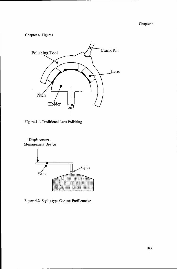
Chapter 4. Figures
I . I . ~
Figure 4.1. Traditional Lens Polishing
Displacement Measurement Device
I Pivot
~tylus
Figure 4.2. Stylus type Contact Profilometer
Chapter 4
CrankPin
Lens
103

~Reference ;------- Flat
Figure 4.3. Fizeau Interferometer
Laser
Lens Under Test
~
Induce4 Shear
Figure 4.4. Lateral Shear Interferometer
Test Surface
Chapter 4
104

Chapter 4
Chapter 4. References
1. Frank Twyman, "Chapter 3, The Nature of Grinding and Polishing", in Prism and
Lens Making, Adam Hilger, London UK, pp 49-66, (1988).
2. Gordon Doughty & James Smith, "Microcomputer-controlled polishing machine
for very smooth and deep aspherical surfaces", Applied Optics, Vol. 26, No. 12, pp
2421-2426, (1986).
3. Sergey Solk, Sergey Shevtsov & Alexi Iakovlev, "Designing of optical elements
manufactured by diamond turning", Advanced Optical Manufacturing and Testing
Technology, Proceedings ofSPIE Vol. 4231, pp 181-188, (2000)
4. Han Rongjiu & Gavin F. Chapman, "Results achieved in the generation of
complex surfaces using deterministic ultra-precision machining systems and
processes", Advanced Optical Manufacturing and Testing Technology, Proceedings
ofSPIE Vol. 4231, pp 175-179, (2000)
5. K. Becker, B. Dorband, R. Locher & M. Schmidt, "Aspheric Optics at Different
Quality Levels and Functional Need", EUROPTO Conference on Otical Fabrication
and Testing, SPIE Vol. 3739, pp 22-33, (1999).
6. Zhang Feihu, Li Wei & Qiu Zhongjun, " Application ofELID grinding technique
to precision machining of optics", Advanced Optical Manufacturing and Testing
Technology, Proceedings ofSPIE Vol. 4231, pp 218-223, (2000)
7. Harvey M. Policove, "Next Generation Optics Manufacturing Technologies",
Advanced Optical Manufacturing and Testing Technology, Proceedings of SPIE
Vol. 4231, pp 8-15, (2000)
105
Chapter 4
8. S. Jacobs, J. Ruckman, E. Fess, D. VanGee, C. Cotton, S. Moore, E. Cleveland &
D. Golini, "Real world examples demonstrate manufacturing of aspheres"
Convergence, pp 1-3, January/February (2000).
9. J. WiIIiam Foreman Jr., "Simple numerical measure of the manufacturabiIity of
aspheric optical surfaces", Applied Optics, Vol. 25, No. 6, pp 826-827, (1986).
10. Feng Zhijing, Wu Hongzhong, Guo Zhengyu, Zhao Yan, "Fabrication of free
form lens with computer-controlled optical surfacing", Advanced Optical
Manufacturing and Testing Technology, Proceedings of SPIE VoI. 4231, pp 194-
201, (2000)
11.Warren J. Smith, "Chapter 14, Optics in Practice", in Modem Optical
Engineering the Design of Optical systems 2nd Edition, pp 463-514, McGraw-HiII
Inc. (1990).
12. Daniel Malacara, "Chapter 17, Contact and Noncontact ProfiIers", in Optical
shop Testing 2nd Edition, John Wiley & Sons Inc, USA, pp 687-714, (1992).
13. David M. G. Stevens, "The application of optical techniques to aspheric surface
measurement", Int. J. Mach. Tools Manufact., VoI. 32., No. Yz, pp 19-25, (1992).
14. Wang Quandou, Zhang Zhongyu, Zhang Xuejun and Yu Jingchi, "Novel
profiIometer with dual digital length gauge for large aspherics measurement",
Advanced Optical Manufacturing and Testing Technology, Proc. SPIE, VoI. 4231,
pp 39-47, (2000).
15. Franke ShiIIke, "Critical aspects on testing aspheres in interferometric setups",
EUROPTO Conference on Optical Fabrication and Testing, Berlin, SPIE VoI. 3739,
pp 317-325, (1999).
106

Chapter 4
16. Daniel Malacara, "Chapter 1 Newton, Fizeau and Hadinger Interferometers", in
Optical Shop Testing 2nd Edition, John Wiley & Sons Inc, USA, pp 1-50, (1992)
17. 1. D. Briers, "Best-fit spheres and conics as an aids in the manufacture and
testing of diamond-turned aspheric optics", Optic a Acta, Vol. 32, No. 2, pp 169-178,
(1985).
18. Ho-Jae Lee, Seung-Woo Kim. "Precision profile measurement of aspheric
surfaces by improved Ronchi test", Optical Engineering, Vol. 38, No. 6, pp 1041-
1047, (1999)
19. K. Creath, V-V. Cheng and J.C. Wyant, "Contouring surfaces usmg two
wavelength phase-shifting interferometry", Optica Acta, Vol. 32, No. 12, pp 1455-
1464, (1985).
20. D, Malacara and A, Cornejo, "Testing of Aspheric Surfaces with Newton
Fringes", Applied Optics, Vol. 9, pp 837, (1970)
21. Mauro Melozzi, Luca Pezzati, Alessandro Mazzoni, "Testing aspheric surfaces
using multiple annular interferograms", Optical Engineering, Vol. 32, No. 5, pp
1073-1079,(1993)
22. Gordon J. Watt, "Aspheric measurement by scanning interferometry", SPIE Vol.
508, Production aspects of single point machined optics, pp 46-53, (1984).
23. Michael Bray, "Stitching Interferometry and Absolute Surface Shape Metrology:
Similarities", Optical Manufacturing and Testing, Proc. OfSPIE, Vol. 4451, pp375-
383, (2001).
24. Masashi Otsubo, Katsuyuki Okada, Jumpei Tsujiuchi, "Measurement of large
plane surface shapes by connecting small-aperture interferograms", Optical
Engineering, Vol. 33, No. 2, pp 608-613, (1994).
107

Chapter 4
25. Daniel Malacara, "Chapter 4 Lateral Shearing Interferometers", in Optical Shop
Testing 2nd Edition, John Wiley & Sons Inc, USA, pp 123-172, (1992)
26. P. Hariharan, "Simple laser interferometry with variable tilt and shear", Applied
Optics, Vol. 14, pp 1056-1057, (1975).
27. P. Hariharan, B. F. Oreb and Zhou Wanzhi, "Measurement of aspheric surfaces
using a microcomputer-controlled digital radial shear interferometer", Optica Acta,
Vol. 31, No. 9, pp 989-999, (1984).
28. Paul E. Murphy, Thomas G. Brown, Duncan T, Moore, "Interference imaging
for aspheric surface testing", Applied Optics, Vol. 39, No. 13, (2000).
29. J. C. Wyant and P. K. O'Neill, Computer Generated Hologram; Null lens test of
aspheric wavefronts", Applied Optics, Vol. 13, No. 12, pp 2762-2765, (1974).
30. Bemd Dorband and Hans J. Tiziani, "Testing aspheric surfaces with computer
generated holograms: analysis of adjustment and shape errors", Applied Optics, Vol.
24, No. 16, pp 2604-2611, (1985).
31. Steven Amold, "CGH null correctors enable testing of aspheric surfaces using
standard interferometers", SPIE oemagazine, pp 40, (August 2002).
32. K.J. Cross and J. W. McBride, "3-D laser metrology for the assessment of
curved surfaces", in laser metrology and machine performance, editors D.M.S.
Blackshaw, A. D. Hope, G.T. Smith, Southampton, UK, (1993).
108

Chapter 4
33. Klaus Ehrmann, Arthur Ho and Klaus Schindhelm, "A 3-D optical profilometer
using a compact disc reading head", Meas. Sci. Technol., Vol. 9, pp 1259-1265,
(1998).
34. Paul Glenn and Gregg Hull-Alien, "Self-referencing, motion-insenstive approach
for absolute aspheric profiling oflarge optics to the nanometer level and beyond",
Optical Manufacturing and Testing IV, Proc. SPIE, Vol. 4451, pp 313-325, (2001).
35. Tung-Hsein Tsai, Kuang-Chao Fan and Jong-I Mou. "A variable-resolution
optical profile measurement system", Meas. Sci. Technol., Vol. 13, pp 190-197,
(2002).
36. Frank Twyman, "Prism and Lens Making", Chapter 11, Testing Optical Work,
Adam Hilger, London UK, pp 364-421, (1988).
109

Chapter 5
CHAPTER 5
SYNTHETIC APERTURE INTERFEROMETRY
110

Chapter 5
Chapter 5. Synthetic Aperture Interferometry
5.1 Introduction
In the previous chapters, methods used in optical design and manufacture have been
reviewed. In Chapter 2 it was noted that the aberration correction properties of
aspheric optics make them very attractive for the optical designer. Although the
benefits of aspheric optics are clear, their manufacturing, and test costs are often
prohibitive, particularly for small batch production and large aperture elements. In
Chapter 4 it was noted that traditional spherical polishing techniques that produce
elements with both accurate spherical form and a high standard of surface finish are
not appropriate to the generation of aspheric form. The generation of accurate
aspheric form can be achieved using single point diamond turning. However, even
the most sophisticated machines cannot achieve the required surface finish with
most optical glasses. The generation of high quality aspherics for use in the visible
spectrum therefore requires a final polishing step and it the quality control during
this step that introduces significant costs.
Clearly, it is important that the polishing process removes enough material to
provide adequate surface finish without causing deviation from the required aspheric
form that has been generated using a different technique such as single point
diamond turning. As discussed in Chapter 4, standard Fizeau or Newton
interferometers are not usually appropriate to aspheric testing since any significant
deviation from a spherical form results in high frequency fringes that cannot be
resolved using standard cameras. For this reason the testing of aspheric optics is
almost exclusively done by scanning single point measurement techniques along one
or more radial tracks usually using a contacting probe. In effect these devices
measure deviation from a reference surface (or line) that is defined by the path of the
traverse and temperature stabilized, precision mechanics are required.
111

Chapter 5
It is clear that the manufacture of aspheric optics would greatly benefit from a
measurement technique that could be implemented on the machine and used to
control the polishing process. This chapter describes a scanning interferometer that
produces two-dimensional fringe patterns in a manner analogous to a Fizeau
interferometer. However, an essential feature of the interferometer is that the optical
field reflected from the surface of interest is not recorded simultaneously but is
recreated from the coherent superposition of signals obtained from a scanning single
point detector. In this way a synthetic aperture is sampled at a rate that can be
adjusted to suit the spatial bandwidth of the interference pattern and no null plates
are required. For the case of ideally rotationally symmetric aspheric optics, this is
particularly advantageous since the surface can be conveniently scanned whilst
rotating the optic on the polishing machine.
In the following sections the synthetic aperture interferometer concept is discussed
in detail. Scanning source and detector configurations are described and data
processing methods are discussed. The method is demonstrated for the measurement
of a small aspheric deviation from a flat. The extension of this method to measure
optics with large surface gradients is considered.
5.2 Background to the Synthetic Aperture Technique
The technique of aperture synthesis has been known and employed for some time, in
an application known as Synthetic Aperture Radar (SAR). In this technique high
resolution images of the ground are constructed by illuminating the target area many
times whilst moving the radar's send and receive antennas, generally combined into
one antenna. Other uses of SAR include the identification of military vehicles from
the air, and terrain following radar. The technique effectively synthesises a large
antenna by knitting together the returns from a smaller array that is moving relative
to the target area. The distance between the antenna and the target is logged, known
as the range and the azimuth, which is perpendicular to the range is also logged.
Repeating this procedure many times, whilst moving the send and receive antennas
112

Chapter 5
between measurements, results in a set of data that can be combined together to form
an image of the area being sampled. This technique has been used to produce 3-D
maps of the earth's surface from space to a resolution of25ml.
5.3 Synthetic Aperture Interferometer Configurations
Initially, let us consider the testing of an axis-symmetric form that is nominally
spherical. Traditionally this type of optic would be tested on a Fizeau interferometer
as shown in Figure 4.3. A practical measurement would require illumination of the
object with a converging wavefront that is nominally concentric with the surface of
interest. The resulting interference pattern, imaged from any surface (real or virtual)
can then be considered as the interference between the reflected wavefront and an
ideal spherical reference wavefront2• The interference observed, for example, in a
nominally concentric circular arc in the meridional plane, is shown schematically in
Figure 5.1. It is clear that, providing the arc is close to the surface, the optical path
difference (OPD) is twice the surface deviation. Using a traditional Fizeau
interferometer it is also clear that both the illuminating wavefront and the resulting
interference pattern are generated simultaneously.
Since coherent detection is implicit in interferometry it is not necessary to measure a
time-stationary wave front simultaneously and because of this, a larger or more
detailed interferogram can be synthesised over the aperture covered by a scanning
detector. In its simplest form a synthetic aperture interferometer suitable for the
measurement of the optic described above would consist of a single (mono-mode)
send/receive fibre as shown in Figure 5.2. This configuration is similar to that
proposed by Bradley and Jeswiet as a means to measure surface texture3• The fibre
delivers the light from a HeNe laser and is scanned along a nominally concentric
circular arc in the meridional plane. The interference between light reflected from
the surface of interest and the fibre termination is detected by a remote
photomultiplier as a function of fibre position. Providing the distance between the
fibre and the surface is small, it is clear from Figure 5.2, that the OPD is once again
113

Chapter 5
equal to twice the surface deviation. In this case the interference pattern is generated
point by point along the circular arc, depicted in Figure 5.2 by a dashed line, but it is
identical to that obtained by the Fizeau interferometer.
Although greatly simplified the fundamental advantages of synthetic aperture
interferometry are apparent in the example above. First, the path of the scanning
fibre can be adapted to suit the optic of interest. The path of the fibre termination can
be thought of as the "test plate" since it defines the reference surface. In this way, to
test an axially symmetric aspheric surface, the spatial bandwidth of the interference
pattern will be minimised if the fibre moves along a path defined to be a small
distance from the ideal form. In addition, any form that is ideally, axially symmetric
will result in an interference pattern that is also symmetric. Practically, this means
that it is only necessary to sample the interference pattern sparsely as the object is
rotated about the axis of (nominal) symmetry.
It is noted, however, that in the basic synthetic aperture configuration of Figure 5.2,
the surface measurement is made relative to the fibre path. As such the measurement
is inherently sensitive to vibration and the accuracy is ultimately determined by the
accuracy of the fibre path.
Figure 5.3 shows a more robust and practical type of synthetic aperture
interferometer. To avoid unwanted reflection from the fibre termination, the
configuration consists of separate source and receive-fibres that are rigidly mounted
together to form a probe that travels along a defined path in the meridional plane.
The two fibres were clamped into grooves cut into a rigid steel tool. This tool,
complete with send and receive fibres attached, is approximated diagrammatically in
Figure 5.3. Light reflected from both the front and rear optical surfaces of the
element under test is collected at the detector fibre where it is passed to a remote
photomultiplier tube. In this case, if the form of either the front or the rear surface is
known the form of the other can be deduced. Since a differential measurement is
114

Chapter 5
made the method is less sensitive to the path taken by the probe and is inherently
tolerant to vibration. We now analyse this set-up in detail.
5.4 Theory
With reference to Figure 5.3, let the origin of the fibre probe be defined as, (xp,yp),
such that the source and receive fibres are separated by a distance, 2d, and located at
positions (xp-d,yp) and (xp+d,yp) respectively. If it is assumed that the intensities of
the reflections from the front and rear surfaces are approximately equal then the
interference signal can be written as,
where A. = the wavelength
OPD = the optical path difference at a given probe position
10 and <\>0 =.: intensity and phase at the origin, respectively (xp=O).
Let us assume that the exact functional form of the probe path is known and it will
be defined as, yp = g(xp) , and that the exact form of one of the surfaces is also
known. In effect, the latter provides the reference surface and without loss of
generality it will be assumed that it corresponds to the rear surface defined by
Yr = g(xr)' From this, and the probe intensity data, the exact functional form of the
front surface given by y f = h(x f ), can be calculated. The first step is to invert
equation 5.1 to find the OPD such that,
5.1
5.2
Where OPDo = the optical path difference at the origin.
115
Chapter 5
Since the absolute phase of the interference pattern is not recorded in our basic
configuration the fact that most aspheric optics are relatively small perturbations to a
large spherical sag, is recognised and made use of. In this case, the phase of
equation 5.1 is usually monotonic and the inverse cosine in equation 5.2 should be
interpreted as a phase unwrapping operator4•
In general the OPD can be written as the difference of the optical path lengths, OPLr
and OPLr, corresponding to reflections from the front and rear surfaces respectively,
OPD = OPLr - OPLr
These paths can be expanded to give,
and,
Where n = the refractive index
The co-ordinates (Xfl,Yfl), (xa,Ya), (Xf3,Yf3) and (xr,Yr) correspond to the ray
intersections at the front and rear surfaces as shown in Figure 5.3. According to
Fermat's principle these coordinates are those that minimise the optical path lengths
defined by equations 5.4 and 5.5. Therefore, the additional equations can be
derived,
116
5.3
5.4
5.5

Chapter 5
aOPL r = aOPL r = aOPL r = aOPL r = 0
8xfl 8xfl 8x r2 8xf3
Although in principle equations, 5,4, 5.5 and 5.6 are sufficient to deduce the required
surface form as a function of probe position, we have been unable to formulate a
general analytic solution to the problem. However, in practice the desired aspheric
form is known and it is relatively straightforward to use this as an initial guess to the
true form and then to use numerical methods to iterate onto a consistent solution.
The method employed at present is a two-stage process and proceeds as follows.
First the initial estimate of the aspheric surface is used to calculate the ray
intersections (Xfl,Yfl), (xn,yn), (Xf3,yo) and (xnYr), and the OPLs from equations 5,4
and 5.5. Figure 5,4. shows the x- coordinates of ray intersections calculated for a
piano-spherical optic with a radius of curvature of 30mm and a centre thickness of
lOmm and a refractive index ofn=1.5. In this case, the probe consisted of source and
receive fibres that were separated by 0.2mm and moved along a straight line defined
by Yp=llmm. The ray intersections were calculated using the Nelder-Mead Simplex
methods. It can be seen that, for this convex surface, the point of reflection from the
front surface increasingly lags behind the probe position as the latter increases.
Conversely the ray intersections corresponding to the path of the ray reflected from
the rear surfaces lead the probe position. The reverse of these observations would be
true if the surface was concave.
Figure 5.5a shows the OPLs corresponding to the front and rear ray paths. It can be
seen that the path corresponding to reflection from the front surface increases as a
function of probe position while that from the rear surface decreases. Figure 5.5b
shows the change in OPD (OPD -OPDo), which in this case, is approximately 5mm
or 8000 fringes at a wavelength of 632.8nm.
117
5.6

Chapter 5
Once the ray intersections have been found, the difference between the ideal OPD
and that measured by the interferometer is calculated. We assume that deviation
from the surface form causes a relatively large change in the OPD and a relatively
small change in the position of the ray intersections. Differentiating equation 5.3
gives the change, ~OPD, as a linear function of changes to the y co-ordinates, ~Yfl,
~Yf2, and ~Yf3, of the ray intersections at the front surface.
5.7
/). [- n{y, - Y /3 X(x, - x /3)2 + {y, - Y /3)2 ]-1/2 1 + ~ /3 + {y /3 _ Y p X(x /3 - X P - d)2 + {y /3 _ Y P )2 ]-1/2
Since equation 5.7 is linear it is relatively straightforward to invert to find the
deviation from ideal form for example using the sparse least squares method of
Paige and Saunders6• The process can then be repeated until the required accuracy is
found. In practice it has been found that it is rarely necessary to perform greater than
one iteration unless the deviation from ideal form is very large. To illustrate this we
consider the 30mm radius spherical form described above with a fourth power
deviation that might be used to correct spherical aberration. In this case the deviation
from form is about O.06mm at the edge of the lens. Figure 5.6 shows the calculated
deviation from form in a single iteration. The maximum error here occurs at the
extreme of the aperture and here it still remains within 1 %. A 1 % error over a range
of O.06mm is not a trivial error, relating as it does to an excursion from form of
around a wavelength. However, in this example as the error is at the extreme edge
of the lens then it is in an area that is likely to be obscured by the fixturing employed
to mount and secure the lens.
118

Chapter 5
5.5 Implementation and Experiment
In order to assess the feasibility of the technique, a fibre probe was constructed and
used to measure optics that were polished on a standard CNC lathe. The general
layout of the system was that of Figure 5.3, employing a HeNe source laser. The
fibre probe was mounted in the turret of the lathe to traverse the test optic in a
closely controlled fashion. During the measurement, the test optic was rotated at a
constant speed and the fibre probe traversed the optic from the centre to the edge of
the aperture. The receive fibre was connected to a photo-multiplier and the output
signal was digitized on a PC equipped with data capture hardware.
Initial measurements were performed on a 25mm diameter optic, manufactured from
BK7 and nominally flat. The optic was squarely mounted in the chuck. The
alignment in the chuck was checked by illuminating the lens surface with a laser
source and then directing the reflected light off a mirror onto a screen located around
three metres form the lens. The lens was then adjusted such that when the chuck
holding the lens was rotated, the laser spot imaged on the screen remained
stationary. The lens was then rotated at 1000rpm (16.66Hz) while the fibre probe
translated at a feed rate of23mmlmin. In all 30,000 data points were recorded during
the test at a sampling rate of 1000Hz. In essence this means that the optic was
sampled along 60 radial 'spokes' and corresponds to a radial distance between
samples of 0.023mm.
Figure 5.7 shows the raw interference data transformed into Cartesian coordinates.
The parallel fringes show that the optic is not a parallel flat but has a small wedge.
For a nominally flat optic it is straightforward to show that each fringe corresponds
to a deviation of approximately IJ2n where n is refractive index and in this case
corresponds to a wedge angle of 64 J.1rads. It would have been useful to have
produced a corroborative interferometric pattern for the same flat produced on a
conventional interferometer. However, as described below the optical element was
aspherised after the test measurements were taken.
119

Chapter 5
Figure 5.8 shows the raw data from the same optical flat after it was modified by
polishing an annular groove approximately 7mm from the optic's centre using
cerium oxide polish powder and a soft polishing tool. The bottom of this groove can
clearly be seen on the fringe pattern as the lighter area between the two closely
spaced sets of fringes that represent the sloping sides of the groove. The fringes
towards the edge of the optic are closer together than those approaching the centre,
which indicates that the groove has steeper sides at the edge of the optic and flattens
out towards the centre. It can be seen that there is a nominally flat area in the centre
of the optic which remained unpolished. The fringes are largely symmetric which
means that the groove running around the optic is symmetric. The slight asymmetry
in the fringes is due to the wedge of the flat (approximately one fringe in this case)
that was observed before polishing.
Finally the fringe data in Figure 5.8 was unwrapped to give the OPD along each
spoke. Since the surface form is not monotonic the bottom of the groove had to be
inferred from a-priori knowledge and was taken to be the point of minimum fringe
frequency approximately 7mm from the centre of the optic. Following the
processing described in the previous section, the surface form of the optic was
calculated and is shown as a greyscale image in Figure 5.9. The groove can clearly
be seen in this image and the smoothness of the data around any circumferential path
indicates that the random errors are of the order of a few nanometres.
5.6 Discussion of Synthetic Aperture Interferometry and Further Improvements
This chapter has introduced the concept of synthetic aperture interferometry as a
means to measure the surface form of aspheric optics. Although more complicated to
analyse than single-fibre systems (combined send and receive), a two-fibre (separate
send and receive) synthetic aperture interferometer is more straightforward to use in
practice. Since the configuration records the interference between light reflected
120

Chapter 5
from the front and rear surfaces it is very robust and sufficiently tolerant to vibration
to be used as an in-process measurement technique on standard machine tools.
The preliminary results clearly show the potential of the method to measure a small
deviation from flat. However, it is worth considering the problems that occur when
applying the method to curves of small radius.
In terms of ray optics, the first point to note is that at each point along the probe path
the fibres must be capable of sourcing and collecting the rays corresponding to front
and rear reflections. For the case of a single send/receive fibre (or closely aligned
pair) this effectively means that the front surface normal must be included within the
cone defined by the numerical aperture (NA) of the fibre. For typical fibres, this
means that the surface normal must remain within a 15 degree cone.
Alternatively, if the fringe patterns resulting from the superposition of the front and
rear reflected fields are considered, it is clear that the entrance pupil (exit pupil) of
the fibres should be less than the fringe spacing at all points along the probe path.
Since the NA of a monomode fibre is inversely proportional to its entrance (or exit)
pupil diameter, this leads to a similar conclusion to that formed from consideration
of ray optics. However, if the front and back surfaces of the optic are nearly
concentric (or parallel), multimode fibres can be used to increase the NA and the
light gathering power of the probe (as discussed below).
Finally, it is worth commenting on the light efficiency of the system. Here
traditional interferometers that use cameras to record the whole interference pattern
simultaneously have a significant advantage over the synthetic aperture
configuration proposed here since the latter collects only a small fraction of the light
emerging from the source. From the analysis above it is tempting to use specialist
drawn fibres with a reduced entrance (exit) pupil and therefore an increased NA to
make the technique applicable to the widest possible range of aspherics. However, it
is straightforward to show that the light efficiency of the system falls as the fourth
121

Chapter 5
power of the pupil diameter and so it is better to increase the system NA
extrinsically. Since the NA need only be large in the radial direction an anamorphic
lens system is most appropriate and this is the subject of further work.
5.7 Conclusions
In this chapter a synthetic aperture interferometric method has been introduced
which has the potential to provide in-process measurement of the surface shape of
aspheric lenses. The method does not require the use of null or test plates and is
inherently tolerant of machine vibration. A mathematical basis that defines the
technique and that describes how surface profile data can be extracted from the
interferograms generated, has been provided. Proof of principle, is provided through
the measurement of a small aspheric deviation polished on the front surface of a
nominally flat form and random errors ofa few nanometers have been observed. The
application of the method to more general aspheric optics, and limitations of the
present apparatus is discussed. Further work to develop and test the synthetic
aperture technique is discussed in chapter 7.
122

Chapter 5
Chapter 5. Figures
Reflected 2h Wave Front
Reference Wave Front --+----~-(
h Ideal ___ ~r
Surface
Figure 5.1. Schematic ofInterference Pattern
\,\
Real Surface
/
123

/" /
/' /"
OPD=2h Probe
-------// ~~=--=====~4-~~
Figure 5.2. Simplest Form of Synthetic Aperture Interferometry
Chapter 5
h
124

y
Chapter 5
------------
Figure 5.3. Practical Synthetic Aperture Interferometer
Unknown Surface YFh(xr
x
Reference Surface Yr=g(xr)
125

Chapter 5
1 2 3 4 5 6 7 8 9 10
Probe Position xp (mm)
Figure 5.4. x-eo-ordinates of Ray Intercept for a PIano-Spherical Optic
126

Chapter 5
18
16 OPLr
14
12
,.-10 e
e '-.....J
8 ~ 0
6 OPLf
4
20 1 2 3 4 5 6 7 8 9 10
Probe Position xp (mm)
Figure 5.5a. Optical Path Length for Front and Rear Paths
127

Chapter 5
0
-0.5
-1
-1.5
..-.. -2 e e '-'
-2.5 Cl ~ 0
-3
-3.5
-4
-4.5
-50 1 2 3 4 5 6 7 8 9 10
Probe Position xp (mm)
Figure 5.5b. Change in Optical Path Difference
128

Chapter 5
0.06
0.05
,.-. 0.04 e e '-'
E 0.03 0 ~
e 0.02 0
tl:: c:: 0 .~
0.01 .;; 11)
Cl
0
-0.010 1 2 3 4 5 6 7 8 9 10
Probe Position xp (mm)
Figure 5.6. Calculated Deviation from Form After One Iteration
Figure 5.7. Interference Data for an Optical Flat
129

Figure 5.8. Interference Data for a Grooved Lens
Surface Height (mm) 0
-0.0017 Figure 5.9. Greyscale Image of Lens Surface.
Chapter 5
130

Chapter 5
References
1. l.P. Fitch, Synthetic Aperture Radar (Springer-Verlag, Berlin, 1987).
2. Max Born, Emil Wolf, "Elements of the Theory of Interference and
Interferometers," in Principles of Optics, (Cambridge University Press, Cambridge,
1997), ,Chap. VII, pp 256-367.
3. C. Bradley, l. leswiet, "An Optical Surface Texture Sensor Suitable for
Integration into a Coordinate Measuring Machine," Annals of the CIRP, Vol.48
No.l, pp.459-462 (1999).
4. D.C. Ghiglia, L.A. Romero,"Robust two-dimensional weighted and unweighted
phase unwrapping that uses fast transforms and iterative methods," Applied Optics
VoUl, No.!, pp 107-117 (1972).
5. Lagarias, l.C., l. A. Reeds, M. H. Wright, and P. E. Wright, "Convergence
Properties of the Nelder-Mead Simplex Method in Low Dimensions," SIAM Journal
ofOptimization,Vol. 9 No.!, pp. 112-147, 1998.
6. Paige, C. C. and M. A. Saunders, "LSQR: An Algorithm for Sparse Linear
Equations
And Sparse Least Squares," ACM Trans. Math. Soft., Vol.8, 1982, pp. 43-71.
131

Chapter 6
CHAPTER 6
COMPUTER-AIDED LENS ASSEMBLY (CALA)
132

Chapter 6
Chapter 6. Computer-Aided Lens Assembly (CA LA)
6.1 Introduction
The alignment of compound lenses was discussed in chapter 3. It can be concluded
that currently, most multi-element camera lenses are manufactured on a "right first
time" basis. For complex, high performance systems it is usually cost effective to
check the form of individual lens elements, but the compound system is usually fully
assembled before it is tested as a whole. Since the positional tolerances of lens
elements are often very small, the cost of mechanical fixturing, especially in high
precision applications, is correspondingly high and can quite easily overwhelm all
the other costs. For this reason, tolerancing must be considered at an early stage in
the optical design process and "right first time" assembly is rarely achieved In
practice for high performance systems.
In many branches of optical engineering, the active alignment of components is now
routine. That is, the system performance is measured in some way during the
alignment and the position of components is varied to optimise this parameter. For
example, single mode optical fibres are manipulated in this way before they are
fused 1• Although some attempts at active alignment have been made [see section
3.3] these methods usually require spacers or other high precision fixturing to be
made. In principle, however, it should be possible to produce flexible fixturing to
hold and manipulate individual elements during alignment, and once aligned the
relative position of the elements can be retained in position by fixing them to a low
precision split casings. This concept is illustrated in Figure 6.1. For the case of
compound lenses the advantage of this approach would be significantly reduced
costs in the production of precision metalwork and less time wasted during the
test/modification cycles.
The work by Rafael Navarro and Esther Moreno-Barrius02 demonstrated that
aberrations in optical systems can be measured by introducing narrow laser beams
133

Chapter 6
into the optical system and recording the position of each at the image plane,
effectively making the system a physical realisation of numerical ray tracing. In the
system described in this chapter, an array of physical rays in the form of Gaussian
laser beams is generated and their path is measured to assess the performance of the
system being aligned. In a similar manner to ray tracing packages used for design
optimisation, a computational or geometric ray trace is then used to find the
positional errors most likely to account for the path of the physical rays, and the
system is improved by making iterative adjustments. We refer to this method as
computer aided lens alignment (CALA) and will now discuss it in detail.
6.2 The CA LA Method
The aim of the CALA method is to actively align the elements in a compound lens
system to achieve performance goals. The alignment process begins by loading the
lens elements into a jig that allows position and orientation of each element, (in
terms of decentration, tilt and axial position) to be adjusted independently.
Adjustments are then made according to the results of a physical ray trace and once
satisfactory performance has been achieved, the elements are cemented into shells to
form compound assemblies or lens groups as required.
With reference to Figure 6.2, it is clear that each element requires five variables to
define its position (x,y,z) and orientation (ex, ey) in three-dimensional space. Let us
define x n ·, as the j'th degree of freedom of the n'th element such that for a ,J
compound lens consisting ofN rotationally symmetric elements, n = 1 to N, j = 1 to
5, such that there are 5N degrees of freedom.
Let the performance of the lens system be measured by the propagation path of M
rays through the system as shown in Figure 6.3. In general, a ray can be completely
defined by the co-ordinates of its intersection in two planes, that is by 4 variables. In
a similar manner to the degrees of freedom, we represent the ray set in suffix
notation by rm,k' where m = 1 to M and k = 1 to 4. Following propagation through
134

Chapter 6
the system we measure the intersection of the return rays in two planes A and B as
shown in Figure 6.3. If Am,i represents the i'th co-ordinate (i = 1 to 2) of the m'th ray
in plane A
6.1
6.2
In general then, given knowledge of the system variables such as the materials and
profiles of the individual optical elements, it is possible to calculate the ray intersects
that correspond to a given ray set and positional variables using computational ray
tracing techniques. The problem, here, is to invert the process to find the positional
variables of the lens elements, given a set of ray intersects. Since f and g are non
linear functions, this is best done using an iterative process. To this end we define an
error function E, such that,
6.3 m=!toM i=!to2 m=!toM i=!to2
where
A'm,i = f(x'n,j' rm,k) 6.4
B'm,i = g(x'n,j' rm,k) 6.5
and Xnj and x' nj are denoted the ideal (design) position variables and an estimate of
the real position variables respectively. The design values would usually be used as
starting estimates of the real position variables and, for the case discussed in the
experiment section, progressive estimates were obtained using the Nelder-Mead
135

Chapter 6
Simplex method of optimisation3• Following iteration, the values of x' nj that
minimise the error are used to calculate the required positional change given by
~n,j = Xn,j - X'n,j 6.6
The process can then be repeated until the positional errors are within the allowed
tolerances. The speed at which the process converges depends on the complexity of
the system the number of rays traced and the precision to which they are measured.
In order for the optimisation routine to identify the positional errors within the
system it is clear that there must be more independent measurements of the system
performance than there are degrees of freedom. If, as above, M ray intercepts are
measured in both A and B planes there are at most, 4M independent measurements
of system performance. It is clear therefore that a rotationally symmetric system
with N elements and SN degrees of freedom requires an integer number of rays to be
traced such that,
M>SN/4 6.7
The central feature of the CALA approach is the physical ray trace that is used to
measure system performance. Although other methods could be employed, such as
interferometric testing4 or Shack-Hartmann wave-front sensing5, the method was
chosen due to its simplicity. There are, however, limitations to the technique. In a
geometrical (or computational) ray trace there is no restriction to the number of rays
that can be traced. However, a physical ray is a pencil beam of finite cross section
that, due to diffraction, must diverge as it propagates. In addition, it is clear that the
power of each surface will also affect the beams divergence and higher order
aberrations will affect the distribution of intensity as the ray passes though the
system.
136

Chapter 6
In this investigation it is assumed that the path taken by the centre of intensity of a
physical ray closely approximates that of a geometric ray. A further assumption was
that to ensure this the physical rays must not overlap each other within the lens
system under test. This second assumption might not be necessary in practice and it
clearly restricts the number of physical rays that can be traced simultaneously.
However, it means that the physical rays sample independent regions of each surface
and for this reason the generation of the physical rays were based on this criterion.
Figure 6.4 shows a single physical ray passing through a unit magnification, imaging
lens system. The ray has been chosen since it crosses the optical axis at the design
conjugates and would therefore be expected to be relatively free of aberration. The
ray is generated such that it has a Gaussian profile with a beam waist at the first (and
second) principle plane of the lens system. With the beam waist in this position it is
straightforward to show that the lens system has no effect on the beam divergence
and the beam radius at the measurement plane, A, is due exclusively to free space
propagation from the second principle plane, PP2. According to the laws governing
the propagation of Gaussian beams6, at a wavelength A, the beam radius, rz, at a
distance Z, from the waist of radius ro, is given by
6.8
If we assume that the beams are readily identifiable providing their spacing is at
least four times their radius in the measurement planes, the minimum beam spacing,
Smin= 4rz and is plotted as a function of beam waist at a wavelength A=SOOnm for a
number of path lengths (Z = 10, 20, SO and 100mm) in figure 6.S. It can be seen that
if the propagation length is of the order of SOmm the minimum separation of the
beams is approximately 0.6 mm. For a typical camera lens with a clear aperture of
lSmm this means that around 600 rays can be traced.
137

Chapter 6
6.3 The Design of the Test Set-up
The mechanical jig used to hold each of the elements is shown in Figure 6.6. Three
screw driven rods hold the element inside two concentric aluminium alloy rings each
of which tilts and translates on ground steel rods in phosphor bronze bushes. The
translations (decentrations) are driven directly from the ends of the ground steel bars
by Mitutoyo 148-201 micrometer heads opposed by springs. These micrometers
have a stated accuracy of ± 5 microns. The tilting mechanisms employ spring
opposed levers, mounted on the ends of the bars, driven by similar micrometers. The
length of the lever arm combined with the accuracy of the micrometers gives a
positional tilt resolution of 0.02°. In the decentration plane the lenses have a range
of movement of ± 3.25mm, in the airspace parameter ± 7.5mm, in the axial
direction, and in tilt a range of ±12.2° that provides adequate movement to correct
even poorly aligned optical systems with ease. Each pair of rings is held on a u
section carrier that is fixed with a clamp to one of the six ground steel rods that run
the length of the jig. A schematic of the rig with three carriers loaded on it can be
seen in Figure 6.7. Individual carriers are fixed to different rods, and each of these
rods is driven independently, by spring opposed Mitutoyo 149-132 micrometer
heads, which provide the axial (airspace) adjustment for each of the lens elements.
These micrometers have a positional accuracy of±10 microns. Each of these rods is
stabilized by a combination of phosphor bronze bushes and linear bearings to ensure
smoothness and accuracy of movement. These bushes and bearings are fixed into
two end plates, see Figure 6.7. The endplates are then clamped to a lathe bed to
ensure that they do not move and are fixed parallel to each other and that there is no
height change between them. This means that the rods, supporting the carriers, are
parallel to the lathe bed ensuring that when the airspace is altered, there is no need to
readjust the decentration ofthe lenses.
138

Chapter 6
6.4 Experimental Method
Physical ray tracing was accomplished using the configuration shown in Figure 6.8.
Since the performance at a single field point is the only critical parameter, in this
case, a fan of rays that diverge from this point to sample the lens aperture, is
propagated through the system. Accordingly, a ImW He-Ne laser is expanded
through a lOOx microscope objective and a 5/lm spatial filter and the resulting
diverging wave-front then passes through a conditioning mask. Physically, the mask
is a computer generated photographic transparency that provides a 7x7 matrix of
(Gaussian) apodized apertures. It is convenient (and also increases the sensitivity) to
use a plane mirror to reflect the rays back through the system. A cube beam-splitter
is used to separate the outward and return rays and the latter are incident on a CCD
array. Figure 6.9 shows a typical image of the rays recorded by the CCD. In this case
the ray intercept points were measured in a single plane defined by the CCD.
Initially, the location of each rayon the CCD array is estimated by finding the local
maximum of each Gaussian beam. An area of interest that surrounds the peak is then
identified and a more accurate estimate of the ray intercept is found by calculating
the centre of intensity (X, Y) given by,
6.9
where Ii and (Xi,Yi) are the intensity and coordinates of the i'th pixel respectively
and the summation is performed over the identified area of interest. Using this
routine it was found that the ray intersects could be found with a repeatability of
approximately 2/lm across the whole area of the array.
Once the physical ray intercept positions are found, an iterative routine involving a
geometrical ray trace is employed to solve the minimise function presented in
equation 6.3, to find the corresponding positional errors in the alignment of each
139

Chapter 6
element. To allow flexibility, both the geometrical ray tracing and optimisation
routine was written in MA TLAB. In this routine, rays are defined in a matrix from a
start point (the pin-hole) and at each intersection with a surface by a position and a
direction. Each curved surface is defined by its curvature and the position of the
centre of curvature in a global co-ordinate system. Flat surfaces are entered as planes
with their positions and orientations also defined with respect to the global co
ordinate system. In addition the two surfaces that make up the individual lens
elements are linked together and move accordingly when the lens is tilted or
decentered. Within the routine each lens element is tilted about the middle point of
its on-axis centre thickness. The lenses are fixed into the carriers such that the mid
point of their centre thick .. less is inline with the tilt axis of the carrier. It is worth
noting that the order in which the various displacements and tilts are implemented is
important. With reference to Figure 6.2 the convention adopted is that displacements
are made before tilt about the x and y-axes respectively.
The geometric ray trace used 49 rays that pass through both the spatial filter (pin
hole) and each of the apertures in the mask. The ray trace includes the beam-splitter
as this also affects the ray paths and introduces significant spherical aberration.
Initially the lens elements were assumed to be located at their ideal locations and the
corresponding ideal ray intercepts were calculated in the plane of the CCD. The
error function defined by equation 6.3 was then calculated and estimates of the
actual positions of each ofthe elements were found by using the fminsearch function
in MA TLAB (Nelder-Mead Simplex method). The elements were then moved by
amounts corresponding to their estimated displacements and the process repeated
until the lens system performance is within the production tolerances.
6.5 Results
The proof of principle evaluations of the CALA method were completed by actively
aligning a displaced air spaced doublet designed as a high power laser objective. The
140

Chapter 6
lens was purchased from Linos Photonics (catalogue number LP 033486), has a
clear aperture of22mm, and an effective focal length of 120mm.
Preliminary investigations concerned the correction of small decentrations of one of
the elements from the ideal configuration. Initially the microscope objective, pin
hole, beamsplitter and mask were removed from the system (Figure 6.8) as were the
lens elements, and the mirror and CCD array were aligned along the optical axis
such that the mirror plane was perpendicular to the optical axis and the laser
(coincident with the optical axis) intercepted the centre of the CCD array. Next the
lenses were loaded into the carriers, the microscope objective was placed in the
system and the tilt, decentration and airspace of the elements were adjusted such that
a single, diffraction limited beam was observed to propagate back through the
system. This was taken to be the ideal configuration for the doublet lens. Once this
was determined the pinhole, mask and beam-splitter were re-introduced to the
system. One of the lenses was then decentered a known amount and the CALA
method was employed to correct for the known assembly flaw.
The first error introduced was a + 1 00 micron decentration in the z-direction of the
rear element. In the first iteration, the optimisation routine attributed the error to a
combination of front element decentration in the negative y-direction and the rear
element in the positive y-direction. In this way, the program attempted to correct for
the decentration by splitting the error between the elements and in effect aligned the
lens along an optical axis that was approximately 60J.lm higher, yet parallel to the
original axis. The corrections were implemented and the performance was
reassessed as before. The program now suggested that lenses were 42J.lm from the
optical axis and the iteration was run once again. When the final image was analysed
the front element was predicted to be 3 microns too low and the rear element was 6
microns too high. This is within the resolution of the micrometer driven mechanical
positioning rig. Using the OSL07 lens design package the residual misalignment was
found to be within the tolerances allowed for diffraction-limited performance. This
experiment was repeated several times with similar outcome.
141
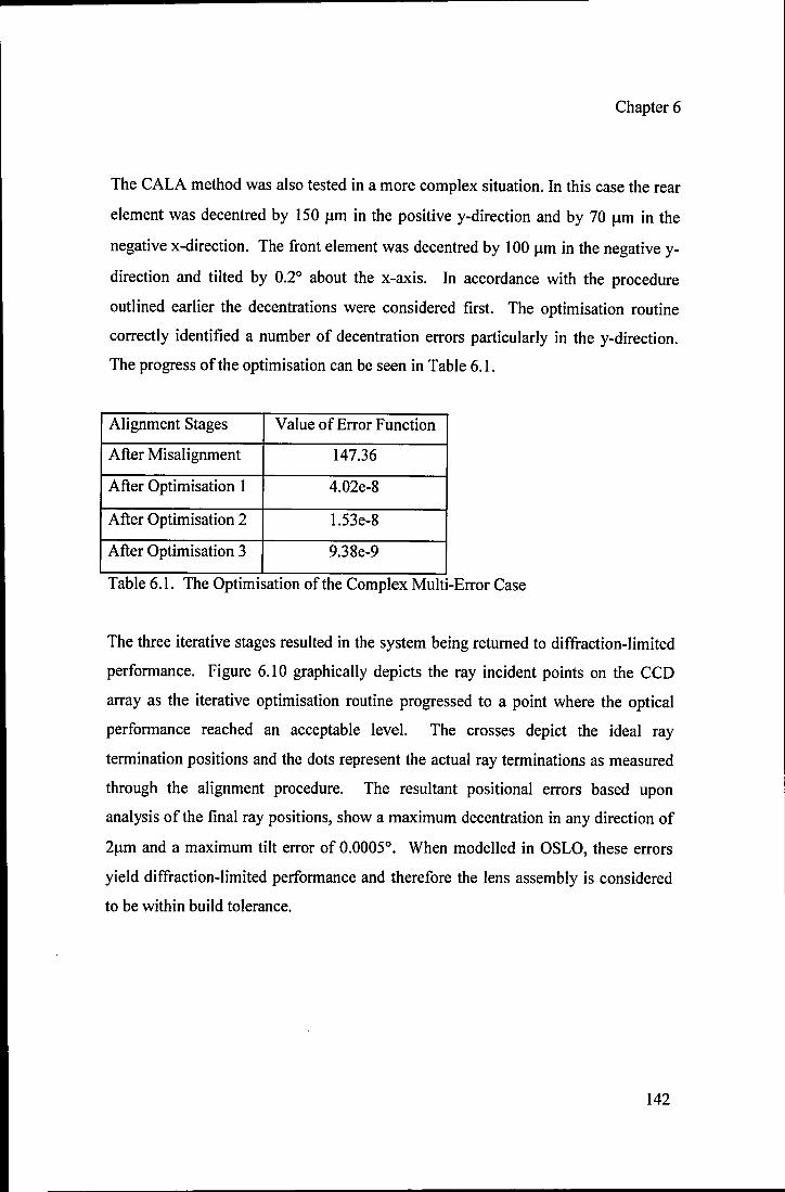
Chapter 6
The CALA method was also tested in a more complex situation. In this case the rear
element was decentred by 150 I!m in the positive y-direction and by 70 I!m in the
negative x-direction. The front element was decentred by 100 flm in the negative y
direction and tilted by 0.2° about the x-axis. In accordance with the procedure
outlined earlier the decentrations were considered first. The optimisation routine
correctly identified a number of decentration errors particularly in the y-direction.
The progress ofthe optimisation can be seen in Table 6.1.
Alignment Stages Value of Error Function
After Misalignment 147.36
After Optimisation 1 4.02e-8
After Optimisation 2 1.53e-8
After Optimisation 3 9.38e-9
Table 6.1. The OptlmlsatlOn of the Complex MultI-Error Case
The three iterative stages resulted in the system being returned to diffraction-limited
performance. Figure 6.10 graphically depicts the ray incident points on the CCD
array as the iterative optimisation routine progressed to a point where the optical
performance reached an acceptable level. The crosses depict the ideal ray
termination positions and the dots represent the actual ray terminations as measured
through the alignment procedure. The resultant positional errors based upon
analysis of the final ray positions, show a maximum decentration in any direction of
2flm and a maximum tilt error of 0.0005°. When modelled in OSLO, these errors
yield diffraction-limited performance and therefore the lens assembly is considered
to be within build tolerance.
142

Chapter 6
6.6 Discussion and Conclusions
A computer aided lens assembly method has been proposed and developed that
allows concurrent test and adjustment of the position of each of the elements until
satisfactory performance is reached. Results have been obtained that show that the
optical system can be aligned to a high degree of accuracy within 3 iterations even
when optimising a number of different positional errors. It is interesting that the
process of physical and geometric ray tracing does not find the correct alignment
immediately but seems to divide the error between the various elements in its initial
assessment. It appears that the error surface is slowly varying and that noise and
other measurement errors cause the optimisation routine to stop in local minima.
When the elements are repositioned, however, small inaccuracies of the mechanical
positioning system appear to introduce sufficient perturbation to move the system
out of these minima and allow it to proceed rapidly along the path to correct
alignment. In this way the iterative alignment method can be viewed as a closed loop
control system and relieves the need for a high accuracy mechanical positioning
system.
Once the optical system has been correctly aligned it is proposed that a split casing
is cemented in place by applying UV curing or two-part epoxy adhesives to the edge
of the lens elements to form a complete compound assembly or lens group. In this
way, it is clear that the casing does not have to be manufactured to exacting
tolerances and is expected to be considerably cheaper to produce than conventional
lock-ring assemblies. However, this phase of the assembly process has not been
tested and further work is required to assess the best adhesives and fixturing for
commercial lens systems.
143
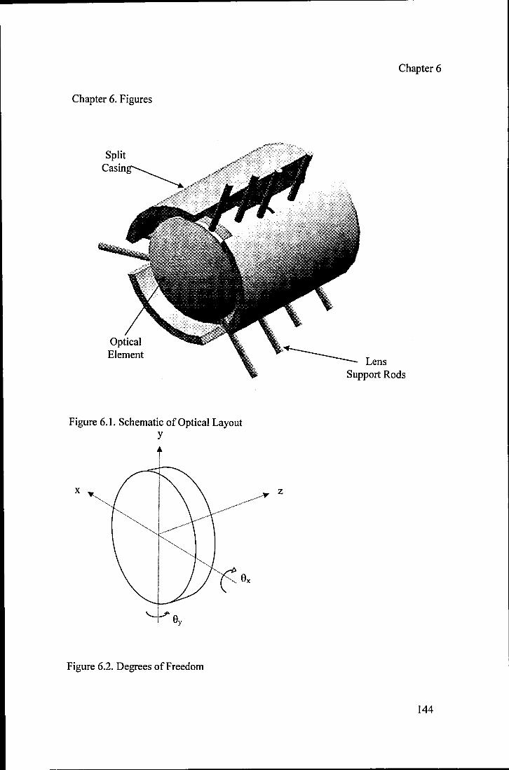
Chapter 6. Figures
Figure 6.1. Schematic of Optical Layout y
t :
x ~ ................ . . ....................................... ...
....... ;:::> ( ......... ex
~e : y
Figure 6.2. Degrees of Freedom
z
Chapter 6
~Lens Support Rods
144

rm,k
Figure 6.3. Geometric Ray Trace
o
Gaussian Profile
~.. : \1
. \ I .. " I
Lens System
PPl PP2
Waist
Figure 6.4. Analysis of Physical Ray Trace
Chapter 6
Am,i
Plane A Plane B
A B I
z
145

Chapter 6
1.4
1.2
/iZ=100mm
Smin 0.8 Z=50mm (mm) Z=20mm
0.6 Z=10mm
0.1 0.2 0.3 0.4 0.5 0.6 0.7 0.8 0.9
ro (mm)
Figure 6.5. Minimum Ray Spacing as a Function of Beam Waist.
Tilt Micrometer
Locking Clamp
Tilt Micrometer
Figure 6.6. Individual Carrier and Lens Assembly
Micrometer Ring Tilts about Horizontal Axis
Decentration Micrometer
Phosphor Bronze Bush
_-tt-t-t--t- Ground ---r-_"l Steel Rods
---4-1-_U-Section Carrier
146

Chapter 6
Figure 6.7. Rig Assembly
CCDArray
Laser Mask
Figure 6.8 Experimental Configuration
147

Chapter 6
Figure 6.9. Typical CCD Image
Target Ray Intercept Points Displaced Ray Intercept Points
2 2 ...;.. + + + + • • • • • • • eL eL L ~ ~- ~ •
1 ••••••• 1 L -- ~- L ~- ~ ... ~ ..
• • • • • • • et- a.. .. e- et- ~ ~ o ••••••• 0 ~ ~ et- e- a.. ~ ~
• • • • • • • ~- ~ et- a.. a.. ~ ~ -1 ••••••• -1 ... ~ ~ er- L ~ ... er···
• • • • • • • • • • • • e e
-2 -2
-2 -1 o 1 2 -2 -1 0 1 2
Ray Intercept Points after First Iteration Corrected Ray Intercept Points
2 2 et- - .- -+- J- -+-• • • t .- .. e- 4! 4!- •• t!-et- et- ....L t et- -+-• .. • 1 1 .- .... .. .. .... .... t!--+- -+- --'-- ~ t t t .. . ' • • e- .. e- .... .... t!- .... -!- .t- -l- t ~- =t. • .' • • o 0 .. .... .. t!- tI- .- 4!-iJ- -f- -I" ..... + .f- t • • • • t!- •• .. tI- tI- e{- 4! t -+- ,
et- et-• • • .. -1 -1 • .... e- e- tI- 4!- .... _L -!- -+- it .--:- -+-• • • • .' .. .... t!- e- .- * t!-
-2 -2
-2 -1 o 1 2 -2 -1 0 1 2
Figure 6.10. The Iterative Correction of the Multiple Error Example
148
Chapter 6
References
1. D.T. Pham, M. Castellani, "Intelligent control of fibre optic components
assembly", Proc. Instn. Mech. Engrs, Vol. 215, Part B9, pp 1177-1189, (2001)
2. Rafael Navarro, and Esther Moreno-Barriuso, "Laser ray-tracing method for
optical testing", Optics Letters, Vol.24, No. 1, pp 951-953, (1999).
3. Lagarias, J.C., J. A. Reeds, M. H. Wright, and P. E. Wright, "Convergence
Properties of the Nelder-Mead Simplex Method in Low Dimensions," SIAM Journal
ofOptimization,Vol. 9 No.1, pp. 112-147, (1998).
4. Alberto Jaramillo-Nunez, David M. Gale, Alejandro Cornejo-Rodriguez,
"Apparatus for cementing doublet lenses", Opt. Eng., Vol. 35, No. 12, pp 3432-
3436, (1996).
5. L. Seifert, J. Liesener, H.J. Tiziani, "The adaptive Shack-Hartmann sensor",
Optics Communications, Vol. 216, No. 4-6, pp 313-319, (2003).
6. Frank L. Pedrotti, Leno S. Pedrotti, "Characteristics of Laser Beams", in
Introduction to Optics 2nd Edition, (Prentice-Hall International Inc, Upper Saddle
River, New Jersey, 1996), pp 456-483.
7. OSLO Premium Edition Revision 6.1, Lambda Research Corporation, Littleton,
Massachusetts, USA, 2001.
149

CHAPTER 7
CONCLUSIONS AND FURTHER WORK
Chapter 7
150

Chapter 7
Chapter 7. Conclusions and Further Work
7.1 Summary
This thesis has described all aspects of the optical system production process, from
the development of a specification through to the assembly of the finished article.
Each stage has been discussed in detail with reference to traditional and modem
practices and how these can be further improved upon. Throughout the work there
has been an aim to reach a closer control of each stage of production.
At the design stage there is the desire to include the tolerances and associated cost
within the optimisation stage in order to make them concurrent rather than
consecutive, resulting in design towards an economic as well as high optical
performance. A description of the manufacture of individual optical elements has
been presented combined with how these elements are quality tested. Again the
benefits of combining these two stages, such that surface form measurements can be
taken while the lens is being manufactured and then any errors in the surface form
can be corrected, have been highlighted. The desirability of aspheric surfaces has
been detailed along with the challenges that these surfaces pose in terms of
manufacture and especially test. A new type of interferometer has been developed
that is applicable to on-machine and in-process optical testing without the
requirement for separate purpose made reference surfaces of any kind.
The problem of optical assembly was then addressed. The current method employed
for assembling multi-element optical systems involves building the complete system
or at least significant sub-assemblies before testing its performance. If the system
does not reach the required levels of performance then it must be disassembled and
rebuilt until the performance criteria is reached. Progress has been made, during the
course of this research, towards the development of a closed loop system to aid the
alignment of optical systems at the assembly stage, which allows the alignment and
151

Chapter 7
positioning of each of the elements within the system before they are fixed within
the mechanical components that provide the body of the unit.
7.2 Conclusions
It can be concluded from the discussions on lens design that the optimisation of
optical systems is presently carried out solely on the optical performance of the
system. The application of tolerance analysis and costing are only carried out once
the optical design has been completed. If the system is too costly or difficult to
manufacture then it must be re-designed, and there are obvious expense and time
implications in doing this. The use of aspheric surfaces within optical designs can
yield a multitude of benefits in such areas as aberration control and reduction of
system complexity though at present the use of aspheric lenses is considered too
expensive for the majority of applications.
The investigations into optical tolerancing have provided an insight into the
multitude of parameters that have to be considered. Attention has been drawn to the
fact that the tolerances can have a large impact on the assembly as well as the
manufacturing tolerance. Badly judged tolerances could have an inordinately large
effect on the cost of an optical system especially if they cause a sharp rise in the
rejection rate. In order to generate a comprehensive cost function, the base line
information must be very specific to the manufacturing and assembly techniques that
a given company employs and it would be best practice to develop this base line data
from production data at the company. The design example presented showed that it
is possible to include some cost parameters within the optimisation routines but only
for simple and specific cases. A general error function that would take into account
an accurate measure of lens cost as well as performance would have to be extremely
complex and, as optimisation times rise approximately with the square of the
number of variables involved, would require an unfeasible amount of both
computing power and run time. After this rudimentary investigation, it was decided
that in the near future the cost of lenses is more likely to decrease through
152

Chapter 7
improvement of the manufacture and assembly processes. In terms oflens polishing
it is clear that traditional grinding and polishing techniques are unable to generate
the deeply aspheric surfaces that are becoming more common in lens designs. New
surface generation techniques have been developed including single point diamond
turning and MRF, which do not require the rigid tools oftraditional methods and are
more able to produce aspheric surfaces. These new techniques would benefit greatly
from an on-machine surface measurement system that would enable an iterative
process of test and correction until the desired surface form is reached. A
specification of an ideal test system was drawn up listing such criteria as in-process
measurement and flexibility without the need for costly reference surfaces (either
real or computer generated).
A new type of interferometer has been developed and it has been termed Synthetic
Aperture Interferometryl as it shares some principles with the established technique
of Synthetic Aperture Radar. This technique is capable of producing full aperture
interference patterns analogous to those produced by a Fizeau interferometer. The
method is capable of measuring surface form of even aspheric lenses without the
requirement for separate reference surfaces. The system is inherently resistant to
vibration and is simple and robust making it eminently suitable for on machine
applications.
From the literature, together with two years experience working in a lens assembly
environment, it was concluded that there is also scope to improve the optical
assembly process. A new assembly rig and method has been developed that employs
computer-aided alignment, CALA 2, of the optical system during the alignment
system. This method ensures that when the elements are fixed into their respective
mechanical housing they are aligned to within the tolerance required and the lens
performs up to the designer's expectations.
153
Chapter 7
7.3 Further Work
There are two main areas of thesis where there is scope for further work. The
Synthetic Aperture Interferometry technique requires development until it is ready
for integration into the production environment. Further investigation and
subsequent trials are needed in the final stage of the CALA process where the lenses
are cemented to their metal work.
In terms of the lens surface measurement, an area that needs to be looked at is
increasing the variety of curvatures that can be assessed. There is a need to
demonstrate the method on a highly curved surface. Testing such a surface would
require the numerical aperture of the fibre probe to be increased. Noting that the NA
need be increased in the radial direction only, this can be achieved by introducing an
anamorphic, lens into the system in front of the fibre probes. A schematic of the
optical layout of a wide-angle of acceptance probe can be seen in Figure 7.1. This
should increase the acceptance angle of the fibres such that steep curves can be
examined. The design ofthe tool needs to be re-examined and adapted such that it is
suitable for integration into the current CNC optical processing machines. A process
would have to be introduced to clean the lens on the machine before the
measurement is taken, and a method of ensuring the measurement probe is kept
clean in the polishing environment. This will ease the introduction of the technique
into the production environment. The control software needed to integrate with the
polishing machines must be developed and also a front end user interface for the
software to enable others to use the system. There is also scope to improve the
method by which the results are processed. At the current stage of development an
iterative search method is used to determine the shape of the test surface. It may be
better to strive for a closed form solution to the problem of inverting the path length
and surface form equations, or to employ a finite-difference type approach.· Further
investigation is also required into the deviation from surface form error highlighted
at the end of Section 5.4. The iterative search method of determining deviation from
form needs to be repeated to determine whether the 1 % error at the extreme of the
154

Chapter 7
aperture can be reduced by employing more iterations. In addition, the method
requires testing for a variety of aspheric and spherical surfaces to gain a greater level
of confidence in its accuracy and if necessary refine the method.
The final stage of the CALA method also requires further investigation. Some
improvements could be made to the mechanical design of the rig such as including a
method by which the individual elements can be rotated about their optical axes such
that the system take account of lenses that are non-rotationally symmetric.
However, this would require significant changes to the optimisation software to take
into account non-rotationally symmetric items and may have to include some form
of trial and error optimisation routine. The structure of the rig needs to be altered to
create a more solid base for the technique. This could be achieved by grouping the
bushes in each yoke in a much more tightly packed arrangement thus lowering the
likelihood of a twisting moment on the yoke which in turn causes uneven motion.
The springs, which oppose the movement in the system, need to be stronger which
will act to improve the independence of each axis of motion. The types of cement
used to fix the lenses to the lens body need to be researched possibly using two-part
UV curing epoxy cements, which are already widely used in the optical production
environment. The cement must be carefully chosen. It must be viscous enough to
stay in the casing as it is manipulated into position. At present it is envisaged that
the metal work cemented around the lenses effectively be a split version of the
stepped-cylindrical barrels currently used to house optical elements. The barrel
would be turned as a single cylindrical unit and then split using a saw or milling
machine. A method for securing the casing in place while the glue cures without
disturbing the position of the lenses must be developed. This topic requires further
research to see whether this technique is the most cost-effective and the accuracies
to which the metal work needs to be machined. The ultimate aim is to automate the
alignment procedure to a stage where the lens progresses from a misaligned to an
aligned system with no operator input. This would require replacing the manual
micrometers with a system that can be computer driven. This could incorporate
servos, inchworm drives or electric motors to provide the motion needed to align the
155

Chapter 7
lenses. An end condition would also have to be incorporated within the software to
ensure that the system does not continue with infinitesimally small adjustments
yielding tiny performance increases.
With the implementation of these techniques it should be possible to decrease the
production costs of compound lens systems, or conversely produce higher
specification systems at a similar cost to the original system.
156

Chapter 7
Chapter 7. Figures
Side View
Top View
I SendlReceive \
Fibre Piano-spherical Lens
Figure 7.1. Schematic ofa High Numerical Aperture Measurement Probe.
157

Chapter 7
References
1. Richard Tomlinson, leremy M. Coupland, 10n Petzing "Synthetic Aperture
Interferometry: In-process measurement of aspheric optics", Applied Optics, Vo!.
42, Issue 4, pp 701-707, (February 2003)
2. Richard Tomlinson, Rob Alcock, 10n Petzing, leremy Coupland, "Computer
Aided Lens Assembly", Applied Optics, Vo!. 43 Issue 3 Page 579 (January 2004)
158