Lectures on Discrete and Polyhedral Geometry

Igor Pak

April 20, 2010

Contents

Introduction 3Acknowledgments 7Basic definitions and notations 8

Part I. Basic discrete geometry

1. The Helly theorem 112. Caratheodory and Barany theorems 203. The Borsuk conjecture 264. Fair division 325. Inscribed and circumscribed polygons 396. Dyson and Kakutani theorems 547. Geometric inequalities 618. Combinatorics of convex polytopes 729. Center of mass, billiards and the variational principle 8310. Geodesics and quasi-geodesics 9611. The Steinitz theorem and its extensions 10212. Universality of point and line configurations 10913. Universality of linkages 11814. Triangulations 12515. Hilbert’s third problem 13916. Polytope algebra 14817. Dissections and valuations 15918. Monge problem for polytopes 17019. Regular polytopes 17720. Kissing numbers 185

1

2

Part II. Discrete geometry of curves and surfaces

21. The four vertex theorem 19322. Relative geometry of convex polygons 20723. Global invariants of curves 21624. Geometry of space curves 22925. Geometry of convex polyhedra: basic results 24126. Cauchy theorem: the statement, the proof and the story 24927. Cauchy theorem: extensions and generalizations 25728. Mean curvature and Pogorelov’s lemma 26329. Sen’kin-Zalgaller’s proof of the Cauchy theorem 27330. Flexible polyhedra 27931. The algebraic approach 28632. Static rigidity 29233. Infinitesimal rigidity 30234. Proof of the bellows conjecture 30735. The Alexandrov curvature theorem 31536. The Minkowski theorem 32237. The Alexandrov existence theorem 32938. Bendable surfaces 33639. Volume change under bending 34040. Foldings and unfoldings 348

Part III. Details, details...41. Appendix 360

41.1. The area of spherical polygons 36041.2. The law of cosines for spherical triangles 36041.3. The irrationality of (arccos 1

3)/π 361

41.4. The Minkowski inequality 36141.5. The equality part in the Brunn–Minkowski inequality 36241.6. The Cayley–Menger determinant 36441.7. The theory of places 36541.8. The mapping lemma 368

42. Additional problems and exercises 37042.1. Problems on polygons and polyhedra 37042.2. Volume, area and length problems 37242.3. Miscellaneous problems 375

Hints, solutions and references to selected exercises 377References 410Notation for the references 432Index 433

3

Introduction

The subject of Discrete Geometry and Convex Polytopes has received much attentionin recent decades, with an explosion of the work in the field. This book is an intro-duction, covering some familiar and popular topics as well as some old, forgotten,sometimes obscure, and at times very recent and exciting results. It is somewhatbiased by my personal likes and dislikes, and by no means is a comprehensive ortraditional introduction to the field, as we further explain below.

This book began as informal lecture notes of the course I taught at MIT in theSpring of 2005 and again in the Fall of 2006. The richness of the material as well asits relative inaccessibility from other sources led to making a substantial expansion.Also, the presentation is now largely self-contained, at least as much as we couldpossibly make it so. Let me emphasize that this is neither a research monograph nora comprehensive survey of results in the field. The exposition is at times completelyelementary and at times somewhat informal. Some additional material is included inthe appendix and spread out in a number of exercises.

The book is divided into two parts. The first part covers a number of basic resultsin discrete geometry and with few exceptions the results are easily available else-where (to a committed reader). The sections in the first part are only loosely relatedto each other. In fact, many of these sections are subjects of separate monographs,from which we at times borrow the proof ideas (see reference subsections for the ac-knowledgements). However, in virtually all cases the exposition has been significantlyaltered to unify and simplify the presentation. In and by itself the first part can serveas a material for the first course in discrete geometry, with fairly large breadth andrelatively little depth (see more on this below).

The second part is more coherent and can be roughly described as the discrete dif-ferential geometry of curves and surfaces. This material is much less readily available,often completely absent in research monographs, and, on more than one occasion, inthe English language literature. We start with discrete curves and then proceed todiscuss several versions of the Cauchy rigidity theorem, the solution of the bellowsconjecture and Alexandrov’s various theorems on polyhedral surfaces.

Although we do not aim to be comprehensive, the second part is meant to be asan introduction to polyhedral geometry, and can serve as a material for a topics classon the subject. Although the results in the first part are sporadically used in thesecond part, most results are largely independent. However, the second part requiresa certain level of maturity and should work well as the second semester continuationof the first part.

We include a large number of exercises which serve the dual role of possible homeassignment and additional material on the subject. For most exercises, we eitherinclude a hint or a complete solution, or the references. The appendix is a smallcollection of standard technical results, which are largely available elsewhere andincluded here to make the book self-contained. Let us single out a new combinatorialproof of the uniqueness part in the Brunn–Minkowski inequality and an elementaryintroduction to the theory of places aimed towards the proof of the bellows conjecture.

4

Organization of the book. The book is organized in a fairly straightforward man-ner, with two parts, 40 sections, and the increasing level of material between sectionsand within each section. Many sections, especially in the first part of the book, can beskipped or their order interchanged. The exercises, historical remarks and pointers tothe literature are added at the end of each section. Theorems, propositions, lemmas,etc. have a global numbering within each section, while the exercises are numberedseparately. Our aversion to formula numbering is also worth noting. Fortunately, dueto the nature of the subject we have very few formulas worthy of labeling and thoseare labeled with AMS-TeX symbols.

The choice of material. Upon inspecting the table of contents the reader wouldlikely assume that the book is organized around “a few of my favorite things” andhas no underlying theme. In fact, the book is organized around “our favorite tools”,and there are very few of them. These tools are heavily used in the second part, butsince their underlying idea is so fundamental, the first part explores them on a moreelementary level in an attempt to prepare the reader. Below is our short list, in theorder of appearance in the book.

1. Topological existence arguments. These basic non-explicit arguments are at theheart of the Alexandrov and Minkowski theorems in Sections 35–37. Sections 4–6and Subsection 3.5 use (often in a delicate way) the intermediate value theorem, andare aimed to be an introduction to the method.2. Morse theory type arguments. This is the main tool in Section 8 and in the proofof the Fary–Milnor theorem (Section 24). We also use it in Subsection 1.3.3. Variational principle arguments. This is our most important tool all around, givingalternative proofs of the Alexandrov, Minkowski and Steinitz theorems (Sections 11,35, and 36). We introduce and explore it in Subsection 2.2, Sections 9 and 10.4. Moduli space, the approach from the point of view of algebraic geometry. Theidea of realization spaces of discrete configurations is the key to understand Gluck’srigidity theorem leading to Sabitov’s proof of the bellows conjecture (Sections 31and 34). Two universality type results in Sections 12 and 13 give a basic introduction(as well as a counterpart to the Steinitz theorem).5. Geometric and algebraic valuations. This is a modern and perhaps more technicalalgebraic approach in the study of polyhedra. We give an introduction in Sections 16and 17, and use it heavily in the proof of the bellows conjecture (Section 34 andSubsection 41.7).6. Local move connectivity arguments. This basic principle is used frequently incombinatorics and topology to prove global results via local transformations. We in-troduce it in Section 14 and apply it to scissor congruence in Section 17 and geometryof curves in Section 23.7. Spherical geometry. This is a classical and somewhat underrated tool, despite itswide applicability. We introduce it in Section 20 and use it throughout the secondpart (Sections 24 and 25, Subsections 27.1, 29.3).

Note that some of these are broader and more involved than others. On the otherhand, some closely related material is completely omitted (e.g., we never study the

5

hyperbolic geometry). To quote one modern day warrior, “If you try to please every-body, somebody’s not going to like it” [Rum].

Section implications. While most sections are independent, the following list ofimplications shows which sections are not: 1⇒ 2, 3, 20 5⇒ 23 7⇒ 28, 369⇒ 10⇒ 25, 40 11⇒ 34 12⇒ 13 14⇒ 17 15⇒ 16⇒ 17 21⇒ 2322⇒ 26⇒ 27⇒ 37 26⇒ 28, 29, 30 25⇒ 35⇒ 37⇒ 38 31⇒ 32⇒ 33

Suggested course content. Although our intention is to have a readable (andteachable) textbook, the book is clearly too big for a single course. On a positiveside, the volume of book allows one to pick and choose which material to present.Below we present several coherent course suggestions, in order of increasing difficulty.

(1) Introduction to Discrete Geometry (basic undergraduate course).§§ 1, 2.1-2, 3, 4, 5.1-2 (+ Prop. 5.9, 5.11), 23.6, 25.1, 19, 20, 8.1-2, 8.4, 9, 10, 12, 13,14.1-3, 15, 21.1-3, 23.1-2, 23.6, 22.1-5, 26.1-4, 30.2, 30.4, 39, 40.3-4.

(2) Modern Discrete Geometry (emphasis on geometric rather than combinatorialaspects; advanced undergraduate or first year graduate course).§§ 4–6, 9, 10, 12–15, 17.5-6, 18, 20–23, 25, 26, 29, 30, 33, 35.5, 36.3-4, 39, 40.

(3) Geometric Combinatorics (emphasis on combinatorial rather than geometric as-pects; advanced undergraduate or first year graduate course).§§ 25.1, 19, 20, 1–4, 8, 11, 12, 14–17, 23, 22.1-5, 26.1-4, 32, 33, 40.3, 40.4.

(4) Discrete Differential Geometry (graduate topics course)§§ 9–11, 21, 22, 24–28, 30–35, 7, 36–38, 40.

(5) Polytopes and Algebra (intuitive graduate topics course)Scissor congruence: §§ 15, 16, 14.4, 17, then use [Bolt, Dup, Sah] for further results.Realization spaces and the bellows conjecture: §§ 11–13, 31, 34, then use [Ric].Integer points enumeration: use [Barv, §7], [Grub, §19] and [MilS, §12].

On references and the index. Our reference style is a bit idiosyncratic, but,hopefully, is self-explanatory.1 Despite an apparently large number of references, wemade an effort to minimize their number. Given the scope of the field, to avoid anexplosion of the references, we often omit important monographs and papers in favorof more recent surveys which contain pointers to these and many other references.Only those sources explicitly mentioned in the remarks and exercises are included. Onoccasion, we added references to classical texts, but only if we found the expositionin them to be useful in preparing this book. Finally, we gave a certain preferenceto the important foreign language works that are undeservingly overlooked in themodern English language literature, and to the sources that are freely available onthe web, including several US patents. We made a special effort to include the arXiv

numbers and the shortened clickable web links when available. We sincerely apologizeto authors whose important works were unmentioned in favor of recent and moreaccessible sources.

1See also page 432 for the symbol notations in the references.

6

We use only one index, for both people and terminology. The references havepointers to pages where we use them, so the people in the index are listed only if theyare mentioned separately.

On exercises. The exercises are placed at the end of every section. While mostexercises are related to the material in the section, the connection is sometimes notobvious and involves the proof ideas. Although some exercises are relatively easy andare meant to be used as home assignments, most others contain results of independentinterest. More often than not, we tried to simplify the problems, break them intopieces, or present only their special cases, so that they can potentially be solved bya committed reader. Our intention was to supplement the section material with anumber of examples and applications, as well as mention some additional importantresults.

The exercises range from elementary to very hard. We use the following ranking:exercises labeled [1-], [1] and [1+] are relatively simple and aimed at students, whilethose labeled [2-], [2] and [2+] are the level of a research paper with the increasinginvolvement of technical tools and results from other fields. We should emphasizethat these rankings are approximate at best, e.g., some of those labeled [1+] mightprove to be excessively difficult, less accessible than some of those labeled [2-]. If anexercise has a much easier proof than the ranking suggests, please let me know and Iwould be happy to downgrade it.

We mark with ♦ the exercises that are either used in the section or are mentionedelsewhere as being important to understanding the material. Some additional, largelyassorted and ad hoc exercises are collected in Section 42. These are chosen not fortheir depth, but rather because we find them appealing enough to be of interest tothe reader.

Hints, brief solutions and pointers to the literature are given at the end of the book.While some solutions are as good as proofs in the main part, most are incompleteand meant to give only the first idea of what to do or where to go. Open problemsand a few simple looking questions I could not answer are marked with [∗]. They arelikely to vary widely in difficulty.

On figures. There are over 250 color figures in the book, and they are often integralto the proofs.

7

Acknowledgements. Over the years I benefitted enormously from conversationswith a number of people. I would like to thank Arseny Akopyan, Boris Aronov, ImreBarany, Sasha Barvinok, Bob Connelly, Jesus De Loera, Elizabeth Denne, NikolaiDolbilin, Maksym Fedorchuk, Alexey Glazyrin, David Jerison, Gil Kalai, Greg Ku-perberg, Gilad Lerman, Ezra Miller, Oleg Musin, Janos Pach, Rom Pinchasi, YuriRabinovich, Jean-Marc Schlenker, Richard Stanley, Alexey Tarasov, Csaba Toth, UliWagner and Victor Zalgaller for their helpful comments on geometry and other mat-ters.

Parts of these lectures were read by a number of people. I would like to thankAndrew Berget, Steve Butler, Jason Cantarella, Erhard Heil, Ivan Izmestiev, Kristof-fer Josefsson, Michael Kapovich, Igor Klep, Carly Klivans, Idjad Sabitov, RamanSanyal, Egon Schulte, Sergei Tabachnikov, Hugh Thomas, Gudlaugur Thorbergsson,Rade Zivaljevic and anonymous reviewers for their corrections and suggestions on thetext, both big and small. Jason Cantarella and Andreas Gammel graciously allowedus to use Figures 42.14 and 39.5. Special thanks to Ilya Tyomkin for his great helpwith the theory of places. Andrew Odlyzko’s suggestion to use the tinyurl linkshelped make the references web accessible. I am also deeply grateful to all studentsin the courses that I taught based on this material, at MIT, UMN, and UCLA, fortheir interest in the subject on and off the lectures.

Finally, I would like to thank my parents Mark and Sofia for their help and patienceduring our Moscow summers and Spring 2008 when much of the book was written.

Igor Pak

Department of Mathematics, UCLA

Los Angeles, CA 90095, USA

pak@math.ucla.edu

8

Basic definitions and notations. Let P ⊂ Rd be a convex polytope, or a generalconvex body. We use S = ∂P for the surface of P . To simplify the notation we willalways use area(S), for the surface area of P . Formally, we use area(·) to denote the(d − 1)-dimensional volume: area(S) = vold−1(S). We say that a hyperplane H issupporting P at x ∈ S if P lies on one side of H , and x ∈ H .

For a set X ⊂ Rd we use cm(X) to denote the center of mass2 and conv(X) todenote the convex hull of X. We use |xy| to denote the distance between pointsx, y ∈ Rd. Alternatively, ‖e‖ denotes the length of a vector e = −→xy. The vectors arealways in bold, e.g., O usually denotes the origin, while 0 is the zero vector. We let〈u ,w〉 denote the scalar product of two vectors. The geodesic distance between twosurface points x, y ∈ S is denoted by |xy|S. We use ∢ to denote the spherical angles.

All our graphs will have vertices and edges. The edges are sometimes oriented,but only when we explicitly say so. In the beginning of Section 21, following a longstanding tradition, we study “vertices” smooth curves, but to avoid confusion wenever mention them in later sections.

In line with tradition, we use the word polygon to mean two different things: botha simple closed piecewise linear closed curve and the interior of this curve. Thisunfortunate lack of distinction disappears in higher dimension, when we consider spacepolygons. When we do need to make a distinction, we use closed piecewise linear curveand polygonal region, both notions being somewhat unfortunate. A simple polygon isalways a polygon with no self-intersections. We use Q = [v1 . . . vn] to denote a closedpolygon with vertices vi in this (cyclic) order. We also use (abc) to denote a triangle,and, more generally, (v0v1 . . . vd) to denote a (d+1)-dimensional simplex. Finally, weuse (u, v) for an open interval (straight line segment) or an edge between two vertices,[xy] and [x, y] for a closed interval, either on a line or on a curve, and (xy) for a linethrough two points.

In most cases, we use polytope to mean a convex hull of a finite number of points.Thus the word “polytope” is usually accompanied with an adjective convex, except inSections 15–17, where a polytope is a finite union of convex polytopes. In addition,we assume that it is fully dimensional, i.e., does not lie in an affine hyperplane. Inall other cases we use the word polyhedron for convex and non-convex surfaces, non-compact intersections of half-spaces, etc. Since we are only concerned with discreteresults, we do not specify whether polytopes are open or closed sets in Rd, and usewhatever is appropriate in each case.

We make a distinction between subdivisions and decompositions of a polytope,where the former is required to be a CW complex, while the latter is not. Thenotions of triangulation is so ambiguous in the literature, we use it only for simplicialsubdivisions. We call dissections the simplicial decompositions, and full triangulationsthe triangulations with a given set of vertices (usually the vertices of a given convexpolytope).

Occasionally we use the standard notation for comparing functions: O(·), o(·),Ω(·) and θ(·). We use various arrow-type symbols, like ∼, ≃, ↔, ⊲⊳, ≍, ⇔, etc.,

2We consider cm(X) only for convex of piecewise linear sets X , so it is always well defined.

9

for different kind of flips, local moves, and equivalence relations. We reserve ≈ fornumerical estimates.

Finally, throughout the book we employ [n] = 1, 2, . . . , n, N = 1, 2, . . ., Z+ =0, 1, 2, . . ., R+ = x > 0, and Q+ = x > 0, x ∈ Q. The d-dimensional Euclideanspace is always Rd, a d-dimensional sphere is Sd, and a hemisphere is Sd+, where d ≥ 1.To simplify the notation, we use X − a and X + b to denote X r a and X ∪ b,respectively.

10

Part I

Basic Discrete Geometry

11

1. The Helly theorem

We begin our investigation of discrete geometry with the Helly theorem and itsgeneralizations. That will occupy much of this and the next section. Although theseresults are relatively elementary, they lie in the heart of discrete geometry and aresurprisingly useful (see Sections 3 and 24).

1.1. Main result in slow motion. We begin with the classical Helly Theorem inthe plane.

Theorem 1.1 (Helly). Let X1, . . . , Xn ⊂ R2 be convex sets such that Xi∩Xj∩Xk 6= ∅for every 1 ≤ i < j < k ≤ n, where n ≥ 3. Then there exists a point z ∈ X1, . . . , Xn.

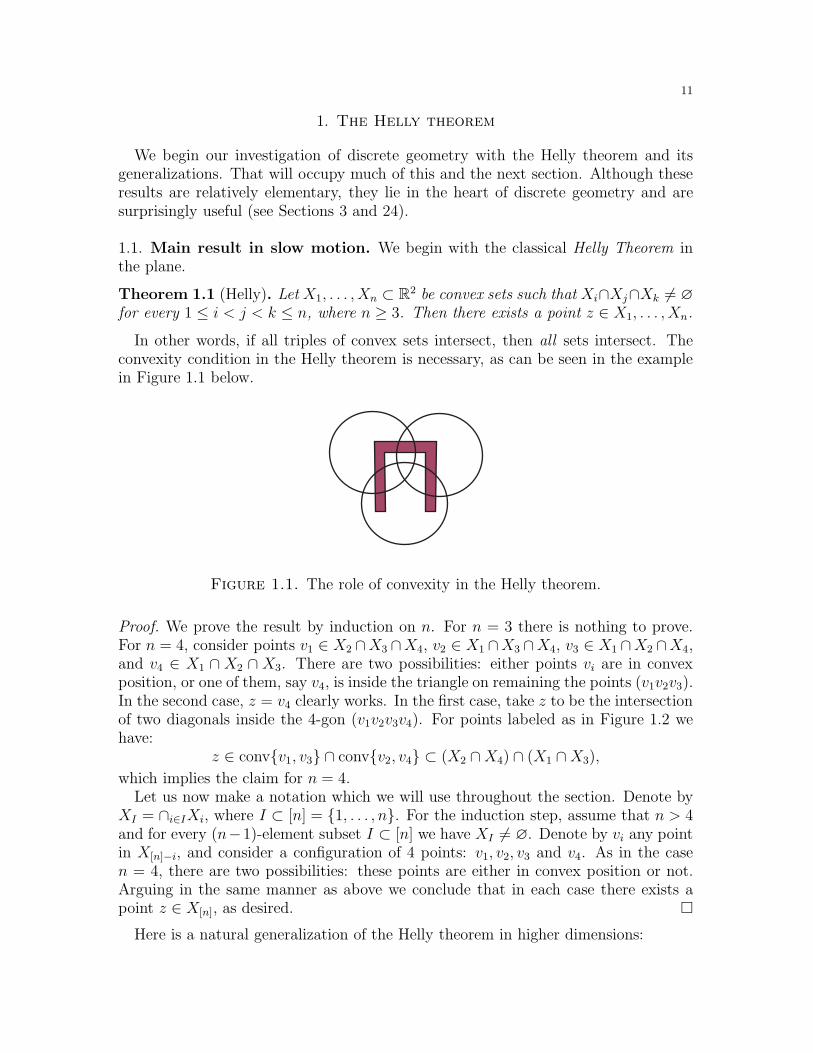
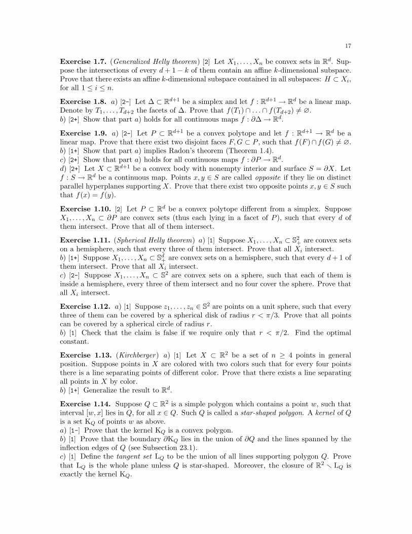
In other words, if all triples of convex sets intersect, then all sets intersect. Theconvexity condition in the Helly theorem is necessary, as can be seen in the examplein Figure 1.1 below.

Figure 1.1. The role of convexity in the Helly theorem.

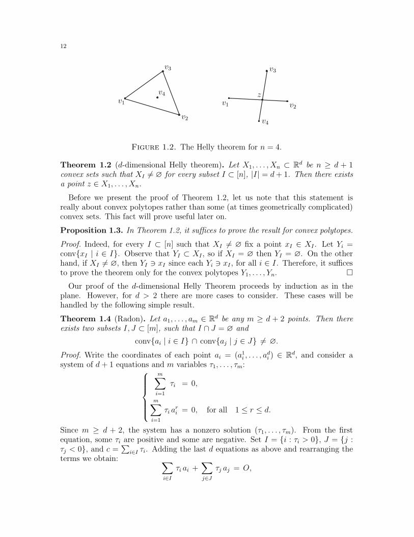
Proof. We prove the result by induction on n. For n = 3 there is nothing to prove.For n = 4, consider points v1 ∈ X2 ∩X3 ∩X4, v2 ∈ X1 ∩X3 ∩X4, v3 ∈ X1 ∩X2 ∩X4,and v4 ∈ X1 ∩ X2 ∩ X3. There are two possibilities: either points vi are in convexposition, or one of them, say v4, is inside the triangle on remaining the points (v1v2v3).In the second case, z = v4 clearly works. In the first case, take z to be the intersectionof two diagonals inside the 4-gon (v1v2v3v4). For points labeled as in Figure 1.2 wehave:

z ∈ convv1, v3 ∩ convv2, v4 ⊂ (X2 ∩X4) ∩ (X1 ∩X3),

which implies the claim for n = 4.Let us now make a notation which we will use throughout the section. Denote by

XI = ∩i∈IXi, where I ⊂ [n] = 1, . . . , n. For the induction step, assume that n > 4and for every (n−1)-element subset I ⊂ [n] we have XI 6= ∅. Denote by vi any pointin X[n]−i, and consider a configuration of 4 points: v1, v2, v3 and v4. As in the casen = 4, there are two possibilities: these points are either in convex position or not.Arguing in the same manner as above we conclude that in each case there exists apoint z ∈ X[n], as desired.

Here is a natural generalization of the Helly theorem in higher dimensions:

12

v1v1 v2

v2

v3v3

v4

v4 z

Figure 1.2. The Helly theorem for n = 4.

Theorem 1.2 (d-dimensional Helly theorem). Let X1, . . . , Xn ⊂ Rd be n ≥ d + 1convex sets such that XI 6= ∅ for every subset I ⊂ [n], |I| = d+ 1. Then there existsa point z ∈ X1, . . . , Xn.

Before we present the proof of Theorem 1.2, let us note that this statement isreally about convex polytopes rather than some (at times geometrically complicated)convex sets. This fact will prove useful later on.

Proposition 1.3. In Theorem 1.2, it suffices to prove the result for convex polytopes.

Proof. Indeed, for every I ⊂ [n] such that XI 6= ∅ fix a point xI ∈ XI . Let Yi =convxI | i ∈ I. Observe that YI ⊂ XI , so if XI = ∅ then YI = ∅. On the otherhand, if XI 6= ∅, then YI ∋ xI since each Yi ∋ xI , for all i ∈ I. Therefore, it sufficesto prove the theorem only for the convex polytopes Y1, . . . , Yn.

Our proof of the d-dimensional Helly Theorem proceeds by induction as in theplane. However, for d > 2 there are more cases to consider. These cases will behandled by the following simple result.

Theorem 1.4 (Radon). Let a1, . . . , am ∈ Rd be any m ≥ d + 2 points. Then thereexists two subsets I, J ⊂ [m], such that I ∩ J = ∅ and

convai | i ∈ I ∩ convaj | j ∈ J 6= ∅.

Proof. Write the coordinates of each point ai = (a1i , . . . , a

di ) ∈ Rd, and consider a

system of d+ 1 equations and m variables τ1, . . . , τm:

m∑

i=1

τi = 0,

m∑

i=1

τi ari = 0, for all 1 ≤ r ≤ d.

Since m ≥ d + 2, the system has a nonzero solution (τ1, . . . , τm). From the firstequation, some τi are positive and some are negative. Set I = i : τi > 0, J = j :τj < 0, and c =

∑i∈I τi. Adding the last d equations as above and rearranging the

terms we obtain: ∑

i∈Iτi ai +

∑

j∈Jτj aj = O,

13

∑

i∈I

τicai =

∑

j∈J

−τjc

aj .

Since both sides are convex combinations of points ai from disjoint sets I and J , weobtain the result.

Proof of Theorem 1.2. Use induction. The case n = d+1 is clear. Suppose n ≥ d+2and every (n− 1)-element subset of convex sets Xi has a common point vi ∈ X[n]−i.By Radon’s theorem, there exists two disjoint subsets I, J ⊂ [n] and a point z ∈ Rd,such that

z ∈ convvi | i ∈ I ∩ convvj | j ∈ J ⊂ X[n]rI ∩ X[n]rJ ⊂ X[n] ,

where the second inclusion follows by definition of points vi.

1.2. Softball geometric applications. The Helly theorem does not look at allpowerful, but it has, in fact, a number of nice geometric applications. We presenthere several such applications, leaving others as exercises.

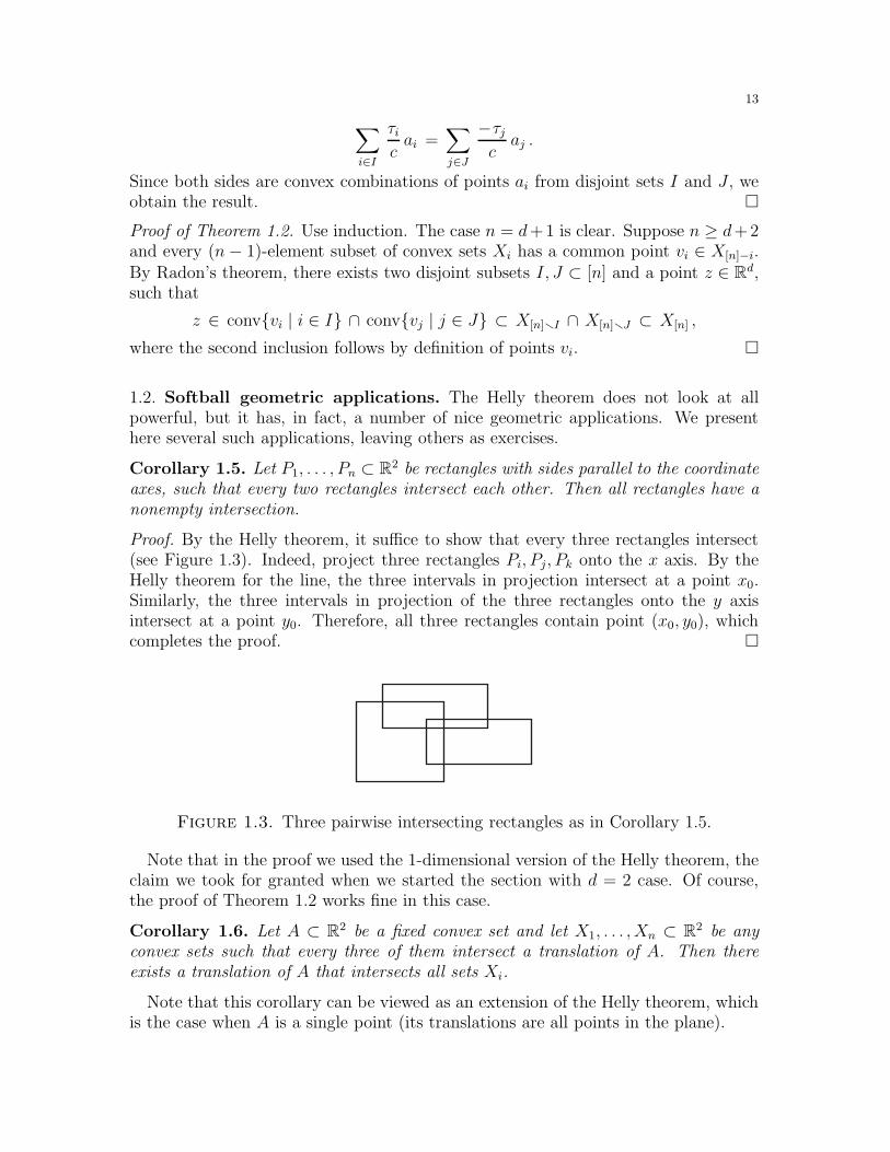
Corollary 1.5. Let P1, . . . , Pn ⊂ R2 be rectangles with sides parallel to the coordinateaxes, such that every two rectangles intersect each other. Then all rectangles have anonempty intersection.

Proof. By the Helly theorem, it suffice to show that every three rectangles intersect(see Figure 1.3). Indeed, project three rectangles Pi, Pj, Pk onto the x axis. By theHelly theorem for the line, the three intervals in projection intersect at a point x0.Similarly, the three intervals in projection of the three rectangles onto the y axisintersect at a point y0. Therefore, all three rectangles contain point (x0, y0), whichcompletes the proof.

Figure 1.3. Three pairwise intersecting rectangles as in Corollary 1.5.

Note that in the proof we used the 1-dimensional version of the Helly theorem, theclaim we took for granted when we started the section with d = 2 case. Of course,the proof of Theorem 1.2 works fine in this case.

Corollary 1.6. Let A ⊂ R2 be a fixed convex set and let X1, . . . , Xn ⊂ R2 be anyconvex sets such that every three of them intersect a translation of A. Then thereexists a translation of A that intersects all sets Xi.

Note that this corollary can be viewed as an extension of the Helly theorem, whichis the case when A is a single point (its translations are all points in the plane).

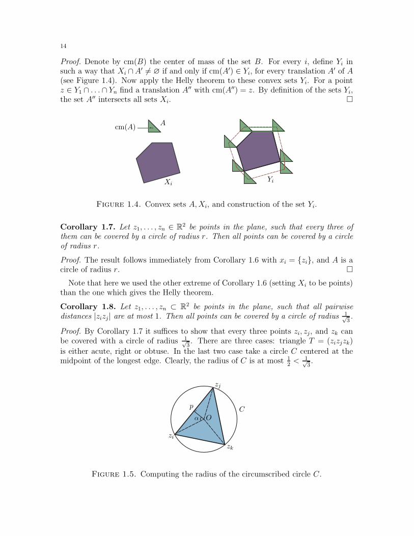
14

Proof. Denote by cm(B) the center of mass of the set B. For every i, define Yi insuch a way that Xi ∩A′ 6= ∅ if and only if cm(A′) ∈ Yi, for every translation A′ of A(see Figure 1.4). Now apply the Helly theorem to these convex sets Yi. For a pointz ∈ Y1 ∩ . . . ∩ Yn find a translation A′′ with cm(A′′) = z. By definition of the sets Yi,the set A′′ intersects all sets Xi.

Acm(A)

XiYi

Figure 1.4. Convex sets A,Xi, and construction of the set Yi.

Corollary 1.7. Let z1, . . . , zn ∈ R2 be points in the plane, such that every three ofthem can be covered by a circle of radius r. Then all points can be covered by a circleof radius r.

Proof. The result follows immediately from Corollary 1.6 with xi = zi, and A is acircle of radius r.

Note that here we used the other extreme of Corollary 1.6 (setting Xi to be points)than the one which gives the Helly theorem.

Corollary 1.8. Let z1, . . . , zn ⊂ R2 be points in the plane, such that all pairwisedistances |zizj| are at most 1. Then all points can be covered by a circle of radius 1√

3.

Proof. By Corollary 1.7 it suffices to show that every three points zi, zj, and zk canbe covered with a circle of radius 1√

3. There are three cases: triangle T = (zizjzk)

is either acute, right or obtuse. In the last two case take a circle C centered at themidpoint of the longest edge. Clearly, the radius of C is at most 1

2< 1√

3.

C

zi

zj

zk

O

p

α

Figure 1.5. Computing the radius of the circumscribed circle C.

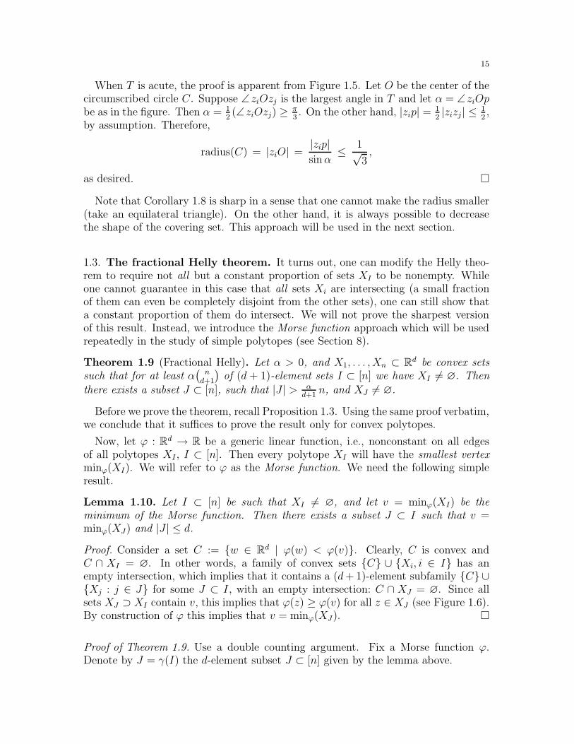
15

When T is acute, the proof is apparent from Figure 1.5. Let O be the center of thecircumscribed circle C. Suppose ∠ ziOzj is the largest angle in T and let α = ∠ ziOpbe as in the figure. Then α = 1

2(∠ ziOzj) ≥ π

3. On the other hand, |zip| = 1

2|zizj | ≤ 1

2,

by assumption. Therefore,

radius(C) = |ziO| =|zip|sinα

≤ 1√3,

as desired.

Note that Corollary 1.8 is sharp in a sense that one cannot make the radius smaller(take an equilateral triangle). On the other hand, it is always possible to decreasethe shape of the covering set. This approach will be used in the next section.

1.3. The fractional Helly theorem. It turns out, one can modify the Helly theo-rem to require not all but a constant proportion of sets XI to be nonempty. Whileone cannot guarantee in this case that all sets Xi are intersecting (a small fractionof them can even be completely disjoint from the other sets), one can still show thata constant proportion of them do intersect. We will not prove the sharpest versionof this result. Instead, we introduce the Morse function approach which will be usedrepeatedly in the study of simple polytopes (see Section 8).

Theorem 1.9 (Fractional Helly). Let α > 0, and X1, . . . , Xn ⊂ Rd be convex setssuch that for at least α

(nd+1

)of (d + 1)-element sets I ⊂ [n] we have XI 6= ∅. Then

there exists a subset J ⊂ [n], such that |J | > αd+1

n, and XJ 6= ∅.

Before we prove the theorem, recall Proposition 1.3. Using the same proof verbatim,we conclude that it suffices to prove the result only for convex polytopes.

Now, let ϕ : Rd → R be a generic linear function, i.e., nonconstant on all edgesof all polytopes XI , I ⊂ [n]. Then every polytope XI will have the smallest vertexminϕ(XI). We will refer to ϕ as the Morse function. We need the following simpleresult.

Lemma 1.10. Let I ⊂ [n] be such that XI 6= ∅, and let v = minϕ(XI) be theminimum of the Morse function. Then there exists a subset J ⊂ I such that v =minϕ(XJ) and |J | ≤ d.

Proof. Consider a set C := w ∈ Rd | ϕ(w) < ϕ(v). Clearly, C is convex andC ∩ XI = ∅. In other words, a family of convex sets C ∪ Xi, i ∈ I has anempty intersection, which implies that it contains a (d+ 1)-element subfamily C ∪Xj : j ∈ J for some J ⊂ I, with an empty intersection: C ∩ XJ = ∅. Since allsets XJ ⊃ XI contain v, this implies that ϕ(z) ≥ ϕ(v) for all z ∈ XJ (see Figure 1.6).By construction of ϕ this implies that v = minϕ(XJ).

Proof of Theorem 1.9. Use a double counting argument. Fix a Morse function ϕ.Denote by J = γ(I) the d-element subset J ⊂ [n] given by the lemma above.

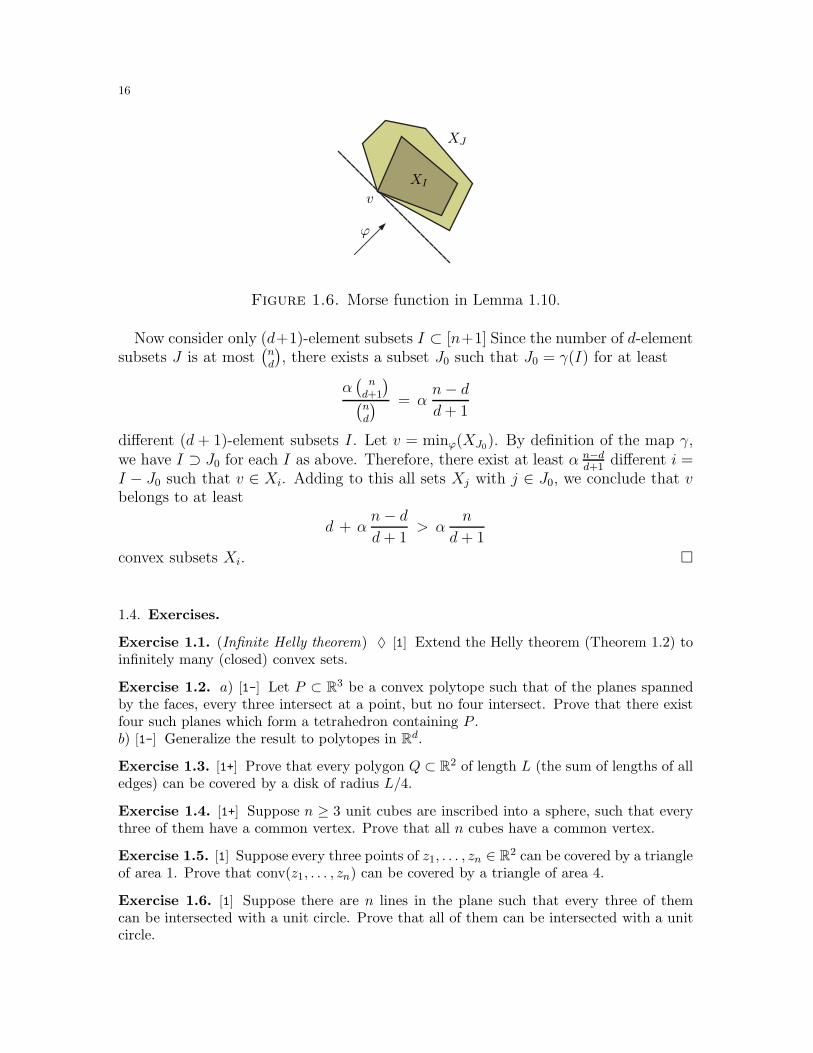
16

ϕ

v

XI

XJ

Figure 1.6. Morse function in Lemma 1.10.

Now consider only (d+1)-element subsets I ⊂ [n+1] Since the number of d-elementsubsets J is at most

(nd

), there exists a subset J0 such that J0 = γ(I) for at least

α(nd+1

)(nd

) = αn− dd+ 1

different (d + 1)-element subsets I. Let v = minϕ(XJ0). By definition of the map γ,

we have I ⊃ J0 for each I as above. Therefore, there exist at least α n−dd+1

different i =I − J0 such that v ∈ Xi. Adding to this all sets Xj with j ∈ J0, we conclude that vbelongs to at least

d + αn− dd+ 1

> αn

d+ 1

convex subsets Xi.

1.4. Exercises.

Exercise 1.1. (Infinite Helly theorem) ♦ [1] Extend the Helly theorem (Theorem 1.2) toinfinitely many (closed) convex sets.

Exercise 1.2. a) [1-] Let P ⊂ R3 be a convex polytope such that of the planes spannedby the faces, every three intersect at a point, but no four intersect. Prove that there existfour such planes which form a tetrahedron containing P .b) [1-] Generalize the result to polytopes in Rd.

Exercise 1.3. [1+] Prove that every polygon Q ⊂ R2 of length L (the sum of lengths of alledges) can be covered by a disk of radius L/4.

Exercise 1.4. [1+] Suppose n ≥ 3 unit cubes are inscribed into a sphere, such that everythree of them have a common vertex. Prove that all n cubes have a common vertex.

Exercise 1.5. [1] Suppose every three points of z1, . . . , zn ∈ R2 can be covered by a triangleof area 1. Prove that conv(z1, . . . , zn) can be covered by a triangle of area 4.

Exercise 1.6. [1] Suppose there are n lines in the plane such that every three of themcan be intersected with a unit circle. Prove that all of them can be intersected with a unitcircle.

17

Exercise 1.7. (Generalized Helly theorem) [2] Let X1, . . . ,Xn be convex sets in Rd. Sup-pose the intersections of every d+ 1− k of them contain an affine k-dimensional subspace.Prove that there exists an affine k-dimensional subspace contained in all subspaces: H ⊂ Xi,for all 1 ≤ i ≤ n.

Exercise 1.8. a) [2-] Let ∆ ⊂ Rd+1 be a simplex and let f : Rd+1 → Rd be a linear map.Denote by T1, . . . , Td+2 the facets of ∆. Prove that f(T1) ∩ . . . ∩ f(Td+2) 6= ∅.b) [2+] Show that part a) holds for all continuous maps f : ∂∆→ Rd.

Exercise 1.9. a) [2-] Let P ⊂ Rd+1 be a convex polytope and let f : Rd+1 → Rd be alinear map. Prove that there exist two disjoint faces F,G ⊂ P , such that f(F )∩ f(G) 6= ∅.b) [1+] Show that part a) implies Radon’s theorem (Theorem 1.4).c) [2+] Show that part a) holds for all continuous maps f : ∂P → Rd.d) [2+] Let X ⊂ Rd+1 be a convex body with nonempty interior and surface S = ∂X. Letf : S → Rd be a continuous map. Points x, y ∈ S are called opposite if they lie on distinctparallel hyperplanes supporting X. Prove that there exist two opposite points x, y ∈ S suchthat f(x) = f(y).

Exercise 1.10. [2] Let P ⊂ Rd be a convex polytope different from a simplex. SupposeX1, . . . ,Xn ⊂ ∂P are convex sets (thus each lying in a facet of P ), such that every d ofthem intersect. Prove that all of them intersect.

Exercise 1.11. (Spherical Helly theorem) a) [1] Suppose X1, . . . ,Xn ⊂ S2+ are convex sets

on a hemisphere, such that every three of them intersect. Prove that all Xi intersect.b) [1+] Suppose X1, . . . ,Xn ⊂ Sd+ are convex sets on a hemisphere, such that every d+ 1 ofthem intersect. Prove that all Xi intersect.c) [2-] Suppose X1, . . . ,Xn ⊂ S2 are convex sets on a sphere, such that each of them isinside a hemisphere, every three of them intersect and no four cover the sphere. Prove thatall Xi intersect.

Exercise 1.12. a) [1] Suppose z1, . . . , zn ∈ S2 are points on a unit sphere, such that everythree of them can be covered by a spherical disk of radius r < π/3. Prove that all pointscan be covered by a spherical circle of radius r.b) [1] Check that the claim is false if we require only that r < π/2. Find the optimalconstant.

Exercise 1.13. (Kirchberger) a) [1] Let X ⊂ R2 be a set of n ≥ 4 points in generalposition. Suppose points in X are colored with two colors such that for every four pointsthere is a line separating points of different color. Prove that there exists a line separatingall points in X by color.b) [1+] Generalize the result to Rd.

Exercise 1.14. Suppose Q ⊂ R2 is a simple polygon which contains a point w, such thatinterval [w, x] lies in Q, for all x ∈ Q. Such Q is called a star-shaped polygon. A kernel of Qis a set KQ of points w as above.a) [1-] Prove that the kernel KQ is a convex polygon.b) [1] Prove that the boundary ∂KQ lies in the union of ∂Q and the lines spanned by theinflection edges of Q (see Subsection 23.1).c) [1] Define the tangent set LQ to be the union of all lines supporting polygon Q. Provethat LQ is the whole plane unless Q is star-shaped. Moreover, the closure of R2 r LQ isexactly the kernel KQ.

18

d) [1+] For a 2-dimensional polyhedral surface S ⊂ R3 define the tangent set LS to be theunion of planes tangent to S. Prove that LS = R3 unless S is homeomorphic to a sphereand encloses a star-shaped 3-dimensional polyhedron.

Exercise 1.15. (Krasnosel’skii) a) [1] Suppose Q ⊂ R2 is a simple polygon, such thatfor every three points x, y, z ∈ Q there exists a point v such that line segments [vx], [vy],and [vz] lie in Q. Prove that Q is a star-shaped polygon.b) [1+] Generalize the result to Rd; use (d+ 1)-tuples of points.

Exercise 1.16. a) [2-] Let X1, . . . ,Xm ⊂ Rd be convex sets such that their union is alsoconvex. Prove that if every m− 1 of them intersect, then all of them intersect.b) [2] Let X1, . . . ,Xm ⊂ Rd be convex sets such that the union of every d + 1 or fewer ofthem is a star-shaped region. Then all Xi have a nonempty intersection.c) [2-] Deduce part a) from part b).d) [2+] Find a ‘fractional analogue’ of part b).

Exercise 1.17. a) [1] Let Q ⊂ R2 be a union of axis parallel rectangles. Suppose for everytwo points x, y ∈ Q there exists a point v ∈ Q, such that line segments [vx] and [vy] liein Q. Prove that Q is a star-shaped polygon.b) [1+] Generalize the result to Rd; use pairs of points.

Exercise 1.18. a) [2-] Suppose X1, . . . ,Xn ⊂ R2 are disks such that every two of themintersect. Prove that there exist four points z1, . . . , z4 such that every Xi contains at leastone zj .b) [2-] In condition of a), suppose Xi are unit disks. Prove that three points zj suffice.

Exercise 1.19. [1+] Prove that for every finite set of n points X ⊂ R2 there exist at most ndisks which cover X, such that the distance between any two disks is ≥ 1, and the totaldiameter is ≤ n.

Exercise 1.20. a) [2-] Suppose X1, . . . ,Xn ⊂ R2 are convex sets such that through everyfour of them there exists a line intersecting them. Prove that there exist two lines ℓ1 and ℓ2such that every Xi intersects ℓ1 or ℓ2.b) [2+] LetX1, . . . ,Xn ⊂ Rd be axis parallel bricks. Suppose for any (d+1)2d−1 of these thereexists a hyperplane intersecting them. Prove that there exists a hyperplane intersectingall Xi, 1 ≤ i ≤ n.

Exercise 1.21. (Topological Helly theorem) a) [1] Let X1, . . . ,Xn ⊂ R2 be simple poly-gons3 in the plane, such that all double and triple intersections of Xi are also (nonempty)simple polygons. Prove that the intersection of all Xi is also a simple polygon.b) [1+] Generalize part a) to higher dimensions.

Exercise 1.22. a) [1] Let X1, . . . ,Xn ⊂ R2 be simple polygons in the plane, by which wemean here polygonal regions with no holes. Suppose that all unions Xi∪Xj are also simplepolygons, and that all intersections Xi ∩Xj are nonempty. Prove that the intersection ofall Xi is also nonempty.b) [1+] LetX1, . . . ,Xn ⊂ R2 be simple polygons in the plane, such that all unionsXi∪Xj∪Xk

are also simple, for all 1 ≤ i ≤ j ≤ k ≤ n. Prove that the intersection of all Xi is nonempty.

Exercise 1.23. (Weak converse Helly theorem) a) [1] Let X ⊂ R2 be a simple polygonsuch that for every collection of triangles T1, . . . , Tn ⊂ R2 either X ∩ T1 ∩ · · · ∩ Tn 6= ∅, orX ∩ Ti ∩ Tj = ∅ for some 1 ≤ i < j < n. Prove that X is convex.

3Here a simple polygon is a connected, simply connected finite union of convex polygons.

19

b) [1+] Generalize part a) to higher dimensions.

Exercise 1.24. (Converse Helly theorem) a) [2-] Let A be an infinite family of simplepolygons in the plane which is closed under non-degenerate affine transformations. Sup-pose A satisfies the following property: for every four elements in A, if every three of themintersect, then so does the fourth. Prove that all polygons in A are convex.b) [2] Extend this to general compact sets in the plane.c) [2+] Generalize this to higher dimensions.

Exercise 1.25. (Convexity criterion) ♦ a) [2-] Let X ⊂ R3 be a compact set and supposeevery intersection of X by a plane is contractible. Prove that X is convex.4

b) [2+] Generalize this to higher dimensions.

Exercise 1.26. a) [2-] Let A be an infinite family of simple polygons in the plane whichis closed under rigid motions and intersections. Prove that all polygons in A are convex.b) [2] Extend this to general connected compact sets in the plane.c) [2] Generalize this to higher dimensions.

1.5. Final remarks. For a classical survey on the Helly theorem and its applications werefer to [DGK]. See also [Eck] for recent results and further references. The corollaries wepresent in this section are selected from [HDK] where numerous other applications of Hellytheorem are presented as exercises.

Our proof of the fractional Helly theorem (Theorem 1.9) with minor modifications fol-lows [Mat1, §8.1]. The constant α/(d+ 1) in the theorem can be replaced with the optimalconstant

1− (1− α)1/(d+1),

due to Gil Kalai (see [Eck] for references and discussions of this and related results).

4Already the case when X is polyhedral (a finite union of convex polytopes) is non-trivial and isa good starting point.

20

2. Caratheodory and Barany theorems

This short section is a followup of the previous section. The main result, the Baranytheorem, is a stand-alone result simply too beautiful to be missed. Along the waywe prove the classical Sylvester–Gallai theorem, the first original result in the wholesubfield of point and line configurations (see Section 12).

2.1. Triangulations are fun. We start by stating the following classical theorem inthe case of a finite set of points.

Theorem 2.1 (Caratheodory). Let X ⊂ Rd be a finite set of points, and let z ∈conv(X). Then there exist x1, . . . , xd+1 ∈ X such that z ∈ convx1, . . . , xd+1.

Of the many easy proofs of the theorem, the one most relevant to the subject is the‘proof by triangulation’: given a simplicial triangulation of a convex polytope P =conv(X), take any simplex containing z (there may be more than one). To obtain atriangulation of a convex polytope, choose a vertex v ∈ P and triangulate all facetsof P (use induction on the dimension). Then consider all cones from v to the simplicesin the facet triangulations.5

One can also ask how many simplices with vertices in X can contain the samepoint. While this number may vary depending on the location of the point, it turnsout there always exists a point z which is contained in a constant proportion of allsimplices.

Theorem 2.2 (Barany). For every d ≥ 1 there exists a constant αd > 0, such thatfor every set of n points X ⊂ Rd in general position, there exists a point z ∈ conv(X)contained in at least αd

(nd+1

)simplices (x1 . . . xd+1), xi ∈ X.

Here the points are in general position if no three points lie on a line. This resultis nontrivial even for convex polygons in the plane, where the triangulations are wellunderstood. We suggest the reader try to prove the result in this special case beforegoing through the proof below.

2.2. Infinite descent as a mathematical journey. The method of infinite descentis a basic tool in mathematics, with a number of applications in geometry. To illus-trate the method and prepare for the proof of the Barany theorem we start with thefollowing classical result of independent interest:

Theorem 2.3 (Sylvester–Gallai). Let X ∈ R2 be a finite set of points, not all on thesame line. Then there exists a line containing exactly two points in X.

Proof. Suppose every line which goes through two points in X, goes also through athird such point. Since the total number of such lines is finite, consider the shortestdistance between points and lines. Suppose the minimum is achieved at a pair:point y ∈ X and line ℓ. Suppose also that ℓ goes through points x1, x2, x3 (in that

5Formally speaking, in dimensions at least 4, this argument produces a dissection, and not neces-sarily a (face-to-face) triangulation (see Exercise 2.1). Of course, a dissection suffices for the purposesof the Caratheodory theorem. We formalize and extend this approach in Subsection 14.5.

21

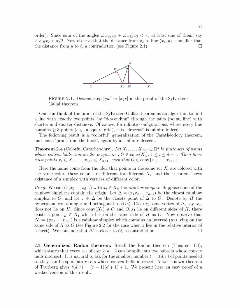
order). Since sum of the angles ∠x1yx2 + ∠x2yx3 < π, at least one of them, say∠x1yx2 < π/2. Now observe that the distance from x2 to line (x1, y) is smaller thatthe distance from y to ℓ, a contradiction (see Figure 2.1).

x1 x2 x3

y

v

w

Figure 2.1. Descent step [yw]→ [x2v] in the proof of the Sylvester–Gallai theorem.

One can think of the proof of the Sylvester–Gallai theorem as an algorithm to finda line with exactly two points, by “descending” through the pairs (point, line) withshorter and shorter distances. Of course, for infinite configurations, where every linecontains ≥ 3 points (e.g., a square grid), this “descent” is infinite indeed.

The following result is a “colorful” generalization of the Caratheodory theorem,and has a ‘proof from the book’, again by an infinite descent.

Theorem 2.4 (Colorful Caratheodory). Let X1, . . . , Xd+1 ⊂ Rd be finite sets of pointswhose convex hulls contain the origin, i.e., O ∈ conv(Xi), 1 ≤ i ≤ d+ 1. Then thereexist points x1 ∈ X1, . . . , xd+1 ∈ Xd+1, such that O ∈ convx1, . . . , xd+1.

Here the name come from the idea that points in the same set Xi are colored withthe same color, these colors are different for different Xi, and the theorem showsexistence of a simplex with vertices of different color.

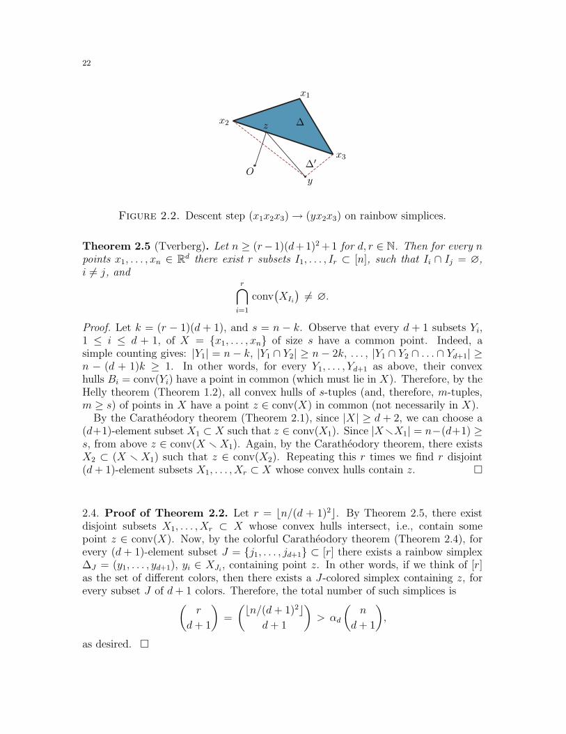
Proof. We call (x1x2 . . . xd+1) with xi ∈ Xi, the rainbow simplex. Suppose none of therainbow simplices contain the origin. Let ∆ = (x1x2 . . . xd+1) be the closest rainbowsimplex to O, and let z ∈ ∆ be the closets point of ∆ to O. Denote by H thehyperplane containing z and orthogonal to (Oz). Clearly, some vertex of ∆, say, x1,does not lie on H . Since conv(X1) ∋ O and O, x1 lie on different sides of H , thereexists a point y ∈ X1 which lies on the same side of H as O. Now observe that∆′ := (yx2 . . . xd+1) is a rainbow simplex which contains an interval (yz) lying on thesame side of H as O (see Figure 2.2 for the case when z lies in the relative interior ofa facet). We conclude that ∆′ is closer to O, a contradiction.

2.3. Generalized Radon theorem. Recall the Radon theorem (Theorem 1.4),which states that every set of size ≥ d+2 can be split into two subsets whose convexhulls intersect. It is natural to ask for the smallest number t = t(d, r) of points neededso they can be split into r sets whose convex hulls intersect. A well known theoremof Tverberg gives t(d, r) = (r − 1)(d + 1) + 1. We present here an easy proof of aweaker version of this result.

22

x1

x2

x3

y

z ∆

∆′O

Figure 2.2. Descent step (x1x2x3)→ (yx2x3) on rainbow simplices.

Theorem 2.5 (Tverberg). Let n ≥ (r−1)(d+1)2 +1 for d, r ∈ N. Then for every npoints x1, . . . , xn ∈ Rd there exist r subsets I1, . . . , Ir ⊂ [n], such that Ii ∩ Ij = ∅,i 6= j, and

r⋂

i=1

conv(XIi

)6= ∅.

Proof. Let k = (r − 1)(d + 1), and s = n − k. Observe that every d + 1 subsets Yi,1 ≤ i ≤ d + 1, of X = x1, . . . , xn of size s have a common point. Indeed, asimple counting gives: |Y1| = n− k, |Y1 ∩ Y2| ≥ n− 2k, . . . , |Y1 ∩ Y2 ∩ . . . ∩ Yd+1| ≥n − (d + 1)k ≥ 1. In other words, for every Y1, . . . , Yd+1 as above, their convexhulls Bi = conv(Yi) have a point in common (which must lie in X). Therefore, by theHelly theorem (Theorem 1.2), all convex hulls of s-tuples (and, therefore, m-tuples,m ≥ s) of points in X have a point z ∈ conv(X) in common (not necessarily in X).

By the Caratheodory theorem (Theorem 2.1), since |X| ≥ d + 2, we can choose a(d+1)-element subset X1 ⊂ X such that z ∈ conv(X1). Since |XrX1| = n−(d+1) ≥s, from above z ∈ conv(X rX1). Again, by the Caratheodory theorem, there existsX2 ⊂ (X r X1) such that z ∈ conv(X2). Repeating this r times we find r disjoint(d+ 1)-element subsets X1, . . . , Xr ⊂ X whose convex hulls contain z.

2.4. Proof of Theorem 2.2. Let r = ⌊n/(d + 1)2⌋. By Theorem 2.5, there existdisjoint subsets X1, . . . , Xr ⊂ X whose convex hulls intersect, i.e., contain somepoint z ∈ conv(X). Now, by the colorful Caratheodory theorem (Theorem 2.4), forevery (d + 1)-element subset J = j1, . . . , jd+1 ⊂ [r] there exists a rainbow simplex∆J = (y1, . . . , yd+1), yi ∈ XJi

, containing point z. In other words, if we think of [r]as the set of different colors, then there exists a J-colored simplex containing z, forevery subset J of d+ 1 colors. Therefore, the total number of such simplices is

(r

d+ 1

)=

(⌊n/(d+ 1)2⌋d+ 1

)> αd

(n

d+ 1

),

as desired.

23

2.5. Exercises.

Exercise 2.1. ♦ [1-] Check that the argument below Theorem 2.1 produces a (face-to-face)triangulation in R3. Explain what can go wrong in R4.

Exercise 2.2. (Dual Sylvester–Gallai theorem) [1] Let L be a finite set of lines in the plane,not all going through the same point. Prove that there exists a point x ∈ R2 contained inexactly two lines.

Exercise 2.3. ♦ a) [1] Let L be a finite set of lines in the plane, not all going through thesame point. Denote by pi the number of points which lie in exactly i lines, and by qi thenumber of regions in the plane (separated by L) with i sides. Prove:

∑

i≥2

(3− i)pi +∑

i≥3

(3− i)qi = 3

Conclude from here that p2 ≥ 3, implying the dual Sylvester–Gallai theorem.b) [1] Use combinatorial duality “points ↔ lines” to similarly show that for a finite set ofpoints, not all on the same line, there exists at least three lines, each containing exactly twopoints.

Exercise 2.4. (Graham–Newman problem) [2-] Let X ∈ R2 be a finite set of points, not allon the same line. Suppose the points are colored with two colors. A line is called monochro-matic if all its points in X have the same color. Prove that there exists a monochromaticline containing at least two points in X.

Exercise 2.5. [1] Let X = x1, . . . , xn ⊂ R2 be a finite set of points, not all on the sameline. Suppose real numbers a1, . . . , an are associated with the points such that the sumalong every line is zero. Prove that all numbers are zero.

Exercise 2.6. [1] Let X1, . . . ,Xn ⊂ Rd be any convex sets, and z ∈ conv(X1 ∪ . . . ∪Xn).Then there exist a subset I ⊂ [n], |I| = d+ 1, such that z ∈ conv (∪i∈IXi).

Exercise 2.7. [1+] Let P ⊂ Rd be a simple polytope with m facets. Fix n = m−d verticesv1, . . . , vn. Then there exists a vertex w and facets F1, . . . , Fn ⊂ P , such that w, vi /∈ Fi,for all 1 ≤ i ≤ n.

Exercise 2.8. (Steinitz ) a) [1+] Let X ⊂ Rd be a finite set of points, let P = conv(X) andlet z ∈ P r∂P be a point in the interior of P . Then there exists a subset Y ⊂ X, |Y | ≤ 2d,such that z ∈ Qr ∂Q is the point in the interior of Q = conv(Y ).6

b) [1-] Show that the upper bound |Y | ≤ 2d is tight.

Exercise 2.9. a) [2-] Let X1, . . . ,Xn be convex sets in Rd such that the intersection ofevery 2d of them has volume ≥ 1. Then the intersection of all Xi has volume ≥ c, wherec = c(d) > 0 is a universal constant which depends only on d.b) [1-] Check that the number 2d cannot be lowered.

Exercise 2.10. a) [1-] Suppose points x1, x2 and x3 are chosen uniformly and indepen-dently at random from the unit circle centered at the origin O. Show that the probabilitythat O ∈ (x1x2x3) is equal to 1/4.b) [1+] Generalize part a) to higher dimensions.

6Think of this result as a variation on the Caratheodory theorem.

24

Exercise 2.11. [1] Let X = [x1 . . . xn] ⊂ R2 be a convex polygon. Prove that there existn−2 points y1, . . . , yn−2 ⊂ R2 such that every triangle on X contains at least one point yi.

7

Show that this is impossible to do with fewer than n− 2 points.

Exercise 2.12. Let P ⊂ R3 be a convex polytope of volume 1. Suppose X ⊂ P is a setof n points.a) [1-] Prove that there exists a convex polytope Q ⊂ P rX such that vol(Q) ≥ 1

n .

b) [1+] For every n = 3(2k − 1), prove that there exists a convex polytope Q ⊂ P rX suchthat vol(Q) ≥ 2−k.

Exercise 2.13. (Cone triangulation) [1] Let C ⊂ Rd be a convex cone, defined as theintersection of finitely many halfspaces containing the origin O. A cone in Rd is calledsimple if it has d faces. Prove that C can be subdivided into convex cones.

Exercise 2.14. a) [1+] Let Q ⊂ R3 be a space polygon, and let P ⊂ R3 be the convex hullof Q. Prove that every point v ∈ P belongs to a triangle with vertices in Q.b) [2-] Extend this result to Rd and general connected sets Q.

Exercise 2.15. [2+] We say that a polygon Q ⊂ R2d is convex if every hyperplane intersectsit at most 2d times. Denote by P the convex hull of Q. Prove that every point v ∈ P belongsto a d-simplex with vertices in Q.

Exercise 2.16. Let P ⊂ Rd be a convex polytope with n facets, and let X = x1, . . . , xnbe a fixed subset of interior points in P . For a facet F of P and a vertex xi, define a pyramidΦi(F ) = conv(F, xi).a) [2] Prove that one can label the facets F1, . . . , Fd in such a way that pyramids Φi(Fi) donot intersect except at the boundaries.b) [2] Prove that one can label the facets F1, . . . , Fd in such way that the pyramids Φi(Fi)cover the whole P .

Exercise 2.17. (Colorful Helly theorem) [2-] Let F1, . . . ,Fd+1 be finite families of convexsets in Rd. Suppose for every X1 ∈ F1, . . . , Xd+1 ∈ Fd+1 we have X1 ∩ . . . ∩ Xd+1 6= ∅.Prove that ∩X∈Fi

X 6= ∅ for some 1 ≤ i ≤ d+ 1.

Exercise 2.18. [2] Let X1, . . . ,Xd+1 ⊂ Rd be finite sets of points such that O ∈ conv(Xi∪Xj), for all 1 ≤ i < j ≤ d + 1. Then there exist points x1 ∈ X1, . . . , xd+1 ∈ Xd+1, suchthat O ∈ convx1, . . . , xd+1.

Exercise 2.19. a) [1+] Let P,Q ⊂ Rd be two convex polytopes. Prove that P ∪Q is convexif and only if every interval [vw] ⊂ P ∪Q for all vertices v of P and w of Q.b) [2] Generalize part a) to a union of n polytopes.

Exercise 2.20. a) [1] A triangle ∆ is contained in a convex, centrally symmetric polygon Q.Let ∆′ be the triangle symmetric to ∆ with respect to a point z ∈ ∆. Prove that at leastone of the vertices of ∆′ lies in Q or on its boundary.b) [1-] Extend part a) from triangles ∆ to general convex polygons.

7This immediately implies that at least one of yi is covered with at least 1

n−2

(n

3

)triangles. Obvi-

ously, this is much weaker than the constant proportion of triangles given by the Barany theorem.

25

2.6. Final remarks. The method of infinite descent is often attributed to Pythagoras andhis proof of irrationality of

√2. In the modern era it was reintroduced by Euler in his proof

of Fermat’s last theorem for the powers 3 and 4. For the history of the Sylvester–Gallaitheorem (Theorem 2.3), let us quote Paul Erdos [Erd]:

In 1933 while reading the beautiful book “Anschauliche Geometrie” of Hilbertand Cohn–Vossen [HilC], the following pretty conjecture occurred to me: Letx1, . . . , xn, be a finite set of points in the plane not all on a line. Then therealways is a line which goes through exactly two of the points. I expected thisto be easy but to my great surprise and disappointment I could not find aproof. I told this problem to Gallai who very soon found an ingenious proof.L. M. Kelly noticed about 10 years later that the conjecture was not new. Itwas first stated by Sylvester in the Educational Times in 1893. The first proofthough is due to Gallai.

For more on the history, variations and quantitative extensions of the Sylvester–Gallaitheorem see [ErdP, BorM], [PacA, §12] and [Mat1, §4]. We return to this result in Section 12.The method of infinite descent makes another appearance in Section 9, where it has aphysical motivation.

The Barany theorem (Theorem 2.2) and the colorful Caratheodory theorem (Theo-

rem 2.4) are due to I. Barany [Bar3]. For extensions and generalizations of results in this

section see [Mat1]. Let us mention that the exact asymptotic constant for α2 in the Barany

theorem (Theorem 2.2) is equal to 2/9. This result is due to Boros and Furedi [BorF] (see

Subsection 4.2 for the lower bound and Exercise 4.10 for the upper bound).

26

3. The Borsuk conjecture

3.1. The story in brief. Let X ⊂ Rd be a compact set, and let diam(X) denotesthe largest distance between two points in X. The celebrated Borsuk conjectureclaims that every convex set8 with diam(X) = 1 can be subdivided into d+ 1 parts,each of diameter < 1. This is known to be true for d = 2, 3. However for large d thebreakthrough result of Kahn and Kalai showed that this is spectacularly false [KahK].While we do not present the (relatively elementary) disproof of the conjecture, wewill prove the classical (now out of fashion) Borsuk theorem (the d = 2 case). Wewill also establish the Borsuk conjecture for smooth convex bodies. Finally, we use abasic topological argument to prove that three parts are not enough to subdivide thesphere S2 into parts of smaller diameter. We continue with the topological argumentsin the next three sections.

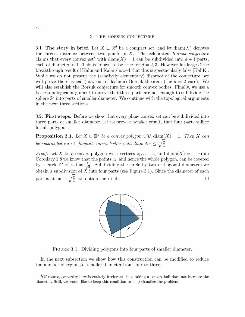
3.2. First steps. Before we show that every plane convex set can be subdivided intothree parts of smaller diameter, let us prove a weaker result, that four parts sufficefor all polygons.

Proposition 3.1. Let X ⊂ R2 be a convex polygon with diam(X) = 1. Then X can

be subdivided into 4 disjoint convex bodies with diameter ≤√

23.

Proof. Let X be a convex polygon with vertices z1, . . . , zn and diam(X) = 1. FromCorollary 1.8 we know that the points zi, and hence the whole polygon, can be coveredby a circle C of radius 1√

3. Subdividing the circle by two orthogonal diameters we

obtain a subdivision of X into four parts (see Figure 3.1). Since the diameter of each

part is at most√

23, we obtain the result.

C

X

Figure 3.1. Dividing polygons into four parts of smaller diameter.

In the next subsection we show how this construction can be modified to reducethe number of regions of smaller diameter from four to three.

8Of course, convexity here is entirely irrelevant since taking a convex hull does not increase thediameter. Still, we would like to keep this condition to help visualize the problem.

27

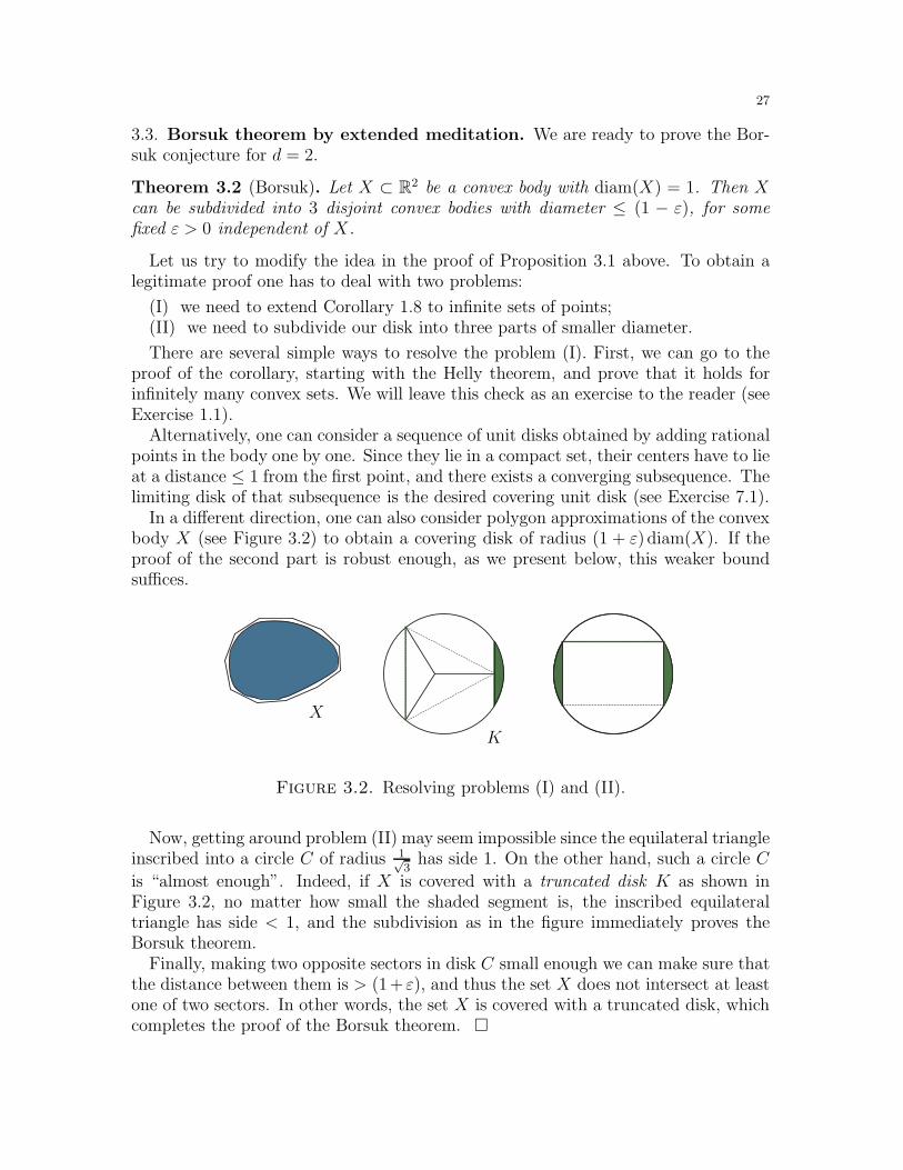
3.3. Borsuk theorem by extended meditation. We are ready to prove the Bor-suk conjecture for d = 2.

Theorem 3.2 (Borsuk). Let X ⊂ R2 be a convex body with diam(X) = 1. Then Xcan be subdivided into 3 disjoint convex bodies with diameter ≤ (1 − ε), for somefixed ε > 0 independent of X.

Let us try to modify the idea in the proof of Proposition 3.1 above. To obtain alegitimate proof one has to deal with two problems:

(I) we need to extend Corollary 1.8 to infinite sets of points;(II) we need to subdivide our disk into three parts of smaller diameter.

There are several simple ways to resolve the problem (I). First, we can go to theproof of the corollary, starting with the Helly theorem, and prove that it holds forinfinitely many convex sets. We will leave this check as an exercise to the reader (seeExercise 1.1).

Alternatively, one can consider a sequence of unit disks obtained by adding rationalpoints in the body one by one. Since they lie in a compact set, their centers have to lieat a distance ≤ 1 from the first point, and there exists a converging subsequence. Thelimiting disk of that subsequence is the desired covering unit disk (see Exercise 7.1).

In a different direction, one can also consider polygon approximations of the convexbody X (see Figure 3.2) to obtain a covering disk of radius (1 + ε) diam(X). If theproof of the second part is robust enough, as we present below, this weaker boundsuffices.

K

X

Figure 3.2. Resolving problems (I) and (II).

Now, getting around problem (II) may seem impossible since the equilateral triangleinscribed into a circle C of radius 1√

3has side 1. On the other hand, such a circle C

is “almost enough”. Indeed, if X is covered with a truncated disk K as shown inFigure 3.2, no matter how small the shaded segment is, the inscribed equilateraltriangle has side < 1, and the subdivision as in the figure immediately proves theBorsuk theorem.

Finally, making two opposite sectors in disk C small enough we can make sure thatthe distance between them is > (1+ ε), and thus the set X does not intersect at leastone of two sectors. In other words, the set X is covered with a truncated disk, whichcompletes the proof of the Borsuk theorem.

28

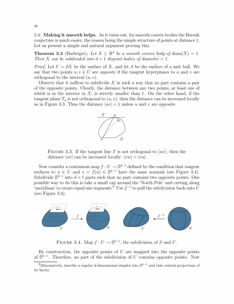
3.4. Making it smooth helps. As it turns out, for smooth convex bodies the Borsukconjecture is much easier, the reason being the simple structure of points at distance 1.Let us present a simple and natural argument proving this.

Theorem 3.3 (Hadwiger). Let X ⊂ Rd be a smooth convex body of diam(X) = 1.Then X can be subdivided into d+ 1 disjoint bodies of diameter < 1.

Proof. Let U = ∂X be the surface of X, and let S be the surface of a unit ball. Wesay that two points u, v ∈ U are opposite if the tangent hyperplanes to u and v areorthogonal to the interval (u, v).

Observe that it suffices to subdivide X in such a way that no part contains a pairof the opposite points. Clearly, the distance between any two points, at least one ofwhich is in the interior in X, is strictly smaller than 1. On the other hand, if thetangent plane Tu is not orthogonal to (u, v), then the distance can be increased locallyas in Figure 3.3. Thus the distance |uv| < 1 unless u and v are opposite.

U

u

v

wT

Figure 3.3. If the tangent line T is not orthogonal to (uv), then thedistance |uv| can be increased locally: |vw| > |vu|.

Now consider a continuous map f : U → Sd−1 defined by the condition that tangentsurfaces to u ∈ U and s = f(u) ∈ Sd−1 have the same normals (see Figure 3.4).Subdivide Sd−1 into d+ 1 parts such that no part contains two opposite points. Onepossible way to do this is take a small cap around the ‘North Pole’ and cutting along‘meridians’ to create equal size segments.9 Use f−1 to pull the subdivision back onto U(see Figure 3.4).

UU SS

f f−1

Figure 3.4. Map f : U → Sd−1, the subdivision of S and U .

By construction, the opposite points of U are mapped into the opposite pointsof Sd−1. Therefore, no part of the subdivision of U contains opposite points. Now

9Alternatively, inscribe a regular d-dimensional simplex into Sd−1 and take central projections ofits facets.

29

subdivide X by taking a cone from any interior point O ∈ X onto each part of thesubdivision of U . From the observation above, only the opposite points can be atdistance 1, so the diameter of each part in X is < 1.

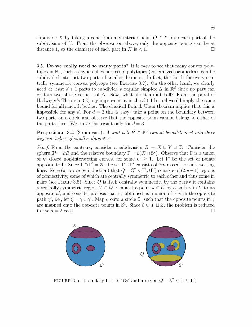
3.5. Do we really need so many parts? It is easy to see that many convex poly-topes in Rd, such as hypercubes and cross-polytopes (generalized octahedra), can besubdivided into just two parts of smaller diameter. In fact, this holds for every cen-trally symmetric convex polytope (see Exercise 3.2). On the other hand, we clearlyneed at least d + 1 parts to subdivide a regular simplex ∆ in Rd since no part cancontain two of the vertices of ∆. Now, what about a unit ball? From the proof ofHadwiger’s Theorem 3.3, any improvement in the d+ 1 bound would imply the samebound for all smooth bodies. The classical Borsuk-Ulam theorem implies that this isimpossible for any d. For d = 2 this is easy: take a point on the boundary betweentwo parts on a circle and observe that the opposite point cannot belong to either ofthe parts then. We prove this result only for d = 3.

Proposition 3.4 (3-dim case). A unit ball B ⊂ R3 cannot be subdivided into threedisjoint bodies of smaller diameter.

Proof. From the contrary, consider a subdivision B = X ⊔ Y ⊔ Z. Consider thesphere S2 = ∂B and the relative boundary Γ = ∂(X ∩ S2). Observe that Γ is a unionof m closed non-intersecting curves, for some m ≥ 1. Let Γ′ be the set of pointsopposite to Γ. Since Γ∩ Γ′ = ∅, the set Γ∪ Γ′ consists of 2m closed non-intersectinglines. Note (or prove by induction) that Q = S2r (Γ∪Γ′) consists of (2m+1) regionsof connectivity, some of which are centrally symmetric to each other and thus come inpairs (see Figure 3.5). Since Q is itself centrally symmetric, by the parity it containsa centrally symmetric region U ⊂ Q. Connect a point u ⊂ U by a path γ in U to itsopposite u′, and consider a closed path ζ obtained as a union of γ with the oppositepath γ′, i.e., let ζ = γ ∪ γ′. Map ζ onto a circle S1 such that the opposite points in ζare mapped onto the opposite points in S1. Since ζ ⊂ Y ⊔ Z, the problem is reducedto the d = 2 case.

X

S2 S2

Q

Figure 3.5. Boundary Γ = X ∩ S2 and a region Q = S2 r (Γ ∪ Γ′).

30

3.6. Exercises.

Exercise 3.1. [1-] Prove that every convex polygon X of area 1 can be covered by arectangle of area 2.

Exercise 3.2. a) [1] Prove that centrally symmetric polytopes in Rd can be subdividedinto two subsets of smaller diameter.b) [1] Prove the Borsuk conjecture for centrally symmetric convex sets X ⊂ Rd.

Exercise 3.3. [1-] Prove that every set of n points in R3 with diameter ℓ, can be coveredby a cube with side length ℓ.

Exercise 3.4. (Pal) a) [1+] Prove that every convex set of unit diameter can be coveredby a hexagon with side 1.b) [1-] Prove that every convex set of unit diameter can be subdivided into three convex

sets of diameter at most√

32 .

c) [2-] Prove that every planar set of n points of unit diameter can be partitioned into three

subsets of diameter less than√

32 cos 2π

3n(n−1) .

Exercise 3.5. (Borsuk conjecture in R3) [2] Prove the Borsuk conjecture for convex setsX ⊂ R3.

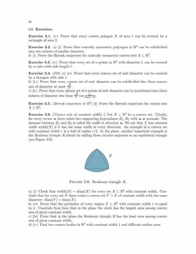
Exercise 3.6. (Convex sets of constant width) ♦ Let X ⊂ Rd be a convex set. Clearly,for every vector u there exists two supporting hyperplanes H1,H2 with u as normals. Thedistance between H1 and H2 is called the width in direction u . We say that X has constantwidth width(X) if it has the same width in every direction. An example of a convex setwith constant width r is a ball of radius r/2. In the plane, another important example isthe Reuleaux triangle R obtain by adding three circular segments to an equilateral triangle(see Figure 3.6).

R

Figure 3.6. Reuleaux triangle R.

a) [1] Check that width(X) = diam(X) for every set X ⊂ Rd with constant width. Con-clude that for every set X there exists a convex set Y ⊃ X of constant width with the samediameter: diam(Y ) = diam(X).b) [1+] Prove that the perimeter of every region X ⊂ R2 with constant width 1 is equalto π. Conclude from here that in the plane the circle has the largest area among convexsets of given constant width.c) [2+] Prove that in the plane the Reuleaux triangle R has the least area among convexsets of given constant width.d) [1-] Find two convex bodies in R3 with constant width 1 and different surface area.

31

Exercise 3.7. [1] Let X ⊂ R2 be a body of constant width. Observe that every rectanglecircumscribed around X is a square (see Subsection 5.1). Prove that the converse result isfalse even if one assumes that X is smooth.

Exercise 3.8. (Covering disks with disks) Denote by Rk the maximum radius of a diskwhich can be covered with k unit disks.a) [1] Prove that R2 = 1, R3 = 2√

3and R4 =

√2.

b) [1] Prove that R5 > 1.64.c) [2-] Find the exact value for R5.d) [1+] Prove that R7 = 2.e) [1+] Prove that R9 = 1 + 2 cos 2π

8 .

Exercise 3.9. A finite set of points A ⊂ R2 is said to be coverable if there is a finitecollection of disjoint unit disks which covers A. Denote by N the size of the smallest set Awhich is not coverable.a) [1] Prove that N < 100.b) [1] Prove that N > 10.

3.7. Final remarks. Recall that our proof of the Borsuk conjecture in dimension 2 isrobust, i.e., produces a subdivision into three parts, such that each of them have diam ≤(1 − ε), for some universal constant ε > 0. Although not phrased that way by Borsuk,we think this relatively small extension makes an important distinction; we emphasize therobustness in the statement of Theorem 3.2. Dimension 3 is the only other dimension inwhich the Borsuk conjecture has been proved, by Eggleston in 1955, and that proof is alsorobust (a simplified proof was published by Grunbaum [BolG]). However, our proof of theHadwiger theorem (Theorem 3.3) is inherently different and in fact cannot be convertedinto a robust proof. We refer to [BMS, §31] for an overview of the subject, various positiveand negative results and references.

The ‘extended meditation’ proof of the Borsuk theorem is due to the author, and is similarto other known proofs. The standard proof uses Pal’s theorem (see Exercise 3.4) that everysuch X can be covered by a regular hexagon with side 1, which gives an optimal bound on ε(see [BolG, HDK]). The proof in the smooth case is a reworked proof given in [BolG, §7].The proof in Proposition 3.4 may seem simple enough, but in essence it coincides with theearly induction step of a general theorem. For this and other applications of the topologicalapproach see [Mat2].

The high-dimensional counterexamples of Kahn–Kalai [KahK] (to the Borsuk conjecture)

come from a family of polytopes spanned by subsets of vertices of a d-dimensional cube,

whose vertices are carefully chosen to have many equal distances. We refer to [AigZ, §15] for

an elegant exposition. In addition, we recommend a videotaped lecture by Gil Kalai [Kal2]

which gives a nice survey of the current state of art with some interesting conjectures and

promising research venues.

32

4. Fair division

In this section we begin our study of topological arguments, which is further con-tinued in the next two sections. Although the results in this section are largelyelementary, they have beautiful applications.

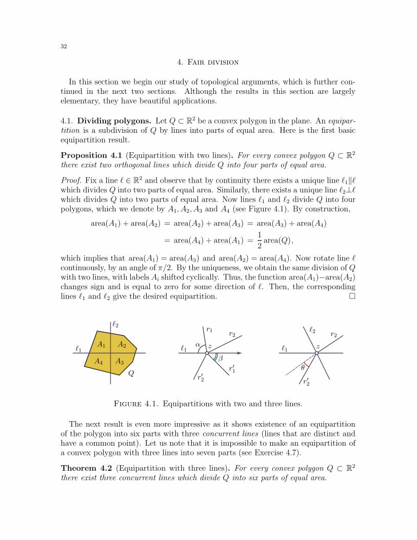
4.1. Dividing polygons. Let Q ⊂ R2 be a convex polygon in the plane. An equipar-tition is a subdivision of Q by lines into parts of equal area. Here is the first basicequipartition result.

Proposition 4.1 (Equipartition with two lines). For every convex polygon Q ⊂ R2

there exist two orthogonal lines which divide Q into four parts of equal area.

Proof. Fix a line ℓ ∈ R2 and observe that by continuity there exists a unique line ℓ1‖ℓwhich divides Q into two parts of equal area. Similarly, there exists a unique line ℓ2⊥ℓwhich divides Q into two parts of equal area. Now lines ℓ1 and ℓ2 divide Q into fourpolygons, which we denote by A1, A2, A3 and A4 (see Figure 4.1). By construction,

area(A1) + area(A2) = area(A2) + area(A3) = area(A3) + area(A4)

= area(A4) + area(A1) =1

2area(Q),

which implies that area(A1) = area(A3) and area(A2) = area(A4). Now rotate line ℓcontinuously, by an angle of π/2. By the uniqueness, we obtain the same division of Qwith two lines, with labels Ai shifted cyclically. Thus, the function area(A1)−area(A2)changes sign and is equal to zero for some direction of ℓ. Then, the correspondinglines ℓ1 and ℓ2 give the desired equipartition.

ℓ1ℓ1ℓ1

ℓ2ℓ2

A1 A2

A3A4

r1 r2r2

r′1

r′2r′2

zz

θβ

α

Q

Figure 4.1. Equipartitions with two and three lines.

The next result is even more impressive as it shows existence of an equipartitionof the polygon into six parts with three concurrent lines (lines that are distinct andhave a common point). Let us note that it is impossible to make an equipartition ofa convex polygon with three lines into seven parts (see Exercise 4.7).

Theorem 4.2 (Equipartition with three lines). For every convex polygon Q ⊂ R2

there exist three concurrent lines which divide Q into six parts of equal area.

33

Proof. Fix a line ℓ ⊂ R2 and take ℓ1‖ℓ which divides Q into two parts of equal area.For every point z ∈ ℓ1 there there is a unique collections of rays r2, r3, r

′2 and r′3 which

start at z and together with ℓ1 divide Q into six parts of equal area (see Figure 4.1).Move z continuously along ℓ1. Observe that the angle α defined as in the figure,decreases from π to 0, while angle β increases from 0 to π. By continuity, there existsa unique point z such that r2 and r′2 form a line. Denote this line by ℓ2. As in theprevious proof, rotate ℓ continuously, by an angle of π. At the end, we obtain thesame partition, with the roles of r3 and r′3 interchanged. Thus, the angle θ betweenlines spanned by r3 and r′3 changes sign and at some point is equal to zero. Rays r3and r′3 then form a line which we denote by ℓ3. Then, lines ℓ1, ℓ2 and ℓ3 gives thedesired equipartition.

4.2. Back to points, lines and triangles. The following result is a special case ofthe Barany theorem (Theorem 2.2), with an explicit constant. We obtain it as easyapplication of the equipartition with three lines (Theorem 4.2).

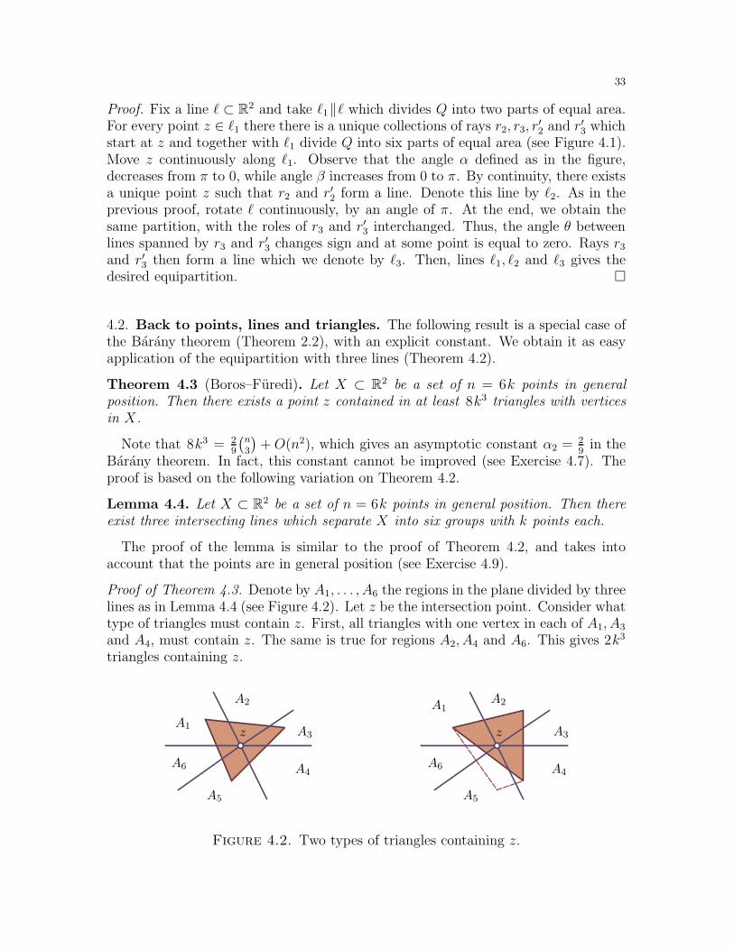
Theorem 4.3 (Boros–Furedi). Let X ⊂ R2 be a set of n = 6k points in generalposition. Then there exists a point z contained in at least 8k3 triangles with verticesin X.

Note that 8k3 = 29

(n3

)+O(n2), which gives an asymptotic constant α2 = 2

9in the

Barany theorem. In fact, this constant cannot be improved (see Exercise 4.7). Theproof is based on the following variation on Theorem 4.2.

Lemma 4.4. Let X ⊂ R2 be a set of n = 6k points in general position. Then thereexist three intersecting lines which separate X into six groups with k points each.

The proof of the lemma is similar to the proof of Theorem 4.2, and takes intoaccount that the points are in general position (see Exercise 4.9).

Proof of Theorem 4.3. Denote by A1, . . . , A6 the regions in the plane divided by threelines as in Lemma 4.4 (see Figure 4.2). Let z be the intersection point. Consider whattype of triangles must contain z. First, all triangles with one vertex in each of A1, A3

and A4, must contain z. The same is true for regions A2, A4 and A6. This gives 2k3

triangles containing z.

A1

A1

A2A2

A3A3

A4A4

A5A5

A6A6

zz

Figure 4.2. Two types of triangles containing z.

34

Similarly, for every two vertices in the opposite regions A1 and A4 there exist atleast 2k ways to form a triangle which contains z, with either all vertices in A2 ∪A3

or with all vertices in A4 ∪ A5 (see Figure 4.2). This gives at least 2k3 trianglescontaining z. Since the same argument holds for the other two pairs of oppositeregions, we get at least 6k3 triangles of this type, and 8k3 in total.

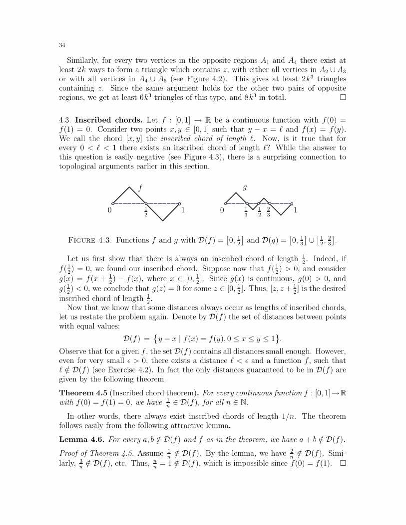
4.3. Inscribed chords. Let f : [0, 1] → R be a continuous function with f(0) =f(1) = 0. Consider two points x, y ∈ [0, 1] such that y − x = ℓ and f(x) = f(y).We call the chord [x, y] the inscribed chord of length ℓ. Now, is it true that forevery 0 < ℓ < 1 there exists an inscribed chord of length ℓ? While the answer tothis question is easily negative (see Figure 4.3), there is a surprising connection totopological arguments earlier in this section.

f g

11 00 12

12

13

23

Figure 4.3. Functions f and g with D(f) =[0, 1

2

]and D(g) =

[0, 1

3

]∪[

12, 2

3

].

Let us first show that there is always an inscribed chord of length 12. Indeed, if

f(12) = 0, we found our inscribed chord. Suppose now that f(1

2) > 0, and consider

g(x) = f(x + 12) − f(x), where x ∈ [0, 1

2]. Since g(x) is continuous, g(0) > 0, and

g(12) < 0, we conclude that g(z) = 0 for some z ∈ [0, 1

2]. Thus, [z, z+ 1

2] is the desired

inscribed chord of length 12.

Now that we know that some distances always occur as lengths of inscribed chords,let us restate the problem again. Denote by D(f) the set of distances between pointswith equal values:

D(f) =y − x | f(x) = f(y), 0 ≤ x ≤ y ≤ 1

.

Observe that for a given f , the set D(f) contains all distances small enough. However,even for very small ǫ > 0, there exists a distance ℓ < ǫ and a function f , such thatℓ /∈ D(f) (see Exercise 4.2). In fact the only distances guaranteed to be in D(f) aregiven by the following theorem.

Theorem 4.5 (Inscribed chord theorem). For every continuous function f : [0, 1]→Rwith f(0) = f(1) = 0, we have 1

n∈ D(f), for all n ∈ N.

In other words, there always exist inscribed chords of length 1/n. The theoremfollows easily from the following attractive lemma.

Lemma 4.6. For every a, b /∈ D(f) and f as in the theorem, we have a+ b /∈ D(f).

Proof of Theorem 4.5. Assume 1n/∈ D(f). By the lemma, we have 2

n/∈ D(f). Simi-

larly, 3n/∈ D(f), etc. Thus, n

n= 1 /∈ D(f), which is impossible since f(0) = f(1).

35

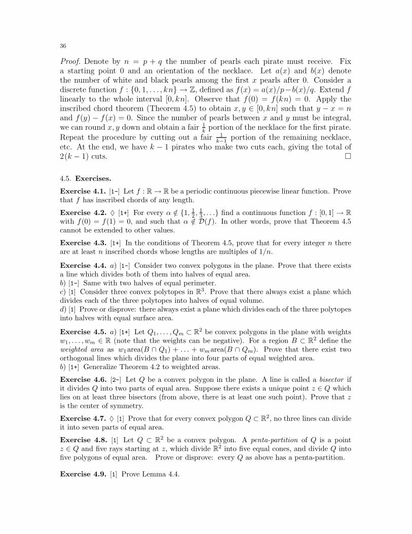
Proof of Lemma 4.6. Denote by G the graph of function f , and by Gℓ the graph Gshifted by ℓ, where ℓ ∈ R. Attach toG two vertical rays: at the first (global) maximumof f pointing up and at the first (global) minimum pointing down (see Figure 4.4).Do the same with Gℓ. Now observe that ℓ ∈ D(f) is equivalent to having G and Gℓ

intersect. Since a, b /∈ D(f), then graph G does not intersect graphs G−a and Gb. Byconstruction, graph G divides the plane into two parts. We conclude that graphs G−aand Gb lie in different parts, and thus do not intersect. By the symmetry, this impliesthat G and Ga+b do not intersect, and therefore a+ b /∈ D(f).

0 001

11

G GG

Gℓ′

ℓ′ ℓ′ + 1

Gℓ

ℓ

ℓ

ℓ

ℓ+ 1

Figure 4.4. Graphs G, Gℓ and Gℓ′, where ℓ ∈ D(f) and G ∩Gℓ 6= ∅,while ℓ′ /∈ D(f) and G ∩Gℓ′ = ∅.

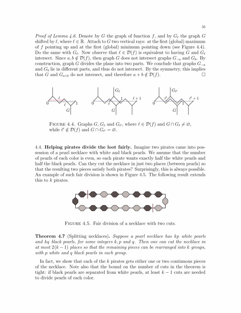
4.4. Helping pirates divide the loot fairly. Imagine two pirates came into pos-session of a pearl necklace with white and black pearls. We assume that the numberof pearls of each color is even, so each pirate wants exactly half the white pearls andhalf the black pearls. Can they cut the necklace in just two places (between pearls) sothat the resulting two pieces satisfy both pirates? Surprisingly, this is always possible.An example of such fair division is shown in Figure 4.5. The following result extendsthis to k pirates.

Figure 4.5. Fair division of a necklace with two cuts.

Theorem 4.7 (Splitting necklaces). Suppose a pearl necklace has kp white pearlsand kq black pearls, for some integers k, p and q. Then one can cut the necklace inat most 2(k− 1) places so that the remaining pieces can be rearranged into k groups,with p white and q black pearls in each group.

In fact, we show that each of the k pirates gets either one or two continuous piecesof the necklace. Note also that the bound on the number of cuts in the theorem istight: if black pearls are separated from white pearls, at least k − 1 cuts are neededto divide pearls of each color.

36

Proof. Denote by n = p + q the number of pearls each pirate must receive. Fixa starting point 0 and an orientation of the necklace. Let a(x) and b(x) denotethe number of white and black pearls among the first x pearls after 0. Consider adiscrete function f : 0, 1, . . . , kn → Z, defined as f(x) = a(x)/p−b(x)/q. Extend flinearly to the whole interval [0, kn]. Observe that f(0) = f(kn) = 0. Apply theinscribed chord theorem (Theorem 4.5) to obtain x, y ∈ [0, kn] such that y − x = nand f(y)− f(x) = 0. Since the number of pearls between x and y must be integral,we can round x, y down and obtain a fair 1

kportion of the necklace for the first pirate.

Repeat the procedure by cutting out a fair 1k−1

portion of the remaining necklace,etc. At the end, we have k − 1 pirates who make two cuts each, giving the total of2(k − 1) cuts.

4.5. Exercises.

Exercise 4.1. [1-] Let f : R→ R be a periodic continuous piecewise linear function. Provethat f has inscribed chords of any length.

Exercise 4.2. ♦ [1+] For every α /∈ 1, 12 ,

13 , . . . find a continuous function f : [0, 1] → R

with f(0) = f(1) = 0, and such that α /∈ D(f). In other words, prove that Theorem 4.5cannot be extended to other values.

Exercise 4.3. [1+] In the conditions of Theorem 4.5, prove that for every integer n thereare at least n inscribed chords whose lengths are multiples of 1/n.

Exercise 4.4. a) [1-] Consider two convex polygons in the plane. Prove that there existsa line which divides both of them into halves of equal area.b) [1-] Same with two halves of equal perimeter.c) [1] Consider three convex polytopes in R3. Prove that there always exist a plane whichdivides each of the three polytopes into halves of equal volume.d) [1] Prove or disprove: there always exist a plane which divides each of the three polytopesinto halves with equal surface area.

Exercise 4.5. a) [1+] Let Q1, . . . , Qm ⊂ R2 be convex polygons in the plane with weightsw1, . . . , wm ∈ R (note that the weights can be negative). For a region B ⊂ R2 define theweighted area as w1area(B ∩ Q1) + . . . + wmarea(B ∩ Qm). Prove that there exist twoorthogonal lines which divides the plane into four parts of equal weighted area.b) [1+] Generalize Theorem 4.2 to weighted areas.

Exercise 4.6. [2-] Let Q be a convex polygon in the plane. A line is called a bisector ifit divides Q into two parts of equal area. Suppose there exists a unique point z ∈ Q whichlies on at least three bisectors (from above, there is at least one such point). Prove that zis the center of symmetry.

Exercise 4.7. ♦ [1] Prove that for every convex polygon Q ⊂ R2, no three lines can divideit into seven parts of equal area.

Exercise 4.8. [1] Let Q ⊂ R2 be a convex polygon. A penta-partition of Q is a pointz ∈ Q and five rays starting at z, which divide R2 into five equal cones, and divide Q intofive polygons of equal area. Prove or disprove: every Q as above has a penta-partition.

Exercise 4.9. [1] Prove Lemma 4.4.

37

Exercise 4.10. ♦ [1+] Give an example showing that the α2 = 29 in Barany’s theorem is

optimal (see Theorem 2.2 and Theorem 4.3).

Exercise 4.11. [2] Let Q ⊂ R2 be a convex polygon in the plane. Prove that there existsa convex quadrilateral X = [x1x2x3x4] such that X together with lines (x1x3) and (x2x4)divide Q into eight regions of equal area (see Figure 4.6).10 Generalize this to polygons Qiand weighted area (see Exercise 4.5).

Q

x1

x2

x3

x4

Figure 4.6. Cutting a polygon into eight regions of equal area.

Exercise 4.12. [2-] Let P ⊂ R3 be a convex polytope. Prove that there exist threeorthogonal planes, such that every two of them divide P into four parts of equal volume.

Exercise 4.13. a) [1+] Suppose a necklace has 2p white, 2q black, and 2r red pearls. Provethat three cuts suffice to divide the necklace fairly between two pirates.b) [1-] Check that two cuts may not be enough.c) [2] Prove that for k pirates and s ≥ 2 types of pearls, s(k − 1) cuts always suffice.

Exercise 4.14. [1] Two pirates found a necklace with pearls of n different sizes, and eachsize comes in two colors: black and white. They observed that the sizes of white pearlsincrease clockwise, while the size of black pearls increase counterclockwise. Pirates wantto divide the necklace so that each gets a pearl of every size. Prove that two cuts alwayssuffice.

Exercise 4.15. (Two integrals theorem) Let f, g : [0, 1] → [0, 1] be two continuous func-

tions such that∫ 10 f =

∫ 10 g = 1.

a) [1] Prove that there exist 0 ≤ α < β ≤ 1, such that∫ βα f =

∫ βα g = 1/2.

b) [1+] Suppose for some 0 < a < 1 and every 0 ≤ α < β ≤ 1, either∫ βα f 6= a or

∫ βα g 6= a.

Prove that there exist 0 ≤ α < β ≤ 1, such that∫ βα f =

∫ βα g = 1− a.

c) [1] Prove that for every n ∈ N, there exist 0 ≤ α < β ≤ 1, such that∫ βα f =

∫ βα g = 1/n.

4.6. Final remarks. The equipartition with two lines goes back to [CouR, §6.6]. Theo-rem 4.2 is proved in [Buck] (see also Exercises 4.5 and 4.7). For the background, general-izations and references on classical equipartition results see [Gru2, §4.2].

10This is called cobweb equipartition.

38

The Boros–Furedi theorem is proved in [BorF]. Our proof follows a recent paper [Bukh].For a matching lower bound, the original proof has been shown to be false, and a completeproof is given in [BMN] (see Exercise 4.10).

The inscribed chord theorem (Theorem 4.5) is usually attributed to Levy (1934). It waspointed out in [Fle] that the result was first discovered by Ampere in 1806. The proof wepresent is due to Hopf [Hop1]. Our presentation follows [Lyu, §34].

Theorem 4.7 is due to Goldberg and West (1985), and was further generalized a number

of times. Notably, Alon showed in [Alon] that for k pirates and s ≥ 2 types of pearls,

s(k − 1) cuts suffice (see Exercise 4.13). We refer to [Mat2, §3.2, §6.6] for further results,

proofs and references. Our presentation is a variation on several known proofs and was

partly influenced by [Tot].

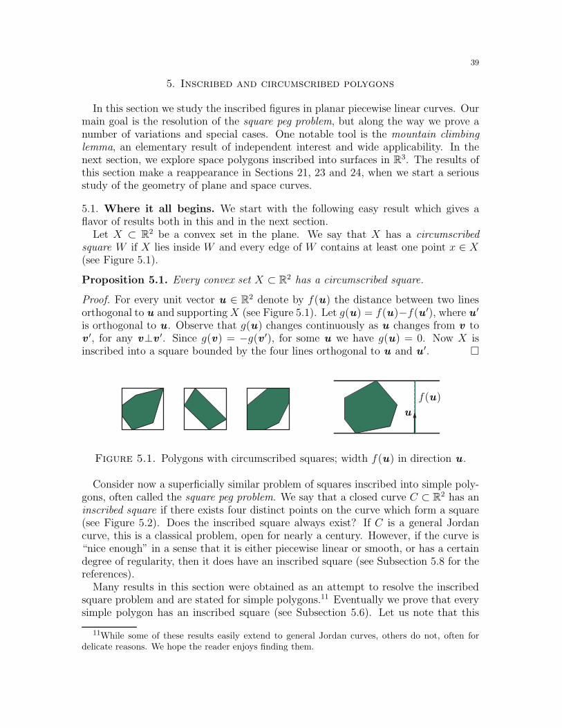
39

5. Inscribed and circumscribed polygons

In this section we study the inscribed figures in planar piecewise linear curves. Ourmain goal is the resolution of the square peg problem, but along the way we prove anumber of variations and special cases. One notable tool is the mountain climbinglemma, an elementary result of independent interest and wide applicability. In thenext section, we explore space polygons inscribed into surfaces in R3. The results ofthis section make a reappearance in Sections 21, 23 and 24, when we start a seriousstudy of the geometry of plane and space curves.

5.1. Where it all begins. We start with the following easy result which gives aflavor of results both in this and in the next section.

Let X ⊂ R2 be a convex set in the plane. We say that X has a circumscribedsquare W if X lies inside W and every edge of W contains at least one point x ∈ X(see Figure 5.1).

Proposition 5.1. Every convex set X ⊂ R2 has a circumscribed square.

Proof. For every unit vector u ∈ R2 denote by f(u) the distance between two linesorthogonal to u and supportingX (see Figure 5.1). Let g(u) = f(u)−f(u ′), where u

′

is orthogonal to u . Observe that g(u) changes continuously as u changes from v tov′, for any v⊥v

′. Since g(v) = −g(v ′), for some u we have g(u) = 0. Now X isinscribed into a square bounded by the four lines orthogonal to u and u

′.

f(u)

u

Figure 5.1. Polygons with circumscribed squares; width f(u) in direction u .

Consider now a superficially similar problem of squares inscribed into simple poly-gons, often called the square peg problem. We say that a closed curve C ⊂ R2 has aninscribed square if there exists four distinct points on the curve which form a square(see Figure 5.2). Does the inscribed square always exist? If C is a general Jordancurve, this is a classical problem, open for nearly a century. However, if the curve is“nice enough” in a sense that it is either piecewise linear or smooth, or has a certaindegree of regularity, then it does have an inscribed square (see Subsection 5.8 for thereferences).

Many results in this section were obtained as an attempt to resolve the inscribedsquare problem and are stated for simple polygons.11 Eventually we prove that everysimple polygon has an inscribed square (see Subsection 5.6). Let us note that this

11While some of these results easily extend to general Jordan curves, others do not, often fordelicate reasons. We hope the reader enjoys finding them.

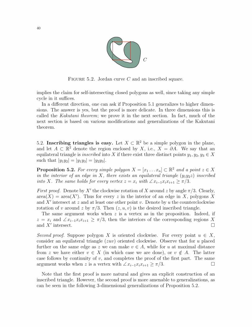
40

C

Figure 5.2. Jordan curve C and an inscribed square.

implies the claim for self-intersecting closed polygons as well, since taking any simplecycle in it suffices.

In a different direction, one can ask if Proposition 5.1 generalizes to higher dimen-sions. The answer is yes, but the proof is more delicate. In three dimensions this iscalled the Kakutani theorem; we prove it in the next section. In fact, much of thenext section is based on various modifications and generalizations of the Kakutanitheorem.

5.2. Inscribing triangles is easy. Let X ⊂ R2 be a simple polygon in the plane,and let A ⊂ R2 denote the region enclosed by X, i.e., X = ∂A. We say that anequilateral triangle is inscribed into X if there exist three distinct points y1, y2, y3 ∈ Xsuch that |y1y2| = |y1y3| = |y2y3|.

Proposition 5.2. For every simple polygon X = [x1 . . . xn] ⊂ R2 and a point z ∈ Xin the interior of an edge in X, there exists an equilateral triangle (y1y2z) inscribedinto X. The same holds for every vertex z = xi with ∠xi−1xixi+1 ≥ π/3.

First proof. Denote by X ′ the clockwise rotation ofX around z by angle π/3. Clearly,area(X) = area(X ′). Thus for every z in the interior of an edge in X, polygons Xand X ′ intersect at z and at least one other point v. Denote by u the counterclockwiserotation of v around z by π/3. Then (z, u, v) is the desired inscribed triangle.

The same argument works when z is a vertex as in the proposition. Indeed, ifz = xi and ∠xi−1xixi+1 ≥ π/3, then the interiors of the corresponding regions Xand X ′ intersect.

Second proof. Suppose polygon X is oriented clockwise. For every point u ∈ X,consider an equilateral triangle (zuv) oriented clockwise. Observe that for u placedfurther on the same edge as z we can make v ∈ A, while for u at maximal distancefrom z we have either v ∈ X (in which case we are done), or v /∈ A. The lattercase follows by continuity of v, and completes the proof of the first part. The sameargument works when z is a vertex with ∠xi−1xixi+1 ≥ π/3.

Note that the first proof is more natural and gives an explicit construction of aninscribed triangle. However, the second proof is more amenable to generalizations, ascan be seen in the following 3-dimensional generalizations of Proposition 5.2.

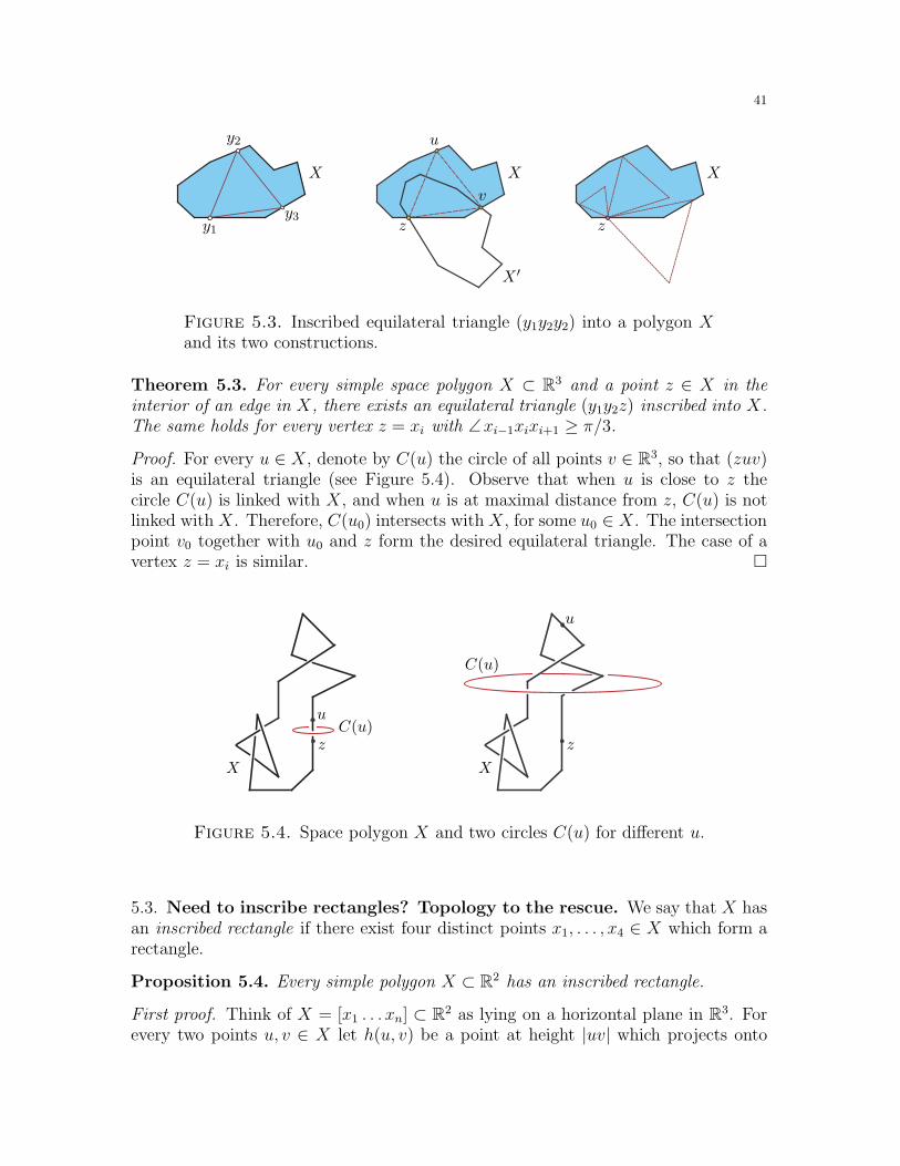
41

y1

y2

y3

XX X

X ′

zz

u

v

Figure 5.3. Inscribed equilateral triangle (y1y2y2) into a polygon Xand its two constructions.

Theorem 5.3. For every simple space polygon X ⊂ R3 and a point z ∈ X in theinterior of an edge in X, there exists an equilateral triangle (y1y2z) inscribed into X.The same holds for every vertex z = xi with ∠xi−1xixi+1 ≥ π/3.

Proof. For every u ∈ X, denote by C(u) the circle of all points v ∈ R3, so that (zuv)is an equilateral triangle (see Figure 5.4). Observe that when u is close to z thecircle C(u) is linked with X, and when u is at maximal distance from z, C(u) is notlinked with X. Therefore, C(u0) intersects with X, for some u0 ∈ X. The intersectionpoint v0 together with u0 and z form the desired equilateral triangle. The case of avertex z = xi is similar.

XX

zz

u

u

C(u)

C(u)

Figure 5.4. Space polygon X and two circles C(u) for different u.

5.3. Need to inscribe rectangles? Topology to the rescue. We say that X hasan inscribed rectangle if there exist four distinct points x1, . . . , x4 ∈ X which form arectangle.

Proposition 5.4. Every simple polygon X ⊂ R2 has an inscribed rectangle.

First proof. Think of X = [x1 . . . xn] ⊂ R2 as lying on a horizontal plane in R3. Forevery two points u, v ∈ X let h(u, v) be a point at height |uv| which projects onto

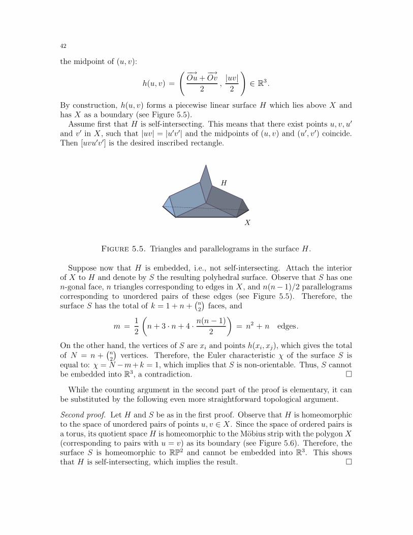
42

the midpoint of (u, v):

h(u, v) =

( −→Ou+

−→Ov

2,|uv|2

)∈ R3 .

By construction, h(u, v) forms a piecewise linear surface H which lies above X andhas X as a boundary (see Figure 5.5).

Assume first that H is self-intersecting. This means that there exist points u, v, u′

and v′ in X, such that |uv| = |u′v′| and the midpoints of (u, v) and (u′, v′) coincide.Then [uvu′v′] is the desired inscribed rectangle.

H

X

Figure 5.5. Triangles and parallelograms in the surface H .

Suppose now that H is embedded, i.e., not self-intersecting. Attach the interiorof X to H and denote by S the resulting polyhedral surface. Observe that S has onen-gonal face, n triangles corresponding to edges in X, and n(n− 1)/2 parallelogramscorresponding to unordered pairs of these edges (see Figure 5.5). Therefore, thesurface S has the total of k = 1 + n +

(n2

)faces, and

m =1

2

(n + 3 · n + 4 · n(n− 1)

2

)= n2 + n edges.

On the other hand, the vertices of S are xi and points h(xi, xj), which gives the totalof N = n +

(n2

)vertices. Therefore, the Euler characteristic χ of the surface S is

equal to: χ = N −m+k = 1, which implies that S is non-orientable. Thus, S cannotbe embedded into R3, a contradiction.

While the counting argument in the second part of the proof is elementary, it canbe substituted by the following even more straightforward topological argument.

Second proof. Let H and S be as in the first proof. Observe that H is homeomorphicto the space of unordered pairs of points u, v ∈ X. Since the space of ordered pairs isa torus, its quotient space H is homeomorphic to the Mobius strip with the polygon X(corresponding to pairs with u = v) as its boundary (see Figure 5.6). Therefore, thesurface S is homeomorphic to RP2 and cannot be embedded into R3. This showsthat H is self-intersecting, which implies the result.

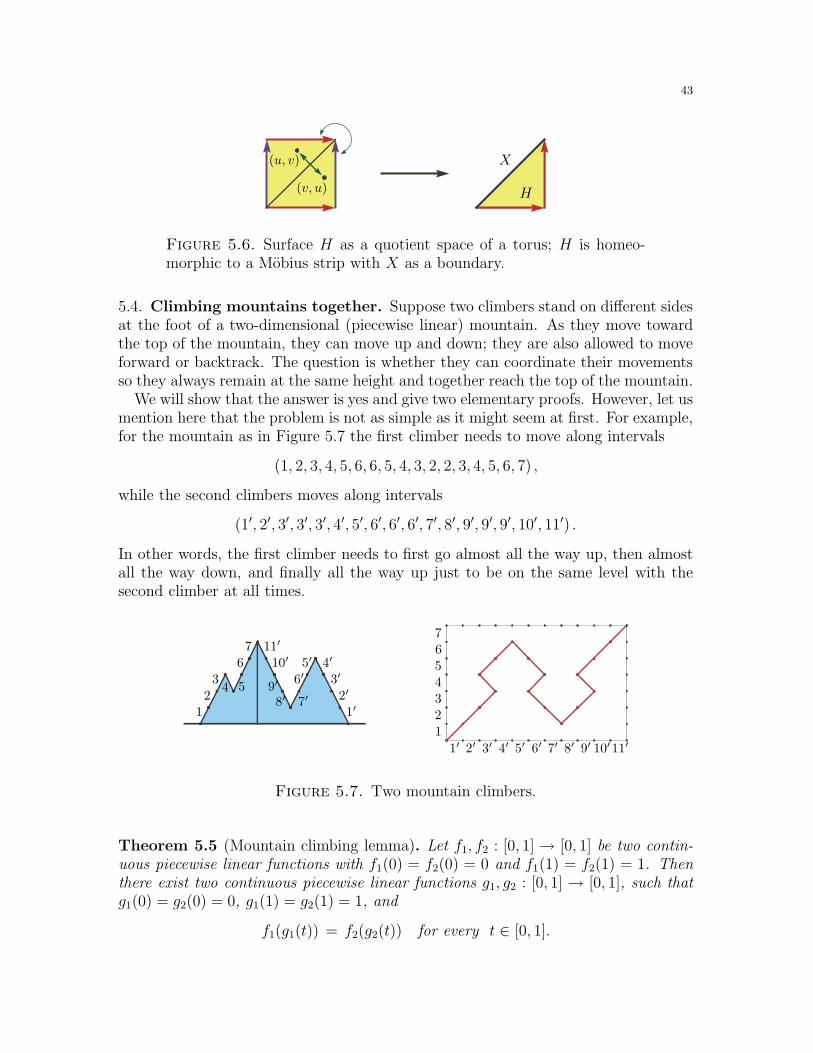
43

(u, v)

(v, u) H

X

Figure 5.6. Surface H as a quotient space of a torus; H is homeo-morphic to a Mobius strip with X as a boundary.

5.4. Climbing mountains together. Suppose two climbers stand on different sidesat the foot of a two-dimensional (piecewise linear) mountain. As they move towardthe top of the mountain, they can move up and down; they are also allowed to moveforward or backtrack. The question is whether they can coordinate their movementsso they always remain at the same height and together reach the top of the mountain.

We will show that the answer is yes and give two elementary proofs. However, let usmention here that the problem is not as simple as it might seem at first. For example,for the mountain as in Figure 5.7 the first climber needs to move along intervals

(1, 2, 3, 4, 5, 6, 6, 5, 4, 3, 2, 2, 3, 4, 5, 6, 7) ,

while the second climbers moves along intervals

(1′, 2′, 3′, 3′, 3′, 4′, 5′, 6′, 6′, 6′, 7′, 8′, 9′, 9′, 9′, 10′, 11′) .

In other words, the first climber needs to first go almost all the way up, then almostall the way down, and finally all the way up just to be on the same level with thesecond climber at all times.

1

1

2

2

3

34 45

56677

1′

1′

2′

2′

3′

3′

4′

4′

5′

5′

6′

6′

7′

7′

8′

8′

9′

9′

10′

10′

11′

11′

Figure 5.7. Two mountain climbers.

Theorem 5.5 (Mountain climbing lemma). Let f1, f2 : [0, 1]→ [0, 1] be two contin-uous piecewise linear functions with f1(0) = f2(0) = 0 and f1(1) = f2(1) = 1. Thenthere exist two continuous piecewise linear functions g1, g2 : [0, 1] → [0, 1], such thatg1(0) = g2(0) = 0, g1(1) = g2(1) = 1, and

f1(g1(t)) = f2(g2(t)) for every t ∈ [0, 1].

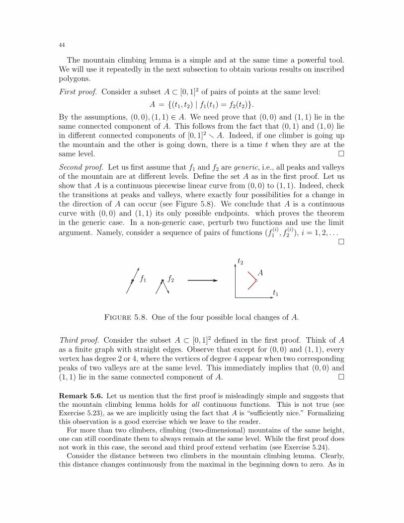
44

The mountain climbing lemma is a simple and at the same time a powerful tool.We will use it repeatedly in the next subsection to obtain various results on inscribedpolygons.

First proof. Consider a subset A ⊂ [0, 1]2 of pairs of points at the same level:

A = (t1, t2) | f1(t1) = f2(t2).By the assumptions, (0, 0), (1, 1) ∈ A. We need prove that (0, 0) and (1, 1) lie in thesame connected component of A. This follows from the fact that (0, 1) and (1, 0) liein different connected components of [0, 1]2 r A. Indeed, if one climber is going upthe mountain and the other is going down, there is a time t when they are at thesame level.

Second proof. Let us first assume that f1 and f2 are generic, i.e., all peaks and valleysof the mountain are at different levels. Define the set A as in the first proof. Let usshow that A is a continuous piecewise linear curve from (0, 0) to (1, 1). Indeed, checkthe transitions at peaks and valleys, where exactly four possibilities for a change inthe direction of A can occur (see Figure 5.8). We conclude that A is a continuouscurve with (0, 0) and (1, 1) its only possible endpoints. which proves the theoremin the generic case. In a non-generic case, perturb two functions and use the limit

argument. Namely, consider a sequence of pairs of functions (f(i)1 , f

(i)2 ), i = 1, 2, . . .

f1 f2

t2

t1

A

Figure 5.8. One of the four possible local changes of A.

Third proof. Consider the subset A ⊂ [0, 1]2 defined in the first proof. Think of Aas a finite graph with straight edges. Observe that except for (0, 0) and (1, 1), everyvertex has degree 2 or 4, where the vertices of degree 4 appear when two correspondingpeaks of two valleys are at the same level. This immediately implies that (0, 0) and(1, 1) lie in the same connected component of A.

Remark 5.6. Let us mention that the first proof is misleadingly simple and suggests thatthe mountain climbing lemma holds for all continuous functions. This is not true (seeExercise 5.23), as we are implicitly using the fact that A is “sufficiently nice.” Formalizingthis observation is a good exercise which we leave to the reader.

For more than two climbers, climbing (two-dimensional) mountains of the same height,one can still coordinate them to always remain at the same level. While the first proof doesnot work in this case, the second and third proof extend verbatim (see Exercise 5.24).

Consider the distance between two climbers in the mountain climbing lemma. Clearly,this distance changes continuously from the maximal in the beginning down to zero. As in

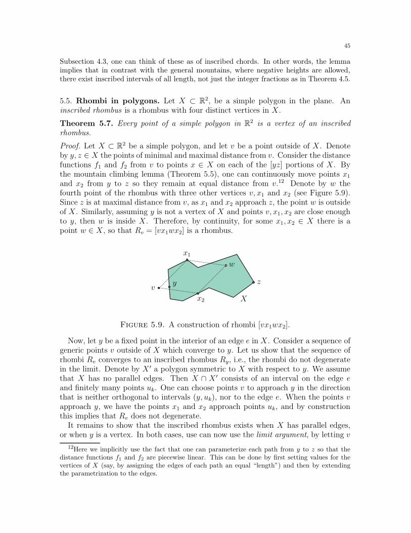
45

Subsection 4.3, one can think of these as of inscribed chords. In other words, the lemmaimplies that in contrast with the general mountains, where negative heights are allowed,there exist inscribed intervals of all length, not just the integer fractions as in Theorem 4.5.

5.5. Rhombi in polygons. Let X ⊂ R2, be a simple polygon in the plane. Aninscribed rhombus is a rhombus with four distinct vertices in X.

Theorem 5.7. Every point of a simple polygon in R2 is a vertex of an inscribedrhombus.

Proof. Let X ⊂ R2 be a simple polygon, and let v be a point outside of X. Denoteby y, z ∈ X the points of minimal and maximal distance from v. Consider the distancefunctions f1 and f2 from v to points x ∈ X on each of the [yz] portions of X. Bythe mountain climbing lemma (Theorem 5.5), one can continuously move points x1

and x2 from y to z so they remain at equal distance from v.12 Denote by w thefourth point of the rhombus with three other vertices v, x1 and x2 (see Figure 5.9).Since z is at maximal distance from v, as x1 and x2 approach z, the point w is outsideof X. Similarly, assuming y is not a vertex of X and points v, x1, x2 are close enoughto y, then w is inside X. Therefore, by continuity, for some x1, x2 ∈ X there is apoint w ∈ X, so that Rv = [vx1wx2] is a rhombus.

x1

x2

v

w

z

X

y

Figure 5.9. A construction of rhombi [vx1wx2].

Now, let y be a fixed point in the interior of an edge e in X. Consider a sequence ofgeneric points v outside of X which converge to y. Let us show that the sequence ofrhombi Rv converges to an inscribed rhombus Ry, i.e., the rhombi do not degeneratein the limit. Denote by X ′ a polygon symmetric to X with respect to y. We assumethat X has no parallel edges. Then X ∩ X ′ consists of an interval on the edge eand finitely many points uk. One can choose points v to approach y in the directionthat is neither orthogonal to intervals (y, uk), nor to the edge e. When the points vapproach y, we have the points x1 and x2 approach points uk, and by constructionthis implies that Rv does not degenerate.

It remains to show that the inscribed rhombus exists when X has parallel edges,or when y is a vertex. In both cases, use can now use the limit argument, by letting v

12Here we implicitly use the fact that one can parameterize each path from y to z so that thedistance functions f1 and f2 are piecewise linear. This can be done by first setting values for thevertices of X (say, by assigning the edges of each path an equal “length”) and then by extendingthe parametrization to the edges.

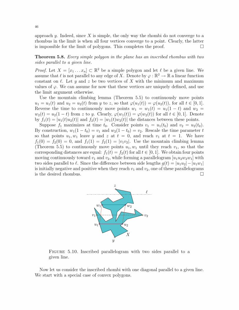
46

approach y. Indeed, since X is simple, the only way the rhombi do not converge to arhombus in the limit is when all four vertices converge to a point. Clearly, the latteris impossible for the limit of polygons. This completes the proof.

Theorem 5.8. Every simple polygon in the plane has an inscribed rhombus with twosides parallel to a given line.

Proof. Let X = [x1 . . . xn] ⊂ R2 be a simple polygon and let ℓ be a given line. Weassume that ℓ is not parallel to any edge ofX. Denote by ϕ : R2 → R a linear functionconstant on ℓ. Let y and z be two vertices of X with the minimum and maximumvalues of ϕ. We can assume for now that these vertices are uniquely defined, and usethe limit argument otherwise.

Use the mountain climbing lemma (Theorem 5.5) to continuously move pointsu1 = u1(t) and u2 = u2(t) from y to z, so that ϕ(u1(t)) = ϕ(u2(t)), for all t ∈ [0, 1].Reverse the time to continuously move points w1 = w1(t) = u1(1 − t) and w2 =w2(t) = u2(1− t) from z to y. Clearly, ϕ(w1(t)) = ϕ(w2(t)) for all t ∈ [0, 1]. Denoteby f1(t) = |u1(t)u2(t)| and f2(t) = |w1(t)w2(t)| the distances between these points.

Suppose f1 maximizes at time t0. Consider points v1 = u1(t0) and v2 = u2(t0).By construction, w1(1− t0) = v1 and w2(1− t0) = v2. Rescale the time parameter tso that points u1, w1 leave y and z at t = 0, and reach v1 at t = 1. We havef1(0) = f2(0) = 0, and f1(1) = f2(1) = |v1v2|. Use the mountain climbing lemma(Theorem 5.5) to continuously move points u1, w1 until they reach v1, so that thecorresponding distances are equal: f1(t) = f2(t) for all t ∈ [0, 1]. We obtain four pointsmoving continuously toward v1 and v2, while forming a parallelogram [u1u2w2w1] withtwo sides parallel to ℓ. Since the difference between side lengths g(t) = |u1u2|−|u1w1|is initially negative and positive when they reach v1 and v2, one of these parallelogramsis the desired rhombus.

y

z

v1 v2

u1 u2

w1 w2

ℓ

X

Figure 5.10. Inscribed parallelogram with two sides parallel to agiven line.

Now let us consider the inscribed rhombi with one diagonal parallel to a given line.We start with a special case of convex polygons.

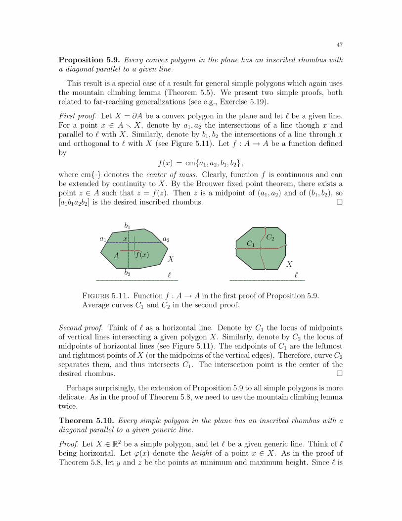
47

Proposition 5.9. Every convex polygon in the plane has an inscribed rhombus witha diagonal parallel to a given line.

This result is a special case of a result for general simple polygons which again usesthe mountain climbing lemma (Theorem 5.5). We present two simple proofs, bothrelated to far-reaching generalizations (see e.g., Exercise 5.19).

First proof. Let X = ∂A be a convex polygon in the plane and let ℓ be a given line.For a point x ∈ A r X, denote by a1, a2 the intersections of a line though x andparallel to ℓ with X. Similarly, denote by b1, b2 the intersections of a line through xand orthogonal to ℓ with X (see Figure 5.11). Let f : A → A be a function definedby

f(x) = cma1, a2, b1, b2,where cm· denotes the center of mass. Clearly, function f is continuous and canbe extended by continuity to X. By the Brouwer fixed point theorem, there exists apoint z ∈ A such that z = f(z). Then z is a midpoint of (a1, a2) and of (b1, b2), so[a1b1a2b2] is the desired inscribed rhombus.

a1 a2

b1

b2

x

A XX

f(x)

ℓ ℓ

C1

C2

Figure 5.11. Function f : A→ A in the first proof of Proposition 5.9.Average curves C1 and C2 in the second proof.

Second proof. Think of ℓ as a horizontal line. Denote by C1 the locus of midpointsof vertical lines intersecting a given polygon X. Similarly, denote by C2 the locus ofmidpoints of horizontal lines (see Figure 5.11). The endpoints of C1 are the leftmostand rightmost points ofX (or the midpoints of the vertical edges). Therefore, curve C2

separates them, and thus intersects C1. The intersection point is the center of thedesired rhombus.

Perhaps surprisingly, the extension of Proposition 5.9 to all simple polygons is moredelicate. As in the proof of Theorem 5.8, we need to use the mountain climbing lemmatwice.

Theorem 5.10. Every simple polygon in the plane has an inscribed rhombus with adiagonal parallel to a given generic line.

Proof. Let X ∈ R2 be a simple polygon, and let ℓ be a given generic line. Think of ℓbeing horizontal. Let ϕ(x) denote the height of a point x ∈ X. As in the proof ofTheorem 5.8, let y and z be the points at minimum and maximum height. Since ℓ is

48

generic, these points are unique. Without loss of generality, we assume that ϕ(y) = 0and ϕ(z) = 1.

Use the mountain climbing lemma (Theorem 5.5) to continuously and piecewiselinearly (in time t) move points u1 = u1(t) and u2 = u2(t) from y to z, so that theyremain at the same height, for all t ∈ [0, 1] (see Figure 5.12). We will show that(u1(t), u2(t)) is a diagonal of a rhombus, for some t ∈ [0, 1]. Let us remark here thatnot all pairs of points at the same height may necessarily appear as (u1, u2).

ℓ

u1 u2

y

z

v

w

L X ′

X ′′

Figure 5.12. Line L⊥ℓ through midpoints of an interval (u1, u2) ‖ ℓ.

For every t ∈ [0, 1], consider a vertical line L through the midpoints of (u1(t), u2(t))and plot the height h = ϕ(x) of the intersection points x ∈ L ∩X in a graph

Γ = (t, h), 0 ≤ t ≤ 1.By construction, the resulting graph Γ is a union of non-intersecting piecewise linearcurves. There are at least two curve endpoints at t = 0 and at least two curveendpoints at t = 1. We will prove that there are at least two continuous curves in Γwith one endpoint at t = 0 and one at t = 1 (see Figure 5.13).

Denote by v and w the leftmost and the rightmost points in X (see Figure 5.11).They separate the polygon into two curves X ′ and X ′′. Since the intersection pointsalways lie between these, there is always an odd number of intersection points withX ′.Therefore, there exists a continuous curve in Γ with one endpoint in X ′ at t = 0 andone endpoint in X ′ at t = 1. The same is true for X ′′, which proves the claim.Denote these curves by C ′ and C ′′, respectively. In general, curves C ′ and C ′′ are notfunctions of t. Use the mountain climbing lemma to parameterize the curves

C ′ = (h1(τ), t1(τ)

), τ ∈ [0, 1] and C ′′ = (h2(τ), t2(τ)

), τ ∈ [0, 1],

so that t1(τ) = t2(τ). Now define the average curve C∗ of C ′ and C ′′ as

C∗ =(h1(τ)/2 + h2(τ)/2, t1(τ)

), τ ∈ [0, 1]

.

By construction, curve C∗ is continuous, starts at t = 0 and ends at t = 1.Consider a curve H given by the function h(t) = ϕ(u1(t)). Plot H and the average

curve C∗ on the same graph as in Figure 5.13. Since h(t) is a continuous function,

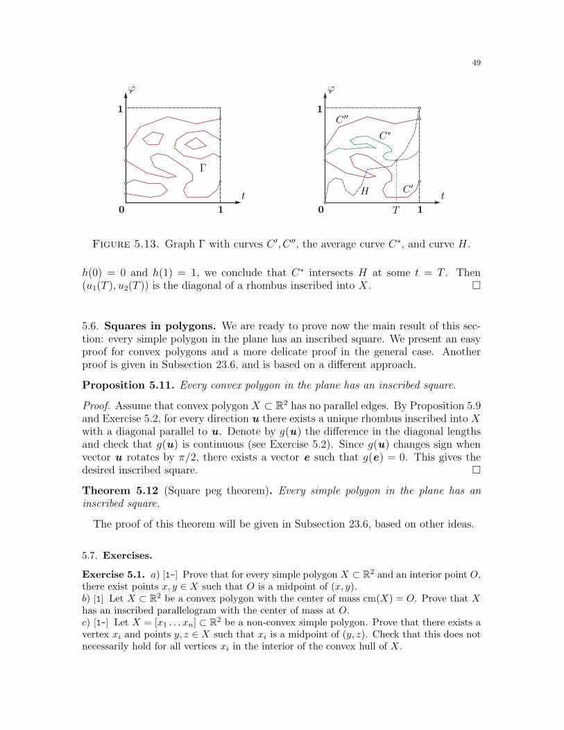
49

00

1

1

1

1 T

tt

ϕϕ

H

Γ

C ′

C ′′

C∗

Figure 5.13. Graph Γ with curves C ′, C ′′, the average curve C∗, and curve H .

h(0) = 0 and h(1) = 1, we conclude that C∗ intersects H at some t = T . Then(u1(T ), u2(T )) is the diagonal of a rhombus inscribed into X.

5.6. Squares in polygons. We are ready to prove now the main result of this sec-tion: every simple polygon in the plane has an inscribed square. We present an easyproof for convex polygons and a more delicate proof in the general case. Anotherproof is given in Subsection 23.6, and is based on a different approach.

Proposition 5.11. Every convex polygon in the plane has an inscribed square.

Proof. Assume that convex polygon X ⊂ R2 has no parallel edges. By Proposition 5.9and Exercise 5.2, for every direction u there exists a unique rhombus inscribed into Xwith a diagonal parallel to u . Denote by g(u) the difference in the diagonal lengthsand check that g(u) is continuous (see Exercise 5.2). Since g(u) changes sign whenvector u rotates by π/2, there exists a vector e such that g(e) = 0. This gives thedesired inscribed square.

Theorem 5.12 (Square peg theorem). Every simple polygon in the plane has aninscribed square.

The proof of this theorem will be given in Subsection 23.6, based on other ideas.

5.7. Exercises.

Exercise 5.1. a) [1-] Prove that for every simple polygon X ⊂ R2 and an interior point O,there exist points x, y ∈ X such that O is a midpoint of (x, y).b) [1] Let X ⊂ R2 be a convex polygon with the center of mass cm(X) = O. Prove that Xhas an inscribed parallelogram with the center of mass at O.c) [1-] Let X = [x1 . . . xn] ⊂ R2 be a non-convex simple polygon. Prove that there exists avertex xi and points y, z ∈ X such that xi is a midpoint of (y, z). Check that this does notnecessarily hold for all vertices xi in the interior of the convex hull of X.

50

Exercise 5.2. (Inscribed rhombi) ♦ a) [1] Prove that every convex polygon in the planewith no parallel edges has at most one inscribed rhombus with a diagonal parallel to a givenline.b) [1] In conditions of a), prove that as the line rotates, the rhombi change continuously.c) [1] Same for inscribed rhombi with an edge parallel to a given line.d) [1] Find examples of polygons with parallel edges which do have inscribed rhombi as inparts a) and b). Prove that whenever a polygon has two such rhombi, it has infinitely manyof them.e) [1-] Find a convex polygon X ⊂ R2 with non-parallel edges and a vertex v, such that Xhas exactly two inscribed rhombi with vertices at v.

Exercise 5.3. a) [1] Let X ⊂ R2 be a simple polygon. Prove that there exist a cyclicquadrilateral (inscribed into a circle) which is inscribed into X, and whose vertices dividethe closed curve X into four arcs of equal length.b) [1] Let X ⊂ R3 be a simple space polygon. Prove that there exist a quadrilateral inscribedinto X whose vertices lie in a plane and divide X into four arcs of equal length.

Exercise 5.4. [1] Let R ⊂ R2 be the Reuleaux triangle defined in Exercise 3.6. Provethat R has no inscribed regular n-gons, for all n ≥ 5.

Exercise 5.5. [1] Let Q1, Q2, Q3 ⊂ R2 be three (non-intersecting) piecewise linear curveswith the same endpoint x and other endpoints y1, y2, and y3, respectively. Let Q = Q1 ∪Q2 ∪ Q3 be the union of these curves. Prove that Q has an inscribed equilateral trianglewith a vertex at either y1, y2 or y3.

Exercise 5.6. [1] Let Q = ∂A, A ⊂ R2 be a simple polygon in the plane and let x1, x2, x3 ∈Q be three distinct points on Q. Prove that there exists a circle inside A which contains atleast one point from the three closed arcs of Q separated by the points xi.

Exercise 5.7. [2-] Let X ⊂ R2 be a simple polygon. Use Exercise 5.5 to prove that for allbut at most two points z ∈ X, there exists an equilateral triangle inscribed into X with avertex at z.

Exercise 5.8. [1-] Prove or disprove: for every convex polygon Q ⊂ R2 containing theorigin O in its relative interior, there exists a triangle inscribed into Q, with the center ofmass at O.

Exercise 5.9. a) [1-] Prove that for every three distinct parallel lines in the plane thereexists an equilateral triangle with a vertex on each line.b) [1] Prove that for every d + 1 distinct parallel hyperplanes in Rd there exists a regularsimplex with a vertex on each hyperplane.c) [1] Prove or disprove: such a simplex is uniquely determined up to a rigid motion.

Exercise 5.10. [1+] Prove that for every three non-intersecting lines ℓ1, ℓ2, ℓ3 ⊂ R3 thereexists a unique triangle ∆ = (a1, a2, a3), such that ai ∈ ℓi and the lines have equal angleswith the adjacent edges of ∆. For example, the angle between ℓ1 and (a1, a2) must be equalto the angle between ℓ1 and (a1, a3).

Exercise 5.11. a) [1-] Prove or disprove: for every simple convex cone C ⊂ R3 thereexists a plane L, such that C ∩ L is an equilateral triangle.b) [1-] Prove or disprove: for every simple convex cone C ⊂ R3 with equal face angles, thereexists a unique plane L, such that C ∩ L is an equilateral triangle.

51

c) [1] Let C be a simple cone with three right face angles. Prove that for every triangle Tthere exists a plane L, such that C ∩ L is congruent to T .d) [1] Prove that every convex cone C ⊂ R3 with four faces there exists a plane L, suchthat C ∩ L is a parallelogram.

Exercise 5.12. a) [1-] Prove that for every tetrahedron ∆ ⊂ R3 there exists a plane L,such that ∆ ∩ L is a rhombus. Prove that there are exactly three such planes.b) [1] Suppose the resulting three rhombi are homothetic. Prove that ∆ is equihedral (seeExercise 25.12).c) [1] Suppose the resulting three rhombi are squares. Prove that ∆ is regular.

Exercise 5.13. [1+] Prove or disprove: every space polygon Q ⊂ R3 has an inscribedrectangle.

Exercise 5.14. [1] Let X ⊂ R2 be a simple polygon in the plane. Prove that there existsa rectangle Q with exactly three vertices of Q lying in X.

Exercise 5.15. Let Q ⊂ R3 be a simple space polygon.a) [2+] Prove that for every k ≥ 3 there exists an equilateral k-gon inscribed into Q. Inother words, prove that there exist distinct points y1, . . . , yk ∈ Q such that

|y1y2| = . . . = |yn−1yn| = |yny1| .b) [∗] Prove that for every k ≥ 3 there exists an equiangular k-gon inscribed into Q. Inother words, prove that there exist distinct points y1, . . . , yk ∈ Q such that

∠ yny1y2 = ∠ y1y2y3 = . . . = ∠ yn−1yny1 .

Exercise 5.16. a) [1+] Prove that for every convex plane polygon and every ρ 6= 1 thereexists at least two inscribed rectangles with aspect ratio (ratio of its sides) equal to ρ.b) [2] Prove that for every simple plane polygon there exists an inscribed rectangle with agiven aspect ratio (ratio of its sides).c) [∗] Let Q ⊂ R2 be an isosceles trapezoid. Prove that for every simple plane polygonthere exists an inscribed polygon similar to Q (equal up to homothety).d) [1] Prove that part c) does not extend to any other quadrilateral Q.

Exercise 5.17. ♦ Let ℓ1, ℓ2, ℓ3 and ℓ4 be generic lines in the plane.a) [1] Prove that there are exactly three squares with all vertices on different lines ℓi.Formalize explicitly what it means to be generic.b) [1] Prove that there are 12 more squares with vertices on lines ℓi.c) [1] Compute the number of rectangles with given aspect ratio (ratio of its sides), suchthat all vertices lie on different lines.d) [1] Let Q ⊂ R2 be a simple quadrilateral with different edge lengths. Compute thenumber of quadrilaterals similar to Q, with all vertices on lines ℓi.

Exercise 5.18. a) [2+] Prove that every simple space polygon in R3 has an inscribed flat(i.e., coplanar) rhombus.b) [1-] Prove that every flat rhombus inscribed into a sphere is a square. Use part a) toconclude that every simple spherical polygon has an inscribed square.c) [2-] Use part b) and a limit argument to give another proof that every simple polygonin the plane has an inscribed square.

Exercise 5.19. An equihedral octahedron Q is defined as a convex hull of three orthogonalintervals (diagonals of Q) intersecting at midpoints. Clearly all eight triangular faces in Qare congruent.

52

a) [1+] Let P ⊂ R3 be a convex polytope which is in general position with respect to theorthogonal axes. Prove that P has an inscribed equihedral octahedron with its diagonalsparallel to the axes.b) [1] Show that the general position condition on P is necessary.c) [1] Find a convex polytope P ⊂ R3 which has at least two inscribed equihedral octahedrawith parallel diagonals.

Exercise 5.20. (Inscribed octahedra) a) [2+] Prove that every convex polytope P ⊂ R3

has an inscribed regular octahedron.b) [2+] Generalize the result to (non-convex) surfaces embedded in R3 and homeomorphicto a sphere.c) [2+] Generalize the result to higher dimensions.

Exercise 5.21. [2-] Find a convex polytope in R3 which has no inscribed bricks (rectan-gular parallelepipeds).

Exercise 5.22. (The table and the chair theorems) Let Q = ∂A, A ⊂ R2 be a convexpolygon, and let f : R2 → R+ be a continuous piecewise linear function which is zero outsideof Q.a) [2+] Prove that for every c > 0 there exist a square of size c, such that cm[x1x2x3x4] ⊂ Aand f(x1) = f(x2) = f(x3) = f(x4).13

b) [2+] Prove that for every triangle ∆ ⊂ R2 there exist a translation ∆′ = [x1x2x3] suchthat cm(∆′) ∈ A and f(x1) = f(x2) = f(x3).14

c) [2-] Prove that part a) does not hold for non-convex A.

Exercise 5.23. (Mountain climbing lemma for general functions) ♦ a) [1-] Show that themountain climbing lemma (Theorem 5.5) does not extend to all continuous functions withthe same boundary conditions.b) [1+] Extend the mountain climbing lemma to all piecewise algebraic functions.

Exercise 5.24. (Generalized mountain climbing lemma) ♦ [1-] Let fi : [0, 1] → [0, 1]be k continuous piecewise linear functions with fi(0) = 0 and fi(1) = 1, for all 1 ≤ i ≤ k.Prove that there exist k continuous piecewise linear functions gi : [0, 1] → [0, 1], such thatgi(0) = 0, gi(1) = 1 for all 1 ≤ i ≤ k, and

f1(g1(t)) = . . . = fk(gk(t)) for every t ∈ [0, 1].

Exercise 5.25. (Ladder problem) [2-] Let C be a piecewise linear curve in the plane whichbegins and ends with a straight unit segment. Prove that there is a continuous family Υ ofunit intervals which are inscribed into C containing both end segments.15

Exercise 5.26. (Ring width problem) [2] Let X ⊂ R2 be a simple polygon with two raysattached as in Figure 5.14. Think of X as if it was made out of metal.a) [2-] A metallic ring of diameter ℓ is an interval of length ℓ whose endpoints lie on differentsides of X. Suppose a metallic ring of diameter ℓ can slide from one ray into another. Provethat so can a metallic ring of diameter ℓ′, for all ℓ′ > ℓ.b) [2-] An elastic ring of diameter ℓ is an interval of length ℓ whose endpoints lie on differentsides of X, and whose length is allowed to decrease to any length smaller than ℓ. Suppose an

13In other words, there is a way to place a table of every size on a hill; thus the “table theorem”.14This is the “chair theorem”.15Thus, two people can coordinate their movements to move along a path while carrying a ladder.

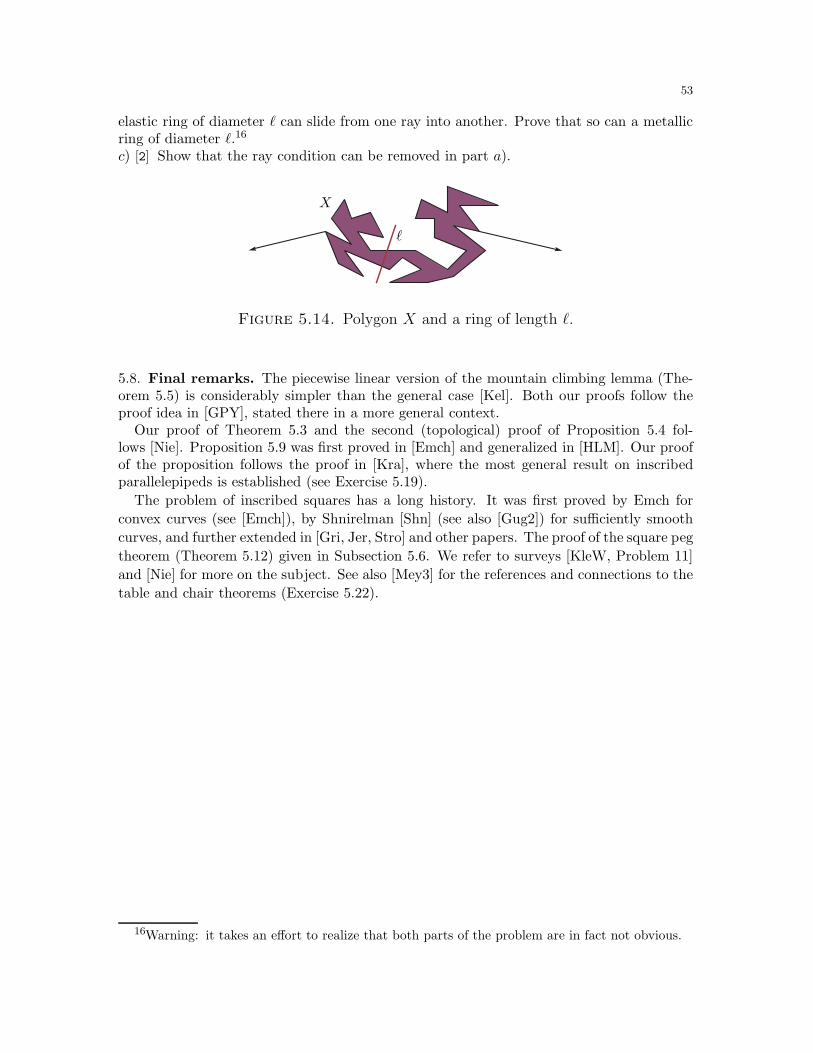
53

elastic ring of diameter ℓ can slide from one ray into another. Prove that so can a metallicring of diameter ℓ.16

c) [2] Show that the ray condition can be removed in part a).

ℓ

X

Figure 5.14. Polygon X and a ring of length ℓ.

5.8. Final remarks. The piecewise linear version of the mountain climbing lemma (The-orem 5.5) is considerably simpler than the general case [Kel]. Both our proofs follow theproof idea in [GPY], stated there in a more general context.

Our proof of Theorem 5.3 and the second (topological) proof of Proposition 5.4 fol-lows [Nie]. Proposition 5.9 was first proved in [Emch] and generalized in [HLM]. Our proofof the proposition follows the proof in [Kra], where the most general result on inscribedparallelepipeds is established (see Exercise 5.19).

The problem of inscribed squares has a long history. It was first proved by Emch for

convex curves (see [Emch]), by Shnirelman [Shn] (see also [Gug2]) for sufficiently smooth

curves, and further extended in [Gri, Jer, Stro] and other papers. The proof of the square peg

theorem (Theorem 5.12) given in Subsection 5.6. We refer to surveys [KleW, Problem 11]

and [Nie] for more on the subject. See also [Mey3] for the references and connections to the

table and chair theorems (Exercise 5.22).

16Warning: it takes an effort to realize that both parts of the problem are in fact not obvious.

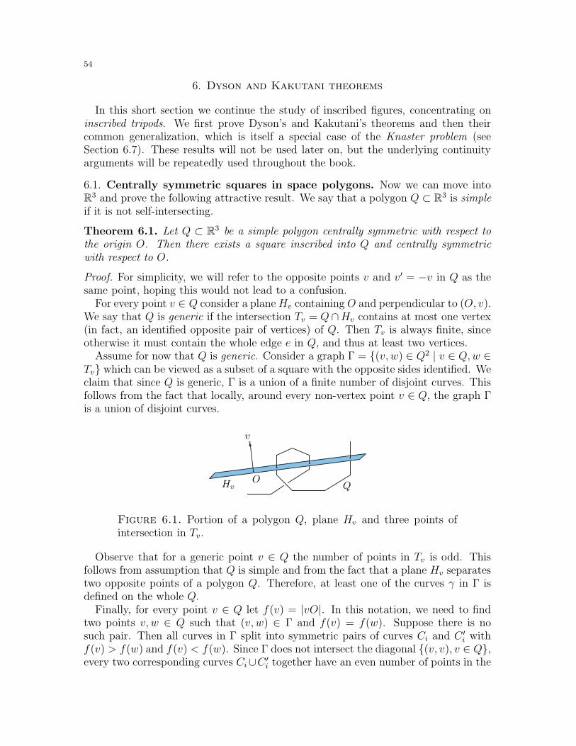
54

6. Dyson and Kakutani theorems

In this short section we continue the study of inscribed figures, concentrating oninscribed tripods. We first prove Dyson’s and Kakutani’s theorems and then theircommon generalization, which is itself a special case of the Knaster problem (seeSection 6.7). These results will not be used later on, but the underlying continuityarguments will be repeatedly used throughout the book.

6.1. Centrally symmetric squares in space polygons. Now we can move intoR3 and prove the following attractive result. We say that a polygon Q ⊂ R3 is simpleif it is not self-intersecting.

Theorem 6.1. Let Q ⊂ R3 be a simple polygon centrally symmetric with respect tothe origin O. Then there exists a square inscribed into Q and centrally symmetricwith respect to O.

Proof. For simplicity, we will refer to the opposite points v and v′ = −v in Q as thesame point, hoping this would not lead to a confusion.

For every point v ∈ Q consider a planeHv containing O and perpendicular to (O, v).We say that Q is generic if the intersection Tv = Q∩Hv contains at most one vertex(in fact, an identified opposite pair of vertices) of Q. Then Tv is always finite, sinceotherwise it must contain the whole edge e in Q, and thus at least two vertices.

Assume for now that Q is generic. Consider a graph Γ = (v, w) ∈ Q2 | v ∈ Q,w ∈Tv which can be viewed as a subset of a square with the opposite sides identified. Weclaim that since Q is generic, Γ is a union of a finite number of disjoint curves. Thisfollows from the fact that locally, around every non-vertex point v ∈ Q, the graph Γis a union of disjoint curves.

O

v

QHv

Figure 6.1. Portion of a polygon Q, plane Hv and three points ofintersection in Tv.

Observe that for a generic point v ∈ Q the number of points in Tv is odd. Thisfollows from assumption that Q is simple and from the fact that a plane Hv separatestwo opposite points of a polygon Q. Therefore, at least one of the curves γ in Γ isdefined on the whole Q.

Finally, for every point v ∈ Q let f(v) = |vO|. In this notation, we need to findtwo points v, w ∈ Q such that (v, w) ∈ Γ and f(v) = f(w). Suppose there is nosuch pair. Then all curves in Γ split into symmetric pairs of curves Ci and C ′

i withf(v) > f(w) and f(v) < f(w). Since Γ does not intersect the diagonal (v, v), v ∈ Q,every two corresponding curves Ci∪C ′

i together have an even number of points in the

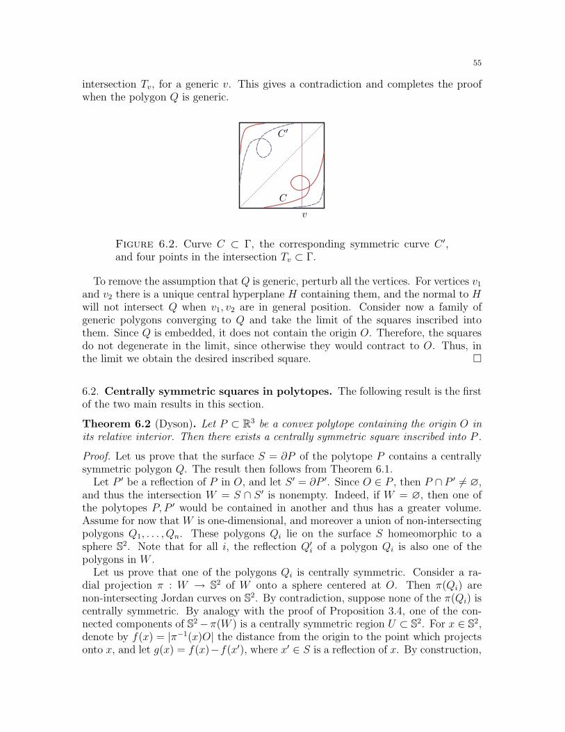
55

intersection Tv, for a generic v. This gives a contradiction and completes the proofwhen the polygon Q is generic.

v

C ′

C

Figure 6.2. Curve C ⊂ Γ, the corresponding symmetric curve C ′,and four points in the intersection Tv ⊂ Γ.

To remove the assumption that Q is generic, perturb all the vertices. For vertices v1

and v2 there is a unique central hyperplane H containing them, and the normal to Hwill not intersect Q when v1, v2 are in general position. Consider now a family ofgeneric polygons converging to Q and take the limit of the squares inscribed intothem. Since Q is embedded, it does not contain the origin O. Therefore, the squaresdo not degenerate in the limit, since otherwise they would contract to O. Thus, inthe limit we obtain the desired inscribed square.

6.2. Centrally symmetric squares in polytopes. The following result is the firstof the two main results in this section.

Theorem 6.2 (Dyson). Let P ⊂ R3 be a convex polytope containing the origin O inits relative interior. Then there exists a centrally symmetric square inscribed into P .

Proof. Let us prove that the surface S = ∂P of the polytope P contains a centrallysymmetric polygon Q. The result then follows from Theorem 6.1.

Let P ′ be a reflection of P in O, and let S ′ = ∂P ′. Since O ∈ P , then P ∩ P ′ 6= ∅,and thus the intersection W = S ∩ S ′ is nonempty. Indeed, if W = ∅, then one ofthe polytopes P, P ′ would be contained in another and thus has a greater volume.Assume for now that W is one-dimensional, and moreover a union of non-intersectingpolygons Q1, . . . , Qn. These polygons Qi lie on the surface S homeomorphic to asphere S2. Note that for all i, the reflection Q′

i of a polygon Qi is also one of thepolygons in W .

Let us prove that one of the polygons Qi is centrally symmetric. Consider a ra-dial projection π : W → S2 of W onto a sphere centered at O. Then π(Qi) arenon-intersecting Jordan curves on S2. By contradiction, suppose none of the π(Qi) iscentrally symmetric. By analogy with the proof of Proposition 3.4, one of the con-nected components of S2−π(W ) is a centrally symmetric region U ⊂ S2. For x ∈ S2,denote by f(x) = |π−1(x)O| the distance from the origin to the point which projectsonto x, and let g(x) = f(x)−f(x′), where x′ ∈ S is a reflection of x. By construction,

56

the function g is continuous and g(x) 6= 0 on U . On the other hand, g(x) = −g(x′)for all x, x′ ∈ U , a contradiction.

Suppose now that the above assumption is false, i.e., that W ⊂ S is not a union ofnon-intersecting polygons. Perturb the vertices of P so that no two faces are paralleland no vertex is opposite to a point on a face. The resulting polytope satisfies theassumption, and the theorem follows by the limit argument.

6.3. Circumscribed cubes. It is natural to assume that Proposition 5.1 can beextended to higher dimensions. This is indeed possible, but the proof is no longerstraightforward. We present only the 3-dimensional case here (see also Exercise 6.12).

We say that a convex set X ⊂ R3 has a circumscribed cube if there exists a cubeC ⊂ R3, such that X ⊆ C and every (2-dimensional) face of C contains a point of X.

Theorem 6.3 (Kakutani). Every convex set X ⊂ R3 has a circumscribed cube.

Proof. Let O ∈ X be the origin, and let S2 be the unit sphere centered at O. Fora point x ∈ S2, denote by f(x) the distance between planes orthogonal to (Ox)and supporting X on both sides. Think of f as a (symmetric) function on a spheref : S2 → R. It suffices to show that there exists three points x, y, z ∈ S2 such that(Ox), (Oy) and (Oz) are orthogonal to each other and such that f(x) = f(y) = f(z).We prove this claim by contradiction.

Think of (xyz) as a right equilateral triangle on S2, i.e., a spherical triangle withedge lengths π/2. For every right equilateral triangle (xyz) ⊂ S3, denote by τ(x, y, z)the orthogonally projection of the point (f(x), f(y), f(z)) ∈ R3 onto the plane L =(a, b, c), a+b+c = 0 ⊂ R3 containing the origin O. Clearly, the map τ is continuousand if f(x) = f(y) = f(z), then τ(x, y, z) = O. We assume that τ(x, y, z) 6= O for allright equilateral triangles.

Fix the three points x0 = (1, 0, 0), y0 = (0, 1, 0) and z0 = (0, 0, 1) in the sphere.Observe that τ(x0, y0, z0), τ(y0, z0, x0) and τ(z0, x0, y0) are equilateral triangles in L.Denote by G = SO(3,R) the group of orthogonal rotations, whose elements can beidentified with the right equilateral triangles (x, y, z) of the same orientation. Considera curve Γ0 ⊂ G which connects (x0, y0, z0) to (y0, z0, x0). Use the symmetry to connect(y0, z0, x0) to (z0, x0, y0) and (z0, x0, y0) to (x0, y0, z0) with the rotations of Γ0. Nowthese three copies of Γ0 form a closed curve Γ1 ⊂ G. Suppose τ(x, y, z) 6= O for everypoint (x, y, z) ∈ Γ1. Denote by γ0 = τ(Γ0) and γ1 = τ(Γ1) the curves in L r O. Byconstruction, γ1 consists of three rotated copies of γ0 (see Figure 6.3). Therefore, theargument of γ1, defined as 2π times the winding number around O, is nonzero and isof the form (3m+ 1)2π.

Finally, recall that G = SO(3,R) is homeomorphic to RP3, and hence the funda-mental group π(G) = Z2. Therefore the curve Γ2 = 2Γ1 is contractible in G. On theother hand, its image γ2 = τ(Γ2) = 2γ1 is not contractible in L r O, a contradic-tion.

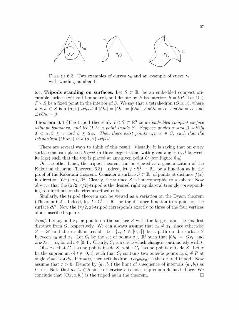
57

γ0

γ0 γ1

O O

Figure 6.3. Two examples of curves γ0 and an example of curve γ1

with winding number 1.

6.4. Tripods standing on surfaces. Let S ⊂ R3 be an embedded compact ori-entable surface (without boundary), and denote by P its interior: S = ∂P . Let O ∈P rS be a fixed point in the interior of S. We say that a tetrahedron (Ouvw), whereu, v, w ∈ S is a (α, β)-tripod if |Ou| = |Ov| = |Ow|, ∠uOv = α, ∠uOw = α, and∠vOw = β.

Theorem 6.4 (The tripod theorem). Let S ⊂ R3 be an embedded compact surfacewithout boundary, and let O be a point inside S. Suppose angles α and β satisfy0 < α, β ≤ π and β ≤ 2α. Then there exist points u, v, w ∈ S, such that thetetrahedron (Ouvw) is a (α, β)-tripod.

There are several ways to think of this result. Visually, it is saying that on everysurface one can place a tripod (a three-legged stand with given angles α, β betweenits legs) such that the top is placed at any given point O (see Figure 6.4).

On the other hand, the tripod theorem can be viewed as a generalization of theKakutani theorem (Theorem 6.3). Indeed, let f : S2 → R+ be a function as in theproof of the Kakutani theorem. Consider a surface S ⊂ R3 of points at distance f(x)in direction (Ox), x ∈ S2. Clearly, the surface S is homeomorphic to a sphere. Nowobserve that the (π/2, π/2)-tripod is the desired right equilateral triangle correspond-ing to directions of the circumscribed cube.

Similarly, the tripod theorem can be viewed as a variation on the Dyson theorem(Theorem 6.2). Indeed, let f : S2 → R+ be the distance function to a point on thesurface ∂P . Now the (π/2, π)-tripod corresponds exactly to three of the four verticesof an inscribed square.

Proof. Let x0 and x1 be points on the surface S with the largest and the smallestdistance from O, respectively. We can always assume that x0 6= x1, since otherwiseS = S2 and the result is trivial. Let xt, t ∈ [0, 1] be a path on the surface Sbetween x0 and x1. Let Ct be the set of points y ∈ R3 such that |Oy| = |Oxt| and∠yOxt = α, for all t ∈ [0, 1]. Clearly, Ct is a circle which changes continuously with t.

Observe that C0 has no points inside S, while C1 has no points outside S. Let τbe the supremum of t ∈ [0, 1], such that Ct contains two outside points at, bt /∈ P atangle β = ∠atObt. If τ = 0, then tetrahedron (Ox0a0b0) is the desired tripod. Nowassume that τ > 0. Denote by (aτ , bτ ) the limit of a sequence of intervals (at, bt) ast→ τ . Note that aτ , bτ ∈ S since otherwise τ is not a supremum defined above. Weconclude that (Oxτaτ bτ ) is the tripod as in the theorem.

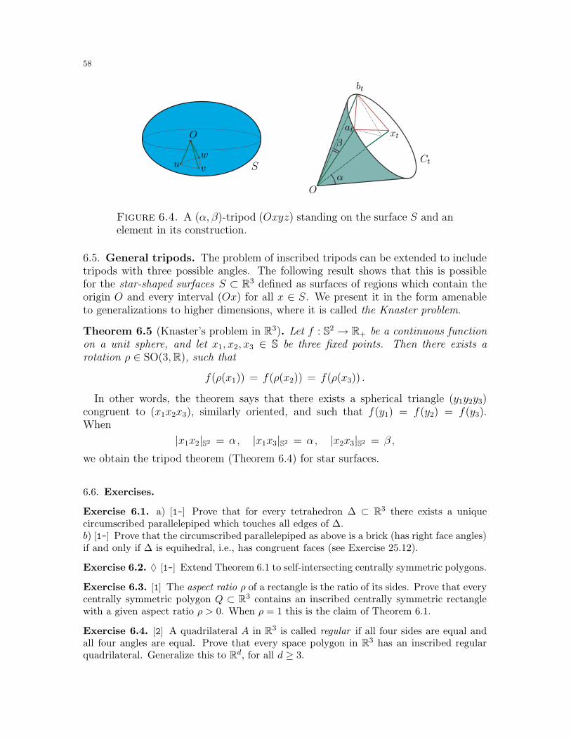
58

u v

w

O

O

S

xt

Ct

at

bt

α

β

Figure 6.4. A (α, β)-tripod (Oxyz) standing on the surface S and anelement in its construction.

6.5. General tripods. The problem of inscribed tripods can be extended to includetripods with three possible angles. The following result shows that this is possiblefor the star-shaped surfaces S ⊂ R3 defined as surfaces of regions which contain theorigin O and every interval (Ox) for all x ∈ S. We present it in the form amenableto generalizations to higher dimensions, where it is called the Knaster problem.

Theorem 6.5 (Knaster’s problem in R3). Let f : S2 → R+ be a continuous functionon a unit sphere, and let x1, x2, x3 ∈ S be three fixed points. Then there exists arotation ρ ∈ SO(3,R), such that

f(ρ(x1)) = f(ρ(x2)) = f(ρ(x3)) .

In other words, the theorem says that there exists a spherical triangle (y1y2y3)congruent to (x1x2x3), similarly oriented, and such that f(y1) = f(y2) = f(y3).When

|x1x2|S2 = α, |x1x3|S2 = α, |x2x3|S2 = β ,

we obtain the tripod theorem (Theorem 6.4) for star surfaces.

6.6. Exercises.

Exercise 6.1. a) [1-] Prove that for every tetrahedron ∆ ⊂ R3 there exists a uniquecircumscribed parallelepiped which touches all edges of ∆.b) [1-] Prove that the circumscribed parallelepiped as above is a brick (has right face angles)if and only if ∆ is equihedral, i.e., has congruent faces (see Exercise 25.12).

Exercise 6.2. ♦ [1-] Extend Theorem 6.1 to self-intersecting centrally symmetric polygons.

Exercise 6.3. [1] The aspect ratio ρ of a rectangle is the ratio of its sides. Prove that everycentrally symmetric polygon Q ⊂ R3 contains an inscribed centrally symmetric rectanglewith a given aspect ratio ρ > 0. When ρ = 1 this is the claim of Theorem 6.1.

Exercise 6.4. [2] A quadrilateral A in R3 is called regular if all four sides are equal andall four angles are equal. Prove that every space polygon in R3 has an inscribed regularquadrilateral. Generalize this to Rd, for all d ≥ 3.

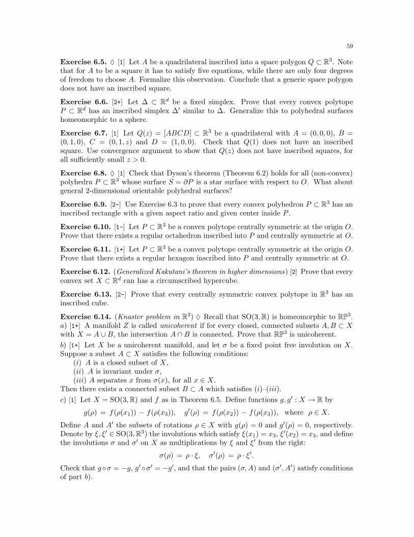
59

Exercise 6.5. ♦ [1] Let A be a quadrilateral inscribed into a space polygon Q ⊂ R3. Notethat for A to be a square it has to satisfy five equations, while there are only four degreesof freedom to choose A. Formalize this observation. Conclude that a generic space polygondoes not have an inscribed square.

Exercise 6.6. [2+] Let ∆ ⊂ Rd be a fixed simplex. Prove that every convex polytopeP ⊂ Rd has an inscribed simplex ∆′ similar to ∆. Generalize this to polyhedral surfaceshomeomorphic to a sphere.

Exercise 6.7. [1] Let Q(z) = [ABCD] ⊂ R3 be a quadrilateral with A = (0, 0, 0), B =(0, 1, 0), C = (0, 1, z) and D = (1, 0, 0). Check that Q(1) does not have an inscribedsquare. Use convergence argument to show that Q(z) does not have inscribed squares, forall sufficiently small z > 0.

Exercise 6.8. ♦ [1] Check that Dyson’s theorem (Theorem 6.2) holds for all (non-convex)polyhedra P ⊂ R3 whose surface S = ∂P is a star surface with respect to O. What aboutgeneral 2-dimensional orientable polyhedral surfaces?

Exercise 6.9. [2-] Use Exercise 6.3 to prove that every convex polyhedron P ⊂ R3 has aninscribed rectangle with a given aspect ratio and given center inside P .

Exercise 6.10. [1-] Let P ⊂ R3 be a convex polytope centrally symmetric at the origin O.Prove that there exists a regular octahedron inscribed into P and centrally symmetric at O.

Exercise 6.11. [1+] Let P ⊂ R3 be a convex polytope centrally symmetric at the origin O.Prove that there exists a regular hexagon inscribed into P and centrally symmetric at O.

Exercise 6.12. (Generalized Kakutani’s theorem in higher dimensions) [2] Prove that everyconvex set X ⊂ Rd can has a circumscribed hypercube.

Exercise 6.13. [2-] Prove that every centrally symmetric convex polytope in R3 has aninscribed cube.

Exercise 6.14. (Knaster problem in R3) ♦ Recall that SO(3,R) is homeomorphic to RP3.a) [1+] A manifold Z is called unicoherent if for every closed, connected subsets A,B ⊂ Xwith X = A ∪B, the intersection A ∩B is connected. Prove that RP3 is unicoherent.

b) [1+] Let X be a unicoherent manifold, and let σ be a fixed point free involution on X.Suppose a subset A ⊂ X satisfies the following conditions:

(i) A is a closed subset of X,(ii) A is invariant under σ,(iii) A separates x from σ(x), for all x ∈ X.

Then there exists a connected subset B ⊂ A which satisfies (i)–(iii).

c) [1] Let X = SO(3,R) and f as in Theorem 6.5. Define functions g, g′ : X → R by

g(ρ) = f(ρ(x1)) − f(ρ(x3)), g′(ρ) = f(ρ(x2)) − f(ρ(x3)), where ρ ∈ X.Define A and A′ the subsets of rotations ρ ∈ X with g(ρ) = 0 and g′(ρ) = 0, respectively.Denote by ξ, ξ′ ∈ SO(3,R3) the involutions which satisfy ξ(x1) = x3, ξ′(x2) = x3, and definethe involutions σ and σ′ on X as multiplications by ξ and ξ′ from the right:

σ(ρ) = ρ · ξ, σ′(ρ) = ρ · ξ′.Check that gσ = −g, g′ σ′ = −g′, and that the pairs (σ,A) and (σ′, A′) satisfy conditionsof part b).

60

d) [1] Denote by B ⊂ A and B′ ⊂ A′ the connected subsets obtained by applying part b)to sets A and A′ in part c). Assume that B ∩B′ = ∅. Use the fact that σ, σ′ preserve theHaar measure on SO(3,R) to obtain a contradiction. Conclude from here Theorem 6.5.

Exercise 6.15. (General tripods on surfaces) ♦ [∗] Let S ⊂ R3 be an embedded orientablesurface and let O be a point inside S. For a simple cone C with face angles α, β and γ,define a (α, β, γ)-tripod on S to be a triple of points u, v,w ∈ S, such that the tetrahedron(Ouvw) has ∠uOv = α, ∠ vOw = β, ∠wOv = γ, and |Ou| = |Ov| = |Ow|. Prove that forevery C as above, there exists a (α, β, γ)-tripod on S.

6.7. Final remarks. Kakutani’s theorem (Theorem 6.3) was proved in [Kaku] and becamea source of inspiration for a number of results. It was extended in [YamY] to higher dimen-sions (Exercise 6.12). Our version of Dyson’s theorem is different from the original [Dys],and can be viewed as a variation on Kakutani’s theorem. Dyson noticed that in the proofKakutani never used the fact that f is centrally symmetric, so he showed that general func-tions on spheres always have two orthogonal diameters such that the function is constanton all four endpoints. This result, in turn, was also extended in a number of ways (see e.g.Exercise 6.8 and 6.9).

Our proof of the tripod theorem (Theorem 6.4) is based on [Gor], which in turn followsthe proof in [YamY]. Theorem 6.5 is due to Floyd who used a topological argument toprove it [Flo]. The proof is outlined in Exercise 6.14. The generalization to all embedded2-dimensional surfaces is stated as Exercise 6.15.

Knaster’s problem was formulated by B. Knaster in 1947 in an attempt to further gen-eralize the Kakutani theorem. Namely, he conjectured that for every f : Sd → Rm andx1, . . . , xn ∈ Sd, where n = d − m + 2, there exists a rotation ρ ∈ SO(m,R) such thatf(ρ(x1)) = . . . = f(ρ(xn)). This conjecture was refuted in a number of cases, for examplefor all d > m > 2 [Chen], but remained open for m = 1 until recently, when it was disprovedfor d > 1012 [KasS].

61

7. Geometric inequalities

The isoperimetric problems are some of the oldest problems in geometry. Thereare numerous monographs written on the subject, so we see little need to expandon this (see Subsection 7.9). We do need, however, the important Brunn–Minkowskiinequality, including the equality part of it, to prove the Minkowski theorem in Sec-tion 36. Thus, we present an elementary introduction to the subject, trying to makeit as painless as possible.

7.1. Isoperimetry in the plane. It is well known that among all regions in theplane with the same area, the disk has the smallest perimeter. Proving this result isactually more delicate than it seems at first sight. The following proof due to Steineris beautiful, but also (somewhat) incorrect. While we explain the problem in the nextsubsection, it is a nice exercise to find the error.

Throughout this section we always assume that our sets are convex. This allowsus to avoid certain unpleasantness in dealing with general compact sets.17

Theorem 7.1 (Isoperimetric inequality in the plane). Among all convex sets in theplane with a given area, the disk has the smallest perimeter.

Incorrect proof of Theorem 7.1. The proof can be split into several easy steps. LetX ⊂ R2 be a compact set in the plane. We say that the set is optimal if it mini-mizes the perimeter given the area. We will try to characterize the optimal sets andeventually show that only a disk can be optimal.

1) We say that two points x and y on the boundary P = ∂X are opposite if theydivide P into two equal halves. The interval (xy) is called a diameter in this case.We claim that in an optimal set X the diameter divides the area into two equal parts.If not, attach the bigger part and its reflection to obtain a set Y of equal perimeterand bigger area (see Figure 7.1).

2) Let (xy) be a diameter in an optimal set X, and let P = ∂X. For everypoint z ∈ P we then have ∠xzy = π/2. Indeed, from 1) the diameter splits the areainto equal parts. If ∠xzy 6= π/2, take chords [xy], [yz] and denote by A,B the regionsthey separate as in the figure. Now attach A and B to a triangle (x′y′z′) with sides|x′z′| = |xz|, |z′y′| = |zy|, and ∠x′y′z′ = π/2. Copy the construction symmetricallyon the other side of the diameter (see Figure 7.1). Since area(xyz) < area(x′y′z′) andareas of segments remain the same, we obtain a region X ′ with the same perimeterand bigger area.

In summary, we showed that in an optimal set the angle at all points of the bound-ary to a fixed diameter must be π/2. Thus X is a circle. This completes the proof.

17Otherwise, we have to specify that our set X is measurable, has a measurable boundary, etc.For all purposes in this section the reader can assume that X has a piecewise analytic boundary.Then it is easy to show that the convex hull conv(X) has a smaller perimeter but a bigger area, thusreducing the problem to the convex case.

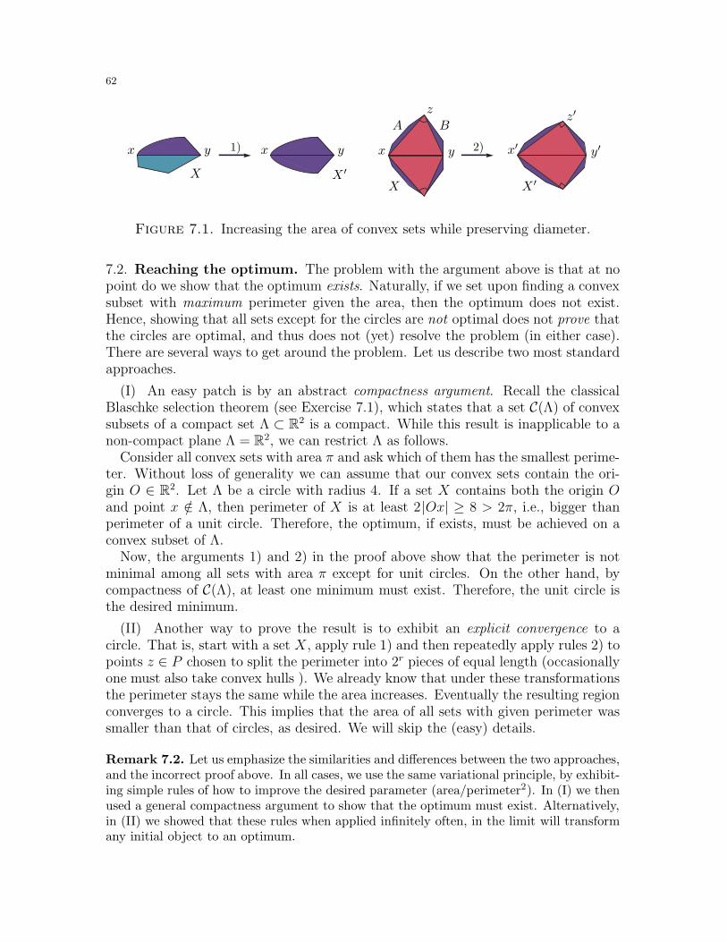
62

1) 2)

XX

X ′X ′

A B

xx x yy y

z

x′ y′

z′

Figure 7.1. Increasing the area of convex sets while preserving diameter.

7.2. Reaching the optimum. The problem with the argument above is that at nopoint do we show that the optimum exists. Naturally, if we set upon finding a convexsubset with maximum perimeter given the area, then the optimum does not exist.Hence, showing that all sets except for the circles are not optimal does not prove thatthe circles are optimal, and thus does not (yet) resolve the problem (in either case).There are several ways to get around the problem. Let us describe two most standardapproaches.

(I) An easy patch is by an abstract compactness argument. Recall the classicalBlaschke selection theorem (see Exercise 7.1), which states that a set C(Λ) of convexsubsets of a compact set Λ ⊂ R2 is a compact. While this result is inapplicable to anon-compact plane Λ = R2, we can restrict Λ as follows.

Consider all convex sets with area π and ask which of them has the smallest perime-ter. Without loss of generality we can assume that our convex sets contain the ori-gin O ∈ R2. Let Λ be a circle with radius 4. If a set X contains both the origin Oand point x /∈ Λ, then perimeter of X is at least 2|Ox| ≥ 8 > 2π, i.e., bigger thanperimeter of a unit circle. Therefore, the optimum, if exists, must be achieved on aconvex subset of Λ.

Now, the arguments 1) and 2) in the proof above show that the perimeter is notminimal among all sets with area π except for unit circles. On the other hand, bycompactness of C(Λ), at least one minimum must exist. Therefore, the unit circle isthe desired minimum.

(II) Another way to prove the result is to exhibit an explicit convergence to acircle. That is, start with a set X, apply rule 1) and then repeatedly apply rules 2) topoints z ∈ P chosen to split the perimeter into 2r pieces of equal length (occasionallyone must also take convex hulls ). We already know that under these transformationsthe perimeter stays the same while the area increases. Eventually the resulting regionconverges to a circle. This implies that the area of all sets with given perimeter wassmaller than that of circles, as desired. We will skip the (easy) details.

Remark 7.2. Let us emphasize the similarities and differences between the two approaches,and the incorrect proof above. In all cases, we use the same variational principle, by exhibit-ing simple rules of how to improve the desired parameter (area/perimeter2). In (I) we thenused a general compactness argument to show that the optimum must exist. Alternatively,in (II) we showed that these rules when applied infinitely often, in the limit will transformany initial object to an optimum.

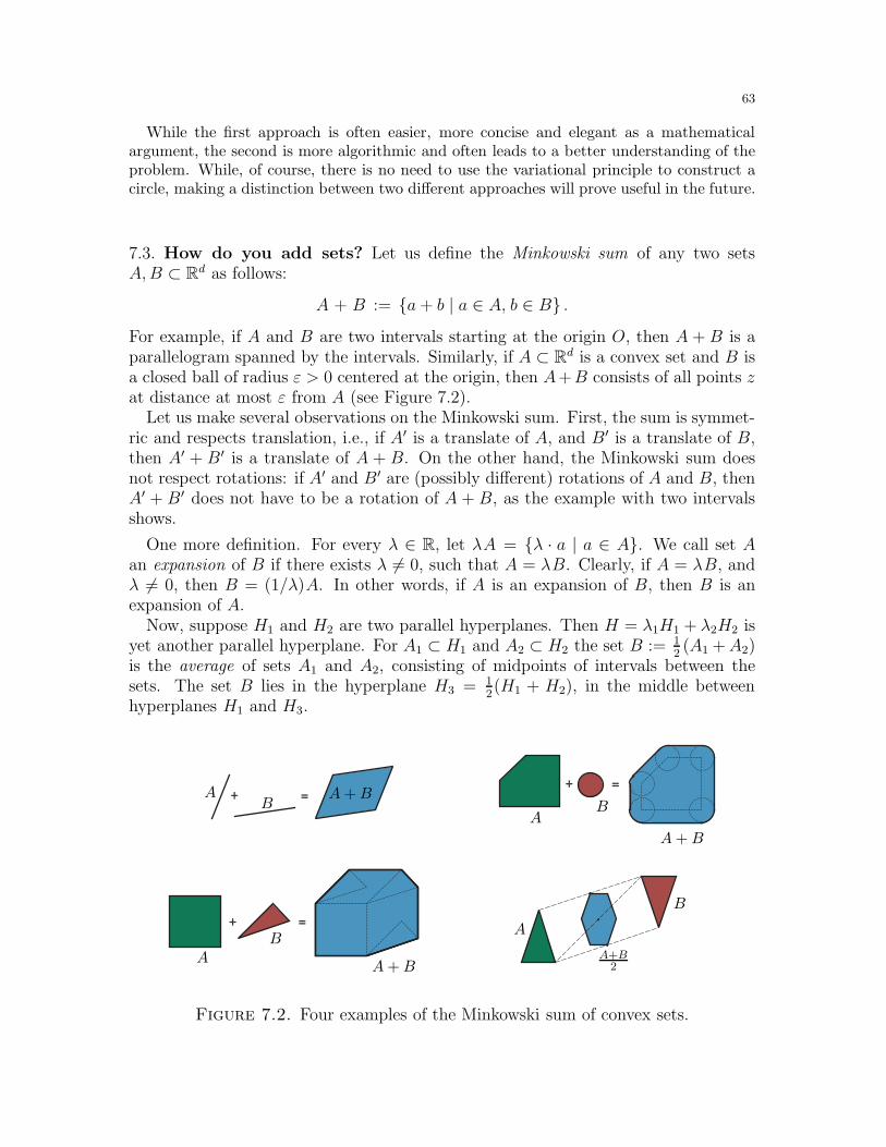
63

While the first approach is often easier, more concise and elegant as a mathematicalargument, the second is more algorithmic and often leads to a better understanding of theproblem. While, of course, there is no need to use the variational principle to construct acircle, making a distinction between two different approaches will prove useful in the future.

7.3. How do you add sets? Let us define the Minkowski sum of any two setsA,B ⊂ Rd as follows:

A + B := a+ b | a ∈ A, b ∈ B .For example, if A and B are two intervals starting at the origin O, then A + B is aparallelogram spanned by the intervals. Similarly, if A ⊂ Rd is a convex set and B isa closed ball of radius ε > 0 centered at the origin, then A+B consists of all points zat distance at most ε from A (see Figure 7.2).

Let us make several observations on the Minkowski sum. First, the sum is symmet-ric and respects translation, i.e., if A′ is a translate of A, and B′ is a translate of B,then A′ + B′ is a translate of A + B. On the other hand, the Minkowski sum doesnot respect rotations: if A′ and B′ are (possibly different) rotations of A and B, thenA′ + B′ does not have to be a rotation of A + B, as the example with two intervalsshows.

One more definition. For every λ ∈ R, let λA = λ · a | a ∈ A. We call set Aan expansion of B if there exists λ 6= 0, such that A = λB. Clearly, if A = λB, andλ 6= 0, then B = (1/λ)A. In other words, if A is an expansion of B, then B is anexpansion of A.

Now, suppose H1 and H2 are two parallel hyperplanes. Then H = λ1H1 + λ2H2 isyet another parallel hyperplane. For A1 ⊂ H1 and A2 ⊂ H2 the set B := 1

2(A1 +A2)

is the average of sets A1 and A2, consisting of midpoints of intervals between thesets. The set B lies in the hyperplane H3 = 1

2(H1 + H2), in the middle between

hyperplanes H1 and H3.

+ =

+ =

+ =A

A

A

A

B

B

BB

A+B

A+B

A+B

A+B2

Figure 7.2. Four examples of the Minkowski sum of convex sets.

64

Recall that by area(S) = vold−1(S) we denote the (d − 1)-dimensional volume ofthe surface S ⊂ Rd. The following result expresses the area of S via the volume ofthe Minkowski sums.

Proposition 7.3. Let X ⊂ Rd be a convex set with the surface S = ∂X, and let Bbe a unit ball. Then:

area(S) =d

dtvol(X + tB)

∣∣t=0

.

The proof is clear for polytopes and requires a straightforward convergence argu-ment for general sets. In fact, everywhere below the reader can use this propositionas a definition of the surface area of general convex sets.

7.4. Slicing polytopes with hyperplanes. The following theorem is the key resultin the field, marking the beginning of modern studies of geometric inequalities. Wewill need it to solve the isoperimetric problem in Rd, and later on to prove theMinkowski uniqueness theorem (see Section 36).

Theorem 7.4 (Brunn–Minkowski inequality). Let A,B ⊂ Rd be two convex bodies.Then

vol(A+B)1/d ≥ vol(A)1/d + vol(B)1/d .

Moreover, the inequality becomes an equality only if A is an expansion of B.

We prove in this section only the first part of the theorem. The second part isproved in the Appendix (see Subsection 41.5).

The following interesting result is actually a corollary from the Brunn–Minkowskiinequality. It was, in fact, the original motivation for Brunn’s studies (the workof Minkowski came later). We deduce this theorem from Theorem 7.4 in the nextsubsection.

Theorem 7.5 (Brunn). Let P be a convex body and let H1, H2 and H3 be three parallelhyperplanes in Rd intersecting P in that order. Denote by Ai = P ∩Hi, 1 ≤ i ≤ 3.Then: area(A2) ≥ minarea(A1); area(A3).Example 7.6. Suppose d = 2 and line H2 is a midway between H1 and H3. Then a strongerstatement is true: area(A2) ≥

(area(A1)+area(A3)

)/2. On the other hand, taking averages

is not useful in higher dimensions. Take a simplex P = 0 ≤ x1 ≤ x2 ≤ . . . ≤ xd ≤ 1 ⊂ Rd,and let Hi be the hyperplanes defined by linear equations x1 = ai, where a1 = 0, a2 = 1

2 ,and a3 = 1. Clearly, the hyperplanes are parallel and at equal distance from each other.On the other hand, the areas of the intersections are given by

area(A1) = 0 , area(A2) =1

2dn!, and area(A3) =

1

n!.

Thus, the best we can hope for is area(A2) ≥(area(A1) + area(A3)

)/2d, an unattractive

inequality formally not implying Brunn’s theorem. On the other hand, this does suggestthat taking d-th root is a good idea, since in this case we have area(A2)1/d =

(area(A1)1/d+

area(A3)1/d)/2.

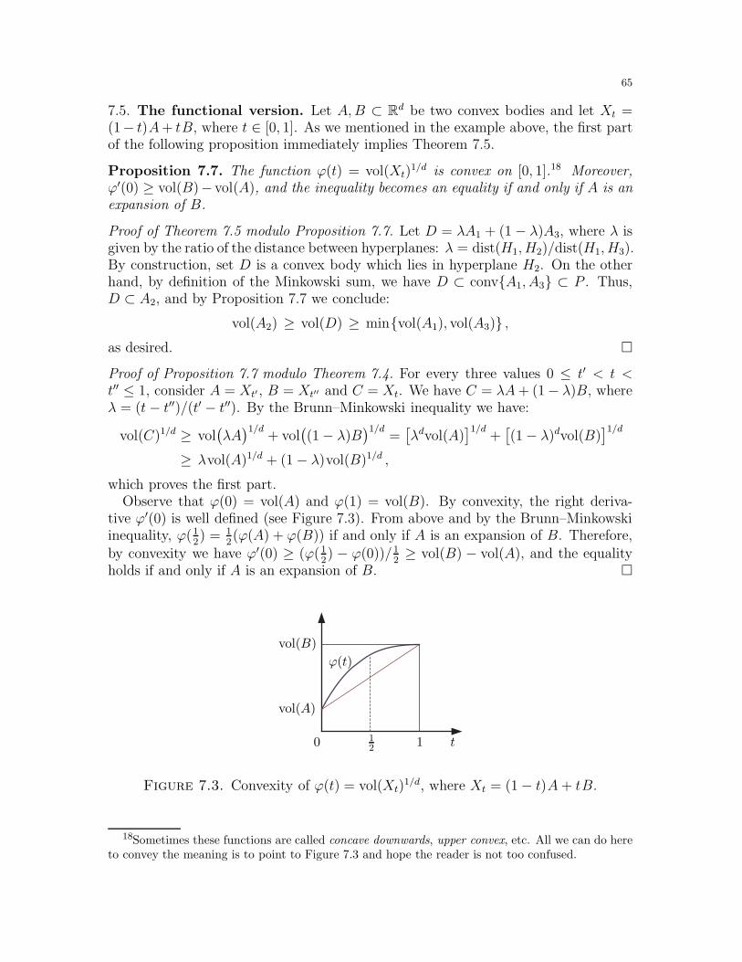
65

7.5. The functional version. Let A,B ⊂ Rd be two convex bodies and let Xt =(1− t)A+ tB, where t ∈ [0, 1]. As we mentioned in the example above, the first partof the following proposition immediately implies Theorem 7.5.

Proposition 7.7. The function ϕ(t) = vol(Xt)1/d is convex on [0, 1].18 Moreover,

ϕ′(0) ≥ vol(B)− vol(A), and the inequality becomes an equality if and only if A is anexpansion of B.

Proof of Theorem 7.5 modulo Proposition 7.7. Let D = λA1 + (1− λ)A3, where λ isgiven by the ratio of the distance between hyperplanes: λ = dist(H1, H2)/dist(H1, H3).By construction, set D is a convex body which lies in hyperplane H2. On the otherhand, by definition of the Minkowski sum, we have D ⊂ convA1, A3 ⊂ P . Thus,D ⊂ A2, and by Proposition 7.7 we conclude:

vol(A2) ≥ vol(D) ≥ minvol(A1), vol(A3) ,as desired.

Proof of Proposition 7.7 modulo Theorem 7.4. For every three values 0 ≤ t′ < t <t′′ ≤ 1, consider A = Xt′ , B = Xt′′ and C = Xt. We have C = λA+ (1− λ)B, whereλ = (t− t′′)/(t′ − t′′). By the Brunn–Minkowski inequality we have:

vol(C)1/d ≥ vol(λA)1/d

+ vol((1− λ)B

)1/d=[λdvol(A)

]1/d+[(1− λ)dvol(B)

]1/d

≥ λvol(A)1/d + (1− λ)vol(B)1/d ,

which proves the first part.Observe that ϕ(0) = vol(A) and ϕ(1) = vol(B). By convexity, the right deriva-

tive ϕ′(0) is well defined (see Figure 7.3). From above and by the Brunn–Minkowskiinequality, ϕ(1

2) = 1

2(ϕ(A) + ϕ(B)) if and only if A is an expansion of B. Therefore,

by convexity we have ϕ′(0) ≥ (ϕ(12) − ϕ(0))/1

2≥ vol(B) − vol(A), and the equality

holds if and only if A is an expansion of B.

0 112 t

ϕ(t)

vol(A)

vol(B)

Figure 7.3. Convexity of ϕ(t) = vol(Xt)1/d, where Xt = (1− t)A+ tB.

18Sometimes these functions are called concave downwards, upper convex, etc. All we can do hereto convey the meaning is to point to Figure 7.3 and hope the reader is not too confused.

66

7.6. The general isoperimetric inequality. Here is the main result in this section:

Theorem 7.8 (Isoperimetric inequality in Rd). Among all convex sets in Rd with agiven volume, the ball has the smallest surface area.

Proof. Let A be a convex set, and let B be a unit ball in Rd. By Proposition 7.7, thefunction ϕ(t) = vol

((1− t)A+ tB) is convex on [0, 1]. Therefore, by Proposition 7.3

we obtain:

area(A) =d

dtvol(A+ tB)

∣∣t=0

=d

dt

[(1 + t)d vol

(A

1 + t+

tB

1 + t

)] ∣∣∣t=0

=d

dt

[(1 + t)ϕ

(t

1 + t

)]d ∣∣∣t=0

= d ϕ(0)d−1[ϕ(0) + ϕ′(0)

].

By Proposition 7.7, we have ϕ′(0) ≥ vol(B) − vol(A), and the inequality becomesan equality if and only if A is an expansion of B. Since vol(A) = ϕ(0), the area(A)minimizes only when A is an expansion of B, i.e., when A is a ball.

Remark 7.9. In the spirit of Remark 7.2, it is instructive to decide what type of argumentis used in this proof: did we use a compactness or an explicit convergence argument? Fromabove, the rule for decreasing ψ(X) = area(X)/vol(X)(d−1)/d turns out to be quite simple:take Xt = (1 − t)X + tB, where B is a unit ball. Letting t → 1 makes Xt approach theunit ball. Thus the proof can be viewed as an explicit convergence argument, perhaps anextremely simple case of it.

7.7. Brick-by-brick proof of the Brunn–Minkowski inequality. Perhaps sur-prisingly, the proof of Theorem 7.4 will proceed by induction. Formally, let us provethe inequality for brick regions defined as disjoint unions of bricks (parallelepipedswith edges parallel to the coordinate axes). Note that we drop the convexity condi-tion. A union of bricks does not have to be connected or the bricks be of the samesize: any disjoint union of bricks will do (see Figure 7.4). Denote by Bd the set of allbrick regions in Rd.

Lemma 7.10. If the Brunn–Minkowski inequality holds for brick regions A,B ∈ Bd,it also holds for general convex regions in Rd.

We continue with the proof of the inequality. The lemma will be proved later.

Proof of the Brunn–Minkowski inequality for brick regions. Let A andB be two brickregions. We use induction on the total number k of bricks in A and B. For the base ofinduction, suppose k = 2, so both sets consist of single bricks: A = [x1×x2× . . .×xd]and B = [y1 × y2 × . . . × yd]. The Brunn–Minkowski inequality then becomes theMinkowski inequality19 (Theorem 41.4).

For the induction step, suppose the result holds for brick regions with k or fewerbricks (in total), k ≥ 2. Now, take two brick regions A,B ∈ Bd with k + 1 bricks.Suppose A contains at least two bricks (otherwise we can relabel the regions). Fix

19While we move the proof of the Minkowski inequality to the appendix as a standard result, wedo suggest the reader go over the proof so as to acquaint yourself with the proof style of inequalities.

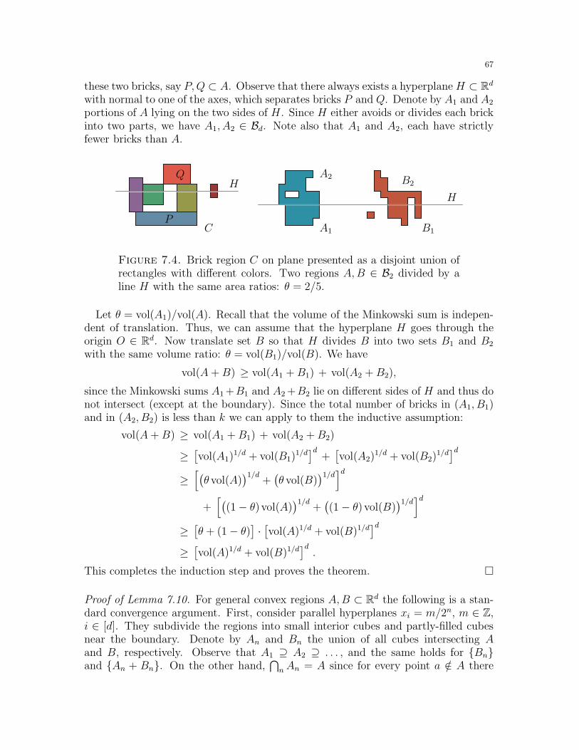
67

these two bricks, say P,Q ⊂ A. Observe that there always exists a hyperplane H ⊂ Rdwith normal to one of the axes, which separates bricks P and Q. Denote by A1 and A2

portions of A lying on the two sides of H . Since H either avoids or divides each brickinto two parts, we have A1, A2 ∈ Bd. Note also that A1 and A2, each have strictlyfewer bricks than A.

A1 B1

A2 B2

C

HH

P

Q

Figure 7.4. Brick region C on plane presented as a disjoint union ofrectangles with different colors. Two regions A,B ∈ B2 divided by aline H with the same area ratios: θ = 2/5.

Let θ = vol(A1)/vol(A). Recall that the volume of the Minkowski sum is indepen-dent of translation. Thus, we can assume that the hyperplane H goes through theorigin O ∈ Rd. Now translate set B so that H divides B into two sets B1 and B2

with the same volume ratio: θ = vol(B1)/vol(B). We have

vol(A+B) ≥ vol(A1 +B1) + vol(A2 +B2),

since the Minkowski sums A1 +B1 and A2 +B2 lie on different sides of H and thus donot intersect (except at the boundary). Since the total number of bricks in (A1, B1)and in (A2, B2) is less than k we can apply to them the inductive assumption:

vol(A+B) ≥ vol(A1 +B1) + vol(A2 +B2)

≥[vol(A1)

1/d + vol(B1)1/d]d

+[vol(A2)

1/d + vol(B2)1/d]d

≥[(θ vol(A)

)1/d+(θ vol(B)

)1/d]d

+[(

(1− θ) vol(A))1/d

+((1− θ) vol(B)

)1/d]d

≥[θ + (1− θ)

]·[vol(A)1/d + vol(B)1/d

]d

≥[vol(A)1/d + vol(B)1/d

]d.

This completes the induction step and proves the theorem.

Proof of Lemma 7.10. For general convex regions A,B ⊂ Rd the following is a stan-dard convergence argument. First, consider parallel hyperplanes xi = m/2n, m ∈ Z,i ∈ [d]. They subdivide the regions into small interior cubes and partly-filled cubesnear the boundary. Denote by An and Bn the union of all cubes intersecting Aand B, respectively. Observe that A1 ⊇ A2 ⊇ . . . , and the same holds for Bnand An + Bn. On the other hand,

⋂nAn = A since for every point a /∈ A there

68

exists an ε > 0, such that a cube with side ε containing a does not intersect A. Thisgives vol(An) → vol(A) and vol(Bn) → vol(B), as n → ∞. In the topology definedby the distance d(A,B) (see Exercise 7.1), this implies that An → A and Bn → B,as n→∞.

Finally, A+B ⊇⋂n An+Bn since for every cn = an+bn → c ∈ Rd, by compactness

of A,B there exist converging subsequences an → a and bn → b, and thus c = a+ b ∈A + B. On the other hand, An + Bn ⊇ A + B for all n ∈ N, which implies thatAn + Bn → A + B as n → ∞. Now we can apply the inequality to the brickregions An and Bn:

vol(A+B)1/d = limn→∞

vol(An +Bn)1/d ≥ lim

n→∞vol(An)

1/d + limn→∞

vol(Bn)1/d

≥ vol(A)1/d + vol(B)1/d ,

which completes the proof of the lemma.

7.8. Exercises.

Exercise 7.1. (Blaschke selection theorem) ♦ [1+] For every subset Λ ⊂ Rd, let C(Λ) be theset of convex subsets of Λ. Define a distance d(X,Y ) between two convex sets X,Y ⊂ C(Rd)as follows:

d(X,Y ) := vol(X r Y ) + vol(Y rX).

Check that d(X,Y ) is a metric on C(Rd). Prove that C(Λ) ⊂ C(Rd) is compact if and onlyif set Λ ⊂ Rd is compact. Conclude that an infinite family of convex subsets inside a unitcube has a converging subsequence.

Exercise 7.2. Let X ⊂ R3 be a convex polytope. Define ρ(X) to be the set of pointsobtained by reflections of one point in X across another: ρ(X) = 2x− y | x, y ∈ X .a) [1-] Show that ρ(X) is also a convex polytope.b) [1-] Consider a sequence X1,X2, . . ., where Xi+1 = ρ(Xi) and X1 is a cube. Computepolytope Xn for all n > 1.c) [1] Same question when X1 is a regular tetrahedron, octahedron and icosahedron.d) [1] Same question when X1 is a standard tetrahedron and a Hill tetrahedron (see Sub-section 31.6).e) [1] Prove or disprove: for every fixed X1, the number of faces of Xn is bounded, asn→∞.f) [1+] Scale polytopes Yn to have the same unit volume: Yn = Xn/vol(Xn). Prove thatthe sequence Yn converges to a convex body.

Exercise 7.3. (Steiner symmetrization) Another one of several Steiner’s ingenious proofsof the isoperimetry in the plane is based on the following construction. Take a convex setX ⊂ R2 and any line ℓ. Divide X into infinitely many intervals [a, b], a, b ∈ ∂X, orthogonalto ℓ. Move each interval [a, b] along the line (a, b) so that it is symmetric with respect to ℓ(See Figure 7.5). Denote by Y = S(X, ℓ) the resulting set. The resulting map ς : X → Yis called the Steiner symmetrization.a) [1] Prove that diam(Y ) ≤ diam(X), area(Y ) = area(X) and perimeter(Y ) ≤ perimeter(X).b) [1+] Prove that C = ς(A) + ς(B) fits inside D = ς(A+B), for all convex A,B ⊂ R2.c) [1] Prove that C is a translate of D if and only if A and B are homothetic.

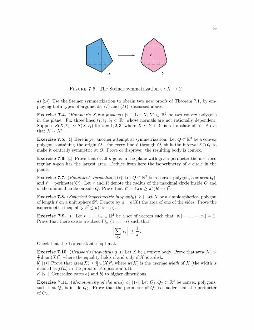
69

X Y

ℓℓ

Figure 7.5. The Steiner symmetrization ς : X → Y .

d) [1+] Use the Steiner symmetrization to obtain two new proofs of Theorem 7.1, by em-ploying both types of arguments, (I) and (II), discussed above.

Exercise 7.4. (Hammer’s X-ray problem) [2-] Let X,X ′ ⊂ R2 be two convex polygonsin the plane. Fix three lines ℓ1, ℓ2, ℓ3 ⊂ R2 whose normals are not rationally dependent.Suppose S(X, ℓi) ∼ S(X, ℓi) for i = 1, 2, 3, where X ∼ Y if Y is a translate of X. Provethat X ∼ X ′.

Exercise 7.5. [1] Here is yet another attempt at symmetrization. Let Q ⊂ R3 be a convexpolygon containing the origin O. For every line ℓ through O, shift the interval ℓ ∩ Q tomake it centrally symmetric at O. Prove or disprove: the resulting body is convex.

Exercise 7.6. [1] Prove that of all n-gons in the plane with given perimeter the inscribedregular n-gon has the largest area. Deduce from here the isoperimetry of a circle in theplane.

Exercise 7.7. (Bonnesen’s inequality) [1+] Let Q ⊂ R2 be a convex polygon, a = area(Q),and ℓ = perimeter(Q). Let r and R denote the radius of the maximal circle inside Q andof the minimal circle outside Q. Prove that ℓ2 − 4πa ≥ π2(R− r)2.

Exercise 7.8. (Spherical isoperimetric inequality) [2-] Let X be a simple spherical polygonof length ℓ on a unit sphere S2. Denote by a = a(X) the area of one of the sides. Prove theisoperimetric inequality ℓ2 ≤ a(4π − a).

Exercise 7.9. [1] Let v1, . . . , vn ∈ R2 be a set of vectors such that |v1| + . . . + |vn| = 1.Prove that there exists a subset I ⊆ 1, . . . , n such that

∣∣∣∑

i∈Ivi

∣∣∣ ≥ 1

π.

Check that the 1/π constant is optimal.

Exercise 7.10. (Urysohn’s inequality) a [1] Let X be a convex body. Prove that area(X) ≤π4 diam(X)2, where the equality holds if and only if X is a disk.

b) [1+] Prove that area(X) ≤ π4 w(X)2, where w(X) is the average width of X (the width is

defined as f(u) in the proof of Proposition 5.1).c) [2-] Generalize parts a) and b) to higher dimensions.

Exercise 7.11. (Monotonicity of the area) a) [1-] Let Q1, Q2 ⊂ R2 be convex polygons,such that Q1 is inside Q2. Prove that the perimeter of Q1 is smaller than the perimeterof Q2.

70

b) [1-] Let P1, P2 ⊂ R3 be a convex polytopes such that P1 is inside P2. Prove thatarea(P1) ≤ area(P2).

Exercise 7.12. Let P1 ⊂ P2 be two convex polytopes in R3, and let L1, L2 denote theirtotal edge lengths.a) [1] Prove that L1 ≤ L2 when the polytopes are bricks.b) [1] Prove that L1 ≤ L2 when the polytopes are parallelepipeds.c) [1-] Prove or disprove that L1 ≤ L2 when the polytopes are tetrahedra.d) [1] Prove or disprove that L1 ≤ L2 when the polytopes are combinatorially equivalentpolytopes with parallel corresponding faces.

Exercise 7.13. Let P ⊂ R3 be a convex polytope which lies inside a unit sphere S2. Denoteby L the sum of edge lengths of P , and by A the surface area.a) [1] Prove that A ≤ L. Check that this inequality is tight.b) [1] Let O be the center of S2, and suppose O lies in the interior of P . For everyedge e = (v,w) of P and every face F containing e, denote by γ(e, F ) the interior anglebetween F and triangle (Ovw). Prove that A ≤ ξL, where ξ = maxe,F cos γ(e, F ).

Exercise 7.14. Let P ⊂ R3 be a convex polytope such that a circle of radius r fits insideeach face.a) [2] Denote by S the sum of squares of edge lengths of P . Prove that S ≥ 48 r2. Showthat the equality holds only for a cube.b) [2] Denote by L the sum of edge lengths of P . Prove that L ≥ 12

√3 r. Show that the

equality holds only for a tetrahedron.

Exercise 7.15. a) [2] Suppose a convex polytope P ⊂ R3 contains a unit sphere. Provethat the sum of edge lengths L ≥ 24. Show that the equality holds only for the cube.b) [2-] Suppose P is midscribed around a unit sphere, i.e., all edges of P touch the sphere.Compute L for all regular polytopes and for all n-prisms. Show that there exist polyhedrawith a smaller L.

Exercise 7.16. (Zonotopes) ♦ Let P ⊂ R3 be a convex polytope whose faces are centrallysymmetric polygons. Such polytopes are called zonotopes.a) [1-] Subdivide each face of P into parallelograms.b) [1] Prove that P can be subdivided into parallelepipeds, defined as the Minkowski sumof three independent vectors.c) [1] Prove that P is centrally symmetric.d) [1+] Prove that P is the Minkowski sum of the intervals.e) [1] Suppose each face of P is a parallelogram. Prove that the number of faces of P istwo times a triangular number.f) [1] Use Exercise 2.3 to show that every polytope P ⊂ R3 has at least 6 parallelograms.

7.9. Final remarks. The “proof” by Steiner is one of his five proofs of the isoperimetryof a disk (Theorem 7.1), published in 1841. The mistake remained unnoticed until 1882.Another one of his ‘proofs’ is based on the Steiner symmetrization (Exercise 7.3). In allfairness to Steiner, the rigor of the work by contemporaries is questionable as well. Formore on Steiner’s work and other early results on isoperimetric problems see [Bla3, Kry].

The proof of the general isoperimetric inequality (Theorem 7.8) via the Brunn–Minkowskiinequality goes back to Minkowski [Min]. Both results can be found in a number of textbooks(see [BonF, Grub, Had1, Hor, Schn2]). We follow [Mat1, §12.2] in our presentation of the

71

first part of Theorem 7.4. The second part is given in Subsection 41.5, and with all itstediousness it is our own. The advantage of this proof is that it can be extended to avariety of non-convex regions, e.g., connected regions with smooth boundary.

Let us also mention the Alexandrov–Fenchel inequality generalizing the Brunn–Minkowskiinequality to mixed volumes of many different convex bodies [BZ3, §4.2], and the Prekopa-Leindler inequality, which is a dimension-free extension [Grub, §8.5]. We refer to [Gar,BZ3] for further generalizations, geometric inequalities, their applications and numerousreferences.

Different proofs of the Blaschke selection theorem (Exercise 7.1) can be found in [BolY,

§4.3], [Egg1, §4.2] and [Fej2, Ch. 2, §1]. A completely different approach to the isoperi-

metric inequalities via averaging is given in Exercise 24.7. The spherical analogue of the

isoperimetric inequality is given in Subsection 28.5.

72

8. Combinatorics of convex polytopes

In this section we study graphs and f -vectors of convex polytopes. Most proofs useMorse functions, a powerful technical tool useful throughout the field and preludesthe variational principle approach in the next three sections. Among other things,we prove the Dehn-Sommerville equations generalizing Euler’s formula. This is justabout the only place in the book where we do exact counting. We also show thatthe graphs of convex polytopes in R3 are 3-connected (see Balinski’s theorem), animportant result leading to the Steinitz theorem in Section 11. We also introducethe permutohedron and the associahedron (see Examples 8.4 and 8.5), which are usedlater in Sections 16 and 17.

8.1. Counting faces is surprisingly easy. Define simple polytopes in Rd to bepolytopes where all vertices are adjacent to exactly d edges. These polytopes aredual to simplicial polytope, whose faces are simplices. It is important to note that thecombinatorics of simplicial polytopes (the poset of faces of all dimensions) does notchange when we slightly perturb the vertices. Similarly, the combinatorics of simplepolytopes does not change when we slightly perturb the normals to facet hyperplanes.

Let P ⊂ Rd be a simple polytope. Denote by fi = fi(P ) the number of i-dimensional faces, 0 ≤ i ≤ d. For example, fd = 1 and f0 is the number of verticesin P . The sequence (f0, f1, . . . , fd) is called the f -vector of P .

The generalized Euler’s formula for all convex polytopes is the following equation:

(♥) f0 − f1 + f2 − . . . + (−1)dfd = 1 .

We will show that this is not the only linear relation on fi, but the first in a series.

Theorem 8.1 (Dehn–Sommerville equations). The f -vector of a simple polytope P ⊂Rd satisfies the following linear equations:

d∑

i=k

(−1)i(i

k

)fi =

d∑

i=d−k(−1)d−i

(i

d− k

)fi , for all 0 ≤ k ≤ d.

Now observe that the case k = 0 corresponds to Euler’s formula (♥).

Proof. Let ϕ : Rd → R be a Morse function, defined as a linear function on Rd that isnonconstant on edges of the polytope P . Let Γ = (V,E) be the graph of P , where Vand E are the sets of vertices and edges, respectively. Since P is simple, the graph Γis d-regular, i.e., the degree of every vertex is d.

Consider an acyclic orientation Oϕ of edges of Γ according to ϕ (edges are ori-ented in the direction of increase of ϕ). For a vertex v ∈ V let the index of v,denoted indϕ(v), be the number of outgoing edges in O. Let hi be the number ofvertices v ∈ V with indϕ(v) = i. The sequence (h0, h1 . . . , hd) is called the h-vectorof P . We will show that the numbers hi depend only on Γ and are in fact independentof the Morse function ϕ.

For every face F of P denote by minϕ(F ) the unique vertex v ∈ F with the smallestvalue of ϕ. Looking at the acyclic orientation Oϕ this is the unique source point inan induced subgraph Γ|F . Let us count the number fk of k-dimensional faces in P by

73

looking at their minimum vertices. Observe that for all v ∈ V , every subset (even theempty set) of indϕ(v) increasing edges spans a face. Summing over all vertices v ∈ V ,for the number of such k-element subsets we obtain:

(∗) fk =∑

v∈V, indϕ(v)≥k

(indϕv

k

)=

d∑

i=k

(i

k

)hi.

Writing

F(t) =

d∑

i=0

fi ti, H(t) =

d∑

i=0

hi ti,

we can rewrite (∗) as F(t) = H(t+ 1). Indeed,

H(t+ 1) =

d∑

i=0

hi (t+ 1)i =

d∑

i=0

hi

[i∑

k=0

(i

k

)tk

]=

d∑

k=0

tk

[d∑

i=k

(i

k

)hi

]

=d∑

k=0

tk fk = F(t).

This implies that the h-vector of P as defined above is independent of the Morsefunction ϕ. Now consider the Morse function ψ = −ϕ and observe that indψ(v) =d− indϕ(v), for all v ∈ V . Thus, hk = hd−k. Expanding H(t) = F(t− 1), we obtain:

hk = (−1)kd∑

i=k

(−1)i(i

k

)fi and hd−k = (−1)d−k

d∑

i=d−k(−1)i

(i

d− k

)fi ,

which implies the result.

Remark 8.2. The combinatorial interpretations of the integers hi in the proof above implythe inequalities hi ≥ 0 for all 0 ≤ i ≤ d. For example, we have h0 = 1, h1 = fd−1 − d ≥ 0,

and h2 = fd−2 − (d− 1)fd−1 +(d2

)≥ 0. In fact, much stronger inequalities are known:

h0 ≤ h1 ≤ h2 ≤ . . . ≤ hr , where r = ⌊d/2⌋.

For example, h1 ≥ h0 gives an obvious inequality for the number of facets in P : fd−1 ≥ d+1.On the other hand, already h2 ≥ h1 gives an interesting inequality:

fd−2 − dfd−1 ≥(d+ 1

2

).

For more on this inequality see Remark 27.4.

8.2. A few good examples would not hurt. The Dehn-Sommerville equationsabove may seem rather pointless, but in fact the Morse function approach can beused to compute the f -vectors. Below we present three such examples for some‘combinatorial polytopes’.

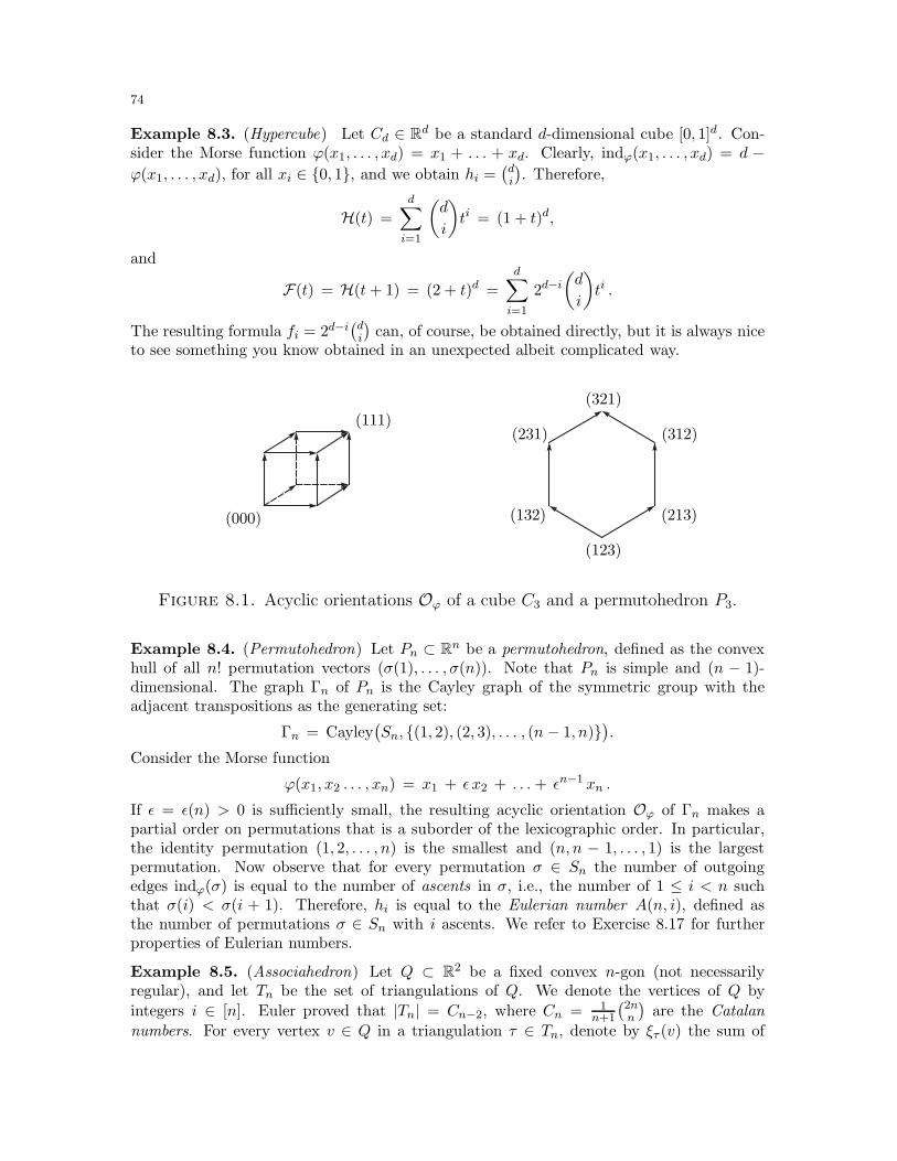
74

Example 8.3. (Hypercube) Let Cd ∈ Rd be a standard d-dimensional cube [0, 1]d. Con-sider the Morse function ϕ(x1, . . . , xd) = x1 + . . . + xd. Clearly, indϕ(x1, . . . , xd) = d −ϕ(x1, . . . , xd), for all xi ∈ 0, 1, and we obtain hi =

(di

). Therefore,

H(t) =

d∑

i=1

(d

i

)ti = (1 + t)d,

and

F(t) = H(t+ 1) = (2 + t)d =

d∑

i=1

2d−i(d

i

)ti .

The resulting formula fi = 2d−i(di

)can, of course, be obtained directly, but it is always nice

to see something you know obtained in an unexpected albeit complicated way.

(000)

(111)

(123)

(132)

(231)

(321)

(312)

(213)

Figure 8.1. Acyclic orientations Oϕ of a cube C3 and a permutohedron P3.

Example 8.4. (Permutohedron) Let Pn ⊂ Rn be a permutohedron, defined as the convexhull of all n! permutation vectors (σ(1), . . . , σ(n)). Note that Pn is simple and (n − 1)-dimensional. The graph Γn of Pn is the Cayley graph of the symmetric group with theadjacent transpositions as the generating set:

Γn = Cayley(Sn, (1, 2), (2, 3), . . . , (n − 1, n)

).

Consider the Morse function

ϕ(x1, x2 . . . , xn) = x1 + ǫ x2 + . . .+ ǫn−1 xn .

If ǫ = ǫ(n) > 0 is sufficiently small, the resulting acyclic orientation Oϕ of Γn makes apartial order on permutations that is a suborder of the lexicographic order. In particular,the identity permutation (1, 2, . . . , n) is the smallest and (n, n − 1, . . . , 1) is the largestpermutation. Now observe that for every permutation σ ∈ Sn the number of outgoingedges indϕ(σ) is equal to the number of ascents in σ, i.e., the number of 1 ≤ i < n suchthat σ(i) < σ(i + 1). Therefore, hi is equal to the Eulerian number A(n, i), defined asthe number of permutations σ ∈ Sn with i ascents. We refer to Exercise 8.17 for furtherproperties of Eulerian numbers.

Example 8.5. (Associahedron) Let Q ⊂ R2 be a fixed convex n-gon (not necessarilyregular), and let Tn be the set of triangulations of Q. We denote the vertices of Q by

integers i ∈ [n]. Euler proved that |Tn| = Cn−2, where Cn = 1n+1

(2nn

)are the Catalan

numbers. For every vertex v ∈ Q in a triangulation τ ∈ Tn, denote by ξτ (v) the sum of

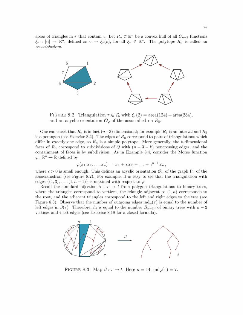
75

areas of triangles in τ that contain v. Let Rn ⊂ Rn be a convex hull of all Cn−2 functionsξτ : [n] → Rn, defined as v → ξτ (v), for all ξτ ∈ Rn. The polytope Rn is called anassociahedron.

τ

1

2

3

4

5

Figure 8.2. Triangulation τ ∈ T5 with ξτ (2) = area(124)+area(234),and an acyclic orientation Oϕ of the associahedron R5.

One can check that Rn is in fact (n−3)-dimensional; for example R4 is an interval and R5

is a pentagon (see Exercise 8.2). The edges of Rn correspond to pairs of triangulations whichdiffer in exactly one edge, so Rn is a simple polytope. More generally, the k-dimensionalfaces of Rn correspond to subdivisions of Q with (n − 3 − k) noncrossing edges, and thecontainment of faces is by subdivision. As in Example 8.4, consider the Morse functionϕ : Rn → R defined by

ϕ(x1, x2, . . . , xn) = x1 + ǫ x2 + . . .+ ǫn−1 xn ,

where ǫ > 0 is small enough. This defines an acyclic orientation Oϕ of the graph Γn of theassociahedron (see Figure 8.2). For example, it is easy to see that the triangulation withedges (1, 3), . . . , (1, n − 1) is maximal with respect to ϕ.

Recall the standard bijection β : τ → t from polygon triangulations to binary trees,where the triangles correspond to vertices, the triangle adjacent to (1, n) corresponds tothe root, and the adjacent triangles correspond to the left and right edges to the tree (seeFigure 8.3). Observe that the number of outgoing edges indϕ(τ) is equal to the number ofleft edges in β(τ). Therefore, hi is equal to the number Bn−2,i of binary trees with n − 2vertices and i left edges (see Exercise 8.18 for a closed formula).

1n

τ t

β

Figure 8.3. Map β : τ → t. Here n = 14, indϕ(τ) = 7.

76

8.3. Kalai’s simple way to tell a simple polytope from its graph. The proof ofthe Dehn-Sommerville equations shows that given an acyclic orientation Oϕ comingfrom a Morse function ϕ we can compute the f -vector of a simple polytope. It turnsout that we can obtain the whole poset of faces given just the graph Γ of the polytope.

Theorem 8.6 (Blind–Mani). Let P ∈ Rd be a simple polytope and let Γ be its graph.Then Γ determines the entire combinatorial structure of P .

In other words, given a graph Γ one can decide whether a given subset of verticesforms a k-dimensional face. The proof we present below is the celebrated proof byKalai which uses insight of Morse functions to resolve the problem.

Proof. For a subset of vertices B ⊂ V of the graph Γ to form a k-dimensional facethe induced subgraph Γ|B must be connected and k-regular. However, this is clearlynot enough. For example, a graph of 3-dimensional cube contains a cycle of length 6which is not a two-dimensional face. We will use certain acyclic orientations of Γ togive a complete characterization.

Consider an acyclic orientation O of Γ. We say that O is good if for every face F ⊂P , the corresponding graph ΓF has exactly one source. Otherwise, O is called bad.Note that in every face F , the acyclic orientation of ΓF must have at least one source.

Denote by hOi the number of vertices of index i, i.e., the number of vertices withexactly i outgoing edges and let

α(O) = hO0 + 2hO1 + 4hO2 + . . . + 2dhOd .

Finally, let β = β(P ) = f0+f1+. . .+fd be the total number of faces of all dimensions.Arguing as in the proof of the Dehn-Sommerville equations, we conclude:

• α(O) ≥ β for all O,• α(O) = β if and only if O is good.

To show this, count every face of every dimension according to the source vertices.Clearly, for a vertex v with index i, the number of such faces is at most 2i, the numberof all possible subsets of edges coming out of v. Now observe that good orientationsare exactly those where every face is counted exactly once.

This gives us a (really slow) algorithm for computing β(P ): compute α(O) for allacyclic orientations O of Γ and take the smallest value. Of course, the total numberof faces is only a tiny fraction of the information we want. What is more important isthat this approach gives a way to decide whether a given orientation is good. Havingfound one good orientation O, we can take the numbers hOi to compute the f -vector

by the formula fi =∑d

k=i hOk

(ki

). Still, this approach does not show how to start with

a good orientation of Γ, choose i edges coming out of some vertex v and compute thewhole face. Morse functions again come to the rescue.

Let B ⊂ V be a subset of vertices, a candidate for a face. We say that B is finalwith respect to an acyclic orientation O if no edge is coming out of B. We are nowready to state the main claim:

Face criterion. An induced connected k-regular subgraph H = ΓB on a set ofvertices B is a graph of a face of P if and only if there exists a good orientation Oof G, such that B is final with respect to O.

77

The ‘only if’ part can be proved as follows. Take a simple polytope P and a face Fwith the set of vertices B ⊂ V . Consider any linear function ϕ which maximizeson F . Now perturb ϕ to make it a Morse function but keep B final with respect to ϕ.This is clearly possible and gives the desired construction.

The ‘if’ part is more delicate. Let v be any source point of the graph H withrespect to O (for now we do not know if such a point is unique). Take all k edgesin H that are coming out of v. Since O is good, there exists a k-dimensional face Fwith v as its minimum. Since B is final with respect to O, we have F ⊆ B and thegraph Y = ΓF is a subgraph of H . Finally, since P is simple and F is k-dimensional,the graph Y of Γ is also k-regular.

Now compare graphs H and Y . Both are connected, k-regular, and Y ⊆ H . Thisimplies that Y = H , which proves the face criterion and the theorem.20

Remark 8.7. A couple of things are worth noting while we are on the subject. First, the

above criteria gives a ‘really slow’ algorithm for deciding if a subset is a facet. A polynomial

time algorithm was recently found in [Fri]. Second, one cannot easily use this idea to decide

whether a given graph is a graph of a simple polytope; this problem is believed to be very

difficult (see [Kaib]).

8.4. Graph connectivity via Morse functions. It is well known and easy to provethat graphs of 3-dimensional polytopes are 3-connected, but the corresponding resultfor d-dimensional polytopes is less standard. The proof again is based on Morsefunctions.

A graph is called d-connected if the removal of any d−1 vertices leaves a connectedgraph.

Theorem 8.8 (Balinski). The graph Γ of a d-dimensional polytope P is d-connected.

Proof. Let V be a set of vertices in Γ and let X = x1, . . . , xd−1 be any subset of d−1vertices. We need to prove that Γ|VrX is connected. Fix a vertex z ∈ V rX and letψ : Rd → R be a linear function which is constant on X + z:

ψ(x1) = . . . = ψ(xd−1) = ψ(z) = c ,

for some c ∈ R. The set of vertices v /∈ (X + z) is now split into two subsets:V+ = v ∈ V | ψ(v) > c and V− = v ∈ V | ψ(v) < c. There are two cases:

1) One of the sets V− or V+ is empty. Say, V− = ∅. Perturb ψ to obtain a Morsefunction ϕ : Rd → R (i.e., a function which is nonconstant on the edges of P ). Orientall edges in Γ, from a vertex with smaller to a vertex with larger value of ϕ, anddenote by w+ the maximal vertex. Now observe that for every vertex v ∈ V+ − w+

there is an edge coming out of v. Continue walking along the path of increasing edgesuntil we eventually reach the unique maximum w+. Similarly, since |X| < d, vertex zalso has an edge connecting it to V+. Therefore, all vertices in V rX are connectedto w+, which finishes the proof of this case.

20While the implication is obvious in this case, it can be viewed as a special case of a general ‘local⇒ global’ principle. In a very similar context this idea also appears in the proof of Lemmas 14.7and 35.1.

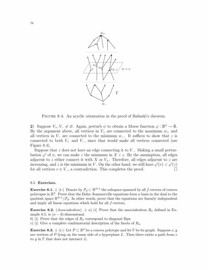
78

zx1

x2 xd−1

w+

w−

ψ = c

Γ

Figure 8.4. An acyclic orientation in the proof of Balinski’s theorem.

2) Suppose V+, V− 6= ∅. Again, perturb ψ to obtain a Morse function ϕ : Rd → R.By the argument above, all vertices in V+ are connected to the maximum w+ andall vertices in V− are connected to the minimum w−. It suffices to show that z isconnected to both V+ and V−, since that would make all vertices connected (seeFigure 8.4).

Suppose that z does not have an edge connecting it to V−. Making a small pertur-bation ϕ′ of ψ, we can make z the minimum in X + z. By the assumption, all edgesadjacent to z either connect it with X or V+. Therefore, all edges adjacent to z areincreasing, and z is the minimum in V . On the other hand, we still have ϕ′(v) < ϕ′(z)for all vertices v ∈ V−, a contradiction. This completes the proof.

8.5. Exercises.

Exercise 8.1. ♦ [1-] Denote by Fd ⊂ Rd+1 the subspace spanned by all f -vectors of convexpolytopes in Rd. Prove that the Dehn–Sommerville equations form a basis in the dual to thequotient space Rd+1/Fd. In other words, prove that the equations are linearly independentand imply all linear equations which hold for all f -vectors.

Exercise 8.2. (Associahedron) ♦ a) [1] Prove that the associahedron Rn defined in Ex-ample 8.5, is (n− 3)-dimensional.b) [1] Prove that the edges of Rn correspond to diagonal flips.c) [1] Give a complete combinatorial description of the facets of Rn.

Exercise 8.3. ♦ [1-] Let P ⊂ Rd be a convex polytope and let Γ be its graph. Suppose x, yare vertices of P lying on the same side of a hyperplane L. Then there exists a path from xto y in Γ that does not intersect L.

79

Exercise 8.4. ♦ [1+] Let P ⊂ Rd be a convex polytope with n vertices. For a vertexv ∈ P denote by Cv the infinite cone with a vertex at v, which is spanned by the edges of Pcontaining v. Prove that P is the intersection of at most n− d+ 1 cones Cv. Deduce fromhere the Balinski’s theorem (Theorem 8.8).

Exercise 8.5. Let Γ be a graph of a convex polytope P ⊂ Rd.a) [1-] Prove that if P ⊂ R3 is simplicial, then the edges of P can be colored with twocolors so that between every two vertices there are monochromatic paths of both colors.b) [1-] Find all simple polytopes P ⊂ R3 for which such a 2-coloring exists.c) [1] Generalize part a) to simplicial polytopes in Rd and d− 1 colors.

Exercise 8.6. [1] Let P ⊂ Rd be a convex polytope and let Γ be its graph. Prove thatthere is an embedding of Kd+1 into Γ, i.e., there exist d+ 1 different vertices in P every twoof which are connected by pairwise disjoint paths in Γ.

Exercise 8.7. [1] Let P ⊂ R3 be a convex polytope with even-sided faces. Prove ordisprove: the edges of P can be 2-colored so that every face has an equal number of edgesof each color.

Exercise 8.8. a) ♦ [1-] Prove that every convex polytope P ⊂ R3 has a vertex of degreeat most 5.b) [2-] Prove that every convex polytope P ⊂ R3 has two adjacent vertices whose totaldegree is at most 13.c) [2-] Prove that every convex polytope P ⊂ R3 with even-sided faces has two adjacentvertices whose total degree is at most 8.d) [1] Show that the upper bounds in part b) and c) are sharp.

Exercise 8.9. a) [1] Let P ⊂ R3 be a convex polytope and let L be the sum of edge lengthsof P . Prove that L ≥ 3diam(P ).b) [1+] Let Γ be the graph of a convex polytope P ⊂ R3 with n vertices. Prove that thediameter of Γ is at most (n− 1)/3. Show that this inequality is sharp.

Exercise 8.10. Let Γ be the graph of a simple convex polytope P ⊂ R3 with triangularand hexagonal faces.a) [1-] Prove that P has exactly four triangular faces.b) [2-] Prove that the number of hexagonal faces P is even.c) [2] Let P ⊂ R3 be a simple polytope, whose faces have 3, 6, 9, . . . sides. Prove that thenumber of faces of P is even.

Exercise 8.11. [1-] Let Q ⊂ R2 be a closed (possibly self-intersecting) polygonal curve,such that all angles are < π. Fix a Morse function, i.e., a linear function ϕ : R2 → R whichis non-constant on the edges of Q. Prove that Q is a convex polygon if and only if ϕ has aunique local maximum.

Exercise 8.12. (Neighborly polytopes) [1] Construct explicitly a convex polytope P ⊂ R4

with 6 vertices and(62

)= 15 edges. In general, we say that a polytope is neighborly if its

graph is a complete graph. For all d ≥ 4 construct a neighborly polytope in Rd with d+ 2vertices.

Exercise 8.13. [1] Let P ⊂ Rd be a convex polytope with n ≥ d+ 2 vertices. Prove thatthere exists a vertex v ∈ P and two facets, such that v /∈ F1, F2. Moreover, we can make F1

and F2 adjacent, which means that their intersection must be a (d− 2)-dimensional face.

80

Exercise 8.14. [1] Let P ⊂ Rd be a convex polytope with n ≥ d+ 2 vertices. Prove thatfor every k, 1 ≤ k ≤ d − 1, there exist a k-face and a (d − k)-dimensional face of P whichare disjoint.

Exercise 8.15. Consider all cross sections of a convex polytope P ⊂ R3 which do notcontain any vertices.a) [1-] Can all these cross sections be triangles?b) [1-] Can all these cross sections be quadrilaterals?c) [1-] Can all these cross sections be odd-sided polygons?d) [1] Suppose all vertices of P have even degree. Prove that every cross section of P is aneven-sided polygon.

Exercise 8.16. Denote by α(Γ) the length of the longest cycle in the graph Γ (cycles donot have repeated vertices).a) [1-] Find a convex polytope P with n vertices, such that the graph Γ = Γ(P ) hasα(Γ) < n.b) [1+] Construct a sequence of convex polytopes Pk with graphs Γk = Γ(Pk) on nkvertices, such that ni →∞, and α(Γk) = O(n1−ε

k ) as k →∞, for some ε > 0.

Exercise 8.17. (Eulerian numbers) ♦ In the notation of Example 8.4, let A(n, k) be thenumber of permutations σ ∈ Sn with k ascents. The integers (A0, A1, . . . , An−1) are calledEulerian numbers.a) [1-] Prove that Eulerian numbers satisfy:

A(n, k) = (n− k)A(n − 1, k − 1) + (k + 1)A(n − 1, k).

b) [1] Prove that the Eulerian numbers satisfy

Ak = n! vol(Qn,k),

where Qn,k ⊂ Rn is a convex polytope defined by the inequalities

k ≤ x1 + . . .+ xn ≤ k + 1, 0 ≤ xi ≤ 1, 1 ≤ i ≤ n.c) [1] Observe that that the Eulerian numbers satisfy

A(n, k) = n! vol(Pn,k),

where Pn,k ⊂ Rn is a union of simplices 0 ≤ xσ(1) ≤ . . . ≤ xσ(n) ≤ 1, over all σ ∈ Sn withexactly k ascents. Find an explicit piecewise-linear volume-preserving map ϕ : Qn,k → Pn,k.This gives an alternative proof of b).

Exercise 8.18. (Narayana numbers) ♦ In the notation of Example 8.5, let Bn,k be thenumber of binary trees with n vertices and k left edges. Numbers Bn,k are called Narayananumbers.a) [1-] Use induction to prove a closed formula:

Bn,k =1

n

(n

k

)(n

k + 1

).

b) [1] Use binomial identities to obtain a closed formula for the f -vector of associahedron Rn:

fi =1

n− d− 2

(n− 3

n− d− 3

)(2n− d− 4

n− d− 3

).

c) [1-] Use induction to give an alternative proof of this formula.

81

Exercise 8.19. ♦ The Birkhoff polytope Bn is defined by the following equations andinequalities:

n∑

i=1

ai,j =

n∑

j=1

ai,j = 1, and ai,j ≥ 0, for all 1 ≤ i, j ≤ n.

a) [1-] Prove that Bn has dimension (n − 1)2.b) [1] Prove that Bn has n! vertices which correspond to permutation matrices.c) [1] Prove that the edges of Bn correspond to multiplication of permutations by singlecycles. Conclude the graph of Bn has diameter two, and the vertices have degree θ

((n−1)!

).

d) [1-] Check that B3 is both neighborly (see Exercise 8.12) and simplicial, and that Bn,n ≥ 4, are neither.e) [1-] Compute vol(B3).f) [2-] Let G be a subgraph of Kn,n. We say that G is elementary if every edge of Gbelongs to some perfect matching in G. Prove that the poset of elementary subgraphsof Kn,n ordered by inclusion is isomorphic to the face lattice of Bn.g) [2-] Describe the f -vector of Bn in terms of elementary graphs.

Exercise 8.20. ♦ Define the transportation polytope Tm,n by the following equations andinequalities:

m∑

i=1

ai,j = m,n∑

j=1

ai,j = n, and ai,j ≥ 0, for all 1 ≤ i ≤ m, 1 ≤ j ≤ n.

a) [1-] Prove that Tm,n has dimension (m− 1)(n − 1).b) [2-] Prove that Tm,n is simple for all (m,n) = 1.c) [1] Show that Tn,n+1 has (n+1)n−1n! vertices. To do that, give a bijective proof betweenthese vertices of Tn,n+1 and labeled trees on n + 1 vertices, where both vertices and edgesare labeled, and use Cayley’s formula.d) [1] Find a complete description of the edges of Tn,n+1 in terms of these labeled trees.e) [1+] Use the Morse function approach to compute h1 and h2 of the simple polytope Tn,n+1.From here, obtain f2

(Tn,n+1

).

Exercise 8.21. (Klyachko lemma) [1+] Let P ⊂ R3 be a convex polytope. Fix ε > 0.Suppose on every facet F in P , there is a particle which moves clockwise along the edgesof F with the speed at least ε. Prove that at some point some two particles will collide.

Exercise 8.22. (3d-conjecture) Let P ⊂ Rd be a centrally symmetric convex polytopewith f -vector (f0, f1, . . . , fd).a) [1+] For d = 3, prove that f0 + f1 + f2 + f3 ≥ 27.b) [2+] For d = 4, prove that f0 + f1 + f2 + f3 + f4 ≥ 81.c) [∗] Prove that f0 + f1 + f2 + . . .+ fd ≥ 3d, for all d ≥ 1.

8.6. Final remarks. The generalization (♥) of Euler’s formula is due to Poincare (1897).The Dehn–Sommerville equations (Theorem 8.1) in dimensions 4 and 5 were discoveredby Dehn (1905) and generalized to all dimensions by Sommerville (1927). Note that inthe original form, the equations gave a different basis in the affine space spanned by thef -vectors of all simple polytopes in Rd (cf. Exercise 8.1). Our proof is standard and canbe found in [Brø] (see also [Barv, § Vi.6]), while a traditional proof can be found in [Gru4,§9.2]. See also [Zie1, §8.3] for the dual treatment (called shelling) of simplicial (rather than

82

simple) polytopes, as this approach is connected to further combinatorial questions andideas.

The proof of Theorem 8.6 is essentially the same as Kalai’s original argument [Kal1](see also [Zie1, §3.4]). Our proof of Balinski’s theorem (Theorem 8.8) is a variation on theoriginal proof [Bali] and the argument in [Bar3] (see also [Zie1, §3.5] and Exercise 8.4), butthe use of Morse functions allows us to avoid some unnecessary technicalities.

Eulerian numbers appear in numerous instances in enumerative combinatorics; it is oneof the two major statistics on permutations.21 We refer to [Sta3] for other appearancesof Eulerian numbers, Catalan numbers and polygon subdivisions. The associahedron isalso called the Stasheff polytope; in our definition we follow [GKZ, Chapter II.7]. Thecalculations in the examples are partly ours and partly folklore. For more on permutohedronand associahedron see [EKK, Zie1] and references therein. See also Section 14 for more ontriangulations.

Finally, let us mention that Morse functions are basic tools in Morse theory, a classical

branch of topology. We refer to [For] for a friendly treatment of the discrete case and further

references.

21This statistic is also called Eulerian. The other major statistic on Sn, by the number ofinversions in permutations, is called Mahonian, after British combinatorialist Percy MacMahon.

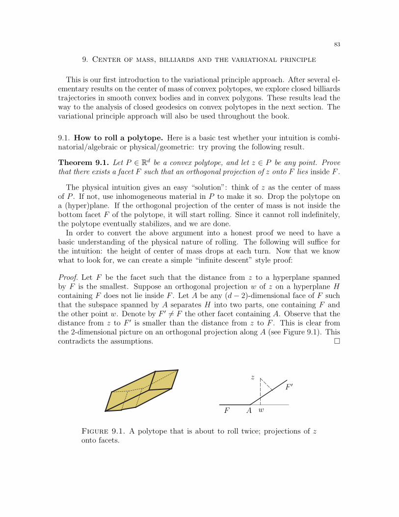
83

9. Center of mass, billiards and the variational principle

This is our first introduction to the variational principle approach. After several el-ementary results on the center of mass of convex polytopes, we explore closed billiardstrajectories in smooth convex bodies and in convex polygons. These results lead theway to the analysis of closed geodesics on convex polytopes in the next section. Thevariational principle approach will also be used throughout the book.

9.1. How to roll a polytope. Here is a basic test whether your intuition is combi-natorial/algebraic or physical/geometric: try proving the following result.

Theorem 9.1. Let P ∈ Rd be a convex polytope, and let z ∈ P be any point. Provethat there exists a facet F such that an orthogonal projection of z onto F lies inside F .

The physical intuition gives an easy “solution”: think of z as the center of massof P . If not, use inhomogeneous material in P to make it so. Drop the polytope ona (hyper)plane. If the orthogonal projection of the center of mass is not inside thebottom facet F of the polytope, it will start rolling. Since it cannot roll indefinitely,the polytope eventually stabilizes, and we are done.

In order to convert the above argument into a honest proof we need to have abasic understanding of the physical nature of rolling. The following will suffice forthe intuition: the height of center of mass drops at each turn. Now that we knowwhat to look for, we can create a simple “infinite descent” style proof:

Proof. Let F be the facet such that the distance from z to a hyperplane spannedby F is the smallest. Suppose an orthogonal projection w of z on a hyperplane Hcontaining F does not lie inside F . Let A be any (d− 2)-dimensional face of F suchthat the subspace spanned by A separates H into two parts, one containing F andthe other point w. Denote by F ′ 6= F the other facet containing A. Observe that thedistance from z to F ′ is smaller than the distance from z to F . This is clear fromthe 2-dimensional picture on an orthogonal projection along A (see Figure 9.1). Thiscontradicts the assumptions.

z

F

F ′

wA

Figure 9.1. A polytope that is about to roll twice; projections of zonto facets.

84

9.2. Meditation on the rules and the role of rolling. Let us further discussthe merits and demerits of the above “physical proof” vs. the formal proof of theadmittedly easy Theorem 9.1. Basically, the “physical proof” comes with an algorithmfor finding a desired facet F : start at any facet F0 and move repeatedly to an adjacentfacet that is closer to z, until this is no longer possible. This algorithm, of course,can be formalized, but some questions remain.

First, on the complexity of the algorithm. Clearly, not more than fd−1(P ) (the totalnumber of facets) of rolls is needed. In fact this is tight up to an additive constant22.On the other hand, the algorithm does not necessarily finds the closest facet used inthe formal proof.

Now, note that the minimum plays a special role in the proof and cannot be replacedby the maximum. The situation is strikingly different in the smooth case. We willrestrict ourselves to the dimension two case.

Let C ⊂ R2 be a smooth closed curve in the plane and let O be the origin. Through-out the section we will always assume that O /∈ C. For a point x ∈ C we say thatthe line segment (O, x) is normal if it is orthogonal to C at point x.

Proposition 9.2. Every smooth closed curve C has at least two normals from everypoint O /∈ C.

Proof. Let f(x) denote the distance from x ∈ C to the origin O. Take any (local orglobal) extremal point x (minimum or maximum) of f . Observe that (O, x) is normal,since otherwise close points on the side with angle > π/2 are at distance > |Ox|, andon the side with angle < π/2 are at distance < |Ox| (see Figure 9.2).

O

Ox

Figure 9.2. Normal points on a curve.

Note that we already used this argument in the proof of Theorem 3.3 (compareFigures 3.3 and 9.2). One can again give similar ‘physical motivation’: when C isconvex, think of it as a two-dimensional ‘die’ filled to make any interior point itscenter of mass. Place it on a line and let it roll. The (local) minima and maximacorrespond to stable and unstable equilibrium points, respectively.

Since we are really interested in discrete geometry, let us give a discrete versionof Proposition 9.2. Let Q ⊂ R2 be a polygon in the plane, possibly with self-intersections. As before, we assume that O /∈ Q. An interval (O, x), x ∈ Q, is

22Try to find an example in any fixed dimension!

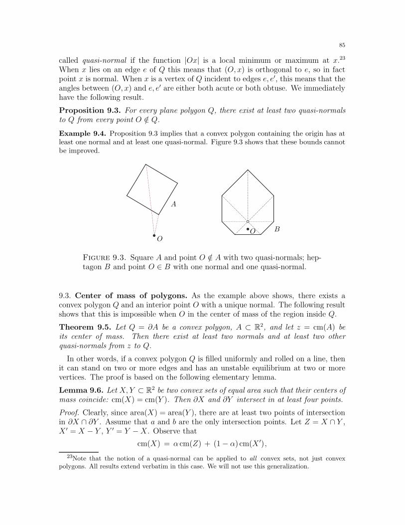
85

called quasi-normal if the function |Ox| is a local minimum or maximum at x.23

When x lies on an edge e of Q this means that (O, x) is orthogonal to e, so in factpoint x is normal. When x is a vertex of Q incident to edges e, e′, this means that theangles between (O, x) and e, e′ are either both acute or both obtuse. We immediatelyhave the following result.

Proposition 9.3. For every plane polygon Q, there exist at least two quasi-normalsto Q from every point O /∈ Q.

Example 9.4. Proposition 9.3 implies that a convex polygon containing the origin has atleast one normal and at least one quasi-normal. Figure 9.3 shows that these bounds cannotbe improved.

OO B

A

Figure 9.3. Square A and point O /∈ A with two quasi-normals; hep-tagon B and point O ∈ B with one normal and one quasi-normal.

9.3. Center of mass of polygons. As the example above shows, there exists aconvex polygon Q and an interior point O with a unique normal. The following resultshows that this is impossible when O in the center of mass of the region inside Q.

Theorem 9.5. Let Q = ∂A be a convex polygon, A ⊂ R2, and let z = cm(A) beits center of mass. Then there exist at least two normals and at least two otherquasi-normals from z to Q.

In other words, if a convex polygon Q is filled uniformly and rolled on a line, thenit can stand on two or more edges and has an unstable equilibrium at two or morevertices. The proof is based on the following elementary lemma.

Lemma 9.6. Let X, Y ⊂ R2 be two convex sets of equal area such that their centers ofmass coincide: cm(X) = cm(Y ). Then ∂X and ∂Y intersect in at least four points.

Proof. Clearly, since area(X) = area(Y ), there are at least two points of intersectionin ∂X ∩ ∂Y . Assume that a and b are the only intersection points. Let Z = X ∩ Y ,X ′ = X − Y , Y ′ = Y −X. Observe that

cm(X) = α cm(Z) + (1− α) cm(X ′),

23Note that the notion of a quasi-normal can be applied to all convex sets, not just convexpolygons. All results extend verbatim in this case. We will not use this generalization.

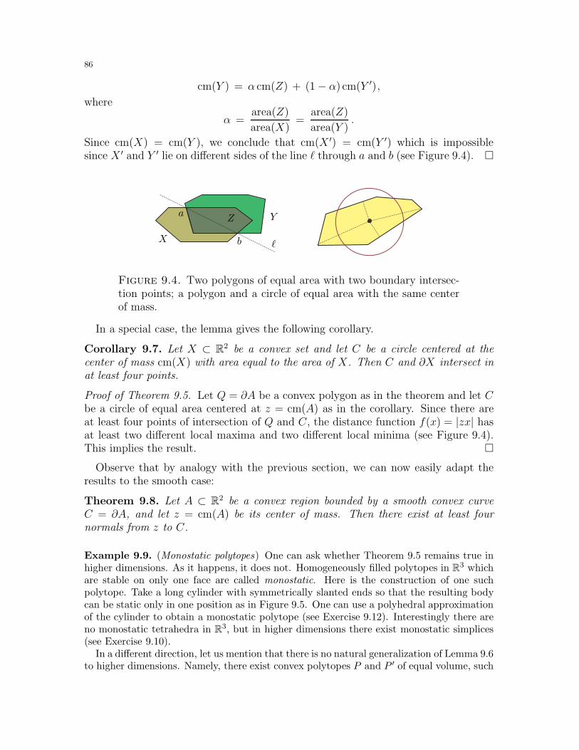
86

cm(Y ) = α cm(Z) + (1− α) cm(Y ′),

where

α =area(Z)

area(X)=

area(Z)

area(Y ).

Since cm(X) = cm(Y ), we conclude that cm(X ′) = cm(Y ′) which is impossiblesince X ′ and Y ′ lie on different sides of the line ℓ through a and b (see Figure 9.4).

Y

X

Za

b ℓ

Figure 9.4. Two polygons of equal area with two boundary intersec-tion points; a polygon and a circle of equal area with the same centerof mass.

In a special case, the lemma gives the following corollary.

Corollary 9.7. Let X ⊂ R2 be a convex set and let C be a circle centered at thecenter of mass cm(X) with area equal to the area of X. Then C and ∂X intersect inat least four points.

Proof of Theorem 9.5. Let Q = ∂A be a convex polygon as in the theorem and let Cbe a circle of equal area centered at z = cm(A) as in the corollary. Since there areat least four points of intersection of Q and C, the distance function f(x) = |zx| hasat least two different local maxima and two different local minima (see Figure 9.4).This implies the result.

Observe that by analogy with the previous section, we can now easily adapt theresults to the smooth case:

Theorem 9.8. Let A ⊂ R2 be a convex region bounded by a smooth convex curveC = ∂A, and let z = cm(A) be its center of mass. Then there exist at least fournormals from z to C.

Example 9.9. (Monostatic polytopes) One can ask whether Theorem 9.5 remains true inhigher dimensions. As it happens, it does not. Homogeneously filled polytopes in R3 whichare stable on only one face are called monostatic. Here is the construction of one suchpolytope. Take a long cylinder with symmetrically slanted ends so that the resulting bodycan be static only in one position as in Figure 9.5. One can use a polyhedral approximationof the cylinder to obtain a monostatic polytope (see Exercise 9.12). Interestingly there areno monostatic tetrahedra in R3, but in higher dimensions there exist monostatic simplices(see Exercise 9.10).

In a different direction, let us mention that there is no natural generalization of Lemma 9.6to higher dimensions. Namely, there exist convex polytopes P and P ′ of equal volume, such

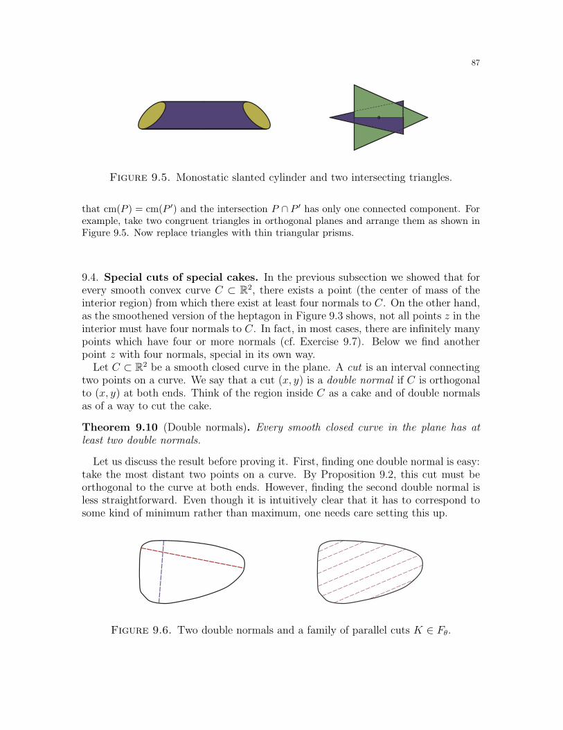
87

Figure 9.5. Monostatic slanted cylinder and two intersecting triangles.

that cm(P ) = cm(P ′) and the intersection P ∩ P ′ has only one connected component. Forexample, take two congruent triangles in orthogonal planes and arrange them as shown inFigure 9.5. Now replace triangles with thin triangular prisms.

9.4. Special cuts of special cakes. In the previous subsection we showed that forevery smooth convex curve C ⊂ R2, there exists a point (the center of mass of theinterior region) from which there exist at least four normals to C. On the other hand,as the smoothened version of the heptagon in Figure 9.3 shows, not all points z in theinterior must have four normals to C. In fact, in most cases, there are infinitely manypoints which have four or more normals (cf. Exercise 9.7). Below we find anotherpoint z with four normals, special in its own way.

Let C ⊂ R2 be a smooth closed curve in the plane. A cut is an interval connectingtwo points on a curve. We say that a cut (x, y) is a double normal if C is orthogonalto (x, y) at both ends. Think of the region inside C as a cake and of double normalsas of a way to cut the cake.

Theorem 9.10 (Double normals). Every smooth closed curve in the plane has atleast two double normals.

Let us discuss the result before proving it. First, finding one double normal is easy:take the most distant two points on a curve. By Proposition 9.2, this cut must beorthogonal to the curve at both ends. However, finding the second double normal isless straightforward. Even though it is intuitively clear that it has to correspond tosome kind of minimum rather than maximum, one needs care setting this up.

Figure 9.6. Two double normals and a family of parallel cuts K ∈ Fθ.

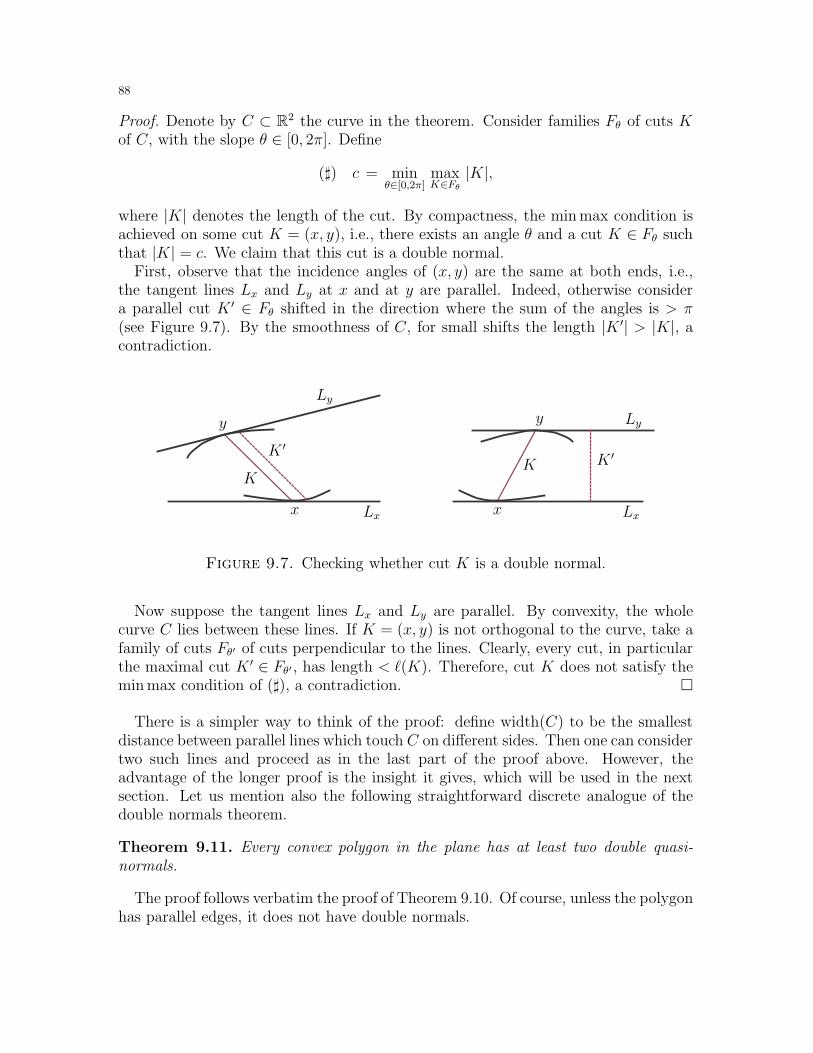
88

Proof. Denote by C ⊂ R2 the curve in the theorem. Consider families Fθ of cuts Kof C, with the slope θ ∈ [0, 2π]. Define

(♯) c = minθ∈[0,2π]

maxK∈Fθ

|K|,

where |K| denotes the length of the cut. By compactness, the min max condition isachieved on some cut K = (x, y), i.e., there exists an angle θ and a cut K ∈ Fθ suchthat |K| = c. We claim that this cut is a double normal.

First, observe that the incidence angles of (x, y) are the same at both ends, i.e.,the tangent lines Lx and Ly at x and at y are parallel. Indeed, otherwise considera parallel cut K ′ ∈ Fθ shifted in the direction where the sum of the angles is > π(see Figure 9.7). By the smoothness of C, for small shifts the length |K ′| > |K|, acontradiction.

KK

K ′K ′

LxLx

Ly

Ly

yy

xx

Figure 9.7. Checking whether cut K is a double normal.

Now suppose the tangent lines Lx and Ly are parallel. By convexity, the wholecurve C lies between these lines. If K = (x, y) is not orthogonal to the curve, take afamily of cuts Fθ′ of cuts perpendicular to the lines. Clearly, every cut, in particularthe maximal cut K ′ ∈ Fθ′ , has length < ℓ(K). Therefore, cut K does not satisfy themin max condition of (♯), a contradiction.

There is a simpler way to think of the proof: define width(C) to be the smallestdistance between parallel lines which touch C on different sides. Then one can considertwo such lines and proceed as in the last part of the proof above. However, theadvantage of the longer proof is the insight it gives, which will be used in the nextsection. Let us mention also the following straightforward discrete analogue of thedouble normals theorem.

Theorem 9.11. Every convex polygon in the plane has at least two double quasi-normals.

The proof follows verbatim the proof of Theorem 9.10. Of course, unless the polygonhas parallel edges, it does not have double normals.

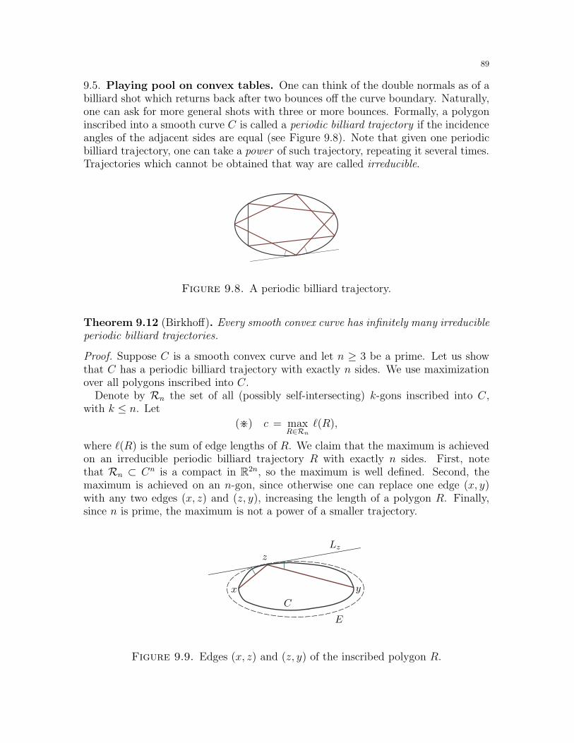
89

9.5. Playing pool on convex tables. One can think of the double normals as of abilliard shot which returns back after two bounces off the curve boundary. Naturally,one can ask for more general shots with three or more bounces. Formally, a polygoninscribed into a smooth curve C is called a periodic billiard trajectory if the incidenceangles of the adjacent sides are equal (see Figure 9.8). Note that given one periodicbilliard trajectory, one can take a power of such trajectory, repeating it several times.Trajectories which cannot be obtained that way are called irreducible.

Figure 9.8. A periodic billiard trajectory.

Theorem 9.12 (Birkhoff). Every smooth convex curve has infinitely many irreducibleperiodic billiard trajectories.

Proof. Suppose C is a smooth convex curve and let n ≥ 3 be a prime. Let us showthat C has a periodic billiard trajectory with exactly n sides. We use maximizationover all polygons inscribed into C.

Denote by Rn the set of all (possibly self-intersecting) k-gons inscribed into C,with k ≤ n. Let

(>) c = maxR∈Rn

ℓ(R),

where ℓ(R) is the sum of edge lengths of R. We claim that the maximum is achievedon an irreducible periodic billiard trajectory R with exactly n sides. First, notethat Rn ⊂ Cn is a compact in R2n, so the maximum is well defined. Second, themaximum is achieved on an n-gon, since otherwise one can replace one edge (x, y)with any two edges (x, z) and (z, y), increasing the length of a polygon R. Finally,since n is prime, the maximum is not a power of a smaller trajectory.

x y

z

E

C

Lz

Figure 9.9. Edges (x, z) and (z, y) of the inscribed polygon R.

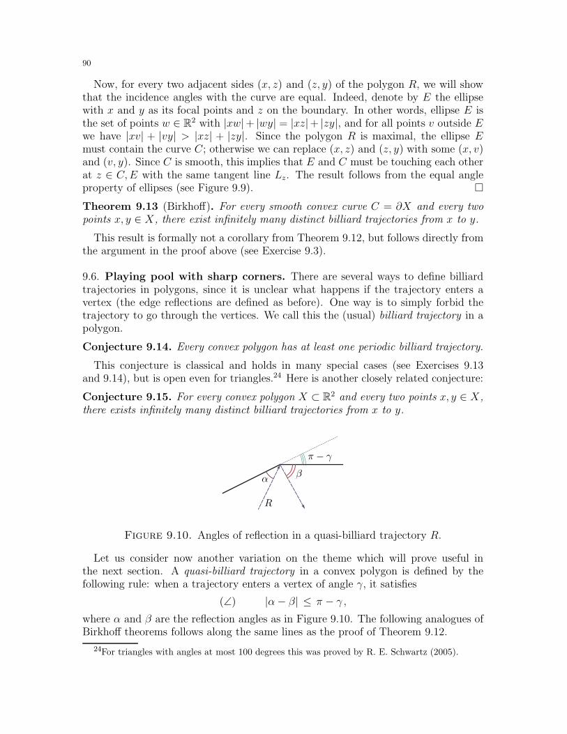
90

Now, for every two adjacent sides (x, z) and (z, y) of the polygon R, we will showthat the incidence angles with the curve are equal. Indeed, denote by E the ellipsewith x and y as its focal points and z on the boundary. In other words, ellipse E isthe set of points w ∈ R2 with |xw|+ |wy| = |xz|+ |zy|, and for all points v outside Ewe have |xv| + |vy| > |xz| + |zy|. Since the polygon R is maximal, the ellipse Emust contain the curve C; otherwise we can replace (x, z) and (z, y) with some (x, v)and (v, y). Since C is smooth, this implies that E and C must be touching each otherat z ∈ C,E with the same tangent line Lz. The result follows from the equal angleproperty of ellipses (see Figure 9.9).

Theorem 9.13 (Birkhoff). For every smooth convex curve C = ∂X and every twopoints x, y ∈ X, there exist infinitely many distinct billiard trajectories from x to y.

This result is formally not a corollary from Theorem 9.12, but follows directly fromthe argument in the proof above (see Exercise 9.3).

9.6. Playing pool with sharp corners. There are several ways to define billiardtrajectories in polygons, since it is unclear what happens if the trajectory enters avertex (the edge reflections are defined as before). One way is to simply forbid thetrajectory to go through the vertices. We call this the (usual) billiard trajectory in apolygon.

Conjecture 9.14. Every convex polygon has at least one periodic billiard trajectory.

This conjecture is classical and holds in many special cases (see Exercises 9.13and 9.14), but is open even for triangles.24 Here is another closely related conjecture:

Conjecture 9.15. For every convex polygon X ⊂ R2 and every two points x, y ∈ X,there exists infinitely many distinct billiard trajectories from x to y.

R

α β

π − γ

Figure 9.10. Angles of reflection in a quasi-billiard trajectory R.

Let us consider now another variation on the theme which will prove useful inthe next section. A quasi-billiard trajectory in a convex polygon is defined by thefollowing rule: when a trajectory enters a vertex of angle γ, it satisfies

(∠) |α− β| ≤ π − γ ,where α and β are the reflection angles as in Figure 9.10. The following analogues ofBirkhoff theorems follows along the same lines as the proof of Theorem 9.12.

24For triangles with angles at most 100 degrees this was proved by R. E. Schwartz (2005).

91

Theorem 9.16. For every convex polygon Q ⊂ R2, there exists a periodic quasi-billiard trajectory inscribed into Q with exactly n sides, for every n ≥ 3.

Theorem 9.17. For every convex polygon Q = ∂A, A ⊂ R2, and every two pointsx, y ∈ A, there exist infinitely many quasi-billiard trajectories from x to y.

Note that the Birkhoff maximization construction when applied to polygons cannever produce the usual billiard trajectories since the maximum will always be achievedat vertices. In other words, both theorems can be restated as existence results of ver-tex sequences which satisfy angle conditions as in (∠).

9.7. Exercises.

Exercise 9.1. [1-] a) Let Q ⊂ R2 be a closed polygon and let e be the longest edge. Provethat there exists a vertex v ∈ Q which projects onto e.b) [1-] Deduce part a) from the proof of Theorem 9.11.c) [1] Find a convex polytope P ⊂ R3 such that for every face F and vertex v of P , v /∈ F ,vertex v projects outside of F .

Exercise 9.2. a) [1-] Prove that every smooth convex curve C ⊂ R2 has an inscribedtriangle ∆ = (xyz), such that a line tangent to C at each of these points is parallel to theopposite edge of ∆. For example, a line tangent to C at x must be parallel to (yz).b) [1-] Show that every convex polygon Q ⊂ R2 has three vertices which form a triangle ∆,such that the line through either vertex of ∆ parallel to the opposite edge is supporting Q.c) [1] Generalize a) and b) to higher dimensions.

Exercise 9.3. ♦ a) [1-] Prove Theorem 9.13.b) [1] Give a direct proof of Theorem 9.16.c) [1] Give a direct proof of Theorem 9.17.d) [1] Deduce Theorem 9.12 from Theorem 9.16 by a limit argument.d) [1] Deduce Theorem 9.16 from Theorem 9.12 by a limit argument.

Exercise 9.4. Prove or disprove:a) [1-] Every smooth simple closed curve in R3 has a plane which touches it at three ormore points.b) [1-] Every simple space polygon Q ⊂ R3 has a plane L which contains three or morevertices of C, such that all edges adjacent to these vertices either lie on L or on the sameside of L.

Exercise 9.5. Let X ⊂ R2 be a convex set. We say that a point z ⊂ X is central if everychord through z is divided by z inside X with a ratio at most 2 : 1.a) [1-] Prove that the center of mass cm(X) is central.b) [1] Let ∆ be a triangle inscribed into X with maximal area. Prove that cm(∆) is central.

Exercise 9.6. [2-] Let Q = ∂A be a convex polygon, A ⊂ R2, and let z ∈ A be an interiorpoint. A triple of quasi-normals from z onto Q is called a tripod at z if they form an angleof 2π/3 with each other (see Figure 9.11). Prove that every convex polygon has a tripod atsome interior point.

Exercise 9.7. a) [1] Let Q = ∂A, A ⊂ R2, be a convex polygon. Denote by x = cm(Q)the center of mass of the curve with the uniform weights. Prove that there exist at leastfour quasi-normals from x onto Q.

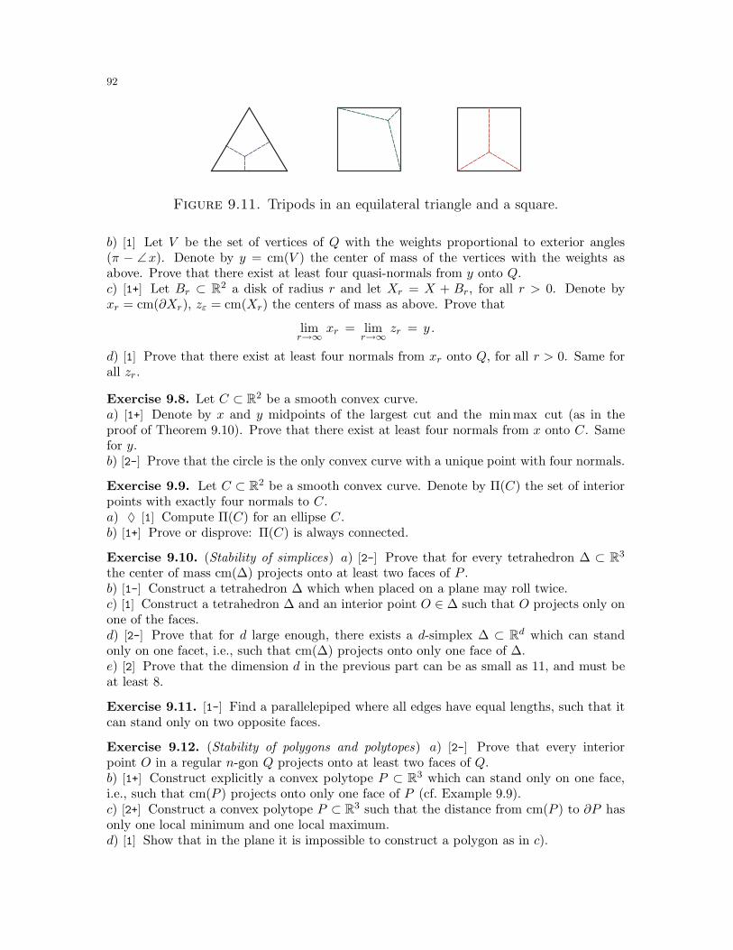
92

Figure 9.11. Tripods in an equilateral triangle and a square.

b) [1] Let V be the set of vertices of Q with the weights proportional to exterior angles(π − ∠x). Denote by y = cm(V ) the center of mass of the vertices with the weights asabove. Prove that there exist at least four quasi-normals from y onto Q.c) [1+] Let Br ⊂ R2 a disk of radius r and let Xr = X + Br, for all r > 0. Denote byxr = cm(∂Xr), zε = cm(Xr) the centers of mass as above. Prove that

limr→∞

xr = limr→∞

zr = y.

d) [1] Prove that there exist at least four normals from xr onto Q, for all r > 0. Same forall zr.

Exercise 9.8. Let C ⊂ R2 be a smooth convex curve.a) [1+] Denote by x and y midpoints of the largest cut and the min max cut (as in theproof of Theorem 9.10). Prove that there exist at least four normals from x onto C. Samefor y.b) [2-] Prove that the circle is the only convex curve with a unique point with four normals.

Exercise 9.9. Let C ⊂ R2 be a smooth convex curve. Denote by Π(C) the set of interiorpoints with exactly four normals to C.a) ♦ [1] Compute Π(C) for an ellipse C.b) [1+] Prove or disprove: Π(C) is always connected.

Exercise 9.10. (Stability of simplices) a) [2-] Prove that for every tetrahedron ∆ ⊂ R3

the center of mass cm(∆) projects onto at least two faces of P .b) [1-] Construct a tetrahedron ∆ which when placed on a plane may roll twice.c) [1] Construct a tetrahedron ∆ and an interior point O ∈ ∆ such that O projects only onone of the faces.d) [2-] Prove that for d large enough, there exists a d-simplex ∆ ⊂ Rd which can standonly on one facet, i.e., such that cm(∆) projects onto only one face of ∆.e) [2] Prove that the dimension d in the previous part can be as small as 11, and must beat least 8.

Exercise 9.11. [1-] Find a parallelepiped where all edges have equal lengths, such that itcan stand only on two opposite faces.

Exercise 9.12. (Stability of polygons and polytopes) a) [2-] Prove that every interiorpoint O in a regular n-gon Q projects onto at least two faces of Q.b) [1+] Construct explicitly a convex polytope P ⊂ R3 which can stand only on one face,i.e., such that cm(P ) projects onto only one face of P (cf. Example 9.9).c) [2+] Construct a convex polytope P ⊂ R3 such that the distance from cm(P ) to ∂P hasonly one local minimum and one local maximum.d) [1] Show that in the plane it is impossible to construct a polygon as in c).

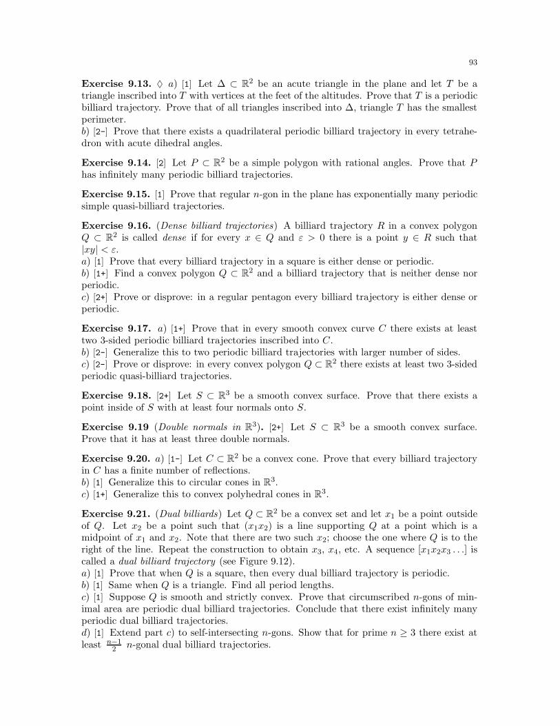
93

Exercise 9.13. ♦ a) [1] Let ∆ ⊂ R2 be an acute triangle in the plane and let T be atriangle inscribed into T with vertices at the feet of the altitudes. Prove that T is a periodicbilliard trajectory. Prove that of all triangles inscribed into ∆, triangle T has the smallestperimeter.b) [2-] Prove that there exists a quadrilateral periodic billiard trajectory in every tetrahe-dron with acute dihedral angles.

Exercise 9.14. [2] Let P ⊂ R2 be a simple polygon with rational angles. Prove that Phas infinitely many periodic billiard trajectories.

Exercise 9.15. [1] Prove that regular n-gon in the plane has exponentially many periodicsimple quasi-billiard trajectories.

Exercise 9.16. (Dense billiard trajectories) A billiard trajectory R in a convex polygonQ ⊂ R2 is called dense if for every x ∈ Q and ε > 0 there is a point y ∈ R such that|xy| < ε.a) [1] Prove that every billiard trajectory in a square is either dense or periodic.b) [1+] Find a convex polygon Q ⊂ R2 and a billiard trajectory that is neither dense norperiodic.c) [2+] Prove or disprove: in a regular pentagon every billiard trajectory is either dense orperiodic.

Exercise 9.17. a) [1+] Prove that in every smooth convex curve C there exists at leasttwo 3-sided periodic billiard trajectories inscribed into C.b) [2-] Generalize this to two periodic billiard trajectories with larger number of sides.c) [2-] Prove or disprove: in every convex polygon Q ⊂ R2 there exists at least two 3-sidedperiodic quasi-billiard trajectories.

Exercise 9.18. [2+] Let S ⊂ R3 be a smooth convex surface. Prove that there exists apoint inside of S with at least four normals onto S.

Exercise 9.19 (Double normals in R3). [2+] Let S ⊂ R3 be a smooth convex surface.Prove that it has at least three double normals.

Exercise 9.20. a) [1-] Let C ⊂ R2 be a convex cone. Prove that every billiard trajectoryin C has a finite number of reflections.b) [1] Generalize this to circular cones in R3.c) [1+] Generalize this to convex polyhedral cones in R3.

Exercise 9.21. (Dual billiards) Let Q ⊂ R2 be a convex set and let x1 be a point outsideof Q. Let x2 be a point such that (x1x2) is a line supporting Q at a point which is amidpoint of x1 and x2. Note that there are two such x2; choose the one where Q is to theright of the line. Repeat the construction to obtain x3, x4, etc. A sequence [x1x2x3 . . .] iscalled a dual billiard trajectory (see Figure 9.12).a) [1] Prove that when Q is a square, then every dual billiard trajectory is periodic.b) [1] Same when Q is a triangle. Find all period lengths.c) [1] Suppose Q is smooth and strictly convex. Prove that circumscribed n-gons of min-imal area are periodic dual billiard trajectories. Conclude that there exist infinitely manyperiodic dual billiard trajectories.d) [1] Extend part c) to self-intersecting n-gons. Show that for prime n ≥ 3 there exist atleast n−1

2 n-gonal dual billiard trajectories.

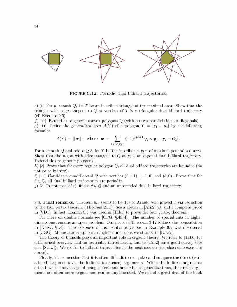
94

Figure 9.12. Periodic dual billiard trajectories.

e) [1] For a smooth Q, let T be an inscribed triangle of the maximal area. Show that thetriangle with edges tangent to Q at vertices of T is a triangular dual billiard trajectory(cf. Exercise 9.5).f) [1-] Extend e) to generic convex polygons Q (with no two parallel sides or diagonals).g) [1+] Define the generalized area A(Y ) of a polygon Y = [y1 . . . yn] by the followingformula:

A(Y ) = ‖w‖, where w =∑

1≤i<j≤n(−1)j+i+1

y i × y j , y i =−−→Oyi .

For a smooth Q and odd n ≥ 3, let Y be the inscribed n-gon of maximal generalized area.Show that the n-gon with edges tangent to Q at yi is an n-gonal dual billiard trajectory.Extend this to generic polygons.h) [2] Prove that for every regular polygon Q, all dual billiard trajectories are bounded (donot go to infinity).i) [1+] Consider a quadrilateral Q with vertices (0,±1), (−1, 0) and (θ, 0). Prove that forθ ∈ Q, all dual billiard trajectories are periodic.j) [2] In notation of i), find a θ /∈ Q and an unbounded dual billiard trajectory.

9.8. Final remarks. Theorem 9.5 seems to be due to Arnold who proved it via reductionto the four vertex theorem (Theorem 21.1). See a sketch in [Arn2, §3] and a complete proofin [VD1]. In fact, Lemma 9.6 was used in [Tab1] to prove the four vertex theorem.

For more on double normals see [CFG, §A3, 4]. The number of special cuts in higherdimensions remains an open problem. Our proof of Theorem 9.12 follows the presentationin [KleW, §1.4]. The existence of monostatic polytopes in Example 9.9 was discoveredin [CGG]. Monostatic simplices in higher dimensions we studied in [Daw2].

The theory of billiards plays an important role in ergodic theory. We refer to [Tab6] fora historical overview and an accessible introduction, and to [Tab2] for a good survey (seealso [Schw]). We return to billiard trajectories in the next section (see also some exercisesabove).

Finally, let us mention that it is often difficult to recognize and compare the direct (vari-ational) arguments vs. the indirect (existence) arguments. While the indirect argumentsoften have the advantage of being concise and amenable to generalizations, the direct argu-ments are often more elegant and can be implemented. We spend a great deal of the book

95

discussing both methods. For now, let us leave you with a few words of wisdom by SunTzu [Sun]:

iV.5. In all fighting, the direct method may be used for joining battle, butindirect methods will be needed in order to secure victory.V.10. In battle, there are not more than two methods of attack – the directand the indirect; yet these two in combination give rise to an endless series ofmaneuvers.V.11. The direct and the indirect lead on to each other in turn. It is like mov-ing in a circle – you never come to an end. Who can exhaust the possibilitiesof their combination?

These quotes are especially relevant to the proofs in Sections 35–37.

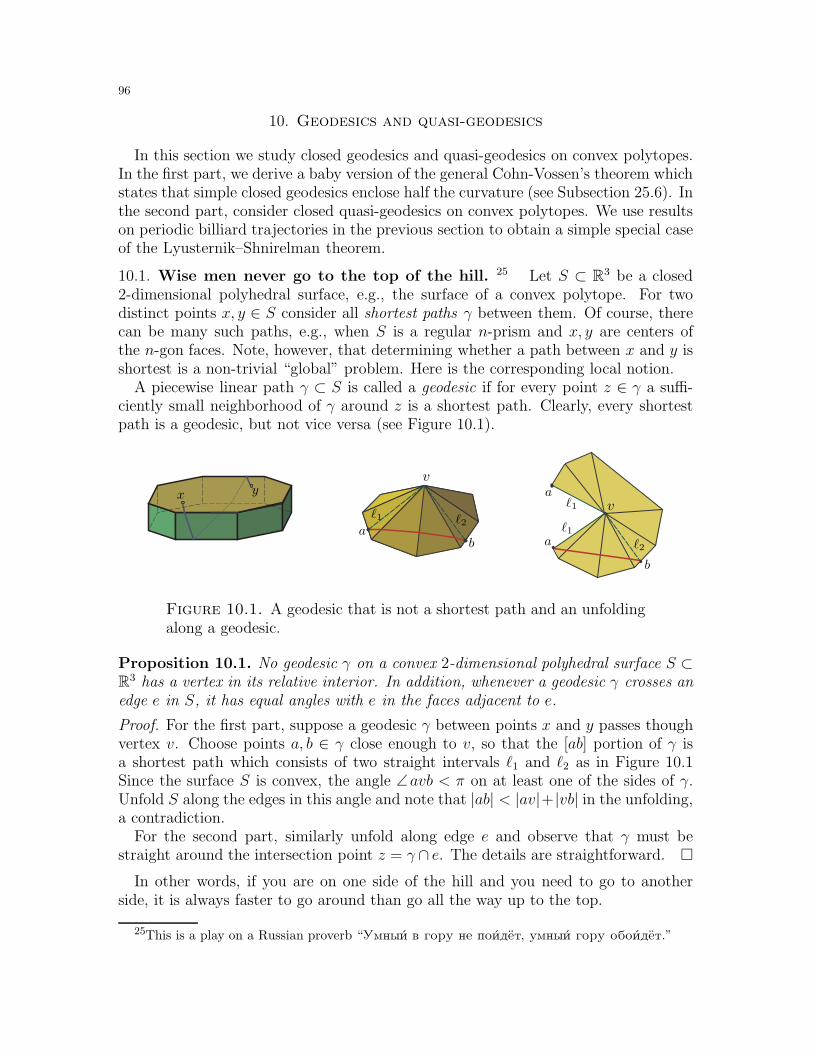
96

10. Geodesics and quasi-geodesics

In this section we study closed geodesics and quasi-geodesics on convex polytopes.In the first part, we derive a baby version of the general Cohn-Vossen’s theorem whichstates that simple closed geodesics enclose half the curvature (see Subsection 25.6). Inthe second part, consider closed quasi-geodesics on convex polytopes. We use resultson periodic billiard trajectories in the previous section to obtain a simple special caseof the Lyusternik–Shnirelman theorem.

10.1. Wise men never go to the top of the hill. 25 Let S ⊂ R3 be a closed2-dimensional polyhedral surface, e.g., the surface of a convex polytope. For twodistinct points x, y ∈ S consider all shortest paths γ between them. Of course, therecan be many such paths, e.g., when S is a regular n-prism and x, y are centers ofthe n-gon faces. Note, however, that determining whether a path between x and y isshortest is a non-trivial “global” problem. Here is the corresponding local notion.

A piecewise linear path γ ⊂ S is called a geodesic if for every point z ∈ γ a suffi-ciently small neighborhood of γ around z is a shortest path. Clearly, every shortestpath is a geodesic, but not vice versa (see Figure 10.1).

v

vx y a

aa

b

bℓ1

ℓ1ℓ1

ℓ2

ℓ2

Figure 10.1. A geodesic that is not a shortest path and an unfoldingalong a geodesic.

Proposition 10.1. No geodesic γ on a convex 2-dimensional polyhedral surface S ⊂R3 has a vertex in its relative interior. In addition, whenever a geodesic γ crosses anedge e in S, it has equal angles with e in the faces adjacent to e.

Proof. For the first part, suppose a geodesic γ between points x and y passes thoughvertex v. Choose points a, b ∈ γ close enough to v, so that the [ab] portion of γ isa shortest path which consists of two straight intervals ℓ1 and ℓ2 as in Figure 10.1Since the surface S is convex, the angle ∠avb < π on at least one of the sides of γ.Unfold S along the edges in this angle and note that |ab| < |av|+|vb| in the unfolding,a contradiction.

For the second part, similarly unfold along edge e and observe that γ must bestraight around the intersection point z = γ ∩ e. The details are straightforward.

In other words, if you are on one side of the hill and you need to go to anotherside, it is always faster to go around than go all the way up to the top.

25This is a play on a Russian proverb “Umnyi v goru ne poidet, umnyi goru oboidet.”

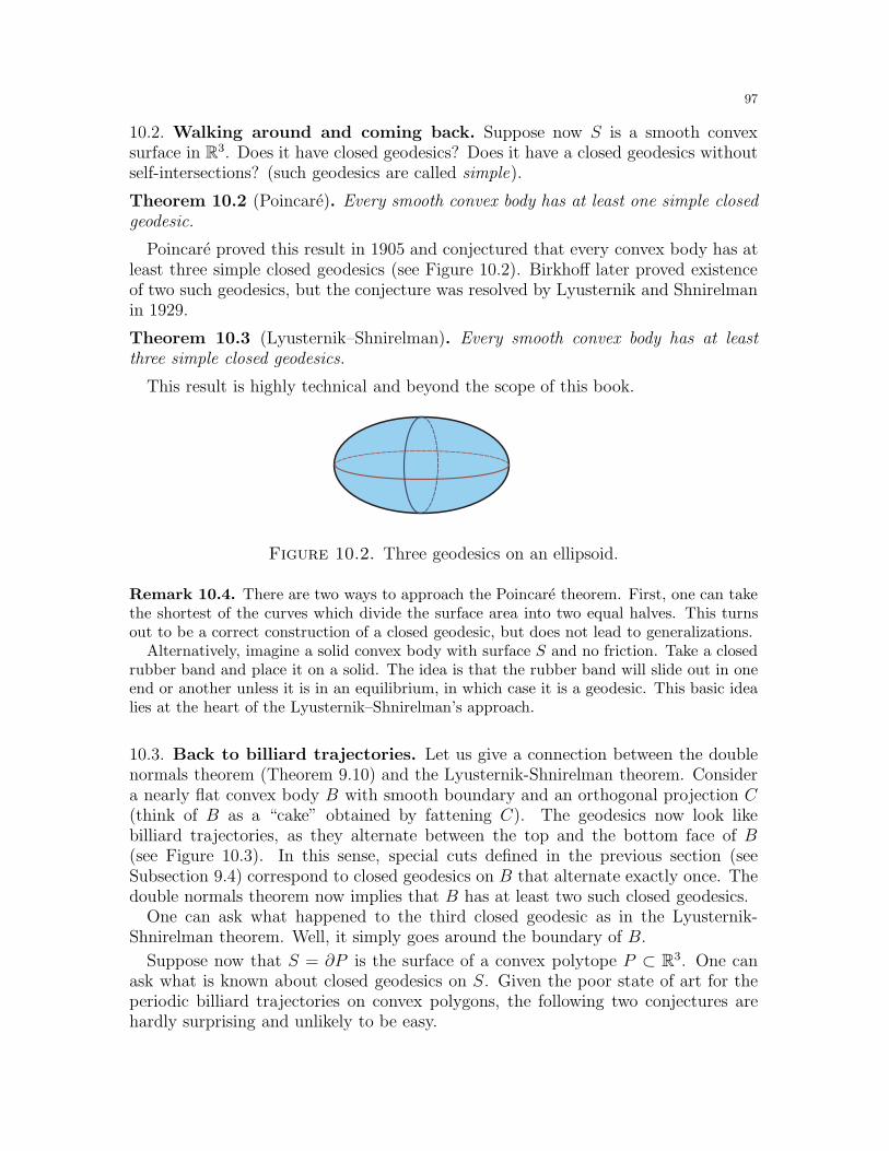
97

10.2. Walking around and coming back. Suppose now S is a smooth convexsurface in R3. Does it have closed geodesics? Does it have a closed geodesics withoutself-intersections? (such geodesics are called simple).

Theorem 10.2 (Poincare). Every smooth convex body has at least one simple closedgeodesic.

Poincare proved this result in 1905 and conjectured that every convex body has atleast three simple closed geodesics (see Figure 10.2). Birkhoff later proved existenceof two such geodesics, but the conjecture was resolved by Lyusternik and Shnirelmanin 1929.

Theorem 10.3 (Lyusternik–Shnirelman). Every smooth convex body has at leastthree simple closed geodesics.

This result is highly technical and beyond the scope of this book.

Figure 10.2. Three geodesics on an ellipsoid.

Remark 10.4. There are two ways to approach the Poincare theorem. First, one can takethe shortest of the curves which divide the surface area into two equal halves. This turnsout to be a correct construction of a closed geodesic, but does not lead to generalizations.

Alternatively, imagine a solid convex body with surface S and no friction. Take a closedrubber band and place it on a solid. The idea is that the rubber band will slide out in oneend or another unless it is in an equilibrium, in which case it is a geodesic. This basic idealies at the heart of the Lyusternik–Shnirelman’s approach.

10.3. Back to billiard trajectories. Let us give a connection between the doublenormals theorem (Theorem 9.10) and the Lyusternik-Shnirelman theorem. Considera nearly flat convex body B with smooth boundary and an orthogonal projection C(think of B as a “cake” obtained by fattening C). The geodesics now look likebilliard trajectories, as they alternate between the top and the bottom face of B(see Figure 10.3). In this sense, special cuts defined in the previous section (seeSubsection 9.4) correspond to closed geodesics on B that alternate exactly once. Thedouble normals theorem now implies that B has at least two such closed geodesics.

One can ask what happened to the third closed geodesic as in the Lyusternik-Shnirelman theorem. Well, it simply goes around the boundary of B.

Suppose now that S = ∂P is the surface of a convex polytope P ⊂ R3. One canask what is known about closed geodesics on S. Given the poor state of art for theperiodic billiard trajectories on convex polygons, the following two conjectures arehardly surprising and unlikely to be easy.

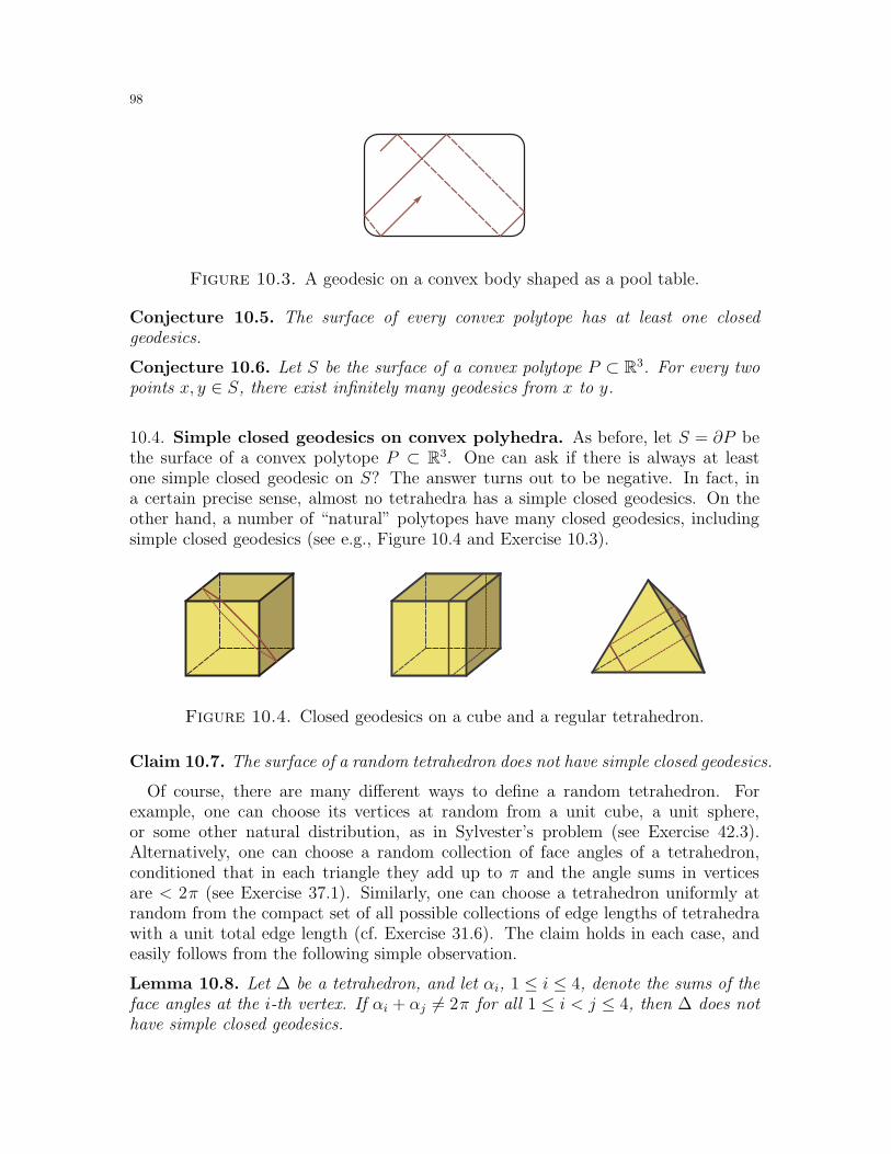
98

Figure 10.3. A geodesic on a convex body shaped as a pool table.

Conjecture 10.5. The surface of every convex polytope has at least one closedgeodesics.

Conjecture 10.6. Let S be the surface of a convex polytope P ⊂ R3. For every twopoints x, y ∈ S, there exist infinitely many geodesics from x to y.

10.4. Simple closed geodesics on convex polyhedra. As before, let S = ∂P bethe surface of a convex polytope P ⊂ R3. One can ask if there is always at leastone simple closed geodesic on S? The answer turns out to be negative. In fact, ina certain precise sense, almost no tetrahedra has a simple closed geodesics. On theother hand, a number of “natural” polytopes have many closed geodesics, includingsimple closed geodesics (see e.g., Figure 10.4 and Exercise 10.3).

Figure 10.4. Closed geodesics on a cube and a regular tetrahedron.

Claim 10.7. The surface of a random tetrahedron does not have simple closed geodesics.

Of course, there are many different ways to define a random tetrahedron. Forexample, one can choose its vertices at random from a unit cube, a unit sphere,or some other natural distribution, as in Sylvester’s problem (see Exercise 42.3).Alternatively, one can choose a random collection of face angles of a tetrahedron,conditioned that in each triangle they add up to π and the angle sums in verticesare < 2π (see Exercise 37.1). Similarly, one can choose a tetrahedron uniformly atrandom from the compact set of all possible collections of edge lengths of tetrahedrawith a unit total edge length (cf. Exercise 31.6). The claim holds in each case, andeasily follows from the following simple observation.

Lemma 10.8. Let ∆ be a tetrahedron, and let αi, 1 ≤ i ≤ 4, denote the sums of theface angles at the i-th vertex. If αi + αj 6= 2π for all 1 ≤ i < j ≤ 4, then ∆ does nothave simple closed geodesics.

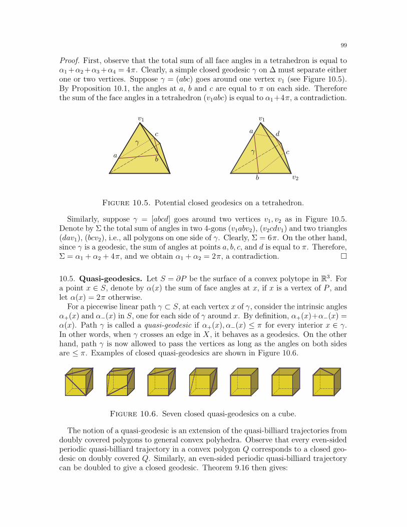
99

Proof. First, observe that the total sum of all face angles in a tetrahedron is equal toα1 +α2 +α3 +α4 = 4π. Clearly, a simple closed geodesic γ on ∆ must separate eitherone or two vertices. Suppose γ = (abc) goes around one vertex v1 (see Figure 10.5).By Proposition 10.1, the angles at a, b and c are equal to π on each side. Thereforethe sum of the face angles in a tetrahedron (v1abc) is equal to α1+4π, a contradiction.

v1v1

v2

da

a

b

bc

c

γ

γ

Figure 10.5. Potential closed geodesics on a tetrahedron.

Similarly, suppose γ = [abcd] goes around two vertices v1, v2 as in Figure 10.5.Denote by Σ the total sum of angles in two 4-gons (v1abv2), (v2cdv1) and two triangles(dav1), (bcv2), i.e., all polygons on one side of γ. Clearly, Σ = 6π. On the other hand,since γ is a geodesic, the sum of angles at points a, b, c, and d is equal to π. Therefore,Σ = α1 + α2 + 4π, and we obtain α1 + α2 = 2π, a contradiction.

10.5. Quasi-geodesics. Let S = ∂P be the surface of a convex polytope in R3. Fora point x ∈ S, denote by α(x) the sum of face angles at x, if x is a vertex of P , andlet α(x) = 2π otherwise.

For a piecewise linear path γ ⊂ S, at each vertex x of γ, consider the intrinsic anglesα+(x) and α−(x) in S, one for each side of γ around x. By definition, α+(x)+α−(x) =α(x). Path γ is called a quasi-geodesic if α+(x), α−(x) ≤ π for every interior x ∈ γ.In other words, when γ crosses an edge in X, it behaves as a geodesics. On the otherhand, path γ is now allowed to pass the vertices as long as the angles on both sidesare ≤ π. Examples of closed quasi-geodesics are shown in Figure 10.6.

Figure 10.6. Seven closed quasi-geodesics on a cube.

The notion of a quasi-geodesic is an extension of the quasi-billiard trajectories fromdoubly covered polygons to general convex polyhedra. Observe that every even-sidedperiodic quasi-billiard trajectory in a convex polygon Q corresponds to a closed geo-desic on doubly covered Q. Similarly, an even-sided periodic quasi-billiard trajectorycan be doubled to give a closed geodesic. Theorem 9.16 then gives:

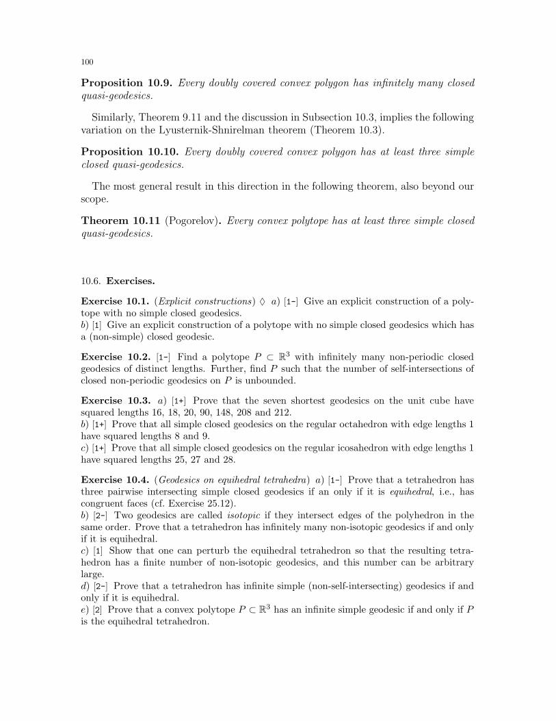
100

Proposition 10.9. Every doubly covered convex polygon has infinitely many closedquasi-geodesics.

Similarly, Theorem 9.11 and the discussion in Subsection 10.3, implies the followingvariation on the Lyusternik-Shnirelman theorem (Theorem 10.3).

Proposition 10.10. Every doubly covered convex polygon has at least three simpleclosed quasi-geodesics.

The most general result in this direction in the following theorem, also beyond ourscope.

Theorem 10.11 (Pogorelov). Every convex polytope has at least three simple closedquasi-geodesics.

10.6. Exercises.

Exercise 10.1. (Explicit constructions) ♦ a) [1-] Give an explicit construction of a poly-tope with no simple closed geodesics.b) [1] Give an explicit construction of a polytope with no simple closed geodesics which hasa (non-simple) closed geodesic.

Exercise 10.2. [1-] Find a polytope P ⊂ R3 with infinitely many non-periodic closedgeodesics of distinct lengths. Further, find P such that the number of self-intersections ofclosed non-periodic geodesics on P is unbounded.

Exercise 10.3. a) [1+] Prove that the seven shortest geodesics on the unit cube havesquared lengths 16, 18, 20, 90, 148, 208 and 212.b) [1+] Prove that all simple closed geodesics on the regular octahedron with edge lengths 1have squared lengths 8 and 9.c) [1+] Prove that all simple closed geodesics on the regular icosahedron with edge lengths 1have squared lengths 25, 27 and 28.

Exercise 10.4. (Geodesics on equihedral tetrahedra) a) [1-] Prove that a tetrahedron hasthree pairwise intersecting simple closed geodesics if an only if it is equihedral, i.e., hascongruent faces (cf. Exercise 25.12).b) [2-] Two geodesics are called isotopic if they intersect edges of the polyhedron in thesame order. Prove that a tetrahedron has infinitely many non-isotopic geodesics if and onlyif it is equihedral.c) [1] Show that one can perturb the equihedral tetrahedron so that the resulting tetra-hedron has a finite number of non-isotopic geodesics, and this number can be arbitrarylarge.d) [2-] Prove that a tetrahedron has infinite simple (non-self-intersecting) geodesics if andonly if it is equihedral.e) [2] Prove that a convex polytope P ⊂ R3 has an infinite simple geodesic if and only if Pis the equihedral tetrahedron.

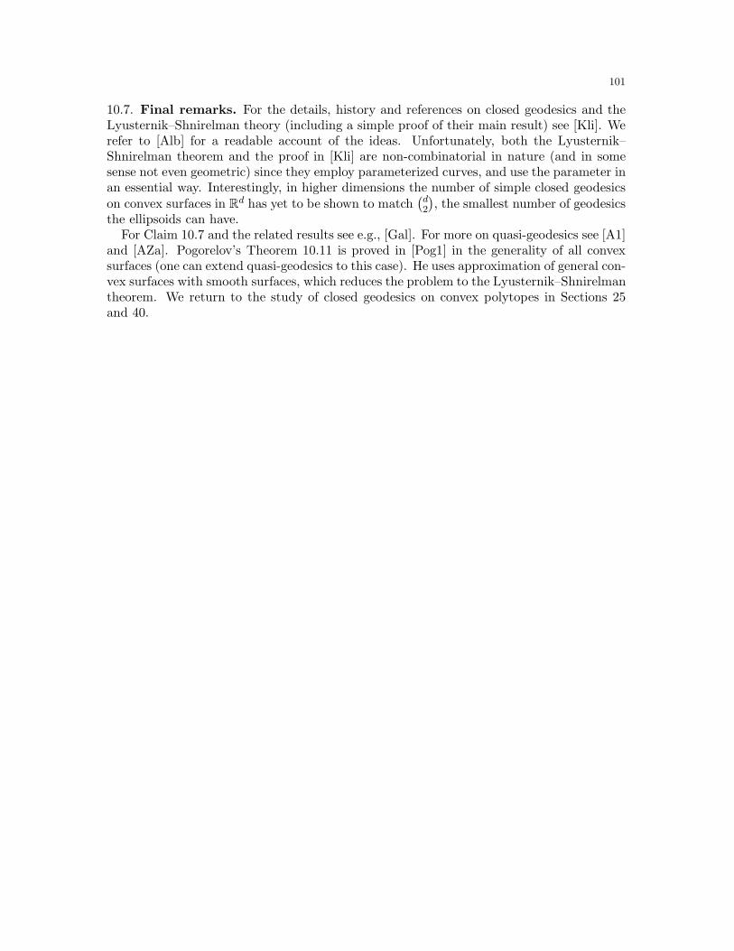
101

10.7. Final remarks. For the details, history and references on closed geodesics and theLyusternik–Shnirelman theory (including a simple proof of their main result) see [Kli]. Werefer to [Alb] for a readable account of the ideas. Unfortunately, both the Lyusternik–Shnirelman theorem and the proof in [Kli] are non-combinatorial in nature (and in somesense not even geometric) since they employ parameterized curves, and use the parameter inan essential way. Interestingly, in higher dimensions the number of simple closed geodesicson convex surfaces in Rd has yet to be shown to match

(d2

), the smallest number of geodesics

the ellipsoids can have.For Claim 10.7 and the related results see e.g., [Gal]. For more on quasi-geodesics see [A1]

and [AZa]. Pogorelov’s Theorem 10.11 is proved in [Pog1] in the generality of all convexsurfaces (one can extend quasi-geodesics to this case). He uses approximation of general con-vex surfaces with smooth surfaces, which reduces the problem to the Lyusternik–Shnirelmantheorem. We return to the study of closed geodesics on convex polytopes in Sections 25and 40.

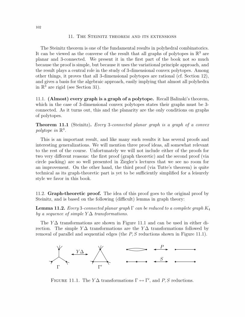
102

11. The Steinitz theorem and its extensions

The Steinitz theorem is one of the fundamental results in polyhedral combinatorics.It can be viewed as the converse of the result that all graphs of polytopes in R3 areplanar and 3-connected. We present it in the first part of the book not so muchbecause the proof is simple, but because it uses the variational principle approach, andthe result plays a central role in the study of 3-dimensional convex polytopes. Amongother things, it proves that all 3-dimensional polytopes are rational (cf. Section 12),and gives a basis for the algebraic approach, easily implying that almost all polyhedrain R3 are rigid (see Section 31).

11.1. (Almost) every graph is a graph of a polytope. Recall Balinski’s theorem,which in the case of 3-dimensional convex polytopes states their graphs must be 3-connected. As it turns out, this and the planarity are the only conditions on graphsof polytopes.

Theorem 11.1 (Steinitz). Every 3-connected planar graph is a graph of a convexpolytope in R3.

This is an important result, and like many such results it has several proofs andinteresting generalizations. We will mention three proof ideas, all somewhat relevantto the rest of the course. Unfortunately we will not include either of the proofs fortwo very different reasons: the first proof (graph theoretic) and the second proof (viacircle packing) are so well presented in Ziegler’s lectures that we see no room foran improvement. On the other hand, the third proof (via Tutte’s theorem) is quitetechnical as its graph-theoretic part is yet to be sufficiently simplified for a leisurelystyle we favor in this book.

11.2. Graph-theoretic proof. The idea of this proof goes to the original proof bySteinitz, and is based on the following (difficult) lemma in graph theory:

Lemma 11.2. Every 3-connected planar graph Γ can be reduced to a complete graphK4

by a sequence of simple Y∆ transformations.

The Y∆ transformations are shown in Figure 11.1 and can be used in either di-rection. The simple Y∆ transformations are the Y∆ transformations followed byremoval of parallel and sequential edges (the P, S reductions shown in Figure 11.1).

Γ Γ′

Y∆P

S

Figure 11.1. The Y∆ transformations Γ↔ Γ′, and P, S reductions.

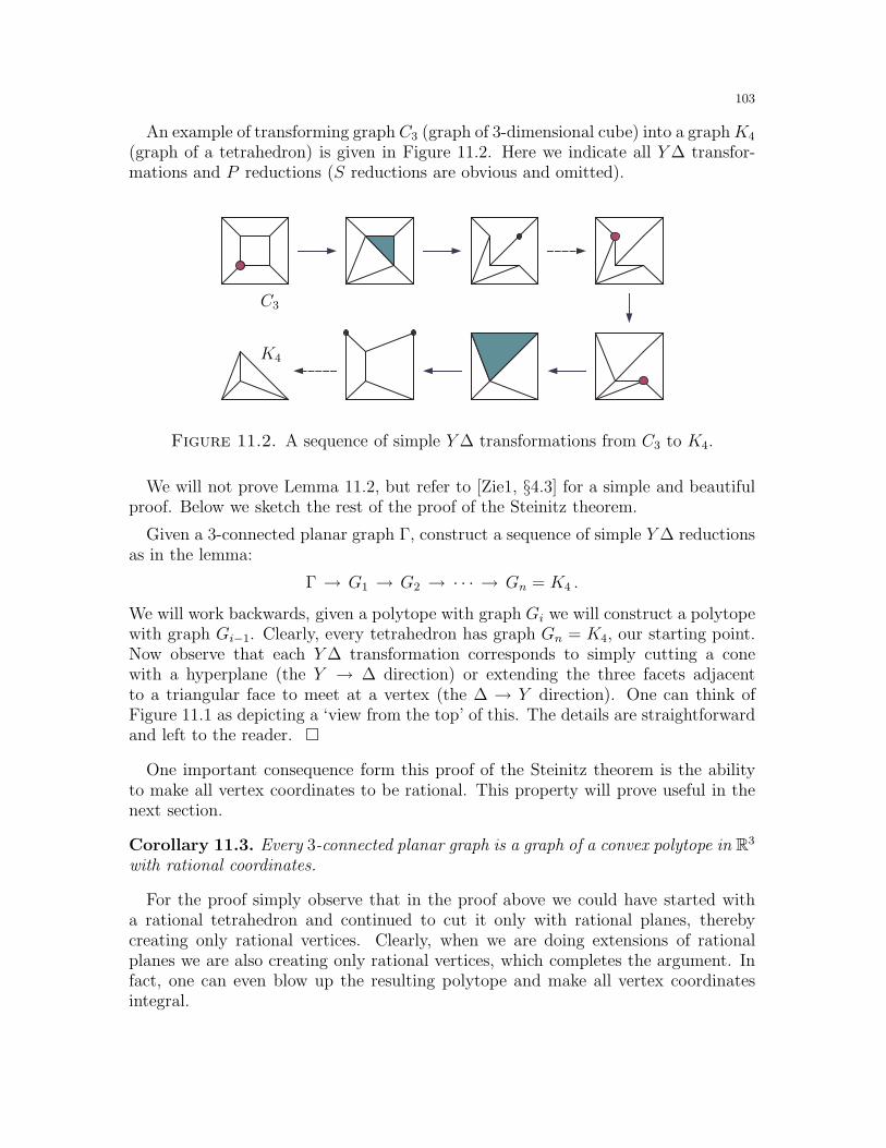
103

An example of transforming graph C3 (graph of 3-dimensional cube) into a graphK4

(graph of a tetrahedron) is given in Figure 11.2. Here we indicate all Y∆ transfor-mations and P reductions (S reductions are obvious and omitted).

C3

K4

Figure 11.2. A sequence of simple Y∆ transformations from C3 to K4.

We will not prove Lemma 11.2, but refer to [Zie1, §4.3] for a simple and beautifulproof. Below we sketch the rest of the proof of the Steinitz theorem.

Given a 3-connected planar graph Γ, construct a sequence of simple Y∆ reductionsas in the lemma:

Γ → G1 → G2 → · · · → Gn = K4 .

We will work backwards, given a polytope with graph Gi we will construct a polytopewith graph Gi−1. Clearly, every tetrahedron has graph Gn = K4, our starting point.Now observe that each Y∆ transformation corresponds to simply cutting a conewith a hyperplane (the Y → ∆ direction) or extending the three facets adjacentto a triangular face to meet at a vertex (the ∆ → Y direction). One can think ofFigure 11.1 as depicting a ‘view from the top’ of this. The details are straightforwardand left to the reader.

One important consequence form this proof of the Steinitz theorem is the abilityto make all vertex coordinates to be rational. This property will prove useful in thenext section.

Corollary 11.3. Every 3-connected planar graph is a graph of a convex polytope in R3

with rational coordinates.

For the proof simply observe that in the proof above we could have started witha rational tetrahedron and continued to cut it only with rational planes, therebycreating only rational vertices. Clearly, when we are doing extensions of rationalplanes we are also creating only rational vertices, which completes the argument. Infact, one can even blow up the resulting polytope and make all vertex coordinatesintegral.

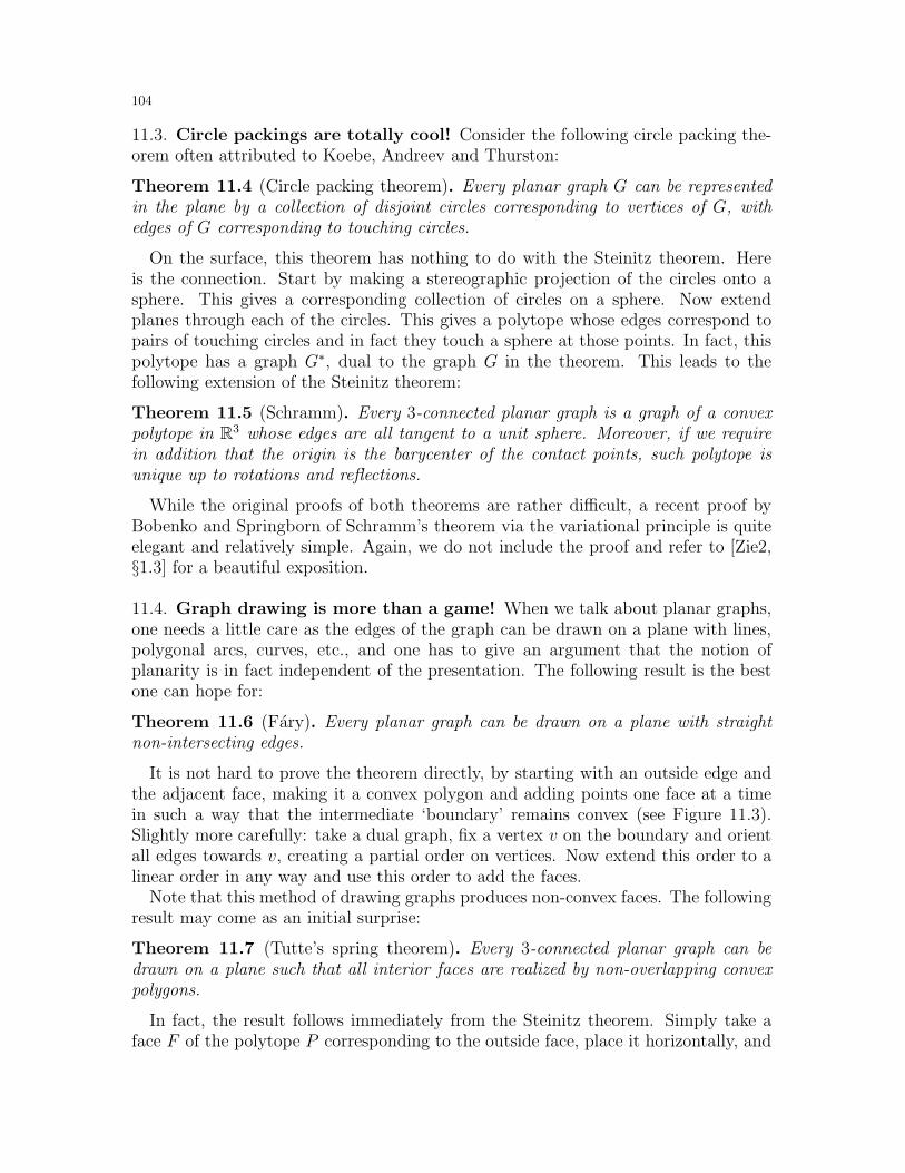
104

11.3. Circle packings are totally cool! Consider the following circle packing the-orem often attributed to Koebe, Andreev and Thurston:

Theorem 11.4 (Circle packing theorem). Every planar graph G can be representedin the plane by a collection of disjoint circles corresponding to vertices of G, withedges of G corresponding to touching circles.

On the surface, this theorem has nothing to do with the Steinitz theorem. Hereis the connection. Start by making a stereographic projection of the circles onto asphere. This gives a corresponding collection of circles on a sphere. Now extendplanes through each of the circles. This gives a polytope whose edges correspond topairs of touching circles and in fact they touch a sphere at those points. In fact, thispolytope has a graph G∗, dual to the graph G in the theorem. This leads to thefollowing extension of the Steinitz theorem:

Theorem 11.5 (Schramm). Every 3-connected planar graph is a graph of a convexpolytope in R3 whose edges are all tangent to a unit sphere. Moreover, if we requirein addition that the origin is the barycenter of the contact points, such polytope isunique up to rotations and reflections.

While the original proofs of both theorems are rather difficult, a recent proof byBobenko and Springborn of Schramm’s theorem via the variational principle is quiteelegant and relatively simple. Again, we do not include the proof and refer to [Zie2,§1.3] for a beautiful exposition.

11.4. Graph drawing is more than a game! When we talk about planar graphs,one needs a little care as the edges of the graph can be drawn on a plane with lines,polygonal arcs, curves, etc., and one has to give an argument that the notion ofplanarity is in fact independent of the presentation. The following result is the bestone can hope for:

Theorem 11.6 (Fary). Every planar graph can be drawn on a plane with straightnon-intersecting edges.

It is not hard to prove the theorem directly, by starting with an outside edge andthe adjacent face, making it a convex polygon and adding points one face at a timein such a way that the intermediate ‘boundary’ remains convex (see Figure 11.3).Slightly more carefully: take a dual graph, fix a vertex v on the boundary and orientall edges towards v, creating a partial order on vertices. Now extend this order to alinear order in any way and use this order to add the faces.

Note that this method of drawing graphs produces non-convex faces. The followingresult may come as an initial surprise:

Theorem 11.7 (Tutte’s spring theorem). Every 3-connected planar graph can bedrawn on a plane such that all interior faces are realized by non-overlapping convexpolygons.

In fact, the result follows immediately from the Steinitz theorem. Simply take aface F of the polytope P corresponding to the outside face, place it horizontally, and

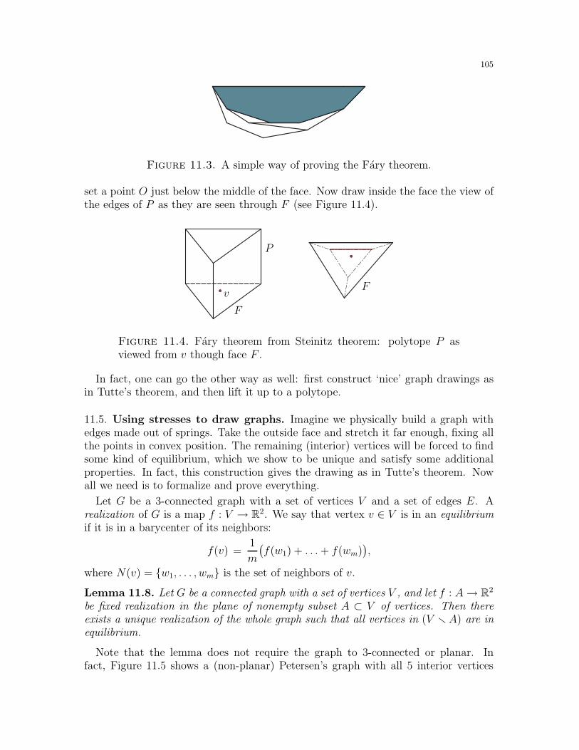
105

Figure 11.3. A simple way of proving the Fary theorem.

set a point O just below the middle of the face. Now draw inside the face the view ofthe edges of P as they are seen through F (see Figure 11.4).

P

F

F

v

Figure 11.4. Fary theorem from Steinitz theorem: polytope P asviewed from v though face F .

In fact, one can go the other way as well: first construct ‘nice’ graph drawings asin Tutte’s theorem, and then lift it up to a polytope.

11.5. Using stresses to draw graphs. Imagine we physically build a graph withedges made out of springs. Take the outside face and stretch it far enough, fixing allthe points in convex position. The remaining (interior) vertices will be forced to findsome kind of equilibrium, which we show to be unique and satisfy some additionalproperties. In fact, this construction gives the drawing as in Tutte’s theorem. Nowall we need is to formalize and prove everything.

Let G be a 3-connected graph with a set of vertices V and a set of edges E. Arealization of G is a map f : V → R2. We say that vertex v ∈ V is in an equilibriumif it is in a barycenter of its neighbors:

f(v) =1

m

(f(w1) + . . .+ f(wm)

),

where N(v) = w1, . . . , wm is the set of neighbors of v.

Lemma 11.8. Let G be a connected graph with a set of vertices V , and let f : A→ R2

be fixed realization in the plane of nonempty subset A ⊂ V of vertices. Then thereexists a unique realization of the whole graph such that all vertices in (V rA) are inequilibrium.

Note that the lemma does not require the graph to 3-connected or planar. Infact, Figure 11.5 shows a (non-planar) Petersen’s graph with all 5 interior vertices

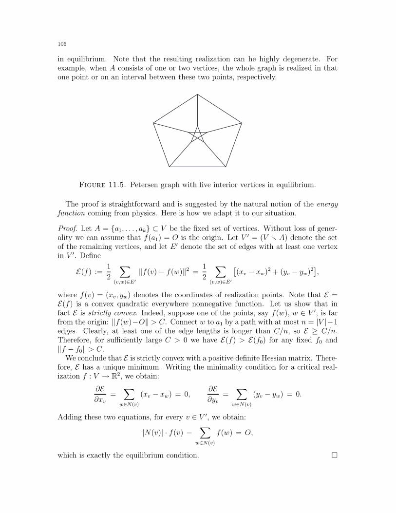
106

in equilibrium. Note that the resulting realization can he highly degenerate. Forexample, when A consists of one or two vertices, the whole graph is realized in thatone point or on an interval between these two points, respectively.

Figure 11.5. Petersen graph with five interior vertices in equilibrium.

The proof is straightforward and is suggested by the natural notion of the energyfunction coming from physics. Here is how we adapt it to our situation.

Proof. Let A = a1, . . . , ak ⊂ V be the fixed set of vertices. Without loss of gener-ality we can assume that f(a1) = O is the origin. Let V ′ = (V r A) denote the setof the remaining vertices, and let E ′ denote the set of edges with at least one vertexin V ′. Define

E(f) :=1

2

∑

(v,w)∈E′

‖f(v)− f(w)‖2 =1

2

∑

(v,w)∈E′

[(xv − xw)2 + (yv − yw)2

],

where f(v) = (xv, yw) denotes the coordinates of realization points. Note that E =E(f) is a convex quadratic everywhere nonnegative function. Let us show that infact E is strictly convex. Indeed, suppose one of the points, say f(w), w ∈ V ′, is farfrom the origin: ‖f(w)−O‖ > C. Connect w to a1 by a path with at most n = |V |−1edges. Clearly, at least one of the edge lengths is longer than C/n, so E ≥ C/n.Therefore, for sufficiently large C > 0 we have E(f) > E(f0) for any fixed f0 and‖f − f0‖ > C.

We conclude that E is strictly convex with a positive definite Hessian matrix. There-fore, E has a unique minimum. Writing the minimality condition for a critical real-ization f : V → R2, we obtain:

∂E∂xv

=∑

w∈N(v)

(xv − xw) = 0,∂E∂yv

=∑

w∈N(v)

(yv − yw) = 0.

Adding these two equations, for every v ∈ V ′, we obtain:

|N(v)| · f(v) −∑

w∈N(v)

f(w) = O,

which is exactly the equilibrium condition.

107

Note that the variational principle approach quickly reduced the problem to a graphtheoretic question. In fact, we do not even need the uniqueness part in the lemma— just the existence of the equilibrium configuration. Formally, the rest of the Tuttetheorem follows from the following (difficult) lemma.

Lemma 11.9. Let G = (V,E) be a 3-connected planar graph and let f : V → R2 beits realization. Suppose the outside face F forms a convex polygon and the remainingpoints in the realization are in equilibrium. Then all faces of G are disjoint convexpolygons.

The lemma is proved by a delicate and technical graph theoretic argument whichwe skip. Let us note, however, that Lemma 11.8 holds for all graphs, e.g., for acomplete graph Kn. On the other hand, the result of Lemma 11.9 obviously cannothold for non-planar graphs. Thus, planarity of G must be critical in the proof.

11.6. Exercises.

Exercise 11.1. Let P ⊂ R3 be a simple convex polytope whose faces are quadrilaterals.a) [1-] Prove that it has eight vertices.b) [1] Prove that P is combinatorially equivalent to a cube.c) [1] Prove that if seven vertices of P lie on a sphere, then so does the eighth vertex.

Exercise 11.2. [1] Let P ⊂ R3 be a simple convex polytope such that every face can beinscribed into a circle. Prove that P can be inscribed into a sphere.

Exercise 11.3. [1-] Let C ⊂ R3 be a convex cone with four faces. Prove that C has aninscribed sphere if and only if the opposite face angles have equal sums.

Exercise 11.4. a) [1+] Let P ⊂ R3 be a convex polytope whose faces are colored in blackand white such that no two black faces are adjacent. Suppose the total area of black facesis larger than the total area of white faces. Prove that P does not have an inscribed sphere.b) [1-] Find an example of such polytope P .c) [1-] Show that condition in part a) is necessary but not sufficient, even if there is aunique proper coloring of the faces.

Exercise 11.5. a) [1+] As above, let P ⊂ R3 be a convex polytope whose faces are coloredin black and white such that no two black faces are adjacent. Suppose the number of whitefaces is smaller than the number of black faces. Prove that P does not have an inscribedsphere.b) [1-] Let Q be a parallelepiped and let P be obtained from Q by cutting off the vertices.Use part a) to show that P does not have an inscribed sphere.

Exercise 11.6. a) [2] Let P be a convex polytope with graph Γ, and let C be a simplecycle in G. Prove that there exists a combinatorially equivalent polytope P ′, such that theedges of the boundary of a projection of P ′ correspond to C.b) [1] Prove that the shape of the polygon in the projection cannot be prescribed in advance.

Exercise 11.7. a) [1] Prove that for all k ≥ 3, a plane can be partitioned into k-gons(edge-to-edge).b) [2] For every simplicial convex polytope P ⊂ R3, prove that the space R3 can be parti-tioned into polytopes combinatorially equivalent to P (face-to-face).

108

c) [2] For every convex polytope P ⊂ R3, prove that the space R3 can be dissected intopolytopes combinatorially equivalent to P (not necessarily face-to-face).

Exercise 11.8. (Infinite Fary theorem) [2-] Let G be an infinite planar graph of boundeddegree. Prove that G can be drawn in the plane with straight edges. Check that thisgeneralizes part a) of the previous exercise.

11.7. Final remarks. Steinitz theorem was discovered by Ernst Steinitz in the late 1920sand his manuscript was published posthumously in 1934 by Hans Rademacher. For atraditional graph theoretic proof of the Steinitz theorem see e.g., [Gru4, §13.1], and for thehistory of the Steinitz theorem see [Gru5]. An attractive presentation of the graph theoreticproof is given in [Zie1, §4.3]. For the Bobenko–Springborn proof see [Zie2, §1] and [Spr](see also [Grub, §34]). An advanced generalization was obtained by Schramm, who showedthat the unit sphere plays no special role in Theorem 11.5, but in fact one can realize apolytope with edges tangent to any smooth convex body [Schra]. For a complete proof ofTutte’s spring theorem, the proof of the Steinitz theorem, references and details see [Ric](see also [Tho2]).

The reason Theorem 11.4 is attributed to the three authors is because Koebe claimed itin 1936, but proved it only for triangulations. Almost half a century later, in 1985, Thurstongave a talk where he presented the theorem. He also noted in his book (which remainedunpublished for years) that the result follows easily from Andreev’s results of the 1970.Only then, with papers by Colin de Verdiere (1988), Schramm (1991), and others, theresult was brought into prominence. We refer to [Ber2] for an elementary introduction,to [PacA, Ch. 8] for a nicely written standard fixed-point type proof, and to [Spr, Zie2] forthe references.

It is interesting to note a fundamental difference between the two variational proofs (ofTheorems 11.5 and 11.7). While in the proof of Tutte’s theorem proving existence of anequilibrium is easy, it is showing that the equilibrium is what we want that is hard. Theopposite is true in the Bobenko-Springborn proof (as well as in Schramm’s proof) it isproving the existence of an equilibrium that is hard; showing that the equilibrium producesa desired configuration is quite easy.

109

12. Universality of point and line configurations

This is the first of two sections on universality. In essence, it shows that theface combinatorics studied in Section 8 and the geometry of polyhedra are largelyincompatible. To put it another way, we show that by making some restrictions onthe face lattice one can ensure that the polytopes are irrational, as complicated asneeded, or even non-existent. This is an extremely negative result showing that thereis no hope for the Steinitz type theorem in higher dimensions (see Section 11).

12.1. Universality is not for everyone. In the following two sections we presentseveral results with one unifying goal: to show that various constructions and con-figurations in discrete geometry can encode an extremely wide (universal!) rangeof objects. While this may seem an empowering proposition, from the postmodernpoint of view this is very disappointing, since we are basically saying that nothinginteresting can be proved about all these general geometric objects. Indeed, what canpossibly be interesting about everything?

12.2. Ruler and compass constructions are so passe. Recall that it is impossibleto construct a regular 7-gon using a compass and a ruler. This classical result ofGauss is now considered iconic, but two hundred years ago the result took awhile tounderstand and appreciate. What was more impressive to mathematicians of the daywas the construction of a regular 17-gon, unknown until Gauss. This constructivepart of his work is considered elementary now, but his approach, in fact, can beviewed as the earliest universality type result.

Consider an increasing sequence of fields

K0 ⊂ K1 ⊂ K2 ⊂ . . . ⊂ Kn ,

where K0 = Q, Ki = Ki−1[√ai], and ai ∈ Ki−1, for all 1 ≤ i ≤ n. We call a number

z ∈ C geometric if there exist a chain of fields as above, such that z ∈ Kn, forsome n ∈ N.

Theorem 12.1 (Gauss). Every geometric number can be constructed by the ruler andthe compass.

We need to elaborate on what we mean by the ruler and compass construction (inthe plane). We identify the plane with the field C, and assume that in the beginningare given the set of two points A0 = 0, 1. Our algorithm increases the set of pointsby making the ruler and compass drawing, and adding new intersection points at eachstep.

Formally, suppose at the n-th step we have the set An ⊂ C of points in the plane.At the (n+ 1)-th step we can do two of the following operations:

• draw a line (ai, aj) through any two points ai, aj ∈ An, or• draw a circle with a center at ak and radius |aiaj|, for some ai, aj, ak ∈ An.

Then we can add the set of intersection point(s) B = b1, b2 in the case of two circles,or a line and a circle, and B = b in case two lines, to the set of points:

• let An+1 := An ∪ B.

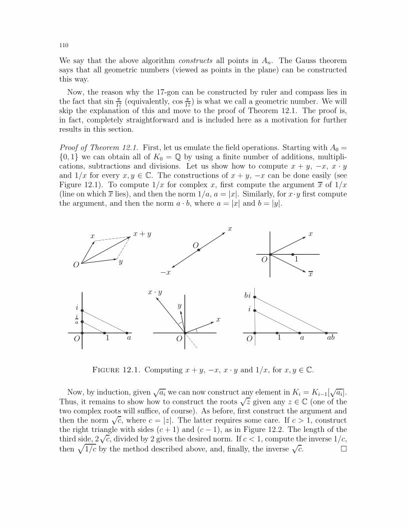
110

We say that the above algorithm constructs all points in An. The Gauss theoremsays that all geometric numbers (viewed as points in the plane) can be constructedthis way.

Now, the reason why the 17-gon can be constructed by ruler and compass lies inthe fact that sin π

17(equivalently, cos π

17) is what we call a geometric number. We will

skip the explanation of this and move to the proof of Theorem 12.1. The proof is,in fact, completely straightforward and is included here as a motivation for furtherresults in this section.

Proof of Theorem 12.1. First, let us emulate the field operations. Starting with A0 =0, 1 we can obtain all of K0 = Q by using a finite number of additions, multipli-cations, subtractions and divisions. Let us show how to compute x + y, −x, x · yand 1/x for every x, y ∈ C. The constructions of x + y, −x can be done easily (seeFigure 12.1). To compute 1/x for complex x, first compute the argument x of 1/x(line on which x lies), and then the norm 1/a, a = |x|. Similarly, for x·y first computethe argument, and then the norm a · b, where a = |x| and b = |y|.

O OO

O

O

O

x

xx

x

−x

y

y

x+ y

x

x · y

a 11

1

ia

ii

bi

a ab

Figure 12.1. Computing x+ y, −x, x · y and 1/x, for x, y ∈ C.

Now, by induction, given√ai we can now construct any element in Ki = Ki−1[

√ai].

Thus, it remains to show how to construct the roots√z given any z ∈ C (one of the

two complex roots will suffice, of course). As before, first construct the argument andthen the norm

√c, where c = |z|. The latter requires some care. If c > 1, construct

the right triangle with sides (c+ 1) and (c− 1), as in Figure 12.2. The length of thethird side, 2

√c, divided by 2 gives the desired norm. If c < 1, compute the inverse 1/c,

then√

1/c by the method described above, and, finally, the inverse√c.

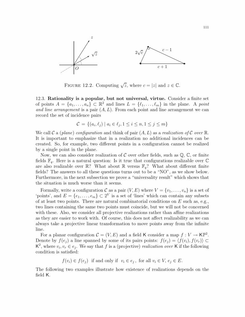
111

O

z

√z 2

√c

c+ 1

c− 1

Figure 12.2. Computing√z, where c = |z| and z ∈ C.

12.3. Rationality is a popular, but not universal, virtue. Consider a finite setof points A = a1, . . . , an ⊂ R2 and lines L = ℓ1, . . . , ℓm in the plane. A pointand line arrangement is a pair (A,L). From each point and line arrangement we canrecord the set of incidence pairs

C = (ai, ℓj) | ai ∈ ℓj, 1 ≤ i ≤ n, 1 ≤ j ≤ mWe call C a (plane) configuration and think of pair (A,L) as a realization of C over R.It is important to emphasize that in a realization no additional incidences can becreated. So, for example, two different points in a configuration cannot be realizedby a single point in the plane.

Now, we can also consider realization of C over other fields, such as Q, C, or finitefields Fq. Here is a natural question: Is it true that configurations realizable over Care also realizable over R? What about R versus Fq? What about different finitefields? The answers to all these questions turns out to be a “NO”, as we show below.Furthermore, in the next subsection we prove a “universality result” which shows thatthe situation is much worse than it seems.

Formally, write a configuration C as a pair (V,E) where V = v1, . . . , vn is a set of‘points’, and E = e1, . . . , em ⊂ 2V is a set of ‘lines’ which can contain any subsetsof at least two points. There are natural combinatorial conditions on E such as, e.g.,two lines containing the same two points must coincide, but we will not be concernedwith these. Also, we consider all projective realizations rather than affine realizationsas they are easier to work with. Of course, this does not affect realizability as we canalways take a projective linear transformation to move points away from the infiniteline.

For a planar configuration C = (V,E) and a field K consider a map f : V → KP2.Denote by f(ej) a line spanned by some of its pairs points: f(ej) = 〈f(vi), f(vr)〉 ⊂K

2, where vi, vr ∈ ej . We say that f is a (projective) realization over K if the followingcondition is satisfied:

f(vi) ∈ f(ej) if and only if vi ∈ ej , for all vi ∈ V, ej ∈ E.The following two examples illustrate how existence of realizations depends on thefield K.

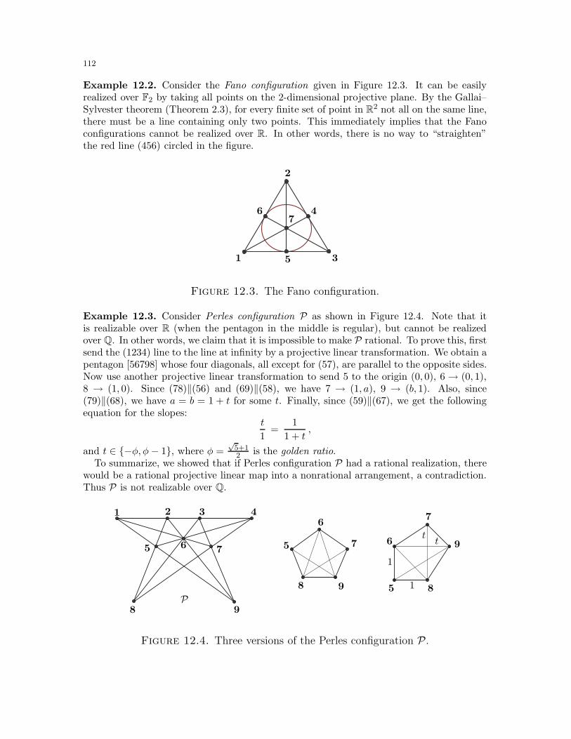
112

Example 12.2. Consider the Fano configuration given in Figure 12.3. It can be easilyrealized over F2 by taking all points on the 2-dimensional projective plane. By the Gallai–Sylvester theorem (Theorem 2.3), for every finite set of point in R2 not all on the same line,there must be a line containing only two points. This immediately implies that the Fanoconfigurations cannot be realized over R. In other words, there is no way to “straighten”the red line (456) circled in the figure.

1

2

3

4

5

67

Figure 12.3. The Fano configuration.

Example 12.3. Consider Perles configuration P as shown in Figure 12.4. Note that itis realizable over R (when the pentagon in the middle is regular), but cannot be realizedover Q. In other words, we claim that it is impossible to make P rational. To prove this, firstsend the (1234) line to the line at infinity by a projective linear transformation. We obtain apentagon [56798] whose four diagonals, all except for (57), are parallel to the opposite sides.Now use another projective linear transformation to send 5 to the origin (0, 0), 6→ (0, 1),8 → (1, 0). Since (78)‖(56) and (69)‖(58), we have 7 → (1, a), 9 → (b, 1). Also, since(79)‖(68), we have a = b = 1 + t for some t. Finally, since (59)‖(67), we get the followingequation for the slopes:

t

1=

1

1 + t,

and t ∈ −φ, φ− 1, where φ =√

5+12 is the golden ratio.

To summarize, we showed that if Perles configuration P had a rational realization, therewould be a rational projective linear map into a nonrational arrangement, a contradiction.Thus P is not realizable over Q.

1 2 3 4

5

556

6

6

7

77

88

8

9

9

9

1

1

tt

P

Figure 12.4. Three versions of the Perles configuration P.

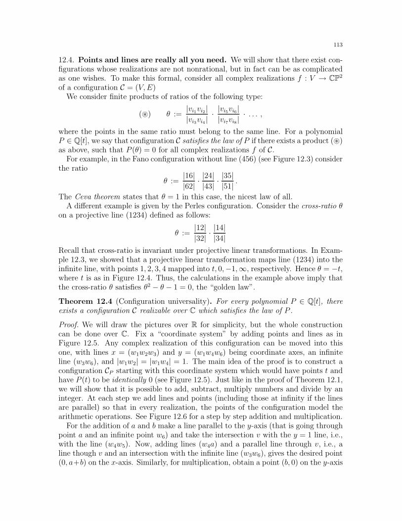
113

12.4. Points and lines are really all you need. We will show that there exist con-figurations whose realizations are not nonrational, but in fact can be as complicatedas one wishes. To make this formal, consider all complex realizations f : V → CP2

of a configuration C = (V,E)We consider finite products of ratios of the following type:

(⊛) θ :=|vi1vi2 ||vi3vi4 |

· |vi5vi6 ||vi7vi8 |· . . . ,

where the points in the same ratio must belong to the same line. For a polynomialP ∈ Q[t], we say that configuration C satisfies the law of P if there exists a product (⊛)as above, such that P (θ) = 0 for all complex realizations f of C.

For example, in the Fano configuration without line (456) (see Figure 12.3) considerthe ratio

θ :=|16||62| ·

|24||43| ·

|35||51| .

The Ceva theorem states that θ = 1 in this case, the nicest law of all.A different example is given by the Perles configuration. Consider the cross-ratio θ

on a projective line (1234) defined as follows:

θ :=|12||32| ·

|14||34|

Recall that cross-ratio is invariant under projective linear transformations. In Exam-ple 12.3, we showed that a projective linear transformation maps line (1234) into theinfinite line, with points 1, 2, 3, 4 mapped into t, 0,−1,∞, respectively. Hence θ = −t,where t is as in Figure 12.4. Thus, the calculations in the example above imply thatthe cross-ratio θ satisfies θ2 − θ − 1 = 0, the “golden law”.

Theorem 12.4 (Configuration universality). For every polynomial P ∈ Q[t], thereexists a configuration C realizable over C which satisfies the law of P .

Proof. We will draw the pictures over R for simplicity, but the whole constructioncan be done over C. Fix a “coordinate system” by adding points and lines as inFigure 12.5. Any complex realization of this configuration can be moved into thisone, with lines x = (w1w2w3) and y = (w1w4w6) being coordinate axes, an infiniteline (w3w6), and |w1w2| = |w1w4| = 1. The main idea of the proof is to construct aconfiguration CP starting with this coordinate system which would have points t andhave P (t) to be identically 0 (see Figure 12.5). Just like in the proof of Theorem 12.1,we will show that it is possible to add, subtract, multiply numbers and divide by aninteger. At each step we add lines and points (including those at infinity if the linesare parallel) so that in every realization, the points of the configuration model thearithmetic operations. See Figure 12.6 for a step by step addition and multiplication.

For the addition of a and b make a line parallel to the y-axis (that is going throughpoint a and an infinite point w6) and take the intersection v with the y = 1 line, i.e.,with the line (w4w5). Now, adding lines (w4a) and a parallel line through v, i.e., aline though v and an intersection with the infinite line (w3w6), gives the desired point(0, a+b) on the x-axis. Similarly, for multiplication, obtain a point (b, 0) on the y-axis

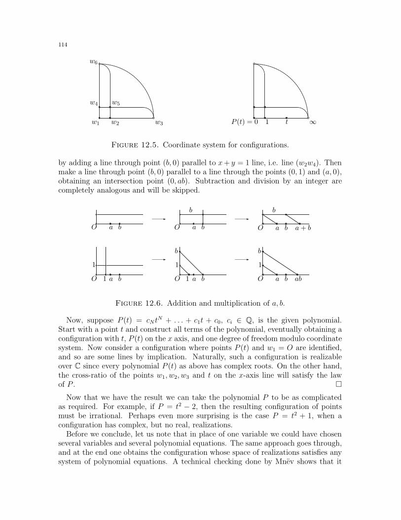
114

w1 w2 w3

w4 w5

w6

P (t) = 0 1 ∞t

Figure 12.5. Coordinate system for configurations.

by adding a line through point (b, 0) parallel to x+ y = 1 line, i.e. line (w2w4). Thenmake a line through point (b, 0) parallel to a line through the points (0, 1) and (a, 0),obtaining an intersection point (0, ab). Subtraction and division by an integer arecompletely analogous and will be skipped.

1

1

1

1

1

aa

aa

a

a

b

b

b

b

bb

b

b

ab

a+ b

OO

OO

O

O

bb

Figure 12.6. Addition and multiplication of a, b.

Now, suppose P (t) = cN tN + . . . + c1t + c0, ci ∈ Q, is the given polynomial.

Start with a point t and construct all terms of the polynomial, eventually obtaining aconfiguration with t, P (t) on the x axis, and one degree of freedom modulo coordinatesystem. Now consider a configuration where points P (t) and w1 = O are identified,and so are some lines by implication. Naturally, such a configuration is realizableover C since every polynomial P (t) as above has complex roots. On the other hand,the cross-ratio of the points w1, w2, w3 and t on the x-axis line will satisfy the lawof P .

Now that we have the result we can take the polynomial P to be as complicatedas required. For example, if P = t2 − 2, then the resulting configuration of pointsmust be irrational. Perhaps even more surprising is the case P = t2 + 1, when aconfiguration has complex, but no real, realizations.

Before we conclude, let us note that in place of one variable we could have chosenseveral variables and several polynomial equations. The same approach goes through,and at the end one obtains the configuration whose space of realizations satisfies anysystem of polynomial equations. A technical checking done by Mnev shows that it

115

is always possible to proceed with this without ever creating any extra equations.We leave all this aside. The main point of this subsection is to emphasize that in acertain sense (which can be made completely formal), all algebraic varieties over Qare encoded by finite configurations.

12.5. Polytopes can also be irrational! Let P ⊂ Rd be a convex polytope, andlet L be the poset (lattice) of faces of P . We say that P ′ ⊂ Rd is combinatoriallyequivalent to P if they have the same poset L. We say that P is realizable over asubfield K ⊂ R if there is a polytope P ′ combinatorially equivalent to P , such thatall coordinates of P ′ lie in K. As it turns out, just like in case of realizations of pointsand lines, there exist polytopes which satisfy any prescribed law.

Theorem 12.5 (Perles, Mnev). There exists a polytope P ⊂ Rd which cannot berealized over Q. Moreover, there exists a polytope P ⊂ Rd which cannot be realizedover any finite extension of Q.

Perles configuration (see Example 12.3) appeared in his original construction ofan irrational polytope. This result may seem harder and unintuitive since in threedimensions this cannot happen: Corollary 11.3 of the Steinitz theorem asserts thatall convex 3-dimensional polytopes are rational. Let us show first how to constructa polytope from a point and line configuration, and establish a direct map betweentheir realization spaces.

The Lawrence construction. Think of a plane configuration C as a collection of vectorsV = v1, . . . , vn ⊂ R3, obtained by mapping points (x, y) into (x, y, 1). Clearly, threepoints lie on a line if they are mapped into linearly dependent vectors. Now considera vector space R3 × Rn with the configuration C in R3, and an auxiliary space Rn

spanned by vectors w1, . . . , wn. Now consider a polytope PC given by a convex hullof points

xi = (vi, wi), yi = (vi, 2wi), where xi, yi ∈ R3 × Rn, 1 ≤ i ≤ n.

The polytope PC has a special combinatorial structure so that the linear relations (onvertices) inherit all linear relations of C. To see this, notice that points xi, yi | i ∈ Iare always in convex position, and thus they lie on a facet if and only if

∑

i∈I(2xi − yi) =

∑

i∈I(vi, O) = (O,O),

i.e., when the points vi | i ∈ I ⊂ V lie on the same line in C.From the construction, we immediately conclude that if C is irrational (cannot be

realized over Q), as in Example 12.3, then so is the polytope PC. More generally, ifa field K is a finite extension of Q, then there exists a polynomial P with rationalcoefficients and roots not in K. By the configuration universality theorem there existsa configuration C which satisfies the law of P . Then the corresponding polytope PCcannot be realized over K.

116

12.6. Exercises.

Exercise 12.1. [1] Prove that the center of a circle can be constructed by using only acompass (i.e., without a ruler).

Exercise 12.2. a) [1+] Prove that using the ruler, compass and angle-trisector one canconstruct a regular heptagon.b) [2] Prove that a real cubic equation can be solved geometrically using a ruler, compassand angle-trisector if and only if its roots are all real.

Exercise 12.3. a) [1] Suppose a1, . . . , an > 0. Find the necessary and sufficient conditionsfor the existence of an n-gon with these edge lengths to be inscribed into a circle.b) [2-] Prove that for n ≥ 5, the radius of this circle cannot be constructed with a rulerand a compass (given edge lengths ai).

Exercise 12.4. [1+] A geometry problem asks to use a ruler and compass to find a squarewith two vertices on each of the two given non-intersecting circles. Show how to solve it orprove that this is impossible in general.

Exercise 12.5. [1] The y = x2 parabola is given, but the axes are erased. Reconstruct theaxes using ruler and compass.

Exercise 12.6. [1] Prove that a regular pentagon cannot be realized in Q3. Conclude thatthe regular icosahedron cannot be realized in Q3.

Exercise 12.7. [1] The Pappus theorem states that for every two triples of points on twolines: a, b, c ∈ L and a′, b′, c′ ∈ L′ the points of intersection of x = (a, b′)∩(a′, b), y = (a, c′)∩(a′, c), z = (b, c′)∩ (b′, c) must lie on a line. Remove this extra line to obtain a configurationwith nine points and eight lines. Convert the Pappus theorem into a realizability result ofthis configuration over R. Can this configuration be realized over C or over a finite field?

Exercise 12.8. [2] Find a (self-intersecting) polyhedral surface in R3 which cannot berealized over Q.

Exercise 12.9. [2-] Find the analogue of Theorem 12.4 for polytopes. In other words,prove a universality type theorem which extends Theorem 12.5.

12.7. Final remarks. Thinking of Theorem 12.1 as a universality result is a classical idea(see [CouR, Ch. III §2]). Our writing was influenced by a terrific essay [Man]. Let usmention a well-known result by Mohr and Mascheroni, which asserts that every constructionwith a ruler and a compass is possible using a compass alone (see [CouR, Ch. III §5]).In a different direction, Steiner showed that given a fixed circle and its center, all theconstructions in the plane can be carried out by the ruler alone. We refer to classicaltextbooks [Bieb, Leb2] for these and other results on geometric constructions (see also [Adl,Schr1]), and to [Hun, Kos, Mar, Smo] for an introduction (see also nice exercises in [CouR,Ch. IV §7]). Finally, an interesting complexity result comparing capabilities of two tools isgiven in [ABe].

Realizability of point and line configurations over fields is a part of the much more generalsubject of matroid theory. In a different direction, connections between various geometriesgo beyond realizability over fields, as there exist geometries without Desargues’ theorem,etc. [Hil, Kag2].

117

What we call “Perles configuration” is the point and line configuration which appears in

Perles’s construction of the first non-rational polytope [Gru4, §3.5]. Theorem 12.4 is a weak

version of the Mnev Universality Theorem. For the introduction to the Mnev theorem and

the Lawrence construction see [Zie1, §6.6] and the original paper [Mnev]. The full proof of

the Mnev theorem, further extensions and references can be found in [Ric].

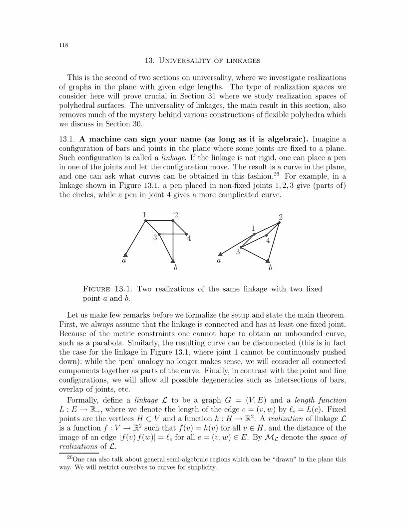
118

13. Universality of linkages

This is the second of two sections on universality, where we investigate realizationsof graphs in the plane with given edge lengths. The type of realization spaces weconsider here will prove crucial in Section 31 where we study realization spaces ofpolyhedral surfaces. The universality of linkages, the main result in this section, alsoremoves much of the mystery behind various constructions of flexible polyhedra whichwe discuss in Section 30.

13.1. A machine can sign your name (as long as it is algebraic). Imagine aconfiguration of bars and joints in the plane where some joints are fixed to a plane.Such configuration is called a linkage. If the linkage is not rigid, one can place a penin one of the joints and let the configuration move. The result is a curve in the plane,and one can ask what curves can be obtained in this fashion.26 For example, in alinkage shown in Figure 13.1, a pen placed in non-fixed joints 1, 2, 3 give (parts of)the circles, while a pen in joint 4 gives a more complicated curve.

1

1 22

3

3 44

bbaa

Figure 13.1. Two realizations of the same linkage with two fixedpoint a and b.

Let us make few remarks before we formalize the setup and state the main theorem.First, we always assume that the linkage is connected and has at least one fixed joint.Because of the metric constraints one cannot hope to obtain an unbounded curve,such as a parabola. Similarly, the resulting curve can be disconnected (this is in factthe case for the linkage in Figure 13.1, where joint 1 cannot be continuously pusheddown); while the ‘pen’ analogy no longer makes sense, we will consider all connectedcomponents together as parts of the curve. Finally, in contrast with the point and lineconfigurations, we will allow all possible degeneracies such as intersections of bars,overlap of joints, etc.

Formally, define a linkage L to be a graph G = (V,E) and a length functionL : E → R+, where we denote the length of the edge e = (v, w) by ℓe = L(e). Fixedpoints are the vertices H ⊂ V and a function h : H → R2. A realization of linkage Lis a function f : V → R2 such that f(v) = h(v) for all v ∈ H , and the distance of theimage of an edge |f(v)f(w)| = ℓe for all e = (v, w) ∈ E. ByML denote the space ofrealizations of L.

26One can also talk about general semi-algebraic regions which can be “drawn” in the plane thisway. We will restrict ourselves to curves for simplicity.

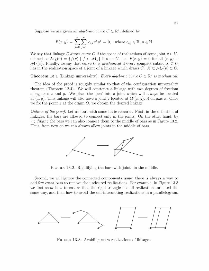
119

Suppose we are given an algebraic curve C ⊂ R2, defined by

F (x, y) =

n∑

i=0

n∑

j=0

ci,j xi yj = 0, where ci,j ∈ R, n ∈ N.

We say that linkage L draws curve C if the space of realizations of some joint v ∈ V ,defined as ML(v) = f(v) | f ∈ ML lies on C, i.e. F (x, y) = 0 for all (x, y) ∈ML(v). Finally, we say that curve C is mechanical if every compact subset X ⊂ Clies in the realization space of a joint of a linkage which draws C: X ⊂ML(v) ⊂ C.

Theorem 13.1 (Linkage universality). Every algebraic curve C ⊂ R2 is mechanical.

The idea of the proof is roughly similar to that of the configuration universalitytheorem (Theorem 12.4). We will construct a linkage with two degrees of freedomalong axes x and y. We place the ‘pen’ into a joint which will always be locatedat (x, y). This linkage will also have a joint z located at (F (x, y), 0) on axis x. Oncewe fix the point z at the origin O, we obtain the desired linkage.

Outline of the proof. Let us start with some basic remarks. First, in the definition oflinkages, the bars are allowed to connect only in the joints. On the other hand, byrigidifying the bars we can also connect them to the middle of bars as in Figure 13.2.Thus, from now on we can always allow joints in the middle of bars.

Figure 13.2. Rigidifying the bars with joints in the middle.

Second, we will ignore the connected components issue: there is always a way toadd few extra bars to remove the undesired realizations. For example, in Figure 13.3we first show how to ensure that the rigid triangle has all realizations oriented thesame way, and then how to avoid the self-intersecting realizations in a parallelogram.

Figure 13.3. Avoiding extra realizations of linkages.

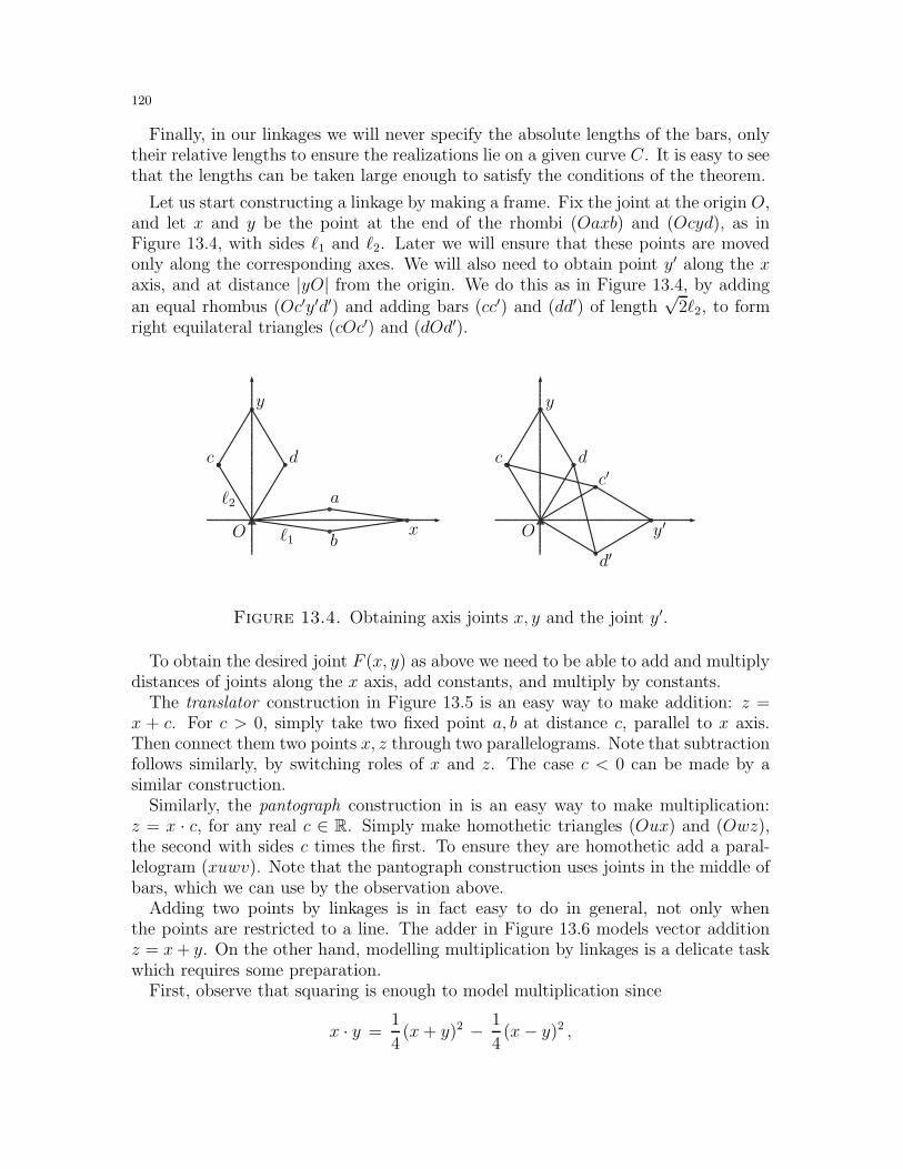
120

Finally, in our linkages we will never specify the absolute lengths of the bars, onlytheir relative lengths to ensure the realizations lie on a given curve C. It is easy to seethat the lengths can be taken large enough to satisfy the conditions of the theorem.

Let us start constructing a linkage by making a frame. Fix the joint at the origin O,and let x and y be the point at the end of the rhombi (Oaxb) and (Ocyd), as inFigure 13.4, with sides ℓ1 and ℓ2. Later we will ensure that these points are movedonly along the corresponding axes. We will also need to obtain point y′ along the xaxis, and at distance |yO| from the origin. We do this as in Figure 13.4, by addingan equal rhombus (Oc′y′d′) and adding bars (cc′) and (dd′) of length

√2ℓ2, to form

right equilateral triangles (cOc′) and (dOd′).

ℓ1

ℓ2

OO

c cd dc′

d′

a

bx

yy

y′

Figure 13.4. Obtaining axis joints x, y and the joint y′.

To obtain the desired joint F (x, y) as above we need to be able to add and multiplydistances of joints along the x axis, add constants, and multiply by constants.

The translator construction in Figure 13.5 is an easy way to make addition: z =x + c. For c > 0, simply take two fixed point a, b at distance c, parallel to x axis.Then connect them two points x, z through two parallelograms. Note that subtractionfollows similarly, by switching roles of x and z. The case c < 0 can be made by asimilar construction.

Similarly, the pantograph construction in is an easy way to make multiplication:z = x · c, for any real c ∈ R. Simply make homothetic triangles (Oux) and (Owz),the second with sides c times the first. To ensure they are homothetic add a paral-lelogram (xuwv). Note that the pantograph construction uses joints in the middle ofbars, which we can use by the observation above.

Adding two points by linkages is in fact easy to do in general, not only whenthe points are restricted to a line. The adder in Figure 13.6 models vector additionz = x+ y. On the other hand, modelling multiplication by linkages is a delicate taskwhich requires some preparation.

First, observe that squaring is enough to model multiplication since

x · y =1

4(x+ y)2 − 1

4(x− y)2 ,

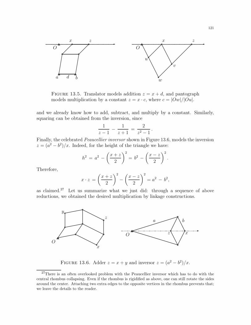
121

OO

a bd

xx

u

v

w

zz

Figure 13.5. Translator models addition z = x+ d, and pantographmodels multiplication by a constant z = x · c, where c = |Ow|/|Ou|.

and we already know how to add, subtract, and multiply by a constant. Similarly,squaring can be obtained from the inversion, since

1

z − 1− 1

z + 1=

2

z2 − 1.

Finally, the celebrated Peaucellier inversor shown in Figure 13.6, models the inversionz = (a2 − b2)/x. Indeed, for the height of the triangle we have:

h2 = a2 −(x+ z

2

)2

= b2 −(x− z

2

)2

.

Therefore,

x · z =

(x+ z

2

)2

−(x− z

2

)2

= a2 − b2,

as claimed.27 Let us summarize what we just did: through a sequence of abovereductions, we obtained the desired multiplication by linkage constructions.

O

O

a b

y

x

x

z

z

Figure 13.6. Adder z = x+ y and inversor z = (a2 − b2)/x.

27There is an often overlooked problem with the Peaucellier inversor which has to do with thecentral rhombus collapsing. Even if the rhombus is rigidified as above, one can still rotate the sidesaround the center. Attaching two extra edges to the opposite vertices in the rhombus prevents that;we leave the details to the reader.

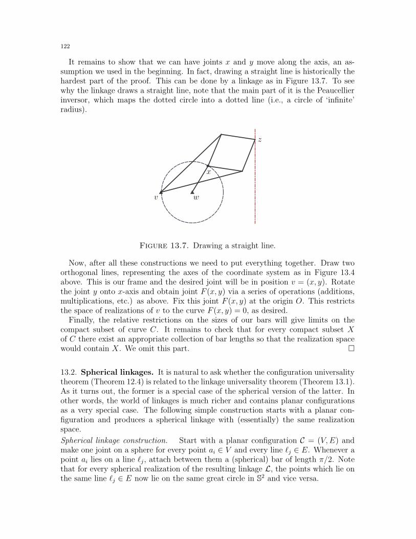
122

It remains to show that we can have joints x and y move along the axis, an as-sumption we used in the beginning. In fact, drawing a straight line is historically thehardest part of the proof. This can be done by a linkage as in Figure 13.7. To seewhy the linkage draws a straight line, note that the main part of it is the Peaucellierinversor, which maps the dotted circle into a dotted line (i.e., a circle of ‘infinite’radius).

v w

x

z

Figure 13.7. Drawing a straight line.

Now, after all these constructions we need to put everything together. Draw twoorthogonal lines, representing the axes of the coordinate system as in Figure 13.4above. This is our frame and the desired joint will be in position v = (x, y). Rotatethe joint y onto x-axis and obtain joint F (x, y) via a series of operations (additions,multiplications, etc.) as above. Fix this joint F (x, y) at the origin O. This restrictsthe space of realizations of v to the curve F (x, y) = 0, as desired.

Finally, the relative restrictions on the sizes of our bars will give limits on thecompact subset of curve C. It remains to check that for every compact subset Xof C there exist an appropriate collection of bar lengths so that the realization spacewould contain X. We omit this part.

13.2. Spherical linkages. It is natural to ask whether the configuration universalitytheorem (Theorem 12.4) is related to the linkage universality theorem (Theorem 13.1).As it turns out, the former is a special case of the spherical version of the latter. Inother words, the world of linkages is much richer and contains planar configurationsas a very special case. The following simple construction starts with a planar con-figuration and produces a spherical linkage with (essentially) the same realizationspace.

Spherical linkage construction. Start with a planar configuration C = (V,E) andmake one joint on a sphere for every point ai ∈ V and every line ℓj ∈ E. Whenever apoint ai lies on a line ℓj , attach between them a (spherical) bar of length π/2. Notethat for every spherical realization of the resulting linkage L, the points which lie onthe same line ℓj ∈ E now lie on the same great circle in S2 and vice versa.

123

In order to make this construction completely rigorous and straightforward oneneeds to substitute S2 with RP2 and consider all projective realizations of C. Weleave the details to the reader.

13.3. Exercises.

Exercise 13.1. [1+] Give an explicit construction of a linkage which draws a regular pen-tagon.

Exercise 13.2. [1+] Give an explicit construction of a linkage which draws an ellipse withdistinct axes.

Exercise 13.3. [2-] Prove that 3-dimensional algebraic curves and surfaces can be drawnby 3-dimensional linkages.

Exercise 13.4. Define a spherical polygon [x1 . . . xn] ⊂ S2 to be the union of geodesicarcs [xixi+1] on a unit sphere. Denote by L the set of sequences of lengths of these arcs:

(ℓ1, . . . , ℓn), where ℓi = |xixi+1|S2 .

a) [1-] Prove that if a sequence (ℓ1, . . . , ℓn) ∈ L then so does every permutation (ℓσ(1), . . . , ℓσ(n)),σ ∈ Sn.b) [2-] Prove that (ℓ1, . . . , ℓn) ∈ L if and only if

0 ≤ ℓi ≤ π, for all 1 ≤ i ≤ n, and∑

i∈Iℓi ≤

∑

j /∈Iℓj +

(|I| − 1

)π, for all I ⊂ [n], |I| odd.

c) [1] Prove that the inequalities in part b) are non-redundant.

13.4. Final remarks. The study of linkages is long, classical and exciting. It becamepopular with Watt’s discovery in 1784 of a linkage which approximately translates a forwardinto a circular motion. This mechanical linkage has been used in trains and is still in usein many car models. Chebyshev studied Watt’s linkage for thirty years and introduced hisown linkages. Interestingly, he believed that a linkage which draws a line is impossible toconstruct and introduced the Chebyshev polynomials in an effort to approximate the linewith low degree polynomials. Somewhat unusually, Peaucellier announced his discovery ina letter in 1871 without a hint to the actual construction, so in 1873 it was independentlyrediscovered by Lipkin. We refer to [CouR, Ch. III §5.4] and [HilC, §40] for the introductorytreatment, and to a celebrated lecture by Kempe [Kem] who essentially proved our linkageuniversality theorem (Theorem 13.1). For the story of interesting polyhedral linkages inthree dimensions see [Gol1].

The universality of linkages idea was first proposed by Kempe and Lebesgue (see above),and was revived by Thurston who popularized it with a saying “there exists a linkage whichsigns your name”[King]. These results were recently extended and formalized in a powerfulpaper by Kapovich and Millson [KM4] (see also [King]). Our Theorem 13.1 is a toy versionof their results, which are much more technical and precise. On the other hand, the basicidea can already be seen in the proof above. Finally, the connection between sphericallinkages and planar configurations was found in [KM2].

Let us mention that throughout history kinematics has been an honorable field of study,

and some of the linkages described above (such as the pantograph) have been used in

124

practice. One can also use the linkages to make various computations and until very recently

such linkage based machines were still in use in navigation and other fields [Svo].28 From

a theoretical point of view, the universality theorem shows that mechanical computers in a

certain sense can find roots of all algebraic equations over R. Fortunately, digital computers

do a much better job.

28In 1948 the author of the Math. Review on [Svo] praised them as “the most economical, reliableand sturdy machines”.

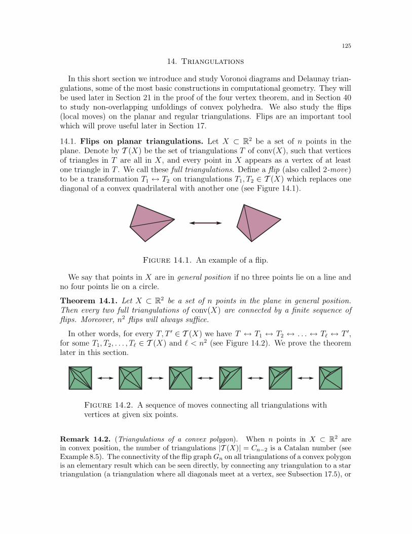
125

14. Triangulations

In this short section we introduce and study Voronoi diagrams and Delaunay trian-gulations, some of the most basic constructions in computational geometry. They willbe used later in Section 21 in the proof of the four vertex theorem, and in Section 40to study non-overlapping unfoldings of convex polyhedra. We also study the flips(local moves) on the planar and regular triangulations. Flips are an important toolwhich will prove useful later in Section 17.

14.1. Flips on planar triangulations. Let X ⊂ R2 be a set of n points in theplane. Denote by T (X) be the set of triangulations T of conv(X), such that verticesof triangles in T are all in X, and every point in X appears as a vertex of at leastone triangle in T . We call these full triangulations. Define a flip (also called 2-move)to be a transformation T1 ↔ T2 on triangulations T1, T2 ∈ T (X) which replaces onediagonal of a convex quadrilateral with another one (see Figure 14.1).

Figure 14.1. An example of a flip.

We say that points in X are in general position if no three points lie on a line andno four points lie on a circle.

Theorem 14.1. Let X ⊂ R2 be a set of n points in the plane in general position.Then every two full triangulations of conv(X) are connected by a finite sequence offlips. Moreover, n2 flips will always suffice.

In other words, for every T, T ′ ∈ T (X) we have T ↔ T1 ↔ T2 ↔ . . . ↔ Tℓ ↔ T ′,for some T1, T2, . . . , Tℓ ∈ T (X) and ℓ < n2 (see Figure 14.2). We prove the theoremlater in this section.

Figure 14.2. A sequence of moves connecting all triangulations withvertices at given six points.

Remark 14.2. (Triangulations of a convex polygon). When n points in X ⊂ R2 arein convex position, the number of triangulations |T (X)| = Cn−2 is a Catalan number (seeExample 8.5). The connectivity of the flip graphGn on all triangulations of a convex polygonis an elementary result which can be seen directly, by connecting any triangulation to a startriangulation (a triangulation where all diagonals meet at a vertex, see Subsection 17.5), or

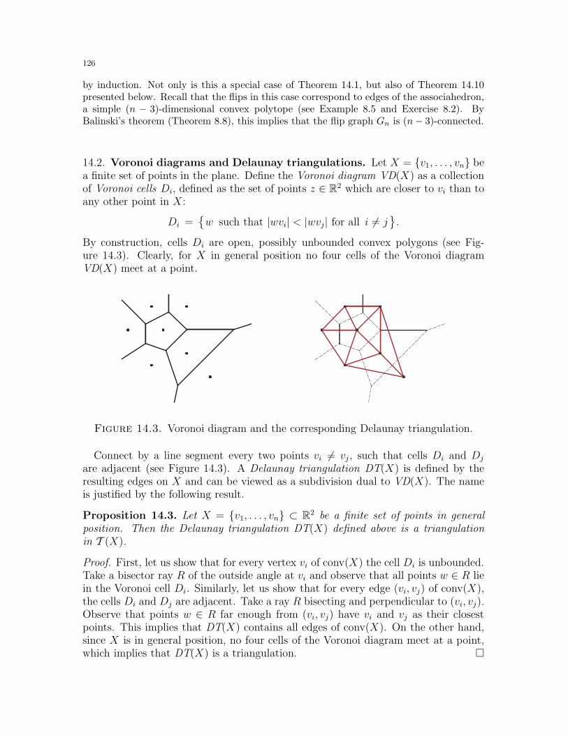
126

by induction. Not only is this a special case of Theorem 14.1, but also of Theorem 14.10presented below. Recall that the flips in this case correspond to edges of the associahedron,a simple (n − 3)-dimensional convex polytope (see Example 8.5 and Exercise 8.2). ByBalinski’s theorem (Theorem 8.8), this implies that the flip graph Gn is (n− 3)-connected.

14.2. Voronoi diagrams and Delaunay triangulations. Let X = v1, . . . , vn bea finite set of points in the plane. Define the Voronoi diagram VD(X) as a collectionof Voronoi cells Di, defined as the set of points z ∈ R2 which are closer to vi than toany other point in X:

Di =w such that |wvi| < |wvj| for all i 6= j

.

By construction, cells Di are open, possibly unbounded convex polygons (see Fig-ure 14.3). Clearly, for X in general position no four cells of the Voronoi diagramVD(X) meet at a point.

Figure 14.3. Voronoi diagram and the corresponding Delaunay triangulation.

Connect by a line segment every two points vi 6= vj , such that cells Di and Dj

are adjacent (see Figure 14.3). A Delaunay triangulation DT(X) is defined by theresulting edges on X and can be viewed as a subdivision dual to VD(X). The nameis justified by the following result.

Proposition 14.3. Let X = v1, . . . , vn ⊂ R2 be a finite set of points in generalposition. Then the Delaunay triangulation DT(X) defined above is a triangulationin T (X).

Proof. First, let us show that for every vertex vi of conv(X) the cell Di is unbounded.Take a bisector ray R of the outside angle at vi and observe that all points w ∈ R liein the Voronoi cell Di. Similarly, let us show that for every edge (vi, vj) of conv(X),the cells Di and Dj are adjacent. Take a ray R bisecting and perpendicular to (vi, vj).Observe that points w ∈ R far enough from (vi, vj) have vi and vj as their closestpoints. This implies that DT(X) contains all edges of conv(X). On the other hand,since X is in general position, no four cells of the Voronoi diagram meet at a point,which implies that DT(X) is a triangulation.

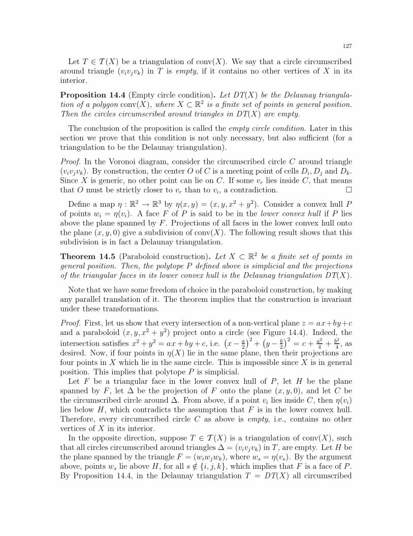
127

Let T ∈ T (X) be a triangulation of conv(X). We say that a circle circumscribedaround triangle (vivjvk) in T is empty, if it contains no other vertices of X in itsinterior.

Proposition 14.4 (Empty circle condition). Let DT(X) be the Delaunay triangula-tion of a polygon conv(X), where X ⊂ R2 is a finite set of points in general position.Then the circles circumscribed around triangles in DT(X) are empty.

The conclusion of the proposition is called the empty circle condition. Later in thissection we prove that this condition is not only necessary, but also sufficient (for atriangulation to be the Delaunay triangulation).

Proof. In the Voronoi diagram, consider the circumscribed circle C around triangle(vivjvk). By construction, the center O of C is a meeting point of cells Di, Dj and Dk.Since X is generic, no other point can lie on C. If some vr lies inside C, that meansthat O must be strictly closer to vr than to vi, a contradiction.

Define a map η : R2 → R3 by η(x, y) = (x, y, x2 + y2). Consider a convex hull Pof points wi = η(vi). A face F of P is said to be in the lower convex hull if P liesabove the plane spanned by F . Projections of all faces in the lower convex hull ontothe plane (x, y, 0) give a subdivision of conv(X). The following result shows that thissubdivision is in fact a Delaunay triangulation.

Theorem 14.5 (Paraboloid construction). Let X ⊂ R2 be a finite set of points ingeneral position. Then, the polytope P defined above is simplicial and the projectionsof the triangular faces in its lower convex hull is the Delaunay triangulation DT(X).

Note that we have some freedom of choice in the paraboloid construction, by makingany parallel translation of it. The theorem implies that the construction is invariantunder these transformations.

Proof. First, let us show that every intersection of a non-vertical plane z = ax+by+cand a paraboloid (x, y, x2 + y2) project onto a circle (see Figure 14.4). Indeed, the

intersection satisfies x2 + y2 = ax+ by+ c, i.e.(x− a

2

)2+(y− b

2

)2= c + a2

4+ b2

4, as

desired. Now, if four points in η(X) lie in the same plane, then their projections arefour points in X which lie in the same circle. This is impossible since X is in generalposition. This implies that polytope P is simplicial.

Let F be a triangular face in the lower convex hull of P , let H be the planespanned by F , let ∆ be the projection of F onto the plane (x, y, 0), and let C bethe circumscribed circle around ∆. From above, if a point vi lies inside C, then η(vi)lies below H , which contradicts the assumption that F is in the lower convex hull.Therefore, every circumscribed circle C as above is empty, i.e., contains no othervertices of X in its interior.

In the opposite direction, suppose T ∈ T (X) is a triangulation of conv(X), suchthat all circles circumscribed around triangles ∆ = (vivjvk) in T , are empty. Let H bethe plane spanned by the triangle F = (wiwjwk), where ws = η(vs). By the argumentabove, points ws lie above H , for all s /∈ i, j, k, which implies that F is a face of P .By Proposition 14.4, in the Delaunay triangulation T = DT(X) all circumscribed

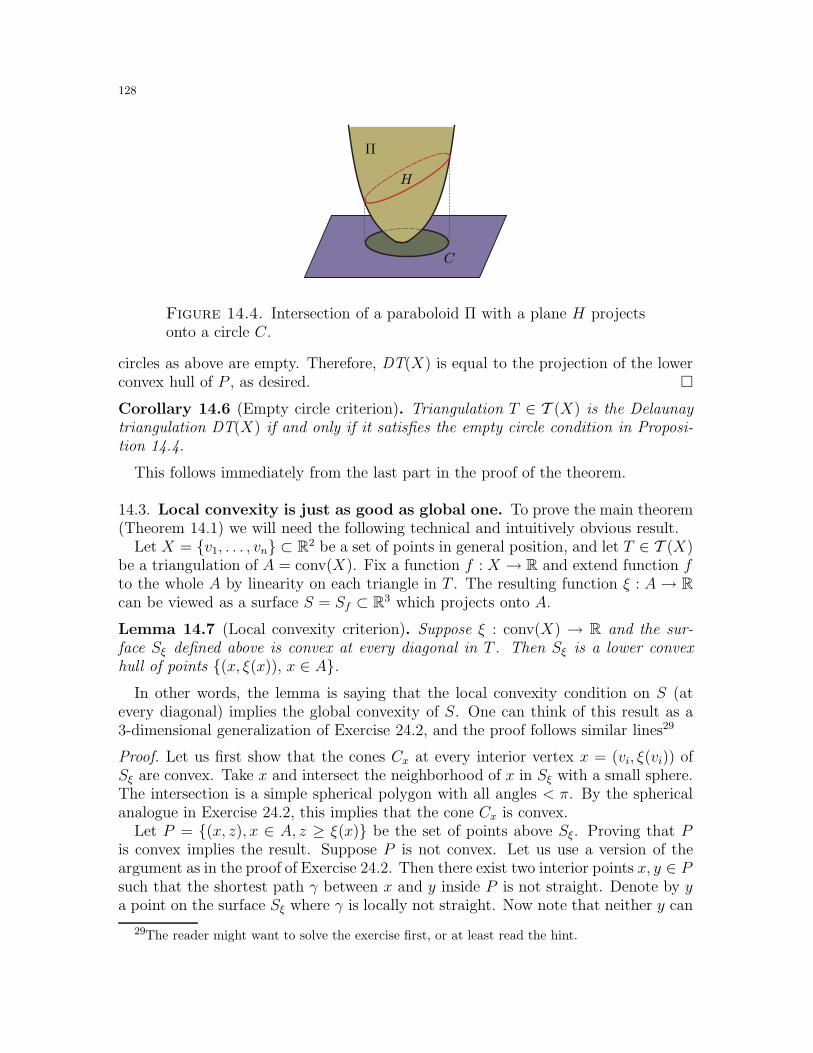
128

H

Π

C

Figure 14.4. Intersection of a paraboloid Π with a plane H projectsonto a circle C.

circles as above are empty. Therefore, DT(X) is equal to the projection of the lowerconvex hull of P , as desired.

Corollary 14.6 (Empty circle criterion). Triangulation T ∈ T (X) is the Delaunaytriangulation DT(X) if and only if it satisfies the empty circle condition in Proposi-tion 14.4.

This follows immediately from the last part in the proof of the theorem.

14.3. Local convexity is just as good as global one. To prove the main theorem(Theorem 14.1) we will need the following technical and intuitively obvious result.

Let X = v1, . . . , vn ⊂ R2 be a set of points in general position, and let T ∈ T (X)be a triangulation of A = conv(X). Fix a function f : X → R and extend function fto the whole A by linearity on each triangle in T . The resulting function ξ : A→ Rcan be viewed as a surface S = Sf ⊂ R3 which projects onto A.

Lemma 14.7 (Local convexity criterion). Suppose ξ : conv(X) → R and the sur-face Sξ defined above is convex at every diagonal in T . Then Sξ is a lower convexhull of points (x, ξ(x)), x ∈ A.

In other words, the lemma is saying that the local convexity condition on S (atevery diagonal) implies the global convexity of S. One can think of this result as a3-dimensional generalization of Exercise 24.2, and the proof follows similar lines29

Proof. Let us first show that the cones Cx at every interior vertex x = (vi, ξ(vi)) ofSξ are convex. Take x and intersect the neighborhood of x in Sξ with a small sphere.The intersection is a simple spherical polygon with all angles < π. By the sphericalanalogue in Exercise 24.2, this implies that the cone Cx is convex.

Let P = (x, z), x ∈ A, z ≥ ξ(x) be the set of points above Sξ. Proving that Pis convex implies the result. Suppose P is not convex. Let us use a version of theargument as in the proof of Exercise 24.2. Then there exist two interior points x, y ∈ Psuch that the shortest path γ between x and y inside P is not straight. Denote by ya point on the surface Sξ where γ is locally not straight. Now note that neither y can

29The reader might want to solve the exercise first, or at least read the hint.

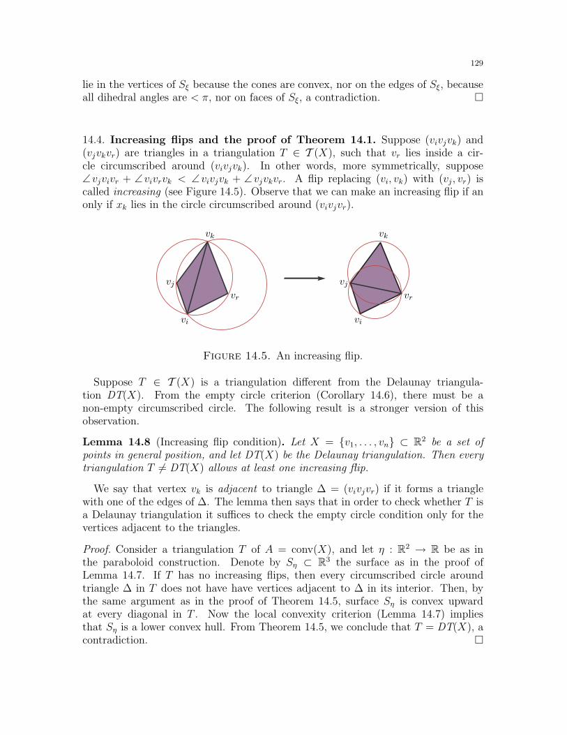
129

lie in the vertices of Sξ because the cones are convex, nor on the edges of Sξ, becauseall dihedral angles are < π, nor on faces of Sξ, a contradiction.

14.4. Increasing flips and the proof of Theorem 14.1. Suppose (vivjvk) and(vjvkvr) are triangles in a triangulation T ∈ T (X), such that vr lies inside a cir-cle circumscribed around (vivjvk). In other words, more symmetrically, suppose∠vjvivr + ∠vivrvk < ∠vivjvk + ∠vjvkvr. A flip replacing (vi, vk) with (vj , vr) iscalled increasing (see Figure 14.5). Observe that we can make an increasing flip if anonly if xk lies in the circle circumscribed around (vivjvr).

vjvj

vkvk

vrvr

vivi

Figure 14.5. An increasing flip.

Suppose T ∈ T (X) is a triangulation different from the Delaunay triangula-tion DT(X). From the empty circle criterion (Corollary 14.6), there must be anon-empty circumscribed circle. The following result is a stronger version of thisobservation.

Lemma 14.8 (Increasing flip condition). Let X = v1, . . . , vn ⊂ R2 be a set ofpoints in general position, and let DT(X) be the Delaunay triangulation. Then everytriangulation T 6= DT(X) allows at least one increasing flip.

We say that vertex vk is adjacent to triangle ∆ = (vivjvr) if it forms a trianglewith one of the edges of ∆. The lemma then says that in order to check whether T isa Delaunay triangulation it suffices to check the empty circle condition only for thevertices adjacent to the triangles.

Proof. Consider a triangulation T of A = conv(X), and let η : R2 → R be as inthe paraboloid construction. Denote by Sη ⊂ R3 the surface as in the proof ofLemma 14.7. If T has no increasing flips, then every circumscribed circle aroundtriangle ∆ in T does not have have vertices adjacent to ∆ in its interior. Then, bythe same argument as in the proof of Theorem 14.5, surface Sη is convex upwardat every diagonal in T . Now the local convexity criterion (Lemma 14.7) impliesthat Sη is a lower convex hull. From Theorem 14.5, we conclude that T = DT(X), acontradiction.

130

Proof of Theorem 14.1. Fix a triangulation T ∈ T (X). We will show that startingwith T , after at most

(n2

)increasing flips, we can always obtain DT(X). This implies

that every two triangulations are connected by at most 2(n2

)< n2 flips.

Let S = Sη be the surface defined as above. Suppose there exists an increasing flipT → T ′, replacing some (vj , vk) with some (vivr). Observe that the resulting surfaceS ′ lies directly below S, and, in particular, below the edge (vj, vk). Continue makingincreasing flips. From above, the edges of the flips are never repeated, and after atmost

(n2

)flips we obtain a triangulation without increasing flips. By the lemma, this

must be the Delaunay triangulation DT(X).

Remark 14.9. (Delaunay triangulations in higher dimensions). For a set of points X ⊂Rd, d ≥ 3, the definitions of Voronoi diagram and Delaunay triangulations extend nearlyverbatim (see Exercise 14.2). The same goes for the empty sphere criterion (Corollary 14.6and the Delaunay triangulation construction (Theorem 14.5).

Unfortunately, the increasing flips argument (Lemma 14.8) does not hold in full generality.Figuring out what goes wrong is difficult to see at first. That is because the intuitivelyobvious local convexity criterion no longer holds (see Exercise 14.3). In fact, the analogueof Theorem 14.1 is an open problem for triangulations of convex polytopes in R3. It failsfor general sets X ⊂ R3 (that are not necessarily in convex position), and for convex X inhigher dimensions (see Subsection 14.7).

14.5. Regular triangulations. While a direct generalization of Theorem 14.1 failsfor triangulations in higher dimensions (see Remark 14.9 and Subsection 14.7), choos-ing a nice subset of triangulations is still connected by flips. The following variationon Theorem14.1 will prove useful in Section 17.

Let P ⊂ Rd be a simplicial convex polytope and let V be the set of its vertices. Wesay that P is generic if no d+ 1 vertices lie in the same hyperplane. A triangulationof P is a full triangulation with vertices in V . By a slight change of notation, denoteT (P ) the set of all triangulations of P ; these triangulations are exactly full triangu-lations on the set of vertices V . For the rest of this section, we will consider only fulltriangulations of polytopes.

For every function ξ : V → R, let Sξ be the lower convex hull surface of points(v, ξ(v)

)inRd+1 defined as above. The last coordinate of a point (x, ξ) ∈ S is called

the height of x ∈ P , and the function ξ is called the height function.Observe that the projection of Sξ onto P gives a polyhedral subdivision Qξ of P

(see Figure 14.6). We call Qξ the subdivision associated with the function ξ. We saythat ξ is generic if no d + 2 vertices of Sξ lie in the same hyperplane in Rd+1. Notethat when ξ is generic, Qξ is a full triangulation: Qξ ∈ T (P ).

A full triangulation T ∈ T (P ) is called regular if there exists a height function ξ,such that T = Qξ is a triangulation associated with ξ. Denote by T∗(P ) the set ofall regular triangulations T ∈ T (P ). For example, by the paraboloid construction(Theorem 14.5), the Delaunay triangulation of a convex polygon is always regular.In fact, part a) of Exercise 14.10 says that every triangulation of a convex polygon isregular.

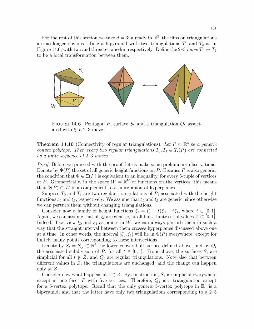
131

For the rest of this section we take d = 3; already in R3, the flips on triangulationsare no longer obvious. Take a bipyramid with two triangulations T1 and T2 as inFigure 14.6, with two and three tetrahedra, respectively. Define the 2–3 move T1 ↔ T2

to be a local transformation between them.

PQξ

Sξ

Figure 14.6. Pentagon P , surface Sξ and a triangulation Qξ associ-ated with ξ; a 2–3 move.

Theorem 14.10 (Connectivity of regular triangulations). Let P ⊂ R3 be a genericconvex polytope. Then every two regular triangulations T0, T1 ∈ T∗(P ) are connectedby a finite sequence of 2–3 moves.

Proof. Before we proceed with the proof, let us make some preliminary observations.Denote by Φ(P ) the set of all generic height functions on P . Because P is also generic,the condition that Φ ∈ Ξ(P ) is equivalent to an inequality, for every 5-tuple of verticesof P . Geometrically, in the space W = RV of functions on the vertices, this meansthat Φ(P ) ⊂W is a complement to a finite union of hyperplanes.

Suppose T0 and T1 are two regular triangulations of P , associated with the heightfunctions ξ0 and ξ1, respectively. We assume that ξ0 and ξ1 are generic, since otherwisewe can perturb them without changing triangulations.

Consider now a family of height functions ξt = (1 − t)ξ0 + tξ1, where t ∈ [0, 1].Again, we can assume that all ξt are generic, at all but a finite set of values Z ⊂ [0, 1].Indeed, if we view ξ0 and ξ1 as points in W , we can always perturb them in such away that the straight interval between them crosses hyperplanes discussed above oneat a time. In other words, the interval [ξ0, ξ1] will lie in Φ(P ) everywhere, except forfinitely many points corresponding to these intersections.

Denote by St = Sξt ⊂ R4 the lower convex hull surface defined above, and by Qt

the associated subdivision of P , for all t ∈ [0, 1]. From above, the surfaces St aresimplicial for all t /∈ Z, and Qt are regular triangulations. Note also that betweendifferent values in Z, the triangulations are unchanged, and the change can happenonly at Z.

Consider now what happens at z ∈ Z. By construction, Sz is simplicial everywhereexcept at one facet F with five vertices. Therefore, Qz is a triangulation exceptfor a 5-vertex polytope. Recall that the only generic 5-vertex polytope in R3 is abipyramid, and that the latter have only two triangulations corresponding to a 2–3

132

move. Therefore, by continuity, we conclude that Qt where t → z−, and Qt wheret → z+, correspond to two triangulations which differ by a 2–3 move. Since Z isfinite, this implies that there is a finite sequence of 2–3 moves corresponding to allz ∈ Z, which connects T0 and T1.

14.6. Exercises.

Exercise 14.1. ♦ a) [1] State precisely what generality assumption need to be used on ξ0and ξ1 in the proof of Theorem 14.10.b) [1] Suppose polytope P ⊂ R3 has n vertices. Give a polynomial upper bound on thenumber of 2–3 moves between any two full triangulations of P .c) [1] Generalize Theorem 14.10 to higher dimensions.

Exercise 14.2. (Delaunay triangulations in higher dimensions) ♦ Define the Voronoidiagram and Delaunay triangulation of a finite sets of points X ⊂ Rd in general position,d ≥ 1.a) [1] Prove the empty sphere criterion, a generalization of Proposition 14.4 to all d ≥ 1.b) [1+] Generalize Theorem 14.5 to all d ≥ 1.

Exercise 14.3. (Local convexity criterion in R4) ♦ [1+] Find a set X ⊂ R3, a triangulationof A = conv(X), and a function f : R3 → R, such that the local convexity criterion fails onSf ⊂ R4, i.e., show that Sf can be convex at all 2-faces, but not globally convex.

Exercise 14.4. (Inverse Voronoi diagrams and inverse Delaunay triangulations) ♦ LetX ⊂ R2 be a finite set of points in general position. Subdivide the plane into cells accordingto the furthest point in X. For this inverse Voronoi diagram define the correspondinginverse Delaunay triangulation IDT(X).a) [1] Prove the full circle condition, the analogue of Proposition 14.4.b) [1] Give a paraboloid style construction of IDT(X), the analogue of Theorem 14.5.c) [1] Define decreasing flips to be the inverse of increasing flips. Prove that every triangu-lation T ∈ T (X) is connected to IDT(X) by at most

(n2

)decreasing flips.

Exercise 14.5. (Double chain configuration) ♦ a) [1] Let Xn ⊂ R2 be the set of n = 2kpoints as in Figure 14.7. Prove that the edges as in the figure must be present in every fulltriangulation of conv(Xn). Conclude that the number of full triangulations is equal to

|T (Xn)| =

(2k − 2

k − 1

)C2k−2 ,

where Cn = 1n+1

(2nn

)is the Catalan number (see Example 8.5).

b) [1+] Prove that the diameter of the flip graph on T (Xn) is Ω(n2).

Exercise 14.6. [1] Let T be a full triangulation of a convex n-gon with k interior pointsx1, . . . , xi. Suppose every interior point xi is adjacent to at least 6 triangles in T . Provethat k = O(n2).

Exercise 14.7. (Number of planar triangulations) a) [2-] Prove that for every X ⊂ R2 in

general position, the number of full triangulations is at least exponential: |T (X)| = eΩ(n).b) [2] Prove that for every X ⊂ R2, the number of full triangulations is at most exponential:

|T (X)| = eO(n).

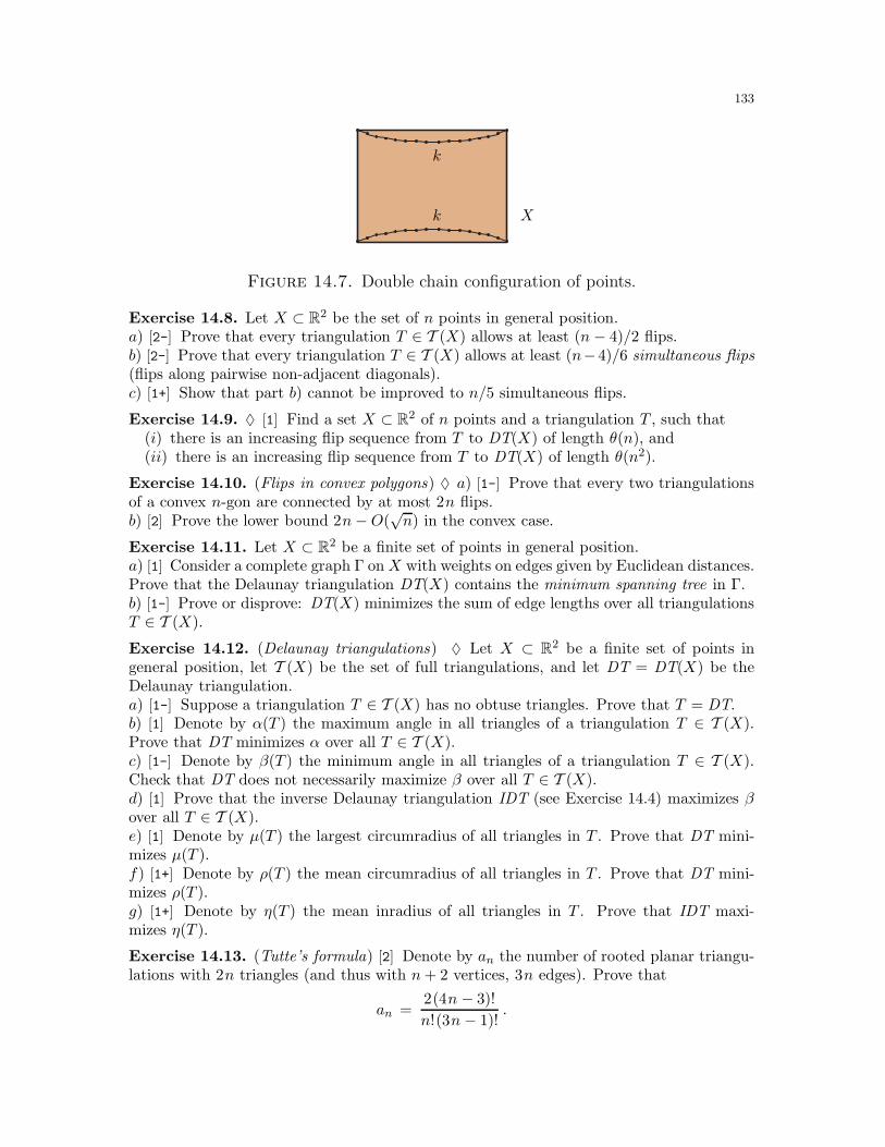
133

k

k

X

Figure 14.7. Double chain configuration of points.

Exercise 14.8. Let X ⊂ R2 be the set of n points in general position.a) [2-] Prove that every triangulation T ∈ T (X) allows at least (n − 4)/2 flips.b) [2-] Prove that every triangulation T ∈ T (X) allows at least (n−4)/6 simultaneous flips(flips along pairwise non-adjacent diagonals).c) [1+] Show that part b) cannot be improved to n/5 simultaneous flips.

Exercise 14.9. ♦ [1] Find a set X ⊂ R2 of n points and a triangulation T , such that(i) there is an increasing flip sequence from T to DT(X) of length θ(n), and(ii) there is an increasing flip sequence from T to DT(X) of length θ(n2).

Exercise 14.10. (Flips in convex polygons) ♦ a) [1-] Prove that every two triangulationsof a convex n-gon are connected by at most 2n flips.b) [2] Prove the lower bound 2n−O(

√n) in the convex case.

Exercise 14.11. Let X ⊂ R2 be a finite set of points in general position.a) [1] Consider a complete graph Γ on X with weights on edges given by Euclidean distances.Prove that the Delaunay triangulation DT(X) contains the minimum spanning tree in Γ.b) [1-] Prove or disprove: DT(X) minimizes the sum of edge lengths over all triangulationsT ∈ T (X).

Exercise 14.12. (Delaunay triangulations) ♦ Let X ⊂ R2 be a finite set of points ingeneral position, let T (X) be the set of full triangulations, and let DT = DT(X) be theDelaunay triangulation.a) [1-] Suppose a triangulation T ∈ T (X) has no obtuse triangles. Prove that T = DT.b) [1] Denote by α(T ) the maximum angle in all triangles of a triangulation T ∈ T (X).Prove that DT minimizes α over all T ∈ T (X).c) [1-] Denote by β(T ) the minimum angle in all triangles of a triangulation T ∈ T (X).Check that DT does not necessarily maximize β over all T ∈ T (X).d) [1] Prove that the inverse Delaunay triangulation IDT (see Exercise 14.4) maximizes βover all T ∈ T (X).e) [1] Denote by µ(T ) the largest circumradius of all triangles in T . Prove that DT mini-mizes µ(T ).f) [1+] Denote by ρ(T ) the mean circumradius of all triangles in T . Prove that DT mini-mizes ρ(T ).g) [1+] Denote by η(T ) the mean inradius of all triangles in T . Prove that IDT maxi-mizes η(T ).

Exercise 14.13. (Tutte’s formula) [2] Denote by an the number of rooted planar triangu-lations with 2n triangles (and thus with n+ 2 vertices, 3n edges). Prove that

an =2(4n − 3)!

n!(3n − 1)!.

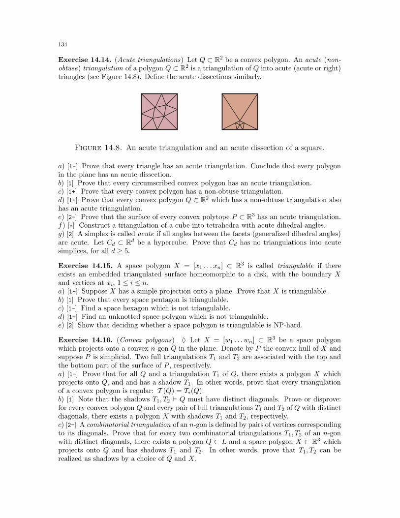
134

Exercise 14.14. (Acute triangulations) Let Q ⊂ R2 be a convex polygon. An acute (non-obtuse) triangulation of a polygon Q ⊂ R2 is a triangulation of Q into acute (acute or right)triangles (see Figure 14.8). Define the acute dissections similarly.

Figure 14.8. An acute triangulation and an acute dissection of a square.

a) [1-] Prove that every triangle has an acute triangulation. Conclude that every polygonin the plane has an acute dissection.b) [1] Prove that every circumscribed convex polygon has an acute triangulation.c) [1+] Prove that every convex polygon has a non-obtuse triangulation.d) [1+] Prove that every convex polygon Q ⊂ R2 which has a non-obtuse triangulation alsohas an acute triangulation.e) [2-] Prove that the surface of every convex polytope P ⊂ R3 has an acute triangulation.f) [∗] Construct a triangulation of a cube into tetrahedra with acute dihedral angles.g) [2] A simplex is called acute if all angles between the facets (generalized dihedral angles)are acute. Let Cd ⊂ Rd be a hypercube. Prove that Cd has no triangulations into acutesimplices, for all d ≥ 5.

Exercise 14.15. A space polygon X = [x1 . . . xn] ⊂ R3 is called triangulable if thereexists an embedded triangulated surface homeomorphic to a disk, with the boundary Xand vertices at xi, 1 ≤ i ≤ n.a) [1-] Suppose X has a simple projection onto a plane. Prove that X is triangulable.b) [1] Prove that every space pentagon is triangulable.c) [1-] Find a space hexagon which is not triangulable.d) [1+] Find an unknotted space polygon which is not triangulable.e) [2] Show that deciding whether a space polygon is triangulable is NP-hard.

Exercise 14.16. (Convex polygons) ♦ Let X = [w1 . . . wn] ⊂ R3 be a space polygonwhich projects onto a convex n-gon Q in the plane. Denote by P the convex hull of X andsuppose P is simplicial. Two full triangulations T1 and T2 are associated with the top andthe bottom part of the surface of P , respectively.a) [1-] Prove that for all Q and a triangulation T1 of Q, there exists a polygon X whichprojects onto Q, and and has a shadow T1. In other words, prove that every triangulationof a convex polygon is regular: T (Q) = T∗(Q).b) [1] Note that the shadows T1, T2 ⊢ Q must have distinct diagonals. Prove or disprove:for every convex polygon Q and every pair of full triangulations T1 and T2 of Q with distinctdiagonals, there exists a polygon X with shadows T1 and T2, respectively.c) [2-] A combinatorial triangulation of an n-gon is defined by pairs of vertices correspondingto its diagonals. Prove that for every two combinatorial triangulations T1, T2 of an n-gonwith distinct diagonals, there exists a polygon Q ⊂ L and a space polygon X ⊂ R3 whichprojects onto Q and has shadows T1 and T2. In other words, prove that T1, T2 can berealized as shadows by a choice of Q and X.

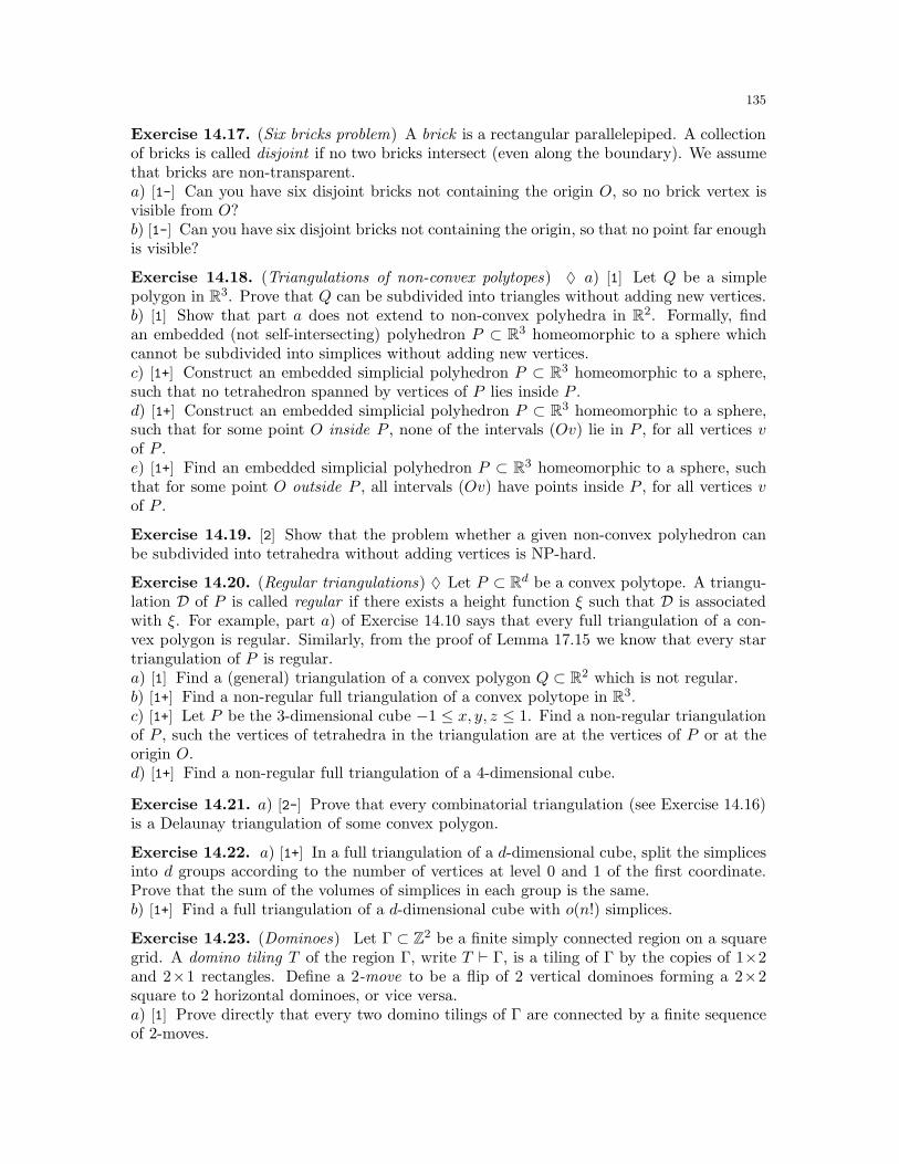
135

Exercise 14.17. (Six bricks problem) A brick is a rectangular parallelepiped. A collectionof bricks is called disjoint if no two bricks intersect (even along the boundary). We assumethat bricks are non-transparent.a) [1-] Can you have six disjoint bricks not containing the origin O, so no brick vertex isvisible from O?b) [1-] Can you have six disjoint bricks not containing the origin, so that no point far enoughis visible?

Exercise 14.18. (Triangulations of non-convex polytopes) ♦ a) [1] Let Q be a simplepolygon in R3. Prove that Q can be subdivided into triangles without adding new vertices.b) [1] Show that part a does not extend to non-convex polyhedra in R2. Formally, findan embedded (not self-intersecting) polyhedron P ⊂ R3 homeomorphic to a sphere whichcannot be subdivided into simplices without adding new vertices.c) [1+] Construct an embedded simplicial polyhedron P ⊂ R3 homeomorphic to a sphere,such that no tetrahedron spanned by vertices of P lies inside P .d) [1+] Construct an embedded simplicial polyhedron P ⊂ R3 homeomorphic to a sphere,such that for some point O inside P , none of the intervals (Ov) lie in P , for all vertices vof P .e) [1+] Find an embedded simplicial polyhedron P ⊂ R3 homeomorphic to a sphere, suchthat for some point O outside P , all intervals (Ov) have points inside P , for all vertices vof P .

Exercise 14.19. [2] Show that the problem whether a given non-convex polyhedron canbe subdivided into tetrahedra without adding vertices is NP-hard.

Exercise 14.20. (Regular triangulations) ♦ Let P ⊂ Rd be a convex polytope. A triangu-lation D of P is called regular if there exists a height function ξ such that D is associatedwith ξ. For example, part a) of Exercise 14.10 says that every full triangulation of a con-vex polygon is regular. Similarly, from the proof of Lemma 17.15 we know that every startriangulation of P is regular.a) [1] Find a (general) triangulation of a convex polygon Q ⊂ R2 which is not regular.b) [1+] Find a non-regular full triangulation of a convex polytope in R3.c) [1+] Let P be the 3-dimensional cube −1 ≤ x, y, z ≤ 1. Find a non-regular triangulationof P , such the vertices of tetrahedra in the triangulation are at the vertices of P or at theorigin O.d) [1+] Find a non-regular full triangulation of a 4-dimensional cube.

Exercise 14.21. a) [2-] Prove that every combinatorial triangulation (see Exercise 14.16)is a Delaunay triangulation of some convex polygon.

Exercise 14.22. a) [1+] In a full triangulation of a d-dimensional cube, split the simplicesinto d groups according to the number of vertices at level 0 and 1 of the first coordinate.Prove that the sum of the volumes of simplices in each group is the same.b) [1+] Find a full triangulation of a d-dimensional cube with o(n!) simplices.

Exercise 14.23. (Dominoes) Let Γ ⊂ Z2 be a finite simply connected region on a squaregrid. A domino tiling T of the region Γ, write T ⊢ Γ, is a tiling of Γ by the copies of 1×2and 2×1 rectangles. Define a 2-move to be a flip of 2 vertical dominoes forming a 2×2square to 2 horizontal dominoes, or vice versa.a) [1] Prove directly that every two domino tilings of Γ are connected by a finite sequenceof 2-moves.

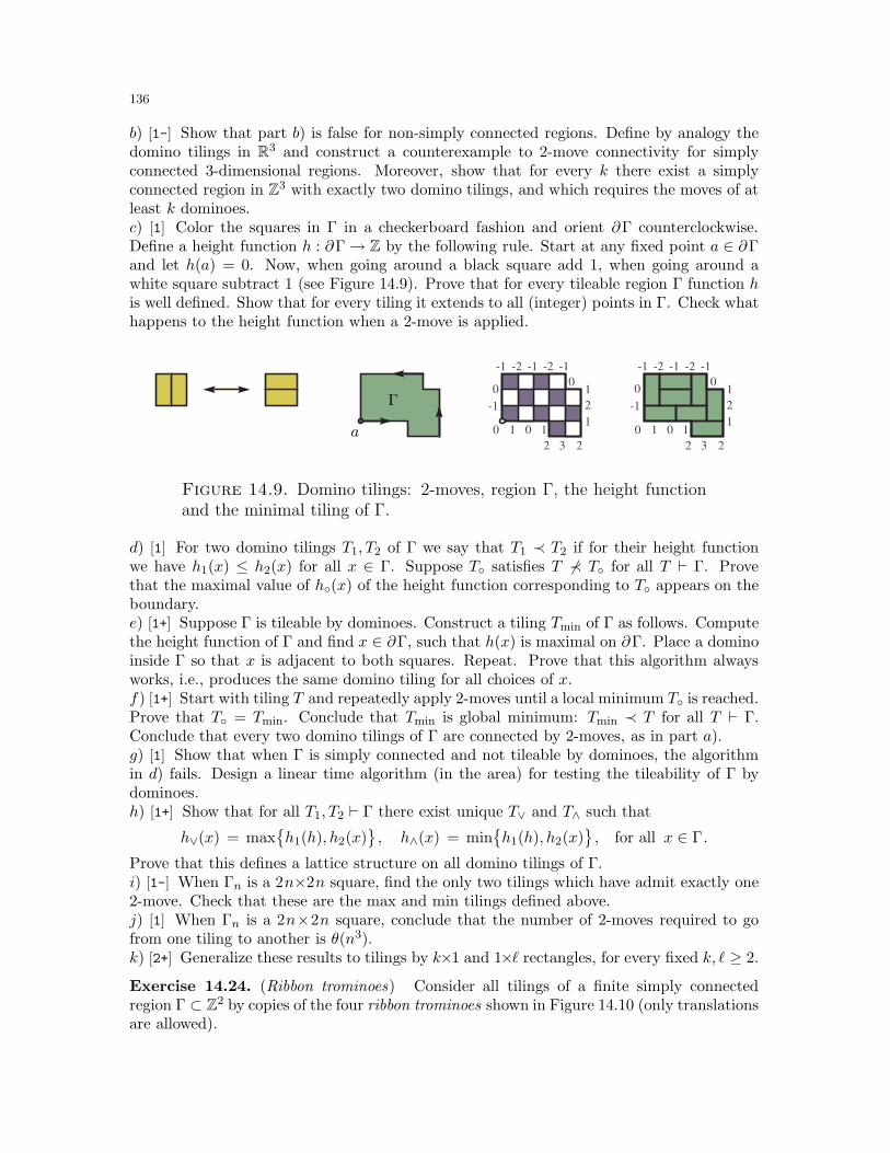
136

b) [1-] Show that part b) is false for non-simply connected regions. Define by analogy thedomino tilings in R3 and construct a counterexample to 2-move connectivity for simplyconnected 3-dimensional regions. Moreover, show that for every k there exist a simplyconnected region in Z3 with exactly two domino tilings, and which requires the moves of atleast k dominoes.c) [1] Color the squares in Γ in a checkerboard fashion and orient ∂Γ counterclockwise.Define a height function h : ∂Γ→ Z by the following rule. Start at any fixed point a ∈ ∂Γand let h(a) = 0. Now, when going around a black square add 1, when going around awhite square subtract 1 (see Figure 14.9). Prove that for every tileable region Γ function his well defined. Show that for every tiling it extends to all (integer) points in Γ. Check whathappens to the height function when a 2-move is applied.

01

0 1

2 3 2

1

1

2

-1

0

-2-1-2-1

0

-1

01

0 1

2 3 2

1

1

2

-1

0

-2-1-2-1

0

-1Γ

a

Figure 14.9. Domino tilings: 2-moves, region Γ, the height functionand the minimal tiling of Γ.

d) [1] For two domino tilings T1, T2 of Γ we say that T1 ≺ T2 if for their height functionwe have h1(x) ≤ h2(x) for all x ∈ Γ. Suppose T satisfies T ⊀ T for all T ⊢ Γ. Provethat the maximal value of h(x) of the height function corresponding to T appears on theboundary.e) [1+] Suppose Γ is tileable by dominoes. Construct a tiling Tmin of Γ as follows. Computethe height function of Γ and find x ∈ ∂Γ, such that h(x) is maximal on ∂Γ. Place a dominoinside Γ so that x is adjacent to both squares. Repeat. Prove that this algorithm alwaysworks, i.e., produces the same domino tiling for all choices of x.f) [1+] Start with tiling T and repeatedly apply 2-moves until a local minimum T is reached.Prove that T = Tmin. Conclude that Tmin is global minimum: Tmin ≺ T for all T ⊢ Γ.Conclude that every two domino tilings of Γ are connected by 2-moves, as in part a).g) [1] Show that when Γ is simply connected and not tileable by dominoes, the algorithmin d) fails. Design a linear time algorithm (in the area) for testing the tileability of Γ bydominoes.h) [1+] Show that for all T1, T2 ⊢ Γ there exist unique T∨ and T∧ such that

h∨(x) = maxh1(h), h2(x)

, h∧(x) = min

h1(h), h2(x)

, for all x ∈ Γ.

Prove that this defines a lattice structure on all domino tilings of Γ.i) [1-] When Γn is a 2n×2n square, find the only two tilings which have admit exactly one2-move. Check that these are the max and min tilings defined above.j) [1] When Γn is a 2n×2n square, conclude that the number of 2-moves required to gofrom one tiling to another is θ(n3).k) [2+] Generalize these results to tilings by k×1 and 1×ℓ rectangles, for every fixed k, ℓ ≥ 2.

Exercise 14.24. (Ribbon trominoes) Consider all tilings of a finite simply connectedregion Γ ⊂ Z2 by copies of the four ribbon trominoes shown in Figure 14.10 (only translationsare allowed).

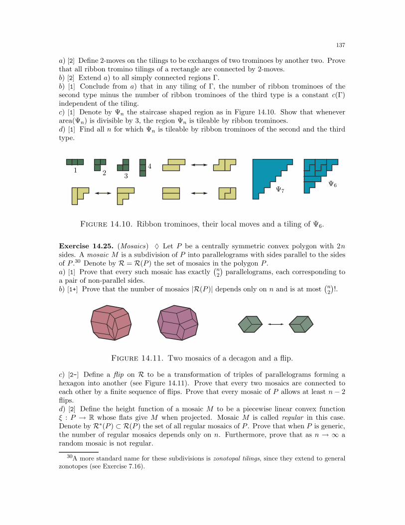
137

a) [2] Define 2-moves on the tilings to be exchanges of two trominoes by another two. Provethat all ribbon tromino tilings of a rectangle are connected by 2-moves.b) [2] Extend a) to all simply connected regions Γ.b) [1] Conclude from a) that in any tiling of Γ, the number of ribbon trominoes of thesecond type minus the number of ribbon trominoes of the third type is a constant c(Γ)independent of the tiling.c) [1] Denote by Ψn the staircase shaped region as in Figure 14.10. Show that wheneverarea(Ψn) is divisible by 3, the region Ψn is tileable by ribbon trominoes.d) [1] Find all n for which Ψn is tileable by ribbon trominoes of the second and the thirdtype.

1 2 3

4

Ψ7

Ψ6

Figure 14.10. Ribbon trominoes, their local moves and a tiling of Ψ6.

Exercise 14.25. (Mosaics) ♦ Let P be a centrally symmetric convex polygon with 2nsides. A mosaic M is a subdivision of P into parallelograms with sides parallel to the sidesof P .30 Denote by R = R(P ) the set of mosaics in the polygon P .a) [1] Prove that every such mosaic has exactly

(n2

)parallelograms, each corresponding to

a pair of non-parallel sides.b) [1+] Prove that the number of mosaics |R(P )| depends only on n and is at most

(n2

)!.

Figure 14.11. Two mosaics of a decagon and a flip.

c) [2-] Define a flip on R to be a transformation of triples of parallelograms forming ahexagon into another (see Figure 14.11). Prove that every two mosaics are connected toeach other by a finite sequence of flips. Prove that every mosaic of P allows at least n− 2flips.d) [2] Define the height function of a mosaic M to be a piecewise linear convex functionξ : P → R whose flats give M when projected. Mosaic M is called regular in this case.Denote by R∗(P ) ⊂ R(P ) the set of all regular mosaics of P . Prove that when P is generic,the number of regular mosaics depends only on n. Furthermore, prove that as n → ∞ arandom mosaic is not regular.

30A more standard name for these subdivisions is zonotopal tilings, since they extend to generalzonotopes (see Exercise 7.16).

138

e) [2-] When P is deformed, one can also deform a mosaic. Prove that there exists a mosaicwhich is not regular for all deformations.

Exercise 14.26. [1] Let P be a centrally symmetric convex polygon. Consider a subdivisionof P into finitely many centrally symmetric polygons. Use Exercise 2.3 to prove that thistiling has at least 3 parallelograms.

14.7. Final remarks. Voronoi diagrams are named after the Georgy Voronoy who intro-duced them in 1908. In a different context they were studied much earlier, most notably byDescartes (1644) and Dirichlet (1850). Similarly, Delaunay triangulations are named afterBoris Delone (note another difference in spelling), who proved the empty sphere criterion(Exercise 14.2) in 1934. According to Dolbilin, this result was repeatedly rediscovered in theWest, but after Coxeter received a letter from Delone, he read and popularized the originalpapers of Voronoy and Delone. For more on Voronoi diagrams and Delaunay triangulations,their history, applications and references see [Aur, AurK].

The inverse Voronoi diagrams (and dual to them inverse Delaunay triangulations) definedin Exercise 14.4, go back to the foundational paper [ShaH]. They are usually called the“furthest site” or the “farthest point” Voronoi diagrams [AurK].

The local convexity criterion (Lemma 14.7) is a discrete version of a classical result byHadamard (1897), further generalized by Tietze (1928), Nakajima (1928) and others. Werefer to [KarB] for further references.

The flip (local move) connectivity on full triangulations has been also extensively studiedin the literature [San2]. In particular, in dimension d ≥ 5 the flip graph can be disconnected,and there is an evidence that this might be true even for d = 3. For more on various classes oftriangulations, in particular regular triangulations, and connections to other fields see [DRS](see also [San2]).

The full triangulations (triangulations with a fixed set of vertices) have also been studiedat length in connection with A-discriminants and variations on the theme. The height func-tions and regular triangulations (see Exercise 14.20) play important roles in the field. Werefer the reader to [GKZ], where many of these fundamental results were first summarized(a number of connections and applications have appeared since [GKZ]).

Let us mention here the mosaics (zonotopal tilings) defined in Exercise 14.25. In a certainprecise sense, the regular mosaics are projections of the “top” 2-dimensional faces of ahypercube. In a different direction, the mosaics correspond to the pseudoline arrangements,while regular mosaics are dual to stretchable pseudoline arrangements. We refer to [Bjo+]for further results and references.

Finally, the local move connectivity plays an important role in the modern study of finite

tilings. In some special cases one can use the height functions and combinatorial group

theory to establish that certain local moves connect all tilings of a given region by a fixed

set of tiles. Some examples are given in Exercises 14.23 and 14.24. See [Pak3] for these and

other tiling results, and the references.

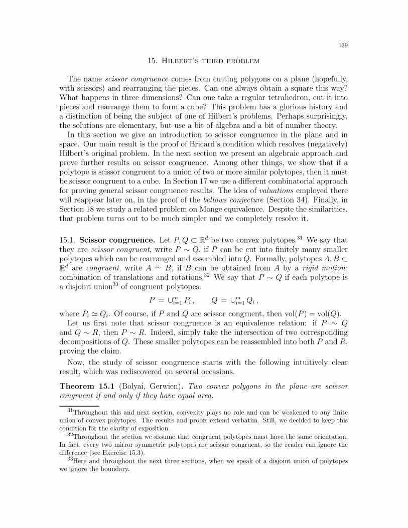
139

15. Hilbert’s third problem

The name scissor congruence comes from cutting polygons on a plane (hopefully,with scissors) and rearranging the pieces. Can one always obtain a square this way?What happens in three dimensions? Can one take a regular tetrahedron, cut it intopieces and rearrange them to form a cube? This problem has a glorious history anda distinction of being the subject of one of Hilbert’s problems. Perhaps surprisingly,the solutions are elementary, but use a bit of algebra and a bit of number theory.

In this section we give an introduction to scissor congruence in the plane and inspace. Our main result is the proof of Bricard’s condition which resolves (negatively)Hilbert’s original problem. In the next section we present an algebraic approach andprove further results on scissor congruence. Among other things, we show that if apolytope is scissor congruent to a union of two or more similar polytopes, then it mustbe scissor congruent to a cube. In Section 17 we use a different combinatorial approachfor proving general scissor congruence results. The idea of valuations employed therewill reappear later on, in the proof of the bellows conjecture (Section 34). Finally, inSection 18 we study a related problem on Monge equivalence. Despite the similarities,that problem turns out to be much simpler and we completely resolve it.

15.1. Scissor congruence. Let P,Q ⊂ Rd be two convex polytopes.31 We say thatthey are scissor congruent, write P ∼ Q, if P can be cut into finitely many smallerpolytopes which can be rearranged and assembled into Q. Formally, polytopes A,B ⊂Rd are congruent, write A ≃ B, if B can be obtained from A by a rigid motion:combination of translations and rotations.32 We say that P ∼ Q if each polytope isa disjoint union33 of congruent polytopes:

P = ∪mi=1 Pi , Q = ∪mi=1Qi ,

where Pi ≃ Qi. Of course, if P and Q are scissor congruent, then vol(P ) = vol(Q).Let us first note that scissor congruence is an equivalence relation: if P ∼ Q

and Q ∼ R, then P ∼ R. Indeed, simply take the intersection of two correspondingdecompositions of Q. These smaller polytopes can be reassembled into both P and R,proving the claim.

Now, the study of scissor congruence starts with the following intuitively clearresult, which was rediscovered on several occasions.

Theorem 15.1 (Bolyai, Gerwien). Two convex polygons in the plane are scissorcongruent if and only if they have equal area.

31Throughout this and next section, convexity plays no role and can be weakened to any finiteunion of convex polytopes. The results and proofs extend verbatim. Still, we decided to keep thiscondition for the clarity of exposition.

32Throughout the section we assume that congruent polytopes must have the same orientation.In fact, every two mirror symmetric polytopes are scissor congruent, so the reader can ignore thedifference (see Exercise 15.3).

33Here and throughout the next three sections, when we speak of a disjoint union of polytopeswe ignore the boundary.

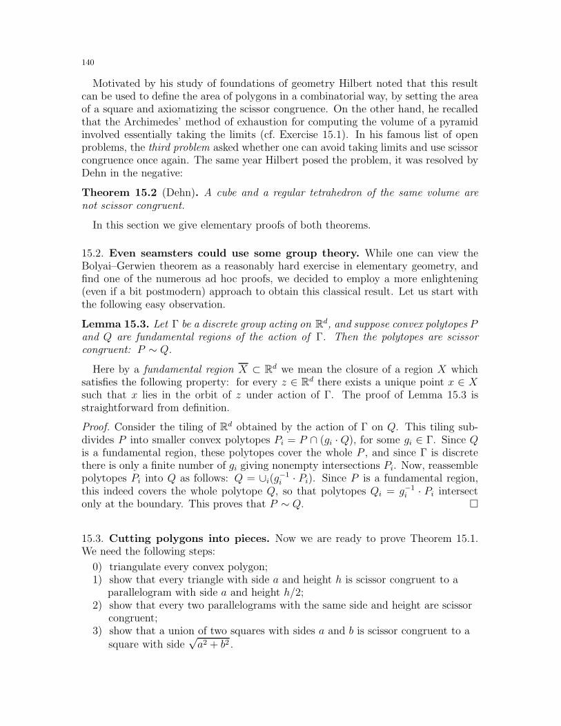
140

Motivated by his study of foundations of geometry Hilbert noted that this resultcan be used to define the area of polygons in a combinatorial way, by setting the areaof a square and axiomatizing the scissor congruence. On the other hand, he recalledthat the Archimedes’ method of exhaustion for computing the volume of a pyramidinvolved essentially taking the limits (cf. Exercise 15.1). In his famous list of openproblems, the third problem asked whether one can avoid taking limits and use scissorcongruence once again. The same year Hilbert posed the problem, it was resolved byDehn in the negative:

Theorem 15.2 (Dehn). A cube and a regular tetrahedron of the same volume arenot scissor congruent.

In this section we give elementary proofs of both theorems.

15.2. Even seamsters could use some group theory. While one can view theBolyai–Gerwien theorem as a reasonably hard exercise in elementary geometry, andfind one of the numerous ad hoc proofs, we decided to employ a more enlightening(even if a bit postmodern) approach to obtain this classical result. Let us start withthe following easy observation.

Lemma 15.3. Let Γ be a discrete group acting on Rd, and suppose convex polytopes Pand Q are fundamental regions of the action of Γ. Then the polytopes are scissorcongruent: P ∼ Q.

Here by a fundamental region X ⊂ Rd we mean the closure of a region X whichsatisfies the following property: for every z ∈ Rd there exists a unique point x ∈ Xsuch that x lies in the orbit of z under action of Γ. The proof of Lemma 15.3 isstraightforward from definition.

Proof. Consider the tiling of Rd obtained by the action of Γ on Q. This tiling sub-divides P into smaller convex polytopes Pi = P ∩ (gi · Q), for some gi ∈ Γ. Since Qis a fundamental region, these polytopes cover the whole P , and since Γ is discretethere is only a finite number of gi giving nonempty intersections Pi. Now, reassemblepolytopes Pi into Q as follows: Q = ∪i(g−1

i · Pi). Since P is a fundamental region,this indeed covers the whole polytope Q, so that polytopes Qi = g−1

i · Pi intersectonly at the boundary. This proves that P ∼ Q.

15.3. Cutting polygons into pieces. Now we are ready to prove Theorem 15.1.We need the following steps:

0) triangulate every convex polygon;1) show that every triangle with side a and height h is scissor congruent to a

parallelogram with side a and height h/2;2) show that every two parallelograms with the same side and height are scissor

congruent;3) show that a union of two squares with sides a and b is scissor congruent to a

square with side√a2 + b2 .

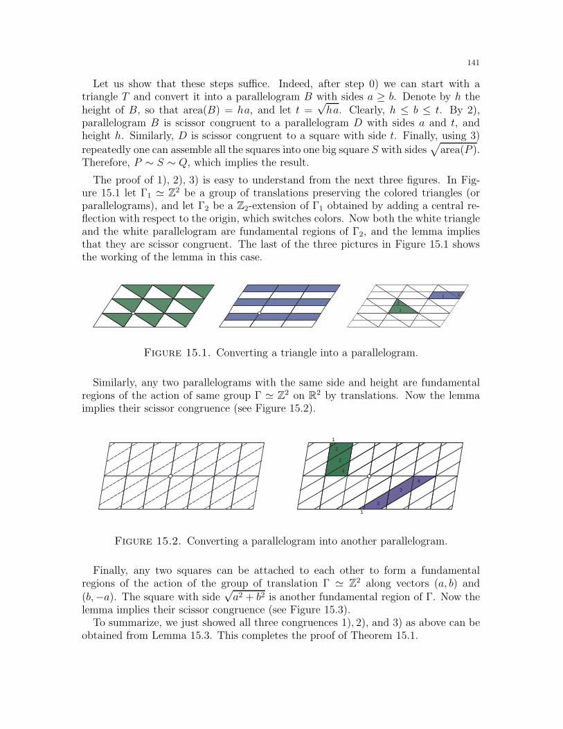
141

Let us show that these steps suffice. Indeed, after step 0) we can start with atriangle T and convert it into a parallelogram B with sides a ≥ b. Denote by h theheight of B, so that area(B) = ha, and let t =

√ha. Clearly, h ≤ b ≤ t. By 2),

parallelogram B is scissor congruent to a parallelogram D with sides a and t, andheight h. Similarly, D is scissor congruent to a square with side t. Finally, using 3)

repeatedly one can assemble all the squares into one big square S with sides√

area(P ).Therefore, P ∼ S ∼ Q, which implies the result.

The proof of 1), 2), 3) is easy to understand from the next three figures. In Fig-ure 15.1 let Γ1 ≃ Z2 be a group of translations preserving the colored triangles (orparallelograms), and let Γ2 be a Z2-extension of Γ1 obtained by adding a central re-flection with respect to the origin, which switches colors. Now both the white triangleand the white parallelogram are fundamental regions of Γ2, and the lemma impliesthat they are scissor congruent. The last of the three pictures in Figure 15.1 showsthe working of the lemma in this case.

1

1

2

2

Figure 15.1. Converting a triangle into a parallelogram.

Similarly, any two parallelograms with the same side and height are fundamentalregions of the action of same group Γ ≃ Z2 on R2 by translations. Now the lemmaimplies their scissor congruence (see Figure 15.2).

1

1

2

2

3

3

4

4

Figure 15.2. Converting a parallelogram into another parallelogram.

Finally, any two squares can be attached to each other to form a fundamentalregions of the action of the group of translation Γ ≃ Z2 along vectors (a, b) and(b,−a). The square with side

√a2 + b2 is another fundamental region of Γ. Now the

lemma implies their scissor congruence (see Figure 15.3).To summarize, we just showed all three congruences 1), 2), and 3) as above can be

obtained from Lemma 15.3. This completes the proof of Theorem 15.1.

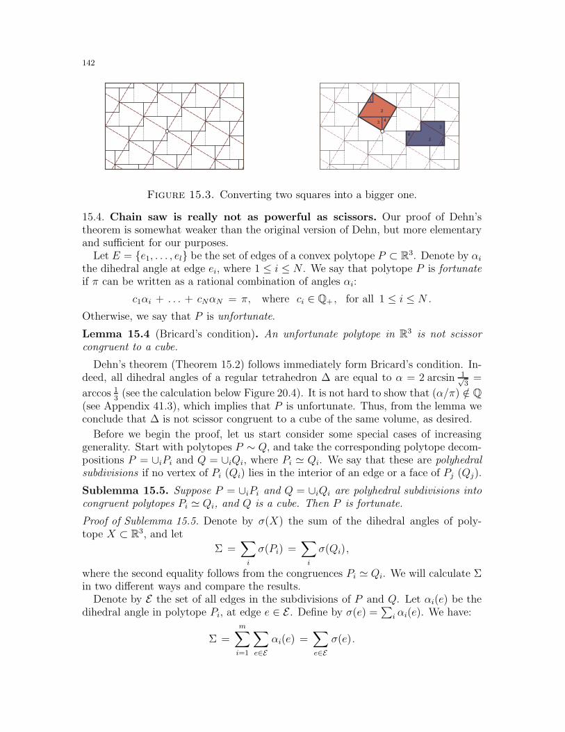
142

1

1

2

3

3

4

4

2

Figure 15.3. Converting two squares into a bigger one.

15.4. Chain saw is really not as powerful as scissors. Our proof of Dehn’stheorem is somewhat weaker than the original version of Dehn, but more elementaryand sufficient for our purposes.

Let E = e1, . . . , el be the set of edges of a convex polytope P ⊂ R3. Denote by αithe dihedral angle at edge ei, where 1 ≤ i ≤ N . We say that polytope P is fortunateif π can be written as a rational combination of angles αi:

c1αi + . . . + cNαN = π, where ci ∈ Q+ , for all 1 ≤ i ≤ N .

Otherwise, we say that P is unfortunate.

Lemma 15.4 (Bricard’s condition). An unfortunate polytope in R3 is not scissorcongruent to a cube.

Dehn’s theorem (Theorem 15.2) follows immediately form Bricard’s condition. In-deed, all dihedral angles of a regular tetrahedron ∆ are equal to α = 2 arcsin 1√

3=

arccos 13

(see the calculation below Figure 20.4). It is not hard to show that (α/π) /∈ Q(see Appendix 41.3), which implies that P is unfortunate. Thus, from the lemma weconclude that ∆ is not scissor congruent to a cube of the same volume, as desired.

Before we begin the proof, let us start consider some special cases of increasinggenerality. Start with polytopes P ∼ Q, and take the corresponding polytope decom-positions P = ∪iPi and Q = ∪iQi, where Pi ≃ Qi. We say that these are polyhedralsubdivisions if no vertex of Pi (Qi) lies in the interior of an edge or a face of Pj (Qj).

Sublemma 15.5. Suppose P = ∪iPi and Q = ∪iQi are polyhedral subdivisions intocongruent polytopes Pi ≃ Qi, and Q is a cube. Then P is fortunate.

Proof of Sublemma 15.5. Denote by σ(X) the sum of the dihedral angles of poly-tope X ⊂ R3, and let

Σ =∑

i

σ(Pi) =∑

i

σ(Qi),

where the second equality follows from the congruences Pi ≃ Qi. We will calculate Σin two different ways and compare the results.

Denote by E the set of all edges in the subdivisions of P and Q. Let αi(e) be thedihedral angle in polytope Pi, at edge e ∈ E . Define by σ(e) =

∑i αi(e). We have:

Σ =

m∑

i=1

∑

e∈Eαi(e) =

∑

e∈Eσ(e).

143

Now observe that σ(e) = 2π when e is an interior edge, σ(e) = π when e is on theboundary of P , and σ(e) = αs when e ⊂ es is the (usual) edge of P . We conclude:

Σ =N∑

s=1

ksαs + nπ, for some k1, . . . , kN ∈ N, and n ∈ Z+ .

By the same argument for the decomposition of Q, since all dihedral angles are equalto π/2 in this case, we obtain that Σ = lπ/2 for some l ∈ N. This implies that P isfortunate, as desired.

In the general case, suppose we have vertices which subdivide the edges of Pi intointervals. By analogy with the previous case, denote these intervals by e, and theset of intervals by E . Let ℓe = |e| denote the lengths of the intervals. Similarly, forthe decomposition of Q, denote by E ′ the resulting set of intervals e′, and by ℓe′ theirlengths.

Sublemma 15.6. Let P = ∪iPi and Q = ∪iQi are polytope decompositions intocongruent polytopes Pi ≃ Qi, and Q is a cube. Suppose the lengths of all intervals arerational: ℓe, ℓe′ ∈ Q for all e ∈ E , e′ ∈ E ′. Then P is fortunate.

Proof of Sublemma 15.6. Taking the previous proof as guidance, we now modify thedefinition of Σ to be as follows:

Σ =m∑

i=1

∑

e∈Eℓe αi(e), Σ′ =

m∑

i=1

∑

e′∈E ′

ℓe′ αi(e′),

where αi(e) is the dihedral angle in polytope Pi at interval e ∈ E , and αi(e′) is the

dihedral angle in polytope Qi at interval e′ ∈ E ′.Let us first show that Σ = Σ′. For a polytope X with the set of edges U = E(X),

let σ(X) =∑

u∈U ℓu · α(u) be the sum of the dihedral angles in X weighted by thelength ℓu of the edges u. We have

Σ =

m∑

i=1

∑

u∈E(Pi)

∑

e∈E , e⊂uℓe αi(e) =

m∑

i=1

∑

u∈E(Pi)

ℓu αi(u) =

m∑

i=1

σ(Pi) ,

where the second equality follows by additivity of the interval length along the edge,and because the dihedral angles are equal along the same edge. We conclude:

Σ =

m∑

i=1

σ(Pi) =

m∑

i=1

σ(Qi) = Σ′ ,

as desired. By analogy with the proof above, we can redefine σ(e) =∑

i ℓeαi(e). Wecan then rewrite Σ as

Σ =∑

e∈Eσ(e).

Since all lengths ℓe are rational, by the same argument as above we conclude that

Σ =N∑

s=1

csαs + rπ, for some c1, . . . , cN , r ∈ Q+ .

144

The same argument for the cube Q gives Σ′/π ∈ Q, as desired.

Proof of Lemma 15.4. In full generality, suppose now the interval lengths ℓe are notnecessarily rational. We now change the definition of Σ once again, substitutingvalues of a general function f : E → R and g : E ′ → R in place of the interval lengths:

Σf =m∑

i=1

∑

e⊂Ef(e)αi(e) , Σ′

g =m∑

i=1

∑

e′⊂E ′

g(e) βi(e′) .

If we can find positive functions f, g as above so that f(e), g(e′) ∈ Q+ for all e ∈ Eand e′ ∈ E ′, and such that Σ = Σ′, the result of the lemma then follows by the sameargument as in the proof above.34

Let us write the conditions the functions f, g need to satisfy to guarantee Σf = Σ′g.

Again, by the argument in the proof above, it suffices to check that the sum alongthe edge u ∈ E(Pi) is equal to that along the corresponding edge u′ ∈ E(Qi):

(ℑ)∑

e∈E , e⊂uf(e) =

∑

e′∈E ′ , e′⊂u′g(e′)

Think of (ℑ) as a set of linear equations for the values f(e), g(e′) which must holdfor all polytopes Pi and all edges u ∈ E(Pi). Because ℓe is an obvious positive realsolution of (ℑ), there is also a positive rational solution of (ℑ). From above, thisfinishes the proof of the lemma.

15.5. Exercises.

Exercise 15.1. (Method of exhaustion) ♦ [1-] Let P,Q ⊂ R3 be two convex polytopessuch that vol(P ) < vol(Q). Prove that there exists a polytope P ′ ⊂ Q, such that P ∼ P ′.

Exercise 15.2. (Extended Bricard’s condition) ♦ [1-] Let P,Q ⊂ R3 be scissor congruentconvex polytopes. Denote by α1, . . . , αm and β1, . . . , βn their dihedral angles. Prove that

r1α1 + . . . + rmαm = s1β1 + . . . + snβn + kπ ,

for some ri, sj ∈ N and k ∈ Z.

Exercise 15.3. (Mirror symmetry) ♦ [1] Let P,P ′ ⊂ R3 be two polyhedra which arecongruent up to a mirror symmetry. Prove that P ∼ P ′.

Exercise 15.4. (Parallelepipeds) ♦ a) [1] Let R be a parallelepiped in R3. Prove that Ris rectifiable (i.e., scissor congruent to a cube of equal volume).b) [1-] Prove that the union of two rectifiable polytopes is also rectifiable.c) [1] Extends parts a) and b) to higher dimensions.

Exercise 15.5. (Prisms) ♦ Define a prism in R3 to be the Minkowski sum of a convexpolygon in a plane and a line segment.a) [1-] Prove that every prism is rectifiable (scissor congruent to a cube of equal volume).b) [1] Prove that polytopes Bi in the proof of Lemma 16.6 can be decomposed into twoprisms. This gives an alternative proof that Bi is rectifiable.

34We need positivity to ensure that all coefficients ci > 0 in the definition of a fortunate polytope.

145

Exercise 15.6. (Zonotopes) [1-] By Exercise 7.16, recall that every zonotope can be sub-divided into parallelepipeds. Use Exercise 15.4 to conclude that every zonotope is scissorcongruent to a cube.

Exercise 15.7. (Hadwiger–Glur) Two polytopes P,Q ⊂ Rd are called T -congruent ifthey are unions of a finite number of simplices which are equal up to translations. They arecalled S-congruent if central symmetries are also allowed.a) [1] Prove the following extension of Theorem 15.1: every two polygons P,Q ⊂ R2 of thesame area are S-equivalent.b) [1+] Prove that a convex polygon Q ⊂ R2 is T -congruent to a square of equal area if andonly if Q is centrally symmetric.c) [1+] Prove that every parallelepiped in R3 is T -congruent to a cube of equal volume.d) [2-] Prove that a convex polytope P ⊂ R3 is T -congruent to a cube of equal volume isand only if P is a zonotope.

Exercise 15.8. Two polytopes P,Q ⊂ Rd are called D-congruent if P can be decomposedinto smaller polytopes which can then rearranged to Q, such that the boundary pointsremain on the boundary. Think of the boundary ∂P as painted, so the goal is to keep thepaint outside (see Figure 15.4).35

Figure 15.4. Two examples of D-congruent polygons.

a) [1] In the plane, prove that every two polygons with the same area and perimeter areD-congruent.b) [1+] In R3, prove that two scissor congruent polytopes with the same volume and surfacearea are D-congruent.c) [1-] In R4, find two scissor congruent polytopes with the same volume and surface area,which are not D-congruent.

Exercise 15.9. Two unbounded convex polyhedra are called scissor congruent if one canbe decomposed to a finite number of (bounded or unbounded) convex polyhedra which canbe assembled into the other.a) [1-] Prove that this is an equivalence relation.b) [1-] In the plane, show that infinite cones with different angles are not scissor congruent.c) [1+] In the plane, let C ⊂ C ′ be two unbounded convex polygons such that C ′ r C isbounded. Prove that C and C ′ are scissor congruent.d) [∗] Prove or disprove the 3-dimensional analogue of part c).

Exercise 15.10. (Tiling with crosses) [1] A cross in Rd is a union of 2d + 1 unit cubes,where one cube in the center is attached to others by a facet. Prove that crosses can tilethe whole space Rd.

35Just as in the definition of scissor congruence, the boundary condition requirement only concernsthe (d− 1)-dimensional faces of P ; we ignore the lower dimensional boundary.

146

Exercise 15.11. (Tiling with notched cubes) A notched cube R(a1, . . . , ad) ⊂ Rd, where0 < a1, . . . , ad < 1, is defined as follows:

R(a1, . . . , ad) = (x1, . . . , xd) ∈ Rd | 0 ≤ xi ≤ 1, and xi ≤ ai for some i.a) [1+] Prove that notched cube R(a1, . . . , ad) can tile the whole space Rd, for all ai asabove.b) [2-] Find all such tilings.c) [1] Prove that no notched cube can tile a brick.

Exercise 15.12. (Reptiles) A (non-convex) polytope P ⊂ Rd is called a reptile if it cantile a copy cP of the same tile, for some c > 1. The order of a reptile is the smallest numberN = cd needed for such a tiling.a) [1-] Prove that every triangle is a reptile of order 4.b) [1-] Prove that a trapezoid with sides 2, 1, 1 and 1 is a reptile of order 4. Similarly, provethat a trapezoid with sides 3, 2, 1 and 2 is a reptile of order 9.c) [1] Find all rectangular reptiles of order at most 5.d) [1] Show that notched cube R(1

2 , . . . ,12) is a reptile of order 2d − 1.

e) [1] Suppose polytope P ⊂ Rd is a reptile of order N . Iterate the tiling construction bytiling bigger and bigger regions with more and more copies of P . Show that this constructiondefines a limit tiling of the whole space, called a substitution tiling.f) [1-] For reptiles in parts a) and b), check whether the resulting tiling of the plane isperiodic or aperiodic.36

g) [1] Check that the substitution tiling of Rd with notched cube is periodic (cf. Exer-cise 15.11).

Exercise 15.13. (Knotted tiles) [2] For every knot K ⊂ R3, prove that there exists a(non-convex) polytope isotopic to K, which can tile the whole space R3.

Exercise 15.14. Let Q ⊂ R2 be a convex set of unit area, area(Q) = 1, and let Q1, . . . , Qnbe its translations. Suppose n is odd. Denote by A the set of points covered by an oddnumber of Qi’s.a) [1-] Suppose Q is a square. Prove that area(A) ≥ 1.b) [1-] Same for the regular hexagon.c) [1] Show that convexity is necessary: if Q is non-convex, we can have area(A) < 1.d) [1+] Show that if Q is a regular triangle, we can have area(A) < 1. For n = 3, find thesmallest possible such area.e) [∗] What happens for a regular octagon? What about when Q is a circle? How aboutgeneral centrally symmetric convex sets?

Exercise 15.15. (ϕ-congruence) Let ϕ : Rd → R be a linear function non-constant on theaxis. Two polytopes P,Q ⊂ Rd are called ϕ-congruent if they are unions of a finite numberof simplices which are equal up to ϕ-invariant translations.a) [1] Suppose ϕ(x, y, z) = ax+ by+ cz, is a linear function on R3, where a, b, c ∈ N. Provethat the following two bricks are ϕ-congruent:

B1 = (x, y, z) | 0 ≤ x ≤ b, 0 ≤ y ≤ c, 0 ≤ z ≤ a,B2 = (x, y, z) | 0 ≤ x ≤ c, 0 ≤ y ≤ a, 0 ≤ z ≤ b.

36There is certain degree of ambiguity in the definition of the substitution tiling. Thus, in eachcase, check whether one can obtain an aperiodic tiling.

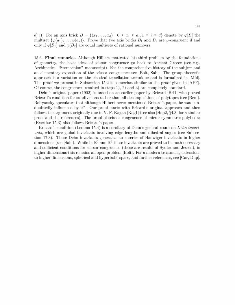
147

b) [1] For an axis brick B = (x1, . . . , xd) | 0 ≤ xi ≤ ai, 1 ≤ i ≤ d denote by ϕ[B] themultiset ϕ(a1), . . . , ϕ(ad). Prove that two axis bricks B1 and B2 are ϕ-congruent if andonly if ϕ[B1] and ϕ[B2] are equal multisets of rational numbers.

15.6. Final remarks. Although Hilbert motivated his third problem by the foundationsof geometry, the basic ideas of scissor congruence go back to Ancient Greece (see e.g.,Archimedes’ “Stomachion” manuscript). For the comprehensive history of the subject andan elementary exposition of the scissor congruence see [Bolt, Sah]. The group theoreticapproach is a variation on the classical tessellation technique and is formalized in [Mul].The proof we present in Subsection 15.2 is somewhat similar to the proof given in [AFF].Of course, the congruences resulted in steps 1), 2) and 3) are completely standard.

Dehn’s original paper (1902) is based on an earlier paper by Bricard [Bri1] who provedBricard’s condition for subdivisions rather than all decompositions of polytopes (see [Ben]).Boltyansky speculates that although Hilbert never mentioned Bricard’s paper, he was “un-doubtedly influenced by it”. Our proof starts with Bricard’s original approach and thenfollows the argument originally due to V. F. Kagan [Kag1] (see also [Hop2, §4.3] for a similarproof and the references). The proof of scissor congruence of mirror symmetric polyhedra(Exercise 15.3) also follows Bricard’s paper.

Bricard’s condition (Lemma 15.4) is a corollary of Dehn’s general result on Dehn invari-ants, which are global invariants involving edge lengths and dihedral angles (see Subsec-tion 17.3). These Dehn invariants generalize to a series of Hadwiger invariants in higherdimensions (see [Sah]). While in R3 and R4 these invariants are proved to be both necessaryand sufficient conditions for scissor congruence (these are results of Sydler and Jessen), inhigher dimensions this remains an open problem [Bolt]. For a modern treatment, extensionsto higher dimensions, spherical and hyperbolic space, and further references, see [Car, Dup].

148

16. Polytope algebra

This is the second of the three sections on scissor congruence. Here we developan algebraic approach, by introducing certain algebraic operations on the polytopeswhich preserve scissor congruence. This approach allows us to prove that certainfamilies of polytopes are scissor congruent, while others are not, all without actuallyexhibiting the decompositions or computing the dihedral angles. Curiously, the al-gebraic approach is almost completely independent of the previous section. In thissection we do not fully develop the theory; instead, we present only the most basictools and concentrate on attractive examples. Among other things, we prove that allpolytopes which tile the space periodically are scissor congruent to a cube, a resultof particular interest, related to classical problems on tilings.

16.1. The power of negative thinking. While the Bricard condition in Lemma 15.4(see also a straightforward extension in Exercise 15.2) resolves Hilbert’s original prob-lem by giving necessary conditions for the scissor congruence, it is very restrictive anddoes not give a sufficient condition. Nor is it easy to use, as one is asked to computethe dihedral angles and verify their rational independence. In fact, even the statementof Bricard’s condition is somewhat misleading, as it suggests that scissor congruenceis a property of dihedral angles.37 The following result is an easy corollary of themain results in this section, and gives a flavor of things to come.

Theorem 16.1 (Sydler). A regular tetrahedron is not scissor congruent to a disjointunion of k ≥ 2 regular tetrahedra, not necessarily of the same size.

Let us emphasize that the dihedral angles are all equal in this case, so one needsto find other tools to prove this result. Let us note that Dehn’s theorem combinedwith the above Sydler’s theorem implies that the cube, the regular tetrahedron andthe regular triangular bipyramid (see Figure 19.1) of the same volume are not scissorcongruent. In other words, there are at least three equivalence classes of polytopesof the same volume. In Exercise 16.1 we will show that there is a continuum of suchequivalence classes.

We first develop and prove several technical algebraic tools and only then returnto further examples and applications.

16.2. Rectifiable polytopes and operations on polytopes. We say that a poly-tope P ⊂ R3 is rectifiable if it is scissor congruent to a cube of equal volume. Forexample, all parallelepipeds are rectifiable by Exercise 15.4. Denote by P ⊕ Q thedisjoint union of polytopes P,Q ⊂ R3. One can show that the disjoint union of rec-tifiable polytopes is also rectifiable (see Exercise 15.4). Let n!×!P = P ⊕ . . .⊕ P (ntimes) denotes the disjoint union of n copies of P .

Polytopes cP obtained by an expansion of P by a factor c > 0, are called similarto P . Obviously, polytopes similar to a rectifiable polytope are also rectifiable. Denoteby R the set of rectifiable polytopes.

37The proof of Bricard’s condition given in the previous section is somewhat more revealing, asit is crucially based on the edge lengths.

149

We say that a polytope P ⊂ R3 is self-similar if it is scissor congruent to a disjointunion of two or more polytopes similar to P . For the rest of this section we use ⊕ todenote the disjoint union of polytopes, and write this as

P ∼ c1P ⊕ . . . ⊕ ckP , where ci > 0, k ≥ 2.

The main result of this section is the following theorem.

Theorem 16.2 (Sydler’s criteria). A polytope P ⊂ R3 is rectifiable if and only if Pis self-similar. Alternatively, P is rectifiable if and only if P ∼ cP ⊕ R, for someR ∈ R and c < 1.

Sydler’s theorem (Theorem 16.1) follows immediately from here. Indeed, if a regulartetrahedron is self-similar, then by the above theorem it must be rectifiable, whichcontradicts Dehn’s theorem (Theorem 15.2).

Before we move to the proof of Sydler’s criteria, let us present two other usefulproperties of scissor congruence. They can be viewed as saying that rectifiability ofpolytopes is invariant under “subtraction” and “division”. As we show later in thissection, these properties allow a remarkable degree of flexibility in deciding whethera given polytope is rectifiable.

Theorem 16.3 (Complementarity lemma). Suppose polytopes A,B,C,D ⊂ R3 sat-isfy: A⊕ B ∼ C ⊕D and B ∼ D. Then A ∼ C.

In particular, the complement of a rectifiable polytope inside a brick is also recti-fiable.

Theorem 16.4 (Tiling lemma). Let P ⊂ R3 be a polytope such that P1⊕ . . .⊕Pm isrectifiable, where every Pi is either congruent to P or a mirror image of P , 1 ≤ i ≤ m.Then P is also rectifiable.

In other words, if we can tile a parallelepiped with copies of a given polytope, thenthis polytope is rectifiable. We say that a tiling of the space R3 is periodic if thereexist three independent vectors such that the tiling is invariant under translations bythese vectors. Obviously, if a polytope tiles a parallelepiped, it has a periodic tilingof the space.

Corollary 16.5. Let P ⊂ R3 be a polytope which tiles the space periodically. Then Pis rectifiable.

Proof. Fix a periodic tiling of R3 by P and let Q be a fundamental parallelepiped ofthe translation group which preserves the tiling. By Lemma 15.3, parallelepiped Qis scissor congruent to a disjoint union of copies of P and mirror symmetric copiesof P . Since Q ∈ R, by the tiling lemma (Theorem 16.4) so is P .

16.3. Proofs of the theorems. We start with an important technical result.

Lemma 16.6. Let P ⊂ R3 be a polytope and let α1, . . . , αk > 0 be fixed positive realnumbers, such that α1 + . . .+ αk = 1. Then

P ∼ α1P ⊕ . . . ⊕ αkP ⊕ R,

150

for some R ∈ R.

Proof. First, let us show that it suffices to prove the result for the tetrahedra. Indeed,suppose P = ∪mi=1∆i and

∆i ∼ α1∆i ⊕ . . . ⊕ αk∆i ⊕ Ri for all 1 ≤ i ≤ m.

Then

P ∼k⊕

j=1

[m⊕

i=1

αj∆i

]⊕[

m⊕

i=1

Ri

]∼ α1P ⊕ . . . ⊕ αkP ⊕ R,

where we are using the fact R1 ⊕ . . .⊕ Rm ∈ R (see Exercise 15.4).Let us prove the result in a special case. Let ∆ ⊂ R3 be a standard tetrahedron

defined by the equations x, y, z ≥ 0 and x+y+z ≤ 1. Cut the tetrahedron into layers0 ≤ z ≤ α1, α1 ≤ z ≤ α1 + α2, etc. Remove the tetrahedra αi∆i, 1 ≤ i ≤ k, fromthe corners of the corresponding layers, as shown in Figure 16.1. Denote by Bi theremaining hexahedron (polytope with 6 faces) in the i-th layer, for all 1 ≤ i ≤ k − 1(the k-th layer is equal to αk∆). Observe that each Bi is scissor congruent to a brick(see Figure 16.1). By Exercise 15.4, this implies that B1⊕B2⊕. . .⊕Bk−1 is rectifiable,and finishes the proof.

∆Qi

Bi

B1

B2

B3

α1∆

α2∆

α3∆

α4∆

Figure 16.1. Layers Bi ∪ αi∆ and scissor congruence Bi ∼ Qi.

For the general tetrahedra, use a construction obtained via a linear transformation.The image of a brick is a parallelepiped which are rectifiable by Exercise 15.4.

Proof of Theorem 16.4. Since the mirror image of polytope P is scissor congruent to P(see Exercise 15.3), it suffices to prove the result for congruent polytopes Pi ∼ P . Thetheorem and Lemma 16.6 can be written as:

n×P ∼ R1 , nP ∼ (n×P ) ⊕ R2 ,

for some R1, R2 ∈ R. We conclude:

nP ∼ (n×P ) ⊕ R2 ∼ R1 ⊕ R2 ∈ R,as desired.

Proof of Theorem 16.3. First, observe that

vol(A) = vol(A⊕ B) − vol(A) = vol(C ⊕D) − vol(D) = vol(C).

151

Fix a large enough integer n and define

A′ =1

nA, B′ =

1

nB, C ′ =

1

nC, D′ =

1

nD.

By Lemma 16.6, we have:

A ∼ (n×A′) ⊕ R1, C ∼ (n×C ′) ⊕R2 ,

for some R1, R2 ∈ R. From above,

vol(R1) =(1− n

n3

)vol(A) =

(1− n

n3

)vol(C) = vol(R2).

This implies that R1 ∼ R2 and that vol(R1) = (1− 1/n2)vol(A)→ vol(A) as n→∞.Therefore, vol(n × B′)/vol(A) → 0 as n → ∞, and for sufficiently large n we canarrange n copies of B′ inside R1.

38 In other words, for large enough n, we have

R ∼ (n×B′) ⊕ S,

for some polytope S ⊂ R3. We then have:

A ∼ (n×A′) ⊕ R1 ∼ (n×A′) ⊕ (n×B′) ⊕ S ∼ n×(A′ ⊕B′) ⊕ S

∼ n×(C ′ ⊕D′) ⊕ S ∼ (n×C ′) ⊕ (n×D′) ⊕ S

∼ (n×C ′) ⊕ (n×B′) ⊕ S ∼ (n×C ′) ⊕ R1 ∼ (n×C ′) ⊕ R2 ∼ C,

as desired.

Proof of Theorem 16.2. The “only if” part is trivial in both parts. For the secondcriterion, by Lemma 16.6, we have:

cP ⊕ R ∼ P ∼ cP ⊕ (1− c)P ⊕ R′,

for some R,R′ ∈ R. By the complementarity lemma (Theorem 16.3), we get (1 −c)P ⊕R′ ∼ R. Write R ∼ R′⊕R′′ for some R′′ ∈ R. After another application of thecomplementarity lemma, we obtain (1− c)P ∈ R, as desired.

For the first part, P ∼ c1P ⊕ . . .⊕ ckP and let c = c1 + . . .+ ck. By Lemma 16.6,we have:

cP ∼ c1P ⊕ . . . ⊕ ckP ⊕ R ∼ P ⊕ R,

for some R ∈ R. Now the second criterion we just proved implies that P ∈ R.

16.4. Examples and special cases. Let O = (0, 0, 0), a = (1, 0, 0), b = (0, 1, 0), c =(0, 0, 1), and d = (1, 1, 0). Consider the standard tetrahedron ∆1 = convO, a, b, cand the Hill tetrahedron ∆2 = convO, b, c, d. Clearly, vol(∆1) = vol(∆2) = 1/6.

Proposition 16.7. The standard tetrahedron, Hill tetrahedron and the regular tetra-hedron of equal volume are not scissor congruent.

38Formally speaking, this still requires an argument (see Exercise 15.1).

152

Proof. First, let us show that ∆2 is rectifiable. To see this, observe that six copiesof ∆2 tile the unit cube C = [0, 1]3. Indeed, take each copy to be a convex hull of apath from O to (1, 1, 1) as shown in Figure 16.2 (there are six such paths), and usethe tiling lemma. By Dehn’s theorem (Theorem 15.2), this implies that ∆0 ≁ ∆2,where ∆0 is the regular tetrahedron of volume 1/6.

∆1∆2 c∆0

Figure 16.2. Hill tetrahedron, standard tetrahedron and the regular tetrahedron.

To see that ∆1 is not rectifiable, remove four copies of ∆1 from the cube C asshown in Figure 16.2. We are left with a regular tetrahedron c∆0, c = 3

√2, which by

Dehn’s theorem is not rectifiable. By the complementarity lemma, we conclude thatthe above union of four copies of ∆1 is not rectifiable, and by the tiling lemma sois ∆1. This implies that ∆1 ≁ ∆2.

Finally, the same construction shows that ∆0 ≁ ∆1. Otherwise, four copies of ∆0

and one copy of c∆1 are scissor congruent to a cube, which contradicts the firstSydler’s criterion (Theorem 16.2). This completes the proof of Proposition 16.7.

By analogy with the case of a regular tetrahedron, one can use Lemma 15.4 toprove directly that the regular octahedron is not rectifiable. In fact, one can even usethe same proof of the irrationality of dihedral angles (see Subsection 41.2). However,if one wants to avoid calculating dihedral angles this time, here is a neat geometricround about argument.

Proposition 16.8. The regular octahedron is not scissor congruent to the standard,Hill, or regular tetrahedra of the same volume.

Proof. First, observe that the regular octahedron Q can be tiled with eight copies ofa standard tetrahedron. By the tiling lemma this immediately immediately impliesthat Q is not rectifiable, and by the first Sydler’s criterion this implies that Q is notscissor congruent to a standard tetrahedron. We need a separate argument to showthat Q ≁ c∆0.

Take a regular tetrahedron ∆0 and remove four corner tetrahedra ∆′0 = 1

2∆0. We

are left with a regular octahedron Q (see Figure 16.3). Take a disjoint union of Qwith any two of tetrahedra ∆0’. Now, if Q ∼ c∆0, we have:

∆0 ∼ Q⊕ 4×∆′0 ∼ c∆0 ⊕ 4×∆′

0 .

This again contradicts the first Sydler’s criterion (Theorem 16.2).

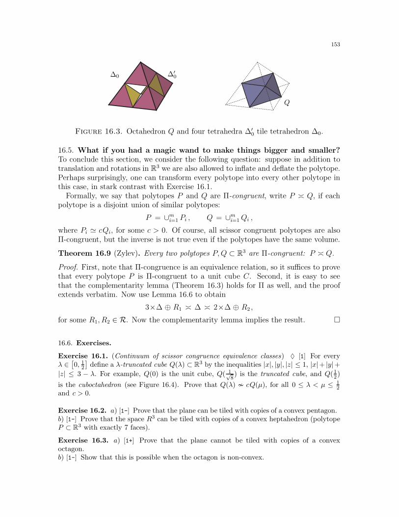
153

∆0 ∆′0

Q

Figure 16.3. Octahedron Q and four tetrahedra ∆′0 tile tetrahedron ∆0.

16.5. What if you had a magic wand to make things bigger and smaller?To conclude this section, we consider the following question: suppose in addition totranslation and rotations in R3 we are also allowed to inflate and deflate the polytope.Perhaps surprisingly, one can transform every polytope into every other polytope inthis case, in stark contrast with Exercise 16.1.

Formally, we say that polytopes P and Q are Π-congruent, write P ≍ Q, if eachpolytope is a disjoint union of similar polytopes:

P = ∪mi=1 Pi , Q = ∪mi=1Qi ,

where Pi ≃ cQi, for some c > 0. Of course, all scissor congruent polytopes are alsoΠ-congruent, but the inverse is not true even if the polytopes have the same volume.

Theorem 16.9 (Zylev). Every two polytopes P,Q ⊂ R3 are Π-congruent: P ≍ Q.

Proof. First, note that Π-congruence is an equivalence relation, so it suffices to provethat every polytope P is Π-congruent to a unit cube C. Second, it is easy to seethat the complementarity lemma (Theorem 16.3) holds for Π as well, and the proofextends verbatim. Now use Lemma 16.6 to obtain

3×∆ ⊕ R1 ≍ ∆ ≍ 2×∆ ⊕ R2 ,

for some R1, R2 ∈ R. Now the complementarity lemma implies the result.

16.6. Exercises.

Exercise 16.1. (Continuum of scissor congruence equivalence classes) ♦ [1] For everyλ ∈

[0, 1

2

]define a λ-truncated cube Q(λ) ⊂ R3 by the inequalities |x|, |y|, |z| ≤ 1, |x|+ |y|+

|z| ≤ 3 − λ. For example, Q(0) is the unit cube, Q( 1√8) is the truncated cube, and Q(1

2)

is the cuboctahedron (see Figure 16.4). Prove that Q(λ) ≁ cQ(µ), for all 0 ≤ λ < µ ≤ 12

and c > 0.

Exercise 16.2. a) [1-] Prove that the plane can be tiled with copies of a convex pentagon.b) [1-] Prove that the space R3 can be tiled with copies of a convex heptahedron (polytopeP ⊂ R3 with exactly 7 faces).

Exercise 16.3. a) [1+] Prove that the plane cannot be tiled with copies of a convexoctagon.b) [1-] Show that this is possible when the octagon is non-convex.

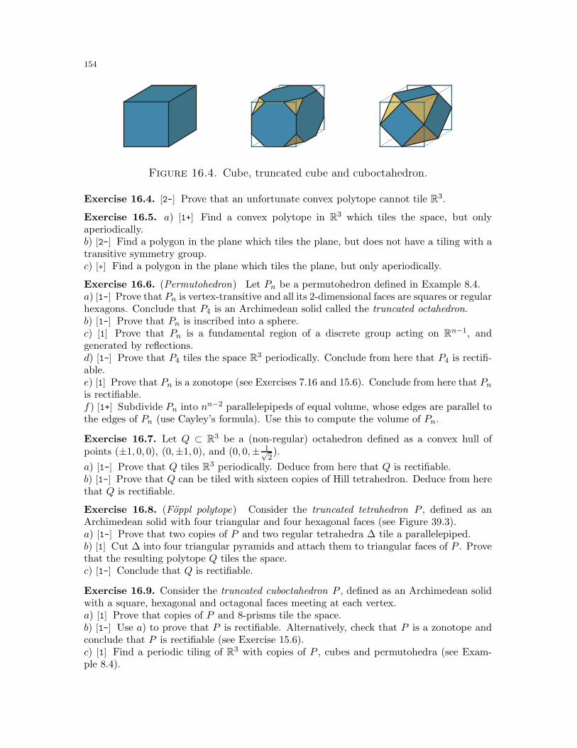
154

Figure 16.4. Cube, truncated cube and cuboctahedron.

Exercise 16.4. [2-] Prove that an unfortunate convex polytope cannot tile R3.

Exercise 16.5. a) [1+] Find a convex polytope in R3 which tiles the space, but onlyaperiodically.b) [2-] Find a polygon in the plane which tiles the plane, but does not have a tiling with atransitive symmetry group.c) [∗] Find a polygon in the plane which tiles the plane, but only aperiodically.

Exercise 16.6. (Permutohedron) Let Pn be a permutohedron defined in Example 8.4.a) [1-] Prove that Pn is vertex-transitive and all its 2-dimensional faces are squares or regularhexagons. Conclude that P4 is an Archimedean solid called the truncated octahedron.b) [1-] Prove that Pn is inscribed into a sphere.c) [1] Prove that Pn is a fundamental region of a discrete group acting on Rn−1, andgenerated by reflections.d) [1-] Prove that P4 tiles the space R3 periodically. Conclude from here that P4 is rectifi-able.e) [1] Prove that Pn is a zonotope (see Exercises 7.16 and 15.6). Conclude from here that Pnis rectifiable.f) [1+] Subdivide Pn into nn−2 parallelepipeds of equal volume, whose edges are parallel tothe edges of Pn (use Cayley’s formula). Use this to compute the volume of Pn.

Exercise 16.7. Let Q ⊂ R3 be a (non-regular) octahedron defined as a convex hull ofpoints (±1, 0, 0), (0,±1, 0), and (0, 0,± 1√

2).

a) [1-] Prove that Q tiles R3 periodically. Deduce from here that Q is rectifiable.b) [1-] Prove that Q can be tiled with sixteen copies of Hill tetrahedron. Deduce from herethat Q is rectifiable.

Exercise 16.8. (Foppl polytope) Consider the truncated tetrahedron P , defined as anArchimedean solid with four triangular and four hexagonal faces (see Figure 39.3).a) [1-] Prove that two copies of P and two regular tetrahedra ∆ tile a parallelepiped.b) [1] Cut ∆ into four triangular pyramids and attach them to triangular faces of P . Provethat the resulting polytope Q tiles the space.c) [1-] Conclude that Q is rectifiable.

Exercise 16.9. Consider the truncated cuboctahedron P , defined as an Archimedean solidwith a square, hexagonal and octagonal faces meeting at each vertex.a) [1] Prove that copies of P and 8-prisms tile the space.b) [1-] Use a) to prove that P is rectifiable. Alternatively, check that P is a zonotope andconclude that P is rectifiable (see Exercise 15.6).c) [1] Find a periodic tiling of R3 with copies of P , cubes and permutohedra (see Exam-ple 8.4).

155

d) [1] Find a periodic tiling of the space with copies of P , truncated cube (see Subsec-tion 16.4) and truncated tetrahedron (see Exercise 16.8).

Exercise 16.10. [1] Give an explicit construction of scissor congruence of the Hill tetra-hedron ∆2 and a prism.

Exercise 16.11. (Rectifiable tetrahedra) Prove that the following tetrahedra (xyzw) ⊂ R3

are rectifiable:a) [1-] x = O, y = (1, 0, 0), z = (1, 1, 1), w = (1,−1, 1);b) [1-] x = O, y = (1,−1,−1), z = (1, 1, 1), w = (1,−1, 1);c) [1-] x = O, y = (2, 0, 0), z = (1, 1, 1), w = (1,−1, 1);d) [1-] x = O, y = (1, 0, 1/2), z = (1, 1, 1), w = (1,−1, 1);e) [1] |xz| = |yw| = 2, |xy| = |xw| = |yz| = |zw| =

√3;

f) [1+] |xy| = |zw| = |yz| = a, |xz| = |yw| = b, |zw| = 3c, where b2 = a2 + 3c2.

Exercise 16.12. (Hill tetrahedra) For every α ∈ (0, 2π/3), let v1, v2, v 3 ∈ R3 be threeunit vectors with angle α between every two of them. Define the Hill tetrahedron Q(α) asfollows:

Q(α) = c1v + c2v 2 + c3v3 | 0 ≤ c1 ≤ c2 ≤ c3 ≤ 1.For example, Q(π/2) is the Hill tetrahedron ∆2 defined earlier.a) [1] Decompose Q(α) into three pieces which assemble into a prism. Conclude that allHill tetrahedra are rectifiable.b) [1+] Find a periodic tiling of space with Q(α). Again, conclude that all Hill tetrahedraare rectifiable.

Exercise 16.13. (Golden tetrahedron) Denote by T ⊂ R3 the golden tetrahedron definedby

x, y, z ≥ 0, φ x + y +z

φ≤ 1, where φ =

1 +√

5

2.

a) [1] Prove that all dihedral angles of T are rational multiples of π. Does T tile the space?b) [1+] Prove that T is rectifiable by an explicit construction.c) [1+] Prove that the Hill tetrahedron Q(2π/5) can be decomposed into four golden tetra-hedra (possibly, of different size).d) [1+] Generalize the tiling lemma (Theorem 16.4) to similar polytopes. Use this andpart c) to give another proof that T is rectifiable.

Exercise 16.14. (Schlafli simplices) For a simplex ∆ = (v1v2 . . . vn+1) ⊂ Rn denoteby Fi the facet containing all vertices except vi. Let G∆ be a graph with the vertices1, 2, . . . , n + 1 and edges (i, j) corresponding to acute dihedral angles between facets Fiand Fj .a) [1+] Prove that G∆ contains a spanning tree. Conclude that ∆ has at least n acutedihedral angles.b) [1] Show that for every spanning tree T in a complete graph Kn+1, there exists a simplex∆ ⊂ Rn with

(n2

)right dihedral angles and n acute dihedral angles corresponding to this

spanning tree: G∆ = T . Such ∆ are called Schlafli simplices.39

c) [1] Show that every Schlafli simplex corresponding to tree T is a convex hull of mutuallyorthogonal intervals which form a tree isomorphic to T .d) [1] Denote by ℓij the length of the edge (vivj), and by ai the length of the altitude in ∆from vertex vi. Prove that cos γij = aiaj/ℓij , where γij is the dihedral angle at (vivj).

39H. S. M. Coxeter calls these simplices orthogonal trees.

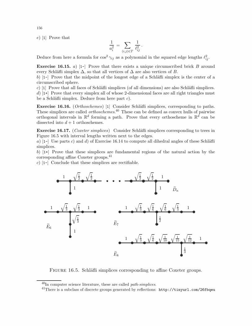
156

e) [1] Prove that1

a2i

=∑

(i,j)∈T

1

ℓ2ij.

Deduce from here a formula for cos2 γij as a polynomial in the squared edge lengths ℓ2ij.

Exercise 16.15. a) [1-] Prove that there exists a unique circumscribed brick B aroundevery Schlafli simplex ∆, so that all vertices of ∆ are also vertices of B.b) [1-] Prove that the midpoint of the longest edge of a Schlafli simplex is the center of acircumscribed sphere.c) [1] Prove that all faces of Schlafli simplices (of all dimensions) are also Schlafli simplices.d) [1+] Prove that every simplex all of whose 2-dimensional faces are all right triangles mustbe a Schlafli simplex. Deduce from here part c).

Exercise 16.16. (Orthoschemes) [1] Consider Schlafli simplices, corresponding to paths.These simplices are called orthoschemes.40 These can be defined as convex hulls of pairwiseorthogonal intervals in Rd forming a path. Prove that every orthoscheme in Rd can bedissected into d+ 1 orthoschemes.

Exercise 16.17. (Coxeter simplices) Consider Schlafli simplices corresponding to trees inFigure 16.5 with interval lengths written next to the edges.a) [1-] Use parts c) and d) of Exercise 16.14 to compute all dihedral angles of these Schlaflisimplices.b) [1+] Prove that these simplices are fundamental regions of the natural action by thecorresponding affine Coxeter groups.41

c) [1-] Conclude that these simplices are rectifiable.

Dn

E6E7

E8

1

11

11

11

1

1

1

1√

12

√12

√12

√12

√13

√13

√13

√13

√13

√13

12

13

√16

√16

√16

√110

√112

√115

Figure 16.5. Schlafli simplices corresponding to affine Coxeter groups.

40In computer science literature, these are called path-simplices.41There is a subclass of discrete groups generated by reflections: http://tinyurl.com/26fbqeu

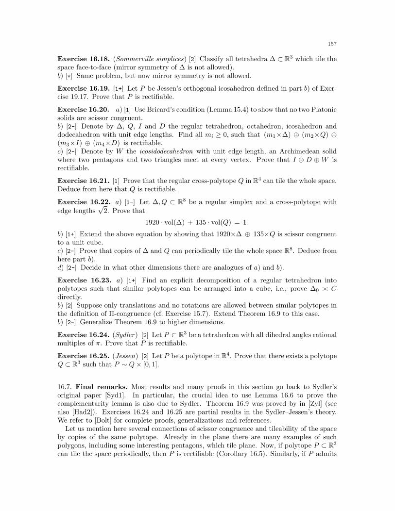
157

Exercise 16.18. (Sommerville simplices) [2] Classify all tetrahedra ∆ ⊂ R3 which tile thespace face-to-face (mirror symmetry of ∆ is not allowed).b) [∗] Same problem, but now mirror symmetry is not allowed.

Exercise 16.19. [1+] Let P be Jessen’s orthogonal icosahedron defined in part b) of Exer-cise 19.17. Prove that P is rectifiable.

Exercise 16.20. a) [1] Use Bricard’s condition (Lemma 15.4) to show that no two Platonicsolids are scissor congruent.b) [2-] Denote by ∆, Q, I and D the regular tetrahedron, octahedron, icosahedron anddodecahedron with unit edge lengths. Find all mi ≥ 0, such that (m1×∆) ⊕ (m2×Q) ⊕(m3×I) ⊕ (m4×D) is rectifiable.c) [2-] Denote by W the icosidodecahedron with unit edge length, an Archimedean solidwhere two pentagons and two triangles meet at every vertex. Prove that I ⊕ D ⊕ W isrectifiable.

Exercise 16.21. [1] Prove that the regular cross-polytope Q in R4 can tile the whole space.Deduce from here that Q is rectifiable.

Exercise 16.22. a) [1-] Let ∆, Q ⊂ R8 be a regular simplex and a cross-polytope with

edge lengths√

2. Prove that

1920 · vol(∆) + 135 · vol(Q) = 1.

b) [1+] Extend the above equation by showing that 1920×∆ ⊕ 135×Q is scissor congruentto a unit cube.c) [2-] Prove that copies of ∆ and Q can periodically tile the whole space R8. Deduce fromhere part b).d) [2-] Decide in what other dimensions there are analogues of a) and b).

Exercise 16.23. a) [1+] Find an explicit decomposition of a regular tetrahedron intopolytopes such that similar polytopes can be arranged into a cube, i.e., prove ∆0 ≍ Cdirectly.b) [2] Suppose only translations and no rotations are allowed between similar polytopes inthe definition of Π-congruence (cf. Exercise 15.7). Extend Theorem 16.9 to this case.b) [2-] Generalize Theorem 16.9 to higher dimensions.

Exercise 16.24. (Sydler) [2] Let P ⊂ R3 be a tetrahedron with all dihedral angles rationalmultiples of π. Prove that P is rectifiable.

Exercise 16.25. (Jessen) [2] Let P be a polytope in R4. Prove that there exists a polytopeQ ⊂ R3 such that P ∼ Q× [0, 1].

16.7. Final remarks. Most results and many proofs in this section go back to Sydler’soriginal paper [Syd1]. In particular, the crucial idea to use Lemma 16.6 to prove thecomplementarity lemma is also due to Sydler. Theorem 16.9 was proved by in [Zyl] (seealso [Had2]). Exercises 16.24 and 16.25 are partial results in the Sydler–Jessen’s theory.We refer to [Bolt] for complete proofs, generalizations and references.

Let us mention here several connections of scissor congruence and tileability of the spaceby copies of the same polytope. Already in the plane there are many examples of suchpolygons, including some interesting pentagons, which tile plane. Now, if polytope P ⊂ R3

can tile the space periodically, then P is rectifiable (Corollary 16.5). Similarly, if P admits

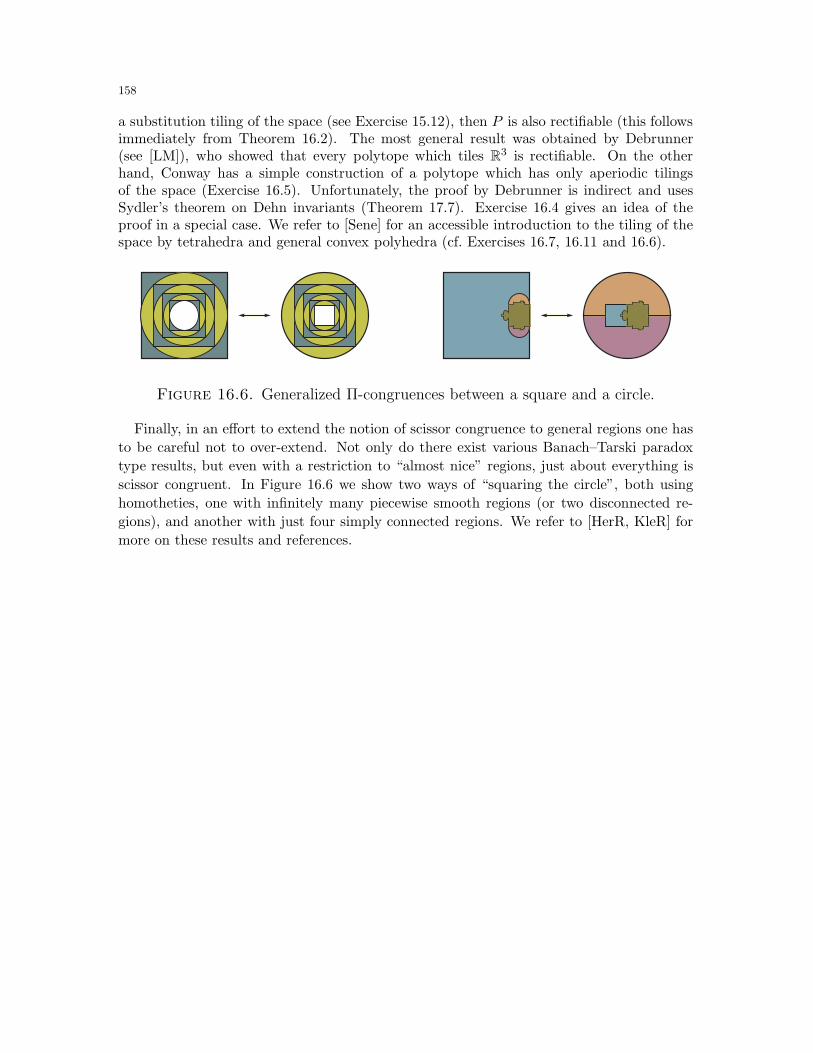
158

a substitution tiling of the space (see Exercise 15.12), then P is also rectifiable (this followsimmediately from Theorem 16.2). The most general result was obtained by Debrunner(see [LM]), who showed that every polytope which tiles R3 is rectifiable. On the otherhand, Conway has a simple construction of a polytope which has only aperiodic tilingsof the space (Exercise 16.5). Unfortunately, the proof by Debrunner is indirect and usesSydler’s theorem on Dehn invariants (Theorem 17.7). Exercise 16.4 gives an idea of theproof in a special case. We refer to [Sene] for an accessible introduction to the tiling of thespace by tetrahedra and general convex polyhedra (cf. Exercises 16.7, 16.11 and 16.6).

Figure 16.6. Generalized Π-congruences between a square and a circle.

Finally, in an effort to extend the notion of scissor congruence to general regions one has

to be careful not to over-extend. Not only do there exist various Banach–Tarski paradox

type results, but even with a restriction to “almost nice” regions, just about everything is

scissor congruent. In Figure 16.6 we show two ways of “squaring the circle”, both using

homotheties, one with infinitely many piecewise smooth regions (or two disconnected re-

gions), and another with just four simply connected regions. We refer to [HerR, KleR] for

more on these results and references.

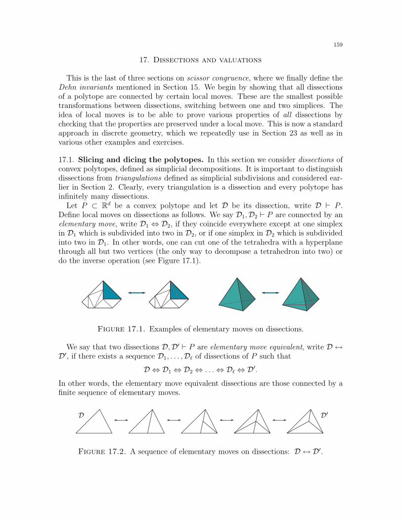
159

17. Dissections and valuations

This is the last of three sections on scissor congruence, where we finally define theDehn invariants mentioned in Section 15. We begin by showing that all dissectionsof a polytope are connected by certain local moves. These are the smallest possibletransformations between dissections, switching between one and two simplices. Theidea of local moves is to be able to prove various properties of all dissections bychecking that the properties are preserved under a local move. This is now a standardapproach in discrete geometry, which we repeatedly use in Section 23 as well as invarious other examples and exercises.

17.1. Slicing and dicing the polytopes. In this section we consider dissections ofconvex polytopes, defined as simplicial decompositions. It is important to distinguishdissections from triangulations defined as simplicial subdivisions and considered ear-lier in Section 2. Clearly, every triangulation is a dissection and every polytope hasinfinitely many dissections.

Let P ⊂ Rd be a convex polytope and let D be its dissection, write D ⊢ P .Define local moves on dissections as follows. We say D1,D2 ⊢ P are connected by anelementary move, write D1 ⇔ D2, if they coincide everywhere except at one simplexin D1 which is subdivided into two in D2, or if one simplex in D2 which is subdividedinto two in D1. In other words, one can cut one of the tetrahedra with a hyperplanethrough all but two vertices (the only way to decompose a tetrahedron into two) ordo the inverse operation (see Figure 17.1).

Figure 17.1. Examples of elementary moves on dissections.

We say that two dissections D,D′ ⊢ P are elementary move equivalent, write D ↔D′, if there exists a sequence D1, . . . ,Dℓ of dissections of P such that

D ⇔ D1 ⇔ D2 ⇔ . . .⇔ Dℓ ⇔ D′.

In other words, the elementary move equivalent dissections are those connected by afinite sequence of elementary moves.

D D′

Figure 17.2. A sequence of elementary moves on dissections: D ↔ D′.

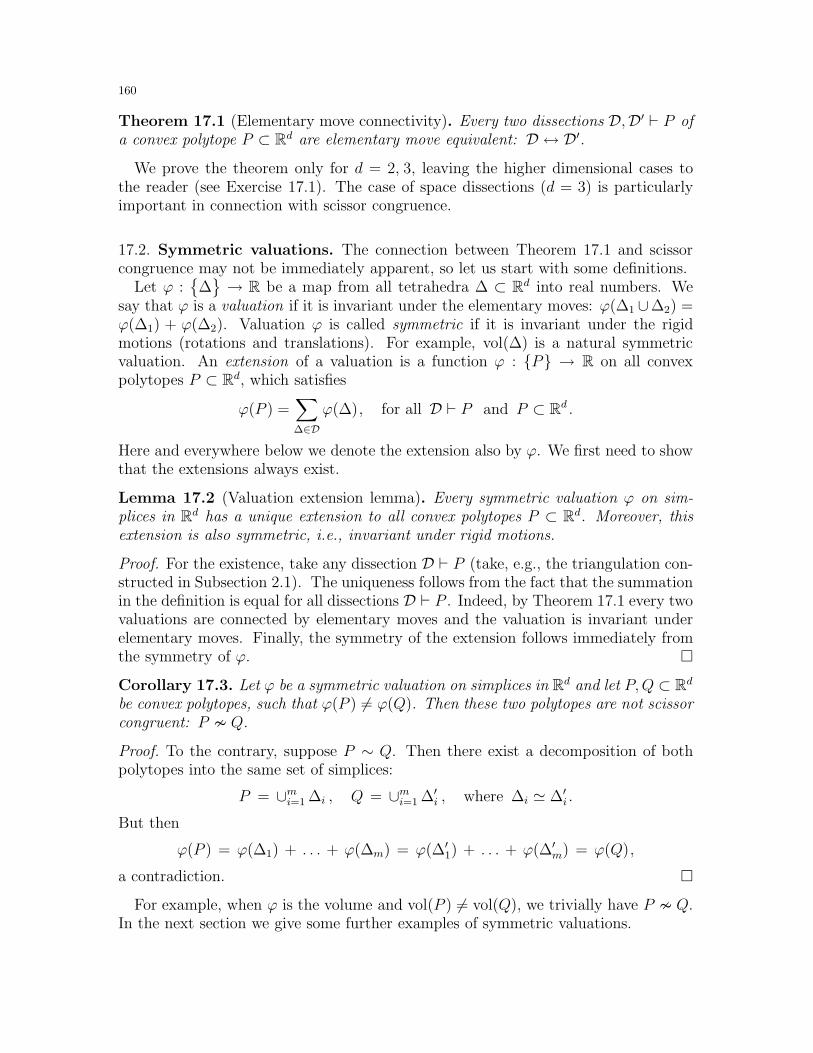
160

Theorem 17.1 (Elementary move connectivity). Every two dissections D,D′ ⊢ P ofa convex polytope P ⊂ Rd are elementary move equivalent: D ↔ D′.

We prove the theorem only for d = 2, 3, leaving the higher dimensional cases tothe reader (see Exercise 17.1). The case of space dissections (d = 3) is particularlyimportant in connection with scissor congruence.

17.2. Symmetric valuations. The connection between Theorem 17.1 and scissorcongruence may not be immediately apparent, so let us start with some definitions.

Let ϕ :∆→ R be a map from all tetrahedra ∆ ⊂ Rd into real numbers. We

say that ϕ is a valuation if it is invariant under the elementary moves: ϕ(∆1 ∪∆2) =ϕ(∆1) + ϕ(∆2). Valuation ϕ is called symmetric if it is invariant under the rigidmotions (rotations and translations). For example, vol(∆) is a natural symmetricvaluation. An extension of a valuation is a function ϕ : P → R on all convexpolytopes P ⊂ Rd, which satisfies

ϕ(P ) =∑

∆∈Dϕ(∆), for all D ⊢ P and P ⊂ Rd .

Here and everywhere below we denote the extension also by ϕ. We first need to showthat the extensions always exist.

Lemma 17.2 (Valuation extension lemma). Every symmetric valuation ϕ on sim-plices in Rd has a unique extension to all convex polytopes P ⊂ Rd. Moreover, thisextension is also symmetric, i.e., invariant under rigid motions.

Proof. For the existence, take any dissection D ⊢ P (take, e.g., the triangulation con-structed in Subsection 2.1). The uniqueness follows from the fact that the summationin the definition is equal for all dissections D ⊢ P . Indeed, by Theorem 17.1 every twovaluations are connected by elementary moves and the valuation is invariant underelementary moves. Finally, the symmetry of the extension follows immediately fromthe symmetry of ϕ.

Corollary 17.3. Let ϕ be a symmetric valuation on simplices in Rd and let P,Q ⊂ Rdbe convex polytopes, such that ϕ(P ) 6= ϕ(Q). Then these two polytopes are not scissorcongruent: P ≁ Q.

Proof. To the contrary, suppose P ∼ Q. Then there exist a decomposition of bothpolytopes into the same set of simplices:

P = ∪mi=1 ∆i , Q = ∪mi=1 ∆′i , where ∆i ≃ ∆′

i .

But then

ϕ(P ) = ϕ(∆1) + . . . + ϕ(∆m) = ϕ(∆′1) + . . . + ϕ(∆′

m) = ϕ(Q),

a contradiction.

For example, when ϕ is the volume and vol(P ) 6= vol(Q), we trivially have P ≁ Q.In the next section we give some further examples of symmetric valuations.

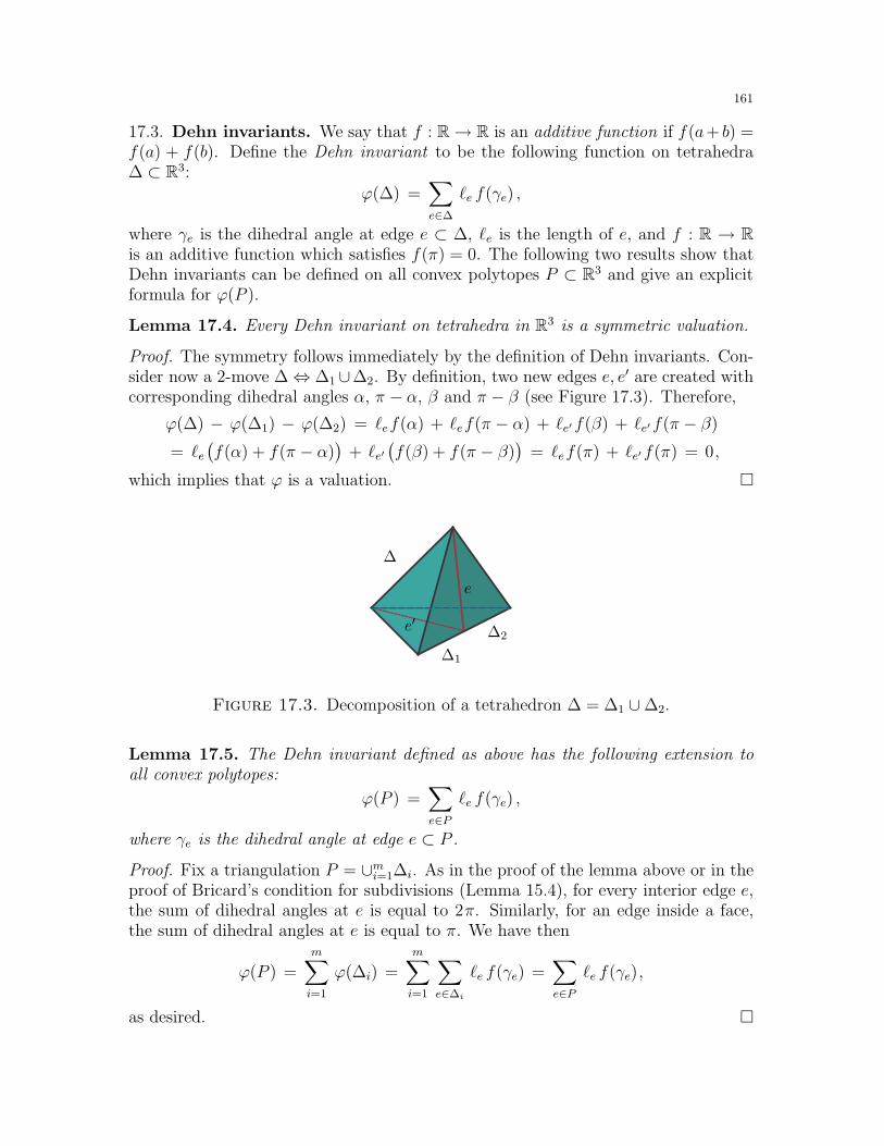
161

17.3. Dehn invariants. We say that f : R→ R is an additive function if f(a+ b) =f(a) + f(b). Define the Dehn invariant to be the following function on tetrahedra∆ ⊂ R3:

ϕ(∆) =∑

e∈∆

ℓe f(γe) ,

where γe is the dihedral angle at edge e ⊂ ∆, ℓe is the length of e, and f : R → Ris an additive function which satisfies f(π) = 0. The following two results show thatDehn invariants can be defined on all convex polytopes P ⊂ R3 and give an explicitformula for ϕ(P ).

Lemma 17.4. Every Dehn invariant on tetrahedra in R3 is a symmetric valuation.

Proof. The symmetry follows immediately by the definition of Dehn invariants. Con-sider now a 2-move ∆⇔ ∆1∪∆2. By definition, two new edges e, e′ are created withcorresponding dihedral angles α, π − α, β and π − β (see Figure 17.3). Therefore,

ϕ(∆) − ϕ(∆1) − ϕ(∆2) = ℓef(α) + ℓef(π − α) + ℓe′ f(β) + ℓe′ f(π − β)

= ℓe(f(α) + f(π − α)

)+ ℓe′

(f(β) + f(π − β)

)= ℓef(π) + ℓe′ f(π) = 0,

which implies that ϕ is a valuation.

e

e′

∆

∆1

∆2

Figure 17.3. Decomposition of a tetrahedron ∆ = ∆1 ∪∆2.

Lemma 17.5. The Dehn invariant defined as above has the following extension toall convex polytopes:

ϕ(P ) =∑

e∈Pℓe f(γe) ,

where γe is the dihedral angle at edge e ⊂ P .

Proof. Fix a triangulation P = ∪mi=1∆i. As in the proof of the lemma above or in theproof of Bricard’s condition for subdivisions (Lemma 15.4), for every interior edge e,the sum of dihedral angles at e is equal to 2π. Similarly, for an edge inside a face,the sum of dihedral angles at e is equal to π. We have then

ϕ(P ) =

m∑

i=1

ϕ(∆i) =

m∑

i=1

∑

e∈∆i

ℓe f(γe) =∑

e∈Pℓe f(γe),

as desired.

162

We can now summarize the results as follows.

Theorem 17.6 (Dehn). Define the Dehn invariant on all convex polytopes P ⊂ R3

by the following formula:

ϕ(P ) =∑

e∈Pℓe f(γe) ,

where γe is the dihedral angle at edge e ∈ P , ℓe is the length of e, and where f : R→ Ris an additive function such that f(π) = 0. Suppose now P,Q ⊂ R3 are two convexpolytopes such that ϕ(P ) 6= ϕ(Q). Then P and Q are not scissor congruent: P ≁ Q.

17.4. From abstraction to applications. The Dehn invariants defined above maynot seem like much. In fact, at first glance it might seem too abstract to be useful inactual applications. Before giving several examples, let us state the key result in thefield.

Theorem 17.7 (Sydler). Every two convex polytopes P,Q ⊂ R3 are scissor congruentif and only if vol(P ) = vol(Q) and for every Dehn invariant ϕ as above we haveϕ(P ) = ϕ(Q).

In other words, Sydler’s theorem implies that whenever P ≁ Q, we should be ableto prove this by finding an appropriate Dehn invariant. Unfortunately the proof is abit too technical to be included. Here are two basic examples.

Example 17.8. Let P = ∆ ⊂ R3 be the regular tetrahedron with unit edge length, and letQ ⊂ R3 be a cube of the same volume. Let α = arccos 1

3 denotes the dihedral angle in ∆.Consider an additive function f : R→ R which satisfies

f(αs) = s and f(πs) = 0, for all s ∈ Q.It is easy to see that such functions exist,42 since α/π /∈ Q as shown in Subsection 41.3.Now, for the Dehn invariant we have:

ϕ(P ) = 6 · 1 · ϕ(α) = 6 and ϕ(Q) = 12 · c · ϕ(π

2

)= 0,

where c is the edge length of Q. Since ϕ(P ) 6= ϕ(Q), by Theorem 17.6 we conclude that Pand Q are not scissor congruent. This gives another proof of Dehn’s Theorem 15.2.

Example 17.9. As before, let P = ∆ ⊂ R3 be the regular tetrahedron with unit edgelength, and let Q = c1∆ ⊕ . . . ⊕ ck∆, k ≥ 2, be a disjoint union of regular tetrahedra ofequal volume. Let ϕ be the Dehn invariant as in the previous example. We have

ϕ(Q) = 6 · c1 · ϕ(α) + . . . + 6 · ck · ϕ(α) = 6 (c1 + . . . + ck).

Since k ≥ 2 and vol(P ) = vol(Q), we have c31 + . . . + c3k = 1 and 0 < ci < 1. From here,c1 + . . . + ck > 1, and ϕ(P ) 6= ϕ(Q). Again, by Theorem 17.6 we conclude that P and Qare not scissor congruent, which gives another proof of Sydler’s Theorem 16.1.

42Well, no, it is not that easy to see. To formalize this, one needs to use the transfinite induction.However, for our purposes, a weaker statement suffices (see Exercise 17.3).

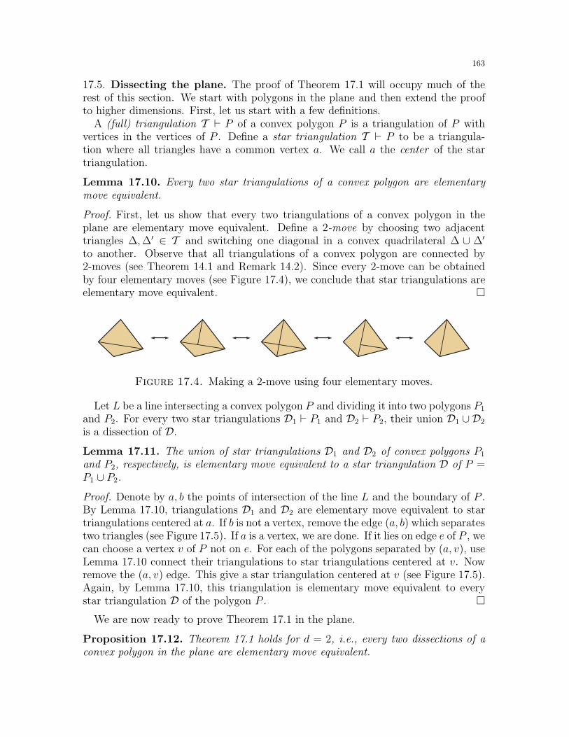
163

17.5. Dissecting the plane. The proof of Theorem 17.1 will occupy much of therest of this section. We start with polygons in the plane and then extend the proofto higher dimensions. First, let us start with a few definitions.

A (full) triangulation T ⊢ P of a convex polygon P is a triangulation of P withvertices in the vertices of P . Define a star triangulation T ⊢ P to be a triangula-tion where all triangles have a common vertex a. We call a the center of the startriangulation.

Lemma 17.10. Every two star triangulations of a convex polygon are elementarymove equivalent.

Proof. First, let us show that every two triangulations of a convex polygon in theplane are elementary move equivalent. Define a 2-move by choosing two adjacenttriangles ∆,∆′ ∈ T and switching one diagonal in a convex quadrilateral ∆ ∪ ∆′

to another. Observe that all triangulations of a convex polygon are connected by2-moves (see Theorem 14.1 and Remark 14.2). Since every 2-move can be obtainedby four elementary moves (see Figure 17.4), we conclude that star triangulations areelementary move equivalent.

Figure 17.4. Making a 2-move using four elementary moves.

Let L be a line intersecting a convex polygon P and dividing it into two polygons P1

and P2. For every two star triangulations D1 ⊢ P1 and D2 ⊢ P2, their union D1 ∪ D2

is a dissection of D.

Lemma 17.11. The union of star triangulations D1 and D2 of convex polygons P1

and P2, respectively, is elementary move equivalent to a star triangulation D of P =P1 ∪ P2.

Proof. Denote by a, b the points of intersection of the line L and the boundary of P .By Lemma 17.10, triangulations D1 and D2 are elementary move equivalent to startriangulations centered at a. If b is not a vertex, remove the edge (a, b) which separatestwo triangles (see Figure 17.5). If a is a vertex, we are done. If it lies on edge e of P , wecan choose a vertex v of P not on e. For each of the polygons separated by (a, v), useLemma 17.10 connect their triangulations to star triangulations centered at v. Nowremove the (a, v) edge. This give a star triangulation centered at v (see Figure 17.5).Again, by Lemma 17.10, this triangulation is elementary move equivalent to everystar triangulation D of the polygon P .

We are now ready to prove Theorem 17.1 in the plane.

Proposition 17.12. Theorem 17.1 holds for d = 2, i.e., every two dissections of aconvex polygon in the plane are elementary move equivalent.

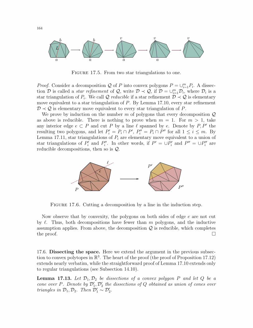
164

vvvbb

L

a aaa

Figure 17.5. From two star triangulations to one.

Proof. Consider a decomposition Q of P into convex polygons P = ∪mi=1Pi. A dissec-tion D is called a star refinement of Q, write D ≺ Q, if D = ∪mi=1Di, where Di is astar triangulation of Pi. We call Q reducible if a star refinement D ≺ Q is elementarymove equivalent to a star triangulation of P . By Lemma 17.10, every star refinementD ≺ Q is elementary move equivalent to every star triangulation of P .

We prove by induction on the number m of polygons that every decomposition Qas above is reducible. There is nothing to prove when m = 1. For m > 1, takeany interior edge e ⊂ P and cut P by a line ℓ spanned by e. Denote by P, P ′ theresulting two polygons, and let P ′

i = Pi ∩ P ′, P ′′i = Pi ∩ P ′′ for all 1 ≤ i ≤ m. By

Lemma 17.11, star triangulations of Pi are elementary move equivalent to a union ofstar triangulations of P ′

i and P ′′i . In other words, if P ′ = ∪P ′

i and P ′′ = ∪P ′′i are

reducible decompositions, then so is Q.

P

ℓ

e

P ′′

P ′

Figure 17.6. Cutting a decomposition by a line in the induction step.

Now observe that by convexity, the polygons on both sides of edge e are not cutby ℓ. Thus, both decompositions have fewer than m polygons, and the inductiveassumption applies. From above, the decomposition Q is reducible, which completesthe proof.

17.6. Dissecting the space. Here we extend the argument in the previous subsec-tion to convex polytopes in R3. The heart of the proof (the proof of Proposition 17.12)extends nearly verbatim, while the straightforward proof of Lemma 17.10 extends onlyto regular triangulations (see Subsection 14.10).

Lemma 17.13. Let D1,D2 be dissections of a convex polygon P and let Q be acone over P . Denote by D′

1,D′2 the dissections of Q obtained as union of cones over

triangles in D1,D2. Then D′1 ∼ D′

2.

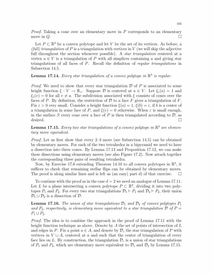
165

Proof. Taking a cone over an elementary move in P corresponds to an elementarymove in Q.

Let P ⊂ R3 be a convex polytope and let V be the set of its vertices. As before, a(full) triangulation of P is a triangulation with vertices in V (we will skip the adjectivefull throughout the section whenever possible). A star triangulation centered at avertex a ∈ V is a triangulation of P with all simplices containing a and giving startriangulations of all faces of P . Recall the definition of regular triangulations inSubsection 14.5.

Lemma 17.14. Every star triangulation of a convex polytope in R3 is regular.

Proof. We need to show that every star triangulation D of P is associated to someheight function ξ : V → R+. Suppose D is centered at a ∈ V . Let ξ(a) = 1 andξ(v) = 0 for all v 6= a. The subdivision associated with ξ consists of cones over thefaces of P . By definition, the restriction of D to a face F gives a triangulation of F .Fix ε > 0 very small. Consider a height function ξ(a) = 1, ξ(b) = ε, if b is a center ofa triangulation in some face of P , and ξ(v) = 0 otherwise. When ε is small enough,in the surface S every cone over a face of P is then triangulated according to D, asdesired.

Lemma 17.15. Every two star triangulations of a convex polytope in R3 are elemen-tary move equivalent.

Proof. Let us first show that every 2–3 move (see Subsection 14.5) can be obtainedby elementary moves. For each of the two tetrahedra in a bipyramid we need to havea dissection into three cones. By Lemma 17.13 and Proposition 17.12, we can makethese dissections using elementary moves (see also Figure 17.2). Now attach togetherthe corresponding three pairs of resulting tetrahedra.

Now, by Exercise 17.6 extending Theorem 14.10 to all convex polytopes in R3, itsuffices to check that remaining stellar flips can be obtained by elementary moves.The proof is along similar lines and is left as (an easy) part d) of that exercise.

To continue with the proof as in the case d = 2 we need an analogue of Lemma 17.11.Let L be a plane intersecting a convex polytope P ⊂ R3, dividing it into two poly-topes P1 and P2. For every two star triangulations D1 ⊢ P1 and D2 ⊢ P2, their unionD1 ∪ D2 is a dissection of D.

Lemma 17.16. The union of star triangulations D1 and D2 of convex polytopes P1

and P2, respectively, is elementary move equivalent to a star triangulation D of P =P1 ∪ P2.

Proof. The idea is to combine the approach in the proof of Lemma 17.11 with theheight function technique as above. Denote by A the set of points of intersection of Land edges in P . Fix a point a ∈ A, and denote by D the star triangulation of P withvertices in V ∪ A, centered at a and such that the center of triangulation of everyface lies on L. By construction, the triangulation D is a union of star triangulationsof P1 and P2, which are elementary move equivalent to D1 and D2 by Lemma 17.15.

166

Now, suppose L intersects face F ⊂ P , a /∈ F , by an edge (b, c). The cone from aover F is a dissection, which, by Lemma 17.13, is elementary move equivalent to astar triangulation with vertices in V ∪ A r b, c (see Figure 17.7). Repeating thisover every such face F we obtain a star triangulation D of P centered at a and withvertices in V ∪ a.

FF

ℓ

aa

b

c

Figure 17.7. star triangulation of a cone over F (view from the bottom).

Finally, let us use the height function approach to show that D is elementary moveequivalent to a star triangulation of P with vertices in V . Suppose a lies on theedge (v, w). Take the height function ξ : V ∪ a → R+ defined in the proof ofLemma 17.14. Recall that ξ(a) = 1 and ξ(v), ξ(w) > 0 are small. Continue as inthe proof of Theorem 14.10. Start increasing the values of v and w generically, untilξ(v), ξ(w) > 1, when a is no longer a vertex in a triangulation. Other than 2–3 moves,at some point, when ξ is linear on (v, w) a single elementary move will be used once,when the height function ξ is linear on (v, w). Note that the resulting triangulationis full, but not necessarily a star triangulation. By Theorem 14.10, we can connect itto a star triangulation by a sequence of 2–3 moves, which implies the result.

Proposition 17.17. Theorem 17.1 holds for d = 3, i.e., every two dissections of aconvex polytope in R3 are elementary move equivalent.

As we mentioned above, the proof follows from the lemmas above and the sameinductive argument.

Remark 17.18. As we mentioned in Remark 14.9, it is an open problem whether allfull triangulations of a convex polytope in R3 are connected by 2–3 moves [San2]. Thecorresponding result in dimensions 5 and higher is false. On the other hand, the graph ofall regular triangulations is not only connected, but is a graph of a convex polytope (seeExample 8.5 for a special case).

17.7. Wait, there is more! Yes, indeed. Remember we only proved the elementarymove connectivity theorem (Theorem 17.1) in the plane and in 3-dimensional space.In higher dimensions the proof follows roughly the same lines as long as one definesstar triangulation in higher dimension (see Exercise 17.1). As a consolation prize, weprove that the following generalization follows easily from Theorem 17.1.

167

Theorem 17.19. For every (possibly non-convex) polytope P ⊂ Rd, every two dis-sections D,D′ ⊢ P are elementary move equivalent: D ↔ D′.

Here by a polytope we mean any finite union of convex polytopes. Note that weimplicitly used convexity, for example, in the proof of the induction step in Propo-sition 17.12. Interestingly, the reduction to convex polytopes is now completelystraightforward.

Proof of Theorem 17.19. Take the intersection of the dissections (i.e., superimposethem as decompositions). We obtain a decomposition into convex polytopes. Refinethis decomposition by triangulating each polytope and denote by D the resultingdissection of P . Now observe that every simplex ∆ in D is connected by elementarymoves to its dissection in D. Therefore, D is elementary move equivalent to D, andwe conclude: D ↔ D ↔ D′.

17.8. Exercises.

Exercise 17.1. ♦ [1+] Finish the proof of Theorem 17.1 by extending the proof in Subsec-tion 17.6 to higher dimensions.

Exercise 17.2. [1-] Show that Exercise 16.24 is a simple corollary of Sydler’s theorem(Theorem 17.7). More generally, show that Sydler’s theorem implies that all polytopeswith rational dihedral angles are rectifiable.

Exercise 17.3. ♦ a) [1] Suppose ∆ and Q are as in Example 17.8. As in the example,assume that ∆ ∼ Q and consider the decompositions into tetrahedra proving this. Checkthat it suffices define the additive function f only on the (finitely many) dihedral anglesthat appear in the decomposition and obtain a contradiction.b) [1+] Prove existence of the additive functions f in Example 17.8.

Exercise 17.4. (Tverberg’s theorem) Let P ⊂ R3 be a convex polytope. Suppose we areallowed to cut P with a plane. Two parts are then separated, and each is then allowed tobe separately cut with a new plane, etc.43

a) [1-] Prove that a regular octahedron can be cut into tetrahedral pieces with only threecuts. Similarly, prove that for a cube four cuts suffice.b) [1-] Prove by an explicit construction that both regular icosahedron and regular dodec-ahedron need at most 100 cuts.c) [1] Prove that every convex polytope in R3 can be cut into tetrahedral pieces with finitelymany cuts.d) [1+] Generalize this to Rd.

Exercise 17.5. a) ♦ [1-] Let Q = ∂A be a simple polygon in R2. Prove that everytriangulation of A contains a triangle T with two sides in Q, i.e., such that A r T ishomeomorphic to a disk.b) [1+] In the plane, prove that for every decomposition Q = ∪iQi of a simply connectedpolygon Q into simply connected polygons Qi, there exist Qi such that QrQi is also simplyconnected.c) [1+] Show that part b) does not generalize to R3.

43Think of chopping polytopes as if they were vegetables.

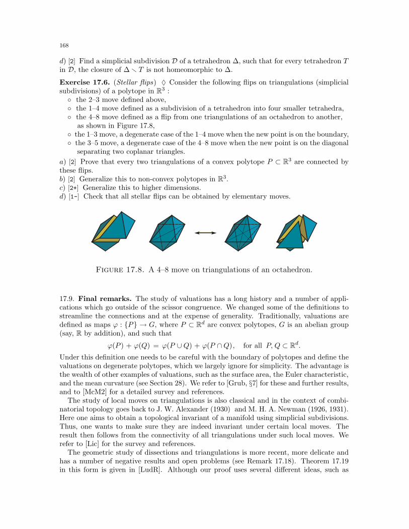
168

d) [2] Find a simplicial subdivision D of a tetrahedron ∆, such that for every tetrahedron Tin D, the closure of ∆r T is not homeomorphic to ∆.

Exercise 17.6. (Stellar flips) ♦ Consider the following flips on triangulations (simplicialsubdivisions) of a polytope in R3 : the 2–3 move defined above, the 1–4 move defined as a subdivision of a tetrahedron into four smaller tetrahedra, the 4–8 move defined as a flip from one triangulations of an octahedron to another,

as shown in Figure 17.8, the 1–3 move, a degenerate case of the 1–4 move when the new point is on the boundary, the 3–5 move, a degenerate case of the 4–8 move when the new point is on the diagonal

separating two coplanar triangles.

a) [2] Prove that every two triangulations of a convex polytope P ⊂ R3 are connected bythese flips.b) [2] Generalize this to non-convex polytopes in R3.c) [2+] Generalize this to higher dimensions.d) [1-] Check that all stellar flips can be obtained by elementary moves.

Figure 17.8. A 4–8 move on triangulations of an octahedron.

17.9. Final remarks. The study of valuations has a long history and a number of appli-cations which go outside of the scissor congruence. We changed some of the definitions tostreamline the connections and at the expense of generality. Traditionally, valuations aredefined as maps ϕ : P → G, where P ⊂ Rd are convex polytopes, G is an abelian group(say, R by addition), and such that

ϕ(P ) + ϕ(Q) = ϕ(P ∪Q) + ϕ(P ∩Q), for all P, Q ⊂ Rd.Under this definition one needs to be careful with the boundary of polytopes and define thevaluations on degenerate polytopes, which we largely ignore for simplicity. The advantage isthe wealth of other examples of valuations, such as the surface area, the Euler characteristic,and the mean curvature (see Section 28). We refer to [Grub, §7] for these and further results,and to [McM2] for a detailed survey and references.

The study of local moves on triangulations is also classical and in the context of combi-natorial topology goes back to J. W. Alexander (1930) and M. H. A. Newman (1926, 1931).Here one aims to obtain a topological invariant of a manifold using simplicial subdivisions.Thus, one wants to make sure they are indeed invariant under certain local moves. Theresult then follows from the connectivity of all triangulations under such local moves. Werefer to [Lic] for the survey and references.

The geometric study of dissections and triangulations is more recent, more delicate andhas a number of negative results and open problems (see Remark 17.18). Theorem 17.19in this form is given in [LudR]. Although our proof uses several different ideas, such as

169

height functions, the proofs share a similar blueprint. The triangulation counterpart of theelementary move connectivity theorem is also known, and uses the so-called stellar flipsor Pachner moves. These flips play an important role in both geometric combinatoricsand algebraic geometry. While many natural questions turn out to have negative answers,an important positive result (see Exercise 17.6) was established by Morelli (1996) andW lodarczyk (1997). We refer to [San2] for a survey of these result and to [IzmS] for anelegant presentation of the Morelli–W lodarczyk theorem.

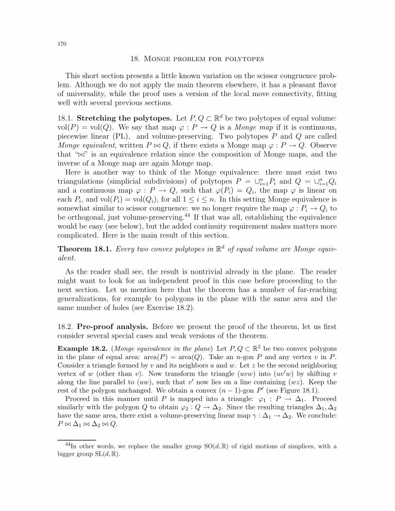
170

18. Monge problem for polytopes

This short section presents a little known variation on the scissor congruence prob-lem. Although we do not apply the main theorem elsewhere, it has a pleasant flavorof universality, while the proof uses a version of the local move connectivity, fittingwell with several previous sections.

18.1. Stretching the polytopes. Let P,Q ⊂ Rd be two polytopes of equal volume:vol(P ) = vol(Q). We say that map ϕ : P → Q is a Monge map if it is continuous,piecewise linear (PL), and volume-preserving. Two polytopes P and Q are calledMonge equivalent, written P ⊲⊳ Q, if there exists a Monge map ϕ : P → Q. Observethat “⊲⊳” is an equivalence relation since the composition of Monge maps, and theinverse of a Monge map are again Monge map.

Here is another way to think of the Monge equivalence: there must exist twotriangulations (simplicial subdivisions) of polytopes P = ∪ni=1Pi and Q = ∪ni=1Qi

and a continuous map ϕ : P → Q, such that ϕ(Pi) = Qi, the map ϕ is linear oneach Pi, and vol(Pi) = vol(Qi), for all 1 ≤ i ≤ n. In this setting Monge equivalence issomewhat similar to scissor congruence: we no longer require the map ϕ : Pi → Qi tobe orthogonal, just volume-preserving.44 If that was all, establishing the equivalencewould be easy (see below), but the added continuity requirement makes matters morecomplicated. Here is the main result of this section.

Theorem 18.1. Every two convex polytopes in Rd of equal volume are Monge equiv-alent.

As the reader shall see, the result is nontrivial already in the plane. The readermight want to look for an independent proof in this case before proceeding to thenext section. Let us mention here that the theorem has a number of far-reachinggeneralizations, for example to polygons in the plane with the same area and thesame number of holes (see Exercise 18.2).

18.2. Pre-proof analysis. Before we present the proof of the theorem, let us firstconsider several special cases and weak versions of the theorem.

Example 18.2. (Monge equivalence in the plane) Let P,Q ⊂ R2 be two convex polygonsin the plane of equal area: area(P ) = area(Q). Take an n-gon P and any vertex v in P .Consider a triangle formed by v and its neighbors u and w. Let z be the second neighboringvertex of w (other than v). Now transform the triangle (uvw) into (uv′w) by shifting valong the line parallel to (uw), such that v′ now lies on a line containing (wz). Keep therest of the polygon unchanged. We obtain a convex (n− 1)-gon P ′ (see Figure 18.1).

Proceed in this manner until P is mapped into a triangle: ϕ1 : P → ∆1. Proceedsimilarly with the polygon Q to obtain ϕ2 : Q → ∆2. Since the resulting triangles ∆1,∆2

have the same area, there exist a volume-preserving linear map γ : ∆1 → ∆2. We conclude:P ⊲⊳ ∆1 ⊲⊳ ∆2 ⊲⊳ Q.

44In other words, we replace the smaller group SO(d,R) of rigid motions of simplices, with abigger group SL(d,R).

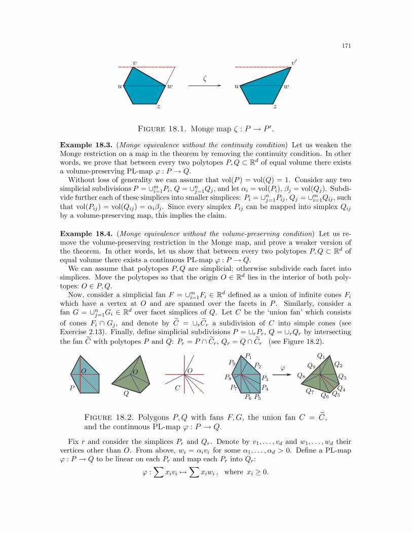
171

v

u uw w

z z

v′

ζ

Figure 18.1. Monge map ζ : P → P ′.

Example 18.3. (Monge equivalence without the continuity condition) Let us weaken theMonge restriction on a map in the theorem by removing the continuity condition. In otherwords, we prove that between every two polytopes P,Q ⊂ Rd of equal volume there existsa volume-preserving PL-map ϕ : P → Q.

Without loss of generality we can assume that vol(P ) = vol(Q) = 1. Consider any twosimplicial subdivisions P = ∪mi=1Pi, Q = ∪nj=1Qj , and let αi = vol(Pi), βj = vol(Qj). Subdi-vide further each of these simplices into smaller simplices: Pi = ∪nj=1Pij , Qj = ∪mi=1Qij, such

that vol(Pij) = vol(Qij) = αiβj . Since every simplex Pij can be mapped into simplex Qijby a volume-preserving map, this implies the claim.

Example 18.4. (Monge equivalence without the volume-preserving condition) Let us re-move the volume-preserving restriction in the Monge map, and prove a weaker version ofthe theorem. In other words, let us show that between every two polytopes P,Q ⊂ Rd ofequal volume there exists a continuous PL-map ϕ : P → Q.

We can assume that polytopes P,Q are simplicial; otherwise subdivide each facet intosimplices. Move the polytopes so that the origin O ∈ Rd lies in the interior of both poly-topes: O ∈ P,Q.

Now, consider a simplicial fan F = ∪mi=1Fi ∈ Rd defined as a union of infinite cones Fiwhich have a vertex at O and are spanned over the facets in P . Similarly, consider afan G = ∪nj=1Gi ∈ Rd over facet simplices of Q. Let C be the ‘union fan’ which consists

of cones Fi ∩ Gj , and denote by C = ∪rCr a subdivision of C into simple cones (seeExercise 2.13). Finally, define simplicial subdivisions P = ∪rPr, Q = ∪rQr by intersecting

the fan C with polytopes P and Q: Pr = P ∩ Cr, Qr = Q ∩ Cr (see Figure 18.2).

P1

P2

P3

P4

P5P6

P7

P8

P9

Q1

Q2

Q3

Q4Q5Q6

Q7

Q8

Q9ϕO OO

QP C

Figure 18.2. Polygons P,Q with fans F,G, the union fan C = C,and the continuous PL-map ϕ : P → Q.

Fix r and consider the simplices Pr and Qr. Denote by v1, . . . , vd and w1, . . . , wd theirvertices other than O. From above, wi = αivi for some α1, . . . , αd > 0. Define a PL-mapϕ : P → Q to be linear on each Pr and map each Pr into Qr:

ϕ :∑

xivi 7→∑

xiwi , where xi ≥ 0.

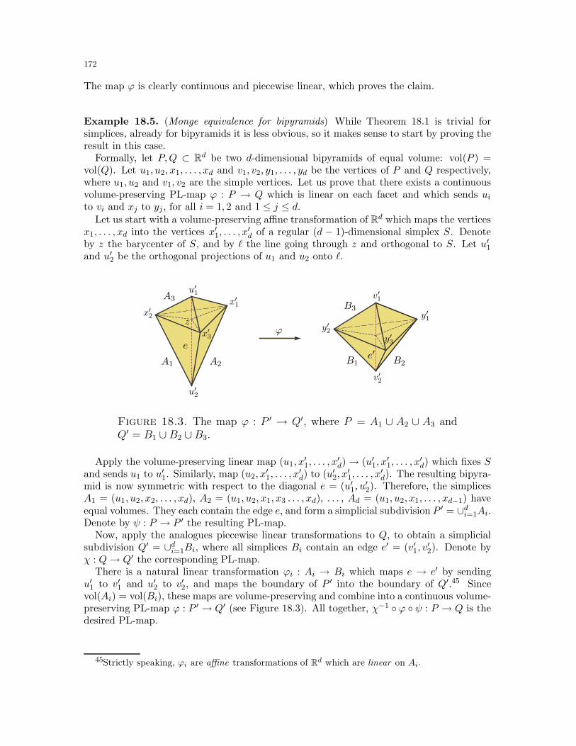
172

The map ϕ is clearly continuous and piecewise linear, which proves the claim.

Example 18.5. (Monge equivalence for bipyramids) While Theorem 18.1 is trivial forsimplices, already for bipyramids it is less obvious, so it makes sense to start by proving theresult in this case.

Formally, let P,Q ⊂ Rd be two d-dimensional bipyramids of equal volume: vol(P ) =vol(Q). Let u1, u2, x1, . . . , xd and v1, v2, y1, . . . , yd be the vertices of P and Q respectively,where u1, u2 and v1, v2 are the simple vertices. Let us prove that there exists a continuousvolume-preserving PL-map ϕ : P → Q which is linear on each facet and which sends uito vi and xj to yj , for all i = 1, 2 and 1 ≤ j ≤ d.

Let us start with a volume-preserving affine transformation of Rd which maps the verticesx1, . . . , xd into the vertices x′1, . . . , x

′d of a regular (d − 1)-dimensional simplex S. Denote

by z the barycenter of S, and by ℓ the line going through z and orthogonal to S. Let u′1and u′2 be the orthogonal projections of u1 and u2 onto ℓ.

A1 A2

A3

B1 B2

B3

ϕ

ee′

x′1x′2

x′3

u′1

u′2

y′1y′2

y′3

v′1

v′2

z

Figure 18.3. The map ϕ : P ′ → Q′, where P = A1 ∪ A2 ∪ A3 andQ′ = B1 ∪ B2 ∪B3.

Apply the volume-preserving linear map (u1, x′1, . . . , x

′d)→ (u′1, x

′1, . . . , x

′d) which fixes S

and sends u1 to u′1. Similarly, map (u2, x′1, . . . , x

′d) to (u′2, x

′1, . . . , x

′d). The resulting bipyra-

mid is now symmetric with respect to the diagonal e = (u′1, u′2). Therefore, the simplices

A1 = (u1, u2, x2, . . . , xd), A2 = (u1, u2, x1, x3 . . . , xd), . . . , Ad = (u1, u2, x1, . . . , xd−1) haveequal volumes. They each contain the edge e, and form a simplicial subdivision P ′ = ∪di=1Ai.Denote by ψ : P → P ′ the resulting PL-map.

Now, apply the analogues piecewise linear transformations to Q, to obtain a simplicialsubdivision Q′ = ∪di=1Bi, where all simplices Bi contain an edge e′ = (v′1, v

′2). Denote by

χ : Q→ Q′ the corresponding PL-map.There is a natural linear transformation ϕi : Ai → Bi which maps e → e′ by sending

u′1 to v′1 and u′2 to v′2, and maps the boundary of P ′ into the boundary of Q′.45 Sincevol(Ai) = vol(Bi), these maps are volume-preserving and combine into a continuous volume-preserving PL-map ϕ : P ′ → Q′ (see Figure 18.3). All together, χ−1 ϕ ψ : P → Q is thedesired PL-map.

45Strictly speaking, ϕi are affine transformations of Rd which are linear on Ai.

173

18.3. Monge maps by volume sharing. We are now ready to prove Theorem 18.1.Start with a continuous PL-map ϕ : P → Q constructed in Example 18.5. This mapcreates simplicial subdivisions P = ∪ni=1Pi, Q = ∪ni=1Qi, which will be fixed from hereon. For every i ∈ [n] compute ai = vol(Pi)/vol(Qi). If all ai = 1, the map ϕ is alsovolume-preserving, i.e., the Monge map is constructed. If not (which is more likely),let us “correct” map ϕ with a series of “local” PL-maps γ : Q→ Q.

Think of the numbers ai as contraction ratios of the linear maps ϕi : Pi → Qi.Formally, ai is the determinant of the inverse map at points in Qi. The maps weconstruct below will be continuous PL-maps ψ : P → Q which will have contractionratios bi at all points z ∈ Qi. In other words, the maps will neither be linear on Pi,nor take Pi to Qi. The maps we construct will be piecewise linear on all on Pi, andthe determinant of the inverse map ψ−1 will be a constant on Qi, for all i.

We begin with the obvious equation for the volume of simplices involved:

(£) vol(P ) =

n∑

i=1

ai · vol(Qi) =

n∑

i=1

vol(Qi).

Consider two adjacent simplices Qi and Qj and real numbers a′i, a′j such that

(U) ai · vol(Qi) + aj · vol(Qj) = a′i · vol(Qi) + a′j · vol(Qj).

Let us show how to construct a continuous PL-map ϕ′ : P → Q which is going tohave contraction ratios a′i and a′j on Qi and Qj, and unchanged contraction ratioselsewhere.

Suppose simplices Qi, Qj have a common face F . Expand the height of both sim-

plices by a factor of ai and aj , respectively. The resulting simplices Qi and Qj forma bipyramid A of volume

(ai · vol(Qi) + aj · vol(Qj)

). Similarly, expand the height of

both simplices by a factor of a′i and a′j , respectively, to obtain simplices Q′i and Q′

j

which form a bipyramid B of the same volume. Let Qij = Qi ∪ Qj , and denote byρ1 : Qij → A, ρ2 : Qij → B the two maps defined above. Let ζ : A→ B be a volume-preserving PL-map between these two bipyramids constructed in Example 18.5.

Now, let γ : Qij → Qij be defined as the composition γ = ρ−12 ζ ρ1 and extend γ

to a PL-map Q → Q by the identity map outside of the bipyramid Qij . This ispossible since the map ζ in the example was linear on the corresponding faces of thebipyramids (see Figure 18.4). Finally, let ϕ′ = ϕ γ. By construction, ϕ−1 = (ϕ′)−1

outside of Qij, and the contraction ratios on Qi and Qj are now a′i and a′j because ζis volume-preserving and ρ1 and ρ2 expand by exactly these factors.

Now that we know how to change the contraction ratios locally, let us make theglobal change. Loosely speaking, we claim that we can make local changes as in (U)to obtain a change as in the second equality in (£). Formally, consider a set A ofall sequences (a1, . . . , an) such that

∑i aivol(Qi) = vol(Q) and ai > 0. Let E be

the set of pairs (i, j) such that simplex Qi is adjacent to Qj (the intersection is a(d− 1)-dimensional face). We are allowed to change

(. . . , ai, . . . , aj, . . . ) → (. . . , a′i, . . . , a′j , . . . ) whenever (U) is satisfied.

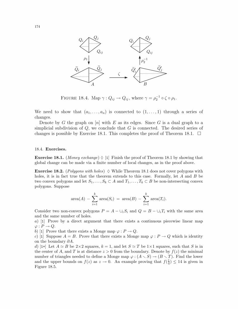
174

QiQiQjQj

Qi Qj Q′i

Q′j

QijQij

ζ

ρ1 ρ−12

A B

Figure 18.4. Map γ : Qij → Qij , where γ = ρ−12 ζ ρ1.

We need to show that (a1, . . . , an) is connected to (1, . . . , 1) through a series ofchanges.

Denote by G the graph on [n] with E as its edges. Since G is a dual graph to asimplicial subdivision of Q, we conclude that G is connected. The desired series ofchanges is possible by Exercise 18.1. This completes the proof of Theorem 18.1.

18.4. Exercises.

Exercise 18.1. (Money exchange) ♦ [1] Finish the proof of Theorem 18.1 by showing thatglobal change can be made via a finite number of local changes, as in the proof above.

Exercise 18.2. (Polygons with holes) ♦ While Theorem 18.1 does not cover polygons withholes, it is in fact true that the theorem extends to this case. Formally, let A and B betwo convex polygons and let S1, . . . , Sk ⊂ A and T1, . . . , Tk ⊂ B be non-intersecting convexpolygons. Suppose

area(A) −k∑

i=1

area(Si) = area(B) −k∑

i=1

area(Ti).

Consider two non-convex polygons P = A − ∪iSi and Q = B − ∪iTi with the same areaand the same number of holes.a) [1] Prove by a direct argument that there exists a continuous piecewise linear mapϕ : P → Q.b) [1] Prove that there exists a Monge map ϕ : P → Q.c) [1] Suppose A = B. Prove that there exists a Monge map ϕ : P → Q which is identityon the boundary ∂A.d) [1+] Let A ≃ B be 2×2 squares, k = 1, and let S ≃ T be 1×1 squares, such that S is inthe center of A, and T is at distance z > 0 from the boundary. Denote by f(z) the minimalnumber of triangles needed to define a Monge map ϕ : (Ar S)→ (B r T ). Find the lowerand the upper bounds on f(z) as z → 0. An example proving that f(1

4) ≤ 14 is given inFigure 18.5.

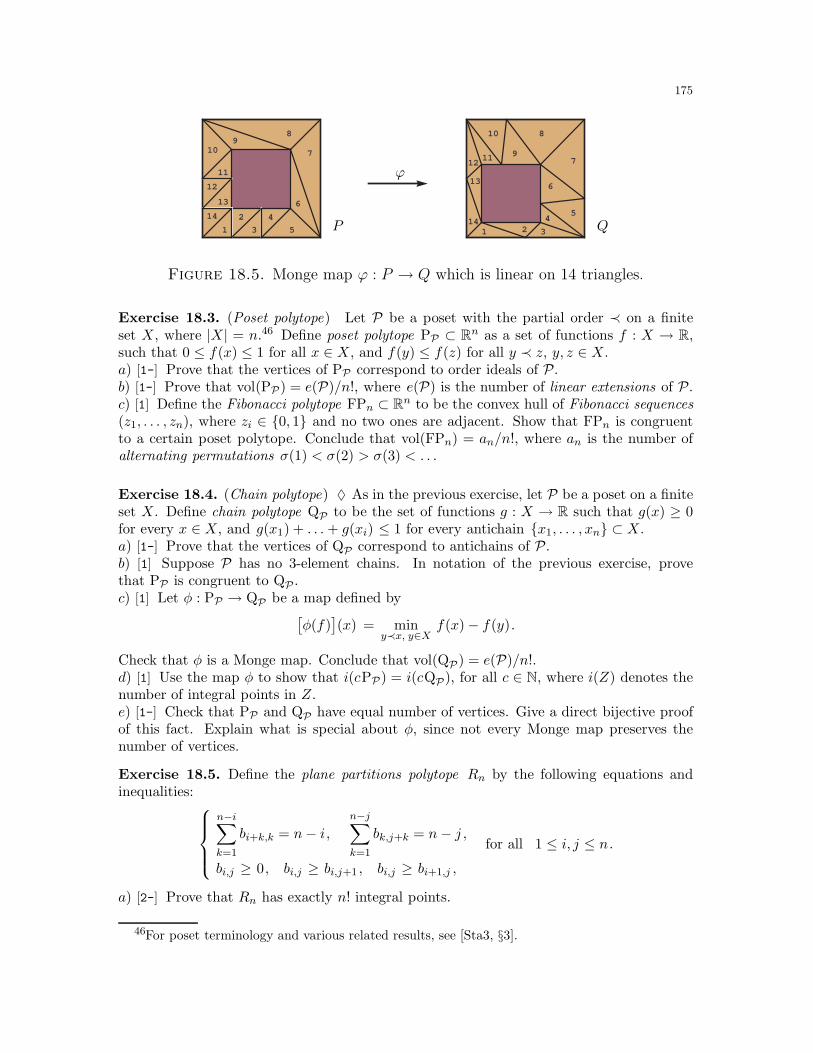
175

xxxxxxxxxxxxxxxxxxxxxxxxxxxxxxxxxxxxxxxxxxxxxxxxxxxxxxxxxxxxxxxxxxxxxxxxxxxxxxxxxxxxxxxxxxxxxxxxxxxxxxxxxxxxxxxxxxxxxxxxxxxxxxxxxxxxxxxxxxxxxxxxxxxxxxxxxxxxxxxxxxxxxxxxxxxxxxxxxxxxxxxxxxxxxxxxxxxxxxxxxxxxxxxxxxxxxxxxxxxxxxxxxxxxxxxxxxxxxxxxxxxxxxxxxxxxxxxxxxxxxxxxxxxxxxxxxxxxxxxxxxxxxxxxxxxxxxxxxxxxxxxxxxxxxxxxxxxxxxxxxxxxxxxxxxxxxxxxxxxxxxxxxxxxxxxxxxxxxxxxxxxxxxxxxxxxxxxxxxxxxxxxxxxxxxxxxxxxxxxxxxxxxxxxxxxxxxxxxxxxxxxxxxxxxxxxxxxxxxxxxxxxxxxxxxxxxxxxxxxxxx

xxxxxxxxxxxxxxxxxxxxxx

xxxxxxxxxxxxxxxxxxxxxxxxxxxxxxxxxxxxxxxxxxxxxxxxxxxxxxxxxxxxxxxxxxxxxxxxxxxxxxxxxxxxxxxxxxxxxxxxxxxxxxxxxxxxxxxxxxxxxxxxxxxxxxxxxxxxxxxxxxxxxxxxxxxxxxxxxxxxxxxxxxxxxxxxxxxxxxxxxxxxxxxxxxxxxxxxxxxxxxxxxxxxxxxxxxxxxxxxxxxxxxxxxxxxxxxxxxxxxxxxxxxxxxxxxxxxxxxxxxxxxxxxxxxxxxxxxxxxxxxxxxxxxxxxxxxxxxxxxxxxxxxxxxxxxxxxxxxxxxxxxxxxxxxxxxxxxxxxxxxxxxxxxxxxxxxxxxxxxxxxxxxxxxxxxxxxxxxxxxxxxxxxxxxxxxxxxxxxxxxxxxxxxxxxxxxxxxxxxxxxxxxxxxxxxxxxxxxxxxxxxxxxxxxxxxxxxxxxxxxxxxxxxxxxxxxxxxxxxxxxxxxx

xxxxxxxxxxxxxxxxxxxxxx

xxxxxxxxxxxxxxxxxxxxxxxxxxxxxxxxxxxxxxxxxxxxxxxxxxxxxxxxxxxxxxxxxxxxxxxxxxxxxxxxxxxxxxxxxxxxxxxxxxxxxxxxxxxxxxxxxxxxxxxxxxxxxxxxxxxxxxxxxxxxxxxxxxxxxxxxxxxxxxxxxxxxxxxxxxxxxxxxxxxxxxxxxxxxxxxxxxxxxxxxxxxxxxxxxxxxxxxxxxxxxxxxxxxxxxxxxxxxxxxxxxxxxxxxxxxxxxxxxxxxxxxxxxxxxxxxxxxxxxxxxxxxxxxxxxxxxxxxxxxxxxxxxxxxxxxxxxxxxxxxxxxxxxxxxxxxxxxxxxxxxxxxxxxxxxxxxxxxxxxxxxxxxxxxxxxxxxxxxxxxxxxxxxxxxxxxxxxxxxxxxxxxxxxxxxxxxxxxxxxxxxxxxxxxxxxxxxxxxxxxxxxxxxxxxxxxxxxxxxxxxx

xxxxxxxxxxxxxxxxxxxxxxxxxxxxxxxxxxxxxxxxxxxxxxxxxxxxxxxxxxxxxxxxxxxxxxxxxxxxxxxxxxxxxxxxxxxxxxxxxxxxxxxxxxxxxxxxxxxxxxxxxxxxxxxxxxxxxxxxxxxxxxxxxxxxxxxxxxxxxxxxxxxxxxxxxxxxxxxxxxxxxxxxxxxxxxxxxxxxxxxxxxxxxxxxxxxxxxxxxxxxxxxxxxxxxxxxxxxxxxxxxxxxxxxxxxxxxxxxxxxxxxxxxxxxxxxxxxxxxxxxxxxxxxxxxxxxxxxxxxxxxxxxxxxxxxxxxxxxxxxxxxxxxxxxxxxxxxxxxxxxxxxxxxxxxxxxxxxxxxxxxxxxxxxxxxxxxxxxxxxxxxxxxxxxxxxxxxxxxxxxxxxxxxxxxxxxxxxxxxxxxxxxxxxxxxxxxxxxxxxxxxxxxxxxxxxxxxxxxxxxxxxxxxxxxxxxxxxxxxxxxxxx

xxxxxxxxxxxxxxxxxxxxxxxxxxxxxxxxxxxxxxxxxxxxxxxxxxxxxxxxxxxxxxxxxxxxxxxxxxxxxxxxxxxxxxxxxxxxxxxxxxxxxxxxxxxxxxxxxxxxxxxxxxxxxxxxxxxxxxxxxxxxxxxxxxxxxxxxxxxxxxxxxxxxxxxxxxxxxxxxxxxxxxxxxxxxxxxxxxxxxxxxxxxxxxxxxxxxxxxxxxxxxxxxxxxxxxxxxxxxxxxxxxxxxxxxxxxxxxxxxxxxxxxxxxxxxxxxxxxxxxxxxxxxxxxxxxxxxxxxxxxxxxxxxxxxxxxxxxxxxxxxxxxxxxxxxxxxxxxxxxxxxxxxxxxxxxxxxxxxxxxxxxxxxxxxxxxxxxxxxxxxxxxxxxxxxxxxxxxxxxxxxxxxxxxxxxxxxxxxxxxxxxxxxxxxxxxxxxxxxxxxxxxxxxxxxxxxxxxxxxxxxxxxxxxxxxxxxxxxxxxxxxxxxxxxxxxxxxxxxxxxxxxxxxxxxxxxxxxxxxxxxxxxxxxxxxxxxxxxxxxxxxxxxxxxxxxxxxxxxxxxxxxxxxxxxxxxxxxxxxxxxxxxxxxxxxxxxxxxxxxxxxxxxxxxxxxxxxxxxxxxxxxxxxxxxxxxxxxxxxxxxxxxxxxxxxxxxxxxxxxxxxxxxxxxxxxxxxxxxxxxxxxxxxxxxxxxxxxxxxxxxxxxxxxxxxxxxxxxxxxxxxxxxxxxxxxxxxxxxxxxxxxxxxxxxxxxxxxxxxxxxxxxxxxxxxxxxxxxxxxxxxxxxxxxxxxxxxxxxxxxxxxxxxxxxxxxxxxxxxxxxxxxxxxxxxxxxxxxxxxxxxxxxxxxxxxxxxxxxxxxxxxxxxxxxxxxxxxxxxxxxxxxxxxxxxxxxxxxxxxxxxxxxxxxxxxxxxxxxxxxxxxxxxxxxxxxxxxxxxxxxxxxxxxxxxxxxxxxxxxxxxxxxxxxxxxxxxxxxxxxxxxxxxxxxxxxxxxxxxxxxxxxxxxxxxxxxxxxxxxxxxxxxxxxxxxxxxxxxxxxxxxxxxxxxxxxxxxxxxxxxxxxxxxxxxxxxxxxxxxxxxxxxxxxxxxxxxxxxxxxxxxxxxxxxxxxxxxxxxxxxxxxxxxxxxxxxxxxxxxxxxxxxxxxxxxxxxxxxxxxxxxxxxxxxxxxxxxxxxxxxxxxxxxxxxxxxxxxxxxxxxxxxxxxxxxxxxxxxxxxxxxxxxxxxxxxxxxxxxxxxxxxxxxxxxxxxxxxxxxxxxxxxxxxxxxxxxxxxxxxxxxxxxxxxxxxxxxxxxxxxxxxxxxxxxxxxxxxxxxxxxxxxxxxxxxxxxxxxxxxxxxxxxxxxxxxxxxxxxxxxxxxxxxxxxxxxxxxxxxxxxxxxxxxxxxxxxxxxxxxxxxxxxxxxxxxxxxxxxxxxxxxxxxxxxxxxxxxxxxxxxxxxxxxxxxxxxxxxxxxxxxxxxxxxxxxxxxxxxxxxxxxxxxxxxxxxxxxxxxxxxxxxxxxxxxxxxxxxxxxxxxxxxxxxxxxxxxxxxxxxxxxxxxxxxxxxxxxxxxxxxxxxxxxxxxxxxxxxxxxxxxxxxxxxxxxxxxxxxxxxxxxxxxxxxxxxxxxxxxxxxxxxxxxxxxxxxxxxxxxxxxxxxxxxxxxxxxxxxxxxxxxxxxxxxxxxxxxxxxxxxxxxxxxxxxxxxxxxxxxxxxxxxxxxxxxxxxxxxxxxxxxxxxxxxxxxxxxxxxxxxxxxxxxxxxxxxxxxxxxxxxxxxxxxxxxxxxxxxxxxxxxxxxxxxxxxxxxxxxxxxxxxxxxxxxxxxxxxxxxxxxxxxxxxxxxxxxxxxxxxxxxxxxx

xxxxxxxxxxxxxxxxxxxxxxxxxxxxxxxxxxxxxxxxxxxxxxxxxxxxxxxxxxxxxxxxxxxxxxxxxxxxxxxxxxxxxxxxxxxxxxxxxxxxxxxxxxxxxxxxxxxxxxxxxxxxxxxxxxxxxxxxxxxxxxxxxxxxxxxxxxxxxxxxxxxxxxxxxxxxxxxxxxxxxxxxxxxxxxxxxxxxxxxxxxxxxxxxxxxxxxxxxxxxxxxxxxxxxxxxxxxxxxxxxxxxxxxxxxxxxxxxxxxxxxxxxxxxxxxxxxxxxxxxxxxxxxxxxxxxxxxxxxxxxxxxxxxxxxxxxxxxxxxxxxxxxxxxxxxxxxxxxxxxxxxxxxxxxxxxxxxxxxxxxxxxxxxxxxxxxxxxxxxxxxxxxxxxxxxxxxxxxxxxxxxxxxxxxxxxxxxxxxxxxxxxxxxxxxxxxxxxxxxxxxxxxxxxxxxxxxxxxxxxxxxxxxxxxxxxxxxxxxxxxxxxxxxxxxxxxxxxxxxxxxxxxxxxxxxxxxxxxxxxxxxxxxxxxxxxxxxxxxxxxxxxxxxxxxxxxxxxxxxxxxxxxxxxxxxxxxxxxxxxxxxxxxxxxxxxxxxxxxxxxxxxxxxxxxxxxxxxxxxxxxxxxxxxxxxxxxxxxxxxxxxxxxxxxxxxxxxxxxxxxxxxxxxxxxxxxxxxxxxxxxxxxxxxxxxxxxxxxxxxxxxxxxxxxxxxxxxxxxxxxxxxxxxxxxxxxxxxxxxxxxxxxxxxxxxxxxxxxxxxxxxxxxxxxxxxxxxxxxxxxxxxxxxxxxxxxxxxxxxxxxxxxxxxxxxxxxxxxxxxxxxxxxxxxxxxxxxxxxxxxxxxxxxxxxxxxxxxxxxxxxxxxxxxxxxxxxxxxxxxxxxxxxxxxxxxxxxxxxxxxxxxxxxxxxxxxxxxxxxxxxxxxxxxxxxxxxxxxxxxxxxxxxxxxxxxxxxxxxxxxxxxxxxxxxxxxxxxxxxxxxxxxxxxxxxxxxxxxxxxxxxxxxxxxxxxxxxxxxxxxxxxxxxxxxxxxxxxxxxxxxxxxxxxxxxxxxxxxxxxxxxxxxxxxxxxxxxxxxxxxxxxxxxxxxxxxxxxxxxxxxxxxxxxxxxxxxxxxxxxxxxxxxxxxxxxxxxxxxxxxxxxxxxxxxxxxxxxxxxxxxxxxxxxxxxxxxxxxxxxxxxxxxxxxxxxxxxxxxxxxxxxxxxxxxxxxxxxxxxxxxxxxxxxxxxxxxxxxxxxxxxxxxxxxxxxxxxxxxxxxxxxxxxxxxxxxxxxxxxxxxxxxxxxxxxxxxxxxxxxxxxxxxxxxxxxxxxxxxxxxxxxxxxxxxxxxxxxxxxxxxxxxxxxxxxxxxxxxxxxxxxxxxxxxxxxxxxxxxxxxxxxxx

xxxxxxxxxxxxxxxxxxxxxxxxxxxxxxxxxxxxxxxxxxxxxxxxxxxxxxxxxxxxxxxxxxxxxxxxxxxxxxxxxxxxxxxxxxxxxxxxxxxxxxxxxxxxxxxxxxxxxxxxxxxxxxxxxxxxxxxxxxxxxxxxxxxxxxxxxxxxxxxxxxxxxxxxxxxxxxxxxxxxxxxxxxxxxxxxxxxxxxxxxxxxxxxxxxxxxxxxxxxxxxxxxxxxxxxxxxxxxxxxxxxxxxxxxxxxxxxxxxxxxxxxxxxxxxxxxxxxxxxxxxxxxxxxxxxxxxxxxxxxxxxxxxxxxxxxxxxxxxxxxxxxxxxxxxxxxxxxxxxxxxxxxxxxxxxxxxxxxxxxxxxxxxxxxxxxxxxxxxxxxxxxxxxxxxxxxxxxxxxxxxxxxxxxxxxxxxxxxxxxxxxxxxxxxxxxxxxxxxxxxxxxxxxxxxxxxxxxxxxxxxxxxxxxxxxxxxxxxxxxxxxxxxxxxxxxxxxxxxxxxxxxxxxxxxxxxxxxxxxxxxxxxxxxxxxxxxxxxxxxxxxxxxxxxxxxxxxxxxxxxxxxxxxxxxxxxxxxxxxxxxxxxxxxxxxxxxxxxxxxxxxxxxxxxxxxxxxxxxxxxxxxxxxxxxxxxxxxxxxxxxxxxxxxxxxxxxxxxxxxxxxxxxxxxxxxxxxxxxxxxxxxxxxxxxxxxxxxxxxxxxxxxxxxxxxxxxxxxxxxxxxxxxxxxxxxxxxxxxxxxxxxxxxxxxxxxxxxxxxxxxxxxxxxxxxxxxxxxxxxxxxxxxxxxxxxxxxxxxxxxxxxxxxxxxxxxxxxxxxxxxxxxxxxxxxxxxxxxxxxxxxxxxxxxxxxxxxxxxxxxxxxxxxxxxxxxxxxxxxxxxxxxxxxxxxxxxxxxxxxxxxxxxxxxxxxxxxxxxxxxxxxxxxxxxxxxxxxxxxxxxxxxxxxxxxxxxxxxxxxxxxxxxxxxxxxxxxxxxxxxxxxxxxxxxxxxxxxxxxxxxxxxxxxxxxxxxxxxxxxxxxxxxxxxxxxxxxxxxxxxxxxxxxxxxxxxxxxxxxxxxxxxxxxxxxxxxxxxxxxxxxxxxxxxxxxxxxxxxxxxxxxxxxxxxxxxxxxxxxxxxxxxxxxxxxxxxxxxxxxxxxxxxxxxxxxxxxxxxxxxxxxxxxxxxxxxxxxxxxxxxxxxxxxxxxxxxxxxxxxxxxxxxxxxxxxxxxxxxxxxxxxxxxxxxxxxxxxxxxxxxxxxxxxxxxxxxxxxxxxxxxxxxxxxxxxxxxxxxxxxxxxxxxxxxxxxxxxxxxxxx

1

2

3

4

5

6

7

89

10

11

12

13

14

xxxxxxxxxxxxxxxxxxxxxxxxxxxxxxxxxxxxxxxxxxxxxxxxxxxxxxxxxxxxxxxxxxxxxxxxxxxxxxxxxxxxxxxxxxxxxxxxxxxxxxxxxxxxxxxxxxxxxxxxxxxxxxxxxxxx

xxxxxxxxxxxxxxxxxxxxxxxxxxxxxxxxxxxxxxxxxxxxxxxxxxxxxxxxxxxxxxxxxxxxxxxxxxxxxxxxxxxxxxxxxxxxxxxxxxxxxxxxxxxxxxxxxxxxxxxxxxxxxxxxxxxxxxxxxxxxxxxxxxxxxxxxxxxxxxxxxxxxxxxxxxxxxxxxxxxxxxxxxxxxxxxxxxxxxxxxxxxxxxxxxxxxxxxxxxxxxxxxxxxxxxxxxxxxxxxxxxxxxxxxxxxxxxxxxxxxxxxxxxxxxxxxxxxxxxxxxxxxxxxxxxxxxxxxxxxxxxxxxxxxxxxxxxxxxxxxxxxxxxxxxxxxxxxxxxxxxxxxxxxxxxxxxxxxxxxxxxxxxxxxxxxxxxxxxxxxxxxx

xxxxxxxxxxxxxxxxxxxxxxxxxxxxxxxxxxxxxxxxxxxxxxxxxxxxxxxxxxxxxxxxxxxxxxxxxxxxxxxxxxxxxxxxxxxxxxxxxxxxxxxxxxxxxxxxxxxxxxxxxxxxxxxxxxxx

xxxxxxxxxxxxxxxxxxxxxxxxxxxxxxxxxxxxxxxxxxxxxxxxxxxxxxxxxxxxxxxxxxxxxxxxxxxxxxxxxxxxxxxxxxxxxxxxxxxxxxxxxxxxxxxxxxxxxxxxxxxxxxxxxxxxxxxxxxxxxxxxxxxxxxxxxxxxxxxxxxxxxxxxxxxxxxxxxxxxxxxxxxxxxxxxxxxxxxxxxxxxxxxxxxxxxxxxxxxxxxxxxxxxxxxxxxxxxxxxxxxxxxxxxxxxxxxxxxxxxxxxxxxxxxxxxxxxxxxxxxxxxxxxxxxxxxxxxxxxxxxxxxxxxxxxxxxxxxxxxxxxxxxxxxxxxxxxxxxxxxxxxxxxxxxxxxxxxxxxxxxxxxxxxxxxxxxxxxxxxxxx

xxxxxxxxxxxxxxxxxxxxxxxxxxxxxxxxxxxxxxxxxxxxxxxxxxxxxxxxxxxxxxxxxxxxxxxxxxxxxxxxxxxxxxxxxxxxxxxxxxxxxxxxxxxxxxxxxxxxxxxxxxxxxxxxxxxxxxxxxxxxxxxxxxxxxxxxxxxxxxxxxxxxxxxxxxxxxxxxxxxxxxxxxxxxxxxxxxxxxxxxxxxxxxxxxxxxxxxxxxxxxxxxxxxxxxxxxxxxxxxxxxxxxxxxxxxxxxxxxxxxxxxxxxxxxxxxxxxxxxxxxxxxxxxxxxxxxxxxxxxxxxxxxxxxxxxxxxxxxxxxxxxxxxxxxxxxxxxxxxxxxxxxxxxxxxxxxxxxxxxxxxxxxxxxxxxxxxxxxxxxxxxxxxxxxxxxxxxxxxxxxxxxxxxxxxxxxxxxxxxxxxxxxxxxxxxxxxxxxxxxxxxxxxxxxxxxxxxxxxxxxxxxxxxxxxxxxxxxxxxxxxxxxxxxxxxxxxxxxxxxxxxxxxxxxxxxxxxxxxxxxxxxxxxxxxxxxxxxxxxxxxxxxxxxxxxxxxxxxxxxxxxxxxxxxxxxxxxxxxxxxxxxxxxxxxxxxxxxxxxxxxxxxxxxxxxxxxxxxxxxxxxxxxxxxxxxxxxxxxxxxxxxxxxxxxxxxxxxxxxxxxxxxxxxxxxxxxxxxxxxxxxxxxxxxxxxxxxxxxxxxxxxxxxxxxxxxxxxxxxxxxxxxxxxxxxxxxxxxxxxxxxxxxxxxxxxxxxxxxxxxxxxxxxxxxxxxxxxxxxxxxxxxxxxxxxxxxxxxxxxxxxxxxxxxxxxxxxxxxxxxxxxxxxxxxxxxxxxxxxxxxxxxxxxxxxxxxxxxxxxxxxxxxxxxxxxxxxxxxxxxxxxxxxxxxxxxxxxxxxxxxxxxxxxxxxxxxxxxxxxxxxxxxxxxxxxxxxxxxxxxxxxxxxxxxxxxxxxxxxxxxxxxxxxxxxxxxxxxxxxxxxxxxxxxxxxxxxxxxxxxxxxxxxxxxxxxxxxxxxxxxxxxxxxxxxxxxxxxxxxxxxxxxxxxxxxxxxxxxxxxxxxxxxxxxxxxxxxxxxxxxxxxxxxxxxxxxxxxxxxxxxxxxxxxxxxxxxxxxxxxxxxxxxxxxxxxxxxxxxxxxxxxxxxxxxxxxxxxxxxxxxxxxxxxxxxxxxxxxxxxxxxxxxxxxxxxxxxxxxxxxxxxxxxxxxxxxxxxxxxxxxxxxxxxxxxxxxxxxxxxxxxxxxxxxxxxxxxxxxxxxxxxxxxxxxxxxxxxxxxxxxxxxxxxxxxxxxxxxxxxxxxxxxxxxxxxxxxxxxxxxxxxxxxxxxxxxxxxxxxxxxxxxxxxxxxxxxxxxxxxxxxxxxxxxxxxxxxxxxxxxxxxxxxxxxxxxxxxxxxxxxxxxxxxxxxxxxxxxxxxxxxxxxxxxxxxxxxxxxxxxxxxxxxxxxxxxxxxxxxxxxxxxxxxxxxxxxxxxxxxxxxxxxxxxxxxxxxxxxxxxxxxxxxxxxxxxxxxxxxxxxxxxxxxxxxxxxxxxxxxxxxxxxxxxxxxxxxxxxxxxxxxxxxxxxxxxxxxxxxxxxxxxxxxxxxxxxxxxxxxxxxxxxxxxxxxxxxxxxxxxxxxxxxxxxxxxxxxxxxxxxxxxxxxxxxxxxxxxxxxxxxxxxxxxxxxxxxxxxxxxxxxxxxxxxxxxxxxxxxxxxxxxxxxxxxxxxxxxxxxxxxxxxxxxxxxxxxxxxxxxxxxxxxxxxxxxxxxxxxxxxxxxxxxxxxxxxxxxxxxxxxxxxxxxxxxxxxxxxxxxxxxxxxxxxxxxxxxxxxxxxxxxxxxxxxxxxxxxxxxxxxxxxxxxxxxxxxxxxxxxxxxxxxxxxxxxxxxxxxxxxxxxxxxxxxxxxxxxxxxxxxxxxxxxxxxxxxxxxxxxxxxxxxxxxxxxxxxxxxxxxxxxxxxxxxxxxxxxxxxxxxxxxxxxxxxxxxxxxxxxxxxxxxxxxxxxxxxxxxxxxxxxxxxxxxxxxxxxxxxxxxxxxxxxxxxxxxxxxxxxxxxxxxxxxxxxxxxxxxxxxxxxxxxxxxxxxxxxxxxxxxxxxxxxxxxxxxxxxxxxxxxxxxxxxxxxxxxxxxxxxxxxxxxxxxxxxxxxxxxxxxxxxxxxxxxxxxxxxxxxxxxxxxxxxxxxxxxxxxxxxxxxxxxxxxxxxxxxxxxxxxxxxxxxxxxxxxxxxxxxxxxxxxxxxxxxxxxxxxxxxxxxxxxxxxxxxxxxxxxxxxxxxxxxxxxxxxxxxxxxxxxxxxxxxxxxxxxxxxxxxxxxxxxxxxxxxxxxxxxxxxxxxxxxxxxxxxxxxxxxxxxxxxxxxxxxxxxxxxxxxxxxxxxxxxxxxxxxxxxxxxxxxxxxxxxxxxxxxxxxxxxxxxxxxxxxxxxxxxxxxxxxxxxxxxxxxxxxxxxxxxxxxxxxxxxxxxxxxxxxxxxxxxxxxxxxxxxxxxxxxxxxxxxxxxxxxxxxxxxxxxxxxxxxxxxxxxxxxxxxxxxxxxxxxxxxxxxxxxxxxxxxxxxxxxxxxxxxxxxxxxxxxxxxxxxxxxxxxxxxxxxxxxxxxxxxxxxxxxxxxxxxxxxxxxxxxxxxxxxxxxxxxxxxxxxxxxxxxxxxxxxxxxxxxxxxxxxxxxxxxxxxxxxxxxxxxxxxxxxxxxxxxxxxxxxxxxxxxxxxxxxxxxxxxxxxxxxxxxxxxxxxxxxxxxxxxxxxxxxxxxxxxxxxxx

xxxxxxxxxxxxxxxxxxxxxxxxxxxxxxxxxxxxxxxxxxxxxxxxxxxxxxxxxxxxxxxxxxxxxxxxxxxxxxxxxxxxxxxxxxxxxxxxxxxxxxxxxxxxxxxxxxxxxxxxxxxxxxxxxxxxxxxxxxxxxxxxxxxxxxxxxxxxxxxxxxxxxxxxxxxxxxxxxxxxxxxxxxxxxxxxxxxxxxxxxxxxxxxxxxxxxxxxxxxxxxxxxxxxxxxxxxxxxxxxxxxxxxxxxxxxxxxxxxxxxxxxxxxxxxxxxxxxxxxxxxxxxxxxxxxxxxxxxxxxxxxxxxxxxxxxxxxxxxxxxxxxxxxxxxxxxxxxxxxxxxxxxxxxxxxxxxxxxxxxxxxxxxxxxxxxxxxxxxxxxxxxxxxxxxxxxxxxxxxxxxxxxxxxxxxxxxxxxxxxxxxxxxxxxxxxxxxxxxxxxxxxxxxxxxxxxxxxxxxxxxxxxxxxxxxxxxxxxxxxxxxxxxxxxxxxxxxxxxxxxxxxxxxxxxxxxxxxxxxxxxxxxxxxxxxxxxxxxxxxxxxxxxxxxxxxxxxxxxxxxxxxxxxxxxxxxxxxxxxxxxxxxxxxxxxxxxxxxxxxxxxxxxxxxxxxxxxxxxxxxxxxxxxxxxxxxxxxxxxxxxxxxxxxxxxxxxxxxxxxxxxxxxxxxxxxxxxxxxxxxxxxxxxxxxxxxxxxxxxxxxxxxxxxxxxxxxxxxxxxxxxxxxxxxxxxxxxxxxxxxxxxxxxxxxxxxxxxxxxxxxxxxxxxxxxxxxxxxxxxxxxxxxxxxxxxxxxxxxxxxxxxxxxxxxxxxx

xxxxxxxxxxxxxxxxxxxxxxxxxxxxxxxxxxxxxxxxxxxxxxxxxxxxxxxxxxxxxxxxxxxxxxxxxxxxxxxxxxxxxxxxxxxxxxxxxxxxxxxxxxxxxxxxxxxxxxxxxxxxxxxxxxxxxxxxxxxxxxxxxxxxxxxxxxxxxxxxxxxxxxxxxxxxxxxxxxxxxxxxxxxxxxxxxxxxxxxxxxxxxxxxxxxxxxxxxxxxxxxxxxxxxxxxxxxxxxxxxxxxxxxxxxxxxxxxxxxxxxxxxxxxxxxxxxxxxxxxxxxxxxxxxxxxxxxxxxxxxxxxxxxxxxxxxxxxxxxxxxxxxxxxxxxxxxxxxxxxxxxxxxxxxxxxxxxxxxxxxxxxxxxxxxxxxxxxxxxxxxxxxxxxxxxxxxxxxxxxxxxxxxxxxxxxxxxxxxxxxxxxxxxxxxxxxxxxxxxxxxxxxxxxxxxxxxxxxxxxxxxxxxxxxxxxxxxxxxxxxxxxxxxxxxxxxxxxxxxxxxxxxxxxxxxxxxxxxxxxxxxxxxxxxxxxxxxxxxxxxxxxxxxxxxxxxxxxxxxxxxxxxxxxxxxxxxxxxxxxxxxxxxxxxxxxxxxxxxxxxxxxxxxxxxxxxxxxxxxxxxxxxxxxxxxxxxxxxxxxxxxxxxxxxxxxxxxxxxxxxxxxxxxxxxxxxxxxxxxxxxxxxxxxxxxxxxxxxxxxxxxxxxxxxxxxxxxxxxxxxxxxxxxxxxxxxxxxxxxxxxxxxxxxxxxxxxxxxxxxxxxxxxxxxxxxxxx

xxxxxxxxxxxxxxxxxxxxxxxxxxxxxxxxxxxxxxxxxxxxxxxxxxxxxxxxxxxxxxxxxxxxxxxxxxxxxxxxxxxxxxxxxxxxxxxxxxxxxxxxxxxxxxxxxxxxxxxxxxxx

xxxxxxxxxxxxxxxxxxxxxxxxxxxxxxxxxxxxxxxxxxxxxxxxxxxxxxxxxxxxxxxxxxxxxxxxxxxxxxxxxxxxxxxxxxxxxxxxxxxxxxxxxxxxxxxxxxxxxxxxxxxxxxxxxxxxxxxxxxxxxxxxxxxxxxxxxxxxxxxxxxxxxxxxxxxxxxxxxxxxxxxxxxxxxxxxxxxxxxxxxxxxxxxxxxxxxxxxxxxxxxxxxxxxxxxxxxxxxxxxxxxxxxxxxxxxxxxxxxxxxxxxxxxxxxxxxxxxxxxxxxxxxxxxxxxxxxxxxxxxxxxxxxxxxxxxxxxxxxxxxxxxxxxxxxxxxxxxxxxxxxxxxxxxxxxxxxxxxxxxxxxxxxxxxxxxxxxxxxxxxxxxxxxxxxxxxxxxxxxxxxxxxxxxxxxxxxxxxxxxxxxxxxxxxxxxxxxxxxxxxxxxxxxxxxxxxxxxxxxxxxxxxxxxxxxxxxxxxxxxxxxxxxxxxxxxxxxxxxxxxxxxxxxxxxxxxxxxxxxxxxxxxxxxxxxxxxxxxxxxxxxxxxxxxxxxxxxxxxxxxxxxxxxxxxxxxxxxxxxxxxxxxxxxxxxxxxxxxxxxxxxxxxxxxxxxxxxxxxxxxxxxxxxxxxxxxxxxxxxxxxxxxxxxxxxxxxxxxxxxxxxxxxxxxxxxxxxxxxxxxxxxxxxxxxxxxxxxxxxxxxxxxxxxxxxxxxxxxxxxxxxxxxxxxxxxxxxxxxxxxxxxxxxxxxxxxxxxxxxxxxxxxxxxxxxxxxx

1 2 3

45

6

7

810

911

12

13

14

xxxxxxxxxxxxxxxxxxxxxxxxxxxxxxxxxxx

ϕ

P Q

Figure 18.5. Monge map ϕ : P → Q which is linear on 14 triangles.

Exercise 18.3. (Poset polytope) Let P be a poset with the partial order ≺ on a finiteset X, where |X| = n.46 Define poset polytope PP ⊂ Rn as a set of functions f : X → R,such that 0 ≤ f(x) ≤ 1 for all x ∈ X, and f(y) ≤ f(z) for all y ≺ z, y, z ∈ X.a) [1-] Prove that the vertices of PP correspond to order ideals of P.b) [1-] Prove that vol(PP) = e(P)/n!, where e(P) is the number of linear extensions of P.c) [1] Define the Fibonacci polytope FPn ⊂ Rn to be the convex hull of Fibonacci sequences(z1, . . . , zn), where zi ∈ 0, 1 and no two ones are adjacent. Show that FPn is congruentto a certain poset polytope. Conclude that vol(FPn) = an/n!, where an is the number ofalternating permutations σ(1) < σ(2) > σ(3) < . . .

Exercise 18.4. (Chain polytope) ♦ As in the previous exercise, let P be a poset on a finiteset X. Define chain polytope QP to be the set of functions g : X → R such that g(x) ≥ 0for every x ∈ X, and g(x1) + . . .+ g(xi) ≤ 1 for every antichain x1, . . . , xn ⊂ X.a) [1-] Prove that the vertices of QP correspond to antichains of P.b) [1] Suppose P has no 3-element chains. In notation of the previous exercise, provethat PP is congruent to QP .c) [1] Let φ : PP → QP be a map defined by

[φ(f)

](x) = min

y≺x, y∈Xf(x)− f(y).

Check that φ is a Monge map. Conclude that vol(QP ) = e(P)/n!.d) [1] Use the map φ to show that i(cPP) = i(cQP), for all c ∈ N, where i(Z) denotes thenumber of integral points in Z.e) [1-] Check that PP and QP have equal number of vertices. Give a direct bijective proofof this fact. Explain what is special about φ, since not every Monge map preserves thenumber of vertices.

Exercise 18.5. Define the plane partitions polytope Rn by the following equations andinequalities:

n−i∑

k=1

bi+k,k = n− i,n−j∑

k=1

bk,j+k = n− j ,

bi,j ≥ 0, bi,j ≥ bi,j+1 , bi,j ≥ bi+1,j ,

for all 1 ≤ i, j ≤ n.

a) [2-] Prove that Rn has exactly n! integral points.

46For poset terminology and various related results, see [Sta3, §3].

176

b) [2-] Recall the definition of the Birkhoff polytope Bn ⊂ Rn2

(see Exercise 8.19). Provethat the number of symmetric integer matrices (aij) ∈ Bn is equal to the number of sym-metric integer matrices (bij) ∈ Rn.c) [2] Give an explicit Monge map ϕ : Bn → Rn. Conclude that vol(Bn) = vol(Rn) andi(cBn) = e(cRn), for all c ∈ N, where i(Z) is as in the previous exercise.

18.5. Final remarks. This section is based on papers [HenP, Kup2]. The main theoremand the outline of the proof is due to Kuperberg, while various details in the presentationfollow [HenP]. Both papers are motivated by a theorem of Jurgen Moser, which statesthat if two manifolds are diffeomorphic and have equal volume, then there is a volume-preserving diffeomorphism between them. In a different direction, the explicit Monge mapsoften appear in algebraic combinatorics to encode the bijections between integral points incertain “combinatorial polytopes” (see Exercises 18.5 and 18.4). We refer to [HenP] for anextensive discussion, for connections to Moser’s theorem and piecewise linear combinatorics,and for the references.

We name the maps in this section after Gaspard Monge, a 19-th century French geome-ter who in fact never studied piecewise linear maps in this context. We do this in partdue to their importance and in part for lack of a better name. Also, in the case of gen-eral convex bodies, continuous volume-preserving maps do appear in connection with theMonge–Kantorovich mass transportation (or optimal transportation) problems (see [Barv,§ 4.14]) and the Monge–Ampere equations (see [Caf]). The uniqueness of solutions in thatcase seems to have no analogue in our (polyhedral) situation, which is not surprising inthe absence of a natural minimization functional and the non-compactness of the space ofPL-maps.

We should mention that Exercise 18.2 is a special case of a general result which statesthat all PL-homeomorphic PL-manifolds of the same volume have a volume-preservingPL-homeomorphism [HenP, Kup2]. The proof is nearly unchanged from the proof of The-orem 18.1.

A small warning to the reader: not all homeomorphic PL-manifolds are PL-homeomorphic.

While this holds for 2- and 3-dimensional manifolds, this fails for 5-dimensional manifolds

(Milnor, 1961), and the problem is known under the name “Hauptvermutung”. Thus, one

should be careful generalizing the result in the exercise. We refer to [RouS] for a good

introduction to the subject.

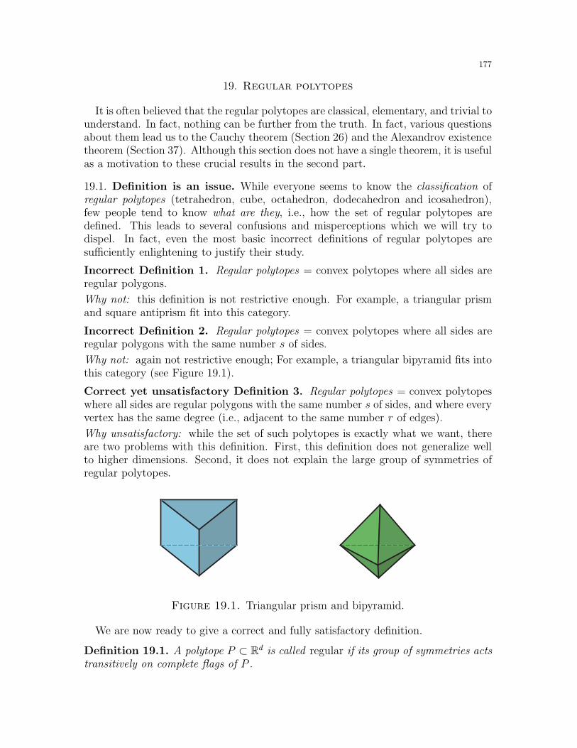
177

19. Regular polytopes

It is often believed that the regular polytopes are classical, elementary, and trivial tounderstand. In fact, nothing can be further from the truth. In fact, various questionsabout them lead us to the Cauchy theorem (Section 26) and the Alexandrov existencetheorem (Section 37). Although this section does not have a single theorem, it is usefulas a motivation to these crucial results in the second part.

19.1. Definition is an issue. While everyone seems to know the classification ofregular polytopes (tetrahedron, cube, octahedron, dodecahedron and icosahedron),few people tend to know what are they, i.e., how the set of regular polytopes aredefined. This leads to several confusions and misperceptions which we will try todispel. In fact, even the most basic incorrect definitions of regular polytopes aresufficiently enlightening to justify their study.

Incorrect Definition 1. Regular polytopes = convex polytopes where all sides areregular polygons.

Why not: this definition is not restrictive enough. For example, a triangular prismand square antiprism fit into this category.

Incorrect Definition 2. Regular polytopes = convex polytopes where all sides areregular polygons with the same number s of sides.

Why not: again not restrictive enough; For example, a triangular bipyramid fits intothis category (see Figure 19.1).

Correct yet unsatisfactory Definition 3. Regular polytopes = convex polytopeswhere all sides are regular polygons with the same number s of sides, and where everyvertex has the same degree (i.e., adjacent to the same number r of edges).

Why unsatisfactory: while the set of such polytopes is exactly what we want, thereare two problems with this definition. First, this definition does not generalize wellto higher dimensions. Second, it does not explain the large group of symmetries ofregular polytopes.

Figure 19.1. Triangular prism and bipyramid.

We are now ready to give a correct and fully satisfactory definition.

Definition 19.1. A polytope P ⊂ Rd is called regular if its group of symmetries actstransitively on complete flags of P .

178

Here by complete flags we mean a sequence: vertex ⊂ edge ⊂ 2-dimensional face⊂ . . . ⊂ P . Now consider the numerical consequences of the definition when d = 3.

Denote by Γ the group of symmetries of P . Let AF be the set of edges containedin face F . Since Γ acts transitively on complete flags, polytope P is face-transitive.Thus, |AF | = |AF ′|, for all faces F and F ′. In other words, all faces are polygonswith the same number s of sides.

Similarly, denote by Ev the set of edges containing vertex v of the polytope P .Again, by transitivity of the action of Γ we conclude that P is vertex-transitive.Thus, |Ev| = |Ev′ |, for all vertices v and v′. In other words, all vertices are adjacentto the same number r of edges. This gives the conditions in “definition 3”. Notethat P must also be edge-transitive, restricting the possibilities even further.

19.2. Classification of regular polytopes in R3. Let P ⊂ R3 be a regular convexpolytope, where the sides are regular s-gons, and all vertices are adjacent to r edges.Denote by n = |V | the number of vertices, m = |E| the number of edges, and f = |F|the number of faces. Counting all edges via vertices and faces we obtain:

2 ·m = n · r = f · s .Writing n and f through m, we rewrite Euler’s formula n−m+ f = 2 as follows:

2m

r− m +

2m

s= 2 ,

and finally1

r+

1

s=

1

m+

1

2.

From here either 1/r or 1/s is > 1/4, and since r, s,m ≥ 3, we can check all cases toconclude that

(r, s) ∈ (3, 3), (3, 4), (4, 3), (3, 5), (5, 3).These five cases correspond to the five platonic solids in the same order as listed inthe beginning of the previous subsection. It would seem that we are finished, exceptfor one annoying little problem:

How do we know these regular polytopes actually exist?

We discuss this “little problem” at length and eventually resolve it completely in thenext subsection.

19.3. Constructing polytopes is harder than you think. Well, we all know thatthese polytopes exist. Having seen them all over the place it is easy to take things forgranted. Of course, there must be a theoretical reason. After all, that was a crownachievement of Euclid. But are you really sure? Let us go over the list to see what isreally going on.

Naturally, there is little doubt the regular tetrahedron and the cube exist. Thecenters of faces of a cube give vertices of an octahedron. Same for the dodecahedron:it is formed by taking centers of faces of the icosahedron. Now, when we get toicosahedron we are in trouble. A priori, there is no theoretical reason why it shouldexist. Can we explicitly construct it?

179

(i) Coordinate approach. The icosahedron can be constructed by coordinates of all 12

vertices: (0,±1,±φ), (±1,±φ, 0), and (±φ, 0,±1), where φ = 1+√

52

is the golden ratio(see [Hada, §564]). It takes some minor checking to see that the convex hull of thesepoints forms an icosahedron. First, observe that the vertices lie on a sphere centeredat the origin, and thus in convex position. Cyclically permuting coordinates andchanging signs defines an action of the group Z3⋉Z

32 (of order 24) on all 120 = 12·5·2

complete flags. With one additional rotation around a diagonal (see Exercise 19.1),one can obtain the full group of symmetries Γ ≃ A5 × Z2 of order 120, and proveexistence of the icosahedron.

It is important to observe that the above argument was indirect: we did not reallyconstruct the icosahedron – we just checked someone else’s construction. Also, Euclidclearly could not have conceived this construction. So here is another approach.

(ii) Continuity argument. Start with a regular pentagon Q with side 1 and a penta-gon Q′ obtained from Q by rotation (see Figure 19.2). Start lifting Q up until at somepoint the side edges connecting two levels become equal to 1. This will happen bycontinuity. Finally, add a regular pentagonal cap on top and on the bottom to obtainan icosahedron (see Figure 19.2). Although, by construction, all faces are equilateraltriangles, this does not immediately imply that the resulting polytope is regular.

Now, consider the group of symmetries of the resulting polytope P . Clearly, we haveall symmetries which preserve the main diagonal (North to South Pole). This givesa group of symmetries with 20 elements. However, the action of the full symmetrygroup on vertices is not obviously transitive: to prove that P has all 120 symmetrieswe need to exhibit an orthogonal transformation which maps the main diagonal intoanother diagonals.

Q

Q′

Figure 19.2. Construction of the regular icosahedron, step by step.

(iii) Inscribing into a cube. Here is another approach, arguably more elegant. Drawintervals of length x symmetrically on each face of the square as in Figure 19.3. Denoteby Px a convex hull of these intervals. Beginning with a small length x, increase xuntil all edges of Px have the same length. Again, the resulting polytope P has allfaces equilateral triangles, but that in itself does not a priori prove that P is regular.

By construction, the group of symmetries of P is transitive on all vertices. Infact, already the subgroup of joint symmetries of P and the cube is transitive onthe vertices of P and has order 24. However, the action on faces is not obviously

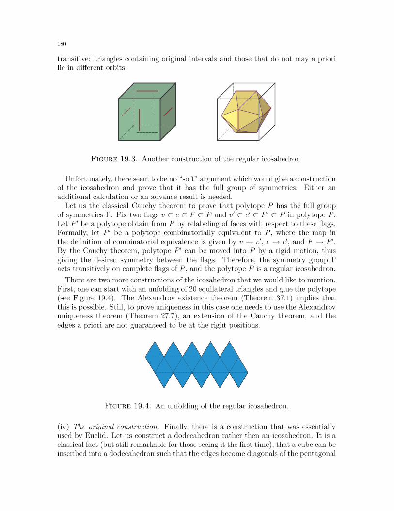
180

transitive: triangles containing original intervals and those that do not may a priorilie in different orbits.

Figure 19.3. Another construction of the regular icosahedron.

Unfortunately, there seem to be no “soft” argument which would give a constructionof the icosahedron and prove that it has the full group of symmetries. Either anadditional calculation or an advance result is needed.

Let us the classical Cauchy theorem to prove that polytope P has the full groupof symmetries Γ. Fix two flags v ⊂ e ⊂ F ⊂ P and v′ ⊂ e′ ⊂ F ′ ⊂ P in polytope P .Let P ′ be a polytope obtain from P by relabeling of faces with respect to these flags.Formally, let P ′ be a polytope combinatorially equivalent to P , where the map inthe definition of combinatorial equivalence is given by v → v′, e → e′, and F → F ′.By the Cauchy theorem, polytope P ′ can be moved into P by a rigid motion, thusgiving the desired symmetry between the flags. Therefore, the symmetry group Γacts transitively on complete flags of P , and the polytope P is a regular icosahedron.

There are two more constructions of the icosahedron that we would like to mention.First, one can start with an unfolding of 20 equilateral triangles and glue the polytope(see Figure 19.4). The Alexandrov existence theorem (Theorem 37.1) implies thatthis is possible. Still, to prove uniqueness in this case one needs to use the Alexandrovuniqueness theorem (Theorem 27.7), an extension of the Cauchy theorem, and theedges a priori are not guaranteed to be at the right positions.

Figure 19.4. An unfolding of the regular icosahedron.

(iv) The original construction. Finally, there is a construction that was essentiallyused by Euclid. Let us construct a dodecahedron rather then an icosahedron. It is aclassical fact (but still remarkable for those seeing it the first time), that a cube can beinscribed into a dodecahedron such that the edges become diagonals of the pentagonal

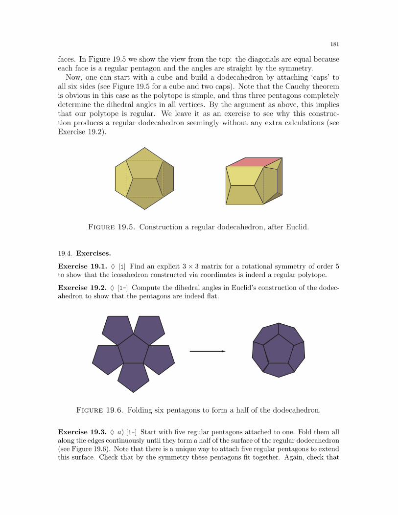
181

faces. In Figure 19.5 we show the view from the top: the diagonals are equal becauseeach face is a regular pentagon and the angles are straight by the symmetry.

Now, one can start with a cube and build a dodecahedron by attaching ‘caps’ toall six sides (see Figure 19.5 for a cube and two caps). Note that the Cauchy theoremis obvious in this case as the polytope is simple, and thus three pentagons completelydetermine the dihedral angles in all vertices. By the argument as above, this impliesthat our polytope is regular. We leave it as an exercise to see why this construc-tion produces a regular dodecahedron seemingly without any extra calculations (seeExercise 19.2).

Figure 19.5. Construction a regular dodecahedron, after Euclid.

19.4. Exercises.

Exercise 19.1. ♦ [1] Find an explicit 3 × 3 matrix for a rotational symmetry of order 5to show that the icosahedron constructed via coordinates is indeed a regular polytope.

Exercise 19.2. ♦ [1-] Compute the dihedral angles in Euclid’s construction of the dodec-ahedron to show that the pentagons are indeed flat.

Figure 19.6. Folding six pentagons to form a half of the dodecahedron.

Exercise 19.3. ♦ a) [1-] Start with five regular pentagons attached to one. Fold them allalong the edges continuously until they form a half of the surface of the regular dodecahedron(see Figure 19.6). Note that there is a unique way to attach five regular pentagons to extendthis surface. Check that by the symmetry these pentagons fit together. Again, check that

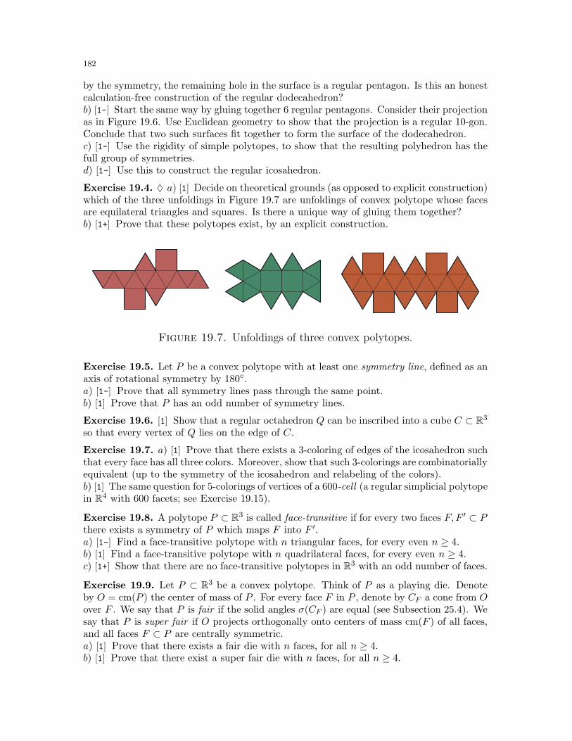
182

by the symmetry, the remaining hole in the surface is a regular pentagon. Is this an honestcalculation-free construction of the regular dodecahedron?b) [1-] Start the same way by gluing together 6 regular pentagons. Consider their projectionas in Figure 19.6. Use Euclidean geometry to show that the projection is a regular 10-gon.Conclude that two such surfaces fit together to form the surface of the dodecahedron.c) [1-] Use the rigidity of simple polytopes, to show that the resulting polyhedron has thefull group of symmetries.d) [1-] Use this to construct the regular icosahedron.

Exercise 19.4. ♦ a) [1] Decide on theoretical grounds (as opposed to explicit construction)which of the three unfoldings in Figure 19.7 are unfoldings of convex polytope whose facesare equilateral triangles and squares. Is there a unique way of gluing them together?b) [1+] Prove that these polytopes exist, by an explicit construction.

Figure 19.7. Unfoldings of three convex polytopes.

Exercise 19.5. Let P be a convex polytope with at least one symmetry line, defined as anaxis of rotational symmetry by 180.a) [1-] Prove that all symmetry lines pass through the same point.b) [1] Prove that P has an odd number of symmetry lines.

Exercise 19.6. [1] Show that a regular octahedron Q can be inscribed into a cube C ⊂ R3

so that every vertex of Q lies on the edge of C.

Exercise 19.7. a) [1] Prove that there exists a 3-coloring of edges of the icosahedron suchthat every face has all three colors. Moreover, show that such 3-colorings are combinatoriallyequivalent (up to the symmetry of the icosahedron and relabeling of the colors).b) [1] The same question for 5-colorings of vertices of a 600-cell (a regular simplicial polytopein R4 with 600 facets; see Exercise 19.15).

Exercise 19.8. A polytope P ⊂ R3 is called face-transitive if for every two faces F,F ′ ⊂ Pthere exists a symmetry of P which maps F into F ′.a) [1-] Find a face-transitive polytope with n triangular faces, for every even n ≥ 4.b) [1] Find a face-transitive polytope with n quadrilateral faces, for every even n ≥ 4.c) [1+] Show that there are no face-transitive polytopes in R3 with an odd number of faces.

Exercise 19.9. Let P ⊂ R3 be a convex polytope. Think of P as a playing die. Denoteby O = cm(P ) the center of mass of P . For every face F in P , denote by CF a cone from Oover F . We say that P is fair if the solid angles σ(CF ) are equal (see Subsection 25.4). Wesay that P is super fair if O projects orthogonally onto centers of mass cm(F ) of all faces,and all faces F ⊂ P are centrally symmetric.a) [1] Prove that there exists a fair die with n faces, for all n ≥ 4.b) [1] Prove that there exist a super fair die with n faces, for all n ≥ 4.

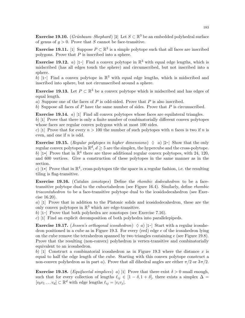
183

Exercise 19.10. (Grunbaum–Shephard) [2] Let S ⊂ R3 be an embedded polyhedral surfaceof genus of g > 0. Prove that S cannot be face-transitive.

Exercise 19.11. [1] Suppose P ⊂ R3 is a simple polytope such that all faces are inscribedpolygons. Prove that P is inscribed into a sphere.

Exercise 19.12. a) [1-] Find a convex polytope in R3 with equal edge lengths, which ismidscribed (has all edges touch the sphere) and circumscribed, but not inscribed into asphere.b) [1-] Find a convex polytope in R3 with equal edge lengths, which is midscribed andinscribed into sphere, but not circumscribed around a sphere.

Exercise 19.13. Let P ⊂ R3 be a convex polytope which is midscribed and has edges ofequal length.a) Suppose one of the faces of P is odd-sided. Prove that P is also inscribed.b) Suppose all faces of P have the same number of sides. Prove that P is circumscribed.

Exercise 19.14. a) [1] Find all convex polytopes whose faces are equilateral triangles.b) [1] Prove that there is only a finite number of combinatorially different convex polytopeswhose faces are regular convex polygons with at most 100 sides.c) [1] Prove that for every n > 100 the number of such polytopes with n faces is two if n iseven, and one if n is odd.

Exercise 19.15. (Regular polytopes in higher dimensions) ♦ a) [2-] Show that the onlyregular convex polytopes in Rd, d ≥ 5 are the simplex, the hypercube and the cross-polytope.b) [1+] Prove that in R4 there are three additional regular convex polytopes, with 24, 120,and 600 vertices. Give a construction of these polytopes in the same manner as in thesection.c) [1+] Prove that in R4, cross-polytopes tile the space in a regular fashion, i.e. the resultingtiling is flag-transitive.

Exercise 19.16. (Catalan zonotopes) Define the rhombic dodecahedron to be a face-transitive polytope dual to the cuboctahedron (see Figure 16.4). Similarly, define rhombictriacontahedron to be a face-transitive polytope dual to the icosidodecahedron (see Exer-cise 16.20).a) [1] Prove that in addition to the Platonic solids and icosidodecahedron, these are theonly convex polytopes in R3 which are edge-transitive.b) [1-] Prove that both polyhedra are zonotopes (see Exercise 7.16).c) [1] Find an explicit decomposition of both polyhedra into parallelepipeds.

Exercise 19.17. (Jessen’s orthogonal icosahedron) ♦ a) [1-] Start with a regular icosahe-dron positioned in a cube as in Figure 19.3. For every (red) edge e of the icosahedron lyingon the cube remove the tetrahedron spanned by two triangles containing e (see Figure 19.8).Prove that the resulting (non-convex) polyhedron is vertex-transitive and combinatoriallyequivalent to an icosahedron.b) [1] Construct a combinatorial icosahedron as in Figure 19.3 where the distance x isequal to half the edge length of the cube. Starting with this convex polytope construct anon-convex polyhedron as in part a). Prove that all dihedral angles are either π/2 or 3π/2.

Exercise 19.18. (Equifacetal simplices) a) [1] Prove that there exist δ > 0 small enough,such that for every collection of lengths ℓij ∈ [1 − δ, 1 + δ], there exists a simplex ∆ =[v0v1 . . . vd] ⊂ Rd with edge lengths ℓij = |vivj |.

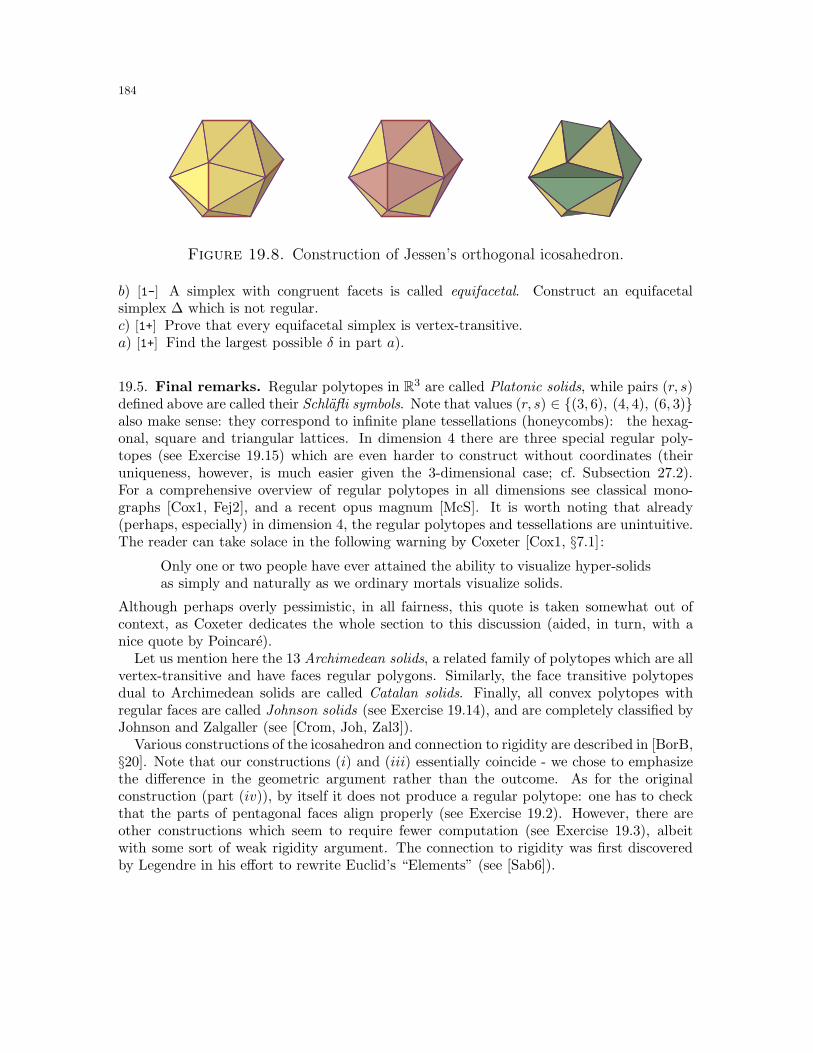
184

Figure 19.8. Construction of Jessen’s orthogonal icosahedron.

b) [1-] A simplex with congruent facets is called equifacetal. Construct an equifacetalsimplex ∆ which is not regular.c) [1+] Prove that every equifacetal simplex is vertex-transitive.a) [1+] Find the largest possible δ in part a).

19.5. Final remarks. Regular polytopes in R3 are called Platonic solids, while pairs (r, s)defined above are called their Schlafli symbols. Note that values (r, s) ∈ (3, 6), (4, 4), (6, 3)also make sense: they correspond to infinite plane tessellations (honeycombs): the hexag-onal, square and triangular lattices. In dimension 4 there are three special regular poly-topes (see Exercise 19.15) which are even harder to construct without coordinates (theiruniqueness, however, is much easier given the 3-dimensional case; cf. Subsection 27.2).For a comprehensive overview of regular polytopes in all dimensions see classical mono-graphs [Cox1, Fej2], and a recent opus magnum [McS]. It is worth noting that already(perhaps, especially) in dimension 4, the regular polytopes and tessellations are unintuitive.The reader can take solace in the following warning by Coxeter [Cox1, §7.1]:

Only one or two people have ever attained the ability to visualize hyper-solidsas simply and naturally as we ordinary mortals visualize solids.

Although perhaps overly pessimistic, in all fairness, this quote is taken somewhat out ofcontext, as Coxeter dedicates the whole section to this discussion (aided, in turn, with anice quote by Poincare).

Let us mention here the 13 Archimedean solids, a related family of polytopes which are allvertex-transitive and have faces regular polygons. Similarly, the face transitive polytopesdual to Archimedean solids are called Catalan solids. Finally, all convex polytopes withregular faces are called Johnson solids (see Exercise 19.14), and are completely classified byJohnson and Zalgaller (see [Crom, Joh, Zal3]).

Various constructions of the icosahedron and connection to rigidity are described in [BorB,§20]. Note that our constructions (i) and (iii) essentially coincide - we chose to emphasizethe difference in the geometric argument rather than the outcome. As for the originalconstruction (part (iv)), by itself it does not produce a regular polytope: one has to checkthat the parts of pentagonal faces align properly (see Exercise 19.2). However, there areother constructions which seem to require fewer computation (see Exercise 19.3), albeitwith some sort of weak rigidity argument. The connection to rigidity was first discoveredby Legendre in his effort to rewrite Euclid’s “Elements” (see [Sab6]).

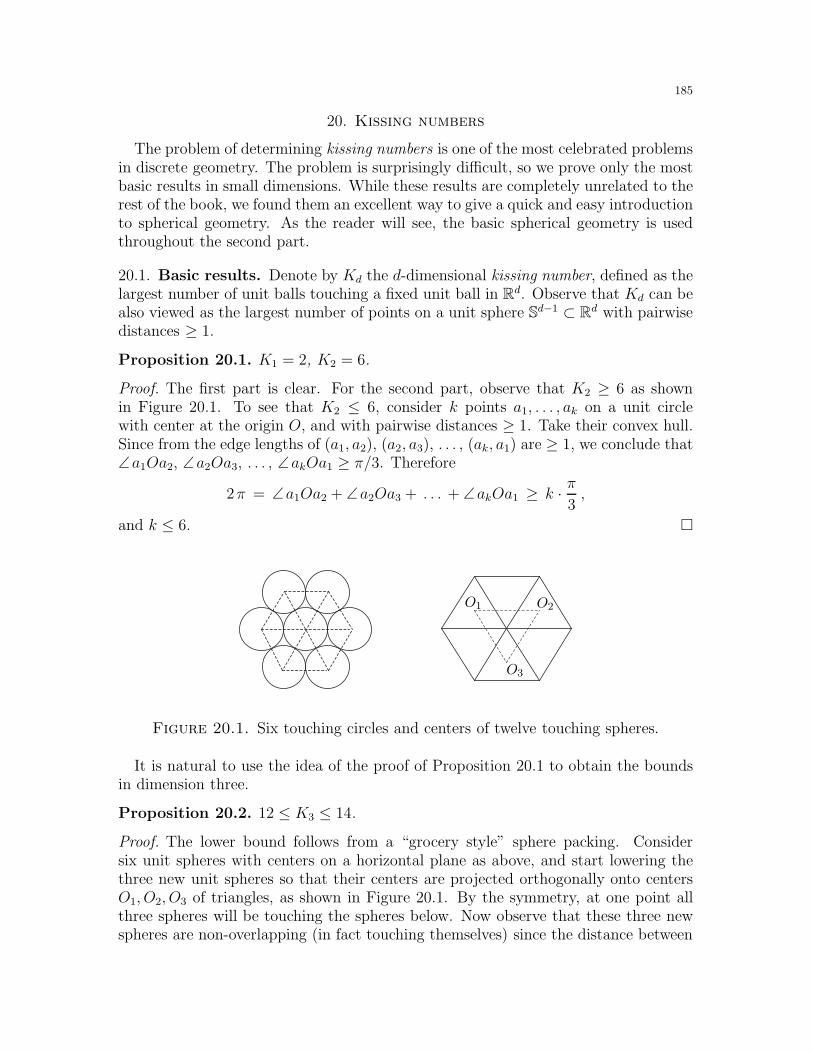
185

20. Kissing numbers

The problem of determining kissing numbers is one of the most celebrated problemsin discrete geometry. The problem is surprisingly difficult, so we prove only the mostbasic results in small dimensions. While these results are completely unrelated to therest of the book, we found them an excellent way to give a quick and easy introductionto spherical geometry. As the reader will see, the basic spherical geometry is usedthroughout the second part.

20.1. Basic results. Denote by Kd the d-dimensional kissing number, defined as thelargest number of unit balls touching a fixed unit ball in Rd. Observe that Kd can bealso viewed as the largest number of points on a unit sphere Sd−1 ⊂ Rd with pairwisedistances ≥ 1.

Proposition 20.1. K1 = 2, K2 = 6.

Proof. The first part is clear. For the second part, observe that K2 ≥ 6 as shownin Figure 20.1. To see that K2 ≤ 6, consider k points a1, . . . , ak on a unit circlewith center at the origin O, and with pairwise distances ≥ 1. Take their convex hull.Since from the edge lengths of (a1, a2), (a2, a3), . . . , (ak, a1) are ≥ 1, we conclude that∠a1Oa2, ∠a2Oa3, . . . , ∠akOa1 ≥ π/3. Therefore

2π = ∠a1Oa2 + ∠a2Oa3 + . . . + ∠akOa1 ≥ k · π3,

and k ≤ 6.

O1 O2

O3

Figure 20.1. Six touching circles and centers of twelve touching spheres.

It is natural to use the idea of the proof of Proposition 20.1 to obtain the boundsin dimension three.

Proposition 20.2. 12 ≤ K3 ≤ 14.

Proof. The lower bound follows from a “grocery style” sphere packing. Considersix unit spheres with centers on a horizontal plane as above, and start lowering thethree new unit spheres so that their centers are projected orthogonally onto centersO1, O2, O3 of triangles, as shown in Figure 20.1. By the symmetry, at one point allthree spheres will be touching the spheres below. Now observe that these three newspheres are non-overlapping (in fact touching themselves) since the distance between

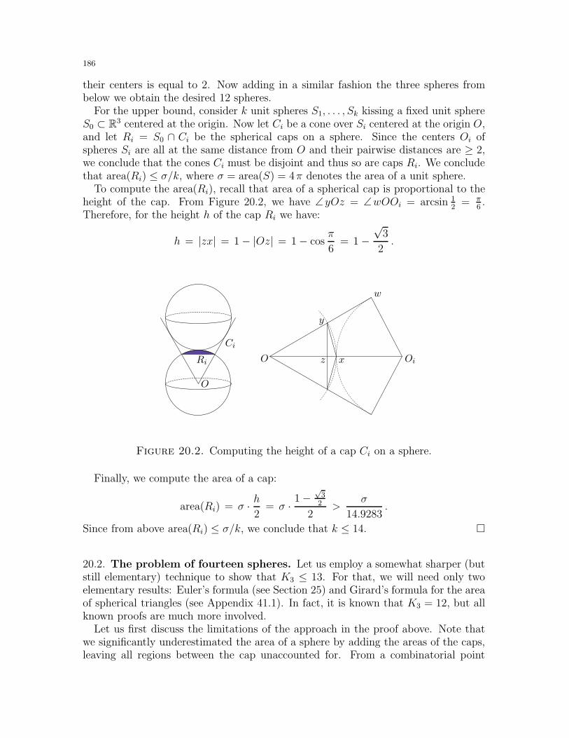
186

their centers is equal to 2. Now adding in a similar fashion the three spheres frombelow we obtain the desired 12 spheres.

For the upper bound, consider k unit spheres S1, . . . , Sk kissing a fixed unit sphereS0 ⊂ R3 centered at the origin. Now let Ci be a cone over Si centered at the origin O,and let Ri = S0 ∩ Ci be the spherical caps on a sphere. Since the centers Oi ofspheres Si are all at the same distance from O and their pairwise distances are ≥ 2,we conclude that the cones Ci must be disjoint and thus so are caps Ri. We concludethat area(Ri) ≤ σ/k, where σ = area(S) = 4π denotes the area of a unit sphere.

To compute the area(Ri), recall that area of a spherical cap is proportional to theheight of the cap. From Figure 20.2, we have ∠yOz = ∠wOOi = arcsin 1

2= π

6.

Therefore, for the height h of the cap Ri we have:

h = |zx| = 1− |Oz| = 1− cosπ

6= 1−

√3

2.

Ci

Ri x

y

z

w

O

O Oi

Figure 20.2. Computing the height of a cap Ci on a sphere.

Finally, we compute the area of a cap:

area(Ri) = σ · h2

= σ · 1−√

32

2>

σ

14.9283.

Since from above area(Ri) ≤ σ/k, we conclude that k ≤ 14.

20.2. The problem of fourteen spheres. Let us employ a somewhat sharper (butstill elementary) technique to show that K3 ≤ 13. For that, we will need only twoelementary results: Euler’s formula (see Section 25) and Girard’s formula for the areaof spherical triangles (see Appendix 41.1). In fact, it is known that K3 = 12, but allknown proofs are much more involved.

Let us first discuss the limitations of the approach in the proof above. Note thatwe significantly underestimated the area of a sphere by adding the areas of the caps,leaving all regions between the cap unaccounted for. From a combinatorial point

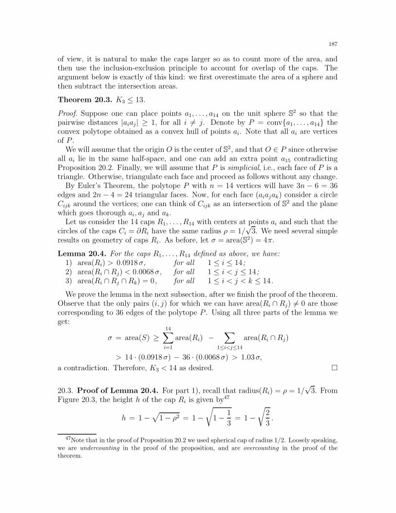
187

of view, it is natural to make the caps larger so as to count more of the area, andthen use the inclusion-exclusion principle to account for overlap of the caps. Theargument below is exactly of this kind: we first overestimate the area of a sphere andthen subtract the intersection areas.

Theorem 20.3. K3 ≤ 13.

Proof. Suppose one can place points a1, . . . , a14 on the unit sphere S2 so that thepairwise distances |aiaj | ≥ 1, for all i 6= j. Denote by P = conva1, . . . , a14 theconvex polytope obtained as a convex hull of points ai. Note that all ai are verticesof P .

We will assume that the origin O is the center of S2, and that O ∈ P since otherwiseall ai lie in the same half-space, and one can add an extra point a15 contradictingProposition 20.2. Finally, we will assume that P is simplicial, i.e., each face of P is atriangle. Otherwise, triangulate each face and proceed as follows without any change.

By Euler’s Theorem, the polytope P with n = 14 vertices will have 3n − 6 = 36edges and 2n− 4 = 24 triangular faces. Now, for each face (aiajak) consider a circleCijk around the vertices; one can think of Cijk as an intersection of S2 and the planewhich goes thorough ai, aj and ak.

Let us consider the 14 caps R1, . . . , R14 with centers at points ai and such that thecircles of the caps Ci = ∂Ri have the same radius ρ = 1/

√3. We need several simple

results on geometry of caps Ri. As before, let σ = area(S2) = 4π.

Lemma 20.4. For the caps R1, . . . , R14 defined as above, we have:1) area(Ri) > 0.0918σ, for all 1 ≤ i ≤ 14;2) area(Ri ∩Rj) < 0.0068σ, for all 1 ≤ i < j ≤ 14;3) area(Ri ∩Rj ∩ Rk) = 0, for all 1 ≤ i < j < k ≤ 14.

We prove the lemma in the next subsection, after we finish the proof of the theorem.Observe that the only pairs (i, j) for which we can have area(Ri ∩ Rj) 6= 0 are thosecorresponding to 36 edges of the polytope P . Using all three parts of the lemma weget:

σ = area(S) ≥14∑

i=1

area(Ri) −∑

1≤i<j≤14

area(Ri ∩Rj)

> 14 · (0.0918σ) − 36 · (0.0068σ) > 1.03σ,

a contradiction. Therefore, K3 < 14 as desired.

20.3. Proof of Lemma 20.4. For part 1), recall that radius(Ri) = ρ = 1/√

3. FromFigure 20.3, the height h of the cap Ri is given by47

h = 1−√

1− ρ2 = 1−√

1− 1

3= 1−

√2

3.

47Note that in the proof of Proposition 20.2 we used spherical cap of radius 1/2. Loosely speaking,we are undercounting in the proof of the proposition, and are overcounting in the proof of thetheorem.

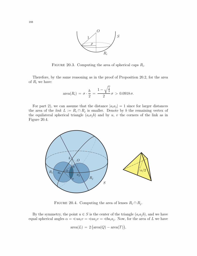
188

S

O

1

ρ

Ri

Figure 20.3. Computing the area of spherical caps Ri.

Therefore, by the same reasoning as in the proof of Proposition 20.2, for the areaof Ri we have:

area(Ri) = σ · h2

=1−

√23

2σ > 0.0918σ.

For part 2), we can assume that the distance |aiaj | = 1 since for larger distancesthe area of the link L := Ri ∩ Rj is smaller. Denote by b the remaining vertex ofthe equilateral spherical triangle (aiajb) and by u, v the corners of the link as inFigure 20.4.

S

Ri

Rj

O

ai aj

b

u

v

α α/2

Figure 20.4. Computing the area of lenses Ri ∩ Rj.

By the symmetry, the point u ∈ S is the center of the triangle (aiajb), and we haveequal spherical angles α = ∢uaiv = ∢uajv = ∢baiaj . Now, for the area of L we have

area(L) = 2(area(Q)− area(T )

),

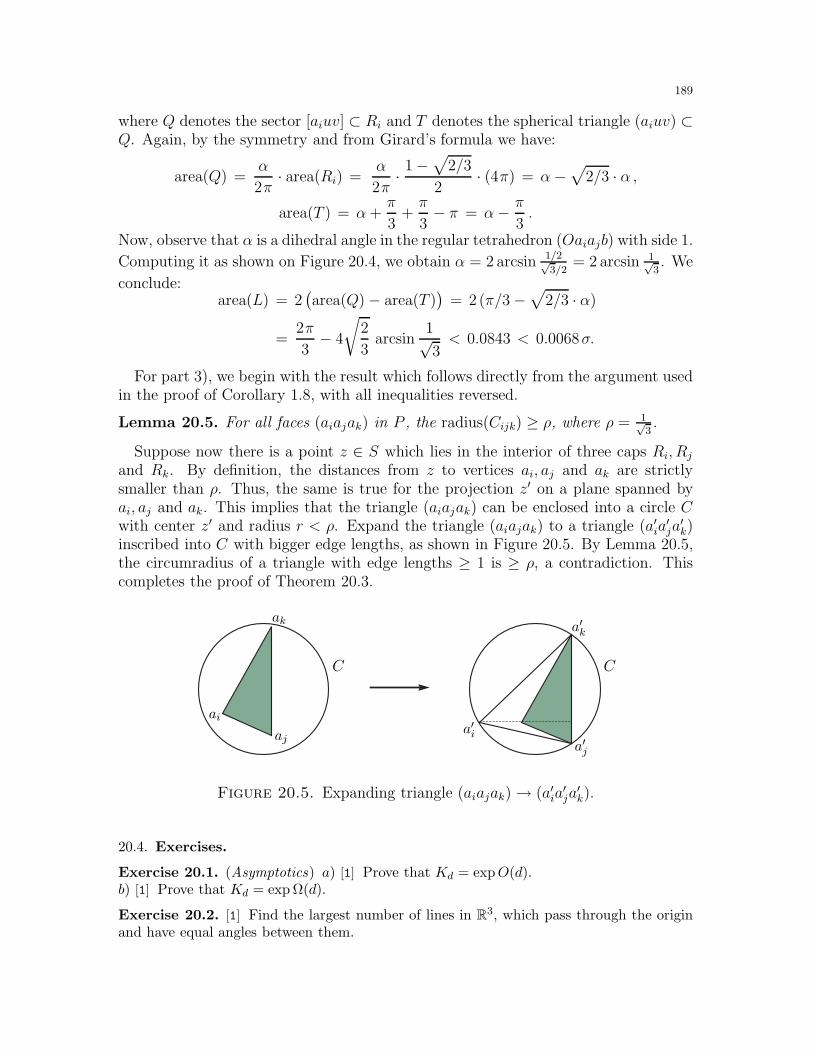
189

where Q denotes the sector [aiuv] ⊂ Ri and T denotes the spherical triangle (aiuv) ⊂Q. Again, by the symmetry and from Girard’s formula we have:

area(Q) =α

2π· area(Ri) =

α

2π· 1−

√2/3

2· (4π) = α−

√2/3 · α ,

area(T ) = α+π

3+π

3− π = α− π

3.

Now, observe that α is a dihedral angle in the regular tetrahedron (Oaiajb) with side 1.

Computing it as shown on Figure 20.4, we obtain α = 2 arcsin 1/2√3/2

= 2 arcsin 1√3. We

conclude:area(L) = 2

(area(Q)− area(T )

)= 2(π/3−

√2/3 · α)

=2π

3− 4

√2

3arcsin

1√3< 0.0843 < 0.0068σ.

For part 3), we begin with the result which follows directly from the argument usedin the proof of Corollary 1.8, with all inequalities reversed.

Lemma 20.5. For all faces (aiajak) in P , the radius(Cijk) ≥ ρ, where ρ = 1√3.

Suppose now there is a point z ∈ S which lies in the interior of three caps Ri, Rj

and Rk. By definition, the distances from z to vertices ai, aj and ak are strictlysmaller than ρ. Thus, the same is true for the projection z′ on a plane spanned byai, aj and ak. This implies that the triangle (aiajak) can be enclosed into a circle Cwith center z′ and radius r < ρ. Expand the triangle (aiajak) to a triangle (a′ia

′ja

′k)

inscribed into C with bigger edge lengths, as shown in Figure 20.5. By Lemma 20.5,the circumradius of a triangle with edge lengths ≥ 1 is ≥ ρ, a contradiction. Thiscompletes the proof of Theorem 20.3.

CC

ai

aj

ak

a′ia′j

a′k

Figure 20.5. Expanding triangle (aiajak)→ (a′ia′ja

′k).

20.4. Exercises.

Exercise 20.1. (Asymptotics) a) [1] Prove that Kd = expO(d).b) [1] Prove that Kd = exp Ω(d).

Exercise 20.2. [1] Find the largest number of lines in R3, which pass through the originand have equal angles between them.

190

Exercise 20.3. [1+] Let P ⊂ R3 be a convex polytope with 19 faces. Suppose P iscircumscribed around a sphere of radius 10. Prove that diam(P ) > 21.

Exercise 20.4. [1] Let x1, . . . , x30 ∈ S2 be points on a unit sphere. Prove that there exist1 ≤ i < j ≤ 30, such that ∣∣xixj

∣∣S2 <

π

4.

In other words, show that some two of the vectors−−→Oxi have angle < π/4 between them.

Exercise 20.5. a) [1] Suppose n points on a unit sphere have pairwise spherical distances≥ π/2. Prove that n ≤ 6, and that for n = 6 these points must be vertices of an inscribedregular octahedron.b) [1+] Prove an icosahedral analogue of a).c) [2-] Suppose x1, . . . , xn and y1, . . . , yn are two configurations of points in the unitsphere S2, such that |xixj | ≥ |yiyj| for all i, j ∈ [n]. Suppose further thatO ∈ convx1, . . . , xn,where O is the center of S2. Prove that |xixj| = |yiyj| for all i, j ∈ [n].

Exercise 20.6. a) [1-] Is it possible to cover the plane by a union of parabolas, i.e., regionsobtain by translations and rotations of y ≥ ax2, where a > 0.b) [1] Suppose in the space R3 there is a finite number of disjoint cones, i.e., regions obtainby translations and rotations of x2 + y2 ≤ az, where a > 0. Prove that these cones cannotbe moved to cover the whole space.

Exercise 20.7. On a unit sphere, define an α-arc to be an arc of a great circle of length α.a) [1-] For every α < π, prove that there are infinitely many not self-intersecting α-arcs ona unit sphere.b) [1] For α = 5/3π, prove that there are at most two not self-intersecting α-arcs on a unitsphere.c) [1] Prove that there is an unbounded number of not self-intersecting π-arcs on a unitsphere.d) [1+] For every α > π, prove that there is at most a bounded number n = n(α) of notself-intersecting α-arcs on a unit sphere.

Exercise 20.8. Prove that the following triangles (given by their angles) can tile thesphere S2 without overlap:a) [1-] (90, 90, 1), (90, 60, 60), (120, 60, 60),b) [1] (120, 45, 45), (72, 60, 60), (150, 60, 60),c) [1+] (80, 60, 60), (100, 60, 60), (100, 80, 60).

Exercise 20.9. ♦ a) [1-] Place the centers of twelve unit spheres in R3 at the verticesof the icosahedron inscribed into a sphere of radius 2. Check that these spheres are notoverlapping and, moreover, no two of them touch each other. This gives an alternativeproof of the lower bound in Proposition 20.2.b) [2-] In a), the outside spheres can be continuously moved while they remain non-overlapping and touching the center sphere. Is it possible to switch any two spheres thatway?c) [2+] Can these twelve spheres be moved into twelve spheres in the “grocery style” spherearrangement?

Exercise 20.10. Denote by KCd the number of infinite cylinders of unit radius in Rd,which are non-overlapping and touching the unit sphere. Such configuration is called kissingcylinders.

191

a) [1-] Prove that KCd ≥ Kd−1.b) [1-] Find a continuous family of different configurations of six kissing cylinders in R3

(different up to rotations).c) [2-] Prove that KC3 ≤ 7.d) [∗] Prove that KC3 ≤ 6.

Exercise 20.11. For a finite arrangement B of balls in Rd with disjoint interior (notnecessarily of the same radii), denote by a(B) their average kissing number. Define AKd tobe the supremum of a(B) over all finite ball arrangements.a) [1-] Show that the AKd > a(B) for any finite B.b) [1] Prove that AK3 > 12.c) [1] Prove that AKd ≤ 2Kd.

d) [2] Prove that AK3 ≤ 8 + 4√

3.

Exercise 20.12. (Pairwise kissing spheres) Denote by PKd the maximal number of pair-wise kissing spheres in Rd (possibly, of different radius).a) [1-] Use the previous exercise to show that PKd = expO(n). Explain the difference withExercise 42.45.b) [1] Use the algebraic approach (see Section 31) to show that PKd = O(d).c) [1] Prove that PKd = d+ 2.

20.5. Final remarks. Finding kissing numbers Kd is a classical problem connected tothe study of error-correcting codes, lattices, number theory and many problems in geome-try [ConS, Fej2, Zon1] (see also [Bez] for a recent survey). Proving that K3 = 12 is known asthe Newton–Gregory problem named after their celebrated exchange in 1694. The problemwas resolved by Schutte and van der Waerden only in 1953, but most known proofs arequite technical. In fact, this section can be viewed as an introduction to Leech’s proof, anelementary presentation of which recently appeared in [Mae2].

We refer to [Mus6] for a recent interesting proof of K3 = 12. Let us also note that while

the exact value K4 = 24 was determined recently by Musin [Mus5], the kissing numbers

K8 = 240 and K24 = 196560 have been known since 1979 (see [ConS, Mus5, PfeZ]). The

proof of Theorem 20.3 presented in this section is a minor reworking of the proof in [Yag2].

192

Part II

Discrete Geometry of Curves and Surfaces

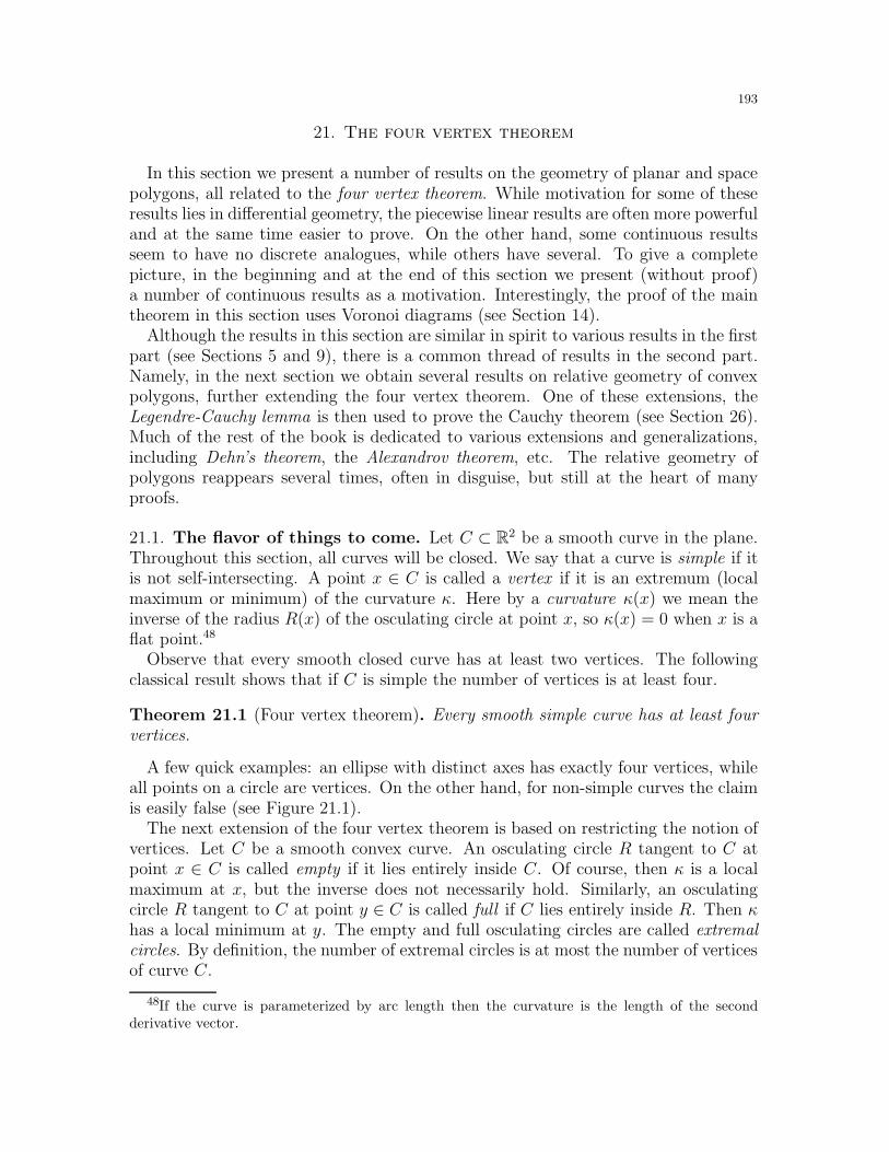
193

21. The four vertex theorem

In this section we present a number of results on the geometry of planar and spacepolygons, all related to the four vertex theorem. While motivation for some of theseresults lies in differential geometry, the piecewise linear results are often more powerfuland at the same time easier to prove. On the other hand, some continuous resultsseem to have no discrete analogues, while others have several. To give a completepicture, in the beginning and at the end of this section we present (without proof)a number of continuous results as a motivation. Interestingly, the proof of the maintheorem in this section uses Voronoi diagrams (see Section 14).

Although the results in this section are similar in spirit to various results in the firstpart (see Sections 5 and 9), there is a common thread of results in the second part.Namely, in the next section we obtain several results on relative geometry of convexpolygons, further extending the four vertex theorem. One of these extensions, theLegendre-Cauchy lemma is then used to prove the Cauchy theorem (see Section 26).Much of the rest of the book is dedicated to various extensions and generalizations,including Dehn’s theorem, the Alexandrov theorem, etc. The relative geometry ofpolygons reappears several times, often in disguise, but still at the heart of manyproofs.

21.1. The flavor of things to come. Let C ⊂ R2 be a smooth curve in the plane.Throughout this section, all curves will be closed. We say that a curve is simple if itis not self-intersecting. A point x ∈ C is called a vertex if it is an extremum (localmaximum or minimum) of the curvature κ. Here by a curvature κ(x) we mean theinverse of the radius R(x) of the osculating circle at point x, so κ(x) = 0 when x is aflat point.48

Observe that every smooth closed curve has at least two vertices. The followingclassical result shows that if C is simple the number of vertices is at least four.

Theorem 21.1 (Four vertex theorem). Every smooth simple curve has at least fourvertices.

A few quick examples: an ellipse with distinct axes has exactly four vertices, whileall points on a circle are vertices. On the other hand, for non-simple curves the claimis easily false (see Figure 21.1).

The next extension of the four vertex theorem is based on restricting the notion ofvertices. Let C be a smooth convex curve. An osculating circle R tangent to C atpoint x ∈ C is called empty if it lies entirely inside C. Of course, then κ is a localmaximum at x, but the inverse does not necessarily hold. Similarly, an osculatingcircle R tangent to C at point y ∈ C is called full if C lies entirely inside R. Then κhas a local minimum at y. The empty and full osculating circles are called extremalcircles. By definition, the number of extremal circles is at most the number of verticesof curve C.

48If the curve is parameterized by arc length then the curvature is the length of the secondderivative vector.

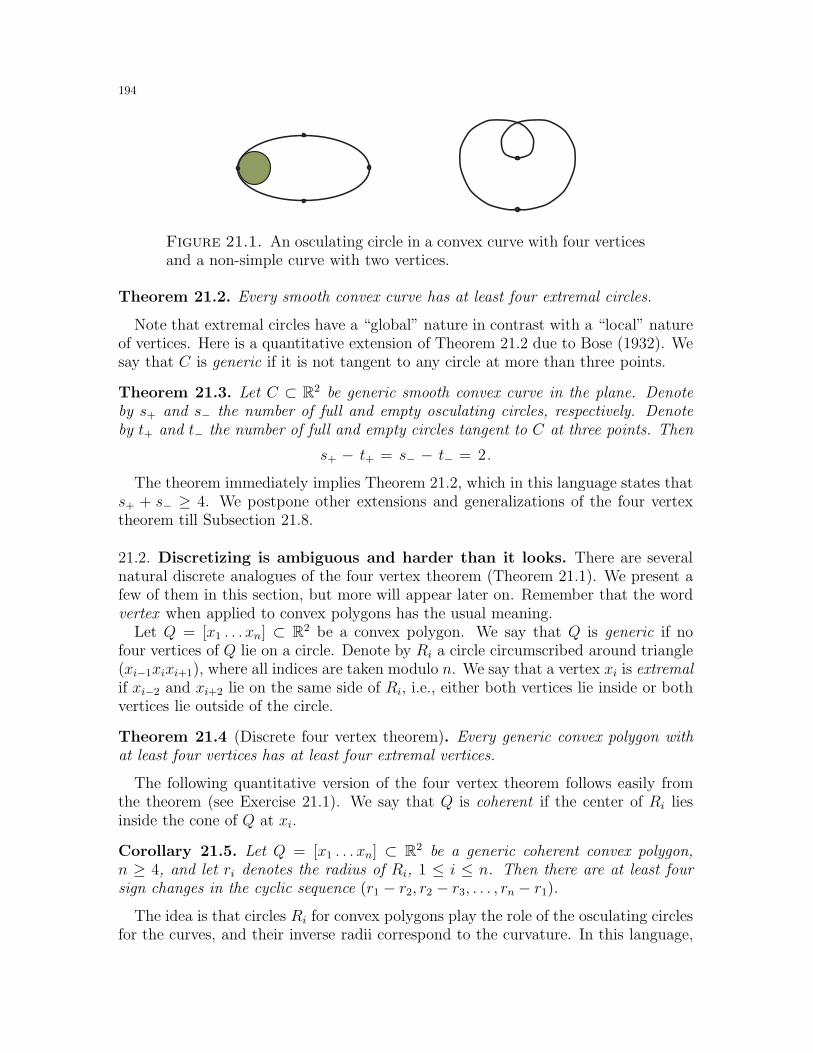
194

Figure 21.1. An osculating circle in a convex curve with four verticesand a non-simple curve with two vertices.

Theorem 21.2. Every smooth convex curve has at least four extremal circles.

Note that extremal circles have a “global” nature in contrast with a “local” natureof vertices. Here is a quantitative extension of Theorem 21.2 due to Bose (1932). Wesay that C is generic if it is not tangent to any circle at more than three points.

Theorem 21.3. Let C ⊂ R2 be generic smooth convex curve in the plane. Denoteby s+ and s− the number of full and empty osculating circles, respectively. Denoteby t+ and t− the number of full and empty circles tangent to C at three points. Then

s+ − t+ = s− − t− = 2.

The theorem immediately implies Theorem 21.2, which in this language states thats+ + s− ≥ 4. We postpone other extensions and generalizations of the four vertextheorem till Subsection 21.8.

21.2. Discretizing is ambiguous and harder than it looks. There are severalnatural discrete analogues of the four vertex theorem (Theorem 21.1). We present afew of them in this section, but more will appear later on. Remember that the wordvertex when applied to convex polygons has the usual meaning.

Let Q = [x1 . . . xn] ⊂ R2 be a convex polygon. We say that Q is generic if nofour vertices of Q lie on a circle. Denote by Ri a circle circumscribed around triangle(xi−1xixi+1), where all indices are taken modulo n. We say that a vertex xi is extremalif xi−2 and xi+2 lie on the same side of Ri, i.e., either both vertices lie inside or bothvertices lie outside of the circle.

Theorem 21.4 (Discrete four vertex theorem). Every generic convex polygon withat least four vertices has at least four extremal vertices.

The following quantitative version of the four vertex theorem follows easily fromthe theorem (see Exercise 21.1). We say that Q is coherent if the center of Ri liesinside the cone of Q at xi.

Corollary 21.5. Let Q = [x1 . . . xn] ⊂ R2 be a generic coherent convex polygon,n ≥ 4, and let ri denotes the radius of Ri, 1 ≤ i ≤ n. Then there are at least foursign changes in the cyclic sequence (r1 − r2, r2 − r3, . . . , rn − r1).

The idea is that circles Ri for convex polygons play the role of the osculating circlesfor the curves, and their inverse radii correspond to the curvature. In this language,

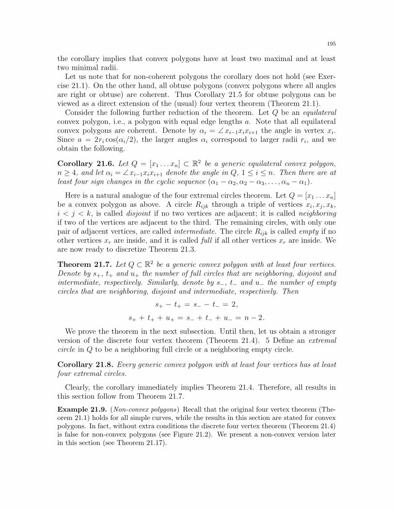
195

the corollary implies that convex polygons have at least two maximal and at leasttwo minimal radii.

Let us note that for non-coherent polygons the corollary does not hold (see Exer-cise 21.1). On the other hand, all obtuse polygons (convex polygons where all anglesare right or obtuse) are coherent. Thus Corollary 21.5 for obtuse polygons can beviewed as a direct extension of the (usual) four vertex theorem (Theorem 21.1).

Consider the following further reduction of the theorem. Let Q be an equilateralconvex polygon, i.e., a polygon with equal edge lengths a. Note that all equilateralconvex polygons are coherent. Denote by αi = ∠xi−1xixi+1 the angle in vertex xi.Since a = 2ri cos(αi/2), the larger angles αi correspond to larger radii ri, and weobtain the following.

Corollary 21.6. Let Q = [x1 . . . xn] ⊂ R2 be a generic equilateral convex polygon,n ≥ 4, and let αi = ∠xi−1xixi+1 denote the angle in Q, 1 ≤ i ≤ n. Then there are atleast four sign changes in the cyclic sequence (α1 − α2, α2 − α3, . . . , αn − α1).

Here is a natural analogue of the four extremal circles theorem. Let Q = [x1 . . . xn]be a convex polygon as above. A circle Rijk through a triple of vertices xi, xj , xk,i < j < k, is called disjoint if no two vertices are adjacent; it is called neighboringif two of the vertices are adjacent to the third. The remaining circles, with only onepair of adjacent vertices, are called intermediate. The circle Rijk is called empty if noother vertices xr are inside, and it is called full if all other vertices xr are inside. Weare now ready to discretize Theorem 21.3.

Theorem 21.7. Let Q ⊂ R2 be a generic convex polygon with at least four vertices.Denote by s+, t+ and u+ the number of full circles that are neighboring, disjoint andintermediate, respectively. Similarly, denote by s−, t− and u− the number of emptycircles that are neighboring, disjoint and intermediate, respectively. Then

s+ − t+ = s− − t− = 2,

s+ + t+ + u+ = s− + t− + u− = n− 2.

We prove the theorem in the next subsection. Until then, let us obtain a strongerversion of the discrete four vertex theorem (Theorem 21.4). 5 Define an extremalcircle in Q to be a neighboring full circle or a neighboring empty circle.

Corollary 21.8. Every generic convex polygon with at least four vertices has at leastfour extremal circles.

Clearly, the corollary immediately implies Theorem 21.4. Therefore, all results inthis section follow from Theorem 21.7.

Example 21.9. (Non-convex polygons) Recall that the original four vertex theorem (The-orem 21.1) holds for all simple curves, while the results in this section are stated for convexpolygons. In fact, without extra conditions the discrete four vertex theorem (Theorem 21.4)is false for non-convex polygons (see Figure 21.2). We present a non-convex version laterin this section (see Theorem 21.17).

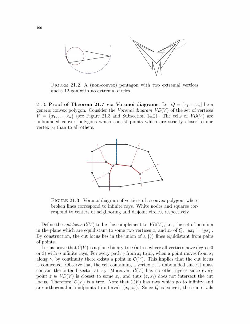
196

Figure 21.2. A (non-convex) pentagon with two extremal verticesand a 12-gon with no extremal circles.

21.3. Proof of Theorem 21.7 via Voronoi diagrams. Let Q = [x1 . . . xn] be ageneric convex polygon. Consider the Voronoi diagram VD(V ) of the set of verticesV = x1, . . . , xn (see Figure 21.3 and Subsection 14.2). The cells of VD(V ) areunbounded convex polygons which consist points which are strictly closer to onevertex xi than to all others.

Figure 21.3. Voronoi diagram of vertices of a convex polygon, wherebroken lines correspond to infinite rays. White nodes and squares cor-respond to centers of neighboring and disjoint circles, respectively.

Define the cut locus C(V ) to be the complement to VD(V ), i.e., the set of points yin the plane which are equidistant to some two vertices xi and xj of Q: |yxi| = |yxj|.By construction, the cut locus lies in the union of a

(n2

)lines equidistant from pairs

of points.Let us prove that C(V ) is a plane binary tree (a tree where all vertices have degree 0

or 3) with n infinite rays. For every path γ from xi to xj , when a point moves from xialong γ, by continuity there exists a point in C(V ). This implies that the cut locusis connected. Observe that the cell containing a vertex xi is unbounded since it mustcontain the outer bisector at xi. Moreover, C(V ) has no other cycles since everypoint z ∈ VD(V ) is closest to some xi, and thus (z, xi) does not intersect the cutlocus. Therefore, C(V ) is a tree. Note that C(V ) has rays which go to infinity andare orthogonal at midpoints to intervals (xi, xj). Since Q is convex, these intervals

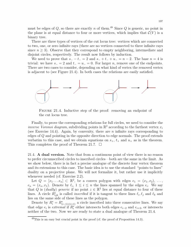
197

must be edges of Q, so there are exactly n of them.49 Since Q is generic, no point inthe plane is at equal distance to four or more vertices, which implies that C(V ) is abinary tree.

There are three types of vertices of the cut locus tree: vertices which are connectedto two, one, or zero infinite rays (there are no vertices connected to three infinite rayssince n ≥ 3). Observe that they correspond to empty neighboring, intermediate anddisjoint circles, respectively. The result now follows by induction.

We need to prove that s− − t− = 2 and s− + t− + u− = n − 2. The base n = 4 istrivial: we have s− = 2 and t− = u− = 0. For larger n, remove one of the endpoints.There are two cases to consider, depending on what kind of vertex the removed vertexis adjacent to (see Figure 21.4). In both cases the relations are easily satisfied.

Figure 21.4. Inductive step of the proof: removing an endpoint ofthe cut locus tree.

Finally, to prove the corresponding relations for full circles, we need to consider theinverse Voronoi diagram, subdividing points in R2 according to the farthest vertex xi(see Exercise 14.4). Again, by convexity, there are n infinite rays corresponding toedges of Q and pointing in the opposite direction to edge normals. The proof extendsverbatim to this case, and we obtain equations on s+, t+ and u+ as in the theorem.This completes the proof of Theorem 21.7.

21.4. A dual version. Note that from a continuous point of view there is no reasonto prefer circumscribed circles to inscribed circles—both are the same in the limit. Aswe show below, there is in fact a precise analogue of the discrete four vertex theoremand its extensions to this case. The basic idea is to use the standard “points to lines”duality on a projective plane. We will not formalize it, but rather use it implicitlywhenever needed (cf. Exercise 2.2).

Let Q = [x1 . . . xn] ⊂ R2, be a convex polygon with edges e1 = (x1, x2), . . . ,en = (xn, x1). Denote by ℓi, 1 ≤ i ≤ n the lines spanned by the edges ei. We saythat Q is (dually) generic if no point z ∈ R2 lies at equal distance to four of theselines. A circle R∗

ijk is called inscribed if it is tangent to three lines ℓi, ℓj and ℓk andlies on the same side of these lines as the polygon.

Denote by R∗i = R∗

(i−1)i(i+1) a circle inscribed into three consecutive lines. We saythat edge ei is extremal if R∗

i either intersects both edges ei−2 and ei+2, or intersectsneither of the two. Now we are ready to state a dual analogue of Theorem 21.4.

49This is an easy but crucial point in the proof (cf. the proof of Proposition 14.3).

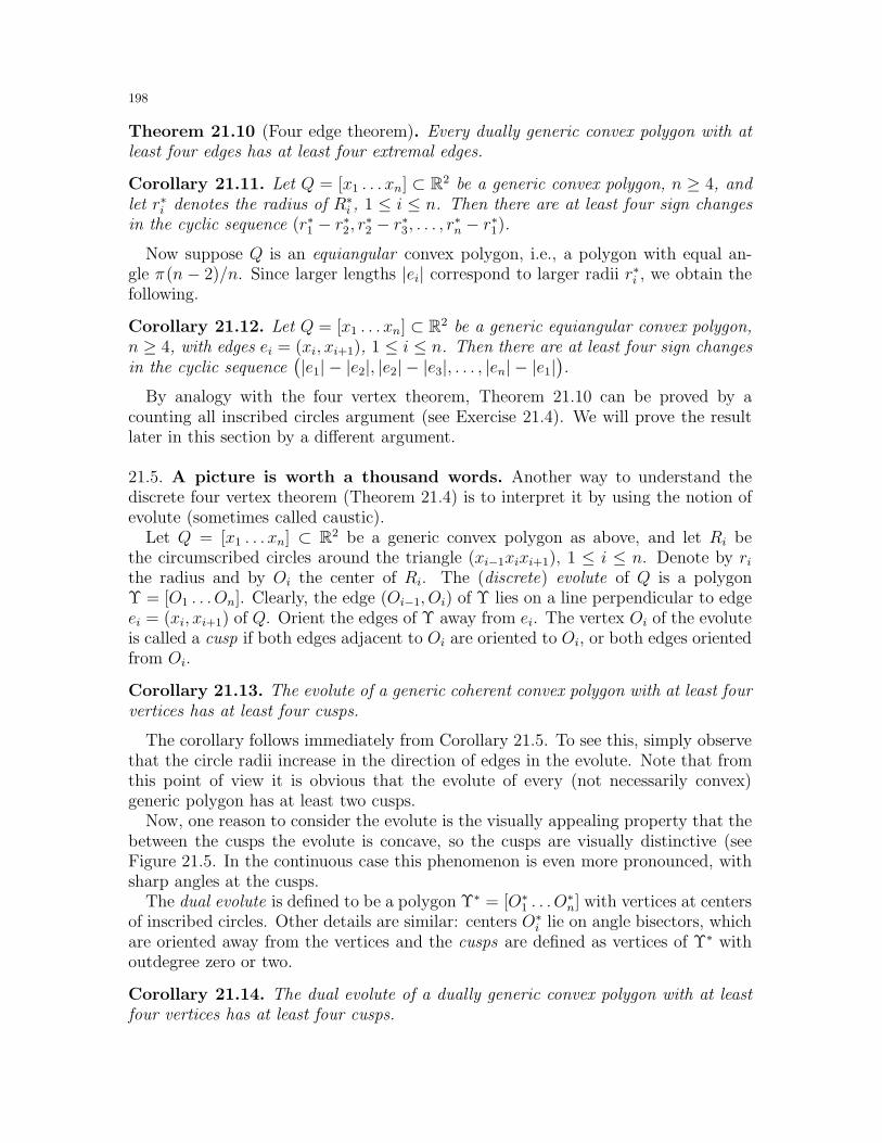
198

Theorem 21.10 (Four edge theorem). Every dually generic convex polygon with atleast four edges has at least four extremal edges.

Corollary 21.11. Let Q = [x1 . . . xn] ⊂ R2 be a generic convex polygon, n ≥ 4, andlet r∗i denotes the radius of R∗

i , 1 ≤ i ≤ n. Then there are at least four sign changesin the cyclic sequence (r∗1 − r∗2, r∗2 − r∗3, . . . , r∗n − r∗1).

Now suppose Q is an equiangular convex polygon, i.e., a polygon with equal an-gle π(n − 2)/n. Since larger lengths |ei| correspond to larger radii r∗i , we obtain thefollowing.

Corollary 21.12. Let Q = [x1 . . . xn] ⊂ R2 be a generic equiangular convex polygon,n ≥ 4, with edges ei = (xi, xi+1), 1 ≤ i ≤ n. Then there are at least four sign changesin the cyclic sequence

(|e1| − |e2|, |e2| − |e3|, . . . , |en| − |e1|

).

By analogy with the four vertex theorem, Theorem 21.10 can be proved by acounting all inscribed circles argument (see Exercise 21.4). We will prove the resultlater in this section by a different argument.

21.5. A picture is worth a thousand words. Another way to understand thediscrete four vertex theorem (Theorem 21.4) is to interpret it by using the notion ofevolute (sometimes called caustic).

Let Q = [x1 . . . xn] ⊂ R2 be a generic convex polygon as above, and let Ri bethe circumscribed circles around the triangle (xi−1xixi+1), 1 ≤ i ≤ n. Denote by rithe radius and by Oi the center of Ri. The (discrete) evolute of Q is a polygonΥ = [O1 . . . On]. Clearly, the edge (Oi−1, Oi) of Υ lies on a line perpendicular to edgeei = (xi, xi+1) of Q. Orient the edges of Υ away from ei. The vertex Oi of the evoluteis called a cusp if both edges adjacent to Oi are oriented to Oi, or both edges orientedfrom Oi.

Corollary 21.13. The evolute of a generic coherent convex polygon with at least fourvertices has at least four cusps.

The corollary follows immediately from Corollary 21.5. To see this, simply observethat the circle radii increase in the direction of edges in the evolute. Note that fromthis point of view it is obvious that the evolute of every (not necessarily convex)generic polygon has at least two cusps.

Now, one reason to consider the evolute is the visually appealing property that thebetween the cusps the evolute is concave, so the cusps are visually distinctive (seeFigure 21.5. In the continuous case this phenomenon is even more pronounced, withsharp angles at the cusps.

The dual evolute is defined to be a polygon Υ∗ = [O∗1 . . . O

∗n] with vertices at centers

of inscribed circles. Other details are similar: centers O∗i lie on angle bisectors, which

are oriented away from the vertices and the cusps are defined as vertices of Υ∗ withoutdegree zero or two.

Corollary 21.14. The dual evolute of a dually generic convex polygon with at leastfour vertices has at least four cusps.

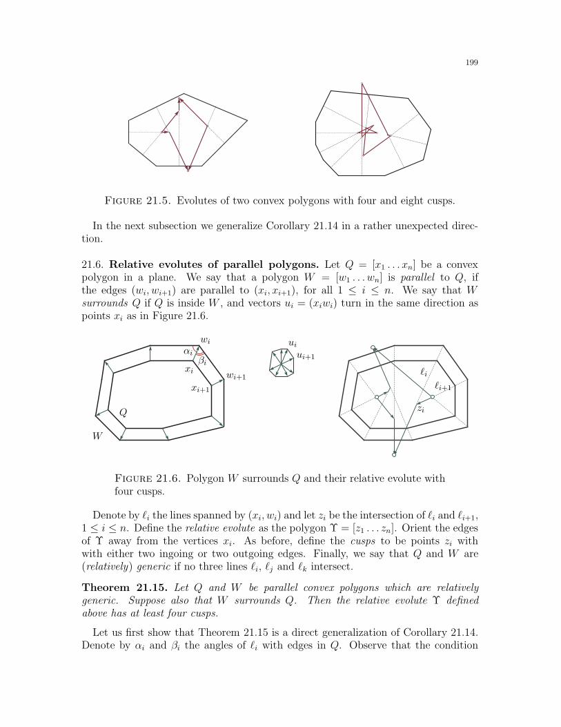
199

Figure 21.5. Evolutes of two convex polygons with four and eight cusps.

In the next subsection we generalize Corollary 21.14 in a rather unexpected direc-tion.

21.6. Relative evolutes of parallel polygons. Let Q = [x1 . . . xn] be a convexpolygon in a plane. We say that a polygon W = [w1 . . . wn] is parallel to Q, ifthe edges (wi, wi+1) are parallel to (xi, xi+1), for all 1 ≤ i ≤ n. We say that Wsurrounds Q if Q is inside W , and vectors ui = (xiwi) turn in the same direction aspoints xi as in Figure 21.6.

αiβi

xi

wi

xi+1

wi+1

Q

W

uiui+1

zi

ℓiℓi+1

Figure 21.6. Polygon W surrounds Q and their relative evolute withfour cusps.

Denote by ℓi the lines spanned by (xi, wi) and let zi be the intersection of ℓi and ℓi+1,1 ≤ i ≤ n. Define the relative evolute as the polygon Υ = [z1 . . . zn]. Orient the edgesof Υ away from the vertices xi. As before, define the cusps to be points zi withwith either two ingoing or two outgoing edges. Finally, we say that Q and W are(relatively) generic if no three lines ℓi, ℓj and ℓk intersect.

Theorem 21.15. Let Q and W be parallel convex polygons which are relativelygeneric. Suppose also that W surrounds Q. Then the relative evolute Υ definedabove has at least four cusps.

Let us first show that Theorem 21.15 is a direct generalization of Corollary 21.14.Denote by αi and βi the angles of ℓi with edges in Q. Observe that the condition

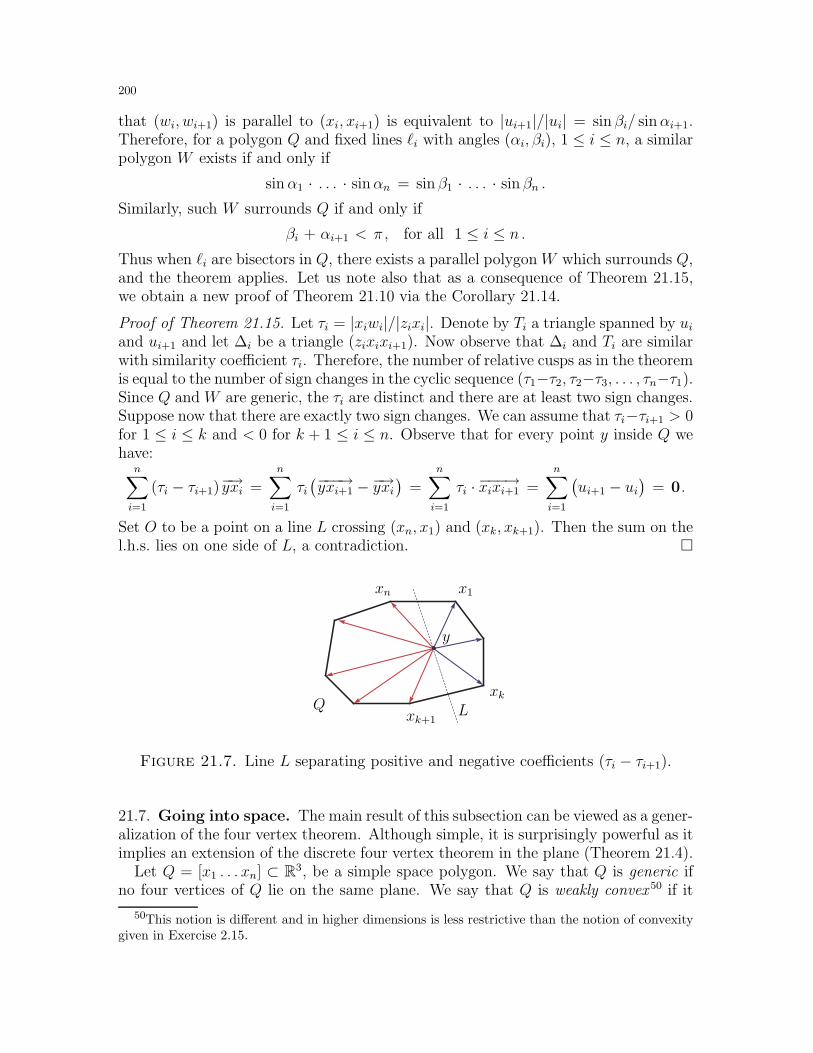
200

that (wi, wi+1) is parallel to (xi, xi+1) is equivalent to |ui+1|/|ui| = sin βi/ sinαi+1.Therefore, for a polygon Q and fixed lines ℓi with angles (αi, βi), 1 ≤ i ≤ n, a similarpolygon W exists if and only if

sinα1 · . . . · sinαn = sin β1 · . . . · sin βn .Similarly, such W surrounds Q if and only if

βi + αi+1 < π, for all 1 ≤ i ≤ n .

Thus when ℓi are bisectors in Q, there exists a parallel polygon W which surrounds Q,and the theorem applies. Let us note also that as a consequence of Theorem 21.15,we obtain a new proof of Theorem 21.10 via the Corollary 21.14.

Proof of Theorem 21.15. Let τi = |xiwi|/|zixi|. Denote by Ti a triangle spanned by uiand ui+1 and let ∆i be a triangle (zixixi+1). Now observe that ∆i and Ti are similarwith similarity coefficient τi. Therefore, the number of relative cusps as in the theoremis equal to the number of sign changes in the cyclic sequence (τ1−τ2, τ2−τ3, . . . , τn−τ1).Since Q and W are generic, the τi are distinct and there are at least two sign changes.Suppose now that there are exactly two sign changes. We can assume that τi−τi+1 > 0for 1 ≤ i ≤ k and < 0 for k + 1 ≤ i ≤ n. Observe that for every point y inside Q wehave:

n∑

i=1

(τi − τi+1)−→yxi =

n∑

i=1

τi(−−−→yxi+1 −−→yxi

)=

n∑

i=1

τi · −−−→xixi+1 =n∑

i=1

(ui+1 − ui

)= 0.

Set O to be a point on a line L crossing (xn, x1) and (xk, xk+1). Then the sum on thel.h.s. lies on one side of L, a contradiction.

x1

xk

xk+1

xn

Q

y

L

Figure 21.7. Line L separating positive and negative coefficients (τi − τi+1).

21.7. Going into space. The main result of this subsection can be viewed as a gener-alization of the four vertex theorem. Although simple, it is surprisingly powerful as itimplies an extension of the discrete four vertex theorem in the plane (Theorem 21.4).

Let Q = [x1 . . . xn] ⊂ R3, be a simple space polygon. We say that Q is generic ifno four vertices of Q lie on the same plane. We say that Q is weakly convex 50 if it

50This notion is different and in higher dimensions is less restrictive than the notion of convexitygiven in Exercise 2.15.

201

lies on the surface of the convex polytope P = conv(Q). We say that vertex xi is asupport vertex if (xi−1, xi, xi+1) is a face in P . In other words, the plane spanned byedges (xi−1, xi) and (xi, xi+1) is a supporting plane (see Figure 21.8).

Theorem 21.16 (Four support vertex theorem). Every generic weakly convex simplespace polygon with at least four vertices has at least four support vertices.

Proof. Let Q ⊂ R3 be the polygon as in the theorem. Since Q is generic, the polytopeP = conv(Q) is simplicial. Observe that Q is a Hamiltonian cycle in the graph Γof P . Thus, it divides the surface of S = ∂P into two triangulations T1 and T2, neitherof which have interior vertices. If Q has n ≥ 4 vertices, triangulations T1, T2 have(n−2) ≥ 2 triangles. Since the graph dual to T1 is a tree, it has at least two endpoints,i.e., T1 has at least two triangles (xi−1xixi+1) with two edges Q. This implies that T1

has at least two support vertices. Similarly, T2 also has two support vertices. Finally,note that these four support vertices must be distinct since otherwise they have degreetwo in Γ.

x1 x1

x2 x2

x3 x3

x4

x4x5

x5

x6 x6

Figure 21.8. Two weakly convex space polygons [x1 . . . x6] ⊂ R3, onewith four and another with six support vertices.

To see the connection to extremal circles in polygons, assume that a simplicialconvex polytope P ⊂ R3 as above is inscribed into a sphere. Then a circumscribedspherical circle around every triangular face (xi−1, xi, xi+1) is extremal, i.e., containsall remaining vertices on one side. Thus, one can think of Corollary 21.8 as a limitingcase of Theorem 21.16, when the circumscribed sphere becomes a plane.

Recall that a polygon Q ⊂ R2 is generic if no four points lie on a circle. We saythat Q is a Delaunay polygon if it is simple, generic, and for every edge (x, y) ∈ Qthere exists a circle R through x and y, such that the remaining vertices are eitherall inside of R or all outside of R.51 For example, every generic convex polygon is aDelaunay polygon.

Theorem 21.17. Every Delaunay polygon in the plane with at least four vertices hasat least four extremal circles.

51The name comes from Delaunay triangulations and the empty circle condition (see Section 14).

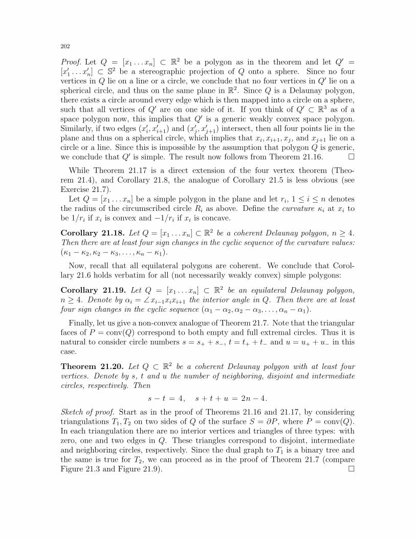
202

Proof. Let Q = [x1 . . . xn] ⊂ R2 be a polygon as in the theorem and let Q′ =[x′1 . . . x

′n] ⊂ S2 be a stereographic projection of Q onto a sphere. Since no four

vertices in Q lie on a line or a circle, we conclude that no four vertices in Q′ lie on aspherical circle, and thus on the same plane in R2. Since Q is a Delaunay polygon,there exists a circle around every edge which is then mapped into a circle on a sphere,such that all vertices of Q′ are on one side of it. If you think of Q′ ⊂ R3 as of aspace polygon now, this implies that Q′ is a generic weakly convex space polygon.Similarly, if two edges (x′i, x

′i+1) and (x′j , x

′j+1) intersect, then all four points lie in the

plane and thus on a spherical circle, which implies that xi, xi+1, xj , and xj+1 lie on acircle or a line. Since this is impossible by the assumption that polygon Q is generic,we conclude that Q′ is simple. The result now follows from Theorem 21.16.

While Theorem 21.17 is a direct extension of the four vertex theorem (Theo-rem 21.4), and Corollary 21.8, the analogue of Corollary 21.5 is less obvious (seeExercise 21.7).

Let Q = [x1 . . . xn] be a simple polygon in the plane and let ri, 1 ≤ i ≤ n denotesthe radius of the circumscribed circle Ri as above. Define the curvature κi at xi tobe 1/ri if xi is convex and −1/ri if xi is concave.

Corollary 21.18. Let Q = [x1 . . . xn] ⊂ R2 be a coherent Delaunay polygon, n ≥ 4.Then there are at least four sign changes in the cyclic sequence of the curvature values:(κ1 − κ2, κ2 − κ3, . . . , κn − κ1).

Now, recall that all equilateral polygons are coherent. We conclude that Corol-lary 21.6 holds verbatim for all (not necessarily weakly convex) simple polygons:

Corollary 21.19. Let Q = [x1 . . . xn] ⊂ R2 be an equilateral Delaunay polygon,n ≥ 4. Denote by αi = ∠xi−1xixi+1 the interior angle in Q. Then there are at leastfour sign changes in the cyclic sequence (α1 − α2, α2 − α3, . . . , αn − α1).

Finally, let us give a non-convex analogue of Theorem 21.7. Note that the triangularfaces of P = conv(Q) correspond to both empty and full extremal circles. Thus it isnatural to consider circle numbers s = s+ + s−, t = t+ + t− and u = u+ + u− in thiscase.

Theorem 21.20. Let Q ⊂ R2 be a coherent Delaunay polygon with at least fourvertices. Denote by s, t and u the number of neighboring, disjoint and intermediatecircles, respectively. Then

s − t = 4, s + t + u = 2n− 4.

Sketch of proof. Start as in the proof of Theorems 21.16 and 21.17, by consideringtriangulations T1, T2 on two sides of Q of the surface S = ∂P , where P = conv(Q).In each triangulation there are no interior vertices and triangles of three types: withzero, one and two edges in Q. These triangles correspond to disjoint, intermediateand neighboring circles, respectively. Since the dual graph to T1 is a binary tree andthe same is true for T2, we can proceed as in the proof of Theorem 21.7 (compareFigure 21.3 and Figure 21.9).

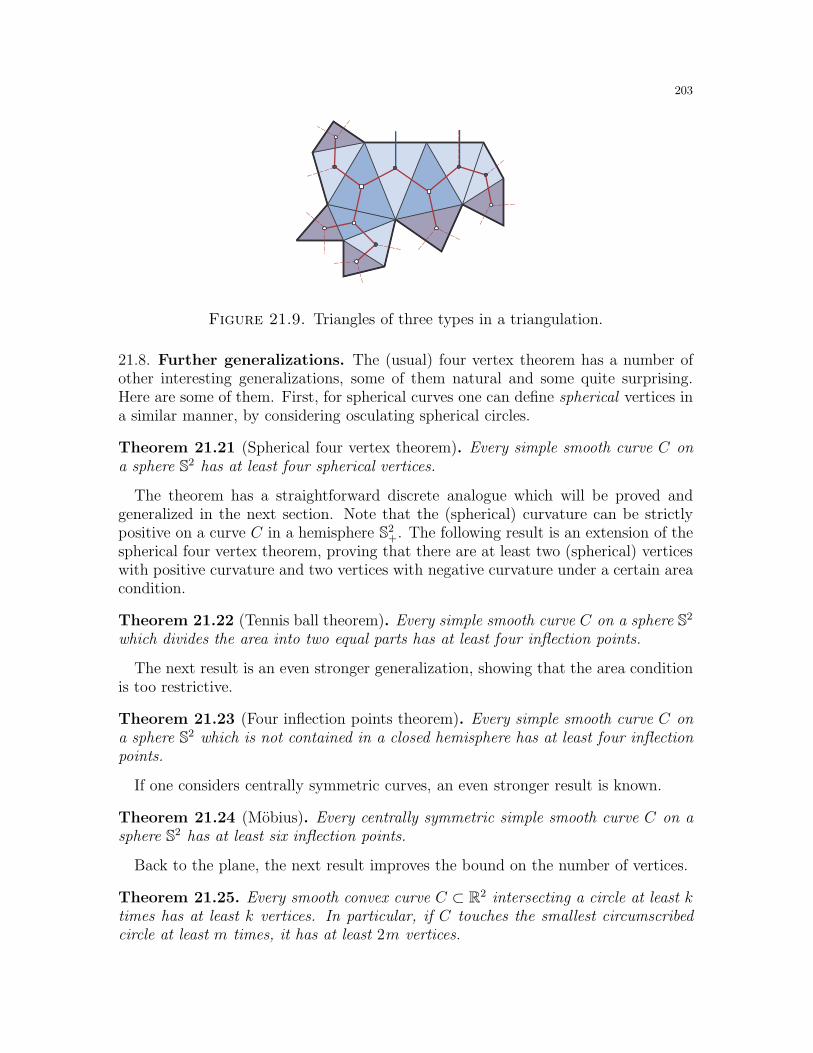
203

Figure 21.9. Triangles of three types in a triangulation.

21.8. Further generalizations. The (usual) four vertex theorem has a number ofother interesting generalizations, some of them natural and some quite surprising.Here are some of them. First, for spherical curves one can define spherical vertices ina similar manner, by considering osculating spherical circles.

Theorem 21.21 (Spherical four vertex theorem). Every simple smooth curve C ona sphere S2 has at least four spherical vertices.

The theorem has a straightforward discrete analogue which will be proved andgeneralized in the next section. Note that the (spherical) curvature can be strictlypositive on a curve C in a hemisphere S2

+. The following result is an extension of thespherical four vertex theorem, proving that there are at least two (spherical) verticeswith positive curvature and two vertices with negative curvature under a certain areacondition.

Theorem 21.22 (Tennis ball theorem). Every simple smooth curve C on a sphere S2

which divides the area into two equal parts has at least four inflection points.

The next result is an even stronger generalization, showing that the area conditionis too restrictive.

Theorem 21.23 (Four inflection points theorem). Every simple smooth curve C ona sphere S2 which is not contained in a closed hemisphere has at least four inflectionpoints.

If one considers centrally symmetric curves, an even stronger result is known.

Theorem 21.24 (Mobius). Every centrally symmetric simple smooth curve C on asphere S2 has at least six inflection points.

Back to the plane, the next result improves the bound on the number of vertices.

Theorem 21.25. Every smooth convex curve C ⊂ R2 intersecting a circle at least ktimes has at least k vertices. In particular, if C touches the smallest circumscribedcircle at least m times, it has at least 2m vertices.

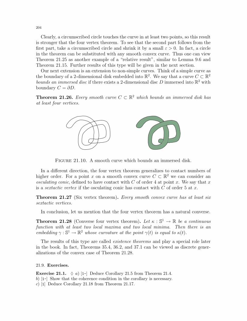
204

Clearly, a circumscribed circle touches the curve in at least two points, so this resultis stronger that the four vertex theorem. To see that the second part follows from thefirst part, take a circumscribed circle and shrink it by a small ε > 0. In fact, a circlein the theorem can be substituted with any smooth convex curve. Thus one can viewTheorem 21.25 as another example of a “relative result”, similar to Lemma 9.6 andTheorem 21.15. Further results of this type will be given in the next section.

Our next extension is an extension to non-simple curves. Think of a simple curve asthe boundary of a 2-dimensional disk embedded into R2. We say that a curve C ⊂ R2

bounds an immersed disc if there exists a 2-dimensional disc D immersed into R2 withboundary C = ∂D.

Theorem 21.26. Every smooth curve C ⊂ R2 which bounds an immersed disk hasat least four vertices.

Figure 21.10. A smooth curve which bounds an immersed disk.

In a different direction, the four vertex theorem generalizes to contact numbers ofhigher order. For a point x on a smooth convex curve C ⊂ R2 we can consider anosculating conic, defined to have contact with C of order 4 at point x. We say that xis a sextactic vertex if the osculating conic has contact with C of order 5 at x.

Theorem 21.27 (Six vertex theorem). Every smooth convex curve has at least sixsextactic vertices.

In conclusion, let us mention that the four vertex theorem has a natural converse.

Theorem 21.28 (Converse four vertex theorem). Let κ : S1 → R be a continuousfunction with at least two local maxima and two local minima. Then there is anembedding γ : S1 → R2 whose curvature at the point γ(t) is equal to κ(t).

The results of this type are called existence theorems and play a special role laterin the book. In fact, Theorems 35.4, 36.2, and 37.1 can be viewed as discrete gener-alizations of the convex case of Theorem 21.28.

21.9. Exercises.

Exercise 21.1. ♦ a) [1-] Deduce Corollary 21.5 from Theorem 21.4.b) [1-] Show that the coherence condition in the corollary is necessary.c) [1] Deduce Corollary 21.18 from Theorem 21.17.

205

Exercise 21.2. [1-] Let Q = [v1 . . . vn] ⊂ R2 be a convex polygon with equal angles.Suppose

|v1v2| ≤ |v2v3| ≤ . . . ≤ |vn−1vn| ≤ |vnv1|Prove that Q is a regular polygon.

Exercise 21.3. ♦ [1] Use limit argument to deduce Theorem 21.1 in full generality fromTheorem 21.17.

Exercise 21.4. [1+] The lines ℓi and ℓj are called adjacent if |i − j| = 1, i.e., they arespanned by adjacent edges. A circle R∗

ijk, i < j < k, is called distant if no two lines ℓi, ℓj , ℓkare adjacent, it is called mediocre if exactly one pair of lines is adjacent, and it is calledclose if two pairs of lines are adjacent. The circle R∗

ijk is called clear if it does not intersectany other lines, and it is called crossing if it intersects all other lines ℓm, m 6= i, j, k.

Let Q ⊂ R2 be a dually generic convex polygon with at least four vertices. Denote by s+,t+ and u+ the number of full close, distant and mediocre crossing circles, respectively.Similarly, denote by s−, t− and u− the number of close, distant and mediocre clear circles,respectively. Prove the following linear relations:

s+ − t+ = s− − t− = 2,

s+ + t+ + u+ = s− + t− + u− = n− 2.

Exercise 21.5. ♦ [1+] Find a dual version to Theorem 21.15, generalizing Corollary 21.13.

Exercise 21.6. [1] Show that when the number of vertices is odd, the dual evolute andorientation of its edges uniquely determine the convex polygon.

Exercise 21.7. ♦ [1] Deduce Corollary 21.18 from Theorem 21.17.

Exercise 21.8. ♦ [1] Use a limit argument to deduce Theorem 21.1 from Corollary 21.6when the curve is convex. Similarly, use Corollary 21.19 to deduce Theorem 21.1 in fullgenerality.

Exercise 21.9. [2-] Find and prove a discrete analogue of Theorem 21.21.

Exercise 21.10. [2-] Find and prove a discrete analogue of Theorem 21.22. Show that theresult is false for self-intersecting curves.

Exercise 21.11. [2] Find and prove a discrete analogue of Theorem 21.27.

Exercise 21.12. [2] Recall the cross-ratio of an ordered 4-tuple of distinct numbers, definedas

[a, b, c, d] =(a− c)(b− d)

(a− b)(c− d).

Let (x1, . . . , xn) and (y1, . . . , yn) be distinct real numbers, and let

αi = [xi, xi+1, xi+2, xi+3], βi = [yi, yi+1, yi+2, yi+3],

where, all indices are taken modulo n. Prove that a cyclic sequence (α1 − β1, . . . , αn − βn)has at least four sign changes.

Exercise 21.13. a) [2-] Prove that every smooth convex curve C in the plane has at leastthree pairs of opposite points (points with parallel tangents) which have equal curvature.b) [∗] Find a discrete analogue of part a).

206

21.10. Final remarks. The four vertex theorem (Theorem 21.1) is a classical result inDifferential Geometry, available in numerous textbooks and survey articles (see e.g., [Cher,Gug1]). It was proved by Mukhopadhyaya for convex curves (1909) and by A. Kneser infull generality (1912). Theorem 21.2 is due to H. Kneser (1922), the son of A. Kneser, andTheorem 21.3 is due to Bose (1932).

Interestingly, a related result of Mobius (Theorem 21.24) is much older (1852). For thehistory of the four vertex theorem, various extensions and references see [DGPV, Mus4,Ume, Weg2] and [OT2, Chapter 4].

Corollary 21.6 and Corollary 21.5 for obtuse polygons are due to S. Bilinski (1961, 1963).The general version of Corollary 21.5 is due to Musin (see [Mus1] for an introduction and anelementary proof). Theorem 21.7 can be viewed as the most general discrete Bose theorem,and is a variation on several known results (see e.g., Theorem 1.7 in [Mus4]). The proof ofTheorem 21.7 is new in this form. It uses the cut locus idea in the Rene Thom’s proof (1972)of the four vertex theorem (see [Ume]), subsequently repeatedly rediscovered and adaptedto polygons (see [BanG, Weg2, Weg4]). The four edge theorem (Theorem 21.10) seems tobe new. In computational geometry the cut locus is well studied under the name medialaxis [AurK].

Theorem 21.15 and the proof in Subsection 21.5 are due to Tabachnikov [Tab4]. Theo-rems 21.16 and 21.17 are due to Sedykh [Sed] (a version of Corollary 21.19 was also dis-covered by Dahlberg). Interestingly, there is also a two vertex theorem for general Jordancurves [Hau].

Theorem 21.23 was first proved by Segre (1968), but a version of it was stated by Blaschkeas an exercise in [Bla1]. Its corollary, the tennis ball theorem (Theorem 21.22) was discov-ered, aptly named and popularized by Arnold [Arn1, §20]. There is a great deal of literatureon these results and their various generalizations (see [Arn3, pp. 99, 553] for a short surveyand further references).

The first part of Theorem 21.25 goes back to Blaschke (1916) and Mukhopadhyaya (1931)(see also [Bla3]). It was rediscovered several times with the definitive version due to Jack-son [Jac]52. The second part is an easy corollary of the first and was popularized in [Oss]).Similarly, the six vertex theorem (Theorem 21.27) was proved by Mukhopadhyaya in hisoriginal paper (1909), and was repeatedly rediscovered. For more on the history and ad-vanced generalizations, including common generalizations with the Mobius theorem andconnections to classical Cayley’s results, see [ThoU].

Theorem 21.26 is due to Pinkall [Pink] who proved it in the generality of all immersed

surfaces. The converse of the four vertex theorem (Theorem 21.28) was proved by Gluck

for convex curves (1971), and by Dahlberg in full generality (1997, published posthumously

in 2005, see [DGPV]). We should mention that much of the difficulty in the proof is

analytical and we are not aware of a nontrivial discrete version.

52References to older results, mostly in German, can be found in the AMS Math. Reviews on [Jac].

207

22. Relative geometry of convex polygons

Here we continue our study of four vertex theorems, shifting in the direction oftheir relative geometry. We limit our scope and concentrate only on results whichwill be used later on, in the proof of rigidity results of convex polyhedra.

22.1. The Legendre–Cauchy lemma. We start with the following classical resultwhich can be viewed as relative versions of the four vertex theorem (Theorem 21.4).

Theorem 22.1 (Legendre–Cauchy lemma). Let Q = [v1 . . . vn] and Q′ = [v′1 . . . v′n]

be two convex polygons in the plane with equal corresponding edge lengths: |vivi+1| =|v′iv′i+1|. Denote by αi = ∠vi−1vivi+1 and βi = ∠v′i−1v

′iv

′i+1 the angles in the polygons,

where 1 ≤ i ≤ n and the indices are taken modulo n. Then either there are at leastfour sign changes in the cyclic sequence (α1 − β1, . . . , αn − βn), or the sequence iszero.

To see the connection to the four vertex theorem, consider the case of equilateralpolygons Q = [v1v2 . . . vn] and Q′ = [v2 . . . vnv1]. The theorem implies in this casethat either all corresponding angles are equal, or there are at least four sign changesin the sequence (α1 − α2, . . . , αn − α1). This is a minor variation on Corollary 21.6.

Let us immediately state a spherical version of the theorem, which will prove usefulin the proof of the Cauchy theorem (see Section 26).

Theorem 22.2 (Spherical Legendre–Cauchy lemma). Let Q = [x1 . . . xn] and Q′ =[x′1 . . . x

′n] be two spherical convex polygons on a hemisphere S+ with equal corre-

sponding edge lengths: |xixi+1|S2 = |x′ix′i+1|S2. Denote by αi = ∢vi−1vivi+1 and βi =∢v′i−1v

′iv

′i+1 the spherical angles in the polygons, 1 ≤ i ≤ n. Then either there are at

least four sign changes in the cyclic sequence (α1 − β1, . . . , αn − βn), or the sequenceis zero.

One can think of this result as a generalization of Theorem 22.1 since the planepolygons are the limits of spherical polygons, as the radius of a sphere tends to infinity.Later in this section we prove both result by the same general argument.

Note that the condition that both polygons lie inside a hemisphere S+ is necessary,since otherwise one can find two spherical triangles with equal corresponding sidesand all angles of the first strictly smaller than the corresponding angles of the secondtriangle. For example, take any small spherical triangle ∆ and its complement ∆′ =S2r∆. The angles of ∆ are < π, while the angles of ∆′ are > π. Similarly, as can beseen already for two quadrilaterals in Figure 22.1, the result is false for non-convexpolygons.

22.2. Making errors at all the right places. The proof of the Legendre-Cauchylemma is elementary, but delicate at one point. The original proof, which by nowhas become standard, contained a famous error which eluded discovery for nearlya century and has led to a number of interesting (and correct) results. Thus westart with the original proof, then point out the famous error, and then correct it.The reader might want to pay extra attention to the figures and think it over beforelearning the answer.

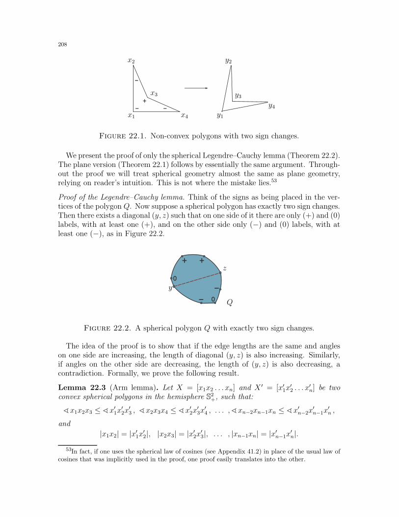
208

-

+

- -

x1

x2

x3

x4 y1

y2

y3

y4

Figure 22.1. Non-convex polygons with two sign changes.

We present the proof of only the spherical Legendre–Cauchy lemma (Theorem 22.2).The plane version (Theorem 22.1) follows by essentially the same argument. Through-out the proof we will treat spherical geometry almost the same as plane geometry,relying on reader’s intuition. This is not where the mistake lies.53

Proof of the Legendre–Cauchy lemma. Think of the signs as being placed in the ver-tices of the polygon Q. Now suppose a spherical polygon has exactly two sign changes.Then there exists a diagonal (y, z) such that on one side of it there are only (+) and (0)labels, with at least one (+), and on the other side only (−) and (0) labels, with atleast one (−), as in Figure 22.2.

-

-

0

+

0

+

y

z

Q

Figure 22.2. A spherical polygon Q with exactly two sign changes.

The idea of the proof is to show that if the edge lengths are the same and angleson one side are increasing, the length of diagonal (y, z) is also increasing. Similarly,if angles on the other side are decreasing, the length of (y, z) is also decreasing, acontradiction. Formally, we prove the following result.

Lemma 22.3 (Arm lemma). Let X = [x1x2 . . . xn] and X ′ = [x′1x′2 . . . x

′n] be two

convex spherical polygons in the hemisphere S2+, such that:

∢x1x2x3 ≤ ∢x′1x′2x

′3 , ∢x2x3x4 ≤ ∢x′2x

′3x

′4 , . . . ,∢xn−2xn−1xn ≤ ∢x′n−2x

′n−1x

′n ,

and

|x1x2| = |x′1x′2|, |x2x3| = |x′2x′3|, . . . , |xn−1xn| = |x′n−1x′n|.

53In fact, if one uses the spherical law of cosines (see Appendix 41.2) in place of the usual law ofcosines that was implicitly used in the proof, one proof easily translates into the other.

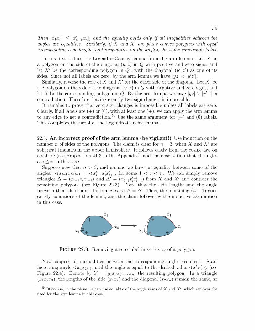
209

Then |x1xn| ≤ |x′n−1x′n|, and the equality holds only if all inequalities between the

angles are equalities. Similarly, if X and X ′ are plane convex polygons with equalcorresponding edge lengths and inequalities on the angles, the same conclusion holds.

Let us first deduce the Legendre–Cauchy lemma from the arm lemma. Let X bea polygon on the side of the diagonal (y, z) in Q with positive and zero signs, andlet X ′ be the corresponding polygon in Q′, with the diagonal (y′, z′) as one of itssides. Since not all labels are zero, by the arm lemma we have |yz| < |y′z′|.

Similarly, reverse the role of X and X ′ for the other side of the diagonal. Let X ′ bethe polygon on the side of the diagonal (y, z) in Q with negative and zero signs, andlet X be the corresponding polygon in Q. By the arm lemma we have |yz| > |y′z′|, acontradiction. Therefore, having exactly two sign changes is impossible.

It remains to prove that zero sign changes is impossible unless all labels are zero.Clearly, if all labels are (+) or (0), with at least one (+), we can apply the arm lemmato any edge to get a contradiction.54 Use the same argument for (−) and (0) labels.This completes the proof of the Legendre-Cauchy lemma.

22.3. An incorrect proof of the arm lemma (be vigilant!) Use induction on thenumber n of sides of the polygons. The claim is clear for n = 3, when X and X ′ arespherical triangles in the upper hemisphere. It follows easily from the cosine law ona sphere (see Proposition 41.3 in the Appendix), and the observation that all anglesare ≤ π in this case.

Suppose now that n > 3, and assume we have an equality between some of theangles: ∢xi−1xixi+1 = ∢x′i−1x

′ix

′i+1, for some 1 < i < n. We can simply remove

triangles ∆ = (xi−1xixi+1) and ∆′ = (x′i−1x′ix

′i+1) from X and X ′ and consider the

remaining polygons (see Figure 22.3). Note that the side lengths and the anglebetween them determine the triangles, so ∆ = ∆′. Thus, the remaining (n− 1)-gonssatisfy conditions of the lemma, and the claim follows by the inductive assumptionin this case.

+ +0

+

+ +

+

x1 x1

xn xnxi xi

Figure 22.3. Removing a zero label in vertex xi of a polygon.

Now suppose all inequalities between the corresponding angles are strict. Startincreasing angle ∢x1x2x3 until the angle is equal to the desired value ∢x′1x

′2x

′3 (see

Figure 22.4). Denote by Y = [y1x2x3 . . . xn] the resulting polygon. In a triangle(x1x2x3), the lengths of the side (x1x2) and the diagonal (x2xn) remain the same, so

54Of course, in the plane we can use equality of the angle sums of X and X ′, which removes theneed for the arm lemma in this case.

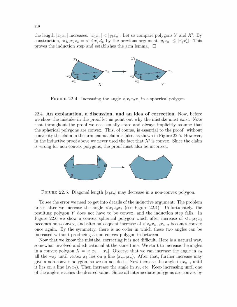
210

the length |x1xn| increases: |x1xn| < |y1xn|. Let us compare polygons Y and X ′. Byconstruction, ∢y1x2x3 = ∢x′1x

′2x

′3, by the previous argument |y1xn| ≤ |x′1x′n|. This

proves the induction step and establishes the arm lemma.

0

+ +++ +

X Y

x1y1

xn xnx2 x2

x3 x3

Figure 22.4. Increasing the angle ∢x1x2x3 in a spherical polygon.

22.4. An explanation, a discussion, and an idea of correction. Now, beforewe show the mistake in the proof let us point out why the mistake must exist. Notethat throughout the proof we occasionally state and always implicitly assume thatthe spherical polygons are convex. This, of course, is essential to the proof: withoutconvexity the claim in the arm lemma claim is false, as shown in Figure 22.5. However,in the inductive proof above we never used the fact that X ′ is convex. Since the claimis wrong for non-convex polygons, the proof must also be incorrect.

+ +

0 0

0 0

--

Figure 22.5. Diagonal length |x1xn| may decrease in a non-convex polygon.

To see the error we need to get into details of the inductive argument. The problemarises after we increase the angle ∢x1x2x3 (see Figure 22.4). Unfortunately, theresulting polygon Y does not have to be convex, and the induction step fails. InFigure 22.6 we show a convex spherical polygon which after increase of ∢x1x2x3

becomes non-convex, and after subsequent increase of ∢xnxn−1xn−2 becomes convexonce again. By the symmetry, there is no order in which these two angles can beincreased without producing a non-convex polygon in between.

Now that we know the mistake, correcting it is not difficult. Here is a natural way,somewhat involved and educational at the same time. We start to increase the anglesin a convex polygon X = [x1x2 . . . xn]. Observe that we can increase the angle in x2

all the way until vertex x1 lies on a line (xn−1xn). After that, further increase maygive a non-convex polygon, so we do not do it. Now increase the angle in xn−1 untilit lies on a line (x1x2). Then increase the angle in x2, etc. Keep increasing until oneof the angles reaches the desired value. Since all intermediate polygons are convex by

211

+ + +

X Y X ′

x1

x2 x2

x3 x3

y1 x′1xn xn

xn−1

x′n

Figure 22.6. Increasing angle ∢x1x2x3 may result in a non-convex polygon.

construction, the distance |x1xn| will only increase by the argument as in the proofabove.

The trouble with this argument is that it requires an unbounded number of steps (aslong as this number is finite it is not really a problem), and that it takes some work toshow that the increase in the angles does not converge to a value lower than necessary(see Figure 22.7). This latter part is trickier and uses convexity of X ′; it is left to thereader. Once all the details are set and done, one would really want a different proofof the arm lemma, somewhat simpler even if perhaps not as straightforward (see alsoSubsection 23.5).

+ +

Figure 22.7. The iterative process of increasing two angles.

22.5. All’s well that ends well. Based on the first impression one would assumethat the arm lemma is obvious. After some thinking and working out the iterativeargument above one can conclude that it is inherently complicated. Well, one wouldbe wrong again. Here is a simple and ingenious inductive proof of the arm lemma.

Proof of the arm lemma (for real now! ). Use induction on n. As in the argumentabove, we can assume that all angles of X as in the lemma are strictly increasing.The base n = 3 for triangles is also established. The argument in the original prooffails if there exists a polygon Y = [y1x2 . . . xn] where ∢x′1x

′2x

′3 > ∢y1x2x3 ≥ ∢x1x2x3,

and point y1 lies on the (xn−1xn) line. Apply the base of induction to go from X to Y :in the triangle (x1x2x3) we have |y1xn| ≥ |x1xn|.

Think of Y as (n − 1)-gon with one side comprised of two: |y1xn−1| = |y1xn| +|xn−1xn|. Let Z = [x′1x

′2 . . . x

′n−1] be a (n − 1)-gon with sides and angles as in the

lemma. By inductive assumption, going from Y to Z, we have |x′1x′n−1| ≥ |y1xn−1|.

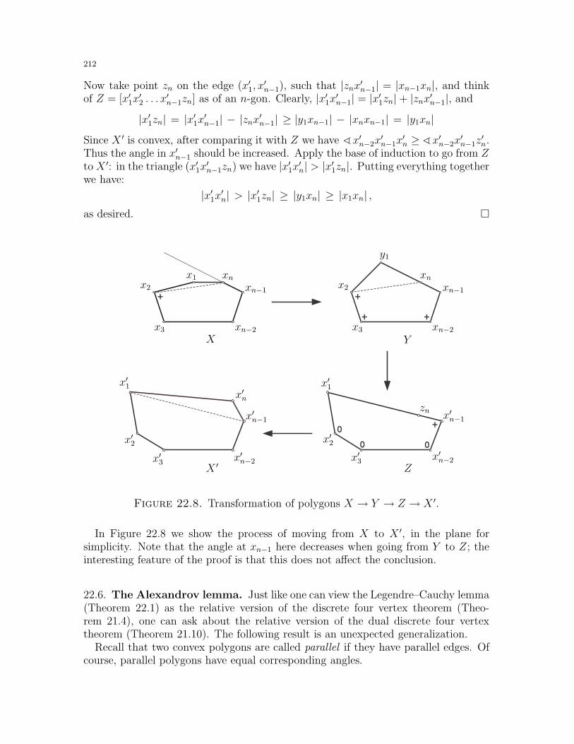
212

Now take point zn on the edge (x′1, x′n−1), such that |znx′n−1| = |xn−1xn|, and think

of Z = [x′1x′2 . . . x

′n−1zn] as of an n-gon. Clearly, |x′1x′n−1| = |x′1zn|+ |znx′n−1|, and

|x′1zn| = |x′1x′n−1| − |znx′n−1| ≥ |y1xn−1| − |xnxn−1| = |y1xn|Since X ′ is convex, after comparing it with Z we have ∢x′n−2x

′n−1x

′n ≥ ∢x′n−2x

′n−1z

′n.

Thus the angle in x′n−1 should be increased. Apply the base of induction to go from Zto X ′: in the triangle (x′1x

′n−1zn) we have |x′1x′n| > |x′1zn|. Putting everything together

we have:

|x′1x′n| > |x′1zn| ≥ |y1xn| ≥ |x1xn| ,as desired.

+

++

+

+

00

0

X Y

ZX ′

x1x2x2

x3x3 xn−2xn−2

xn−1xn−1

xnxn

y1

x′1 x′1

x′2 x′2

x′3 x′3x′n−2 x′n−2

x′n−1 x′n−1

zn

x′n

Figure 22.8. Transformation of polygons X → Y → Z → X ′.

In Figure 22.8 we show the process of moving from X to X ′, in the plane forsimplicity. Note that the angle at xn−1 here decreases when going from Y to Z; theinteresting feature of the proof is that this does not affect the conclusion.

22.6. The Alexandrov lemma. Just like one can view the Legendre–Cauchy lemma(Theorem 22.1) as the relative version of the discrete four vertex theorem (Theo-rem 21.4), one can ask about the relative version of the dual discrete four vertextheorem (Theorem 21.10). The following result is an unexpected generalization.

Recall that two convex polygons are called parallel if they have parallel edges. Ofcourse, parallel polygons have equal corresponding angles.

213

Theorem 22.4 (Alexandrov lemma). Let X = [x1 . . . xn] and Y = [y1 . . . yn] be twoparallel convex polygons in the plane. Denote by ai and bi the edge lengths in X and Y ,respectively. Suppose neither X fits inside Y , nor Y fits inside X by a translation.Then either there are at least four sign changes in the cyclic sequence (a1−b1, . . . , an−bn), or the sequence is zero.

The condition that neither polygon fits inside another may seem unusual, as thereis no such condition in Theorem 22.1. In fact, without this condition the claim isfalse (see Figure 22.9).

+

+

+

+ +

-

XX

Y

Figure 22.9. Parallel hexagons with exactly two sign changes.

The connection to the dual discrete four vertex theorem is similar to the case ofthe Legendre–Cauchy lemma. Consider an equiangular polygon X = [x1 . . . xn] and apolygon Y obtained from X by a clockwise 2π/n rotation. If X = Y , the sequence inthe theorem is a zero sequence. Otherwise, since area(X) = area(Y ), neither polygonfits inside another, and the cyclic sequence (a1 − a2, . . . , an − a1) has at least foursign changes. Thus we obtain Corollary 21.12. Here is a more general corollary fromAlexandrov’s lemma.

Corollary 22.5. Let X = [x1 . . . xn] and Y = [y1 . . . yn] be two parallel convex poly-gons in the plane. Denote by ai and bi the edge lengths in X and Y , respectively.Suppose either of the following conditions holds:

(i) area(X) = area(Y ),(ii) perimeter(X) = perimeter(Y ).

Then either there are at least four sign changes in the cyclic sequence (a1−b1, . . . , an−bn), or the sequence is zero.

The follows from the Alexandrov lemma since under either of these conditionsneither polygon fits inside another (for the perimeter see part a of Exercise 7.11). Ofcourse, one can replace the area and perimeter in (i), (ii) with any other function fof the polygons which satisfies: f(X) ≤ f(Y ) for all X ⊆ Y , where the equality holdsonly if X = Y . For example, take any polynomial of area(X) and perimeter(X) withpositive coefficients. Alternatively, one can use two asymmetric conditions, such as,e.g., diam(X) < diam(Y ) and width(X) > width(Y ).

The proof of the Alexandrov lemma is elementary but tedious. Instead, we proveonly the second part of the corollary.

Proof of part (ii) of Corollary 22.5. Let e i = −−−→xixi+1 be an edge vector in X, and letu i = e i/ai be a unit vector in direction e i, 1 ≤ i ≤ n. Since these unit vectors are

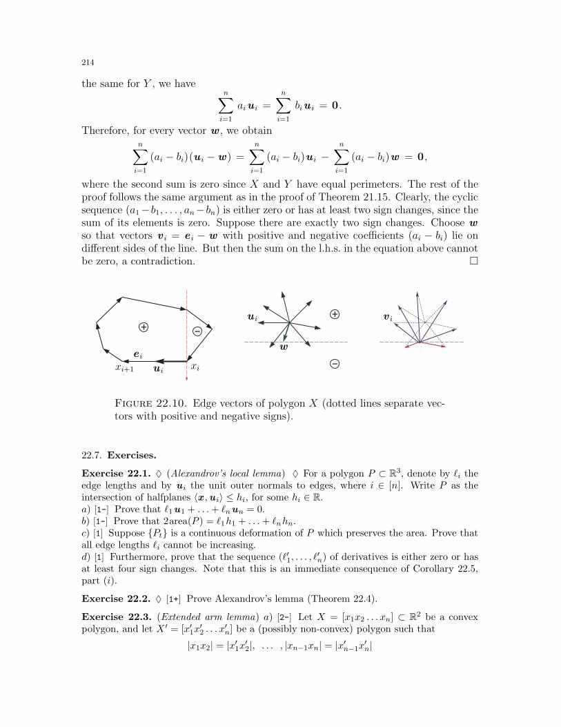
214

the same for Y , we haven∑

i=1

aiu i =

n∑

i=1

biu i = 0.

Therefore, for every vector w , we obtainn∑

i=1

(ai − bi)(u i −w) =

n∑

i=1

(ai − bi)u i −n∑

i=1

(ai − bi)w = 0,

where the second sum is zero since X and Y have equal perimeters. The rest of theproof follows the same argument as in the proof of Theorem 21.15. Clearly, the cyclicsequence (a1−b1, . . . , an−bn) is either zero or has at least two sign changes, since thesum of its elements is zero. Suppose there are exactly two sign changes. Choose w

so that vectors v i = e i − w with positive and negative coefficients (ai − bi) lie ondifferent sides of the line. But then the sum on the l.h.s. in the equation above cannotbe zero, a contradiction.

-+

+

-

e i

u i

u i

v i

w

xixi+1

Figure 22.10. Edge vectors of polygon X (dotted lines separate vec-tors with positive and negative signs).

22.7. Exercises.

Exercise 22.1. ♦ (Alexandrov’s local lemma) ♦ For a polygon P ⊂ R3, denote by ℓi theedge lengths and by u i the unit outer normals to edges, where i ∈ [n]. Write P as theintersection of halfplanes 〈x ,u i〉 ≤ hi, for some hi ∈ R.a) [1-] Prove that ℓ1u1 + . . .+ ℓnun = 0.b) [1-] Prove that 2area(P ) = ℓ1h1 + . . .+ ℓnhn.c) [1] Suppose Pt is a continuous deformation of P which preserves the area. Prove thatall edge lengths ℓi cannot be increasing.d) [1] Furthermore, prove that the sequence (ℓ′1, . . . , ℓ

′n) of derivatives is either zero or has

at least four sign changes. Note that this is an immediate consequence of Corollary 22.5,part (i).

Exercise 22.2. ♦ [1+] Prove Alexandrov’s lemma (Theorem 22.4).

Exercise 22.3. (Extended arm lemma) a) [2-] Let X = [x1x2 . . . xn] ⊂ R2 be a convexpolygon, and let X ′ = [x′1x

′2 . . . x

′n] be a (possibly non-convex) polygon such that

|x1x2| = |x′1x′2|, . . . , |xn−1xn| = |x′n−1x′n|

215

and

|π − ∠x1x2x3| ≥ |π − ∠x′1x′2x

′3| , . . . , |π − ∠xn−2xn−1xn| ≥ |π − ∠x′n−2x

′n−1x

′n| .

Then |x1xn| ≤ |x′n−1x′n|.

b) [1+] What happens for X ⊂ R3?

Exercise 22.4. (Line development) a) [2-] Let P ⊂ R3 be a convex polytope and letA ⊂ ∂P be a convex polygon on the surface of P , defined as a polygonal region with allinterior angles satisfying 0 ≤ αi ≤ π. Let Q = ∂A. Unfold the faces of F containing Qonto a plane, starting with any one of them, in the order of intersection with Q (note that,generally speaking, Q might go though the same facet more than once). Prove the unfoldingof Q is not self-intersecting.55

b) [1] Let P ⊂ R3 be a convex polytope and let L be a plane which does not contain verticesof P . Consider the curve C = L ∩ ∂P . Prove the unfolding of C is not self-intersecting.

22.8. Final remarks. While the arm lemma (Lemma 22.3) seem to be due to Legendre,it is rarely attributed to him [Sab6]. It became famous in Cauchy’s original proof of therigidity of convex polytopes (see Section 26). In any case, the mistake was discovered andcorrected only by Steinitz in the 1920’s (see Steinitz’s proof in [Lyu]). The mistake is sosubtle and occurs in such an ‘obvious’ claim, a number of textbooks continue to repeatit until this day. Since Steinitz, a number of correct proofs of the arm lemma have beenproposed, some simpler and more elegant than others (compare the proofs in [A2, Ber1,Hada, Lyu, Sab6, SchoZ, Sto] and try not to be awed). The concise (and correct) proof ofthe arm lemma given in Subsection 22.5 was discovered in [SchoZ] (see also [AigZ, §11]).By now there are a number of papers completely dedicated to the arm lemma and itsgeneralization (see [Sab6, Schl4] and references in [Con5]). We should mention here thatthe Pogorelov lemma (Lemma 28.5) can be viewed as another variation on the arm lemma.

Let us note that the arm lemma is more transparent and easier to prove in the plane thanon a sphere (see e.g. the first proof in [SchoZ]), thus several authors gave a correct proof ofa plane version, and then mislead the reader by saying that the proof in the spherical caseis “almost the same”. The reader should be careful with such claims.

The proof of the Alexandrov lemma (Theorem 22.4) is elementary and can be found

in [A2, §6.1] and [Lyu].56 The lemma is used in Section 36 in the elementary proof of the

Minkowski theorem (Theorem 36.2) in R3 (see also Exercise 36.4). The elegant proof of

the infinitesimal analogue of part (i) is given in Exercise 22.1 (see [A2, §9.1] and a concise

presentation in Alexandrov’s original 1937 article). The proof of part (ii) of Corollary 22.5

is new.

55If one imagines rolling a die of shape P on a plane, the unfolding of Q is the trace left by Q.See Section 40 for more on unfoldings.

56A simpler proof was recently found by Gunter Rote (personal communication).

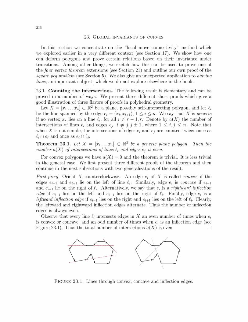
216

23. Global invariants of curves

In this section we concentrate on the “local move connectivity” method whichwe explored earlier in a very different context (see Section 17). We show how onecan deform polygons and prove certain relations based on their invariance undertransitions. Among other things, we sketch how this can be used to prove one ofthe four vertex theorem extensions (see Section 21) and outline our own proof of thesquare peg problem (see Section 5). We also give an unexpected application to halvinglines, an important subject, which we do not explore elsewhere in the book.

23.1. Counting the intersections. The following result is elementary and can beproved in a number of ways. We present three different short proofs which give agood illustration of three flavors of proofs in polyhedral geometry.

Let X = [x1 . . . xn] ⊂ R2 be a plane, possibly self-intersecting polygon, and let ℓibe the line spanned by the edge ei = (xi, xi+1), 1 ≤ i ≤ n. We say that X is genericif no vertex xr lies on a line ℓi, for all i 6= r − 1, r. Denote by a(X) the number ofintersections of lines ℓi and edges ej , i 6= j, j ± 1, where 1 ≤ i, j ≤ n. Note thatwhen X is not simple, the intersections of edges ei and ej are counted twice: once asℓi ∩ ej and once as ei ∩ ℓj.Theorem 23.1. Let X = [x1 . . . xn] ⊂ R2 be a generic plane polygon. Then thenumber a(X) of intersections of lines ℓi and edges ej is even.

For convex polygons we have a(X) = 0 and the theorem is trivial. It is less trivialin the general case. We first present three different proofs of the theorem and thencontinue in the next subsections with two generalizations of the result.

First proof. Orient X counterclockwise. An edge ei of X is called convex if theedges ei−1 and ei+1 lie on the left of line ℓi. Similarly, edge ei is concave if ei−1

and ei+1 lie on the right of ℓi. Alternatively, we say that ei is a rightward inflectionedge if ei−1 lies on the left and ei+1 lies on the right of ℓi. Finally, edge ei is aleftward inflection edge if ei−1 lies on the right and ei+1 lies on the left of ℓi. Clearly,the leftward and rightward inflection edges alternate. Thus the number of inflectionedges is always even.

Observe that every line ℓi intersects edges in X an even number of times when eiis convex or concave, and an odd number of times when ei is an inflection edge (seeFigure 23.1). Thus the total number of intersections a(X) is even.

Figure 23.1. Lines through convex, concave and inflection edges.

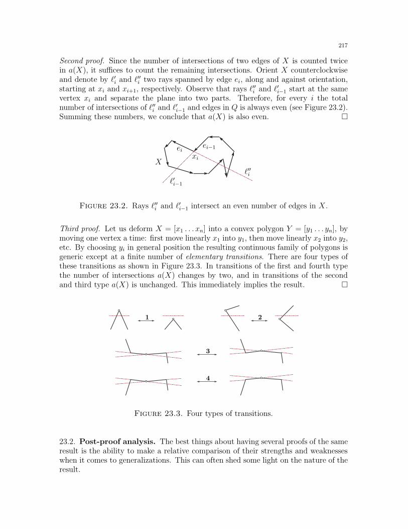
217

Second proof. Since the number of intersections of two edges of X is counted twicein a(X), it suffices to count the remaining intersections. Orient X counterclockwiseand denote by ℓ′i and ℓ′′i two rays spanned by edge ei, along and against orientation,starting at xi and xi+1, respectively. Observe that rays ℓ′′i and ℓ′i−1 start at the samevertex xi and separate the plane into two parts. Therefore, for every i the totalnumber of intersections of ℓ′′i and ℓ′i−1 and edges in Q is always even (see Figure 23.2).Summing these numbers, we conclude that a(X) is also even.

Xxi

eiei−1

ℓ′i−1

ℓ′′i

Figure 23.2. Rays ℓ′′i and ℓ′i−1 intersect an even number of edges in X.

Third proof. Let us deform X = [x1 . . . xn] into a convex polygon Y = [y1 . . . yn], bymoving one vertex a time: first move linearly x1 into y1, then move linearly x2 into y2,etc. By choosing yi in general position the resulting continuous family of polygons isgeneric except at a finite number of elementary transitions. There are four types ofthese transitions as shown in Figure 23.3. In transitions of the first and fourth typethe number of intersections a(X) changes by two, and in transitions of the secondand third type a(X) is unchanged. This immediately implies the result.

1 2

3

4

Figure 23.3. Four types of transitions.

23.2. Post-proof analysis. The best things about having several proofs of the sameresult is the ability to make a relative comparison of their strengths and weaknesseswhen it comes to generalizations. This can often shed some light on the nature of theresult.

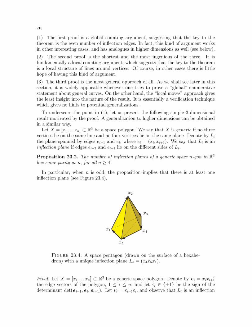
218

(1) The first proof is a global counting argument, suggesting that the key to thetheorem is the even number of inflection edges. In fact, this kind of argument worksin other interesting cases, and has analogues in higher dimensions as well (see below).

(2) The second proof is the shortest and the most ingenious of the three. It isfundamentally a local counting argument, which suggests that the key to the theoremis a local structure of lines around vertices. Of course, in other cases there is littlehope of having this kind of argument.

(3) The third proof is the most general approach of all. As we shall see later in thissection, it is widely applicable whenever one tries to prove a “global” enumerativestatement about general curves. On the other hand, the “local moves” approach givesthe least insight into the nature of the result. It is essentially a verification techniquewhich gives no hints to potential generalizations.

To underscore the point in (1), let us present the following simple 3-dimensionalresult motivated by the proof. A generalization to higher dimensions can be obtainedin a similar way.

Let X = [x1 . . . xn] ⊂ R3 be a space polygon. We say that X is generic if no threevertices lie on the same line and no four vertices lie on the same plane. Denote by Lithe plane spanned by edges ei−1 and ei, where ei = (xi, xi+1). We say that Li is aninflection plane if edges ei−2 and ei+1 lie on the different sides of Li.

Proposition 23.2. The number of inflection planes of a generic space n-gon in R3

has same parity as n, for all n ≥ 4.

In particular, when n is odd, the proposition implies that there is at least oneinflection plane (see Figure 23.4).

x1

x2

x3

x4

x5

Figure 23.4. A space pentagon (drawn on the surface of a hexahe-dron) with a unique inflection plane L5 = (x4x5x1).

Proof. Let X = [x1 . . . xn] ⊂ R3 be a generic space polygon. Denote by e i = −−−→xixi+1

the edge vectors of the polygon, 1 ≤ i ≤ n, and let εi ∈ ±1 be the sign of thedeterminant det(e i−1, e i, e i+1). Let νi = εi−1εi, and observe that Li is an inflection

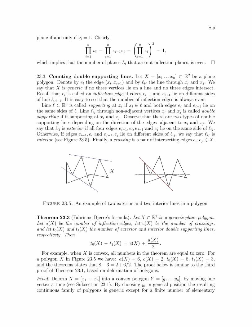
219

plane if and only if νi = 1. Clearly,

n∏

i=1

νi =n∏

i=1

εi−1εi =

(n∏

i=1

εi

)2

= 1,

which implies that the number of planes Li that are not inflection planes, is even.

23.3. Counting double supporting lines. Let X = [x1 . . . xn] ⊂ R2 be a planepolygon. Denote by ei the edge (xi, xi+1) and by ℓij the line through xi and xj . Wesay that X is generic if no three vertices lie on a line and no three edges intersect.Recall that ei is called an inflection edge if edges ei−1 and ei+1 lie on different sidesof line ℓi,i+1. It is easy to see that the number of inflection edges is always even.

Line ℓ ⊂ R2 is called supporting at xi if xi ∈ ℓ and both edges ei and ei+1 lie onthe same sides of ℓ. Line ℓij through non-adjacent vertices xi and xj is called doublesupporting if it supporting at xi and xj . Observe that there are two types of doublesupporting lines depending on the direction of the edges adjacent to xi and xj . Wesay that ℓij is exterior if all four edges ei−1, ei, ej−1 and ej lie on the same side of ℓij .Otherwise, if edges ei−1, ei and ej−1, ej lie on different sides of ℓij , we say that ℓij isinterior (see Figure 23.5). Finally, a crossing is a pair of intersecting edges ei, ej ∈ X.

X

Figure 23.5. An example of two exterior and two interior lines in a polygon.

Theorem 23.3 (Fabricius-Bjerre’s formula). Let X ⊂ R2 be a generic plane polygon.Let a(X) be the number of inflection edges, let c(X) be the number of crossings,and let t0(X) and t1(X) the number of exterior and interior double supporting lines,respectively. Then

t0(X) − t1(X) = c(X) +a(X)

2.

For example, when X is convex, all numbers in the theorem are equal to zero. Fora polygon X in Figure 23.5 we have: a(X) = 6, c(X) = 2, t0(X) = 8, t1(X) = 3,and the theorems states that 8− 3 = 2 + 6/2. The proof below is similar to the thirdproof of Theorem 23.1, based on deformation of polygons.

Proof. Deform X = [x1 . . . xn] into a convex polygon Y = [y1 . . . yn], by moving onevertex a time (see Subsection 23.1). By choosing yi in general position the resultingcontinuous family of polygons is generic except for a finite number of elementary

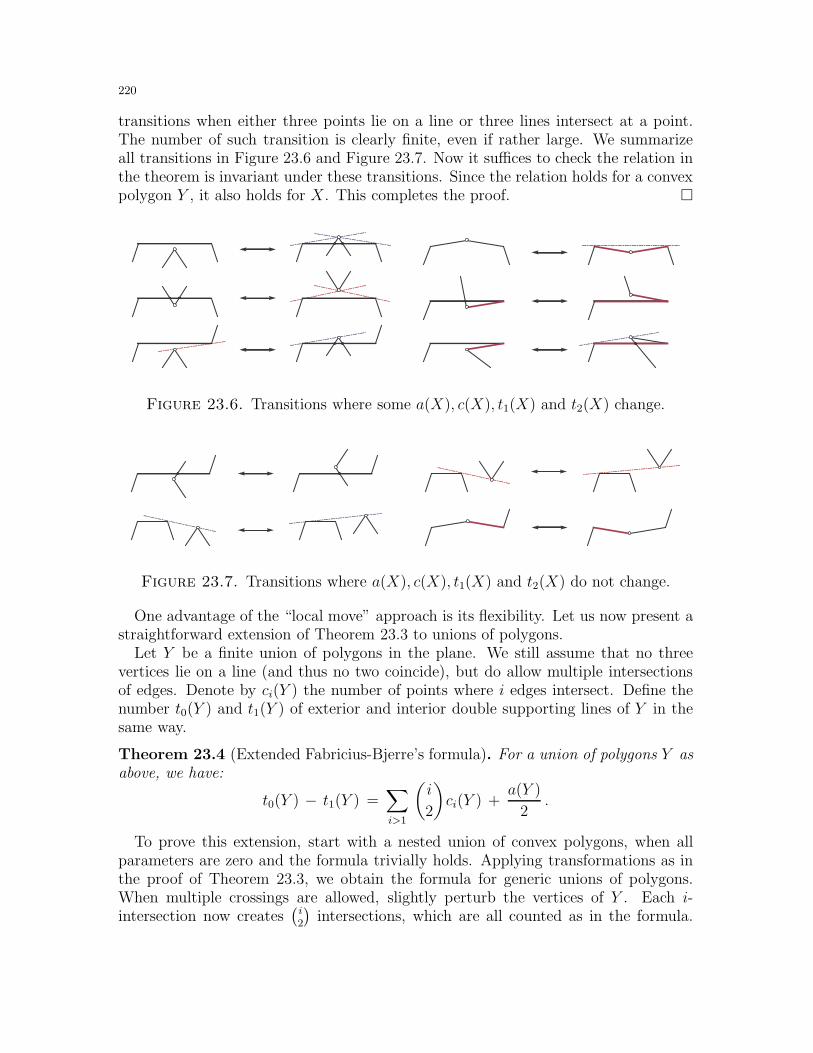
220

transitions when either three points lie on a line or three lines intersect at a point.The number of such transition is clearly finite, even if rather large. We summarizeall transitions in Figure 23.6 and Figure 23.7. Now it suffices to check the relation inthe theorem is invariant under these transitions. Since the relation holds for a convexpolygon Y , it also holds for X. This completes the proof.

Figure 23.6. Transitions where some a(X), c(X), t1(X) and t2(X) change.

Figure 23.7. Transitions where a(X), c(X), t1(X) and t2(X) do not change.

One advantage of the “local move” approach is its flexibility. Let us now present astraightforward extension of Theorem 23.3 to unions of polygons.

Let Y be a finite union of polygons in the plane. We still assume that no threevertices lie on a line (and thus no two coincide), but do allow multiple intersectionsof edges. Denote by ci(Y ) the number of points where i edges intersect. Define thenumber t0(Y ) and t1(Y ) of exterior and interior double supporting lines of Y in thesame way.

Theorem 23.4 (Extended Fabricius-Bjerre’s formula). For a union of polygons Y asabove, we have:

t0(Y ) − t1(Y ) =∑

i>1

(i

2

)ci(Y ) +

a(Y )

2.

To prove this extension, start with a nested union of convex polygons, when allparameters are zero and the formula trivially holds. Applying transformations as inthe proof of Theorem 23.3, we obtain the formula for generic unions of polygons.When multiple crossings are allowed, slightly perturb the vertices of Y . Each i-intersection now creates

(i2

)intersections, which are all counted as in the formula.

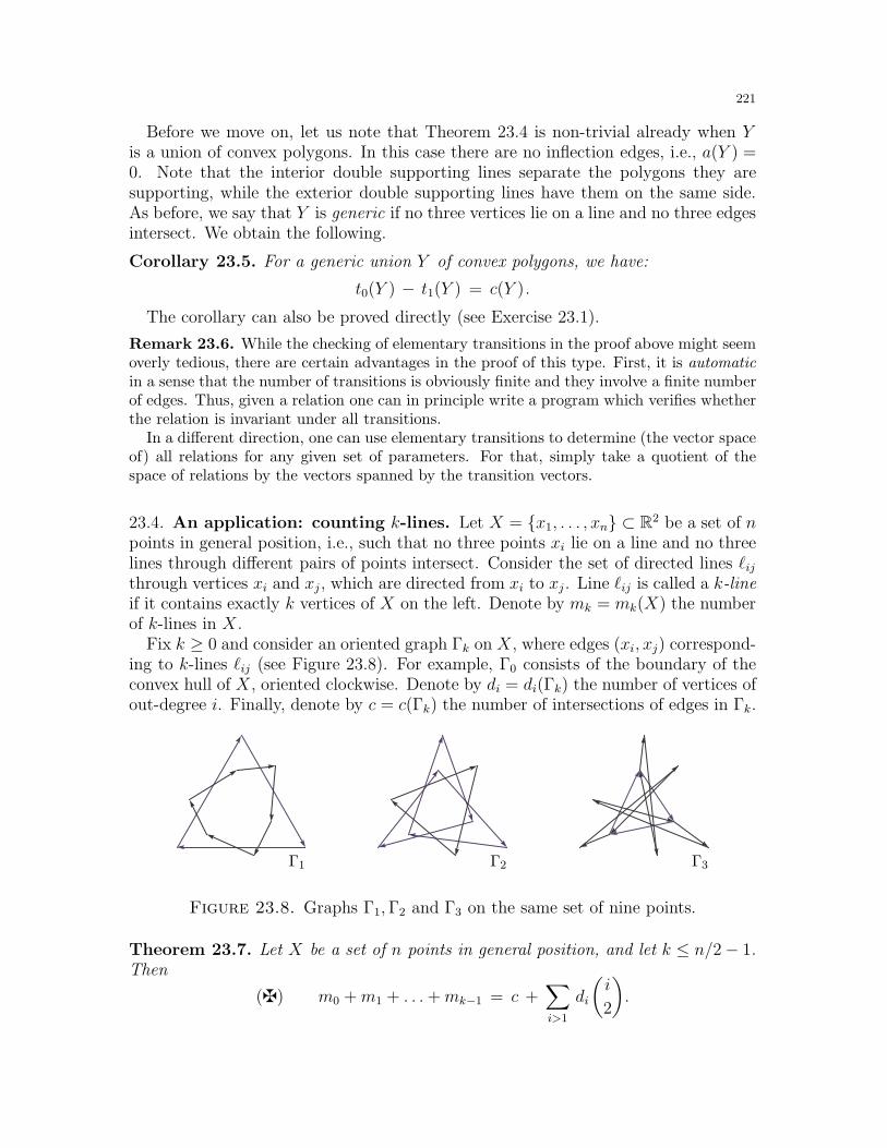
221

Before we move on, let us note that Theorem 23.4 is non-trivial already when Yis a union of convex polygons. In this case there are no inflection edges, i.e., a(Y ) =0. Note that the interior double supporting lines separate the polygons they aresupporting, while the exterior double supporting lines have them on the same side.As before, we say that Y is generic if no three vertices lie on a line and no three edgesintersect. We obtain the following.

Corollary 23.5. For a generic union Y of convex polygons, we have:

t0(Y ) − t1(Y ) = c(Y ).

The corollary can also be proved directly (see Exercise 23.1).

Remark 23.6. While the checking of elementary transitions in the proof above might seemoverly tedious, there are certain advantages in the proof of this type. First, it is automaticin a sense that the number of transitions is obviously finite and they involve a finite numberof edges. Thus, given a relation one can in principle write a program which verifies whetherthe relation is invariant under all transitions.

In a different direction, one can use elementary transitions to determine (the vector spaceof) all relations for any given set of parameters. For that, simply take a quotient of thespace of relations by the vectors spanned by the transition vectors.

23.4. An application: counting k-lines. Let X = x1, . . . , xn ⊂ R2 be a set of npoints in general position, i.e., such that no three points xi lie on a line and no threelines through different pairs of points intersect. Consider the set of directed lines ℓijthrough vertices xi and xj , which are directed from xi to xj . Line ℓij is called a k-lineif it contains exactly k vertices of X on the left. Denote by mk = mk(X) the numberof k-lines in X.

Fix k ≥ 0 and consider an oriented graph Γk on X, where edges (xi, xj) correspond-ing to k-lines ℓij (see Figure 23.8). For example, Γ0 consists of the boundary of theconvex hull of X, oriented clockwise. Denote by di = di(Γk) the number of vertices ofout-degree i. Finally, denote by c = c(Γk) the number of intersections of edges in Γk.

Γ1 Γ2 Γ3

Figure 23.8. Graphs Γ1,Γ2 and Γ3 on the same set of nine points.

Theorem 23.7. Let X be a set of n points in general position, and let k ≤ n/2− 1.Then

(z) m0 +m1 + . . .+mk−1 = c +∑

i>1

di

(i

2

).

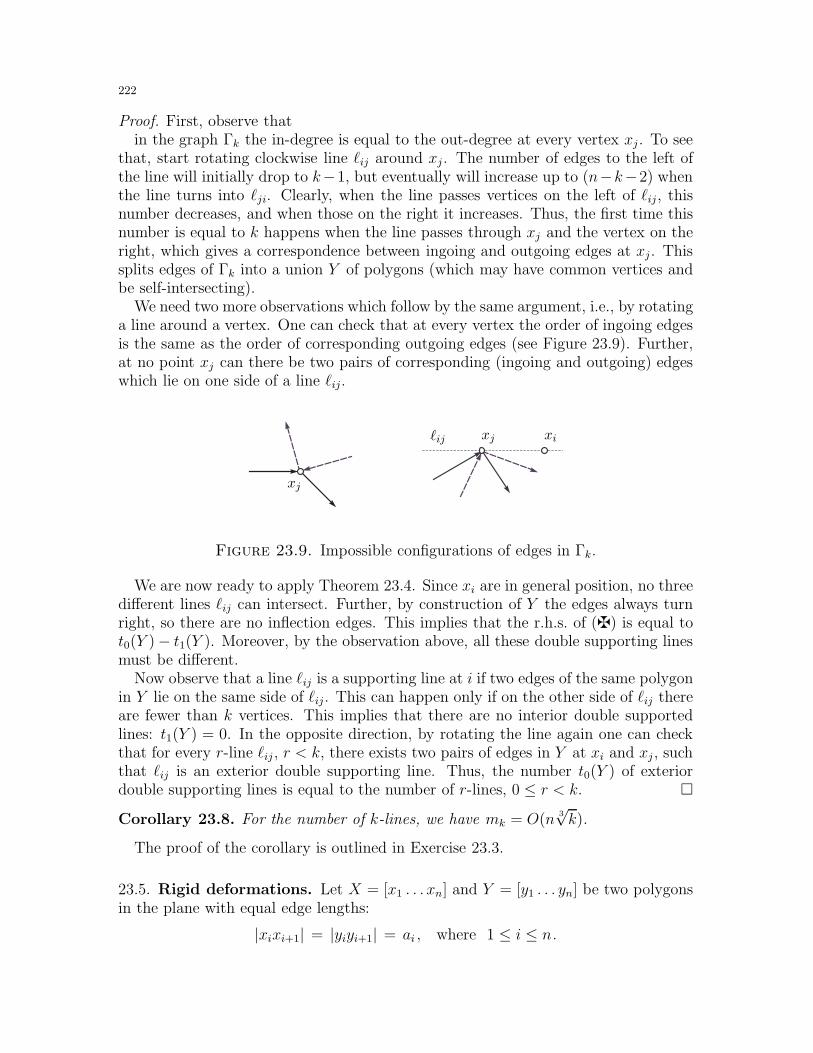
222

Proof. First, observe thatin the graph Γk the in-degree is equal to the out-degree at every vertex xj . To see

that, start rotating clockwise line ℓij around xj . The number of edges to the left ofthe line will initially drop to k−1, but eventually will increase up to (n−k−2) whenthe line turns into ℓji. Clearly, when the line passes vertices on the left of ℓij, thisnumber decreases, and when those on the right it increases. Thus, the first time thisnumber is equal to k happens when the line passes through xj and the vertex on theright, which gives a correspondence between ingoing and outgoing edges at xj . Thissplits edges of Γk into a union Y of polygons (which may have common vertices andbe self-intersecting).

We need two more observations which follow by the same argument, i.e., by rotatinga line around a vertex. One can check that at every vertex the order of ingoing edgesis the same as the order of corresponding outgoing edges (see Figure 23.9). Further,at no point xj can there be two pairs of corresponding (ingoing and outgoing) edgeswhich lie on one side of a line ℓij.

xj

xj

xiℓij

Figure 23.9. Impossible configurations of edges in Γk.

We are now ready to apply Theorem 23.4. Since xi are in general position, no threedifferent lines ℓij can intersect. Further, by construction of Y the edges always turnright, so there are no inflection edges. This implies that the r.h.s. of (z) is equal tot0(Y )− t1(Y ). Moreover, by the observation above, all these double supporting linesmust be different.

Now observe that a line ℓij is a supporting line at i if two edges of the same polygonin Y lie on the same side of ℓij. This can happen only if on the other side of ℓij thereare fewer than k vertices. This implies that there are no interior double supportedlines: t1(Y ) = 0. In the opposite direction, by rotating the line again one can checkthat for every r-line ℓij , r < k, there exists two pairs of edges in Y at xi and xj , suchthat ℓij is an exterior double supporting line. Thus, the number t0(Y ) of exteriordouble supporting lines is equal to the number of r-lines, 0 ≤ r < k.

Corollary 23.8. For the number of k-lines, we have mk = O(n3√k).

The proof of the corollary is outlined in Exercise 23.3.

23.5. Rigid deformations. Let X = [x1 . . . xn] and Y = [y1 . . . yn] be two polygonsin the plane with equal edge lengths:

|xixi+1| = |yiyi+1| = ai , where 1 ≤ i ≤ n.

223

We say that X can be rigidly deformed into Y if there is a continuous family ofpolygonsXt = [x1(t) . . . xn(t)], t ∈ [0, 1], such that |xi(t)xi+1(t)| = ai for all 1 ≤ i ≤ n,and X0 = X, X1 = Y . The family Xt, t ∈ [0, 1] is called a rigid deformation.

Theorem 23.9. Every two polygons with edge lengths (a1, . . . , an) can be rigidlydeformed into each other, unless ai + aj > p/2, ai + ak > p/2, and aj + ak > p/2, forsome i < j < k, where p = a1 + . . .+ an.

The inequalities in the theorem are necessary, since, for example, a polygon inFigure 23.10 cannot be deformed into its inverse. More generally, consider a polygonlinkage L with given edges length (see Section 13), and let ML be its realizationspace. The theorem says that ML is connected unless these inequalities hold. Infact, in the latter case, it is known that the spaceML has two connected componentsseparating polygons and their inverses.

Figure 23.10. A polygon which cannot be deformed into its inverse.

We define a simple rigid deformation to be a rigid deformation Xt, where all Xt

are simple. Clearly, a simple deformation preserves orientation of a polygon. Thefollowing result is the analogue of Theorem 23.9 for simple polygons.

Theorem 23.10 (Carpenter’s rule problem). Every two simple polygons with thesame corresponding edge lengths and the same orientation can be rigidly deformedinto each other by a family of simple polygons.

Just like in the previous two sections, this result can be used to prove a versionof the four vertex theorem (Theorem 21.1) for all equilateral (but not necessarilyconvex) polygons.

Sketch of proof of Corollary 21.19. Denote by N = s− t the difference in the numberof neighboring and disjoint cycles. If we can prove that N = 4 for a specific simplepolygon and that N does not change under the rigid deformation, Theorem 23.10implies the result. Observe that N does not change while the polygon is generic.

Check that we can always deform one simple polygon into another without creatingmore than one degeneracy at a time: line with three vertices or circle with fourvertices. Call a transition through one degeneracy a local move. Going over allpossible local moves as in Figure 23.11, check that s − t is indeed invariant underrigid deformations. It remains to check that N = 4 for a specific polygon.

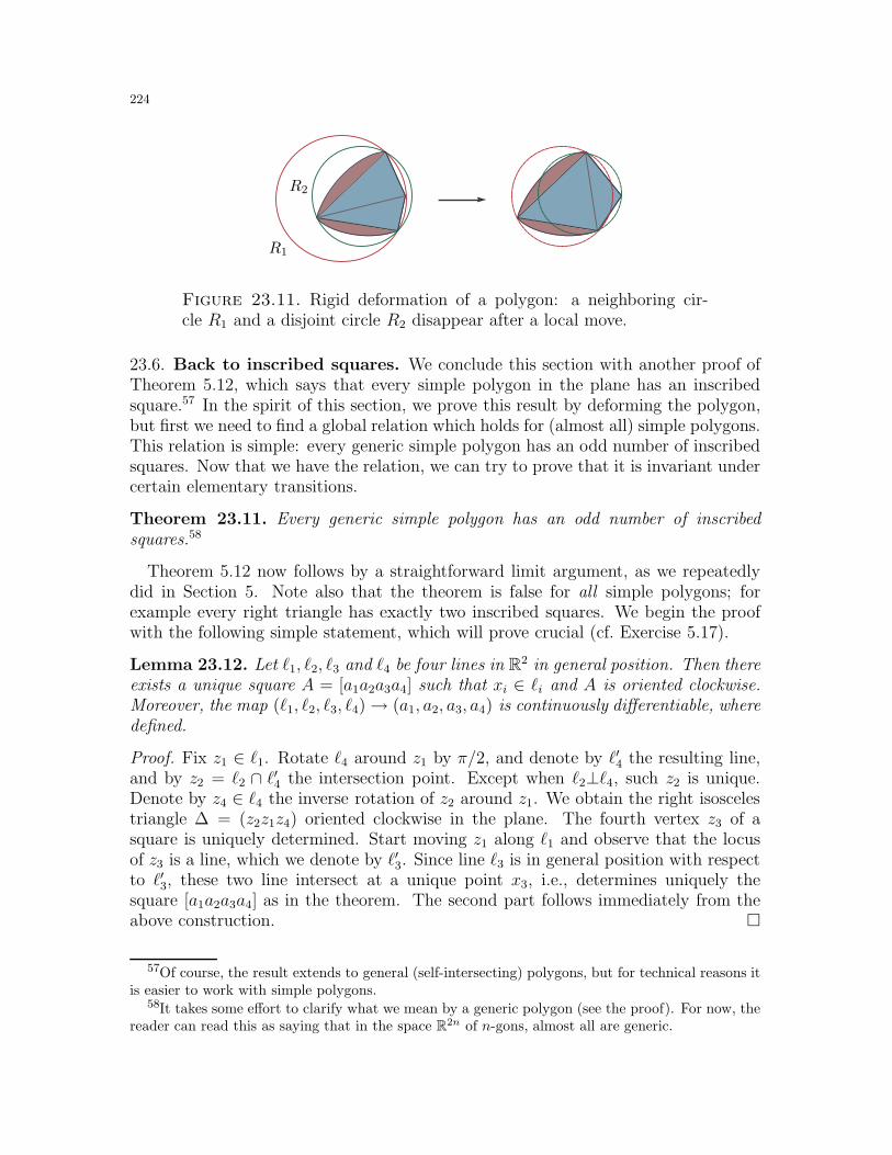
224

R1

R2

Figure 23.11. Rigid deformation of a polygon: a neighboring cir-cle R1 and a disjoint circle R2 disappear after a local move.

23.6. Back to inscribed squares. We conclude this section with another proof ofTheorem 5.12, which says that every simple polygon in the plane has an inscribedsquare.57 In the spirit of this section, we prove this result by deforming the polygon,but first we need to find a global relation which holds for (almost all) simple polygons.This relation is simple: every generic simple polygon has an odd number of inscribedsquares. Now that we have the relation, we can try to prove that it is invariant undercertain elementary transitions.

Theorem 23.11. Every generic simple polygon has an odd number of inscribedsquares.58

Theorem 5.12 now follows by a straightforward limit argument, as we repeatedlydid in Section 5. Note also that the theorem is false for all simple polygons; forexample every right triangle has exactly two inscribed squares. We begin the proofwith the following simple statement, which will prove crucial (cf. Exercise 5.17).

Lemma 23.12. Let ℓ1, ℓ2, ℓ3 and ℓ4 be four lines in R2 in general position. Then thereexists a unique square A = [a1a2a3a4] such that xi ∈ ℓi and A is oriented clockwise.Moreover, the map (ℓ1, ℓ2, ℓ3, ℓ4)→ (a1, a2, a3, a4) is continuously differentiable, wheredefined.

Proof. Fix z1 ∈ ℓ1. Rotate ℓ4 around z1 by π/2, and denote by ℓ′4 the resulting line,and by z2 = ℓ2 ∩ ℓ′4 the intersection point. Except when ℓ2⊥ℓ4, such z2 is unique.Denote by z4 ∈ ℓ4 the inverse rotation of z2 around z1. We obtain the right isoscelestriangle ∆ = (z2z1z4) oriented clockwise in the plane. The fourth vertex z3 of asquare is uniquely determined. Start moving z1 along ℓ1 and observe that the locusof z3 is a line, which we denote by ℓ′3. Since line ℓ3 is in general position with respectto ℓ′3, these two line intersect at a unique point x3, i.e., determines uniquely thesquare [a1a2a3a4] as in the theorem. The second part follows immediately from theabove construction.

57Of course, the result extends to general (self-intersecting) polygons, but for technical reasons itis easier to work with simple polygons.

58It takes some effort to clarify what we mean by a generic polygon (see the proof). For now, thereader can read this as saying that in the space R2n of n-gons, almost all are generic.

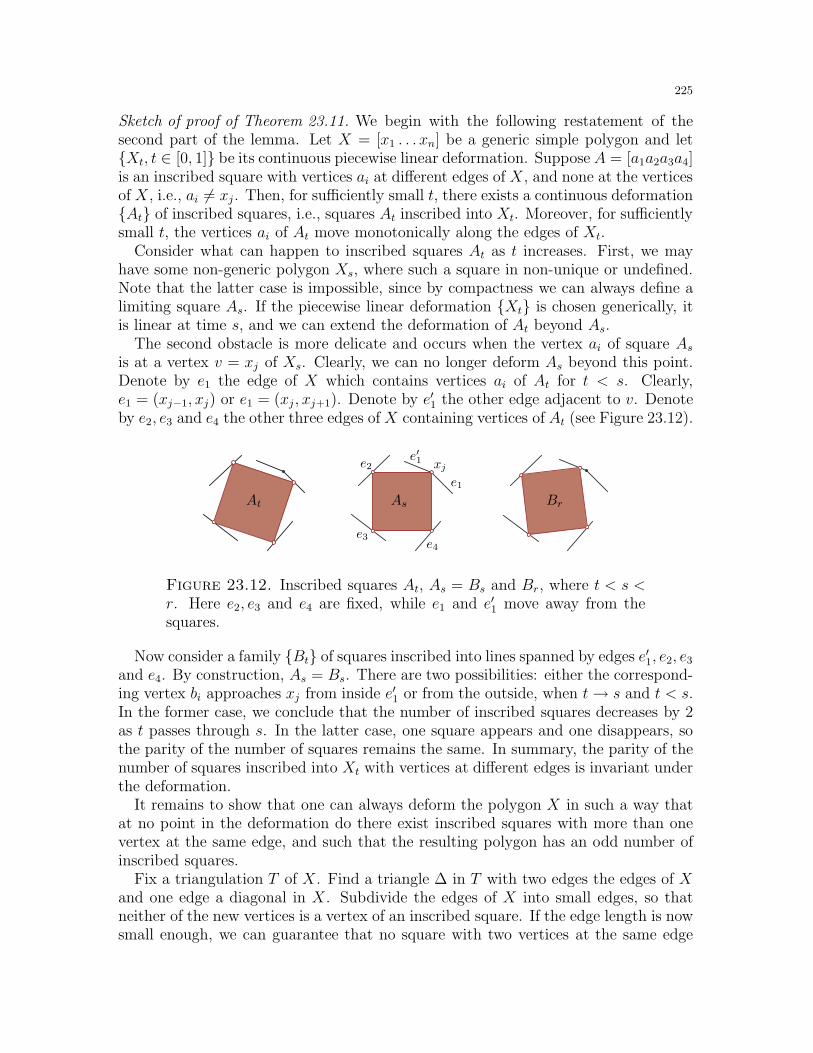
225

Sketch of proof of Theorem 23.11. We begin with the following restatement of thesecond part of the lemma. Let X = [x1 . . . xn] be a generic simple polygon and letXt, t ∈ [0, 1] be its continuous piecewise linear deformation. Suppose A = [a1a2a3a4]is an inscribed square with vertices ai at different edges of X, and none at the verticesof X, i.e., ai 6= xj . Then, for sufficiently small t, there exists a continuous deformationAt of inscribed squares, i.e., squares At inscribed into Xt. Moreover, for sufficientlysmall t, the vertices ai of At move monotonically along the edges of Xt.

Consider what can happen to inscribed squares At as t increases. First, we mayhave some non-generic polygon Xs, where such a square in non-unique or undefined.Note that the latter case is impossible, since by compactness we can always define alimiting square As. If the piecewise linear deformation Xt is chosen generically, itis linear at time s, and we can extend the deformation of At beyond As.

The second obstacle is more delicate and occurs when the vertex ai of square Asis at a vertex v = xj of Xs. Clearly, we can no longer deform As beyond this point.Denote by e1 the edge of X which contains vertices ai of At for t < s. Clearly,e1 = (xj−1, xj) or e1 = (xj , xj+1). Denote by e′1 the other edge adjacent to v. Denoteby e2, e3 and e4 the other three edges of X containing vertices of At (see Figure 23.12).

At As Br

xj

e1

e′1e2

e3e4

Figure 23.12. Inscribed squares At, As = Bs and Br, where t < s <r. Here e2, e3 and e4 are fixed, while e1 and e′1 move away from thesquares.

Now consider a family Bt of squares inscribed into lines spanned by edges e′1, e2, e3and e4. By construction, As = Bs. There are two possibilities: either the correspond-ing vertex bi approaches xj from inside e′1 or from the outside, when t→ s and t < s.In the former case, we conclude that the number of inscribed squares decreases by 2as t passes through s. In the latter case, one square appears and one disappears, sothe parity of the number of squares remains the same. In summary, the parity of thenumber of squares inscribed into Xt with vertices at different edges is invariant underthe deformation.

It remains to show that one can always deform the polygon X in such a way thatat no point in the deformation do there exist inscribed squares with more than onevertex at the same edge, and such that the resulting polygon has an odd number ofinscribed squares.

Fix a triangulation T of X. Find a triangle ∆ in T with two edges the edges of Xand one edge a diagonal in X. Subdivide the edges of X into small edges, so thatneither of the new vertices is a vertex of an inscribed square. If the edge length is nowsmall enough, we can guarantee that no square with two vertices at the same edge

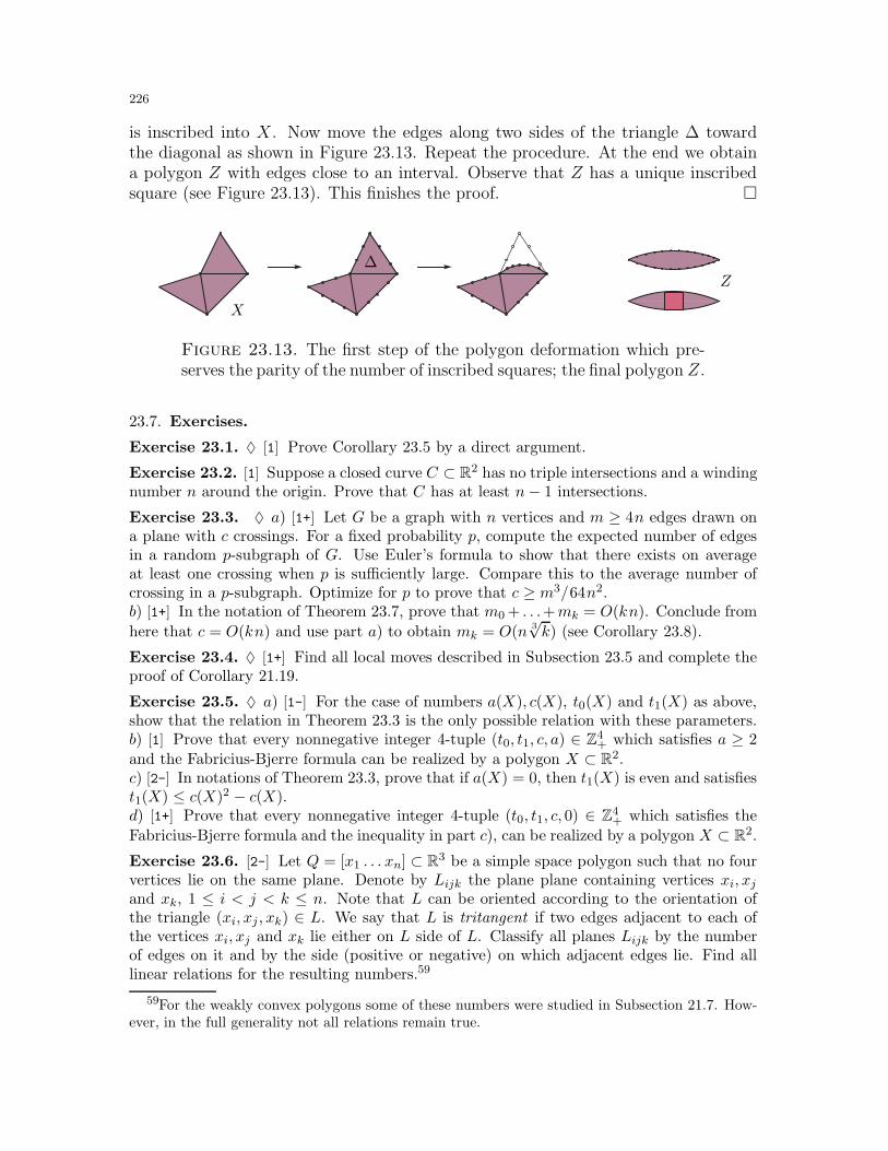
226

is inscribed into X. Now move the edges along two sides of the triangle ∆ towardthe diagonal as shown in Figure 23.13. Repeat the procedure. At the end we obtaina polygon Z with edges close to an interval. Observe that Z has a unique inscribedsquare (see Figure 23.13). This finishes the proof.

X

Z∆

Figure 23.13. The first step of the polygon deformation which pre-serves the parity of the number of inscribed squares; the final polygon Z.

23.7. Exercises.

Exercise 23.1. ♦ [1] Prove Corollary 23.5 by a direct argument.

Exercise 23.2. [1] Suppose a closed curve C ⊂ R2 has no triple intersections and a windingnumber n around the origin. Prove that C has at least n− 1 intersections.

Exercise 23.3. ♦ a) [1+] Let G be a graph with n vertices and m ≥ 4n edges drawn ona plane with c crossings. For a fixed probability p, compute the expected number of edgesin a random p-subgraph of G. Use Euler’s formula to show that there exists on averageat least one crossing when p is sufficiently large. Compare this to the average number ofcrossing in a p-subgraph. Optimize for p to prove that c ≥ m3/64n2.b) [1+] In the notation of Theorem 23.7, prove that m0 + . . .+mk = O(kn). Conclude from

here that c = O(kn) and use part a) to obtain mk = O(n 3√k) (see Corollary 23.8).

Exercise 23.4. ♦ [1+] Find all local moves described in Subsection 23.5 and complete theproof of Corollary 21.19.

Exercise 23.5. ♦ a) [1-] For the case of numbers a(X), c(X), t0(X) and t1(X) as above,show that the relation in Theorem 23.3 is the only possible relation with these parameters.b) [1] Prove that every nonnegative integer 4-tuple (t0, t1, c, a) ∈ Z4

+ which satisfies a ≥ 2and the Fabricius-Bjerre formula can be realized by a polygon X ⊂ R2.c) [2-] In notations of Theorem 23.3, prove that if a(X) = 0, then t1(X) is even and satisfiest1(X) ≤ c(X)2 − c(X).d) [1+] Prove that every nonnegative integer 4-tuple (t0, t1, c, 0) ∈ Z4

+ which satisfies the

Fabricius-Bjerre formula and the inequality in part c), can be realized by a polygon X ⊂ R2.

Exercise 23.6. [2-] Let Q = [x1 . . . xn] ⊂ R3 be a simple space polygon such that no fourvertices lie on the same plane. Denote by Lijk the plane plane containing vertices xi, xjand xk, 1 ≤ i < j < k ≤ n. Note that L can be oriented according to the orientation ofthe triangle (xi, xj , xk) ∈ L. We say that L is tritangent if two edges adjacent to each ofthe vertices xi, xj and xk lie either on L side of L. Classify all planes Lijk by the numberof edges on it and by the side (positive or negative) on which adjacent edges lie. Find alllinear relations for the resulting numbers.59

59For the weakly convex polygons some of these numbers were studied in Subsection 21.7. How-ever, in the full generality not all relations remain true.

227

Exercise 23.7. [2-] Use the stereographic projection to obtain the analogues of results inthe previous exercise for the numbers of neighboring and disjoint circumscribed circles (seeSubsection 21.7).

Exercise 23.8. a) [1+] Find a space polygon in R3 isotopic to the trefoil knot, and withouttritangent planes.b) [2-] Let Q be space polygon in R3 isotopic to the trefoil knot, and such that Q projectsonto a plane with the usual diagram with three crossings. Prove that Q has a tritangentplane.

Exercise 23.9. [2-] Let X = [x1 . . . xn] ⊂ R2 be a polygon with vertices in general position,and let ei = (xi, xi+1) be the edges of X. An interval u = (xi, y), y ∈ X, is called quasi-normal at xi if both angles of u and ei−1, ei are acute or both are obtuse. Define a signε(u) ∈ ±1 of a normal u to be 1 if the angles are acute and −1 if the angles are obtuse.A diagonal (xi, xj) is called a double quasi-normal if it is quasi-normal at both vertices(see Subsection 9.4). It is called positive if ε(xi, xj)ε(xj , xi) = 1; otherwise, it is callednegative. Denote by n+(X) and n−(X) the number of positive and negative double quasi-normals. Define a perpendicular to be an interval u = (xi, y) such that y ∈ ej for some ejand (xi, y)⊥ej . Denote by p+(X) and p−(X) the number of perpendiculars u such thatε(u) = 1 and ε(u) = −1, respectively. Use deformations of polygons to prove that

n+(X) − n−(X) + p+(X) − p−(X) + c(X) = 0,

where c(X) is the number of crossings of X.

Exercise 23.10. Let C ⊂ R2 be an oriented closed piecewise linear curve with n doubleintersections and no triple intersections. A loop is a closed portion of curve without doublepoints.a) [1] Note that C has at most 2n loops. Prove that if C has exactly 2n loops, then betweenevery two points on C corresponding to a double crossing there are exactly n curve arcs.Such curves are called maximally looped.b) [1+] Suppose C has at least n+ 1 loops. Prove that n is odd.c) [1+] Denote by r(C) the sum of (π−αi), over all angles αi on the left of the curve. Provethat r(C) = 2π(n+ − n− ± 1), where n+ and n− is the number of positive and negativedouble points, respectively.d) [1] Use this to prove that if C is maximally looped, then r(C) ∈ −4π, 0, 4π.d) [1] Use part c) of Exercise 23.5 to show that if C is maximally looped and has no inflectionedges, then C has no interior double supporting lines.e) [1-] Use Theorem 23.3 to conclude that every curve C as in part d) has exactly n doublesupporting lines.

Exercise 23.11. [2-] Find a simple unknotted space polygon Q ⊂ R3 which cannot berigidly deformed into a flat convex polygon. In other words, prove that Theorem 23.10does not extend to R3.

Exercise 23.12. [1+] Prove that every two simple polygons in R4, can be rigidly deformedinto each other. In other words, prove that Theorem 23.10 extends to R4.

Exercise 23.13. (Erdos flip problem) [2] Let Q ⊂ R2 be a non-convex polygon and let Cbe the convex hull of Q. Choose edge e of C that is not in Q and reflect the portion of Qacross e, as in Figure 23.14. Repeat such flip transformations until a convex polygon isobtained. Prove that the process stops after finitely many steps.

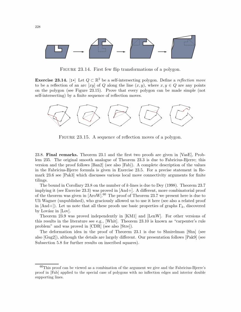
228

Figure 23.14. First few flip transformations of a polygon.

Exercise 23.14. [1+] Let Q ⊂ R2 be a self-intersecting polygon. Define a reflection moveto be a reflection of an arc [xy] of Q along the line (x, y), where x, y ∈ Q are any pointson the polygon (see Figure 23.15). Prove that every polygon can be made simple (notself-intersecting) by a finite sequence of reflection moves.

Figure 23.15. A sequence of reflection moves of a polygon.

23.8. Final remarks. Theorem 23.1 and the first two proofs are given in [VasE], Prob-lem 235. The original smooth analogue of Theorem 23.3 is due to Fabricius-Bjerre; thisversion and the proof follows [Ban2] (see also [Fab]). A complete description of the valuesin the Fabricius-Bjerre formula is given in Exercise 23.5. For a precise statement in Re-mark 23.6 see [Pak3] which discusses various local move connectivity arguments for finitetilings.

The bound in Corollary 23.8 on the number of k-lines is due to Dey (1998). Theorem 23.7implying it (see Exercise 23.3) was proved in [And+]. A different, more combinatorial proofof the theorem was given in [AroW].60 The proof of Theorem 23.7 we present here is due toUli Wagner (unpublished), who graciously allowed us to use it here (see also a related proofin [And+]). Let us note that all these proofs use basic properties of graphs Γk, discoveredby Lovasz in [Lov].

Theorem 23.9 was proved independently in [KM1] and [LenW]. For other versions ofthis results in the literature see e.g., [Whit]. Theorem 23.10 is known as “carpenter’s ruleproblem” and was proved in [CDR] (see also [Stre]).

The deformation idea in the proof of Theorem 23.1 is due to Shnirelman [Shn] (see

also [Gug2]), although the details are largely different. Our presentation follows [Pak9] (see

Subsection 5.8 for further results on inscribed squares).

60This proof can be viewed as a combination of the argument we give and the Fabricius-Bjerre’sproof in [Fab] applied to the special case of polygons with no inflection edges and interior doublesupporting lines.

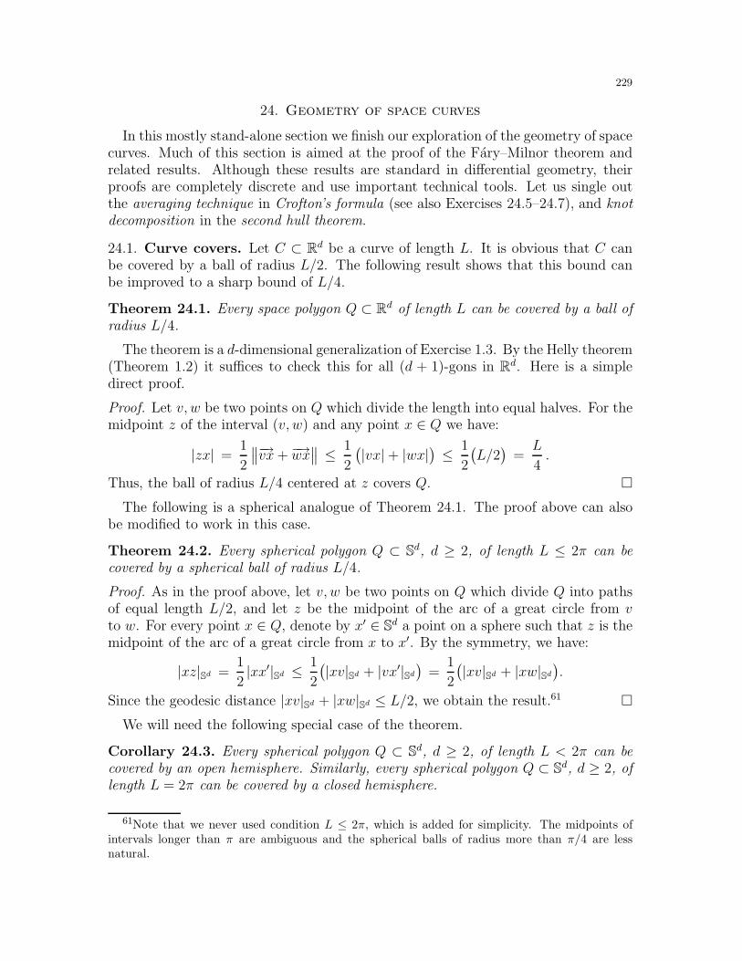
229

24. Geometry of space curves

In this mostly stand-alone section we finish our exploration of the geometry of spacecurves. Much of this section is aimed at the proof of the Fary–Milnor theorem andrelated results. Although these results are standard in differential geometry, theirproofs are completely discrete and use important technical tools. Let us single outthe averaging technique in Crofton’s formula (see also Exercises 24.5–24.7), and knotdecomposition in the second hull theorem.

24.1. Curve covers. Let C ⊂ Rd be a curve of length L. It is obvious that C canbe covered by a ball of radius L/2. The following result shows that this bound canbe improved to a sharp bound of L/4.

Theorem 24.1. Every space polygon Q ⊂ Rd of length L can be covered by a ball ofradius L/4.

The theorem is a d-dimensional generalization of Exercise 1.3. By the Helly theorem(Theorem 1.2) it suffices to check this for all (d + 1)-gons in Rd. Here is a simpledirect proof.

Proof. Let v, w be two points on Q which divide the length into equal halves. For themidpoint z of the interval (v, w) and any point x ∈ Q we have:

|zx| =1

2

∥∥−→vx+−→wx∥∥ ≤ 1

2

(|vx|+ |wx|

)≤ 1

2

(L/2

)=

L

4.

Thus, the ball of radius L/4 centered at z covers Q.

The following is a spherical analogue of Theorem 24.1. The proof above can alsobe modified to work in this case.

Theorem 24.2. Every spherical polygon Q ⊂ Sd, d ≥ 2, of length L ≤ 2π can becovered by a spherical ball of radius L/4.

Proof. As in the proof above, let v, w be two points on Q which divide Q into pathsof equal length L/2, and let z be the midpoint of the arc of a great circle from vto w. For every point x ∈ Q, denote by x′ ∈ Sd a point on a sphere such that z is themidpoint of the arc of a great circle from x to x′. By the symmetry, we have:

|xz|Sd =1

2|xx′|Sd ≤ 1

2

(|xv|Sd + |vx′|Sd

)=

1

2

(|xv|Sd + |xw|Sd

).

Since the geodesic distance |xv|Sd + |xw|Sd ≤ L/2, we obtain the result.61

We will need the following special case of the theorem.

Corollary 24.3. Every spherical polygon Q ⊂ Sd, d ≥ 2, of length L < 2π can becovered by an open hemisphere. Similarly, every spherical polygon Q ⊂ Sd, d ≥ 2, oflength L = 2π can be covered by a closed hemisphere.

61Note that we never used condition L ≤ 2π, which is added for simplicity. The midpoints ofintervals longer than π are ambiguous and the spherical balls of radius more than π/4 are lessnatural.

230

24.2. Total curvature. For a triangle (xyz), the exterior angle η(xyz) at a vertex yis defined as

η(xyz) = π − ∠xyz .

Let Q ⊂ Rd be a simple (non-self-intersecting) space polygon. The total curvatureκ(Q) is the sum of the exterior angles of Q. This definition is robust enough so thatwhen polygons approximate a smooth closed curve C ⊂ Rd, the total curvature ofthe polygons converges to the total curvature of the curve κ(C).

The following beautiful result is the first step in the understanding of total curva-ture.

Theorem 24.4 (Fenchel). For every simple space polygon Q ⊂ R3, the total curvatureκ(Q) ≥ 2π. The equality holds if and only Q is flat and convex.

Proof. Let Q = [v1 . . . vn] ⊂ R3. For every edge vector e1 = (v1v2), . . . , ed−1 =(vn−1vn), en = (vnv1), consider a point on a unit sphere xi ∈ S2 so that (Oxi) isa unit vector along ei. Connect points xi and xi+1 with the shortest path, so thatR = [x1 . . . xn] is a spherical polygon. By definition, the exterior angle η(vi−1vivi+1)of Q is equal to the length |xixi+1|S2 on a sphere. Thus κ(Q) = |R|S2, the length ofthe spherical polygon.

Now observe that R cannot lie in an (open) hemisphere. Indeed, otherwise all edgevectors ei are pointing into the same half-space, and since the sum of ei is equal to O,this is impossible. On the other hand, by Corollary 24.3, any curve on a sphere oflength < 2π can be covered by a hemisphere. Therefore |R|S2 ≥ 2π, which proves thefirst part of the theorem.

For the second part, from above and the second part of Corollary 24.3, the equalitycan occur only when Q lies in a plane. Finally, for the plane convex polygons theresult follows from a direct calculation of the interior angles.

24.3. The Fary–Milnor theorem. In the previous section we proved Fenchel’s the-orem that every curve in R3 has total curvature at least 2π. The main result of thissection is a lower bound of 4π for knotted curves.

We say that a space polygon Q ⊂ R3 is knotted if it is simple and knotted as aclosed curve.

Theorem 24.5 (Fary–Milnor). For every knotted space polygon Q ⊂ R3, the totalcurvature κ(Q) ≥ 4π.

The proof is again based on spherical geometry. Let C ⊂ S2 be a spherical polygonalcurve on a unit sphere. For every point x ∈ S2, denote by nC(x) the number of pointsof intersection of C and a plane Hx orthogonal to (Ox). The values of nC subdividethe sphere into spherical polygons A1, . . . , Ak with constant value νi on Ai. Define

NC =k∑

i=1

νi · area(Ai) =

∫

S2

nC(x) dx .

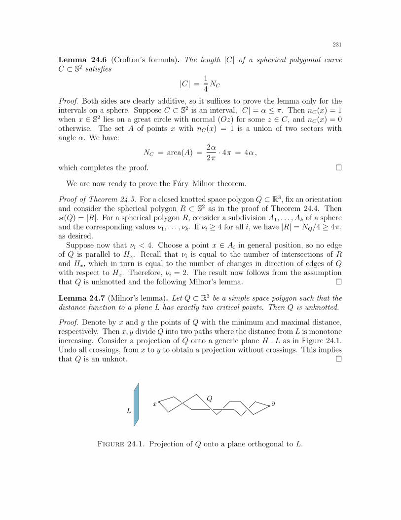
231

Lemma 24.6 (Crofton’s formula). The length |C| of a spherical polygonal curveC ⊂ S2 satisfies

|C| =1

4NC

Proof. Both sides are clearly additive, so it suffices to prove the lemma only for theintervals on a sphere. Suppose C ⊂ S2 is an interval, |C| = α ≤ π. Then nC(x) = 1when x ∈ S2 lies on a great circle with normal (Oz) for some z ∈ C, and nC(x) = 0otherwise. The set A of points x with nC(x) = 1 is a union of two sectors withangle α. We have:

NC = area(A) =2α

2π· 4π = 4α ,

which completes the proof.

We are now ready to prove the Fary–Milnor theorem.

Proof of Theorem 24.5. For a closed knotted space polygonQ ⊂ R3, fix an orientationand consider the spherical polygon R ⊂ S2 as in the proof of Theorem 24.4. Thenκ(Q) = |R|. For a spherical polygon R, consider a subdivision A1, . . . , Ak of a sphereand the corresponding values ν1, . . . , νk. If νi ≥ 4 for all i, we have |R| = NQ/4 ≥ 4π,as desired.

Suppose now that νi < 4. Choose a point x ∈ Ai in general position, so no edgeof Q is parallel to Hx. Recall that νi is equal to the number of intersections of Rand Hx, which in turn is equal to the number of changes in direction of edges of Qwith respect to Hx. Therefore, νi = 2. The result now follows from the assumptionthat Q is unknotted and the following Milnor’s lemma.

Lemma 24.7 (Milnor’s lemma). Let Q ⊂ R3 be a simple space polygon such that thedistance function to a plane L has exactly two critical points. Then Q is unknotted.

Proof. Denote by x and y the points of Q with the minimum and maximal distance,respectively. Then x, y divide Q into two paths where the distance from L is monotoneincreasing. Consider a projection of Q onto a generic plane H⊥L as in Figure 24.1.Undo all crossings, from x to y to obtain a projection without crossings. This impliesthat Q is an unknot.

Q

Lx y

Figure 24.1. Projection of Q onto a plane orthogonal to L.

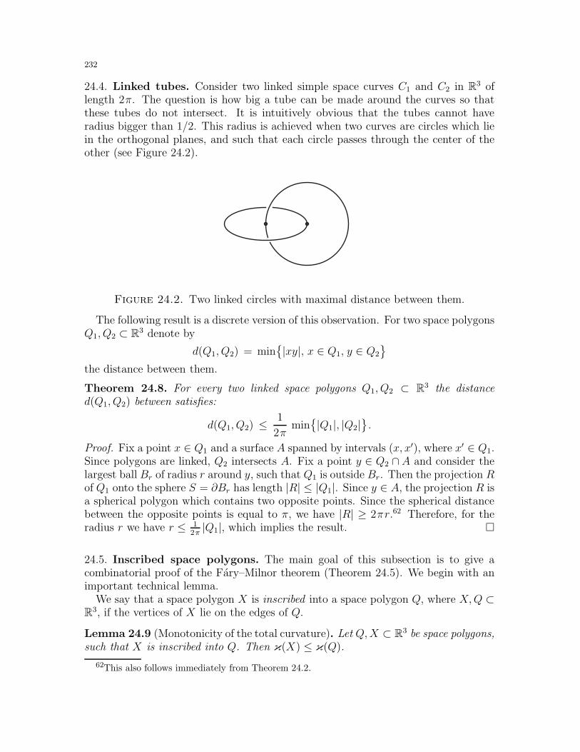
232

24.4. Linked tubes. Consider two linked simple space curves C1 and C2 in R3 oflength 2π. The question is how big a tube can be made around the curves so thatthese tubes do not intersect. It is intuitively obvious that the tubes cannot haveradius bigger than 1/2. This radius is achieved when two curves are circles which liein the orthogonal planes, and such that each circle passes through the center of theother (see Figure 24.2).

Figure 24.2. Two linked circles with maximal distance between them.

The following result is a discrete version of this observation. For two space polygonsQ1, Q2 ⊂ R3 denote by

d(Q1, Q2) = min|xy|, x ∈ Q1, y ∈ Q2

the distance between them.

Theorem 24.8. For every two linked space polygons Q1, Q2 ⊂ R3 the distanced(Q1, Q2) between satisfies:

d(Q1, Q2) ≤1

2πmin

|Q1|, |Q2|

.

Proof. Fix a point x ∈ Q1 and a surface A spanned by intervals (x, x′), where x′ ∈ Q1.Since polygons are linked, Q2 intersects A. Fix a point y ∈ Q2 ∩ A and consider thelargest ball Br of radius r around y, such that Q1 is outside Br. Then the projection Rof Q1 onto the sphere S = ∂Br has length |R| ≤ |Q1|. Since y ∈ A, the projection R isa spherical polygon which contains two opposite points. Since the spherical distancebetween the opposite points is equal to π, we have |R| ≥ 2πr.62 Therefore, for theradius r we have r ≤ 1

2π|Q1|, which implies the result.

24.5. Inscribed space polygons. The main goal of this subsection is to give acombinatorial proof of the Fary–Milnor theorem (Theorem 24.5). We begin with animportant technical lemma.

We say that a space polygon X is inscribed into a space polygon Q, where X,Q ⊂R3, if the vertices of X lie on the edges of Q.

Lemma 24.9 (Monotonicity of the total curvature). Let Q,X ⊂ R3 be space polygons,such that X is inscribed into Q. Then κ(X) ≤ κ(Q).

62This also follows immediately from Theorem 24.2.

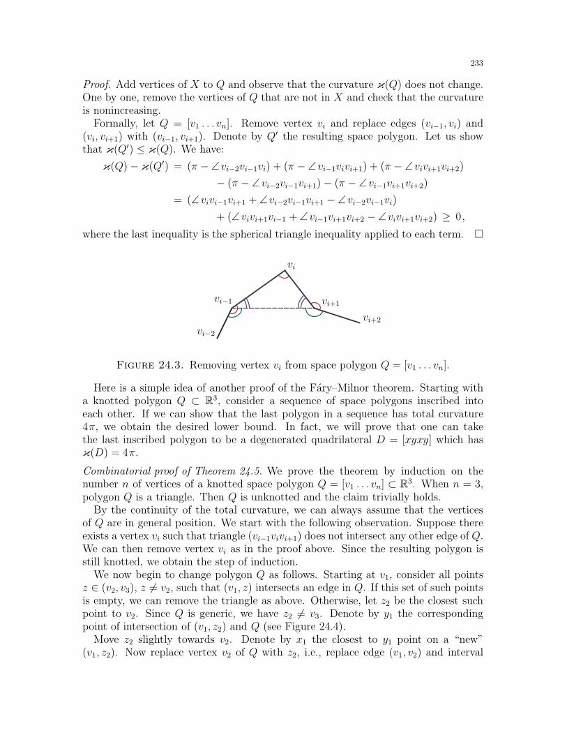
233

Proof. Add vertices of X to Q and observe that the curvature κ(Q) does not change.One by one, remove the vertices of Q that are not in X and check that the curvatureis nonincreasing.

Formally, let Q = [v1 . . . vn]. Remove vertex vi and replace edges (vi−1, vi) and(vi, vi+1) with (vi−1, vi+1). Denote by Q′ the resulting space polygon. Let us showthat κ(Q′) ≤ κ(Q). We have:

κ(Q)− κ(Q′) = (π − ∠vi−2vi−1vi) + (π − ∠vi−1vivi+1) + (π − ∠vivi+1vi+2)

− (π − ∠vi−2vi−1vi+1)− (π − ∠vi−1vi+1vi+2)

= (∠vivi−1vi+1 + ∠vi−2vi−1vi+1 − ∠vi−2vi−1vi)

+ (∠vivi+1vi−1 + ∠vi−1vi+1vi+2 − ∠vivi+1vi+2) ≥ 0,

where the last inequality is the spherical triangle inequality applied to each term.

vi−2

vi−1

vi

vi+1

vi+2

Figure 24.3. Removing vertex vi from space polygon Q = [v1 . . . vn].

Here is a simple idea of another proof of the Fary–Milnor theorem. Starting witha knotted polygon Q ⊂ R3, consider a sequence of space polygons inscribed intoeach other. If we can show that the last polygon in a sequence has total curvature4π, we obtain the desired lower bound. In fact, we will prove that one can takethe last inscribed polygon to be a degenerated quadrilateral D = [xyxy] which hasκ(D) = 4π.

Combinatorial proof of Theorem 24.5. We prove the theorem by induction on thenumber n of vertices of a knotted space polygon Q = [v1 . . . vn] ⊂ R3. When n = 3,polygon Q is a triangle. Then Q is unknotted and the claim trivially holds.

By the continuity of the total curvature, we can always assume that the verticesof Q are in general position. We start with the following observation. Suppose thereexists a vertex vi such that triangle (vi−1vivi+1) does not intersect any other edge of Q.We can then remove vertex vi as in the proof above. Since the resulting polygon isstill knotted, we obtain the step of induction.

We now begin to change polygon Q as follows. Starting at v1, consider all pointsz ∈ (v2, v3), z 6= v2, such that (v1, z) intersects an edge in Q. If this set of such pointsis empty, we can remove the triangle as above. Otherwise, let z2 be the closest suchpoint to v2. Since Q is generic, we have z2 6= v3. Denote by y1 the correspondingpoint of intersection of (v1, z2) and Q (see Figure 24.4).

Move z2 slightly towards v2. Denote by x1 the closest to y1 point on a “new”(v1, z2). Now replace vertex v2 of Q with z2, i.e., replace edge (v1, v2) and interval

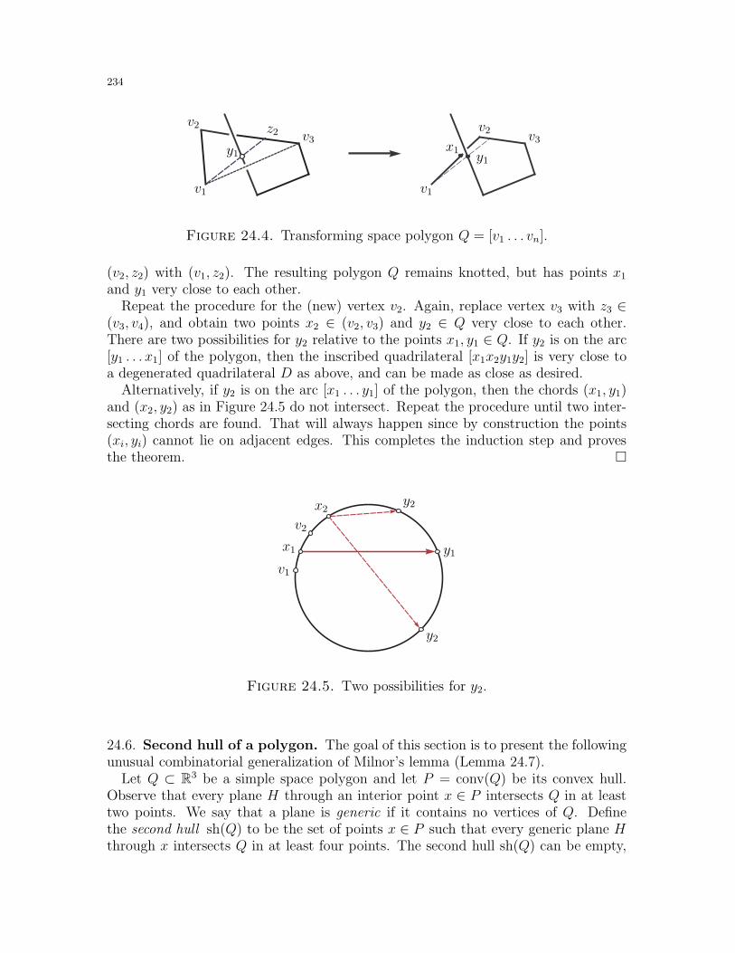
234

v1v1

v2v2

v3v3z2

y1y1

x1

Figure 24.4. Transforming space polygon Q = [v1 . . . vn].

(v2, z2) with (v1, z2). The resulting polygon Q remains knotted, but has points x1

and y1 very close to each other.Repeat the procedure for the (new) vertex v2. Again, replace vertex v3 with z3 ∈

(v3, v4), and obtain two points x2 ∈ (v2, v3) and y2 ∈ Q very close to each other.There are two possibilities for y2 relative to the points x1, y1 ∈ Q. If y2 is on the arc[y1 . . . x1] of the polygon, then the inscribed quadrilateral [x1x2y1y2] is very close toa degenerated quadrilateral D as above, and can be made as close as desired.

Alternatively, if y2 is on the arc [x1 . . . y1] of the polygon, then the chords (x1, y1)and (x2, y2) as in Figure 24.5 do not intersect. Repeat the procedure until two inter-secting chords are found. That will always happen since by construction the points(xi, yi) cannot lie on adjacent edges. This completes the induction step and provesthe theorem.

x1

x2

y1

y2

y2

v1

v2

Figure 24.5. Two possibilities for y2.

24.6. Second hull of a polygon. The goal of this section is to present the followingunusual combinatorial generalization of Milnor’s lemma (Lemma 24.7).

Let Q ⊂ R3 be a simple space polygon and let P = conv(Q) be its convex hull.Observe that every plane H through an interior point x ∈ P intersects Q in at leasttwo points. We say that a plane is generic if it contains no vertices of Q. Definethe second hull sh(Q) to be the set of points x ∈ P such that every generic plane Hthrough x intersects Q in at least four points. The second hull sh(Q) can be empty,

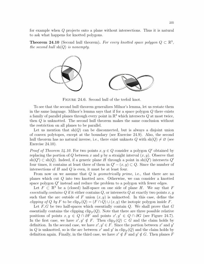
235

for example when Q projects onto a plane without intersections. Thus it is naturalto ask what happens for knotted polygons.

Theorem 24.10 (Second hull theorem). For every knotted space polygon Q ⊂ R3,the second hull sh(Q) is nonempty.

Figure 24.6. Second hull of the trefoil knot.

To see that the second hull theorem generalizes Milnor’s lemma, let us restate themin the same language. Milnor’s lemma says that if for a space polygon Q there existsa family of parallel planes through every point in R3 which intersects Q at most twice,then Q is unknotted. The second hull theorem makes the same conclusion withoutthe restriction on all planes to be parallel.

Let us mention that sh(Q) can be disconnected, but is always a disjoint unionof convex polytopes, except at the boundary (see Exercise 24.9). Also, the secondhull theorem has no natural inverse, i.e., there exist unknots Q with sh(Q) 6= ∅ (seeExercise 24.10).

Proof of Theorem 24.10. For two points x, y ∈ Q consider a polygon Q′ obtained byreplacing the portion of Q between x and y by a straight interval (x, y). Observe thatsh(Q′) ⊂ sh(Q). Indeed, if a generic plane H through a point in sh(Q′) intersects Q′

four times, it contains at least three of them in Q′ − (x, y) ⊂ Q. Since the number ofintersections of H and Q is even, it must be at least four.

From now on we assume that Q is geometrically prime, i.e., that there are noplanes which cut Q into two knotted arcs. Otherwise, we can consider a knottedspace polygon Q′ instead and reduce the problem to a polygon with fewer edges.

Let F ⊂ R3 be a (closed) half-space on one side of plane H . We say that Fessentially contains Q if it either contains Q, or intersects Q at exactly two points x, ysuch that the arc outside of F union (x, y) is unknotted. In this case, define theclipping of Q by F to be clipF (Q) = (F ∩Q) ∪ (x, y) the isotopic polygon inside F .

Let F,G be two half-spaces which essentially contain Q. We shall prove that Gessentially contains the clipping clipF (Q). Note that there are three possible relativepositions of points x, y ∈ Q ∩ ∂F and points x′, y′ ∈ Q ∩ ∂G (see Figure 24.7).In the first case, we have x′, y′ /∈ F . Then clipF (Q) ⊂ G and the claim holds bydefinition. In the second case, we have x′, y′ ∈ F . Since the portion between x′ and y′

in Q is unknotted, so is the arc between x′ and y′ in clipF (Q) and the claim holds bydefinition again. Finally, in the third case, we have x′ /∈ F and y′ /∈ G. Then planes F

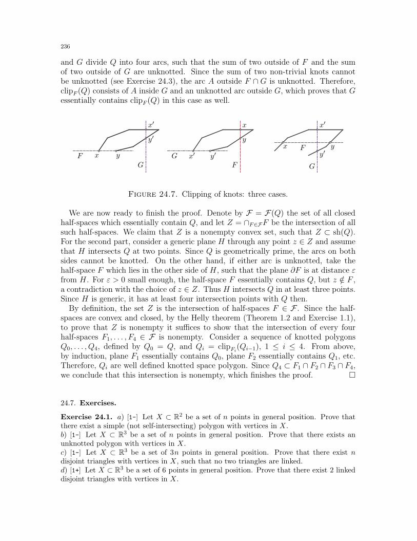
236

and G divide Q into four arcs, such that the sum of two outside of F and the sumof two outside of G are unknotted. Since the sum of two non-trivial knots cannotbe unknotted (see Exercise 24.3), the arc A outside F ∩ G is unknotted. Therefore,clipF (Q) consists of A inside G and an unknotted arc outside G, which proves that Gessentially contains clipF (Q) in this case as well.

x

x

x

x′

x′

x′

yy

y y′y′

y′

F

FF

G

GG

Figure 24.7. Clipping of knots: three cases.

We are now ready to finish the proof. Denote by F = F(Q) the set of all closedhalf-spaces which essentially contain Q, and let Z = ∩F∈FF be the intersection of allsuch half-spaces. We claim that Z is a nonempty convex set, such that Z ⊂ sh(Q).For the second part, consider a generic plane H through any point z ∈ Z and assumethat H intersects Q at two points. Since Q is geometrically prime, the arcs on bothsides cannot be knotted. On the other hand, if either arc is unknotted, take thehalf-space F which lies in the other side of H , such that the plane ∂F is at distance εfrom H . For ε > 0 small enough, the half-space F essentially contains Q, but z /∈ F ,a contradiction with the choice of z ∈ Z. Thus H intersects Q in at least three points.Since H is generic, it has at least four intersection points with Q then.

By definition, the set Z is the intersection of half-spaces F ∈ F . Since the half-spaces are convex and closed, by the Helly theorem (Theorem 1.2 and Exercise 1.1),to prove that Z is nonempty it suffices to show that the intersection of every fourhalf-spaces F1, . . . , F4 ∈ F is nonempty. Consider a sequence of knotted polygonsQ0, . . . , Q4, defined by Q0 = Q, and Qi = clipFi

(Qi−1), 1 ≤ i ≤ 4. From above,by induction, plane F1 essentially contains Q0, plane F2 essentially contains Q1, etc.Therefore, Qi are well defined knotted space polygon. Since Q4 ⊂ F1 ∩ F2 ∩ F3 ∩ F4,we conclude that this intersection is nonempty, which finishes the proof.

24.7. Exercises.

Exercise 24.1. a) [1-] Let X ⊂ R2 be a set of n points in general position. Prove thatthere exist a simple (not self-intersecting) polygon with vertices in X.b) [1-] Let X ⊂ R3 be a set of n points in general position. Prove that there exists anunknotted polygon with vertices in X.c) [1-] Let X ⊂ R3 be a set of 3n points in general position. Prove that there exist ndisjoint triangles with vertices in X, such that no two triangles are linked.d) [1+] Let X ⊂ R3 be a set of 6 points in general position. Prove that there exist 2 linkeddisjoint triangles with vertices in X.

237

Exercise 24.2. (Local convexity of polygons) ♦ [1] Prove that every simple polygonQ ⊂ R2

with interior angles < π is convex. Prove a spherical analogue.

Exercise 24.3. (Sum of knots) [2-] Prove that the sum of two non-trivial knots cannot bean unknot.

Exercise 24.4. (Borsuk) [1] Generalize Fenchel’s Theorem 24.4 to curves in Rd.

Exercise 24.5. (Crofton’s formula for surfaces) ♦ [1] Let S ⊂ R3 be a non-convex 2-dimensional polyhedral surface with the set of vertices V = v1, . . . , vn. Define the totalabsolute curvature κ(S) =

∑i |ωi| the sum of absolute values of curvatures ωi = ω(vi) of

vertices (see Section 25). Generalize Crofton’s formula (Lemma 24.6) to show that κ(S) is2π times the average number of critical points of linear functions on S.

Exercise 24.6. (Buffon’s needle) ♦ Consider an infinite family L of horizontal lines in theplane which stand apart at distance 1 from each other. Let C be a rectifiable curve in R2.Denote by N(C) the number of intersections of C and lines in L. Define ρ = ρ(α, b) to be arigid motion of a plane obtained as a rotation by angle α and then a translation by vector b.Denote by B an axis parallel unit square. Finally, let

N(C) = E[N(ρC)

],

where ρ = ρ(α, b), α ∈ [0, 2π] is a random angle, and b ∈ B is a random vector. Heuristically,think of N(C) as the average number of intersections of C and a random rigid motion of C.a) [1] Prove that the average N(C) is invariant under rigid motions. Prove that N(C) isadditive when a union of two curves is taken. Check that N(C) is continuous as curve C isdeformed.b) [1-] Observe that N(C) = 2 when C is a circle of diameter 1. Conclude from here thatN(C) = 1/π when C is a unit interval.63 More generally, prove that N(C) = |C|/π forevery C.c) [1-] Observe that N(C) = 2 when C is a curve of constant width 1 (see Exercise 3.6).Conclude that |C| = π.

Exercise 24.7. (Random intersections) Let R be the set of rigid motions ρ(α, b) as above.Define the kinematic density dρ = | sinα|dα∧db. For two convex sets X,Y ⊂ R2, denote byN(X,Y ) the number of points in the intersection ∂X∩∂Y . Fix a convex set X and let mi bethe measure of the set of ρ ∈ A such that N(X, ρX) = i. Finally, denote ℓ = perimeter(X)and a = area(X).a) [2-] Prove that

ℓ2 − 4πa = m4 + 2m6 + 3m8 + . . .

Conclude from here the isoperimetric inequality in the plane (Theorem 7.1).b) [1] Consider a subset A(X) ⊂ R of rigid motions ρ(α, b) such that N(X, ρX) ≥ 4. Usepart a) to show that if X is a convex set not equal to a circle, then the subset A(X) haspositive kinematic measure.c) [1] Give an independent proof of part b) using Lemma 9.6.

Exercise 24.8. (Wienholtz ) a) [1+] Prove that every polygon Q ⊂ R2 of length |Q| has aprojection onto a line of length at most |Q|/π.b) [2-] Prove that every space polygon Q ⊂ R3 of length |Q| has a projection onto a planewhich has diameter |Q|/π.

63This result, well known under the name Buffon’s needle, gives a Monte Carlo method for ap-proximating the number π.

238

c) [2] Prove that every space polygon Q ⊂ R3 of length |Q| has a projection onto a planewhich lies in a circle or diameter |Q|/π.

Exercise 24.9. ♦ a) [1] Prove that the closure of every connected component of sh(Q) isa convex polytope.b) [1-] Let L ⊂ R3 be a disjoint union of space polygons which form a nontrivial link.Extend the definition of the second hull to links. Prove that sh(L) 6= ∅.

Exercise 24.10. ♦ a) [1-] Find a simple space polygon in R3 with a disjoint second hull.b) [1-] Find an unknotted space polygon in R3 with a nonempty second hull.c) [1] Find an unknotted space polygon in R3 such that its second hull contains a unit ball.

Exercise 24.11. [2+] In the conditions of the second hull theorem (Theorem 24.10), provethat the closure of sh(Q) intersects Q.

Exercise 24.12. [2] Let L be a link with n components such that every two of themare linked. Prove that there exists a point x ∈ conv(L) such that every plane through xintersects at least n/2 components of L.

Exercise 24.13. (Alexandrov) [1+] Let C be a polygonal curve in R2 with endpoints x, y.Define the total curvature κ = κ(C) to be the sum of exterior angles in the vertices of C.Suppose κ(C) < π. Prove that

|C| ≤ |xy|cosκ

,

and the equality holds only when C has two edges of equal length and angle (π−κ) betweenthem. Extend the result to Rd.

Exercise 24.14. ♦ a) [1+] Let C be a polygonal curve in R2 with endpoints x, y. SupposeCdoes not contain the origin O. Define the visibility angle ϕ(C) to be the length of a projectionof C onto a unit circle centered at O. Denote by α, β the angles between (Ox), (Oy) and C.Prove that

(∗) ϕ(C) ≤ κ(C) + π − α − β .

b) [1+] Prove the analogue of a) for paths in R3. Formally, let C be a polygonal curve in R3

with endpoints x, y, and such that O /∈ C. Let ϕ(C) be the length of a projection of C ontoa unit sphere centered at O, and let α, β be the angles between (Ox), (Oy) and C. Provethat (∗) holds. Conclude that ϕ(Q) ≤ κ(Q) for every (closed, simple) space polygon.c) [1] Use the second hull theorem (Theorem 24.10) to prove that for every knotted spacepolygon Q ⊂ R3 there exists a translation Q′ of Q such that ϕ(Q′) ≥ 4π. Use part b) toobtain the Fary–Milnor theorem (Theorem 24.5).

Exercise 24.15. [1+] Let Q ⊂ R3 be a knotted space polygon. Prove that there exist threedistinct points x, y, z ∈ Q such that y is a midpoint of (x, z).

Exercise 24.16. (Quadrisecants of knots) Let Q ⊂ R3 be a knotted space polygon.a) [1-] Prove that every point in Q lies on a line which intersects Q in at least two otherpoints.b) [2] Prove that there exists a line which intersects Q in at least four points lying ondifferent edges. Such quadruples of points are called quadrisecants.c) [2+] Prove that there there exists a quadrisecant with the order of points on a linealternating with the order of points on Q. These are called alternating quadrisecants.Conclude from here the Fary–Milnor theorem (Theorem 24.5).

239

Exercise 24.17. (Fary theorem and generalizations) a) [1+] Let C ⊂ Br be a general(possibly non-convex and self-intersecting) polygon in the plane, where Br is a disk ofradius r > 0. Denote by |C| the length of C and by κ(C) the total curvature of C. Provethat |C| < rκ(C).b) [2-] Let C ⊂ Br be a polygon in Rd, where Br is a ball of radius r > 0. As before,let κ(C) be the total curvature of C. Prove that |C| < rκ(C).c) [2] Let C,Q ⊂ R2 be two polygons in the plane such that Q is convex and C is inside Q.Prove that the average total curvature is nonincreasing:

κ(C)

|C| ≥κ(Q)

|Q| .

Moreover, the equality holds only when C is a multiple of Q.

Exercise 24.18. Let S1, S2 ⊂ Rd be two PL-homeomorphic PL-surfaces. Define the Frechetdistance

distF (C1, C2) = infφ

maxx∈C1

|xφ(x)|,

where the infimum is over all piecewise linear homeomorphisms φ : S1 → S2.a) [1+] Let C1, C2 ⊂ R2 be two convex polygons in the plane. Prove that

|C1| − |C2| ≤ 2π distF (C1, C2).

b) [2-] Let C1, C2 ⊂ R2 be two simple polygons in the plane. Prove that

|C1| − |C2| ≤[κ(C1) + κ(C2)− 2π

]distF (C1, C2).

c) [2] Let C1, C2 ⊂ R3 be two simple space polygons. Prove that

|C1| − |C2| ≤ π[κ(C1) + κ(C2)− 2π

]distF (C1, C2).

d) [1-] Check that part a) of Exercise 24.17 follows from here, while part b) does not.

Exercise 24.19. (Curvature of graphs in R3) For a graph G denote by G the graph onthe same set of vertices, and with twice as many edges between every two vertices. For an

embedding γ : G→ Γ, where Γ ⊂ R3, and an Eulerian circuit C in G, define

κC(Γ) =1

2κ(γ(C)

).

This notion is called the net total curvature of Γ.a) [2-] Find the analogue of Crofton’s formula (Lemma 24.6) for the net total curvatureb) [1+] Define the Kotzig transformation on Eulerian circuits by changing the direction ona closed segment of a circuit. Prove that every two Eulerian circuits C1, C2 in G can beobtained from each other by a finite sequence of Kotzig transformations.c) [1+] Use parts a) and b) to prove that the net total curvature is independent of theEulerian circuit.

Exercise 24.20. Let Γ ⊂ R3 be a union of three non-intersecting space polygonal curvesbetween two points x, y. Let κ(Γ) be the sum of all exterior angles between pairs of adjacentedges, where the exterior angles in x and y are weighted with 1/2.a) [1] Check that κ(Γ) is equal to the net total curvature of Γ.b) [1+] Prove that κ(Γ) ≥ 3π.c) [2-] Let G be a graph with two vertices and three edges between them, and let Γ be anembedding of G in R3. Prove that if κ(Γ) < 4π, then the Γ is unknotted.

240

Exercise 24.21. a) [2-] Prove that the total length of a net (of inextensible strings) whichholds a sphere is at least 3π.64

b) [1] Show that the bound in a) is tight.c) [2] Suppose a net holds a sphere even if any k links are broken. Prove that the totallength of such net is at least (2k + 3)π.

24.8. Final remarks. Theorem 24.1 goes back to Segre (1937) and was subsequently redis-covered several times. This proof is given in [ChaK]. Theorem 24.4 was proved by Fenchelin 1929, and was extended by Borsuk in 1947 (see Exercise 24.4). A continuous version ofthe proof above was given by Liebmann and later rediscovered by Horn (see [Horn] for asimple proof and references).

We refer to [Ada2, Sos] for an accessible introduction to knot theory. Theorem 24.5 wasdiscovered independently by Fary and Milnor. In our proof we follow the sketch in [Cher],which is close to the original proof in [Mil1]. The linked tube problem in Subsection 24.4was proposed by F. Gehring in 1973. The proof we present is due to M. Ortel [Can+] (seealso [EdeS]). We refer to [Can+] for various extensions and further references.

The combinatorial proof of the Fary–Milnor theorem presented in Subsection 24.5 is dueto Alexander and Bishop [ABi]. They give additional arguments extending the result togeneral curves and making the inequality in the theorem strict. The result on alternatingquadrisecants in the Exercise 24.16 is due to Denne [Den] and can be viewed as yet anotherproof of the Fary–Milnor theorem.

The second hull theorem (Theorem 24.10) is proved in [CKKS], where various extensions

and applications are also presented. These include the extension to nontrivial links (see

Exercise 24.9) and another connection to the Fary–Milnor theorem (see Exercise 24.14).

64The precise definition is a non-trivial part of the exercise. For a simple example of a net whichholds a sphere, take vertices of an equilateral tetrahedron inscribed into S2 and connect them by

geodesics. The total length of these geodesics is equal to 12 arcsin√

2

3≈ 3.65π.

241

25. Geometry of convex polyhedra: basic results

We begin the study of polyhedral surfaces with two most basic results: Euler’sformula and the Gauss–Bonnet theorem. We use bits and pieces of spherical geometryand apply the results to closed geodesics on convex polyhedra (see Section 10).

25.1. Euler’s formula. Let P ⊂ R3 be a convex polytope, and let V,E,F denotethe set of vertices, edges, and faces of P , respectively. The classical Euler’s formulain this case is the following result.

Theorem 25.1 (Euler’s formula). |V | − |E| + |F| = 2.

Even though there is a straightforward inductive proof, the spherical geometryproof below will be a helpful introduction to the method. Note also that in Section 8we already proved the much more general Dehn-Sommerville equations for all simplepolytopes (Theorem 8.1).

Proof. Move P so that it contains the origin O and consider the unit sphere S2 ⊂ R3

with the center at O. Consider a radial projection of the surface ∂P onto S2. In otherwords, for every edge (v, w) ∈ E draw an intersection of S2 and a (planar) cone over(v, w) starting from O. This gives an arc (v′, w′) ⊂ S2 of a great circle. Clearly, everyk-gonal face in P becomes a spherical k-gon.

Let F ∈ F be an i-gonal face of the polytope, let F ′ denotes the correspondingspherical i-gon, and let α(F ′) be the sum of the angles of F ′. By Girard’s formula forpolygons (see Theorem 41.2) we have:

α(F ′) = area(F ′) + (i− 2)π .

Denote by fi the number of i-gonal faces in F and sum the above equation over allfaces F ∈ F . Since the sum of the angles on a sphere in the vertex image v′ is 2π,for all v ∈ V , we have:

2π · |V | = area(S2) +∑

i

fi · (i− 2)π = 4π − 2π · |F| + π ·∑

i

i fi .

On the other hand,∑

i i fi = 2 |E|, since every edge belongs to exactly two faces.Substituting this into above equation gives Euler’s formula.

Of course, Euler’s formula holds in much greater generality, e.g., for all planarmaps, or in higher dimensions (see Section 8). Here is a simple corollary which willprove useful.

Corollary 25.2. Every simplicial polytope with n vertices has 3n−6 edges and 2n−4faces. More generally, this holds for every triangulated surface homeomorphic to asphere S2.

Proof. Suppose P has k faces. Then the number of edges is 32k, and by Euler’s formula

k − 32k + n = 2. Solving this for k gives the result.

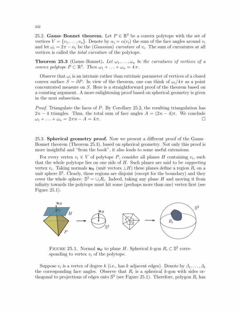
242

25.2. Gauss–Bonnet theorem. Let P ∈ R3 be a convex polytope with the set ofvertices V = v1, . . . , vn. Denote by αi = α(vi) the sum of the face angles around viand let ωi = 2π − αi be the (Gaussian) curvature of vi. The sum of curvatures at allvertices is called the total curvature of the polytope.

Theorem 25.3 (Gauss–Bonnet). Let ω1, . . . , ωn be the curvatures of vertices of aconvex polytope P ⊂ R3. Then ω1 + . . .+ ωn = 4π.

Observe that ωi is an intrinsic rather than extrinsic parameter of vertices of a closedconvex surface S = ∂P . In view of the theorem, one can think of ωi/4π as a pointconcentrated measure on S. Here is a straightforward proof of the theorem based ona counting argument. A more enlightening proof based on spherical geometry is givenin the next subsection.

Proof. Triangulate the faces of P . By Corollary 25.2, the resulting triangulation has2n − 4 triangles. Thus, the total sum of face angles A = (2n − 4)π. We concludeω1 + . . .+ ωn = 2πn− A = 4π.

25.3. Spherical geometry proof. Now we present a different proof of the Gauss–Bonnet theorem (Theorem 25.3), based on spherical geometry. Not only this proof ismore insightful and “from the book”, it also leads to some useful extensions.

For every vertex vi ∈ V of polytope P , consider all planes H containing vi, suchthat the whole polytope lies on one side of H . Such planes are said to be supportingvertex vi. Taking normals uH (unit vectors ⊥H) these planes define a region Ri on aunit sphere S2. Clearly, these regions are disjoint (except for the boundary) and theycover the whole sphere: S2 = ∪iRi. Indeed, taking any plane H and moving it frominfinity towards the polytope must hit some (perhaps more than one) vertex first (seeFigure 25.1).

S2

S2

P

H

vi

vi uH

uH

Ri

Figure 25.1. Normal uH to plane H . Spherical k-gon Ri ⊂ S2 corre-sponding to vertex vi of the polytope.

Suppose vi is a vertex of degree k (i.e., has k adjacent edges). Denote by β1, . . . , βkthe corresponding face angles. Observe that Ri is a spherical k-gon with sides or-thogonal to projections of edges onto S2 (see Figure 25.1). Therefore, polygon Ri has

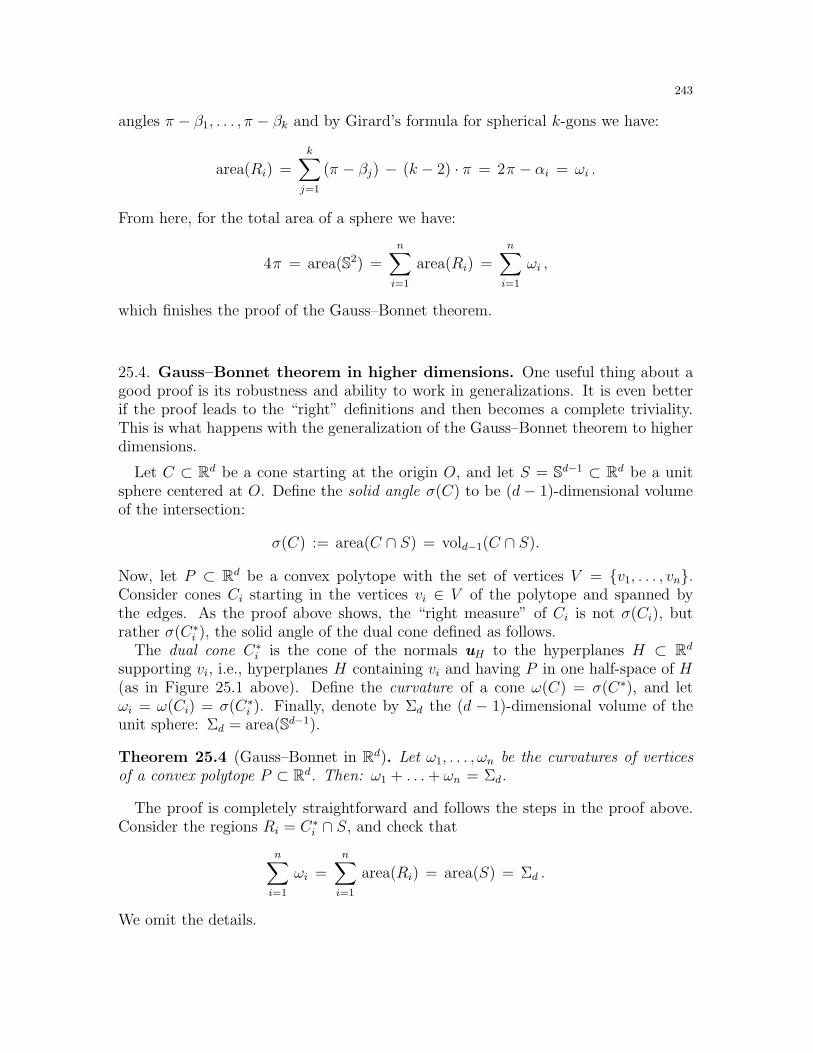
243

angles π − β1, . . . , π − βk and by Girard’s formula for spherical k-gons we have:

area(Ri) =

k∑

j=1

(π − βj) − (k − 2) · π = 2π − αi = ωi .

From here, for the total area of a sphere we have:

4π = area(S2) =n∑

i=1

area(Ri) =n∑

i=1

ωi ,

which finishes the proof of the Gauss–Bonnet theorem.

25.4. Gauss–Bonnet theorem in higher dimensions. One useful thing about agood proof is its robustness and ability to work in generalizations. It is even betterif the proof leads to the “right” definitions and then becomes a complete triviality.This is what happens with the generalization of the Gauss–Bonnet theorem to higherdimensions.

Let C ⊂ Rd be a cone starting at the origin O, and let S = Sd−1 ⊂ Rd be a unitsphere centered at O. Define the solid angle σ(C) to be (d− 1)-dimensional volumeof the intersection:

σ(C) := area(C ∩ S) = vold−1(C ∩ S).

Now, let P ⊂ Rd be a convex polytope with the set of vertices V = v1, . . . , vn.Consider cones Ci starting in the vertices vi ∈ V of the polytope and spanned bythe edges. As the proof above shows, the “right measure” of Ci is not σ(Ci), butrather σ(C∗

i ), the solid angle of the dual cone defined as follows.The dual cone C∗

i is the cone of the normals uH to the hyperplanes H ⊂ Rd

supporting vi, i.e., hyperplanes H containing vi and having P in one half-space of H(as in Figure 25.1 above). Define the curvature of a cone ω(C) = σ(C∗), and letωi = ω(Ci) = σ(C∗

i ). Finally, denote by Σd the (d − 1)-dimensional volume of theunit sphere: Σd = area(Sd−1).

Theorem 25.4 (Gauss–Bonnet in Rd). Let ω1, . . . , ωn be the curvatures of verticesof a convex polytope P ⊂ Rd. Then: ω1 + . . .+ ωn = Σd.

The proof is completely straightforward and follows the steps in the proof above.Consider the regions Ri = C∗

i ∩ S, and check that

n∑

i=1

ωi =

n∑

i=1

area(Ri) = area(S) = Σd .

We omit the details.

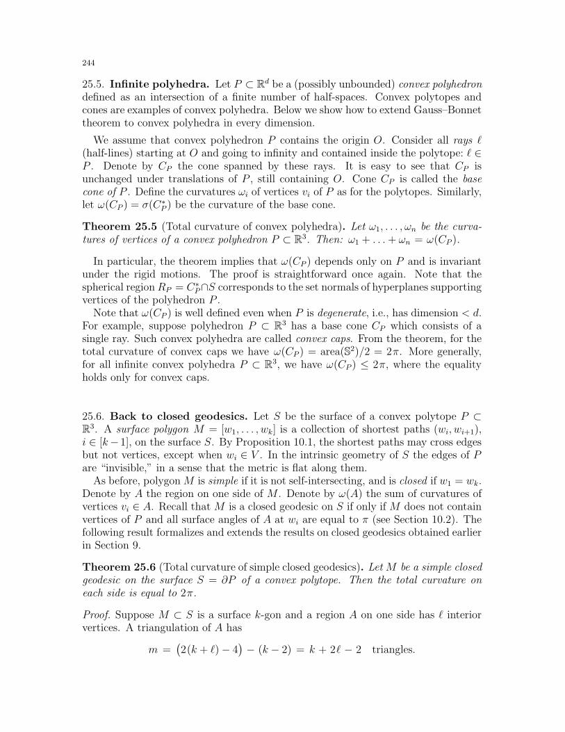
244

25.5. Infinite polyhedra. Let P ⊂ Rd be a (possibly unbounded) convex polyhedrondefined as an intersection of a finite number of half-spaces. Convex polytopes andcones are examples of convex polyhedra. Below we show how to extend Gauss–Bonnettheorem to convex polyhedra in every dimension.

We assume that convex polyhedron P contains the origin O. Consider all rays ℓ(half-lines) starting at O and going to infinity and contained inside the polytope: ℓ ∈P . Denote by CP the cone spanned by these rays. It is easy to see that CP isunchanged under translations of P , still containing O. Cone CP is called the basecone of P . Define the curvatures ωi of vertices vi of P as for the polytopes. Similarly,let ω(CP ) = σ(C∗

P ) be the curvature of the base cone.

Theorem 25.5 (Total curvature of convex polyhedra). Let ω1, . . . , ωn be the curva-tures of vertices of a convex polyhedron P ⊂ R3. Then: ω1 + . . .+ ωn = ω(CP ).

In particular, the theorem implies that ω(CP ) depends only on P and is invariantunder the rigid motions. The proof is straightforward once again. Note that thespherical regionRP = C∗

P∩S corresponds to the set normals of hyperplanes supportingvertices of the polyhedron P .

Note that ω(CP ) is well defined even when P is degenerate, i.e., has dimension < d.For example, suppose polyhedron P ⊂ R3 has a base cone CP which consists of asingle ray. Such convex polyhedra are called convex caps. From the theorem, for thetotal curvature of convex caps we have ω(CP ) = area(S2)/2 = 2π. More generally,for all infinite convex polyhedra P ⊂ R3, we have ω(CP ) ≤ 2π, where the equalityholds only for convex caps.

25.6. Back to closed geodesics. Let S be the surface of a convex polytope P ⊂R3. A surface polygon M = [w1, . . . , wk] is a collection of shortest paths (wi, wi+1),i ∈ [k−1], on the surface S. By Proposition 10.1, the shortest paths may cross edgesbut not vertices, except when wi ∈ V . In the intrinsic geometry of S the edges of Pare “invisible,” in a sense that the metric is flat along them.

As before, polygon M is simple if it is not self-intersecting, and is closed if w1 = wk.Denote by A the region on one side of M . Denote by ω(A) the sum of curvatures ofvertices vi ∈ A. Recall that M is a closed geodesic on S if only if M does not containvertices of P and all surface angles of A at wi are equal to π (see Section 10.2). Thefollowing result formalizes and extends the results on closed geodesics obtained earlierin Section 9.

Theorem 25.6 (Total curvature of simple closed geodesics). Let M be a simple closedgeodesic on the surface S = ∂P of a convex polytope. Then the total curvature oneach side is equal to 2π.

Proof. Suppose M ⊂ S is a surface k-gon and a region A on one side has ℓ interiorvertices. A triangulation of A has

m =(2(k + ℓ)− 4

)− (k − 2) = k + 2ℓ − 2 triangles.

245

Thus, the total sum α(A) of the face and boundary angles in A satisfies α(A) = mπ.On the other hand, summing over all vertices, we have α(A) = 2πℓ − ω(A) − kπ.Together these equations imply the result.

The proposition implies that if there is no way to split the total curvature of allvertices into two equal parts, then there are no simple closed geodesics (see Section 9).Here is another result in this direction.

Corollary 25.7. An infinite convex polyhedron P ⊂ R3 has a simple closed geodesicif and only if P is a convex cap.

Proof. The corollary follows immediately from Theorem 25.5 and the observationsabove: ω1 + . . . + ωn = ω(CP ) < 2π unless P is a convex cap. To prove the secondpart, suppose P is a convex cap. Consider a hyperplane H orthogonal to a ray CP ,and such that all vertices of P lie on one side of H . Then the intersection M = H∩∂Pis a closed geodesic.

The following is a somewhat unexpected application of the proposition.

Theorem 25.8 (Cohn-Vossen). Two simple closed geodesics on a surface of a convexpolytope either intersect or have equal lengths.

For example, a hexagon and a square shown in Figure 10.4 are two closed geodesicson a cube of different length, and they do, in fact, intersect. The theorem also allowsan easy calculation of the lengths of geodesics. For example, in a regular tetrahedronin the same figure, the rectangular geodesics can be sled down towards an edge. Thusits length is twice the edge length.

Proof. Let P be a convex polytope, and let M1,M2 be two simple closed geodesicson the surface S of P . As before, let V be the set of vertices of P . Assume that M1

and M2 do not intersect. Then polygons M1 and M2 divide the surface S into threeregions: B1, B2 and C, such that ∂B1 = M1, ∂B2 = M2, and ∂C = M1 ∪M2. Byproposition, the sum of curvatures inside B1 and B2 is equal to 2π, so by the Gauss–Bonnet theorem region C does not have interior points.

In the language of the graph G = (V,E) of P , observe that the sets of interiorvertices V1 = V (B1) and V2 = V (B2) are disjoint, nonempty and contain all graphvertices: V = V1 ∪ V2. Thus, there exists an edge (x, y) ∈ E, such that x ∈ V1,y ∈ V2 Since both M1 and M2 must intersect (x, y), denote by z1, z2 points of in-tersection. Now cut the region C with an interval (z1, z2), and unfold C on a plane(see Figure 25.2). Each geodesic becomes a straight interval (z1, z

′1) and (z2, z

′2),

where (z′1, z′2) used to be identified with (z1, z2). Thus, the unfolding is a plane 4-gon

Z = [z1z′1z

′2z2] with |z1z2| = |z′1z′2|. Since M1 and M2 are both geodesics, we have:

∠ z′1z1z2 + ∠ z1z′1z

′2 = ∠ z1z2z

′2 + ∠ z′1z

′2z2 = π .

Therefore, Z is a parallelogram and geodesics M1 and M2 have equal length.

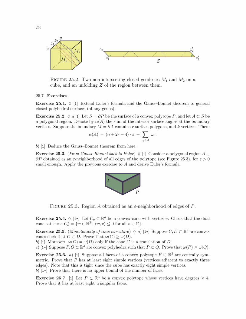
246

Z

y

x

M1

M2

z1

z1z2

z2

z′2

z′1

Figure 25.2. Two non-intersecting closed geodesics M1 and M2 on acube, and an unfolding Z of the region between them.

25.7. Exercises.

Exercise 25.1. ♦ [1] Extend Euler’s formula and the Gauss–Bonnet theorem to generalclosed polyhedral surfaces (of any genus).

Exercise 25.2. ♦ a [1] Let S = ∂P be the surface of a convex polytope P , and let A ⊂ S bea polygonal region. Denote by α(A) the sum of the interior surface angles at the boundaryvertices. Suppose the boundary M = ∂A contains r surface polygons, and k vertices. Then:

α(A) = (n+ 2r − 4) · π +∑

vi∈Aωi .

b) [1] Deduce the Gauss–Bonnet theorem from here.

Exercise 25.3. (From Gauss–Bonnet back to Euler) ♦ [1] Consider a polygonal region A ⊂∂P obtained as an ε-neighborhood of all edges of the polytope (see Figure 25.3), for ε > 0small enough. Apply the previous exercise to A and derive Euler’s formula.

P

A

Figure 25.3. Region A obtained as an ε-neighborhood of edges of P .

Exercise 25.4. ♦ [1-] Let Cv ⊂ Rd be a convex cone with vertex v. Check that the dualcone satisfies: C∗

v = w ∈ R3 | 〈w, v〉 ≤ 0 for all v ∈ C.Exercise 25.5. (Monotonicity of cone curvature) ♦ a) [1-] Suppose C,D ⊂ Rd are convexcones such that C ⊂ D. Prove that ω(C) ≥ ω(D).b) [1] Moreover, ω(C) = ω(D) only if the cone C is a translation of D.c) [1-] Suppose P,Q ⊂ Rd are convex polyhedra such that P ⊂ Q. Prove that ω(P ) ≥ ω(Q).

Exercise 25.6. a) [1] Suppose all faces of a convex polytope P ⊂ R3 are centrally sym-metric. Prove that P has at least eight simple vertices (vertices adjacent to exactly threeedges). Note that this is tight since the cube has exactly eight simple vertices.b) [1-] Prove that there is no upper bound of the number of faces.

Exercise 25.7. [1] Let P ⊂ R3 be a convex polytope whose vertices have degrees ≥ 4.Prove that it has at least eight triangular faces.

247

Exercise 25.8. Let P ⊂ R3 be a convex polytope. Denote by c(P ) the sum of the numberof triangular faces and the number of vertices of degree 3.a) [1-] Check that the graph-theoretic proof in Subsection 11.2 implies that c(P ) ≥ 1.b) [1] Use Euler’s formula to prove that c(P ) ≥ 8.

Exercise 25.9. a) [1] Suppose the surface S of a convex polytope P ⊂ R3 can be decom-posed into a finite number of rectangles. Prove that P has at most eight vertices.b) [1] Suppose S can be decomposed into a finite number of rectangles. Prove that P hasat most twelve vertices.

Exercise 25.10. (de Gua’s formula) [1] Let P ⊂ R3 be a convex polytope. Denote by Aand B the sums of all solid and dihedral angles, respectively. Prove that

2B − A = 2π(m − 2),

where m is the number of faces in P .

Exercise 25.11. Let P ⊂ R3 be a convex polytope containing the origin O. For a facet Fof P , denote by α(F ) the sum of the angles of F and by β(F ) the sum of the angles of theprojection of F onto a unit sphere centered at O. Finally, let ω(F ) = β(F ) − α(F ). Provethat ∑

F⊂Pω(F ) = 4π.

Exercise 25.12. (Equihedral tetrahedra) ♦ [1+] Let ∆ ⊂ R3 be a tetrahedron. Prove thatthe following conditions are equivalent:

(i) all faces of ∆ are congruent triangles,(ii) all faces have equal perimeter,(iii) all vertices have equal curvature,(iv) the opposite edges have equal dihedral angles,(v) all solid angles are equal.

Such ∆ are called equihedral tetrahedra.

Exercise 25.13. [1+] The edges of a convex polytope P ⊂ R3 are colored with two colors.Prove that there exists a vertex in P such that the adjacent edges either have the samecolor or have two color intervals (in cyclic order).

Exercise 25.14. [1] Let Γ be the graph of a convex polytope P ⊂ R3 and let O be anorientation of edges. As always, let V and F denote the set of vertices and faces of P . For avertex v ∈ V , denote by ind(v) to be 1− c(v)/2, where c(v) is the number of changes in theorientation of edges adjacent to v (in cyclic order). Similarly, for a face F ∈ F , denote byind(F ) to be 1− c(F )/2, where c(F ) is the number of changes in the orientation (clockwisevs. counterclockwise) of edges of F . Prove that

∑

v∈Vind(v) +

∑

F∈Find(F ) = 2.

Exercise 25.15. (Discrete Poincare–Hopf index theorem) a) [1] Let P ⊂ R3 be a convexpolytope. We say that an orientation of edges of P is balanced if every vertex has at least oneingoing and one outgoing edge (i.e., the oriented graph of P has no sinks and no sources).Prove that the edges of at least two faces of P form oriented cycles.b) [1] Generalize part a) to orientable 2-dimensional polyhedral surfaces of higher genus.

248

Exercise 25.16. [1] Prove that the inverse to Theorem 25.6 does not hold, i.e., constructa convex polytope P such that a subset of vertices has sum of curvatures equal to 2π, butwhich has no simple closed geodesics.

Exercise 25.17. [1+] Let P ⊂ R3 be an unbounded polyhedron with σ(CP ) > 0. Provethat between every two points in S = ∂P there is only a finite number of geodesics.

Exercise 25.18. Let γ denote the largest dihedral angle in a convex polytope P ⊂ R3

with n vertices.a) [1] Suppose γ < π/2. Prove that P is a tetrahedron.b) [1] Suppose γ ≤ π/2. Prove that n ≤ 8.c) [1+] Suppose γ ≤ π − ε, for some ε > 0. Disprove: n is bounded as a function of ε.

Exercise 25.19. [1+] Suppose integers n,m, k > 0 satisfy n−m+ k = 2, n ≥ 2k − 4, andk ≥ 2n− 4. Give a direct construction of a convex polytope in R3 with n vertices, m edgesand k faces.

Exercise 25.20. (Eberhard’s theorem) a) [1] Use Euler’s formula to show that for everysimple polytope P ⊂ R3, we have:

∑

i≥3

(6− i) · fi(P ) = 12,

where fi(P ) is the number of faces with k sides.b) [2] Suppose (f3, f4, . . .) is an integer sequence which satisfies the above equation. Usethe Steinitz theorem (Theorem 11.1) to prove that there exists a simple polytope P ⊂ R3,such that fi(P ) = fi for all i 6= 6.

25.8. Final remarks. Our presentation of Euler’s and Gauss–Bonnet theorems is a vari-ation on a standard theme (see [SCY, §57], [Hop2] and [Ber1, §12.7]). The curvature ωiis the discrete version of the classical Gaussian curvature, and is usually called the angledefect.

The Gauss–Bonnet theorem for 3-dimensional convex polyhedra (Theorem 25.3) is dueto Descartes [Fed], so it precedes Euler’s formula by over a century. In fact, the sphericalgeometry proof of Euler’s theorem is due to Legendre, and is probably the oldest rigorousproof (see [Bla2, Crom] for more on the history of the subject). The extension of the Gauss–Bonnet theorem to general polyhedra (Theorem 25.5) will be used at a technical point inthe proof of the main result in Section 35. See [A2, §1.5] for 3-dimensional treatment. Thehigher dimensional generalization (Theorem 25.4) is due to Shephard [Gru4].

The idea of taking an ε-neighborhood in Exercise 25.3 is standard in geometry. In asimilar context it leads to an advanced generalization of the Gauss–Bonnet theorem to alleven-dimensional Riemannian manifolds [Gray, §5.5]. We refer to [Gray, §5.6] for the historyof the Gauss–Bonnet theorem, various extensions and further references. Theorems 25.6and 25.8 are essentially due to Cohn-Vossen [CV]. Although he does not consider convexpolyhedral surfaces, his study of geodesics on Riemann surfaces have polyhedral analogues(see [Bus] for further results and references).

The formula in Exercise 25.10 is due to de Gua (1783) and can be generalized to higher

dimensions by scaling the angles and taking the alternating sum (see [Gru4]). For an

interesting discussion on the nature of Euler’s formula see also [Lak].

249

26. Cauchy theorem: the statement, the proof, and the story

In this section we give the classical proof of the Cauchy theorem, of Alexandrov’sextension, and of Stoker’s converse. Much of the rest of the book is based on thissection.

26.1. Polytopes are surprisingly rigid. Let P and P ′ be two combinatoriallyequivalent polytopes in R3 (see Section 12), with vertices v1, . . . , vn and v′1, . . . , v

′n,

and faces F1, . . . , Fm and F ′1, . . . , F

′m, respectively. From here on, we will always

assume that the equivalence maps the corresponding vertices and the correspondingfaces, i.e., vi → v′i and Fj → F ′

j , all i and j. Finally, suppose the correspondingvertices belong to the corresponding faces: vi ∈ Fj if and only if v′i ∈ F ′

j . We say thattwo faces Fj and F ′

j are equal if they are equal as polygons, i.e., the correspondingedges have equal lengths and the corresponding face angles are equal.

Theorem 26.1 (Cauchy theorem). Let P and P ′ ⊂ R3 be two convex polytopes asabove, with all faces equal polygons: Fj ≃ F ′

j, for all 1 ≤ j ≤ m. Then P and P ′ areequal polytopes: P ≃ P ′, i.e., P can be moved into P ′ by a rigid motion.

There is a way to think of the Cauchy theorem in terms of graph realizability.Suppose P is simplicial, i.e., all faces are triangles. Then faces are determined by theedge lengths. Formally, let G be the graph of P , and let L : E → R+ be the lengthfunction on edges of P . The Cauchy theorem implies that if convex polytope P ′ hasthe same pair (G,L), then P ≃ P ′. In other words, polytope P with (G,L) is uniqueup to a rigid motion. This uniqueness property is an important way of thinking ofTheorem 26.1.

More generally, let T be a graph of some triangulation of faces of P , i.e., a graph onthe set V of vertices of P with the set of edges H ⊃ E being edges of the polytope andsome diagonals in T . Denote by L : H → R+ be the corresponding length function.Now the full power of the Cauchy theorem implies that if convex polytope P ′ has thesame pair (T, L), then P ≃ P ′.

A more traditional way to think of the Cauchy theorem is in terms of (continuous)rigidity. A continuous family of polytopes Pt : t ∈ [0, 1] is called a continuousdeformation of P0 into P1 if under deformation the faces remain equal. The Cauchytheorem now implies the following result.

Corollary 26.2 (Rigidity of convex polytopes). Let Pt : t ∈ [0, 1] be a continuousdeformation of convex polytopes. Then Pt is a rigid transformation from P0 to P1.

While the corollary follows immediately from the Cauchy theorem, it is easier toprove, has many applications and generalizations, some of which will be mentionedbelow.

Remark 26.3. Let us calculate the degrees of freedom of convex polytopes to see if theCauchy theorem makes sense. A simplicial polytope P ⊂ R3 is determined by its 3ncoordinates. The space of rigid motions has dim O(3,R) = 6 dimensions (three rotationsaround pairs of axes and three translations along the axes). Thus, up to a rigid motion,polytope P has 3n − 6 degrees of freedom. Since the number of edges is |E| = 3n − 6,

250

this makes sense (see Corollary 25.2). If we had |E| < 3n − 6, we would have a hard timeshowing that they have a unique real solution.65 While this is not a formal argument, the‘magic number’ (3n − 6) is good to keep in mind.

26.2. What to expect when you are expecting a proof. Surprise! There aremany interesting proofs of the Cauchy theorem and its relatives. The classical proof(essentially due to Cauchy) will occupy the rest of this section. As the reader shallsee in the next section, the Cauchy theorem can be extended and generalized in anumber of ways. We outline a few of these directions and prove some extensions.

In fact, much of the rest of the book is also connected to the Cauchy theorem, oneway or another, but the following seven sections are directly related. In Sections 28, 29we present two other proofs of the Cauchy theorem, one of a ‘local’, while another of‘global’ nature. In Section 30 we present several examples of non-unique and flexiblepolyhedra. By the Cauchy theorem these polyhedra must be non-convex, but theyare interesting and enlightening nonetheless.

Later, in Section 31, we introduce an algebraic approach to rigidity of polyhedra.This approach leads us to two proofs of Dehn’s rigidity theorem (in Sections 32 and 33)and eventually culminates in Section 34 with the proof of the bellows conjecture(Theorem 31.2). Let us note that the final remarks subsections in these sectionscontain references not listed in other sections, so the reader is advised to read all ofthem to get the “big picture”.

26.3. The traditional proof of the Cauchy theorem. Let P and P ′ be twopolytopes as in the Cauchy theorem (Theorem 26.1). Denote by G = (V,E) thegraph of P (and of P ′), and by αe and α′

e the dihedral angles in polytopes P and P ′

of the corresponding edge e ∈ E. Let us label every edge e ∈ E with (+) if αe < α′e,

with (−) if αe > α′e, and with (0) if αe = α′

e. Now let us analyze this labeled graph G.For a vertex v in P , consider the labels of the edges containing v, written in cyclical

order, and ignoring the zero labels. Denote by mv the number of sign changes, i.e.,pairs of adjacent edges (cyclically, skipping all 0’s) with labels of different signs (seee.g., Figure 26.1). Clearly, mv is always even.

Lemma 26.4 (Sign changes lemma). For every vertex v ∈ V , the number of signchanges mv among pairs of edges containing v is at least four, unless all labels ofedges containing v are zero.

Proof. Let Cv be the cone spanned by edges of the polytope P containing v. Thinkof Cv as an infinite cone starting at v and containing P . Now let Qv be the sphericalconvex polygon obtained by intersection of Cv with a unit sphere S2 centered at v.The sides of Qv are equal to the face angles, while angles are equal to dihedral anglesin edges containing v. Note also that Qv lies in a hemisphere S2

+. Similarly, let Q′v

be the corresponding polygon obtained from P ′. From above, Qv and Q′v have equal

65The system would have infinitely many complex realizations of (G,L), but that make very littlesense in the context of convex polytopes over the real numbers.

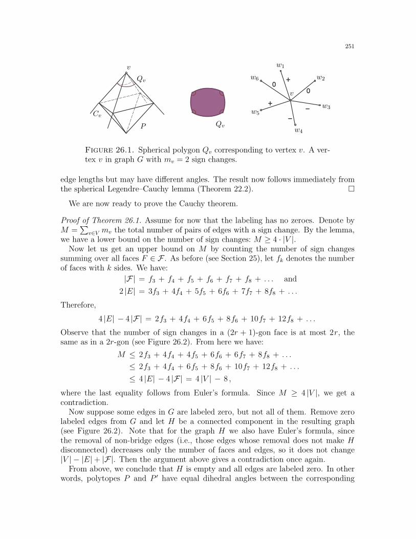
251

v

CvQv

Qv

P

+

0

-

0

+

-

w1

w2

w3

w4

w5

w6

v

Figure 26.1. Spherical polygon Qv corresponding to vertex v. A ver-tex v in graph G with mv = 2 sign changes.

edge lengths but may have different angles. The result now follows immediately fromthe spherical Legendre–Cauchy lemma (Theorem 22.2).

We are now ready to prove the Cauchy theorem.

Proof of Theorem 26.1. Assume for now that the labeling has no zeroes. Denote byM =

∑v∈V mv the total number of pairs of edges with a sign change. By the lemma,

we have a lower bound on the number of sign changes: M ≥ 4 · |V |.Now let us get an upper bound on M by counting the number of sign changes

summing over all faces F ∈ F . As before (see Section 25), let fk denotes the numberof faces with k sides. We have:

|F| = f3 + f4 + f5 + f6 + f7 + f8 + . . . and

2 |E| = 3f3 + 4f4 + 5f5 + 6f6 + 7f7 + 8f8 + . . .

Therefore,

4 |E| − 4 |F| = 2f3 + 4f4 + 6f5 + 8f6 + 10f7 + 12f8 + . . .

Observe that the number of sign changes in a (2r + 1)-gon face is at most 2r, thesame as in a 2r-gon (see Figure 26.2). From here we have:

M ≤ 2f3 + 4f4 + 4f5 + 6f6 + 6f7 + 8f8 + . . .

≤ 2f3 + 4f4 + 6f5 + 8f6 + 10f7 + 12f8 + . . .

≤ 4 |E| − 4 |F| = 4 |V | − 8 ,

where the last equality follows from Euler’s formula. Since M ≥ 4 |V |, we get acontradiction.

Now suppose some edges in G are labeled zero, but not all of them. Remove zerolabeled edges from G and let H be a connected component in the resulting graph(see Figure 26.2). Note that for the graph H we also have Euler’s formula, sincethe removal of non-bridge edges (i.e., those edges whose removal does not make Hdisconnected) decreases only the number of faces and edges, so it does not change|V | − |E|+ |F|. Then the argument above gives a contradiction once again.

From above, we conclude that H is empty and all edges are labeled zero. In otherwords, polytopes P and P ′ have equal dihedral angles between the corresponding

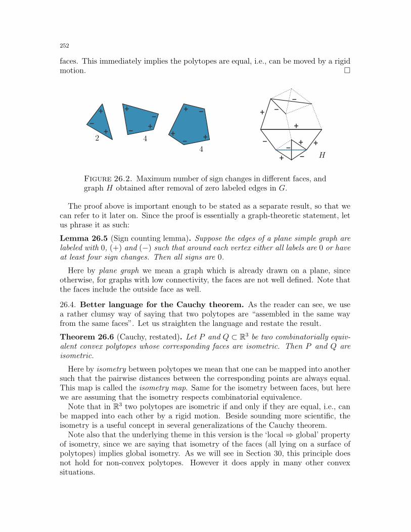
252

faces. This immediately implies the polytopes are equal, i.e., can be moved by a rigidmotion.

+

+

-

+

-+

-

+

++

-

- +-

-

+

- +-

+

-+

2 4

4H

Figure 26.2. Maximum number of sign changes in different faces, andgraph H obtained after removal of zero labeled edges in G.

The proof above is important enough to be stated as a separate result, so that wecan refer to it later on. Since the proof is essentially a graph-theoretic statement, letus phrase it as such:

Lemma 26.5 (Sign counting lemma). Suppose the edges of a plane simple graph arelabeled with 0, (+) and (−) such that around each vertex either all labels are 0 or haveat least four sign changes. Then all signs are 0.

Here by plane graph we mean a graph which is already drawn on a plane, sinceotherwise, for graphs with low connectivity, the faces are not well defined. Note thatthe faces include the outside face as well.

26.4. Better language for the Cauchy theorem. As the reader can see, we usea rather clumsy way of saying that two polytopes are “assembled in the same wayfrom the same faces”. Let us straighten the language and restate the result.

Theorem 26.6 (Cauchy, restated). Let P and Q ⊂ R3 be two combinatorially equiv-alent convex polytopes whose corresponding faces are isometric. Then P and Q areisometric.

Here by isometry between polytopes we mean that one can be mapped into anothersuch that the pairwise distances between the corresponding points are always equal.This map is called the isometry map. Same for the isometry between faces, but herewe are assuming that the isometry respects combinatorial equivalence.

Note that in R3 two polytopes are isometric if and only if they are equal, i.e., canbe mapped into each other by a rigid motion. Beside sounding more scientific, theisometry is a useful concept in several generalizations of the Cauchy theorem.

Note also that the underlying theme in this version is the ‘local⇒ global’ propertyof isometry, since we are saying that isometry of the faces (all lying on a surface ofpolytopes) implies global isometry. As we will see in Section 30, this principle doesnot hold for non-convex polytopes. However it does apply in many other convexsituations.

253

Now let us redefine rigidity of convex polytopes and restate Corollary 26.2. Wesay that Pt : t ∈ [0, 1] is a continuous deformation of polytope P if the faces of Ptremain isometric, for all t ∈ [0, 1]. We say that P is (continuously) rigid if in everycontinuous deformation Pt of polytope P the polytopes Pt are isometric.

Corollary 26.7 (Rigidity of convex polytopes, revisited). Every convex polytope P ⊂R3 is continuously rigid.

This definition of rigidity is also robust enough to allow advanced generalizations.For simplicity, we drop ‘continuous’ and use ‘rigidity’ for the rest of the lectures66.

26.5. Parallel polytopes. We start a short series of extensions of the Cauchy the-orem (Theorem 26.1) with the following side result. While easily equivalent to theCauchy theorem, it brings to light some properties of the proof given in Section 26.3.

Theorem 26.8 (Alexandrov). Let P,Q ⊂ R3 be two combinatorially equivalent con-vex polytopes with equal corresponding face angles. Then they have equal correspondingdihedral angles.

This result easily implies the Cauchy theorem: faces and dihedral angles determinethe whole polytope. In fact, we used this observation in the proof of the Cauchytheorem. On the other hand, the result is applicable to distinct polytopes, such asbricks [a× b× c].

The proof of Theorem 26.8 is essentially an observation. Note that in the proof ofthe Cauchy theorem we never used the geometry of faces, except for the face angles.In addition to the (intrinsic) convexity of polyhedra, we use only only one globalparameter: Euler’s theorem, that is a consequence from the fact that the surfaces ofconvex polytopes are homeomorphic to a sphere. Thus, basically, in the proof of theCauchy theorem, we first establish Theorem 26.8, and only then prove the result.

We say that two polytopes P,Q ∈ Rd are parallel if they are combinatorially equiv-alent and the corresponding facets are parallel. Clearly, every two combinatoriallyequivalent polytopes with equal corresponding dihedral angles can be made parallelby a rigid motion. Basically, one can view Theorem 26.8 as a local condition for beingparallel, up to a global rotation.

Let us mention that the inverse to Theorem 26.8 is also true. Given two polytopeswhich are combinatorially equivalent and have equal corresponding dihedral angleswe conclude that they are parallel, i.e., the corresponding faces lie on parallel planes.Therefore, the corresponding edges lie on parallel lines. Finally, the correspondingface angles are equal as angles between pairwise parallel lines.

26.6. Face angles are not as good as you think they are. Before we move tofurther generalizations of the Cauchy theorem, let us mention that from the point ofview of convex polytopes, face angles are not a good way to define a polytope. Infact, they overdetermine the polytope, even up to translation of faces. Indeed, let us

66There are other kinds of rigidity, such as static rigidity, infinitesimal rigidity, k-th order rigidity,global rigidity, etc. (see [Con5]). We will define the first two in Sections 31 and 33.

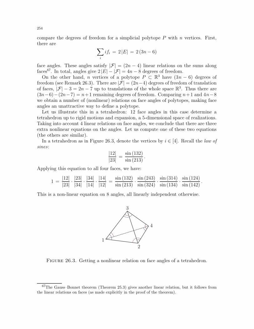
254

compare the degrees of freedom for a simplicial polytope P with n vertices. First,there are ∑

i

ifi = 2 |E| = 2(3n− 6)

face angles. These angles satisfy |F| = (2n − 4) linear relations on the sums alongfaces67. In total, angles give 2 |E| − |F| = 4n− 8 degrees of freedom.

On the other hand, n vertices of a polytope P ⊂ R3 have (3n − 6) degrees offreedom (see Remark 26.3). There are |F| = (2n−4) degrees of freedom of translationof faces, |F| − 3 = 2n − 7 up to translations of the whole space R3. Thus there are(3n−6)−(2n−7) = n+1 remaining degrees of freedom. Comparing n+1 and 4n−8we obtain a number of (nonlinear) relations on face angles of polytopes, making faceangles an unattractive way to define a polytope.

Let us illustrate this in a tetrahedron: 12 face angles in this case determine atetrahedron up to rigid motions and expansion, a 5-dimensional space of realizations.Taking into account 4 linear relations on face angles, we conclude that there are threeextra nonlinear equations on the angles. Let us compute one of these two equations(the others are similar).

In a tetrahedron as in Figure 26.3, denote the vertices by i ∈ [4]. Recall the law ofsines :

|12||23| =

sin (132)

sin (213).

Applying this equation to all four faces, we have:

1 =|12||23| ·

|23||34| ·

|34||14| ·

|14||12| =

sin (132)

sin (213)· sin (243)

sin (324)· sin (314)

sin (134)· sin (124)

sin (142).

This is a non-linear equation on 8 angles, all linearly independent otherwise.

1

2

3

4

Figure 26.3. Getting a nonlinear relation on face angles of a tetrahedron.

67The Gauss–Bonnet theorem (Theorem 25.3) gives another linear relation, but it follows fromthe linear relations on faces (as made explicitly in the proof of the theorem).

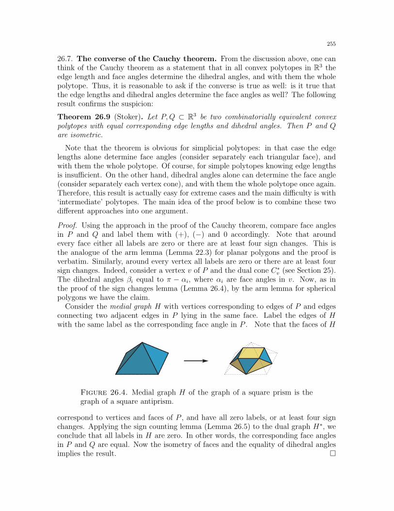
255

26.7. The converse of the Cauchy theorem. From the discussion above, one canthink of the Cauchy theorem as a statement that in all convex polytopes in R3 theedge length and face angles determine the dihedral angles, and with them the wholepolytope. Thus, it is reasonable to ask if the converse is true as well: is it true thatthe edge lengths and dihedral angles determine the face angles as well? The followingresult confirms the suspicion:

Theorem 26.9 (Stoker). Let P,Q ⊂ R3 be two combinatorially equivalent convexpolytopes with equal corresponding edge lengths and dihedral angles. Then P and Qare isometric.

Note that the theorem is obvious for simplicial polytopes: in that case the edgelengths alone determine face angles (consider separately each triangular face), andwith them the whole polytope. Of course, for simple polytopes knowing edge lengthsis insufficient. On the other hand, dihedral angles alone can determine the face angle(consider separately each vertex cone), and with them the whole polytope once again.Therefore, this result is actually easy for extreme cases and the main difficulty is with‘intermediate’ polytopes. The main idea of the proof below is to combine these twodifferent approaches into one argument.

Proof. Using the approach in the proof of the Cauchy theorem, compare face anglesin P and Q and label them with (+), (−) and 0 accordingly. Note that aroundevery face either all labels are zero or there are at least four sign changes. This isthe analogue of the arm lemma (Lemma 22.3) for planar polygons and the proof isverbatim. Similarly, around every vertex all labels are zero or there are at least foursign changes. Indeed, consider a vertex v of P and the dual cone C∗

v (see Section 25).The dihedral angles βi equal to π − αi, where αi are face angles in v. Now, as inthe proof of the sign changes lemma (Lemma 26.4), by the arm lemma for sphericalpolygons we have the claim.

Consider the medial graph H with vertices corresponding to edges of P and edgesconnecting two adjacent edges in P lying in the same face. Label the edges of Hwith the same label as the corresponding face angle in P . Note that the faces of H

Figure 26.4. Medial graph H of the graph of a square prism is thegraph of a square antiprism.

correspond to vertices and faces of P , and have all zero labels, or at least four signchanges. Applying the sign counting lemma (Lemma 26.5) to the dual graph H∗, weconclude that all labels in H are zero. In other words, the corresponding face anglesin P and Q are equal. Now the isometry of faces and the equality of dihedral anglesimplies the result.

256

26.8. Exercises.

Exercise 26.1. (Stoker’s conjecture) ♦ The conjecture states that every two combinatori-ally equivalent convex polytopes in R3 with equal corresponding dihedral angles have equalcorresponding face angles.a) [1-] Check that the conjecture implies Theorem 26.9.b) [1] Prove that the conjecture holds for simple polytopes.c) [1+] Prove that the conjecture holds for circumscribed polytopes.d) [∗] Prove the conjecture for simplicial polytopes.

Exercise 26.2. [1+] State the spherical analogue of Stoker’s conjecture. Find a counterex-ample.

26.9. Final remarks. The Cauchy theorem was proposed to Cauchy by Legendre, whoestablished it in several special cases (see [Bla2, Mi3]). Legendre wrote a standard geometrycourse, and was led to the problem by trying to formalize (and prove) Definition 11.10 fromEuclid’s “Elements” [Euc]:

Equal and similar solid figures are those contained bysimilar planes equal in multitude and in magnitude.

Here by “planes” Euclid means the faces of the polytope, which he required to be equalpolygons. For centuries this definition was viewed as a claim that polytopes with equal facesare equal. However, the notion of equality as congruence of polytopes is absent in Euclid,and the statement really concerns the volumes of polytopes. As was noted in [Mi3, §2.5],it seems Euclid meant to apply the definition only to volumes of “basic” polytopes, suchas triangular prisms and pyramids. In any event, Legendre proved the Cauchy theorem inseveral special cases, and gave the general problem to his student Cauchy.68

The proof of the Cauchy theorem more or less follows Cauchy’s original approach. TheAlexandrov theorem (Theorem 27.7) can be found in [A2]. Let us mention that similarpolytopes play an important role in the study of mixed volumes of convex bodies. We usethem in the proof of the Minkowski theorem (Theorem 36.2).

Our proof of Theorem 26.9 follows the original proof by Stoker, who further conjecturedthat convex polytopes with equal corresponding dihedral angles have equal face angles [Sto,§6] (see Exercise 26.1). Let us mention that Theorem 26.8 extends verbatim to S3 and H3

(see Subsection 27.1), and so does Stoker’s theorem (Theorem 26.9). Although the naturalanalogue of Stoker’s conjecture is open in full generality, the spherical analogue in false (seeExercise 26.2), and the infinitesimal version was recently established in [MazM] (see also[Ale6, §5], [Schl2] and Exercise 32.2).

In the next several sections we present further results on rigidity of polyhedral surfaces.

In Sections 28, 29 we present two other (more involved) proofs of the Cauchy theorem, and

in Sections 32, 33 we present about four different (and somewhat less involved) proofs of

the rigidity of convex polytopes (Corollary 26.2).

68The works of Legendre were studied by I.Kh. Sabitov (personal communication).

257

27. Cauchy theorem: extensions and generalizations

In this short section we discuss a number of extensions of the Cauchy theorem,some easy and straightforward, some important (the Alexandrov uniqueness theoremand its converse in Section 37) and some beyond the scope of this book (the Pogorelovuniqueness theorem).

27.1. Spherical polyhedra. As it turns out, in order to extend the Cauchy theoremto higher dimensions, we first need a spherical analogue.

Note first that the proof of the Cauchy theorem is robust enough to work in othergeometries, e.g., on a sphere S3, Lobachevsky space H3, as well as other metric spaceswith bounded curvature.

We begin with the definitions. Let Sd ⊂ Rd+1 be a d-dimensional unit sphere.A convex spherical d-dimensional polyhedron P ⊂ Sd is an intersection of a finitenumber of hemispheres Sd+, i.e., half-spheres lying on one side of a hyperplane in R4

containing the origin O. Note that the boundaries of these hemispheres are the(d − 1)-dimensional spheres, which we denote by C1, . . . , Cm. The vertices, edgesand k-dimensional faces of a convex spherical polytope P ⊂ Sd are the points ofthe boundary ∂P which lie in the intersections of d, d − 1, and d − k spheres Ci,respectively. We can now define combinatorially equivalent spherical polyhedra thesame way as we do in the Euclidian space.

Define the spherical distance between points x, y ∈ Sd as the length of the shortestpath between them. Equivalently, this is the length along the unique great circle whichcontains x, y (such circle is unique unless the points are equal or opposite). Definenow isometric spherical polyhedra, write P ≃ Q, the same way as before. Notethat spherical polyhedra P,Q ⊂ Sd are (globally) isometric if and only if there is anorthogonal transformation M ∈ O(d + 1,R) which maps P into Q, i.e. M(P ) = Q.We will need the isometry only for d = 2 (faces), and d = 3 (polytopes).

Theorem 27.1 (Cauchy theorem for spherical polyhedra). Let P,Q ⊂ S3+ be two

combinatorially equivalent convex spherical polyhedra in the upper hemisphere, whosecorresponding faces are isometric. Then P and Q are isometric.

The proof follows verbatim the proof of the Cauchy theorem, with appropriatesubstitutions of spherical geometry concepts, such as dihedral angles in edges of Pand Q. We skip the details.

27.2. Cauchy theorem in higher dimensions. We are now ready to present thefollowing important extension.

Theorem 27.2 (Cauchy theorem in higher dimensions). Let P,Q ⊂ Rd (or P,Q ⊂Sd+), d ≥ 3 be two combinatorially equivalent (spherical ) convex polyhedra whosecorresponding facets are isometric. Then P and Q are isometric.

Here by (global) isometry between polyhedra we mean that one can be mappedinto another such that the pairwise distances between the corresponding points arealways equal. By Sd+ we denote a fixed (upper) hemisphere.

258

Now, to prove Theorem 27.2, we need the corresponding result for convex sphericalpolytopes first. Such a result is easy to prove by a straightforward induction. Ford = 3 this is Theorem 27.1. Suppose the result is established for some d ≥ 3. Take a(d+ 1)-dimensional spherical polyhedron P and let Qv be an intersection of P and ad-dimensional sphere centered at a vertex v of small radius. By inductive assumptionapplied to the d-dimensional convex spherical polytope Qv, we conclude that Qv andthus the spherical pyramid Pv = convv,Qv ⊂ Sd+1 are completely determined. Thisgives the Cauchy theorem in any dimension for spherical polytopes.

Now, for a Euclidean polytope P ⊂ Rd, again consider an intersection Qv with asmall (d − 1)-dimensional sphere. Use the result for spherical polyhedra to concludethat the pyramid Pv over Qv is completely determined, and thus gives all dihedralangles between facets. We omit the details.

Before we conclude, let us state the rigidity of higher-dimensional polytopes as well.

Corollary 27.3 (Rigidity in Rd). Every convex polytope in Rd, d ≥ 3, is rigid.

Remark 27.4. There is a case to be made that in higher dimensions the polytopes arelargely overdetermined, i.e., conditions in the corollary can be weakened in most cases.Without making this precise, let us make a counting argument calculating the degrees offreedom (cf. Remark 26.3).

Consider a convex simplicial polytope P ∈ Rd, in which case the facets are determinedby the edge lengths. Suppose P has n vertices and k edges. The space of realizations ofthe graph of P up to rigid motions is dn−

(d+12

), since the dimension of the group of rigid

motions (translations and rotations) is d+ dim O(d,R) = d(d+ 1)/2. Now the rigidity of Pimplies69 that this is the lower bound for the number of edges:

() k ≥ dn−(d+ 1

2

).

Interestingly, we already have seen this inequality. Denote by P ∗ ⊂ Rd a dual polytope to P .Clearly, P ∗ is simple, and in the notation of Section 8 we have fd−1 = n and fd−2 = k.Thus, the inequality g2 ≥ g1 presented in Remark 8.2 becomes inequality () given above.

Let us show that inequality () can be quite weak. This means that a polytope canhave too many edges, more than necessary to justify the rigidity. The easiest example is across-polytope Cd ⊂ Rd, defined as a regular polytope dual to a cube. For example, C3 isa regular octahedron. Clearly, Cd has n = 2d vertices and k =

(2d2

)− d edges, making ()

into strict inequality for d ≥ 4.

27.3. Unbounded convex polyhedra. Recall the notion of (unbounded) convexpolyhedra considered in Section 25. Namely, let P ⊂ R3 be an intersection of a finitenumber of half-spaces. The question is: can we extend the Cauchy theorem to thiscase? Phrased differently, do there exist non-isometric convex polyhedra which arecombinatorially equivalent and have isometric corresponding faces?

The answer is easily “no”, and examples include a cone and a product of an un-bounded convex polygon and a line (see Figure 27.1). Somewhat surprisingly, thereis an easy way to enforce rigidity and generalize the Cauchy theorem to this case.

69Formally speaking, this conclusion can be made for realizations only over C, rather than over R.The reader can think of this as a heuristic argument which can in fact be formalized.

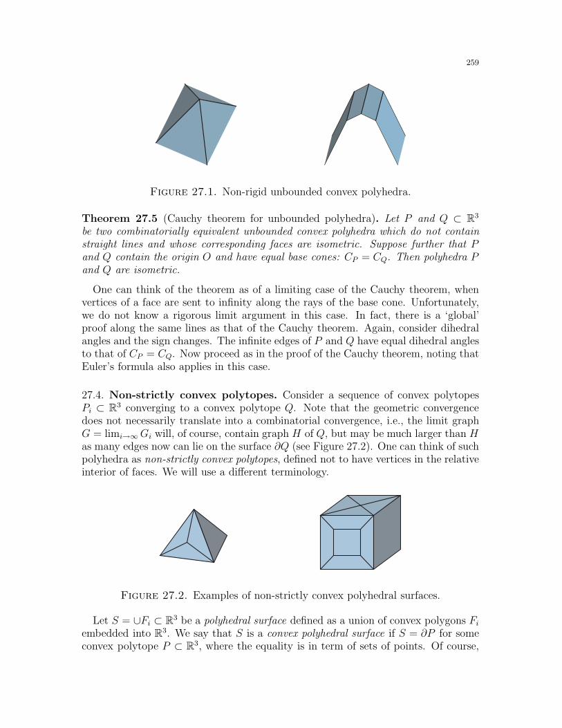
259

Figure 27.1. Non-rigid unbounded convex polyhedra.

Theorem 27.5 (Cauchy theorem for unbounded polyhedra). Let P and Q ⊂ R3

be two combinatorially equivalent unbounded convex polyhedra which do not containstraight lines and whose corresponding faces are isometric. Suppose further that Pand Q contain the origin O and have equal base cones: CP = CQ. Then polyhedra Pand Q are isometric.

One can think of the theorem as of a limiting case of the Cauchy theorem, whenvertices of a face are sent to infinity along the rays of the base cone. Unfortunately,we do not know a rigorous limit argument in this case. In fact, there is a ‘global’proof along the same lines as that of the Cauchy theorem. Again, consider dihedralangles and the sign changes. The infinite edges of P and Q have equal dihedral anglesto that of CP = CQ. Now proceed as in the proof of the Cauchy theorem, noting thatEuler’s formula also applies in this case.

27.4. Non-strictly convex polytopes. Consider a sequence of convex polytopesPi ⊂ R3 converging to a convex polytope Q. Note that the geometric convergencedoes not necessarily translate into a combinatorial convergence, i.e., the limit graphG = limi→∞Gi will, of course, contain graph H of Q, but may be much larger than Has many edges now can lie on the surface ∂Q (see Figure 27.2). One can think of suchpolyhedra as non-strictly convex polytopes, defined not to have vertices in the relativeinterior of faces. We will use a different terminology.

Figure 27.2. Examples of non-strictly convex polyhedral surfaces.

Let S = ∪Fi ⊂ R3 be a polyhedral surface defined as a union of convex polygons Fiembedded into R3. We say that S is a convex polyhedral surface if S = ∂P for someconvex polytope P ⊂ R3, where the equality is in term of sets of points. Of course,

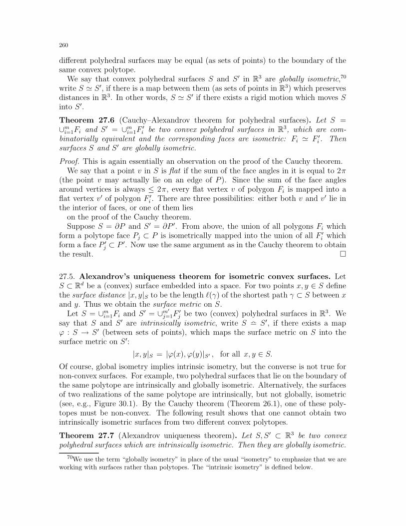
260

different polyhedral surfaces may be equal (as sets of points) to the boundary of thesame convex polytope.

We say that convex polyhedral surfaces S and S ′ in R3 are globally isometric,70

write S ≃ S ′, if there is a map between them (as sets of points in R3) which preservesdistances in R3. In other words, S ≃ S ′ if there exists a rigid motion which moves Sinto S ′.

Theorem 27.6 (Cauchy–Alexandrov theorem for polyhedral surfaces). Let S =∪mi=1Fi and S ′ = ∪mi=1F

′i be two convex polyhedral surfaces in R3, which are com-

binatorially equivalent and the corresponding faces are isometric: Fi ≃ F ′i . Then

surfaces S and S ′ are globally isometric.

Proof. This is again essentially an observation on the proof of the Cauchy theorem.We say that a point v in S is flat if the sum of the face angles in it is equal to 2π

(the point v may actually lie on an edge of P ). Since the sum of the face anglesaround vertices is always ≤ 2π, every flat vertex v of polygon Fi is mapped into aflat vertex v′ of polygon F ′

i . There are three possibilities: either both v and v′ lie inthe interior of faces, or one of them lies

on the proof of the Cauchy theorem.Suppose S = ∂P and S ′ = ∂P ′. From above, the union of all polygons Fi which

form a polytope face Pj ⊂ P is isometrically mapped into the union of all F ′i which

form a face P ′j ⊂ P ′. Now use the same argument as in the Cauchy theorem to obtain

the result.

27.5. Alexandrov’s uniqueness theorem for isometric convex surfaces. LetS ⊂ Rd be a (convex) surface embedded into a space. For two points x, y ∈ S definethe surface distance |x, y|S to be the length ℓ(γ) of the shortest path γ ⊂ S between xand y. Thus we obtain the surface metric on S.

Let S = ∪mi=1Fi and S ′ = ∪m′

j=1F′j be two (convex) polyhedral surfaces in R3. We

say that S and S ′ are intrinsically isometric, write S ≏ S ′, if there exists a mapϕ : S → S ′ (between sets of points), which maps the surface metric on S into thesurface metric on S ′:

|x, y|S = |ϕ(x), ϕ(y)|S′ , for all x, y ∈ S.Of course, global isometry implies intrinsic isometry, but the converse is not true fornon-convex surfaces. For example, two polyhedral surfaces that lie on the boundary ofthe same polytope are intrinsically and globally isometric. Alternatively, the surfacesof two realizations of the same polytope are intrinsically, but not globally, isometric(see, e.g., Figure 30.1). By the Cauchy theorem (Theorem 26.1), one of these poly-topes must be non-convex. The following result shows that one cannot obtain twointrinsically isometric surfaces from two different convex polytopes.

Theorem 27.7 (Alexandrov uniqueness theorem). Let S, S ′ ⊂ R3 be two convexpolyhedral surfaces which are intrinsically isometric. Then they are globally isometric.

70We use the term “globally isometry” in place of the usual “isometry” to emphasize that we areworking with surfaces rather than polytopes. The “intrinsic isometry” is defined below.

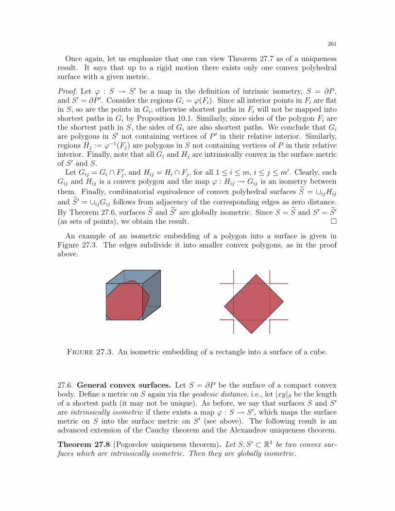
261

Once again, let us emphasize that one can view Theorem 27.7 as of a uniquenessresult. It says that up to a rigid motion there exists only one convex polyhedralsurface with a given metric.

Proof. Let ϕ : S → S ′ be a map in the definition of intrinsic isometry, S = ∂P ,and S ′ = ∂P ′. Consider the regions Gi = ϕ(Fi). Since all interior points in Fi are flatin S, so are the points in Gi; otherwise shortest paths in Fi will not be mapped intoshortest paths in Gi by Proposition 10.1. Similarly, since sides of the polygon Fi arethe shortest path in S, the sides of Gi are also shortest paths. We conclude that Gi

are polygons in S ′ not containing vertices of P ′ in their relative interior. Similarly,regions Hj := ϕ−1(Fj) are polygons in S not containing vertices of P in their relativeinterior. Finally, note that all Gi and Hj are intrinsically convex in the surface metricof S ′ and S.

Let Gij = Gi ∩ F ′j , and Hij = Hi ∩ Fj, for all 1 ≤ i ≤ m, i ≤ j ≤ m′. Clearly, each

Gij and Hij is a convex polygon and the map ϕ : Hij → Gij is an isometry between

them. Finally, combinatorial equivalence of convex polyhedral surfaces S = ∪ijHij

and S ′ = ∪ijGij follows from adjacency of the corresponding edges as zero distance.

By Theorem 27.6, surfaces S and S ′ are globally isometric. Since S = S and S ′ = S ′

(as sets of points), we obtain the result.

An example of an isometric embedding of a polygon into a surface is given inFigure 27.3. The edges subdivide it into smaller convex polygons, as in the proofabove.

Figure 27.3. An isometric embedding of a rectangle into a surface of a cube.

27.6. General convex surfaces. Let S = ∂P be the surface of a compact convexbody. Define a metric on S again via the geodesic distance, i.e., let |xy|S be the lengthof a shortest path (it may not be unique). As before, we say that surfaces S and S ′

are intrinsically isometric if there exists a map ϕ : S → S ′, which maps the surfacemetric on S into the surface metric on S ′ (see above). The following result is anadvanced extension of the Cauchy theorem and the Alexandrov uniqueness theorem.

Theorem 27.8 (Pogorelov uniqueness theorem). Let S, S ′ ⊂ R3 be two convex sur-faces which are intrinsically isometric. Then they are globally isometric.

262

The proof is a delicate and at times technical argument based on approximation ofconvex surfaces by convex polytopes. We will not present it here.

27.7. Exercises.

Exercise 27.1. [1+] Let S ⊂ R3 be a (non-convex) 2-dimensional polyhedral surface home-omorphic to a sphere, such that every face of S is a unit square. Prove that all dihedralangles of S are right angles.

Exercise 27.2. a) [1-] Prove or disprove: ∆ ⊂ R3 is a regular tetrahedron if and only ifit has five equal dihedral angles.b) [1-] The same for all six equal dihedral angles.

Exercise 27.3. (Locally convex polyhedra) ♦ [1] A polyhedron is called locally convex ifthe cone at every vertex is a convex cone. Prove that every locally convex 2-dimensionalpolyhedral surface homeomorphic to a sphere and embedded in R3 is convex.71

Exercise 27.4. [1+] Show that every two spherical tetrahedra in S3 with equal correspond-ing dihedral angles are isometric.

Exercise 27.5. ♦ [1] Complete the proof of Theorem 27.1.

Exercise 27.6. ♦ [1+] Complete the proof of Theorem 27.2.

Exercise 27.7. ♦ [1+] Complete the proof of Theorem 27.5.

Exercise 27.8. ♦ [1] Complete the proof of Theorem 27.6.

Exercise 27.9. (Olovianishnikoff ) [2] Let P ⊂ R3 be a convex polytope and let Q ⊂ R3

be a convex body. Suppose the surface ∂P is isometric to ∂Q. Prove that Q is a convexpolytope. Conclude from here that P and Q are globally isometric.

27.8. Final remarks. There are a number of extensions of the Cauchy theorem to poly-hedra in other metric spaces, some of them going back to Alexandrov, while some are morerecent and quite advanced. In particular, extensions of the Cauchy theorem to sphericalpolytopes and polytopes in a Lobachevsky space (hyperbolic polytopes) are due to Alexan-drov. We refer to [A1, A2, Pog3] for classical results, to [Con5, IKS] for the surveys, and topapers [Mi6, Mi4, Schl1] for more recent advances. Theorem 27.6 is also due to Alexandrov,as are most of the results in this section.

The study of unbounded polyhedra and Theorem 27.5 are due to Olovianishnikoff [Olo1](sometimes spelled Olovjanisnikov). He also established an important intermediate resultbetween the Alexandrov and Pogorelov uniqueness theorems in [Olo2] (see Exercise 27.9).For Pogorelov’s theorem see [Pog3].

Also, a number of further extensions of the uniqueness theorems (to convex spherical

surfaces, unbounded convex surfaces, surfaces with bounded curvature, etc.) were obtained

by Alexandrov and his students. We refer to an extensive survey [Sab1] (see also [Sen2])

for rigidity of general surfaces.

71This is unfortunate since, of course, the Cauchy rigidity theorem immediately extends to locallyconvex polyhedra homeomorphic to a sphere.

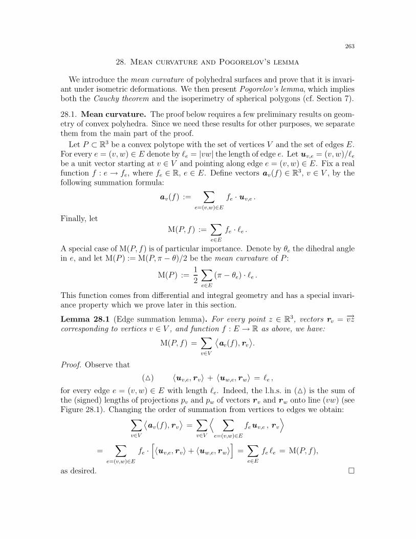
263

28. Mean curvature and Pogorelov’s lemma

We introduce the mean curvature of polyhedral surfaces and prove that it is invari-ant under isometric deformations. We then present Pogorelov’s lemma, which impliesboth the Cauchy theorem and the isoperimetry of spherical polygons (cf. Section 7).

28.1. Mean curvature. The proof below requires a few preliminary results on geom-etry of convex polyhedra. Since we need these results for other purposes, we separatethem from the main part of the proof.

Let P ⊂ R3 be a convex polytope with the set of vertices V and the set of edges E.For every e = (v, w) ∈ E denote by ℓe = |vw| the length of edge e. Let uv,e = (v, w)/ℓebe a unit vector starting at v ∈ V and pointing along edge e = (v, w) ∈ E. Fix a realfunction f : e → fe, where fe ∈ R, e ∈ E. Define vectors av(f) ∈ R3, v ∈ V , by thefollowing summation formula:

av(f) :=∑

e=(v,w)∈Efe · uv,e .

Finally, let

M(P, f) :=∑

e∈Efe · ℓe .

A special case of M(P, f) is of particular importance. Denote by θe the dihedral anglein e, and let M(P ) := M(P, π − θ)/2 be the mean curvature of P :

M(P ) :=1

2

∑

e∈E(π − θe) · ℓe .

This function comes from differential and integral geometry and has a special invari-ance property which we prove later in this section.

Lemma 28.1 (Edge summation lemma). For every point z ∈ R3, vectors rv = −→vzcorresponding to vertices v ∈ V , and function f : E → R as above, we have:

M(P, f) =∑

v∈V

⟨av(f), rv

⟩.

Proof. Observe that

() 〈uv,e, r v〉 + 〈uw,e, rw〉 = ℓe ,

for every edge e = (v, w) ∈ E with length ℓe. Indeed, the l.h.s. in () is the sum ofthe (signed) lengths of projections pv and pw of vectors r v and rw onto line (vw) (seeFigure 28.1). Changing the order of summation from vertices to edges we obtain:

∑

v∈V

⟨av(f), rv

⟩=∑

v∈V

⟨ ∑

e=(v,w)∈Efeuv,e , r v

⟩

=∑

e=(v,w)∈Efe ·[〈uv,e, r v〉+ 〈uw,e, rw〉

]=∑

e∈Efe ℓe = M(P, f),

as desired.

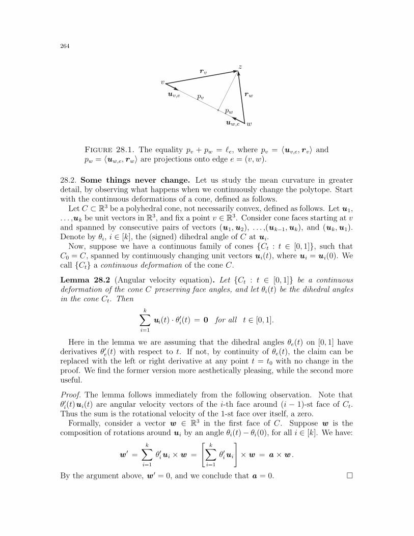
264

z

v

w

uv,e

uw,e

pv

pw

r v

rw

Figure 28.1. The equality pv + pw = ℓe, where pv = 〈uv,e, r v〉 andpw = 〈uw,e, rw〉 are projections onto edge e = (v, w).

28.2. Some things never change. Let us study the mean curvature in greaterdetail, by observing what happens when we continuously change the polytope. Startwith the continuous deformations of a cone, defined as follows.

Let C ⊂ R3 be a polyhedral cone, not necessarily convex, defined as follows. Let u1,. . . ,u k be unit vectors in R3, and fix a point v ∈ R3. Consider cone faces starting at vand spanned by consecutive pairs of vectors (u1,u2), . . . ,(u k−1,uk), and (uk,u1).Denote by θi, i ∈ [k], the (signed) dihedral angle of C at u i.

Now, suppose we have a continuous family of cones Ct : t ∈ [0, 1], such thatC0 = C, spanned by continuously changing unit vectors u i(t), where u i = u i(0). Wecall Ct a continuous deformation of the cone C.

Lemma 28.2 (Angular velocity equation). Let Ct : t ∈ [0, 1] be a continuousdeformation of the cone C preserving face angles, and let θi(t) be the dihedral anglesin the cone Ct. Then

k∑

i=1

ui(t) · θ′i(t) = 0 for all t ∈ [0, 1].

Here in the lemma we are assuming that the dihedral angles θe(t) on [0, 1] havederivatives θ′e(t) with respect to t. If not, by continuity of θe(t), the claim can bereplaced with the left or right derivative at any point t = t0 with no change in theproof. We find the former version more aesthetically pleasing, while the second moreuseful.

Proof. The lemma follows immediately from the following observation. Note thatθ′i(t)u i(t) are angular velocity vectors of the i-th face around (i − 1)-st face of Ct.Thus the sum is the rotational velocity of the 1-st face over itself, a zero.

Formally, consider a vector w ∈ R3 in the first face of C. Suppose w is thecomposition of rotations around u i by an angle θi(t)− θi(0), for all i ∈ [k]. We have:

w′ =

k∑

i=1

θ′iu i ×w =

[k∑

i=1

θ′iu i

]×w = a ×w .

By the argument above, w′ = 0, and we conclude that a = 0.

265

Before we turn to the proof of the Cauchy theorem, let us make an interestingcorollary from the lemma. Let Pt : t ∈ [0, 1] be a continuous family of combi-natorial equivalent polyhedra in R3, not necessarily convex or even embedded (seeSection 26.2), such that vertex coordinates change continuously. Then, with the samedisclaimer as after Lemma 28.2, we obtain the following result.

Theorem 28.3 (Schlafli formula). For a continuous family of polyhedra Pt : t ∈[0, 1] preserving the faces, we have:

∑

e∈Eℓe(t) · θ′e(t) = 0, for all t ∈ [0, 1],

where ℓe(t) are edge lengths and θe(t) are dihedral angles.

Proof. In the notation above, let fe = θ′e(t) be derivatives of the dihedral angles.By Lemma 28.2 we have a e(θ

′(t)) = 0, for every edge e ∈ E. On the other hand,M(Pt, θ

′(t)) =∑

e∈E ℓe(t)θ′e(t), as in the theorem. Now the edge summation lemma

(Lemma 28.1) gives:

M(Pt, θ′(t)) =

∑

v∈V

⟨av(θ

′(t)), r v⟩

= 0,

as desired.

The following corollary follows easily from the Schlafli formula, but is importantenough to single out. Recall that a continuous deformation Pt : t ∈ [0, 1] is acontinuous family of polyhedra with all edge lengths constant under deformation:ℓe(t) = ce for some ce > 0 and all t ∈ [0, 1].

Corollary 28.4 (Invariance of the mean curvature). Let Pt : t ∈ [0, 1] be a con-tinuous isometric deformation of a (possibly non-convex) polyhedron. Then the meancurvature M(Pt) is a constant independent of t.

For convex polyhedra this follows immediately from Corollary 26.7. On the otherhand, for non-convex polyhedra this is a new result, a special property of flexiblepolyhedra. We present their examples and further properties in Sections 30, 31.

Proof. Suppose first that all dihedral angles θe(t) are differentiable on [0, 1]. Then

M′(Pt) =

[1

2

∑

e∈E(π − θe) · ℓe

]′= − 1

2

∑

e∈Eℓe(t) · θ′e(t) = 0,

so the mean curvature M(Pt) is a constant independent of t. Suppose now that notall θe(t) are differentiable. By continuity, at every point t0 ∈ (0, 1) we can computethe left and right derivatives of θe(t), and then of M(Pt). From above, the left andright derivatives of M(Pt) are equal to 0 at all t ∈ (0, 1). Thus, M(Pt) is differentiablewith zero derivative in (0, 1). This again implies that M(Pt) is independent of t.

266

28.3. The ultimate local proof. Observe that the structure of the proof of theCauchy theorem splits naturally into a local and a global part: the sign changeslemma (Lemma 26.4) which easily reduces to the arm lemma (Lemma 22.3) and thesign counting lemma (Lemma 26.5) based on the use of a counting argument andEuler’s formula. There are several other proofs of the Cauchy theorem which followthe same pattern, but have varying levels of complexity of local and global parts. Theidea of this proof is to make the ‘local claim’ strong enough, so that the contradictionfollows easily, by a geometric and a straightforward double counting argument, ratherthan by a calculation and Euler’s formula. After all, Euler’s formula can also bededuced by a ‘global argument’ (see Section 25), so it makes sense that the Cauchytheorem can be proved along these lines.

Let C,D ⊂ R3 be two convex cones starting at the origin O and with the samesequence of side angles (in cyclic order). In this case we say that cones C and D haveisometric sides. The cones are called equal, write C ≃ D if there exists a rotationmapping one into the other. Finally, define the dual cone C∗ as in Subsection 25.4,to be the cone of all normal vectors: C∗ = w ∈ R3 | (w, v) ≤ 0 for all v ∈ C.

Lemma 28.5 (Pogorelov). Let C,D ⊂ R3 be two convex cones with isometric sidesand dihedral angles θ1, . . . , θk and ϑ1, . . . , ϑk, respectively. Denote by u1, . . . ,uk theunit vectors along edges of C. Let w = w(C,D) be a vector defined as follows:

w :=k∑

i=1

(ϑi − θi)ui .

Then w ∈ C∗. Furthermore, w = 0 if and only if C ≃ D.

We postpone the proof of Pogorelov’s lemma and start with the following originalproof of the Cauchy theorem based on the lemma.

Proof of the Cauchy theorem modulo Pogorelov’s lemma. Let P and Q be combina-torially equivalent convex polytopes with isometric faces. Denote by V , E the setof vertices and edges of P , respectively, and let θe denote the dihedral angles in P .To simplify the notation we use the same notation E for the sets of edges in Q andlet ϑe, e ∈ E, be the dihedral angles in Q.

Denote by Cv the cone spanned by the edges of P containing the vertex v ∈ V .Let w v be the vector as in the lemma, corresponding to the cone Cv. Fix a point z ∈ Pand let r v = (v, z), v ∈ V , be as above. Since r v ∈ Cv for all v ∈ V , by Pogorelov’slemma we have (w v, r v) ≤ 0. Summing this over all vertices, we get:

A :=∑

v∈V〈w v, r v〉 ≤ 0 .

In the notation of the edge summation lemma (Lemma 28.1), let fe = (ϑe − θe) andnote that w v = av(f). By the lemma, we have:

A =∑

e∈E(ϑe − θe) ℓe =

∑

e∈E(π − θe) ℓe −

∑

e∈E(π − ϑe) ℓe = 2M(P ) − 2M(Q),

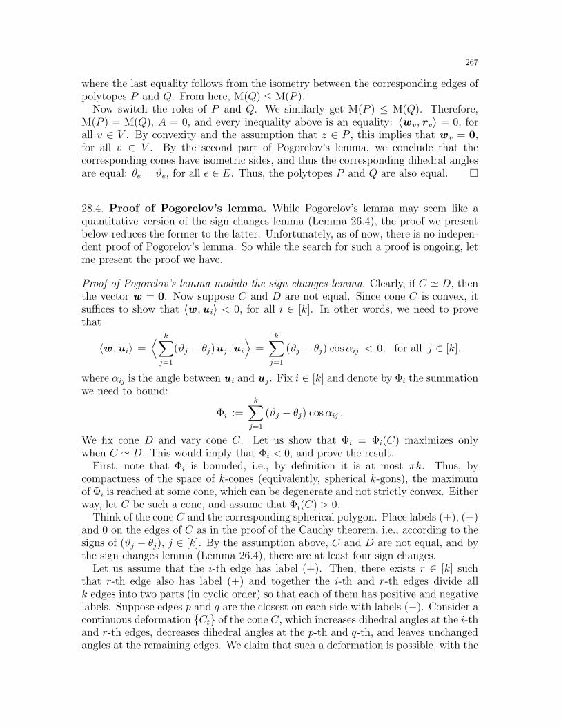
267

where the last equality follows from the isometry between the corresponding edges ofpolytopes P and Q. From here, M(Q) ≤ M(P ).

Now switch the roles of P and Q. We similarly get M(P ) ≤ M(Q). Therefore,M(P ) = M(Q), A = 0, and every inequality above is an equality: 〈w v, rv〉 = 0, forall v ∈ V . By convexity and the assumption that z ∈ P , this implies that w v = 0,for all v ∈ V . By the second part of Pogorelov’s lemma, we conclude that thecorresponding cones have isometric sides, and thus the corresponding dihedral anglesare equal: θe = ϑe, for all e ∈ E. Thus, the polytopes P and Q are also equal.

28.4. Proof of Pogorelov’s lemma. While Pogorelov’s lemma may seem like aquantitative version of the sign changes lemma (Lemma 26.4), the proof we presentbelow reduces the former to the latter. Unfortunately, as of now, there is no indepen-dent proof of Pogorelov’s lemma. So while the search for such a proof is ongoing, letme present the proof we have.

Proof of Pogorelov’s lemma modulo the sign changes lemma. Clearly, if C ≃ D, thenthe vector w = 0. Now suppose C and D are not equal. Since cone C is convex, itsuffices to show that 〈w ,u i〉 < 0, for all i ∈ [k]. In other words, we need to provethat

〈w ,u i〉 =⟨ k∑

j=1

(ϑj − θj)u j ,u i

⟩=

k∑

j=1

(ϑj − θj) cosαij < 0, for all j ∈ [k],

where αij is the angle between u i and u j. Fix i ∈ [k] and denote by Φi the summationwe need to bound:

Φi :=k∑

j=1

(ϑj − θj) cosαij .

We fix cone D and vary cone C. Let us show that Φi = Φi(C) maximizes onlywhen C ≃ D. This would imply that Φi < 0, and prove the result.

First, note that Φi is bounded, i.e., by definition it is at most πk. Thus, bycompactness of the space of k-cones (equivalently, spherical k-gons), the maximumof Φi is reached at some cone, which can be degenerate and not strictly convex. Eitherway, let C be such a cone, and assume that Φi(C) > 0.

Think of the cone C and the corresponding spherical polygon. Place labels (+), (−)and 0 on the edges of C as in the proof of the Cauchy theorem, i.e., according to thesigns of (ϑj − θj), j ∈ [k]. By the assumption above, C and D are not equal, and bythe sign changes lemma (Lemma 26.4), there are at least four sign changes.

Let us assume that the i-th edge has label (+). Then, there exists r ∈ [k] suchthat r-th edge also has label (+) and together the i-th and r-th edges divide allk edges into two parts (in cyclic order) so that each of them has positive and negativelabels. Suppose edges p and q are the closest on each side with labels (−). Consider acontinuous deformation Ct of the cone C, which increases dihedral angles at the i-thand r-th edges, decreases dihedral angles at the p-th and q-th, and leaves unchangedangles at the remaining edges. We claim that such a deformation is possible, with the

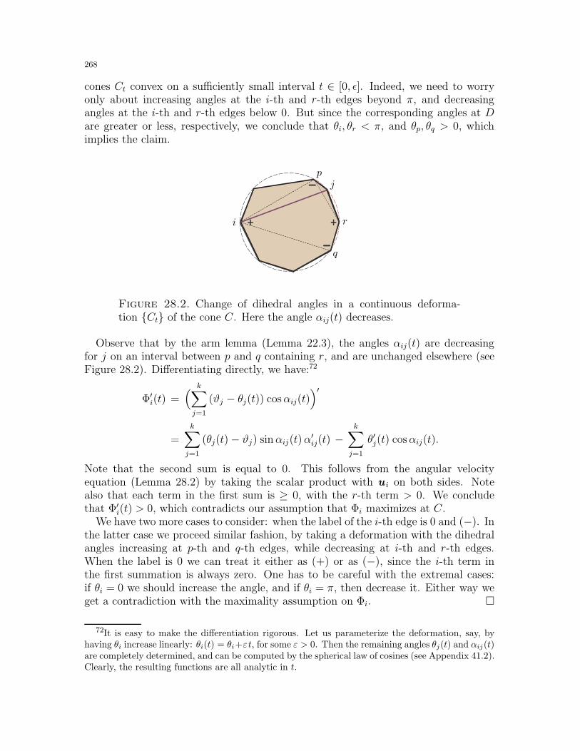
268

cones Ct convex on a sufficiently small interval t ∈ [0, ǫ]. Indeed, we need to worryonly about increasing angles at the i-th and r-th edges beyond π, and decreasingangles at the i-th and r-th edges below 0. But since the corresponding angles at Dare greater or less, respectively, we conclude that θi, θr < π, and θp, θq > 0, whichimplies the claim.

+

-

-

+i

j

r

p

q

Figure 28.2. Change of dihedral angles in a continuous deforma-tion Ct of the cone C. Here the angle αij(t) decreases.

Observe that by the arm lemma (Lemma 22.3), the angles αij(t) are decreasingfor j on an interval between p and q containing r, and are unchanged elsewhere (seeFigure 28.2). Differentiating directly, we have:72

Φ′i(t) =

( k∑

j=1

(ϑj − θj(t)) cosαij(t))′

=

k∑

j=1

(θj(t)− ϑj) sinαij(t)α′ij(t) −

k∑

j=1

θ′j(t) cosαij(t).

Note that the second sum is equal to 0. This follows from the angular velocityequation (Lemma 28.2) by taking the scalar product with u i on both sides. Notealso that each term in the first sum is ≥ 0, with the r-th term > 0. We concludethat Φ′

i(t) > 0, which contradicts our assumption that Φi maximizes at C.We have two more cases to consider: when the label of the i-th edge is 0 and (−). In

the latter case we proceed similar fashion, by taking a deformation with the dihedralangles increasing at p-th and q-th edges, while decreasing at i-th and r-th edges.When the label is 0 we can treat it either as (+) or as (−), since the i-th term inthe first summation is always zero. One has to be careful with the extremal cases:if θi = 0 we should increase the angle, and if θi = π, then decrease it. Either way weget a contradiction with the maximality assumption on Φi.

72It is easy to make the differentiation rigorous. Let us parameterize the deformation, say, byhaving θi increase linearly: θi(t) = θi+εt, for some ε > 0. Then the remaining angles θj(t) and αij(t)are completely determined, and can be computed by the spherical law of cosines (see Appendix 41.2).Clearly, the resulting functions are all analytic in t.

269

28.5. Isoperimetry of spherical polygons. The following result is classical andhas no place in this section, and fits well other isoperimetric problems in Section 7, ex-cept that the proof is a straightforward application of Pogorelov’s lemma (Lemma 28.5).

We say that two spherical polygons P,Q ⊂ S2+ are isometric if they have equal

corresponding side lengths. By restricting them to the upper hemisphere S2+ we can

define the area of the polygons as the area of the corresponding polygonal regions ona sphere.

Theorem 28.6. Let P,Q ⊂ S2+ be two isometric convex spherical polygons, such

that P is inscribed into a circle in S2 and contains its center. Then area(P ) ≥area(Q).

Proof. Denote by αi and βi the corresponding angles of polygons P and Q, i ∈ [k].By Girard’s formula (see Section 41.3) we have:

area(P ) =k∑

i=1

αi − (k − 2)π , area(Q) =k∑

i=1

βi − (k − 2)π .

Denote by O1 the center of the sphere containing convex polygons P and Q. Denoteby C and D the cones over P and Q, respectively, with center at O1. By the as-sumption, the polygon P = [x1 . . . xk] is inscribed into a circle with center O2 ∈ S2.

Finally, let r =−−−→O1O2 and u i =

−−→O1xi, for all i ∈ [k]. We have:

〈u1, r〉 = . . . = 〈uk, r〉 = c, for some c > 0.

Now, let w = w (C,D) be as in Pogorelov’s lemma:

w =k∑

i=1

(βi − αi)u i .

By the lemma, w ∈ C∗. By the assumption in the theorem, r ∈ C, and, therefore,〈w , r〉 ≤ 0. We conclude:

area(Q) − area(P ) =

k∑

i=1

(βi − αi) =

k∑

i=1

(βi − αi) ·〈u i, r〉c

=1

c

⟨ k∑

i=1

(βi − αi)u i, r⟩

=1

c〈w , r〉 ≤ 0,

as desired.

28.6. Exercises.

Exercise 28.1. ♦ [1-] Prove the result of Theorem 28.6 without the convexity assumptionon Q, and the assumption that P contains the center O2 of the circle it is inscribed into.Deduce from here the isoperimetric inequality in the plane (Theorem 7.1).

Exercise 28.2. (Monotonicity of the mean curvature) ♦ a) [1+] Let P ⊂ R3 be a convexpolytope inside a unit ball B. Denote by ℓe the length of edge e, and let γe be the dihedralangle at e. Prove that the mean curvature of P satisfies: M(P ) ≤ 4π .b) [2-] Let P,Q ⊂ R3 be two convex polytopes and P ⊂ Q. Then M(P ) ≤M(Q).

270

c) [1] Define M(X) = supP⊂XM(P ) to be the mean curvature of a convex body X. Provethat M(B) = 4π.

Exercise 28.3. a) [1+] Let C ⊂ R3 be a convex cone with a vertex at the origin. Denoteby u1, ...,uk the unit vectors along the cone edges, and let θ1, ..., θk be the correspondingdihedral angles. Prove the following inequality:

1

2

∥∥θ1u1 + . . . + θkuk∥∥ ≤ ω(C),

where ω(C) is the curvature of C.b) [1-] Use the edge summation lemma (Lemma 28.1) and the Gauss–Bonnet theorem(Theorem 25.3) to obtain part a) of Exercise 28.2.c) [∗] Generalize a) to higher dimensions.

Exercise 28.4. Let S1, S2 ⊂ R3 be two 2-dimensional polyhedral surfaces. Define theFrechet distance distF (S1, S2) as in Exercise 24.18.a) [2-] When S1, S2 are convex, prove that

∣∣M(S1) − M(S2)∣∣ ≤ 4π distF (C1, C2).

Check that this implies part a) of Exercise 28.2.b) [2] Suppose S1 and S2 are homeomorphic to a sphere. The total absolute curvature κ(S)is the sum of absolute values of curvatures of vertices in S (see Exercise 24.5). Prove that:

∣∣M(S1) − M(S2)∣∣ ≤

(κ(S1) + κ(S2) + 4π

)distF (C1, C2).

Exercise 28.5. (Minkowski formula) There is a classical differential geometry approachto the mean curvature of surfaces in Rd, but that would lead us away from the subject.Instead, we present the classical Minkowski formula which can be viewed as an alternativedefinition:

Md(P ) =

∫

Sd−1

H(u)dσ(u),

where P ⊂ Rd is a convex polytope containing the origin O, and H(u) is the supportfunction defined by H(u) = max〈x, u〉 | x ∈ P.a) [1] Prove that M2(P ) = perimeter(P ).

Now, let us compute M3(P ) by rewriting the integral as a sum over vertices. In the notationabove, using Rv = C∗

v ∩ S2, we have:

M3(P ) =∑

v∈V

∫

Rv

−〈u, r v〉dσ(u) = −∑

v∈V

⟨∫

Rv

udσ(u), r v

⟩.

b) [1+] For a simple cone C ⊂ R3 calculate the integral∫R udσ(u), where R = C ∩ S2.

c) [1+] Use additivity to compute the integral above for general cones. Write the answerfor each vertex: ∫

Rv

udσ(u) = −∑

e=(v,w)∈Eθeuv,e .

d) [1] In the edge summation lemma, let fe = θe and compute M3(P ) explicitly.

271

Exercise 28.6. (General Schlafli formula) a) [1+] Prove the Schlafli formula for every(not necessarily isometric) deformation Tt, t ∈ [0, 1] of a tetrahedron T0 ⊂ R3, i.e.,

∑

e∈Eℓe(t) · θ′e(t) = 0, for all t ∈ [0, 1].

b) [1] Deduce from here the Schlafli formula for deformations of all polyhedral surfaces.

Exercise 28.7. (Spherical Schlafli formula) a) [2-] Let T ⊂ S3 be a spherical tetrahe-dron with edge lengths ℓe and dihedral angles θe, as above. Suppose Tt, t ∈ [0, 1] is adeformation of T . Prove:

1

2

∑

e∈Eℓe(t) · θ′e(t) = vol(Tt)

′ .

b) [1] Extend this to deformations of general spherical polyhedral surfaces in S3.

Exercise 28.8. [1+] Let ∆ ⊂ R3 be a fixed tetrahedron and let a, b ⊂ ∆ denote its twoedges. When we change the length ℓa of a while keeping other edge lengths fixed, thedihedral angle θb at b also changes. Let Lab = ∂θb/∂ℓa. Prove that Lab = Lba , for all aand b.

Exercise 28.9. a) [1] Let x1, x2, x3, x4 ∈ R2 be four points in general position, and letℓij = |xixj | be the pairwise distances between them. Suppose all distances except for ℓ12and ℓ34 are fixed. Since (x1x2x3x4) has five degrees of freedom, change of ℓ12 inflicts achange of ℓ34. Prove that

ℓ12 dℓ12area(x1x2x3) · area(x1x2x4)

=− ℓ34 dℓ34

area(x1x3x4) · area(x2x3x4).

b) [1+] Let x1, x2, x3, x4, x5 ∈ R3 denote five points in general position, and let ℓij = |xixj|be as above. Suppose all ℓij except for ℓ12 and ℓ34 are fixed. Prove that

ℓ12 dℓ12vol(x1x2x3x5) · vol(x1x2x4x5)

=ℓ34 dℓ34

vol(x1x3x4x5) · vol(x2x3x4x5).

28.7. Final remarks. The angular velocity equation (Lemma 28.2) is standard, see e.g.,[A2, §10.1]. The edge summation lemma (Lemma 28.1) is a straightforward extension ofthe argument in [Pog2]. Corollary 28.4 is due to Alexander [Ale] who presented two proofs.The first proof is based on simplicial subdivisions of polyhedra and the additivity propertyof the mean curvature. Our proof of the (special case of) Schlafli formula (Theorem 28.3)is in fact similar to the second proof of Alexander (see [Ale, §9]).

The ‘local proof’ presented above is due to Pogorelov [Pog2], who never seems to havepublished the proof of his lemma (Lemma 28.5). Pogorelov’s lemma was proved in a com-panion paper [Vol1] by Volkov, which we follow. The combined Pogorelov–Volkov proofof the Cauchy theorem is obviously harder than Cauchy’s proof, since it basically replacesthe straightforward sign counting lemma (Lemma 26.5) with two non-trivial proofs (makeit four, if one counts two supporting lemmas). On the other hand, this approach has theadvantage of being connected to other results, and also gives ground for further investiga-tions.

Most recently, Schlenker found an infinitesimal analogue of Pogorelov’s lemma, and asimilar in spirit (double counting) proof of the infinitesimal rigidity [Schl4] (see Section 32).His proof of the infinitesimal analogue of Pogorelov’s lemma is independent of the signchanges lemma, and is based on some explicit calculation for spherical 4-gons. It would

272

be natural to look for a similar argument to obtain a new proof of Pogorelov’s lemma,independent of the sign changes lemma.

As we mentioned above, the fact that the mean curvature of polyhedral surfaces areinvariant under the flexing was shown in [Ale]. This result was rediscovered and extendedin [AlmR], where further connections to the Schlafli formula were found (see also [SchlS]).For the history of the Schlafli formula, references and related results see [AVS, Mil2]. Werefer to [Sant, Ch. 13] for more on mean curvature in higher dimensions, its connections todifferential and integral geometry, and the proof of the Minkowski formula (Exercise 28.5).

Our proof of Theorem 28.6 follows [Mi2] (see also [Mi3, §1.5]). Note that isoperimetric

inequalities were studied earlier in Section 7 and in fact one can view Theorem 28.6 as a

generalization of the isoperimetric inequality in the plane (see Exercise 28.1).

273

29. Sen’kin-Zalgaller’s proof of the Cauchy theorem

29.1. Avoiding counting at all cost. Below we present yet another proof of theCauchy theorem (Theorem 26.1) with the opposite philosophy compared to the proofin the previous section. Previously, of the Cauchy theorem, we replaced a simpledouble counting ‘global argument’ with a delicate and well crafted ‘local argument’(Pogorelov’s Lemma 28.5). Now, instead, we give an elaborate geometric ‘globalargument’, reducing the problem to a simple looking ‘local’ lemma, which is a weakversion of the arm lemma (Lemma 22.3). The latter will be transformed in such a wayas to allow an advanced but straightforward ‘global’ proof. This makes the followingproof fundamentally global, at least as much as such proofs ever are. We begin bystating the local result.

Lemma 29.1 (Weak arm lemma). Let X = [x1x2 . . . xn] and X ′ = [x′1x′2 . . . x

′n] be

two convex spherical polygons in the upper hemisphere, such that

∢x1x2x3 < ∢x′1x′2x

′3 , . . . , ∢xn−1xnx1 < ∢x′n−1x

′nx

′1 , ∢xnx1x2 < ∢x′nx

′1x

′2 .

Then X and X ′ are not isometric, i.e., the following equations cannot hold:

|x1x2| = |x′1x′2|, . . . , |xn−1xn| = |x′n−1x′n| , |xnx1| = |x′nx′1| .

In the notation of Section 26, the lemma says that the number of sign changescannot be zero unless all labels are zero. This case appears at the very end of theproof of the sign changes lemma (Lemma 26.4), and is an immediate consequenceof the arm lemma (Lemma 22.3). Following the pattern of the previous proofs, wecontinue with the proof of the Cauchy theorem, and then derive the lemma.

29.2. Step back and take a look from the outside. The idea of this proof isto use the global convexity of convex polytopes by comparing the distances from thesame vertex to the corresponding points on the surfaces. There are certain restrictionson this distance function which can be utilized by the following geometric argument.

Proof of the Cauchy theorem modulo the weak arm lemma. Fix any vertex v of thepolytope P , and the corresponding vertex v′ of P ′. Denote by S = ∂P and S ′ = ∂P ′

the polyhedral surfaces of the polytopes, and let ζ : S → S ′ be the isometry map asin the Cauchy theorem (Theorem 26.6). We will use primes in the notation ζ : x→ x′

between points of the surfaces throughout the proof.Consider the dual cone C∗

v (see Section 25) and fix a point w ∈ C∗v (see Figure 29.1).

Denote by f = fv : S → R+ and f ′ = f ′w : S ′ → R+ the distance function (in R3)

between v, w and points of the surfaces: f(x) = |vx|, and f ′(x′) = |wx′|. Consider asubset G = Gw ⊂ S of points where function f is greater than f ′ (on the correspondingpoints):

G := x ∈ S | f(x) > f ′(x′), wherex′ = ζ(x) .Similarly, let F = Fw ⊂ S be the set of points where the functions are equal:

F := x ∈ S | f(x) = f ′(x′), wherex′ = ζ(x) .

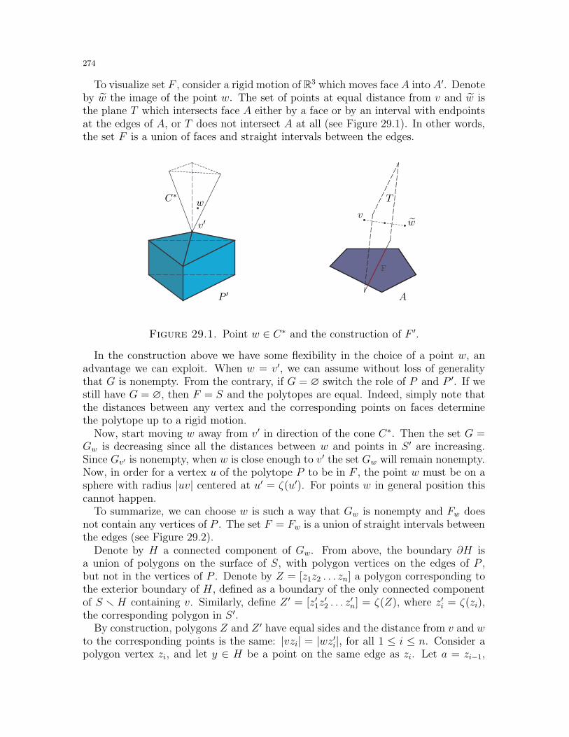
274

To visualize set F , consider a rigid motion of R3 which moves face A into A′. Denoteby w the image of the point w. The set of points at equal distance from v and w isthe plane T which intersects face A either by a face or by an interval with endpointsat the edges of A, or T does not intersect A at all (see Figure 29.1). In other words,the set F is a union of faces and straight intervals between the edges.

F

v′v

w

w

AP ′

C∗ T

Figure 29.1. Point w ∈ C∗ and the construction of F ′.

In the construction above we have some flexibility in the choice of a point w, anadvantage we can exploit. When w = v′, we can assume without loss of generalitythat G is nonempty. From the contrary, if G = ∅ switch the role of P and P ′. If westill have G = ∅, then F = S and the polytopes are equal. Indeed, simply note thatthe distances between any vertex and the corresponding points on faces determinethe polytope up to a rigid motion.

Now, start moving w away from v′ in direction of the cone C∗. Then the set G =Gw is decreasing since all the distances between w and points in S ′ are increasing.Since Gv′ is nonempty, when w is close enough to v′ the set Gw will remain nonempty.Now, in order for a vertex u of the polytope P to be in F , the point w must be on asphere with radius |uv| centered at u′ = ζ(u′). For points w in general position thiscannot happen.

To summarize, we can choose w is such a way that Gw is nonempty and Fw doesnot contain any vertices of P . The set F = Fw is a union of straight intervals betweenthe edges (see Figure 29.2).

Denote by H a connected component of Gw. From above, the boundary ∂H isa union of polygons on the surface of S, with polygon vertices on the edges of P ,but not in the vertices of P . Denote by Z = [z1z2 . . . zn] a polygon corresponding tothe exterior boundary of H , defined as a boundary of the only connected componentof S r H containing v. Similarly, define Z ′ = [z′1z

′2 . . . z

′n] = ζ(Z), where z′i = ζ(zi),

the corresponding polygon in S ′.By construction, polygons Z and Z ′ have equal sides and the distance from v and w

to the corresponding points is the same: |vzi| = |wz′i|, for all 1 ≤ i ≤ n. Consider apolygon vertex zi, and let y ∈ H be a point on the same edge as zi. Let a = zi−1,

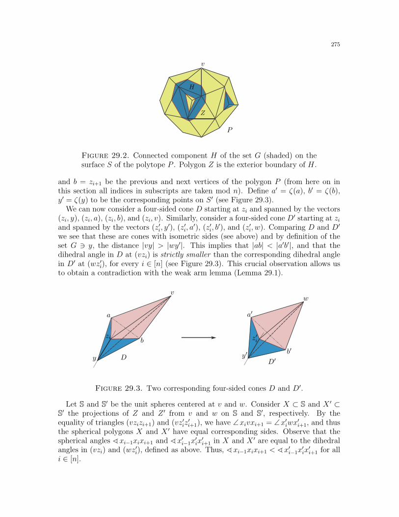
275

v

P

H

Z

Figure 29.2. Connected component H of the set G (shaded) on thesurface S of the polytope P . Polygon Z is the exterior boundary of H .

and b = zi+1 be the previous and next vertices of the polygon P (from here on inthis section all indices in subscripts are taken mod n). Define a′ = ζ(a), b′ = ζ(b),y′ = ζ(y) to be the corresponding points on S ′ (see Figure 29.3).

We can now consider a four-sided cone D starting at zi and spanned by the vectors(zi, y), (zi, a), (zi, b), and (zi, v). Similarly, consider a four-sided cone D′ starting at ziand spanned by the vectors (z′i, y

′), (z′i, a′), (z′i, b

′), and (z′i, w). Comparing D and D′

we see that these are cones with isometric sides (see above) and by definition of theset G ∋ y, the distance |vy| > |wy′|. This implies that |ab| < |a′b′|, and that thedihedral angle in D at (vzi) is strictly smaller than the corresponding dihedral anglein D′ at (wz′i), for every i ∈ [n] (see Figure 29.3). This crucial observation allows usto obtain a contradiction with the weak arm lemma (Lemma 29.1).

v

a

bzi

y

w

a′

b′

z′i

y′DD′

Figure 29.3. Two corresponding four-sided cones D and D′.

Let S and S′ be the unit spheres centered at v and w. Consider X ⊂ S and X ′ ⊂S′ the projections of Z and Z ′ from v and w on S and S′, respectively. By theequality of triangles (vzizi+1) and (vz′iz

′i+1), we have ∠xivxi+1 = ∠x′iwx

′i+1, and thus

the spherical polygons X and X ′ have equal corresponding sides. Observe that thespherical angles ∢xi−1xixi+1 and ∢x′i−1x

′ix

′i+1 in X and X ′ are equal to the dihedral

angles in (vzi) and (wz′i), defined as above. Thus, ∢xi−1xixi+1 < ∢x′i−1x′ix

′i+1 for all

i ∈ [n].

276

Finally, note that X lies in the cone Cv and thus can be moved into an upper hemi-sphere. Similarly, X ′ lies in the cone Cv′ . Since the cone over X ′ with a vertex at w isstrictly smaller than Cv′ , the polygon X ′ also can be moved into an upper hemisphere.By the weak arm lemma (Lemma 29.1), we conclude that such polygons X and X ′

do not exist, a contradiction. This proves that P ≃ Q.

29.3. Killing the monsters. It would be a shame to have a “global” but ratherintricate proof as above, and a rather unexciting inductive proof of the weak armlemma (Lemma 29.1). Fortunately, the fact that the lemma is qualitative rather thanquantitative allows us to create from two polygons a nice imaginary ‘monster’, i.e.,an impossible construction whose nonexistence is easy to establish.

We need a few preliminary definitions and remarks. Let M be a compact metricspace homeomorphic to a sphere. The example to keep in mind is a surface S = ∂Pof a convex body with the distance defined as the length of the shortest path in Sbetween the points. The advantage of the abstract metric spaces is that it can bestudied without an explicit embedding into Euclidean space. Below we use only theabstract spherical polyhedral surfaces (s.p.s.) which are defined by gluing along theedges a finite number of spherical polygons (on a unit sphere S2), such that theresulting manifolds are homeomorphic (but not necessarily isometric) to a sphere.These are analogues of polyhedral surfaces for spherical polyhedra (we will add ananalogue of convexity below). An example is a ‘spherical tetrahedron’ which canbe obtained by gluing together four equilateral spherical triangles with the samesidelength.

Given a s.p.s. M as above, we can define lines, circles, and angles accordingly. Ata point x ∈ M , define the curvature ω(x) = 2π − α(x) where α(x) is the total anglearound x. A point x ∈ S is called flat if ω(x) = 0, and non-flat otherwise. For ak-gon Q ⊂M define

ω(Q) := area(Q) +∑

x∈NF(Q)

ω(x),

where NF(Q) is the set of non-flat interior points x ∈ Q. Using these definitionsone can extend the inductive proof of the Gauss–Bonnet theorem (Theorem 25.3) toobtain that the total curvature of every s.p.s. satisfies ω(M) = 4π.

Finally, we will always assume that our s.p.s. is nonnegatively curved: ω(x) ≥ 0for all x ∈M . Observe that for every two points x, y ∈M we have |xy| ≤ π. Indeed,the shortest path cannot go through points of positive curvature by Proposition 10.1.Thus, every shortest path γ ⊂M between x and y must lie in a flat neighborhood R ⊂M . Since R is isometric to a region in S2 (possibly overlapping), the path γ of length|γ| > π can be shortened. This condition will be important in the proof.

Proof of the weak arm lemma. Let X,X ′ be two spherical polygons as in the lemma.Remove X ′ from a unit sphere S2 and attach X in its place. Denote by M theresulting s.p.s. The only non-flat points in M are the vertices of X = [x1x2 . . . xn].Using notation αi = ∢x′i−1x

′ix

′i+1−∢xi−1xixi+1, we have ω(xi) = αi > 0. Since X ′ is

277

in the upper hemisphere, the s.p.s. M contains a hemisphere B ⊂ S2, and xi ∈MrBfor all i ∈ [n].

Consider a shortest path γ between x1 and x2 and cut M along γ. Let us prove thatthe length |γ| = |x1x2|M < π. Indeed, from above |x1x2| ≤ π. Now, if |x1x2| = π, wecan consider all shortest paths from x1 to x2, and show that they either go throughother points xi, or n = 2, both leading to a contradiction.

Construct two symmetric spherical triangles T1 = [a1a2a3] and T2 = [b1b2b3] on aunit sphere U |a1a2| = |b1b2| = |x1x2|, ∢a2a1a3 = ∢ b2b1b3 = α1/2 and ∢a1a2a3 =∢ b1b2b3 = α2/2. From |x1x2|M < π, for the third angle we have ∢a1a3a2 = ∢ b1b3b2 <π. Glue T1 and T2 to each other: (a1a3) with (b1b3), (a2a3) with (b2b3). Now gluesides (a1a2) and (b1b2) of the triangles to the sides of the cut γ. This gives thenonnegatively curved s.p.s. M1 with only n− 1 non-flat points.

Continue this process to obtain M2,M3, etc., until we obtain Mn−1 with only onenon-flat point y. The complement Mn−1−y is isometric to the complement to a pointof a unit sphere, and has area 4π. Therefore, ω(Mn−1) = 4π + ω(y) > 4π, whichcontradicts the Gauss–Bonnet theorem for s.p.s. (see Exercise 29.1).

Remark 29.2. The condition that the polygons (or at least X ′) are in the upper hemisphereis critical in the weak arm lemma by the same argument as in Section 22.4. Let us see howthis affects the proof above. Consider a sector R on a unit sphere which can be viewed asa 2-gon with vertices x, y at the North and South Pole, and some angle β > 0 between twomeridians. Define M to be a s.p.s. obtained by gluing two sides of A. Now the curvaturein each vertex is ω(x) = ω(y) = 2π − β, while area(R) = 2β. The triangles T1 = T2 havetwo angles (π−β/2) and the third angle is π. Therefore, when we glue R and two trianglestogether we obtain back the sphere S2. As expected, no contradiction in this case.

29.4. Exercises.

Exercise 29.1. (Gauss–Bonnet theorem for s.p.s.) ♦ [1+] State and prove the analogueof the Gauss–Bonnet theorem (Theorem 25.3) for spherical polyhedral surfaces.

Exercise 29.2. [1] Check that the proof above extends verbatim to the proof of the Alexan-drov uniqueness theorem (Theorem 27.7).

Exercise 29.3 (Alexandrov-Sen’kin). [1] Let S, S′ ⊂ R3 be two intrinsically isometricpolyhedral surfaces with the same boundary Q = ∂S = ∂S′. Suppose the origin O isseparated from S, S′ by a hyperplane, and that both S, S′ are seen from O from inside(outside). Then S = S′.

Exercise 29.4. [2-] Modify the proof above to obtain the Pogorelov uniqueness theorem(Theorem 27.8) in the piecewise smooth case.

29.5. Final remarks. The ‘global proof’ of the Cauchy theorem is due to Sen’kin [Sen1]and is not alike any other proof we know. The proof of the weak arm lemma in this sectionfollows a companion paper by Zalgaller [Zal1]. While not as simple as the arm lemma (evenin the corrected version), it is very insightful and brings to light some useful ideas. We referto [BVK] for a slightly expanded presentation of the original proof. The extension of theCauchy theorem in Exercise 29.3 is given in [AS].

278

Interestingly, there seems to be a bit of a tradeoff: the easier the global part is, the harder

the local part is, and vice versa. Pogorelov’s proof in the previous section has a strong local

part, and an easy global part. Similarly, the proof in this section has a reverse emphasis.

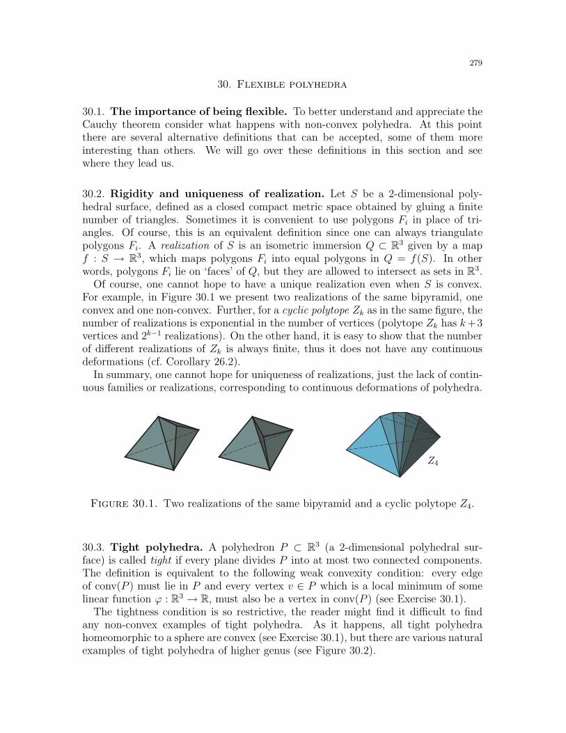
279

30. Flexible polyhedra

30.1. The importance of being flexible. To better understand and appreciate theCauchy theorem consider what happens with non-convex polyhedra. At this pointthere are several alternative definitions that can be accepted, some of them moreinteresting than others. We will go over these definitions in this section and seewhere they lead us.

30.2. Rigidity and uniqueness of realization. Let S be a 2-dimensional poly-hedral surface, defined as a closed compact metric space obtained by gluing a finitenumber of triangles. Sometimes it is convenient to use polygons Fi in place of tri-angles. Of course, this is an equivalent definition since one can always triangulatepolygons Fi. A realization of S is an isometric immersion Q ⊂ R3 given by a mapf : S → R3, which maps polygons Fi into equal polygons in Q = f(S). In otherwords, polygons Fi lie on ‘faces’ of Q, but they are allowed to intersect as sets in R3.

Of course, one cannot hope to have a unique realization even when S is convex.For example, in Figure 30.1 we present two realizations of the same bipyramid, oneconvex and one non-convex. Further, for a cyclic polytope Zk as in the same figure, thenumber of realizations is exponential in the number of vertices (polytope Zk has k+3vertices and 2k−1 realizations). On the other hand, it is easy to show that the numberof different realizations of Zk is always finite, thus it does not have any continuousdeformations (cf. Corollary 26.2).

In summary, one cannot hope for uniqueness of realizations, just the lack of contin-uous families or realizations, corresponding to continuous deformations of polyhedra.

Z4

Figure 30.1. Two realizations of the same bipyramid and a cyclic polytope Z4.

30.3. Tight polyhedra. A polyhedron P ⊂ R3 (a 2-dimensional polyhedral sur-face) is called tight if every plane divides P into at most two connected components.The definition is equivalent to the following weak convexity condition: every edgeof conv(P ) must lie in P and every vertex v ∈ P which is a local minimum of somelinear function ϕ : R3 → R, must also be a vertex in conv(P ) (see Exercise 30.1).

The tightness condition is so restrictive, the reader might find it difficult to findany non-convex examples of tight polyhedra. As it happens, all tight polyhedrahomeomorphic to a sphere are convex (see Exercise 30.1), but there are various naturalexamples of tight polyhedra of higher genus (see Figure 30.2).

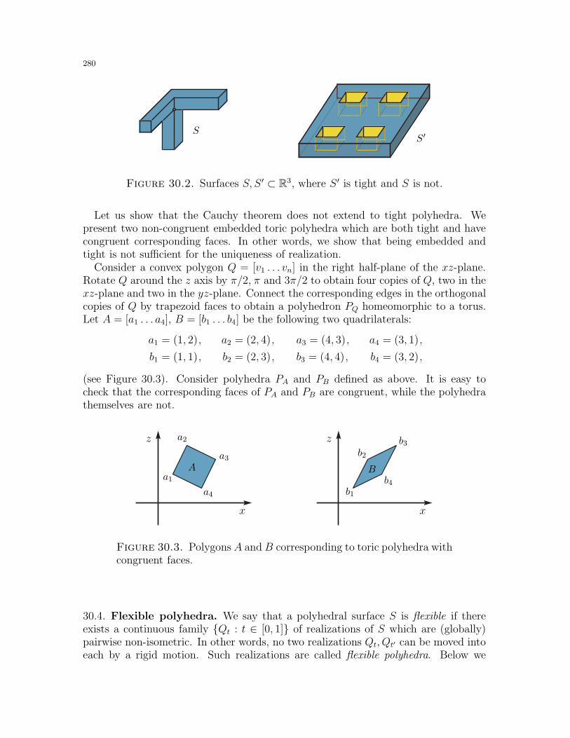
280

S′S

Figure 30.2. Surfaces S, S ′ ⊂ R3, where S ′ is tight and S is not.

Let us show that the Cauchy theorem does not extend to tight polyhedra. Wepresent two non-congruent embedded toric polyhedra which are both tight and havecongruent corresponding faces. In other words, we show that being embedded andtight is not sufficient for the uniqueness of realization.

Consider a convex polygon Q = [v1 . . . vn] in the right half-plane of the xz-plane.Rotate Q around the z axis by π/2, π and 3π/2 to obtain four copies of Q, two in thexz-plane and two in the yz-plane. Connect the corresponding edges in the orthogonalcopies of Q by trapezoid faces to obtain a polyhedron PQ homeomorphic to a torus.Let A = [a1 . . . a4], B = [b1 . . . b4] be the following two quadrilaterals:

a1 = (1, 2), a2 = (2, 4), a3 = (4, 3), a4 = (3, 1),

b1 = (1, 1), b2 = (2, 3), b3 = (4, 4), b4 = (3, 2),

(see Figure 30.3). Consider polyhedra PA and PB defined as above. It is easy tocheck that the corresponding faces of PA and PB are congruent, while the polyhedrathemselves are not.

xx

zz

Aa1

a2

a3

a4

B

b1

b2

b3

b4

Figure 30.3. Polygons A and B corresponding to toric polyhedra withcongruent faces.

30.4. Flexible polyhedra. We say that a polyhedral surface S is flexible if thereexists a continuous family Qt : t ∈ [0, 1] of realizations of S which are (globally)pairwise non-isometric. In other words, no two realizations Qt, Qt′ can be moved intoeach by a rigid motion. Such realizations are called flexible polyhedra. Below we

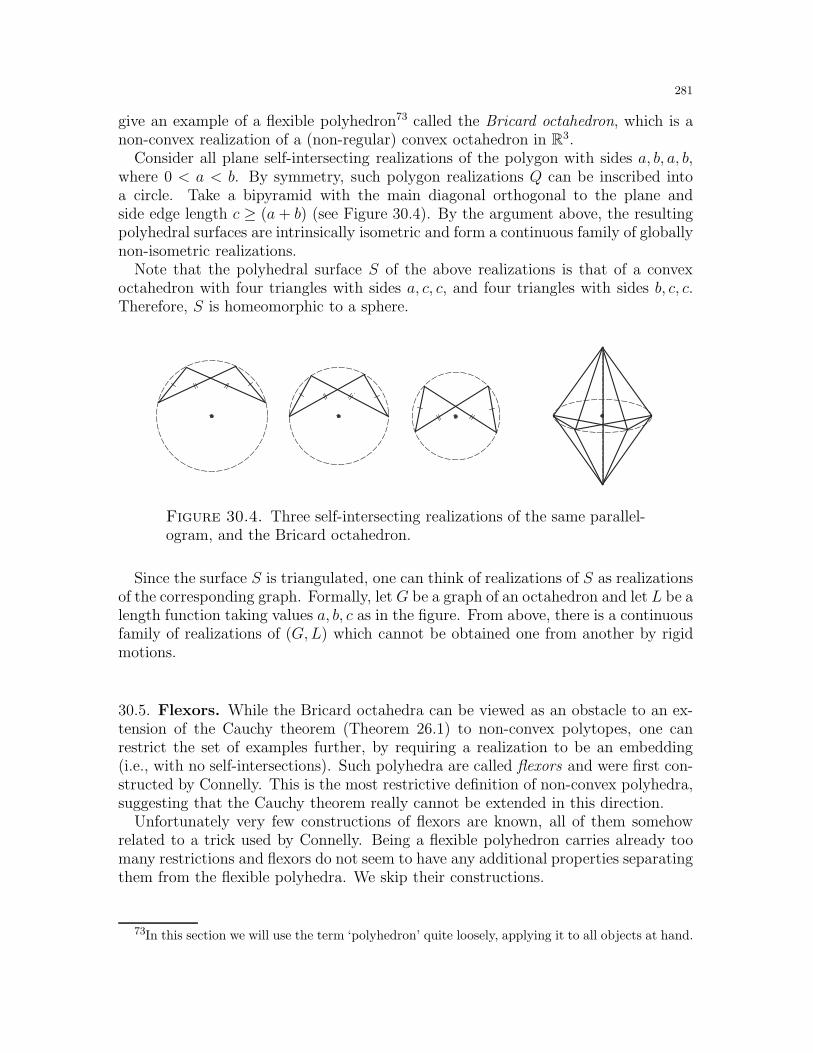
281

give an example of a flexible polyhedron73 called the Bricard octahedron, which is anon-convex realization of a (non-regular) convex octahedron in R3.

Consider all plane self-intersecting realizations of the polygon with sides a, b, a, b,where 0 < a < b. By symmetry, such polygon realizations Q can be inscribed intoa circle. Take a bipyramid with the main diagonal orthogonal to the plane andside edge length c ≥ (a + b) (see Figure 30.4). By the argument above, the resultingpolyhedral surfaces are intrinsically isometric and form a continuous family of globallynon-isometric realizations.

Note that the polyhedral surface S of the above realizations is that of a convexoctahedron with four triangles with sides a, c, c, and four triangles with sides b, c, c.Therefore, S is homeomorphic to a sphere.

Figure 30.4. Three self-intersecting realizations of the same parallel-ogram, and the Bricard octahedron.

Since the surface S is triangulated, one can think of realizations of S as realizationsof the corresponding graph. Formally, let G be a graph of an octahedron and let L be alength function taking values a, b, c as in the figure. From above, there is a continuousfamily of realizations of (G,L) which cannot be obtained one from another by rigidmotions.

30.5. Flexors. While the Bricard octahedra can be viewed as an obstacle to an ex-tension of the Cauchy theorem (Theorem 26.1) to non-convex polytopes, one canrestrict the set of examples further, by requiring a realization to be an embedding(i.e., with no self-intersections). Such polyhedra are called flexors and were first con-structed by Connelly. This is the most restrictive definition of non-convex polyhedra,suggesting that the Cauchy theorem really cannot be extended in this direction.

Unfortunately very few constructions of flexors are known, all of them somehowrelated to a trick used by Connelly. Being a flexible polyhedron carries already toomany restrictions and flexors do not seem to have any additional properties separatingthem from the flexible polyhedra. We skip their constructions.

73In this section we will use the term ‘polyhedron’ quite loosely, applying it to all objects at hand.

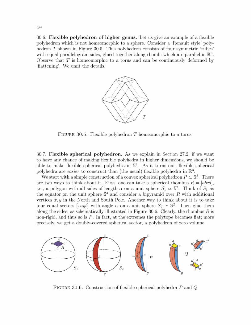
282

30.6. Flexible polyhedron of higher genus. Let us give an example of a flexiblepolyhedron which is not homeomorphic to a sphere. Consider a ‘Renault style’ poly-hedron T shown in Figure 30.5. This polyhedron consists of four symmetric ‘tubes’with equal parallelogram sides, glued together along rhombi which are parallel in R3.Observe that T is homeomorphic to a torus and can be continuously deformed by‘flattening’. We omit the details.

T

Figure 30.5. Flexible polyhedron T homeomorphic to a torus.

30.7. Flexible spherical polyhedron. As we explain in Section 27.2, if we wantto have any chance of making flexible polyhedra in higher dimensions, we should beable to make flexible spherical polyhedra in S3. As it turns out, flexible sphericalpolyhedra are easier to construct than (the usual) flexible polyhedra in R3.

We start with a simple construction of a convex spherical polyhedron P ⊂ S3. Thereare two ways to think about it. First, one can take a spherical rhombus R = [abcd],i.e., a polygon with all sides of length α on a unit sphere S1 ≃ S2. Think of S1 asthe equator on the unit sphere S3 and consider a bipyramid over R with additionalvertices x, y in the North and South Pole. Another way to think about it is to takefour equal sectors [xayb] with angle α on a unit sphere S2 ≃ S2. Then glue themalong the sides, as schematically illustrated in Figure 30.6. Clearly, the rhombus R isnon-rigid, and thus so is P . In fact, at the extremes the polytope becomes flat; moreprecisely, we get a doubly-covered spherical sector, a polyhedron of zero volume.

S1 S2

α

a

a

aa

a

b

b b

bb

b

c

c

c

c

d

d d

d

dxx

yyy

x′

a′

a′

c′

c′

PQ

R

Figure 30.6. Construction of flexible spherical polyhedra P and Q

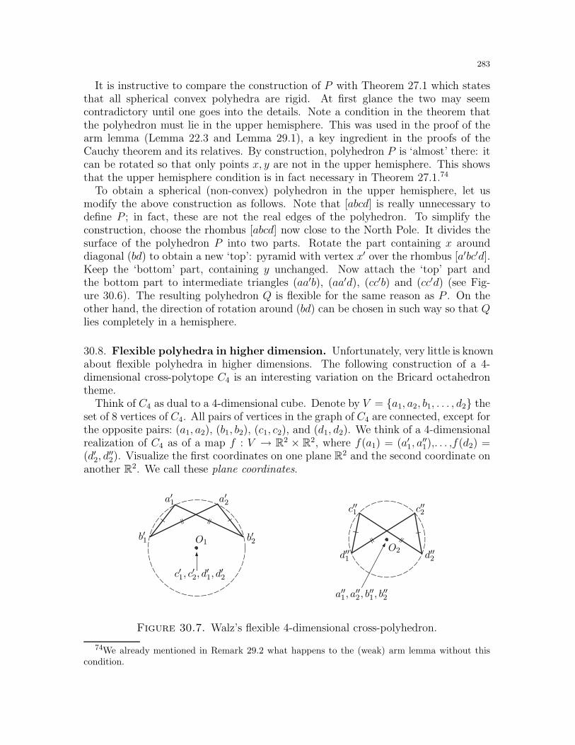
283

It is instructive to compare the construction of P with Theorem 27.1 which statesthat all spherical convex polyhedra are rigid. At first glance the two may seemcontradictory until one goes into the details. Note a condition in the theorem thatthe polyhedron must lie in the upper hemisphere. This was used in the proof of thearm lemma (Lemma 22.3 and Lemma 29.1), a key ingredient in the proofs of theCauchy theorem and its relatives. By construction, polyhedron P is ‘almost’ there: itcan be rotated so that only points x, y are not in the upper hemisphere. This showsthat the upper hemisphere condition is in fact necessary in Theorem 27.1.74

To obtain a spherical (non-convex) polyhedron in the upper hemisphere, let usmodify the above construction as follows. Note that [abcd] is really unnecessary todefine P ; in fact, these are not the real edges of the polyhedron. To simplify theconstruction, choose the rhombus [abcd] now close to the North Pole. It divides thesurface of the polyhedron P into two parts. Rotate the part containing x arounddiagonal (bd) to obtain a new ‘top’: pyramid with vertex x′ over the rhombus [a′bc′d].Keep the ‘bottom’ part, containing y unchanged. Now attach the ‘top’ part andthe bottom part to intermediate triangles (aa′b), (aa′d), (cc′b) and (cc′d) (see Fig-ure 30.6). The resulting polyhedron Q is flexible for the same reason as P . On theother hand, the direction of rotation around (bd) can be chosen in such way so that Qlies completely in a hemisphere.

30.8. Flexible polyhedra in higher dimension. Unfortunately, very little is knownabout flexible polyhedra in higher dimensions. The following construction of a 4-dimensional cross-polytope C4 is an interesting variation on the Bricard octahedrontheme.

Think of C4 as dual to a 4-dimensional cube. Denote by V = a1, a2, b1, . . . , d2 theset of 8 vertices of C4. All pairs of vertices in the graph of C4 are connected, except forthe opposite pairs: (a1, a2), (b1, b2), (c1, c2), and (d1, d2). We think of a 4-dimensionalrealization of C4 as of a map f : V → R2 × R2, where f(a1) = (a′1, a

′′1),. . . ,f(d2) =

(d′2, d′′2). Visualize the first coordinates on one plane R2 and the second coordinate on

another R2. We call these plane coordinates.

a′′1, a′′2 , b

′′1 , b

′′2

c′1, c′2, d

′1, d

′2

O1O2

a′1 a′2

b′1 b′2

c′′1 c′′2

d′′1 d′′2

Figure 30.7. Walz’s flexible 4-dimensional cross-polyhedron.

74We already mentioned in Remark 29.2 what happens to the (weak) arm lemma without thiscondition.

284

Now let the plane coordinates of C4 be as shown in Figure 30.7. Here all planecoordinates either lie on circles or in their centers O1 and O2. Thus, the pairwisedistances between points are either equal to the interval lengths as in the figure, orequal to ℓ =

√ρ2

1 + ρ22, where ρ1, ρ2 are the radii of the circles. Note that both

inscribed 4-gons are flexible, as the circle radii change (compare this with the Bricardoctahedron). Thus, we can keep the distance ℓ constant while changing the radii ofthe circles. Therefore, the above construction gives a flexible polyhedron.

Finally, note that by the argument in Subsection 27.2 every construction of a flexibled-dimensional polyhedron gives several constructions of flexible (d − 1)-dimensionalspherical polyhedra, one per vertex. Of course, in this case all such polyhedra are thespherical analogues of the Bricard octahedron.

30.9. Polyhedral surfaces with boundary. Now that we started expanding theclass of non-convex polyhedra, there is no reason to stop on closed surfaces. Onecan (and, in fact, some people do) consider polyhedral surfaces with boundary. Un-fortunately, in this case flexibility is not an exception but a rule. Basically, if oneremoves two adjacent faces from a surface of a simplicial polytope one obtains aflexible surface:

Theorem 30.1. Let P ⊂ R3 be a simplicial convex polytope, let e be an edge of P ,and let F1, F2 be two faces containing e. Then S := ∂P r (F1 ∪ F2) is a flexiblepolyhedral surface.

Of course, the result cannot be extended to all polytopes. For example, if we removetwo adjacent faces of a cube, the resulting surface is still rigid. The proof of thetheorem is an easy application of the Alexandrov existence theorem (Theorem 37.1),and is presented in Subsection 37.3.

30.10. Exercises.

Exercise 30.1. (Tight polyhedra) ♦ a) [1+] Prove that a polyhedron P ⊂ R3 is tight if andonly if every edge of conv(P ) must lie in P and every vertex v ∈ P which is a (strict) localminimum of some linear function ϕ : R3 → R must be a vertex of conv(P ).b) [1-] Show that neither of the two conditions in a) suffice for the tightness.c) [1-] Check that the two toric polyhedra constructed in Subsection 30.3 are tight.d) [1] Prove that every tight polyhedron embedded into R3 and homeomorphic to a sphereis convex.75

Exercise 30.2. [2-] Generalize to higher dimensions the construction of a toric polyhedronin Subsection 30.6. Check whether they are flexible or rigid.

Exercise 30.3. [1] Consider the Hooker polyhedron defined in the US Patent 3894352.76

Is it flexible or rigid?

Exercise 30.4. a) [∗] Find examples of flexible polyhedra in Rd, for all d ≥ 5.b) [∗] Prove or disprove: every realization of a cross-polytope in R5 is rigid.

75One can view this result as a variation on the convexity criterion given in Exercise 1.25.76See http://www.google.com/patents?vid=USPAT3894352 .

285

30.11. Final remarks. The construction of tight toric polyhedra with isometric faces is dueto Banchoff [Ban1]. See [Kuh] for more on tight polyhedra, generalizations and references.

We refer to [Con2, Con4, FucT] for an introduction to the subject of flexible polyhedraand easy-to-construct examples (see also [Ale4, Dol, Sab5]). Let us note also that Bricardcompletely characterized all flexible octahedra in 1897; there are in fact two additionalfamilies different from the construction we present in this section [Bri2] (see also [Leb3]).We refer to a well written survey [Ale6, §7] for detailed constructions and the references.

Flexible polyhedron homeomorphic to a torus in Subsection 30.6 is one of a large familyof flexible polyhedra introduced by Goldberg [Gol2] (see also [Ale2]). Flexible sphericalpolyhedron in Subsection 30.7 is due to V. A. Alexandrov [Ale3]. Let us mention also thatflexible polyhedra exist in the hyperbolic space H3, where the analogues of the Bricardoctahedra can be proved to be flexible [St2].

The construction in Subsection 30.8 is due to A. Walz (unpublished). Our presentation

follows [St1], where the author gives a more general construction of flexible cross-polytopes.

While no examples of flexible polytopes in higher dimensions are known at the moment,

we do expect the multitude of examples. On the other hand, Stachel conjectured that in

dimension d ≥ 5 there are no flexible cross-polytopes [St1].

286

31. The algebraic approach

The algebraization of realization spaces introduced earlier in the context of linkages(see Section 13) will prove critical to understand the rigidity of non-convex polyhe-dra. In this section we prove Gluck’s theorem and set up a general approach forinfinitesimal rigidity in the next two sections, as well as the bellows conjecture.

31.1. Rigidity vs. flexibility: what is more likely? Let P be a convex polytopeand S = ∂P be its polyhedral surface. The Cauchy theorem states that S is rigid.On the other hand, as the Bricard octahedron and the Connelly polytope show, thisis no longer true for immersions and even for embeddings of S (see the previoussection). The question is what is more likely: that a surface is rigid or flexible?Perhaps unsurprisingly, the answer is unambiguous: a polyhedral (not necessarilyconvex) surface in R3 is almost surely rigid.

We start with the definitions. Let G = (V,E) be a plane triangulation, i.e., a con-nected planar graph with all faces (including exterior face) triangles. Let |V | = n. ByEuler’s formula we have m = |E| = 3n−6 (see Corollary 25.2). Suppose we are givena length function L : E → R+. For each triangle in the plane triangulation G, makea metric triangle with edge lengths given by the length function L. Now glue thesetriangles along the corresponding sides to obtain a simplicial surface S homeomorphicto a sphere.

Clearly, not all length functions define a metric space as the triangle inequalitymust be satisfied. Denote by L(G) the set of all length functions leading to a metricspace. The set L(G) forms a convex cone in Rm with facets corresponding to triangleinequalities for each triangle in G. Denote by L1(G) the set of all length functions L ∈L(G) such that

∑e∈E L(e) ≤ 1. From above, L1(G) is a convex polytope in Rm.

As before, a realization of (G,L) is a map f : V → R3, such that the actual distance∣∣f(v)f(w)∣∣ = L(e) for every edge e = (v, w) ∈ E. Given L ∈ L(G), such a realization

defines an (intrinsically) isometric immersion of S into R3. In the notation above,realizations of (G,L) now correspond to realizations of the surface S.

Finally, rigid motions in R3 act naturally on realizations of (G,L) by acting onsets f(v) | v ∈ V . We are now ready to state the main result.

Theorem 31.1 (Gluck, Poznjak). Let G be a planar triangulation and let L be arandom length function in L1(G). Then, almost surely, (G,L) has only a finite numberof realizations, up to rigid motions.

In other words, the set of non-rigid realizations has measure zero in L(G). Weprove the result by an algebraic argument later in this section.

31.2. The reason why metallic bellows do not exist. The bellows, as any dictio-nary will explain, are mechanical devises which by expansion and contraction pumpair. Basically, these are surfaces which change the volume under bending. Of course,in theory it would be nice to make these surfaces polyhedral, with all faces made outof some kind of metal. In practice this does not work. Here is why (a theoreticalversion).

287

We start with a celebrated bellows conjecture recently resolved by Sabitov. It statesthat the volume of flexible polyhedra is invariant under continuous deformations:

Theorem 31.2 (Former bellows conjecture). Let Qt : t ∈ [0, 1] be a continuousdeformation of a closed polyhedral surface S homeomorphic to a sphere. Then thevolume vol(Qt) is independent of t.

We prove this theorem in Section 34. In fact, the result holds for all closed orientablesurface immersed in R2 (see Subsection 34.7). To illustrate the theorem, note thatthe (signed) volume of the Bricard octahedron and the toric polyhedron T defined inSubsection 30.6, is equal to zero by symmetry. Of course, one can attach a rigid convexpolyhedron to the surface of the either of the two, to obtain a flexible polyhedron ofpositive volume, still constant under flexing.

31.3. Constructing polytopes from scratch. Let P ⊂ R3 be a simplicial convexpolytope with n vertices: V = v1, . . . , vn. For simplicity, let us assume that (v1v2v3)is a face of P . Observe that there always exists a rigid motion which maps vertex v1

into the origin O = (0, 0, 0), v2 into (a, 0, 0), and v3 into (b, c, 0), for some a, b, c ∈ R+.Note also that up to reflection such rigid motion is unique. We call the resultingpolytope planted.

Now, in order to construct a planted polytope from its graph and edge length weneed to set up a system of algebraic (in fact, quadratic) equations. By the Cauchytheorem, there exists only one convex solution, so we are done. Of course, the firstpart of the plan is easy to set up as follows.

Formally, let G = (V,E) be a plane triangulation and let L : E → R+ be a lengthfunction, L ∈ L(G). Denote by f : vi → (xi, yi, zi), i ∈ [n], realizations of (G,L). Forevery pair of vertices (vi, vj) consider a polynomial

Fij := (xi − xj)2 + (yi − yj)2 + (zi − zj)2 .

We consider only planted solutions, i.e., values (x1, . . . , zn) ∈ R3n where

(†) x1 = y1 = z1 = y2 = z2 = z3 = 0.

Denote by R = C[x2, x3, . . . , xn, y3, . . . , yn, z4, . . . , zn] the ring of polynomials on theremaining variables. Now, in the ring R we have the system of equations:

(‡)Fij = (ℓij)

2, for all e = (vi, vj) ∈ E and ℓij = L(e).

As we mentioned before, (‡) is a system of m = 3n − 6 equations with 3n − 6variables. Therefore, if the equations are algebraically independent, we have a finiteset of solutions. The following result positively resolves the problem:

Theorem 31.3 (Gluck). Let G = (V,E) be a plane triangulation. Then polynomi-als Fij corresponding to edges (vi, vj) ∈ E, vi, vj ∈ V , are algebraically independent.

We prove the theorem later in this section. First, let us mention the followingcorollary, which follows easily from the theorem.

288

Corollary 31.4. Under conditions of Theorem 31.3, every polynomial g ∈ R is aroot of a nontrivial algebraic equation:

(⋄) cN tN + . . . + c1 t + c0 = 0,

where cr ∈ C[Fij , (vi, vj) ∈ E], 0 ≤ r ≤ N .

We call polynomial relations (⋄) in the corollary the Sabitov polynomial relations.To obtain the corollary simply note that transcendency degree of R is m = 3n − 6,equal to the number |E| of algebraically independent polynomials Fij in the theorem.

Remark 31.5. (Does this give an algorithm?) It was shown in [FedP] that the degreeof Sabitov polynomials (⋄) is at most 2m and can be exponential even in the most simplecases (see Exercise 31.5). Starting with edge polynomials, one can use standard computeralgebra tools to determine (numerically) the coordinates of all vertices.

31.4. Why polynomials are always better than numbers. Let us continue ourconstruction of the polytope. For each coordinate xi, yi, and zi we need to computethe Sabitov polynomial relations (⋄). Evaluating polynomials Fij at ℓ2ij makes (⋄)into polynomials of the desired values. Compute their roots and try one by one allresulting combinations until a convex one is found.

Alternatively, and more invariantly, we can compute Sabitov polynomials for alldiagonals F1i, F2i and F3i. Again, after their lengths are determined to belong to acertain finite set of solutions, we have a finite number of possibilities to consider.

Now, the above argument clearly contradicts the existence of flexible polyhedra(say, with self-intersections) since it implies that there is always only a finite numberof solutions. The mistake in this argument is very important and may not be obviousat first sight.

. . . . . . [Think about it for a few minutes!] . . . . . .

The mistake is that all polynomial coefficients ci in the Sabitov polynomial rela-tions (⋄) may become zero when evaluated at ℓij. When this happens, we cannotdetermine the corresponding diagonal lengths, thus allowing for the flexible polyhe-dra. On the other hand, if at least one ci 6= 0 in all Sabitov polynomials for diagonalsas above, then there exists only a finite number of planted realizations. In particular,all realizations are (continuously) rigid.

We are now ready to prove Theorem 31.1. First, observe that the polytope L1 oflength functions has full dimension m = 3n− 6 (see next subsection). On the otherhand, for every diagonal (vi, vj), the set of roots of the equation cr = 0 (over R) hascodimension at least 1, where cr is a coefficient of (⋄) corresponding to Fij . Thus,all relations (⋄) are nonzero almost surely, and there exists only a finite number ofrealizations of (G,L), as desired.

Let us think about what is needed to prove Theorem 31.2, the former bellowsconjecture. First, one has to check that vol(P ) is a polynomial in the ring R, i.e.,depends polynomially on the vertex coordinates. Then, by Corollary 31.4 it satisfiesa Sabitov polynomial relation (⋄). If one can prove that the coefficient cN is nonzero,

289

then the volume takes only a finite number of values, and, therefore, remains constantunder continuous deformations. While proving polynomiality of the volume is an easyexercise, checking that cN 6= 0 is a major task; we prove this in Section 34.

31.5. Proof by an algebraic manipulation. Let us first show that Theorem 31.3follows easily from the Cauchy theorem and the Steinitz theorems. The proof is trivialin essence, but requires a good absorbtion of the results and definitions involved.

Proof of Theorem 31.3. Let G = (V,E) be a plane triangulation as in the theorem.Recall that by the Steinitz theorem (Theorem 11.1) there exists a convex polytope Pwith graph G. We can assume that P is planted; otherwise use a rigid motion tomake it so. Perturbing the vertex coordinates of P by < ǫ, while keeping P planted,does not change convexity and the graph of the polytope, for sufficiently small ǫ > 0.By the Cauchy theorem, all perturbations give different length functions L : E → R+

of these realizations of P . In other words, we obtain an open subset X ⊂ Rm ofperturbations of coordinates, each giving a length function L ∈ L(G) ⊂ Rm.

Now consider a characteristic map F = (. . . , Fij, . . .) : Rm → Rm, where Fij willalways correspond to graph edges (vi, vj) ∈ E. The Jacobian J(·) in this case isa determinant of a m × m matrix of partial derivatives of Fij by the coordinates.Since Fij are polynomials, the Jacobian is also a polynomial. From above, J(·) doesnot vanish on an open subsetX ⊂ Rm of the coordinates. Therefore, the Jacobian J(·)is a nontrivial polynomial, and polynomials Fij are algebraically independent.

Remark 31.6. The proof above is based on the Cauchy theorem, but uses a ‘local’ ratherthan a ‘global’ argument. On the other hand, the (continuous) rigidity is insufficient to makethe argument work, since in general the Jacobian can vanish at a point while a polyhedralsurface remains continuously rigid. The examples are given in the previous section. Thiswill also lead us to a notion of static and infinitesimal rigidity which are stronger thancontinuous rigidity, but somewhat easier to prove than the Cauchy theorem.

31.6. Exercises.

Exercise 31.1. [1+] Let P ⊂ R3 be a bipyramid with side length c, over an inscribedn-gon in the plane, with side lengths a. Find a minimal polynomial for the volume of Pwith coefficients in C[a2, c2].

Exercise 31.2. Denote by Qn(a, b) the radius of a convex polygon inscribed into a circlewith n−1 sides a and one side b. Let rn(a, b) be the radius of the this circle, i.e., the radiusof the circle circumscribed around Qn(a, b).a) [1+] Compute a formula for rn(a, b) as a root of a polynomial equation in a2 and b2 interms of the Chebyshev polynomials.b) [1+] Compute the minimal degree of such polynomial relation for rn(a, b).

Exercise 31.3. (Robbins’s problem) Denote by A(a1, . . . , an) and R(a1, . . . , an) the areaand the circumradius of an inscribed convex polygon with sides ai (see Example 34.6 andExercises 34.1, 34.6).a) [1] Prove that A2(·) and R2(·) are algebraic over C[a2

1, . . . , a2n].

290

b) [1+] Prove that in both cases the degrees αn and ρn of the minimal polynomial is atleast Tk when n = 2k + 1, and 2Tk when n = 2k + 2, where Tk is the number of (possiblyself-intersecting) polygons inscribed into a circle.c) [1+] Prove an explicit formula for Tk:

Tk =2k + 1

2

(2k

k

)− 22k−1 .

d) [2] Give an explicit formula for ρn. Check that it proves the upper bound matching thelower bound in b).e) [2] Prove that αn = ρn.

Exercise 31.4. (Connelly’s suspensions) Define a suspension to be a bipyramid over aninscribed polygon (as in Bricard’s octahedron).a) [2] Prove that in every flexible suspension, the inscribed (self-intersecting) polygon musthave each edge length repeated twice, once in each direction.b) [1] Check that such polygons have zero area (cf. Exercise 34.6). Conclude that everyflexible suspension has a zero volume.

Exercise 31.5. (Degrees of Sabitov polynomials) ♦ a) [1] Let Qn denote the bipyramidover an n-gon and let βn be the degree of the Sabitov polynomial of the “main diagonal”.Prove that βn = ρn (see Exercise 31.3). Conclude that βn is exponential.b) [1] Let n denote the degree of Sabitov polynomial of the “main diagonal” in the cyclicpolytope Zn (see Figure 30.1). Prove that n is exponential.c) [2] Use a Bezout type result to show that degrees of Sabitov polynomials (⋄) is at most 2m.

Exercise 31.6. Let ∆ = (v0v1v2v3) ⊂ R3 be a tetrahedron, and let ℓij be its edge lengths,0 ≤ i < j ≤ 3.a) [1-] Find positive values ℓij , 0 ≤ i < j ≤ 3 which satisfy the triangle inequalities

ℓij + ℓjk > ℓik ,

and such that no tetrahedra with these edge lengths exist.b) [1] Consider the set of all possible edge lengths of tetrahedra in R3 :

L = (ℓ01, . . . , ℓ34) ⊂ R6.

Prove that L is not convex.c) [2-] Consider the set of all possible square edge lengths of tetrahedra in R3 :

S = (ℓ201, . . . , ℓ234) ⊂ R6.

Prove that S is convex.

Exercise 31.7. Let ∆ = (v1v2v3v4) ⊂ R3 be a tetrahedron, and let γij denote the dihedralangle at the edge (vi, vj), for all 1 ≤ i < j ≤ 4.a) [1] Prove that γ12 + γ23 + γ34 + γ14 ≤ 2π.b) [1-] Prove that 2π ≤ γ12 + γ13 + γ14 + γ23 + γ24 + γ34 ≤ 3π.c) [1] Prove that 0 ≤ cos γ12 + cos γ13 + cos γ14 + cos γ23 + cos γ24 + cos γ34 ≤ 2.d) [1-] Prove that the second inequality in c) is an equality only if ∆ is equihedral.e) [1+] Show that part a) holds also in the hyperbolic space H3.

291

31.7. Final remarks. Versions of Theorem 31.1 have been proved in much greater gener-ality, e.g., for closed surfaces of every genus. This result is usually attributed to Gluck [Glu],but has also appeared in an earlier paper by Poznjak [Poz].

We prove the bellows conjecture (Theorem 31.2) and give references in Subsection 34.7.To further appreciate Sabitov’s theorem, compare it with the following Connelly’s conjec-ture: In the conditions of Theorem 31.2, polytopes enclosed by Qt are scissor congruent(see [Con2, Con4]). A version of this conjecture was recently disproved in [AleC].

Finally, let us mention that the algebraic approach to the subject and the method of

places recently found unexpected applications to the Robbins’ conjectures (see Exercise 31.3

and 34.6). These conjectures are concerned with properties of polynomial relations on areas

of inscribed convex polygons, as functions of squares of its sides. We refer to [FedP] for

connections between two problems and an algebraic background, and to [Pak4] for a short

survey and further references (see also Exercise 12.3).

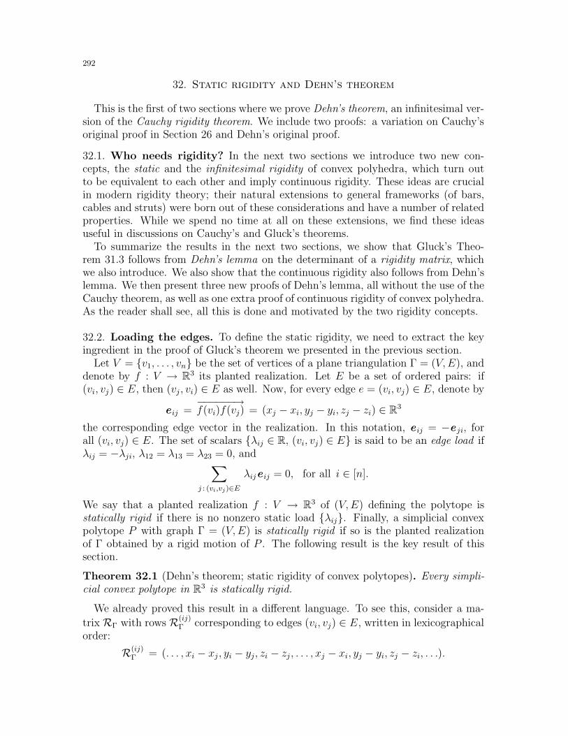
292

32. Static rigidity and Dehn’s theorem

This is the first of two sections where we prove Dehn’s theorem, an infinitesimal ver-sion of the Cauchy rigidity theorem. We include two proofs: a variation on Cauchy’soriginal proof in Section 26 and Dehn’s original proof.

32.1. Who needs rigidity? In the next two sections we introduce two new con-cepts, the static and the infinitesimal rigidity of convex polyhedra, which turn outto be equivalent to each other and imply continuous rigidity. These ideas are crucialin modern rigidity theory; their natural extensions to general frameworks (of bars,cables and struts) were born out of these considerations and have a number of relatedproperties. While we spend no time at all on these extensions, we find these ideasuseful in discussions on Cauchy’s and Gluck’s theorems.

To summarize the results in the next two sections, we show that Gluck’s Theo-rem 31.3 follows from Dehn’s lemma on the determinant of a rigidity matrix, whichwe also introduce. We also show that the continuous rigidity also follows from Dehn’slemma. We then present three new proofs of Dehn’s lemma, all without the use of theCauchy theorem, as well as one extra proof of continuous rigidity of convex polyhedra.As the reader shall see, all this is done and motivated by the two rigidity concepts.

32.2. Loading the edges. To define the static rigidity, we need to extract the keyingredient in the proof of Gluck’s theorem we presented in the previous section.

Let V = v1, . . . , vn be the set of vertices of a plane triangulation Γ = (V,E), anddenote by f : V → R3 its planted realization. Let E be a set of ordered pairs: if(vi, vj) ∈ E, then (vj , vi) ∈ E as well. Now, for every edge e = (vi, vj) ∈ E, denote by

e ij =−−−−−−→f(vi)f(vj) = (xj − xi, yj − yi, zj − zi) ∈ R3

the corresponding edge vector in the realization. In this notation, e ij = −e ji, forall (vi, vj) ∈ E. The set of scalars λij ∈ R, (vi, vj) ∈ E is said to be an edge load ifλij = −λji, λ12 = λ13 = λ23 = 0, and

∑

j : (vi,vj)∈Eλije ij = 0, for all i ∈ [n].

We say that a planted realization f : V → R3 of (V,E) defining the polytope isstatically rigid if there is no nonzero static load λij. Finally, a simplicial convexpolytope P with graph Γ = (V,E) is statically rigid if so is the planted realizationof Γ obtained by a rigid motion of P . The following result is the key result of thissection.

Theorem 32.1 (Dehn’s theorem; static rigidity of convex polytopes). Every simpli-cial convex polytope in R3 is statically rigid.

We already proved this result in a different language. To see this, consider a ma-

trix RΓ with rows R(ij)Γ corresponding to edges (vi, vj) ∈ E, written in lexicographical

order:

R(ij)Γ = (. . . , xi − xj , yi − yj, zi − zj , . . . , xj − xi, yj − yi, zj − zi, . . .).

293

The matrix RΓ is called the rigidity matrix. Now observe, the Jacobian J(·) is adeterminant of the matrix with the following rows:

dFij =

(. . . ,

∂Fij∂xr

,∂Fij∂yr

,∂Fij∂zr

, . . .

)= 2R(ij)

Γ .

We showed that the Jacobian J(·) = 2m detRΓ 6= 0, when evaluated at a plantedrealization f : Γ → R3 defined by a convex polytope P . Thus, there is no nonzerolinear combination of the rows of the rigidity matrix, with coefficients λij as above.Interpreting the set of coefficients λij as the edge load, we obtain the statement ofDehn’s theorem.

In the opposite direction, given Theorem 32.1, we obtain that detRΓ 6= 0. There-fore, the Jacobian is nonzero, which in turn implies Gluck’s theorem without the useof the Cauchy theorem. To conclude this discussion, the static rigidity of convexpolytopes is equivalent to the following technical statement.

Lemma 32.2 (Dehn). Let P ⊂ R3 be a simplicial convex polytope with a graphΓ = (V,E). Then the rigidity matrix RΓ is nonsingular.

In the following two subsections we present three independent proofs of Dehn’slemma, all (hopefully) easier and more elegant than any of the previous proofs of theCauchy theorem. Until then, let us make few more comments.

First, let us show that Dehn’s lemma implies the (continuous) rigidity of convexpolytopes (Corollary 26.7). Indeed, consider the m-dimensional space W of plantedrealizations of Γ = (V,E). The space W is mapped onto the m-dimensional spaceof all length functions, and the determinant J(·) = 2m detRΓ is nonzero at convexrealizations. Therefore, in a small neighborhood of a convex realization the edgelengths are different, and thus a simplicial convex polytope is always rigid.

Our second observation is that the Cauchy theorem is more powerful than Theo-rem 32.1. To see this, recall the Cauchy–Alexandrov theorem on uniqueness of convexpolyhedral surfaces (Theorem 27.6). This immediately implies the rigidity of thesesurfaces77. On the other hand, such realizations are not necessarily statically rigid,as the example in Figure 32.1 shows. Here we make arrows in the directions withpositive coefficients which are written next to the corresponding edges.

32.3. Proof of Dehn’s lemma via sign changes. This proof goes along the verysame lines as the traditional proof of the Cauchy theorem (see Section 26.3). We firstshow that the edge load λij gives a certain assignment of signs on edges, then provethe analogue of the sign changes lemma (Lemma 26.4), and conclude by using thesign counting lemma (Lemma 26.5).

Proof of Dehn’s lemma. Consider an edge load λij | (vi, vj) ∈ E on the edges in P .To remove ubiquity, consider only coefficients λij with i < j. Let us label the edge(vi, vj) ∈ E, i < j, with (+) if λij > 0, with (−) if λij < 0, and with (0) if λij = 0.

77One has to be careful here: this only proves rigidity in the space of convex realizations. In fact,the continuous rigidity holds for all non-strictly convex realizations; this is a stronger result due toConnelly (see [Con5])

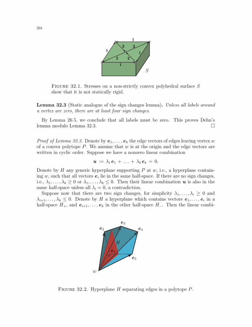
294

1

1

11

22

22

S

Figure 32.1. Stresses on a non-strictly convex polyhedral surface Sshow that it is not statically rigid.

Lemma 32.3 (Static analogue of the sign changes lemma). Unless all labels arounda vertex are zero, there are at least four sign changes.

By Lemma 26.5, we conclude that all labels must be zero. This proves Dehn’slemma modulo Lemma 32.3.

Proof of Lemma 32.3. Denote by e1, . . . , ek the edge vectors of edges leaving vertex wof a convex polytope P . We assume that w is at the origin and the edge vectors arewritten in cyclic order. Suppose we have a nonzero linear combination

u := λ1e1 + . . . + λkek = 0.

Denote by H any generic hyperplane supporting P at w, i.e., a hyperplane contain-ing w, such that all vectors e i lie in the same half-space. If there are no sign changes,i.e., λ1, . . . , λk ≥ 0 or λ1, . . . , λk ≤ 0. Then their linear combination u is also in thesame half-space unless all λi = 0, a contradiction.

Suppose now that there are two sign changes, for simplicity λ1, . . . , λi ≥ 0 andλi+1, . . . , λk ≤ 0. Denote by H a hyperplane which contains vectors e1, . . . , e i in ahalf-space H+, and e i+1, . . . , ek in the other half-space H−. Then the linear combi-

e1

e2

e3

e4

e5

w

H

Figure 32.2. Hyperplane H separating edges in a polytope P .

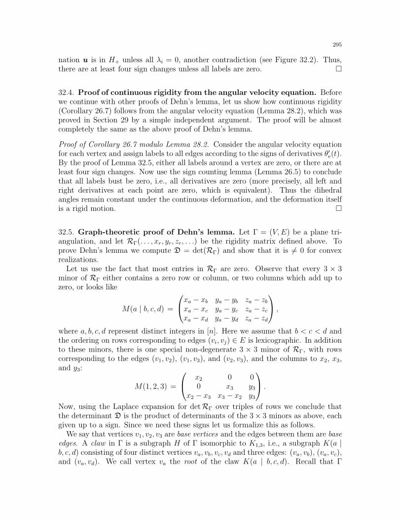
295

nation u is in H+ unless all λi = 0, another contradiction (see Figure 32.2). Thus,there are at least four sign changes unless all labels are zero.

32.4. Proof of continuous rigidity from the angular velocity equation. Beforewe continue with other proofs of Dehn’s lemma, let us show how continuous rigidity(Corollary 26.7) follows from the angular velocity equation (Lemma 28.2), which wasproved in Section 29 by a simple independent argument. The proof will be almostcompletely the same as the above proof of Dehn’s lemma.

Proof of Corollary 26.7 modulo Lemma 28.2. Consider the angular velocity equationfor each vertex and assign labels to all edges according to the signs of derivatives θ′e(t).By the proof of Lemma 32.5, either all labels around a vertex are zero, or there are atleast four sign changes. Now use the sign counting lemma (Lemma 26.5) to concludethat all labels bust be zero, i.e., all derivatives are zero (more precisely, all left andright derivatives at each point are zero, which is equivalent). Thus the dihedralangles remain constant under the continuous deformation, and the deformation itselfis a rigid motion.

32.5. Graph-theoretic proof of Dehn’s lemma. Let Γ = (V,E) be a plane tri-angulation, and let RΓ(. . . , xr, yr, zr, . . .) be the rigidity matrix defined above. Toprove Dehn’s lemma we compute D = det(RΓ) and show that it is 6= 0 for convexrealizations.

Let us use the fact that most entries in RΓ are zero. Observe that every 3 × 3minor of RΓ either contains a zero row or column, or two columns which add up tozero, or looks like

M(a | b, c, d) =

xa − xb ya − yb za − zbxa − xc ya − yc za − zcxa − xd ya − yd za − zd

,

where a, b, c, d represent distinct integers in [n]. Here we assume that b < c < d andthe ordering on rows corresponding to edges (vi, vj) ∈ E is lexicographic. In additionto these minors, there is one special non-degenerate 3 × 3 minor of RΓ, with rowscorresponding to the edges (v1, v2), (v1, v3), and (v2, v3), and the columns to x2, x3,and y3:

M(1, 2, 3) =

x2 0 00 x3 y3

x2 − x3 x3 − x2 y3

.

Now, using the Laplace expansion for detRΓ over triples of rows we conclude thatthe determinant D is the product of determinants of the 3× 3 minors as above, eachgiven up to a sign. Since we need these signs let us formalize this as follows.

We say that vertices v1, v2, v3 are base vertices and the edges between them are baseedges. A claw in Γ is a subgraph H of Γ isomorphic to K1,3, i.e., a subgraph K(a |b, c, d) consisting of four distinct vertices va, vb, vc, vd and three edges: (va, vb), (va, vc),and (va, vd). We call vertex va the root of the claw K(a | b, c, d). Recall that Γ

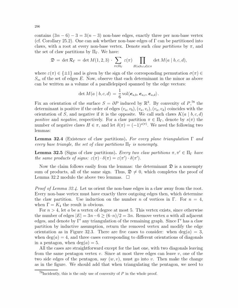
296

contains (3n − 6) − 3 = 3(n − 3) non-base edges, exactly three per non-base vertex(cf. Corollary 25.2). One can ask whether non-base edges of Γ can be partitioned intoclaws, with a root at every non-base vertex. Denote such claw partitions by π, andthe set of claw partitions by ΠΓ. We have:

D = detRΓ = detM(1, 2, 3) ·∑

π∈ΠΓ

ε(π)∏

H(a|b,c,d)∈πdetM(a | b, c, d),

where ε(π) ∈ ±1 and is given by the sign of the corresponding permutation σ(π) ∈Sm of the set of edges E. Now, observe that each determinant in the minor as abovecan be written as a volume of a parallelepiped spanned by the edge vectors:

detM(a | b, c, d) =1

6vol〈ea,b, ea,c, ea,d〉.

Fix an orientation of the surface S = ∂P induced by R3. By convexity of P ,78 thedeterminant is positive if the order of edges (va, vb), (va, vc), (va, vd) coincides with theorientation of S, and negative if it is the opposite. We call such claws K(a | b, c, d)positive and negative, respectively. For a claw partition π ∈ ΠΓ, denote by s(π) thenumber of negative claws H ∈ π, and let δ(π) = (−1)s(π). We need the following twolemmas:

Lemma 32.4 (Existence of claw partitions). For every plane triangulation Γ andevery base triangle, the set of claw partitions ΠΓ is nonempty.

Lemma 32.5 (Signs of claw partitions). Every two claw partitions π, π′ ∈ ΠΓ havethe same products of signs: ε(π) · δ(π) = ε(π′) · δ(π′).

Now the claim follows easily from the lemmas: the determinant D is a nonemptysum of products, all of the same sign. Thus, D 6= 0, which completes the proof ofLemma 32.2 modulo the above two lemmas.

Proof of Lemma 32.4. Let us orient the non-base edges in a claw away from the root.Every non-base vertex must have exactly three outgoing edges then, which determinethe claw partition. Use induction on the number n of vertices in Γ. For n = 4,when Γ = K4 the result is obvious.

For n > 4, let a be a vertex of degree at most 5. This vertex exists, since otherwisethe number of edges |E| = 3n−6 ≥ (6 ·n)/2 = 3n. Remove vertex a with all adjacentedges, and denote by Γ′ any triangulation of the remaining graph. Since Γ′ has a clawpartition by inductive assumption, return the removed vertex and modify the edgeorientation as in Figure 32.3. There are five cases to consider: when deg(a) = 3,when deg(a) = 4, and three cases corresponding to different orientations of diagonalsin a pentagon, when deg(a) = 5.

All the cases are straightforward except for the last one, with two diagonals leavingfrom the same pentagon vertex v. Since at most three edges can leave v, one of thetwo side edges of the pentagon, say (w, v), must go into v. Then make the changeas in the figure. We should add that when triangulating the pentagon, we need to

78Incidently, this is the only use of convexity of P in the whole proof.

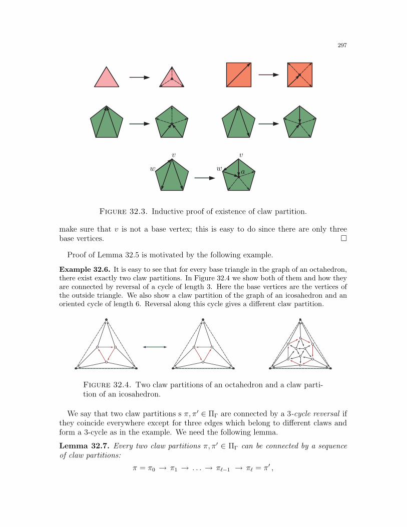
297

ww

vv

a

Figure 32.3. Inductive proof of existence of claw partition.

make sure that v is not a base vertex; this is easy to do since there are only threebase vertices.

Proof of Lemma 32.5 is motivated by the following example.

Example 32.6. It is easy to see that for every base triangle in the graph of an octahedron,there exist exactly two claw partitions. In Figure 32.4 we show both of them and how theyare connected by reversal of a cycle of length 3. Here the base vertices are the vertices ofthe outside triangle. We also show a claw partition of the graph of an icosahedron and anoriented cycle of length 6. Reversal along this cycle gives a different claw partition.

Figure 32.4. Two claw partitions of an octahedron and a claw parti-tion of an icosahedron.

We say that two claw partitions s π, π′ ∈ ΠΓ are connected by a 3-cycle reversal ifthey coincide everywhere except for three edges which belong to different claws andform a 3-cycle as in the example. We need the following lemma.

Lemma 32.7. Every two claw partitions π, π′ ∈ ΠΓ can be connected by a sequenceof claw partitions:

π = π0 → π1 → . . . → πℓ−1 → πℓ = π′ ,

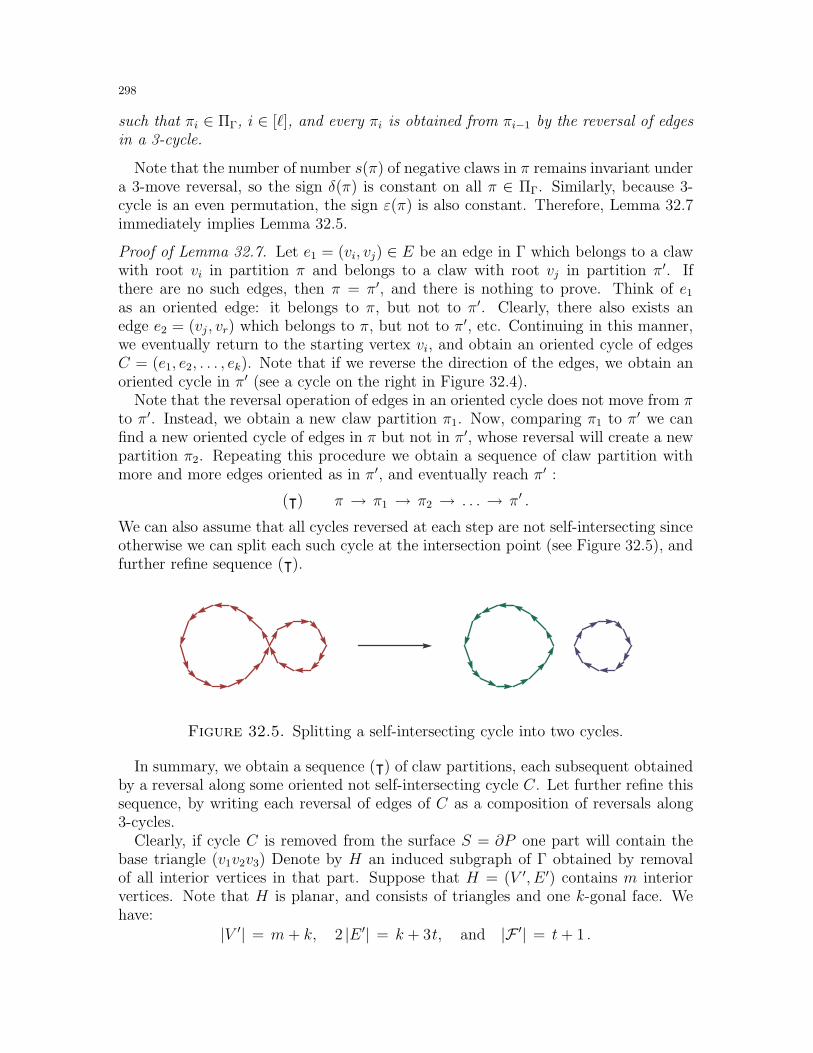
298

such that πi ∈ ΠΓ, i ∈ [ℓ], and every πi is obtained from πi−1 by the reversal of edgesin a 3-cycle.

Note that the number of number s(π) of negative claws in π remains invariant undera 3-move reversal, so the sign δ(π) is constant on all π ∈ ΠΓ. Similarly, because 3-cycle is an even permutation, the sign ε(π) is also constant. Therefore, Lemma 32.7immediately implies Lemma 32.5.

Proof of Lemma 32.7. Let e1 = (vi, vj) ∈ E be an edge in Γ which belongs to a clawwith root vi in partition π and belongs to a claw with root vj in partition π′. Ifthere are no such edges, then π = π′, and there is nothing to prove. Think of e1as an oriented edge: it belongs to π, but not to π′. Clearly, there also exists anedge e2 = (vj , vr) which belongs to π, but not to π′, etc. Continuing in this manner,we eventually return to the starting vertex vi, and obtain an oriented cycle of edgesC = (e1, e2, . . . , ek). Note that if we reverse the direction of the edges, we obtain anoriented cycle in π′ (see a cycle on the right in Figure 32.4).

Note that the reversal operation of edges in an oriented cycle does not move from πto π′. Instead, we obtain a new claw partition π1. Now, comparing π1 to π′ we canfind a new oriented cycle of edges in π but not in π′, whose reversal will create a newpartition π2. Repeating this procedure we obtain a sequence of claw partition withmore and more edges oriented as in π′, and eventually reach π′ :

(⊺) π → π1 → π2 → . . . → π′ .

We can also assume that all cycles reversed at each step are not self-intersecting sinceotherwise we can split each such cycle at the intersection point (see Figure 32.5), andfurther refine sequence (⊺).

Figure 32.5. Splitting a self-intersecting cycle into two cycles.

In summary, we obtain a sequence (⊺) of claw partitions, each subsequent obtainedby a reversal along some oriented not self-intersecting cycle C. Let further refine thissequence, by writing each reversal of edges of C as a composition of reversals along3-cycles.

Clearly, if cycle C is removed from the surface S = ∂P one part will contain thebase triangle (v1v2v3) Denote by H an induced subgraph of Γ obtained by removalof all interior vertices in that part. Suppose that H = (V ′, E ′) contains m interiorvertices. Note that H is planar, and consists of triangles and one k-gonal face. Wehave:

|V ′| = m+ k, 2 |E ′| = k + 3t, and |F ′| = t+ 1 .

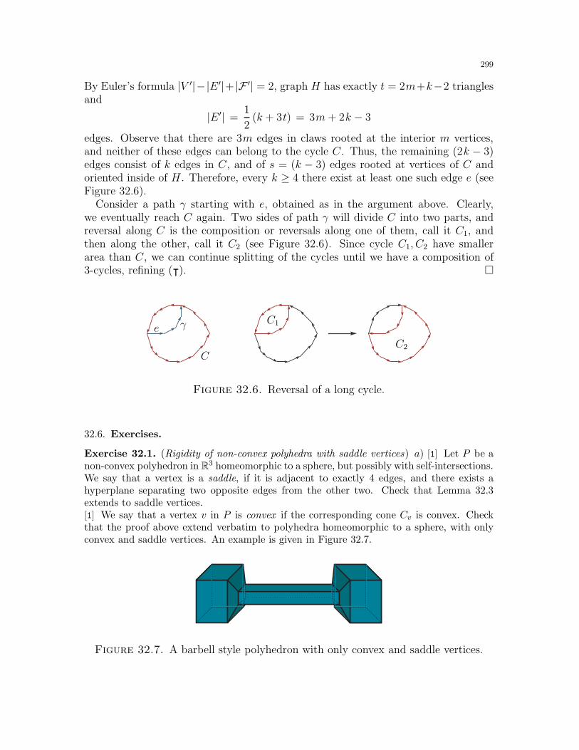
299

By Euler’s formula |V ′|−|E ′|+ |F ′| = 2, graph H has exactly t = 2m+k−2 trianglesand

|E ′| =1

2(k + 3t) = 3m+ 2k − 3

edges. Observe that there are 3m edges in claws rooted at the interior m vertices,and neither of these edges can belong to the cycle C. Thus, the remaining (2k − 3)edges consist of k edges in C, and of s = (k − 3) edges rooted at vertices of C andoriented inside of H . Therefore, every k ≥ 4 there exist at least one such edge e (seeFigure 32.6).

Consider a path γ starting with e, obtained as in the argument above. Clearly,we eventually reach C again. Two sides of path γ will divide C into two parts, andreversal along C is the composition or reversals along one of them, call it C1, andthen along the other, call it C2 (see Figure 32.6). Since cycle C1, C2 have smallerarea than C, we can continue splitting of the cycles until we have a composition of3-cycles, refining (⊺).

e γ

C

C1

C2

Figure 32.6. Reversal of a long cycle.

32.6. Exercises.

Exercise 32.1. (Rigidity of non-convex polyhedra with saddle vertices) a) [1] Let P be anon-convex polyhedron in R3 homeomorphic to a sphere, but possibly with self-intersections.We say that a vertex is a saddle, if it is adjacent to exactly 4 edges, and there exists ahyperplane separating two opposite edges from the other two. Check that Lemma 32.3extends to saddle vertices.[1] We say that a vertex v in P is convex if the corresponding cone Cv is convex. Checkthat the proof above extend verbatim to polyhedra homeomorphic to a sphere, with onlyconvex and saddle vertices. An example is given in Figure 32.7.

Figure 32.7. A barbell style polyhedron with only convex and saddle vertices.

300

Exercise 32.2. [2] Let P ⊂ R3 be a simplicial convex polytope and let S = ∂P . Sup-pose St is a polyhedral deformation which preserves combinatorial structure and dihedralangles. Prove that St is a rigid motion.79

Exercise 32.3. a) [2-] Let P ⊂ R3 be a convex polytope with even-sided faces (quadri-laterals, hexagons, etc.) with surface S = ∂P . Suppose S′ ⊂ R3 is an embedded surfacewhich is combinatorially equivalent to S and whose faces are isometric. Prove that S′ iscontinuously rigid.b) [2-] Extend part a) to polyhedra with at most 7 odd-sided faces.

Exercise 32.4. (Alexandrov) ♦ [1+] Let S = ∂P be a triangulated surface of a convexpolytope P ⊂ R3. Suppose there are no triangle vertices in the relative interior of faces(they are allowed only at vertices and on natural edges of P ). Prove that S is staticallyrigid.

32.7. Final remarks. Dehn’s lemma was used by Dehn [Dehn] to prove Theorem 32.1and deduce from here the continuous rigidity of convex polyhedra (Corollary 26.7). Thisapproach was repeatedly rediscovered and is now only the first basic step in the study ofrigidity of general frameworks. We refer to [Con5, Whi2] for the introduction and a broadoverview of general problems in rigidity theory and various applications.

The static (and thus continuous) rigidity of various families of non-convex polyhedra (seeExercise 32.1) is an interesting part of modern rigidity theory. We refer to surveys [Ale6,Con5] for various references on the subject.

The first proof of Dehn’s lemma (Subsection 32.3) follows [FedP], but can also be foundin the early works on rigidity of frameworks (see [Roth, Whi1]). The proof of continuousrigidity given in Subsection 32.4 is due to Alexandrov [A2, §10.3].

The first part of the graph theoretic proof (Subsection 32.5, until Example 32.6) followsthe original paper of Dehn [Dehn] (see also [Ale6, §6]). The connectivity of all claw partitionsby a sequence of 3-cycle reversals is probably new. The argument here is a variationon theme of several “local move connectivity” arguments (see Subsection 14.7) We referto [KorP] for further discussion on claw partitions of graphs and connections to tilings, andto [Pak3] for a survey on local move connectivity arguments (cf. Section 23).

The extension of the Cauchy and Dehn theorems to polytopes with saddle vertices (asin Exercise 32.1) in fact goes through with many proofs. This result was was proved byStoker [Sto] and then repeatedly rediscovered. Alexandrov’s extension (Exercise 32.4) isthe first step towards Connelly’s theorem on the second order rigidity of all triangulatedconvex surfaces (Exercise 33.5).

Finally, let us note that for small enough angles the argument in the original (incorrect)

proof of the arm lemma (Lemma 22.3) is completely valid. Thus the “incorrect proof” in

fact implies the continuous rigidity of convex polytopes (Corollary 26.2). As we show in this

and the next section, the rigidity of convex polyhedra is somewhat easier to prove than the

uniqueness (the Cauchy theorem). Thus, it is quite tempting to ignore the full power of the

Cauchy theorem, thinking that the continuous rigidity is the most important implication of

uniqueness. From the “real life applications” point of view this idea is actually not without

merits (you really need rigidity, not uniqueness, to prevent a bridge from falling apart).

On the other hand, the proofs of a number of important results, such as the Alexandrov

79This is the infinitesimal version of Stoker’s conjecture for simplicial polytopes.

301

existence theorem (Theorem 37.1), substantially rely on uniqueness. As a consequence, the

full strength of the Cauchy theorem should be neither undervalued nor undermined.

302

33. Infinitesimal rigidity

In this short section we give another approach to the rigidity, and give our ownnew proof of Dehn’s theorem in the previous section.

33.1. You cannot change anything if you do not know how to start. Considera continuous deformation Pt : t ∈ [0, 1] of the simplicial polytope P = P0 ⊂ R3. As

before, let V and E be the set of vertices and edges of P . Denote by v i(t) =−→Ovi the

vector from the origin to the vertex vi = vi(t) of Pt. Think of vectors v′i(t) as velocities

of vertices vi.80 For an edge length |vivj | to be constant under the deformation we

need ‖v i(t) − v j(t)‖′ = 0, where ‖w‖ = (w,w) = |w|2. Thus, in particular, at t = 0we must have:

0 =d

dt

∥∥v i(t)− v j(t)∥∥t=0

=d

dt

∥∥(v i(0)− v j(0))

+ t(v′i(0)− v

′j(0)

)∥∥t=0

= 2(v i(0)− v j(0), v ′

i(0)− v′j(0)

).

This leads to the following natural definition.Let P ⊂ R3 be a planted simplicial polytope. Suppose we are given a vector a i,

for every vertex vi ∈ V . We say that the set of vectors a i defines an infinitesimalrigid motion if

(⊖) (v i − v j,a i − a j) = 0, for every (vi, vj) ∈ E.An infinitesimal rigid motion is called planted if the velocities of base vertices areequal to zero: a1 = a2 = a3 = 0. Finally, we say that a simplicial polytope P ⊂ R3

is infinitesimally rigid if every planted infinitesimal rigid motion is trivial: a i = 0 forall vi ∈ V .

Theorem 33.1 (Dehn’s theorem; infinitesimal rigidity of convex polytopes). Everysimplicial convex polytope in R3 is infinitesimally rigid.

Of course, the restriction to planted infinitesimal rigid motions is necessary, as theusual rigid motions of P in R3 can define nontrivial infinitesimal rigid motions. Also,by definition, the infinitesimal rigidity implies the continuous rigidity.

To prove the theorem, simply observe that infinitesimal rigidity is in fact equivalentto static rigidity, but written from a dual point of view. Indeed, if the determinant D

of the rigidity matrix is nonzero that means that locally all edge lengths of plantedrealizations must be different. Therefore, the space of planted infinitesimal rigidmotions is zero, and vice versa. The details are straightforward.

To summarize, both static and infinitesimal rigidity are equivalent to Dehn’s lemma(Lemma 32.2). In fact, this equivalence extends to general bar frameworks (see [Con5,Whi2]) with no difference in the proof.

80As in Section 28, when the derivatives do not exist we can consider both left and rightderivatives.

303

33.2. A synthetic proof of infinitesimal rigidity. Now, one may ask what isso great about yet another way to rephrase Dehn’s lemma. Well, as it turns out,the infinitesimal rigidity notion is nice enough to allow a graph theoretic approachmarkedly different from the one used above.

The proof we present below yet again splits into two parts: global and local. Thelocal part, while different, has roughly the same level of difficulty as the static analogueof the sign changes lemma (Lemma 32.3). The global part is a simple graph theoreticargument similar in style to the proof of the sign counting lemma (Lemma 26.5).

Proof of Theorem 33.1. First, note that equations (⊖) above say that the differencein the velocity of vertices is orthogonal to the edges of the polytope. Think of ve-locity vectors as vector functions on vertices of P which are equal to 0 on basevertices v1, v2, v3. The idea of the proof is to enlarge the set of such functions andprove a stronger result.

Let V = v1, . . . , vn be the set of vertices of a simplicial convex polytope P ⊂ R3,and let E be the set of edges. Consider the set of all vector sequences (a1, . . . ,an),a i ∈ R3, such that for every edge (vi, vj) ∈ E we have one of the following threepossibilities:

1. (v i − v j,a i) = (v i − v j,a j) = 0,2. (v i − v j,a i) < 0 and (v i − v j ,a j) < 0,3. (v i − v j,a i) > 0 and (v i − v j ,a j) > 0.

In other words, we require that projections of velocity vectors a i and a j onto edge (v i, v j)have the same signs. We say that a vertex vi is dead if a i = 0; it is live otherwise. Weneed to prove that for every vector sequence (a1, . . . ,an) as above, if base verticesare dead, then all vertices vi ∈ V are dead. By definition of infinitesimal rigidity, thiswould immediately imply the theorem.

Denote by Γ = (V,E) the graph of P . Since P is simplicial, Γ is a plane trian-gulation. Consider an orientation edges of Γ in the direction of projections of thevelocity vectors. More precisely, we orient the edge vi → vj in case 2, we orient theedge vi ← vj in case 3, and leave it unoriented vi — vj in case 1.

Consider two edges e = (vi, vj) and e′ = (vi, vr), e, e′ ∈ E, with a common vertex vi,

such that (vi, vj, vr) is a face in P . We say that edges e and e′

have one inversion if one of them is oriented into vi, and the other out of vi, have zero inversions if both of them are oriented into vi or out of vi, have a half-inversion if one of the edges is oriented and the other is unoriented, have one inversion if both of them are unoriented and vi is a live vertex, have zero inversions if both of them are unoriented and vi is a dead vertex.

We say that a triangle is active if at least one of its vertices is live; it is inactiveotherwise. Now consider orientations of an active triangle (vivjvr) where vertex vi islive (see some of them in Figure 33.1). A simple enumeration of all possible casesgives the following result.

Lemma 33.2. Every active triangle has at least one inversion.

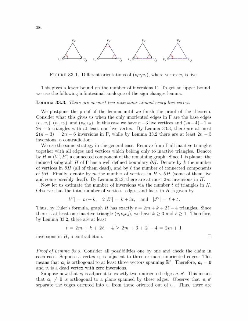
304

vi vi vivivj vj vjvj

vr vr vrvr

Figure 33.1. Different orientations of (vivjvr), where vertex vi is live.

This gives a lower bound on the number of inversions Γ. To get an upper bound,we use the following infinitesimal analogue of the sign changes lemma.

Lemma 33.3. There are at most two inversions around every live vertex.

We postpone the proof of the lemma until we finish the proof of the theorem.Consider what this gives us when the only unoriented edges in Γ are the base edges(v1, v2), (v1, v3), and (v2, v3). In this case we have n−3 live vertices and (2n−4)−1 =2n − 5 triangles with at least one live vertex. By Lemma 33.3, there are at most2(n − 3) = 2n − 6 inversions in Γ, while by Lemma 33.2 there are at least 2n − 5inversions, a contradiction.

We use the same strategy in the general case. Remove from Γ all inactive trianglestogether with all edges and vertices which belong only to inactive triangles. Denoteby H = (V ′, E ′) a connected component of the remaining graph. Since Γ is planar, theinduced subgraph H of Γ has a well defined boundary ∂H . Denote by k the numberof vertices in ∂H (all of them dead), and by ℓ the number of connected componentsof ∂H . Finally, denote by m the number of vertices in H r ∂H (some of them liveand some possibly dead). By Lemma 33.3, there are at most 2m inversions in H .

Now let us estimate the number of inversions via the number t of triangles in H .Observe that the total number of vertices, edges, and faces in H is given by

|V ′| = m+ k, 2 |E ′| = k + 3t, and |F ′| = ℓ+ t .

Thus, by Euler’s formula, graph H has exactly t = 2m+ k + 2ℓ− 4 triangles. Sincethere is at least one inactive triangle (v1v2v3), we have k ≥ 3 and ℓ ≥ 1. Therefore,by Lemma 33.2, there are at least

t = 2m + k + 2ℓ − 4 ≥ 2m + 3 + 2 − 4 = 2m + 1

inversions in H , a contradiction.

Proof of Lemma 33.3. Consider all possibilities one by one and check the claim ineach case. Suppose a vertex vi is adjacent to three or more unoriented edges. Thismeans that a i is orthogonal to at least three vectors spanning R3. Therefore, a i = 0and vi is a dead vertex with zero inversions.

Suppose now that vi is adjacent to exactly two unoriented edges e , e ′. This meansthat a i 6= 0 is orthogonal to a plane spanned by these edges. Observe that e, e ′

separate the edges oriented into vi from those oriented out of vi. Thus, there are

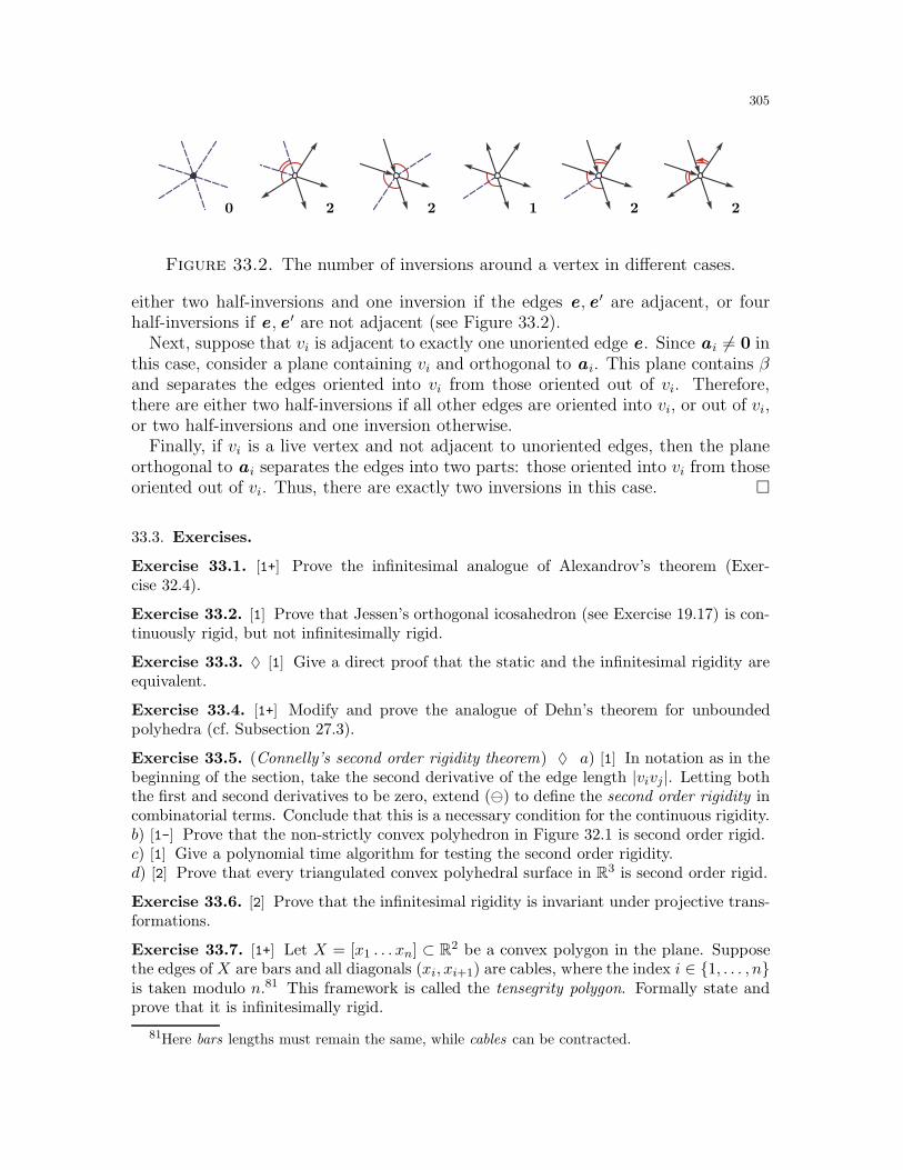
305

0 1 2222

Figure 33.2. The number of inversions around a vertex in different cases.

either two half-inversions and one inversion if the edges e, e ′ are adjacent, or fourhalf-inversions if e , e ′ are not adjacent (see Figure 33.2).

Next, suppose that vi is adjacent to exactly one unoriented edge e. Since a i 6= 0 inthis case, consider a plane containing vi and orthogonal to a i. This plane contains βand separates the edges oriented into vi from those oriented out of vi. Therefore,there are either two half-inversions if all other edges are oriented into vi, or out of vi,or two half-inversions and one inversion otherwise.

Finally, if vi is a live vertex and not adjacent to unoriented edges, then the planeorthogonal to a i separates the edges into two parts: those oriented into vi from thoseoriented out of vi. Thus, there are exactly two inversions in this case.

33.3. Exercises.

Exercise 33.1. [1+] Prove the infinitesimal analogue of Alexandrov’s theorem (Exer-cise 32.4).

Exercise 33.2. [1] Prove that Jessen’s orthogonal icosahedron (see Exercise 19.17) is con-tinuously rigid, but not infinitesimally rigid.

Exercise 33.3. ♦ [1] Give a direct proof that the static and the infinitesimal rigidity areequivalent.

Exercise 33.4. [1+] Modify and prove the analogue of Dehn’s theorem for unboundedpolyhedra (cf. Subsection 27.3).

Exercise 33.5. (Connelly’s second order rigidity theorem) ♦ a) [1] In notation as in thebeginning of the section, take the second derivative of the edge length |vivj|. Letting boththe first and second derivatives to be zero, extend (⊖) to define the second order rigidity incombinatorial terms. Conclude that this is a necessary condition for the continuous rigidity.b) [1-] Prove that the non-strictly convex polyhedron in Figure 32.1 is second order rigid.c) [1] Give a polynomial time algorithm for testing the second order rigidity.d) [2] Prove that every triangulated convex polyhedral surface in R3 is second order rigid.

Exercise 33.6. [2] Prove that the infinitesimal rigidity is invariant under projective trans-formations.

Exercise 33.7. [1+] Let X = [x1 . . . xn] ⊂ R2 be a convex polygon in the plane. Supposethe edges of X are bars and all diagonals (xi, xi+1) are cables, where the index i ∈ 1, . . . , nis taken modulo n.81 This framework is called the tensegrity polygon. Formally state andprove that it is infinitesimally rigid.

81Here bars lengths must remain the same, while cables can be contracted.

306

Exercise 33.8. [1+] Let (x000, x001, . . . , x111) ⊂ R3 be eight vertices corresponding to ver-tices of a cube. Suppose all cube edges, as well as the diagonals in the top and bottom face,are connected by cables. Also, suppose the diagonals in the four side edges are connectedby bars. Prove that this framework is infinitesimally rigid.

Exercise 33.9. Let ∆ = (x1x2x3x4) be a tetrahedron in R3, let ℓij = |xixj |, and let γij bethe dihedral angle at edge (xixj).a) [1] Prove that angles γij determine ∆ uniquely, up to expansion.b) [1] Show that lengths ℓ12, ℓ13, ℓ14 and angles α23, α24, α34 do not necessarily determine ∆.c) [1+] Show that ∆ cannot be continuously deformed so that the angles and lengths in b)remain invariant.

Exercise 33.10. (Rivin, Luo) a) [2+] Let S be an abstract 2-dimensional triangulatedsurface homeomorphic to a sphere, and defined by the edge lengths ℓij = |eij |. Denote byϕij = π − α − β, where α and β are the angles opposite to edge eij . Prove that everycontinuous deformation of S which preserves all ϕij is a homothety.b) [2+] Same result for ϕij = ln(tanα) + ln(tan β).c) [2+] Same result for ϕij = cotα+ cot β.

Exercise 33.11. (Schramm) [2] Suppose two combinatorially equivalent simplicial convexpolyhedra P1, P2 ⊂ R3 have a midscribed sphere, i.e., all their edges touch a fixed unitsphere S2. Suppose further that a face in P1 coincides with the corresponding face in P2.Prove that P1 = P2.

33.4. Final remarks. The synthetic proof of infinitesimal rigidity in this section fol-lows [Pak5] and is based on the proof idea in [Tru]. We refer to [Con5, §4.6] for furtherreferences and other proofs of Dehn’s theorem.

Polyhedra that are continuously but not infinitesimally rigid are called shaky polyhe-dra [Gol4]. Jessen’s orthogonal icosahedron is a classical example of a shaky polyhedron(see Exercises 19.17 and 33.2). A non-strictly convex polyhedron in Figure 32.1 is another,degenerate example.

While continuous rigidity is often hard to establish even for very specific frameworks,

the infinitesimal rigidity is equivalent to a nonzero determinant of the rigidity matrix RΓ.

Similarly, one can define the second and higher order rigidity, which give further necessary

conditions on continuous rigidity (see Exercise 33.5). We refer to [ConS] for the introduction

to higher order rigidity, and to survey papers [Con5, IKS] for further references.

307

34. Proof of the bellows conjecture

We continue the algebraic approach started in Section 31. Here we give a completeproof of the bellows conjecture stated there, modulo some basic algebraic results givenin the Appendix (see Subsection 41.7).

34.1. Polynomiality and integrality of the volume. Let S ⊂ Rd be a polyhedralsurface homeomorphic to a sphere. When S = ∂P is a surface of a convex polytope,we can define the volume enclosed by S as the volume of the polytope P . In general,we can triangulate the surface and define

vol(S) :=1

n!

∑

(v1...vd)∈Sdet[v1, . . . , vd] ,

where (v1 . . . vd) is an oriented simplex in S and det[v1, . . . , vd] is a determinant of amatrix where vi are column-vectors. This implies that the volume of convex polytopesis polynomial in the vertex coordinates.

Now let S = ∂P be the surface of a simplicial convex polytope P ⊂ R3. Its vol-ume is polynomial in vertex coordinates, and by Corollary 31.4 this implies that asa polynomial this volume is a root of an equation with coefficients in C[Fij ], whereFij are polynomials giving the squared distances between vi and vj. In other words,there exists a Sabitov polynomial relation (⋄) for the volume polynomial (see Corol-lary 31.4).

More generally, consider a simplicial surface S ⊂ R3 homeomorphic to a sphere,i.e., a polyhedral surface with only triangular faces. From above, the volume is aroot of a polynomial obtained by an evaluation of the Sabitov polynomial relation (⋄)at the vertex coordinates. Now, as we showed in Section 31, the bellows conjecture(Theorem 31.2) follows immediately if we show that the leading coefficient is 1, orany other nonzero integer, since this implies that the above polynomial does notdegenerate. Let us formalize this property as follows.

Let L be a field which contains a ring R. For our purposes one can always assumethat L is either C or R. We say that an element x ∈ L is integral over R if

xr + cr−1xr−1 + . . . + c1x + c0 = 0.

Now comes the crucial result.

Lemma 34.1 (Integrality of the volume). Let S ⊂ R3 be a simplicial surface homeo-morphic to a sphere and let R be a ring generated by the squares of the edge lengths ℓ2ij.Then 24vol(S) is integral over R.

From above, the lemma implies the bellows conjecture (Theorem 31.2). Its proof isbased on a mixture of algebraic and geometric properties of volume and will occupythe rest of this section.

308

34.2. Playing with infinities. To prove the integrality of the volume we need todevelop some algebraic tools. Below is a quick introduction to the theory of places,which will help resolve the problem.

Let F be a field, and let F = F ∪ ∞. Elements a ∈ F are called finite elements

in F . As before, let L be a field. A map ϕ : L→ F is called a place if ϕ(1) = 1 andit satisfies the following conditions:

(>) ϕ(a± b) = ϕ(a)± ϕ(b), ϕ(a · b) = ϕ(a) · ϕ(b), for all a, b ∈ L.Here it is understood that for all a ∈ F

a±∞ = ∞ ·∞ =1

0= ∞, a

∞ = 0,

and b · ∞ =∞ for all b 6= 0. Furthermore, the expressions

0

0,∞∞ , 0 · ∞, and ∞±∞

are not defined, and the conditions on ϕ do not have to hold in the case when ther.h.s. of (>) is undefined. Note that ϕ(0) = ϕ(1− 1) = ϕ(1)− ϕ(1) = 1− 1 = 0.

For example, take the field of rational Laurent polynomials L = Q(x) and define

a place ϕ : Q(x) → Q by setting ϕ(x) = ∞, ϕ( 1x) = 0, and ϕ(a) = a, for all

a ∈ Q. Viewing the elements f(x) ∈ Q(x) as functions in x defined on R+, have then:ϕ(f) = limx→∞ f(x).

A place ϕ : L → F is called finite on L (on R) if ϕ(a) ∈ F for all a ∈ L (for alla ∈ R). The following standard algebraic result is a key tool in our approach.

Theorem 34.2 (Integrality criterion). Let L be a field containing a ring R. Anelement x ∈ L is integral over R if and only if every place that is finite on R, is alsofinite on x.

Obviously, all elements x ∈ R are integral over R. Note that by the theorem, if xand y are integral over R, then so are −x, x+ y and x · y. On the other hand, evenif x ∈ L, x 6= 0, is integral, then 1/x ∈ L is not necessarily integral. For example, ifL = C and R = Z, then −2,

√2 and i =

√−1 are integral over Z, while 1/2 is not.

34.3. Proof of the bellows conjecture. Just like in several proofs of the Cauchyand Dehn’s theorems, the proof of the bellows conjecture (Theorem 31.2) neatly splitsinto the local and the global part. As before, we first present the global part of theproof, and only then prove the local part.

Proof of Lemma 34.1. Let L = R be the field of vertex coordinates. As in the lemma,denote by R the ring generated by the squared edge lengths. Let F be any fixed field.

Consider a place ϕ : L→ F which is finite on R.Now, let Γ = (V,E) be a graph of the vertices and edges in S. We prove the claim

by induction on the number n = |V | of vertices and the smallest degree of a vertexin Γ. Let us start with the base of induction, which is summarized in the followinglemma, proved later in this section.

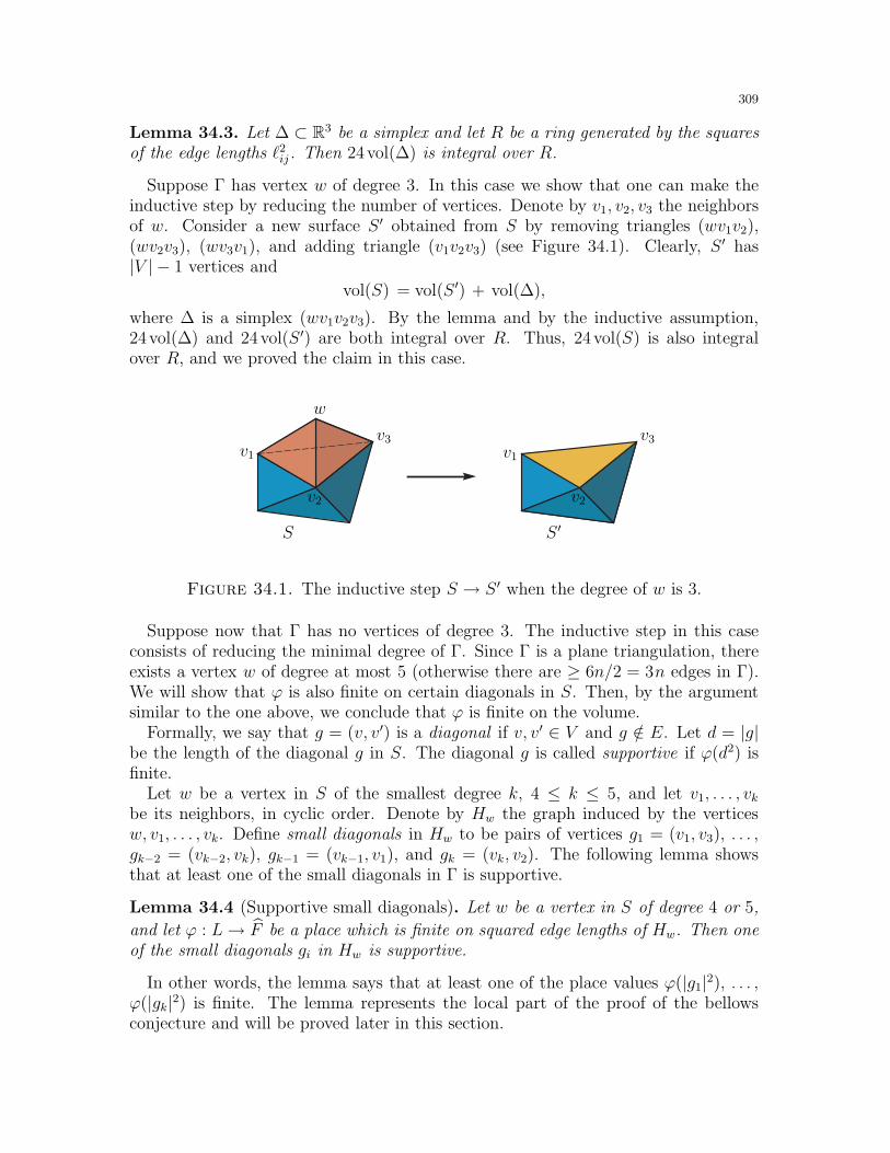
309

Lemma 34.3. Let ∆ ⊂ R3 be a simplex and let R be a ring generated by the squaresof the edge lengths ℓ2ij. Then 24vol(∆) is integral over R.

Suppose Γ has vertex w of degree 3. In this case we show that one can make theinductive step by reducing the number of vertices. Denote by v1, v2, v3 the neighborsof w. Consider a new surface S ′ obtained from S by removing triangles (wv1v2),(wv2v3), (wv3v1), and adding triangle (v1v2v3) (see Figure 34.1). Clearly, S ′ has|V | − 1 vertices and

vol(S) = vol(S ′) + vol(∆),

where ∆ is a simplex (wv1v2v3). By the lemma and by the inductive assumption,24vol(∆) and 24vol(S ′) are both integral over R. Thus, 24vol(S) is also integralover R, and we proved the claim in this case.

S S ′

w

v1 v1

v2 v2

v3 v3

Figure 34.1. The inductive step S → S ′ when the degree of w is 3.

Suppose now that Γ has no vertices of degree 3. The inductive step in this caseconsists of reducing the minimal degree of Γ. Since Γ is a plane triangulation, thereexists a vertex w of degree at most 5 (otherwise there are ≥ 6n/2 = 3n edges in Γ).We will show that ϕ is also finite on certain diagonals in S. Then, by the argumentsimilar to the one above, we conclude that ϕ is finite on the volume.

Formally, we say that g = (v, v′) is a diagonal if v, v′ ∈ V and g /∈ E. Let d = |g|be the length of the diagonal g in S. The diagonal g is called supportive if ϕ(d2) isfinite.

Let w be a vertex in S of the smallest degree k, 4 ≤ k ≤ 5, and let v1, . . . , vkbe its neighbors, in cyclic order. Denote by Hw the graph induced by the verticesw, v1, . . . , vk. Define small diagonals in Hw to be pairs of vertices g1 = (v1, v3), . . . ,gk−2 = (vk−2, vk), gk−1 = (vk−1, v1), and gk = (vk, v2). The following lemma showsthat at least one of the small diagonals in Γ is supportive.

Lemma 34.4 (Supportive small diagonals). Let w be a vertex in S of degree 4 or 5,

and let ϕ : L→ F be a place which is finite on squared edge lengths of Hw. Then oneof the small diagonals gi in Hw is supportive.

In other words, the lemma says that at least one of the place values ϕ(|g1|2), . . . ,ϕ(|gk|2) is finite. The lemma represents the local part of the proof of the bellowsconjecture and will be proved later in this section.

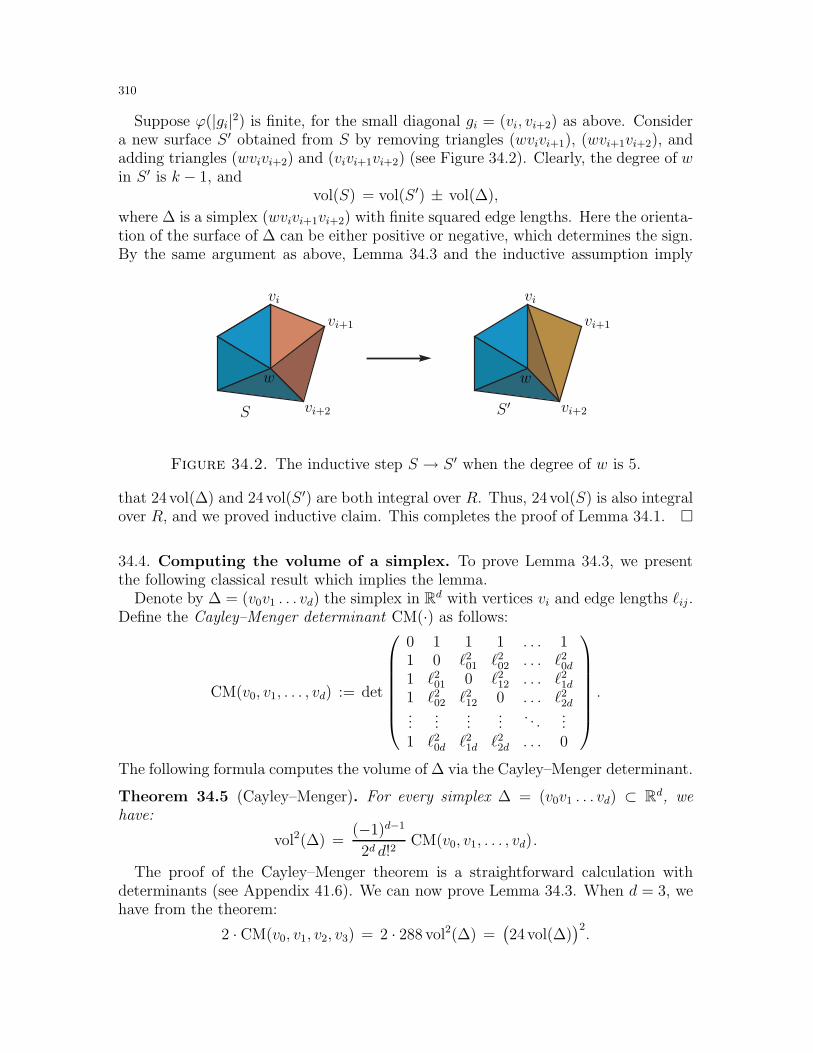
310

Suppose ϕ(|gi|2) is finite, for the small diagonal gi = (vi, vi+2) as above. Considera new surface S ′ obtained from S by removing triangles (wvivi+1), (wvi+1vi+2), andadding triangles (wvivi+2) and (vivi+1vi+2) (see Figure 34.2). Clearly, the degree of win S ′ is k − 1, and

vol(S) = vol(S ′) ± vol(∆),

where ∆ is a simplex (wvivi+1vi+2) with finite squared edge lengths. Here the orienta-tion of the surface of ∆ can be either positive or negative, which determines the sign.By the same argument as above, Lemma 34.3 and the inductive assumption imply

S S ′

w w

vivi

vi+1vi+1

vi+2vi+2

Figure 34.2. The inductive step S → S ′ when the degree of w is 5.

that 24vol(∆) and 24vol(S ′) are both integral over R. Thus, 24vol(S) is also integralover R, and we proved inductive claim. This completes the proof of Lemma 34.1.

34.4. Computing the volume of a simplex. To prove Lemma 34.3, we presentthe following classical result which implies the lemma.

Denote by ∆ = (v0v1 . . . vd) the simplex in Rd with vertices vi and edge lengths ℓij .Define the Cayley–Menger determinant CM(·) as follows:

CM(v0, v1, . . . , vd) := det

0 1 1 1 . . . 11 0 ℓ201 ℓ202 . . . ℓ20d1 ℓ201 0 ℓ212 . . . ℓ21d1 ℓ202 ℓ212 0 . . . ℓ22d...

......

.... . .

...1 ℓ20d ℓ21d ℓ22d . . . 0

.

The following formula computes the volume of ∆ via the Cayley–Menger determinant.

Theorem 34.5 (Cayley–Menger). For every simplex ∆ = (v0v1 . . . vd) ⊂ Rd, wehave:

vol2(∆) =(−1)d−1

2d d!2CM(v0, v1, . . . , vd).

The proof of the Cayley–Menger theorem is a straightforward calculation withdeterminants (see Appendix 41.6). We can now prove Lemma 34.3. When d = 3, wehave from the theorem:

2 · CM(v0, v1, v2, v3) = 2 · 288 vol2(∆) =(24vol(∆)

)2.

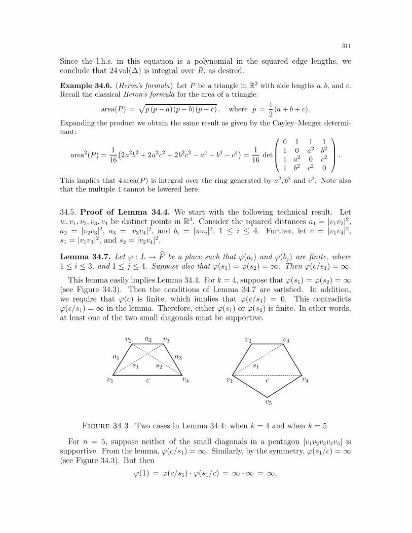
311

Since the l.h.s. in this equation is a polynomial in the squared edge lengths, weconclude that 24vol(∆) is integral over R, as desired.

Example 34.6. (Heron’s formula) Let P be a triangle in R2 with side lengths a, b, and c.Recall the classical Heron’s formula for the area of a triangle:

area(P ) =√p (p − a)(p − b)(p − c) , where p =

1

2(a+ b+ c).

Expanding the product we obtain the same result as given by the Cayley–Menger determi-nant:

area2(P ) =1

16

(2a2b2 + 2a2c2 + 2b2c2 − a4 − b4 − c4

)=

1

16det

0 1 1 11 0 a2 b2

1 a2 0 c2

1 b2 c2 0

.

This implies that 4 area(P ) is integral over the ring generated by a2, b2 and c2. Note alsothat the multiple 4 cannot be lowered here.

34.5. Proof of Lemma 34.4. We start with the following technical result. Letw, v1, v2, v3, v4 be distinct points in R3. Consider the squared distances a1 = |v1v2|2,a2 = |v2v3|2, a3 = |v3v4|2, and bi = |wvi|2, 1 ≤ i ≤ 4. Further, let c = |v1v4|2,s1 = |v1v3|2, and s2 = |v2v4|2.

Lemma 34.7. Let ϕ : L→ F be a place such that ϕ(ai) and ϕ(bj) are finite, where1 ≤ i ≤ 3, and 1 ≤ j ≤ 4. Suppose also that ϕ(s1) = ϕ(s2) =∞. Then ϕ(c/s1) =∞.

This lemma easily implies Lemma 34.4. For k = 4, suppose that ϕ(s1) = ϕ(s2) =∞(see Figure 34.3). Then the conditions of Lemma 34.7 are satisfied. In addition,we require that ϕ(c) is finite, which implies that ϕ(c/s1) = 0. This contradictsϕ(c/s1) =∞ in the lemma. Therefore, either ϕ(s1) or ϕ(s2) is finite. In other words,at least one of the two small diagonals must be supportive.

c cv1 v1

v2 v2v3 v3

v4 v4

v5

a1

a2

a3

s1 s1s2

Figure 34.3. Two cases in Lemma 34.4: when k = 4 and when k = 5.

For n = 5, suppose neither of the small diagonals in a pentagon [v1v2v3v4v5] issupportive. From the lemma, ϕ(c/s1) =∞. Similarly, by the symmetry, ϕ(s1/c) =∞(see Figure 34.3). But then

ϕ(1) = ϕ(c/s1) · ϕ(s1/c) = ∞ ·∞ = ∞,

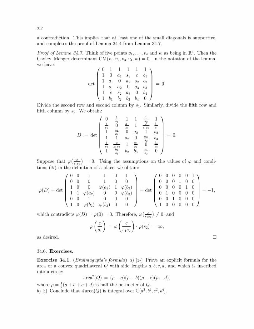
312

a contradiction. This implies that at least one of the small diagonals is supportive,and completes the proof of Lemma 34.4 from Lemma 34.7.

Proof of Lemma 34.7. Think of five points v1, . . . , v4 and w as being in R4. Then theCayley–Menger determinant CM(v1, v2, v3, v4, w) = 0. In the notation of the lemma,we have:

det

0 1 1 1 1 11 0 a1 s1 c b11 a1 0 a2 s2 b21 s1 a2 0 a3 b31 c s2 a3 0 b41 b1 b2 b3 b4 0

= 0.

Divide the second row and second column by s1. Similarly, divide the fifth row andfifth column by s2. We obtain:

D := det

0 1s1

1 1 1s2

11s1

0 a1s1

1 cs1s2

b1s1

1 a1s1

0 a2 1 b21 1 a2 0 a3

s2b3

1s2

cs1s2

1 a3s2

0 b4s2

1 b1s1

b2 b3b4s2

0

= 0.

Suppose that ϕ(

cs1s2

)= 0. Using the assumptions on the values of ϕ and condi-

tions (>) in the definition of a place, we obtain:

ϕ(D) = det

0 0 1 1 0 10 0 0 1 0 01 0 0 ϕ(a2) 1 ϕ(b2)1 1 ϕ(a2) 0 0 ϕ(b3)0 0 1 0 0 01 0 ϕ(b2) ϕ(b3) 0 0

= det

0 0 0 0 0 10 0 0 1 0 00 0 0 0 1 00 1 0 0 0 00 0 1 0 0 01 0 0 0 0 0

= −1,

which contradicts ϕ(D) = ϕ(0) = 0. Therefore, ϕ(

cs1s2

)6= 0, and

ϕ

(c

s1

)= ϕ

(c

s1s2

)· ϕ(s2) = ∞,

as desired.

34.6. Exercises.

Exercise 34.1. (Brahmagupta’s formula) a) [1-] Prove an explicit formula for thearea of a convex quadrilateral Q with side lengths a, b, c, d, and which is inscribedinto a circle:

area2(Q) = (ρ− a)(ρ− b)(ρ− c)(ρ− d),where ρ = 1

2(a+ b+ c+ d) is half the perimeter of Q.

b) [1] Conclude that 4area(Q) is integral over C[a2, b2, c2, d2].

313

Exercise 34.2. a) [1-] Show that a triangle in the plane cannot have odd sides andintegral volume.b) [1] Show that a tetrahedron in R3 cannot have odd edge lengths and integralvolume.c) [1-] Conclude from a) that no 4 points in the plane can have odd pairwise distances.

Exercise 34.3. Two sets A and B of n points are called equivalent if their have thesame multiset of pairwise distances. Similarly, they are called congruent if one canbe obtained from the other by a rigid motion.a) [1] Find two equivalent but non-congruent sets of 4 points in the plane.b) [1+] Show that almost all sets of n ≥ 4 points in the plane have no sets equivalentbut not congruent to them.

Exercise 34.4. ♦ [1] Extend Lemma 34.4 to vertices of degree > 5.

Exercise 34.5. [1+] Let v0, . . . , vd ∈ Rd−1 be any d+ 1 points. Denote by

CM′(v0, v1, . . . , vd) = det(ℓ2ij)

the principal minor of the Cayley–Menger matrix, obtained by removing the first rowand the first column. Prove that CM′(v0, v1, . . . , vd) = 0 if and only if the points lieon a sphere or a hyperplane.

Exercise 34.6. (Robbins problem) Denote by A(a1, . . . , an) the area of a convexpolygon inscribed into a circle with sides ai (cf. Example 34.6, Exercises 13.1, 31.3,and 34.1).a) [1-] Prove that A(·) is a symmetric function.b) [2-] Prove that 4A(·) is integral over C[a2

1, . . . , a2n].

Exercise 34.7. (Extended bellows conjecture) a) [1+] Extend the bellows conjectureto all orientable 2-dimensional polyhedral surfaces in R3. In other words, extendLemma 34.1 to surfaces of any genus.b) [∗] Extend the bellows conjecture to higher dimensions.

Exercise 34.8. (Equiareal triangulations) A dissection of a polygon into triangles ofequal area is called an equiareal triangulation.a) [2] Prove that every equiareal triangulation of a unit square has an odd numberof triangles.b) [2] Suppose a unit square is dissected into triangles with areas a1, . . . , am. Provethat there exists a polynomial f ∈ Z[x1, . . . , xm] such that f(a1, . . . , am) = 1/2.c) [2+] Prove that every equiareal triangulation of a centrally symmetric polygon hasan odd number of triangles.d) [2+] Extend part c) to centrally symmetric polygons of area 1.e) [2] Find a plane quadrilateral which has no equiareal triangulations.f) [2] Find a convex polytope R ⊂ R3 which cannot be dissected into tetrahedra ofequal volume.

314

34.7. Final remarks. The bellows conjecture is usually attributed to Connelly andSullivan (see [Con2]). The idea of finding and studying polynomial relations for thevolume (as in Corollary 31.4) seems to be due to Connelly and Sabitov and goes backto the late 80’s (see [Sab1]). The bellows conjecture, including the case of surfacesof higher genus, was completely resolved by Sabitov in a series of papers of varyingdifficulty [Sab2, Sab3, Sab4]. Our presentation is based on [CSW], where the ideaof using the theory of places has been introduced. This approach was later usedby Connelly to give a simple proof of one of the Robbins conjectures [Con6] (seeExercise 34.6 and [Pak4]). We refer to [Schl3] for for more on the background of theconjecture and the proof.

The bellows conjecture remains open in higher dimensions (see Exercise 34.7).It is known to hold for the few available examples of flexible polyhedra (see Sub-section 30.8). Interestingly, the bellows conjecture fails for spherical polyhedra, asexhibited by a flexible spherical polyhedron given in Subsection 30.7 (see [Ale3]). Anumber of counterexamples to the infinitesimal versions of the conjecture was givenin [Ale1]. Finally, the conjecture remains open for hyperbolic polyhedra (see [Ale6]for the references).

The theory of places is often presented as part of a more general theory of valua-tions. In this context the integrality criterion (Theorem 34.2) is called the Chevalleyextension lemma (see [Cohn, §9.1]) and is usually stated in terms of valuation rings(see [AtiM, Corollary 5.22] and [Mats, Theorem 10.4]).

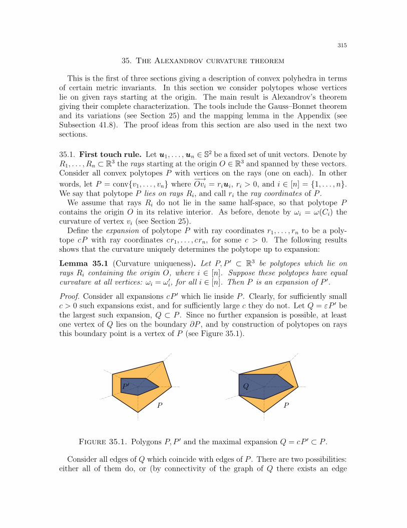
315

35. The Alexandrov curvature theorem

This is the first of three sections giving a description of convex polyhedra in termsof certain metric invariants. In this section we consider polytopes whose verticeslie on given rays starting at the origin. The main result is Alexandrov’s theoremgiving their complete characterization. The tools include the Gauss–Bonnet theoremand its variations (see Section 25) and the mapping lemma in the Appendix (seeSubsection 41.8). The proof ideas from this section are also used in the next twosections.

35.1. First touch rule. Let u1, . . . ,un ∈ S2 be a fixed set of unit vectors. Denote byR1, . . . , Rn ⊂ R3 the rays starting at the origin O ∈ R3 and spanned by these vectors.Consider all convex polytopes P with vertices on the rays (one on each). In other

words, let P = convv1, . . . , vn where−→Ovi = riu i, ri > 0, and i ∈ [n] = 1, . . . , n.

We say that polytope P lies on rays Ri, and call ri the ray coordinates of P .We assume that rays Ri do not lie in the same half-space, so that polytope P

contains the origin O in its relative interior. As before, denote by ωi = ω(Ci) thecurvature of vertex vi (see Section 25).

Define the expansion of polytope P with ray coordinates r1, . . . , rn to be a poly-tope cP with ray coordinates cr1, . . . , crn, for some c > 0. The following resultsshows that the curvature uniquely determines the polytope up to expansion:

Lemma 35.1 (Curvature uniqueness). Let P, P ′ ⊂ R3 be polytopes which lie onrays Ri containing the origin O, where i ∈ [n]. Suppose these polytopes have equalcurvature at all vertices: ωi = ω′

i, for all i ∈ [n]. Then P is an expansion of P ′.

Proof. Consider all expansions cP ′ which lie inside P . Clearly, for sufficiently smallc > 0 such expansions exist, and for sufficiently large c they do not. Let Q = εP ′ bethe largest such expansion, Q ⊂ P . Since no further expansion is possible, at leastone vertex of Q lies on the boundary ∂P , and by construction of polytopes on raysthis boundary point is a vertex of P (see Figure 35.1).

P P

P ′ Q

Figure 35.1. Polygons P, P ′ and the maximal expansion Q = cP ′ ⊂ P .

Consider all edges of Q which coincide with edges of P . There are two possibilities:either all of them do, or (by connectivity of the graph of Q there exists an edge

316

e = (vi, vj) in Q, with one vertex vi in P and the other vertex vj in the interiorof P . In the first case, all vertices of Q coincide with those in P and polytope Pis an expansion of P ′. In the second case, denote by Ci the cone spanned by edgesof P starting at vi, and by Di the cone spanned by edges of Q starting at v′i. Then,by construction, Ci ⊃ Di and Ci 6= Di. Therefore, by the monotonicity of the conecurvature (Exercise 25.5), we have ωi = ω(Ci) < ω(Di) = ω′

i, a contradiction.

35.2. Inequalities on curvatures. Before we can state the converse of Lemma 35.1,we need to give the necessary conditions on the curvatures.

As before, let P be a convex polytope which lies on rays Ri, which do not lie inthe same half-space, and let ωi > 0 be the curvatures of the vertices, i ∈ [n]. First,recall the Gauss–Bonnet theorem (Theorem 25.3):

ω1 + . . . + ωn = 4π.

In addition, there is a number of inequalities given by the geometry of rays.

Lemma 35.2. For a subset I ⊂ [n], denote by CI = convRi : i ∈ I the convexcone spanned by the rays. Assume CI 6= R3. Then

∑k/∈I ωk > ω(CI).

Proof. Let P ′ be a convex polyhedron obtained as a convex hull of P and rays Ri,for all i ∈ [n]. Since CI 6= R3, polyhedron P ′ is well defined. Note that the verticesof P ′ are given by vk /∈ CI , so in particular, k /∈ I. Since O is a point in the relativeinterior of P , the cones of P and P ′ at all such vertices vk satisfy Ck ⊂ C ′

k. Bythe monotonicity of the cone curvature (Exercise 25.5), we have ω′

k ≤ ωk, and theinequality is strict for vertices of unbounded faces of C ′

k. Applying Theorem 25.5 topolyhedron P ′, we obtain:

∑

k/∈Iωk >

∑

k/∈Iω′k ≥

∑

k∈[n] : vk /∈CI

ω′k = ω(CI),

as desired.

35.3. Inequalities on ray coordinates. Let us now describe the set of ray coordi-nates of all convex polytopes which lie on given rays R1, . . . , Rn. As it turns out, it isconvenient to use the inverse ray coordinates. Formally, let xi = 1

riand let X denote

the set of all (x1, . . . , xn) ∈ Rn, such that xi > 0 and(

1x1, . . . , 1

xn

)are ray coordinates

of a polytope on rays Ri.

Lemma 35.3. Suppose R1, . . . , Rn ⊂ R3 are rays which do not lie in the same half-space. Then set X of inverse ray coordinates is an open convex cone in Rn.

Proof. Since all polytopes P which lie on rays Ri must contain the origin, their combi-natorics is completely determined as follows. For every three independent rays Ra, Rb

and Rc, consider a cone C = Ca,b,c spanned by these rays. Whenever ray Ri liesinside C, the vertex vi of Ri must be separated from O by a plane H spanned by va, vband vc.

317

As before, let ua,u b,uc and u i be the unit vectors along the rays. Suppose

u i = αua + βu b + γuc .

We immediately have

riu i = ri (αua + βu b + γuc) =

(riα

ra

)raua +

(riβ

rb

)rbu b +

(riγ

rc

)rcu c .

Observe that the plane H consists of points λava+λbvb+λcvc, for all λa+λb+λc = 1,and let s > 0 be defined by

s ·(α

ra+

β

rb+

γ

rc

)= 1.

Therefore, vertex vi lies on H whenever ri = s and vi is separated from O by H ifri > s. Rewriting the last inequality in the inverse ray coordinates xi = 1

riwe obtain

xi < αxa + βxb + γxc. Taking the intersection of these halfspaces for all cones C asabove, with the halfspaces xi > 0, we obtain convex cone X as in the lemma.

35.4. Finding polytopes with given curvatures. We are ready now to prove themain result of this section. For a subset I ⊂ [n], denote by CI = convRi : i ∈ Ithe convex cone spanned by the rays.

Theorem 35.4 (Alexandrov curvature theorem). Suppose R1, . . . , Rn ⊂ R3 are rayswhich do not lie in the same half-space, and suppose ω1, . . . , ωn ∈ R satisfy the fol-lowing conditions:

1) ωi > 0, for all i ∈ [n],2) ω1 + . . . + ωn = 4π,3)∑

k/∈I ωk > ω(CI), for every I ⊂ [n], such that CI 6= R3.

Then, up to expansion, there exists a unique convex polytope P ⊂ R3 which lies onrays Ri and has curvatures ωi at vertices vi ∈ Ri, for all i ∈ [n]. Conversely, allcurvatures ωi of such polytopes P must satisfy conditions 1)– 3).

One can think of this theorem as both the extension and the converse of Lemma 35.1.Of course, the second part follows from Lemma 35.2 and the Gauss-Bonnet theorem.

Remark 35.5. Let us first check that this result is plausible. There are n − 1 degrees

of freedom of the ray coordinates modulo expansion. This matches the n − 1 degrees of

freedom of the vertex curvatures modulo the Gauss–Bonnet formula. Therefore, by the

curvature uniqueness theorem and the inverse function theorem, for small perturbations

of ωi, there is always a small perturbation of the ray coordinates ri giving these curvatures.

The following proof uses a variation on the same argument.

Proof of Theorem 35.4. Let X ⊂ Rn be the cone of inverse ray coordinates xi, and letX be the intersection of X with a hyperplane defined by x1 + . . .+ xn = 1. Clearly,X is an open (n− 1)-dimensional convex polytope. Also, for every polytope P withinverse ray coordinates x ∈ X , there is a unique c > 0 and an expansion cP withinverse ray coordinates cx ∈ X.

318

Denote by Θ ⊂ Rn the set of all w = (ω1, . . . , ωn) as in the theorem. Denote byϕ : X → Θ the map defined by ϕ(x ) = w , where x = (x1, . . . , xn). By Lemma 35.2,the curvatures satisfy three conditions in the theorem, so this map is well defined.We now deduce the result from the mapping lemma (Theorem 41.8). First, both Xand Θ are open connected manifolds of the same dimension n− 1. By Lemma 35.1,map ϕ is injective. Obviously, map ϕ is continuous. It remains to show that ϕ isproper.

Suppose w k → w as k → ∞, where w k,w ∈ Θ. Assume wk = ϕ(x k) for somex k ∈ X . Since X is a bounded convex polytope, the sequence x k has a convergingsubsequence to some point x ∈ Rn. We need to show that x ∈ X . Denote by Pk thepolytopes corresponding to x k. By contradiction, if x /∈ X , then it lies on one of thefacets, i.e., either xi = αxa + βxb + γxc for some i, a, b, c ∈ [n], or xi = 0 for somei ∈ [n], in notation of the proof of Lemma 35.3. In the first case, the limit of Pi is anon-strictly convex polytope P where vertex vi lies in the plane spanned by (vavbvc).But then the limit of the curvatures ωi in w k is 0, a contradiction with w ∈ Θ.

In the second case, if xi = 1ri→ 0, we have ri → ∞, and the limit polyhedron

Pk → P is unbounded. Let us first show that P is well defined. Denote by I the setof all i ∈ [n] such that ri → ∞. By convexity, this implied that the same holds forall i ∈ [n] such that Ri ⊂ CI . Thus, if CI = R3 we have xi →→ 0 for all i ∈ [n], acontradiction with x1 + . . . + xn = 1. Therefore, polyhedron P is well defined andcontains only those rays Ri, s.t. i ∈ I. In other words, the base cone CP coincideswith the cone CI . Applying Theorem 25.5 to P , we have

∑j /∈I ωj = ω(CP ) = ω(CI),

a contradiction with w ∈ Θ. This finishes the proof that ϕ is proper. By the mappinglemma, ϕ is a homeomorphism, which proves the result.

35.5. Convex cap curvatures. Let H ⊂ R3 be a plane, which we always think ashorizontal. Fix n points a1, . . . , an ∈ H in general position, i.e., such that no threeof them lie on a line. Consider lines Li⊥H , such that ai ∈ Li, for all i ∈ [n]. Forconvenience, assume that the origin O is in the interior of conva1, . . . , an. Considera convex cap P ⊂ R3 with vertices vi ∈ Li and the base cone CP a ray orthogonalto H and pointing down.

One can ask if there is a way to characterize the curvatures ωi of vertices of convexcaps. Of course, shifting the convex cap P up by a fixed constant does not change thecurvatures. Also, by the Gauss–Bonnet theorem for convex caps (see Section 25.5),we have ω1 + . . .+ ωn = 2π. As the following theorem shows, there are no nontrivialinequalities on the curvatures.

Theorem 35.6 (Alexandrov curvature theorem for convex caps). Fix a plane Hin R3 and lines L1, . . . , Ln ⊂ R3 orthogonal to H. Suppose ω1, . . . , ωn > 0 satisfyω1 + . . .+ωn = 2π. Then, up to translation, there exists a unique convex cap P whichlies on lines Li and has curvatures ωi at vertices vi ∈ Ri, for all i ∈ [n].

There is a topological proof (using the mapping lemma) of this theorem which weleave to the reader (Exercise 35.2). Below we present a variational principle argumentproving a stronger result (see the reduction in Exercise 35.5).

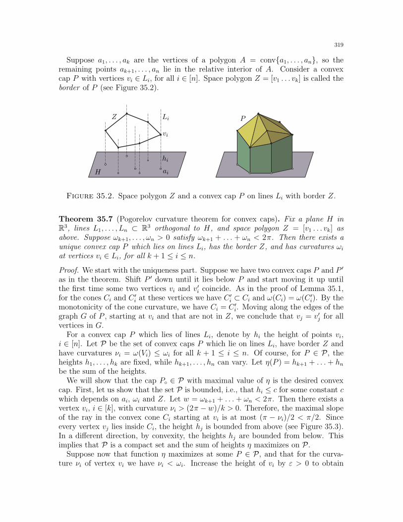
319

Suppose a1, . . . , ak are the vertices of a polygon A = conva1, . . . , an, so theremaining points ak+1, . . . , an lie in the relative interior of A. Consider a convexcap P with vertices vi ∈ Li, for all i ∈ [n]. Space polygon Z = [v1 . . . vk] is called theborder of P (see Figure 35.2).

PLiZ

ai

vi

H

hi

Figure 35.2. Space polygon Z and a convex cap P on lines Li with border Z.

Theorem 35.7 (Pogorelov curvature theorem for convex caps). Fix a plane H inR3, lines L1, . . . , Ln ⊂ R3 orthogonal to H, and space polygon Z = [v1 . . . vk] asabove. Suppose ωk+1, . . . , ωn > 0 satisfy ωk+1 + . . . + ωn < 2π. Then there exists aunique convex cap P which lies on lines Li, has the border Z, and has curvatures ωiat vertices vi ∈ Li, for all k + 1 ≤ i ≤ n.

Proof. We start with the uniqueness part. Suppose we have two convex caps P and P ′

as in the theorem. Shift P ′ down until it lies below P and start moving it up untilthe first time some two vertices vi and v′i coincide. As in the proof of Lemma 35.1,for the cones Ci and C ′

i at these vertices we have C ′i ⊂ Ci and ω(Ci) = ω(C ′

i). By themonotonicity of the cone curvature, we have Ci = C ′

i. Moving along the edges of thegraph G of P , starting at vi and that are not in Z, we conclude that vj = v′j for allvertices in G.

For a convex cap P which lies of lines Li, denote by hi the height of points vi,i ∈ [n]. Let P be the set of convex caps P which lie on lines Li, have border Z andhave curvatures νi = ω(Vi) ≤ ωi for all k + 1 ≤ i ≤ n. Of course, for P ∈ P, theheights h1, . . . , hk are fixed, while hk+1, . . . , hn can vary. Let η(P ) = hk+1 + . . .+ hnbe the sum of the heights.

We will show that the cap P ∈ P with maximal value of η is the desired convexcap. First, let us show that the set P is bounded, i.e., that hi ≤ c for some constant cwhich depends on ai, ωi and Z. Let w = ωk+1 + . . . + ωn < 2π. Then there exists avertex vi, i ∈ [k], with curvature νi > (2π − w)/k > 0. Therefore, the maximal slopeof the ray in the convex cone Ci starting at vi is at most (π − νi)/2 < π/2. Sinceevery vertex vj lies inside Ci, the height hj is bounded from above (see Figure 35.3).In a different direction, by convexity, the heights hj are bounded from below. Thisimplies that P is a compact set and the sum of heights η maximizes on P.

Suppose now that function η maximizes at some P ∈ P, and that for the curva-ture νi of vertex vi we have νi < ωi. Increase the height of vi by ε > 0 to obtain

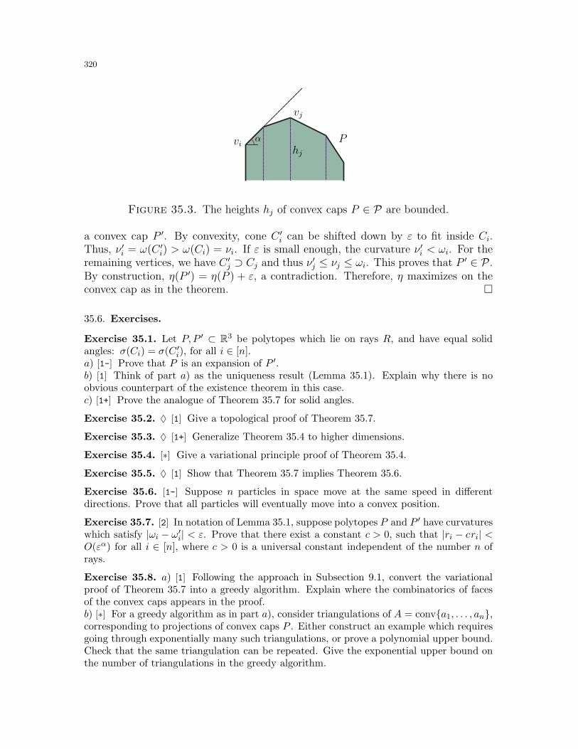
320

Pαvi

vj

hj

Figure 35.3. The heights hj of convex caps P ∈ P are bounded.

a convex cap P ′. By convexity, cone C ′i can be shifted down by ε to fit inside Ci.

Thus, ν ′i = ω(C ′i) > ω(Ci) = νi. If ε is small enough, the curvature ν ′i < ωi. For the

remaining vertices, we have C ′j ⊃ Cj and thus ν ′j ≤ νj ≤ ωi. This proves that P ′ ∈ P.

By construction, η(P ′) = η(P ) + ε, a contradiction. Therefore, η maximizes on theconvex cap as in the theorem.

35.6. Exercises.

Exercise 35.1. Let P,P ′ ⊂ R3 be polytopes which lie on rays R, and have equal solidangles: σ(Ci) = σ(C ′

i), for all i ∈ [n].a) [1-] Prove that P is an expansion of P ′.b) [1] Think of part a) as the uniqueness result (Lemma 35.1). Explain why there is noobvious counterpart of the existence theorem in this case.c) [1+] Prove the analogue of Theorem 35.7 for solid angles.

Exercise 35.2. ♦ [1] Give a topological proof of Theorem 35.7.

Exercise 35.3. ♦ [1+] Generalize Theorem 35.4 to higher dimensions.

Exercise 35.4. [∗] Give a variational principle proof of Theorem 35.4.

Exercise 35.5. ♦ [1] Show that Theorem 35.7 implies Theorem 35.6.

Exercise 35.6. [1-] Suppose n particles in space move at the same speed in differentdirections. Prove that all particles will eventually move into a convex position.

Exercise 35.7. [2] In notation of Lemma 35.1, suppose polytopes P and P ′ have curvatureswhich satisfy |ωi − ω′

i| < ε. Prove that there exist a constant c > 0, such that |ri − cri| <O(εα) for all i ∈ [n], where c > 0 is a universal constant independent of the number n ofrays.

Exercise 35.8. a) [1] Following the approach in Subsection 9.1, convert the variationalproof of Theorem 35.7 into a greedy algorithm. Explain where the combinatorics of facesof the convex caps appears in the proof.b) [∗] For a greedy algorithm as in part a), consider triangulations of A = conva1, . . . , an,corresponding to projections of convex caps P . Either construct an example which requiresgoing through exponentially many such triangulations, or prove a polynomial upper bound.Check that the same triangulation can be repeated. Give the exponential upper bound onthe number of triangulations in the greedy algorithm.

321

Exercise 35.9. Let (ω1, . . . , ωn), satisfy n ≥ 4, 0 < ωi < 2π, for all 1 ≤ i ≤ n, andω1 + . . . + ωn = 4π.a) [2-] Prove that there exists a convex polytope P ⊂ R3 with n vertices, which hascurvatures ωi, 1 ≤ i ≤ n.b) [2-] Suppose n is even. Prove that there exists a simple polytope P ⊂ R3 with n vertices,which has curvatures ωi, 1 ≤ i ≤ n.

Exercise 35.10. ♦ a) [1] Find a collection of rays Ri as in Theorem 35.4, such that thenumber of different cones CI is exponential.b) [∗] Prove or disprove: deciding whether condition 3) is satisfied for given R1, . . . , Rn ∈ R3

and ω1, . . . , ωn > 0, is NP-hard.

Exercise 35.11. ♦ [1] In notation of the mapping lemma (Theorem 41.8), suppose Aand B are connected, but ϕ is only locally injective: for every b ∈ B we have ϕ(a1) = ϕ(a2)implies a1 = a2 in a sufficiently small neighborhood of b. Prove the analogue of the mappinglemma in this case.

35.7. Final remarks. The curvature existence theorem (Theorem 35.4) is due to Alexan-drov and our proof follows [A2]. Both Theorem 35.6 and 35.7 follow from Alexandrov’smost general result. The version with the border Z and the variational principle proof inSubsection 35.5 is due to Pogorelov (see [Pog3, §2.4]).

To explain the motivation behind the results in this section, consider the history of theproblem. Let f : B → R be a convex function defined on a convex region B ⊂ R2. Thinkof points sb = (b, f(b)), where b ∈ B as forming a convex surface S ⊂ R3. Followingthe Cauchy problem, one can ask whether for given boundary values f : ∂B → R andthe curvature function σ : b → σ(sb), one can reconstruct the surface S? Note here thelogic in the question: the curvature is a fundamentally local parameter, so we are askingwhether such local parameter can determine a global structure of the surface. This problemwas resolved by Alexandrov in a much more general form. Theorem 35.7 is both a simplespecial case and an important lemma in the proof.

Now, one ask a similar question for the surfaces of general convex bodies in R3. Here thecurvature is defined not on a plane but on a unit sphere, via spherical projections. This caseis more technical because of the inequalities as in Lemma 35.2. Again, this was resolved byAlexandrov in full generality. Theorem 35.4 corresponds to the case of convex polytopes,when the curvature is concentrated in the vertices.

Recall that prior to this section, we proved a number of uniqueness and rigidity resultson convex polyhedra, including the Cauchy and Dehn rigidity theorems, as well as theirvariations and generalizations. In the next two sections we give two more existence results.One can think of this section as a gate to the next two sections.

Namely, the Minkowski theorem (Theorem 36.2) on existence and uniqueness of convexpolytopes with given normals and areas of the faces. Informally one can think of thisresult as dual to Theorem 36.2. As the reader shall see, we use an unusual variational typeargument to prove this result, and a “first touch rule” analogue for unbounded polyhedra.Similarly, for the Alexandrov existence theorem (Theorem 37.1) we give a topological proofbased on the mapping lemma. In fact, the proof uses Lemma 35.3.

Let us note also that while the existence is often harder and more delicate to establish

(as in this section), the uniqueness results play an important role in classical Differential

Geometry (see Subsection 38.5).

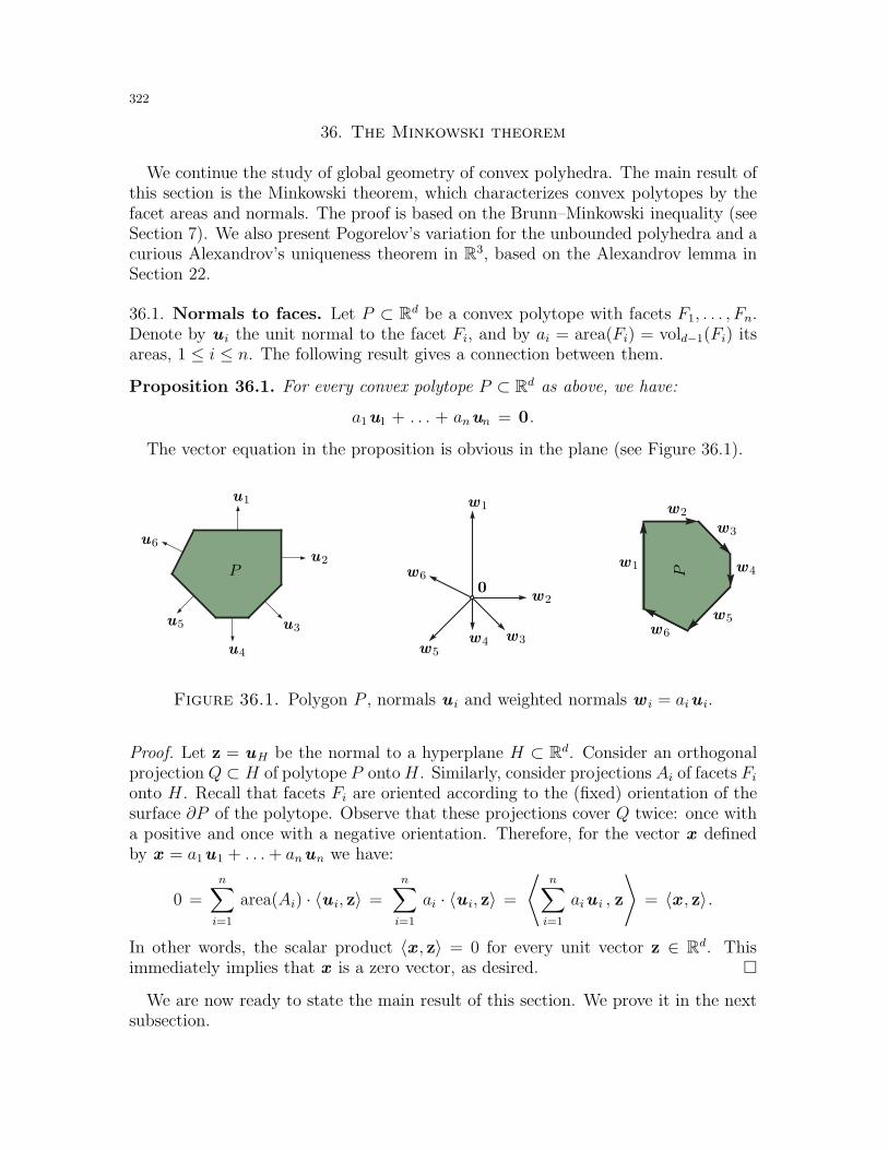
322

36. The Minkowski theorem

We continue the study of global geometry of convex polyhedra. The main result ofthis section is the Minkowski theorem, which characterizes convex polytopes by thefacet areas and normals. The proof is based on the Brunn–Minkowski inequality (seeSection 7). We also present Pogorelov’s variation for the unbounded polyhedra and acurious Alexandrov’s uniqueness theorem in R3, based on the Alexandrov lemma inSection 22.

36.1. Normals to faces. Let P ⊂ Rd be a convex polytope with facets F1, . . . , Fn.Denote by u i the unit normal to the facet Fi, and by ai = area(Fi) = vold−1(Fi) itsareas, 1 ≤ i ≤ n. The following result gives a connection between them.

Proposition 36.1. For every convex polytope P ⊂ Rd as above, we have:

a1u1 + . . . + anun = 0.

The vector equation in the proposition is obvious in the plane (see Figure 36.1).

w1

w1

w6

w6

w5

w5

w4

w4

w3

w3

w2

w2

PP

u1

u6

u5

u4

u3

u2

0

Figure 36.1. Polygon P , normals u i and weighted normals w i = aiu i.

Proof. Let z = uH be the normal to a hyperplane H ⊂ Rd. Consider an orthogonalprojection Q ⊂ H of polytope P ontoH . Similarly, consider projections Ai of facets Fionto H . Recall that facets Fi are oriented according to the (fixed) orientation of thesurface ∂P of the polytope. Observe that these projections cover Q twice: once witha positive and once with a negative orientation. Therefore, for the vector x definedby x = a1u1 + . . .+ anun we have:

0 =

n∑

i=1

area(Ai) · 〈u i, z〉 =

n∑

i=1

ai · 〈u i, z〉 =

⟨n∑

i=1

aiu i , z

⟩= 〈x , z〉.

In other words, the scalar product 〈x , z〉 = 0 for every unit vector z ∈ Rd. Thisimmediately implies that x is a zero vector, as desired.

We are now ready to state the main result of this section. We prove it in the nextsubsection.

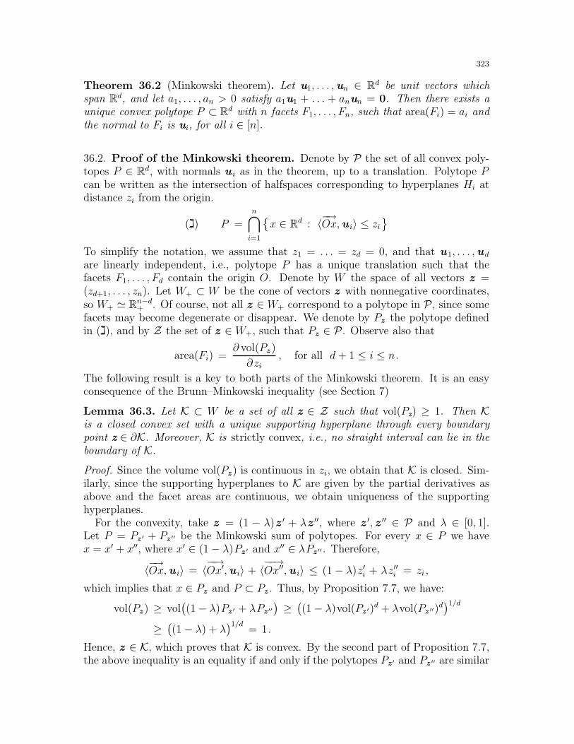
323

Theorem 36.2 (Minkowski theorem). Let u1, . . . ,un ∈ Rd be unit vectors whichspan Rd, and let a1, . . . , an > 0 satisfy a1u1 + . . . + anun = 0. Then there exists aunique convex polytope P ⊂ Rd with n facets F1, . . . , Fn, such that area(Fi) = ai andthe normal to Fi is ui, for all i ∈ [n].

36.2. Proof of the Minkowski theorem. Denote by P the set of all convex poly-topes P ∈ Rd, with normals u i as in the theorem, up to a translation. Polytope Pcan be written as the intersection of halfspaces corresponding to hyperplanes Hi atdistance zi from the origin.

(ג) P =n⋂

i=1

x ∈ Rd : 〈−→Ox,u i〉 ≤ zi

To simplify the notation, we assume that z1 = . . . = zd = 0, and that u1, . . . ,ud

are linearly independent, i.e., polytope P has a unique translation such that thefacets F1, . . . , Fd contain the origin O. Denote by W the space of all vectors z =(zd+1, . . . , zn). Let W+ ⊂ W be the cone of vectors z with nonnegative coordinates,so W+ ≃ Rn−d+ . Of course, not all z ∈W+ correspond to a polytope in P, since somefacets may become degenerate or disappear. We denote by Pz the polytope definedin ,(ג) and by Z the set of z ∈W+, such that Pz ∈ P. Observe also that

area(Fi) =∂ vol(Pz )

∂zi, for all d+ 1 ≤ i ≤ n.

The following result is a key to both parts of the Minkowski theorem. It is an easyconsequence of the Brunn–Minkowski inequality (see Section 7)

Lemma 36.3. Let K ⊂ W be a set of all z ∈ Z such that vol(Pz) ≥ 1. Then Kis a closed convex set with a unique supporting hyperplane through every boundarypoint z ∈ ∂K. Moreover, K is strictly convex, i.e., no straight interval can lie in theboundary of K.

Proof. Since the volume vol(Pz ) is continuous in zi, we obtain that K is closed. Sim-ilarly, since the supporting hyperplanes to K are given by the partial derivatives asabove and the facet areas are continuous, we obtain uniqueness of the supportinghyperplanes.

For the convexity, take z = (1 − λ)z ′ + λz ′′, where z′, z ′′ ∈ P and λ ∈ [0, 1].

Let P = Pz ′ + Pz ′′ be the Minkowski sum of polytopes. For every x ∈ P we havex = x′ + x′′, where x′ ∈ (1− λ)Pz ′ and x′′ ∈ λPz ′′. Therefore,

〈−→Ox,u i〉 = 〈−−→Ox′,u i〉 + 〈

−−→Ox′′,u i〉 ≤ (1− λ)z′i + λz′′i = zi ,

which implies that x ∈ Pz and P ⊂ Pz . Thus, by Proposition 7.7, we have:

vol(Pz ) ≥ vol((1− λ)Pz ′ + λPz ′′

)≥((1− λ)vol(Pz ′)d + λvol(Pz ′′)d

)1/d

≥((1− λ) + λ

)1/d= 1.

Hence, z ∈ K, which proves that K is convex. By the second part of Proposition 7.7,the above inequality is an equality if and only if the polytopes Pz ′ and Pz ′′ are similar

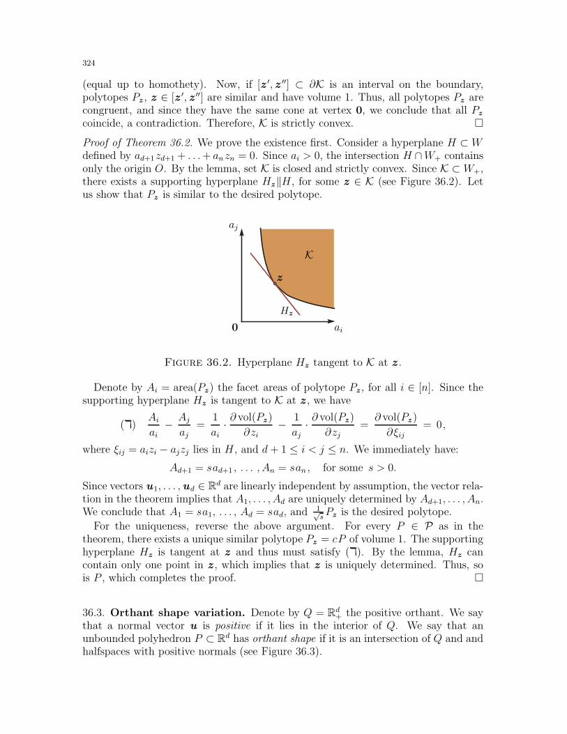
324

(equal up to homothety). Now, if [z ′, z ′′] ⊂ ∂K is an interval on the boundary,polytopes Pz , z ∈ [z ′, z ′′] are similar and have volume 1. Thus, all polytopes Pz arecongruent, and since they have the same cone at vertex 0, we conclude that all Pz

coincide, a contradiction. Therefore, K is strictly convex.

Proof of Theorem 36.2. We prove the existence first. Consider a hyperplane H ⊂Wdefined by ad+1zd+1 + . . .+ anzn = 0. Since ai > 0, the intersection H ∩W+ containsonly the origin O. By the lemma, set K is closed and strictly convex. Since K ⊂W+,there exists a supporting hyperplane Hz‖H , for some z ∈ K (see Figure 36.2). Letus show that Pz is similar to the desired polytope.

0 ai

aj

z

K

Hz

Figure 36.2. Hyperplane Hz tangent to K at z .

Denote by Ai = area(Pz ) the facet areas of polytope Pz , for all i ∈ [n]. Since thesupporting hyperplane Hz is tangent to K at z , we have

(k)Aiai− Aj

aj=

1

ai· ∂ vol(Pz )

∂zi− 1

aj· ∂ vol(Pz )

∂zj=

∂ vol(Pz )

∂ξij= 0,

where ξij = aizi − ajzj lies in H , and d+ 1 ≤ i < j ≤ n. We immediately have:

Ad+1 = sad+1 , . . . , An = san , for some s > 0.

Since vectors u1, . . . ,ud ∈ Rd are linearly independent by assumption, the vector rela-tion in the theorem implies that A1, . . . , Ad are uniquely determined by Ad+1, . . . , An.We conclude that A1 = sa1, . . . , Ad = sad, and 1√

sPz is the desired polytope.

For the uniqueness, reverse the above argument. For every P ∈ P as in thetheorem, there exists a unique similar polytope Pz = cP of volume 1. The supportinghyperplane Hz is tangent at z and thus must satisfy (k). By the lemma, Hz cancontain only one point in z , which implies that z is uniquely determined. Thus, sois P , which completes the proof.

36.3. Orthant shape variation. Denote by Q = Rd+ the positive orthant. We saythat a normal vector u is positive if it lies in the interior of Q. We say that anunbounded polyhedron P ⊂ Rd has orthant shape if it is an intersection of Q and andhalfspaces with positive normals (see Figure 36.3).

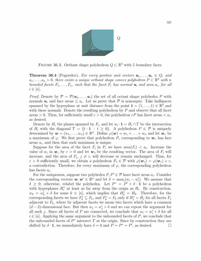
325

Q

Figure 36.3. Orthant shape polyhedron Q ⊂ R3 with 5 boundary faces.

Theorem 36.4 (Pogorelov). For every positive unit vectors u1, . . . ,un ∈ Q, anda1, . . . , an > 0, there exists a unique orthant shape convex polyhedron P ⊂ Rd with nbounded facets F1, . . . , Fn, such that the facet Fi has normal ui and area ai, for alli ∈ [n].

Proof. Denote by P = P(u1, . . . ,u i) the set of all octant shape polyhedra P withnormals u i and face areas ≤ ai. Let us prove that P is nonempty. Take halfspacesspanned by the hyperplane at unit distance from the point 1 = (1, . . . , 1) ∈ Rd andwith these normals. Denote the resulting polyhedron by P and observe that all facetareas > 0. Then, for sufficiently small c > 0, the polyhedron cP has facet areas < ai,as desired.

Denote by Hi the planes spanned by Fi, and let wi · 1 = Hi ∩ T be the intersectionof Hi with the diagonal T = t · 1 : t ≥ 0. A polyhedron P ∈ P is uniquelydetermined by w = (w1, . . . , wn) ∈ Rn. Define ϕ(w) = w1 + . . .+ wn and let w bea maximum of ϕ. We first prove that polyhedron P corresponding to w has faceareas ai, and then that such maximum is unique.

Suppose for the area of the facet Fi in P we have area(Fi) < ai. Increase thevalue of wi in w by ε > 0 and let w ⊳ be the resulting vector. The area of Fi willincrease, and the area of Fj , j 6= i, will decrease or remain unchanged. Thus, forε > 0 sufficiently small, we obtain a polyhedron P⊳ ∈ P with ϕ(w ⊳) = ϕ(w) + ε,a contradiction. Therefore, for every maximum of ϕ, the corresponding polyhedronhas facets ai.

For the uniqueness, suppose two polyhedra P, P ′ ∈ P have facet areas ai. Considerthe corresponding vectors w ,w ′ ∈ Rn and let δ = maxi(wi − w′

i). We assume thatδ ≥ 0; otherwise, relabel the polyhedra. Let P ∗ = P ′ + δ · 1 be a polyhedronwith hyperplanes H∗

i at least as far away from the origin as Hi. By construction,wk = w′

k + δ for some k ∈ [n], which implies that H∗k = Hk. Therefore, for the

corresponding facets we have F ∗k ⊆ Fk, and F ∗

k = Fk only if H∗j = Hj for all facets Fj

adjacent to Fk, where by adjacent facets we mean two facets which have a common(d− 2)-dimensional face. But then wj = w′

j + δ and we can repeat the argument forall such j. Since all facets of P are connected, we conclude that wi = w′

i + δ for alli ∈ [n]. Applying the same argument to the unbounded facets of P , we conclude thatthe unbounded facets of P ∗ intersect T at the origin. Since by construction they areshifted by δ · 1, we immediately have δ = 0 and P = P ∗ = P ′, as desired.

326

36.4. Alexandrov’s approach. Perhaps surprisingly, in R3 the Minkowski theoremcan be proved in two steps: first the uniqueness by the argument as in the Cauchytheorem (Theorem 26.1), and then by the topological argument as in the previoussection.

Theorem 36.5 (Alexandrov). Let P, P ′ ⊂ R3 be two convex polytopes with equal facenormals and such that neither face Fi in P fits inside the corresponding face F ′

i of P ′,nor vice versa. Then P and P ′ are congruent, i.e., equal up to a translation.

In particular, when the areas of the corresponding faces are equal, we obtain theuniqueness part of the Minkowski theorem without using the BrunnMinkowski in-equality. The existence part now can be done by a topological argument and is leftto the reader (Exercise 36.3).

36.5. Exercises.

Exercise 36.1. ♦ [1-] Make a translation of all hyperplanesHi and use equations area(Fi) =∂ vol(Pz )∂ zi

to obtain an alternative proof of Proposition 36.1.

Exercise 36.2. ♦ [1+] Use Alexandrov’s lemma (Theorem 22.4) to prove Alexandrov’sTheorem 36.5.

Exercise 36.3. ♦ [1+] Prove the Minkowski theorem in R3 using the Alexandrov theorem(Theorem 36.5) and the topological lemma (Theorem 41.8).

Exercise 36.4. ♦ [1+] Use Exercises 22.1 and 35.11 to obtain an alternative proof of theMinkowski theorem in R3, without the full power of the Alexandrov lemma (Theorem 22.4).

Exercise 36.5. ♦ a) [1-] In R3, prove the analogue of the Pogorelov theorem (Theo-rem 36.4) when perimeters of the faces are used in place of the areas.b) [1-] In R4, prove the analogue of the Pogorelov theorem (Theorem 36.4) when the surfacearea of the facets, which are 3-dimensional convex polytopes, are used in place of their 3-dimensional volumes.c) [1-] In R4, the same with mean curvatures.

Exercise 36.6. [∗] Find the perimeter analogue of the Minkowski theorem in R3?

Exercise 36.7. ♦ [1] Extend Pogorelov’s theorem to general convex cones in Rd.

Exercise 36.8. (Dihedral angles in simplices) a) [1-] Use Proposition 36.1 to prove thatevery facet of a simplex in Rd has an acute dihedral angle with some other facet.b) [1] Prove that every simplex in Rd has at least d acute dihedral angles.

Exercise 36.9. (Equihedral tetrahedra) ♦ [1+] Prove that every tetrahedron ∆ ⊂ R3 withequal face areas is equihedral (see Exercise 25.12).b) [1-] Prove that for all d ≥ 4, every simplex ∆ ⊂ Rd with equal areas of 2-dimensionalfaces is regular.

Exercise 36.10. (Shephard) A polytope P ⊂ Rd is called decomposable if P = P1 +P2 forsome polytopes which are not similar to P . Otherwise, P is called indecomposable.a) [1] Prove that except for a triangle, every convex polygon is decomposable.b) [1-] Prove that every simplicial polytope P ⊂ Rd is indecomposable.c) [1-] Prove that the truncated cube and the regular dodecahedron are decomposable.

327

d) [1+] Prove that except for a tetrahedron, every simple convex polytope in R3 is decom-posable.e) [1+] Find two combinatorially equivalent polytopes in R3, one of which is decomposableand the other is not.f) [2-] Suppose every two edges of a polytope P ⊂ R3 are connected by a chain of adjacenttriangles. Prove that P is indecomposable.g) [2-] Prove that every convex polytope P ⊂ R3 with n faces is the Minkowski sum of atmost n indecomposable polytopes.h) [2-] Generalize e), f) and g) to higher dimensions.

Exercise 36.11. (Wulff ) [1] Let P be a polytope defined by (k) in the proof of Theo-rem 36.5. Then P maximizes the sum z1 + . . . + zn among all polytopes P ′ with the samevolume and facet normals.

Exercise 36.12. (Lindelof ) Let P,P ′ ⊂ Rd be polytopes with the same face normalsu1, . . . ,un and facet areas ai = area(Fi) and a′i = area(F ′

i ), where i ∈ [n]. Denote by ziand z′i be as in Subsection 36.2.a) [1-] Define υ(P,P ′) = 1

d(z1a′1 + . . . + zna

′n). Observe that υ(P,P ) = dvol(P ). Check

that υ(P,P ′) is translation invariant.b) [1+] Fix P ′ and consider all P as above which satisfy υ(P,P ′) = dvol(P ′). Use Lagrangemultipliers to show that vol(P ) is maximized if and only if P is an expansion of P ′.c) [1+] Conclude that υ3(P,P ′) ≥ vol(P )vol(P ′)2 and the equality holds only if P is anexpansion of P ′.d) [1+] Let P ′ be a circumscribed polytope around a unit sphere. Observe that vol(P ′) =1d area(∂P ′). Prove that of all polytopes in Rd with given volume and facet normals, thecircumscribed polytope has the smallest surface area.e) [1-] Deduce from here the isoperimetric inequality.

Exercise 36.13. Let P,P ′ ⊂ Rd be convex polytopes as in the previous exercise.a) [1+] Define f(t) = P + tP ′. Prove that f ′(0) = υ(P,P ′).b) [1+] Use the Brunn–Minkowski inequality (see Proposition 7.7) to deduce part c) in theprevious exercise.c) [1] Conversely, deduce the Brunn–Minkowski inequality from part c) in the previousexercise.

Exercise 36.14. (Minkowski’s symmetry criterion) ♦ [1] Let P ⊂ Rd be a convex polytopesuch that for every facet F of P there exist a facet with the same area and opposite normal.Prove that P is centrally symmetric.

Exercise 36.15. (Zonotopes in Rd) ♦ a) [1] Suppose convex polytope P ⊂ Rd and all itsfaces are centrally symmetric. Prove that P is also centrally symmetric.b) [1+] Generalize Exercise 7.16 to prove that P is the Minkowski sum of intervals.

Exercise 36.16. Let P ⊂ Rd be a convex polytope such that translations of P tile thespace.a) [1] Prove that the opposite facets of P have equal areas.b) [1] Use the Minkowski theorem to prove that P is centrally symmetric.c) [1+] Extend this to show that all faces of P are centrally symmetric. Use the previousexercise to conclude that P is a zonotope.d) [1] In R3, show that P has at most 14 faces and this bound is tight.

328

e) [1+] Classify completely the combinatorics of all such P in R3.f) [1+] In Rd, show that P has at most 2d+1 − 2 facets.

Exercise 36.17. [∗] Suppose a convex polytope P ⊂ R3 can tile the whole space (notnecessarily periodically or even face-to-face). Prove that P has at most 106 vertices.

Exercise 36.18. a) [2-] Let P,P ′ ⊂ R3 be convex polytopes such that for every edge eof P there exists a parallel edge e′ of P ′ such that |e| ≤ |e′|. Suppose further, that for everyface F of P there exists a parallel face F ′ of P ′ such that a translation of F is containedin F ′. Prove that there exists a translation of P which is contained inside P ′.b) [1] Check that neither of the two conditions suffice by themselves.

Exercise 36.19. [2+] Find two convex polytopes P,Q ⊂ R3 with parallel and non-equalfaces which satisfy the following property: for every face F of P and the correspondingparallel face G of Q, there exists a unique translation which either fits F inside of G orfits G inside of F .82

36.6. Final remarks. Our proof of the Minkowski theorem is a reworking of Minkowski’soriginal proof [Min], parts of which were later clarified in [McM1]. The main idea of thisproof is implicitly based on Wulff’s theorem in crystallography (see [Grub, §8.4]). Letus mention that most standard proofs the Minkowski theorem are based on the Brunn–Minkowski inequality (see [BonF, Schn2]), to the extent that they can be shown essentiallyequivalent [Kla].83 Minkowski extended Theorem 36.2 to general surfaces (see [Pog4, Pog3]for further results and references). Let us mention also the algorithmic approach [GriH]and the important work on stability of solutions in the Minkowski theorem (see [Gro] andreferences therein).

The orthant shape variation given in Subsection 36.3 is due to Alexandrov, who provedit in [A2, §6.4] in the generality of all cones in R3 (cf. Exercise 36.7). It was extended tohigher dimensions and other functionals (see Exercise 36.5) by Pogorelov [Pog3, §7.6] (seealso [A2, §6.5] and [BarV]). The proof in Subsection 36.3 follows the original Pogorelov’sproof.

For the complete proof of the Alexandrov theorem (Theorem 36.5) see [A2, §6.2] (see

also [Lyu, §30] and [Mi3]). Let us mention that a series of Exercises 22.1, 35.11 and 36.4 out-

line a similar approach, which substitutes the tedious Alexandrov’s lemma (Theorem 22.4)

with an elegant argument in the Alexandrov’s local lemma (Exercise 22.1).

82The corresponding faces must lie on the same side of the polytopes; otherwise any tetrahedron Pand Q = −2P will work.

83To quote [Kla], they have “equiprimordial relationship.”

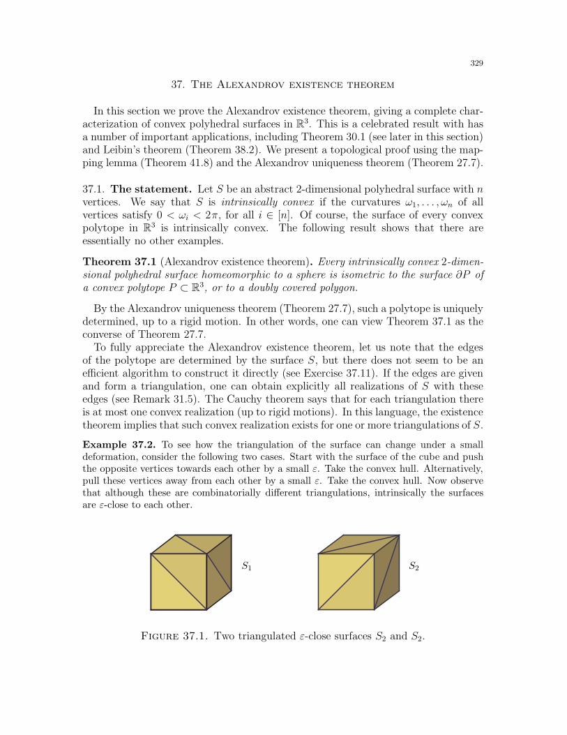
329

37. The Alexandrov existence theorem

In this section we prove the Alexandrov existence theorem, giving a complete char-acterization of convex polyhedral surfaces in R3. This is a celebrated result with hasa number of important applications, including Theorem 30.1 (see later in this section)and Leibin’s theorem (Theorem 38.2). We present a topological proof using the map-ping lemma (Theorem 41.8) and the Alexandrov uniqueness theorem (Theorem 27.7).

37.1. The statement. Let S be an abstract 2-dimensional polyhedral surface with nvertices. We say that S is intrinsically convex if the curvatures ω1, . . . , ωn of allvertices satisfy 0 < ωi < 2π, for all i ∈ [n]. Of course, the surface of every convexpolytope in R3 is intrinsically convex. The following result shows that there areessentially no other examples.

Theorem 37.1 (Alexandrov existence theorem). Every intrinsically convex 2-dimen-sional polyhedral surface homeomorphic to a sphere is isometric to the surface ∂P ofa convex polytope P ⊂ R3, or to a doubly covered polygon.

By the Alexandrov uniqueness theorem (Theorem 27.7), such a polytope is uniquelydetermined, up to a rigid motion. In other words, one can view Theorem 37.1 as theconverse of Theorem 27.7.

To fully appreciate the Alexandrov existence theorem, let us note that the edgesof the polytope are determined by the surface S, but there does not seem to be anefficient algorithm to construct it directly (see Exercise 37.11). If the edges are givenand form a triangulation, one can obtain explicitly all realizations of S with theseedges (see Remark 31.5). The Cauchy theorem says that for each triangulation thereis at most one convex realization (up to rigid motions). In this language, the existencetheorem implies that such convex realization exists for one or more triangulations of S.

Example 37.2. To see how the triangulation of the surface can change under a smalldeformation, consider the following two cases. Start with the surface of the cube and pushthe opposite vertices towards each other by a small ε. Take the convex hull. Alternatively,pull these vertices away from each other by a small ε. Take the convex hull. Now observethat although these are combinatorially different triangulations, intrinsically the surfacesare ε-close to each other.

S1 S2

Figure 37.1. Two triangulated ε-close surfaces S2 and S2.

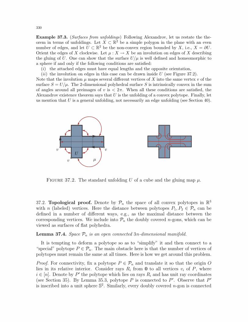
330

Example 37.3. (Surfaces from unfoldings) Following Alexandrov, let us restate the the-orem in terms of unfoldings. Let X ⊂ R2 be a simple polygon in the plane with an evennumber of edges, and let U ⊂ R2 be the non-convex region bounded by X, i.e., X = ∂U .Orient the edges of X clockwise. Let µ : X → X be an involution on edges of X describingthe gluing of U . One can show that the surface U/µ is well defined and homeomorphic toa sphere if and only if the following conditions are satisfied:

(i) the attached edges must have equal lengths and the opposite orientation,(ii) the involution on edges in this case can be drawn inside U (see Figure 37.2).

Note that the involution µ maps several different vertices of X into the same vertex v of thesurface S = U/µ. The 2-dimensional polyhedral surface S is intrinsically convex in the sumof angles around all preimages of v is < 2π. When all these conditions are satisfied, theAlexandrov existence theorem says that U is the unfolding of a convex polytope. Finally, letus mention that U is a general unfolding, not necessarily an edge unfolding (see Section 40).

U

µ

v v

v

Figure 37.2. The standard unfolding U of a cube and the gluing map µ.

37.2. Topological proof. Denote by Pn the space of all convex polytopes in R3

with n (labeled) vertices. Here the distance between polytopes P1, P2 ∈ Pn can bedefined in a number of different ways, e.g., as the maximal distance between thecorresponding vertices. We include into Pn the doubly covered n-gons, which can beviewed as surfaces of flat polyhedra.

Lemma 37.4. Space Pn is an open connected 3n-dimensional manifold.

It is tempting to deform a polytope so as to “simplify” it and then connect to a“special” polytope P ∈ Pn. The main obstacle here is that the number of vertices ofpolytopes must remain the same at all times. Here is how we get around this problem.

Proof. For connectivity, fix a polytope P ∈ Pn and translate it so that the origin Olies in its relative interior. Consider rays Ri from 0 to all vertices vi of P , wherei ∈ [n]. Denote by P ′ the polytope which lies on rays Ri and has unit ray coordinates(see Section 35). By Lemma 35.3, polytope P is connected to P ′. Observe that P ′

is inscribed into a unit sphere S2. Similarly, every doubly covered n-gon is connected

331

to a doubly covered n-gon inscribed into S2. Therefore, it suffices to show that allpolytopes in Pn inscribed into S2 are connected.

Let v′i ∈ S2 denote the vertices of P ′. By definition, P ′ = convv′1, . . . , v′n. Inthe other direction, for every u1, . . . , un ∈ S2 the polytope Q = convu1, . . . , un liesin Pn. Therefore, the space of polytopes Q ∈ Pn inscribed into S2 is homeomorphicto the space of distinct n-tuples of points in S2, and thus connected.

Now, take P ∈ Pn and perturb the vertices. When the perturbations are sufficientlysmall they give a convex polytope. The space of perturbations is 3n-dimensional,which implies that Pn is an open 3n-dimensional manifold.

Denote byMn the space of all 2-dimensional polyhedral surfaces homeomorphic toa sphere with n (labeled) vertices, defined as points with positive curvature. Again,the topology on Mn can be defined via the pairwise geodesic distance between thecorresponding vertices.

Lemma 37.5. Space Mn is an open connected (3n− 6)-dimensional manifold.

Proof. Take S ∈ Mn with vertices v1, . . . , vn. Fix a shortest path γij between viand vj , for all 1 ≤ i < j ≤ n. If there is more than one such path, choose either one.Since S is intrinsically convex, by Proposition 10.1 paths γij do not contain verticesin its relative interior. The geodesic triangle ∆ = γ12∪γ13∪γ23 subdivides S into tworegions. Vertex v4 lies in one of these regions and connected by γ14, γ24 and γ34 tothe vertices in its boundary. Vertex v5 lies in in one of the resulting four regions, etc.Denote by T the resulting geodesic triangulation of S. Observe that T has 3n − 6edges (see Corollary 25.2 or use induction in the construction).

By construction, every triangle in T is flat, i.e., has no vertices in its interior.Perturb the edge lengths of T . Since every vertex vi has, by definition, strictlypositive curvature, when the perturbations are sufficiently small they determine asurface S ′ ∈Mn. Thus,Mn is open and the space of such perturbations is (3n− 6)-dimensional.

To prove that Mn is connected, let us show that triangulation T can be realizedin R3 with the length function ℓij = |γij| (see Subsection 31.1). In other words,we claim that there exists a (possibly, self-intersecting) polyhedral surface S ⊂ R3

isometric to S, and such that S is triangulated into flat triangles according to T ,with the same edge lengths ℓij .

Use the construction of T . Suppose vertex vn is connected to a geodesic triangle[vivjvk]. The geodesic triangles A1 = [vnvivj], A2 = [vnvivk] and A3 = [vnvjvk] are flatand their angles at vn are together < 2π and satisfy the triangle inequality. Thus,there exists a tetrahedron in R3 with faces A1, A2 and A3. Change S into a surface S1

by substituting A1, A2 and A3 with a flat triangle [vivjvk]. Since the vertex curvaturesdo not increase, we conclude that S1 ∈ Mn−1.

84 Repeat the construction. At theend, we obtain a doubly covered triangle Sn−3 ∈ M3, which can be realized in R3.Going backwards, we obtain the desired realization S.

84Although γij in the surface S1 may no longer be the shortest paths, they are still geodesics anddefine a geodesic triangulation of S1.

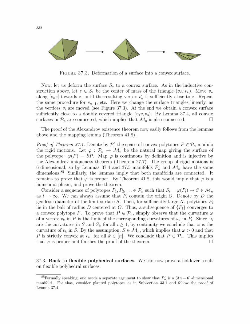
332

Figure 37.3. Deformation of a surface into a convex surface.

Now, let us deform the surface S to a convex surface. As in the inductive con-struction above, let z ∈ S1 be the center of mass of the triangle (vivivk). Move vnalong [vnz] towards z, until the resulting vertex v′n is sufficiently close to z. Repeatthe same procedure for vn−1, etc. Here we change the surface triangles linearly, asthe vertices vi are moved (see Figure 37.3). At the end we obtain a convex surfacesufficiently close to a doubly covered triangle (v1v2v3). By Lemma 37.4, all convexsurfaces in Pn are connected, which implies thatMn is also connected.

The proof of the Alexandrov existence theorem now easily follows from the lemmasabove and the mapping lemma (Theorem 41.8).

Proof of Theorem 37.1. Denote by P ′n the space of convex polytopes P ∈ Pn modulo

the rigid motions. Let ϕ : Pn → Mn be the natural map giving the surface ofthe polytope: ϕ(P ) = ∂P . Map ϕ is continuous by definition and is injective bythe Alexandrov uniqueness theorem (Theorem 27.7). The group of rigid motions is6-dimensional, so by Lemmas 37.4 and 37.5 manifolds P ′

n and Mn have the samedimensions.85 Similarly, the lemmas imply that both manifolds are connected. Itremains to prove that ϕ is proper. By Theorem 41.8, this would imply that ϕ is ahomeomorphism, and prove the theorem.

Consider a sequence of polytopes P1, P2, . . . ∈ Pn such that Si = ϕ(Pi)→ S ∈Mn

as i → ∞. We can always assume that Pi contain the origin O. Denote by D thegeodesic diameter of the limit surface S. Then, for sufficiently large N , polytopes Pilie in the ball of radius D centered at O. Thus, a subsequence of Pi converges toa convex polytope P . To prove that P ∈ Pn, simply observe that the curvature ωof a vertex vk in P is the limit of the corresponding curvatures of ωi in Pi. Since ωiare the curvatures in S and Si, for all i ≥ 1, by continuity we conclude that ω is thecurvature of vk in S. By the assumption, S ∈Mn, which implies that ω > 0 and thatP is strictly convex at vk, for all k ∈ [n]. We conclude that P ∈ Pn. This impliesthat ϕ is proper and finishes the proof of the theorem.

37.3. Back to flexible polyhedral surfaces. We can now prove a holdover resulton flexible polyhedral surfaces.

85Formally speaking, one needs a separate argument to show that P ′

n is a (3n − 6)-dimensionalmanifold. For that, consider planted polytopes as in Subsection 33.1 and follow the proof ofLemma 37.4.

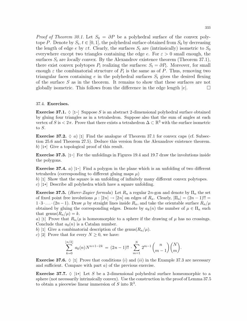
333

Proof of Theorem 30.1. Let S0 = ∂P be a polyhedral surface of the convex poly-tope P . Denote by St, t ∈ [0, 1], the polyhedral surface obtained from S0 by decreasingthe length of edge e by εt. Clearly, the surfaces St are (intrinsically) isometric to S0

everywhere except two triangles containing the edge e. For ε > 0 small enough, thesurfaces St are locally convex. By the Alexandrov existence theorem (Theorem 37.1),there exist convex polytopes Pt realizing the surfaces: St = ∂Pt. Moreover, for smallenough ε the combinatorial structure of Pt is the same as of P . Thus, removing twotriangular faces containing e in the polyhedral surfaces St gives the desired flexingof the surface S as in the theorem. It remains to show that these surfaces are notglobally isometric. This follows from the difference in the edge length |e|.

37.4. Exercises.

Exercise 37.1. ♦ [1-] Suppose S is an abstract 2-dimensional polyhedral surface obtainedby gluing four triangles as in a tetrahedron. Suppose also that the sum of angles at eachvertex of S is < 2π. Prove that there exists a tetrahedron ∆ ⊂ R3 with the surface isometricto S.

Exercise 37.2. ♦ a) [1] Find the analogue of Theorem 37.1 for convex caps (cf. Subsec-tion 25.6 and Theorem 27.5). Deduce this version from the Alexandrov existence theorem.b) [1+] Give a topological proof of this result.

Exercise 37.3. [1-] For the unfoldings in Figures 19.4 and 19.7 draw the involutions insidethe polygons.

Exercise 37.4. a) [1-] Find a polygon in the plane which is an unfolding of two differenttetrahedra (corresponding to different gluing maps µ)b) [1] Show that the square is an unfolding of infinitely many different convex polytopes.c) [1+] Describe all polyhedra which have a square unfolding.

Exercise 37.5. (Harer-Zagier formula) Let Rn a regular 2n-gon and denote by Πn the setof fixed point free involutions µ : [2n] → [2n] on edges of Rn. Clearly, |Πn| = (2n − 1)!! =1 · 3 · . . . · (2n− 1). Draw µ by straight lines inside Rn, and take the orientable surface Rn/µobtained by gluing the corresponding edges. Denote by ak(n) the number of µ ∈ Πn suchthat genus(Rn/µ) = k.a) [1] Prove that Rn/µ is homeomorphic to a sphere if the drawing of µ has no crossings.Conclude that a0(n) is a Catalan number.b) [1] Give a combinatorial description of the genus(Rn/µ).c) [2] Prove that for every N ≥ 0, we have:

⌊n/2⌋∑

k=0

ak(n)Nn+1−2k = (2n− 1)!! ·N∑

m=1

2m−1

(n

m− 1

)(N

m

).

Exercise 37.6. ♦ [1] Prove that conditions (i) and (ii) in the Example 37.3 are necessaryand sufficient. Compare with part a) of the previous exercise.

Exercise 37.7. ♦ [1+] Let S be a 2-dimensional polyhedral surface homeomorphic to asphere (not necessarily intrinsically convex). Use the construction in the proof of Lemma 37.5to obtain a piecewise linear immersion of S into R3.

334

Exercise 37.8. Start with unfolding the regular icosahedron given in Figure 19.4. Perturbthe edges by at most ε so that the corresponding edges under µ remain of the same length.b) [1-] Use the Alexandrov existence theorem to prove that for sufficiently small ε this isan unfolding of a convex polytope. Find an explicit bound on ε.b) [1] Use the algebraic approach in Section 31 to show that for sufficiently small ε this isan edge unfolding of a convex polytope combinatorially equivalent to the icosahedron.c) [1] Use the proof of the Alexandrov existence theorem to obtain part b). Explain theconnection to the proof of b).

Exercise 37.9. (Twisting the surfaces) Let S = ∂P be the surface of a convex polytopeP ⊂ R3, and let γ ⊂ S be a closed geodesic. Denote by S1 and S2 the surfaces on bothsides of γ. A surface S′ obtained by gluing S1 and S2 along the boundary is called a twistof S.a) [1-] Use the Alexandrov existence theorem to check that all surface twists are surfacesof convex polytopes.b) [1+] Start with a regular tetrahedron. Check that all polytopes obtained by a sequence oftwists must be equihedral tetrahedra (see Exercise 25.12). Prove or disprove: all equihedraltetrahedra with equal surface area can be obtained this way.c) [∗] Start with a square pyramid where all vertices have equal curvatures. Describe allpolytopes resulted by a sequence of twists.d) [∗] Same question for a regular octahedron.

Exercise 37.10. (Volkov’s stability theorem) ♦ [2+] Let S, S′ two intrinsically convex2-dimensional polyhedral surfaces homeomorphic to a sphere with geodesic diameter atmost 1. Suppose φ : S → S′ is a homeomorphism such that

|x, y|S − ε < |φ(x), φ(y)|S′ < |x, y|S + ε, for all x, y ∈ S .Denote by P,P ′ ⊂ R3 the corresponding convex polytopes. Prove that there exists a rigidmotion such that P and P ′ are “close to each other”:

|z, φ(z)| < C · ε1/24 , for all z ∈ ∂P (so that φ(z) ∈ ∂P ′),

and where C is a universal constant.

Exercise 37.11. [∗] Prove or disprove: computing edges in the polytope corresponding toa given intrinsically convex 2-dimensional polyhedral surface is NP-hard.

37.5. Final remarks. The Alexandrov existence theorem and its unbounded variations(cf. Subsection 27.3) was proved by Alexandrov in a series of papers. He presented twointerrelated proofs in [A1, A2], both based on elementary but delicate work with unfoldings.The proof in this section is largely new, although the use of the mapping lemma is motivatedby the proof in [A2].

A variational proof for the case of polyhedral caps (see Exercise 37.2) was given byVolkov in [Vol2], and was extended to general polytopes and general unbounded polyhe-dra in [VP1]. This proof was motivated by Pogorelov’s proof in Subsection 35.5. Mostrecently, a conceptual variational proof was found in [BobI], which also proved amenableto a computer implementation. This proof builds on top of Volkov’s proof and uses severaltechnical innovations, including an extension of the Alexandrov–Fenchel inequality, which isan advanced extension of the Brunn–Minkowski inequality and other geometric inequalities.An accessible exposition of the convex cap variation is given in [Izm].

335

Let us mention here an important Volkov’s stability theorem (Exercise 37.10), which he

proved for both bounded convex surfaces and for the convex caps [Vol3]. In a different di-

rection, the Burago–Zalgaller theorem is a non-convex analogue of the Alexandrov existence

theorem (see Exercise 39.13 and compare with Exercise 37.7).

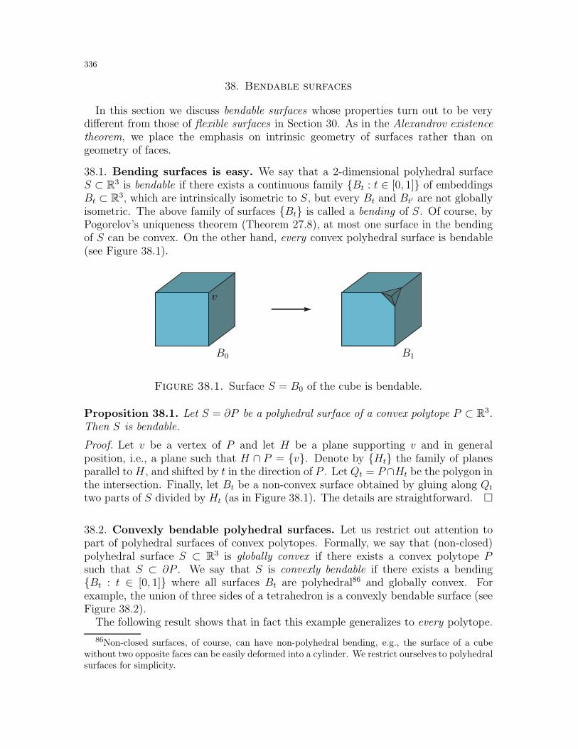
336

38. Bendable surfaces

In this section we discuss bendable surfaces whose properties turn out to be verydifferent from those of flexible surfaces in Section 30. As in the Alexandrov existencetheorem, we place the emphasis on intrinsic geometry of surfaces rather than ongeometry of faces.

38.1. Bending surfaces is easy. We say that a 2-dimensional polyhedral surfaceS ⊂ R3 is bendable if there exists a continuous family Bt : t ∈ [0, 1] of embeddingsBt ⊂ R3, which are intrinsically isometric to S, but every Bt and Bt′ are not globallyisometric. The above family of surfaces Bt is called a bending of S. Of course, byPogorelov’s uniqueness theorem (Theorem 27.8), at most one surface in the bendingof S can be convex. On the other hand, every convex polyhedral surface is bendable(see Figure 38.1).

B1B0

v

Figure 38.1. Surface S = B0 of the cube is bendable.

Proposition 38.1. Let S = ∂P be a polyhedral surface of a convex polytope P ⊂ R3.Then S is bendable.

Proof. Let v be a vertex of P and let H be a plane supporting v and in generalposition, i.e., a plane such that H ∩ P = v. Denote by Ht the family of planesparallel to H , and shifted by t in the direction of P . Let Qt = P∩Ht be the polygon inthe intersection. Finally, let Bt be a non-convex surface obtained by gluing along Qt

two parts of S divided by Ht (as in Figure 38.1). The details are straightforward.

38.2. Convexly bendable polyhedral surfaces. Let us restrict out attention topart of polyhedral surfaces of convex polytopes. Formally, we say that (non-closed)polyhedral surface S ⊂ R3 is globally convex if there exists a convex polytope Psuch that S ⊂ ∂P . We say that S is convexly bendable if there exists a bendingBt : t ∈ [0, 1] where all surfaces Bt are polyhedral86 and globally convex. Forexample, the union of three sides of a tetrahedron is a convexly bendable surface (seeFigure 38.2).

The following result shows that in fact this example generalizes to every polytope.

86Non-closed surfaces, of course, can have non-polyhedral bending, e.g., the surface of a cubewithout two opposite faces can be easily deformed into a cylinder. We restrict ourselves to polyhedralsurfaces for simplicity.

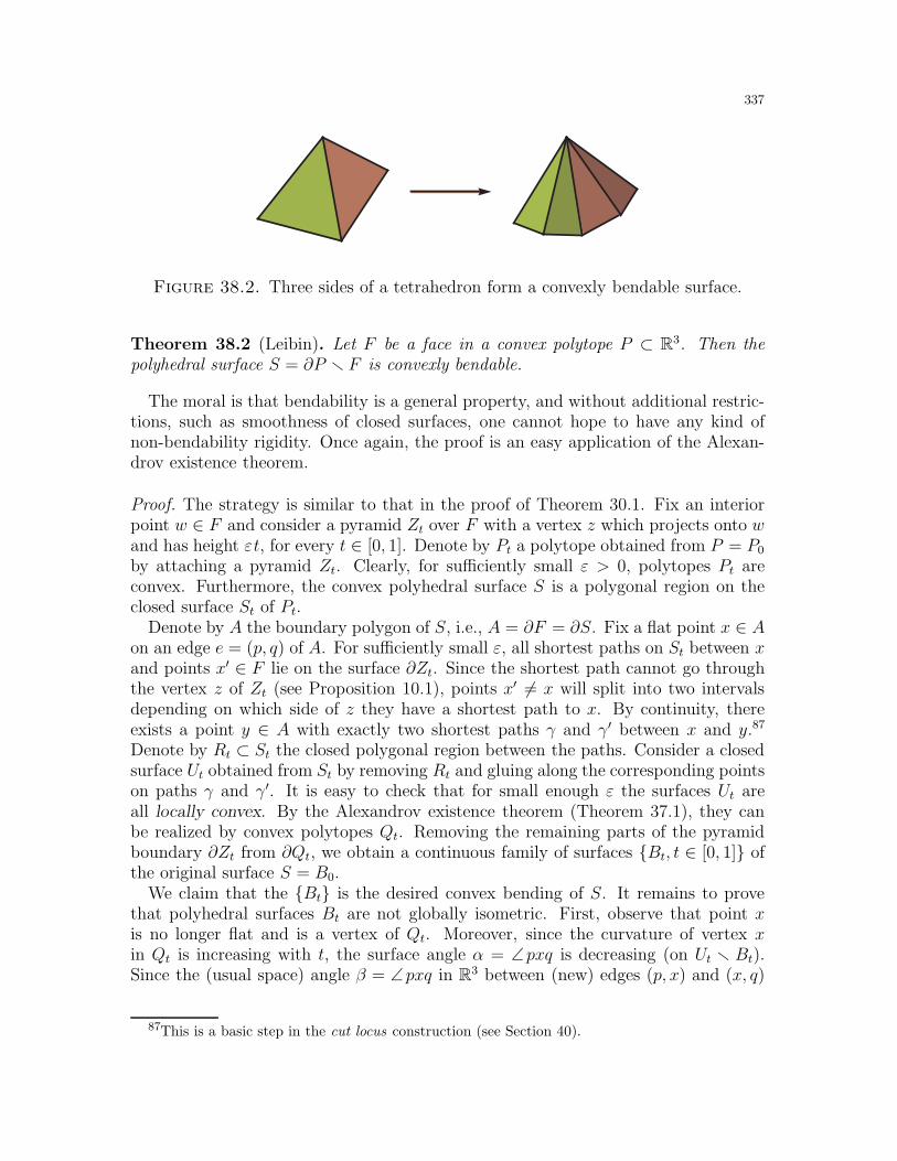
337

Figure 38.2. Three sides of a tetrahedron form a convexly bendable surface.

Theorem 38.2 (Leibin). Let F be a face in a convex polytope P ⊂ R3. Then thepolyhedral surface S = ∂P r F is convexly bendable.

The moral is that bendability is a general property, and without additional restric-tions, such as smoothness of closed surfaces, one cannot hope to have any kind ofnon-bendability rigidity. Once again, the proof is an easy application of the Alexan-drov existence theorem.

Proof. The strategy is similar to that in the proof of Theorem 30.1. Fix an interiorpoint w ∈ F and consider a pyramid Zt over F with a vertex z which projects onto wand has height εt, for every t ∈ [0, 1]. Denote by Pt a polytope obtained from P = P0

by attaching a pyramid Zt. Clearly, for sufficiently small ε > 0, polytopes Pt areconvex. Furthermore, the convex polyhedral surface S is a polygonal region on theclosed surface St of Pt.

Denote by A the boundary polygon of S, i.e., A = ∂F = ∂S. Fix a flat point x ∈ Aon an edge e = (p, q) of A. For sufficiently small ε, all shortest paths on St between xand points x′ ∈ F lie on the surface ∂Zt. Since the shortest path cannot go throughthe vertex z of Zt (see Proposition 10.1), points x′ 6= x will split into two intervalsdepending on which side of z they have a shortest path to x. By continuity, thereexists a point y ∈ A with exactly two shortest paths γ and γ′ between x and y.87

Denote by Rt ⊂ St the closed polygonal region between the paths. Consider a closedsurface Ut obtained from St by removing Rt and gluing along the corresponding pointson paths γ and γ′. It is easy to check that for small enough ε the surfaces Ut areall locally convex. By the Alexandrov existence theorem (Theorem 37.1), they canbe realized by convex polytopes Qt. Removing the remaining parts of the pyramidboundary ∂Zt from ∂Qt, we obtain a continuous family of surfaces Bt, t ∈ [0, 1] ofthe original surface S = B0.

We claim that the Bt is the desired convex bending of S. It remains to provethat polyhedral surfaces Bt are not globally isometric. First, observe that point xis no longer flat and is a vertex of Qt. Moreover, since the curvature of vertex xin Qt is increasing with t, the surface angle α = ∠pxq is decreasing (on Ut r Bt).Since the (usual space) angle β = ∠pxq in R3 between (new) edges (p, x) and (x, q)

87This is a basic step in the cut locus construction (see Section 40).

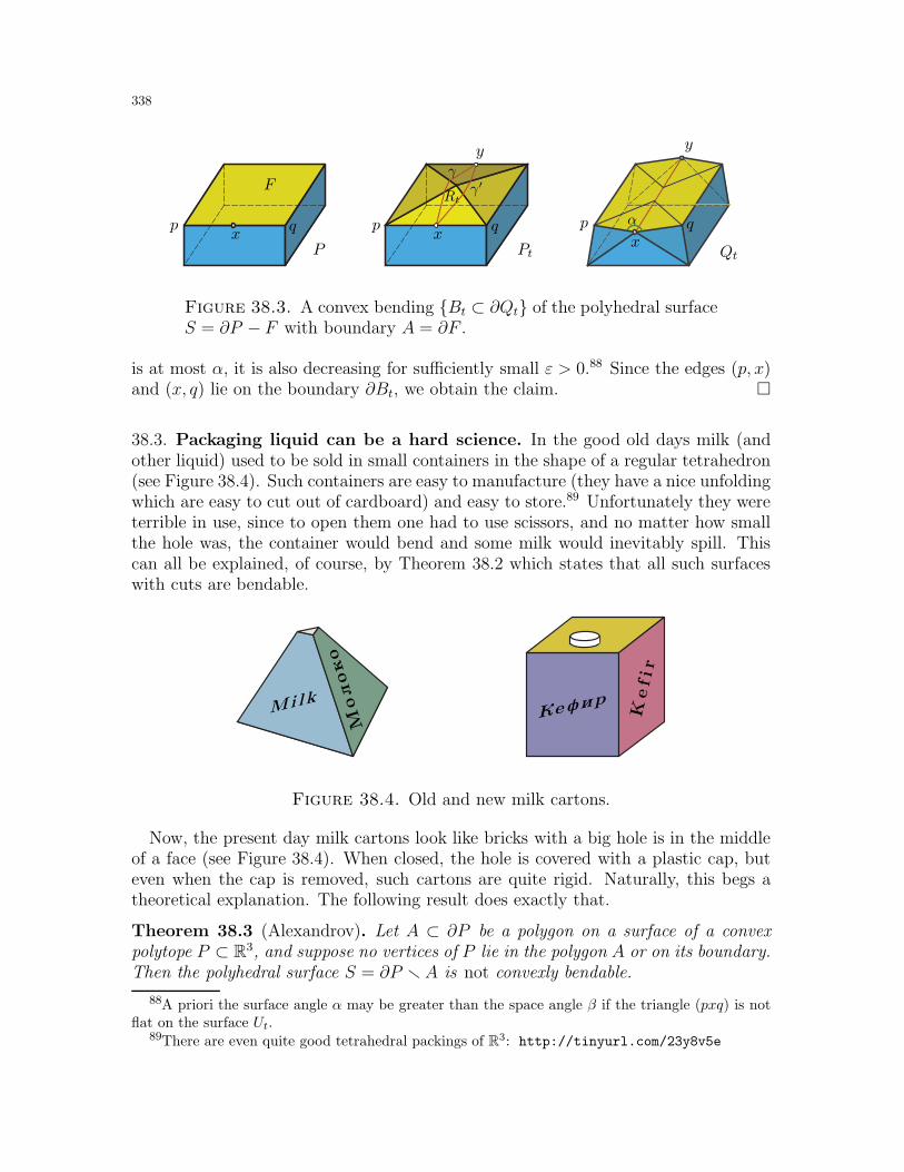
338

α

γγ′

ppp qqqxxx

yy

P QtPt

Rt

F

Figure 38.3. A convex bending Bt ⊂ ∂Qt of the polyhedral surfaceS = ∂P − F with boundary A = ∂F .

is at most α, it is also decreasing for sufficiently small ε > 0.88 Since the edges (p, x)and (x, q) lie on the boundary ∂Bt, we obtain the claim.

38.3. Packaging liquid can be a hard science. In the good old days milk (andother liquid) used to be sold in small containers in the shape of a regular tetrahedron(see Figure 38.4). Such containers are easy to manufacture (they have a nice unfoldingwhich are easy to cut out of cardboard) and easy to store.89 Unfortunately they wereterrible in use, since to open them one had to use scissors, and no matter how smallthe hole was, the container would bend and some milk would inevitably spill. Thiscan all be explained, of course, by Theorem 38.2 which states that all such surfaceswith cuts are bendable.

Kefir

Kefi r

Moloko

Milk

Figure 38.4. Old and new milk cartons.

Now, the present day milk cartons look like bricks with a big hole is in the middleof a face (see Figure 38.4). When closed, the hole is covered with a plastic cap, buteven when the cap is removed, such cartons are quite rigid. Naturally, this begs atheoretical explanation. The following result does exactly that.

Theorem 38.3 (Alexandrov). Let A ⊂ ∂P be a polygon on a surface of a convexpolytope P ⊂ R3, and suppose no vertices of P lie in the polygon A or on its boundary.Then the polyhedral surface S = ∂P r A is not convexly bendable.

88A priori the surface angle α may be greater than the space angle β if the triangle (pxq) is notflat on the surface Ut.

89There are even quite good tetrahedral packings of R3: http://tinyurl.com/23y8v5e

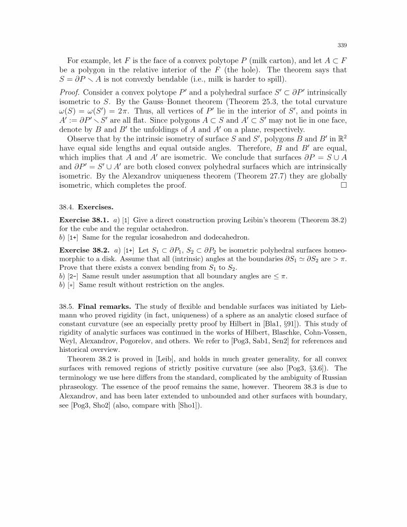
339

For example, let F is the face of a convex polytope P (milk carton), and let A ⊂ Fbe a polygon in the relative interior of the F (the hole). The theorem says thatS = ∂P rA is not convexly bendable (i.e., milk is harder to spill).

Proof. Consider a convex polytope P ′ and a polyhedral surface S ′ ⊂ ∂P ′ intrinsicallyisometric to S. By the Gauss–Bonnet theorem (Theorem 25.3, the total curvatureω(S) = ω(S ′) = 2π. Thus, all vertices of P ′ lie in the interior of S ′, and points inA′ := ∂P ′rS ′ are all flat. Since polygons A ⊂ S and A′ ⊂ S ′ may not lie in one face,denote by B and B′ the unfoldings of A and A′ on a plane, respectively.

Observe that by the intrinsic isometry of surface S and S ′, polygons B and B′ in R2

have equal side lengths and equal outside angles. Therefore, B and B′ are equal,which implies that A and A′ are isometric. We conclude that surfaces ∂P = S ∪ Aand ∂P ′ = S ′ ∪A′ are both closed convex polyhedral surfaces which are intrinsicallyisometric. By the Alexandrov uniqueness theorem (Theorem 27.7) they are globallyisometric, which completes the proof.

38.4. Exercises.

Exercise 38.1. a) [1] Give a direct construction proving Leibin’s theorem (Theorem 38.2)for the cube and the regular octahedron.b) [1+] Same for the regular icosahedron and dodecahedron.

Exercise 38.2. a) [1+] Let S1 ⊂ ∂P1, S2 ⊂ ∂P2 be isometric polyhedral surfaces homeo-morphic to a disk. Assume that all (intrinsic) angles at the boundaries ∂S1 ≃ ∂S2 are > π.Prove that there exists a convex bending from S1 to S2.b) [2-] Same result under assumption that all boundary angles are ≤ π.b) [∗] Same result without restriction on the angles.

38.5. Final remarks. The study of flexible and bendable surfaces was initiated by Lieb-mann who proved rigidity (in fact, uniqueness) of a sphere as an analytic closed surface ofconstant curvature (see an especially pretty proof by Hilbert in [Bla1, §91]). This study ofrigidity of analytic surfaces was continued in the works of Hilbert, Blaschke, Cohn-Vossen,Weyl, Alexandrov, Pogorelov, and others. We refer to [Pog3, Sab1, Sen2] for references andhistorical overview.

Theorem 38.2 is proved in [Leib], and holds in much greater generality, for all convex

surfaces with removed regions of strictly positive curvature (see also [Pog3, §3.6]). The

terminology we use here differs from the standard, complicated by the ambiguity of Russian

phraseology. The essence of the proof remains the same, however. Theorem 38.3 is due to

Alexandrov, and has been later extended to unbounded and other surfaces with boundary,

see [Pog3, Sho2] (also, compare with [Sho1]).

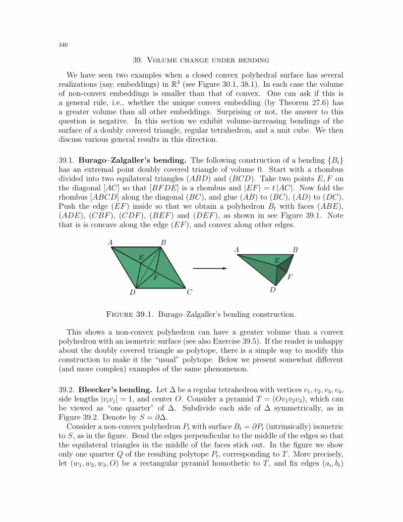
340

39. Volume change under bending

We have seen two examples when a closed convex polyhedral surface has severalrealizations (say, embeddings) in R3 (see Figure 30.1, 38.1). In each case the volumeof non-convex embeddings is smaller than that of convex. One can ask if this isa general rule, i.e., whether the unique convex embedding (by Theorem 27.6) hasa greater volume than all other embeddings. Surprising or not, the answer to thisquestion is negative. In this section we exhibit volume-increasing bendings of thesurface of a doubly covered triangle, regular tetrahedron, and a unit cube. We thendiscuss various general results in this direction.

39.1. Burago–Zalgaller’s bending. The following construction of a bending Bthas an extremal point doubly covered triangle of volume 0. Start with a rhombusdivided into two equilateral triangles (ABD) and (BCD). Take two points E,F onthe diagonal [AC] so that [BFDE] is a rhombus and |EF | = t |AC|. Now fold therhombus [ABCD] along the diagonal (BC), and glue (AB) to (BC), (AD) to (DC).Push the edge (EF ) inside so that we obtain a polyhedron Bt with faces (ABE),(ADE), (CBF ), (CDF ), (BEF ) and (DEF ), as shown in see Figure 39.1. Notethat is is concave along the edge (EF ), and convex along other edges.

AA

BB

C DD

E E

F F

Figure 39.1. Burago–Zalgaller’s bending construction.

This shows a non-convex polyhedron can have a greater volume than a convexpolyhedron with an isometric surface (see also Exercise 39.5). If the reader is unhappyabout the doubly covered triangle as polytope, there is a simple way to modify thisconstruction to make it the “usual” polytope. Below we present somewhat different(and more complex) examples of the same phenomenon.

39.2. Bleecker’s bending. Let ∆ be a regular tetrahedron with vertices v1, v2, v3, v4,side lengths |vivj| = 1, and center O. Consider a pyramid T = (Ov1v2v3), which canbe viewed as “one quarter” of ∆. Subdivide each side of ∆ symmetrically, as inFigure 39.2. Denote by S = ∂∆.

Consider a non-convex polyhedron Pt with surface Bt = ∂Pt (intrinsically) isometricto S, as in the figure. Bend the edges perpendicular to the middle of the edges so thatthe equilateral triangles in the middle of the faces stick out. In the figure we showonly one quarter Q of the resulting polytope Pt, corresponding to T . More precisely,let (w1, w2, w3, O) be a rectangular pyramid homothetic to T , and fix edges (ai, bi)

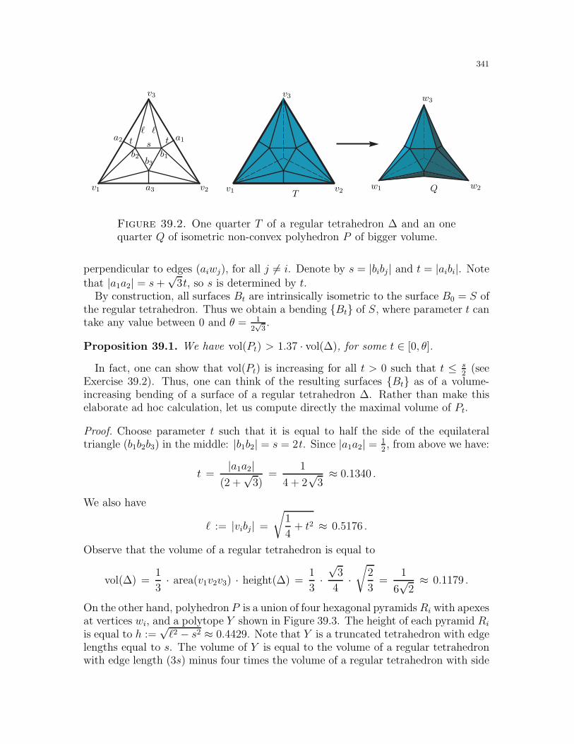
341

ℓℓ

s tt

v1v1 v2v2

v3v3

a1a2

a3

b1b2b3

TQw1 w2

w3

Figure 39.2. One quarter T of a regular tetrahedron ∆ and an onequarter Q of isometric non-convex polyhedron P of bigger volume.

perpendicular to edges (aiwj), for all j 6= i. Denote by s = |bibj | and t = |aibi|. Note

that |a1a2| = s+√

3t, so s is determined by t.By construction, all surfaces Bt are intrinsically isometric to the surface B0 = S of

the regular tetrahedron. Thus we obtain a bending Bt of S, where parameter t cantake any value between 0 and θ = 1

2√

3.

Proposition 39.1. We have vol(Pt) > 1.37 · vol(∆), for some t ∈ [0, θ].

In fact, one can show that vol(Pt) is increasing for all t > 0 such that t ≤ s2

(seeExercise 39.2). Thus, one can think of the resulting surfaces Bt as of a volume-increasing bending of a surface of a regular tetrahedron ∆. Rather than make thiselaborate ad hoc calculation, let us compute directly the maximal volume of Pt.

Proof. Choose parameter t such that it is equal to half the side of the equilateraltriangle (b1b2b3) in the middle: |b1b2| = s = 2t. Since |a1a2| = 1

2, from above we have:

t =|a1a2|

(2 +√

3)=

1

4 + 2√

3≈ 0.1340 .

We also have

ℓ := |vibj | =

√1

4+ t2 ≈ 0.5176 .

Observe that the volume of a regular tetrahedron is equal to

vol(∆) =1

3· area(v1v2v3) · height(∆) =

1

3·√

3

4·√

2

3=

1

6√

2≈ 0.1179 .

On the other hand, polyhedron P is a union of four hexagonal pyramids Ri with apexesat vertices wi, and a polytope Y shown in Figure 39.3. The height of each pyramid Ri

is equal to h :=√ℓ2 − s2 ≈ 0.4429. Note that Y is a truncated tetrahedron with edge

lengths equal to s. The volume of Y is equal to the volume of a regular tetrahedronwith edge length (3s) minus four times the volume of a regular tetrahedron with side

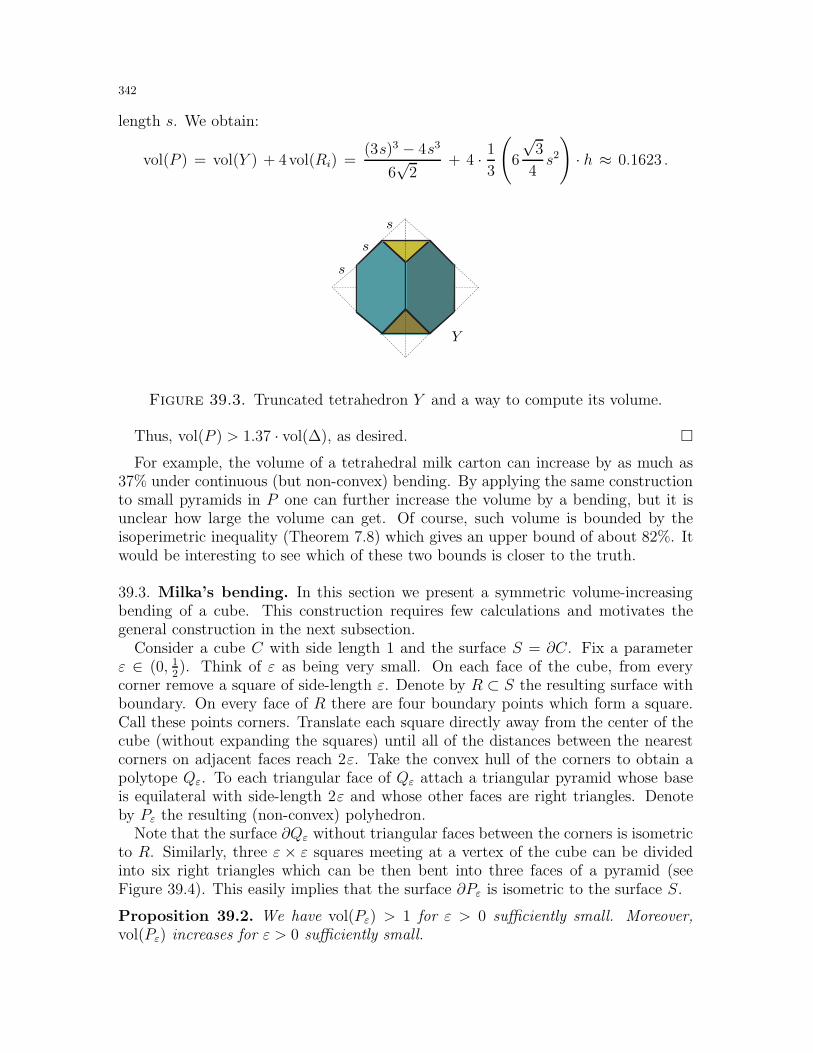
342

length s. We obtain:

vol(P ) = vol(Y ) + 4vol(Ri) =(3s)3 − 4s3

6√

2+ 4 · 1

3

(6

√3

4s2

)· h ≈ 0.1623 .

Y

s

s

s

Figure 39.3. Truncated tetrahedron Y and a way to compute its volume.

Thus, vol(P ) > 1.37 · vol(∆), as desired.

For example, the volume of a tetrahedral milk carton can increase by as much as37% under continuous (but non-convex) bending. By applying the same constructionto small pyramids in P one can further increase the volume by a bending, but it isunclear how large the volume can get. Of course, such volume is bounded by theisoperimetric inequality (Theorem 7.8) which gives an upper bound of about 82%. Itwould be interesting to see which of these two bounds is closer to the truth.

39.3. Milka’s bending. In this section we present a symmetric volume-increasingbending of a cube. This construction requires few calculations and motivates thegeneral construction in the next subsection.

Consider a cube C with side length 1 and the surface S = ∂C. Fix a parameterε ∈ (0, 1

2). Think of ε as being very small. On each face of the cube, from every

corner remove a square of side-length ε. Denote by R ⊂ S the resulting surface withboundary. On every face of R there are four boundary points which form a square.Call these points corners. Translate each square directly away from the center of thecube (without expanding the squares) until all of the distances between the nearestcorners on adjacent faces reach 2ε. Take the convex hull of the corners to obtain apolytope Qε. To each triangular face of Qε attach a triangular pyramid whose baseis equilateral with side-length 2ε and whose other faces are right triangles. Denoteby Pε the resulting (non-convex) polyhedron.

Note that the surface ∂Qε without triangular faces between the corners is isometricto R. Similarly, three ε × ε squares meeting at a vertex of the cube can be dividedinto six right triangles which can be then bent into three faces of a pyramid (seeFigure 39.4). This easily implies that the surface ∂Pε is isometric to the surface S.

Proposition 39.2. We have vol(Pε) > 1 for ε > 0 sufficiently small. Moreover,vol(Pε) increases for ε > 0 sufficiently small.

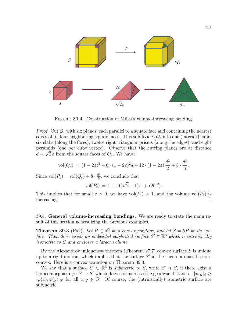
343

ϕ

C Qε

ε

ε

√2ε

2ε

2ε

Figure 39.4. Construction of Milka’s volume-increasing bending.

Proof. CutQε with six planes, each parallel to a square face and containing the nearestedges of its four neighboring square faces. This subdivides Qε into one (interior) cube,six slabs (along the faces), twelve right triangular prisms (along the edges), and eightpyramids (one per cube vertex). Observe that the cutting planes are at distanced =√

2 ε from the square faces of Qε. We have:

vol(Qε) = (1− 2ε)3 + 6 · (1− 2ε)2d+ 12 · (1− 2ε)d2

2+ 8 · d

3

6.

Since vol(Pε) = vol(Qε) + 8 · d36, we conclude that

vol(Pε) = 1 + 6(√

2− 1) ε + O(ε2),

This implies that for small ε > 0, we have vol(Pε) > 1, and the volume vol(Pε) isincreasing.

39.4. General volume-increasing bendings. We are ready to state the main re-sult of this section generalizing the previous examples.

Theorem 39.3 (Pak). Let P ⊂ R3 be a convex polytope, and let S = ∂P be its sur-face. Then there exists an embedded polyhedral surface S ′ ⊂ R3 which is intrinsicallyisometric to S and encloses a larger volume.

By the Alexandrov uniqueness theorem (Theorem 27.7) convex surface S is uniqueup to a rigid motion, which implies that the surface S ′ in the theorem must be non-convex. Here is a convex variation on Theorem 39.3.

We say that a surface S ′ ⊂ R3 is submetric to S, write S ′ 4 S, if there exist ahomeomorphism ϕ : S → S ′ which does not increase the geodesic distances: |x, y|S ≥|ϕ(x), ϕ(y)|S′ for all x, y ∈ S. Of course, the (intrinsically) isometric surface aresubmetric.

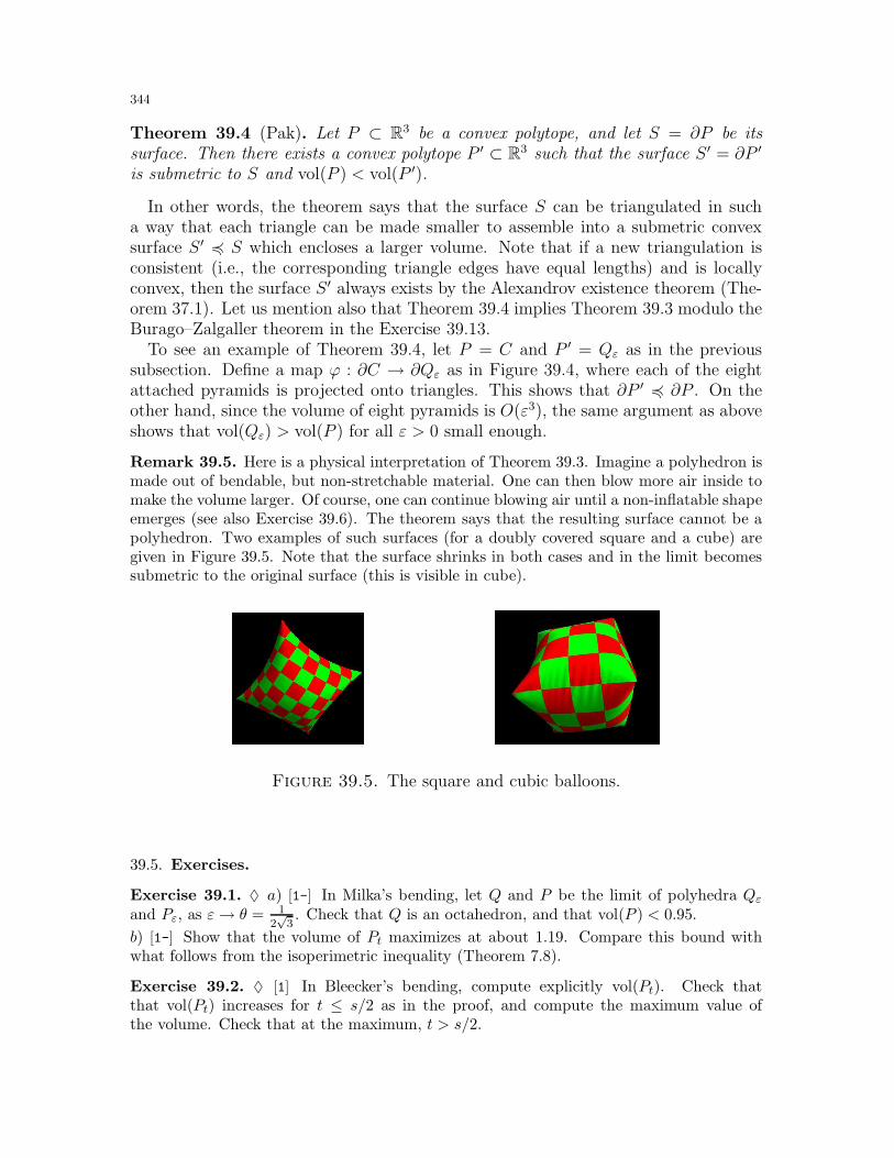
344

Theorem 39.4 (Pak). Let P ⊂ R3 be a convex polytope, and let S = ∂P be itssurface. Then there exists a convex polytope P ′ ⊂ R3 such that the surface S ′ = ∂P ′

is submetric to S and vol(P ) < vol(P ′).

In other words, the theorem says that the surface S can be triangulated in sucha way that each triangle can be made smaller to assemble into a submetric convexsurface S ′ 4 S which encloses a larger volume. Note that if a new triangulation isconsistent (i.e., the corresponding triangle edges have equal lengths) and is locallyconvex, then the surface S ′ always exists by the Alexandrov existence theorem (The-orem 37.1). Let us mention also that Theorem 39.4 implies Theorem 39.3 modulo theBurago–Zalgaller theorem in the Exercise 39.13.

To see an example of Theorem 39.4, let P = C and P ′ = Qε as in the previoussubsection. Define a map ϕ : ∂C → ∂Qε as in Figure 39.4, where each of the eightattached pyramids is projected onto triangles. This shows that ∂P ′ 4 ∂P . On theother hand, since the volume of eight pyramids is O(ε3), the same argument as aboveshows that vol(Qε) > vol(P ) for all ε > 0 small enough.

Remark 39.5. Here is a physical interpretation of Theorem 39.3. Imagine a polyhedron ismade out of bendable, but non-stretchable material. One can then blow more air inside tomake the volume larger. Of course, one can continue blowing air until a non-inflatable shapeemerges (see also Exercise 39.6). The theorem says that the resulting surface cannot be apolyhedron. Two examples of such surfaces (for a doubly covered square and a cube) aregiven in Figure 39.5. Note that the surface shrinks in both cases and in the limit becomessubmetric to the original surface (this is visible in cube).

Figure 39.5. The square and cubic balloons.

39.5. Exercises.

Exercise 39.1. ♦ a) [1-] In Milka’s bending, let Q and P be the limit of polyhedra Qεand Pε, as ε→ θ = 1

2√

3. Check that Q is an octahedron, and that vol(P ) < 0.95.

b) [1-] Show that the volume of Pt maximizes at about 1.19. Compare this bound withwhat follows from the isoperimetric inequality (Theorem 7.8).

Exercise 39.2. ♦ [1] In Bleecker’s bending, compute explicitly vol(Pt). Check thatthat vol(Pt) increases for t ≤ s/2 as in the proof, and compute the maximum value ofthe volume. Check that at the maximum, t > s/2.

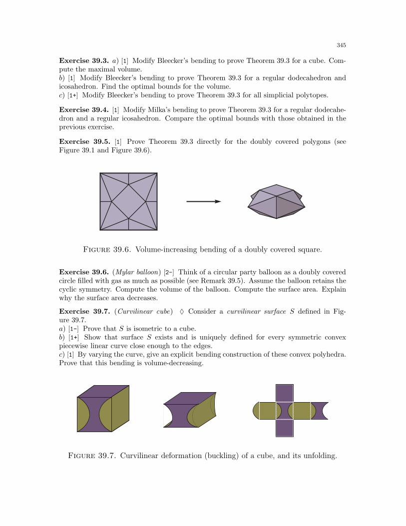
345

Exercise 39.3. a) [1] Modify Bleecker’s bending to prove Theorem 39.3 for a cube. Com-pute the maximal volume.b) [1] Modify Bleecker’s bending to prove Theorem 39.3 for a regular dodecahedron andicosahedron. Find the optimal bounds for the volume.c) [1+] Modify Bleecker’s bending to prove Theorem 39.3 for all simplicial polytopes.

Exercise 39.4. [1] Modify Milka’s bending to prove Theorem 39.3 for a regular dodecahe-dron and a regular icosahedron. Compare the optimal bounds with those obtained in theprevious exercise.

Exercise 39.5. [1] Prove Theorem 39.3 directly for the doubly covered polygons (seeFigure 39.1 and Figure 39.6).

Figure 39.6. Volume-increasing bending of a doubly covered square.

Exercise 39.6. (Mylar balloon) [2-] Think of a circular party balloon as a doubly coveredcircle filled with gas as much as possible (see Remark 39.5). Assume the balloon retains thecyclic symmetry. Compute the volume of the balloon. Compute the surface area. Explainwhy the surface area decreases.

Exercise 39.7. (Curvilinear cube) ♦ Consider a curvilinear surface S defined in Fig-ure 39.7.a) [1-] Prove that S is isometric to a cube.b) [1+] Show that surface S exists and is uniquely defined for every symmetric convexpiecewise linear curve close enough to the edges.c) [1] By varying the curve, give an explicit bending construction of these convex polyhedra.Prove that this bending is volume-decreasing.

Figure 39.7. Curvilinear deformation (buckling) of a cube, and its unfolding.

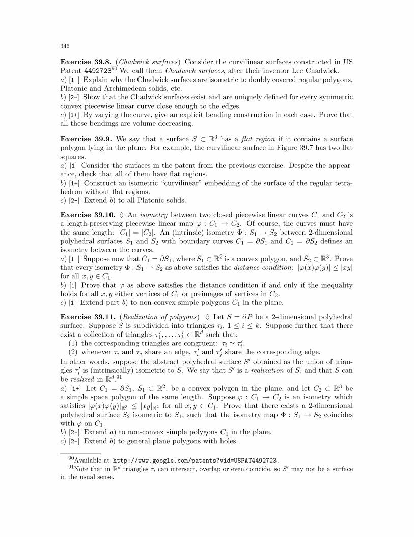
346

Exercise 39.8. (Chadwick surfaces) Consider the curvilinear surfaces constructed in USPatent 449272390 We call them Chadwick surfaces, after their inventor Lee Chadwick.a) [1-] Explain why the Chadwick surfaces are isometric to doubly covered regular polygons,Platonic and Archimedean solids, etc.b) [2-] Show that the Chadwick surfaces exist and are uniquely defined for every symmetricconvex piecewise linear curve close enough to the edges.c) [1+] By varying the curve, give an explicit bending construction in each case. Prove thatall these bendings are volume-decreasing.

Exercise 39.9. We say that a surface S ⊂ R3 has a flat region if it contains a surfacepolygon lying in the plane. For example, the curvilinear surface in Figure 39.7 has two flatsquares.a) [1] Consider the surfaces in the patent from the previous exercise. Despite the appear-ance, check that all of them have flat regions.b) [1+] Construct an isometric “curvilinear” embedding of the surface of the regular tetra-hedron without flat regions.c) [2-] Extend b) to all Platonic solids.

Exercise 39.10. ♦ An isometry between two closed piecewise linear curves C1 and C2 isa length-preserving piecewise linear map ϕ : C1 → C2. Of course, the curves must havethe same length: |C1| = |C2|. An (intrinsic) isometry Φ : S1 → S2 between 2-dimensionalpolyhedral surfaces S1 and S2 with boundary curves C1 = ∂S1 and C2 = ∂S2 defines anisometry between the curves.a) [1-] Suppose now that C1 = ∂S1, where S1 ⊂ R2 is a convex polygon, and S2 ⊂ R3. Provethat every isometry Φ : S1 → S2 as above satisfies the distance condition: |ϕ(x)ϕ(y)| ≤ |xy|for all x, y ∈ C1.b) [1] Prove that ϕ as above satisfies the distance condition if and only if the inequalityholds for all x, y either vertices of C1 or preimages of vertices in C2.c) [1] Extend part b) to non-convex simple polygons C1 in the plane.

Exercise 39.11. (Realization of polygons) ♦ Let S = ∂P be a 2-dimensional polyhedralsurface. Suppose S is subdivided into triangles τi, 1 ≤ i ≤ k. Suppose further that thereexist a collection of triangles τ ′1, . . . , τ

′k ⊂ Rd such that:

(1) the corresponding triangles are congruent: τi ≃ τ ′i ,(2) whenever τi and τj share an edge, τ ′i and τ ′j share the corresponding edge.

In other words, suppose the abstract polyhedral surface S′ obtained as the union of trian-gles τ ′i is (intrinsically) isometric to S. We say that S′ is a realization of S, and that S canbe realized in Rd.91

a) [1+] Let C1 = ∂S1, S1 ⊂ R2, be a convex polygon in the plane, and let C2 ⊂ R3 bea simple space polygon of the same length. Suppose ϕ : C1 → C2 is an isometry whichsatisfies |ϕ(x)ϕ(y)|R3 ≤ |xy|R2 for all x, y ∈ C1. Prove that there exists a 2-dimensionalpolyhedral surface S2 isometric to S1, such that the isometry map Φ : S1 → S2 coincideswith ϕ on C1.b) [2-] Extend a) to non-convex simple polygons C1 in the plane.c) [2-] Extend b) to general plane polygons with holes.

90Available at http://www.google.com/patents?vid=USPAT4492723.91Note that in Rd triangles τi can intersect, overlap or even coincide, so S′ may not be a surface

in the usual sense.

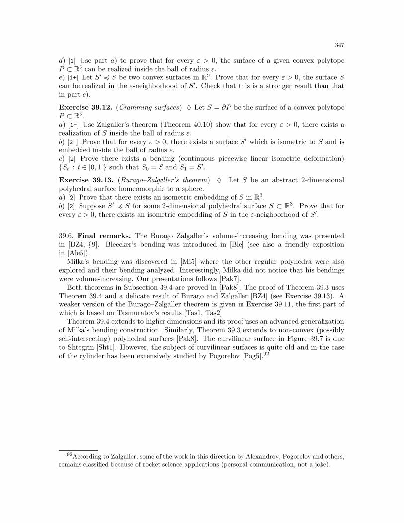
347

d) [1] Use part a) to prove that for every ε > 0, the surface of a given convex polytopeP ⊂ R3 can be realized inside the ball of radius ε.e) [1+] Let S′ 4 S be two convex surfaces in R3. Prove that for every ε > 0, the surface Scan be realized in the ε-neighborhood of S′. Check that this is a stronger result than thatin part c).

Exercise 39.12. (Cramming surfaces) ♦ Let S = ∂P be the surface of a convex polytopeP ⊂ R3.a) [1-] Use Zalgaller’s theorem (Theorem 40.10) show that for every ε > 0, there exists arealization of S inside the ball of radius ε.b) [2-] Prove that for every ε > 0, there exists a surface S′ which is isometric to S and isembedded inside the ball of radius ε.c) [2] Prove there exists a bending (continuous piecewise linear isometric deformation)St : t ∈ [0, 1] such that S0 = S and S1 = S′.

Exercise 39.13. (Burago–Zalgaller’s theorem) ♦ Let S be an abstract 2-dimensionalpolyhedral surface homeomorphic to a sphere.a) [2] Prove that there exists an isometric embedding of S in R3.b) [2] Suppose S′ 4 S for some 2-dimensional polyhedral surface S ⊂ R3. Prove that forevery ε > 0, there exists an isometric embedding of S in the ε-neighborhood of S′.

39.6. Final remarks. The Burago–Zalgaller’s volume-increasing bending was presentedin [BZ4, §9]. Bleecker’s bending was introduced in [Ble] (see also a friendly expositionin [Ale5]).

Milka’s bending was discovered in [Mi5] where the other regular polyhedra were alsoexplored and their bending analyzed. Interestingly, Milka did not notice that his bendingswere volume-increasing. Our presentations follows [Pak7].

Both theorems in Subsection 39.4 are proved in [Pak8]. The proof of Theorem 39.3 usesTheorem 39.4 and a delicate result of Burago and Zalgaller [BZ4] (see Exercise 39.13). Aweaker version of the Burago–Zalgaller theorem is given in Exercise 39.11, the first part ofwhich is based on Tasmuratov’s results [Tas1, Tas2]

Theorem 39.4 extends to higher dimensions and its proof uses an advanced generalizationof Milka’s bending construction. Similarly, Theorem 39.3 extends to non-convex (possiblyself-intersecting) polyhedral surfaces [Pak8]. The curvilinear surface in Figure 39.7 is dueto Shtogrin [Sht1]. However, the subject of curvilinear surfaces is quite old and in the caseof the cylinder has been extensively studied by Pogorelov [Pog5].92

92According to Zalgaller, some of the work in this direction by Alexandrov, Pogorelov and others,remains classified because of rocket science applications (personal communication, not a joke).

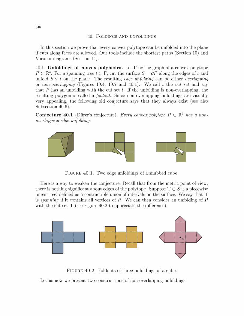
348

40. Foldings and unfoldings

In this section we prove that every convex polytope can be unfolded into the planeif cuts along faces are allowed. Our tools include the shortest paths (Section 10) andVoronoi diagrams (Section 14).

40.1. Unfoldings of convex polyhedra. Let Γ be the graph of a convex polytopeP ⊂ R3. For a spanning tree t ⊂ Γ, cut the surface S = ∂P along the edges of t andunfold S r t on the plane. The resulting edge unfolding can be either overlappingor non-overlapping (Figures 19.4, 19.7 and 40.1). We call t the cut set and saythat P has an unfolding with the cut set t. If the unfolding is non-overlapping, theresulting polygon is called a foldout. Since non-overlapping unfoldings are visuallyvery appealing, the following old conjecture says that they always exist (see alsoSubsection 40.6).

Conjecture 40.1 (Durer’s conjecture). Every convex polytope P ⊂ R3 has a non-overlapping edge unfolding.

Figure 40.1. Two edge unfoldings of a snubbed cube.

Here is a way to weaken the conjecture. Recall that from the metric point of view,there is nothing significant about edges of the polytope. Suppose T ⊂ S is a piecewiselinear tree, defined as a contractible union of intervals on the surface. We say that Tis spanning if it contains all vertices of P . We can then consider an unfolding of Pwith the cut set T (see Figure 40.2 to appreciate the difference).

w

Figure 40.2. Foldouts of three unfoldings of a cube.

Let us now we present two constructions of non-overlapping unfoldings.

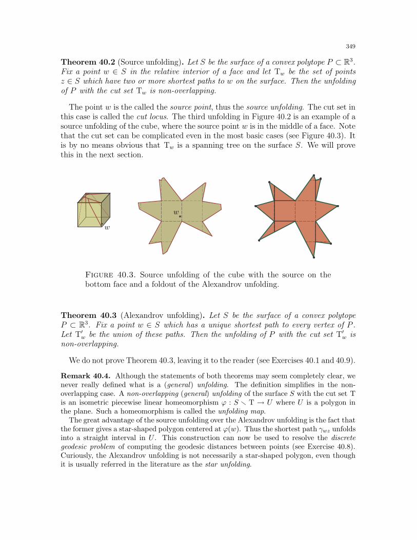
349

Theorem 40.2 (Source unfolding). Let S be the surface of a convex polytope P ⊂ R3.Fix a point w ∈ S in the relative interior of a face and let Tw be the set of pointsz ∈ S which have two or more shortest paths to w on the surface. Then the unfoldingof P with the cut set Tw is non-overlapping.

The point w is the called the source point, thus the source unfolding. The cut set inthis case is called the cut locus. The third unfolding in Figure 40.2 is an example of asource unfolding of the cube, where the source point w is in the middle of a face. Notethat the cut set can be complicated even in the most basic cases (see Figure 40.3). Itis by no means obvious that Tw is a spanning tree on the surface S. We will provethis in the next section.

w

w

Figure 40.3. Source unfolding of the cube with the source on thebottom face and a foldout of the Alexandrov unfolding.

Theorem 40.3 (Alexandrov unfolding). Let S be the surface of a convex polytopeP ⊂ R3. Fix a point w ∈ S which has a unique shortest path to every vertex of P .Let T′

w be the union of these paths. Then the unfolding of P with the cut set T′w is

non-overlapping.

We do not prove Theorem 40.3, leaving it to the reader (see Exercises 40.1 and 40.9).

Remark 40.4. Although the statements of both theorems may seem completely clear, wenever really defined what is a (general) unfolding. The definition simplifies in the non-overlapping case. A non-overlapping (general) unfolding of the surface S with the cut set Tis an isometric piecewise linear homeomorphism ϕ : S r T → U where U is a polygon inthe plane. Such a homeomorphism is called the unfolding map.

The great advantage of the source unfolding over the Alexandrov unfolding is the fact thatthe former gives a star-shaped polygon centered at ϕ(w). Thus the shortest path γwz unfoldsinto a straight interval in U . This construction can now be used to resolve the discretegeodesic problem of computing the geodesic distances between points (see Exercise 40.8).Curiously, the Alexandrov unfolding is not necessarily a star-shaped polygon, even thoughit is usually referred in the literature as the star unfolding.

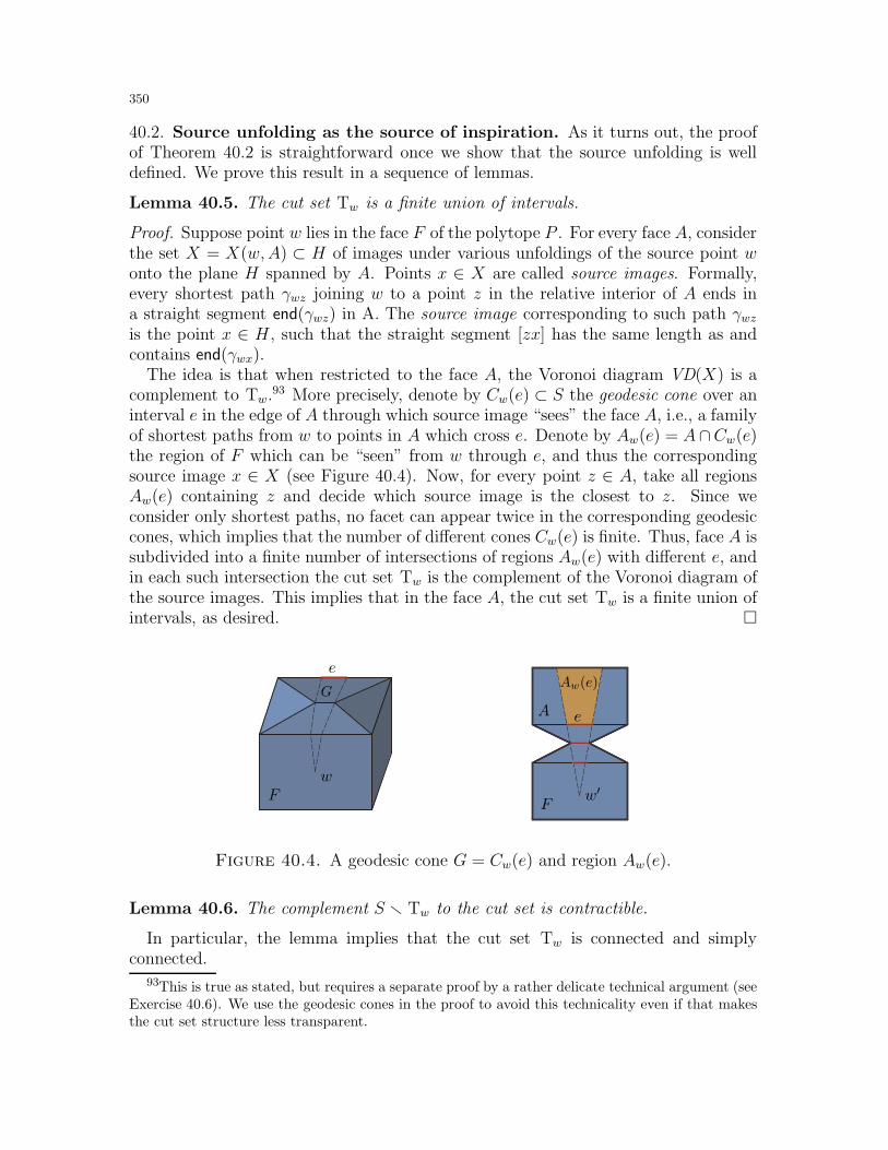
350

40.2. Source unfolding as the source of inspiration. As it turns out, the proofof Theorem 40.2 is straightforward once we show that the source unfolding is welldefined. We prove this result in a sequence of lemmas.

Lemma 40.5. The cut set Tw is a finite union of intervals.

Proof. Suppose point w lies in the face F of the polytope P . For every face A, considerthe set X = X(w,A) ⊂ H of images under various unfoldings of the source point wonto the plane H spanned by A. Points x ∈ X are called source images. Formally,every shortest path γwz joining w to a point z in the relative interior of A ends ina straight segment end(γwz) in A. The source image corresponding to such path γwzis the point x ∈ H , such that the straight segment [zx] has the same length as andcontains end(γwx).

The idea is that when restricted to the face A, the Voronoi diagram VD(X) is acomplement to Tw.93 More precisely, denote by Cw(e) ⊂ S the geodesic cone over aninterval e in the edge of A through which source image “sees” the face A, i.e., a familyof shortest paths from w to points in A which cross e. Denote by Aw(e) = A∩Cw(e)the region of F which can be “seen” from w through e, and thus the correspondingsource image x ∈ X (see Figure 40.4). Now, for every point z ∈ A, take all regionsAw(e) containing z and decide which source image is the closest to z. Since weconsider only shortest paths, no facet can appear twice in the corresponding geodesiccones, which implies that the number of different cones Cw(e) is finite. Thus, face A issubdivided into a finite number of intersections of regions Aw(e) with different e, andin each such intersection the cut set Tw is the complement of the Voronoi diagram ofthe source images. This implies that in the face A, the cut set Tw is a finite union ofintervals, as desired.

ww′

A

FF

e

e

GAw(e)

Figure 40.4. A geodesic cone G = Cw(e) and region Aw(e).

Lemma 40.6. The complement S r Tw to the cut set is contractible.

In particular, the lemma implies that the cut set Tw is connected and simplyconnected.

93This is true as stated, but requires a separate proof by a rather delicate technical argument (seeExercise 40.6). We use the geodesic cones in the proof to avoid this technicality even if that makesthe cut set structure less transparent.

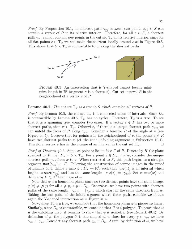
351

Proof. By Proposition 10.1, no shortest path γxy between two points x, y ∈ S cancontain a vertex of P in its relative interior. Therefore, for all z ∈ S, a shortestpath γwz cannot contain any points in the cut set Tw in its relative interior, since forall flat points c ∈ Tw we can make the shortcut locally around c as in Figure 40.5.This shows that S r Tw is contractible to w along the shortest paths.

w

v

R

γ′c

to w

to w

to z

Figure 40.5. An intersection that is Y-shaped cannot locally mini-mize length in R2 (segment γ is a shortcut). Cut set interval R in theneighborhood of a vertex v of P

Lemma 40.7. The cut set Tw is a tree in S which contains all vertices of P .

Proof. By Lemma 40.5, the cut set Tw is a connected union of intervals. Since Dw

is contractible by Lemma 40.6, Tw has no cycles. Therefore, Tw is a tree. To seethat it is a spanning tree, consider two cases. If a vertex v ∈ P has two or moreshortest paths, then w ∈ Tw. Otherwise, if there is a unique shortest path γwv, wecan unfold the faces of P along γwv. Consider a bisector R of the angle at v (seeFigure 40.5). Observe that for points z in the neighborhood of v, the points z ∈ Rhave two shortest paths to w (cf. the cone unfolding argument in Subsection 10.1).Therefore, vertex v lies in the closure of an interval in the cut set Tw.

Proof of Theorem 40.2. Suppose point w lies in face F of P . Denote by H the planespanned by F . Let Dw = S r Tw. For a point z ∈ Dw, z 6= w, consider the uniqueshortest path γwz from w to z. When restricted to F , this path begins as a straightsegment start(γwz) ⊂ F . Following the construction of source images in the proofof Lemma 40.5, define a map ϕ : Dw → R2, such that [wϕ(z)] is an interval whichbegins as start(γwz) and has the same length: |wϕ(z)| = |γwz|. Set w = ϕ(w) anddenote by U ⊂ R2 the image of ϕ.

Note that ϕ is a homeomorphism since no two distinct points have the same image:ϕ(x) 6= ϕ(y) for all x 6= y, x, y ∈ Dw. Otherwise, we have two points with shortestpaths of the same length |γxw|S = |γyw|S which start in the same direction from w.Taking the last point of the initial segment where these paths coincide we obtainagain the Y-shaped intersection as in Figure 40.5.

Now, since Tw is a tree, we conclude that the homeomorphism ϕ is piecewise linear.Similarly, since Dw is contractible, we conclude that U is a polygon. To prove that ϕis the unfolding map, it remains to show that ϕ is isometric (see Remark 40.4). Bydefinition of ϕ, the polygon U is star-shaped at w since for every y ∈ γwz we haveγwy ⊂ γwz. Consider any shortest path γxy ∈ Dw. Again, by definition of ϕ, we have

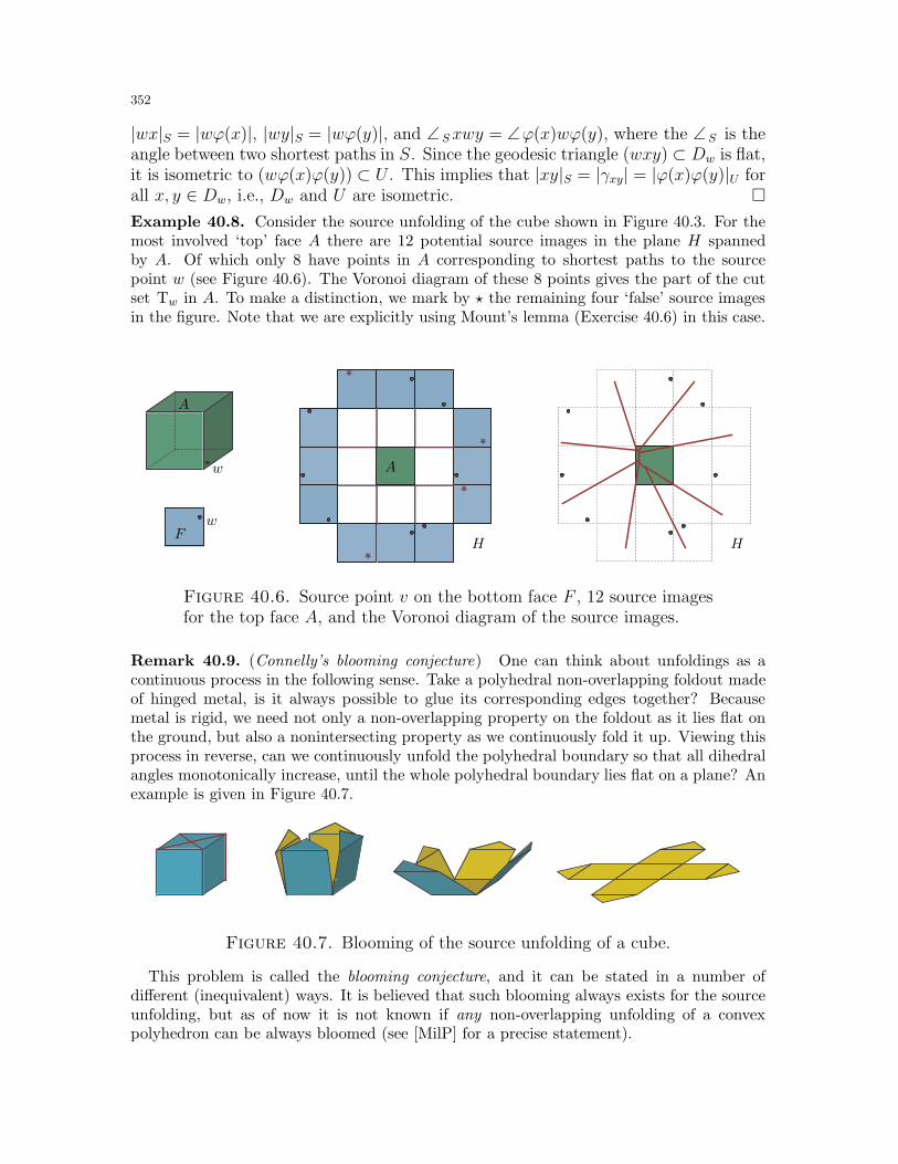
352

|wx|S = |wϕ(x)|, |wy|S = |wϕ(y)|, and ∠ Sxwy = ∠ϕ(x)wϕ(y), where the ∠ S is theangle between two shortest paths in S. Since the geodesic triangle (wxy) ⊂ Dw is flat,it is isometric to (wϕ(x)ϕ(y)) ⊂ U . This implies that |xy|S = |γxy| = |ϕ(x)ϕ(y)|U forall x, y ∈ Dw, i.e., Dw and U are isometric.

Example 40.8. Consider the source unfolding of the cube shown in Figure 40.3. For themost involved ‘top’ face A there are 12 potential source images in the plane H spannedby A. Of which only 8 have points in A corresponding to shortest paths to the sourcepoint w (see Figure 40.6). The Voronoi diagram of these 8 points gives the part of the cutset Tw in A. To make a distinction, we mark by ⋆ the remaining four ‘false’ source imagesin the figure. Note that we are explicitly using Mount’s lemma (Exercise 40.6) in this case.

*

*

*

*

w

w

A

A

FHH

Figure 40.6. Source point v on the bottom face F , 12 source imagesfor the top face A, and the Voronoi diagram of the source images.

Remark 40.9. (Connelly’s blooming conjecture) One can think about unfoldings as acontinuous process in the following sense. Take a polyhedral non-overlapping foldout madeof hinged metal, is it always possible to glue its corresponding edges together? Becausemetal is rigid, we need not only a non-overlapping property on the foldout as it lies flat onthe ground, but also a nonintersecting property as we continuously fold it up. Viewing thisprocess in reverse, can we continuously unfold the polyhedral boundary so that all dihedralangles monotonically increase, until the whole polyhedral boundary lies flat on a plane? Anexample is given in Figure 40.7.

Figure 40.7. Blooming of the source unfolding of a cube.

This problem is called the blooming conjecture, and it can be stated in a number ofdifferent (inequivalent) ways. It is believed that such blooming always exists for the sourceunfolding, but as of now it is not known if any non-overlapping unfolding of a convexpolyhedron can be always bloomed (see [MilP] for a precise statement).

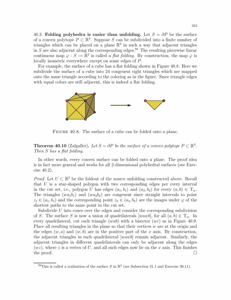
353

40.3. Folding polyhedra is easier than unfolding. Let S = ∂P be the surfaceof a convex polytope P ⊂ R3. Suppose S can be subdivided into a finite number oftriangles which can be placed on a plane R2 in such a way that adjacent trianglesin S are also adjacent along the corresponding edges.94 The resulting piecewise linearcontinuous map ϕ : S → R2 is called a flat folding. By construction, the map ϕ islocally isometric everywhere except on some edges of P .

For example, the surface of a cube has a flat folding shown in Figure 40.8. Here wesubdivide the surface of a cube into 24 congruent right triangles which are mappedonto the same triangle according to the coloring as in the figure. Since triangle edgeswith equal colors are still adjacent, this is indeed a flat folding.

Figure 40.8. The surface of a cube can be folded onto a plane.

Theorem 40.10 (Zalgaller). Let S = ∂P be the surface of a convex polytope P ⊂ R3.Then S has a flat folding.

In other words, every convex surface can be folded onto a plane. The proof ideais in fact more general and works for all 2-dimensional polyhedral surfaces (see Exer-cise 40.2).

Proof. Let U ⊂ R2 be the foldout of the source unfolding constructed above. Recallthat U is a star-shaped polygon with two corresponding edges per every intervalin the cut set, i.e., polygon U has edges (a1, b1) and (a2, b2) for every (a, b) ∈ Tw.The triangles (wa1b1) and (wa2b2) are congruent since straight intervals to pointz1 ∈ (a1, b1) and the corresponding point z2 ∈ (a2, b2) are the images under ϕ of theshortest paths to the same point in the cut set.

Subdivide U into cones over the edges and consider the corresponding subdivisionof S. The surface S is now a union of quadrilaterals [wawb], for all (a, b) ∈ Tw. Inevery quadrilateral, cut each triangle (wab) with a bisector (wc) as in Figure 40.9.Place all resulting triangles in the plane so that their vertices w are at the origin andthe edges (w, a) and (w, b) are in the positive part of the x axis. By construction,the adjacent triangles in each quadrilateral [wawb] remain adjacent. Similarly, theadjacent triangles in different quadrilaterals can only be adjacent along the edges(wz), where z is a vertex of U , and all such edges now lie on the x axis. This finishesthe proof.

94This is called a realization of the surface S in R2 (see Subsection 31.1 and Exercise 39.11).

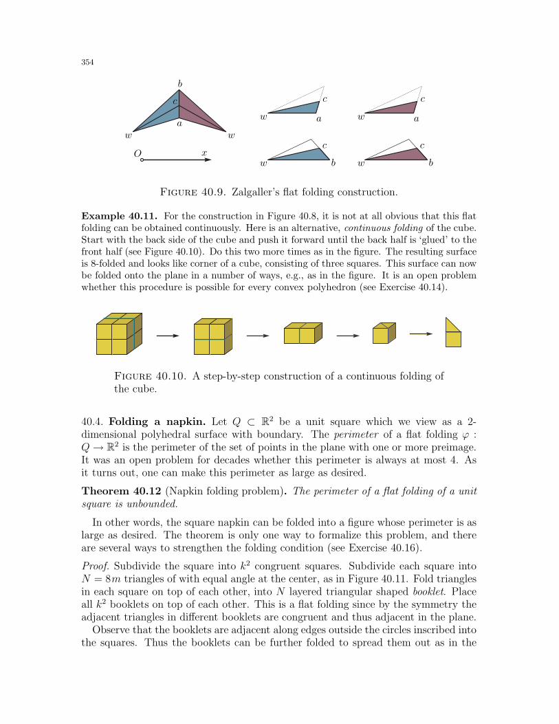
354

O xbb

b

a aa

cc

c cc

w

w

w

w

w

w

Figure 40.9. Zalgaller’s flat folding construction.

Example 40.11. For the construction in Figure 40.8, it is not at all obvious that this flatfolding can be obtained continuously. Here is an alternative, continuous folding of the cube.Start with the back side of the cube and push it forward until the back half is ‘glued’ to thefront half (see Figure 40.10). Do this two more times as in the figure. The resulting surfaceis 8-folded and looks like corner of a cube, consisting of three squares. This surface can nowbe folded onto the plane in a number of ways, e.g., as in the figure. It is an open problemwhether this procedure is possible for every convex polyhedron (see Exercise 40.14).

Figure 40.10. A step-by-step construction of a continuous folding ofthe cube.

40.4. Folding a napkin. Let Q ⊂ R2 be a unit square which we view as a 2-dimensional polyhedral surface with boundary. The perimeter of a flat folding ϕ :Q→ R2 is the perimeter of the set of points in the plane with one or more preimage.It was an open problem for decades whether this perimeter is always at most 4. Asit turns out, one can make this perimeter as large as desired.

Theorem 40.12 (Napkin folding problem). The perimeter of a flat folding of a unitsquare is unbounded.

In other words, the square napkin can be folded into a figure whose perimeter is aslarge as desired. The theorem is only one way to formalize this problem, and thereare several ways to strengthen the folding condition (see Exercise 40.16).

Proof. Subdivide the square into k2 congruent squares. Subdivide each square intoN = 8m triangles of with equal angle at the center, as in Figure 40.11. Fold trianglesin each square on top of each other, into N layered triangular shaped booklet. Placeall k2 booklets on top of each other. This is a flat folding since by the symmetry theadjacent triangles in different booklets are congruent and thus adjacent in the plane.

Observe that the booklets are adjacent along edges outside the circles inscribed intothe squares. Thus the booklets can be further folded to spread them out as in the

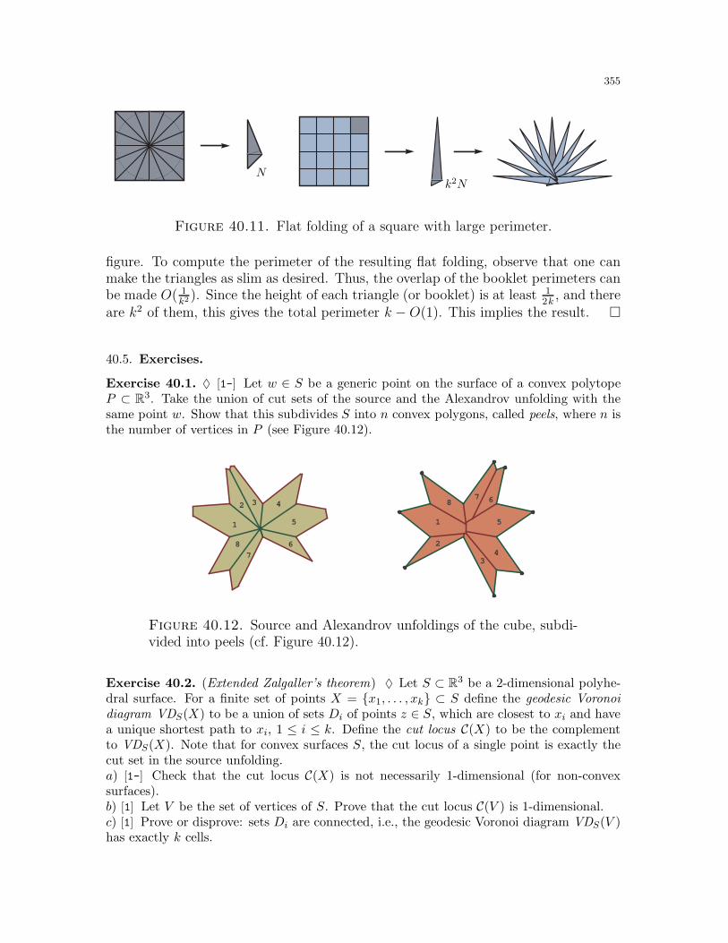
355

Nk2N

Figure 40.11. Flat folding of a square with large perimeter.

figure. To compute the perimeter of the resulting flat folding, observe that one canmake the triangles as slim as desired. Thus, the overlap of the booklet perimeters canbe made O( 1

k2 ). Since the height of each triangle (or booklet) is at least 12k

, and thereare k2 of them, this gives the total perimeter k − O(1). This implies the result.

40.5. Exercises.

Exercise 40.1. ♦ [1-] Let w ∈ S be a generic point on the surface of a convex polytopeP ⊂ R3. Take the union of cut sets of the source and the Alexandrov unfolding with thesame point w. Show that this subdivides S into n convex polygons, called peels, where n isthe number of vertices in P (see Figure 40.12).

1

2 4

5

6

7

8

3

1

2

3

4

87

6

5

Figure 40.12. Source and Alexandrov unfoldings of the cube, subdi-vided into peels (cf. Figure 40.12).

Exercise 40.2. (Extended Zalgaller’s theorem) ♦ Let S ⊂ R3 be a 2-dimensional polyhe-dral surface. For a finite set of points X = x1, . . . , xk ⊂ S define the geodesic Voronoidiagram VDS(X) to be a union of sets Di of points z ∈ S, which are closest to xi and havea unique shortest path to xi, 1 ≤ i ≤ k. Define the cut locus C(X) to be the complementto VDS(X). Note that for convex surfaces S, the cut locus of a single point is exactly thecut set in the source unfolding.a) [1-] Check that the cut locus C(X) is not necessarily 1-dimensional (for non-convexsurfaces).b) [1] Let V be the set of vertices of S. Prove that the cut locus C(V ) is 1-dimensional.c) [1] Prove or disprove: sets Di are connected, i.e., the geodesic Voronoi diagram VDS(V )has exactly k cells.

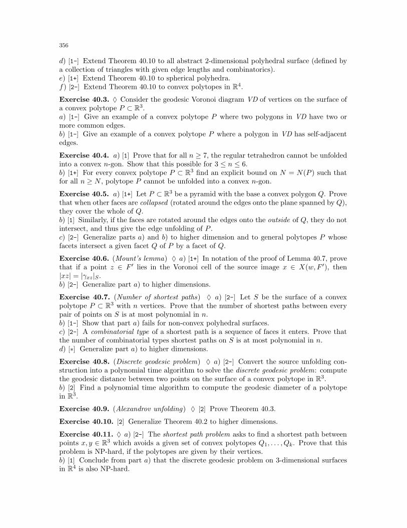
356

d) [1-] Extend Theorem 40.10 to all abstract 2-dimensional polyhedral surface (defined bya collection of triangles with given edge lengths and combinatorics).e) [1+] Extend Theorem 40.10 to spherical polyhedra.f) [2-] Extend Theorem 40.10 to convex polytopes in R4.

Exercise 40.3. ♦ Consider the geodesic Voronoi diagram VD of vertices on the surface ofa convex polytope P ⊂ R3.a) [1-] Give an example of a convex polytope P where two polygons in VD have two ormore common edges.b) [1-] Give an example of a convex polytope P where a polygon in VD has self-adjacentedges.

Exercise 40.4. a) [1] Prove that for all n ≥ 7, the regular tetrahedron cannot be unfoldedinto a convex n-gon. Show that this possible for 3 ≤ n ≤ 6.b) [1+] For every convex polytope P ⊂ R3 find an explicit bound on N = N(P ) such thatfor all n ≥ N , polytope P cannot be unfolded into a convex n-gon.

Exercise 40.5. a) [1+] Let P ⊂ R3 be a pyramid with the base a convex polygon Q. Provethat when other faces are collapsed (rotated around the edges onto the plane spanned by Q),they cover the whole of Q.b) [1] Similarly, if the faces are rotated around the edges onto the outside of Q, they do notintersect, and thus give the edge unfolding of P .c) [2-] Generalize parts a) and b) to higher dimension and to general polytopes P whosefacets intersect a given facet Q of P by a facet of Q.

Exercise 40.6. (Mount’s lemma) ♦ a) [1+] In notation of the proof of Lemma 40.7, provethat if a point z ∈ F ′ lies in the Voronoi cell of the source image x ∈ X(w,F ′), then|xz| = |γxz|S .b) [2-] Generalize part a) to higher dimensions.

Exercise 40.7. (Number of shortest paths) ♦ a) [2-] Let S be the surface of a convexpolytope P ⊂ R3 with n vertices. Prove that the number of shortest paths between everypair of points on S is at most polynomial in n.b) [1-] Show that part a) fails for non-convex polyhedral surfaces.c) [2-] A combinatorial type of a shortest path is a sequence of faces it enters. Prove thatthe number of combinatorial types shortest paths on S is at most polynomial in n.d) [∗] Generalize part a) to higher dimensions.

Exercise 40.8. (Discrete geodesic problem) ♦ a) [2-] Convert the source unfolding con-struction into a polynomial time algorithm to solve the discrete geodesic problem: computethe geodesic distance between two points on the surface of a convex polytope in R3.b) [2] Find a polynomial time algorithm to compute the geodesic diameter of a polytopein R3.

Exercise 40.9. (Alexandrov unfolding) ♦ [2] Prove Theorem 40.3.

Exercise 40.10. [2] Generalize Theorem 40.2 to higher dimensions.

Exercise 40.11. ♦ a) [2-] The shortest path problem asks to find a shortest path betweenpoints x, y ∈ R3 which avoids a given set of convex polytopes Q1, . . . , Qk. Prove that thisproblem is NP-hard, if the polytopes are given by their vertices.b) [1] Conclude from part a) that the discrete geodesic problem on 3-dimensional surfacesin R4 is also NP-hard.

357

Exercise 40.12. Let S = ∂P be the surface of a convex polytope, and let γ = γxy be ashortest path between some two points x, y ∈ S.a) [1] For every ε > 0, give a construction of P , such that for some shortest path γ we havefor the total curvature: κ(γ) > 2π − ε.b) [2] Give a construction of P , such that for some shortest path γ we have for the totalcurvature: κ(γ) > 2π.c) [2-] Define the folding angle υ(γ) to be the sum of exterior angles of edges of P intersectedby γ. Check that υ(γ) ≥ κ(γ). Show that υ(γ) is unbounded, i.e., for every N > 0 give aconstruction of P and γ, such that υ(γ) > N .d) [∗] Prove or disprove: κ(γ) is bounded for all P and γ.

Exercise 40.13. (Volkov) Let S = ∂P be the surface of a convex cap P ⊂ R3 (seeSubsection 25.6). Suppose x, y ∈ S are two points in the bounded faces of S.a) [1+] Prove that the length of all geodesics between x and y is bounded.b) [2-] Conclude that there is at most a finite number of geodesics between x and y.

Exercise 40.14. ♦ a) [1-] Formalize the continuous folding introduced in Example 40.11.Show that there exists a continuous folding which produces the folding in Figure 40.8.b) [1-] Find a continuous folding of the truncated cube (see Figure 16.4).c) [1] Find a continuous folding of the regular icosahedron and the regular dodecahedron.d) [1] Prove that every tetrahedron has a continuous folding.e) [1+] Show that every convex surface has a continuous folding.

Exercise 40.15. Let S = ∂P be the surface of a convex polytope in R3. Define a layeredfolding to be a flat folding map ϕ : S → R2 with the ordering map π : S → N defined sothat adjacent triangles in the layers can be physically glued together.a) [1-] Formalize the definition. Check that every continuous folding of S gives a layeredfolding.b) [1+] Prove that every S as above has a layered folding.c) [1+] Generalize b) to abstract 2-dimensional polyhedral surfaces homeomorphic to asphere.

Exercise 40.16. (Napkin problem) ♦ a) [1] Define the reflection folding of a polygon tobe a flat folding obtained sequentially, by reflecting the whole polygon along a line (ab) as inFigure 40.13. Show that the perimeter does not increase under these reflections. Concludethat the perimeter of every reflection folding of a napkin is at most 4.b) [∗] Define a natural folding of a polygon to be a flat folding obtain sequentially, byreflecting layers along a line (see Figure 40.13). Show that every natural folding of a unitsquare has perimeter at most 4.c) [1+] Find a layered folding (see Example 40.15) of a unit square with perimeter as largeas desired.d) [2-] Same for continuous foldings (see Example 40.11).e) [2] Same for continuous piecewise linear foldings.

Exercise 40.17. a) [1-] Find a non-convex polytope P in R3 which does not have a non-overlapping unfolding.b) [1+] Same for P with convex faces.

Exercise 40.18. [∗] Prove Durer’s conjecture for zonotopes (see Exercise 7.16).

Exercise 40.19. [∗] Prove that every star-shaped surface in R3 has a (general) non-overlapping unfolding.

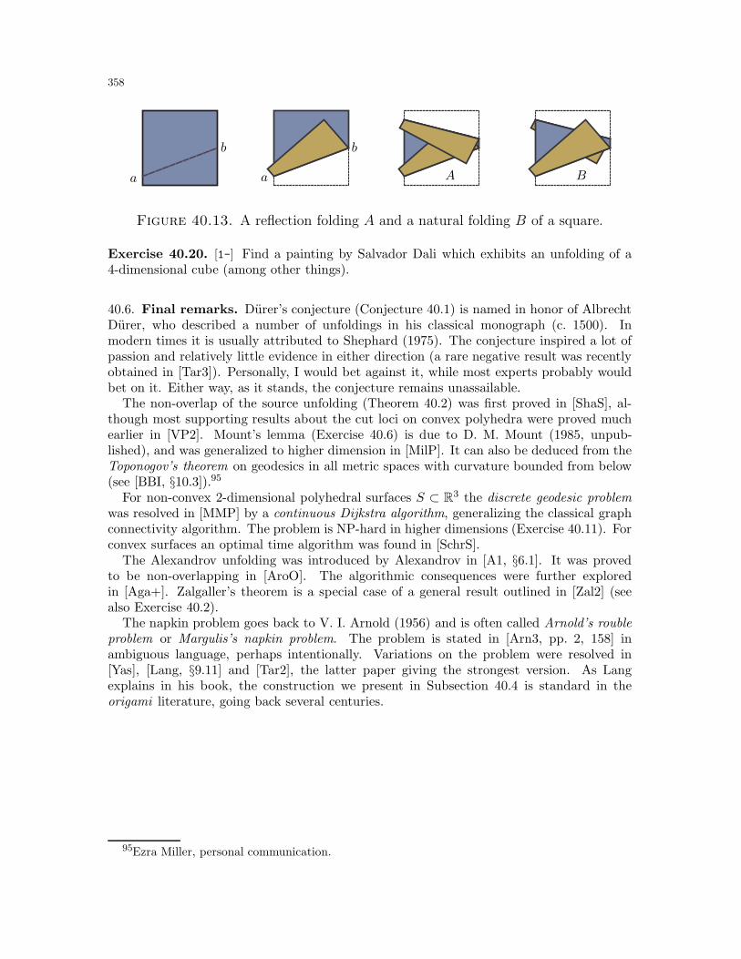
358

aa

bb

A B

Figure 40.13. A reflection folding A and a natural folding B of a square.

Exercise 40.20. [1-] Find a painting by Salvador Dali which exhibits an unfolding of a4-dimensional cube (among other things).

40.6. Final remarks. Durer’s conjecture (Conjecture 40.1) is named in honor of AlbrechtDurer, who described a number of unfoldings in his classical monograph (c. 1500). Inmodern times it is usually attributed to Shephard (1975). The conjecture inspired a lot ofpassion and relatively little evidence in either direction (a rare negative result was recentlyobtained in [Tar3]). Personally, I would bet against it, while most experts probably wouldbet on it. Either way, as it stands, the conjecture remains unassailable.

The non-overlap of the source unfolding (Theorem 40.2) was first proved in [ShaS], al-though most supporting results about the cut loci on convex polyhedra were proved muchearlier in [VP2]. Mount’s lemma (Exercise 40.6) is due to D. M. Mount (1985, unpub-lished), and was generalized to higher dimension in [MilP]. It can also be deduced from theToponogov’s theorem on geodesics in all metric spaces with curvature bounded from below(see [BBI, §10.3]).95

For non-convex 2-dimensional polyhedral surfaces S ⊂ R3 the discrete geodesic problemwas resolved in [MMP] by a continuous Dijkstra algorithm, generalizing the classical graphconnectivity algorithm. The problem is NP-hard in higher dimensions (Exercise 40.11). Forconvex surfaces an optimal time algorithm was found in [SchrS].

The Alexandrov unfolding was introduced by Alexandrov in [A1, §6.1]. It was provedto be non-overlapping in [AroO]. The algorithmic consequences were further exploredin [Aga+]. Zalgaller’s theorem is a special case of a general result outlined in [Zal2] (seealso Exercise 40.2).

The napkin problem goes back to V. I. Arnold (1956) and is often called Arnold’s roubleproblem or Margulis’s napkin problem. The problem is stated in [Arn3, pp. 2, 158] inambiguous language, perhaps intentionally. Variations on the problem were resolved in[Yas], [Lang, §9.11] and [Tar2], the latter paper giving the strongest version. As Langexplains in his book, the construction we present in Subsection 40.4 is standard in theorigami literature, going back several centuries.

95Ezra Miller, personal communication.

359

Part III

Details, details...

360

41. Appendix

41.1. The area of spherical polygons. In the next two subsections we present severalbasic definitions and classical results in spherical geometry. A few preliminary words. Weconsider a unit sphere S2 with center at the origin O. The role of lines play great circles,defined as circles of radius 1 with centers at the origin O. Triangles, polygons, areas, etc.are defined by analogy with the plane geometry. The angle between two ‘lines’ is defined asthe dihedral angle between planes containing the corresponding great circles. Finally, recallthat area(S2) = 4π.

Theorem 41.1 (Girard’s formula). Let T be a spherical triangle with angles α, β and γ.Then area(T ) = α+ β + γ − π.

Proof. Let A,B and C be the triangular regions attached to the triangle as in Figure 41.1.Observe that area(A∪ T ) = α

2π × area(S2) = 2α, area(B ∪ T ) = 2β, and area(C ∪ T ) = 2γ.Now for the upper hemisphere H we have:

area(H) = area(A) + area(B) + area(C ′) + area(T ) =(area(A) + area(T )

)

+(area(A) + area(T )

)+(area(C) + area(T )

)− 2 area(T )

= 2(α+ β + γ − area(T )

)

On the other hand, area(H) = area(S)/2 = 2π, which implies the result.

α β

γ

AB

C

C ′

T α

cb

a

x

y

z

O

u v

S2S2

Figure 41.1. The area and the law of cosines for spherical triangles.

Theorem 41.2 (The area of a spherical polygon). Let Q be a spherical n-gon with anglesα1, . . . , αn. Then area(Q) = α1 + . . .+ αn − (n− 2)π.

We refer to the formula in the theorem as Girard’s formula for polygons. For the proof,subdivide the polygon into triangles and sum the areas of all triangles according to Girard’sformula. The details are straightforward.

41.2. The law of cosines for spherical triangles. In Section 21 we repeatedly use thefollowing claim: if the spherical triangles (xyz) and (x′y′z′) satisfy |xy| = |x′y′|, |xz| = |x′z′|,and ∢ yxz > ∢ y′x′z′, then |yz| > |y′z′|. In the plane this follows immediately from the(first) law of cosines:

|yz|2 = |xy|2 + |xz|2 − 2 |xy| |xz| cos yxz.

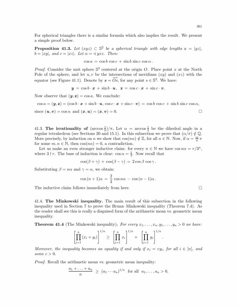
361

For spherical triangles there is a similar formula which also implies the result. We presenta simple proof below.

Proposition 41.3. Let (xyz) ⊂ S2 be a spherical triangle with edge lengths a = |yz|,b = |xy|, and c = |xz|. Let α = ∢ yxz. Then:

cos a = cos b cos c + sin b sin c cosα .

Proof. Consider the unit sphere S2 centered at the origin O. Place point x at the NorthPole of the sphere, and let u, v be the intersections of meridians (xy) and (xz) with the

equator (see Figure 41.1). Denote by s =−→Os, for any point s ∈ S2. We have:

y = cos b · x + sin b · u , z = cos c · x + sin c · v .Now observe that (y , z) = cos a. We conclude:

cos a = (y , z) = (cos b · x + sin b · u , cos c · x + sin c · v) = cos b cos c + sin b sin c cosα,

since (u , v ) = cosα and (x ,u) = (x , v ) = 0.

41.3. The irrationality of (arccos 13)/π. Let α = arccos 1

3 be the dihedral angle in aregular tetrahedron (see Sections 20 and 15.1). In this subsection we prove that (α/π) /∈ Q.More precisely, by induction on n we show that cos(nα) /∈ Z, for all n ∈ N. Now, if α = m

n πfor some m,n ∈ N, then cos(nα) = 0, a contradiction.

Let us make an even stronger inductive claim: for every n ∈ N we have cosnα = r/3n,where 3 ∤ r. The base of induction is clear: cosα = 1

3 . Now recall that

cos(β + γ) + cos(β − γ) = 2 cos β cos γ .

Substituting β = nα and γ = α, we obtain:

cos (n+ 1)α =2

3cosnα − cos (n− 1)α .

The inductive claim follows immediately from here.

41.4. The Minkowski inequality. The main result of this subsection in the followinginequality used in Section 7 to prove the Brunn–Minkowski inequality (Theorem 7.4). Asthe reader shall see this is really a disguised form of the arithmetic mean vs. geometric meaninequality.

Theorem 41.4 (The Minkowski inequality). For every x1, . . . , xn, y1, . . . , yn > 0 we have:

[n∏

i=1

(xi + yi)

]1/n

≥[n∏

i=1

xi

]1/n

+

[n∏

i=1

yi

]1/n

.

Moreover, the inequality becomes an equality if and only if xi = cyi, for all i ∈ [n], andsome c > 0.

Proof. Recall the arithmetic mean vs. geometric mean inequality:

a1 + . . .+ ann

≥ (a1 · · · an)1/n for all a1, . . . , an > 0,

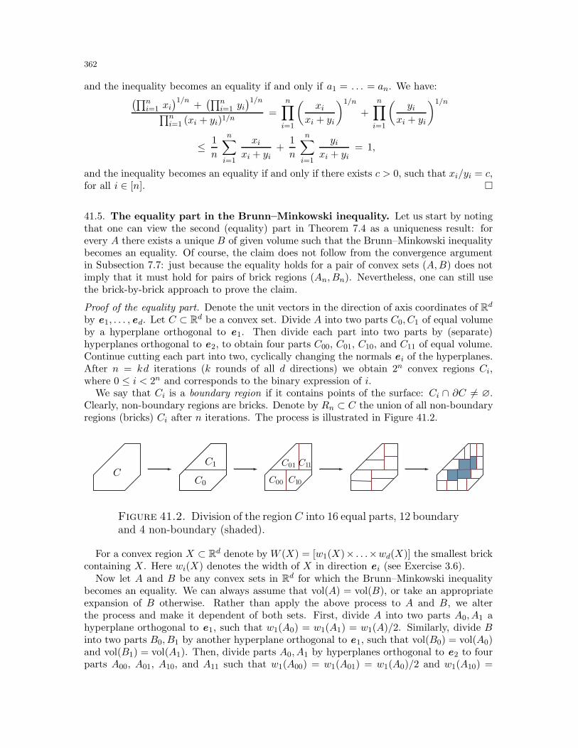
362

and the inequality becomes an equality if and only if a1 = . . . = an. We have:(∏n

i=1 xi)1/n

+(∏n

i=1 yi)1/n

∏ni=1 (xi + yi)1/n

=

n∏

i=1

(xi

xi + yi

)1/n

+

n∏

i=1

(yi

xi + yi

)1/n

≤ 1

n

n∑

i=1

xixi + yi

+1

n

n∑

i=1

yixi + yi

= 1,

and the inequality becomes an equality if and only if there exists c > 0, such that xi/yi = c,for all i ∈ [n].

41.5. The equality part in the Brunn–Minkowski inequality. Let us start by notingthat one can view the second (equality) part in Theorem 7.4 as a uniqueness result: forevery A there exists a unique B of given volume such that the Brunn–Minkowski inequalitybecomes an equality. Of course, the claim does not follow from the convergence argumentin Subsection 7.7: just because the equality holds for a pair of convex sets (A,B) does notimply that it must hold for pairs of brick regions (An, Bn). Nevertheless, one can still usethe brick-by-brick approach to prove the claim.

Proof of the equality part. Denote the unit vectors in the direction of axis coordinates of Rd

by e1, . . . , ed. Let C ⊂ Rd be a convex set. Divide A into two parts C0, C1 of equal volumeby a hyperplane orthogonal to e1. Then divide each part into two parts by (separate)hyperplanes orthogonal to e2, to obtain four parts C00, C01, C10, and C11 of equal volume.Continue cutting each part into two, cyclically changing the normals e i of the hyperplanes.After n = kd iterations (k rounds of all d directions) we obtain 2n convex regions Ci,where 0 ≤ i < 2n and corresponds to the binary expression of i.

We say that Ci is a boundary region if it contains points of the surface: Ci ∩ ∂C 6= ∅.Clearly, non-boundary regions are bricks. Denote by Rn ⊂ C the union of all non-boundaryregions (bricks) Ci after n iterations. The process is illustrated in Figure 41.2.

CC0

C1

C00

C01

C10

C11

Figure 41.2. Division of the region C into 16 equal parts, 12 boundaryand 4 non-boundary (shaded).

For a convex region X ⊂ Rd denote by W (X) = [w1(X)× . . .×wd(X)] the smallest brickcontaining X. Here wi(X) denotes the width of X in direction e i (see Exercise 3.6).

Now let A and B be any convex sets in Rd for which the Brunn–Minkowski inequalitybecomes an equality. We can always assume that vol(A) = vol(B), or take an appropriateexpansion of B otherwise. Rather than apply the above process to A and B, we alterthe process and make it dependent of both sets. First, divide A into two parts A0, A1 ahyperplane orthogonal to e1, such that w1(A0) = w1(A1) = w1(A)/2. Similarly, divide Binto two parts B0, B1 by another hyperplane orthogonal to e1, such that vol(B0) = vol(A0)and vol(B1) = vol(A1). Then, divide parts A0, A1 by hyperplanes orthogonal to e2 to fourparts A00, A01, A10, and A11 such that w1(A00) = w1(A01) = w1(A0)/2 and w1(A10) =

363

w1(A11) = w1(A1)/2. Then divide sets B0, B1 by hyperplanes into four parts B00, B01, B10,and B11, such that the corresponding sets in A and B have equal volume. Then repeat thisiteration of cuts for e3,. . . ,ed, making a total of d iterations of cuts. Then switch the rolesof A and B and in the next d cuts halve the widths of regions in B. This make the totalof 2d cut, which we call a round. Now make k rounds of such cuts. In the notation above,we obtain regions Ai and Bi, 0 ≤ i < 2n, where n = 2kd.

Denote by Xn and Yn the unions of all non-boundary regions Ai and Bi, respectively.Clearly, there may be regions in Xn that do not have corresponding regions in Yn and viceversa. Let X ′

n ⊂ Xn be a union of non-boundary regions Ai such that the region Bi is alsonon-boundary. Define Y ′

n ⊂ Yn analogously. A priori X ′n and Y ′

n can be disconnected, solet X∗

n, Y∗n be their connected components containing centers of mass cm(A) and cm(B),

respectively.Observe that after k rounds of cuts as above we have wr(Ai) ≤ wr(A)/2k ≤ diam(A)/2k.

Letting D = maxdiam(A),diam(B) we conclude that wr(Ai), wr(Bi) ≤ ε, where ε =(D/2k) > 0. For large enough k = n/2d we can ensure that neither center of mass lies in aboundary region. Further,

vol(X∗n) ≥ vol(A) − [ε · area(A)],

and thus vol(X∗n), vol(Y ∗

n )→ vol(A) = vol(B) as n→∞.Let us further restrict our regions: denote by X

n and Y n the union of bricks which

have no points at distance ≤ ε from the boundary, where ε > 0 is as above. From thereasoning as above, for large enough n we obtained two connected brick regions X

n, Yn

with corresponding bricks Ai ⊂ A, Bi ⊂ B, and such that Xn → A, Y

n → B, as n→∞.

Now comes the key observation. In the inductive step in the proof of the Brunn–Minkowski inequality in Section 7, we divided the regions A,B into two disjoint parts by ahyperplane in the same ratio, and concluded that the inequality holds for sets A,B only if itholds for the corresponding parts. Clearly, the equality also holds only if the equality holdsfor the corresponding parts. Repeating the procedure we get again the equality for the fourcorresponding pairs of smaller parts, etc. By induction, we conclude that the equality inthe Brunn–Minkowski inequality holds for all pairs (Ai, Bi), 0 ≤ i < 2n.

Now, if both Ai and Bi are bricks the equality can hold only if one is an expansion ofthe other. Since vol(Ai) = vol(Bi) by construction, bricks Ai, Bi must be equal up to atranslation. By itself, this does not imply that X

n and Y n are equal. It does, however,

imply that they are converging to the same convex set, by the following argument.We say that two bricks Ai and Ai′ touch each other if their boundaries intersect in points

interior to the faces. Observe that the corresponding bricks Bi and Bi′ do not necessarilyhave to touch, but they must both touch a hyperplane separating them, a hyperplanecorresponding to a hyperplane separating Ai and A′

i.Denote by Aj and Bj, 0 ≤ j < 2d, the regions resulted after the first round of cuts.

Consider Aj = Aj ∩ X

n and Bj = Bj ∩ Y

n . Both brick regions contain a large numberof smaller regions, but none of them boundary regions. Furthermore, since point of theboundary region can lie in an interval parallel to er between two points in A

j or in Bj .

Now, we claim that Aj ≃ B

j for all j. In other words, these regions can be obtainedfrom each other by a translation. Indeed, start at a corner which must contain equalcorresponding bricks. Start adding bricks along the straight interior edges of A

j , and all ofthem will sequentially touch each other. Thus, the interior edges of B

j will be lined up withequal corresponding bricks. Now start filling all 2-dimensional interior faces in A

j and Bj ,

again by the equal corresponding bricks, etc. Eventually we obtain two equal fillings of the

364

regions, implying that the regions themselves are equal. Note that we are implicitly usingthe fact that by convexity of A,B and the construction, there are no ‘holes’ in A

j , Bj .

While the corresponding regionsAj , B

j are equal, we can no longer use the same argument

to prove that Xn = Y

n . Instead, let us put them together in the reverse order they wereobtained by separation with hyperplanes. When put together, regions A

j and Bj can be

shifted along the axes. Observe that by convexity of A and B, they cannot be shifted bymore than (2ε) in each direction. Thus in fact the distance between the corresponding

points in Xn, Y

n is at most

√d (2ε)→ 0 as n→∞.

Make a translation of Y n so that it has the came center of mass as X

n. From above,we have vol(Y

n r Xn) → 0. Since X

n → A and Y n → B, this implies that A ≃ B, and

completes the proof.

41.6. The Cayley–Menger determinant. Here we give an explicit computation of theCayley–Menger determinant defined and studied in Section 34. This is an important ingre-dient in the proof of the bellows conjecture (Theorem 31.2).

Theorem 34.5 (Cayley–Menger). For every simplex ∆ = (v0v1 . . . vd) ⊂ Rd, we have:

vol2(∆) =(−1)d−1

2d d!2· det

0 1 1 1 . . . 11 0 ℓ201 ℓ202 . . . ℓ20d1 ℓ201 0 ℓ212 . . . ℓ21d1 ℓ202 ℓ212 0 . . . ℓ22d...

......

.... . .

...1 ℓ20d ℓ21d ℓ22d . . . 0

,

where ℓij = |vivj |, for all 0 ≤ i < j ≤ d.

Proof of Theorem 34.5. Suppose vi = (xi1, . . . , xid) ∈ Rd, for all 0 ≤ i ≤ d. Define matri-ces A and B as follows:

A =

x01 x02 . . . x0d 1x11 x12 . . . x1d 1

......

. . ....

...xd1 xd2 . . . xdd 1

, B =

x01 x02 . . . x0d 0x11 x12 . . . x1d 0

......

. . ....

...xd1 xd2 . . . xdd 0

.

Clearly, det(B) = 0, and

det(A) = det

x01 x02 . . . x0d 1x11 − x01 x12 − x02 . . . x1d − x0d 0

......

. . ....

...xd1 − x01 xd2 − x02 . . . xdd − x0d 0

= (−1)d d! vol(∆).

Note that

A · AT =(〈vi, vj〉+ 1

)0≤i,j≤d , and B · BT =

(〈vi, vj〉

)0≤i,j≤d .

365

From here we have:

det(A · AT ) = det

〈v0, v0〉+ 1 〈v0, v1〉+ 1 . . . 〈v0, vd〉+ 1 0〈v1, v0〉+ 1 〈v1, v1〉+ 1 . . . 〈v1, vd〉+ 1 0

......

. . ....

...〈vd, v0〉+ 1 〈vd, v1〉+ 1 . . . 〈vd, vd〉+ 1 0

1 1 . . . 1 1

= − det

〈v0, v0〉 〈v0, v1〉 . . . 〈v0, vd〉 1〈v1, v0〉 〈v1, v1〉 . . . 〈v1, vd〉 1

......

. . ....

...〈vd, v0〉 〈vd, v1〉 . . . 〈vd, vd〉 1

1 1 . . . 1 −1

.

Since det(〈vi, vj〉

)= det(B · BT ) = det2(B) = 0, in the determinant above we can replace

the bottom right entry −1 with 0. Denote the resulting matrix by M .Now observe that ℓ2ij = 〈vi, vi〉 − 2〈vi, vj〉 + 〈vj , vj〉. Denote by C the matrix as in the

theorem. Using row and column operations we obtain:

det(C) = det

−2〈v0, v0〉 −2〈v0, v1〉 . . . −2〈v0, vd〉 1−2〈v1, v0〉 −2〈v1, v1〉 . . . −2〈v1, vd〉 1

......

. . ....

...−2〈vd, v0〉 −2〈vd, v1〉 . . . −2〈vd, vd〉 1

1 1 . . . 1 0

= (−2)d det(M).

Since det(M) = − det(A ·AT ) = −(d! vol(∆)

)2, we conclude that

det(C) = (−1)d−1 2d d!2 vol2(∆),

as desired.

41.7. The theory of places. The proof of the bellows conjecture (Theorem 31.2) is basedon the integrality criteria (Theorem 34.2), a classical result in the theory of places. In thissection we present a reworking of the presentation in [Lan], making it self-contained and,hopefully, more accessible to the reader unfamiliar with the field.

Let L be a field containing ring R. We will always assume that R contains 1. To provethe integrality criteria we need to show:

A. if x ∈ L is integral over R, then every place that is finite over R, is also finiteover x;

B. if x ∈ L is not integral over R, then there exists a place that is finite over R,and infinite over x.

While the proof of the bellows conjecture uses only part B, we include a simple proof ofpart A for the sake of clarity and completeness.

Proof of part A. Since x ∈ L is integral over R, by definition we have

xn + an−1xn−1 + . . .+ a1x + a0 = 0 ,

where ai ∈ R. Dividing both sides by xn we obtain:

1 +an−1

x+ . . . +

a1

xn−1+

a0

xn= 0 .

366

Recall that F = F ∪ ∞ and let ϕ : L → F be a place which is finite on R. Supposethat ϕ(x) =∞. Then ϕ( 1

x ) = 0. Applying ϕ to both sides of the above equation, we obtain1 = 0, a contradiction.

Proof of part B. Since x is not integral over R, we have x 6= 0. Let us construct a place

ϕ : L → F , for some (possibly very large) field F , such that ϕ( 1x ) = 0. This would imply

that ϕ(x) =∞ and prove the claim.Denote by R〈 1x〉 the ring generated by R and 1

x . Consider the ideal I = 1xR〈 1x〉 generated

by 1x . Note that I 6= R〈 1x〉. Indeed, otherwise 1 ∈ 1

xR〈 1x〉 and we can write

1 =a1

x+a2

x2+ . . . +

anxn

,

for some ai ∈ R. Multiplying both sides by xn gives a monic polynomial equation for x,implying that x is integral over R, a contradiction.

From above, there exists a maximal ideal m ⊂ R〈 1x〉 containing I. Since m is a maximal

ideal, we can consider a field F1 = R〈 1x〉/m. This defines a natural map ϕ : R〈 1x〉 → F1,

such that ϕ( 1x) = 0. Denote by F the algebraic closure of F1. Let us extend the map ϕ

from F1 to F , still calling it ϕ. We have ϕ : R〈 1x〉 → F . 96

Now, consider a set of ring homomorphisms ψS : S → F such that R〈 1x〉 ⊂ S L,

and ψS(y) = ϕ(y) for all y ∈ R〈 1x〉. There is a natural partial order ψS < ψS′ on thesehomomorphisms, where S ⊂ S′ and ψS′ is an extension of ψS .

Consider an increasing sequence of ring homomorphisms ψ1 < ψ2 < . . . < ψi < . . .,corresponding to an increasing sequence of rings R〈 1x〉 ⊂ S1 ⊂ S2 ⊂ . . . ⊂ Si ⊂ . . ., whereSi L. We can construct a ring S = ∪iSi and a homomorphism ψ : S → F , whereψi < ψ for all i = 1, 2, . . . Clearly, S L, since if S = L then x ∈ Si for some i, and1 = ϕ(1) = ϕ(x · 1

x) 6= ϕ(x) · ϕ( 1x) = 0. Therefore, homomorphism ψ is an upper bound

on ψi. Clearly, the same argument works for all infinite chains of homomorphisms (notnecessarily countable), and by Zorn’s lemma the partial order defined above has a maximalelement, i.e., a homomorphism which cannot be extended.

The following lemma characterizing the ring of the maximal homomorphism is the keyresult which allows us to finish the construction. We postpone the proof of the lemma untilthe end of the proof of the theorem.

Lemma 41.5. Let ψ : S → F be a maximal homomorphism, where ϕ < ψ and R〈 1x〉 ⊂S L. Then for every y ∈ L either y ∈ S or 1

y ∈ S.

We can now define ψ : L→ F by letting ψ(y) = ψ(s) for all y ∈ S, and ψ(y) =∞ for ally /∈ S. Since S L is a subring, it is easy to see (by checking all relations in the definitionof a place) that

(⊖) ψ

(1

y

)= 0 for all y /∈ S

implies that ψ is a place. Therefore, to prove part B it suffice to establish (⊖).By the lemma, for every y /∈ S we have 1

y ∈ S. Now suppose that ψ( 1y ) 6= 0. Take a

bigger ring S′ = S〈y〉 generated by S and y, with a homomorphism ψ′ : S′ → F definedby ψ′(y) = 1/ψ( 1

y ) and ψ′(s) = ϕ(s), for all s ∈ S. To see that the map ψ′ is indeed a

ring homomorphism, simply note that∑n

i=0 siyi = 0 is equivalent to

∑ni=0 si(

1y )n−i = 0,

96The importance of taking the algebraic closure F ⊃ F1 will come only at the end of the proofof Lemma 41.5. Until then, the arguments work for any extension of F1.

367

for all si ∈ S. Since y ∈ S′, we conclude that ψ < ψ′, a contradiction with ψ beingmaximal. Therefore, ψ( 1

y ) = 0 and we proved (⊖). This completes the proof of part B

modulo Lemma 41.5.

Proof of Lemma 41.5. Suppose y, 1y /∈ S for some y ∈ L. Define S1 = S〈y〉 and S2 = S〈 1y 〉.

We obtain a contradiction with maximality of ψ : S → F by showing that ψ can be extendedto at least one of the rings S1 or S2.

Let m = Ker(ψ : S → F ) ⊂ S be the ideal of elements mapped into 0 ∈ F . Let us startwith the following two technical lemmas whose proofs we postpone.

Sublemma 41.6. The ideal m⊂ S is maximal. In addition, for every y /∈m, we have1y ∈ S.97

Sublemma 41.7. Either mS1 6= S1 or mS2 6= S2.

By Sublemma 41.6, the ideal m ⊂ S is maximal and S/m is a field. Thus, we obtaina natural field homomorphism ψ : S/m → F . By Sublemma 41.7, we can assume thatmS1 S1.

Since mS1 is an ideal in S1, we can consider a maximal ideal m1 ⊃ m in S1. Then S1/m1

is a field extension of S/m, obtained by adding α = y, defined as the class of y. Note herethat this implies that α is algebraic over S/m, since otherwise S1/m1 = S/m[α] is not afield.

Now, to prove the lemma it suffices to construct an extension ψ1 : S1/m1 → F of ψ,since this would give a ring homomorphism ψ1 : S1 → F by letting ψ1 : m1 → 0. Thiswould imply that ψ < ψ1, i.e., ψ : S → F is not maximal, a contradiction. Clearly, we needonly to define ψ1(α) as both homomorphisms must coincide on S/m. Let ψ1(α) be a rootof ψ(f) over F . This is possible since F ⊃ F1 is algebraically closed. Thus, we obtain thedesired extension ψ1. This completes the proof of the lemma.

Proof of Sublemma 41.6. Let ψ : S → F be the maximal homomorphism as in the lemma,let ψ : S/m→ F be the corresponding homomorphism modulo ideal m, and let γ : S → S/mbe a natural projection.

Let y ∈ S, y /∈ m, be an element of the ring, and let α = γ(y) ∈ S/m be its projection.From above, α 6= 0. By the definition of m = Ker(ψ) we conclude that ψ is an injection.Since α 6= 0, we conclude that ψ(α) 6= 0 and ψ(y) 6= 0.

Now take S′ = S〈 1y 〉. Let ψ′(s) = ψ(s) for all s ∈ S, and let ψ′( 1y ) = 1

ψ(y) . It is easy

to see that ψ′ uniquely extends to a homomorphism ψ′ : S′ → F . Since ψ < ψ′, fromthe maximality of ψ we conclude that S = S′, and 1

y ∈ S. This proves second part of the

sublemma.For the first part, note that there is an element 1

α = γ( 1y ). Therefore, every nonzero

element in S/m is invertible, and S/m is a field. This implies that m is maximal.

Proof of Sublemma 41.7. From the contrary, suppose mS1 = S1 and mS2 = S2. Thenthere exist polynomials

(⊠) 1 =

n∑

i=0

ai yi and 1 =

k∑

j=0

bj

(1

y

)j,

97This says that S is a local ring. To make the presentation self-contained we will refrain fromusing this notion.

368

for some ai, bj ∈ m, where the degrees k, n are chosen to be the smallest possible. Bysymmetry, we can assume that k ≤ n. Rewriting the second polynomial, we have:

yk =k∑

j=0

bj yk−j . Equivalently, (1− b0) yk =

k∑

j=1

bj yk−j .

Now observe that (1−b0) is invertible. Indeed, since 1 /∈ m and b0 ∈ m we have (1−b0) /∈ m,and the second part of Sublemma 41.6 implies that (1− b0)−1 ∈ S. This gives:

yk =1

1− b0

k∑

j=1

bj yk−j . Equivalently, yn =

1

1− b0

k∑

j=1

bj yn−j .

This allows us to decrease the degree of the first polynomial in (⊠):

1 =

n−1∑

i=0

ai yi + an y

n =

n−1∑

i=0

ai yi +

an1− b0

n−1∑

i=n−kbn−i y

i ,

a contradiction with the minimality of n.

41.8. The mapping lemma. In Sections 35 and 37 we use the following standard result.

Theorem 41.8 (The mapping lemma). Let A and B be two manifolds of the same dimen-sion. Suppose a map ϕ : A→ B satisfies the following conditions:

1) every connected component of B intersects the image ϕ(A),2) map ϕ is injective, i.e., ϕ(a1) = ϕ(a2) implies that a1 = a2,3) map ϕ is continuous,4) map ϕ is proper.

Then ϕ is a homeomorphism; in particular, ϕ is bijective.

Here by a proper map ϕ we mean that for every sequence of points ai ∈ A and imagesbi = ϕ(ai), if bi → b ∈ B as i→∞, then there exists a ∈ A, such that b = ϕ(a) ∈ B, anda is a limit point of ai ∈ A.

To get better acquainted with the lemma, consider the following examples which showthat the conditions in the lemma are necessary.

Example 41.9. Suppose A = S1 and B = S2, i.e., we have two manifolds of differentdimensions. Then any embedding ϕ : S1 → S2 satisfies conditions 1) to 4), but ϕ isobviously not bijective.

Similarly, if A = S1 and B = S1 ∪ S1, i.e. B is a union of two disjoint circles. Then themap sending A into the first circle in B satisfies conditions 2) to 4), but is not a bijection.If in this example one takes B′ to be two circles attached at a point, then all conditions 1)to 4) are satisfied. Clearly, ϕ is not bijective, which may be puzzling at first, until onerealizes that B′ is no longer a manifold.

Further, if now A = S1∪S1, B = S1 and ϕ sends both circles into one, then all conditionsare satisfied, except for condition 2). Finally, suppose both A and B are open unit disksand let ϕ be a map contracting A into a disk of smaller radius. Then all conditions aresatisfied except for the condition 4), and ϕ is obviously not bijective.

369

Proof of Theorem 41.8. By continuity of ϕ, different connected components ofA are mappedinto different connected components of B. Thus, it suffices to prove the result when B isconnected.

Let B′ = ϕ(a), a ∈ A ⊂ B be the image of the map ϕ. By injectivity of ϕ, themap ϕ−1 : B′ → A is well defined. Furthermore, condition 4) implies that ϕ−1 is alsocontinuous. Therefore, ϕ : A → B′ is a homeomorphism, and B′ is open in B. On the otherhand, condition 4) implies that B′ is also closed in B. Since B is connected, this impliesthat B′ = B and completes the proof.

41.9. Final remarks. The results in spherical geometry can be found in virtually all clas-sical geometry textbook (see [Hada]). The presentation of Girard’s formula and the law ofcosines follows [Ber1, §18.3, 18.6]. Our proof of the Minkowski inequality (Theorem 41.4)is standard. See [BecB] for a different proof, and numerous proofs of the arithmetic meanvs. geometric mean inequality. For a similar computation of the Cayley–Menger determi-nant, and several related results we refer to [Ber1, §9.7], while further references can befound in [GriK, §3.6]. For the original expanded presentation of the mapping lemma (The-orem 41.8) see [A2, §2.2]. See also [Ale6] for a background and a survey of applications toconvex polyhedra.

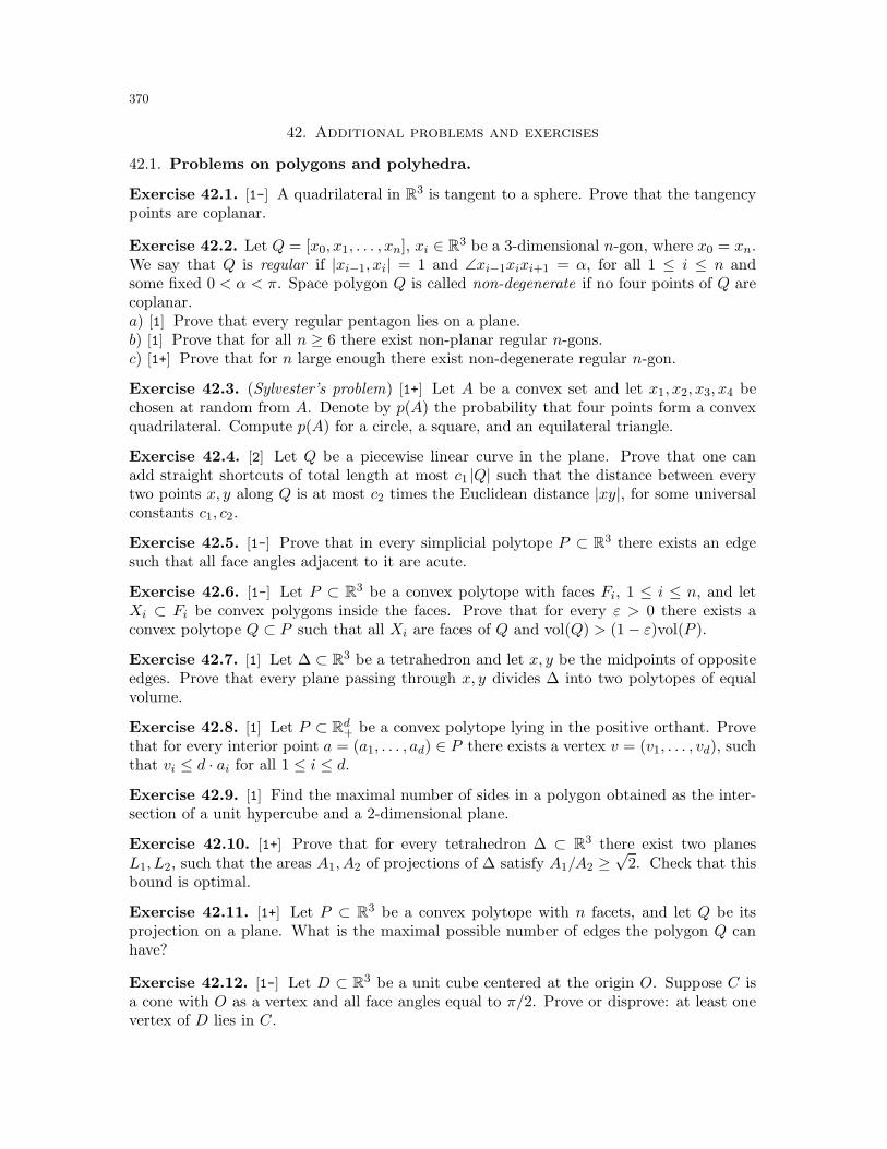
370

42. Additional problems and exercises

42.1. Problems on polygons and polyhedra.

Exercise 42.1. [1-] A quadrilateral in R3 is tangent to a sphere. Prove that the tangencypoints are coplanar.

Exercise 42.2. Let Q = [x0, x1, . . . , xn], xi ∈ R3 be a 3-dimensional n-gon, where x0 = xn.We say that Q is regular if |xi−1, xi| = 1 and ∠xi−1xixi+1 = α, for all 1 ≤ i ≤ n andsome fixed 0 < α < π. Space polygon Q is called non-degenerate if no four points of Q arecoplanar.a) [1] Prove that every regular pentagon lies on a plane.b) [1] Prove that for all n ≥ 6 there exist non-planar regular n-gons.c) [1+] Prove that for n large enough there exist non-degenerate regular n-gon.

Exercise 42.3. (Sylvester’s problem) [1+] Let A be a convex set and let x1, x2, x3, x4 bechosen at random from A. Denote by p(A) the probability that four points form a convexquadrilateral. Compute p(A) for a circle, a square, and an equilateral triangle.

Exercise 42.4. [2] Let Q be a piecewise linear curve in the plane. Prove that one canadd straight shortcuts of total length at most c1 |Q| such that the distance between everytwo points x, y along Q is at most c2 times the Euclidean distance |xy|, for some universalconstants c1, c2.

Exercise 42.5. [1-] Prove that in every simplicial polytope P ⊂ R3 there exists an edgesuch that all face angles adjacent to it are acute.

Exercise 42.6. [1-] Let P ⊂ R3 be a convex polytope with faces Fi, 1 ≤ i ≤ n, and letXi ⊂ Fi be convex polygons inside the faces. Prove that for every ε > 0 there exists aconvex polytope Q ⊂ P such that all Xi are faces of Q and vol(Q) > (1− ε)vol(P ).

Exercise 42.7. [1] Let ∆ ⊂ R3 be a tetrahedron and let x, y be the midpoints of oppositeedges. Prove that every plane passing through x, y divides ∆ into two polytopes of equalvolume.

Exercise 42.8. [1] Let P ⊂ Rd+ be a convex polytope lying in the positive orthant. Provethat for every interior point a = (a1, . . . , ad) ∈ P there exists a vertex v = (v1, . . . , vd), suchthat vi ≤ d · ai for all 1 ≤ i ≤ d.

Exercise 42.9. [1] Find the maximal number of sides in a polygon obtained as the inter-section of a unit hypercube and a 2-dimensional plane.

Exercise 42.10. [1+] Prove that for every tetrahedron ∆ ⊂ R3 there exist two planesL1, L2, such that the areas A1, A2 of projections of ∆ satisfy A1/A2 ≥

√2. Check that this

bound is optimal.

Exercise 42.11. [1+] Let P ⊂ R3 be a convex polytope with n facets, and let Q be itsprojection on a plane. What is the maximal possible number of edges the polygon Q canhave?

Exercise 42.12. [1-] Let D ⊂ R3 be a unit cube centered at the origin O. Suppose C isa cone with O as a vertex and all face angles equal to π/2. Prove or disprove: at least onevertex of D lies in C.

371

Exercise 42.13. a) [2] Suppose P ⊂ R3 is a convex body, such that all projections of Pare convex polygons. Prove that P is a convex polytope.b) [2-] Suppose further, that all projections are polygons with at most n sides. Then P has

nO(n) facets.c) [1] Give an explicit construction of polytopes P with eΩ(n) facets.

Exercise 42.14. a) [2] Suppose P ⊂ R3 is a convex body, such that all projections of Pare convex polygons. Prove that P is a convex polytope.b) [2-] Suppose further, that all projections are polygons with at most n sides. Then P has

nO(n) facets.

Exercise 42.15. a) [1] Let P ⊂ R3 be a convex body with countably many extremalpoints. Prove or disprove: the set of extremal points is closed, i.e., the limit of everyconverging sequence of extremal points is also extremal.b) [2] Let P ⊂ R3 be a convex body such that every projection of P on a plane is a convexpolygon. Prove that P is a convex polytope.

Exercise 42.16. (Pohlke’s theorem) [1+] Prove that every convex quadrilateral Q ⊂ R2 isan oblique projection of a regular tetrahedron.

Exercise 42.17. Let Q be a 3-dimensional unit cube.a) [1] Denote by X a projection of Q onto a plane. Prove that 1 ≤ area(X) ≤

√3.

b) [1+] Denote by X the projection of Q onto a plane H, and by ℓ the length of a projectionof Q onto a line orthogonal to H. Prove that ℓ = area(X).c) [1+] Denote by Y a cross section of Q, i.e., the intersection of Q with a plane. Provethat 1 ≤ area(Y ) ≤

√2.

Exercise 42.18. a) [1] Let P ⊂ R3 be a convex polytope, and let ∆ be a tetrahedron withvertices at vertices of P of largest volume. Prove that for every plane H, an orthogonalprojection of ∆ onto H has area at least 1/9 of the area of the projection of P onto H.b) [1+] Improve the above bound to 1/7.

Exercise 42.19. Let P,P ′ ⊂ R3 be two convex polytopes. We say that P passes through P ′

if there exist projections Q and Q′ (of P and P ′) such that Q fits inside Q′. When P = P ′

we say that P passes through itself.98

a) [1] Prove that every tetrahedron passes through itself.b) [1-] Prove that the cube passes through itself.c) [1] Prove that the regular octahedron passes through itself.d) [∗] Prove or disprove: every convex polytope passes through itself.

Exercise 42.20. (Shadows of polytopes) a) [2] Let X ⊂ L be a polygon in the planeL ⊂ R3. Suppose Y ⊂ H is an orthogonal projection of X onto another plane H. Provethat there exists a rigid motion ρ such that ρ(Y ) ⊂ X. In other words, the shadow of anypolygon is smaller than the polygon itself.b) [1-] Show that part a) does not generalize to 3-dimensional convex polytopes in a hy-perplane in R4.c) [1+] Prove that when d ≥ 3 no d-dimensional polytope P can cover all its shadows. Forexample, when d = 4, every convex polytope satisfies b).

98The idea is that in a solid Q one can make a hole so that P can pass through that hole.

372

Exercise 42.21. a) [1-] Let Cd ⊂ Rd be a unit cube, d ≥ 3. Prove that there exists ahyperplane which intersects every facet of Cd.b) [1+] Prove that for every convex polytope P ⊂ R2 and two vertices v,w of P there existsa plane L containing v,w, and such that at least three faces of P are not intersected by L.c) [1+] Prove that for every simplicial convex polytope P ⊂ R3 and two vertices v,w of Pthere exists a hyperplane H containing v,w, and such that at least three facets of P arenot intersected by H.d) [2-] Find a polytope P ⊂ R4 and two vertices v,w, such that every hyperplane Hcontaining v and w intersects all but at most two facets.

Exercise 42.22. [1+] Let P ⊂ R4 be a product of two triangles:

P = (x1, x2, y1, y2) | (x1, x2) ∈ ∆1, (y1, y2) ∈ ∆2.Prove that there are no 9-gon projections of P on a 2-dimensional plane.

Exercise 42.23. [2-] Let P ⊂ R3 be a convex polytope with the property that for everyface F of P there is a parallel face F ′ and a parallel plane L, such that L contains all verticesof P that are not in F or F ′. Prove that K has at most 14 faces. Show that this bound istight.

Exercise 42.24. [1+] Find a polyhedral embedding of a torus which has 7 (non-convex)faces, such that every two faces have a common edge.

Exercise 42.25. [1] Find a polyhedral embedding of a torus which has 7 vertices, 14 tri-angular faces, and such that every two vertices are connected by an edge.

42.2. Volume, area and length problems.

Exercise 42.26. [1-] Let ∆ ⊂ R3 be a tetrahedron. Prove that ∆ has a vertex v, suchthat the lengths of three edges of ∆ adjacent to v satisfy the triangle inequality.

Exercise 42.27. [1] For a tetrahedron ∆ ⊂ R3, denote by h(∆) the minimal height in ∆,and by w(∆) the minimal distance between the opposite edges in ∆. Prove that 2

3 h(∆) ≤w(∆) ≤ h(∆).

Exercise 42.28. (Sarron’s formula) [1] Let X = [x1x2 . . . xn] ⊂ R2 be a simple polygonand let α1, . . . , αn be the angles defined as in Figure 42.1. Denote by ℓi = |xixi+1| the edgelengths of X. Prove:

area(X) =1

2

∑

i<j

ℓiℓj sin(αj − αi) .

Exercise 42.29. [1] Suppose points x1, . . . , xn lie on a unit sphere S2. Prove that∑

1≤i<j≤n|xixj |2 ≤ n2 .

Exercise 42.30. (Law of sines in S2) [1] Let (ABC) ⊂ S2 be a triangle on a unit spherewith edge lengths |BC|S2 = a, |AC|S2 = b, and |AB|S2 = c. Suppose also α = ∢A, β = ∢Band γ = ∢C be the spherical angles in the triangle. Then

sin(a)

sin(α)=

sin(b)

sin(β)=

sin(c)

sin(γ).

373

x1

x2

x3

αn

α1

α2

α3

xn

Figure 42.1. Polygon X = [x1x2 . . . xn] and angles αi in Sarron’s formula.

Exercise 42.31. (Law of sines in R3) [1-] Let a =−→OA, b =

−−→OB and c =

−−→OC be three

non-collinear vectors in R3. Denote by K the cone spanned by these vectors at the origin O.Define the 3-dimensional sine function as

3sin(O,ABC) =[a,b, c]

[a,b] · [a, c] · [b, c],

where [a,b, c] is the volume of a parallelepiped spanned by the vectors; similarly, [a,b] isthe area of a parallelogram spanned by a,b. Consider a tetrahedron (OABC) ⊂ R3. Provethe following law of sines:

area(ABC)3sin(O,ABC)

=area(ABO)

3sin(C,ABO)=

area(ACO)3sin(B,OAC)

=area(BCO)

3sin(A,OBC).

Exercise 42.32. (Polar sine in R3) [1] Let a,b and c be three non-collinear vectors in R3.Define the polar sine function as

psin(a,b, c) =[a,b, c]

‖a‖ · ‖b‖ · ‖c‖ .

For every nonzero vector u in R3, prove the following inequality:

psin(a,b, c) ≤ psin(u ,b, c) + psin(a,u , c) + psin(a,b,u) .

Exercise 42.33. (The law of cosines in R3) [1+] Let P ⊂ R3 be a convex polyhedron withn+ 1 faces F,G1, . . . , Gn. Denote B = area(F ), and Ai = area(Gi), 1 ≤ i ≤ n. Finally, letαij be an angle between between planes spanned by Gi and Gj . Prove that

B2 =

n∑

i=1

A2i −

∑

i6=jAiAj cosαij .

Generalize the result to non-convex polyhedra and to higher dimensions.

Exercise 42.34. [1-] Let x1, x2, x3 ∈ S2 be points on a unit sphere in R3 centered at theorigin O, and let ∆ = (O,x1, x2, x3) be the simplex spanned by these points. Denote by αijthe angles between (O,xi) and (O,xj). Prove that

vol2(∆) =1

36det

1 cosα12 cosα13

cosα12 1 cosα23

cosα13 cosα23 1

.

374

Exercise 42.35. [1] Fix a vertex v of a given tetrahedron ∆. Let a, b, c be the lengths ofedges adjacent to v, and let α, β, γ be the face angles between these edges. Prove that

vol(∆) =abc

3

√ρ(ρ− α)(ρ− β)(ρ− γ) , where ρ =

α+ β + γ

2.

Exercise 42.36. (Kahan’s formula) [1+] Let ∆ = (x1x2x3x4) be a tetrahedron with edgelengths

|x1x2| = a, |x1x3| = b, |x2x3| = c,

|x3x4| = p, |x2x4| = q , |x1x4| = r .

Define

u = (p+ q − c)(p + q + c), v = (p+ r − b)(p + r + b), w = (q + r − a)(q + r + a),

s = (p − q + c)(q − p+ c), t = (p− r + b)(r − p+ b), z = (q − r + a)(r − q + a),

and α =√uvz , β =

√uwt, γ =

√vws, λ =

√stz .

Prove that

vol(∆) =1

192pqr

√(α+ β + γ − λ)(α+ β + λ− γ)(α+ γ + λ− β)(β + γ + λ− α) .

Exercise 42.37. [1] For every six points x1, x2, x3, y1, y2, y3 ∈ R3 define the Cayley–Mengerbideterminant CM(·) as follows:

CM(x1, x2, x3 | y1, y2, y3) = det

0 1 1 11 |x1y1|2 |x1y2|2 |x1y3|21 |x2y1|2 |x2y2|2 |x2y3|21 |x3y1|2 |x3y2|2 |x3y3|2

.

Prove that the dihedral angle ϕ between the planes X = (x1x2x3) and Y = (y1y2y3) satisfies:

cos2 ϕ =CM2(x1, x2, x3 |y1, y2, y3)

CM(x1, x2, x3) · CM(x1, x2, x3).

Exercise 42.38. Let P ⊂ R2 be a convex polygon containing the origin O in its relativeinterior. Denote by fP (r) = area(P ∩ Br), where Br is the circle centered at O of radiusr > 0.a) [1] Suppose fT = fT ′ for two triangles T, T ′ ⊂ R2. Prove that T ≃ T ′.b) [1-] Prove or disprove: if fP = fP ′, then P ≃ P ′.c) [1+] What happens in higher dimensions?

Exercise 42.39. (Euler’s inequality) a) [1-] Let R and r be the circumradius and theinradius of a triangle. Prove that R ≥ 2r.b) [1] Let R and r be the radii of circumscribed and inscribed sphere for a simplex ∆ ⊂ Rd.Prove that R ≥ dr.c) [1+] Show that the volume of a simplex inscribed into a unit sphere in Rd, is maximalfor a regular simplex.d) [1+] Show that the volume of a simplex circumscribed into a unit sphere in Rd, is minimalfor a regular simplex.e) [1-] Deduce part b) from c) and d).

375

42.3. Miscellaneous problems.

Exercise 42.40. a) [1] Let Q ⊂ R3 be an unbounded convex polyhedron such that everyprojection of Q onto a plane is a cone. Prove that Q is a 3-dimensional cone.b) [1] Same result for Q ⊂ Rd and projections on all 2-dimensional planes.

Exercise 42.41. a) [1-] Let Q and Q′ be two convex polygons in the XY and XZ planes,respectively such that projections of Q and Q′ on the X line are the same. Prove that thereexists a convex polytope P with projections Q and Q′.b) [1] Generalize this to simple (not necessarily convex) polygons.

Exercise 42.42. a) [1-] Prove that every tiling of a d-dimensional cube by smaller cubescontains at least 2d cubes.b) [1] Prove that a 3-dimensional cube cannot be tiled by a finite number of cubes of distinctsize.c) [2-] Prove that a square can be tiled by a finite number of squares of distinct size.

Exercise 42.43. [1+] A trapezoid is called isosceles if its non-parallel sides have equallengths. Prove that every convex polygon has a dissection into isosceles trapezoids.

Exercise 42.44. a) [1] Prove that an equilateral triangle cannot be tiled by a finite numberof equilateral triangles of different sizes.b) [1+] Prove that no convex polygon can be tiled by a finite number of equilateral trianglesof different sizes.c) [2-] Prove that the plane cannot be tiled with distinct equilateral triangles whose sidelength are at least 1.d) [1] Prove that an isosceles right triangle can be tiled by a finite number of isosceles righttriangles of different sizes.e) [1+] Prove that every non-equilateral triangle T can be tiled by a finite number of trianglessimilar to T and of different sizes.f) [2-] Prove that a square can be tiled by a finite number of isosceles right triangles ofdifferent sizes.

Exercise 42.45. Two convex polytopes in R3 are called adjacent if they touch by a face.a) [1-] Find eight pairwise adjacent tetrahedra.b) [1+] Prove that there are no 100 pairwise adjacent tetrahedra.c) [1+] For every n, find a family of n pairwise adjacent convex polytopes.d) [2] For every n, find a family of n pairwise adjacent congruent convex polytopes.

Exercise 42.46. Let Q be a convex polygon in the plane. Points x1, . . . , xn ∈ ∂Q aresaid to fix Q, if for every direction on the plane an infinitesimal translation of Q in thatdirection contains one of the xi in its relative interior.a) [1] Prove that one can always find six points which fix Q.b) [1] Prove that six points is necessary only when Q is a hexagon with parallel edges.

Exercise 42.47. Let P1, P2, . . . ,⊂ Rd be a family of non-intersecting convex bodies. We saythat Pi can be extracted if there exists a continuous vector valued function f : [0,∞)→ Rd

such that ‖f(t)‖ = t and a polytopes P1, . . . , Pi + f(t), . . . , Pn are non-intersecting for allt ≥ 0.a) [1] Prove that for d = 2 and a finite family of non-intersecting convex polygons as above,there is always a polygon Pi which can be extracted.

376

b) [1] Prove that for d = 2 and a finite family of three or more non-intersecting convexbodies, at least three of them can be extracted.c) [1+] Prove that for all d and any finite family of d+1 or more balls in Rd (not necessarilyof the same radius), then at least one can be extracted.d) [1+] For d = 3, construct an infinite family of non-intersecting convex polytopes Pi whichlie between two parallel planes, and such that none can be extracted.e) [2-] For d = 3, construct a finite family of non-intersecting convex polytopes Pi suchthat none can be extracted.f) [2-] For d = 3, construct a finite family of non-intersecting unit cubes, such that nonecan be extracted.g) [∗] Is it always possible, for a given convex polytope P ⊂ R3, to construct a finite familyof polytopes congruent to P such that none can be extracted?h) [2+] We say that a family of polytopes Q1, . . . , Qk ⊂ R3 can be extracted from a familyof polytopes Q′

1, . . . , Q′ℓ ⊂ R3 if for some f : [0,∞) → R3, ‖f(t)‖ = t, and some fixed k,

1 < k ≤ n, polytopes Q1, . . . , Qk, Q′1 + f(t), . . . , Q′

ℓ + f(t) are non-intersecting. A familyof polytopes P = P1, . . . , Pn in R3 can be taken apart with two hands if some subset Aof P can be extracted from PrA. Find a finite family of non-intersecting convex polytopeswhich cannot be taken apart with two hands.

377

Hints, solutions and references to selected exercises

1.2. For b), consider all halfspaces defining P , and suppose all normals are in generalposition.

1.3. By Corollary 1.7, it suffices to check that every three vertices of Q lie inside a circleof radius L/4. For obtuse triangles the claim is trivial, and for acute triangles the claimfor the circumradius can be checked directly. For a generalization and another proof seesection 24.1.

1.4. This problem is given by V. Proizvolov in [Kvant], M1665 (1993, no. 3).

1.5. Start with the largest area triangle ∆ with vertices at zi.

1.8 and 1.9. See [BajB].

1.10. See [BolS, §19].

1.11. a), b) and c) These are special cases of results by Molnar and Baker. See [Bak] forthe references.

1.12. a) From part a) of the previous exercise and the logic as in the proof of Corollary 1.7,it suffices to check that no four spherical circles of radius r can cover S2. This follows fromthe area argument when r < π/3.For b), when r = π/2 − ε, the claim is not true; vertices of a regular tetrahedron give acounterexample. The bound r < 2 arcsin 1√

3given by this example is optimal.

1.13. See [Leic, §1.7] and [DGK, §5].

1.14. Part b) is a discrete version of [Hal1]. Similarly, parts c) and d) are discrete versionsof special cases of [Hal2].

1.15. See [YagB], Problem 20.

1.16. Part a) is due to Berge (1959) and part b) is due to Breen (1990). We refer to [BarM]for references, details and extensions.

1.17. This is proved in [BolS, §21].

1.19. An ingenious solution of this problem is given by N. B. Vasiliev in [Kvant], M30 (1971,no. 4).

1.20. See [ErdP, §6.4] for references and related results.

1.22. Both results are due to Breen [Bre].

1.23. A short proof is given in [Gug4].

1.24. This is due to Dvoretzky [Dvo] (see also [BZ2, §6]).

1.25. Part a) is due to Schreier (1933) and the generalization to higher dimension is due toAumann (1936). See [BZ2, §5] for further results and references.

1.26. See [Rub].

2.1. Note that in R4 the facets can intersect by a 2-dimensional face which can have differenttriangulations on each side.

2.3. a) Denote by n, ℓ, and m the number of points, line intervals and regions in the plane.Prove by induction that n− ℓ+m = 1 (or use Euler’s formula). We have:

n =∑

i≥2

pi , ℓ =∑

i≥2

ipi, m =∑

j≥3

qj , 2ℓ =∑

j≥3

jqi ,

3 = (3n − ℓ) + (3m− 2ℓ) =∑

i≥2

(3− i)pi +∑

j≥3

(3− j)qi ,

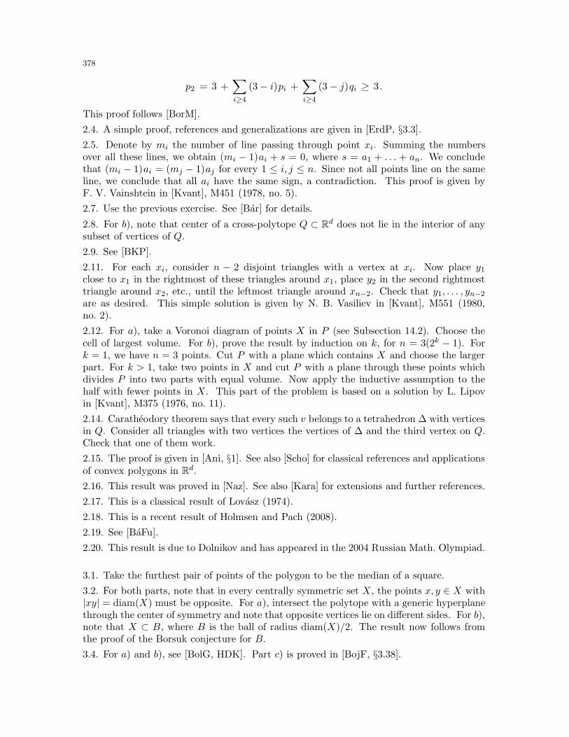
378

p2 = 3 +∑

i≥4

(3− i)pi +∑

i≥4

(3− j)qi ≥ 3.

This proof follows [BorM].

2.4. A simple proof, references and generalizations are given in [ErdP, §3.3].

2.5. Denote by mi the number of line passing through point xi. Summing the numbersover all these lines, we obtain (mi − 1)ai + s = 0, where s = a1 + . . . + an. We concludethat (mi − 1)ai = (mj − 1)aj for every 1 ≤ i, j ≤ n. Since not all points line on the sameline, we conclude that all ai have the same sign, a contradiction. This proof is given byF. V. Vainshtein in [Kvant], M451 (1978, no. 5).

2.7. Use the previous exercise. See [Bar] for details.

2.8. For b), note that center of a cross-polytope Q ⊂ Rd does not lie in the interior of anysubset of vertices of Q.

2.9. See [BKP].

2.11. For each xi, consider n − 2 disjoint triangles with a vertex at xi. Now place y1

close to x1 in the rightmost of these triangles around x1, place y2 in the second rightmosttriangle around x2, etc., until the leftmost triangle around xn−2. Check that y1, . . . , yn−2

are as desired. This simple solution is given by N. B. Vasiliev in [Kvant], M551 (1980,no. 2).

2.12. For a), take a Voronoi diagram of points X in P (see Subsection 14.2). Choose thecell of largest volume. For b), prove the result by induction on k, for n = 3(2k − 1). Fork = 1, we have n = 3 points. Cut P with a plane which contains X and choose the largerpart. For k > 1, take two points in X and cut P with a plane through these points whichdivides P into two parts with equal volume. Now apply the inductive assumption to thehalf with fewer points in X. This part of the problem is based on a solution by L. Lipovin [Kvant], M375 (1976, no. 11).

2.14. Caratheodory theorem says that every such v belongs to a tetrahedron ∆ with verticesin Q. Consider all triangles with two vertices the vertices of ∆ and the third vertex on Q.Check that one of them work.

2.15. The proof is given in [Ani, §1]. See also [Scho] for classical references and applicationsof convex polygons in Rd.

2.16. This result was proved in [Naz]. See also [Kara] for extensions and further references.

2.17. This is a classical result of Lovasz (1974).

2.18. This is a recent result of Holmsen and Pach (2008).

2.19. See [BaFu].

2.20. This result is due to Dolnikov and has appeared in the 2004 Russian Math. Olympiad.

3.1. Take the furthest pair of points of the polygon to be the median of a square.

3.2. For both parts, note that in every centrally symmetric set X, the points x, y ∈ X with|xy| = diam(X) must be opposite. For a), intersect the polytope with a generic hyperplanethrough the center of symmetry and note that opposite vertices lie on different sides. For b),note that X ⊂ B, where B is the ball of radius diam(X)/2. The result now follows fromthe proof of the Borsuk conjecture for B.

3.4. For a) and b), see [BolG, HDK]. Part c) is proved in [BojF, §3.38].

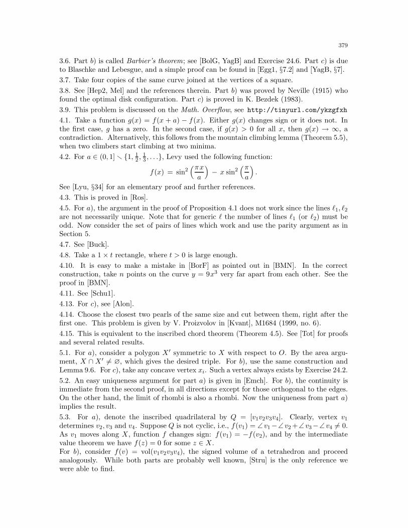
379

3.6. Part b) is called Barbier’s theorem; see [BolG, YagB] and Exercise 24.6. Part c) is dueto Blaschke and Lebesgue, and a simple proof can be found in [Egg1, §7.2] and [YagB, §7].

3.7. Take four copies of the same curve joined at the vertices of a square.

3.8. See [Hep2, Mel] and the references therein. Part b) was proved by Neville (1915) whofound the optimal disk configuration. Part c) is proved in K. Bezdek (1983).

3.9. This problem is discussed on the Math. Overflow, see http://tinyurl.com/ykzgfxh

4.1. Take a function g(x) = f(x + a) − f(x). Either g(x) changes sign or it does not. Inthe first case, g has a zero. In the second case, if g(x) > 0 for all x, then g(x) → ∞, acontradiction. Alternatively, this follows from the mountain climbing lemma (Theorem 5.5),when two climbers start climbing at two minima.

4.2. For a ∈ (0, 1] r 1, 12 ,

13 , . . ., Levy used the following function:

f(x) = sin2(πxa

)− x sin2

(πa

).

See [Lyu, §34] for an elementary proof and further references.

4.3. This is proved in [Ros].

4.5. For a), the argument in the proof of Proposition 4.1 does not work since the lines ℓ1, ℓ2are not necessarily unique. Note that for generic ℓ the number of lines ℓ1 (or ℓ2) must beodd. Now consider the set of pairs of lines which work and use the parity argument as inSection 5.

4.7. See [Buck].

4.8. Take a 1× t rectangle, where t > 0 is large enough.

4.10. It is easy to make a mistake in [BorF] as pointed out in [BMN]. In the correctconstruction, take n points on the curve y = 9x3 very far apart from each other. See theproof in [BMN].

4.11. See [Schu1].

4.13. For c), see [Alon].

4.14. Choose the closest two pearls of the same size and cut between them, right after thefirst one. This problem is given by V. Proizvolov in [Kvant], M1684 (1999, no. 6).

4.15. This is equivalent to the inscribed chord theorem (Theorem 4.5). See [Tot] for proofsand several related results.

5.1. For a), consider a polygon X ′ symmetric to X with respect to O. By the area argu-ment, X ∩X ′ 6= ∅, which gives the desired triple. For b), use the same construction andLemma 9.6. For c), take any concave vertex xi. Such a vertex always exists by Exercise 24.2.

5.2. An easy uniqueness argument for part a) is given in [Emch]. For b), the continuity isimmediate from the second proof, in all directions except for those orthogonal to the edges.On the other hand, the limit of rhombi is also a rhombi. Now the uniqueness from part a)implies the result.

5.3. For a), denote the inscribed quadrilateral by Q = [v1v2v3v4]. Clearly, vertex v1determines v2, v3 and v4. Suppose Q is not cyclic, i.e., f(v1) = ∠ v1−∠ v2 +∠ v3−∠ v4 6= 0.As v1 moves along X, function f changes sign: f(v1) = −f(v2), and by the intermediatevalue theorem we have f(z) = 0 for some z ∈ X.For b), consider f(v) = vol(v1v2v3v4), the signed volume of a tetrahedron and proceedanalogously. While both parts are probably well known, [Stru] is the only reference wewere able to find.

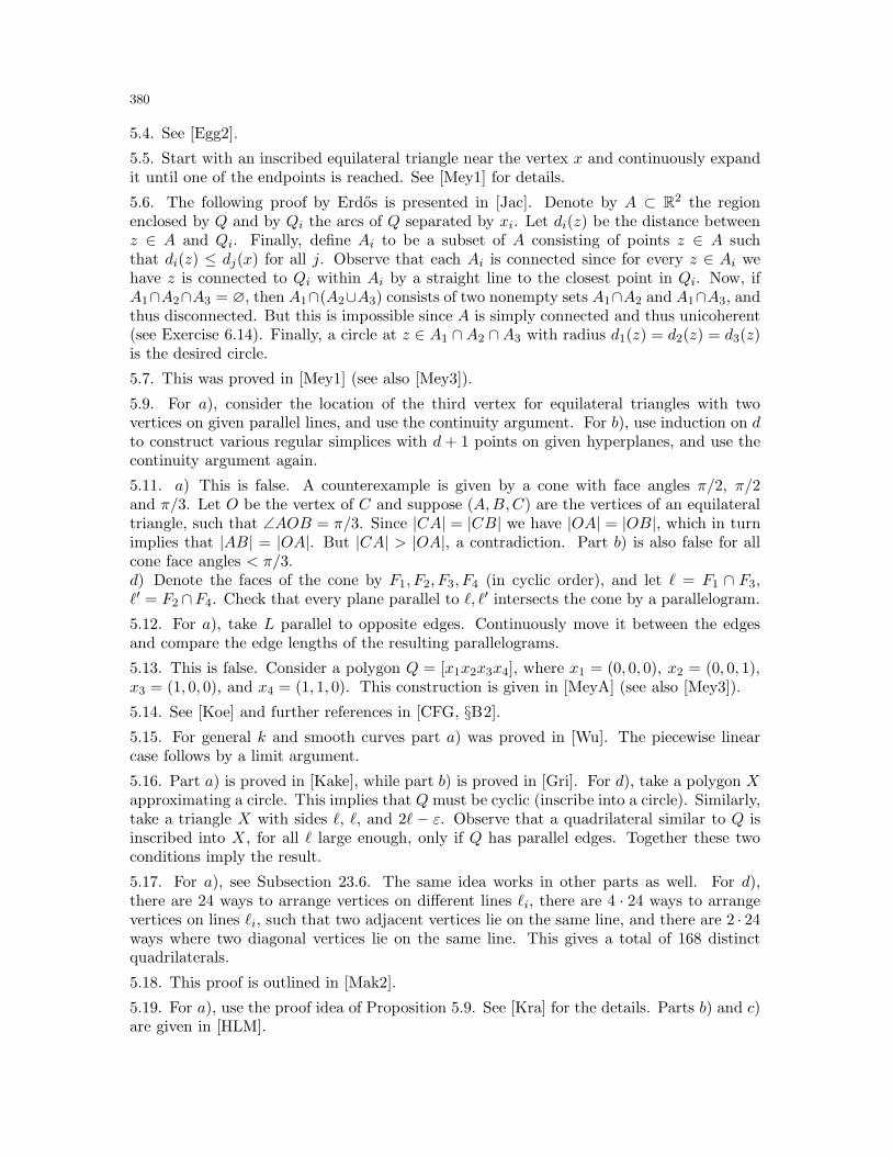
380

5.4. See [Egg2].

5.5. Start with an inscribed equilateral triangle near the vertex x and continuously expandit until one of the endpoints is reached. See [Mey1] for details.

5.6. The following proof by Erdos is presented in [Jac]. Denote by A ⊂ R2 the regionenclosed by Q and by Qi the arcs of Q separated by xi. Let di(z) be the distance betweenz ∈ A and Qi. Finally, define Ai to be a subset of A consisting of points z ∈ A suchthat di(z) ≤ dj(x) for all j. Observe that each Ai is connected since for every z ∈ Ai wehave z is connected to Qi within Ai by a straight line to the closest point in Qi. Now, ifA1∩A2∩A3 = ∅, then A1∩(A2∪A3) consists of two nonempty sets A1∩A2 and A1∩A3, andthus disconnected. But this is impossible since A is simply connected and thus unicoherent(see Exercise 6.14). Finally, a circle at z ∈ A1 ∩A2 ∩A3 with radius d1(z) = d2(z) = d3(z)is the desired circle.

5.7. This was proved in [Mey1] (see also [Mey3]).

5.9. For a), consider the location of the third vertex for equilateral triangles with twovertices on given parallel lines, and use the continuity argument. For b), use induction on dto construct various regular simplices with d+ 1 points on given hyperplanes, and use thecontinuity argument again.

5.11. a) This is false. A counterexample is given by a cone with face angles π/2, π/2and π/3. Let O be the vertex of C and suppose (A,B,C) are the vertices of an equilateraltriangle, such that ∠AOB = π/3. Since |CA| = |CB| we have |OA| = |OB|, which in turnimplies that |AB| = |OA|. But |CA| > |OA|, a contradiction. Part b) is also false for allcone face angles < π/3.d) Denote the faces of the cone by F1, F2, F3, F4 (in cyclic order), and let ℓ = F1 ∩ F3,ℓ′ = F2 ∩F4. Check that every plane parallel to ℓ, ℓ′ intersects the cone by a parallelogram.

5.12. For a), take L parallel to opposite edges. Continuously move it between the edgesand compare the edge lengths of the resulting parallelograms.

5.13. This is false. Consider a polygon Q = [x1x2x3x4], where x1 = (0, 0, 0), x2 = (0, 0, 1),x3 = (1, 0, 0), and x4 = (1, 1, 0). This construction is given in [MeyA] (see also [Mey3]).

5.14. See [Koe] and further references in [CFG, §B2].

5.15. For general k and smooth curves part a) was proved in [Wu]. The piecewise linearcase follows by a limit argument.

5.16. Part a) is proved in [Kake], while part b) is proved in [Gri]. For d), take a polygon Xapproximating a circle. This implies that Q must be cyclic (inscribe into a circle). Similarly,take a triangle X with sides ℓ, ℓ, and 2ℓ − ε. Observe that a quadrilateral similar to Q isinscribed into X, for all ℓ large enough, only if Q has parallel edges. Together these twoconditions imply the result.

5.17. For a), see Subsection 23.6. The same idea works in other parts as well. For d),there are 24 ways to arrange vertices on different lines ℓi, there are 4 · 24 ways to arrangevertices on lines ℓi, such that two adjacent vertices lie on the same line, and there are 2 · 24ways where two diagonal vertices lie on the same line. This gives a total of 168 distinctquadrilaterals.

5.18. This proof is outlined in [Mak2].

5.19. For a), use the proof idea of Proposition 5.9. See [Kra] for the details. Parts b) and c)are given in [HLM].

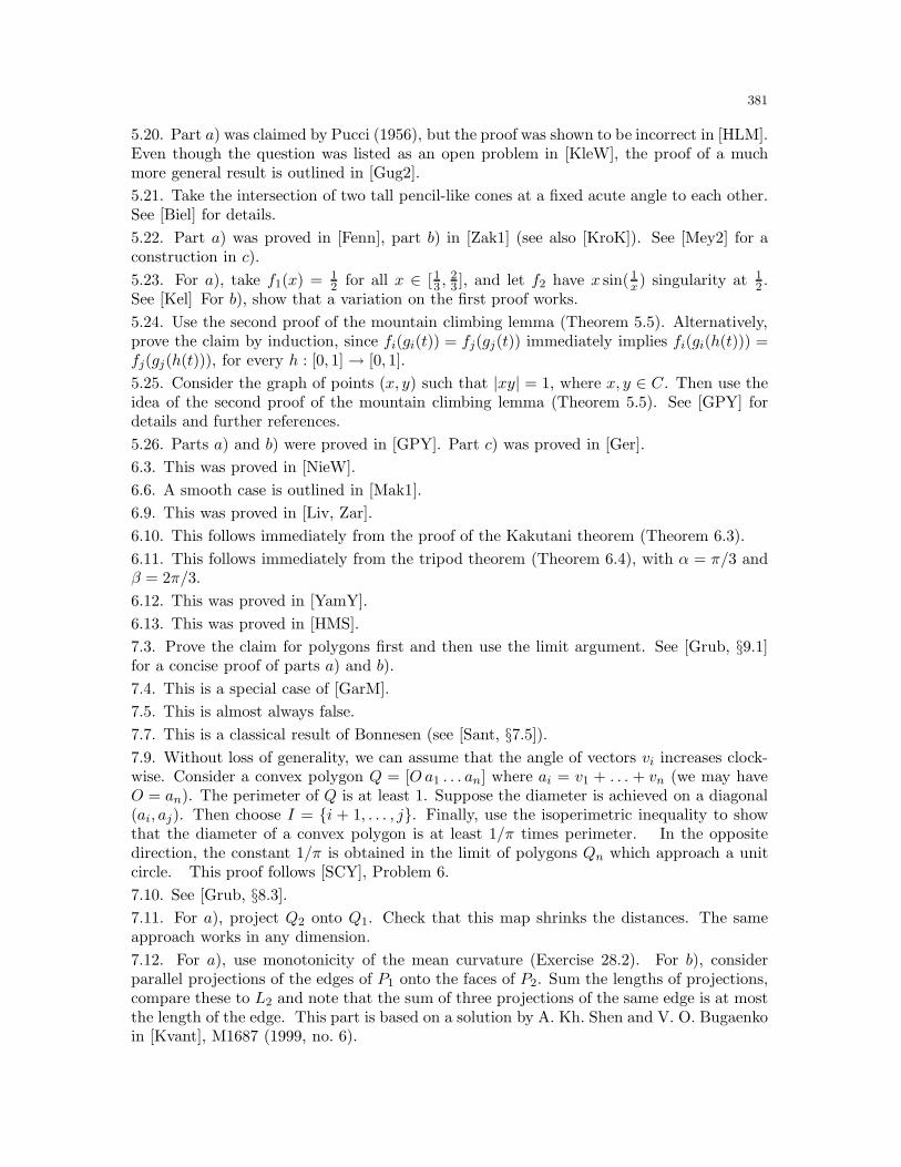
381

5.20. Part a) was claimed by Pucci (1956), but the proof was shown to be incorrect in [HLM].Even though the question was listed as an open problem in [KleW], the proof of a muchmore general result is outlined in [Gug2].

5.21. Take the intersection of two tall pencil-like cones at a fixed acute angle to each other.See [Biel] for details.

5.22. Part a) was proved in [Fenn], part b) in [Zak1] (see also [KroK]). See [Mey2] for aconstruction in c).

5.23. For a), take f1(x) = 12 for all x ∈ [13 ,

23 ], and let f2 have x sin( 1

x) singularity at 12 .

See [Kel] For b), show that a variation on the first proof works.

5.24. Use the second proof of the mountain climbing lemma (Theorem 5.5). Alternatively,prove the claim by induction, since fi(gi(t)) = fj(gj(t)) immediately implies fi(gi(h(t))) =fj(gj(h(t))), for every h : [0, 1]→ [0, 1].

5.25. Consider the graph of points (x, y) such that |xy| = 1, where x, y ∈ C. Then use theidea of the second proof of the mountain climbing lemma (Theorem 5.5). See [GPY] fordetails and further references.

5.26. Parts a) and b) were proved in [GPY]. Part c) was proved in [Ger].

6.3. This was proved in [NieW].

6.6. A smooth case is outlined in [Mak1].

6.9. This was proved in [Liv, Zar].

6.10. This follows immediately from the proof of the Kakutani theorem (Theorem 6.3).

6.11. This follows immediately from the tripod theorem (Theorem 6.4), with α = π/3 andβ = 2π/3.

6.12. This was proved in [YamY].

6.13. This was proved in [HMS].

7.3. Prove the claim for polygons first and then use the limit argument. See [Grub, §9.1]for a concise proof of parts a) and b).

7.4. This is a special case of [GarM].

7.5. This is almost always false.

7.7. This is a classical result of Bonnesen (see [Sant, §7.5]).

7.9. Without loss of generality, we can assume that the angle of vectors vi increases clock-wise. Consider a convex polygon Q = [O a1 . . . an] where ai = v1 + . . . + vn (we may haveO = an). The perimeter of Q is at least 1. Suppose the diameter is achieved on a diagonal(ai, aj). Then choose I = i + 1, . . . , j. Finally, use the isoperimetric inequality to showthat the diameter of a convex polygon is at least 1/π times perimeter. In the oppositedirection, the constant 1/π is obtained in the limit of polygons Qn which approach a unitcircle. This proof follows [SCY], Problem 6.

7.10. See [Grub, §8.3].

7.11. For a), project Q2 onto Q1. Check that this map shrinks the distances. The sameapproach works in any dimension.

7.12. For a), use monotonicity of the mean curvature (Exercise 28.2). For b), considerparallel projections of the edges of P1 onto the faces of P2. Sum the lengths of projections,compare these to L2 and note that the sum of three projections of the same edge is at mostthe length of the edge. This part is based on a solution by A. Kh. Shen and V. O. Bugaenkoin [Kvant], M1687 (1999, no. 6).

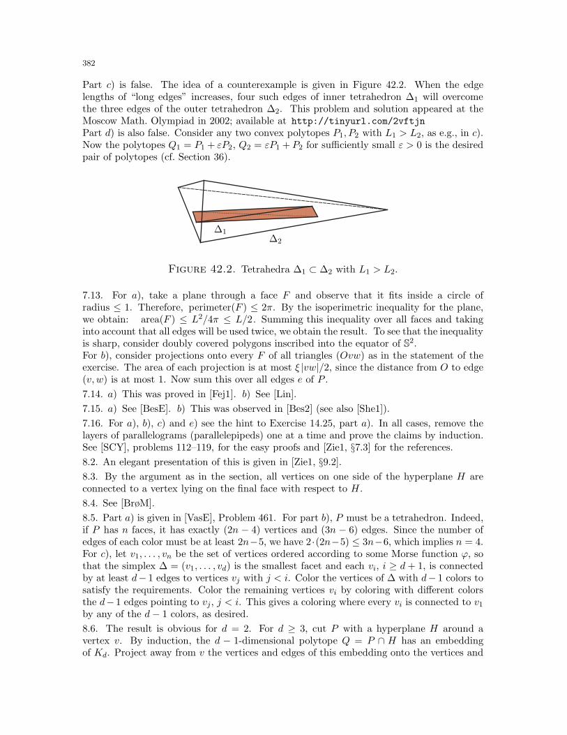
382

Part c) is false. The idea of a counterexample is given in Figure 42.2. When the edgelengths of “long edges” increases, four such edges of inner tetrahedron ∆1 will overcomethe three edges of the outer tetrahedron ∆2. This problem and solution appeared at theMoscow Math. Olympiad in 2002; available at http://tinyurl.com/2vftjn

Part d) is also false. Consider any two convex polytopes P1, P2 with L1 > L2, as e.g., in c).Now the polytopes Q1 = P1 + εP2, Q2 = εP1 + P2 for sufficiently small ε > 0 is the desiredpair of polytopes (cf. Section 36).

∆1∆2

Figure 42.2. Tetrahedra ∆1 ⊂ ∆2 with L1 > L2.

7.13. For a), take a plane through a face F and observe that it fits inside a circle ofradius ≤ 1. Therefore, perimeter(F ) ≤ 2π. By the isoperimetric inequality for the plane,we obtain: area(F ) ≤ L2/4π ≤ L/2. Summing this inequality over all faces and takinginto account that all edges will be used twice, we obtain the result. To see that the inequalityis sharp, consider doubly covered polygons inscribed into the equator of S2.For b), consider projections onto every F of all triangles (Ovw) as in the statement of theexercise. The area of each projection is at most ξ |vw|/2, since the distance from O to edge(v,w) is at most 1. Now sum this over all edges e of P .

7.14. a) This was proved in [Fej1]. b) See [Lin].

7.15. a) See [BesE]. b) This was observed in [Bes2] (see also [She1]).

7.16. For a), b), c) and e) see the hint to Exercise 14.25, part a). In all cases, remove thelayers of parallelograms (parallelepipeds) one at a time and prove the claims by induction.See [SCY], problems 112–119, for the easy proofs and [Zie1, §7.3] for the references.

8.2. An elegant presentation of this is given in [Zie1, §9.2].

8.3. By the argument as in the section, all vertices on one side of the hyperplane H areconnected to a vertex lying on the final face with respect to H.

8.4. See [BrøM].

8.5. Part a) is given in [VasE], Problem 461. For part b), P must be a tetrahedron. Indeed,if P has n faces, it has exactly (2n − 4) vertices and (3n − 6) edges. Since the number ofedges of each color must be at least 2n−5, we have 2·(2n−5) ≤ 3n−6, which implies n = 4.For c), let v1, . . . , vn be the set of vertices ordered according to some Morse function ϕ, sothat the simplex ∆ = (v1, . . . , vd) is the smallest facet and each vi, i ≥ d+ 1, is connectedby at least d− 1 edges to vertices vj with j < i. Color the vertices of ∆ with d− 1 colors tosatisfy the requirements. Color the remaining vertices vi by coloring with different colorsthe d− 1 edges pointing to vj, j < i. This gives a coloring where every vi is connected to v1by any of the d− 1 colors, as desired.

8.6. The result is obvious for d = 2. For d ≥ 3, cut P with a hyperplane H around avertex v. By induction, the d − 1-dimensional polytope Q = P ∩ H has an embeddingof Kd. Project away from v the vertices and edges of this embedding onto the vertices and

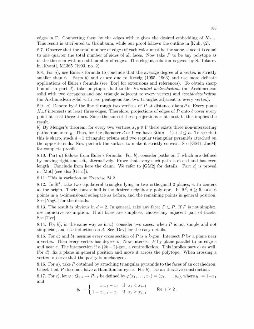
383

edges in Γ. Connecting them by the edges with v gives the desired embedding of Kd+1.This result is attributed to Grunbaum, while our proof follows the outline in [Kuh, §2].

8.7. Observe that the total number of edges of each color must be the same, since it is equalto one quarter the total number of sides of all faces. Now take P to be any polytope asin the theorem with an odd number of edges. This elegant solution is given by S. Tokarevin [Kvant], M1365 (1993, no. 2).

8.8. For a), use Euler’s formula to conclude that the average degree of a vertex is strictlysmaller than 6. Parts b) and c) are due to Kotzig (1955, 1963) and use more delicateapplications of Euler’s formula (see [Bor] for extensions and references). To obtain sharpbounds in part d), take polytopes dual to the truncated dodecahedron (an Archimedeansolid with two decagons and one triangle adjacent to every vertex) and icosidodecahedron(an Archimedean solid with two pentagons and two triangles adjacent to every vertex).

8.9. a) Denote by ℓ the line through two vertices of P at distance diam(P ). Every planeH⊥ℓ intersects at least three edges. Therefore, projections of edges of P onto ℓ cover everypoint at least three times. Since the sum of these projections is at most L, this implies theresult.b) By Menger’s theorem, for every two vertices x, y ∈ Γ there exists three non-intersectingpaths from x to y. Thus, for the diameter d of Γ we have 3th(d − 1) + 2 ≤ n. To see thatthis is sharp, stack d−1 triangular prisms and two regular triangular pyramids attached onthe opposite ends. Now perturb the surface to make it strictly convex. See [GM1, JucM]for complete proofs.

8.10. Part a) follows from Euler’s formula. For b), consider paths on Γ which are definedby moving right and left, alternatively. Prove that every such path is closed and has evenlength. Conclude from here the claim. We refer to [GM2] for details. Part c) is provedin [Mot] (see also [Gru1]).

8.11. This ia variation on Exercise 24.2.

8.12. In R4, take two equilateral triangles lying in two orthogonal 2-planes, with centersat the origin. Their convex hull is the desired neighborly polytope. In Rd, d ≥ 5, take 6points in a 4-dimensional subspace as before, and the remaining points in general position.See [NagC] for the details.

8.13. The result is obvious in d = 2. In general, take any facet F ⊂ P . If F is not simplex,use inductive assumption. If all faces are simplices, choose any adjacent pair of facets.See [Tve].

8.14. For b), in the same way as in a), consider two cases: when P is not simple and notsimplicial, and use induction on d. See [Dev] for the easy details.

8.15. For a) and b), assume every cross section of P is a k-gon. Intersect P by a plane neara vertex. Then every vertex has degree k. Now intersect P by plane parallel to an edge eand near e. The intersection if a (2k− 2)-gon, a contradiction. This implies part c) as well.For d), fix a plane in general position and move it across the polytope. When crossing avertex, observe that the parity is unchanged.

8.16. For a), take P obtained by attaching triangular pyramids to the faces of an octahedron.Check that P does not have a Hamiltonian cycle. For b), use an iterative construction.

8.17. For c), let ϕ : Qn,k → Pn,k be defined by ϕ(x1, . . . , xn) = (y1, . . . , yn), where y1 = 1−x1

and

yi =

xi−1 − xi if xi < xi−1

1 + xi−1 − xi if xi ≥ xi−1for i ≥ 2 .

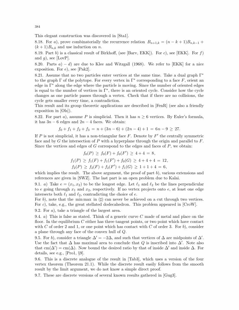
384

This elegant construction was discovered in [Sta1].

8.18. For a), prove combinatorially the recurrence relation Bn+1,k = (n − k + 1)Bn,k−1 +(k + 1)Bn,k and use induction on n.

8.19. Part b) is a classical result of Birkhoff, (see [Barv, EKK]). For c), see [EKK]. For f)and g), see [LovP].

8.20. Parts a) − d) are due to Klee and Witzgall (1968). We refer to [EKK] for a niceexposition. For e), see [Pak2].

8.21. Assume that no two particles enter vertices at the same time. Take a dual graph Γ∗

to the graph Γ of the polytope. For every vertex in Γ∗ corresponding to a face F , orient anedge in Γ∗ along the edge where the particle is moving. Since the number of oriented edgesis equal to the number of vertices in Γ∗, there is an oriented cycle. Consider how the cyclechanges as one particle passes through a vertex. Check that if there are no collisions, thecycle gets smaller every time, a contradiction.This result and its group theoretic applications are described in [FenR] (see also a friendlyexposition in [Ols]).

8.22. For part a), assume P is simplicial. Then it has n ≥ 6 vertices. By Euler’s formula,it has 3n− 6 edges and 2n− 4 faces. We obtain:

f0 + f1 + f2 + f3 = n+ (3n − 6) + (2n − 4) + 1 = 6n − 9 ≥ 27.

If P is not simplicial, it has a non-triangular face F . Denote by F ′ the centrally symmetricface and by G the intersection of P with a hyperplane through the origin and parallel to F .Since the vertices and edges of G correspond to the edges and faces of P , we obtain:

f0(P ) ≥ f0(F ) + f0(F ′) ≥ 4 + 4 = 8,

f1(P ) ≥ f1(F ) + f1(F ′) + f0(G) ≥ 4 + 4 + 4 = 12,

f2(P ) ≥ f2(F ) + f2(F ′) + f1(G) ≥ 1 + 1 + 4 = 6,

which implies the result. The above argument, the proof of part b), various extensions andreferences are given in [SWZ]. The last part is an open problem due to Kalai.

9.1. a) Take e = (x1, x2) to be the longest edge. Let ℓ1 and ℓ2 be the lines perpendicularto e going through x1 and x2, respectively. If no vertex projects onto e, at least one edgeintersects both ℓ1 and ℓ2, contradicting the choice of e.For b), note that the min max in (♯) can never be achieved on a cut through two vertices.For c), take, e.g., the great stellated dodecahedron. This problem appeared in [CroW].

9.2. For a), take a triangle of the largest area.

9.4. a) This is false as stated. Think of a generic curve C made of metal and place on thefloor. In the equilibrium C either has three tangent points, or two point which have contactwith C of order 2 and 1, or one point which has contact with C of order 3. For b), considera plane through any face of the convex hull of Q.

9.5. For b), consider a triangle ∆′ = −2∆, and such that vertices of ∆ are midpoints of ∆′.Use the fact that ∆ has maximal area to conclude that Q is inscribed into ∆′. Note alsothat cm(∆′) = cm(∆). Now bound the desired ratio by that of inside ∆′ and inside ∆. Fordetails, see e.g., [Pro1, §9].

9.6. This is a discrete analogue of the result in [Tab3], which uses a version of the fourvertex theorem (Theorem 21.1). While the discrete result easily follows from the smoothresult by the limit argument, we do not know a simple direct proof.

9.7. These are discrete versions of several known results gathered in [Gug3].

385

9.8. This was proved in [DeoK].

9.10. For parts a) and b) see [CGG, Daw2]. See [Hep1] for part c). Part d) is a delicateresult due to Dawson [Daw2]. The main idea is to apply the Minkowski theorem 36.2 tothe simplices. Part e) is in two followup papers by Dawson and coauthors (1998, 2001).

9.11. Consider a degenerate (flat) parallelepiped as in Figure 42.3. Perturb the dihedralangles to make it non-degenerate (still nearly flat). When placed on one of the non-squarefaces, the center of mass lies outside the face, so the polytope rolls.

Figure 42.3. Parallelepiped which can stand only on two faces.

9.12. For b), start with a construction of a 17-gon using the idea of a heptagon in Figure 9.3,optimizing it in such a way that point O can be taken as close to the center of massas possible. Now use this polygon as a cross-section of the slanted cylinder described inExample 9.9. Make the sides slanted far enough so that the center of mass of the resultingpolyhedron projects onto O. We refer to [CGG] for details.Parts c) and d) were recently obtained in [VD1, VD2]. In the plane, think of the projectionpoints as minima of the distance function from cm(Q). Now apply Lemma 9.6.

9.13. For a), this is called the orthic triangle (see [CoxG, §1.6]). For b), see [Phi].

9.15. This nice observation was communicated by Joe O’Rourke.

9.17. Denote by L = ℓ(∆) the length of the longest triangle ∆ = [x1x2x3] inscribed into C.For every point z ∈ C, denote by Rz the longest triangle inscribed into C with z as a vertex.Clearly, ℓ(Rz) = L when z = x1 and z = x2. Take Rz with the smallest length ℓ(Rz), wherez lies between x1 and x2. Check that this is the desired billiard trajectory. See [Bir, §6.6],[Tab6, §6] and [CroS].

9.18. This is proved in [Weg1].

9.19. A direct proof is given in [Kui]. By analogy with the 2-dimensional case, one canreduce this problem to the number of simple closed geodesics on convex bodies in R4, andconclude that there exist at lest four double normals (see [Alb]). We do not know anelementary proof of this result.

9.21. See [Tab2, §4] and [Tab6, §9], for these and other related results, background andreferences (see also [Tab7]). Parts i) and j) are due to R. E. Schwartz (2007).

10.1. For a), consider a regular pyramid ∆ with a face angle τ on the bottom of sidetriangles. The face angle at the top of side triangle is δ = 1 − 2τ . Now, by the proofabove, we need only to check that α1 + α2 6= 2π, i.e., τ 6= π/3. For example, a standardtetrahedron ∆ corresponding to τ = π/4 gives the desired example (see Figure 10.5).b) Consider a truncated regular pyramid as in Figure 42.5. Let the sums of face angles be2π3 + ǫ for the top vertices, and 2π

3 − ǫ for the bottom three. When ǫ/π /∈ Q there are nosimple closed geodesics.

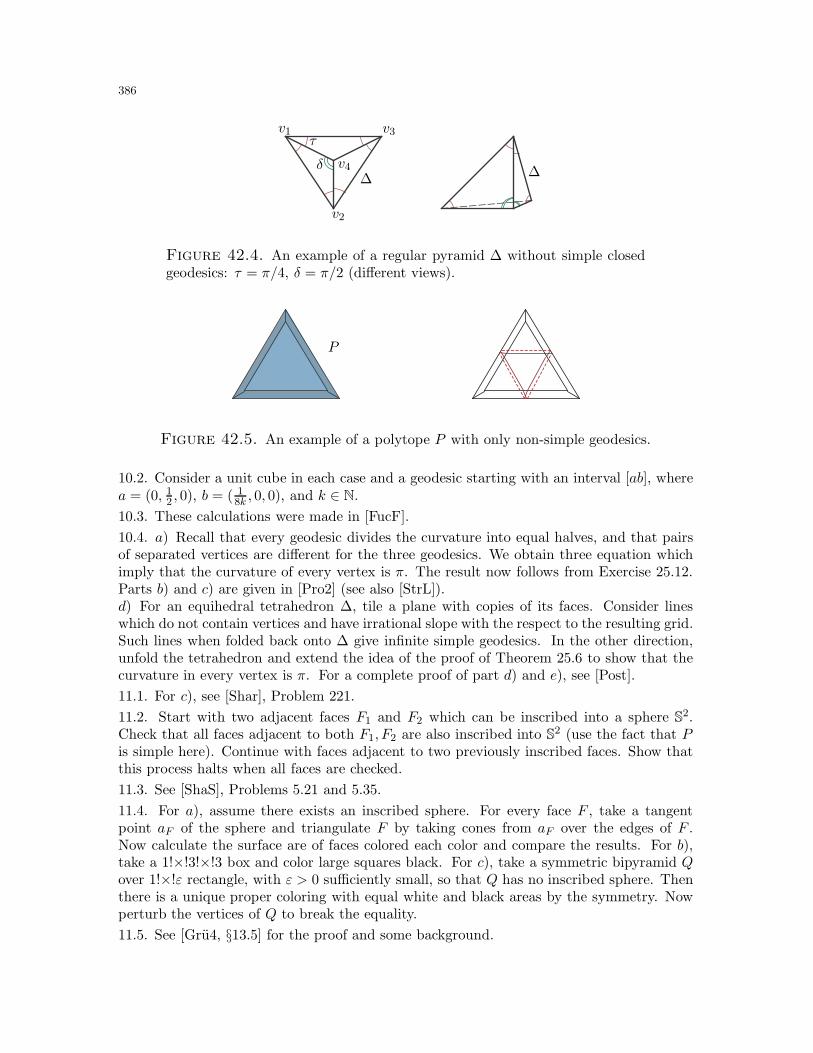
386

τ

δ∆∆

v1

v2

v3

v4

Figure 42.4. An example of a regular pyramid ∆ without simple closedgeodesics: τ = π/4, δ = π/2 (different views).

P

Figure 42.5. An example of a polytope P with only non-simple geodesics.

10.2. Consider a unit cube in each case and a geodesic starting with an interval [ab], wherea = (0, 1

2 , 0), b = ( 18k , 0, 0), and k ∈ N.

10.3. These calculations were made in [FucF].

10.4. a) Recall that every geodesic divides the curvature into equal halves, and that pairsof separated vertices are different for the three geodesics. We obtain three equation whichimply that the curvature of every vertex is π. The result now follows from Exercise 25.12.Parts b) and c) are given in [Pro2] (see also [StrL]).d) For an equihedral tetrahedron ∆, tile a plane with copies of its faces. Consider lineswhich do not contain vertices and have irrational slope with the respect to the resulting grid.Such lines when folded back onto ∆ give infinite simple geodesics. In the other direction,unfold the tetrahedron and extend the idea of the proof of Theorem 25.6 to show that thecurvature in every vertex is π. For a complete proof of part d) and e), see [Post].

11.1. For c), see [Shar], Problem 221.

11.2. Start with two adjacent faces F1 and F2 which can be inscribed into a sphere S2.Check that all faces adjacent to both F1, F2 are also inscribed into S2 (use the fact that Pis simple here). Continue with faces adjacent to two previously inscribed faces. Show thatthis process halts when all faces are checked.

11.3. See [ShaS], Problems 5.21 and 5.35.

11.4. For a), assume there exists an inscribed sphere. For every face F , take a tangentpoint aF of the sphere and triangulate F by taking cones from aF over the edges of F .Now calculate the surface are of faces colored each color and compare the results. For b),take a 1!×!3!×!3 box and color large squares black. For c), take a symmetric bipyramid Qover 1!×!ε rectangle, with ε > 0 sufficiently small, so that Q has no inscribed sphere. Thenthere is a unique proper coloring with equal white and black areas by the symmetry. Nowperturb the vertices of Q to break the equality.

11.5. See [Gru4, §13.5] for the proof and some background.

387

11.6. Part a) is proved in [Bar1]. For b), start with a tetrahedron and construct a pyramidon each face. The resulting polyhedron is dual to the truncated tetrahedron, has 8 verticesand 12 faces. Show that it cannot project onto a regular octahedron. This solution is givenin [Bar2]. Note that this problem is a generalization of Exercise 14.16, corresponding to thecase where P is simplicial and C is a Hamiltonian cycle. Thus part a) of this exercise is ageneralization of c) of Exercise 14.16. Similarly, a counterexample described in the solutionof part b) of Exercise 14.16 also works for part b) in this exercise.

11.7. See [GMS] and [Schu1].

11.8. This is a special case of the main result in [Tho1].

12.2. This is due to Zamfirescu and Gleason (see [Gle] and references therein).

12.3. Both parts are proved in [Schr2] (see also [Var2]).

12.5. Draw two parallel lines and take midpoints of intersections with the parabola. Showthat the line through the midpoints is parallel to the y axis. See [Vard], Problem 23.

12.6. Consider the right triangle with vertices: the center O, the vertex v and the edgemidpoint z of a pentagon. If the pentagon is rational, then cos 3π

10 = |vz|/|vO| =√a for

some a ∈ Q, a contradiction.

12.8. See a construction in [Zie3].

13.4. This result is due to A. Galitzer (see [KM3, §3]).

14.4. See [Epp, ShaH].

14.5. For triangulations of the middle regions, encode them with the 0–1 sequences, whichcorresponds to k− 1 up triangles and k− 1 down triangles. The number of these sequencesis(2k−2k−1

), and two remaining Catalan numbers Ck−2 correspond to triangulations of the top

and bottom k-gons. See [HNU] for the details (see also [DRS, §3.4]).

14.6. This problem was on a 2007 Putnam Mathematical Competition. See a solution here:http://tinyurl.com/2crvn9w

14.7. See [DRS, §3.3].

14.8. For a) see [HNU]. For b) and c), see [Gal+].14.10. For part a), use at most n − 2 moves to transform a given triangulation to atriangulations with all diagonals meeting at the same point. Part b) is proved in [STT]using hyperbolic geometry; a combinatorial proof is given in [Deho]. See also [DRS, San2]for further references.

14.11. Part b) is false (see [BerE]).

14.12. For each of these functionals check that they behave accordingly along increasingflips (essentially, prove the claim for all quadrilaterals). See [BerE] and [Mus2] for more onthis and further references, and [Lam] for g).

14.13. See [Tut, §10] (see also [PouS] for further references, applications and a bijectiveproof).

14.14. For a) and b) use the idea in the example. For c), consider a grid fine enough andadd grid vertices. For parts c)– e) and the references see [BZ4, Mae1, Sar, Zam]. For theprogress towards f), see [ESU]. Part g) was proved in [Kri].

14.15. For a), triangulate the projection and lift it to X. For this and other parts, see [BDE].

14.16. For a), use a binary tree as in Section 8 and lift the triangles up depending how farthey are from the root. Alternatively, take the function ξ as in Example 8.5. For b), take aregular hexagon Q = [x1 . . . x6], triangulations T1 with diagonals (x1, x5), (x2, x4), (x2, x5),

388

and T2 with diagonal (x1, x3), (x1, x4), (x4, x6). See [Dek] for details and further references.See also Exercise 11.6 for a special case of part b) and a generalization of part c).

14.17. For a), take six 1×1×11 bricks and attach each of them in the middle to a unit cube.Now slightly decrease the size of the bricks to make sure they do not intersect.For b), one can use the construction in a). Here is an alternative approach. Solve a 2-dimensional version first and then add two large parallel slabs in R3.

14.18. a) This is one of the oldest results in discrete geometry [Len]. The idea is to find adiagonal inside Q and then use induction. First, project Q onto the x axis and let v be theleftmost vertex. Either the diagonal (u,w) between vertices neighboring v is inside Q, ortriangle (uvw) contains at least one vertex of Q. Then the diagonal (v, z) connecting theleftmost such vertex z with v cannot intersect any edge of Q, and thus lies in the interiorof Q.For parts b) and c), take the Schonhardt’s polyhedron [Scho] (see also an extension in [Ramb]and [Bag]). Simply take a triangular prism and twist the top triangle (see Figure 42.6).We refer to [BerE] and [DRS, §3.5] for the context and further references. Part d) is givenin [Bin].99

For part e), take e.g., six bricks as in part a) of the previous problem and connect them byshort tubes far away from the center.

14.19. See [RupS].

Figure 42.6. Schonhardt’s polyhedron and a non-regular triangulation.

14.20. For a), the standard example is given in Figure 42.6. For b), this is also false, e.g.,for a cuboctahedron (see Figure 16.4). There is also an example with 6 vertices. For therest of the exercise see [San1].

14.21. See [Dil].

14.22. For a), denote by Rt the intersection of a simplex ∆ in the d-cube with a hyperplanex1 = t. Show that vol(Rt) = cti(1− t)d−i, for some c > 0, where i depends on the numberof vertices in ∆ with x1 = 1. Now use the fact that there is a unique linear combination ofpolynomials ti(1− t)d−i equal to a constant. This argument is given in [Glaz]. For b) andfurther references, see [DRS].

14.23. For a), here is a simple ad hoc argument: Draw the edges between centers of squaresinside each domino. Overlap two tilings. Find the innermost circle C. Since both tilingcoincide inside C, use 2-moves to remove this circle. Repeat this procedure until the tilingscoincide.For b), the counterexamples to the first two questions are given in Figure 42.7. For the finalpart, take an n × n square region G in z = 0 level and in the checkerboard fashion add

99An easier example can be found in http://tinyurl.com/radztn.

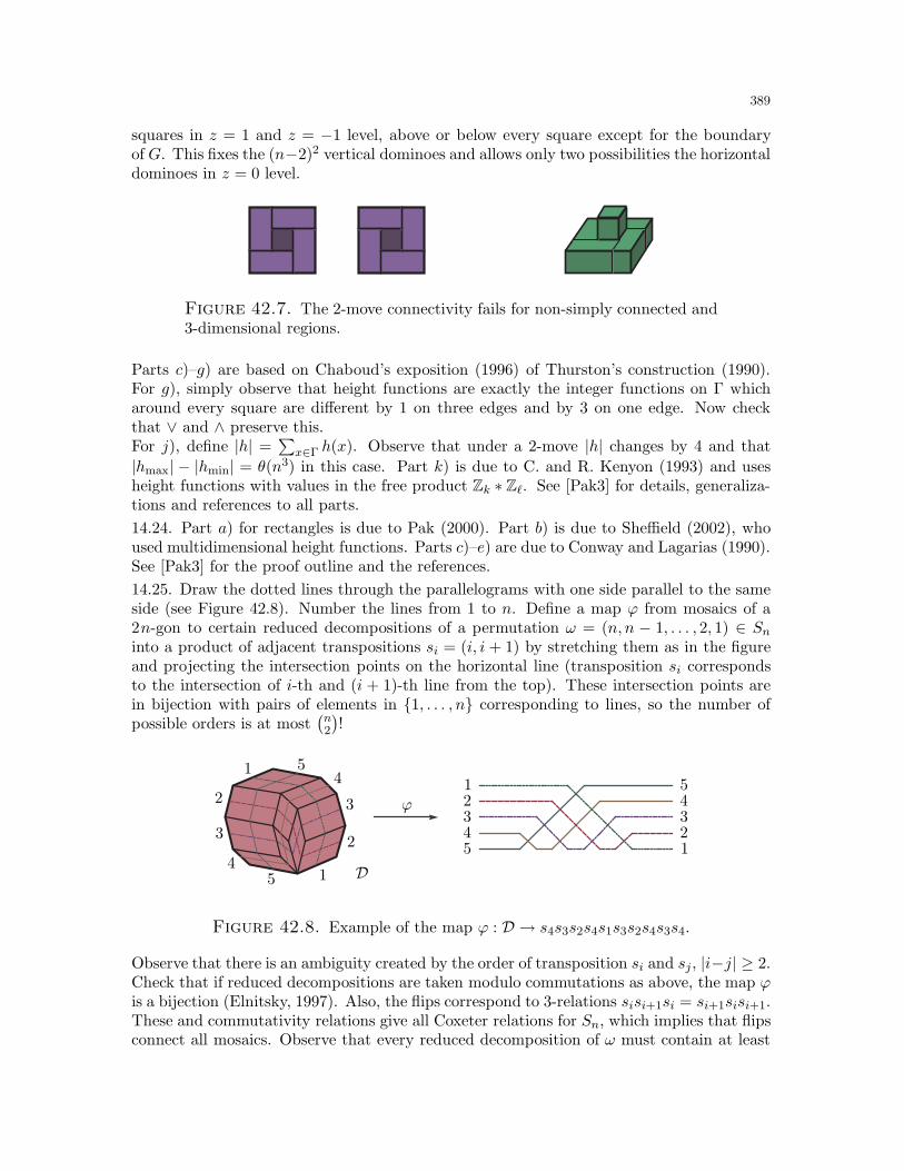
389

squares in z = 1 and z = −1 level, above or below every square except for the boundaryof G. This fixes the (n−2)2 vertical dominoes and allows only two possibilities the horizontaldominoes in z = 0 level.

Figure 42.7. The 2-move connectivity fails for non-simply connected and3-dimensional regions.

Parts c)–g) are based on Chaboud’s exposition (1996) of Thurston’s construction (1990).For g), simply observe that height functions are exactly the integer functions on Γ whicharound every square are different by 1 on three edges and by 3 on one edge. Now checkthat ∨ and ∧ preserve this.For j), define |h| =

∑x∈Γ h(x). Observe that under a 2-move |h| changes by 4 and that

|hmax| − |hmin| = θ(n3) in this case. Part k) is due to C. and R. Kenyon (1993) and usesheight functions with values in the free product Zk ∗ Zℓ. See [Pak3] for details, generaliza-tions and references to all parts.

14.24. Part a) for rectangles is due to Pak (2000). Part b) is due to Sheffield (2002), whoused multidimensional height functions. Parts c)–e) are due to Conway and Lagarias (1990).See [Pak3] for the proof outline and the references.

14.25. Draw the dotted lines through the parallelograms with one side parallel to the sameside (see Figure 42.8). Number the lines from 1 to n. Define a map ϕ from mosaics of a2n-gon to certain reduced decompositions of a permutation ω = (n, n − 1, . . . , 2, 1) ∈ Sninto a product of adjacent transpositions si = (i, i + 1) by stretching them as in the figureand projecting the intersection points on the horizontal line (transposition si correspondsto the intersection of i-th and (i + 1)-th line from the top). These intersection points arein bijection with pairs of elements in 1, . . . , n corresponding to lines, so the number ofpossible orders is at most

(n2

)!

1

1

1

1

2

2

2

233

3

3

4

4

4

4

5

5

5

5

ϕ

D

Figure 42.8. Example of the map ϕ : D → s4s3s2s4s1s3s2s4s3s4.

Observe that there is an ambiguity created by the order of transposition si and sj, |i−j| ≥ 2.Check that if reduced decompositions are taken modulo commutations as above, the map ϕis a bijection (Elnitsky, 1997). Also, the flips correspond to 3-relations sisi+1si = si+1sisi+1.These and commutativity relations give all Coxeter relations for Sn, which implies that flipsconnect all mosaics. Observe that every reduced decomposition of ω must contain at least

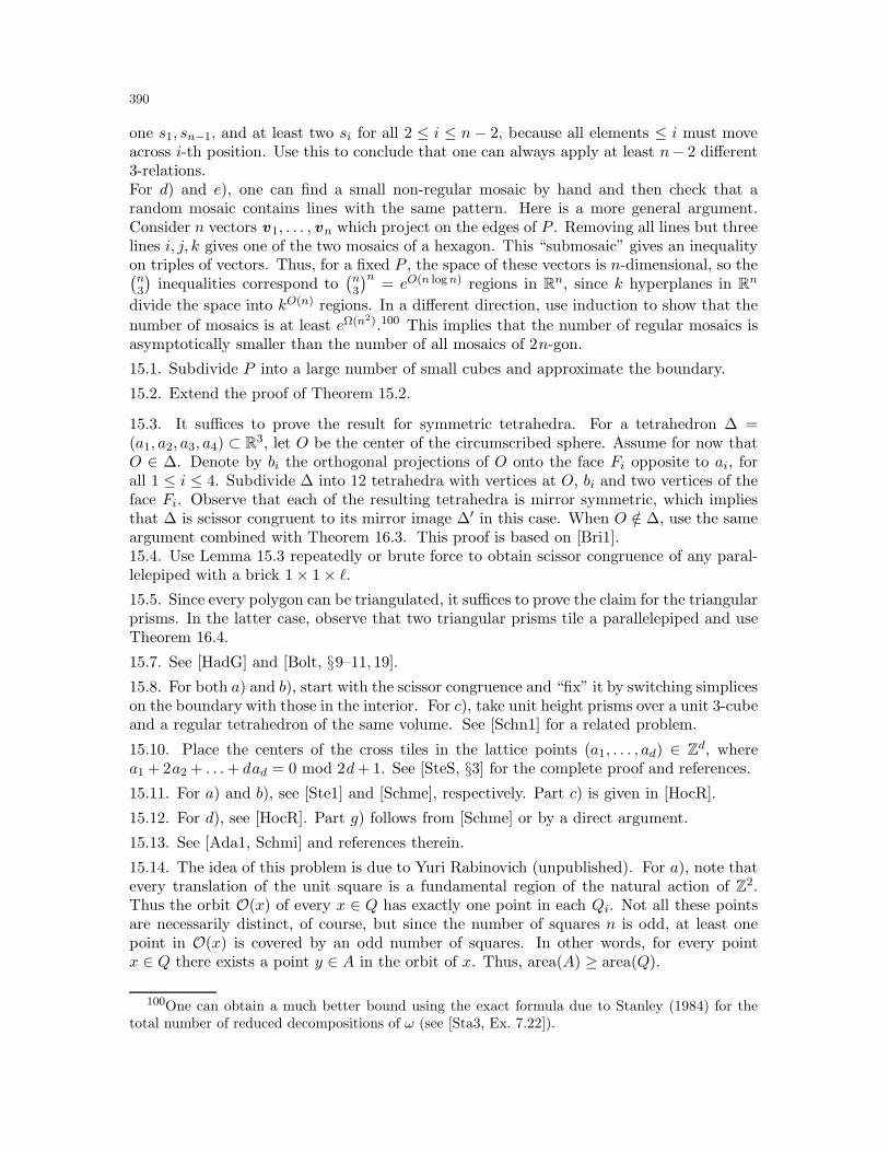
390

one s1, sn−1, and at least two si for all 2 ≤ i ≤ n − 2, because all elements ≤ i must moveacross i-th position. Use this to conclude that one can always apply at least n− 2 different3-relations.For d) and e), one can find a small non-regular mosaic by hand and then check that arandom mosaic contains lines with the same pattern. Here is a more general argument.Consider n vectors v 1, . . . , vn which project on the edges of P . Removing all lines but threelines i, j, k gives one of the two mosaics of a hexagon. This “submosaic” gives an inequalityon triples of vectors. Thus, for a fixed P , the space of these vectors is n-dimensional, so the(n3

)inequalities correspond to

(n3

)n= eO(n logn) regions in Rn, since k hyperplanes in Rn

divide the space into kO(n) regions. In a different direction, use induction to show that the

number of mosaics is at least eΩ(n2).100 This implies that the number of regular mosaics isasymptotically smaller than the number of all mosaics of 2n-gon.

15.1. Subdivide P into a large number of small cubes and approximate the boundary.

15.2. Extend the proof of Theorem 15.2.

15.3. It suffices to prove the result for symmetric tetrahedra. For a tetrahedron ∆ =(a1, a2, a3, a4) ⊂ R3, let O be the center of the circumscribed sphere. Assume for now thatO ∈ ∆. Denote by bi the orthogonal projections of O onto the face Fi opposite to ai, forall 1 ≤ i ≤ 4. Subdivide ∆ into 12 tetrahedra with vertices at O, bi and two vertices of theface Fi. Observe that each of the resulting tetrahedra is mirror symmetric, which impliesthat ∆ is scissor congruent to its mirror image ∆′ in this case. When O /∈ ∆, use the sameargument combined with Theorem 16.3. This proof is based on [Bri1].15.4. Use Lemma 15.3 repeatedly or brute force to obtain scissor congruence of any paral-lelepiped with a brick 1× 1× ℓ.15.5. Since every polygon can be triangulated, it suffices to prove the claim for the triangularprisms. In the latter case, observe that two triangular prisms tile a parallelepiped and useTheorem 16.4.

15.7. See [HadG] and [Bolt, §9–11, 19].

15.8. For both a) and b), start with the scissor congruence and “fix” it by switching simpliceson the boundary with those in the interior. For c), take unit height prisms over a unit 3-cubeand a regular tetrahedron of the same volume. See [Schn1] for a related problem.

15.10. Place the centers of the cross tiles in the lattice points (a1, . . . , ad) ∈ Zd, wherea1 + 2a2 + . . .+ dad = 0 mod 2d+ 1. See [SteS, §3] for the complete proof and references.

15.11. For a) and b), see [Ste1] and [Schme], respectively. Part c) is given in [HocR].

15.12. For d), see [HocR]. Part g) follows from [Schme] or by a direct argument.

15.13. See [Ada1, Schmi] and references therein.

15.14. The idea of this problem is due to Yuri Rabinovich (unpublished). For a), note thatevery translation of the unit square is a fundamental region of the natural action of Z2.Thus the orbit O(x) of every x ∈ Q has exactly one point in each Qi. Not all these pointsare necessarily distinct, of course, but since the number of squares n is odd, at least onepoint in O(x) is covered by an odd number of squares. In other words, for every pointx ∈ Q there exists a point y ∈ A in the orbit of x. Thus, area(A) ≥ area(Q).

100One can obtain a much better bound using the exact formula due to Stanley (1984) for thetotal number of reduced decompositions of ω (see [Sta3, Ex. 7.22]).

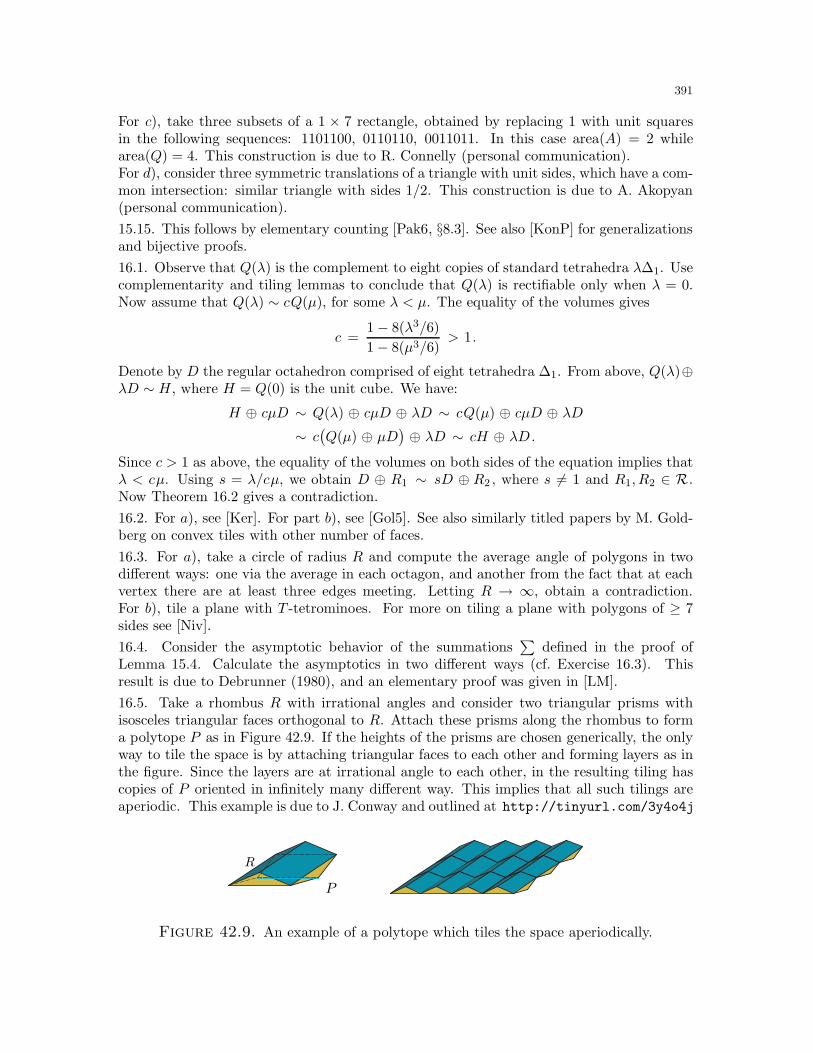
391

For c), take three subsets of a 1 × 7 rectangle, obtained by replacing 1 with unit squaresin the following sequences: 1101100, 0110110, 0011011. In this case area(A) = 2 whilearea(Q) = 4. This construction is due to R. Connelly (personal communication).For d), consider three symmetric translations of a triangle with unit sides, which have a com-mon intersection: similar triangle with sides 1/2. This construction is due to A. Akopyan(personal communication).

15.15. This follows by elementary counting [Pak6, §8.3]. See also [KonP] for generalizationsand bijective proofs.

16.1. Observe that Q(λ) is the complement to eight copies of standard tetrahedra λ∆1. Usecomplementarity and tiling lemmas to conclude that Q(λ) is rectifiable only when λ = 0.Now assume that Q(λ) ∼ cQ(µ), for some λ < µ. The equality of the volumes gives

c =1− 8(λ3/6)

1− 8(µ3/6)> 1.

Denote by D the regular octahedron comprised of eight tetrahedra ∆1. From above, Q(λ)⊕λD ∼ H, where H = Q(0) is the unit cube. We have:

H ⊕ cµD ∼ Q(λ) ⊕ cµD ⊕ λD ∼ cQ(µ) ⊕ cµD ⊕ λD

∼ c(Q(µ) ⊕ µD

)⊕ λD ∼ cH ⊕ λD.

Since c > 1 as above, the equality of the volumes on both sides of the equation implies thatλ < cµ. Using s = λ/cµ, we obtain D ⊕ R1 ∼ sD ⊕ R2 , where s 6= 1 and R1, R2 ∈ R.Now Theorem 16.2 gives a contradiction.

16.2. For a), see [Ker]. For part b), see [Gol5]. See also similarly titled papers by M. Gold-berg on convex tiles with other number of faces.

16.3. For a), take a circle of radius R and compute the average angle of polygons in twodifferent ways: one via the average in each octagon, and another from the fact that at eachvertex there are at least three edges meeting. Letting R → ∞, obtain a contradiction.For b), tile a plane with T -tetrominoes. For more on tiling a plane with polygons of ≥ 7sides see [Niv].

16.4. Consider the asymptotic behavior of the summations∑

defined in the proof ofLemma 15.4. Calculate the asymptotics in two different ways (cf. Exercise 16.3). Thisresult is due to Debrunner (1980), and an elementary proof was given in [LM].

16.5. Take a rhombus R with irrational angles and consider two triangular prisms withisosceles triangular faces orthogonal to R. Attach these prisms along the rhombus to forma polytope P as in Figure 42.9. If the heights of the prisms are chosen generically, the onlyway to tile the space is by attaching triangular faces to each other and forming layers as inthe figure. Since the layers are at irrational angle to each other, in the resulting tiling hascopies of P oriented in infinitely many different way. This implies that all such tilings areaperiodic. This example is due to J. Conway and outlined at http://tinyurl.com/3y4o4j

P

R

Figure 42.9. An example of a polytope which tiles the space aperiodically.

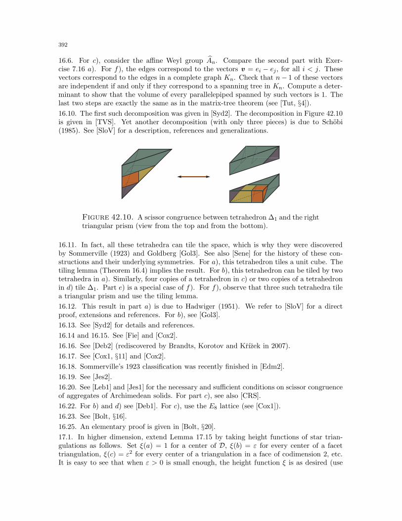
392

16.6. For c), consider the affine Weyl group An. Compare the second part with Exer-cise 7.16 a). For f), the edges correspond to the vectors v = ei − ej , for all i < j. Thesevectors correspond to the edges in a complete graph Kn. Check that n− 1 of these vectorsare independent if and only if they correspond to a spanning tree in Kn. Compute a deter-minant to show that the volume of every parallelepiped spanned by such vectors is 1. Thelast two steps are exactly the same as in the matrix-tree theorem (see [Tut, §4]).

16.10. The first such decomposition was given in [Syd2]. The decomposition in Figure 42.10is given in [TVS]. Yet another decomposition (with only three pieces) is due to Schobi(1985). See [SloV] for a description, references and generalizations.

Figure 42.10. A scissor congruence between tetrahedron ∆1 and the righttriangular prism (view from the top and from the bottom).

16.11. In fact, all these tetrahedra can tile the space, which is why they were discoveredby Sommerville (1923) and Goldberg [Gol3]. See also [Sene] for the history of these con-structions and their underlying symmetries. For a), this tetrahedron tiles a unit cube. Thetiling lemma (Theorem 16.4) implies the result. For b), this tetrahedron can be tiled by twotetrahedra in a). Similarly, four copies of a tetrahedron in c) or two copies of a tetrahedronin d) tile ∆1. Part e) is a special case of f). For f), observe that three such tetrahedra tilea triangular prism and use the tiling lemma.

16.12. This result in part a) is due to Hadwiger (1951). We refer to [SloV] for a directproof, extensions and references. For b), see [Gol3].

16.13. See [Syd2] for details and references.

16.14 and 16.15. See [Fie] and [Cox2].

16.16. See [Deb2] (rediscovered by Brandts, Korotov and Krızek in 2007).

16.17. See [Cox1, §11] and [Cox2].

16.18. Sommerville’s 1923 classification was recently finished in [Edm2].

16.19. See [Jes2].

16.20. See [Leb1] and [Jes1] for the necessary and sufficient conditions on scissor congruenceof aggregates of Archimedean solids. For part c), see also [CRS].

16.22. For b) and d) see [Deb1]. For c), use the E8 lattice (see [Cox1]).

16.23. See [Bolt, §16].

16.25. An elementary proof is given in [Bolt, §20].

17.1. In higher dimension, extend Lemma 17.15 by taking height functions of star trian-gulations as follows. Set ξ(a) = 1 for a center of D, ξ(b) = ε for every center of a facettriangulation, ξ(c) = ε2 for every center of a triangulation in a face of codimension 2, etc.It is easy to see that when ε > 0 is small enough, the height function ξ is as desired (use

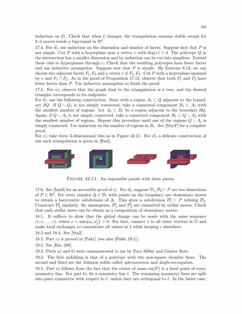
393

induction on d). Check that when ξ changes, the triangulation remains stable except for2–d moves inside a bipyramid in Rd.

17.4. For d), use induction on the dimension and number of facets. Suppose first that P isnot simple. Cut P with a hyperplane near a vertex v with deg(v) > d. The polytope Q inthe intersection has a smaller dimension and by induction can be cut into simplices. Extendthese cuts to hyperplanes through v. Check that the resulting polytopes have fewer facetsand use inductive assumption. Suppose now that P is simple. By Exercise 8.13, we canchoose two adjacent facets F1, F2 and a vertex v /∈ F1, F2. Cut P with a hyperplane spannedby v and F1 ∩ F2. As in the proof of Proposition 17.12, observe that both P1 and P2 havefewer facets than P . Use inductive assumption to finish the proof.

17.5. For a), observe that the graph dual to the triangulation is a tree, and the desiredtriangles corresponds to its endpoints.For b), use the following construction. Start with a region A1 ⊂ Q adjacent to the bound-ary ∂Q. If Q r Q1 is not simply connected, take a connected component B1 ⊂ A1 withthe smallest number of regions. Let A2 ⊂ B1 be a region adjacent to the boundary ∂Q.Again, if Qr A2 is not simply connected, take a connected component B1 ⊂ Qr A2 withthe smallest number of regions. Repeat this procedure until one of the regions Q r Ai issimply connected. Use induction on the number of regions in Bi. See [MucP] for a completeproof.For c), take three 3-dimensional tiles as in Figure 42.11. For d), a delicate construction ofone such triangulation is given in [Rud].

Figure 42.11. An impossible puzzle with three pieces.

17.6. See [IzmS] for an accessible proof of c). For d), suppose D1,D2 ⊢ P are two dissectionsof P ⊂ Rd. For every simplex ∆ ∈ D1 with points on the boundary, use elementary movesto obtain a barycentric subdivision of ∆. This gives a subdivision D′

1 ⊢ P refining D2.Construct D′

2 similarly. By assumption, D′1 and D′

2 are connected by stellar moves. Checkthat each stellar move can be obtain as a composition of elementary moves.

18.1. It suffices to show that the global change can be made with the same sequence(∗, c, . . . , c), where c = minai, a′j > 0. For that, connect 1 to all other vertices in G andmake local exchanges to concentrate all values at 1 while keeping c elsewhere.

18.3 and 18.4. See [Sta2].

18.5. Part c) is proved in [Pak1] (see also [Pak6, §9.1]).

19.2. See [Kis, §86].

19.3. Parts a) and b) were communicated to me by Ezra Miller and Gunter Rote.

19.4. The first unfolding is that of a polytope with two non-square rhombic faces. Thesecond and third are the Johnson solids called sphenocorona and disphenocingulum.

19.5. Part a) follows from the fact that the center of mass cm(P ) is a fixed point of everysymmetry line. For part b), fix a symmetry line ℓ. The remaining symmetry lines are splitinto pairs symmetric with respect to ℓ, unless they are orthogonal to ℓ. In the latter case,

394

observe that if ℓ⊥ℓ′ are symmetry lines, then the line ℓ′′ is orthogonal to both ℓ and ℓ′.Therefore, the lines orthogonal to ℓ are split into pairs ℓ′, ℓ′′, which implies the result.This friendly solution is given by N. B. Vasiliev, V. A. Senderov, and A. B. Sossinskyin [Kvant], M623 (1981, no. 3).

19.6. Consider six points on the edges of C at distance x from either (0, 0, 0) or (1, 1, 1).Then use monotonicity (in fact, x = 3/4 works).101

19.7. See [Mill].

19.8. For a), take a regular bipyramid. For b), take the trapezohedron, a dual polytope tothe biprism. Finally, for c), consider a classification of finite subgroups of SO(3,R), theautomorphism group of P . We do not know a direct proof.

19.9. Consider a regular n-prism Pn(h) with varying height h. There are two types of conesover the faces, and by continuity there exists h so that Pn(h) is fair (see [DiaK]). For n = 5,see also the US Patent 6926275.102

19.12. a) Take a unit cube centered at the origin and attach to each face of the cube aregular pyramid with dihedral angles π/4 in the square faces. The resulting polytope P iscalled rhombic dodecahedron, has 6 cube vertices of degree 3, and 8 new vertices of degree 4.Note that P has 12 rhombic faces, is face-transitive and edge-transitive around the origin.Thus, P is midscribed. On the other hand, P is clearly not inscribed.b) Take the cuboctahedron (see Figure 16.4). This is a variation on Problem 15.10 in [PraS].

19.13. See a solution by V. A. Senderov in [Kvant], M1192 (1990, no. 4).

19.14. a) Such polytopes are called deltahedra. There are only eight of them (see [Cun]).For b), note that there is only a finite number of combinations of faces around each vertex,giving a lower bound ωi ≥ ε on the curvature of every vertex vi, for some constant ε =ε(k) > 0. By the Gauss–Bonnet theorem (Theorem 25.3), every such polytope has at most4π/ε vertices. Thus, there is only a finite number of combinatorial types. By the Cauchytheorem (Theorem 26.1), we conclude that there is only a finite number of such polytopes.For c), these are prisms and antiprisms.

19.16. For a) and other polyhedra with symmetries see [Cox1, Crom, McS]. For b) and c),see solution to Exercise 7.16 and the US Patent 3611620.103

19.17. See the Jessen’s original paper [Jes2].

19.18. For a), change the edge lengths one by one. For b), take ℓ01 = ℓ12 = . . . = ℓd0 =1 + δ and ℓij = 1 otherwise [MarW]. For c), consider combinatorics of different edgelengths [Edm1].

20.1. See [Mus5] for references to optimal bounds.

20.2. The maximum is equal to six (take the longest diagonals in the icosahedron). To provethis, fix two lines, which we represent as two points x, y ∈ S2 on a sphere and their oppositepoints x′, y′. Now consider all z ∈ S2 at equal distance to the closest of the pair, i.e., suchthat min|zx|, |zx′| = min|zy|, |zy′|. Each of the four possible choices for the minimacorresponds to at most one additional lines, bringing the total to six. This observation isdue to I. F. Sharygin.

20.3. Denote by B1 the ball of radius 10 as in the theorem and suppose diam(P ) ≤ 21.Then P lies inside the ball B2 of radius 11 with the same center as B1. By Exercise 7.11,

101This problem was given at the 28th Tournament of the Towns : http://www.turgor.ru/28/102Available online at http://www.google.com/patents?vid=USPAT6926275 .103Available at http://www.google.com/patents?vid=USPAT3611620 .

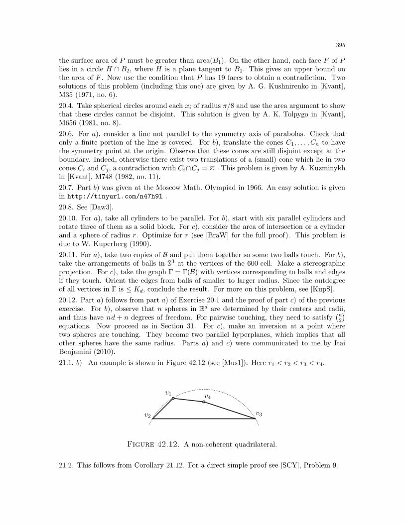
395

the surface area of P must be greater than area(B1). On the other hand, each face F of Plies in a circle H ∩ B2, where H is a plane tangent to B1. This gives an upper bound onthe area of F . Now use the condition that P has 19 faces to obtain a contradiction. Twosolutions of this problem (including this one) are given by A. G. Kushnirenko in [Kvant],M35 (1971, no. 6).

20.4. Take spherical circles around each xi of radius π/8 and use the area argument to showthat these circles cannot be disjoint. This solution is given by A. K. Tolpygo in [Kvant],M656 (1981, no. 8).

20.6. For a), consider a line not parallel to the symmetry axis of parabolas. Check thatonly a finite portion of the line is covered. For b), translate the cones C1, . . . , Cn to havethe symmetry point at the origin. Observe that these cones are still disjoint except at theboundary. Indeed, otherwise there exist two translations of a (small) cone which lie in twocones Ci and Cj, a contradiction with Ci∩Cj = ∅. This problem is given by A. Kuzminykhin [Kvant], M748 (1982, no. 11).

20.7. Part b) was given at the Moscow Math. Olympiad in 1966. An easy solution is givenin http://tinyurl.com/n47h9l .

20.8. See [Daw3].

20.10. For a), take all cylinders to be parallel. For b), start with six parallel cylinders androtate three of them as a solid block. For c), consider the area of intersection or a cylinderand a sphere of radius r. Optimize for r (see [BraW] for the full proof). This problem isdue to W. Kuperberg (1990).

20.11. For a), take two copies of B and put them together so some two balls touch. For b),take the arrangements of balls in S3 at the vertices of the 600-cell. Make a stereographicprojection. For c), take the graph Γ = Γ(B) with vertices corresponding to balls and edgesif they touch. Orient the edges from balls of smaller to larger radius. Since the outdegreeof all vertices in Γ is ≤ Kd, conclude the result. For more on this problem, see [KupS].

20.12. Part a) follows from part a) of Exercise 20.1 and the proof of part c) of the previousexercise. For b), observe that n spheres in Rd are determined by their centers and radii,and thus have nd + n degrees of freedom. For pairwise touching, they need to satisfy

(n2

)

equations. Now proceed as in Section 31. For c), make an inversion at a point wheretwo spheres are touching. They become two parallel hyperplanes, which implies that allother spheres have the same radius. Parts a) and c) were communicated to me by ItaiBenjamini (2010).

21.1. b) An example is shown in Figure 42.12 (see [Mus1]). Here r1 < r2 < r3 < r4.

v1

v2 v3

v4

Figure 42.12. A non-coherent quadrilateral.

21.2. This follows from Corollary 21.12. For a direct simple proof see [SCY], Problem 9.

396

21.4. The proof follows roughly along the same lines as the proof of Theorem 21.7. In thiscase one needs to consider the set of points at equal distance to 3 or more lines and provethat this is a binary tree.

21.6. See [Weg3].

21.10. For b), take an immersed closed curve C in Figure 9 in [Arn2]. Inscribe an equilateralpolygon Q and the same polygon Q′ with a shifted order of vertices.

21.11. See [OT1].

21.12. This is a discrete analogue of a result by Ghys (see [OT1] and references therein). Tosee a connection to the four vertex theorem, consider a polygon Q ⊂ R2 with vertices v1 =(x1, y1), . . . , vn = (xn, yn). For every i, consider a unique projective linear transformationϕi : RP1 → RP1, which maps xi−1, xi and xi+1 into yi−1, yi and yi+1, respectively. Denoteby Γ the graph (x, ϕ(x)) of function ϕ. Graph Γ now plays the role of circumscribed circlessince by definition it contains vi−1, vi and vi+1. Now check that αi− βi is a local minimumor maximum is the cyclic sequence if and only if the vertices vi−2 and vi+2 of Q lie on thesame side of Γ.

21.13. Part a) is a classical result of Szego (1920) and Suss (1924). We refer to [Ball] forthe related results and the references.

22.1. This proof is given in [A2, §9.1]. For a), see Figure 36.1. For b), take the signed areaof triangles spanned by the origin and the edges of P . For c), translate P so that the originin inside and differentiate the area:

2 · area(Pt)′ = (h1 ℓ

′1 + . . .+ hnℓ

′n) + (h′1 ℓ1 + . . . + h′nℓn).

On the other hand, area(Pt)′ = h′1 ℓ1 + . . . + h′nℓn by definition of the area, which implies

that area(Pt)′ = h1 ℓ

′1 + . . . + hnℓ

′n. Since area(Pt)

′ = 0 by assumption, and hi > 0 byconstruction, we conclude that some ℓ′i must be negative.For d), suppose vertices v and w separate the increasing and decreasing edges in P . Placethe origin in the intersection of the lines supporting P at v and w. Now all hi ℓ

′i have the

same sign in the expression for area(Pt)′, a contradiction.

22.3. Two proofs are given in [OR].

22.4. In part a) use the arm lemma (Lemma 22.3) and in b) use the extended arm lemma(Exercise 22.3). The proofs are given in [OR, ORS].

23.1. Consider separately all pairs of convex polygons in Y and then take a sum.

23.3. Part a) is a classical result on crossing numbers which can be found in [PacA, §14]and [Mat1, §4.3]. Part b) was proved in [AloG].

23.5. For b), see [Hal4]. For parts c) and d), see [Oza1].

23.6. This is studied in [Oza].

23.7. An involved version of this result is proved in [BolG], where it was proved by usingthe cut locus construction and deformations of polygons.

23.8. For a), an elegant smooth example is given in [Mor]. For b), see [Heil].

23.9. This is proved in [Hal3] via reduction to the smooth case.

23.10. This exercise follows closely [Carv].

23.11. The first explicit construction of a “stuck unknot” (space hexagon which cannotbe rigidly flatten) was constructed in [CanJ]. Another example is given in Figure 42.13(see [Tou]).

23.12. This is proved in [CocO].

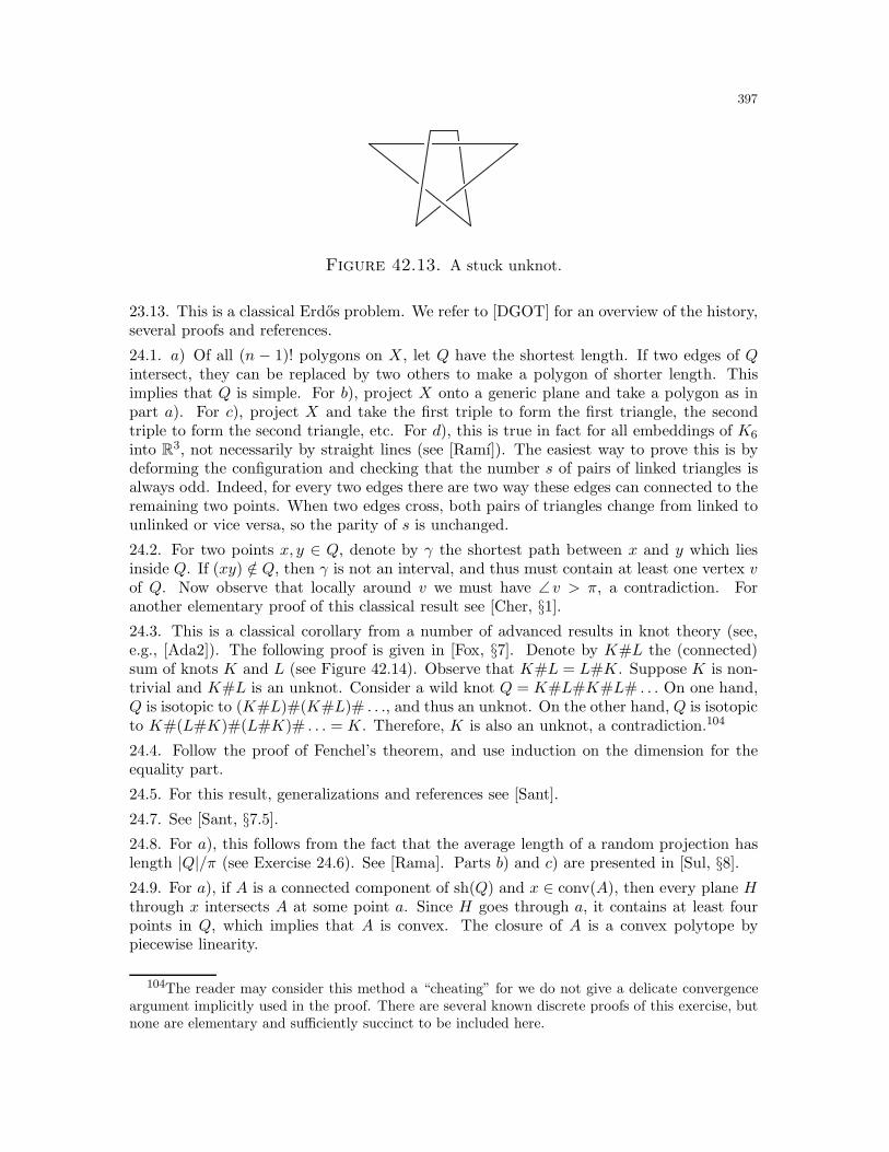
397

Figure 42.13. A stuck unknot.

23.13. This is a classical Erdos problem. We refer to [DGOT] for an overview of the history,several proofs and references.

24.1. a) Of all (n − 1)! polygons on X, let Q have the shortest length. If two edges of Qintersect, they can be replaced by two others to make a polygon of shorter length. Thisimplies that Q is simple. For b), project X onto a generic plane and take a polygon as inpart a). For c), project X and take the first triple to form the first triangle, the secondtriple to form the second triangle, etc. For d), this is true in fact for all embeddings of K6

into R3, not necessarily by straight lines (see [Ramı]). The easiest way to prove this is bydeforming the configuration and checking that the number s of pairs of linked triangles isalways odd. Indeed, for every two edges there are two way these edges can connected to theremaining two points. When two edges cross, both pairs of triangles change from linked tounlinked or vice versa, so the parity of s is unchanged.

24.2. For two points x, y ∈ Q, denote by γ the shortest path between x and y which liesinside Q. If (xy) /∈ Q, then γ is not an interval, and thus must contain at least one vertex vof Q. Now observe that locally around v we must have ∠ v > π, a contradiction. Foranother elementary proof of this classical result see [Cher, §1].

24.3. This is a classical corollary from a number of advanced results in knot theory (see,e.g., [Ada2]). The following proof is given in [Fox, §7]. Denote by K#L the (connected)sum of knots K and L (see Figure 42.14). Observe that K#L = L#K. Suppose K is non-trivial and K#L is an unknot. Consider a wild knot Q = K#L#K#L# . . . On one hand,Q is isotopic to (K#L)#(K#L)# . . ., and thus an unknot. On the other hand, Q is isotopicto K#(L#K)#(L#K)# . . . = K. Therefore, K is also an unknot, a contradiction.104

24.4. Follow the proof of Fenchel’s theorem, and use induction on the dimension for theequality part.

24.5. For this result, generalizations and references see [Sant].

24.7. See [Sant, §7.5].

24.8. For a), this follows from the fact that the average length of a random projection haslength |Q|/π (see Exercise 24.6). See [Rama]. Parts b) and c) are presented in [Sul, §8].

24.9. For a), if A is a connected component of sh(Q) and x ∈ conv(A), then every plane Hthrough x intersects A at some point a. Since H goes through a, it contains at least fourpoints in Q, which implies that A is convex. The closure of A is a convex polytope bypiecewise linearity.

104The reader may consider this method a “cheating” for we do not give a delicate convergenceargument implicitly used in the proof. There are several known discrete proofs of this exercise, butnone are elementary and sufficiently succinct to be included here.

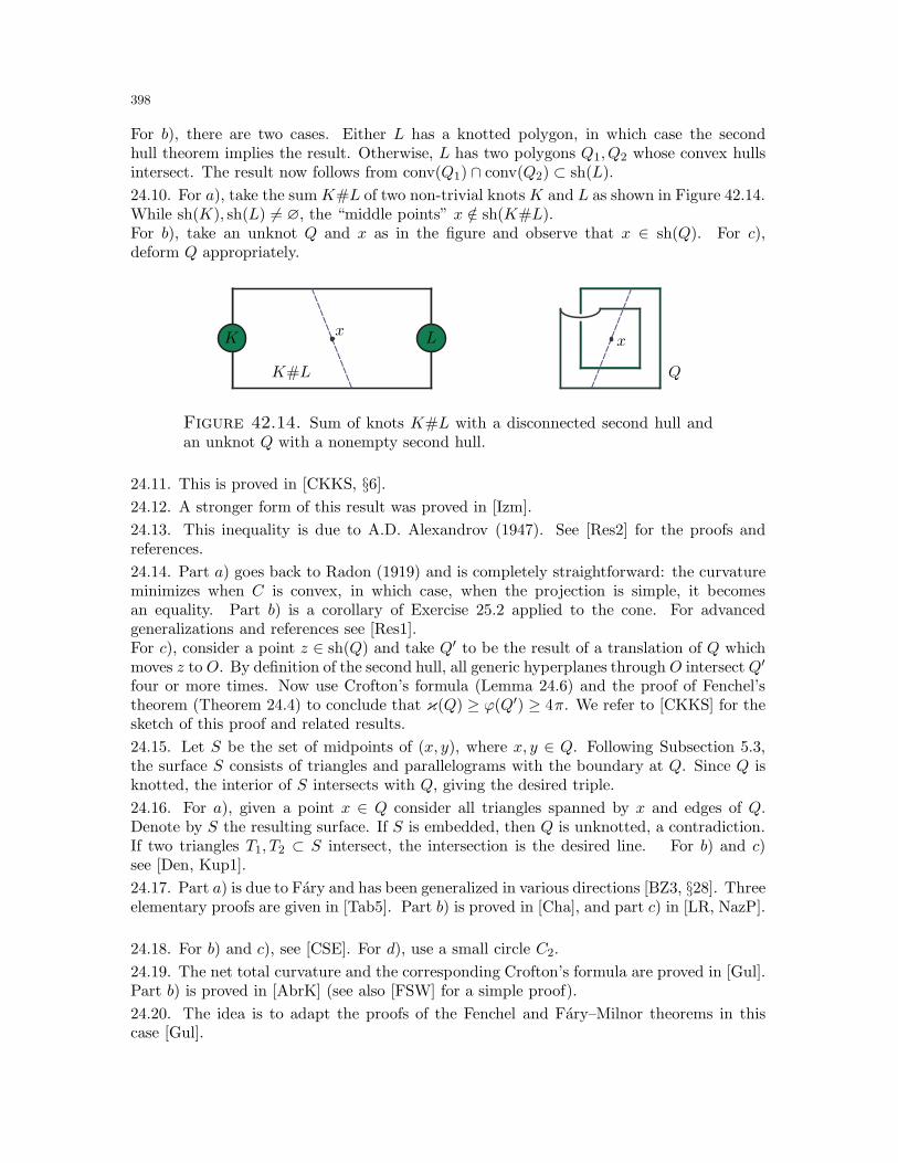
398

For b), there are two cases. Either L has a knotted polygon, in which case the secondhull theorem implies the result. Otherwise, L has two polygons Q1, Q2 whose convex hullsintersect. The result now follows from conv(Q1) ∩ conv(Q2) ⊂ sh(L).

24.10. For a), take the sum K#L of two non-trivial knots K and L as shown in Figure 42.14.While sh(K), sh(L) 6= ∅, the “middle points” x /∈ sh(K#L).For b), take an unknot Q and x as in the figure and observe that x ∈ sh(Q). For c),deform Q appropriately.

K L

QK#L

xx

Figure 42.14. Sum of knots K#L with a disconnected second hull andan unknot Q with a nonempty second hull.

24.11. This is proved in [CKKS, §6].

24.12. A stronger form of this result was proved in [Izm].

24.13. This inequality is due to A.D. Alexandrov (1947). See [Res2] for the proofs andreferences.

24.14. Part a) goes back to Radon (1919) and is completely straightforward: the curvatureminimizes when C is convex, in which case, when the projection is simple, it becomesan equality. Part b) is a corollary of Exercise 25.2 applied to the cone. For advancedgeneralizations and references see [Res1].For c), consider a point z ∈ sh(Q) and take Q′ to be the result of a translation of Q whichmoves z to O. By definition of the second hull, all generic hyperplanes through O intersect Q′

four or more times. Now use Crofton’s formula (Lemma 24.6) and the proof of Fenchel’stheorem (Theorem 24.4) to conclude that κ(Q) ≥ ϕ(Q′) ≥ 4π. We refer to [CKKS] for thesketch of this proof and related results.

24.15. Let S be the set of midpoints of (x, y), where x, y ∈ Q. Following Subsection 5.3,the surface S consists of triangles and parallelograms with the boundary at Q. Since Q isknotted, the interior of S intersects with Q, giving the desired triple.

24.16. For a), given a point x ∈ Q consider all triangles spanned by x and edges of Q.Denote by S the resulting surface. If S is embedded, then Q is unknotted, a contradiction.If two triangles T1, T2 ⊂ S intersect, the intersection is the desired line. For b) and c)see [Den, Kup1].

24.17. Part a) is due to Fary and has been generalized in various directions [BZ3, §28]. Threeelementary proofs are given in [Tab5]. Part b) is proved in [Cha], and part c) in [LR, NazP].

24.18. For b) and c), see [CSE]. For d), use a small circle C2.

24.19. The net total curvature and the corresponding Crofton’s formula are proved in [Gul].Part b) is proved in [AbrK] (see also [FSW] for a simple proof).

24.20. The idea is to adapt the proofs of the Fenchel and Fary–Milnor theorems in thiscase [Gul].

399

24.21. Part a) was proved in [Bes1]. For b), take three symmetric geodesic arcs from theNorth Pole of length π − ε and add a small geodesic equilateral triangle around the SouthPole. The resulting net has total length 3π+O(ε), where ε > 0. Part c) is a generalizationof a) given in [Crof].

25.3. Region A contains all vertices of P , has n = 2 |E| vertices, while ∂A has r = |F|connected components. Observe that every angle of A is a complement of the correspondingface angle to 2π, which gives

α(A) = n · (2π) −∑

v∈Vα(v) = (n − |V |) · 2π +

∑

v∈V(2π − α(v))

= 2π · (2|E| − |V |) +∑

v∈Vω(v) = 4π · |E| − 2π · |V | + 4π .

On the other hand, by the previous exercise, we have α(A) = (2|E|+ 2|F|−4) ·π. Togetherthese two equations imply Euler’s formula.

25.5. For a), consider the dual cones C∗ and D∗. Use the supporting hyperplanes to showthat C∗ ⊃ D∗. Conclude from here that ω(C) = σ(C∗) ≥ σ(D∗) = ω(D∗).

25.6. For a), note that the centrally symmetric faces have at least four vertices. Now useEuler’s formula. For b), consider the Minkowski sum of n vectors in convex position (takee.g., the side edges of a symmetric n-pyramid). The resulting zonotope has at least n faces,all parallelograms (see Exercise 7.16).

25.8. For b), here is a solution from [Grub, §15.1]. Denote by ai the number of vertices ofdegree i, and by fi the number of i-sided faces. For the numbers n, m and k of vertices,edges and faces, respectively, we have n = a3 + a4 + a5 + . . . , k = f3 + f4 + f5 + . . . , and2m = 3a3 + 4a4 + 5a5 + . . . = 3f3 + 4f4 + 5f5 + . . . By Euler’s formula, we conclude:

8 = (4n− 2m) + (4k − 2m) = (4a3 + 4a4 + 4a5 + . . . − 3a3 − 4a4 − 5a5 − . . .)+ (4f3 + 4f4 + 4f5 + . . . − 3f3 − 4f4 − 5f5 − . . .) ≤ a3 + f3 .

25.9. For a), observe that the curvature of all vertices are bounded: ωi ≤ π/2. Now theGauss–Bonnet theorem implies the result. Part b) is analogous. Note that both boundsare tight: take the cube and the icosahedron, respectively.

25.10. Use Girard’s formula to write each solid angle in terms of dihedral angles. Summingover all vertices, each dihedral angle will be counted twice. Then use Euler’s formula.

25.11. This is a dual result to the Gauss–Bonnet theorem (Theorem 25.3).

25.12. (ii)⇒ (i) Write out equations for the edge lengths.(iii) ⇒ (i) From the Gauss–Bonnet theorem (Theorem 25.3), conclude that the curvatureof each vertex is equal to π. Now write out the equations for the angle sums around eachvertex and inside each face.(iv)⇒ (i) Use an argument based on Subsection 25.3.(v)⇒ (iv) Write out equations for the solid angles in terms of dihedral angles.

25.13. This follows from Euler’s formula. See Subsection 26.3 for the proof.

25.14. This is a restatement of Euler’s formula. It is proved in [Gla] (see also [GGT, §2]).

25.15. Both parts easily follow from Exercise 25.14. For a), if there are no sinks, sourcesand faces with oriented cycles, then the index of every vertex and face is ≤ 0, while by theformula in the exercise, their sum is zero, a contradiction. Alternatively, one can provepart a) in the same manner as Lemma 32.7. Since there are no sinks in the graph, everyoriented path can be extended until it self-intersects. If the resulting cycle is not along a

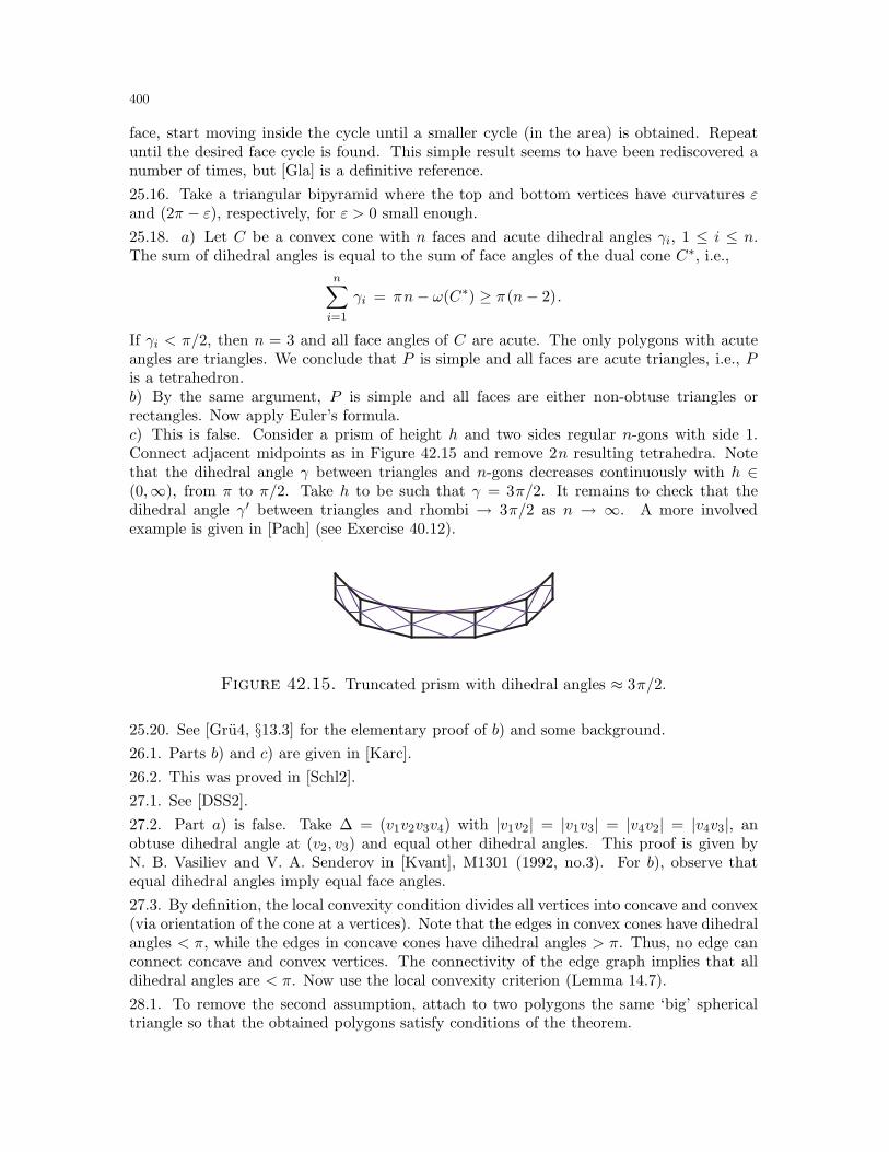
400

face, start moving inside the cycle until a smaller cycle (in the area) is obtained. Repeatuntil the desired face cycle is found. This simple result seems to have been rediscovered anumber of times, but [Gla] is a definitive reference.

25.16. Take a triangular bipyramid where the top and bottom vertices have curvatures εand (2π − ε), respectively, for ε > 0 small enough.

25.18. a) Let C be a convex cone with n faces and acute dihedral angles γi, 1 ≤ i ≤ n.The sum of dihedral angles is equal to the sum of face angles of the dual cone C∗, i.e.,

n∑

i=1

γi = πn− ω(C∗) ≥ π(n− 2).

If γi < π/2, then n = 3 and all face angles of C are acute. The only polygons with acuteangles are triangles. We conclude that P is simple and all faces are acute triangles, i.e., Pis a tetrahedron.b) By the same argument, P is simple and all faces are either non-obtuse triangles orrectangles. Now apply Euler’s formula.c) This is false. Consider a prism of height h and two sides regular n-gons with side 1.Connect adjacent midpoints as in Figure 42.15 and remove 2n resulting tetrahedra. Notethat the dihedral angle γ between triangles and n-gons decreases continuously with h ∈(0,∞), from π to π/2. Take h to be such that γ = 3π/2. It remains to check that thedihedral angle γ′ between triangles and rhombi → 3π/2 as n → ∞. A more involvedexample is given in [Pach] (see Exercise 40.12).

Figure 42.15. Truncated prism with dihedral angles ≈ 3π/2.

25.20. See [Gru4, §13.3] for the elementary proof of b) and some background.

26.1. Parts b) and c) are given in [Karc].

26.2. This was proved in [Schl2].

27.1. See [DSS2].

27.2. Part a) is false. Take ∆ = (v1v2v3v4) with |v1v2| = |v1v3| = |v4v2| = |v4v3|, anobtuse dihedral angle at (v2, v3) and equal other dihedral angles. This proof is given byN. B. Vasiliev and V. A. Senderov in [Kvant], M1301 (1992, no.3). For b), observe thatequal dihedral angles imply equal face angles.

27.3. By definition, the local convexity condition divides all vertices into concave and convex(via orientation of the cone at a vertices). Note that the edges in convex cones have dihedralangles < π, while the edges in concave cones have dihedral angles > π. Thus, no edge canconnect concave and convex vertices. The connectivity of the edge graph implies that alldihedral angles are < π. Now use the local convexity criterion (Lemma 14.7).

28.1. To remove the second assumption, attach to two polygons the same ‘big’ sphericaltriangle so that the obtained polygons satisfy conditions of the theorem.

401

28.2. a) Let Pt = P +Bt, where Bt is a ball of radius t, so that P0 = P . Observe that

area(Pt) = area(P ) + t ·∑

e

ℓe (π − γe) + 4πt2.

On the other hand, since Pt ⊂ BR+t , we have area(Pt) ≤ area(BR+t) = 4π(R + t)2.Therefore,

area(P ) + t ·∑

e

ℓe (π − γe) + 4πt2 ≤ 4π(R + t)2.

Letting t→∞, we obtain the result.b) Define Pt = P +Bt, Qt = Q+Bt, and use area(Pt) ≤ area(Qt) as t→∞.

28.4. See [CSE].

28.6. For a), move a vertex of a tetrahedron along one of the edges. Check the formula by adirect calculation. Obtain the general formula from an (infinitesimal) composition of suchtransformations. For b), triangulate the polyhedron enclosed by the surface, apply a) anduse the additivity of the Schlafli formula.

28.8 and 28.9. See [Kor2, Kor1].

30.1. For a), let us first prove that tightness implies both conditions. Suppose the edgecondition fails for the edge e = (v,w) ⊂ conv(P ), where v and w are vertices in P . Thenthe plane along e and separating from other vertices of P divides P into at least threeparts. Similarly, if the vertex condition fails at v /∈ ∂conv(P ), we can separate v from othervertices by a plane near v. Now observe that every such plane divides P into three or moreparts. In the opposite direction, suppose plane L intersects P and creates three or moreconnected components. Choose a side with two or more such components. Recall that thegraph of edges of conv(P ) lying on one side of L is connected (see Exercise 8.3). If allcomponents contain vertices in conv(P ), then by the edge condition all components mustbe connected to each other via the edges of conv(P ), a contradiction. Finally, if Q ⊂ P is acomponent without vertices in conv(P ), then the furthest from L vertex v ∈ Q violates thevertex condition. This result is due to Banchoff, while our proof follows [Kuh, §2].b) The edge condition is clearly insufficient as evident from a non-convex bipyramid inFigure 30.1. Similarly, the vertex condition holds for a non-tight Jessen’s icosahedron (seeExercise 19.17).d) If an intersection Q = P ∩L of P with a plane L is disconnected, then P has at least threeconnected components, since n curves separate the surface homeomorphic to a sphere inton+1 components. Now, if every intersection is connected, the interior of A is a contractiblepolygon, and the convexity criterion (Exercise 1.25) implies the result.

30.2. See [Spi] for one such construction.

30.3. Remember, it is very hard to make a flexible polyhedron!

30.4. The first part remains an open problem despite numerous attempts (and incorrectconstructions). The second part is a conjecture of Stachel [St1].

31.2. See [FedP, §7.5].

31.3. Parts a), b), c) are due to Robbins, who also conjectured parts d) and e, which wereproved in [FedP]. See [Pak4] for a survey and [Var1] for an independent approach.

31.4. See [Con1].

31.5. For a), let D be the square length of the diagonal and let R be the squared radius.Clearly, D/4 + R = L is a constant given by the squared side edge length. Now make a

402

substitution of (L−D/4) into the Sabitov polynomial for R. For b), use the fact that Znhas exponentially many realizations. For c), further details and references see [FedP].

31.6. a) Use ℓ12 = ℓ23 = ℓ13 = 2 and ℓ01 = ℓ02 = ℓ03 = 1 + ε, for ε > 0 small enough. b)Consider ∆,∆′ ⊂ R3 with edge lengths

ℓ01 = ℓ02 = ℓ03 = 1 , ℓ13 = ℓ23 =√

2 , ℓ12 = ε,

ℓ′01 = ℓ′02 = ℓ′03 = 1 , ℓ′12 = ℓ′23 =√

2 , ℓ′13 = ε,

where ε > 0 is small enough. Check that ∆,∆′ with such edge lengths exist, and that thereis no tetrahedron with (ℓij + ℓ′ij)/2 edge lengths. For c) and the references see [Riv].

34.8. Parts a) and b) are proved in [Mon1]. This technique was later extended in [Mon2]to prove c) and d). Parts e) and f) are proved in [Pok]. See [Ste2] for a survey.

32.2. This result is due to Pogorelov [Pog6].

32.3. From the contrary, suppose there exists a continuous deformation of C ′. Denote by Gthe graph of P . As in the proof of the Cauchy theorem, consider a subgraph H ⊂ G ofedges where the dihedral angles change. Check that every vertex of H has degree at least 4.Use Exercise 25.7 to conclude that at least eight triangular faces of H (as a planar graph)are triangular. In the other direction, show that even-sided faces of G cannot subdividethese triangles. The second part is similar. See [DSS1] for details and references.

32.4. This can be proved using the combinatorial approach in Subsection 32.3. See [A2,§10.3] for the original proof.

33.2. Consider the following deformation Pt of the coordinates of Jessen’s orthogonalicosahedron:

(±2,±(1 + t), 0

),(±(1 + t), 0,±2

),(0,±2,±(1 + t)

).

Observe that the lengths of the long edges are unchanged under the deformation, while thelengths of the short edges are

√(1− t)2 + (1 + t)2 =

√2 + 2t2 =

√2 + O(t2) as t→ 0.

This implies that the polyhedron P0 is not infinitesimally rigid. Continuous rigidity followsfrom the second order rigidity. First, check that the rigidity matrix has corank 1, i.e., theabove first order deformation is the only possible (up to scaling). Then check that thesecond order terms implied by O(t2) are strictly positive, for all t 6= 0.

33.5. Part d) is a proved in [Con3]. See [Con5, ConS, IKS] for more second order rigidity.

33.7 and 33.8. See [RotW, §6, 7].

33.10. See [Luo] for the proof, extensions and references.

31.7. For a), consider normals u i to the faces. Observe that ∠u iuj = π − γij. Now takew i = area(Fi) · u i, where Fi is the face of ∆ which does not contain vertex vi. Recallthat w1 + w2 + w3 + w4 = 0 (see Proposition 36.1). Thus there exists a closed spacequadrilateral Q with edges w i, and the sum of angles in Q is ≤ 2π. Since the sum of anglesin Q is equal to γ12 + γ23 + γ34 + γ14, we obtain the result.For b), observe that γ12 + γ13 + γ14 > π, since the curvature of the dual cone ω(C∗

1 ) =(π − γ12) + (π − γ13) + (π − γ14) < 2π. Adding such inequalities for all four vertices weobtain the lower bound. The upper bound follows by averaging of the inequalities in a).For c), we have:

∑

ij

cos γij =∑

ij

−〈u i,uj〉 = 2− 1

2〈u1 + u2 + u3 + u4,u1 + u2 + u3 + u4〉 = 2 − |r |

2

2,

403

where r = u1 + u2 + u3 + u4. Since |r | ≤ 2, we immediately obtain both lower and upperbounds. For d), observe that the equality holds only if r = 0. From the proof of theprevious exercise, we conclude that ∆ is equihedral.Parts a)-d) are given by I. F. Sharygin in [Kvant], M353 (1976, no. 7). For part e), show thatone can monotonically increase the dihedral angles to obtain dihedral angles of a Euclideanpolytope in the limit.

33.11. This is a small special case of Schramm’s theorem in [Schra]. The proof uses anadvanced generalization of inversions and a similar inversion counting argument.

34.1. For part a), see [Hada, § 255]. For part b), see [FedP, §8].

34.2. For b), write both sides of the Cayley-Menger determinants mod 8. Part c) was ona Putnam Mathematical Competition in 1993.

34.3. For a), take two 4-tuples of points in the plane:

|a1a2| = |a1a3| =√

2, |a2a3| = 2, |a2a4| = |a3a4| =√

10, |a1a4| = 4.

|b1b2| = |b3b4| =√

2, |b1b3| = 2, |b1b4| = |b2b3| =√

10, |b2b4| = 4.

For b), fix the first coordinates of all points ai = (xi, yi), 1 ≤ i ≤ n. For every six distanceswhich can potentially form a flat 4-tuple, write out their Cayley-Menger determinant. Checkthat the resulting polynomial equations on yi are nontrivial unless these distances form theusual 4-point pattern. Conclude that for almost all values of yi the set ai has no equivalentand non-congruent sets. See [BouK] for this and further results.

34.6. This was first proved in [Var1]. A simple proof using the theory of places is givenin [Con6] (see also [Pak4]).

35.1. For c), use the fact that σ(C) is monotone on cones C. See [Pog3, §7.7] for the detailsand further generalizations.

35.5. Take a set of points b1, . . . , bk such that polygon B = [b1 . . . bk] contains all ai in itsrelative interior. Let Z = ∂B. For every ǫ > 0, use use Theorem 35.7 to obtain Pǫ onn + k vertices ai and bj, with boundary Z and curvatures ω1 − ǫ, . . . , ωn − ǫ. Let P ′

ǫ be ashifted Pǫ with the sum of heights of interior vertices equal to 0. Check that P ′

ǫ convergesto the desired convex cap as ǫ→ 0.

35.8. For a), we implicitly use combinatorics of P when lifting vi, since for ε > 0 smallenough the combinatorics is unchanged. For a greedy variational algorithm, start with theupper surface of the convex hull conv(Z). Take the smallest i such that νi < ωi. Lift it upuntil the equality is reached. Repeat. For b), presumably the exponential upper bound onthe number of full triangulations must play a role (see Exercise 14.7).

35.9. Find an appropriate direction of rays and use Theorem 35.4. This result is obtainedin [Zil] (cf. [Thu, §7]).

36.2. Compare the corresponding faces in polytopes P , Q = 12(P + P ′) and P ′. Since

the normals to the corresponding faces are equal, these polygons are parallel (have parallelcorresponding edges). Here we allow zero edge lengths in case the parallel edge is notpresent. Observe that the edge lengths in Q are the averages of the corresponding edgelengths in P and P ′. Write signs (+), (0) and (−) on the edges of Q (including zero lengthedges), if their edge lengths in P are greater, equal or smaller than that of edges in P ′,respectively.

Note that there are two types of faces in Q: those coming from faces in one polytope anda vertex from another, and those coming from one edge in each. Apply Alexandrov’s lemmato show that around each face of Q, either all signs are zero or there are four sign changes.

404

Take the dual graph to the graph of Q and keep the same signs, so that there are at leastfour sign changes around every vertex. Modify counting argument in Subsection 26.3, toconclude that all signs must be zero.

36.3. In notation of Subsection 36.2, define a map ϕ : P → Z. Prove that Z ⊂ W+ is aconvex polyhedron by a direct argument (cf. the proof of Lemma 35.3). Similarly, provedirectly that P is connected. Consider only polytopes P ∈ P of volume 1. In the topologicallemma, the injectivity follows from the Alexandrov theorem and the continuity is trivial.To show that ϕ is proper, check that the limit polyhedron cannot become unbounded ordegenerate. A complete proof is given in [A2, §6.3].

36.5. Note that in the proof we use the equal facet areas only to avoid F ∗k ⊂ Fk, and other

conditions can be used in its place. Use monotonicity of the perimeter, surface area, andthe mean curvature (see Exercises 7.11 and 28.2).

36.9. For a), consider normals u i to the faces and use the equation in Proposition 36.1to conclude that their sum is zero. Check that the resulting 2-dimensional family of(u1,u2,u3,u4) (up to rotations around O), is the same as the family of normals ofequihedral tetrahedra.For b), recall that equihedral tetrahedra have equal opposite edges (see Exercise 25.12).From a), this implies that all non-adjacent edges have equal length. This easily implies theresult.

36.10. Much of this exercise is due to Shephard (1963). See proofs and references in [McM1,Mey]. Part e) is given in [Kall].

36.12. For a), translate P by a vector w . We have:

υ(P,P ′ + w) =n∑

i=1

(z1 + 〈w ,u i〉

)a′i =

n∑

i=1

z1a′i +

⟨w ,

n∑

i=1

a′iu i

⟩= υ(P,P ′),

since the second term is zero. See [A2, §7.2] for the rest of this exercise.

36.13. Here υ(P,P ′) is the usually called the mixed volume vol(P,P ′, . . . , P ′), and theexercise gives an equivalent way to state the Brunn–Minkowski inequalities. This approachleads to the further inequalities, as discussed in [BonF, BZ3, Schn2].

36.14. By the uniqueness part of Theorem 36.2, polytope P is a translate of (−P ). Thisimplies the result.

36.15. A concise proof of part a is given in [Grub, §18.2].

36.16. For d) and e) see [A2, §7.1]. The truncated octahedron tiles the space and has 14faces (see Exercise 16.6). The upper bound in f is due to Minkowski. We refer to [Grub,§32.2] for the proofs, references and the context.

36.18. See [BezB].

36.19. This example was recently constructed in [Pan].

37.1. For a), cut the surface of a convex cap by a hyperplane and combine two copies toobtain a convex polytope with reflection symmetry. Show that this can be done intrinsically.For b), see [A2, §4.4].

37.4. See [ADO].

37.5. Part c) was proved by Harer and Zagier in (1986). See combinatorial proofs in [GouN,Lass].

37.8. For a), it suffices to check that the sum of angles around each vertex is < 2π. Use thelaw of cosines to obtain stability result for the angles (e.g., ε < 0.01 easily works). For b),

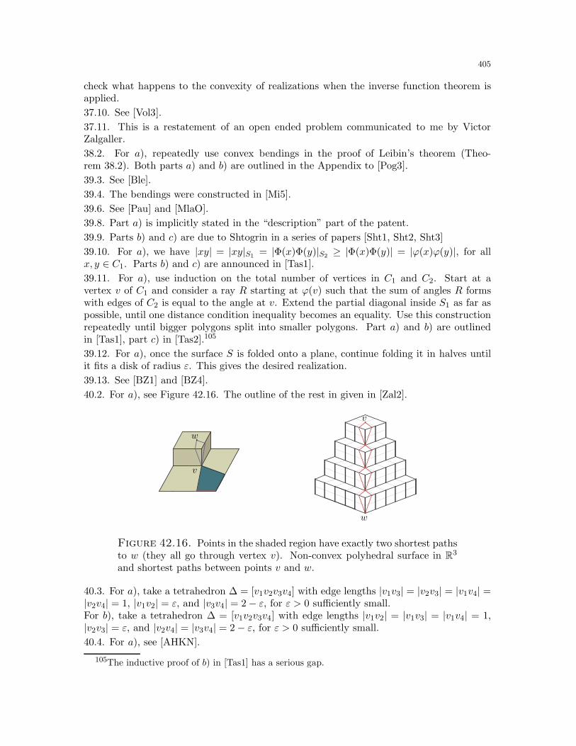
405

check what happens to the convexity of realizations when the inverse function theorem isapplied.

37.10. See [Vol3].

37.11. This is a restatement of an open ended problem communicated to me by VictorZalgaller.

38.2. For a), repeatedly use convex bendings in the proof of Leibin’s theorem (Theo-rem 38.2). Both parts a) and b) are outlined in the Appendix to [Pog3].

39.3. See [Ble].

39.4. The bendings were constructed in [Mi5].

39.6. See [Pau] and [MlaO].

39.8. Part a) is implicitly stated in the “description” part of the patent.

39.9. Parts b) and c) are due to Shtogrin in a series of papers [Sht1, Sht2, Sht3]

39.10. For a), we have |xy| = |xy|S1= |Φ(x)Φ(y)|S2

≥ |Φ(x)Φ(y)| = |ϕ(x)ϕ(y)|, for allx, y ∈ C1. Parts b) and c) are announced in [Tas1].

39.11. For a), use induction on the total number of vertices in C1 and C2. Start at avertex v of C1 and consider a ray R starting at ϕ(v) such that the sum of angles R formswith edges of C2 is equal to the angle at v. Extend the partial diagonal inside S1 as far aspossible, until one distance condition inequality becomes an equality. Use this constructionrepeatedly until bigger polygons split into smaller polygons. Part a) and b) are outlinedin [Tas1], part c) in [Tas2].105

39.12. For a), once the surface S is folded onto a plane, continue folding it in halves untilit fits a disk of radius ε. This gives the desired realization.

39.13. See [BZ1] and [BZ4].

40.2. For a), see Figure 42.16. The outline of the rest in given in [Zal2].

v

v

w

w

Figure 42.16. Points in the shaded region have exactly two shortest pathsto w (they all go through vertex v). Non-convex polyhedral surface in R3

and shortest paths between points v and w.

40.3. For a), take a tetrahedron ∆ = [v1v2v3v4] with edge lengths |v1v3| = |v2v3| = |v1v4| =|v2v4| = 1, |v1v2| = ε, and |v3v4| = 2− ε, for ε > 0 sufficiently small.For b), take a tetrahedron ∆ = [v1v2v3v4] with edge lengths |v1v2| = |v1v3| = |v1v4| = 1,|v2v3| = ε, and |v2v4| = |v3v4| = 2− ε, for ε > 0 sufficiently small.

40.4. For a), see [AHKN].

105The inductive proof of b) in [Tas1] has a serious gap.

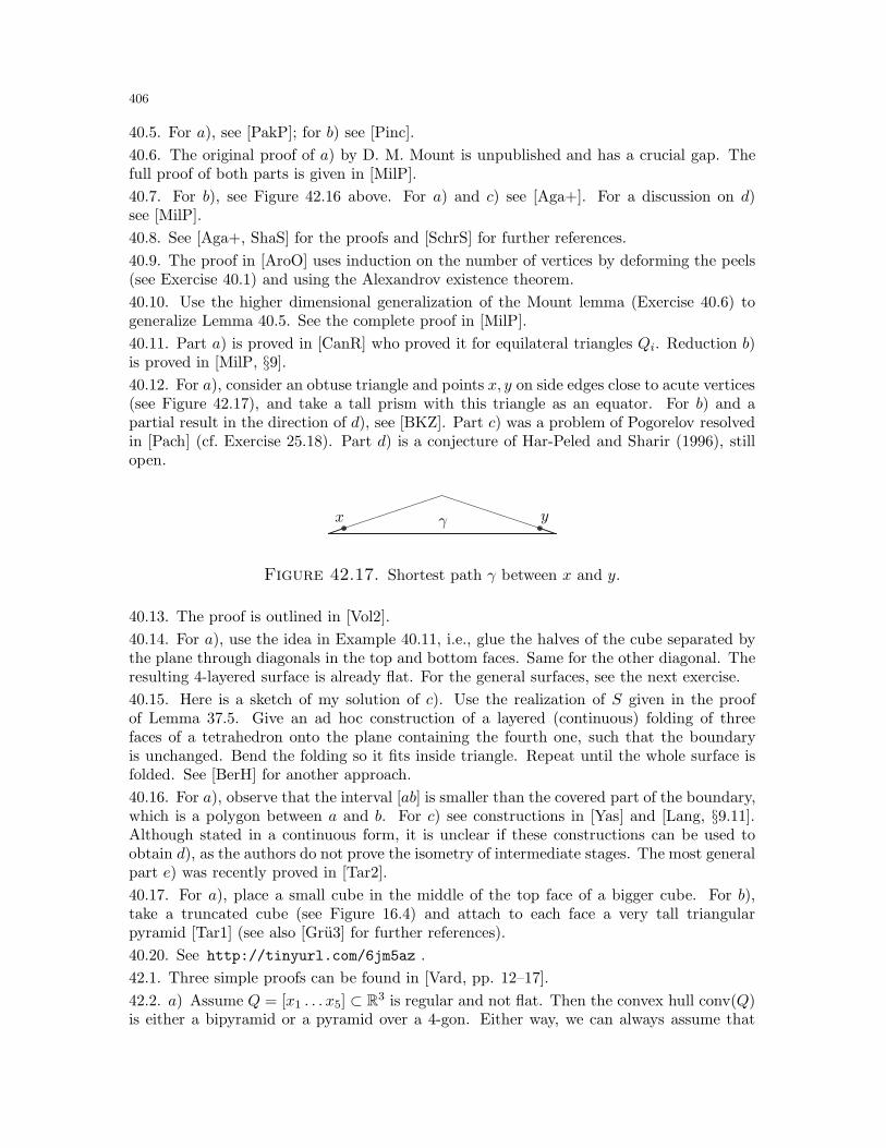
406

40.5. For a), see [PakP]; for b) see [Pinc].

40.6. The original proof of a) by D. M. Mount is unpublished and has a crucial gap. Thefull proof of both parts is given in [MilP].

40.7. For b), see Figure 42.16 above. For a) and c) see [Aga+]. For a discussion on d)see [MilP].

40.8. See [Aga+, ShaS] for the proofs and [SchrS] for further references.

40.9. The proof in [AroO] uses induction on the number of vertices by deforming the peels(see Exercise 40.1) and using the Alexandrov existence theorem.

40.10. Use the higher dimensional generalization of the Mount lemma (Exercise 40.6) togeneralize Lemma 40.5. See the complete proof in [MilP].

40.11. Part a) is proved in [CanR] who proved it for equilateral triangles Qi. Reduction b)is proved in [MilP, §9].

40.12. For a), consider an obtuse triangle and points x, y on side edges close to acute vertices(see Figure 42.17), and take a tall prism with this triangle as an equator. For b) and apartial result in the direction of d), see [BKZ]. Part c) was a problem of Pogorelov resolvedin [Pach] (cf. Exercise 25.18). Part d) is a conjecture of Har-Peled and Sharir (1996), stillopen.

x yγ

Figure 42.17. Shortest path γ between x and y.

40.13. The proof is outlined in [Vol2].

40.14. For a), use the idea in Example 40.11, i.e., glue the halves of the cube separated bythe plane through diagonals in the top and bottom faces. Same for the other diagonal. Theresulting 4-layered surface is already flat. For the general surfaces, see the next exercise.

40.15. Here is a sketch of my solution of c). Use the realization of S given in the proofof Lemma 37.5. Give an ad hoc construction of a layered (continuous) folding of threefaces of a tetrahedron onto the plane containing the fourth one, such that the boundaryis unchanged. Bend the folding so it fits inside triangle. Repeat until the whole surface isfolded. See [BerH] for another approach.

40.16. For a), observe that the interval [ab] is smaller than the covered part of the boundary,which is a polygon between a and b. For c) see constructions in [Yas] and [Lang, §9.11].Although stated in a continuous form, it is unclear if these constructions can be used toobtain d), as the authors do not prove the isometry of intermediate stages. The most generalpart e) was recently proved in [Tar2].

40.17. For a), place a small cube in the middle of the top face of a bigger cube. For b),take a truncated cube (see Figure 16.4) and attach to each face a very tall triangularpyramid [Tar1] (see also [Gru3] for further references).

40.20. See http://tinyurl.com/6jm5az .

42.1. Three simple proofs can be found in [Vard, pp. 12–17].

42.2. a) Assume Q = [x1 . . . x5] ⊂ R3 is regular and not flat. Then the convex hull conv(Q)is either a bipyramid or a pyramid over a 4-gon. Either way, we can always assume that

407

x1 and x4 lie on the same side of the plane spanned by x2, x3 and x5. By the assumptions,all diagonals in Q have equal length. Thus tetrahedra (x4x2x3x5) and (x1x2x3x5) arecongruent. Since x1 and x4 lie on the same side of the isosceles triangle (x2x3x5), weconclude that x1 and x4 are symmetric with respect to the plane bisecting (x2, x3). Thuspoints x1, x2, x3 and x4 lie in the same plane. The same argument shows that x5, x2, x3

and x4 lie on the same plane, and we obtain a contradiction. See [PraS], Problem 8.29.b) For even n, consider the regular n-antiprism and a polygon obtained by the side edges.For n odd, find a non-planar regular 7-gon and use induction. To see why this is true forodd n large enough, consider a long metal chain of small equilateral triangles attached asin the regular antiprism, but make the chain open and flexible along the edges. Clearly, wecan twist it and close it up if the chain is long enough.

42.4. This result is due to P. W. Jones (1990). We refer to [KenK] for an elegant presentationand references.

42.5. Take the longest edge. See [Shar], Problem 170.

While there is a large literature on the subject, there is no standard name for these tetra-hedra. We refer to [Arn3, pp. 2, 188–191] for the references, and to [PraS, §6.4] (seealso [Shar], Problem 304) for simple proofs of these and other basic results on equihedraltetrahedra. Let us mention that these tetrahedra are also called isosceles (see [Lee, The])and equifacial (see [HajW]). See also Exercise 10.4 for more on this.

42.8. Consider a hyperplane H ⊂ Rd defined by the equationx1

a1+ . . . +

xdad

= d.

Clearly, a ∈ H. Since a is an interior point, there exists a vertex v of P on the same sideof H as the origin O. We conclude:

viai≤ v1

a1+ . . . +

vdad≤ d.

This solution follows [SGK, §3.2].

42.10. See Problem 266 in [VasE].

42.11. The upper bound (2n − 4) is sharp. See the solution to Problem 8.6 in [PraS].

42.12. This is false (see [PraS], Problem 13.12). Check that two vertices on the same edgecan lie in C. Extend the planes of C to divide the space into 8 cones. Conclude that atleast one of them will have two vertices of the cube.

42.13. Part a) is proved in [Klee]. Part b), was originally proposed in [She2] (see also [CFG],section B10) and completely resolved in [CEG]. For c), start with a regular tetrahedronand add a vertex at distance ε from the barycenter of every face. Then add a vertex atdistance ε2 from the barycenter of every new face, etc. Repeat this O(n) times.

42.15. For a), the claim is false. Start with a unit circle C ⊂ R3 defined by x2 + y2 = 1and z = 0. Take a cone over C from a = (−1, 0, 1) and b = (−1, 0,−1). The resultingconvex body B has extremal points at C − (−1, 0, 0) and a, b. To make only countablymany extremal points, modify this example by taking a convex hull of a, b and a convergingsequence to (−1, 0, 0) of points in C. We are unaware of an elementary proof of b).

42.17. See [Zon2] for proofs, generalizations and references. For b), see also a hint on p. 74in [Tao].

42.18. This problem was given at the Moscow Math. Olympiad in 2008. See http://tinyurl.com/ma34td

for a complete solution.

408

42.19. a) Take a projection of a tetrahedron ∆ onto a plane L containing face (abc). Assumethe remaining vertex d is projected into the interior of (abc). Choose two lines ℓ1 = (ab)and ℓ2 ⊥ ℓ1. Rotate ∆ by an angle ǫ > 0 around ℓ1 and then around ℓ2. The new projectionis a triangle (a′b′c′) that fits inside (abc), for ǫ small enough.b) For the unit cube: the unit square projection fits inside the regular hexagonal projection

(with side√

2/3).c) For the regular octahedron with edge length 1: start with a unit square projection.Rotate the octahedron around a diagonal of the square by an angle ǫ > 0. Rotate theoctahedron now around the second diagonal by an angle ǫ2. The resulting projection fitsinside the unit square, for ǫ small enough.d) Although we have not checked, the regular icosahedron looks like a potential counterex-ample.

42.20. Part a) was proved by Kovalev (1984), while part c) was proved in [DML]. See [KosT]for a simple proof of a) and the references.

42.21. a) For Cd = (x1, . . . , xd), 0 ≤ xi ≤ 1, take a hyperplane x1 + . . . + xd = 2.For b), c) and d), see [JocP].

42.22. Use the fact that K3,3 is not planar. See [Sany] for details and generalization.

42.23. See [Pol]. The example of cuboctahedron shows that the bound is tight.

42.24. This is called the Szilassi polyhedron. It is easy to see that this is possible only if ithas 14 vertices and 28 edges. See http://tinyurl.com/2qqzgc for the references.

42.25. This construction is called the Csaszar polyhedron [Csa].

42.26. Let ∆ = (v1v2v3v4) and suppose (v1v2) is the longest edge. We have:

2|v1v2| ≤(|v1v3|+ |v2v3|

)+(|v1v4|+ |v2v4|

)=(|v1v3|+ |v1v4|

)+(|v2v3|+ |v2v4|

).

Therefore, either |v1v2| ≤ |v1v3|+ |v1v4|, or |v2v1| ≤ |v2v3|+ |v2v4|, as desired. The problemcomes from the Tournament of Towns in 1994 (see http://tinyurl.com/lk6he3)

42.27. An elegant proof of this is given in [GriL, §2].

42.28. Let v i = −−→x1xi and w i = −−−−→xixi+1, for all 1 ≤ i ≤ n. Clearly, v i = w1 + . . .+ w i−1. Byanalogy with the volume formula in Subsection 34.1, we have 2area(X) = |u |, where

u =n∑

i=1

v i × v i+1 =n∑

i=1

v i × (v i + w i) =n∑

i=1

v i ×w i

=

n∑

i=1

(w1 + . . . + w i−1)×w i =∑

i<j

w i ×w j .

Taking the norm of both sides immediately implies Sarron’s formula.

42.31. See [Eri].

42.32. For this and other properties of the polar sine function see [LerW].

42.33. This is a result of Lagrange (1783). See [GooT] for a short proof.

42.36. See [Kah].

42.38. For b), this is false. Take a quadrilateral inscribed into a circle with O as a center.Now permute triangles spanned by O and edges.

42.39. Part a) is usually attributed to Euler (1765), while parts b)-e) are due to L. Fejes-Toth (1964). We refer to [KlaT] for references and a simple proof of b).

42.40. See [BolS, §22].

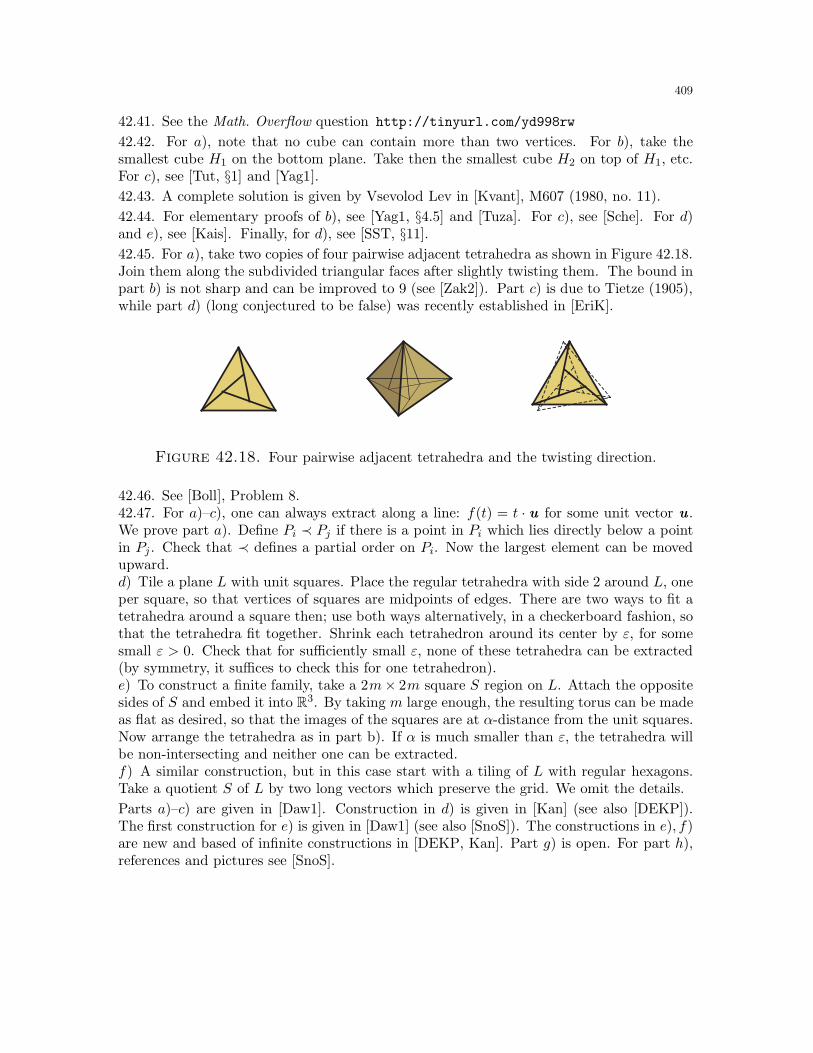
409

42.41. See the Math. Overflow question http://tinyurl.com/yd998rw

42.42. For a), note that no cube can contain more than two vertices. For b), take thesmallest cube H1 on the bottom plane. Take then the smallest cube H2 on top of H1, etc.For c), see [Tut, §1] and [Yag1].

42.43. A complete solution is given by Vsevolod Lev in [Kvant], M607 (1980, no. 11).

42.44. For elementary proofs of b), see [Yag1, §4.5] and [Tuza]. For c), see [Sche]. For d)and e), see [Kais]. Finally, for d), see [SST, §11].

42.45. For a), take two copies of four pairwise adjacent tetrahedra as shown in Figure 42.18.Join them along the subdivided triangular faces after slightly twisting them. The bound inpart b) is not sharp and can be improved to 9 (see [Zak2]). Part c) is due to Tietze (1905),while part d) (long conjectured to be false) was recently established in [EriK].

Figure 42.18. Four pairwise adjacent tetrahedra and the twisting direction.

42.46. See [Boll], Problem 8.42.47. For a)–c), one can always extract along a line: f(t) = t · u for some unit vector u .We prove part a). Define Pi ≺ Pj if there is a point in Pi which lies directly below a pointin Pj . Check that ≺ defines a partial order on Pi. Now the largest element can be movedupward.d) Tile a plane L with unit squares. Place the regular tetrahedra with side 2 around L, oneper square, so that vertices of squares are midpoints of edges. There are two ways to fit atetrahedra around a square then; use both ways alternatively, in a checkerboard fashion, sothat the tetrahedra fit together. Shrink each tetrahedron around its center by ε, for somesmall ε > 0. Check that for sufficiently small ε, none of these tetrahedra can be extracted(by symmetry, it suffices to check this for one tetrahedron).e) To construct a finite family, take a 2m× 2m square S region on L. Attach the oppositesides of S and embed it into R3. By taking m large enough, the resulting torus can be madeas flat as desired, so that the images of the squares are at α-distance from the unit squares.Now arrange the tetrahedra as in part b). If α is much smaller than ε, the tetrahedra willbe non-intersecting and neither one can be extracted.f) A similar construction, but in this case start with a tiling of L with regular hexagons.Take a quotient S of L by two long vectors which preserve the grid. We omit the details.

Parts a)–c) are given in [Daw1]. Construction in d) is given in [Kan] (see also [DEKP]).The first construction for e) is given in [Daw1] (see also [SnoS]). The constructions in e), f)are new and based of infinite constructions in [DEKP, Kan]. Part g) is open. For part h),references and pictures see [SnoS].

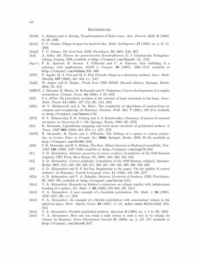
410

References

[AbrK] J. Abrham and A. Kotzig, Transformations of Euler tours, Ann. Discrete Math. 8 (1980),65–69. [398]

[Ada1] C. C. Adams, Tilings of space by knotted tiles, Math. Intelligencer 17 (1995), no. 2, 41–51.[390]

[Ada2] C. C. Adams, The knot book, AMS, Providence, RI, 2004. [240, 397][Adl] A. Adler, Die Theorie der geometrischen Konstruktionen, G. J. Goschensche Verlagshan-

dulung, Leipzig, 1906; available at http://tinyurl.com/2kyaw3 ; (J). [116][Aga+] P. K. Agarwal, B. Aronov, J. O’Rourke and C. A. Schevon, Star unfolding of a

polytope with applications, SIAM J. Comput. 26 (1997), 1689–1713; available athttp://tinyurl.com/62dda4 [358, 406]

[AFF] F. Aguilo, M. A. Fiol and M. L. Fiol, Periodic tilings as a dissection method, Amer. Math.Monthly 107 (2000), 341–352; (). [147]

[AigZ] M. Aigner and G. Ziegler, Proofs from THE BOOK (Second edition), Springer, Berlin,2003. [31, 215]

[AHKN] J. Akiyama, K. Hirata, M. Kobayashi and G. Nakamura, Convex developments of a regulartetrahedron, Comput. Geom. 34 (2006), 2–10; [405]

[Alb] S. I. Al′ber, On periodicity problem in the calculus of large variations in the large, Amer.Math. Transl. 14 (1960), 107–172; (ℜ). [101, 385]

[ABe] M. V. Alekhnovich and A. Ya. Belov, The complexity of algorithms of constructions bycompass and straightedge (in Russian), Fundam. Prikl. Mat. 7 (2001), 597–614; availableat http://tinyurl.com/3dwerb [116]

[AVS] D. V. Alekseevskij, E. B. Vinberg and A. S. Solodovnikov, Geometry of spaces of constantcurvature, in Geometry II, 1–138, Springer, Berlin, 1993; (ℜ). [272]

[Ale] R. Alexander, Lipschitzian mappings and total mean curvature of polyhedral surfaces. I,Trans. AMS 288 (1985), 661–678; (). [271, 272]

[ADO] R. Alexander, H. Dyson and J. O’Rourke, The foldings of a square to convex polyhe-dra, in Lecture Notes in Comput. Sci. 2866, Springer, Berlin, 2003, 38–50; available athttp://tinyurl.com/56c86v [404]

[ABi] S. B. Alexander and R. L. Bishop, The Fary–Milnor theorem in Hadamard manifolds, Proc.AMS 126 (1998), 3427–3436; available at http://tinyurl.com/ytgl78 [240]

[A1] A. D. Alexandrov, Intrinsic geometry of convex surfaces (translation of the 1948 Russianoriginal), CRC Press, Boca Raton, FL, 2005. [101, 262, 334, 358]

[A2] A. D. Alexandrov, Convex polyhedra (translation of the 1950 Russian original), Springer,Berlin, 2005. [215, 248, 256, 262, 271, 300, 321, 328, 334, 369, 396, 402, 404]

[AS] A. D. Aleksandrov and E. P. Sen’kin, Supplement to the paper “On the rigidity of convexsurfaces” (in Russian), Vestnik Leningrad. Univ. 11 (1956), 104–106. [277]

[AZa] A. D. Aleksandrov and V. A. Zalgaller, Intrinsic Geometry of Surfaces, AMS, Providence,RI, 1967; (ℜ); available at http://tinyurl.com/3xvtar [101]

[Ale1] V. A. Alexandrov, Remarks on Sabitov’s conjecture on volume rigidity with infinitesimalbending of a surface, Sib. Math. J. 30 (1989), 678–684; (ℜ). [314]

[Ale2] V. A. Alexandrov, A new example of a bendable polyhedron, Sib. Math. J. 36 (1995),1049–1057; (ℜ), (). [285]

[Ale3] V. A. Alexandrov, An example of a flexible polyhedron with nonconstant volume in thespherical space, Beitr. Algebra Geom. 38 (1997), 11–18; arXiv:math.MG/0111003. [285,314]

[Ale4] V. A. Alexandrov, Flexible polyhedral surfaces, Quantum 9 (1998), no. 1, 4–6; (ℜ). [285][Ale5] V. A. Alexandrov, How one can crush a milk carton in such a way as to enlarge its

volume (in Russian), Soros Educational Journal 51 (2000), no. 2, 121–127; available athttp://tinyurl.com/3acu49 [347]

411

[Ale6] V. A. Alexandrov, Inverse function theorems and their applications to the theory of poly-hedra, to appear in Rev. Math. Math. Phys. [256, 285, 300, 314, 369]

[AleC] V. Alexandrov and R. Connelly, Flexible suspensions with a hexagonal equator; arXiv:

0905.3683. [291][AlmR] F. J. Almgren and I. Rivin, The mean curvature integral is invariant under bending, in The

Epstein birthday schrift, Coventry, UK, 1998, 1–21; arXiv:math.DG/9810183. [272][Alon] N. Alon, Splitting necklaces, Adv. in Math. 63 (1987), 247–253. [38, 379][AloG] N. Alon and E. Gyori, The number of small semispaces of a finite set of points in the plane,

J. Combin. Theory Ser. A 41 (1986), 154–157; (). [396][And+] A. Andrzejak, B. Aronov, S. Har-Peled, R. Seidel and E. Welzl, Results on k-sets and j-

facets via continuous motion, in Proc. 14th Symp. Comp. Geom. (1998), 192–199; availableat http://tinyurl.com/25nqoo8 [228]

[Ani] S. S. Anisov, Convex curves in RPn, Proc. Steklov Inst. Math. 221 (1998), 3–39; availableat http://tinyurl.com/2drfjw4 [378]

[Arn1] V. I. Arnold, Topological invariants of plane curves and caustics, AMS, Providence, RI,1994. [206]

[Arn2] V. I. Arnold, Topological problems in the theory of wave propagation, Russian Math.Surveys 51 (1996), 1–47; (ℜ), (). [94, 396]

[Arn3] V. I. Arnold, Arnold’s problems, Springer, Berlin, 2004; (ℜ). [206, 358, 407][AroO] B. Aronov and J. O’Rourke, Nonoverlap of the star unfolding, Discrete Comput. Geom. 8

(1992), 219–250; (). [358, 406][AroW] B. Aronov and E. Welzl, Identities involving crossings of j-edges, unpublished manuscript

(2004). [228][AtiM] M. F. Atiyah and I. G. Macdonald, Introduction to commutative algebra, Addison-Wesley,

Reading, MA, 1969; (ℜ). [314][Aur] F. Aurenhammer, Voronoi diagrams-a survey of a fundamental geometric data structure,

ACM Comp. Surveys 23 (1991), 345–405; available at http://tinyurl.com/24vkn6q [138][AurK] F. Aurenhammer and R. Klein, Voronoi diagrams, in Handbook of computational geometry,

201–290, North-Holland, Amsterdam, 2000; available at http://tinyurl.com/29y2k3b

[138, 206][BajB] E. G. Bajmoczy and I. Barany, On a common generalization of Borsuk’s and Radon’s

theorem, Acta Math. Acad. Sci. Hungar. 34 (1979), 347–350; (). [377][Bag] F. Bagemihl, On indecomposable polyhedra, Amer. Math. Monthly 55 (1948), 411–413; ().

[388][BVK] I. Ya. Bakel′man, A. L. Verner and B. E. Kantor, Introduction to differential geometry “in

the large” (in Russian), Nauka, Moscow, 1973. [277][Bak] M. J. C. Baker, A spherical Helly-type theorem, Pacific J. Math. 23 (1967), 1–3; available

at http://tinyurl.com/2wq9q5 [377][Bali] M. L. Balinski, On the graph structure of convex polyhedra in n-space. Pac. J. Math. 11

(1961), 431–434; available at http://tinyurl.com/33fbdel [82][Ball] N. H. Ball, On ovals, Amer. Math. Monthly 37 (1930), 348–353; (). [396][Ban1] T. F. Banchoff, Non-rigidity theorems for tight polyhedra, Arch. Math. 21 (1970), 416–423.

[285][Ban2] T. F. Banchoff, Global geometry of polygons. I: The theorem of Fabricius-Bjerre, Proc.

AMS 45 (1974), 237–241; (). [228][BanG] T. F. Banchoff and P. J. Giblin, Global theorems for symmetry sets of smooth curves and

polygons in the plane, Proc. Roy. Soc. Edinburgh 106 (1987), 221–231. [206][Bar] I. Barany, A generalization of Caratheodory’s theorem, Discrete Math. 40 (1982), 141–

152; (). [378][BaFu] I. Barany and K. Fukuda, A case when the union of polytopes is convex, Linear Algebra

Appl. 397 (2005), 381–388; available at http://tinyurl.com/5ohvoo [378]

412

[BKP] I. Barany, M. Katchalski and J. Pach, Helly’s theorem with volumes, Amer. Math.Monthly 91 (1984), 362–365; (). [378]

[BKZ] I. Barany, K. Kuperberg and T. Zamfirescu, Total curvature and spiralling shortest paths,Discrete Comput. Geom. 30 (2003), 167–176; arXiv:math.MG/0301338 [406]

[BarM] I. Barany and J. Matousek, Berge’s theorem, fractional Helly, and art galleries, DiscreteMath. 306 (2006), 2303–2313; available at http://tinyurl.com/254ydrs [377]

[BarV] I. Barany and A. M. Vershik, On the number of convex lattice polytopes, Geom. Funct.Anal. 2 (1992), 381–393; (). [328]

[BDE] G. Barequet, M. Dickerson and D. Eppstein, On triangulating three-dimensional polygons,Comput. Geom. 10 (1998), no. 3, 155–170; available at http://tinyurl.com/23caks5

[387][Bar1] D. W. Barnette, Projections of 3-polytopes, Israel J. Math. 8 (1970), 304–308; (). [387][Bar2] D. W. Barnette, Preassigning the shape of projections of convex polytopes, J. Combin.

Theory Ser. A 42 (1986), 293–295; (). [387][Bar3] D. W. Barnette, A short proof of the d-connectedness of d-polytopes, Discrete Math. 137

(1995), 351–352. [25, 82][Barv] A. Barvinok, A course in convexity, AMS, Providence, RI, 2002. [5, 81, 176, 384][BecB] E. F. Beckenbach and R. Bellman, Inequalities, Springer, Berlin, 1961; (ℜ). [369][Ben] D. Benko, A new approach to Hilbert’s third problem, Amer. Math. Monthly 114 (2007),

665–676; (). [147][Ber1] M. Berger, Geometry I and II (translation of the 1977 French original), Springer, Berlin,

1987. [215, 248, 369][Ber2] M. Berger, Les paquets de cercles, in Differential geometry and topology, 23–64, World Sci.,

River Edge, NJ, 1993. [108][BerE] M. Bern and D. Eppstein, Mesh generation and optimal triangulation, in Comput-

ing in Euclidean geometry, 23–90, World Sci., River Edge, NJ, 1992; available athttp://tinyurl.com/5gg8jw [387, 388]

[BerH] M. W. Bern and B. Hayes, Origami embedding of piecewise-linear two-manifolds, in Proc.8th LATIN (2008), 617–629; (). [406]

[BesE] A. S. Besicovitch and H. G. Eggleston, The total length of the edges of a polyhedron,Quart. J. Math. Oxford Ser. (2) 8 (1957), 172–190. [382]

[Bes1] A. S. Besicovitch, A net to hold a sphere, Math. Gaz. 41 (1957), 106–107; (). [399][Bes2] A. S. Besicovitch, A cage to hold a unit-sphere, in Proc. Sympos. Pure Math., vol. VII,

AMS, Providence, RI, 1963, 19–20. [382][BezB] A. Bezdek and K. Bezdek, When it is possible to translate a convex polyhedron in an other

one? Stud. Sci. Math. Hung. 21 (1986), 337–342. [404][Bez] K. Bezdek, Sphere packings revisited, Europ. J. Comb. 27 (2006), 864–883; available at

http://tinyurl.com/2sxww6 [191][Bieb] L. Bieberbach, Theorie der geometrischen Konstruktionen, Birkhauser, Basel, 1952. [116][Biel] A. Bielecki, Quelques remarques sur la note precedente, Ann. Univ. Mariae Curie-

Sk lodowska. Sect. A. 8 (1954), 101–103. [381][Bin] D. Binger, Polyhedra with unguarded interiors, Int. J. Comput. Geom. Appl. 12 (2002),

173–179; (). [388][Bir] G. D. Birkhoff, Dynamical Systems, AMS, Providence, RI, 1927; (ℜ). [385][Bjo+] A. Bjorner, M. Las Vergnas, B. Sturmfels, N. White and G. M. Ziegler, Oriented matroids,

Cambridge U. Press, Cambridge, 1993. [138]

[Bla1] W. Blaschke, Vorlesungen Uber Differentialgeometrie, Springer, Berlin, 1929; (ℜ). [206,339]

[Bla2] W. Blaschke, Griechische und anschauliche Geometrie, R. Oldenbourg, Munchen, 1953;(ℜ). [248, 256]

[Bla3] W. Blaschke, Kreis und Kugel, de Gruyter, Berlin, 1956; (J). [70, 206]

413

[Ble] D. D. Bleecker, Volume increasing isometric deformations of convex polyhedra, J. Diff.Geom. 43 (1996), 505–526; available at http://tinyurl.com/37tcwh [347, 405]

[BobI] A. I. Bobenko and I. Izmestiev, Alexandrov’s theorem, weighted Delaunay triangulations,and mixed volumes, Ann. Inst. Fourier 58 (2008), 447–505; arXiv:math.DG/0609447.[334]

[BojF] V. Boju and L. Funar, The Math Problems Notebook, Birkhauser, Boston, MA, 2007. [378][Boll] B. Bollobas, The Art of Mathematics: Coffee Time in Memphis, Cambridge U. Press,

Cambridge, UK, 2007. [409][Bolt] V. G. Boltyanskii, Hilbert’s Third Problem, John Wiley, New York, 1978; (J). [5, 147, 157,

390, 392][BolG] V. G. Boltjansky and I. Ts. Gohberg, Results and problems in combinatorial geometry,

Cambridge U. Press, Cambridge, UK, 1985; (J). [31, 378, 379, 396][BMS] V. Boltyanski, H. Martini and P. S. Soltan, Excursions into combinatorial geometry,

Springer, Berlin, 1997. [31][BolS] V. G. Boltjanskii and P. S. Soltan, Combinatorial geometry of various classes of convex

sets (in Russian), Stiinca, Kishinev, 1978. [377, 408][BolY] V. G. Boltyanski and I. M. Yaglom, Convex sets (in Russian), in Encyclopedia of Elementary

Mathematics, vol. V, Fizmatgiz, Moscow, 1966, 192–269; (J). [71][BonF] T. Bonnesen and W. Fenchel, Theory of convex bodies, BCS, Moscow, ID, 1987; (ℜ)[70,

328, 404][Bor] O. Borodin, Joint extension of two theorems of Kotzig on 3-polytopes, Combinatorica 13

(1993), 121–125; (). [383][BorF] E. Boros and Z. Furedi, The number of triangles covering the center of an n-set, Geom.

Dedicata 17 (1984), 69–77; (). [25, 38, 379][BorB] A. V. Borovik and A. S. Borovik, Mirrors and Reflections: The Geometry of Finite and

Affine Reflection Groups, Birkhauser, Boston, MA, 2004. [184][BorM] P. Borwein and W. O. J. Moser, A survey of Sylvester’s problem and its generalizations,

Aeq. Math. 40 (1990), 111–135; available at http://tinyurl.com/63ttwy [25, 378][BouK] M. Boutin and G. Kemper, On reconstructing n-point configurations from the distribution

of distances or areas, Adv. Appl. Math. 32 (2004), 709–735; arXiv:math/0304192 [403][BraW] P. Brass and C. Wenk, On the number of cylinders touching a ball, Geom. Dedicata 81

(2000), 281–284; (). [395][Bre] M. Breen, A Helly-type theorem for intersections of compact connected sets in the plane,

Geom. Dedicata 71 (1998), 111–117; (). [377][Bri1] R. Bricard, Sur une question de geometrie relative aux polyedres, Nouv. Ann. Math. 15

(1896), 331–334; available at http://tinyurl.com/2s4rdp [147, 390][Bri2] R. Bricard, Memoire sur la theorie de l’octaedre articule, J. Math. Pures Appl. 3 (1897),

113–150; English translation is available at http://tinyurl.com/2pa63m [285][Brø] A. Brøndsted, An introduction to convex polytopes, Springer, New York, 1983; (ℜ). [81][BrøM] A. Brøndsted and G. Maxwell, A new proof of the d-connectedness of d-polytopes, Canad.

Math. Bull. 32 (1989), 252–254. [382][Buck] R. C. Buck and E. F. Buck, Equipartition of convex sets, Math. Mag. 22 (1949), 195–

198; (). [37, 379][Bukh] B. Bukh, A point in many triangles, Electron. J. Combin. 13 (2006), no. 1, Note 10, 3 pp.;

available at http://tinyurl.com/376l9h [38][BMN] B. Bukh, J. Matousek and G. Nivasch, Stabbing simplices by points and flats; arXiv:

0804.4464 [38, 379][BBI] D. Burago, Yu. Burago and S. Ivanov, A course in metric geometry, AMS, Providence, RI,

2001; (ℜ). [358][BZ1] Ju. D. Burago and V. A. Zalgaller, Polyhedral embedding of a net (in Russian), Vestnik

Leningrad. Univ. 15 (1960), no. 7, 66–80. [405]

414

[BZ2] Ju. D. Burago and V. A. Zalgaller, Sufficient criteria of convexity J. Math. Sci. 10 (1978),395–435; (ℜ), (). [377]

[BZ3] Yu. D. Burago and V. A. Zalgaller, Geometric inequalities, Springer, Berlin, 1988; (ℜ). [71,398, 404]

[BZ4] Yu. D. Burago and V. A. Zalgaller, Isometric piecewise-linear embeddings of two-dimensional manifolds with a polyhedral metric into R3, St. Petersburg Math. J. 7 (1996),369–385; (ℜ). [347, 387, 405]

[Bus] H. Busemann, The geometry of geodesics, Academic Press, New York, 1955; (ℜ). [248][Caf] L. Caffarelli, The Monge-Ampere equation and optimal transportation, an elementary re-

view, in Lecture Notes in Math. 1813, Springer, Berlin, 2003, 1–10; (). [176][CanR] J. F. Canny and J. H. Reif, New lower bound techniques for robot motion planning prob-

lems, Proc. 28th FOCS (1987), 49–60. [406][Can+] J. Cantarella, J. H. G. Fu, R. Kusner, J. M. Sullivan and N. C. Wrinkle, Criticality for

the Gehring link problem, Geom. Topol. 10 (2006), 2055–2116; arXiv:math.DG/0402212

[240][CanJ] J. Cantarella and H. Johnston, Nontrivial embeddings of polygonal intervals and un-

knots in 3-space, J. Knot Theory Ramifications 7 (1998), 1027–1039; available athttp://tinyurl.com/2f9s2pv [396]

[CKKS] J. Cantarella, G. Kuperberg, R. B. Kusner and J. M. Sullivan, The second hull of a knottedcurve, Amer. J. Math. 125 (2003), 1335–1348; arXiv:math/0204106 [240, 398]

[Car] P. Cartier, Decomposition des polyedres: le point sur le troisieme probleme de Hilbert,Asterisque 133–134 (1986), 261–288; (ℜ); available at http://tinyurl.com/3e4cnb [147]

[Carv] F. J. C. de Carvalho, Characterizing maximally looped closed curves, Amer. Math.Monthly 92 (1985), 202–207; (). [396]

[Cha] G. D. Chakerian, An inequality for closed space curves, Pacific J. Math. 12 (1962), 53–57;available at http://tinyurl.com/37v9yh [398]

[ChaK] G. D. Chakerian and M. S. Klamkin, Minimal covers for closed curves, Math. Mag. 46(1973), 55–61. [240]

[CEG] B. Chazelle, H. Edelsbrunner and L. J. Guibas, The complexity of cutting complexes,Discrete Comput. Geom. 4 (1989), 139–181; (). [407]

[Chen] W. Chen, Counterexamples to Knaster’s conjecture, Topology 37 (1998), 401–405; (). [60][Cher] S. S. Chern, Curves and surfaces in Euclidean space, in Studies in Global Geometry and

Analysis, MAA, 1967, 16–56. [206, 240, 397][CocO] R. Cocan and J. O’Rourke, Polygonal chains cannot lock in 4D, Comput. Geom. 20 (2001),

no. 3, 105–129; arXiv:cs.CG/9908005 [396][CSE] D. Cohen-Steiner and H. Edelsbrunner, Inequalities for the curvature of curves and surfaces,

Found. Comput. Math. 7 (2007), 391–404; available at http://tinyurl.com/2f2tmqg [398,401]

[Cohn] P. M. Cohn, Skew fields, Cambridge U. Press, Cambridge, 1995. [314][CV] S. Cohn-Vossen, Kurzeste Wege und Totalkrummung auf Flachen, Composito Math. 2

(1935), 63–133; (ℜ), avaialable at http://tinyurl.com/3acm4p [248][Con1] R. Connelly, The rigidity of suspensions, J. Differential Geom. 13 (1978), 399–408; see also

An attack on rigidity I, II (1974); (ℜ), available at http://tinyurl.com/3b58yg [401][Con2] R. Connelly, Conjectures and open questions in rigidity, in Proc. ICM Helsinki, Acad. Sci.

Fennica, Helsinki, 1980, 407–414. [285, 291, 314][Con3] R. Connelly, The rigidity of certain cabled frameworks and the second-order rigidity of

arbitrarily triangulated convex surfaces, Adv. in Math. 37 (1980), 272–299; available athttp://tinyurl.com/2fyyjph [402]

[Con4] R. Connelly, Flexing surfaces, in The mathematical Gardner (Edited by D. A. Klarner),79–89, PWS Publishers, Boston, MA, 1981; (ℜ). [285, 291]

[Con5] R. Connelly, Rigidity, in Handbook of Convex Geometry, vol. A, North-Holland, Amster-dam, 1993, 223–271. [215, 253, 262, 293, 300, 302, 306, 402]

415

[Con6] R. Connelly, Comments on generalized Heron polynomials and Robbins’ conjectures,preprint; available at http://tinyurl.com/36zmzy [314, 403]

[CDR] R. Connelly, E. D. Demaine and G. Rote, Straightening polygonal arcs and con-vexifying polygonal cycles, Discrete Comput. Geom. 30 (2003), 205–239; available athttp://tinyurl.com/28uv3ou [228]

[CSW] R. Connelly, I. Sabitov and A. Walz, The bellows conjecture, Beitr. Algebra Geom. 38(1997), 1–10; available at http://tinyurl.com/3ylche [314]

[ConS] R. Connelly and H. Servatius, Higher-order rigidity—what is the proper definition?, Dis-crete Comput. Geom. 11 (1994), 193–200; available at http://tinyurl.com/5tuf7q [306,402]

[CGG] J. H. Conway, M. Goldberg and R. K. Guy, Problem 66-12, SIAM Review 11 (1969), 78–82.[94, 385]

[CRS] J. H. Conway, C. Radin and L. Sadun, On angles whose squared trigonometric functionsare rational, Discrete Comput. Geom. 22 (1999), 321–332; arXiv:math-ph/9812019 [392]

[ConS] J. H. Conway and N. J. A. Sloane, Sphere Packings, Lattices, and Groups (Third edition),Springer, New York, 1999; (ℜ). [191]

[CouR] R. Courant and H. Robbins, What is mathematics?, Oxford U. Press, New York, 1996; (J).[37, 116, 123]

[Cox1] H. S. M. Coxeter, Regular polytopes (Third edition), Dover, New York, 1973. [184, 392,394]

[Cox2] H. S. M. Coxeter, Orthogonal trees, Bull. Inst. Combin. Appl. 3 (1991), 83–91; (). [392][CoxG] H. S. M. Coxeter and S. L. Greitzer, Geometry revisited, McGraw-Hill, New York, 1967; (J).

[385][Crof] H. T. Croft, A net to hold a sphere, J. Lond. Math. Soc. 39 (1964), 1–4; (). [399][CFG] H. T. Croft, K. J. Falconer and R. K. Guy, Unsolved problems in geometry, Springer, New

York, 1991. [94, 380, 407][CroS] H. T. Croft and H. P. F. Swinnerton-Dyer, On the Steinhaus billiard table problem, Proc.

Cambridge Philos. Soc. 59 (1963), 37–41. [385][CroW] H. T. Croft and W. G. Wild, E2152, Amer. Math. Monthly 76 (1969), 1140; (). [384][Crom] P. R. Cromwell, Polyhedra, Cambridge U. Press, Cambridge, UK, 1997. [184, 248, 394][Csa] A. Csaszar, A polyhedron without diagonals, Acta Univ. Szeged. Math. 13 (1949), 140-142.

[408][Cun] H. M. Cundy, Deltahedra, Math. Gaz. 36 (1952), 263–266; (). [394][Daw1] R. Dawson, On removing a ball without disturbing the others, Math. Mag. 57 (1984),

27–30; (). [409][Daw2] R. J. M. Dawson, Monostatic Simplexes, Amer. Math. Monthly 92 (1985), 541–546; ().

[94, 385][Daw3] R. J. M. Dawson, Tilings of the sphere with isosceles triangles, Discrete Comput. Geom. 30

(2003), 467–487; (). [395][DGK] L. Danzer, B. Grunbaum and V. Klee, Helly’s theorem and its relatives, in Convexity, AMS,

Providence, RI, 1963, 101–180; (ℜ). [19, 377][Deb1] H. E. Debrunner, Zerlegungsrelationen zwischen regularen Polyedern des Ed, Arch.

Math. 30 (1978), 656-660. [392][Deb2] H. E. Debrunner, Dissecting orthoschemes into orthoschemes, Geom. Dedicata 33 (1990),

123–152; (). [392][DML] H. E. Debrunner and P. Mani-Levitska, Can you cover your shadows? Discrete Comput.

Geom. 1 (1986), 45–58; available at http://tinyurl.com/2v2rwy [408]

[Dehn] M. Dehn, Uber die Starreit konvexer Polyeder, Math. Ann. 77 (1916), 466–473; (ℜ); avail-able at http://tinyurl.com/35kkkx [300]

[Deho] P Dehornoy, On the rotation distance between binary trees, Adv. Math. 223/4 (2010),1316–1355; arXiv:0901.2557. [387]

416

[DRS] J. A. De Loera, J. Rambau and F. Santos, Triangulations: Structures and Algorithms,Springer, 2008. [138, 387, 388]

[DGOT] E. D. Demaine, B. Gassend, J. O’Rourke and G. T. Toussaint, Polygons flip finitely: flawsand a fix, in Proc. CCCG 2006, 109–112; available at http://tinyurl.com/2sdpt3 [397]

[Dev] M. Develin, Disjoint faces of complementary dimension, Beitr. Algebra Geom. 45 (2004),463–464; available at http://tinyurl.com/2rdvl6 [383]

[Dek] B. V. Dekster, Convex hulls of spatial polygons with a fixed convex projection, Beitr.Algebra Geom. 36 (1995), 123–134; available at http://tinyurl.com/2vbedt [388]

[Den] E. Denne, Alternating quadrisecants of knots, arXiv:math.GT/0510561. [240, 398][DeoK] N. Deo and M. S. Klamkin, Existence of four concurrent normals to a smooth closed curve,

Amer. Math. Monthly 77 (1970), 1083–1084; (). [385][DGPV] D. DeTurck, H. Gluck, D. Pomerleano and D. S. Vick, The four vertex theorem and its

converse, Notices AMS 54 (2007), 192–207; available at http://tinyurl.com/2kwjkn

[206][DiaK] P. Diaconis and J. B. Keller, Fair dice, Amer. Math. Monthly 96 (1989), 337–339; (). [394][Dil] M. B. Dillencourt, Realizability of Delaunay triangulations, Inform. Process. Lett. 33

(1990), no. 6, 283–287; (). [388][Dol] N. P. Dolbilin, Gems of Polytope Theory (in Russian), MCCME, Moscow, 2000; (J). [285][DSS1] N. P. Dolbilin, M. A. Shtan′ko and M. I. Shtogrin, Nonbendability of polyhedral spheres

with even-sided faces, Russian Math. Surveys 51 (1996), 543–544; (ℜ), (). [402][DSS2] N. P. Dolbilin, M. A. Shtan′ko and M. I. Shtogrin, Rigidity of a quadrillage of a torus by

squares, Russian Math. Surveys 54 (1999), 839–840; (ℜ), (). [400][Dup] J. L. Dupont, Scissors congruences, group homology and characteristic classes, World Sci.,

River Edge, NJ, 2001; available at http://tinyurl.com/376ol6 [5, 147][Dvo] A. Dvoretzky, A converse of Helly’s theorem on convex sets, Pacific J. Math. 5 (1955),

345–350; available at http://tinyurl.com/2wjvsv [377][DEKP] A. V. Dyskin, Y. Estrin, A. J. Kanel-Belov and E. Pasternak, Topological interlocking of

platonic solids, Phil. Mag. Letters 83 (2003), 197–203; (). [409][Dys] F. J. Dyson, Continuous functions defined on spheres, Ann. of Math. 54 (1951), 534–536;

(). [60][Eck] J. Eckhoff, Helly, Radon, and Caratheodory type theorems, in Handbook of Convex Geom-

etry, vol. A, 389–448, North-Holland, Amsterdam, 1993. [19][EdeS] M. Edelstein and B. Schwarz, On the length of linked curves, Israel J. Math. 23 (1976),

94–95; (). [240][Edm1] A. L. Edmonds, The geometry of an equifacetal simplex, Mathematika 52 (2005), 31–45;

arXiv:math.MG/0408132 [394][Edm2] A. L. Edmonds, Sommerville’s missing tetrahedra, Discrete Comput. Geom. 37 (2007),

287–296; (). [392][Egg1] H. G. Eggleston, Convexity, Cambridge U. Press, Cambridge, UK, 1958. [71, 379][Egg2] H. G. Eggleston, Figures inscribed in convex sets, Amer. Math. Monthly 65 (1958), 76–80;

(). [380][Emch] A. Emch, Some properties of closed convex curves in a plane, Amer. J. Math. 35 (1913),

407–412; (). [53, 379][EKK] V. A. Emelichev, M. M. Kovalev and M. K. Kravtsov, Polytopes, Graphs, and Optimization,

Cambridge U. Press, New York, 1984; (ℜ). [82, 384][Epp] D. Eppstein, The farthest point Delaunay triangulation minimizes angles, Comput. Geom. 1

(1992), no. 3, 143–148; available at http://tinyurl.com/6fzxer [387]

[ESU] D. Eppstein, J. M. Sullivan and A. Ungor, Tiling space and slabs with acute tetrahedra,Comput. Geom. 27 (2004), 237–255; arXiv:cs.CG/0302027. [387]

[Erd] P. Erdos, Personal reminiscences and remarks on the mathematical work of Tibor Gallai,Combinatorica 2 (1982), 207–212; available at http://tinyurl.com/6fr55a [25]

417

[ErdP] P. Erdos and G. Purdy, Extremal problems in combinatorial geometry, in Handbook ofCombinatorics, Vol. 1, 809–874, Elsevier, Amsterdam, 1995. [25, 377, 378]

[EriK] J. Erickson and S. Kim, Arbitrarily large neighborly families of congruent symmetric convex3-polytopes, in Discrete Geometry: In Honor of W. Kuperberg’s 60th Birthday, Marcel-Dekker, 2003, 267–278; arXiv:math.CO/0106095. [409]

[Eri] F. Eriksson, The law of sines for tetrahedra and n-simplices, Geom. Dedicata 7 (1978),71–80. [408]

[Euc] Euclid, Elements, Books 1-13; available e.g., at http://tinyurl.com/62x9q5 ; (J). [256][Fab] Fr. Fabricius-Bjerre, A proof of a relation between the numbers of singularities of a closed

polygon, J. Geom. 13 (1979), 126–132. [228][Fed] P. J. Federico, Descartes on polyhedra, Springer, Berlin, 1982. [248][FedP] M. Fedorchuk and I. Pak, Rigidity and polynomial invariants of convex polytopes, Duke

Math. J. 129 (2005), 371-404; available at http://tinyurl.com/3xvj96 [288, 291, 300,401, 402, 403]

[Fej1] L. Fejes Toth, E895, Amer. Math. Monthly 57 (1950), 419–420; (). [382][Fej2] L. Fejes Toth, Lagerungen in der Ebene, auf der Kugel und im Raum, Springer, Berlin,

1953; (J). [71, 184, 191][Fenn] R. Fenn, The table theorem, Bull. London Math. Soc. 2 (1970), 73–76; (). [381][FenR] R. Fenn and C. Rourke, Klyachko’s methods and the solution of equations over torsion-free

groups, L’Ens. Math. 42 (1996), 49–74; available at http://tinyurl.com/374e58 [384]

[Fie] M. Fiedler, Uber qualitative Winkeleigenschaften der Simplexe Czechoslovak Math. J. 7(1957), 463–478; available at http://tinyurl.com/6pc3uj [392]

[FSW] H. Fleischner, G. Sabidussi and E. Wenger, Transforming Eulerian trails, DiscreteMath. 109 (1992), 103–116; (). [398]

[Fle] T. M. Flett, Ampere and the horizontal chord theorem, Bull. Inst. Math. Appl. 11 (1975),no. 1-2, 34. [38]

[Flo] E. E. Floyd, Real-valued mappings of spheres, Proc. AMS 6 (1955), 957–959; (). [60][For] R. Forman, A user’s guide to discrete Morse theory, Sem. Lothar. Combin. 48 (2002),

Art. B48c, 35 pp.; available at http://tinyurl.com/2o9zhu [82][Fox] R. H. Fox, A quick trip through knot theory, in Topology of 3-manifolds and related topics,

120–167, Prentice-Hall, Englewood Cliffs, NJ, 1962; (ℜ). [397][Fri] E. J. Friedman, Finding a simple polytope from its graph in polynomial time, Discrete

Comput. Geom. 41 (2009), 249–256; available at http://tinyurl.com/5om26t [77][FucF] D. Fuchs and E. Fuchs, Closed geodesics on regular polyhedra, Mosc. Math. J. 7 (2007),

265–279. [386][FucT] D. Fuchs and S. Tabachnikov, Mathematical Omnibus. Thirty Lectures on Classic Mathe-

matics, draft of a monograph; available at http://tinyurl.com/2u2c7v [285][Gal] G. Galperin, Convex polyhedra without simple closed geodesics, Regular and Chaotic Dy-

namics 8 (2003), 45–58; (ℜ); available at http://tinyurl.com/3xy8pv [101][Gal+] J. Galtier, F. Hurtado, M. Noy, S. Perennes and J. Urrutia, Simultaneous edge flipping

in triangulations, Internat. J. Comput. Geom. Appl. 13 (2003), 113–133; available athttp://tinyurl.com/plazz8 [387]

[Gar] R. J. Gardner, The Brunn–Minkowski inequality, Bull. AMS 39 (2002), 355–405; availableat http://tinyurl.com/2k8thm [71]

[GarM] R. J. Gardner and P. McMullen, On Hammer’s X-ray problem, J. London Math. Soc. 21(1980), 171–175; (). [381]

[GKZ] I. M. Gelfand, M. M. Kapranov and A. V. Zelevinsky, Discriminants, resultants, and mul-tidimensional determinants, Birkhauser, Boston, MA, 1994. [82, 138]

[Ger] M. L. Gerver, Width of polygons (in Russian), Matemat. Prosv. 2 (1999), 173–191; (J).[381]

[Gla] L. Glass, A combinatorial analog of the Poincare index theorem, J. Combin. Theory Ser.B 15 (1973), 264–268. [399, 400]

418

[Glaz] A. Glazyrin, Lower bounds for the simplexity of the d-cube, to appear in Discrete Math.[388]

[Gle] A. M. Gleason, Angle trisection, the heptagon, and the triskaidecagon, Amer. Math.Monthly 95 (1988), 185–194, 911; (). [387]

[Glu] H. Gluck, Almost all simply connected closed surfaces are rigid, in Lecture Notes inMath. 438, Springer, Berlin, 1975, 225–239; (ℜ), (). [291]

[Gol1] M. Goldberg, Polyhedral linkages, Nat. Math. Mag. 16 (1942), 323–332; (). [123][Gol2] M. Goldberg, Tubular linkages, J. Math. Phys. MIT 26 (1947), 10–21. [285][Gol3] M. Goldberg, Three infinite families of tetrahedral space-fillers, J. Combin. Theory

Ser. A 16 (1974), 348–354; (). [392][Gol4] M. Goldberg, Unstable polyhedral structures, Math. Mag. 51 (1978), 165–170; available at

http://tinyurl.com/6funls [306][Gol5] M. Goldberg, On the space-filling heptahedra, Geom. Dedicata 7 (1978), 175–184; (). [391][GooT] I. J. Good and T. Teichmann, E1923, Amer. Math. Monthly 75 (1968), 194–195; (). [408][GPY] J. E. Goodman, J. Pach and C.-K. Yap, Mountain climbing, ladder moving, and the ring-

width of a polygon, Amer. Math. Monthly 96 (1989), 494–510; (). [53, 381][Gor] I. I. Gordon, Generalization of Kakutani’s theorem on continuous functions given on a

sphere (in Russian), Uspehi Mat. Nauk 10 (1955), no. 1, 97–99. [60][GGT] S. Gortler, C. Gotsman and D. Thurston, One-forms on meshes and applications to 3D

mesh parametrization, Comput. Aided Geom. Design 23 (2006), no. 2, 83–112; available athttp://tinyurl.com/2rbe86 [399]

[GouN] I. P. Goulden and A. Nica, A direct bijection for the Harer-Zagier formula, J. Combin.Theory Ser. A 111 (2005), 224–238; (). [404]

[Gray] A. Gray, Tubes (Second edition), Birkhauser, Basel, 2004; (ℜ). [248][Gri] H. B. Griffiths, The topology of square pegs in round holes, Proc. London Math. Soc. 62

(1991), 647–672; (). [53, 380][GriH] P. Gritzmann and A. Hufnagel, On the algorithmic complexity of Minkowski’s reconstruc-

tion theorem, J. London Math. Soc. 59 (1999), 1081–1100; (). [328][GriK] P. Gritzmann and V. Klee, On the complexity of some basic problems in computational

convexity. II. Volume and mixed volumes, in Polytopes: abstract, convex and computational,Kluwer, Dordrecht, 1994, 373–466; available at http://tinyurl.com/3xeyyh [369]

[GriL] P. Gritzmann and M. Lassak, Estimates for the minimal width of polytopes in-scribed in convex bodies, Discrete Comput. Geom. 4 (1989), 627–635; available athttp://tinyurl.com/65uycm [408]

[Gro] H. Groemer, Stability of geometric inequalities, in Handbook of convex geometry, Vol. A,125–150, North-Holland, Amsterdam, 1993. [328]

[Grub] P. M. Gruber, Convex and discrete geometry, Springer, Berlin, 2007. [5, 70, 71, 108, 168,328, 381, 399, 404]

[Gru1] B. Grunbaum, A simple proof of a theorem of Motzkin, Indag. Math. 26 (1964), 382–384.[383]

[Gru2] B. Grunbaum, Arrangements and spreads, AMS, Providence, RI, 1972. [37][Gru3] B. Grunbaum, No-net polyhedra, Geombinatorics 11 (2002), no. 4, 111–114; available at

http://tinyurl.com/6f6849 [406][Gru4] B. Grunbaum, Convex Polytopes (Second edition), Springer, Berlin, 2003. [81, 108, 117,

248, 386, 400][Gru5] B. Grunbaum, Graphs of polyhedra; polyhedra as graphs, Discrete Math. 307 (2007),

445–463; available at http://tinyurl.com/6s99oc [108][GMS] B. Grunbaum, P. Mani-Levitska and G. C. Shephard, Tiling three-dimensional space with

polyhedral tiles of a given isomorphism type, J. London Math. Soc. 29 (1984), 181–191; ().[387]

[GM1] B. Grunbaum and T. S. Motzkin, Longest simple paths in polyhedral graphs, J. LondonMath. Soc. 37 (1962), 152–160. [383]

419

[GM2] B. Grunbaum and T. S. Motzkin, The number of hexagons and the simplicity ofgeodesics on certain polyhedra, Canad. J. Math. 15 (1963), 744–751; available athttp://tinyurl.com/6xu73m [383]

[Gug1] H. W. Guggenheimer, Differential geometry, McGraw-Hill, New York, 1963. [206][Gug2] H. Guggenheimer, Finite sets on curves and surfaces, Israel J. Math. 3 (1965), 104–112; ().

[53, 228, 381][Gug3] H. Guggenheimer, Research problems: Does there exist a “four normals triangle”? Amer.

Math. Monthly 77 (1970), 177–179; (). [384][Gug4] H. Guggenheimer, On the converse Helly theorem, Amer. Math. Monthly 78 (1971), 278–

279; (). [377][Gul] R. Gulliver, Total curvature of graphs in space, Pure Appl. Math. Quarterly 3 (2007),

773–783; avialable at http://tinyurl.com/2sn2ja [398][Hada] J. Hadamard, Lecons de geometrie II. Geometrie dans l’espace (reprint of the eighth edi-

tion), Sceaux, 1988; (J). [179, 215, 369, 403][Had1] H. Hadwiger, Vorlesungen uber Inhalt, Oberflache und Isoperimetrie, Springer, Berlin,

1957; (ℜ). [70][Had2] H. Hadwiger, Homothetieinvariante und additive Polyederfunktionen, Arch. Math. 25

(1974), 203–205; (). [157][HDK] H. Hadwiger, H. Debrunner and V. Klee, Combinatorial Geometry in the Plane, Holt,

Rinehart and Winston, New York, 1964; (ℜ). [19, 31, 378][HadG] H. Hadwiger and P. Glur, Zerlegungsgleichheit ebener Polygone, Elem. Math. 6 (1951),

97–106; available at http://tinyurl.com/2mfwo4 [390][HLM] H. Hadwiger, D. G. Larman and P. Mani, Hyperrhombs inscribed to convex bodies, J.

Combin. Theory Ser. B 24 (1978), 290–293; (). [53, 380, 381][HajW] M. Hajja and P. Walker, Equifacial tetrahedra, Internat. J. Math. Ed. Sci. Tech. 32 (2001),

501–508; (). [407][Hal1] B. Halpern, The kernel of a starshaped subset of the plane, Proc. AMS 23 (1969), 692–

696; (). [377][Hal2] B. Halpern, On the immersion of an n-dimensional manifold in n+1-dimensional Euclidean

space. Proc. AMS 30 (1971), 181–184; (). [377][Hal3] B. Halpern, Double normals and tangent normals for polygons, Proc. AMS 51 (1975),

434–437; (). [396][Hal4] B. Halpern, An inequality for double tangents, Proc. AMS 76 (1979), 133–139; (). [396][Hau] O. Haupt, Zur Verallgemeinerung des Zweischeitelsatzes bei ebenen Kurven, Arch. Math. 11

(1960), 294–297; (). [206][HMS] T. Hausel, E. Makai, and A. Szucs, Inscribing cubes and covering by rhombic dodecahe-

dra via equivariant topology, Mathematika 47 (2000), 371–397; arXiv:math.MG/9906066.[381]

[Heil] E. Heil, Trefoil knots with tritangent planes, Beitrage Algebra Geom. 45 (2004), 527–530;available at http://tinyurl.com/3adcs7 [396]

[HenP] A. Henriques and I. Pak, Volume-preserving PL-maps between polyhedra, preprint; avail-able at http://tinyurl.com/3x25su [176]

[Hep1] A. Heppes, A double-tipping tetrahedron, SIAM Review 9 (1967), 599–600; (). [385][Hep2] A. Heppes, Covering a planar domain with sets of small diameter, Period. Math. Hungar. 53

(2006), 157–168; (). [379][HerR] E. Hertel and C. Richter, Squaring the circle by dissection, Beit. Algebra Geom. 44 (2003),

47–55; available at http://tinyurl.com/34n269 [158][Hil] D. Hilbert, Foundations of geometry, Open Court, LaSalle, Ill., 1971; (ℜ). [116][HilC] D. Hilbert and S. Cohn–Vossen, Geometry and the imagination, Chelsea, New York,

1952; (J). [25, 123][HocR] R. Hochberg and M. Reid, Tiling with notched cubes, Discrete Math. 214 (2000), 255–261;

available at http://tinyurl.com/6jmp6d [390]

420

[Hop1] H. Hopf, Uber die Sehnen ebener Kontinuen und die Schleifen geschlossener Wege, Com-ment. Math. Helv. 9 (1936), 303–319; (ℜ), available at http://tinyurl.com/343gta [38]

[Hop2] H. Hopf, Differential Geometry in the Large, Lecture Notes in Math. 1000, Springer, Berlin,1983. [147, 248]

[Hor] L. Hormander, Notions of convexity, Birkhauser, Boston, MA, 1994. [70][Horn] R. A. Horn, On Fenchel’s theorem, Amer. Math. Monthly 78 (1971), 380–381; (). [240][Hun] N. Hungerbuhler, A short elementary proof of the Mohr–Mascheroni theorem, Amer. Math.

Monthly 101 (1994), 784–787; available at http://tinyurl.com/2uub8j [116][HNU] F. Hurtado, M. Noy and J. Urrutia, Flipping edges in triangulations, Discrete Comput.

Geom. 22 (1999), 333–346; available at http://tinyurl.com/5m2ohq [387][IKS] I. Ivanova-Karatopraklieva and I. Kh. Sabitov, Bending of surfaces. II, J. Math. Sci. 74

(1995), 997–1043. [262, 306, 402][Izm] I. Izmestiev, On the hull numbers of torus links, J. Knot Theory Ramifications 15 (2006),

589–600; arXiv:math.GT/0412139. [398][Izm] I. Izmestiev, A variational proof of Alexandrov’s convex cap theorem; arXiv:

math/0703169. [334][IzmS] I. Izmestiev and J.-M. Schlenker, On the infinitesimal rigidity of polyhedra with vertices in

convex position, to appear in Pacific J. Math; arXiv:arXiv:0711.1981. [169, 393][Jac] S. B. Jackson, Vertices for plane curves, Bull. AMS 50 (1944), 564–478; available at

http://tinyurl.com/2psyqn [206, 380][Jer] R. P. Jerrard, Inscribed squares in plane curves, Trans. AMS 98 (1961), 234–241; (). [53][Jes1] B. Jessen, On equivalence of aggregates of regular polyhedra (in Danish), Mat. Tidsskr. B.

(1946), 145–148. [392][Jes2] B. Jessen, Orthogonal icosahedra, Nordisk Mat. Tidskr. 15 (1967), 90–96. [392, 394][JocP] W. Jockusch and N. Prabhu, Cutting a polytope, Geom. Dedicata 54 (1995), 307–312.

[408][Joh] N. W. Johnson, Convex polyhedra with regular faces, Canad. J. Math. 18 (1966), 169–200.

[184][JucM] E. Jucovic and J. W. Moon, The maximum diameter of a convex polyhedron, Math. Mag. 38

(1965), 31–32. [383]

[Kag1] V. F. Kagan, Uber die Transformation der Polyeder, Math. Ann. 57 (1903), 421–424;available at http://tinyurl.com/396r64 [147]

[Kag2] V. F. Kagan, Foundations of geometry I, II (in Russian), GTI, Moscow, 1949, 1956. [116][Kah] W. Kahan, What has the volume of a tetrahedron to do with computer programming

languages?, UC Berkeley preprint; available at http://tinyurl.com/3amrpg [408][KahK] J. Kahn and G. Kalai, A counterexample to Borsuk’s conjecture, Bull. AMS 29 (1993),

60–62; arXiv:math.MG/9307229. [26, 31][Kaib] V. Kaibel, Reconstructing a simple polytope from its graph, in Combinatorial Optimization,

Springer, New York, 2002, 105–118; arXiv:math/0202103. [77][Kais] H. Kaiser, Perfekte Dreieckzerlegungen, Elem. Math. 46 (1991), 106–111; available at

http://tinyurl.com/3c887y [409][Kake] S. Kakeya, On the inscribed rectangles of a closed curvex curve, Tohoku Math. J. 9 (1916),

163–166. [380][Kaku] S. Kakutani, A proof that there exists a circumscribing cube around any bounded closed

convex set in R3, Ann. of Math. 43 (1942), 739–741; (). [60][Kal1] G. Kalai, A simple way to tell a simple polytope from its graph, J. Combin. Theory,

Ser. A 49 (1988), 381–383; (). [82][Kal2] G. Kalai, Results and Problems around Borsuk’s Conjecture, a talk at PIMS, July 19, 2002;

available at http://tinyurl.com/2vlrul [31][Kall] M. Kallay, Indecomposable polytopes, Israel J. Math. 41 (1982), 235–243; (). [404][Kan] A. Kanel, The story of one olympiad problem (in Russian), Matemat. Prosv. 5 (2001),

207–208; (J). [409]

421

[KM1] M. Kapovich and J. J. Millson, On the moduli space of polygons in the Euclidean plane,J. Diff. Geom. 42 (1995), 430–464; available at http://tinyurl.com/2d2uaj [228]

[KM2] M. Kapovich and J. J. Millson, Moduli spaces of linkages and arrangements, in Ad-vances in geometry, Birkhauser, Boston, MA, 1999, 237–270; available electronically athttp://tinyurl.com/2rb44h [123]

[KM3] M. Kapovich and J. J. Millson, On the moduli space of a spherical polygonal linkage,Canad. Math. Bull. 42 (1999), 307–320; available at http://tinyurl.com/2ka4bz [387]

[KM4] M. Kapovich and J. J. Millson, Universality theorems for configuration spaces of planarlinkages, Topology 41 (2002), 1051–1107; arXiv:math.AG/9803150. [123]

[Kara] R. N. Karasev, On a conjecture of A. Bezdek, Discrete Comput. Geom. 27 (2002), 419–439; (). [378]

[Karc] H. Karcher, Remarks on polyhedra with given dihedral angles, Comm. Pure Appl. Math. 21(1968), 169–174; (). [400]

[KarB] Y. Karshon and C. Bjorndahl, Revisiting Tietze-Nakajima - local and global convexity formaps; arXiv:math/0701745. [138]

[KasS] B. S. Kashin and S. J. Szarek, The Knaster problem and the geometry of high-dimensional cubes, C. R. Math. Acad. Sci. Paris 336 (2003), no. 11, 931–936; available athttp://tinyurl.com/2by5ub [60]

[Kel] T. Keleti, The mountain climbers’ problem, Proc. AMS 117 (1993), 89–97; available athttp://tinyurl.com/25huj25 [53, 381]

[Kem] A. B. Kempe, How to draw a straight line; a lecture on linkages, Macmillan and Co.,London, UK, 1877; available at http://tinyurl.com/2j8jkw [123]

[KenK] C. Kenyon and R. Kenyon, How to take short cuts, Discrete Comput. Geom. 8 (1992),251–264; available at http://tinyurl.com/2jckaz [407]

[Ker] R. B. Kershner, On paving the plane, Amer. Math. Monthly 75 (1968), 839-844; (). [391][King] H. C. King, Planar linkages and algebraic sets, in Proc. 6th Gokova Geometry-Topology

Conf., Turkish J. Math. 23 (1999), 33–56; arXiv:math.AG/9807023. [123][Kis] A. P. Kiselev, Kiselev’s Geometry. Book II. Stereometry (adapted from Russian by A.

Givental), Sumizdat, 2008; (J). [393][Kla] D. A. Klain, The Minkowski problem for polytopes, Adv. Math. 185 (2004), 270–288;

available at http://tinyurl.com/2mhrfh [328][KlaT] M. S. Klamkin and G. A. Tsintsifas, The Circumradius-Inradius Inequality for a Simplex

Math. Mag. 52 (1979), 20–22; (). [408][Klee] V. Klee, Some characterizations of convex polyhedra. Acta Math. 102 (1959), 79–107; ().

[407][KleR] V. Klee and J. R. Reay, A surprising but easily proved geometric decomposition theorem,

Math. Mag. 71 (1998), 3–11; (). [158][KleW] V. L. Klee and S. Wagon, Old and new unsolved problems in plane geometry and number

theory, MAA, Washington, DC, 1991. [53, 94, 381][Kli] W. Klingenberg, Lectures on closed geodesics, Springer, Berlin, 1978; (ℜ). [101][Koe] W. Koenen, Characterizing the circle, Amer. Math. Monthly 78 (1971), 993–996; (). [380][KonP] M. Konvalinka and I. Pak, Geometry and complexity of O’Hara’s algorithm, Adv. Applied

Math. 42 (2009), 157–175; arXiv:0710.1459. [391][KosT] G. Kos and J. Torocsik, Convex disks can cover their shadow, Discrete Comput. Geom. 5

(1990), 529–531; available at http://tinyurl.com/2jrtwz [408][Kos] A. N. Kostovskij, Geometrical constructions using compasses only, Pergamon Press, Oxford,

1961; (J). [116][Kor1] I. G. Korepanov, Multidimensional analogues of geometric s ↔ t duality, Theor. Math.

Phys. 124 (2000), 999–1005; (ℜ), arXiv:solv-int/9911008. [401][Kor2] I. G. Korepanov, Invariants of PL manifolds from metrized simplicial complexes, J. Non-

linear Math. Phys. 8 (2001), 196–210; arXiv:math/0009225. [401]

422

[KorP] M. Korn and I. Pak, Tilings of rectangle with T-tetrominoes, Theor. Comp. Sci. 319 (2004),3–27; available at http://tinyurl.com/323wry [300]

[Kra] H. Kramer, Hyperparallelograms inscribed to convex bodies, Mathematica (Cluj) 22 (1980),no. 1, 67–70. [53, 380]

[Kri] M. Krızek, There is no face-to-face partition of R5 into acute simplices, Discrete Comput.Geom. 36 (2006), 381–390. [387]

[KroK] E. H. Kronheimer and P. B. Kronheimer, The tripos problem, J. London Math. Soc. 24(1981), 182–192. [381]

[Kry] D. A. Kryzhanovskiı, Isoperimeters (in Russian), Fizmatgiz, Moscow, 1959. [70][Kuh] W. Kuhnel, Tight polyhedral submanifolds and tight triangulations, Lecture Notes in

Math. vol1612, Springer, Berlin, 1995; (). [285, 383, 401][Kui] N. H. Kuiper, Double normals of convex bodies, Israel J. Math. 2 (1964), 71–80; (). [385][Kup1] G. Kuperberg, Quadrisecants of knots and links, J. Knot Theory Ramifications 3 (1994),

41–50; arXiv:math.GT/9712205. [398][Kup2] G. Kuperberg, A volume-preserving counterexample to the Seifert conjecture, Comment.

Math. Helv. 71 (1996), 70–97; arXiv:math.DS/9504230. [176][KupS] G. Kuperberg and O. Schramm, Average kissing numbers for non-congruent sphere pack-

ings, Math. Res. Lett. 1 (1994), 339–344; arXiv:math/9405218. [395][Kvant] Kvant Magazine (in Russian), years 1970–2003; (J). [377, 378, 379, 381, 383, 394, 395, 400,

403, 409][LM] J. C. Lagarias and D. Moews, Polytopes that fill Rn and scissors congruence, Discrete

Comput. Geom. 13 (1995), 573–583; and addendum 14 (1995), 359–360; available athttp://tinyurl.com/2qpkkf and http://tinyurl.com/3cgrku [158, 391]

[LR] J. C. Lagarias and T. J. Richardson, Convexity and the average curvature of plane curves,Geom. Dedicata 67 (1997), 1–30; available at http://tinyurl.com/2v9lxd [398]

[Lak] I. Lakatos, Proofs and refutations, Cambridge U. Press, Cambridge, UK, 1976; (ℜ). [248][Lam] T. Lambert, The delaunay triangulation maximizes the mean inradius, in Proc. 6th CCCG

(1994), 201–206; available at http://tinyurl.com/5oce98 [387][Lan] S. Lang, Introduction to algebraic geometry, Addison-Wesley, Reading, MA, 1972. [365][Lang] R. J. Lang, Origami design secrets, A. K. Peters, Natick, MA, 2003. [358, 406][Lass] B. Lass, Demonstration combinatoire de la formule de Harer–Zagier, C. R. Acad. Sci. Paris

Ser. I Math. 333 (2001), 155–160; available at http://tinyurl.com/6phpk7 [404][Leb1] H. Lebesgue, Sur l’equivalence des polyedres..., Ann. Soc. Polon. Math. 17 (1939), 193–226.

[392][Leb2] H. Lebesgue, Lecons sur les Constructions Geometriques, Gauthier-Villars, Paris, 1950.

[116][Leb3] H. Lebesgue, Octaedres articules de Bricard, Enseignement Math. 13 (1967), 175–185;

available at http://tinyurl.com/78ypk3 [285][Lee] J. Leech, Some properties of the isosceles tetrahedron, Math. Gaz. 34 (1950), 269–271; ().

[407][Leib] A. S. Leibin, On the deformability of convex surfaces with a boundary (in Russian), Uspehi

Mat. Nauk 5 (1950), 149–159. [339][Leic] K. Leichtweiss, Konvexe Mengen, Springer, Berlin, 1980; (ℜ). [377][LenW] W. J. Lenhart and S. H. Whitesides, Reconfiguring closed polygonal chains, Discrete Com-

put. Geom. 13 (1995), 123–140; available at http://tinyurl.com/33tbzc [228][Len] N. J. Lennes, Theorems on the simple finite polygon and polyhedron, Amer. J. Math. 33

(1911), 37–62; (). [388][LerW] G. Lerman and J. T. Whitehouse, On d-dimensional d-semimetrics and simplex-type in-

equalities for high-dimensional sine functions; arXiv:0805.1430. [408][Lic] W. B. R. Lickorish, Simplicial moves on complexes and manifolds, in Geom. Topol. Monogr.,

vol. 2, 299–320, Coventry, UK, 1999; arXiv:math.GT/9911256. [168]

423

[Lin] J. Linhart, Uber die Kantenlangensumme von Dreieckspolyedern, Monatsh. Math. 83(1977), 25–36; available at http://tinyurl.com/2khfsh [382]

[Liv] G. R. Livesay, On a theorem of F. J. Dyson, Ann. of Math. 59 (1954), 227–229; (). [381][Lov] L. Lovasz, On the number of halving lines, Ann. Univ. Sci. Budapest. Eotvos Sect. Math. 14

(1971), 107–108. [228][LovP] L. Lovasz and M. D.Plummer, Matching Theory, AMS Chelsea, 2009; (ℜ). [384][LudR] M. Ludwig and M. Reitzner, Elementary moves on triangulations, Discrete Comput.

Geom. 35 (2006), 527–536; arXiv:math.MG/0506564. [168][Luo] F. Luo, Rigidity of polyhedral surfaces, arXiv:math.GT/0612714. [402][Lyu] L. A. Lyusternik, Convex figures and polyhedra, Dover, New York, 1963; (ℜ). [38, 215, 328,

379][Mae1] H. Maehara, Acute triangulations of polygons, Europ. J. Comb. 23 (2002), 45–55; (). [387][Mae2] H. Maehara, The problem of thirteen spheres—a proof for undergraduates, Europ. J. Com-

bin. 28 (2007), 1770–1778; (). [191][Mak1] V. V. Makeev, Inscribed simplices of a convex body, J. Math. Sci. 72 (1994), 3189–3190;

(ℜ), (). [381][Mak2] V. V. Makeev, On quadrangles inscribed in a closed curve and the vertices of a curve,

J. Math. Sci. 131 (2005), no. 1, 5395–5400; (ℜ), (). [380][Man] Yu. I. Manin, On solvability of ruler and compass construction problems (in Russian), in

Encyclopedia of Elementary Mathematics, vol. IV, 205–228, Fizmatgiz, Moscow, 1963; (J).[116]

[Mar] G. E. Martin, Geometric constructions, Springer, New York, 1998. [116][MarW] H. Martini and W. Wenzel, Simplices with congruent k-faces, J. Geom. 77 (2003), 136–139;

(). [394][Mat1] J. Matousek, Lectures on Discrete Geometry, Springer, New York, 2002. [19, 25, 70, 396][Mat2] J. Matousek, Using the Borsuk–Ulam theorem, Springer, Heidelberg, 2003. [31, 38][Mats] H. Matsumura, Commutative ring theory, Cambridge U. Press, Cambridge, 1986. [314][MazM] R. Mazzeo and G. Montcouquiol, Infinitesimal rigidity of cone-manifolds and the Stoker

problem for hyperbolic and Euclidean polyhedra; arXiv:0908.2981. [256][McM1] P. McMullen, Representations of polytopes and polyhedral sets, Geom. Dedicata 2 (1973),

83–99; (). [328, 404][McM2] P. McMullen, Valuations and dissections, in Handbook of convex geometry, 933–988, North-

Holland, Amsterdam, 1993. [168][McS] P. McMullen and E. Schulte, Abstract regular polytopes, Cambridge U. Press, Cambridge,

UK, 2002. [184, 394][Mel] H. Melissen, Loosest circle coverings of an equilateral triangle, Math. Mag. 70 (1997),

118–124; (). [379][Mey] W. Meyer, Indecomposable polytopes, Trans. AMS 190 (1974), 77–86; (). [404][Mey1] M. D. Meyerson, Equilateral triangles and continuous curves, Fund. Math. 110 (1980), 1–9;

available at http://tinyurl.com/2pvbwn [380][Mey2] M. D. Meyerson, Convexity and the table theorem, Pacific J. Math. 97 (1981), 167–169;

available at http://tinyurl.com/2jsj3l [381][Mey3] M. D. Meyerson, Balancing acts, Topology Proc. 6 (1981), 59–75. [53, 380][MeyA] M. D. Meyerson and M. D. Asic, 6385, Amer. Math. Monthly 90 (1983), 651. [380][Mi1] A. D. Milka, On a conjecture of Stoker (in Russian), Ukrainian Geom. Sb. 9 (1970), 85–86.

[-][Mi2] A. D. Milka, The isoperimetry of polygons on the sphere (in Russian), Ukrainian Geom.

Sb. 10 (1971), 49–50. [272][Mi3] A. D. Milka, What is geometry “in the large”? (in Russian), Znanie, Moscow, 1986. [256,

272, 328][Mi4] A. D. Milka, Unique determination of convex surfaces in a pseudo-Riemannian spherical

space. I, J. Soviet Math. 51 (1990), 2273–2276; (ℜ). [262]

424

[Mi5] A. D. Milka, Linear bendings of regular convex polyhedra (in Russian), Mat. Fiz. Anal.Geom. 1 (1994), 116–130. [347, 405]

[Mi6] A. D. Milka, Uniqueness theorems for spacelike convex polyhedra in a pseudo-Euclideanspace (in Russian), Mat. Fiz. Anal. Geom. 2 (1995), 232–249. [262]

[Mill] E. N. Miller, Icosahedra constructed from congruent triangles, Discrete Comput. Geom. 24(2000), 437–451; available at http://tinyurl.com/2lq5qu [394]

[MilP] E. Miller and I. Pak, Metric combinatorics of convex polyhedra: Cut loci and nonoverlap-ping unfoldings, Discrete Comput. Geom. 39 (2008), 339–388; arXiv:math.MG/0312253.[352, 358, 406]

[MilS] E. Miller and B. Sturmfels, Combinatorial commutative algebra, Springer, New York, 2005.[5]

[Mil1] J. W. Milnor, On the total curvature of knots, Ann. of Math. 52 (1950), 248–257; (). [240][Mil2] J. Milnor, The Schlafli differential equality, in Collected Papers, Vol. 1, Geometry, 281–295,

Publish or Perish, Houston, TX, 1994. [272][Min] H. Minkowski, Allegemeine Lehrsatze uber die konvexen Polyeder, see Gesammelte Ab-

handlungen, vol. II (1897), 103–121; (ℜ), available at http://tinyurl.com/33y28j [70,328]

[MMP] J. S. B. Mitchell, D. M. Mount and C. H. Papadimitriou, The discrete geodesic problem,SIAM J. Comp. 16 (1987), 647–668; (ℜ), available at http://tinyurl.com/2prkzg [358]

[MlaO] I. Mladenov and J. Oprea, The mylar balloon revisited, Amer. Math. Monthly 110 (2003),761–784; (). [405]

[Mnev] N. Mnev, The universality theorems..., in Lecture Notes in Math. 1346, Springer, Berlin,1988, 527–543; (). [117]

[Mon1] P. Monsky, On dividing a square into triangles, Amer. Math. Monthly 77 (1970), 161–164; (). [402]

[Mon2] P. Monsky, A conjecture of Stein on plane dissections, Math. Z. 205 (1990), 583–592;available at http://tinyurl.com/6463dx [402]

[Mor] H. R. Morton, Trefoil knots without tritangent planes, Bull. London Math. Soc. 23 (1991),78–80; (). [396]

[Mot] T. S. Motzkin, The evenness of the number of edges of a convex polyhedron, Proc. Nat.Acad. Sci. USA 52 (1964), 44–45; available at http://tinyurl.com/2q9p9t [383]

[MucP] R. Muchnik and I. Pak, On tilings by ribbon tetrominoes, J. Combin. Theory Ser. A 88(1999), 188–193; available at http://tinyurl.com/3aubdc [393]

[Mul] C. Muller, Equidecomposability of polyhedra with reference to crystallographic groups,Discrete Comput. Geom. 3 (1988), 383–389; available at http://tinyurl.com/3dspo6

[147][Mus1] O. R. Musin, A four-vertex theorem for a polygon (in Russian), Kvant (1997), no. 2, 11–13;

available at http://tinyurl.com/23trtc [206, 395][Mus2] O. R. Musin, Properties of the Delaunay Triangulation, in Proc. 13th ACM Sympos. Com-

put. Geom., 424–426, ACM Press, 1997; arXiv:math.MG/0312050 [387][Mus3] O. R. Musin, Chebyshev systems and zeros of a function on a convex curve, Proc. Steklov

Inst. Math. 221 (1998), 236–246; (ℜ). [-][Mus4] O. R. Musin, Curvature extrema and four-vertex theorems for polygons and polyhedra,

J. Math. Sci. 119 (2004), no. 2, 268–277; (ℜ); arXiv:0805.0629. [206][Mus5] O. R. Musin, The kissing number in four dimensions, Ann. Math. 168 (2008), 1–32; arXiv:

math.MG/0309430. [191, 394][Mus6] O. R. Musin, The kissing problem in three dimensions, Discrete Comput. Geom. 35 (2006),

375–384; arXiv:math.MG/0410324. [191][NagC] Bela de Sz. Nagy and H. S. M. Coxeter, 3909, Amer. Math. Monthly 48 (1941), 81–82;

(ℜ) (). [383][NazP] A. I. Nazarov and F. V. Petrov, On Tabachnikov’s conjecture, St. Petersburg Math. J. 19

(2008), 125–135; (ℜ) arXiv:math.MG/ 0507379. [398]

425

[Naz] F. L. Nazarov, Arrangement of pyramids in a convex polyhedron (in Russian), Soobshch.Akad. Nauk Gruzin. SSR 132 (1988), 29–32. [378]

[Nie] M. J. Nielsen, Figures Inscribed in Curves, website http://tinyurl.com/2mwt6y [53][NieW] M. J. Nielsen and S. E. Wright, Rectangles inscribed in symmetric continua, Geom. Dedi-

cata 56 (1995), 285–297; (). [381][Niv] I. Niven, Convex polygons that cannot tile the plane, Amer. Math. Monthly 85 (1978),

785–792; (). [391][Olo1] S. Olovianishnikoff, On the bending of infinite convex surfaces (in Russian), Mat. Sbornik 18

(1946), 429–440. [262][Olo2] S. Olovianishnikoff, Generalisation du theoreme de Cauchy sur les polyedres convexes (in

Russian), Mat. Sbornik 18 (1946), 441–446. [262][Ols] A. Yu. Olshanskii, Planar graphs (in Russian), Soros Educational Journal 2 (1996), no. 11,

117-122; available at http://tinyurl.com/29clsz [384][OR] J. O’Rourke, On the development of the intersection of a plane with a polytope, Comput.

Geom. 24 (2003), 3–10; arXiv:cs.CG/0006035. [396][ORS] J. O’Rourke and C. Schevon, On the development of closed convex curves on 3-polytopes,

J. Geom. 35 (1989), 152–157; (). [396][Oss] R. Osserman, The four-or-more vertex theorem, Amer. Math. Monthly 92 (1985), 332–

337; (). [206][OT1] V. Ovsienko and S. Tabachnikov, Projective geometry of polygons and discrete 4-vertex

and 6-vertex theorems, Enseign. Math. 47 (2001), 3–19; arXiv:math.DG/9909150. [396][OT2] V. Ovsienko and S. Tabachnikov, Projective differential geometry old and new, Cambridge

U. Press, Cambridge, UK, 2005; available at http://tinyurl.com/3xhc8c [206][Oza1] T. Ozawa, On Halpern’s conjecture for closed plane curves, Proc. AMS 92 (1984), 554–

560; (). [396][Oza] T. Ozawa, On the numbers of n-tangencies of polygons in odd dimensional Euclidean spaces,

J. Geom. 32 (1988), 69–85; (). [396][Pach] J. Pach, Folding and turning along geodesics in a convex surface, Geombinatorics 7 (1997),

61–65; available at http://tinyurl.com/3556n2 [400, 406][PacA] J. Pach and P. K. Agarwal, Combinatorial Geometry, John Wiley, New York, 1995. [25,

108, 396][Pak1] I. Pak, Four questions on Birkhoff polytope, Ann. Comb. 4 (2000), 83–90; available at

http://tinyurl.com/5lga57 [393][Pak2] I. Pak, On the number of faces of certain transportation polytopes, Europ. J. Combin. 21

(2000), 689–694; available at http://tinyurl.com/23we4ct [384][Pak3] I. Pak, Tile invariants: new horizons, Theor. Comp. Sci. 303 (2003), 303–331; available at

http://tinyurl.com/3bckk2 [138, 228, 300, 389][Pak4] I. Pak, The area of cyclic polygons: recent progress on Robbins’ conjectures, Adv. Applied

Math. 34 (2005), 690–696; arXiv:math.MG/0408104. [291, 314, 401, 403][Pak5] I. M. Pak, A short proof of the rigidity of convex polytopes, Sib. Math. J. 47 (2006),

710–713; (ℜ), arXiv:math.MG/0602579. [306][Pak6] I. Pak, Partition bijections, a survey, Ramanujan Journal 12 (2006), 5–75; available at

http://tinyurl.com/3bt9sk [391, 393][Pak7] I. Pak, Inflating the cube without stretching, Amer. Math. Monthly 115 (2008), 443–445;

arXiv: math.MG/0607754. [347][Pak8] I. Pak, Inflating polyhedral surfaces, preprint; available at http://tinyurl.com/237lz7

[347][Pak9] I. Pak, The discrete square peg problem; arXiv:0804.0657. [228][PakP] I. Pak and R. Pinchasi, How to cut out a convex polyhedron, preprint; available at

http://www.math.umn.edu/~pak [406][Pan] G. Panina, A. D. Alexandrov’s uniqueness theorem for convex polytopes and its refinements

Beitr. Algebra Geom. 49 (2008), 59–70; available at http://tinyurl.com/2laqc8 [404]

426

[Pau] W. Paulsen, What is the shape of a mylar balloon?, Amer. Math. Monthly 101 (1994),953–958. [405]

[PfeZ] F. Pfender and G. M. Ziegler, Kissing numbers, sphere packings, and some unexpectedproofs, Notices AMS 51 (2004), 873–883; available at http://tinyurl.com/2otq5e [191]

[Phi] A. Philippakis, The orthic triangle and the o.k. quadrilateral, Amer. Math. Monthly 109(2002), 704–728; (). [385]

[Pinc] V. Pincu, On the Fewest Nets Problem for Convex Polyhedra, in Proc. 19th CCCG (2007),21–24; available at http://tinyurl.com/qolujx [406]

[Pink] U. Pinkall, On the four-vertex theorem, Aeq. Math. 34 (1987), 221–230; available athttp://tinyurl.com/2ogbgz [206]

[Pog1] A. V. Pogorelov, Quasi-geodesic lines on a convex surface, in AMS Transl. 74 (1952), no. 74,45 pp.; (ℜ). [101]

[Pog2] A. V. Pogorelov, A new proof of rigidity of convex polyhedra (in Russian), Uspehi Mat.Nauk 11 (1956), 207–208. [271]

[Pog3] A. V. Pogorelov, Extrinsic geometry of convex surfaces, AMS, Providence, RI, 1973; (ℜ).[262, 321, 328, 339, 403, 405]

[Pog4] A. V. Pogorelov, The Minkowski multidimensional problem, John Wiley, New York,1978; (ℜ). [328]

[Pog5] A. V. Pogorelov, Bendings of surfaces and stability of shells, AMS, Providence, RI,1988; (ℜ). [347]

[Pog6] A. V. Pogorelov, On a problem of Stoker, Dokl. Akad. Nauk 385 (2002), no. 1, 25–27; (ℜ).[402]

[Pok] V. G. Pokrovskii, Existence of polyhedra that do not decompose into equally large simplices,Math. Notes 46 (1989), 785–787; (ℜ), (). [402]

[Pol] N. Polakova, On one property of convex polyhedra, Spisy Prırod. Fak. Univ. Brno 507(1969), 337–339. [408]

[Post] K. A. Post, Geodesic lines on a bounded closed convex polyhedron, Studia Sci. Math.Hungar. 5 (1970), 411–416. [386]

[PouS] D. Poulalhon and G. Schaeffer, Optimal coding and sampling of triangulations, Algorith-mica 46 (2006), 505–527; available at http://tinyurl.com/22k57z [387]

[Poz] E. G. Poznjak, Non-rigid closed polyhedra (in Russian), Vestnik Moskov. Univ. Ser. I Mat.Meh. 3 (1960), 14–19. [291]

[PraS] V. V. Prasolov and I. F. Sharygin, Problems in stereometry (in Russian), Nauka, Moscow,1989; (J). [394, 407]

[Pro1] V. Yu. Protasov, Maxima and minima in geometry (in Russian), MCCME, Moscow,2005; (J). [384]

[Pro2] V. Yu. Protasov, Closed geodesics on the surface of a simplex, Mat. Sbornik 198 (2007),243–260; (ℜ), (). [386]

[Rama] J. F. Ramaley, Buffon’s noodle problem, Amer. Math. Monthly 76 (1969), 916–918; ().[397]

[Ramb] J. Rambau, On a generalization of Schonhardt’s polyhedron, in Combinatorial and com-putational geometry, 501–516, Cambridge Univ. Press, Cambridge, 2005; available athttp://tinyurl.com/58np8m [388]

[Ramı] J. L. Ramırez Alfonsın, Knots and links in spatial graphs: a survey, Discrete Math. 302(2005), 225–242; (). [397]

[Res1] Yu. G. Reshetnyak, Estimation on the visibility angle of a curve in a metric space ofnonpositive curvature, Sib. Math. J. 43 (2002), 562–567; (ℜ), (). [398]

[Res2] Yu. G. Reshetnyak, The theory of curves in differential geometry from the point of viewof the theory of functions of a real variable, Russian Math. Surveys 60 (2005), 1165–1181;(ℜ), (). [398]

[Ric] J. Richter–Gebert, Realization Spaces of Polytopes, in Lecture Notes in Math. 1643,Springer, Berlin, 1997; available at http://tinyurl.com/2vs7ze [5, 108, 117]

427

[Riv] I. Rivin, Some observations on the simplex, to appear in Bolyai conference proceedings ;arXiv:math.MG/0308239. [402]

[Ros] J. T. Rosenbaum, Some consequences of the universal chord theorem, Amer. Math.Monthly 78 (1971), 509–513; (). [379]

[Roth] B. Roth, Rigid and flexible frameworks, Amer. Math. Monthly 88 (1981), 6–21; (). [300][RotW] B. Roth and W. Whiteley, Tensegrity frameworks, Trans. AMS 265 (1981), 419–446; ().

[402][RouS] C. Rourke and B. Sanderson, Introduction to Piecewise-Linear Topology, Springer, Berlin,

1972; (ℜ). [176][Rub] V. S. Rublev, A characteristic property of the class of convex sets, Math. Notes 2 (1967),

677–679; (ℜ), (). [377][Rud] M. E. Rudin, An unshellable triangulation of a tetrahedron, Bull. Amer. Math. Soc. 64

(1958), 90–91; available at http://tinyurl.com/2wd3vo [393][Rum] D. Rumsfeld, Rumsfeld’s Rules, Wall Street Journal, January 29, 2001; available at

http://tinyurl.com/5n46ux [5][RupS] J. Ruppert and R. Seidel, On the difficulty of tetrahedralizing 3-dimensional

non-convex polyhedra, Discrete Comput. Geom. 7 (1992), 227–253; available athttp://tinyurl.com/7bowj3 [388]

[Sab1] I. Kh. Sabitov, Local theory of bendings of surfaces, in Geometry III, 179–250, Enc. Math.Sci., vol. 48, Springer, Berlin, 1992; (ℜ). [262, 314, 339]

[Sab2] I. Kh. Sabitov, On the problem of invariance of the volume of flexible polyhedron, RussianMath. Surveys 50 (1995), 451–452; (ℜ). [314]

[Sab3] I. Kh. Sabitov, The generalized Heron–Tartaglia formula and some of its consequences,Sbornik Math. 189 (1998), 1533–1561; (ℜ). [314]

[Sab4] I. Kh. Sabitov, The volume as a metric invariant of polyhedra, Discrete Comput. Geom.20 (1998), 405–425; (). [314]

[Sab5] I. Kh. Sabitov, Volumes of polytopes (in Russian), MCCME, Moscow, 2002; (ℜ). [285][Sab6] I. Kh. Sabitov, Around the proof of the Legendre–Cauchy lemma on convex polygons, Sib.

Math. J. 45 (2004), 740–762; (ℜ). [184, 215][SGK] V. A. Sadovnichii, A. A. Grigoryan and S. V. Konyagin, Student mathematical olympiad

problems (in Russian), Moscow U. Press, Moscow, 1987. [407][Sah] C. H. Sah, Hilbert’s third problem: scissors congruence, Pitman, Boston, MA, 1979. [5, 147][Sant] L. A. Santalo, Integral geometry and geometric probability, Addison-Wesley, Reading, MA,

1976; (ℜ). [272, 381, 397][San1] F. Santos, On the refinements of a polyhedral subdivision, Collect. Math. 52 (2001), 231–

256; available at tt http://tinyurl.com/2t56lg [388][San2] F. Santos, Geometric bistellar flips: the setting, the context and a construction, in Proc.

ICM Madrid, Vol. III, EMS, Zurich, 2006, 931–962; arXiv:math.CO/0601746. [138, 166,169, 387]

[Sany] R. Sanyal, Topological obstructions for vertex numbers of Minkowski sums; arXiv:

math.CO/0702717. [408][SWZ] R. Sanyal, A. Werner and G. M. Ziegler, On Kalai’s conjectures concerning centrally sym-

metric polytopes, arXiv:0708.3661. [384][Sar] S. Saraf, Acute and non-obtuse triangulations of polyhedral surfaces, preprint (2007). [387][Sche] K. Scherer, The impossibility of a tessellation of the plane..., Elem. Math. 38 (1983), 1–4;

available at http://tinyurl.com/2uq87q [409][Schl1] J.-M. Schlenker, Convex polyhedra in Lorentzian space-forms, preprint, 1998; available at

http://tinyurl.com/33sz88 [262][Schl2] J.-M. Schlenker, Dihedral angles of convex polyhedra, Discrete Comput. Geom. 23 (2000),

409–417; (). [256, 400][Schl3] J.-M. Schlenker, La conjecture des soufflets, d’apres I. Sabitov, Asterisque 294 (2004),

77–95; available at http://tinyurl.com/2mdo25 [314]

428

[Schl4] J.-M. Schlenker, Small deformations of polygons, Trans. AMS 359 (2007), 2155–2189;arXiv:math.DG/0410058. [215, 271]

[SchlS] J.-M. Schlenker and R. Souam, Higher Schlafli formulas and applications, CompositioMath. 135 (2003), 1–24; available at http://tinyurl.com/2qnw3e [272]

[Schme] J. H. Schmerl, Tiling space with notched cubes, Discrete Math. 133 (1994), 225–235 [390][Schmi] P. Schmitt, Spacefilling knots, Beitr. Algebra Geom. 38 (1997), 307–313; arXiv:

math.MG/0107016. [390][Schn1] R. Schneider, Equidecomposable polyhedra, in Intuitive geometry, North-Holland, Amster-

dam, 1987. [390][Schn2] R. Schneider, Convex bodies: the Brunn–Minkowski theory, Cambridge U. Press, Cam-

bridge, UK, 1993. [70, 328, 404][Scho] I. J. Schoenberg, An isoperimetric inequality for closed curves convex in even-dimensional

Euclidean spaces, Acta Math. 91 (1954), 143–164. [378][SchoZ] I. J. Schoenberg and S. C. Zaremba, On Cauchy’s lemma concerning convex polygons,

Canad. J. Math. 19 (1967), 1062–1071; available at http://tinyurl.com/5zcag7 [215]

[Scho] E. Schonhardt, Uber die Zerlegung von Dreieckspolyedern in Tetraeder, Math. Ann. 98(1928), 309–312; available at http://tinyurl.com/65yked [388]

[Schra] O. Schramm, How to cage an egg, Invent. Math. 107 (1992), 543–560; available athttp://tinyurl.com/3bbr97 [108, 403]

[Schr1] P. Schreiber, Theorie der geometrischen Konstruktionen, Studienbucherei, VEB DeutscherVerlag der Wissenschaften, Berlin, 1975. [116]

[Schr2] P. Schreiber, On the existence and constructibility of inscribed polygons, Beitr. AlgebraGeom. 34 (1993), 195–199; available at http://tinyurl.com/2r7phu [387]

[SchrS] Y. Schreiber and M. Sharir, An optimal-time algorithm for shortest paths on a convexpolytope in three dimensions, Discrete Comput. Geom. 39 (2008), 500–579; available athttp://tinyurl.com/62xlor [358, 406]

[Schu1] L. J. Schulman, An equipartition of planar sets, Discrete Comput. Geom. 9 (1993), 257–266;available at http://tinyurl.com/2rus7y [379]

[Schu1] E. Schulte, Tiling three-space by combinatorially equivalent convex polytopes, Proc. Lon-don Math. Soc. 49 (1984), 128–140; available at http://tinyurl.com/pr5oul [387]

[Schw] R. E. Schwartz, Billiards obtuse and irrational; available at http://tinyurl.com/652jmm

[94][Sed] V. D. Sedykh, Discrete versions of the four-vertex theorem, in Topics in singularity theory,

AMS, Providence, RI, 1997, 197–207. [206][Sene] M. Senechal, Which tetrahedra fill space? Math. Mag. 54 (1981), 227–243; (). [158, 392][Sen1] E. P. Sen’kin, Unique determination of convex polyhedra (in Russian), Uspehi Mat. Nauk 11

(1956), 211–213. [277][Sen2] E. P. Sen’kin, Bending of convex surfaces, J. Soviet Math. 14 (1980), 1287–1305; (ℜ). [262,

339][ShaH] M. I. Shamos and D. Hoey, Closest-point problems, in Proc. 16th FOCS (1975), 151–162,

IEEE, Long Beach, CA. [138, 387][ShaS] M. Sharir and A. Schorr, On shortest paths in polyhedral spaces, SIAM J. Comp. 15

(1986), 193–215; (). [358, 386, 406][Shar] I. F. Sharygin, Problems in geometry (in Russian), Nauka, Moscow, 1984; (J). [386, 407][She1] G. C. Shephard, A sphere in a crate, J. London Math. Soc. 40 (1965), 433–434. [382][She2] G. C. Shephard, Twenty problems on convex polyhedra. II, Math. Gaz. 52 (1968), 359–

367; (). [407][SCY] D. O. Shklarsky, N. N. Chentzov and I. M. Yaglom, Selected problems and theorems of

elementary mathematics, vol. 3 (in Russian), GITTL, Moscow, 1954; (J). [248, 381, 382,395]

[Shn] L. G. Shnirelman, On certain geometrical properties of closed curves (in Russian), UspehiMatem. Nauk 10 (1944), 34–44; available at http://tinyurl.com/28gsy3 [53, 228]

429

[Sho1] L. A. Shor, On the flexibility of convex polygons with a slit (in Russian), Ukrainian Mat.Z. 16 (1964), 513–520. [339]

[Sho2] L. A. Shor, The flexibility of convex surfaces with boundary, Ukrainian Geom. Sb. 5-6(1968), 177–196; (ℜ), (). [339]

[Sht1] M. I. Shtogrin, Piecewise-smooth embedding of a cube, Russian Math. Surveys 59 (2004),979–981; (ℜ), (). [347, 405]

[Sht2] M. I. Shtogrin, Special isometric transformations of the surfaces of the Platonic solids,Russian Math. Surveys 60 (2005), 799–801; (ℜ), (). [405]

[Sht3] M. I. Shtogrin, Isometric embeddings of the surfaces of Platonic solids, Russian Math.Surveys 62 (2007), 395–397; (ℜ), (). [405]

[SST] J. D. Skinner, C. A. B. Smith and W. T. Tutte, On the dissection of rectangles into right-angled isosceles triangles, J. Combin. Theory Ser. B 80 (2000), 277–319; (). [409]

[STT] D. D. Sleator, R. E. Tarjan and W. P. Thurston, Rotation distance, triangulations, andhyperbolic geometry, J. Amer. Math. Soc. 1 (1988), 647–681; (). [387]

[SloV] N. J. A. Sloane and V. A. Vaishampayan, Generalizations of Schobi’s Tetrahedral Dissec-tion, arXiv:0710.3857. [392]

[Smo] A. S. Smogorzhevskij, The ruler in geometrical constructions, Pergamon Press, Oxford,1961; (J). [116]

[SnoS] J. Snoeyink and J. Stolfi, Objects that cannot be taken apart with two hands, DiscreteComput. Geom. 12 (1994), 367–384; available at http://tinyurl.com/32o5yy [409]

[Sos] A. Sossinsky, Knots, Harvard U. Press, Cambridge, MA, 2002. [240][Spi] A. Spiridonov, Rigidity of the n-dimensional frame, MIT preprint; available at

http://tinyurl.com/34ehud [401][Spr] B. A. Springborn, Variational principles for circle patterns, Ph.D. thesis, TU Berlin, 2003;

arXiv:math.GT/0312363. [108][St1] H. Stachel, Flexible cross-polytopes in the Euclidean 4-space, J. Geom. Graph. 4 (2000),

159–167; available at http://tinyurl.com/3au9np [285, 401][St2] H. Stachel, Flexible octahedra in the hyperbolic space, in Non-Euclidean Geometries,

Kluwer, Dordrecht, 2004, 209–225; available at http://tinyurl.com/2mjc85 [285][Sta1] R. P. Stanley, Eulerian partitions of a unit hypercube, in Higher Combinatorics, Reidel,

Boston, 1977, p. 49; available at http://tinyurl.com/26panjb [384][Sta2] R. P. Stanley, Two poset polytopes, Discrete Comput. Geom. 1 (1986), 9–23; available at

http://tinyurl.com/2wzkfvq [393][Sta3] R. P. Stanley, Enumerative Combinatorics, vol. 1 and 2, Cambridge U. Press, Cambridge,

UK, 1997 and 1999; (ℜ). [82, 175, 390][Ste1] S. Stein, The notched cube tiles Rn. Discrete Math. 80 (1990), 335–337, (). [390][Ste2] S. Stein, Cutting a polygon into triangles of equal areas, Math. Intelligencer 26 (2004),

no. 1, 17–21. [402][SteS] S. Stein and S. Szabo, Algebra and tiling, MAA, Washington, DC, 1994. [390][Sto] J. J. Stoker, Geometrical problems concerning polyhedra in the large, Comm. Pure Appl.

Math. 21 (1968), 119–168. [215, 256, 300][StrL] J. Strantzen and Y. Lu, Regular simple geodesic loops on a tetrahedron, Geom. Dedicata 42

(1992), 139–153; (). [386][Stre] I. Streinu, Pseudo-triangulations, rigidity and motion planning, Discrete Comput. Geom. 34

(2005), 587–635; available at http://tinyurl.com/3dr5yr [228][Stro] W. Stromquist, Inscribed squares and square-like quadrilaterals in closed curves, Mathe-

matika 36 (1989), 187–197. [53][Stru] D. J. Struik, Differential geometry in the large, Bull. AMS 37 (1931), 49–62; available at

http://tinyurl.com/2p3zb4 [379][Sul] J. M. Sullivan, Curves of finite total curvature, in Discrete Differential Geometry,

Birkhauser, Boston, MA, 2008, 137–161; arXiv:math.GT/0606007. [397][Sun] Sun Tzu, The Art of War, 6th century BC; available at http://tinyurl.com/397w6 [95]

430

[Svo] A. Svoboda, Computing Mechanisms and Linkages, McGraw-Hill, New York, 1948. [124][Syd1] J.-P. Sydler, Sur la decomposition des polyedres, Comment. Math. Helv. 16 (1944), 266–

273; available at http://tinyurl.com/2tg6c2 [157][Syd2] J.-P. Sydler, Sur les tetraedres equivalent a un cube, Elem. Math. 11 (1956), 78–81; avail-

able at http://tinyurl.com/3dj8yr [392][Tab1] S. Tabachnikov, Around four vertices, Russian Math. Surveys 45 (1990), 229–230; (ℜ), ().

[94][Tab2] S. Tabachnikov, Billiards, 1995; available at http://tinyurl.com/2jddgl [94, 385][Tab3] S. Tabachnikov, The four-vertex theorem revisited—two variations on the old theme, Amer.

Math. Monthly 102 (1995), 912–916; available at http://tinyurl.com/26wd7o [384][Tab4] S. Tabachnikov, A four vertex theorem for polygons, Amer. Math. Monthly 107 (2000),

830–833; available at http://tinyurl.com/33aan3 [206][Tab5] S. Tabachnikov, The tale of a geometric inequality, in MASS selecta, AMS, Providence, RI,

2003, 257–262; available at http://tinyurl.com/2noaoh [398][Tab6] S. Tabachnikov, Geometry and billiards, AMS, Providence, RI, 2005; available at

http://tinyurl.com/349boy [94, 385][Tab7] S. Tabachnikov, A proof of Culter’s theorem on the existence of periodic orbits in polygonal

outer billiards, Geom. Dedicata 129 (2007), 83–87; arXiv:0706.1003. [385][Tao] T. Tao, Solving mathematical problems: a personal perspective, Oxford U. Press, New

York, 2006. [407][Tar1] A. S. Tarasov, Polyhedra that do not admit natural unfoldings, Russian Math. Surveys 54

(1999), 656–657; (ℜ), (). [406][Tar2] A. S. Tarasov, Solution of Arnold’s “folded ruble” problem (in Russian), Chebysh. Sb. 5

(2004), no. 1, 174–187. [358, 406][Tar3] A. S. Tarasov, Existence of a polyhedron which does not have a non-overlapping pseudo-

edge unfolding, preprint (2008). [358][Tas1] S. S. Tasmuratov, Deformation of a polygon into a polyhedron with a given boundary, Sib.

Math. J. 15 (1974), 947–953; (ℜ). [347, 405][Tas2] S. S. Tasmuratov, Bending of a finitely connected polygon into a polyhedron with a given

boundary (in Russian), Geometry 6 (1977), 102–107. [347, 405][The] V. Thebault, On the isosceles tetrahedron, Amer. Math. Monthly 62 (1955), 356–358; ().

[407][Tho1] C. Thomassen, Straight line representations of infinite planar graphs, J. London Math.

Soc. 16 (1977), 411–423; (). [387][Tho2] C. Thomassen, Tutte’s spring theorem, J. Graph Theory 45 (2004), 275–280; (). [108][ThoU] G. Thorbergsson and M. Umehara, Sextactic points on a simple closed curve, Nagoya Math.

J. 167 (2002), 55–94; arXiv:math.DG/0008137. [206][Thu] W. P. Thurston, Shapes of polyhedra and triangulations of the sphere, Geom. Topol.

Monogr. 1 (1998), 511–549; arXiv:math.GT/9801088. [403][TVS] C. Tian, V. A. Vaishampayan and N. J. A. Sloane, Constant Weight Codes: A Geometric

Approach Based on Dissections, arXiv:0706.1217. [392][Tot] V. Totik, A tale of two integrals, Amer. Math. Monthly 106 (1999), 227–240 [38, 379][Tou] G. Toussaint, A new class of stuck unknots in Pol6, Beitr. Algebra Geom. 42 (2001), 301–

306; available at http://tinyurl.com/34t66s [396][Tru] V. I. Trushkina, A coloring theorem and the rigidity of a convex polyhedron (in Russian),

Ukrainian Geom. Sb. 24 (1981), 116–122. [306][Tut] W. T. Tutte, Graph theory as I have known it, Oxford U. Press, New York, 1998. [387, 392,

409][Tuza] Zs. Tuza, Dissections into equilateral triangles, Elem. Math. 46 (1991), 153–158; available

at http://tinyurl.com/3djukz [409][Tve] H. Tverberg, How to cut a convex polytope into simplices, Geom. Dedicata 3 (1974), 239–

240; (). [383]

431

[Ume] M. Umehara, A unified approach to the four vertex theorems. I, in Differential and sym-plectic topology of knots and curves, AMS, Providence, RI, 1999, 185–228. [206]

[Vard] I. Vardi, Mekh-Mat entrance examination problems, IHES preprint M00-06; available athttp://tinyurl.com/34dx6a [387, 406]

[Var1] V. V. Varfolomeev, Inscribed polygons and Heron polynomials, Sb. Math. 194 (2003),311–331; (ℜ), (). [401, 403]

[Var2] V. V. Varfolomeev, Galois groups of the Heron-Sabitov polynomials for pentagons inscribedin a circle, Sb. Math. 195 (2004), 149–162; (ℜ), (). [387]

[VD1] P. L. Varkonyi and G. Domokos, Static equilibria of rigid bodies: dice, pebbles, and thePoincare-Hopf theorem, J. Nonlinear Sci. 16 (2006), 255–281; (). [94, 385]

[VD2] P. L. Varkonyi and G. Domokos, Mono-monostatic bodies: the answer to Arnold’s question,Math. Intelligencer 28 (2006), no. 4, 34–38; available at http://tinyurl.com/2nvnmv

[385][VasE] N. B. Vasiliev and A. A. Egorov, The USSR olympiad problems (in Russian), Nauka,

Moscow, 1988. [228, 382, 407][Vol1] Ju. A. Volkov, On deformations of a convex polyhedral angle (in Russian), Uspehi Mat.

Nauk 11 (1956), 209–210. [271][Vol2] Ju. A. Volkov, Existence of convex polyhedra with prescribed development. I (in Russian),

Vestnik Leningrad. Univ. 15 (1960), 75–86; English translation is given in [A2]. [334, 406][Vol3] Ju. A. Volkov, An estimate of the deformation of a convex surface as a function of the

change in its intrinsic metric (in Russian), Ukrain. Geometr. Sb. 5–6 (1968), 44–69. [335,405]

[VP1] Ju. A. Volkov and E. G. Podgornova, Existence of a convex polyhedron with a given evolute(in Russian), in Taskent. Gos. Ped. Inst. Ucen. Zap. 85 (1971), 3–54, 83. [334]

[VP2] Ju. A. Volkov and E. G. Podgornova, The cut locus of a polyhedral surface of positivecurvature (in Russian), Ukrainian Geom. Sb. 11 (1971), 15–25. [358]

[Weg1] B. Wegner, Existence of four concurrent normals to a smooth closed hypersurface of En.Amer. Math. Monthly 80 (1973), 782–785; (). [385]

[Weg2] B. Wegner, A cyclographic approach to the vertices of plane curves, J. Geom. 50 (1994),186–201; (). [206]

[Weg3] B. Wegner, On the evolutes of piecewise linear curves in the plane, Rad Hrvatske Akad.Znan. Umjet. 467 (1994), 1–16. [396]

[Weg4] B. Wegner, Bose’s vertex theorem for simply closed polygons, Math. Pannon. 6 (1995),121–132. [206]

[Whi1] W. Whiteley, Infinitesimally rigid polyhedra I. Statics of frameworks, Trans. AMS 285(1984), 431–465; (). [300]

[Whi2] W. Whiteley, Rigidity and scene analysis, in Handbook of discrete and computational ge-ometry, CRC Press, Boca Raton, FL, 1997, 893–916; (). [300, 302]

[Whit] S. Whitesides, Chain reconfiguration: the ins and outs, ups and downs of moving polygonsand polygonal linkages, in Lecture Notes in Comput. Sci. 2223, Springer, Berlin, 2001,1–13; available at http://tinyurl.com/27pr3c [228]

[Wu] Y.-Q. Wu, Inscribing smooth knots with regular polygons, Bull. LMS 36 (2004), 176–180;arXiv:math.GT/0610867. [380]

[Yag1] I. M. Yaglom, How to cut a square? (in Russian), Nauka, Moscow, 1968; (J). [409][Yag2] I. M. Yaglom, The problem of thirteen spheres (in Russian), Visha Shkola, Kiev, 1975; (J).

[191][YagB] I. M. Yaglom and V. G. Boltyanski, Convex figures, Holt, Rinehart and Winston, New

York, 1961; (ℜ), (J). [377, 379][YamY] H. Yamabe and Z. Yujobo, On the continuous function defined on a sphere, Osaka Math.

J. 2 (1950), 19–22. [60, 381][Yas] I. Yaschenko, Make your dollar bigger now!, Math. Intelligencer 20 (1998), no. 2, 36–40.

[358, 406]

432

[Zak1] J. Zaks, The chair theorem, in Proc. Second Louisiana Conference on Combinatorics, GraphTheory and Computing, 557–562, LSU, Baton Rouge, LA, 1971. [381]

[Zak2] J. Zaks, No nine neighborly tetrahedra exist, Mem. AMS 91 (1991), 106 pp. [409][Zal1] V. A. Zalgaller, On deformations of a polygon on a sphere (in Russian), Uspehi Mat.

Nauk 11 (1956), 177–178. [277][Zal2] V. A. Zalgaller, Isometric imbedding of polyhedra (in Russian), Dokl. Akad. Nauk

SSSR 123 (1958), 599–601. [358, 405][Zal3] V. A. Zalgaller, Convex Polyhedra with Regular Faces, Consultants Bureau, New York,

1969; (ℜ). [184][Zam] T. Zamfirescu, Acute triangulations: a short survey, in Proc. Sixth Conf. of R.S.M.S.,

Bucharest, Romania, 2003, 10–18. [387][Zar] K. Zarankiewicz, Un theoreme sur l’uniformisation des fonctions continues ..., Bull. Acad.

Polon. Sci. 2 (1954), 117–120. [381][Zie1] G. M. Ziegler, Lectures on Polytopes, Springer, New York, 1995. [81, 82, 103, 108, 117, 382][Zie2] G. M. Ziegler, Convex polytopes: extremal constructions and f -vector shapes, in Geometric

Combinatorics, AMS, Providence, RI, 2007, 617–691; arXiv:math.MG/0411400. [104, 108][Zie3] G. M. Ziegler, Non-rational configurations, polytopes, and surfaces, Math. Intelligencer 30

(2008), no. 3, 36–42; arXiv:0710.4453. [387][Zil] A. A. Zil′berberg, On the existence of closed convex polyhedra with arbitrary prescribed

curvatures of vertices (in Russian), Uspehi Mat. Nauk 17 (1962), 119–126. [403][Zon1] C. Zong, Sphere packings, Springer, New York, 1999. [191][Zon2] C. Zong, What is known about unit cubes, Bull. AMS 42 (2005), 181–211; available at

http://tinyurl.com/2mx3lk [407][Zyl] V. B. Zylev, G-composedness and G-complementability, Soviet Math. Dokl. 9 (1968), 403–

404; (ℜ). [157]

Notation for the references:

Whenever possible, we add free web links to publications or their arXiv numbers:http://front.math.ucdavis.edu/

In all cases, try http://scholar.google.com search on the title.

() means that the item in English is available electronically by subscription, eitherfrom JSTOR or from the publisher’s web site

(ℜ) means that the item is available in Russian either as an original work or as atranslation, but may not be available electronically

(J) means that the item in Russian is freely available from http://math.ru/

The web links are clickable in this file, and are either to web pages with unrestricted access to

papers, or to papers themselves (mostly in .pdf , but some in .ps or .ps.gz format). The links are

redirected via the http://TinyURL.com web site. If you wish to see the site addresses (and file

extensions) before opening them, go to the company web site and use the preview feature.

Index

2-move, see also flipin domino tilings, 135in planar triangulations, 125

3d-conjecture, 81

acyclic orientation, 72, 76additive function, 161affine Coxeter group, 156Akopyan, Arseny, 391Alexander, James Waddell, 168Alexander, Ralph, 271Alexander, Stephanie B., 240Alexandrov unfolding, 349, 355Alexandrov’s existence theorem, 329Alexandrov’s lemma

general version, 213local version, 214

Alexandrov’s theoremon convexly bendable surfaces, 338on curvature of polytopes which lie on

rays, 317on curvatures on convex caps, 318on existence of the polyhedral surface, 329on parallel polytopes, 253on rigidity of triangulated convex surfaces,

300, 305on uniqueness of polyhedral surfaces, 260on uniqueness of polytopes with given face

normals, 326the total curvature bound, 238

Alexandrov, A. D., 215, 262, 300, 321, 328,330, 334, 339, 398

Alexandrov, V. A., 285Alexandrov–Fenchel inequality, 71, 334algorithm

continuous Dijkstra, 358for geometric numbers, 110

Alon, Noga, 38alternating permutation, 175Ampere, Andre–Marie, 38angle

defect, 248, see also curvatureexterior, 230solid, 243visibility, of a path, 238

angular velocity equation, 264, 271, 295antiprism, 255, 394aperiodic tiling, 154, 158Archimedean solid, 184

cuboctahedron, 153, 394

icosidodecahedron, 157, 383rhombic dodecahedron, 394truncated cube, 153truncated cuboctahedron, 154truncated dodecahedron, 383truncated octahedron, 154truncated tetrahedron, 154

Archimedes, 140arm lemma, 208–212, 215

extension to non-convex polygons, 214weak version, 273, 276

Arnold’s rouble problem, 358, see alsonapkin folding problem

Arnold, V. I., 94, 358aspect ratio (of a rectangle), 51, 58associahedron, 75, 82, 126Aumann, Georg, 377average kissing number, 191average width, 69

Barany’s theorem, 20, 25Barany, Imre, 25Baker, M. J. C., 377Balinski’s theorem, 77, 82Banach–Tarski paradox, 158Banchoff, Thomas F., 285, 401Barbier’s theorem, 379bellows conjecture, 287, 307

to surfaces of higher genus, 313bending construction

Bleecker’s, 340Burago–Zalgaller’s, 340Milka’s, 342

bending of surfaces, 336Benjamini, Itai, 395Berge, Claude, 377Bezdek, Karoly, 379Bilinski, Stanko, 206billiard trajectory

dense, 93dual, 93in a polygon, 90periodic, 89quasi–, in a polygon, 90

Birkhoff polytope, 81, 175Birkhoff’s theorem

on billiard trajectories between points, 90on periodic billiard trajectories, 89on two geodesics, 97

Birkhoff, George David, 97433

434

bisector, 36Bishop, Richard L., 240Blaschke selection theorem, 68, 71Blaschke, Wilhelm, 206, 339, 379Blind–Mani theorem, 76blooming conjecture, 352Boltyansky, Vladimir G., 147Bolyai–Gerwien theorem, 139Bonnesen’s inequality, 69Bonnesen, Tommy, 381Boros–Furedi theorem, 25, 33, 38Borsuk’s conjecture, 26, 30, 31Borsuk’s theorem, 27Borsuk, Karol, 31, 240Bose, Raj Chandra, 206Brahmagupta’s formula, 312Breen, Marilyn, 377Bricard’s condition, 142, 144Bricard’s octahedron, 281Bricard, Raoul, 147, 285Brunn’s theorem, 64Brunn–Minkowski inequality, 64, 70, 328, 362Buffon’s needle, 237Bugaenko, V. O., 381Burago, Yu. D., 347Burago–Zalgaller’s theorem, 335, 347

Caratheodory’s theorem, 20colorful, 21, 25Steinitz extension of, 23

Carpenter’s rule theorem, 223Catalan number, 333Catalan numbers, 75, 82Catalan solid, 184

rhombic dodecahedron, 183rhombic triacontahedron, 183

Cauchy problem (analytic), 321Cauchy’s theorem, 249, 266, 273, 280

Alexandrov’s extension to parallelpolytopes, 253

application to regular polytopes, 180for non-strictly convex surfaces, 260for spherical polyhedra, 257for unbounded polyhedra in R3, 259in higher dimensions, 257rigidity in Rd, 258rigidity of convex polytopes in R3, 249, 253Stoker’s inverse, 255

Cauchy, Augustin Louis, 215, 256Cauchy–Alexandrov theorem for polyhedral

surfaces, 260caustic, 198, see also evolute

Cayley’s formula, 81, 154Cayley, Arthur, 206Cayley–Menger bideterminant, 374Cayley–Menger determinant, 310, 364center of mass, 8, 47, 83, 85Ceva’s theorem, 113Chaboud, Thomas, 389Chadwick, Lee S., 346chain polytope, 175chair theorem, 52Chebyshev polynomials, 123, 289Chebyshev, Pafnuty L., 123circle

disjoint, 195empty, 127, 195equipartitioning the polygon, 50full, 195inscribed in a convex polygon, 197intermediate, 195neighboring, 195osculating, 193, 203

circle packing theorem, 104claw partition, 296

3-cycle reversal, 297Cohn-Vossen’s theorem, 245Cohn-Vossen, Stefan, 248, 339Colin de Verdiere, Yves, 108complementarity lemma, 149, 157complete flag of a polytope, 178concurrent lines, 32cone

base, 244continous deformation, 264convex, 24degenerate, 244dual, 243, 266geodesic, 350simple, 24

configurationdouble chain, 132Fano, 112Perles, 112plane, 111realization of, 111

Connelly’s conjecture, 291Connelly’s second order rigidity theorem, 305Connelly, Robert, 281, 290, 314, 352, 391constant width set, 30, 237convex cap, 244convex hull, 8convex polytope, 8convexity criterion, 19, 284

435

Conway, John Horton, 158, 389, 391Coxeter simplex, 156Coxeter, H. S. M., 138, 184Crofton’s formula, 231, 239cross, 145cross-polytope, 258

flexible, 283cross-ratio, 113, 205Csaszar polyhedron, 408cuboctahedron, 153, 394curvature

absolute, 270average total, 239for spherical polyhedral surfaces, 276gaussian, 248mean, 168, 263, 270net total, of graphs in R3, 239of a smooth curve, 193total, 230, 232, 238

curvesmooth, 8

cusp in an evolute, 198cut locus, 196, 349, 355cut of a plane curve, 87

D-congruence, 145Dahlberg, Bjorn E. J., 206Dali, Salvador, 358Dawson, Robert J. MacG., 385de Gua’s formula, 247Debrunner, Hans E., 158, 391decomposition, 8Dehn invariant, 147, 161Dehn’s lemma, 293, 300Dehn’s theorem, 140

general version, 162Dehn, Max Wilhelm, 81, 147, 300Dehn–Sommerville equations, 72, 81Delaunay triangulation, 126, 133

connection with Delaunay polygons, 201in higher dimensions, 130, 132inverse (furthest site), 132optimal properties, 133paraboloid construction, 127

Delone, Boris N., 138deltahedron, 394Denne, Elizabeth, 240Descartes, Rene, 138, 248Dey, Tamal K., 228diameter, 26Dirichlet, Lejeune, 138discrete geodesic problem, 349, 356

disphenocingulum, 393dissection, 159dodecahedron, 167dodecahedron construction, 181, 182Dolbilin, Nikolai P., 138domino tiling, 135double normal

theorem, 87to a smooth plane curve, 87to smooth surfaces, 93

double quasi-normal to a polygon, 227Durer’s conjecture, 348, 358Durer, Albrecht, 358Dvoretzky, Aryeh, 377Dyson’s theorem, 55Dyson, Freeman, 60

E8 lattice, 392Eberhard’s theorem, 248edge

extremal, 197inflection, 216, 219

edge summation lemma, 263, 271Eggleston, Harold Gordon, 31elementary move, 159Emch, Arnold, 53empty circle condition, 127, 128empty sphere criterion, 130, 132equipartition

of three polytopes, by volume, 36of two polygons, by area, 36with a cobweb, 37with three lines, 32with two lines, 32

Erdos flip problem, 227Erdos, Paul, 25, 380, 397Euclid, 180, 184, 256Euler characteristic, 168Euler’s formula, 241, 248Euler’s inequality, 374Euler, Leonard, 25, 408Eulerian circuit, 239Eulerian numbers, 80, 82evolute

discrete, 198dual, 198, 205relative, 199

expansion of sets, 63

f -vector, 72Fabricius-Bjerre’s formula, 219, 220Fabricius-Bjerre, Fr., 228

436

fair division of a necklaces colors, k pirates, 37, 38two colors, two pirates, 35

Fary theorem, see also Fary–Milnor theoremon monotonicity of total curvature, 239on planar graphs, 104

Fary, Istvan, 108, 240, 398Fary–Milnor theorem, 230Fejes-Toth, 408Fenchel’s theorem, 230Fenchel, Werner, 240Fermat’s last theorem, 25flat folding, 353flexible polyhedron, 265, 285

Bricard’s octahedron, 281Connelly’s polyhedron, 281Connelly’s suspensions, 290homeomorphic to a torus, 282spherical construction, 282Walz’s cross-polytope in R4, 283, 285

flexor, 281flip, 125

bounds on the number of, 133decreasing, 132elementary move, 159in convex polygon, 133in the Erdos flip problem, 227increasing, 129, 130simultaneous, 133stellar, 168

Floyd, Edwin E., 60foldout, 348Foppl polytope, 154four cusps theorem, 199, 206four edge theorem, 198, 206four inflection points theorem, 203four support vertex theorem, 201, 206four vertex theorem

converse, 204discrete version, 194, 195, 202, 206extremal circles, 194, 206for Delaunay polygons, 201for smooth convex curves, 193, 206four edge theorem, 206generalization, 203, 204, 206inflection points, 203number of osculating circles, 194, 206spherical, 203support vertex theorem in R3, 201

Frechet distance, 239, 270full circle condition, 132fundamental region, 140

Galitzer, Amy Jan, 387Gauss’s ‘ruler and the compass’ theorem, 109Gauss–Bonnet theorem, 242, 248, 254

for spherical polyhedral surfaces, 276for unbounded convex polyhedra, 244in higher dimensions, 243

Gehring, Frederick W., 240geodesic, 96

simple closed, 97geodesic distance, 8, 261geodesics

isotopic, 100simple closed, 244

Girard’s formula, 360Gleason, Andrew M., 387Gluck’s theorem, 287Gluck, Herman, 206, 291Goldberg, Charles, 38Goldberg, Michael, 285, 391golden ratio, 112, 179Graham–Newman problem, 23graph, 8

acyclic orientation of, 72d-connected, 77medial, 255of a polytope, 72, see also polytope graphregular, 72

Grunbaum, Branko, 31, 383Grunbaum–Shephard theorem, 183

h-vector, 72Haar measure, 60Hadamard, Jacques, 138Hadwiger invariant, 147Hadwiger’s theorem, 28Hadwiger–Glur theorem, 145Hammer’s X-ray problem, 69Har-Peled, Sariel, 406Harer-Zagier formula, 333Hauptvermutung, 176height function, 130, 138

in a domino tiling, 136Helly’s theorem, 11, 19d-dimensional, 12colorful, 24converse, 19fractional, 15generalized, 17infinite, 16spherical, 17topological, 18weak converse, 18

437

Heron’s formula, 311Hilbert’s third problem, 140Hilbert, David, 140, 147, 339Holmsen, Andreas, 378honeycomb, 184Hooker’s polyhedron, 284Hopf, Heinz, 38Horn, Roger A., 240hypercube, 74

icosahedron, 167, 179, 181, 394icosidodecahedron, 157, 383increasing flip condition theorem, 129infinite descent method, 20inflection edge, 216inscribed chord theorem, 34integrality criterion, 308isometry

global, 252, 257intrinsic, of surfaces in R3, 260

isoperimetric inequalityfor spherical polygons in S2, 269in the plane, 61, 269in Rd, 66spherical (in S2), 69

isosceles trapezoid, 375

Jackson, Stanley B., 206Jerrard, Richard, 53Jessen’s orthogonal icosahedron, 157

construction, 183infinitesimal and continuous rigidity, 305is vertex-transitive, 183

Jessen’s theorem, 157Jessen, Børge, 147, 394Johnson solid, 184

deltahedron, 394disphenocingulum, 393sphenocorona, 393trapezohedron, 394

Johnson, Norman W., 184Jones, Peter W., 407

k-line, for a set of points in R2, 221Kagan, Veniamin F., 147Kahan’s formula, 374Kahn, Jeff, 26Kakutani’s theorem, 56

in higher dimensions, 59Kakutani, Shizuo, 60Kalai, Gil, 19, 26, 31, 76, 82Kapovich, Michael, 123Kempe, Alfred, 123

kinematic density, 237kinematics, 123Kirchberger’s theorem, 17kissing cylinders, 190kissing number, 185, 191

average, 191Klyachko lemma, 81Knaster’s problem, 58, 59Knaster, Bronis law, 60Kneser, Adolf, 206Kneser, Hellmuth, 206knot

quadrisecants of knots, 238tiling, 146

Koebe, Paul, 108Koebe–Andreev–Thurston theorem, 104, see

also circle packing theoremKotzig transformation, 239Kotzig, Anton, 383Kovalev, M. D., 408Krasnosel’skii’s theorem, 18Kuperberg, Greg, 176Kuperberg, W lodzimierz, 395Kushnirenko, A. G., 395Kuzminykh, A., 395

ladder problem, 52Lagarias, Jeffrey C., 389Lagrange, Joseph Louis, 408Lang, Robert J., 358law of cosines

for spherical polygons, 360in R3, 373

law of sinesfor spherical polygons, 372in R3, 373

Lawrence construction, 115Lebesgue, Henri, 123, 379Leech, John, 191Legendre, Adrien-Marie, 184, 215, 248, 256Legendre–Cauchy lemma, 207–209

spherical version, 207Leibin’s theorem, 337Lev, Vsevolod, 409Levy, Paul, 38Liebmann, Heinrich, 240, 339limit argument, 46Lindelof’s theorem, 327line development theorem, 215linkage, 118

Chebyshev’s, 123mechanical, 119

438

pantograph, 120Peaucellier inversor, 121polyhedral, 123realization, 118spherical, 122translator, 120Watt’s, 123

linked tubes theorem, 232Lipkin, Lippman, 123Lipov, L., 378local convexity criterion, 128Lovasz, Laszlo, 228, 378Lyusternik–Shnirelman theorem, 97

MacMahon, Percy Alexander, 82manifold

Riemannian, 248unicoherent, 59

mapcharacteristic, 289isometry, 252Monge, 170proper, 368unfolding, 349

mapping lemma, 368Margulis’s napkin problem, 358, see also

napkin folding problemmean curvature invariance theorem, 265medial axis of a polygon, 206Miller, Ezra, 358, 393Millson, John J., 123Milnor’s lemma, 231Milnor, John W., 240Minkowski formula, 270Minkowski inequality, 361Minkowski sum, 63Minkowski theorem, 323, 328Minkowski, Hermann, 328, 404Mobius strip, 42Mobius theorem, 203, 206Mobius, August Ferdinand, 206Molnar, Jozsef, 377Monge equivalence, 170

of bipyramids in Rd, 172of convex polytopes in Rd, 170of general polygons in the plane, 174

Monge map, 170Monge, Gaspard, 176monotonicity

of cone curvature, 246of the area, 69of the average total curvature, 239

of the mean curvature, 269of the total curvature of plane curves, 239of the total curvature of space curves, 232

Morelli, Robert, 169Morse function, 15, 72–74, 77Morse theory, 82mosaic, 137, see also zonotopal tilingMoscow Math. Olympiad, 382, 395, 407Moser, Jurgen, 176Mount, David M., 358, 406mountain climbing lemma, 43

extension to general functions, 52generalization to many climbers, 52

Mukhopadhyaya, Syamadas, 206Musin, Oleg R., 191, 206

napkin folding problem, 354, 357Narayana numbers, 80Neville, Eric Harold, 379Newman, M. H. A., 168Newton–Gregory problem, 191normal

to a smooth curve, 84to facets, 322

notched cube, 146NP-hardness

of the discrete geodesic problem, 356of the edge reconstruction problem, 334of the polygon triangulability, 134of the ray curvature conditions, 321

numbersCatalan, 75, 82Eulerian, 80, 82kissing, 185Narayana, 80

O’Rourke, Joseph, 385octahedron, 167

Bricard’s flexible, 281equihedral, 51

Olovianishnikoff, S. P., 262origami, 358Ortel, Marvin, 240orthic triangle, 385orthoscheme, 156osculating circle, 193osculating conic, 204

Pach, Janos, 378Pachner move, 169Pak, Igor, 389Pal’s theorem, 30Pappus theorem, 116

439

paraboloid, 127parallelepiped, 70, 144Peaucellier, Charles-Nicolas, 123penta-partition, 36permutohedron, 74f -vector, 74tiling, 154

ϕ-congruence, 146Π-congruence, 153PL-manifold, 176place (a ring valuation), 308, 365plane

inflection, of a polytope in R3, 218supporting vertex of a polytope, 242tritangent, to a curve in R3, 226

plane tessellation, 184Platonic solid, 157, 184Pogorelov uniqueness theorem, 261Pogorelov’s lemma, 266, 267, 271Pogorelov’s theorem

on curvatures on convex caps, 319on octant shape polyhedra with given face

normals and areas, 325on quasi-geodesics, 100

Pogorelov, A. V., 262, 271, 321, 328, 339,402, 406

Pohlke’s theorem, 371Poincare conjecture, 97, see also

Lyusternik–Shnirelman theoremPoincare theorem

on closed geodesics, 97on the hairy ball, 247

Poincare, Henri, 81, 97, 184point

flat, 193, 276inflection, 203

point and line arrangement, 111polar sine function, 373polygon, 8, see also space polygon

coherent, 194Delaunay, 201equiangular, 198non-convex, 195parallel, 199regular, in R3, 370rigid deformation, 223similar, 51simple, 18, 54, 244spherical, 360star-shaped, 17surface, 244surrounds another, 199

tensegrity, 305polygonal region, 8polyhedron, 8, see also special polyhedron

convex cap, 244flexible, 280, see also flexible polyhedronorthant shape, 324shaky, 306tight, 279, 284, 285unbounded convex, 244

polytope, 8, see also special polytopeadjacent, 375circumscribed around a sphere, 183decomposable, 326edge-transitive, 178face-transitive, 178, 182fair (as in a fair die), 182fortunate (as in Bricard’s condition), 142indecomposable, 326inscribed into a sphere, 183irrational (with irrational coordinates), 115midcribed around a sphere, 70, 183, 306monostatic, 86neighborly, 79non-convex, 167parallel, 253passes through itself, 371planted, 287rectifiable, 144, 148regular, 177, see also regular polytopeself-similar, 149shadow, 371similar, 148simple, 72simplicial, 72vertex-transitive, 178

polytope graph, 72connectivity, 77diameter, 79edge coloring, 79have embedded cliques, 79vertex degrees, 79

poset polytope, 174

Poznjak, E. G., 291Prekopa-Leindler inequality, 71prism, 144, 394Proizvolov, V., 377, 379pseudoline arrangement, 138Putnam Mathematical Competition, 387, 403

quadrisecants of knots, 238quasi-billiard trajectory, 90quasi-geodesic, 99

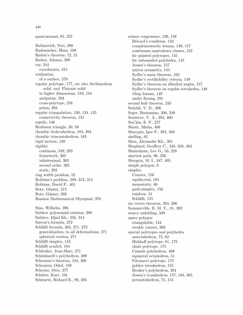
440

quasi-normal, 85, 227

Rabinovich, Yuri, 390Rademacher, Hans, 108Radon’s theorem, 12, 21Radon, Johann, 398ray, 244

coordinates, 315realization

of a surface, 279regular polytope, 177, see also Archimedean

solid and Platonic solidin higher dimensions, 183, 184antiprism, 394cross-polytope, 258prism, 394

regular triangulation, 130, 134, 135connectivity theorem, 131

reptile, 146Reuleaux triangle, 30, 50rhombic dodecahedron, 183, 394rhombic triacontahedron, 183rigid motion, 139rigidity

continous, 249, 293framework, 305infinitesimal, 302second order, 305static, 292

ring width problem, 52Robbins’s problem, 289, 313, 314Robbins, David P., 401Rote, Gunter, 215Rote, Gunter, 393Russian Mathematical Olympiad, 378

Suss, Wilhelm, 396Sabitov polynomial relation, 288Sabitov, Idjad Kh., 256, 314Sarron’s formula, 372Schlafli formula, 265, 271, 272

generalization, to all deformations, 271spherical version, 271

Schlafli simplex, 155Schlafli symbol, 184Schlenker, Jean-Marc, 271Schonhardt’s polyhedron, 388Schramm’s theorem, 104, 306Schramm, Oded, 108Schreier, Otto, 377Schutte, Kurt, 191Schwartz, Richard E., 90, 385

scissor congruence, 139, 158Bricard’s condition, 142complementarity lemma, 149, 157continuum equivalence classes, 153for painted polytopes, 145for unbounded polyhedra, 145Jessen’s theorem, 157mirror symmetry, 144Sydler’s main theorem, 162Sydler’s rectifiability criteria, 149Sydler’s theorem on dihedral angles, 157Sydler’s theorem on regular tetrahedra, 148tiling lemma, 149under flexing, 291

second hull theorem, 235Sedykh, V. D., 206Segre, Beniamino, 206, 240Senderov, V. A., 394, 400Sen’kin, E. P., 277Sharir, Micha, 406Sharygin, Igor F., 394, 403shelling, 82Shen, Alexander Kh., 381Shephard, Geoffrey C., 248, 358, 404Shnirelman, Lev G., 53, 228shortest path, 96, 356Shtogrin, M. I., 347, 405simple polygon, 8simplex

Coxeter, 156equifacetal, 184monostatic, 86path-simplex, 156rainbow, 21Schlafli, 155

six vertex theorem, 204, 206Sommerville, D. M. Y., 81, 392source unfolding, 349space polygon

triangulable, 134weakly convex, 200

special polytopes and polyhedraassociahedron, 75, 82Birkhoff polytope, 81, 175chain polytope, 175Csaszar polyhedron, 408equiareal octahedron, 51Fibonacci polytope, 175golden tetrahedron, 155Hooker’s polyhedron, 284Jessen’s icosahedron, 157, 183, 305permutohedron, 74, 154

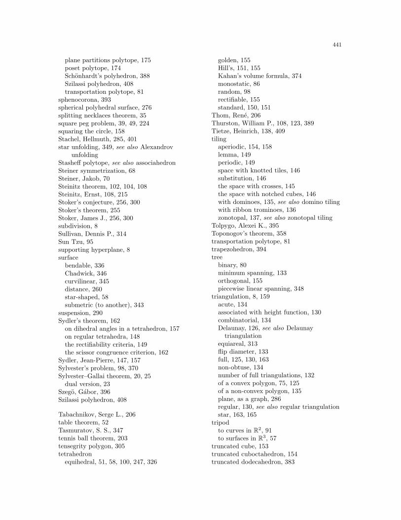
441

plane partitions polytope, 175poset polytope, 174Schonhardt’s polyhedron, 388Szilassi polyhedron, 408transportation polytope, 81

sphenocorona, 393spherical polyhedral surface, 276splitting necklaces theorem, 35square peg problem, 39, 49, 224squaring the circle, 158Stachel, Hellmuth, 285, 401star unfolding, 349, see also Alexandrov

unfoldingStasheff polytope, see also associahedronSteiner symmetrization, 68Steiner, Jakob, 70Steinitz theorem, 102, 104, 108Steinitz, Ernst, 108, 215Stoker’s conjecture, 256, 300Stoker’s theorem, 255Stoker, James J., 256, 300subdivision, 8Sullivan, Dennis P., 314Sun Tzu, 95supporting hyperplane, 8surface

bendable, 336Chadwick, 346curvilinear, 345distance, 260star-shaped, 58submetric (to another), 343

suspension, 290Sydler’s theorem, 162

on dihedral angles in a tetrahedron, 157on regular tetrahedra, 148the rectifiability criteria, 149the scissor congruence criterion, 162

Sydler, Jean-Pierre, 147, 157Sylvester’s problem, 98, 370Sylvester–Gallai theorem, 20, 25

dual version, 23Szego, Gabor, 396Szilassi polyhedron, 408

Tabachnikov, Serge L., 206table theorem, 52Tasmuratov, S. S., 347tennis ball theorem, 203tensegrity polygon, 305tetrahedron

equihedral, 51, 58, 100, 247, 326

golden, 155Hill’s, 151, 155Kahan’s volume formula, 374monostatic, 86random, 98rectifiable, 155standard, 150, 151

Thom, Rene, 206Thurston, William P., 108, 123, 389Tietze, Heinrich, 138, 409tiling

aperiodic, 154, 158lemma, 149periodic, 149space with knotted tiles, 146substitution, 146the space with crosses, 145the space with notched cubes, 146with dominoes, 135, see also domino tilingwith ribbon trominoes, 136zonotopal, 137, see also zonotopal tiling

Tolpygo, Alexei K., 395Toponogov’s theorem, 358transportation polytope, 81trapezohedron, 394tree

binary, 80minimum spanning, 133orthogonal, 155piecewise linear spanning, 348

triangulation, 8, 159acute, 134associated with height function, 130combinatorial, 134Delaunay, 126, see also Delaunay

triangulationequiareal, 313flip diameter, 133full, 125, 130, 163non-obtuse, 134number of full triangulations, 132of a convex polygon, 75, 125of a non-convex polygon, 135plane, as a graph, 286regular, 130, see also regular triangulationstar, 163, 165

tripodto curves in R2, 91to surfaces in R3, 57

truncated cube, 153truncated cuboctahedron, 154truncated dodecahedron, 383

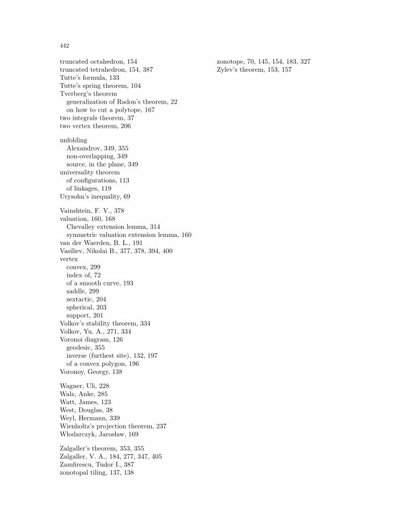
442

truncated octahedron, 154truncated tetrahedron, 154, 387Tutte’s formula, 133Tutte’s spring theorem, 104Tverberg’s theorem

generalization of Radon’s theorem, 22on how to cut a polytope, 167

two integrals theorem, 37two vertex theorem, 206

unfoldingAlexandrov, 349, 355non-overlapping, 349source, in the plane, 349

universality theoremof configurations, 113of linkages, 119

Urysohn’s inequality, 69

Vainshtein, F. V., 378valuation, 160, 168

Chevalley extension lemma, 314symmetric valuation extension lemma, 160

van der Waerden, B. L., 191Vasiliev, Nikolai B., 377, 378, 394, 400vertex

convex, 299index of, 72of a smooth curve, 193saddle, 299sextactic, 204spherical, 203support, 201

Volkov’s stability theorem, 334Volkov, Yu. A., 271, 334Voronoi diagram, 126

geodesic, 355inverse (furthest site), 132, 197of a convex polygon, 196

Voronoy, Georgy, 138

Wagner, Uli, 228Walz, Anke, 285Watt, James, 123West, Douglas, 38Weyl, Hermann, 339Wienholtz’s projection theorem, 237W lodarczyk, Jaros law, 169

Zalgaller’s theorem, 353, 355Zalgaller, V. A., 184, 277, 347, 405Zamfirescu, Tudor I., 387zonotopal tiling, 137, 138

zonotope, 70, 145, 154, 183, 327Zylev’s theorem, 153, 157