Lecture on Stellar/Binary Evolution & Population Synthesis

Ashley RuiterMax Planck Institute for Astrophysics

Garching, Germanyajr@mpa-garching.mpg.de

Mon. January 18 2010Pisa, Italy

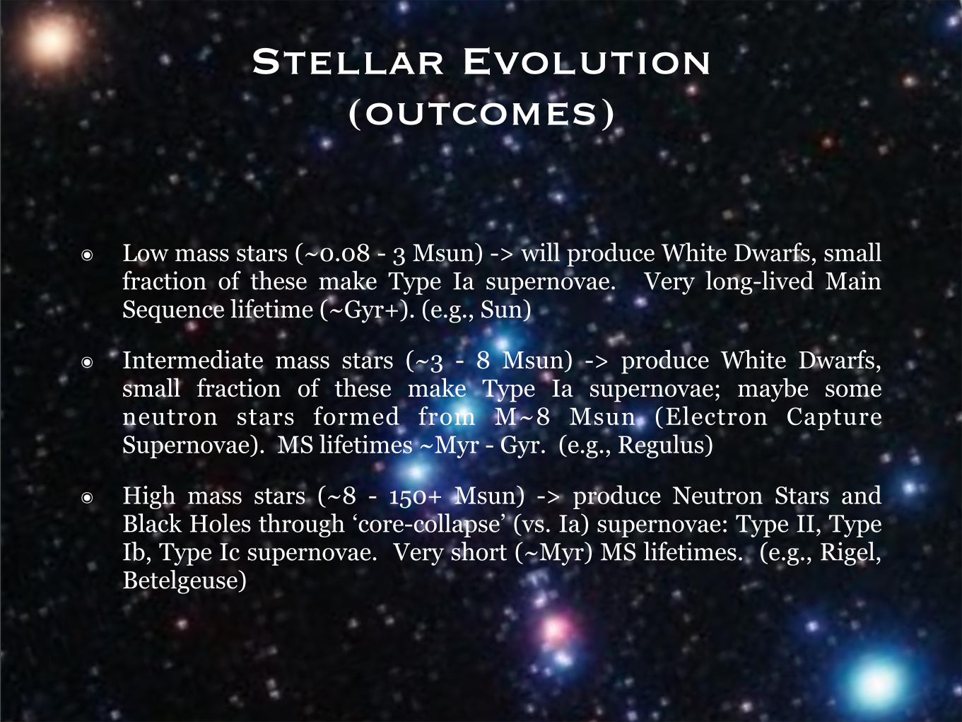
๏ Low mass stars (~0.08 - 3 Msun) -> will produce White Dwarfs, small fraction of these make Type Ia supernovae. Very long-lived Main Sequence lifetime (~Gyr+). (e.g., Sun)

๏ Intermediate mass stars (~3 - 8 Msun) -> produce White Dwarfs, small fraction of these make Type Ia supernovae; maybe some neutron stars formed from M~8 Msun (Electron Capture Supernovae). MS lifetimes ~Myr - Gyr. (e.g., Regulus)

๏ High mass stars (~8 - 150+ Msun) -> produce Neutron Stars and Black Holes through ‘core-collapse’ (vs. Ia) supernovae: Type II, Type Ib, Type Ic supernovae. Very short (~Myr) MS lifetimes. (e.g., Rigel, Betelgeuse)

Stellar Evolution(outcomes)

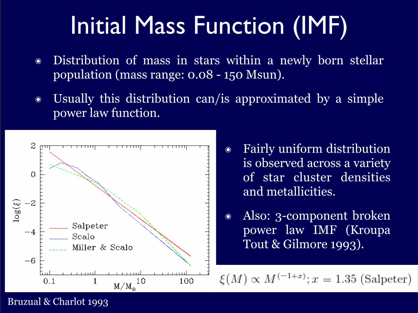
Initial Mass Function (IMF)๏ Distribution of mass in stars within a newly born stellar

population (mass range: 0.08 - 150 Msun).

๏ Usually this distribution can/is approximated by a simple power law function.

Bruzual & Charlot 1993

๏ Fairly uniform distribution is observed across a variety of star cluster densities and metallicities.

๏ Also: 3-component broken power law IMF (Kroupa Tout & Gilmore 1993).

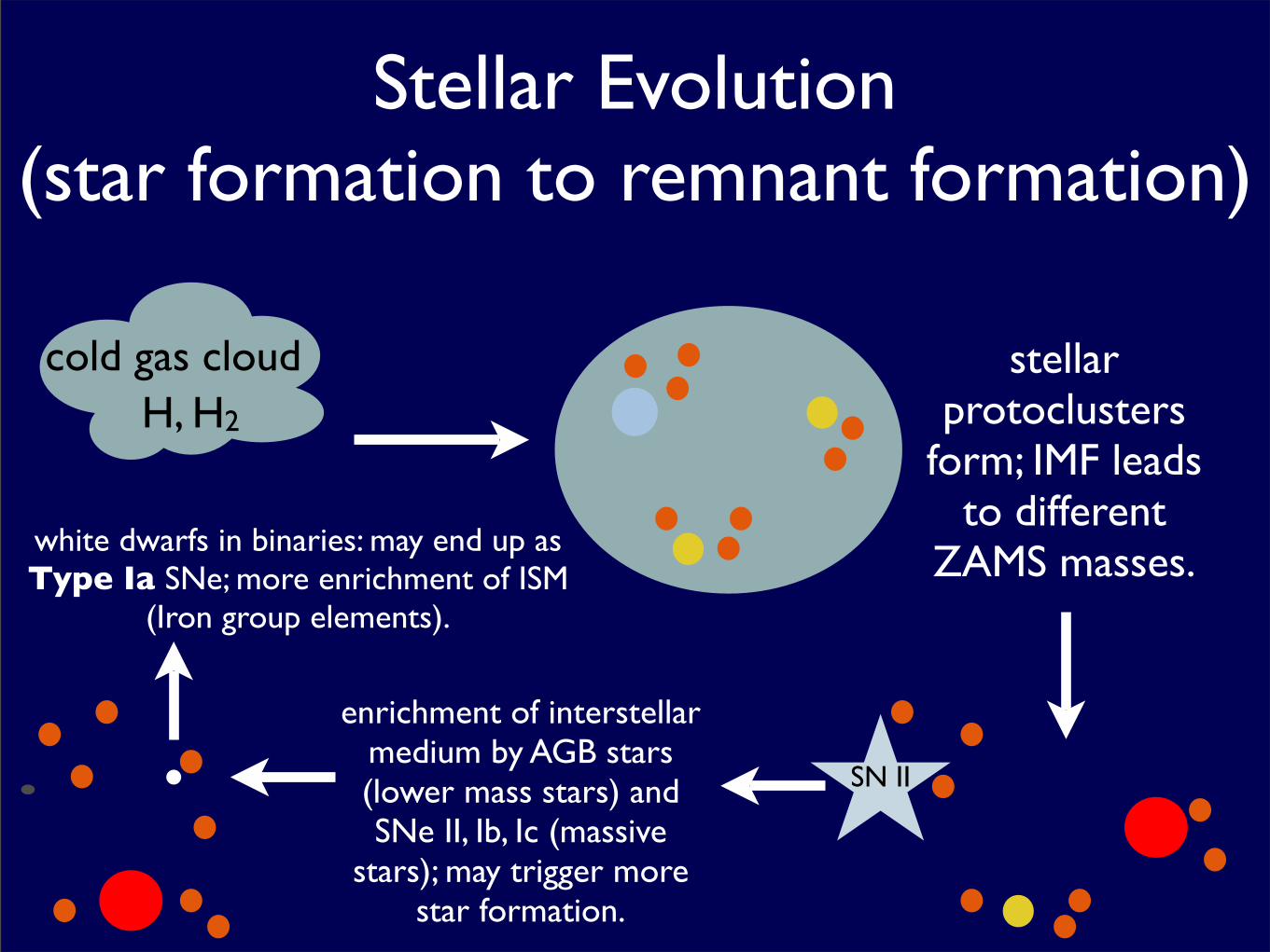
Stellar Evolution(star formation to remnant formation)

H, H2

cold gas cloud stellar protoclusters

form; IMF leads to different

ZAMS masses.

SN II

enrichment of interstellar medium by AGB stars (lower mass stars) and SNe II, Ib, Ic (massive

stars); may trigger more star formation.

white dwarfs in binaries: may end up as Type Ia SNe; more enrichment of ISM

(Iron group elements).

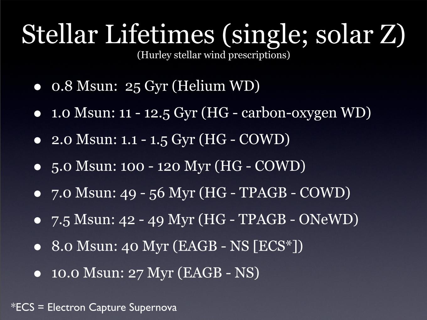
Stellar Lifetimes (single; solar Z)(Hurley stellar wind prescriptions)

• 0.8 Msun: 25 Gyr (Helium WD)

• 1.0 Msun: 11 - 12.5 Gyr (HG - carbon-oxygen WD)

• 2.0 Msun: 1.1 - 1.5 Gyr (HG - COWD)

• 5.0 Msun: 100 - 120 Myr (HG - COWD)

• 7.0 Msun: 49 - 56 Myr (HG - TPAGB - COWD)

• 7.5 Msun: 42 - 49 Myr (HG - TPAGB - ONeWD)

• 8.0 Msun: 40 Myr (EAGB - NS [ECS*])

• 10.0 Msun: 27 Myr (EAGB - NS)

*ECS = Electron Capture Supernova

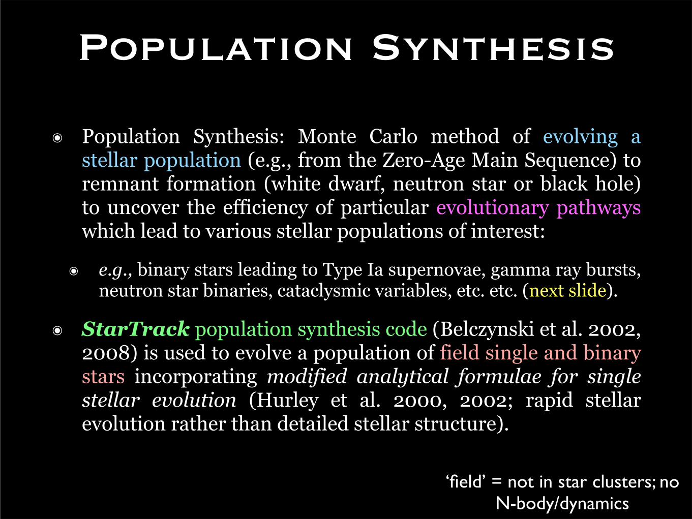
๏ Population Synthesis: Monte Carlo method of evolving a stellar population (e.g., from the Zero-Age Main Sequence) to remnant formation (white dwarf, neutron star or black hole) to uncover the efficiency of particular evolutionary pathways which lead to various stellar populations of interest:

๏ e.g., binary stars leading to Type Ia supernovae, gamma ray bursts, neutron star binaries, cataclysmic variables, etc. etc. (next slide).

๏ StarTrack population synthesis code (Belczynski et al. 2002, 2008) is used to evolve a population of field single and binary stars incorporating modified analytical formulae for single stellar evolution (Hurley et al. 2000, 2002; rapid stellar evolution rather than detailed stellar structure).

Population Synthesis

‘field’ = not in star clusters; no N-body/dynamics

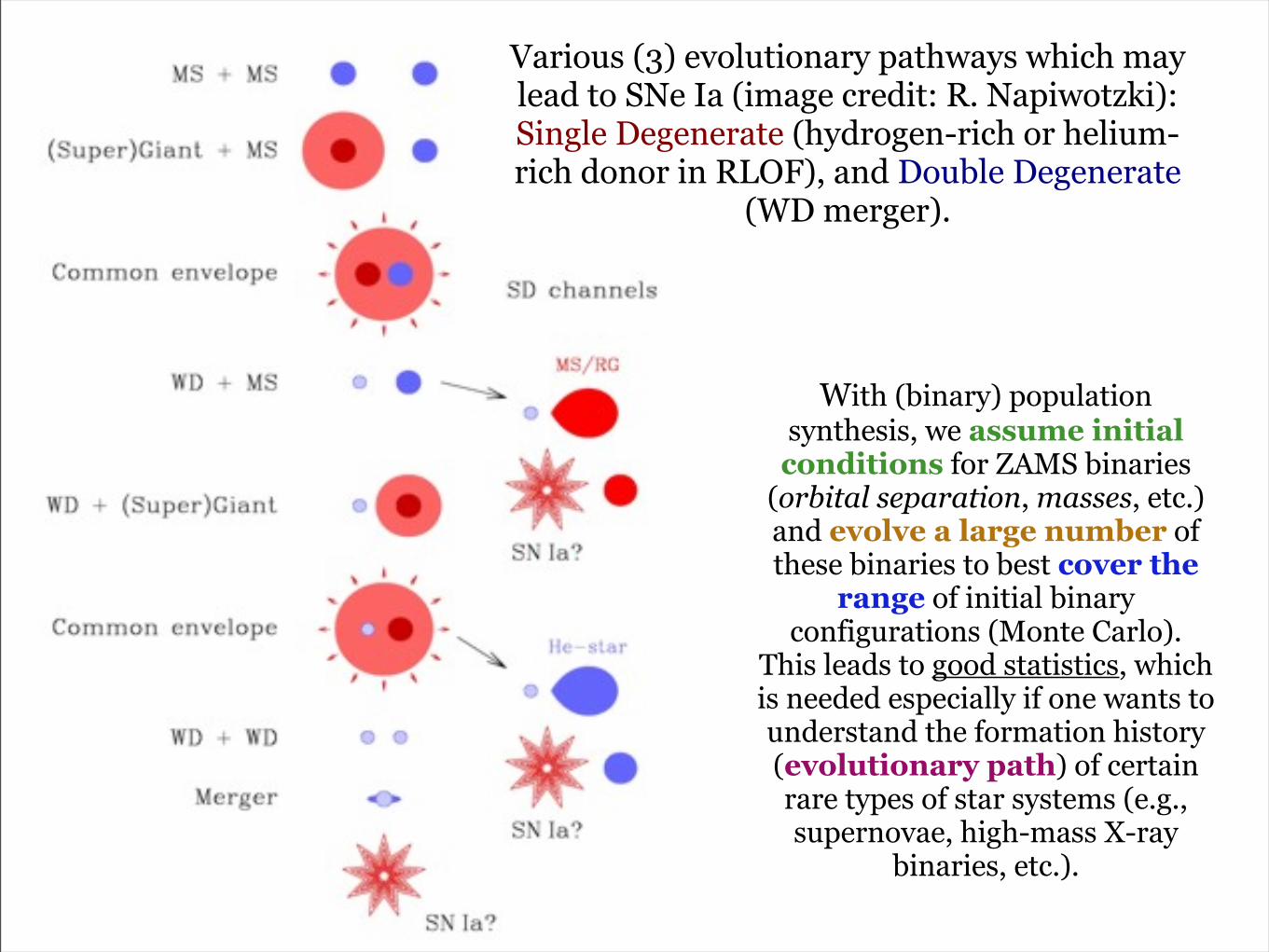
Various (3) evolutionary pathways which may lead to SNe Ia (image credit: R. Napiwotzki):Single Degenerate (hydrogen-rich or helium-rich donor in RLOF), and Double Degenerate

(WD merger).

With (binary) population synthesis, we assume initial conditions for ZAMS binaries

(orbital separation, masses, etc.) and evolve a large number of these binaries to best cover the

range of initial binary configurations (Monte Carlo).

This leads to good statistics, which is needed especially if one wants to understand the formation history (evolutionary path) of certain rare types of star systems (e.g., supernovae, high-mass X-ray

binaries, etc.).

Stellar Evolution

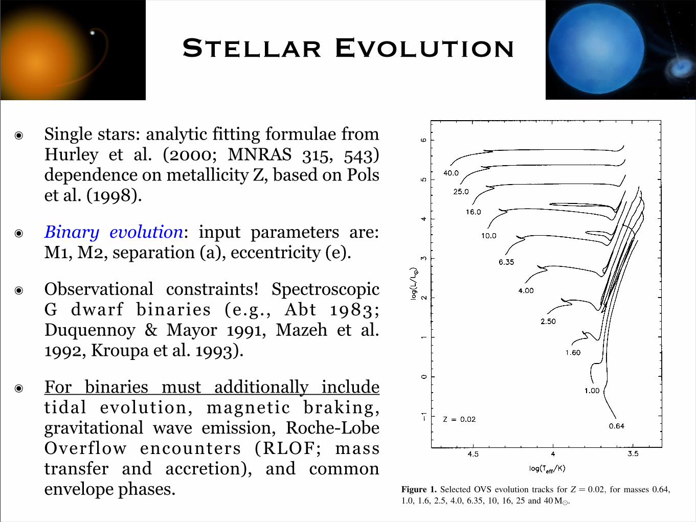
๏ Single stars: analytic fitting formulae from Hurley et al. (2000; MNRAS 315, 543) dependence on metallicity Z, based on Pols et al. (1998).

๏ Binary evolution: input parameters are: M1, M2, separation (a), eccentricity (e).

๏ Observational constraints! Spectroscopic G dwarf binaries (e.g., Abt 1983; Duquennoy & Mayor 1991, Mazeh et al. 1992, Kroupa et al. 1993).

๏ For binaries must additionally include tidal evolution, magnetic braking, gravitational wave emission, Roche-Lobe Overflow encounters (RLOF; mass transfer and accretion), and common envelope phases.

!"# $%&' &'( ')*+,-(. /'(00 1+,*23%.- 405,/& 400 ,6 &'( 025%.7

,/%&)8 9'( '(0%25 /'(00 604/' 34. +(1(4& %&/(06 54.) &%5(/: 4.* &'(

3)30( %/ ;.,$. 4/ 4 &'(+540 120/(8 9'%/ %/ &'( &'(+5400) 120/%.-

4/)51&,&%3 -%4.& <+4.3' =9>!"#?8

9'( /&(004+ +4*%2/ 34. -+,$ &, @(+) 04+-( @402(/ ,. &'( !"#A

&'%/ 0,$(+/ &'( /2+643( -+4@%&) ,6 &'( /&4+: /, &'4& &'( /2+643(

54&(+%40 %/ 0(// &%-'&0) <,2.*8 9'2/ 54//70,// 6+,5 &'( /&(004+

/2+643( 34. <(3,5( /%-.%6%34.&: $%&' &'( +4&( ,6 54//70,// 43&2400)

433(0(+4&%.- $%&' &%5( *2+%.- 3,.&%.2(* (@,02&%,. 21 &'( !"#8

B.6,+&2.4&(0): ,2+ 2.*(+/&4.*%.- ,6 &'( 5(3'4.%/5/ &'4& 342/(

&'%/ 54//70,// %/ 1,,+: $%&' 1,//%<0( /2--(/&%,./ 0%.;%.- %& &, &'(

'(0%25 /'(00 604/'(/ ,+ &, 1(+%,*%3 (.@(0,1( 120/4&%,./8 C'4&(@(+

&'( 342/(: &'( %.602(.3( ,. &'( (@,02&%,. ,6 !"# /&4+/ %/

/%-.%6%34.&8 D4//70,// $%00 (@(.&2400) +(5,@( 400 ,6 &'( /&4+/

(.@(0,1( /, &'4& &'( ')*+,-(.7<2+.%.- /'(00 /'%.(/ &'+,2-'8 9'(

/&4+ &'(. 0(4@(/ &'( !"# 4.* (@,0@(/ &, '%-'(+ !(66 4& .(4+0)

3,./&4.& 025%.,/%&)8 !/ &'( 1',&,/1'(+( -(&/ ',&&(+: &'( (.(+-(&%3

1',&,./ <(3,5( 4</,+<(* <) &'( 54&(+%40 $'%3' $4/ &'+,$. ,66

$'%0( ,. &'( !"#8 9'%/ 342/(/ &'( 54&(+%40 &, +4*%4&(: 4.* &'( /&4+

54) <( /((. 4/ 4 104.(&4+) .(<2048 9'( 3,+( ,6 &'( /&4+ &'(. <(-%./

&, 64*( 4/ &'( .230(4+ <2+.%.- 3(4/(/8 9'( /&4+ %/ .,$ 4 $'%&(

*$4+6 =CE? 4.* 3,,0/ /0,$0) 4& '%-' &(51(+4&2+( <2& 0,$

025%.,/%&)8

F6 &'( 54// ,6 &'( /&4+ %/ 04+-( (.,2-': " ! GD!! &'( 34+<,.7,H)-(. 3,+( %/ .,& *(-(.(+4&( 4.* $%00 %-.%&( 34+<,. 4/ %&

3,.&+43&/: 6,00,$(* <) 4 /233(//%,. ,6 .230(4+ +(43&%,. /(I2(.3(/

$'%3' @(+) I2%3;0) 1+,*23( 4. %..(+ %+,. 3,+(8 !.) 62+&'(+

+(43&%,./ 4+( (.*,&'(+5%3 4.* 34..,& 3,.&+%<2&( &, &'( 025%.,/%&)

,6 &'( /&4+8 >',&,*%/%.&(-+4&%,. ,6 %+,.: 3,5<%.(* $%&' (0(3&+,.

341&2+( <) 1+,&,./ 4.* '(4@) .230(%: &'(. +(5,@(/ 5,/& ,6 &'(

(0(3&+,. *(-(.(+43) 1+(//2+( &'4& $4/ /211,+&%.- &'( 3,+(: 4.* %&

<(-%./ &, 3,0041/( +41%*0)8 C'(. &'( *(./%&) <(3,5(/ 04+-(

(.,2-': &'( %..(+ 3,+( +(<,2.*/: /(.*%.- 4 /',3;$4@( ,2&$4+*/

&'+,2-' &'( ,2&(+ 04)(+/ ,6 &'( /&4+ &'4& '4@( +(54%.(* /2/1(.*(*

4<,@( &'( 3,0041/%.- 3,+(8 !/ 4 +(/20&: &'( (.@(0,1( ,6 &'( /&4+ %/

(J(3&(* %. 4 /21(+.,@4 =KL? (H10,/%,.: /, &'4& &'( !"# %/

(66(3&%@(0) &+2.34&(* 4& &'( /&4+& ,6 34+<,. <2+.%.- 4.* &'( /&4+ '4/

., 9>!"# 1'4/(8 9'( +(5.4.& %. &'( %..(+ 3,+( $%00 /&4<%0%M( &,

6,+5 4 .(2&+,. /&4+ =LK? /211,+&(* <) .(2&+,. *(-(.(+43)

1+(//2+(: 2.0(// &'( %.%&%40 /&(004+ 54// %/ 04+-( (.,2-' &'4&

3,510(&( 3,0041/( &, 4 <043; ',0( =#N? ,332+/8

K&4+/ $%&' " ! OPD! 4+( /(@(+(0) 466(3&(* <) 54//70,//

*2+%.- &'(%+ (.&%+( (@,02&%,. 4.* 54) 0,/( &'(%+ (.@(0,1(/ *2+%.-

QN(#: ,+ (@(. ,. &'( N": (H1,/%.- .230(4+ 1+,3(//(* 54&(+%408 F6

&'%/ ,332+/: &'(. 4 .4;(* '(0%25 /&4+ %/ 1+,*23(* 4.* /23' /&4+/: ,+

/&4+/ 4<,2& &, <(3,5( .4;(* '(0%25 /&4+/: 54) <( C,06RS4)(&

/&4+/8 C,06RS4)(& /&4+/ 4+( 54//%@( ,<J(3&/ $'%3' 4+( 6,2.* .(4+

&'( DK: 4+( 0,/%.- 54// 4& @(+) '%-' +4&(/: 4.* /',$ $(4;: ,+ .,:

')*+,-(. 0%.(/ %. &'(%+ /1(3&+48 T25%.,2/ <02( @4+%4<0(/ =T#U/?

4+( (H&+(5(0) 54//%@( 1,/&7DK ,<J(3&/ $%&' (.,+5,2/ 54//70,//

+4&(/ %. 4 /&4-( ,6 (@,02&%,. J2/& 1+%,+ &, <(3,5%.- C,06RS4)(&

/&4+/8 L4;(* '(0%25 /&4+/ 34. 40/, <( 1+,*23(* 6+,5 0(// 54//%@(

/&4+/ %. <%.4+%(/ 4/ 4 3,./(I2(.3( ,6 54// &+4./6(+8

U4+%4&%,./ %. 3,51,/%&%,. 34. 40/, 466(3& &'( /&(004+ (@,02&%,.

&%5(7/340(/ 4/ $(00 4/ &'( 411(4+4.3( ,6 &'( (@,02&%,. ,. &'( NSE:

4.* (@(. &'( 20&%54&( 64&( ,6 &'( /&4+8 ! 5,+( *(&4%0(* *%/32//%,.

,6 &'( @4+%,2/ 1'4/(/ ,6 (@,02&%,. 34. <( 6,2.* &'+,2-',2& &'%/

141(+8

!"#$%& '( K(0(3&(* VUK (@,02&%,. &+43;/ 6,+ # ! W"WX! 6,+ 54//(/ W8YZ:O8W: O8Y: X8P: Z8W: Y8[P: OW: OY: XP 4.* ZWD!8

!"#$%& )( K45( 4/ \%-8 O 6,+ # ! W"WWO" 9'( O8W7D! 1,/&7'(0%25 604/'

&+43; '4/ <((. ,5%&&(* 6,+ 304+%&)8

$%&'()*)+,-.) /+/012-3 4%(&50/) 4%( ,2)00/( ).%052-%+ PZP

! XWWW S!K: DLS!K *'+: PZ[RPY]

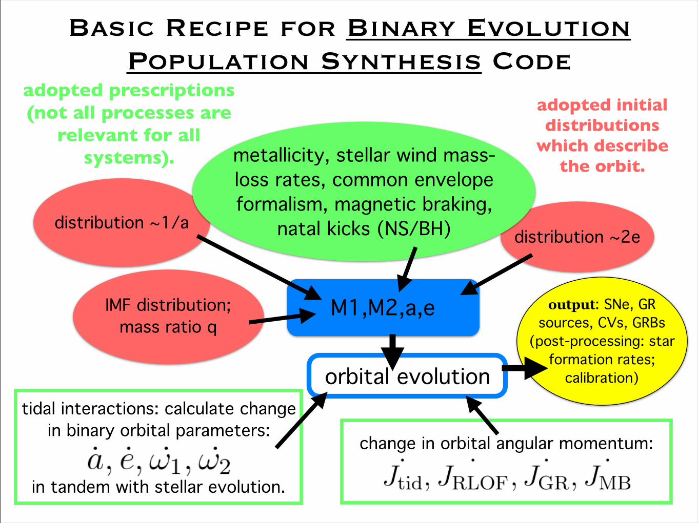
Basic Recipe for Binary Evolution Population Synthesis Code

M1,M2,a,eIMF distribution;mass ratio q

distribution ~1/a

metallicity, stellar wind mass-loss rates, common envelope formalism, magnetic braking,

natal kicks (NS/BH)

adopted prescriptions (not all processes are

relevant for all systems).

adopted initial distributions

which describe the orbit.

distribution ~2e

orbital evolutiontidal interactions: calculate change

in binary orbital parameters:

in tandem with stellar evolution.

change in orbital angular momentum:

output: SNe, GR sources, CVs, GRBs

(post-processing: star formation rates;

calibration)

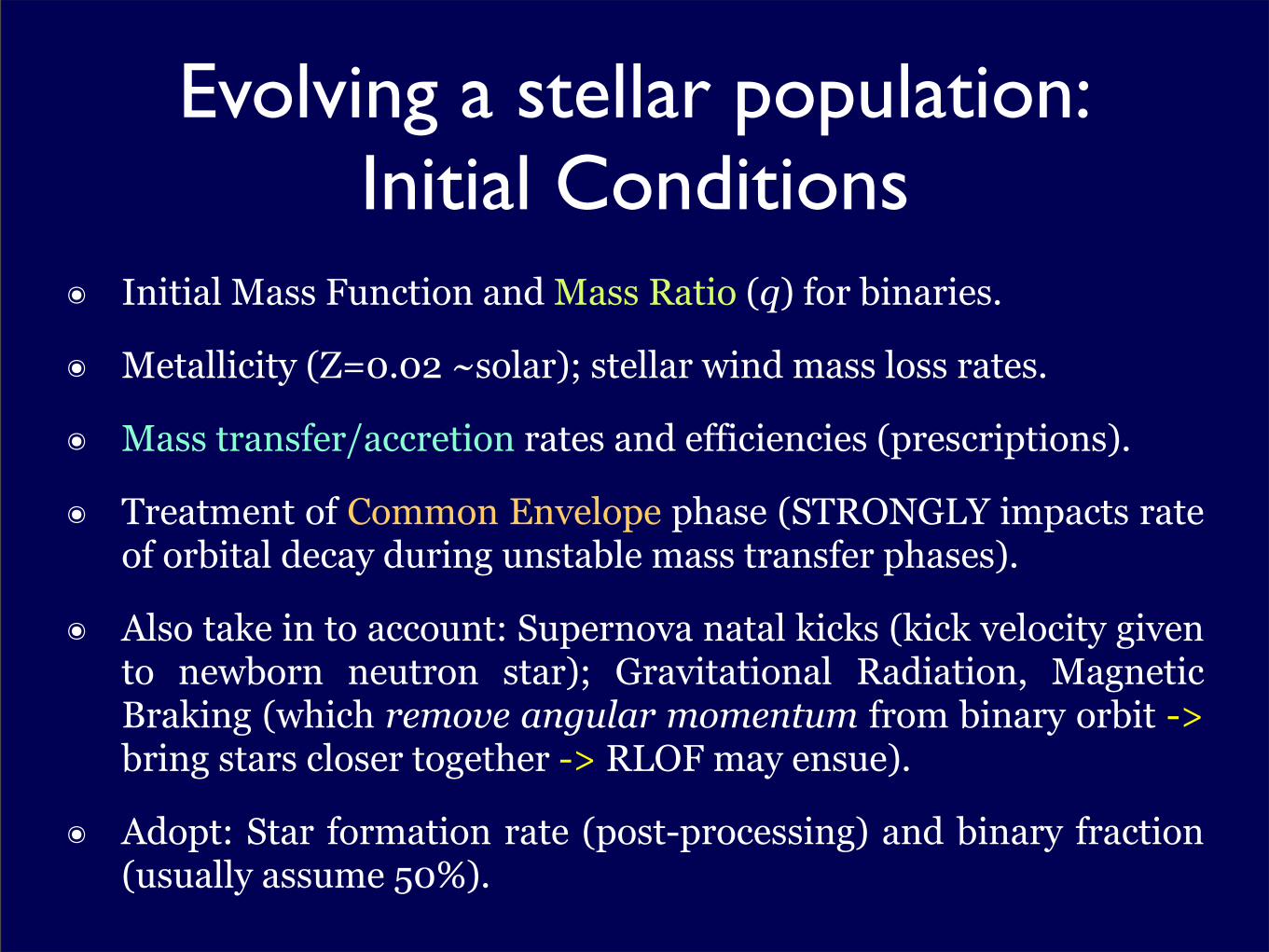
Evolving a stellar population:Initial Conditions

๏ Initial Mass Function and Mass Ratio (q) for binaries.

๏ Metallicity (Z=0.02 ~solar); stellar wind mass loss rates.

๏ Mass transfer/accretion rates and efficiencies (prescriptions).

๏ Treatment of Common Envelope phase (STRONGLY impacts rate of orbital decay during unstable mass transfer phases).

๏ Also take in to account: Supernova natal kicks (kick velocity given to newborn neutron star); Gravitational Radiation, Magnetic Braking (which remove angular momentum from binary orbit -> bring stars closer together -> RLOF may ensue).

๏ Adopt: Star formation rate (post-processing) and binary fraction (usually assume 50%).

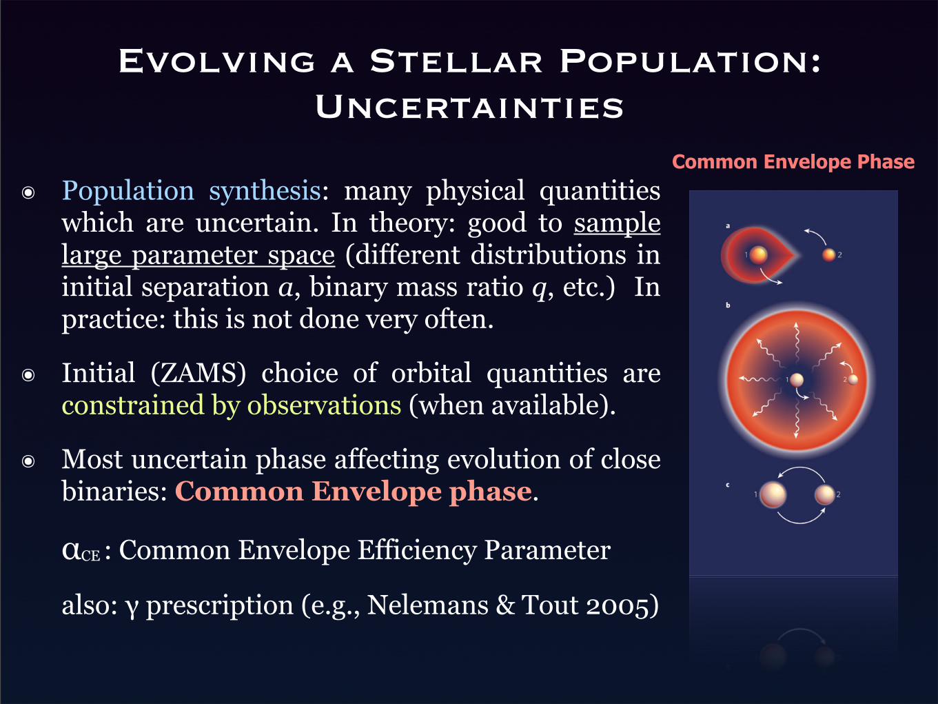
Evolving a Stellar Population: Uncertainties

๏ Population synthesis: many physical quantities which are uncertain. In theory: good to sample large parameter space (different distributions in initial separation a, binary mass ratio q, etc.) In practice: this is not done very often.

๏ Initial (ZAMS) choice of orbital quantities are constrained by observations (when available).

๏ Most uncertain phase affecting evolution of close binaries: Common Envelope phase.

αCE : Common Envelope Efficiency Parameter

also: γ prescription (e.g., Nelemans & Tout 2005)

Common Envelope Phase

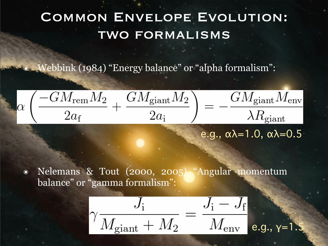
๏ Nelemans & Tout (2000, 2005) “Angular momentum balance” or “gamma formalism”:

๏ Webbink (1984) “Energy balance” or “alpha formalism”:

Common Envelope Evolution:two formalisms

e.g., αλ=1.0, αλ=0.5

e.g., γ=1.5

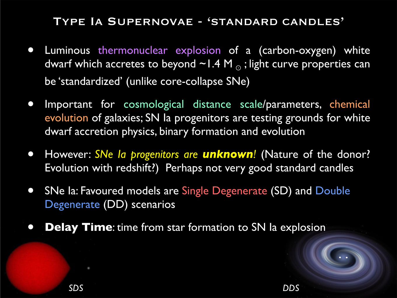
• Luminous thermonuclear explosion of a (carbon-oxygen) white dwarf which accretes to beyond ~1.4 M☉; light curve properties can

be ‘standardized’ (unlike core-collapse SNe)

• Important for cosmological distance scale/parameters, chemical evolution of galaxies; SN Ia progenitors are testing grounds for white dwarf accretion physics, binary formation and evolution

• However: SNe Ia progenitors are unknown! (Nature of the donor? Evolution with redshift?) Perhaps not very good standard candles

• SNe Ia: Favoured models are Single Degenerate (SD) and Double Degenerate (DD) scenarios

• Delay Time: time from star formation to SN Ia explosion

Type Ia Supernovae - ‘standard candles’

SDS DDS

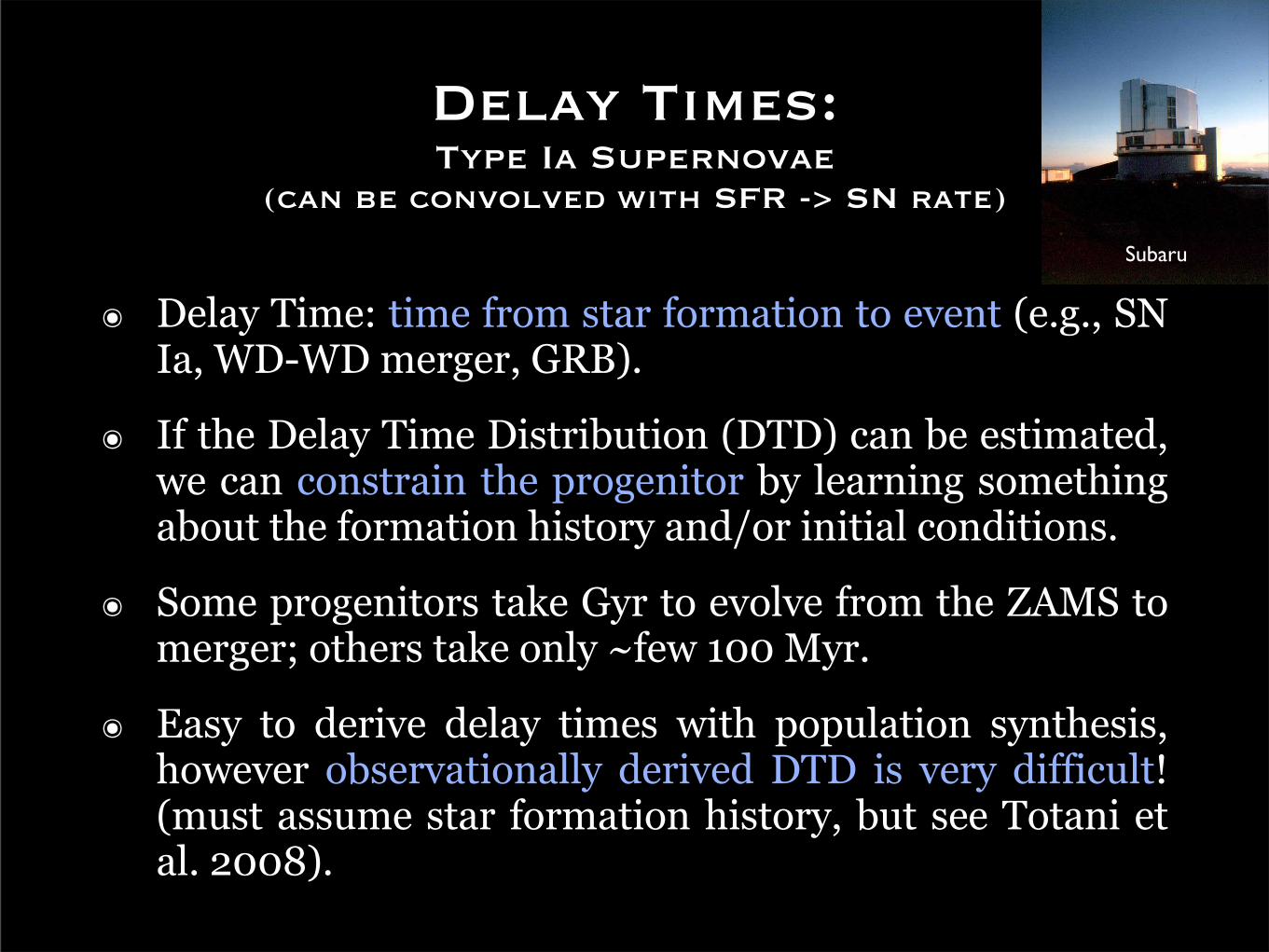
Delay Times:Type Ia Supernovae

(can be convolved with SFR -> SN rate)

Subaru

๏ Delay Time: time from star formation to event (e.g., SN Ia, WD-WD merger, GRB).

๏ If the Delay Time Distribution (DTD) can be estimated, we can constrain the progenitor by learning something about the formation history and/or initial conditions.

๏ Some progenitors take Gyr to evolve from the ZAMS to merger; others take only ~few 100 Myr.

๏ Easy to derive delay times with population synthesis, however observationally derived DTD is very difficult! (must assume star formation history, but see Totani et al. 2008).

1338 T. Totani et al. [Vol. 60,

Table 4. Examination of systematic errors in the DTD measurements.!

Analysis fD(tIa) [century"1.1010LK;0;ˇ/"1] in tIa bins [Gyr] fD;1Gyr ˛

0.1–0.25 0.25–0.5 0.5–1.0 1.0–2.0 2.0–4.0 4.0–8.0

Baseline 2.89+1:60"1:20 1.98+0:96

"0:73 0.84+0:30"0:24 0.49+0:17

"0:13 0.12+0:38"0:12 0.00+1:08

"0:00 0.55+0:12"0:11 "1.08+0:15

"0:15

tIa = ht!i 3.12+1:64"1:21 2.87+1:26

"0:96 0.89+0:36"0:28 0.52+0:16

"0:13 0.56+0:42"0:27 0.00+0:47

"0:00 0.63+0:14"0:12 "1.09+0:15

"0:15

tga=!SF # 3.0 7.18+5:65"3:61 2.81+1:76

"1:23 0.84+0:33"0:26 0.45+0:17

"0:13 0.17+0:47"0:17 0.00+1:19

"0:00 0.65+0:17"0:14 "1.23+0:18

"0:17

Prompt $ 2.5 2.32+1:60"1:20 1.70+0:96

"0:73 0.77+0:30"0:24 0.46+0:17

"0:13 0.11+0:38"0:11 0.00+1:07

"0:00 0.50+0:12"0:12 "1.05+0:16

"0:15

Solar Z 1.64+0:81"0:62 1.65+0:84

"0:63 0.74+0:40"0:30 0.48+0:16

"0:13 0.30+0:19"0:13 0.14+0:38

"0:14 0.47+0:11"0:10 "0.92+0:15

"0:13

Chabrier IMF 3.00+1:65"1:23 2.56+1:15

"0:89 0.93+0:34"0:27 0.40+0:17

"0:13 0.30+0:48"0:23 0.00+0:84

"0:00 0.57+0:13"0:12 "1.11+0:15

"0:15

KA97 6.43+2:65"2:08 4.87+1:43

"1:18 0.87+0:55"0:39 0.36+0:25

"0:17 0.38+0:33"0:20 0.43+1:02

"0:37 0.79+0:19"0:16 "1.27+0:14

"0:14

AV < 0.5 3.27+2:88"1:97 2.48+1:57

"1:15 1.00+0:47"0:36 0.59+0:20

"0:16 0.00+0:35"0:00 0.00+1:35

"0:00 0.64+0:17"0:16 "1.16+0:17

"0:16

SN +0.3 mag 3.21+1:78"1:34 2.21+1:07

"0:82 0.94+0:34"0:27 0.54+0:18

"0:15 0.14+0:42"0:14 0.00+1:22

"0:00 0.60+0:13"0:12 "1.11+0:15

"0:15

SN "0.3 mag 2.58+1:44"1:07 1.75+0:85

"0:65 0.75+0:27"0:21 0.43+0:15

"0:12 0.11+0:33"0:11 0.00+0:96

"0:00 0.50+0:11"0:10 "1.05+0:15

"0:15

! Various DTD results are shown when the analysis method was changed from the baseline analysis. The last two columns show the best-fitpower-law DTD, fD(tIa) = fD;1Gyr (tIa=1Gyr)˛ . The “tIa = ht!i” results were obtained by estimating tIa simply by the mean stellarage, ht!i, of the host galaxies (open squares in figure 7). The “tga=!SF # 3.0” results were obtained when a more strict criterion ofthe old galaxies was applied than in the baseline analysis. The “prompt$ 2.5” results were obtained when the fraction of the prompt Iapopulation was increased by a factor of 2.5 from the baseline analysis. The “solar Z”, “Chabrier IMF”, and “KA97” results were obtainedusing stellar age and mass estimates with a different metallicity, a different IMF, and a different stellar population synthesis model fromthe baseline analysis, respectively. The “AV < 0.5” results were obtained with a more strict cut about the dust extinction of host galaxies.The “SN ˙ 0.3 mag” results were obtained with the SN Ia light curve ˙ 0.3 mag fainter/brighter than in the baseline analysis. All errorsare in statistical 1 " .

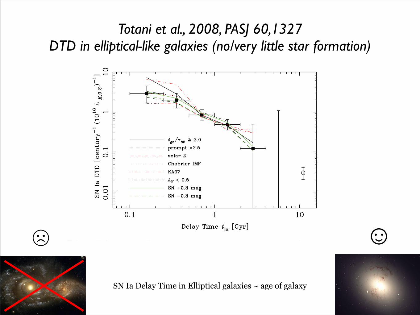
Fig. 9. SN Ia DTD fD(tIa) estimated by different prescriptions from the baseline analysis, shown by lines. The data points are for the baseline analysis,which are the same as those in figure 7. The labels for the lines are the same as in table 4. See this table and the main text for explanations.

of M!=M!;bl. This is most likely a result of the limited SFhistory template in estimates using the KA97 model (only 1template corresponding to !SF % 0.1 Gyr). It is expected that

the age estimates with a single small value of !SF tend to under-estimate the true age, and this trend is in fact seen in the leftpanel of figure 10. The underestimate in stellar age would

Totani et al., 2008, PASJ 60,1327DTD in elliptical-like galaxies (no/very little star formation)

SN Ia Delay Time in Elliptical galaxies ~ age of galaxy

☺☹

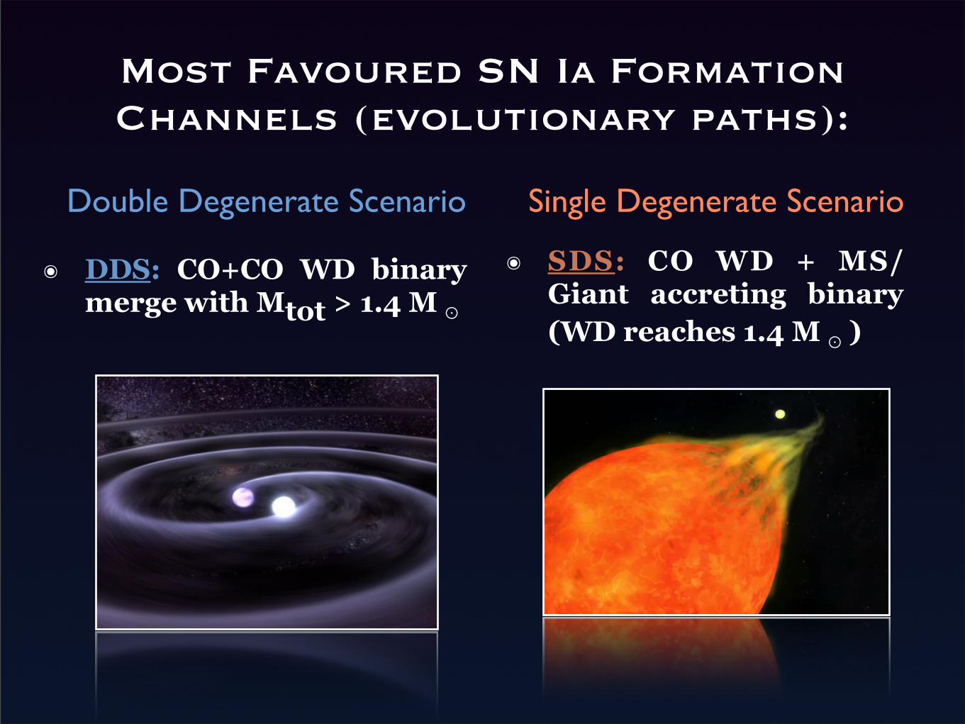
Most Favoured SN Ia Formation Channels (evolutionary paths):

๏ DDS: CO+CO WD binary merge with Mtot > 1.4 M☉

๏ SDS: CO WD + MS/Giant accreting binary (WD reaches 1.4 M☉)

Double Degenerate Scenario Single Degenerate Scenario

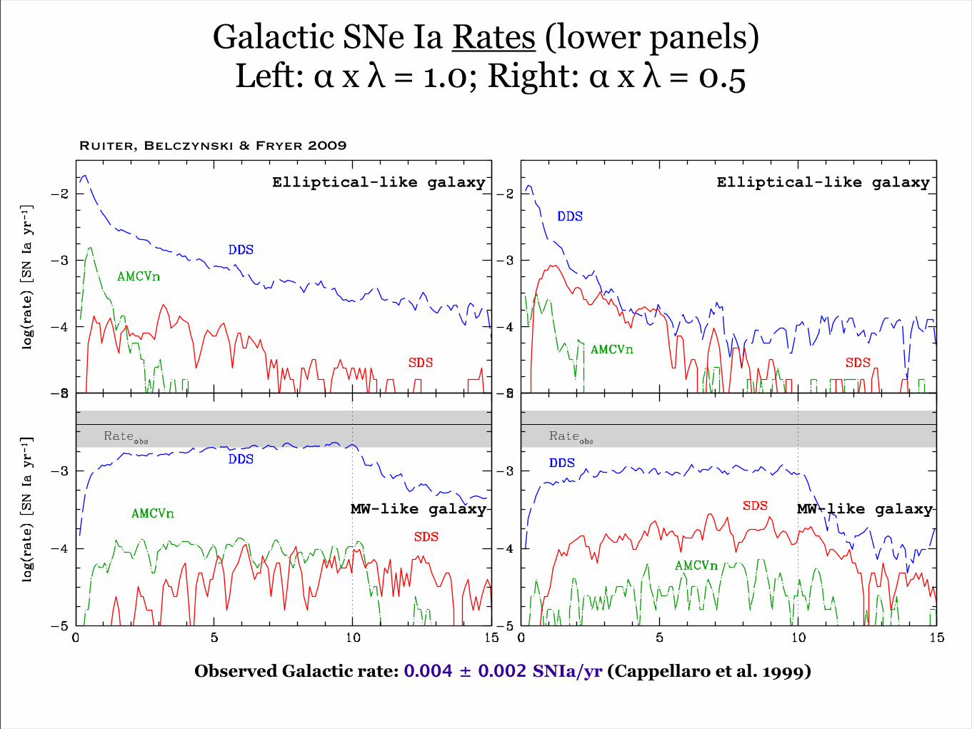
Galactic SNe Ia Rates (lower panels) Left: α x λ = 1.0; Right: α x λ = 0.5

Ruiter, Belczynski & Fryer 2009

Observed Galactic rate: 0.004 ± 0.002 SNIa/yr (Cappellaro et al. 1999)

Elliptical-like galaxy Elliptical-like galaxy

MW-like galaxyMW-like galaxy

some credits!

• http://physics.uoregon.edu/~jimbrau/BrauImNew/Chap20/FG20_08.jpg

• http://star.herts.ac.uk/progs/images/whitedwarf3.jpg

• http://astronomy.swin.edu.au/cms/imagedb/albums/userpics/hrdiagram1.jpg