lecture notes on c-algebras - uvic-algebras.pdf · lecture notes on c-algebras ian f. putnam july...
TRANSCRIPT
Lecture Notes on C∗-algebras
Ian F. Putnam
July 28, 2016

2
Contents
1 Basics of C∗-algebras 51.1 Definition . . . . . . . . . . . . . . . . . . . . . . . . . . . . . 51.2 Examples . . . . . . . . . . . . . . . . . . . . . . . . . . . . . 71.3 Spectrum . . . . . . . . . . . . . . . . . . . . . . . . . . . . . 91.4 Commutative C∗-algebras . . . . . . . . . . . . . . . . . . . . 131.5 Further consequences of the C∗-condition . . . . . . . . . . . . 191.6 Positivity . . . . . . . . . . . . . . . . . . . . . . . . . . . . . 211.7 Finite-dimensional C∗-algebras . . . . . . . . . . . . . . . . . . 241.8 Non-unital C∗-algebras . . . . . . . . . . . . . . . . . . . . . . 321.9 Ideals and quotients . . . . . . . . . . . . . . . . . . . . . . . 361.10 Traces . . . . . . . . . . . . . . . . . . . . . . . . . . . . . . . 401.11 Representations . . . . . . . . . . . . . . . . . . . . . . . . . . 421.12 The GNS construction . . . . . . . . . . . . . . . . . . . . . . 481.13 von Neumann algebras . . . . . . . . . . . . . . . . . . . . . . 57
2 Group C∗-algebras 632.1 Group representations . . . . . . . . . . . . . . . . . . . . . . 632.2 Group algebras . . . . . . . . . . . . . . . . . . . . . . . . . . 652.3 Finite groups . . . . . . . . . . . . . . . . . . . . . . . . . . . 672.4 The C∗-algebra of a discrete group . . . . . . . . . . . . . . . 692.5 Abelian groups . . . . . . . . . . . . . . . . . . . . . . . . . . 752.6 The infinite dihedral group . . . . . . . . . . . . . . . . . . . . 772.7 The group F2 . . . . . . . . . . . . . . . . . . . . . . . . . . . 832.8 Locally compact groups . . . . . . . . . . . . . . . . . . . . . 89
3 Groupoid C∗-algebras 953.1 Groupoids . . . . . . . . . . . . . . . . . . . . . . . . . . . . . 963.2 Topological groupoids . . . . . . . . . . . . . . . . . . . . . . . 101
3
4 CONTENTS
3.3 The C∗-algebra of an etale groupoid . . . . . . . . . . . . . . . 1053.3.1 The fundamental lemma . . . . . . . . . . . . . . . . . 1053.3.2 The ∗-algebra Cc(G) . . . . . . . . . . . . . . . . . . . 1063.3.3 The left regular representation . . . . . . . . . . . . . . 1113.3.4 C∗(G) and C∗r (G) . . . . . . . . . . . . . . . . . . . . . 114
3.4 The structure of groupoid C∗-algebras . . . . . . . . . . . . . 1173.4.1 The expectation onto C(G0) . . . . . . . . . . . . . . . 1173.4.2 Traces on groupoid C∗-algebras . . . . . . . . . . . . . 1193.4.3 Ideals in groupoid C∗-algebras . . . . . . . . . . . . . . 124
3.5 AF-algebras . . . . . . . . . . . . . . . . . . . . . . . . . . . . 134
Chapter 1
Basics of C∗-algebras
1.1 Definition
We begin with the definition of a C∗-algebra.
Definition 1.1.1. A C∗-algebra A is a (non-empty) set with the followingalgebraic operations:
1. addition, which is commutative and associative
2. multiplication, which is associative
3. multiplication by complex scalars
4. an involution a 7→ a∗ (that is, (a∗)∗ = a, for all a in A)
Both types of multiplication distribute over addition. For a, b in A, we have(ab)∗ = b∗a∗. The involution is conjugate linear; that is, for a, b in A and λin C, we have (λa + b)∗ = λa∗ + b∗. For a, b in A and λ, µ in C, we haveλ(ab) = (λa)b = a(λb) and (λµ)a = λ(µa).
In addition, A has a norm in which it is a Banach algebra; that is,
‖λa‖ = |λ|‖a‖,‖a+ b‖ ≤ ‖a‖+ ‖b‖,‖ab‖ ≤ ‖a‖‖b‖,
for all a, b in A and λ in C, and A is complete in the metric d(a, b) = ‖a−b‖.Finally, for all a in A, we have ‖a∗a‖ = ‖a‖2.
5
6 CHAPTER 1. BASICS OF C∗-ALGEBRAS
Very simply, A has an algebraic structure and a topological structurecoming from a norm. The condition that A be a Banach algebra expressesa compatibility between these structures. The final condition, usually re-ferred to as the C∗-condition, may seem slightly mysterious, but it is a verystrong link between the algebraic and topological structures, as we shall seepresently.
It is probably also worth mentioning two items which are not axioms.First, the algebra need not have a unit for the multiplication. If it doeshave a unit, we write it as 1 or 1A and say that A is unital. Secondly, themultiplication is not necessarily commutative. That is, it is not generally thecase that ab = ba, for all a, b. The first of these two issues turns out to be arelatively minor one (which will be dealt with in Section 1.8). The latter isessential and, in many ways, is the heart of the subject.
One might have expected an axiom stating that the involution is isomet-ric. In fact, it is a simple consequence of the ones given, particularly theC∗-condition.
Proposition 1.1.2. If a is an element of a C∗-algebra A, then ‖a‖ = ‖a∗‖.
Proof. As A is a Banach algebra ‖a‖2 = ‖a∗a‖ ≤ ‖a∗‖‖a‖ and so ‖a‖ ≤ ‖a∗‖.Replacing a with a∗ then yields the result.
Next, we introduce some terminology for elements in a C∗-algebra. For agiven a in A, the element a∗ is usually called the adjoint of a. The first termin the following definition is then rather obvious. The second is much lessso, but is used for historical reasons from operator theory. The remainingterms all have a geometric flavour. If one considers the elements in B(H),operators on a Hilbert space, each of these purely algebraic terms can be givenan equivalent formulation in geometric terms of the action of the operatoron the Hilbert space.
Definition 1.1.3. Let A be a C∗-algebra.
1. An element a is self-adjoint if a∗ = a.
2. An element a is normal if a∗a = aa∗.
3. An element p is a projection if p2 = p = p∗; that is, p is a self-adjointidempotent.
1.2. EXAMPLES 7
4. Assuming that A is unital, an element u is a unitary if u∗u = 1 = uu∗;that is, u is invertible and u−1 = u∗.
5. Assuming that A is unital, an element u is an isometry if u∗u = 1.
6. An element u is a partial isometry if u∗u is a projection.
7. An element a is positive if it may be written a = b∗b, for some b in A.In this case, we often write a ≥ 0 for brevity.
1.2 Examples
Example 1.2.1. C, the complex numbers. More than just an example, it isthe prototype.
Example 1.2.2. Let H be a complex Hilbert space with inner product denoted< ·, · >. The collection of bounded linear operators on H, denoted by B(H),is a C∗-algebra. The linear structure is clear. The product is by compositionof operators. The ∗ operation is the adjoint; for any operator a on H, itsadjoint is defined by the equation < a∗ξ, η >=< ξ, aη >, for all ξ and η inH. Finally, the norm is given by
‖a‖ = sup{‖aξ‖ | ξ ∈ H, ‖ξ‖ ≤ 1},
for any a in B(H).
Example 1.2.3. If n is any positive integer, we let Mn(C) denote the set ofn×n complex matrices. It is a C∗-algebra using the usual algebraic operationsfor matrices. The ∗ operation is to take the transpose of the matrix and thentake complex conjugates of all its entries. For the norm, we must resort backto the same definition as our last example
‖a‖ = sup{‖aξ‖2 | ξ ∈ Cn, ‖ξ‖2 ≤ 1},
where ‖ · ‖2 is the usual `2-norm on Cn.
Of course, this example is a special case of the last using H = Cn, andusing a fixed basis to represent linear transformations as matrices.
8 CHAPTER 1. BASICS OF C∗-ALGEBRAS
Example 1.2.4. Let X be a compact Hausdorff space and consider
C(X) = {f : X → C | f continuous }.
The algebraic operations of addition, scalar multiplication and multiplicationare all point-wise. The ∗ is point-wise complex conjugation. The norm is theusual supremum norm
‖f‖ = sup{|f(x)| | x ∈ X}
for any f in C(X). This particular examples has the two additional featuresthat C(X) is both unital and commutative.
Extending this slightly, let X be a locally compact Hausdorff space andconsider
C0(X) = {f : X → C | f continuous, vanishing at infinity }.
Recall that a function f is said to vanish at infinity if, for every ε > 0, thereis a compact set K such that |f(x)| < ε, for all x in X \K. The algebraicoperations and the norm are done in exactly the same way as the case above.This example is also commutative, but is unital if and only if X is compact(in which case it is the same as C(X)).
Example 1.2.5. Suppose that A B are C∗-algebras, we form their directsum
A⊕B = {(a, b) | a ∈ A, b ∈ B}.The algebraic operations are all performed coordinate-wise and the norm isgiven by
‖(a, b)‖ = max{‖a‖, ‖b‖},for any a in A and b in B.
There is an obvious extension of this notion to finite direct sums. Also,if An, n ≥ 1 is a sequence of C∗-algebras, their direct sum is defined as
⊕∞n=1An = {(a1, a2, . . .) | an ∈ An, for all n, limn‖an‖ = 0}.
Aside from noting the condition above on the norms, there is not much elseto add.
Exercise 1.2.1. Let A = C2 and consider it as a ∗-algebra with coordinate-wise addition, multiplication and conjugation. (In other words, it is C({1, 2}).)
1.3. SPECTRUM 9
1. Prove that with the norm
‖(α1, α2)‖ = |α1|+ |α2|
A is not a C∗-algebra.
2. Prove that‖(α1, α2)‖ = max{|α1|, |α2|}
is the only norm which makes A into a C∗-algebra. (Hint: Proceed asfollows. First prove that, in any C∗-algebra norm, (1, 0), (1, 1), (0, 1)all have norm one. Secondly, show that for any (α1, α2) in A, there isa unitary u such that u(α1, α2) = (|α1|, |α2|). From this, deduce that‖(α1, α2)‖ = ‖(|α1|, |α2|)‖. Next, show that if a, b have norm one and0 ≤ t ≤ 1, then ‖ta + (1 − t)b‖ ≤ 1. Finally, show that any elementsof the form (1, α) or (α, 1) have norm 1 provided |α| ≤ 1.)
1.3 Spectrum
We begin our study of C∗-algebra with the basic notion of spectrum and thesimple result that the set of invertible elements in a unital Banach algebramust be open. While it is fairly easy, it is interesting to observe that this isan important connection between the algebraic and topological structures.
Lemma 1.3.1. 1. If a is an element of a unital Banach algebra A and‖a− 1‖ < 1, then a is invertible.
2. The set of invertible elements of A is open.
Proof. Consider the following series in A:
b =∞∑n=0
(1− a)n.
It follows from our hypothesis that the sequence of partial sums for this seriesis Cauchy and hence they converge to some element b of A. It is then a simplecontinuity argument to see that
ab = (1− (1− a))(limN
N∑N=0
(1− a)n) = limN
1− (1− a)N+1 = 1.
10 CHAPTER 1. BASICS OF C∗-ALGEBRAS
A similar argument shows ba = 1 and so a is invertible.If a is invertible, the map b → ab is a homeomorphism of A, which
preserves the set of invertibles. It also maps the unit to a, so the conclusionfollows from the first part.
We now come to the notion of spectrum. Just to motivate it a little,consider the C∗-algebra C(X), where X is a compact Hausdorff space. If fis an element of this algebra and λ is in C, the function λ − f is invertibleprecisely when λ is not in the range of f . This gives us a simple algebraicdescription of the range of a function and so it can be generalized.
Definition 1.3.2. Let A be a unital algebra and let a be an element of A. Thespectrum of a, denoted spec(a) is {λ ∈ C | λ1 − a is not invertible }. Thespectral radius of a, denoted r(a) is sup{|λ| | λ ∈ spec(a)}, which is definedprovided the spectrum is non-empty, allowing the possibility of r(a) =∞.
Remark 1.3.3. Let us consider for the moment the C∗-algebra Mn(C), wheren is some fixed positive integer. Recall the very nice fact from linear algebrathat the following four conditions on an element a of Mn(C) are equivalent:
1. a is invertible,
2. a : Cn → Cn is injective,
3. a : Cn → Cn is surjective,
4. det(a) 6= 0.
This fact allows us to compute the spectrum of the element a simply by findingthe zeros of det(λ − a), which (conveniently) is a polynomial of degree n.The remark we make now is that in the C∗-algebra B(H), such a result failsmiserably when H is not finite-dimensional. First of all, the determinantfunction simply fails to exist and while the first condition implies the nexttwo, any other implication between the first three doesn’t hold.
We quote two fundamental results from the theory of Banach algebras,neither of which will be proved.
Theorem 1.3.4. Let A be a unital Banach algebra. The spectrum of anyelement is non-empty and compact.
1.3. SPECTRUM 11
We will not give a complete proof of this result. Let us sketch the argu-ment that the spectrum is compact. To see that it is closed one shows thatthe complement is open, as an easy consequence of Lemma 1.3.1. Secondly,if λ is strictly greater than ‖a‖, then a computation similar to the one in theproof of Lemma 1.3.1 shows that
∑n λ−1−nan is a convergent series and its
sum is an inverse for λ1 − a. Hence the spectrum of a is contained in theclosed disc at the origin of radius ‖a‖.
As for showing the spectrum is non-empty, the basic idea is as follows.If a is in A and λ1 − a is invertible, for all λ in C, then we may take anon-zero linear functional φ and look at φ((λ1− a)−1). One first shows thisfunction is analytic. Then by using the formula from the last paragraph for(λ1 − a)−1, at least for |λ| large, it can be shown that the function is alsobounded. By Liouville’s Theorem, it is constant. From this it is possible todeduce a contradiction.
The second fundamental result is the following.
Theorem 1.3.5. Let a be an element of a unital Banach algebra A. The se-quence ‖an‖ 1
n is bounded by ‖a‖, decreasing and has limit r(a). In particular,r(a) is finite and r(a) ≤ ‖a‖.
We will not give a complete proof (see [?]), but we will demonstrate partof the argument. First, as ‖an‖ ≤ ‖a‖n in any Banach algebra, the sequenceis at least bounded. Furthermore, if λ is a complex number with absolutevalue greater than lim supn ‖an‖
1n , then it is a simple matter to show that
the series∞∑n=0
λ−n−1an
is convergent in A. Moreover, some basic analysis shows that
(λ1− a)∞∑n=0
λ−n−1an = limN
1− λ−NaN = 1− 0 = 1.
It follows then that (λ1 − a) is invertible and λ is not in the spectrum ofa. What the reader should take away from this argument is the fact thatworking in a Banach algebra (where the series has a sum) is crucial.
With these results available, we move on to consider C∗-algebras. Here,we see immediately important consequences of the C∗-condition.
12 CHAPTER 1. BASICS OF C∗-ALGEBRAS
Theorem 1.3.6. If a is a self-adjoint element of a unital C∗-algebra A, then‖a‖ = r(a).
Proof. As a is self-adjoint, we have ‖a2‖ = ‖a∗a‖ = ‖a‖2. It follows byinduction that for any positive integer k, ‖a2k‖ = ‖a‖2k . By then passing toa subsequence, we have
r(a) = limn‖an‖
1n = lim
k‖a2k‖2−k = ‖a‖.
Here we see a very concrete relation between the algebraic structure (inthe form of the spectral radius) and the topological structure. While this lastresult clearly depends on the C∗-condition in an essential way, it tends tolook rather restrictive because it applies only to self-adjoint elements. Rathercuriously, the C∗-condition also allows us to deduce information about thenorm of an arbitrary element, a, since it expresses it as the square root ofthe norm of a self-adjoint element, a∗a. For example, we have the followingtwo somewhat surprising results.
Corollary 1.3.7. Let A and B be C∗-algebras and suppose that ρ : A → Bis a ∗-homomorphism. Then ρ is contractive; that is, ‖ρ(a)‖ ≤ ‖a‖, for alla in A. In particular, we have ‖ρ‖ ≤ 1.
Proof. First consider the case that a is self-adjoint. As our map is a uni-tal homomorphism, it carries invertibles to invertibles and it follows thatspec(a) ⊃ spec(ρ(a)). Hence, we have
‖ρ(a)‖ = r(ρ(a)) ≤ r(a) = ‖a‖.
For an arbitrary element, we have
‖ρ(a)‖ = ‖ρ(a)∗ρ(a)‖12 = ‖ρ(a∗a)‖
12 ≤ ‖a∗a‖
12 = ‖a‖.
Corollary 1.3.8. If A is a C∗-algebra, then its norm is unique. That is, ifa ∗-algebra possess a norm in which it is a C∗-algebra, then it possesses onlyone such norm.
1.4. COMMUTATIVE C∗-ALGEBRAS 13
Proof. We combine the C∗-condition with the fact that a∗a is self-adjoint forany a in A and Theorem 1.3.6 to see that we have
‖a‖ = ‖a∗a‖12 = (sup{|λ| | (λ1− a∗a) not invertible })
12 .
The right hand side clearly depends on the algebraic structure of A and weare done.
Exercise 1.3.1. With a as in Lemma 1.3.1, prove that the sequence sN =∑Nn=1(1− a)n is Cauchy.
Exercise 1.3.2. For any real number t ≥ 0, consider the following elementof M2(C):
a =
[1 t0 1
].
Find the spectrum of a, the spectral radius of a and the norm of a. (Curiously,the last is the hardest. If you are ambitious, see if you can find two differentmethods: one using the definition and one using the C∗-condition and thelast theorem.)
Exercise 1.3.3. 1. Let A = C[x], the ∗-algebra of complex polynomialsin one variable, x. Find the spectrum of any non-constant polynomialin A.
2. Prove that there is no norm on A in which it is a C∗-algebra.
3. Let B be the ∗-algebra of rational functions over C. That is, it is thefield of quotients for the ring A of the last part. Find the spectrum ofany non-constant rational function in B.
4. Prove that there is no norm on B in which it is a C∗-algebra.
5. Find two things wrong with the following: if A is any ∗-algebra, thenthe formula given in the proof of 1.3.8 defines a norm which makes Ainto a C∗-algebra.
1.4 Commutative C∗-algebras
In section 1.2, we gave an example of a commutative, unital C∗-algebraby considering C(X), where X is a compact Hausdorff space. In fact, all
14 CHAPTER 1. BASICS OF C∗-ALGEBRAS
commutative, unital C∗-algebras arise in this way. That is, the main goal ofthis section will be to prove that every commutative, unital C∗-algebra A isisomorphic to C(X), for some compact Hausdorff space X. Along the way,we will also provide some very useful tools in the study of non-commutativeC∗-algebras.
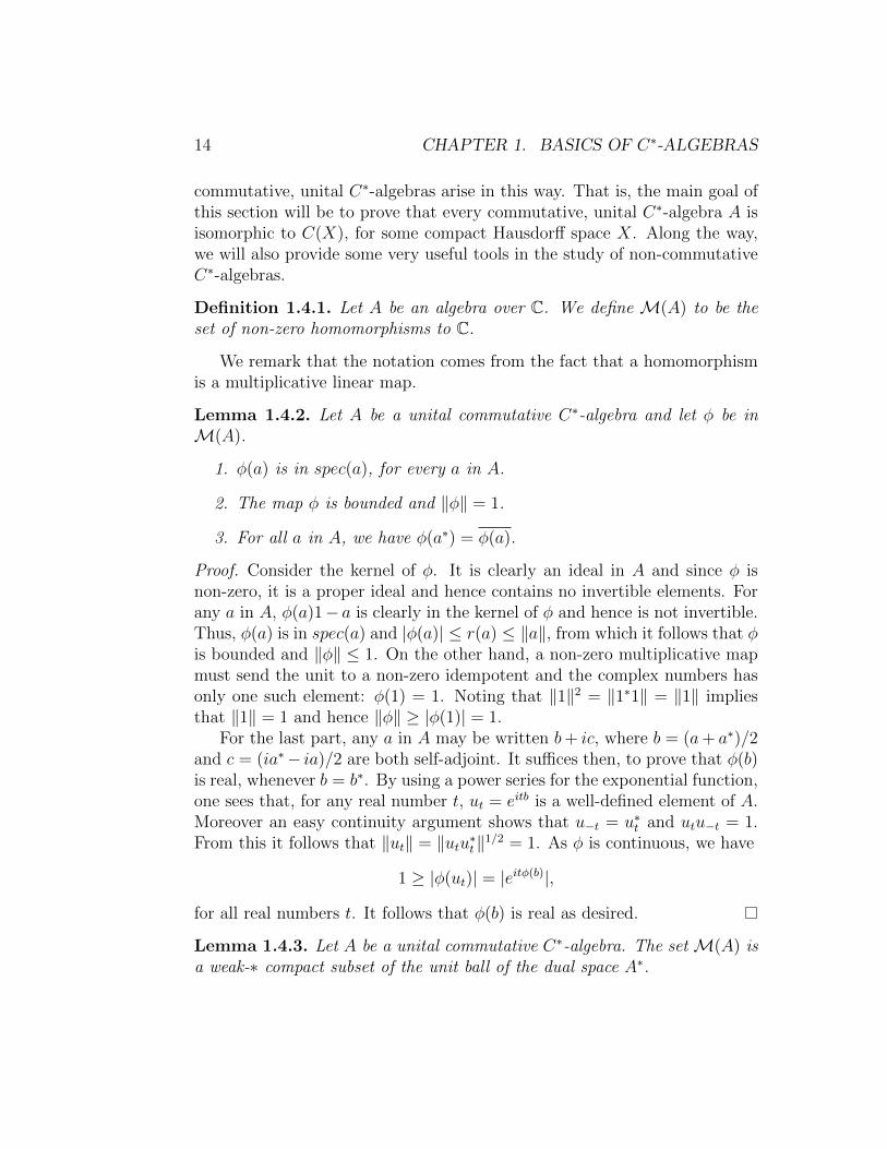
Definition 1.4.1. Let A be an algebra over C. We define M(A) to be theset of non-zero homomorphisms to C.
We remark that the notation comes from the fact that a homomorphismis a multiplicative linear map.
Lemma 1.4.2. Let A be a unital commutative C∗-algebra and let φ be inM(A).
1. φ(a) is in spec(a), for every a in A.
2. The map φ is bounded and ‖φ‖ = 1.
3. For all a in A, we have φ(a∗) = φ(a).
Proof. Consider the kernel of φ. It is clearly an ideal in A and since φ isnon-zero, it is a proper ideal and hence contains no invertible elements. Forany a in A, φ(a)1− a is clearly in the kernel of φ and hence is not invertible.Thus, φ(a) is in spec(a) and |φ(a)| ≤ r(a) ≤ ‖a‖, from which it follows that φis bounded and ‖φ‖ ≤ 1. On the other hand, a non-zero multiplicative mapmust send the unit to a non-zero idempotent and the complex numbers hasonly one such element: φ(1) = 1. Noting that ‖1‖2 = ‖1∗1‖ = ‖1‖ impliesthat ‖1‖ = 1 and hence ‖φ‖ ≥ |φ(1)| = 1.
For the last part, any a in A may be written b+ ic, where b = (a+ a∗)/2and c = (ia∗− ia)/2 are both self-adjoint. It suffices then, to prove that φ(b)is real, whenever b = b∗. By using a power series for the exponential function,one sees that, for any real number t, ut = eitb is a well-defined element of A.Moreover an easy continuity argument shows that u−t = u∗t and utu−t = 1.From this it follows that ‖ut‖ = ‖utu∗t‖1/2 = 1. As φ is continuous, we have
1 ≥ |φ(ut)| = |eitφ(b)|,
for all real numbers t. It follows that φ(b) is real as desired.
Lemma 1.4.3. Let A be a unital commutative C∗-algebra. The set M(A) isa weak-∗ compact subset of the unit ball of the dual space A∗.
1.4. COMMUTATIVE C∗-ALGEBRAS 15
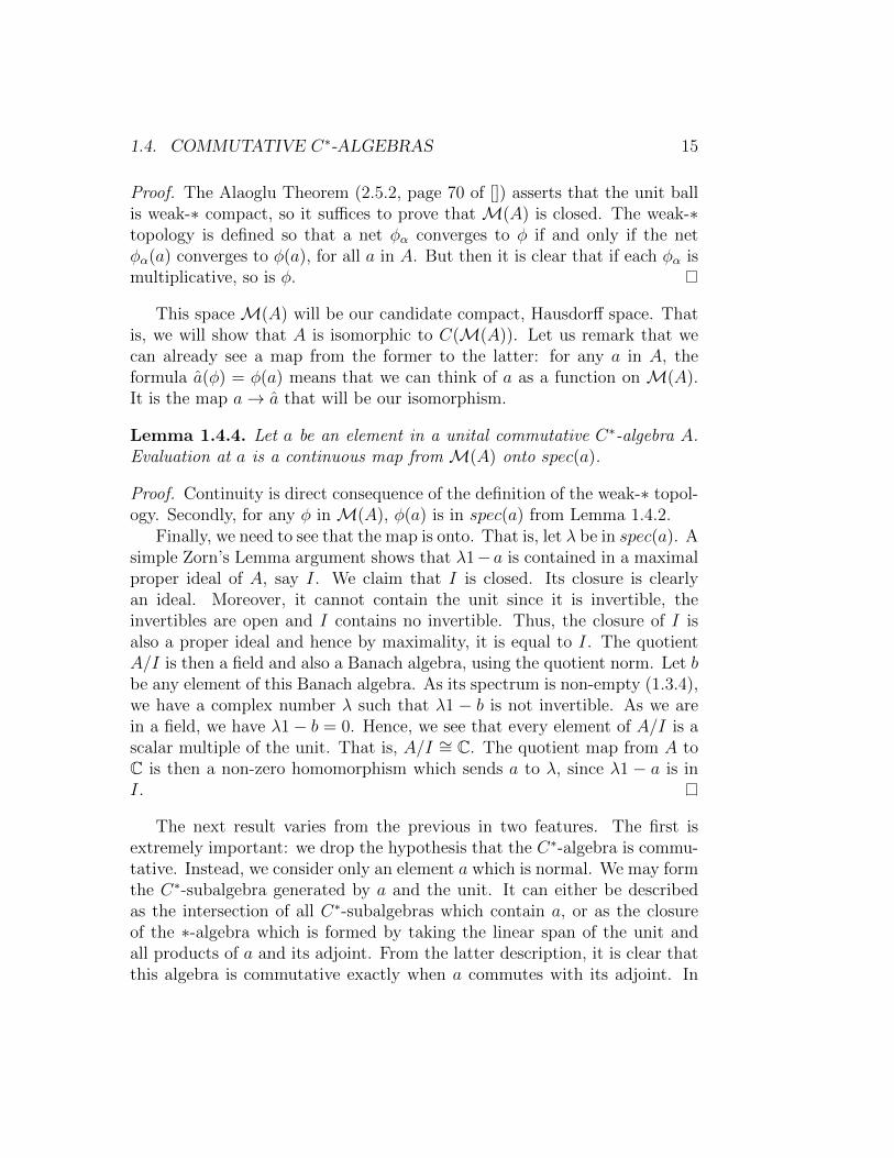
Proof. The Alaoglu Theorem (2.5.2, page 70 of []) asserts that the unit ballis weak-∗ compact, so it suffices to prove that M(A) is closed. The weak-∗topology is defined so that a net φα converges to φ if and only if the netφα(a) converges to φ(a), for all a in A. But then it is clear that if each φα ismultiplicative, so is φ.
This space M(A) will be our candidate compact, Hausdorff space. Thatis, we will show that A is isomorphic to C(M(A)). Let us remark that wecan already see a map from the former to the latter: for any a in A, theformula a(φ) = φ(a) means that we can think of a as a function on M(A).It is the map a→ a that will be our isomorphism.
Lemma 1.4.4. Let a be an element in a unital commutative C∗-algebra A.Evaluation at a is a continuous map from M(A) onto spec(a).
Proof. Continuity is direct consequence of the definition of the weak-∗ topol-ogy. Secondly, for any φ in M(A), φ(a) is in spec(a) from Lemma 1.4.2.
Finally, we need to see that the map is onto. That is, let λ be in spec(a). Asimple Zorn’s Lemma argument shows that λ1−a is contained in a maximalproper ideal of A, say I. We claim that I is closed. Its closure is clearlyan ideal. Moreover, it cannot contain the unit since it is invertible, theinvertibles are open and I contains no invertible. Thus, the closure of I isalso a proper ideal and hence by maximality, it is equal to I. The quotientA/I is then a field and also a Banach algebra, using the quotient norm. Let bbe any element of this Banach algebra. As its spectrum is non-empty (1.3.4),we have a complex number λ such that λ1 − b is not invertible. As we arein a field, we have λ1− b = 0. Hence, we see that every element of A/I is ascalar multiple of the unit. That is, A/I ∼= C. The quotient map from A toC is then a non-zero homomorphism which sends a to λ, since λ1 − a is inI.
The next result varies from the previous in two features. The first isextremely important: we drop the hypothesis that the C∗-algebra is commu-tative. Instead, we consider only an element a which is normal. We may formthe C∗-subalgebra generated by a and the unit. It can either be describedas the intersection of all C∗-subalgebras which contain a, or as the closureof the ∗-algebra which is formed by taking the linear span of the unit andall products of a and its adjoint. From the latter description, it is clear thatthis algebra is commutative exactly when a commutes with its adjoint. In
16 CHAPTER 1. BASICS OF C∗-ALGEBRAS
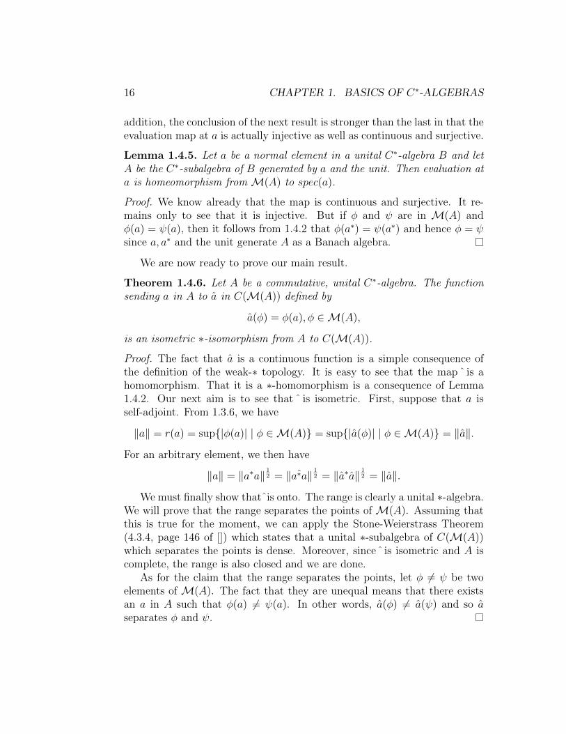
addition, the conclusion of the next result is stronger than the last in that theevaluation map at a is actually injective as well as continuous and surjective.
Lemma 1.4.5. Let a be a normal element in a unital C∗-algebra B and letA be the C∗-subalgebra of B generated by a and the unit. Then evaluation ata is homeomorphism from M(A) to spec(a).
Proof. We know already that the map is continuous and surjective. It re-mains only to see that it is injective. But if φ and ψ are in M(A) andφ(a) = ψ(a), then it follows from 1.4.2 that φ(a∗) = ψ(a∗) and hence φ = ψsince a, a∗ and the unit generate A as a Banach algebra.
We are now ready to prove our main result.
Theorem 1.4.6. Let A be a commutative, unital C∗-algebra. The functionsending a in A to a in C(M(A)) defined by
a(φ) = φ(a), φ ∈M(A),
is an isometric ∗-isomorphism from A to C(M(A)).
Proof. The fact that a is a continuous function is a simple consequence ofthe definition of the weak-∗ topology. It is easy to see that the map ˆ is ahomomorphism. That it is a ∗-homomorphism is a consequence of Lemma1.4.2. Our next aim is to see that ˆ is isometric. First, suppose that a isself-adjoint. From 1.3.6, we have
‖a‖ = r(a) = sup{|φ(a)| | φ ∈M(A)} = sup{|a(φ)| | φ ∈M(A)} = ‖a‖.
For an arbitrary element, we then have
‖a‖ = ‖a∗a‖12 = ‖ ˆa∗a‖
12 = ‖a∗a‖
12 = ‖a‖.
We must finally show thatˆis onto. The range is clearly a unital ∗-algebra.We will prove that the range separates the points of M(A). Assuming thatthis is true for the moment, we can apply the Stone-Weierstrass Theorem(4.3.4, page 146 of []) which states that a unital ∗-subalgebra of C(M(A))which separates the points is dense. Moreover, sinceˆ is isometric and A iscomplete, the range is also closed and we are done.
As for the claim that the range separates the points, let φ 6= ψ be twoelements of M(A). The fact that they are unequal means that there existsan a in A such that φ(a) 6= ψ(a). In other words, a(φ) 6= a(ψ) and so aseparates φ and ψ.
1.4. COMMUTATIVE C∗-ALGEBRAS 17
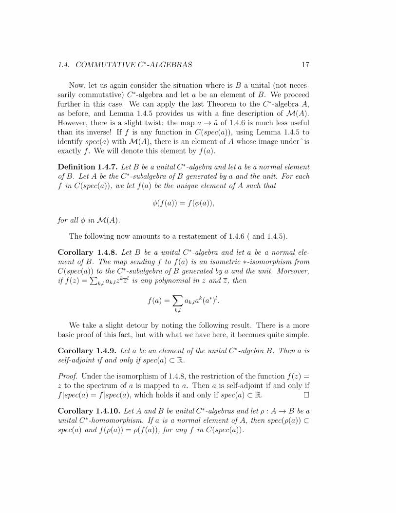
Now, let us again consider the situation where is B a unital (not neces-sarily commutative) C∗-algebra and let a be an element of B. We proceedfurther in this case. We can apply the last Theorem to the C∗-algebra A,as before, and Lemma 1.4.5 provides us with a fine description of M(A).However, there is a slight twist: the map a → a of 1.4.6 is much less usefulthan its inverse! If f is any function in C(spec(a)), using Lemma 1.4.5 toidentify spec(a) withM(A), there is an element of A whose image underˆisexactly f . We will denote this element by f(a).
Definition 1.4.7. Let B be a unital C∗-algebra and let a be a normal elementof B. Let A be the C∗-subalgebra of B generated by a and the unit. For eachf in C(spec(a)), we let f(a) be the unique element of A such that
φ(f(a)) = f(φ(a)),
for all φ in M(A).
The following now amounts to a restatement of 1.4.6 ( and 1.4.5).
Corollary 1.4.8. Let B be a unital C∗-algebra and let a be a normal ele-ment of B. The map sending f to f(a) is an isometric ∗-isomorphism fromC(spec(a)) to the C∗-subalgebra of B generated by a and the unit. Moreover,if f(z) =
∑k,l ak,lz
kzl is any polynomial in z and z, then
f(a) =∑k,l
ak,lak(a∗)l.
We take a slight detour by noting the following result. There is a morebasic proof of this fact, but with what we have here, it becomes quite simple.
Corollary 1.4.9. Let a be an element of the unital C∗-algebra B. Then a isself-adjoint if and only if spec(a) ⊂ R.
Proof. Under the isomorphism of 1.4.8, the restriction of the function f(z) =z to the spectrum of a is mapped to a. Then a is self-adjoint if and only iff |spec(a) = f |spec(a), which holds if and only if spec(a) ⊂ R.
Corollary 1.4.10. Let A and B be unital C∗-algebras and let ρ : A→ B be aunital C∗-homomorphism. If a is a normal element of A, then spec(ρ(a)) ⊂spec(a) and f(ρ(a)) = ρ(f(a)), for any f in C(spec(a)).
18 CHAPTER 1. BASICS OF C∗-ALGEBRAS
Proof. As we observed earlier, it is clear that ρ must carry invertible elementsto invertible elements and the containment follows at once.
For the second part, let C and D denote the C∗-subalgebras of A andB which are generated by a and the unit if A and ρ(a) and the unit of B,respectively. It is clear then that ρ|C : C → D is a unital ∗-homomorphism.Suppose that ψ is in M(D). Then ψ ◦ ρ is in M(C) and we have
ψ(ρ(f(a))) = ψ ◦ ρ(f(a)) = f(ψ ◦ ρ(a)) = f(ψ(ρ(a))).
By definition, this means that ρ(f(a)) = f(ρ(a)).
Exercise 1.4.1. Let X be a compact Hausdorff space. For each x in X,define φx(f) = f(x). Prove that φx is in M(C(X)) and that x → φx is ahomeomorphism between X and M(C(X)). (Hint to show φ is surjective:the Reisz representation theorem identifies the linear functionals on C(X)for you. You just need to identify which are multiplicative.)
Exercise 1.4.2. Suppose that X and Y are compact Hausdorff spaces andρ : C(X)→ C(Y ) is a unital ∗-homomorphism.
1. Prove that there exists a continuous function h : Y → X such thatρ(f) = f ◦ h, for all f in C(X).
2. Prove that this statement may be false if ρ is not unital.
3. Give a necessary and sufficient condition on h for ρ to be injective.
4. Give a necessary and sufficient condition on h for ρ to be surjective.
Exercise 1.4.3. Let B be the C∗-algebra of bounded Borel functions on [0, 1](with the supremum norm). Let Q = {k2−n | k ∈ Z, n ≥ 0} ∩ [0, 1).
1. Let A be the linear span of all functions of the form χ[s,t), χ[t,1], wheres, t are in Q. Prove that A is a ∗-algebra.
2. Let A be the closure of A is the supremum norm, which is a C∗-algebra.Prove that A contains C[0, 1].
3. Prove that for all f in A and s in Q,
limx→s+
f(x), limx→s−
f(x)
both exist.
1.5. FURTHER CONSEQUENCES OF THE C∗-CONDITION 19
4. Let h : M(A) → [0, 1] be the map given in the last exercise and theinclusion C[0, 1] ⊂ A. Describe M(A) and h.
Exercise 1.4.4. Let B be a unital C∗-algebra and suppose a is a self-adjointelement and 1
4> ε > 0 such that ‖a− a2‖ < ε.
1. Let f(x) = x− x2. Prove that
|f(x)| ≥ min
{|x|2,|1− x|
2
},
for all x in R.
2. Prove that spec(a) ⊂ [−2ε, 2ε] ∪ [1− 2ε, 1 + 2ε].
3. Find a continuous function g on spec(a) with values in {0, 1} such that|g(x)− x| < 2ε, for all x in spec(a). Also explain why there is no suchfunction if spec(a) is replaced by [0, 1].
4. Prove that there is a projection p in B such that ‖a− p‖ < 2ε.
1.5 Further consequences of the C∗-condition
In this section, we will prove three more important results on the structureof C∗-algebras.
The first is a nice and somewhat surprising extension of our earlier resultthat any ∗-homomorphism between C∗-algebras is necessarily a contraction(Corollary 1.3.7). If we additionally assume the map is injective, then it isactually isometric.
Lemma 1.5.1. Let A and B be unital C∗-algebras and ρ : A → B be aninjective, unital ∗-homomorphism. Then for any normal element a in A, wehave spec(a) = spec(ρ(a)).
Proof. As ρ maps invertible elements to invertible elements, it is clear thatspec(ρ(a)) ⊂ spec(a).
Let us suppose that the containment spec(ρ(a)) ⊂ spec(a) is proper.Then we may find a non-zero continuous function f defined on spec(a) whoserestriction to spec(ρ(a)) is zero. Then we have f(a) 6= 0 while, using Corol-lary 1.4.8, we have
ρ(f(a)) = f(ρ(a)) = 0
20 CHAPTER 1. BASICS OF C∗-ALGEBRAS
since f |spec(ρ(a)) = 0. This contradicts the hypothesis that ρ is injective.
Theorem 1.5.2. If A and B are unital C∗-algebras and ρ : A → B is aninjective ∗-homomorphism, then ρ is an isometry; that is, ‖ρ(a)‖ = ‖a‖, forall a in A.
Proof. The equality ‖ρ(a)‖ = ‖a‖ for a self-adjoint element a follows fromTheorem 1.3.6 and Lemma 1.5.1. For arbitrary a, we have
‖a‖2 = ‖a∗a‖ = ‖ρ(a∗a)‖ = ‖ρ(a)∗ρ(a)‖ = ‖ρ(a)‖2
and we are done.
Earlier, we defined the spectrum of an element of an algebra. The factthat the definition depends on the algebra in question is implicit. As a verysimple example, the function f(x) = x2 + 1 is invertible when considered inthe ring of continuous functions on the unit interval, C[0, 1], but not as anelement of the ring of polynomials, C[x]. Rather surprisingly, this does notoccur in C∗-algebras. More precisely, we have the following.
Theorem 1.5.3. Let B be a unital C∗-algebra and let A be a C∗-subalgebraof B containing its unit. If a is any element of A, then its spectrum in Bcoincides with its spectrum in A.
Proof. It suffices to show that if a is any element of A which has an inversein B, then that inverse actually lies in A. In the case that a is normal, thisfollows from Lemma 1.5.1 applied to the inclusion map of A in B.
For arbitrary a, if a is invertible, then so is a∗ (its inverse is (a−1)∗) andhence a∗a is also invertible. As a∗a is self-adjoint and hence normal andsince it clearly lies in A, (a∗a)−1 also lies in A. Then we observe a−1 =(a∗a)−1(a∗a)a−1 = (a∗a)−1a∗ which obviously lies in A.
The property of the conclusion of this last theorem is usually called spec-tral permanence.
There is a simple, but useful consequence of this fact and Theorem 1.4.8,usually known as the Spectral Mapping Theorem.
Corollary 1.5.4. Let a be a normal element of a unital C∗-algebra B. Forany continuous function f on spec(a), we have spec(f(a)) = f(spec(a)).That is, the spectrum of f(a) is simply the range of f .
1.6. POSITIVITY 21
Proof. We have already noted the fact that for any compact Hausdorff spaceX and for any f in C(X), the spectrum of f is simply the range of f , f(X).We apply this to the special case of f in C(spec(a)) to see that the spectrum off is f(spec(a)). Since the map from C(spec(a)) to the C∗-algebra generatedby a is an isomorphism and it carries f to f(a) (by definition), we see thatspec(f) = spec(f(a)). The conclusion follows from the fact that the spectrumof a is the same in the C∗-algebra B as it is in the C∗-subalgebra.
Exercise 1.5.1. Show that Theorem 1.5.3 is false if A and B are simplyalgebras over C. In fact, find a maximal counter-example: A ⊂ B suchthat for every element a of A (which is not a multiple of the identity), itsspectrum in A is as different as possible from its spectrum in B.
1.6 Positivity
Let us begin by recalling two things. The first is the definition of a positiveelement in a C∗-algebra given in 1.1.3: an element a in a C∗-algebra is positiveif a = b∗b, for some b in A. Observe that this means that a is necessarilyself-adjoint. Secondly, we recall Corollary 1.4.9: a normal element a of aunital C∗-algebra is self-adjoint if and only if spec(a) ⊂ R. Our goal nowis to provide a similar “spectral” characterization of positivity for normalelements.
Our main result (Theorem 1.6.5) states that a self-adjoint element a in aunital C∗-algebra is positive if and only if spec(a) ⊂ [0,∞). Along the way,we will prove a number of useful facts about positive elements in a unitalC∗-algebra.
Lemma 1.6.1. Let a be a self-adjoint element of a unital C∗-algebra A.
1. Let f(x) = max{x, 0} and g(x) = max{−x, 0}, for x in R. Thenf(a), g(a) are both positive. We have
a = f(a)− g(a),
af(a) = f(a)2,
ag(a) = −g(a)2,
f(a)g(a) = 0.
2. If spec(a) ⊂ [0,∞), then a is positive.
22 CHAPTER 1. BASICS OF C∗-ALGEBRAS
Proof. It is clear that f and g are continuous functions on the spectrum ofa, each is real-valued, f(x) − g(x) = x, xf(x) = f(x)2, xg(x) = −g(x)2 andf(x)g(x) = 0,, for all x in R. Corollary 1.4.8 then implies that f(a), g(a)are self-adjoint elements of A, satisfying the desired equations. Since f(x)is positive, it has a square root and it follows that f(a) = (
√f(a))2 =
(√f(a))∗(
√f(a)) is positive. The same argument shows g(a) is positive.
For the second statement, it suffices to notice in the proof above that ifspec(a) ⊂ [0,∞), then g(a) = 0.
The following statement has a very easy proof which is a nice applicationof the spectral theorem. Moreover, the result is a very useful tool in dealingwith elements with positive spectrum.
Lemma 1.6.2. Let a be a self-adjoint element of a unital C∗-algebra A. Thefollowing are equivalent.
1. spec(a) ⊂ [0,∞).
2. For all t ≥ ‖a‖, we have ‖t− a‖ ≤ t.
3. For some t ≥ ‖a‖, we have ‖t− a‖ ≤ t.
Proof. Since the spectrum of a is a subset of the reals and the spectral radiusof a is its norm, spec(a) ⊂ [−‖a‖, ‖a‖]. We consider the function ft(x) = t−x,for values of t ≥ ‖a‖. The function is positive and monotone decreasing on[−‖a‖, ‖a‖]. Hence, the norm of the restriction of ft to the spectrum of a isjust its value at the infimum of spec(a). In view of Corollary 1.4.8, ‖t−a‖ isalso the value of ft at the infimum of spec(a). Finally, notice that ft(x) ≤ tif and only if x ≥ 0. Putting this together, we see that the minimum ofspec(a) is negative if and only if ‖t − a‖ > t. Taking the negations of bothstatements, spec(a) ⊂ [0,∞) if and only if ‖t − a‖ ≤ t. This holds for allt ≥ ‖a‖.
Here is one very useful consequence of this result.
Proposition 1.6.3. If a and b are self-adjoint elements of the unital C∗-algebra A and spec(a), spec(b) ⊂ [0,∞), then spec(a+ b) ⊂ [0,∞).
1.6. POSITIVITY 23
Proof. Let t = ‖a‖+ ‖b‖ which is evidently at least ‖a+ b‖. Then we have
‖t− (a+ b)‖ = ‖(‖a‖ − a) + (‖b‖ − b)‖≤ ‖(‖a‖ − a)‖+ ‖(‖b‖ − b)‖≤ ‖a‖+ ‖b‖= t,
where we have used the last lemma in moving from the second line to thethird. The conclusion follows from another application of the last lemma.
Before getting to our main result, we will need the following very basicfact regarding the spectrum.
Lemma 1.6.4. Let a, b be two elements of a unital algebra A. Then we have
spec(ab) \ {0} = spec(ba) \ {0}.
Proof. It clearly suffices to prove that if λ is a non-zero complex numbersuch that λ − ab is invertible, then λ − ba is invertible also. Consider x =λ−1 + λ−1b(λ− ab)−1a. We see that
x(λ− ba) = (λ−1 + λ−1b(λ− ab)−1a)(λ− ba)
= 1− λ−1ba+ λ−1b(λ− ab)−1(λa− aba)
= 1− λ−1ba+ λ−1b(λ− ab)−1(λ− ab)a= 1− λ−1ba+ λ−1ba
= 1.
A similar computation which we omit shows that (λ− ba)x = 1 and we aredone.
We are now ready to prove our main result.
Theorem 1.6.5. Let a be a self-adjoint element of a unital C∗-algebra A.Then a is positive if and only if spec(a) ⊂ [0,∞).
Proof. The ’if’ direction has already been done in Lemma 1.6.1. Let us nowassume that a = b∗b, for some b in A. Using the notation of 1.6.1, considerc = bg(a). Then we have c∗c = g(a)b∗bg(a) = g(a)ag(a) = −g(a)3. Write
24 CHAPTER 1. BASICS OF C∗-ALGEBRAS
c = d + ie, where d, e are self-adjoint elements of A. A simple computationshows that
cc∗ = d2 + e2 − c∗c = d2 + e2 + g(a)3.
As the functions x2 and g(x)3 are positive, it follows from Corollary 1.5.4that each of d2, c2 and g(a)3 has spectrum contained in [0,∞). By Lemma1.6.3, so does cc∗. On the other hand, again using Corollary 1.5.4, we havespec(c∗c) = spec(−g(a)3) ⊂ (−∞, 0].
We now appeal to Lemma 1.6.4 (using a = c, b = c∗) to conclude thatspec(c∗c) = spec(cc∗) = {0}. But this means that −g(a)3 = c∗c = 0 and itfollows that g(a) = 0. This implies that the restriction of g to the spectrumof a is zero, which means spec(a) ⊂ [0,∞) and we are done.
It is worth mentioning the following rather handy consequence.
Corollary 1.6.6. If a is a normal element in a unital C∗-algebra B and fis a real-valued function on spec(a), then f(a) is self-adjoint. Similarly, if fis positive, then f(a) is positive.
Proof. We know that spec(f(a)) = f(spec(a)) from Theorem 1.5.4. More-over, since f(a) lies in the C∗-algebra generated by a and the unit, whichis commutative, it itself is normal. The two statements now follow fromCorollary 1.4.9 and Corollary 1.6.5.
Exercise 1.6.1. Let A be a unital C∗-algebra and suppose a is in A. Letf(x) =
√x, x ≥ 0 and define |a| = f(a∗a).
1. Show that if a is invertible, so is |a|.
2. Show that if a is invertible, then u = a|a|−1 is unitary.
3. Prove that if a is invertible, u and |a| commute if and only if a isnormal.
The expression a = u|a| is usually called the polar decomposition of a.
1.7 Finite-dimensional C∗-algebras
In this section, we investigate the structure of finite-dimensional C∗-algebras.The main objective will be the proof of the following theorem, which is a verysatisfactory one.
1.7. FINITE-DIMENSIONAL C∗-ALGEBRAS 25
Theorem 1.7.1. Let A be a unital, finite-dimensional C∗-algebra. Thenthere exist positive integers K and N1, . . . , NK such that
A ∼= ⊕Kk=1MNk(C).
Moreover, K is unique and N1, . . . , NK are unique, up to a permutation.
The theorem is also valid without the hypothesis of the C∗-algebra beingunital (in fact, every finite dimensional C∗-algebra is unital, as a consequenceof the theorem), but we do not quite have the means to prove that yet, sowe content ourselves with the version stated above.
At this point, the reader has a choice. The first option is to simply acceptthe result above as a complete classification of finite-dimensional C∗-algebrasand then move on to the next section. The other option, obviously, is to keepreading to the completion of the section and see the proof. This brings upthe question: is it worth it? Aside from the simple satisfaction of havingseen a complete proof, there are two points in what follows which should bedrawn to the reader’s attention.
The first point is some simple calculus for rank-one operators on Hilbertspace. This is not particularly deep, but the notation is useful and somesimple facts will be assembled which will be used again later, beyond thefinite-dimensional case.
The second point is that the proof of the main result is built aroundthe existence of projections in a finite-dimensional C∗-algebra. In general,C∗-algebras may or may not have non-trivial projections. As an example,C(X), where X is a compact Hausdorff space, has no projections other than0 and 1 if and only if X is connected. However, the principle which is worthobserving is that an abundance of projections in a C∗-algebra can be a greathelp in understanding its structure.
Before we get to a proof of this, we will introduce some useful generalnotation for certain operators on Hilbert space.
Definition 1.7.2. If H is a Hilbert space and ξ, η are vectors in H, then wedefine ξ ⊗ η∗ : H → H by
ξ ⊗ η∗(ζ) =< ζ, η > ξ, ζ ∈ H.
It is worth noting that if H is just CN , for some positive integer N , thenwe can make use of the fact that the matrix product of an i× j matrix and a
26 CHAPTER 1. BASICS OF C∗-ALGEBRAS
j×k matrix exists. With this in mind, if ξ and η are in CN , which we regardas N × 1 matrices, then ξTη is a 1× 1 matrix while ξηT is an N ×N matrix.(Here ξT denotes the transpose of ξ.) The formula above just encodes thesimple consequence of associativity
(ξηT )ζ = ξ(ηT ζ).
Lemma 1.7.3. Let ξ, η, ζ, ω be vectors in the Hilbert space H and let a be inB(H). We have
1. ξ ⊗ η∗ is a bounded linear operator on H and ‖ξ ⊗ η∗‖ = ‖ξ‖‖η‖.
2. (ξ ⊗ η∗)H = span{ξ}, provided η 6= 0.
3. (ξ ⊗ η∗)∗ = η ⊗ ξ∗,
4. (ξ ⊗ η∗)(ζ ⊗ ω∗) =< ζ, η > ξ ⊗ ω∗,
5. a(ξ ⊗ η∗) = (aξ)⊗ η∗,
6. (ξ ⊗ η∗)a = ξ ⊗ (a∗η)∗.
Moreover, if ξ1, ξ2, . . . , ξn is an orthonormal basis for H, then
n∑i=1
aξi ⊗ ξ∗i = a,
for any a in B(H). In particular, the linear span of {ξi ⊗ ξ∗j | 1 ≤ i, j ≤ n}is B(H) and
n∑i=1
ξi ⊗ ξ∗i = 1.
We start toward a proof of the main theorem above by assembling somebasic facts about finite-dimensional C∗-algebras. The main point of the fol-lowing result is that general normal elements can be obtained as linear com-binations of projections.
Lemma 1.7.4. Let A be a unital finite-dimensional C∗-algebra.
1. Every normal element in A has finite spectrum.
2. Every normal element of A is a linear combination of projections.
1.7. FINITE-DIMENSIONAL C∗-ALGEBRAS 27
Proof. For a normal, from 1.4.8, we know that C(spec(a)) is isomorphic toa C∗-subalgebra of A, which must also be finite-dimensional. It follows thatspec(a) is finite.
For each λ in spec(a), let pλ be the element of C(spec(a)) which is 1 onλ and zero elsewhere. As spec(a) is finite, this function is continuous. Asa function, this is clearly a self-adjoint idempotent, so the same is true ofpλ(a). Moreover, it follows that∑
λ∈spec(a)
λpλ(z) = z,
for all z in spec(a). It follows from 1.4.8 that∑λ∈spec(a)
λpλ(a) = a.
Roughly speaking, we now know that a finite-dimensional C∗-algebra hasa wealth of projections. Analyzing the structure of these will be the keypoint in our proof.
Lemma 1.7.5. Let A be a C∗-algebra. The relation defined on projectionsby p ≥ q if pq = q (and hence after taking adjoints qp = q also) is a partialorder.
We leave the proof as an easy exercise.
Lemma 1.7.6. Let A be a C∗-algebra.
1. For projections p, q in A, p ≥ q if and only if pAp ⊃ qAq. In particular,if pAp = qAq, then p = q
2. If pAp has finite dimension greater than 1, then there exists q 6= 0 withp ≥ q.
3. If A is unital and finite-dimensional, then it has minimal non-zeroprojections in the order ≤.
28 CHAPTER 1. BASICS OF C∗-ALGEBRAS
Proof. First, suppose that p ≥ q. Then we have qAq = pqAqp ⊂ pAp.Conversely, suppose that pAp ⊃ qAq. Hence, we have q = qqq ∈ qAq ⊂ pAp,so q = pap, for some a in A. Then pq = ppap = pap = q. For the laststatement, if pAp = qAq, then it follows from the first part that p ≤ q andq ≤ p, hence p = qp = q.
A moment’s thought shows that pAp is a ∗-algebra. It contains ppp = pwhich is clearly a unit for this algebra. If it is finite-dimensional, then it isclosed and hence is a C∗-subalgebra. We claim that if a self-adjoint elementof pAp, say a, has only one point in its spectrum, then that element is a scalarmultiple of p. Let spec(a) = {λ}. Then functions f(z) = z and g(z) = λ areequal on spec(a). So by Corollary 1.4.8, f(a) = g(a). On the other hand,Corollary 1.4.8 also asserts that f(a) = a while g(a) = λp. Our claim followsand this means that if every self-adjoint element of pAp has only one pointin its spectrum that pAp is spanned by p and one dimensional. So if pAp hasdimension greater than one, we must have a self-adjoint element, a, in pApwith at least two points in its spectrum. Choose a surjective function, f ,from spec(a) to {0, 1}. It is automatically continuous on spec(a), q = f(a)is a projection which is non-zero. As q is in pAp, we have pq = q.
For the last statement, we first notice that since A is unital, it containsnon-zero projections. Suppose that p is any non-zero projection in A, sopAp has dimension at least one. If this dimension is strictly greater thanone, we may find q as in part 2. So q is non-zero and since q 6= p, qAq isa proper linear subspace of pAp, so dim(qAq) < dim(pAp). Continuing inthis fashion, we may eventually find q such that dim(qAq) = 1. Hence, q isminimal in the order ≤ among non-zero projections.
We will consider non-zero projections p which are minimal with respectto the relation ≥. From the last result, we have pAp = Cp, for any suchprojection.
Lemma 1.7.7. Suppose that p1, p2, . . . , pK are minimal, non-zero projectionsin A with piApj = 0, for i 6= j. Then p1, . . . , pK are linearly independent.A finite set of minimal projections satisfying the hypothesis will be calledindependent.
Proof. If some pi can be written as a linear combination of the others, then
1.7. FINITE-DIMENSIONAL C∗-ALGEBRAS 29
we would have
Cpi = piApi = piA(∑j 6=i
αjpj) ⊂∑j 6=i
piApj = 0,
a contradiction.
Lemma 1.7.6 guarantees the existence of minimal, non-zero projectionsin a unital, finite-dimensional C∗-algebra A. Lemma 1.7.7 shows that anindependent set of these cannot contain more than dim(A) elements and itfollows that we may take a maximal independent set of minimal, non-zeroprojections and it will be finite.
Theorem 1.7.8. Let A be a finite-dimensional C∗-algebra and letp1, p2, . . . , pK be a maximal set of independent minimal non-zero projectionsin A.
1. For each 1 ≤ k ≤ K, Apk is a finite-dimensional Hilbert space withinner product < a, b > pk = b∗a, for all a, b in Apk.
2. For each 1 ≤ k ≤ K, ApkA (meaning the linear span of elements ofthe form apka
′ with a, a′ in A) is a unital C∗-subalgebra of A.
3. ⊕Kk=1ApkA = A,
4. For each 1 ≤ k ≤ K, define the map πk : A → B(Apk) defined byπk(a)b = ab, for a in A and b in Apk. Then πk is a ∗-homomorphismand its restriction to AplA is zero for l 6= k and an isomorphism forl = k.
Proof. For the first statement, if a, b are in Apk, then a = apk, b = bpk andso b∗a = (bpk)
∗apk = pkb∗apk ∈ pkApk = Cpk, so the scalar < a, b > as
described exists. This is clearly linear in a and conjugate linear in b. It isclearly non-degenerate, for if < a, a >= 0, then a∗a = 0 which implies a = 0.
Choose Bk to be an orthonormal basis for Apk which means that for anya in Apk, we have∑
b∈Bk
bb∗a =∑b∈Bk
b < a, b > pk =∑b∈Bk
< a, b > bpk =∑b∈Bk
< a, b > b = a.
Next, we define
qk =∑b∈Bk
bb∗ =∑b∈Bk
bpkb∗.
30 CHAPTER 1. BASICS OF C∗-ALGEBRAS
It is clear that qk is self-adjoint, in ApkA and, from above, qka = a, for anya in Apk.
Now if a, a′ are in A, we have
qk(apka′) = (qkapk)a
′ = apka′
and(apka
′)qk = (qk(a′)∗pka
∗)∗ = ((a′)∗pka∗)∗ = apka
′,
so that qk is a unit forApkA. This completes the proof of part 2. In particular,we note that qkpk = pk.
Since pkApl = 0 for all k 6= l, we see that ApkA ·AplA = 0 as well. Fromthis, we also see that qkApl = 0 and qkAplA = 0 for k 6= l. In particular, theprojections qk are pairwise orthogonal.
Consider q = 1 −∑K
k=1 qk. It is easily seen that q is a projection andqqk = 0, for all k. If q is non-zero, then it is greater than some minimalprojection p. In this case, we have ppk = pqqkpk = 0, for all k. Thiscontradicts our choice of the pk’s as a maximal independent set of minimalprojections. Thus
∑k qk = 1. We have
A =
(∑k
qk
)A = ⊕Kk=1qkA = ⊕Kk=1ApkA.
Now, we must establish the last part. We know already that AqlA actstrivially on Apk, if l 6= k. The only thing remaining to verify is that πk is anisomorphism from ApkA to B(Apk). Every element of Apk is in the span ofBk. It follows that every element of pkA = (Apk)
∗ is a linear combination thethe adjoints of elements of Bk. Therefore apka
′ = (apk)(a′pk)
∗ is in the spanof bc∗, b, c ∈ Bk. For any scalars αb,c, b, c ∈ Bk and b0, c0 in Bk, we compute
< πk
(∑b,c
αb,cbc∗
)c0, b0 > pk =
∑b,c
αb,c < bc∗c0, b0 > pk =∑b,c
αb,cb∗0bc∗c0.
Since Bk is an orthonormal basis, b∗0b is zero unless b = b0, in which case itis pk. Similarly, c∗c0 is zero unless c = c0, in which case it is also pk. Weconclude that
< πk
(∑b,c
αb,cbc∗
)c0, b0 > pk = αb0,c0pk.
1.7. FINITE-DIMENSIONAL C∗-ALGEBRAS 31
If πk(∑
b,c αb,cbc∗) = 0, it follows that each coefficient αb,c is zero and from
this it follows that the restriction of πk to ApkA is injective.We now show πk is onto. Let a, b be in Apk. We claim that πk(ab
∗) =a⊗ b∗. For any c in Apk, we have
(a⊗ b∗)c =< c, b > a =< c, b > apk = a(< c, b > pk) = a(b∗c) = πk(ab∗)c.
We have shown that the rank one operator a ⊗ b∗ is in the range of πk andsince the span of such operators is all of B(Apk), we are done.
Theorem 1.7.9. If N is a positive integer, then the centre of MN(C) is thescalar multiples of the identity. If N1, N2, . . . , NK are positive integers, thenthe centre ⊕Kk=1MNk(C) is isomorphic to CK and is spanned by the identityelements of the summands.
Proof. We may assume thatN ≥ 2, since the other case is trivial. We identifyMN(C) and B(CN). Suppose that a is in the centre of B(CN) and let ξ beany vector in CN . Then we have
(aξ ⊗ ξ∗) = a(ξ ⊗ ξ∗) = (ξ ⊗ ξ∗)a = ξ ⊗ (a∗ξ)∗.
Applying both sides to the vector ξ, we see that
aξ < ξ, ξ >=< a∗ξ, ξ > ξ.
It follows that, for every vector ξ there is a scalar r such that aξ = rξ. If ξand η are two linearly independent vectors we know that there are scalars,r, s, t, such that
r(ξ + η) = a(ξ + η) = aξ + aη = sξ + tη.
By linear independence, we see that r = s = t. We have shown that for everyvector ξ, aξ is a scalar multiple of ξ. Moreover, the scalar is independent ofξ. Thus a is a multiple of the identity.
The second statement follows immediately from the first.
Let us complete the proof of Theorem 1.7.1. In fact, almost everythingis done. We know that from part 3 of Theorem 1.7.8 that A = ⊕kApkA andfrom part 4 of the same theorem that, for each k, πk : ApkA→ B(Apk) is anisomorphism. Therefore, we have
⊕Kk=1πk : A = ⊕Kk=1ApkA→ ⊕Kk=1B(Apk)
32 CHAPTER 1. BASICS OF C∗-ALGEBRAS
is an isomorphism.It only remains for us to prove the uniqueness of K and N1, N2, . . . , NK .
We see from the last result that K is equal to the dimension of the centre ofA. Next, the units of the summands of A are exactly the minimal non-zeroprojections in the centre and if qk is the unit of summand MNk , then Nk isthe square root of the dimension of qkA.
Exercise 1.7.1. Let A be a unital C∗-algebra. Let e be in A and satisfy e∗eis a projection. Prove that
1. ee∗e = e. (Hint: compute (ee∗e− e)∗(ee∗e− e).)
2. ee∗ is also a projection.
Exercise 1.7.2. Let A be a C∗-algebra and let n ≥ 1. Suppose that we haveelements of A, ei,j, 1 ≤ i, j ≤ n which satisfy
ei,jek,l =
{ei,l j = k0 j 6= k
and e∗i,j = ej,i, for all i, j, k, l. Assuming that at least one ei,j is non-zero,prove that the span of the ei,j, 1 ≤ i, j,≤ n, is a C∗-subalgebra of A and isisomorphic to Mn(C). (Hint: first show that all ei,j are non-zero, then showthey are linearly independent.) Such a collection of elements is usually calleda set of matrix units.
Exercise 1.7.3. Suppose that a1, a2, . . . , aN are elements in a C∗-algebra Aand satisfy:
1. a∗1a1 = a∗2a2 = · · · = a∗NaN is a projection,
2. aia∗i aja
∗j = 0 for all 1 ≤ i 6= j ≤ N .
Prove that ei,j = aia∗j , 1 ≤ i, j ≤ N is a set of matrix units.
1.8 Non-unital C∗-algebras
The main result in this section establishes a very close connection betweennon-unital and unital C∗-algebras.
1.8. NON-UNITAL C∗-ALGEBRAS 33
Theorem 1.8.1. Let A be a C∗-algebra. There exists a C∗-algebra A whichis unital, contains A as a closed two-sided ideal and A/A ∼= C. Moreover,this C∗-algebra is unique.
Proof. Let A = C⊕ A, as a vector space. We define the product on A by
(λ, a)(µ, b) = (λµ, λb+ µa+ ab),
for a, b in A and λ, µ in C. We also define
(λ, a)∗ = (λ, a∗),
for a in A and λ in C. It is clear that (1, 0) is a unit for this algebra. Themap sending a in A to (0, a) is obviously an injective ∗-homomorphism ofA into A, whose image is an ideal. We will usually suppress this map inour notation; this means that, for a in A, (0, a) and a mean the same thing.Moreover, the quotient of A by A is obviously isomorphic to C.
We turn now to the issue of a norm. In fact, it is quite easy to see thatby defining
‖(λ, a)‖1 = |λ|+ ‖a‖,
for (λ, a) in A, we obtain a Banach algebra with isometric involution. Gettingthe C∗-condition (which does not hold for this norm) is rather trickier.
Toward a definition of a good C∗-norm, let us make a nice little observa-tion. If we recall only the fact that A is a Banach space, we can study B(A),the algebra of bounded linear operators on it. Recalling now the product onA, the formula π(a)b = ab, for a, b in A, defines π(a) as an operator on A.The Banach algebra inequality ‖ab‖ ≤ ‖a‖‖b‖, simultaneously shows thatπ(a) is in B(A) and ‖π(a)‖ ≤ ‖a‖. It is easy to see that π : A → B(A) is ahomomorphism. Finally, we consider
‖π(a)a∗‖ = ‖aa∗‖ = ‖a‖2 = ‖a‖‖a∗‖,
which inplies that ‖π(a)‖ = ‖a‖. In short, the norm on A can be seen as theoperator norm of A acting on itself.
We are going to use a minor variation of that: since A is an ideal in A,we can think of A as acting on A.
We define a norm by
‖(λ, a)‖ = sup{|λ|, ‖(λ, a)b‖, ‖b(λ, a)‖ | b ∈ A, ‖b‖ ≤ 1},
34 CHAPTER 1. BASICS OF C∗-ALGEBRAS
for all (λ, a) in A. Notice that (λ, a)b = λb+ ab is in A so the norm involvedon the right is that of A. It is easy to see the set on the right is bounded(by ‖(λ, a)‖1), so the supremum exists. We claim that ‖(0, a)‖ = ‖a‖, forall a in A. The inequality ≤ follows from the fact that the norm on A is aBanach algebra norm. Letting b = ‖a‖−1a∗ yields the inequality ≥ (at leastfor non-zero a).
We next observe that ‖(λ, a)‖ = 0 implies (using b = ‖a‖−1a∗) that|λ| = ‖aa∗‖ = 0 which in turn means that (λ, a) = (0, 0). It is easy to seethat ∗ is isometric. Next, it is trivial that ‖(λ, a)‖ ≤ |λ|+‖a‖ and since bothC and A are complete, so is A in this norm. We leave the details that thenorm satisfies the Banach space conditions to the reader.
This leaves us to verify the C∗-condition. Let (λ, a) be in A. The inequal-ity ‖(λ, a)∗(λ, a)‖ ≤ ‖(λ, a)‖2 follows from the Banach property and that ∗ isisometric. For the reverse, we first note that note that ‖(λ, a)∗(λ, a)‖ ≥ |λ|2.Next, for any b in the unit ball of A, we have
‖(λ, a)∗(λ, a)b‖ ≥ ‖b∗‖‖(λ, a)∗(λ, a)b‖≥ ‖b∗(λ, a)∗(λ, a)b‖= ‖(λ, a)b‖2.
Taking the supremum over all b in the unit ball yields ‖(λ, a)∗(λ, a)‖ ≥‖(λ, a)‖2.
The last item is to prove the uniqueness of A. Suppose that B satisfiesthe desired conditions. We define a map from A as above to B by ρ(λ, a) =λ1B + a, for all λ ∈ C and a ∈ A. It is a simple computation to seethat ρ is a ∗-homomorphism. Let q : B → B/A be the quotient map.Since A is an ideal and is not all of B, it cannot contain the unit of B.Thus q(1B) 6= 0. Let us prove that ρ is injective. If ρ(λ, a) = 0, then0 = q ◦ ρ(λ, a) = q(λ1B + a) = λq(1B) and we conclude that λ = 0. Itfollows immediately that a = 0 as well and so ρ is injective. It is clear thatA is contained in the image of ρ and that q ◦ ρ is surjective as well. SinceB/A is one-dimensional, we conclude that ρ is surjective. The fact that ρ isisometric follows from Theorem 1.5.2.
We conclude with a few remarks concerning the spectral theorem in thecase of non-unital C∗-algebras. Particularly, we would like generalizations ofTheorem 1.4.6 amd Corollary 1.4.8. To generalize Theorem 1.4.6, we wouldsimply like to drop the hypothesis that the algebra be unital.
1.8. NON-UNITAL C∗-ALGEBRAS 35
Before beginning, let us make a small remark. If x0 is a point in somecompact Hausdorff space X, there is a natural isomorphism {f ∈ C(X) |f(x0) = 0} ∼= C0(X \ {x0}) which simply restricts the function to X \ {x0}.
Theorem 1.8.2. Let A be a C∗-algebra, let A be as in Theorem 1.8.1 andlet π : A → C be the quotient map with kernel A. Then π is in M(A).Moreover, the restriction of the isomorphism of 1.4.6 to A is an isometric∗-isomorphism between A and C0(M(A) \ {π}).
Proof. We give a sketch only. The first statement is clear. Secondly, ifa is in A, then a(π) = π(a) = 0, by definition of π. So ˆ maps A intoC0(M(A) \ {π}) (using the indentification above) and is obviously an iso-metric ∗-homomorphism. The fact that it is onto follows from the facts thatA has codimension one in A while the same is true of C0(M(A) \ {π}) inC(M(A)).
We note the obvious corollary.
Corollary 1.8.3. If A is a commutative C∗-algebra then there exists a locallycompact Hausdorff space X such that A ∼= C0(X). Moreover, X is compactif and only if A is unital.
Generalizing Corollary 1.4.8 is somewhat more subtle. If a is a normalelement of any (possibly non-unital) C∗-algebra B, we can always replaceB by B and apply 1.4.8. So the hypothesis that B is a unital C∗-algebrais rather harmless. The slight catch is that the isomorphism of 1.4.8 hasrange which is the C∗-subalgebra generated by a and the unit, which takesus outside of our original B, if it is not unital. The appropriate version herestrengthens the conclusion by showing that, for functions f in C(spec(a))satisfying f(0) = 0, f(a) actually lies in the C∗-subalgebra generated bya. This fact is quite useful even in situations where B is unital, since itstrengthens the conclusion of Theorem 1.4.8. This is, in fact, how it is stated.
Theorem 1.8.4. Let a be a normal element of the unital C∗-algebra B.The isomorphism of 1.4.8 restricts to an isometric ∗-isomorphism betweenC0(spec(a) \ {0}) and the C∗-subalgebra of B generated by a.
Proof. Again, we provide a sketch. First, assume that 0 is not in the spectrumof a, so a is invertible. Notice that C0(spec(a)\{0}) = C(spec(a)). We wouldlike to simply apply 1.4.8, but we need to see that the C∗-algebra generated
36 CHAPTER 1. BASICS OF C∗-ALGEBRAS
by a and the unit is the same as that generated by a alone. Now, let f bethe continuous function on spec(a) ∪ {0} which is 1 on spec(a) and 0 at 0.Let ε > 0 be arbitrary and use Weierstrass’ Theorem to approximate f by apolynomial p(z, z) to within ε. It follows that p(z, z)−p(0, 0) is a polynomialwith no constant term which approximates f to within 2ε. Then p(a, a∗)is within 2ε of f(a) = 1. On the other hand, the formula of 1.4.8 showsthat p(a, a∗) is in the C∗-subalgebra generated by a alone. In this case, theconclusion is exactly the same as for 1.4.8.
Now we assume that 0 is in the spectrum of a. Let f be in C0(spec(a) \{0}). We may view f as a continuous function of spec(a) by defining f(0) = 0.Again let ε > 0 be arbitrary and use Weierstrass’ Theorem to approximatef by a polynomial p(z, z) to within ε. It follows that p(z, z) − p(0, 0) is apolynomial with no constant term which approximates f to within 2ε. Again,we see that f(a) can be approximated to within 2ε by an element of the C∗-algebra generated by a alone. From this we see that C0(spec(a) \ {0}) ismapped to the C∗-subalgebra generated by a. The rest of the conclusion isstraightforward.
Exercise 1.8.1. If A is a unital C∗-algebra, then A ∼= C⊕A as C∗-algebras( see Example 1.2.5). Write the isomorphism explicitly, since it isn’t theobvious one!
Exercise 1.8.2. Let X be a locally compact Hausdorff space and let A =C0(X). Prove that M(A) is homeomorphic to X ∪ {∞}, the one-point com-pactification of X. Discuss the overlap of this exercise and the last one.
1.9 Ideals and quotients
In this section, we consider ideals in a C∗-algebra. Now ideals come in manyforms; they can be either one-sided or two-sided and they may or may not beclosed. We will concentrate here on closed, two-sided ideals. Generally, one-sided ideals are rather difficult to describe. (For a simple tractible case, seeExercise 1.9.2 below.) Ideals that are not closed can be even worse, althoughin specific situations, there are ones of interest that arise. For an example,the set of all finite rank operators in B(H) is an ideal which is not closed. Foranother example, consider a locally compact, non-compact Hausdorff spaceX. The set of all compactly supported continuous functions on X is an idealin C0(X).
1.9. IDEALS AND QUOTIENTS 37
If A is a C∗-algebra and I is a closed subspace, then we may form thequotient space A/I. We remark that the norm on the quotient A/I is definedby
‖a+ I‖ = inf{‖a+ b‖ | b ∈ I}.
For the proofs that this is a well-defined norm and makes A/I into a Banachspace, we refer the reader to [?].
If, in addition, I is also a two-sided ideal, then A/I is also an algebra,just as usual in a first course in ring theory and it is an easy matter to checkthat our norm above is actually a Banach algebra norm. At this point, A/Imight fall short of being a C∗-algebra on two points. The first is having a∗-operation. There is an obvious candidate, (a+ I)∗ = a∗+ I, but to see thisis well-defined, we need to know that I is closed under ∗. The second pointis seeing that the norm satisfies C∗-condition. This all turns out to be trueand we state our main result.
Theorem 1.9.1. Let A be a C∗-algebra and suppose that I is a closed (mean-ing as a topological subset), two-sided ideal. Then I is also closed under the∗-operation and A/I, with the quotient norm, is a C∗-algebra.
In the course of the proof, we will need the following technical result.
Lemma 1.9.2. Let a be an element in a C∗-algebra A. For any ε > 0, thereis a continuous function f on [0,∞) such that e = f(a∗a) is in A, is positive,‖e‖ ≤ 1 and ‖a− ae‖ < ε.
Proof. We note from Theorem 1.13.1 that spec(a∗a) ⊂ [0,∞). Define thefunction f on [0,∞) by f(t) = t(ε + t)−1. Since f(0) = 0, we may applyTheorem 1.7.5 to see that f(a∗a) is contained in the C∗-algebra generatedby a∗a and hence in A. It is clear that 0 < f(t) < 1, for all 0 ≤ t < ∞and so e = f(a∗a) is well-defined, positive and norm less than or equal toone. Notice in what follows, when we write expressions like 1 − e, this canbe regarded as an element of A, even if A is non-unital. We have
‖a− ae‖2 = ‖a(1− e)‖= ‖a(1− f(a∗a))‖2
= ‖(1− f(a∗a))a∗a(1− f(a∗a))‖= ‖g(a∗a)‖≤ ‖g‖∞,
38 CHAPTER 1. BASICS OF C∗-ALGEBRAS
where g(t) = t(1 − f(t))2. It is a simple calculus exercise to check that gattains its maximum (on the positive axis) at t = ε and its maximum isε/4.
We now turn to the proof of the main result.
Proof. Let a be in I. We will show that a∗ is also. Let ε > 0 and applythe last lemma to a. Since a is in I, so is a∗a. We claim that e = f(a∗a) isin I, also. This point is a little subtle in applying 1.7.5 since we do not yetknow that I is a C∗-algebra. However, we are applying the function to theself-adjoint element a∗a. By approximating the function by polynomials ina∗a we see that the C∗-algebra generated by this element is the same as theclosed algebra generated by the element and hence is contained in I.
Since e is self-adjoint and the ∗ operation is isometric, we have
‖a∗ − ea∗‖ = ‖a− ae‖ ≤ ε.
Since e is in I, so is ea∗. We see then that a∗ is within ε of an element of I.As I is closed and ε is arbitrary, we conclude that a∗ is in I.
We now prove that the norm satisfies the C∗-condition.Let a be in A. First, we show that the ∗ operation is isometric since
‖a∗ + I‖ = inf{‖a∗ + b‖ | b ∈ I}= inf{‖a∗ + b∗‖ | b ∈ I}= inf{‖a+ b‖ | b ∈ I}= ‖a+ I‖.
Now it suffices to prove that ‖a+ I‖2 ≤ ‖a∗a+ I‖. We claim that
‖a+ I‖ = inf{‖a+ b‖ | b ∈ I} = inf{‖a(1− e)‖ | e ∈ I, e ≥ 0, ‖e‖ ≤ 1}.
We first observe that any element e satisfying e ≥ 0 (meaning that e ispositive) and norm less than 1 must have spectrum contained in [0, 1]. Itfollows that the norm of 1− e also has norm less than 1.
As a(1−e) = a−ae and ae is in I for any e satisfying the given conditions,we see immediately that
inf{‖a+ b‖ | b ∈ I} ≤ inf{‖a(1− e)‖ | e ∈ I, e ≥ 0, ‖e‖ ≤ 1}.
1.9. IDEALS AND QUOTIENTS 39
For the reverse, let b be in I let ε > 0 and use the Lemma to obtain e asdesired with ‖b− be‖ < ε. Then we have
‖a+ b‖ ≥ ‖(a+ b)(1− e)‖ ≥ ‖a(1− e)‖ − ‖b− be‖ ≥ ‖a(1− e)‖ − ε.As ε > 0 was arbitrary, we have established the reverse inequality.
Having the claim, we now check that for a given e with conditions asabove, we have
‖a(1− e)‖2 = ‖(1− e)a∗a(1− e)‖ ≤ ‖a∗a(1− e)‖.Taking infimum over all such e yields the result.
As a final remark, we note that if I is a closed, two-sided ideal in A,the natural quotient map π(a) = a + I, a ∈ A from A to A/I is a ∗-homomorphism. The proof is a triviality, but this can often be a usefulpoint of view.
Exercise 1.9.1. 1. Let X be a compact, Hausdorff space and let A =C(X). Let Z ⊂ X be closed and
I = {f ∈ C(X) | f(z) = 0, for all z ∈ Z}.First prove that I is a closed, two-sided ideal in A. Next, since I andA/I are both clearly commutative C∗-algebras (although the former maynot be unital) find M(I) and M(A/I).
2. Let A be as above. Prove that any closed two-sided ideal I in A arisesas above. (Hint: A/I is commutative and unital; use Exercise 1.4.2 onthe quotient map.)
Exercise 1.9.2. Let n ≥ 2 and A = Mn(C).
1. Suppose that I is a right ideal in A. Show that ICn = {aξ | a ∈ I, ξ ∈Cn} is a subspace of Cn. (Hint: if ξ, η are unit vectors and a is amatrix, then aξ = a(ξ ⊗ η∗)η.)
2. Prove the correspondence between the set of all right ideals in A andthe set of all linear subspaces of Cn in the previous part is a bijection.
3. Prove that A is simple; that is, it has no closed two-sided ideals except0 and A.
Exercise 1.9.3. Let ρ : A → B be a ∗-homomorphism between two C∗-algebras. Prove that ρ(A) is closed and is a C∗-subalgebra of B. (Hint:Theorem 1.9.1 and Theorem 1.5.2.)
40 CHAPTER 1. BASICS OF C∗-ALGEBRAS
1.10 Traces
As a C∗-algebra is a Banach space, it has a wealth of linear functionals, basi-cally thanks to the Hahn-Banach Theorem. We can ask for extra propertiesin a linear functional. Indeed we did back in Chapter 1.4 when we lookedat homomorphisms which are simply linear functionals which are multiplica-tive. That was an extremely successful idea in dealing with commutativeC∗-algebras, but most C∗-algebras of interest will have none.
It turns out that there is some middle ground between being a linearfunctional and a homomorphism. This is the notion of a trace.
Definition 1.10.1. Let A be a unital C∗-algebra. A linear functional φ onA is said to be positive if φ(a∗a) ≥ 0, for all a in A. A trace on A is apositive linear functional τ : A→ C with τ(1) = 1 satisfying
τ(ab) = τ(ba),
for all a, b in A. This last condition is usually called the trace property. Thetrace is said to be faithful if τ(a∗a) = 0 occurs only for a = 0.
Notice that the trace property is satisfied by any homomorphism, but wewill see that it is strictly weaker. For the moment, it is convenient to regardit as something stronger than mere linearity (or even positivity) but weakerthan being a homomorphism.
Example 1.10.2. If A is commutative, every positive linear functional is atrace.
Theorem 1.10.3. Let H be a Hilbert space of (finite) dimension n. If{ξ1, . . . , ξn} is an orthonormal basis for H, then
τ(a) = n−1
n∑i=1
< aξi, ξi >,
for any a in B(H), defines a faithful trace on B(H). The trace is unique. Ifwe identify B(H) with Mn(C), then this trace is expressed as
τ(a) = n−1
n∑i=1
ai,i
for any a in Mn(C).
1.10. TRACES 41
Proof. First, it is clear that τ is a linear functional. Next, we see that, forany a in B(H), we have
τ(a∗a) = n−1
n∑i=1
< a∗aξi, ξi >= n−1
n∑i=1
< aξi, aξi >= n−1
n∑i=1
‖aξi‖2.
It follows at once that τ is positive. Moreover, if τ(a∗a) = 0, then aξi = 0,for all i. As a is zero on a basis, it is the zero operator. We also see fromthis, using a = 1, that τ(1) = 1.
It remains for us to verify the trace property. We do this by first consid-ering the case of rank one operators. We observe that, for any ξ, η in H, wehave
τ(ξ ⊗ η) = n−1
n∑i=1
< (ξ ⊗ η)ξi, ξi >
= n−1
n∑i=1
< ξi, η >< ξ, ξi >
= n−1 <n∑i=1
< ξ, ξi > ξi, η >
= n−1 < ξ, η > .
Now let ξ, η, ζ, ω be in H and a = ξ ⊗ η∗, b = ζ ⊗ ω∗. We have ab =< ζ, η >ξ⊗ω∗ and ba =< ξ, ω > ζ ⊗ η∗. It follows then from the computation abovethat
τ(ab) = < ζ, η > τ(ξ ⊗ ω∗)= n−1 < ζ, η >< ξ, ω >
= < ξ, ω > τ(ζ ⊗ η∗)= τ(ba).
Since the linear span of such operators is all of B(H), the trace propertyholds.
We finally turn to the uniqueness of the trace. Suppose that φ is anytrace on B(H). We will show that φ and τ agree on ξi ⊗ ξ∗j , first consideringthe case i 6= j. Let a = ξi ⊗ ξ∗i and b = ξi ⊗ ξ∗j . It follows that ab = b whileba = 0. Therefore, we have φ(b) = φ(ab) = φ(ba) = 0 = τ(b). Next, for any
42 CHAPTER 1. BASICS OF C∗-ALGEBRAS
i, j, let v = ξi ⊗ ξ∗j . Then v∗v = ξj ⊗ ξ∗j while vv∗ = ξi ⊗ ξ∗i . Therefore, wehave φ(ξi ⊗ ξ∗i ) = φ(ξj ⊗ ξ∗j ). Finally, we have
1 = φ(1) = φ
(n∑i=1
ξi ⊗ ξ∗i
)= nφ(ξ1 ⊗ ξ∗1).
Putting these together, we see that
φ(ξi ⊗ ξ∗i ) = φ(ξ1 ⊗ ξ∗1) = n−1 = τ(ξi ⊗ ξ∗i ).
We have shown that τ and φ agree on a spanning set, ξi ⊗ ξ∗j , 1 ≤ i, j ≤ n,hence they are equal.
We mention in passing the following handy fact. Basically, it is telling usthat, when applied to projections, the trace recovers the geometric notion ofthe dimension of the range.
Theorem 1.10.4. Let τ be the unique trace on B(H), where H is a finitedimensional Hilbert space. If p is a projection, then dim(pH) = τ(p)dim(H).
Proof. Choose an orthonormal basis {ξ1, . . . , ξn} for H is such a way that{ξ1, . . . , ξk} is a basis for pH. We omit the remaining computation.
Exercise 1.10.1. Prove that, for n > 1, there is no non-zero∗-homomorphism from Mn(C) to C. In fact, give two different proofs, oneusing 1.10.3 above, and one using Exercise 1.9.2.
1.11 Representations
The study of C∗-algebras is motivated by the prime example of closed ∗-algebras of operators on Hilbert space. With this in mind, it is natural tofind ways that a given abstract C∗-algebra may act as operators on Hilbertspace. Such an object is called a representation of the C∗-algebra.
Definition 1.11.1. Let A be a ∗-algebra. A representation of A is a pair,(π,H), where H is a Hilbert space and π : A→ B(H) is a ∗-homomorphism.We also say that π is a representation of A on H.
1.11. REPRESENTATIONS 43
Now the reader should prepare for a long list of simple properties, con-structions and results concerning representations.
The first important notion for representations is that of unitary equiva-lence. One should consider unitarily equivalent representations as being ’thesame’.
Definition 1.11.2. Let A be a ∗-algebra. Two representations of A,(π1,H1), (π2,H2), are unitarily equivalent if there is a unitary operator u :H1 → H2 such that uπ1(a) = π2(a)u, for all a in A. In this case, we write(π1,H1) ∼u (π2,H2) or π1 ∼u π2.
The most important operation on representations of a fixed ∗-algebra isthe direct sum. The following definition is stated in some generality, but atfirst pass, the reader can assume the collection of representations has exactlytwo elements.
Definition 1.11.3. Let A be a ∗-algebra and (πι,Hι), ι ∈ I, be a collectionof representations of A. Their direct sum is (⊕ι∈Iπι,⊕ι∈IHι), where ⊕ι∈IHι
consists of tuples, ξ = (ξι)ι∈H satisfying∑
ι∈I ‖ξι‖2 <∞ and
(⊕ι∈Iπι(a)ξ)ι = πι(a)ξι, ι ∈ I.
Definition 1.11.4. Let A be a ∗-algebra and let (π,H) be a representationof A. A subspace N ⊂ H is said to be invariant if π(a)N ⊂ N , for all a inA.
For the most part, we will be interested in subspaces that are also closed.It is a fairly simple matter to find a closed invariant subspace for an
operator on a Hilbert space whose orthogonal complement is not invariantfor that same operator. However, when dealing with an entire self-adjointcollection of operators, this is not the case.
Proposition 1.11.5. Let A be a ∗-algebra and let (π,H) be a representationof A. A closed subspace N is invariant if and only if N⊥ is.
Proof. For the ’only if’ direction, it suffices to consider ξ in N⊥ and a in Aand show that π(a)ξ is again in N⊥. To this end, let η be in N . We have
< π(a)ξ, η >=< ξ, π(a)∗η >=< ξ, π(a∗)η >= 0,
since π(a∗)N ⊂ N .The ’if’ direction follows since (N⊥)⊥ = N .
44 CHAPTER 1. BASICS OF C∗-ALGEBRAS
In the case of the Proposition above, it is possible to define two represen-tations of A by simply restricting the operators to either N or N⊥. That is,we define
π|N (a) = π(a)|N , a ∈ A.
Moreover, the direct sum of these two representations is unitarily equivalentto the original. That is, we have
(π,H) ∼u (π|N ,N )⊕ (π|N⊥ ,N⊥).
One can, in some sense, consider the notion of reducing a representation toan invariant subspace and its complement as an inverse to taking direct sums.
Definition 1.11.6. A representation, (π,H), of a ∗-algebra, A, is non-degenerate if the only vector ξ in H such that π(a)ξ = 0 for all a in A,is ξ = 0. Otherwise, the representation is degenerate.
The following is a trivial consequence of the definitions and we leave theproof for the reader.
Proposition 1.11.7. A representation (π,H) of a unital ∗-algebra is non-degenerate if and only if π(1) = 1.
In fact, we can easily restrict our attention to non-degenerate represen-tations, as the following shows.
Theorem 1.11.8. Every representation of a ∗-algebra is the direct sum of anon-degenerate representation and the zero representation (on some Hilbertspace).
A particularly nice class of representations are those which are cyclic. Forthe moment, we only give the definition, but their importance will emerge inthe next section.
Definition 1.11.9. Let (π,H) be a representation of a ∗-algebra A. We saythat a vector ξ in H is cyclic if the linear space π(A)ξ is dense in H. Wesay that the representation is cyclic if it has a cyclic vector.
Notice that every cyclic representation is non-degenerate as follows. Letξ be the cyclic vector. If π(a)η = 0, for all a in A, then we have
< π(a)ξ, η >=< ξ, π(a∗)η >=< ξ, 0 >= 0.
1.11. REPRESENTATIONS 45
As π(a)ξ is dense in H, we conclude that η = 0.The next notion is a somewhat obvious one following our discussion of
invariant subspaces. An irreducible representation is one that cannot bedecomposed into smaller ones.
Definition 1.11.10. A representation of a ∗-algebra is irreducible if the onlyclosed invariant subspaces are 0 and H. It is reducible otherwise.
The following furnishes a handy link between irreducible representationsand cyclic ones.
Proposition 1.11.11. A non-degenerate representation of a ∗-algebra is ir-reducible if and only if every non-zero vector is cyclic.
Proof. First assume that (π,H) is irreducible. Let ξ be a non-zero vector,then π(A)ξ is evidently an invariant subspace and its closure is a closedinvariant subspace. If it is 0, then the representation is degenerate, which isimpossible. Otherwise, it must be H, meaning that ξ is a cyclic vector for π.
Conversely, suppose that π is non-degenerate, but reducible. Let N bea closed invariant subspace which is neither 0 nor H. If ξ is any non-zerovector in N , then π(A)ξ is clearly contained in N and hence cannot be densein H. Hence, we have found a non-zero vector which is not cyclic.
Next, we give a more useful criterion for a representation to be reducible.
Proposition 1.11.12. A non-degenerate representation of a ∗-algebra is ir-reducible if and only if the only positive operators which commute with itsimage are scalars.
Proof. Let (π,H) be a representation of the ∗-algebra A.First, we suppose that there is a non-trivial closed invariant subspace, N .
Let p be the orthogonal projection onto N . That is, pξ = ξ, for all ξ in Nand pξ = 0, for all ξ in N⊥. It is easy to check that p = p∗ = p2, whichmeans that p is positive. Moreover, as both N and N⊥ are non-empty, thisoperator is not a scalar. We check that it commutes with π(a), for any a inA. If ξ is in N , we know that π(a)ξ is also and so
(pπ(a))ξ = p(π(a)ξ) = π(a)ξ = π(a)(pξ) = (π(a)p)ξ.
On the other hand, if ξ is in N⊥, then so is π(a)ξ and
(pπ(a))ξ = p(π(a)ξ) = 0 = π(a)(0) = π(a)(pξ) = (π(a)p)ξ.
46 CHAPTER 1. BASICS OF C∗-ALGEBRAS
Since every vector inH is the sum of two as above, we see that pπ(a) = π(a)p.Conversely, suppose that h is some positive, non-scalar operator on H,
which commutes with every element of π(a). If the spectrum of h consistsof a single point, then it follows from 1.4.8 that h is a scalar. As this is notthe case, the spectrum consists of at least two points. We may then findnon-zero continuous functions f, g on spec(h) whose product is zero. Sincef is non-zero on the spectrum of h, the operator f(h) is non-zero. Let Ndenote the closure of its range, which is a non-zero subspace of H. On theother hand, g(h) is also a non-zero operator, but it is zero on the range off(h) and hence on N . This implies that N is a proper subspace of H.
Next, we claim that, as h commutes with π(A), so does f(h). Let a bein A. For any ε > 0, we may find a polynomial p(x) such that ‖p− f‖∞ < εin C(spec(h)) and this means that ‖p(h) − f(h)‖ < ε. On the other hand,it is clear that p(h) will commute with π(a), since h does. Finally, we claimthat N is invariant under π(a). In fact, it suffices to check that the range off(h) is invariant. But if ξ is in H, we have
π(a)(f(h)ξ) = π(a)f(h)ξ = f(h)π(a)ξ ∈ f(h)H,
and we are done.
Exercise 1.11.1. Fix a positive integer n and consider A = Mn(C). ForK ≥ 1, let
HK = ⊕Kk=1Cn.
Define πK by
πK(a)(ξ1, ξ2, . . . , ξK) = (aξ1, aξ2, . . . , aξK).
This is a non-degenerate representation of A on HK.
1. Give a necessary and sufficient condition on a vector (ξ1, ξ2, . . . , ξK)for it to be a cyclic vector for πK.
2. For which values of K is the representation πK cyclic?
3. For which values of K is the representation πK irreducible? (You shouldbe able to give two proofs; one using the definition and one applyingProposition 1.11.11.)
1.11. REPRESENTATIONS 47
Exercise 1.11.2. Fix n ≥ 1 and let A = Mn(C). There is an obviousrepresentation which we call ρ of A on Cn:
ρ(a)ξ = aξ, a ∈ A, ξ ∈ Cn.
We are using the usual multiplication of matrices (or matrix and vector).Now let (π,H) be any non-degenerate representation of A. (If you like,
you may start by assuming that H is finite dimensional, although it makeslittle difference.)
1. Use the fact that A is simple (Exercise 1.9.2) to show that pi(e1,1 6= 0.
2. Let ξ be any unit vector in π(e1,1)H. Prove that
ξ, π(e2,1)ξ, . . . , π(e2,1)ξ
is an orthonormal set.
3. Prove thatπ(A)ξ = span{ξ, π(e2,1)ξ, . . . , π(e2,1)ξ}.
4. Letting Hξ denote the subspace of the last part, prove that π|Hξ is uni-tarily equivalent to ρ.
5. Let B be an orthonormal basis for π(e1,1)H. Prove that, for any ξ 6= ηin B, Hξ and Hη are orthogonal.
6. Prove that ⊕ξ∈B = H.
7. Prove that (π,H) is unitarily equivalent to ⊕ξ∈B(ρ,Cn).
Exercise 1.11.3. Prove that an irreducible representation of a commutativeC∗-algebra is one-dimensional.
Exercise 1.11.4. Let A = C[0, 1]. Consider the representation(π, L2([0, 1], λ)), where λ is Lebesgue measure and (π(f)ξ)(x) = f(x)ξ(x),for f in A, ξ in L2([0, 1], λ) and x in [0, 1].
1. Give a necessary and sufficient condition on a vector ξ in L2([0, 1], λ)to be a cyclic vector.
2. Prove that π is faithful; that is, it is injective.
48 CHAPTER 1. BASICS OF C∗-ALGEBRAS
3. Prove that this representation is not the direct sum of a collection ofirreducible representations.
4. Find a countable collection of irreducible representation of A whosedirect sum is injective.
Exercise 1.11.5. Suppose (π,H) is finite-dimensional irreducible represen-tation of a C∗-algebra A. Prove that π(A) = B(H). (Hint: Theorem 1.7.1,Theorem 1.7.9 and Proposition 1.11.12.)
1.12 The GNS construction
In the last section, we have discussed a number of properties of representa-tions of a given C∗-algebra. Of course, what is missing at the moment is thatwe don’t know we have any. We turn to this problem now.
The situation is similar to the one we encounter with groups. As groupsnaturally appear as symmetries, one looks for ways that abstract groups mayact that way. The simplest way of obtaining something of this type is to takeadvantage of the group product to let the group act as permutations of itself.The result in this case is Cayley’s Theorem.
The same basic idea works here: the multiplication allows one to seethe elements of a C∗-algebra acting as linear transformations of itself. Theproblem is, of course, that the C∗-algebra is a fine vector space, but does notusually have the structure of a Hilbert space. To produce an inner productor bilinear form, we use the linear functionals on the C∗-algebra in a cleverway, called the GNS (for Gelfand-Naimark-Segal) construction.
One added bonus is that we will see that every abstract C∗-algebra isisomorphic to a closed ∗-subalgebra of B(H), for some Hilbert space. (Note,however, that neither the Hilbert space nor the isomorphism are unique.)
The key property for the functionals we will consider is a notion of posi-tivity, which was already introduced when we discussed traces. Probably thisis not very surprising, given the important part that positivity has played inthe theory so far.
Let us recall the first part of Definition 1.9.1 and add a little more.
Definition 1.12.1. Let A be a C∗-algebra. A linear functional φ on A ispositive if φ(a∗a) ≥ 0, for all a in A. In the case that A is unital, the linearfunctional φ is a state if it is positive and, in addition, φ(1) = 1.
1.12. THE GNS CONSTRUCTION 49
We begin with a rather remarkable simple characterization of states.
Proposition 1.12.2. Let φ be a linear functional on a unital C∗-algebra Awith φ(1) = ‖φ‖ = 1. Then φ is a state.
Proof. We begin by showing that if a is self-adjoint, then φ(a) is real. Sup-pose that =(φ(a)) 6= 0 and without loss of generality, assume it is positive.Then select 0 < r < =(φ(a)) ≤ ‖a‖. The function f(s) =
√‖a‖2 + s2 − s is
clearly greater than r at s = 0. By multiplying and dividing by√‖a‖2 + s2+
s and simplifying, we see that f(s) tends to 0 as s tends to infinity. Thus wecan find s such that f(s) = r. A simple geometric argument shows that thedisc with centre −is and radius s + r then contains the spectrum of a, butdoes not contain φ(a). That is, ‖a − is‖ ≤ r + s while |φ(a) − is| > r + s.But now we can compute
|φ(a− is)| = |φ(a)− isφ(1)| = |φ(a)− is| > r + s,
since φ(1) = 1,and this contradicts ‖φ‖ = 1.Now we let a be positive and show that φ(a) ≥ 0. From Lemma 1.13.2,
we know that ‖‖a‖ − a‖ ≤ ‖a‖. Applying φ to ‖a‖ − a and using the factsthat φ(1) = 1 = ‖φ‖, we have
|‖a‖ − φ(a)| ≤ ‖a‖,
which implies that φ(a) ≥ 0. We have shown that φ is positive, as desired.
Lemma 1.12.3. Let φ be a positive linear functional on a unital C∗-algebraA.
1. For all a, b in A, we have
|φ(b∗a)|2 ≤ φ(a∗a)φ(b∗b).
2. For all a in A, we have φ(a∗) = φ(a).
3. φ(1) = ‖φ‖.
4. For all a, b in A, we have
φ(b∗a∗ab) ≤ ‖a‖2φ(b∗b).
50 CHAPTER 1. BASICS OF C∗-ALGEBRAS
Proof. Let a, b be in A. For any complex number λ, we know that
0 ≤ φ((λa+ b)∗(λa+ b)) = |λ|2φ(a∗a) + λφ(a∗b) + λφ(b∗a) + φ(b∗b).
The first and last terms are obviously positive, so the sum of the middle twois real. Using b = 1 and λ = i shows that the imaginary parts of φ(a) andφ(a∗) are opposite, while b = 1 and λ = 1 shows the real parts of φ(a) andφ(a∗) are equal. The second part follows.
Since the identity element of A has norm one, we have |φ(1)| ≤ ‖φ‖ andas 1∗1 = 1, φ(1) is positive. From the equation above, and the second partapplied to b∗a, we see that
−2<(λφ(b∗a)) ≤ |λ|2φ(a∗a) + φ(b∗b).
If φ(a∗a) = 0, the fact that this holds for arbitrary λ means that φ(b∗a) = 0also. For φ(a∗a) 6= 0, choose z ∈ C such that |z| = 1, zφ(b∗a) = |φ(b∗a)| and
using λ = −zφ(a∗a)−12φ(b∗b)
12 leads us to
|φ(b∗a)| ≤ φ(a∗a)12φ(b∗b)
12 ,
and the proof of the first statement is complete.For the third part, ‖1‖ = 1, so that |φ(1)| ≤ ‖φ‖. Using b = 1 in part 1,
we have
|φ(a)| ≤ φ(a∗a)12φ(1) ≤ ‖φ‖
12‖a∗a‖
12φ(1)
12 = ‖φ‖
12‖a‖φ(1)
12 .
Taking supremum over all a of norm one, we get
‖φ‖ ≤ ‖φ‖12φ(1)
12
and it follows that ‖φ‖ ≤ φ(1). This completes the proof of part 3.For the last part, we consider the functional ψ(c) = φ(b∗cb), for any
c in A. This is clearly another positive linear functional and so we have‖ψ‖ = ψ(1) = φ(b∗b). Then we have
φ(b∗a∗ab) = ψ(a∗a) ≤ ‖ψ‖‖a∗a‖ = φ(b∗b)‖a‖2.
We are now ready to give our main result of this section.
1.12. THE GNS CONSTRUCTION 51
Theorem 1.12.4. Let A be a unital C∗-algebra and let φ be a state on A.
1. The setNφ = {a ∈ A | φ(a∗a) = 0}
is a closed left ideal in A.
2. The bilinear form < a+Nφ, b+Nφ >= φ(b∗a) is well-defined and non-degenerate on A/Nφ and the completion of A/Nφ is a Hilbert space,denoted Hφ.
3. The formulaπφ(a)(b+Nφ) = ab+Nφ,
for a, b in A extends to define πφ(a) as a bounded linear operator onHφ.
4. The function πφ is a representation of A on Hφ.
5. The vector ξφ = 1 + Nφ ∈ A/Nφ ⊂ Hφ is a cyclic vector for πφ withnorm one.
Proof. The fact that Nφ is closed follows easily from the fact that φ is con-tinuous. Next, suppose that a is in A and b is in Nφ. The fact that ab is inNφ follows immediately from the last part of the last Lemma.
For the second part, it follows from part one of the last Lemma thatφ(b∗a) = 0 if either a or b is in Nφ and so the bilinear form is well defined.It is also clearly positive definite.
The fact that Nφ is a left ideal means that, for any a in A, the formulagiven for πφ(a) yields a well-defined linear transformation on A/Nφ. The factthat it is continuous (and hence extends to a bounded linear operator on Hφ)follows immediately from the last part of the last Lemma.
It is clear that πφ is linear and multiplicative. Let us check it preservesadjoints. For a, b, c in A, we have
< πφ(a∗)b+Nφ, c+Nφ > = < a∗b+Nφ, c+Nφ >
= φ(c∗(a∗b)) = φ((ac)∗b)
= < b+Nφ, ac+Nφ >
= < b+Nφ, πφ(a)c+Nφ >
= < πφ(a)∗b+Nφ, c+Nφ > .
52 CHAPTER 1. BASICS OF C∗-ALGEBRAS
Since this holds for arbitrary b and c in A, we conclude that πφ(a∗) = πφ(a)∗.For the last part, if b is any element of A, it is clear that
πφ(b)ξφ = b · 1 +Nφ = b+Nφ.
It follows then that πφ(A)ξφ contains A/Nφ and is therefore dense in Hφ.Finally, we compute
‖ξφ‖ = ‖1 +Nφ‖ = φ(1∗1)1/2 = φ(1)1/2 = 1.
Definition 1.12.5. Let A be a unital C∗-algebra and let φ be a state on A.The triple (Hφ, πφ, ξφ) is called the GNS representation of φ.
In brief, the GNS construction takes a state and produces a representationand a unit cyclic vector. In fact, it may be reversed as follows.
Theorem 1.12.6. Let A be a unital C∗-algebra and suppose that π is arepresentation of A on the Hilbert space H with cyclic vector, ξ, of normone. Then
φ(a) =< π(a)ξ, ξ >,
for all a in A, defines a state on A. Moreover, the GNS representation ofφ is unitarily equivalent to π in the sense that there is a unitary operatoru : H → Hφ satisfying uπ(a)u∗ = πφ(a), for all a in A and uξ = ξφ.
We have shown a correspondence between states and cyclic representa-tions. Under this, the irreducible representations are characterized by a nicegeometric property, namely that they are extreme points among the set ofstates. Such points are often called pure states.
Theorem 1.12.7. Let φ be a state on the unital C∗-algebra A. The GNSrepresentation (πφ,Hφ) is irreducible if and only if φ is not a non-trivialconvex combination of two other states. That is, if there are states φ0 andφ1 and 0 < t < 1 such that φ = tφ0 + (1− t)φ1, then φ0 = φ1 = φ.
Proof. First, we suppose that φ = tφ0 +(1− t)φ1 with φ0 6= φ1 and 0 < t < 1and show that the GNS representation is not irreducible. Define a bilinearform on A/Nφ by (a+Nφ, b+Nφ) = tφ0(b∗a). We have
|(a+Nφ, b+Nφ)|2 = t2|φ0(b∗a)|2
≤ |tφ0(a∗a)||tφ0(b∗b)|≤ |φ(a∗a)||φ(b∗b)|= ‖a+Nφ‖2‖b+Nφ‖2.
1.12. THE GNS CONSTRUCTION 53
It follows that our bilinear form is well-defined on the quotient A/Nφ andalso extends to one on Hφ. Moreover, there exists a unique positive boundedlinear positive operator h on Hφ such that
tφ0(b∗a) = (a+Nφ, b+Nφ) =< h(a+Nφ), b+Nφ > .
We will show that h is not a scalar multiple of the identity and commuteswith πφ(a), for all a in A. It will then follow from Proposition 1.11.12 thatπφ is not irreducible.
If h is a multiple of the identity, then using b = 1 in the formula above,we see that φ is a multiple of φ0. As both are states and take the same valueat the unit, they are then equal. Since φ = tφ0 + (1 − t)φ1, we also haveφ1 = φ, and this is a contradiction.
Now, let a, b, c be in A. We have
< πφ(a)h(b+Nφ), c+Nφ > = < h(b+Nφ), πφ(a)∗(c+Nφ) >
= < h(b+Nφ), a∗c+Nφ >
= tφ0((a∗c)∗b)
= tφ0(c∗ab)
= < h(ab+Nφ), c+Nφ >
= < hπφ(a)(b+Nφ), c+Nφ > .
As this equality holds on a dense set of pairs of vectors b + Nφ, c + Nφ, weconclude that πφ(a)h = hπφ(a). This completes the proof.
In the other direction, suppose that πφ is reducible. That is, we may finda non-trivial invariant subspace N ∈ Hφ. Write ξφ = ξ0 + ξ1, where ξ0 is inN and ξ1 is orthogonal to N . We claim that neither is zero, for if ξ1 = 0,then ξφ = ξ0 is in N . As this subspace is invariant, we see that πφ(A)ξ iscontained in N . On the other hand, since ξφ is cyclic, this subspace must bedense in Hφ which is a contradiction. The other case is similar.
Define
φi(a) = ‖ξi‖−2 < πφ(a)ξi, ξi >,
for a in A and i = 0, 1. Then φ0 and φ1 are states on A. We also claim that
54 CHAPTER 1. BASICS OF C∗-ALGEBRAS
φ = ‖ξ0‖2φ0 + ‖ξ1‖2φ1. To see this, we have
φ(a) = < πφ(a)ξφ, ξφ >
= < πφ(a)(ξ0 + ξ1), (ξ0 + ξ1) >
= < πφ(a)ξ0, ξ0 > + < πφ(a)ξ1, ξ0 >
+ < πφ(a)ξ0, ξ1 > + < πφ(a)ξ1, ξ1 >
= ‖ξ0‖2φ0(a)+ < πφ(a)ξ1, ξ0 >
+ < πφ(a)ξ0, ξ1 > +‖ξ1‖2φ1(a).
The two central terms are both zero since N and N⊥ are both invariantunder πφ(a) and ξ0 is in the former and ξ1 is in the latter.
We claim that φ0 6= φ1. First, let C = min{‖ξ0‖, ‖ξ1‖} > 0. Since thevector ξφ is cyclic, we may find a in A with ‖πφ(a)ξφ − ξ0‖ < 2−1C. Writingπφ(a)ξφ = πφ(a)ξ0+πφ(a)ξ1 and noting the first vector is in N and the secondis in N⊥, we see that
‖πφ(a)ξ0 − ξ0‖, ‖πφ(a)ξ1‖ < 2−1C.
Then we have
|φ0(a)− 1| ≤ |‖ξ0‖−2 < πφ(a)ξ0, ξ0 > −‖ξ0‖−2 < ξ0, ξ0 > |≤ ‖ξ0‖−2‖πφ(a)ξ0 − ξ0‖‖ξ0‖< ‖ξ0‖2−1C
≤ 2−1.
We also have
|φ1(a)| ≤ |‖ξ1‖−2 < πφ(a)ξ1, ξ1 > |≤ ‖ξ1‖−2‖πφ(a)ξ1‖‖ξ1‖< ‖ξ1‖2−1C
≤ 2−1.
We conclude that φ0(a) 6= φ1(a) and we are done.
We have already done everything we will need about representations, butthere remains one extremely important application of the GNS constructionand it would be negligent not to cover it. Let us begin by stating the result.
1.12. THE GNS CONSTRUCTION 55
Theorem 1.12.8. Let A be a C∗-algebra. Then there exists a Hilbert spaceH and C∗-subalgebra B ⊂ B(H) which is ∗-isomorphic to A.
The importance should be obvious: every abstract C∗-algebra is isomor-phic to a C∗-algebra of operators. In some sense, that statement is probablya little backwards. The real importance of this result is the definition of aC∗-algebra as an abstract object. That is, it is possible to give a definitionwhich does not rely on operators on Hilbert space.
Obviously the C∗-algebra B is unique up to isomorphism, but one mightimagine trying to make some stronger uniqueness result along the lines ofhaving a unitary operator between the two Hilbert spaces which conjugatesone algebra to the other. Any such statement is hopelessly wrong, in general.
Let us indicate briefly the proof of Theorem 1.12.8, beginning with thefollowing Lemma.
Lemma 1.12.9. Let A be a unital C∗-algebra and let a be a self-adjointelement of A. There exists an irreducible representation π of A such that‖π(a)‖ = ‖a‖.
Proof. Let B be the C∗-subalgebra of A generated by a and the unit. It isunital and commutative. We know that M(B) is homeomorphic to spec(a)via φ → φ(a) and that spec(a) is a compact subset of the real numbers.Choose φ0 in M(B) such that |φ0(a)| = sup{|x| | x ∈ spec(a)} = ‖a‖. Ofcourse, we have φ0(1) = 1.
Next, we appeal to the Hahn-Banach Theorem [?] to find a linear func-tional φ on A which extends φ0 and has ‖φ‖ = ‖φ0‖. It follows at oncethat
φ(1) = φ0(1) = 1 = ‖φ0‖ = ‖φ‖.
By Lemma 1.11.3, φ is a state. We also have
|φ(a)| = |φ0(a)| = ‖a‖.
At this point, if we let πφ be the GNS representation of φ, then since ξφis a unit vector, we have
‖πφ‖ ≥ | < πφ(a)ξφ, ξφ > | = |φ(a)| = ‖a‖.
The reverse inequality follows since πφ is contractive. The only thing we aremissing is that πφ should be irreducible. To achieve this, we consider the set
56 CHAPTER 1. BASICS OF C∗-ALGEBRAS
of all states φ which satisfy |φ(a)| = |φ0(a)| = ‖a‖. We have shown this setis non-empty. It is also not hard to prove it is a weak-∗ closed, convex subsetof the unit ball of the dual space of A. Then the Krein-Milman theoremasserts that it is the closed convex hull of its extreme points. In particular,it has extreme points and if φ is chosen from among them, we can show thatsuch a point is also extreme among the set of states and so we have that πφis irreducible by 1.12.7.
For the proof of Theorem 1.12.8, we proceed as follows. For each a inthe unit ball of A, we find an irreducible representation πa of A such that‖πa(a∗a)‖ = ‖a∗a‖. Of course, it follows that ‖πa(a)‖ = ‖a‖, as well. Wefinally take the direct sum over all a in the unit ball of A of the representationsπa. It follows that this representation is isometric and we are done by lettingB denote its range.
Exercise 1.12.1. Let X be a compact, Hausdorff space and let A = C(X).The Reisz representation theorem states that every linear functional φ on Ais given as
φ(f) =
∫X
f(x)dµ(x),
for some finite Borel measure µ on X.
1. Give a necessary and sufficient condition on µ as above for the associ-ated φ to be a state.
2. Prove that Nφ is a closed two-sided ideal in A.
3. Describe Hφ is terms of µ.
4. Prove that Nφ is also the kernel of πφ.
Exercise 1.12.2. Let A = MN(C) and let τ be the trace of Theorem 1.9.1.Let π be the obvious representation of A on CN : π(a)ξ = aξ. Describe therelationship between π and πτ . (More explicitly, describe πτ in terms of π,up to unitary equivalence. Hint: let {ξ1, ξ2, . . . , ξN} be an orthonormal basisfor CN . First observing that τ is faithful, what is Nτ? Then use the factthat {ξi ⊗ ξ∗j | 1 ≤ i, j ≤ N} is a linear basis for A. Can you find invariantsubspaces for πτ?)
1.13. VON NEUMANN ALGEBRAS 57
1.13 von Neumann algebras
The first thing to say on the topic is that this course is not about von Neu-mann algebras. Certainly one can easily give such a course; they are a deepand fascinating subject. We are not trying to give such a course here, butit would seem to be negligent if a reader were to come out of this coursewithout knowing a little bit about them. Our approach will be to give ageneral sense of what they are, why they are similar to C∗-algebras and whythey are different.
The starting point is the study of the algebra of bounded linear opera-tors on a Hilbert space H and its subalgebras. The case that H is finite-dimensional is too restrictive, but we will assume that H is separable, fortechnical reasons.
Let A be a subalgebra of B(H). The first question is whether we wouldlike to assume that A is ∗-closed. That is, if a is in A, is a∗ also? There isa substantial amount of work done on non-self-adjoint subalgebras, but wewill not discuss that at all here. Let us go on, assuming that A∗ = A.
The next issue is to consider A with the relative topology of B(H) andwhether we should insist that A is closed. This gets us into deep watersalmost at once: B(H) has eight different topologies! (We’ll name a couple ina minute.) Of course, the norm topology stands out as special and the studyof C∗-algebras takes this as its starting point. In this context, an importantidea is that there is an abstract definition of a C∗-algebra which does notrefer to anything about operators or Hilbert spaces and we have shown thatevery C∗-algebra is isometrically ∗-isomorphic to a C∗-subalgebra of B(H).
Turning to some of the other topologies on B(H), let us just mention acouple of them. First, there is the weak operator topology. A sequence ofoperators, an, n ≥ 1, converges to an operator a in this topology iflimn < anξ, η >=< aξ, η >, for all vectors ξ, η in H. As a concrete example,let us consider the Hilbert space `2 of square summable sequences. Definethe unilateral shift operator
S(ξ1, ξ2, . . .) = (0, ξ1, ξ2, . . .),
whose adjoint isS∗(ξ1, ξ2, . . .) = (ξ2, ξ3, . . .),
for any (ξ1, ξ2, . . .) in `2.
58 CHAPTER 1. BASICS OF C∗-ALGEBRAS
Exercise 1.13.1. The sequence Sn, n ≥ 1, converges to 0 in the weak oper-ator topology, but not in norm.
Another example is the strong operator topology. Here a sequence anconverges to a if limn ‖anξ − aξ‖ = 0 (or limn anξ = aξ in H), for all ξ in H.
Exercise 1.13.2. The sequence Sn, n ≥ 1, does not converge to 0 in thestrong operator topology.
While this topology looks fairly natural, it has some unexpected problems:the map a→ a∗ is not continuous!
Exercise 1.13.3. The sequence (S∗)n, n ≥ 1, converges to 0 in the strongoperator topology.
On the positive side, a convex set in B(H) is strongly closed (meaningclosed in the strong operator topology) if and only if it is weakly closed.
Before we get too carried away or get too concerned about these matters,we mention that the situation is not unlike what one finds in a measuretheory. There are a number of different types of convergence for functionson a measure space.
Definition 1.13.1. A von Neumann algebra is a strongly closed (weaklyclosed), unital ∗-subalgebra of B(H).
The point here is that one uses the weak or strong operator topologiesin an essential way in the study of von Neumann algebras. Moreover, thereis no way to give a ’non-spatial’ version of this definition: A von Neumannalgebra acts on a specific Hilbert space.
Let us give a few (very simple) examples.
Example 1.13.2. B(H).
Example 1.13.3. Let (X,M , µ) be a standard measure space. LetL2(X,M , µ) be the Hilbert space of square summable measurable functions onX and let L∞(X,M , µ) act as multiplication operators on this Hilbert space.Then this is a commutative von Neumann algebra.
The weak operator topology is weaker than the norm topology. Hence,every von Neumann algebra is also a C∗-algebra. One needs to be a littlecareful with that statement. For example, if one refers to a “separable von
1.13. VON NEUMANN ALGEBRAS 59
Neumann”, it is usually assumed that this refers to the weak operator topol-ogy. Indeed, the only von Neumann algebras which are separable in the normtopology are finite-dimensional.
Our analysis begins with that of a single self-adjoint or normal operator.Recall that Theorem 1.4.8 was obtained for a normal element of a C∗-algebra,not necessarily acting on a Hilbert space. If this operator is acting on aHilbert space, we get considerably more information.
If X is a compact, Hausdorff space, we define B(X) to be the set ofbounded Borel functions on X.
Theorem 1.13.4. Let a be a normal operator on the Hilbert space H andlet W ∗(a) denote the smallest von Neumann algebra that contains a andthe identity operator. Then there is a contractive ∗-homomorphism fromB(spec(a)) to W ∗(a) which extends the map of Theorem 1.4.8. We denotethe image of f by f(a). Moreover, if fn is a bounded increasing sequenceof real-valued functions in B(spec(a)) with f = lub{fn | n ≥ 1}, then f(a)is the least self-adjoint operator such that f(a) ≥ fn(a), for all n ≥ 1, andfn(a) converges to f(a) in the strong operator topology.
Let us look at what’s good and what’s less than good in this new version.Obviously, the big improvement is in the domain of our map. No longer arewe restricted to continuous functions on the spectrum, but we can use Borelfunctions. In particular, we can use the characteristic function of any Borelsubset of the spectrum of a and since such functions are projections, theirimages will be so also. This means that W ∗(a) contains a wealth of projec-tions. We’ve already seen in finite-dimensional C∗-algebras that projectionsare very useful and that goes here as well, even more so. The map also comeswith some nice continuity properties. On the range side, the continuity isin terms of the strong operator topology (not surprisingly). The only realdownside is that this map is not a ∗-isomorphism. It is not difficult to seewhy. It turns out (although we won’t prove it) that if f is the characteris-tic function of a single point λ, then f(a) is non-zero if and only if λ is aneigenvalue of the operator a.
The theory of von Neumann algebras started with a seminal series ofpapers by Murray and von Neumann. Their starting point was the realizationthat the existence of many projections was crucial. Of course, there arecertainly too many projections, so they introduced a notion of equivalence:in a von Neumann algebra M, projections p, q are equivalent if there existsv in M such that v∗v = p and vv∗ = q. It is not difficult to check this is
60 CHAPTER 1. BASICS OF C∗-ALGEBRAS
an equivalence relation which we denote by p ∼ q amd we let [p] denote theequivalence class of p. In our section on finite-dimensional C∗-algebras, wealso introduced a notion of order on projections. This can be adapted to theequivalence relation as follows. If p, q are projections, we write p � q if thereexist p′ ∼ p, q′ ∼ q and p′q′ = q′p′ = q′. Of course, it is necessary to see thisis well-defined and a partial order of the equivalence classes of projections inM.
Next, we make a very simple observation: if two projections p, q satisfypq = 0, then their sum p + q is again a projection. Once again, we need toextend this notion to equivalence classes: for any projections p, q in M, ifthere exist p ∼ p′ and q ∼ q′ such that p′q′ = 0, then we define [p] + [q] =[p′ + q′]. Once again, we need to see this yields a well-defined, partiallydefined binary operation of the set of equivalence classes of projections.
A von Neumann algebraM is called a factor if its centre consists only ofscalar multiples of the identity. These are the von Neumann algebras whichirreducible; i.e. they cannot be broken down into simpler pieces. We will notgive a precise statement only because it is slightly technical.
In the case of a factor acting on a separable Hilbert space, Murray andvon Neumann showed that the set of equivalence classes of projections, withtheir order and partially defined addition, had exactly one of the followingtypes:
1. {0, 1, . . . , N}, for some positive integer N .
2. {0, 1, 2, . . . ,∞},
3. [0, 1],
4. [0,∞],
5. {0,∞}.
von Neumann algebras in the first class are called Type IN and each isisomorphic to MN(C). Those in the second class are called Type I∞ and eachis isomorphic to B(H), where H is a separable, infinite-dimensional Hilbertspace. Those in the third and fourth classes are called Type II1 and II∞,respectively. (The reader should note that if one looks only at the order,these are isomorphic. But the addition in the latter is defined on all pairs,which is not the case in the former.) Finally, the last class are called TypeIII. Here, every non-zero projection is equivalent to the identity.
1.13. VON NEUMANN ALGEBRAS 61
More is actually true, the isomorphism between the set of equivalenceclasses of projections and the sets above is actually made by a trace functionalon the algebra, which is essentially unique. Since this functional is obviouslytaking on the value ∞, there are some technical subtleties which we will notdiscuss here.
62 CHAPTER 1. BASICS OF C∗-ALGEBRAS
Chapter 2
Group C∗-algebras
In this chapter, we consider the construction of C∗-algebras from groups.The first section gives some preliminary ideas about unitary representationsof groups. We then discuss the complex group algebra of a group. This isa purely algebraic construction which is a forerunner to the C∗-algebras wewill consider later.
The reader will notice ( at a certain point) that many statements beginwith ’if G is a discrete group ...’. In rigorous terms, this simply meansthat we are considering a group and giving it the discrete topology. Ofcourse, that doesn’t really make much sense. What this should convey to thereader is that there is a notion of a topological group and whatever result ordefinition is about to be stated has a version for topological groups. What isabout to appear is for the special case when the group’s topology is discrete.Often this is a significant simplification; in the general case there may besome statement about a function on the group being continuous, which isautomatically satisfied when the group is discrete. In the last section of thechapter, we will spend a little time discussing the general case.
2.1 Group representations
The first item to tackle before our construction of a C∗-algebra is the notionof a unitary representation of a group. The subject of group representationsis vast and deep. Here, we give a few basic definitions and results.
Definition 2.1.1. Let G be a discrete group. A unitary representation ofG is a pair (u,H), where H is a complex Hilbert space and u is a group ho-
63
64 CHAPTER 2. GROUP C∗-ALGEBRAS
momorphism from G to the group of unitary operators on H, usually writtenU(H), with product as group operation. We usually write ug for the image ofan element g in G under the map u. We also say that u is a unitary repre-sentation of G on H. Unitary representations (u,H) and (v,K) are unitarilyequivalent if there is a unitary operator w : H → K such that wugw
−1 = vg,for all g in G.
Recall that a unitary operator u satisfies u∗u = uu∗ = I, the identityoperator. Hence, if (u,H) is a unitary representation of G, we have ug−1 =(ug)
−1 = u∗g, for any g in G. In particular, the range of the function u, whilenot even a linear space, is, at least, ∗-closed.
For any Hilbert space H, there is the trivial representation of G on Hwhich sends each group element to the identity operator. A rather moreinteresting example is the left regular representation of G.
Definition 2.1.2. Let G be a discrete group. Its left regular representationis the unitary representation of G on the Hilbert space `2(G) defined by
λgξ(h) = ξ(g−1h),
for all g, h in G and ξ in `2(G).
Throughout the chapter we will let δh be the function that is 1 at hand zero elsewhere, for some fixed group element h. Notice that the setδh | h ∈ G} forms an orthonormal basis for `2(G). Also observe that for anyg, h in G, we have λgδh = δgh.
Definition 2.1.3. Let (u,H) be a unitary representation of the discrete groupG. A closed subspace N ⊂ H is invariant for u if ugN ⊂ N , for all g in G.We say that the representation is irreducible if its only invariant subspacesare 0 and H and is reducible otherwise.
We have an exact analogue of the direct sum of representations of a ∗-algebra.
Definition 2.1.4. If (uα,Hα), α ∈ A is a collection of unitary represen-tations of a group G, then their direct sum (⊕αuα,⊕αHα) is the unitaryrepresentation defined by (⊕αuα)g = ⊕α(uα)g, for all g in G.
The following result is an analogue of Proposition 1.10.1 for invariantsubspaces for representations of ∗-algebras. In fact, the only property of therepresentation which the proof of 1.10.1 used is that the range is ∗-closed.Hence, the same proof works equally well here.
2.2. GROUP ALGEBRAS 65
Proposition 2.1.5. If N is an invariant subspace for the unitary repre-sentation (u,H), then so is N⊥. In this case, u is unitarily equivalent tou|N ⊕ u|N⊥.
2.2 Group algebras
The following is a basic definition from algebra. For the moment, we do notneed to assume the group is finite, but rather our construction has an obviousfiniteness condition built in.
Definition 2.2.1. Let G be a group. Its (complex) group algebra, denotedCG, consists of all formal sums
∑g∈G agg, where each ag is a complex number
and ag = 0, for all but finitely many g in G. Defining agg · ahh = agahgh,for all g, h ∈ G and ag, ah ∈ C and extending by linearity, CG becomes acomplex algebra. Moreover, defining g∗ = g−1 and extending to be conjugatelinear, CG becomes a complex ∗-algebra.
If we adopt the notation 1g = g, for any g in G, then G ⊂ CG. Theidentity element of G is also the identity of this algebra. Moreover, eachelement g in G is a unitary in CG.
Let us just note that(∑g∈G
agg
)(∑g′∈G
bg′g′
)=∑g,g′∈G
agbg′gg′ =∑h∈G
(∑g∈G
agbg−1h
)h.
Proposition 2.2.2. Let G be a group. Its group algebra is commutative ifand only if G is abelian.
Theorem 2.2.3. Let G be a discrete group. If u : G → U(H) is a unitaryrepresentation of G on the Hilbert space H, then u has a unique extension toa unital representation of CG on H defined by
πu
(∑g∈G
agg
)=∑g∈G
agug,
for∑
g∈G agg in CG. Moreover, if π : CG → B(H) is a unital representa-tion, then its restriction to G is a unitary representation of G. Finally, therepresentation u is irreducible if and only if πu is.
66 CHAPTER 2. GROUP C∗-ALGEBRAS
Proof. The first part of the statement is immediate from the definition andsome simple calculations which we leave to the reader.
For the last statement, we proceed as follows. For each group element g,we may regard g as an element of CG. We define ug = π(g). We must verifythat ug is unitary. To this end, we use the facts that π is a ∗-representationand that g∗ = g−1 in CG to obtain
π(g)∗π(g) = π(g∗)π(g) = π(g−1)π(g) = π(g−1g) = π(1) = 1.
A similar computation proves that π(g)π(g)∗ = 1 as well, so π(g) is uni-tary. The fact that u is a homomorphism follows from the fact that π ismultiplicative.
For the last statement, if u is reducible, then there is a non-trivial invari-ant subspace for all of the operators ug, g ∈ G. But then that subspace is alsoclearly invariant for any linear combination of these operators, hence for everyelement of πu(CG). Conversely, if the collection of operators πu(a), a ∈ CGhas a common non-trivial invariant subspace, then ug = π(g), for every groupelement g, also leaves this space invariant.
Proposition 2.2.4. Let G be a discrete group. Let (λ, `2(G)) be the leftregular representation of G. The associated representation of CG is[
πλ
(∑g∈G
agg
)ξ
](h) =
∑g∈G
agξ(g−1h),
for all∑
g∈G agg in CG, h in G and ξ in `2(G).
Theorem 2.2.5. Let G be a group. The left regular representation πλ of CGis injective.
Proof. Let a =∑
g∈G agg be an element of CG and assume that it is in thekernel of πλ. Fix g0 in G and let δg0 , δe be as described earlier. An easycomputation shows that
0 =< πλ(a)δg0 , δe >=< πλ(∑g∈G
agg)δg0 , δe >=∑h
∑g
agδg0(g−1h)δe(h) = ag0 .
As g0 was arbitrary, we conclude a = 0.
Theorem 2.2.6. Let G be a group. The map from CG to C defined byτ(∑
g∈G agg) = ae, for any∑
g∈G agg in CG, is a faithful trace. (Recall thata trace τ is faithful if τ(a∗a) = 0 only if a = 0.)
2.3. FINITE GROUPS 67
Proof. First of all, it is clear that τ is conjugate linear. Next, we check thatit is positive and faithful. For any a =
∑g∈G agg in CG, we have
a∗a =
(∑g∈G
agg
)∗(∑h∈G
ahh
)
=
(∑g∈G
agg−1
)(∑h∈G
ahh
)=
∑g,h
agahg−1h.
Hence τ(a∗a) is the coefficient of e which is the sum over g−1h = e, or g = h:
τ(a∗a) =∑g∈G
agag =∑g∈G
|ag|2 ≥ 0,
and τ(a∗a) = 0 implies a = 0.Finally, we verify the trace property. Consider simply τ(gh), where g and
h are in G. This is clearly one when g−1 = h and zero otherwise. Exactlythe same argument applies to τ(hg) and so we see that τ(gh) = τ(hg), forany g, h in G. The trace property follows from linearity.
Exercise 2.2.1. Let G be a discrete group and τ be the trace on the groupalgebra as above. What is the result of applying the GNS construction to thetrace? (Warning: nice answer, trivial proof.)
2.3 Finite groups
We are aiming to construct a C∗-algebra from a discrete group. So far, thegroup algebra is doing well. What it lacks is a norm. This turns out to bequite a subtle and deep problem. The simplest case is when the group isfinite, which we consider now.
Theorem 2.3.1. Let G be a finite group. Then there is a unique norm onCG in which it is a C∗-algebra.
Proof. The formula ‖a‖ = ‖πλ(a)‖ (operator norm) defines a semi-norm onCG, where πλ is the left regular representation as above. The fact that it
68 CHAPTER 2. GROUP C∗-ALGEBRAS
is a norm follows from the last theorem. It satisfies the C∗-condition sinceπλ is a ∗-homomorphism and the operator norm satisfies the C∗-condition.Finally, it is complete in this norm because CG is finite dimensional. Theuniqueness is just a restatement of 1.3.8.
With the information that we already have available from Section 1.7about the structure of finite-dimensional C∗-algebras, we can completely de-scribe the C∗-algebra of a finite group, at least in principle. Recall thattwo elements g1, g2 of G are conjugate if there is an element h such thathg1h
−1 = g2. Conjugacy is an equivalence relation and the equivalence classof an element g, {hgh−1 | h ∈ G}, is called a conjugacy class.
Theorem 2.3.2. Let G be a finite group with conjugacy classesC1, C2, . . . , CK. For each 1 ≤ k ≤ K, define
ck =∑g∈Ck
g ∈ CG.
The set {c1, . . . , cK} is linearly independent and its span is the centre of CG.In particular, CG is isomorphic to ⊕Kk=1Mnk(C) and
K∑k=1
n2k = #G.
Proof. It is clear that G is a linear basis for CG, so CG is finite dimensional.Hence by Theorem 1.6.1, CG is isomorphic to ⊕Kk=1Mnk(C) for some positiveintegers n1, . . . , nK .
Now suppose that a =∑
g agg is in the centre of CG. Let h be any otherelement of G. Considering h as an element of CG, it is invertible and itsinverse is h−1. As a is in the centre of G, we have∑
g
agg = a = hah−1 =∑g
aghgh−1 =
∑g
ah−1ghg.
For any g in G, comparing coefficients, we have ag = ah−1gh. This meansthat the function a is constant on conjugacy classes in G. Hence it is a linearcombination of the ck.
Conversely, the same computation shows that each ck commutes withevery group element h. Since the group elements span the group algebra,each ck is in the centre.
The fact that the set of all ck is linearly independent is clear.
2.4. THE C∗-ALGEBRA OF A DISCRETE GROUP 69
Example 2.3.3. CS3∼= M2 ⊕ C⊕ C.
It is a simple matter to check that there are three conjugacy classes: theidentity, the three transpositions and the two cycles of length three. So weneed to find n1, n2, n3 whose squares sum to 6.
Exercise 2.3.1. Give another proof of Example 2.3.3 which doesn’t considerconjugacy classes but only linear dimension and Theorem 2.2.2.
Exercise 2.3.2. Describe CS4 in terms of Theorem 1.6.1.
2.4 The C∗-algebra of a discrete group
We begin with a quick review of the last section. To any discrete group,we can associate its group algebra. Unitary representations of the groupcorrespond to unital representations of the group algebra in an easy way.And we found an injective representation of the group algebra by consideringthe left regular representation. When the group is finite, the group algebra isfinite dimensional and this allows us to find an injective map from the groupalgebra into the operators on a Hilbert space. Using this, the operator normon the image makes it into a C∗-algebra. A key point in this developmentis that the algebra is finite-dimensional. If it were not, we would not knowthat the group algebra is complete in the given norm. This is a subtle andimportant point, but it is not insurmountable. We just need to do someanalysis.
The first step is to give the group algebra a norm. Even though it willnot be complete, nor will the completion be a C∗-algebra, this is still a usefulstep.
Definition 2.4.1. Let G be a discrete group. The `1-norm on CG is definedby
‖∑g∈G
agg‖1 =∑g∈G
|ag|,
where ag, g ∈ G are complex numbers with only finitely many non-zero.
Now we have reached a notational impasse. Elements of the group algebraare typically denoted by
∑g∈G agg while the norm we have defined above is
usually defined on functions from the group to the complex numbers. Ofcourse, it is very easy to go back and forth between the two. The element
70 CHAPTER 2. GROUP C∗-ALGEBRAS
above is associated with the function sending g in G to the complex numberag, for all g in G.
Theorem 2.4.2. Let G be a discrete group. The completion of CG in the`1-norm is
`1(G) = {a : G→ C |∑g∈G
|a(g)| <∞}.
Moreover, the product
(ab)(g) =∑h∈G
a(h)b(h−1g),
for a, b in `1(G) and g in G, is well-defined, associative, extends the producton CG and makes `1(G) a Banach algebra. The involution
a∗(g) = a(g−1)
a in `1(G) and g in G, is isometric, conjugate linear and satisfies (ab)∗ =b∗a∗, for all a, b in `1(G).
Proof. The proof of the first statement is a standard fact in functional anal-ysis. We refer the reader to []. To see that the product is well-defined, wenote that the functions in `1(G) are bounded since they are summable andthen the sum
∑h∈G a(h)b(h−1g) is the product of a summable sequence and
a bounded one and so is summable. To see it is in `1(G), for any a, b in `1(G),we have∑(h,g)∈G×G
|a(h)b(h−1g)| =∑h∈G
|a(h)|∑g∈G
|b(h−1g)| =∑h∈G
|a(h)|‖b‖1 = ‖a‖1‖b‖1.
It follows that ‖ab‖1 ≤ ‖a‖1‖b‖1. It is clear that the involution is isometric.It is clearly conjugate linear and satisfies (ab)∗ = b∗a∗ on functions thatare supported on a single element. By taking linear combinations, it is alsosatisfied for finitely supported functions. It then holds on all elements of`1(G) by continuity.
Theorem 2.4.3. Let G be a discrete group. The linear functional τ(a) =a(e), a ∈ `1(G) is bounded and is a trace on `1(G).
Proof. We note that for any a in `1(G), we have ‖a‖ ≥ |a(e)| = |τ(a)|, soτ is bounded. Since we have already proved that it is a trace on CG and iscontinuous, the trace property extends to `1(G).
2.4. THE C∗-ALGEBRA OF A DISCRETE GROUP 71
We now observe a relatively easy, but rather important result.
Theorem 2.4.4. Let G be a discrete group. There are bijective correspon-dences between
1. (u,H), unitary representations of G,
2. (π,H), non-degenerate representations of CG,
3. (π,H), non-degenerate representations of `1(G).
The correspondences from the third to the second and from the second to thefirst are both obtained by restriction. Moreover, these correspondences pre-serve the irreducible representations. Finally, every representation of `1(G)is contractive.
Proof. We are using the facts that G ⊂ CG ⊂ `1(G) to take restrictions.Going back, unitary representations of G extend to unital representations ofCG by linearity exactly as we saw already in 2.2.3. Unital representations ofCG extend to `1(G) by continuity as follows.
Suppose that π is a unital representation of CG. If a is in `1(G), we define
π(a) =∑g∈G
a(g)π(g).
Of course, the reason the sum converges is simply because the coefficientsare absolutely summable and since π is a ∗-homomorphism, π(g) is unitaryand hence has norm one, for every g in G. In fact, we have
‖π(a)‖ = ‖∑g∈G
a(g)π(g)‖ ≤∑g∈G
|a(g)|‖π(g)‖ =∑g∈G
|a(g)| = ‖a‖1
and this also proves that π is contractive.If π is a representation of `1(G) having a non-trivial invariant subspace,
then its restriction to CG has the same non-trivial invariant subspace. Sim-ilarly, the restriction of a reducible representation CG to G will also bereducible. In the other direction, if a unitary representation of G has a non-trivial invariant subspace, then extending it to CG by linearity has the samenon-trivial invariant subspace. Moreover, if an is any sequence in CG con-verging to a in `1(G) and π(an), n ≥ 1 all leave N invariant, then so doesπ(a).
72 CHAPTER 2. GROUP C∗-ALGEBRAS
We are now ready to turn to the issue of the norm on CG.
Definition 2.4.5. Let G be a discrete group. We define a norm on CG by
‖a‖ = sup{‖π(a)‖ | π, a representation of CG},
for any a in CG. We denote the completion of CG in this norm by C∗(G),which we refer to as the group C∗-algebra of G.
Theorem 2.4.6. The norm given in Definition 2.4.5 is well-defined andC∗(G) is a C∗-algebra containing CG as a dense ∗-subalgebra.
Proof. Begin by noting that every representation π of CG has a unique ex-tension to `1(G) and that every representation of `1(G) is contractive. Thisimplies that ‖π(a)‖ ≤ ‖a‖1 and so the set on the right is bounded and thesupremum exists, for any element a of CG. Next, the left regular represen-tation of CG is faithful and so this norm is also faithful.
The fact that on CG it satisfies ‖ab‖ ≤ ‖a‖‖b‖, a,∈ CG and the C∗-condition follow from the fact that it is the supremum of norms all satisfyingthese conditions. It is then easy to see its completion is a C∗-algebra.
Let us begin by observing a couple of simple things about our C∗-algebra.
Proposition 2.4.7. If G is a discrete group, then C∗(G) is a unital C∗-algebra and it is abelian if and only if G is abelian.
Proof. The identity of the group G is also the identity of the group algebraCG and is therefore the identity of any completion. We have also alreadyseen in Proposition 2.2.2 that G is abelian if and only if CG is abelian. It iseasy to see that a dense subalgebra of a C∗-algebra is abelian if and only ifthe whole C∗-algebra is also.
Let us remark that Theorem 2.4.4 can be extended to include non-degeneraterepresentations of C∗(G) as well. The relationship between `1(G) and C∗(G)is somewhat subtle. Since the C∗-algebra norm of 2.4.5 is less than or equalto the norm on `1(G), there is a natural ∗-homomorphism from the latterto the former which extends the identity map on CG. This is even injective(see Exercise 2.4.2).
In general, the collection of representations involved in the definition ofthe norm can be rather unwieldy. It will turn out to be extremely helpful ifwe can restrict to a more tractable subclass. The following theorem is veryuseful in this way. Its proof is a trivial consequence of Theorem 2.2.4 andLemma 1.11.9.
2.4. THE C∗-ALGEBRA OF A DISCRETE GROUP 73
Theorem 2.4.8. Let G be a discrete group. For any element a in CG, wehave
‖a‖ = sup{‖πu(a)‖ | u an irreducible representation of G}.
However, C∗(G) is not the end of the story: recall that we have oneextremely natural representation of CG, the left regular representation.
Definition 2.4.9. Let G be a discrete group. We define the reduced normon CG by
‖a‖r = ‖πλ(a)‖,
for any a in CG. We denote the completion of CG in this norm by C∗r (G),which we refer to as the reduced group C∗-algebra of G.
It is worth stating the following easy result.
Theorem 2.4.10. Let G be a discrete group. There exists a canonical ∗-homomorphism ρ : C∗(G) → C∗r (G) which extends the identity map on thegroup algebra CG.
Proof. If λ denotes the left regular representation, then πλ is among the col-lection of representations of CG considered when defining the norm. Hence,we have ‖a‖r = ‖πλ(a)‖ ≤ ‖a‖. The rest follows from the definitions.
Our last main result is to see that the trace functional on the groupalgebra will extend to both full and reduced group C∗-algebras. In fact, thisis a consequence of a nice little formula which expresses the trace in termsof the left regular representation.
Theorem 2.4.11. Let G be a discrete group. For each a in CG, we have
τ(a) =< πλ(a)δe, δe > .
The trace τ extends continuously to both C∗(G) and C∗r (G) and the sameformula holds for a in either of these. Both extensions are traces on therespective C∗-algebras.
74 CHAPTER 2. GROUP C∗-ALGEBRAS
Proof. We compute
< πλ(a)δe, δe > = < πλ(∑g∈G
a(g)g)δe, δe >
=∑g∈G
a(g) < λ(g)δe, δe >
=∑g∈G
a(g) < δg, δe >
= a(e)
= τ(a).
It follows immediately from this that
|τ(a)| ≤ ‖πλ(a)‖ = ‖a‖r ≤ ‖a‖,
and so τ extends as claimed. The fact that τ satisfies the trace properties ondense subalgebras of C∗r (G) and C∗(G) implies the extensions will also.
There is a general condition on a group to be amenable. It is a little tech-nical and there are many equivalent forms, but the name is fairly descriptive:these are the groups which are most easily analyzed. If a group is amenable,then the full and reduced norms agree and the full and reduced C∗-algebrasare identical, or more accurately, the map ρ of 2.4.10 is an isomorphism. Infact, the converse also holds.
Later, we will see an example of a non-amenable group, and just howdifferent the two C∗-algebras can be.
Exercise 2.4.1. Let G be a discrete group. For each group element g, welet δg be the function which is 1 at g and 0 elsewhere. We regard this as anelement of `2(G). Let a be in B(`2(G)).
1. Prove that if a is in the closure of πλ(CG), then (aδe)(g) =< aδh, δgh >,for all g, h in G.
2. Prove that if a is in the centre of the closure of πλ(CG), then thefunction aδe is constant on conjugacy classes in G.
3. In the last two problems, which topologies can you use when taking theclosure?
2.5. ABELIAN GROUPS 75
4. Prove that if every conjugacy class in G is infinite, except that of theidentity, then C∗r (G) has a trivial centre.
5. Prove that the groups F2 and S∞ have the infinite conjugacy class prop-erty.
Exercise 2.4.2. As we noted above, the identity map on CG extends to a∗-homomorphism from `1(G) to C∗(G). Prove that the composition of thismap with ρ of 2.4.10 is injective. (Hint: try to mimic the proof of Theorem2.2.5.)
2.5 Abelian groups
The simplest case of a group C∗-algebra to consider is when the group isabelian. As we’ve seen (Proposition 2.4.7), this means that the C∗-algebrawill be abelian also and we have a very complete understanding of them(Theorem 1.4.6).
Definition 2.5.1. Let G be a discrete abelian group. Its dual group, denotedG, consists of all group homomorphisms χ : G→ T.
Here is a result that follows immediately from Theorem 2.2.3 and Exercise1.11.3, but it is worth stating in any case.
Theorem 2.5.2. If G is a discrete, abelian group, then G is exactly the setof irreducible representation of G (with Hilbert space C in each case.)
We comment that often notationally, the value of χ in G on an elementg of G is written as < g, χ >. This tends to emphasize a symmetry whichwe will explore further once we remove the hypothesis that G is discrete inSection 2.8.
Theorem 2.5.3. Let G be a discrete abelian group. Its dual group, G, is agroup when endowed with the pointwise product of functions. Moreover, thecollection of sets
U(χ0, F, ε) = {χ ∈ G | |χ(g)− χ0(g)| < ε, g ∈ F},
where χ0 is in G, F ⊂ G is finite and ε > 0, forms a neighbourhood base fora topology on G. In this, G is compact and Hausdorff.
76 CHAPTER 2. GROUP C∗-ALGEBRAS
Proof. The first statement is clear. For the second, from its definition, it isclear that G is a subset of TG. The sets we have defined above are simplythe intersections of a fairly standard basis for the product topology on TGwith G. Moreover, it is a trivial consequence of the definitions that G is aclosed subset of TG. As TG is both Hausdorff and compact, so is G.
It is worth pausing a moment to see what happens in the case of one ofthe simplest abelian groups, the integers.
Proposition 2.5.4. The map which sends χ to χ(1) is an isomorphism andhomeomorphism from Z to T.
Proof. Since Z is cyclic, any χ in Z is uniquely determined by its value at1, the generator of Z. This means our map is injective. Similarly, the factthat Z is free means that, for any z in T, there is a homomorphism χ withχ(1) = z: specifically, the map ξ(n) = zn. This means our map is onto. Itfollows easily from the definitions that it is a group isomorphism.
The map is clearly continuous and since both spaces are compact andHausdorff, it is a homeomorphism as well.
Of course, since C∗(G) is unital and abelian, it must be isomorphic toC(X), for some compact Hausdorff space X. Probably, some readers willalready have guessed that X is G.
Theorem 2.5.5. If G is a discrete abelian group, then C∗(G) is isomorphicto C(G). The isomorphism takes a group element g ∈ CG ⊂ C∗(G) to thefunction g(χ) = χ(g).
Proof. We know that C∗(G) is isomorphic to C(M(C∗(G))). Moreover, thismap sends group element g to the function g(φ) = φ(g). We will be doneif we can identify M(C∗(G)) with G. First, if φ is in M(C∗(G)), we mayrestrict it to G ⊂ CG ⊂ C∗(G). The fact that φ is multiplicative means thatφ|G is a group homomorphism. This means that restriction defines a mapfrom M(C∗(G)) to G. Two multiplicative linear functionals that agree onG are clearly equal since the elements of G span a dense subset of C∗(G), sothis map is injective.
Now we claim this map is surjective. Let χ be in G. If we regard χ as aunitary representation on a one-dimensional Hilbert space, then by Theorem2.2.3, it is the restriction of a unique representation of CG on this sameHilbert space. It is obviously continuous in the C∗-algebra norm on CG and
2.6. THE INFINITE DIHEDRAL GROUP 77
hence extends to C∗(G). But such a map is simply a multiplicative linearfunctional. This establishes the claim.
It is clear from the definition that the map is continuous, but as bothspaces are compact and Hausdorff, it is a homeomorphism as well.
Exercise 2.5.1. Let n be a positive integer. Find Zn, the dual group of thecyclic group of order n.
Exercise 2.5.2. Using the answer to exercise 2.5.1 above and Theorem 2.5.5,write each element of Zn as a continuous function on Zn. Also, find anelement of CZn (written as a linear combination of group elements) which isa minimal central projection.
Exercise 2.5.3. Let
G = Z[1/2] ={ n
2k| n, k ∈ Z, k ≥ 0
}.
Describe G. (Remark: the best one can do here is try to describe an elementχ in G in terms of its restrictions to the subgroups
Z ⊂ 1
2Z ⊂ 1
4Z ⊂ · · ·
in G.)
Exercise 2.5.4. With G as above, describe G/Z.
2.6 The infinite dihedral group
In this section, we are going to analyze the structure of the simplest infinite,non-abelian group: the infinite dihedral group. It is the semi-direct productof the group of integers, Z, by the cyclic group of order two, written hereas {1,−1} with multiplication as group operation, with the action given byn · j = nj, for n in Z and j = ±1. We will find it most convenient to regardit as the group with two generators, a, b, subject to the relations, b2 = e andbab = a−1. We will denote the group by D∞.
Before stating the result, let us introduce some useful concepts. If Xis a compact Hausdorff space and A is any C∗-algebra, then we denote by
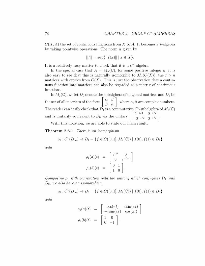
78 CHAPTER 2. GROUP C∗-ALGEBRAS
C(X,A) the set of continuous functions from X to A. It becomes a ∗-algebraby taking pointwise operations. The norm is given by
‖f‖ = sup{‖f(x)‖ | x ∈ X}.
It is a relatively easy matter to check that it is a C∗-algebra.In the special case that A = Mn(C), for some positive integer n, it is
also easy to see that this is naturally isomorphic to Mn(C(X)), the n × nmatrices with entries from C(X). This is just the observation that a contin-uous function into matrices can also be regarded as a matrix of continuousfunctions.
In M2(C), we let D0 denote the subalgbera of diagonal matrices and D1 be
the set of all matrices of the form
[α ββ α
], where α, β are complex numbers.
The reader can easily check thatD1 is a commutative C∗-subalgebra ofM2(C)
and is unitarily equivalent to D0 via the unitary
[2−1/2 2−1/2
−2−1/2 2−1/2
].
With this notation, we are able to state our main result.
Theorem 2.6.1. There is an isomorphism
ρ1 : C∗(D∞)→ B1 = {f ∈ C([0, 1],M2(C)) | f(0), f(1) ∈ D1}
with
ρ1(a)(t) =
[eiπt 00 e−iπt
]ρ1(b)(t) =
[0 11 0
].
Composing ρ1 with conjugation with the unitary which conjugates D1 withD0, we also have an isomorphism
ρ0 : C∗(D∞)→ B0 = {f ∈ C([0, 1],M2(C)) | f(0), f(1) ∈ D0}
with
ρ0(a)(t) =
[cos(πt) i sin(πt)−i sin(πt) cos(πt)
]ρ0(b)(t) =
[1 00 −1
].
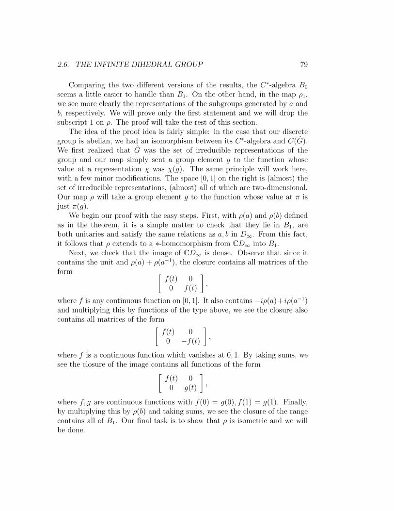
2.6. THE INFINITE DIHEDRAL GROUP 79
Comparing the two different versions of the results, the C∗-algebra B0
seems a little easier to handle than B1. On the other hand, in the map ρ1,we see more clearly the representations of the subgroups generated by a andb, respectively. We will prove only the first statement and we will drop thesubscript 1 on ρ. The proof will take the rest of this section.
The idea of the proof idea is fairly simple: in the case that our discretegroup is abelian, we had an isomorphism between its C∗-algebra and C(G).We first realized that G was the set of irreducible representations of thegroup and our map simply sent a group element g to the function whosevalue at a representation χ was χ(g). The same principle will work here,with a few minor modifications. The space [0, 1] on the right is (almost) theset of irreducible representations, (almost) all of which are two-dimensional.Our map ρ will take a group element g to the function whose value at π isjust π(g).
We begin our proof with the easy steps. First, with ρ(a) and ρ(b) definedas in the theorem, it is a simple matter to check that they lie in B1, areboth unitaries and satisfy the same relations as a, b in D∞. From this fact,it follows that ρ extends to a ∗-homomorphism from CD∞ into B1.
Next, we check that the image of CD∞ is dense. Observe that since itcontains the unit and ρ(a) + ρ(a−1), the closure contains all matrices of theform [
f(t) 00 f(t)
],
where f is any continuous function on [0, 1]. It also contains −iρ(a)+iρ(a−1)and multiplying this by functions of the type above, we see the closure alsocontains all matrices of the form[
f(t) 00 −f(t)
],
where f is a continuous function which vanishes at 0, 1. By taking sums, wesee the closure of the image contains all functions of the form[
f(t) 00 g(t)
],
where f, g are continuous functions with f(0) = g(0), f(1) = g(1). Finally,by multiplying this by ρ(b) and taking sums, we see the closure of the rangecontains all of B1. Our final task is to show that ρ is isometric and we willbe done.
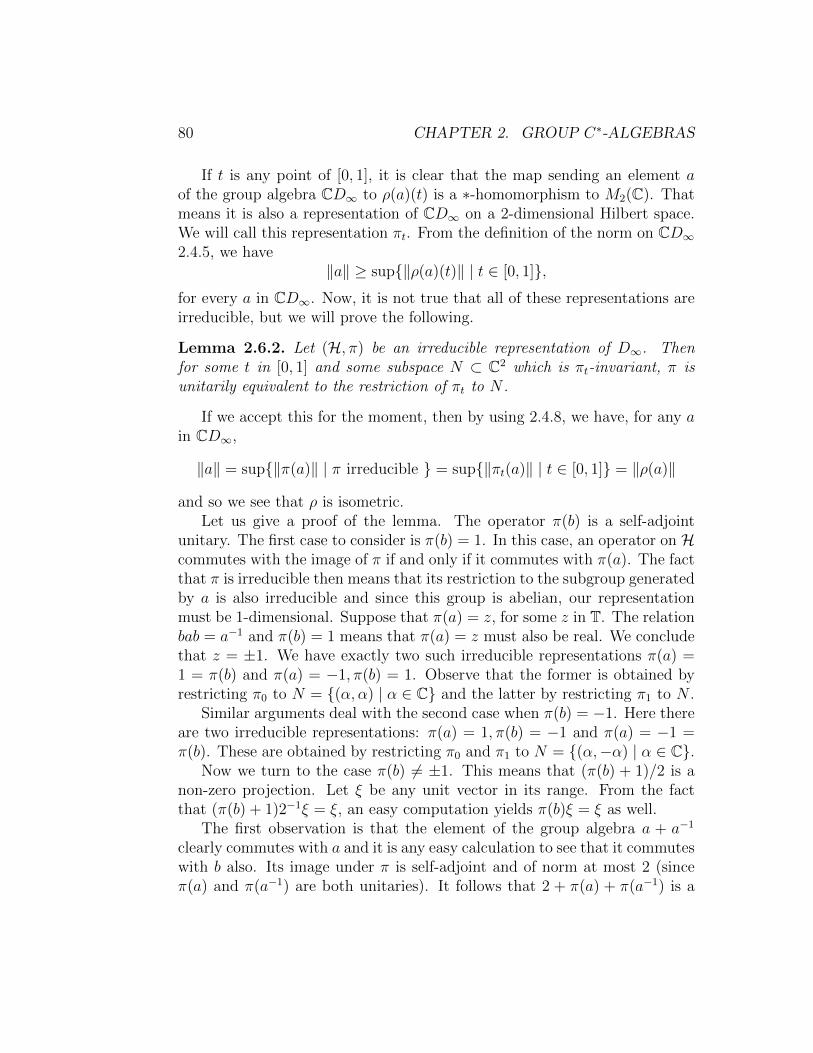
80 CHAPTER 2. GROUP C∗-ALGEBRAS
If t is any point of [0, 1], it is clear that the map sending an element aof the group algebra CD∞ to ρ(a)(t) is a ∗-homomorphism to M2(C). Thatmeans it is also a representation of CD∞ on a 2-dimensional Hilbert space.We will call this representation πt. From the definition of the norm on CD∞2.4.5, we have
‖a‖ ≥ sup{‖ρ(a)(t)‖ | t ∈ [0, 1]},for every a in CD∞. Now, it is not true that all of these representations areirreducible, but we will prove the following.
Lemma 2.6.2. Let (H, π) be an irreducible representation of D∞. Thenfor some t in [0, 1] and some subspace N ⊂ C2 which is πt-invariant, π isunitarily equivalent to the restriction of πt to N .
If we accept this for the moment, then by using 2.4.8, we have, for any ain CD∞,
‖a‖ = sup{‖π(a)‖ | π irreducible } = sup{‖πt(a)‖ | t ∈ [0, 1]} = ‖ρ(a)‖
and so we see that ρ is isometric.Let us give a proof of the lemma. The operator π(b) is a self-adjoint
unitary. The first case to consider is π(b) = 1. In this case, an operator on Hcommutes with the image of π if and only if it commutes with π(a). The factthat π is irreducible then means that its restriction to the subgroup generatedby a is also irreducible and since this group is abelian, our representationmust be 1-dimensional. Suppose that π(a) = z, for some z in T. The relationbab = a−1 and π(b) = 1 means that π(a) = z must also be real. We concludethat z = ±1. We have exactly two such irreducible representations π(a) =1 = π(b) and π(a) = −1, π(b) = 1. Observe that the former is obtained byrestricting π0 to N = {(α, α) | α ∈ C} and the latter by restricting π1 to N .
Similar arguments deal with the second case when π(b) = −1. Here thereare two irreducible representations: π(a) = 1, π(b) = −1 and π(a) = −1 =π(b). These are obtained by restricting π0 and π1 to N = {(α,−α) | α ∈ C}.
Now we turn to the case π(b) 6= ±1. This means that (π(b) + 1)/2 is anon-zero projection. Let ξ be any unit vector in its range. From the factthat (π(b) + 1)2−1ξ = ξ, an easy computation yields π(b)ξ = ξ as well.
The first observation is that the element of the group algebra a + a−1
clearly commutes with a and it is any easy calculation to see that it commuteswith b also. Its image under π is self-adjoint and of norm at most 2 (sinceπ(a) and π(a−1) are both unitaries). It follows that 2 + π(a) + π(a−1) is a
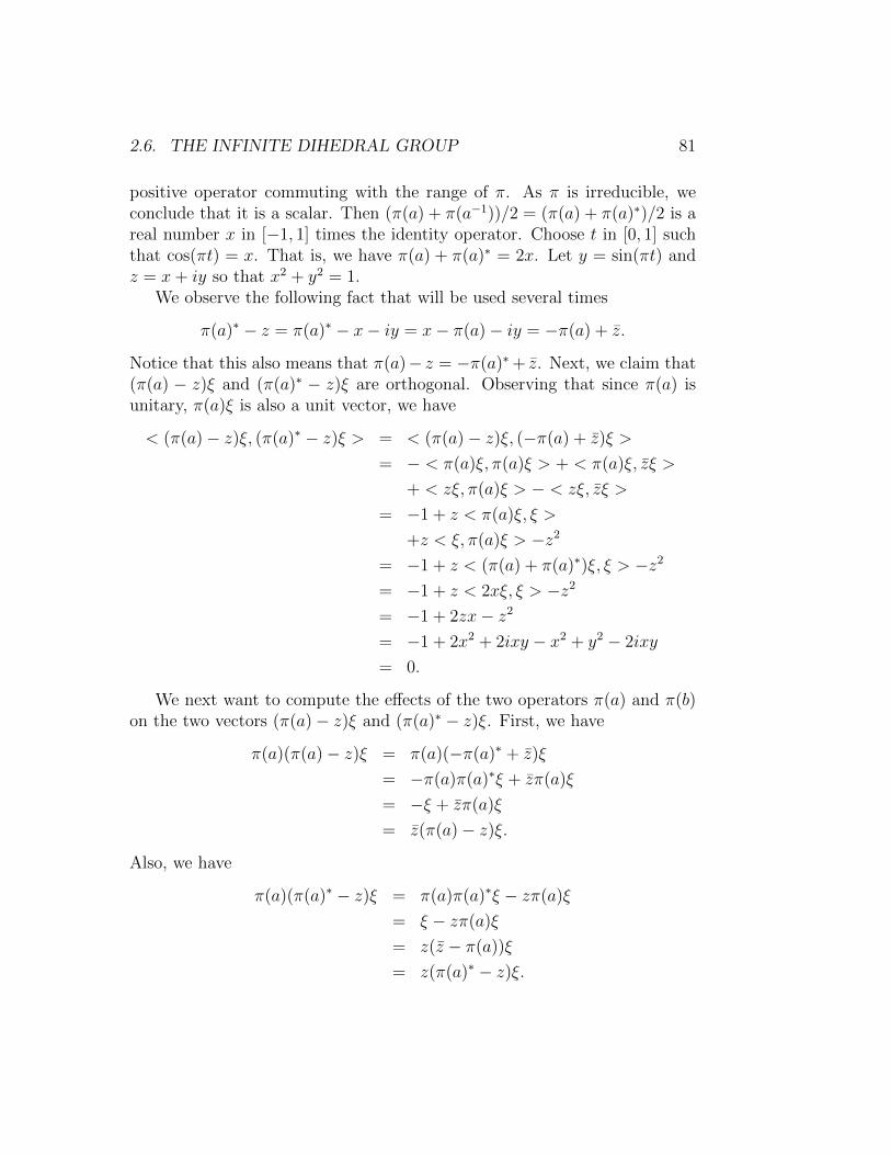
2.6. THE INFINITE DIHEDRAL GROUP 81
positive operator commuting with the range of π. As π is irreducible, weconclude that it is a scalar. Then (π(a) + π(a−1))/2 = (π(a) + π(a)∗)/2 is areal number x in [−1, 1] times the identity operator. Choose t in [0, 1] suchthat cos(πt) = x. That is, we have π(a) + π(a)∗ = 2x. Let y = sin(πt) andz = x+ iy so that x2 + y2 = 1.
We observe the following fact that will be used several times
π(a)∗ − z = π(a)∗ − x− iy = x− π(a)− iy = −π(a) + z.
Notice that this also means that π(a)− z = −π(a)∗+ z. Next, we claim that(π(a) − z)ξ and (π(a)∗ − z)ξ are orthogonal. Observing that since π(a) isunitary, π(a)ξ is also a unit vector, we have
< (π(a)− z)ξ, (π(a)∗ − z)ξ > = < (π(a)− z)ξ, (−π(a) + z)ξ >
= − < π(a)ξ, π(a)ξ > + < π(a)ξ, zξ >
+ < zξ, π(a)ξ > − < zξ, zξ >
= −1 + z < π(a)ξ, ξ >
+z < ξ, π(a)ξ > −z2
= −1 + z < (π(a) + π(a)∗)ξ, ξ > −z2
= −1 + z < 2xξ, ξ > −z2
= −1 + 2zx− z2
= −1 + 2x2 + 2ixy − x2 + y2 − 2ixy
= 0.
We next want to compute the effects of the two operators π(a) and π(b)on the two vectors (π(a)− z)ξ and (π(a)∗ − z)ξ. First, we have
π(a)(π(a)− z)ξ = π(a)(−π(a)∗ + z)ξ
= −π(a)π(a)∗ξ + zπ(a)ξ
= −ξ + zπ(a)ξ
= z(π(a)− z)ξ.
Also, we have
π(a)(π(a)∗ − z)ξ = π(a)π(a)∗ξ − zπ(a)ξ
= ξ − zπ(a)ξ
= z(z − π(a))ξ
= z(π(a)∗ − z)ξ.
82 CHAPTER 2. GROUP C∗-ALGEBRAS
Now we turn to the action of π(b) (which is simpler):
π(b)(π(a)− z)ξ = (π(b)π(a)− zπ(b))ξ
= (π(a)∗π(b)− zπ(b))ξ
= (π(a)∗ − z)π(b)ξ
= (π(a)∗ − z)ξ.
A similar computation shows that π(b)(π(a)∗ − z)ξ = (π(a)− z)ξ.It is clear from these equations that the subspace spanned by these two
vectors is invariant under π. Since the unitary π(b) maps one to the other,they must have the same length. If that happens to be zero, then π(a)ξ = zξand π(a)∗ξ = zξ. It follows that z = ±1 and that the span of ξ itself isinvariant under π. It is a simple matter to check that we have listed allthe 1-dimensional respresentation above and accounted for them with π0 andπ1 already. Otherwise, we may re-scale these vectors so that they are unitlength and, with respect to that basis, π is the same as πt. This completesthe proof of Theorem 2.6.1.
Leaving all these calculations aside, what have we learned from this ex-ample? The set of all irreducible representations of a discrete group G isusually denoted by G (which extends the definition we had before from theabelian case). The first thing we see is that a thorough understanding of thisset is important to understand C∗(G). Secondly, we can loosely interpretC∗(G) as C(G), even beyond the abelian case, if we allow the functions totake values in matrix algebras. Underlying all of this is the fact that G canbe equipped with a natural topology. We did this in the abelian case and wewon’t discuss the general, but notice here that the space is non-Hausdorff:it’s an open interval with two limit points at each end.
Finally, we remark that the short version of what we have done is to realizethat our group D∞ is composed of two abelian subgroups, Z and Z2. In short,we are able to get complete information about the irreducible representationsof D∞ from the same information about the two constituents. This is calledthe Mackey machine after George Mackey, one of the leading figures in thetheory of group representations. In brief, if one has a normal subgroup H ina group G, there is a natural construction of irreducible representations of Gfrom those of H. More impressively, this will often be exhaustive.
Exercise 2.6.1. For n ≥ 3, let Dn be the dihedral group of order 2n. Thatis,
Dn = {e, a, a2, . . . , an−1, b, ab, a2b, . . . , an−1b},
2.7. THE GROUP F2 83
where a, b satisfy an = e, b2 = e, bab = a−1.
1. List all the irreducible representations of Dn. (Hint: each of these alsogives an irreducible representation of D∞.)
2. Describe C∗(Dn).
2.7 The group F2
In this section, we investigate the C∗-algebras associated with the free groupon two generators, denoted F2. Here, the key point is that C∗-algebra isplural: the full and reduced C∗-algebras are different. This is because F2 isnot amenable. Rather than go too far into that, we will mainly concentrateon just how different these C∗-algebras are.
We will begin with a brief review of the group F2. We denote the gen-erators by a and b. A word in a, b, a−1, b−1 is simply a finite string of thesesymbols written sequentially. There is also a special word e which is theempty word consisting of no symbols. Two words may be concatenated bysimply writing them side by side. Of course, the order matters. We denotethe concatenation of w1 and w2 by w1w2. Notice that ew = w = we for all wand that concatenation is an associative operation. We define an equivalencerelation on the set of all words by first setting
w1w2 ∼ w1a−1aw2 ∼ w1aa
−1w2 ∼ w1b−1bw2 ∼ w1bb
−1w2,
for all words w1, w2 and then letting ∼ denote the transitive closure of thisrelation. We also say that a word is reduced if it contains no pair a, a−1 orb, b−1 adjacent. Each ∼-equivalence class contains a unique reduced word.The collection of ∼-equivalence classes of words, with concatenation is ourgroup F2.
The main feature of the group (in fact, it is really the definition) is that,given any group G with two elements g, h in G, there is a unique grouphomomorphism α : F2 → G such that α(a) = g and α(b) = h.
As we said above, our aim is to show that the C∗-algebras C∗(F2) andC∗r (F2) are very different. Compare them with the following two theorems.
Theorem 2.7.1. If A is a unital C∗-algebra containing unitaries u, v, thenthere exists a unique unital ∗-homomorphism ρ : C∗(F2) → A such thatρ(a) = u, ρ(b) = v. In particular, for every n ≥ 1, there is a surjective∗-homomorphism ρ : C∗(F2)→Mn(C).
84 CHAPTER 2. GROUP C∗-ALGEBRAS
Theorem 2.7.2. The C∗-algebra C∗r (F2) is simple; that is, it has no non-trivial ideals. In particular, it has no finite-dimensional representations.
Theorem 2.7.3. The trace on C∗r (F2) is unique.
Let us start by proving Theorem 2.7.1. Choose π : A → B(H) which isa faithful, unital representation. Then π(u) and π(v) are unitaries. Thatmeans there is a group homomorphism α : F2 → U(H) which maps a toπ(u) and b to π(v). This means that α is a unitary representation of F2 andextends to β, a unital representation of CF2 and also a unital representationof C∗(F2). It is clear that the image of the former is contained in the ∗-algebra generated by π(u) and π(v) while the image of the latter is in theclosure of this. In any case, both images are contained in π(A). We are donewhen we let ρ = π−1 ◦ β.
For the second statement, it is a fairly simple matter to see that thesmallest C∗-algebra which contains
u =
1 0 · · · 00 e2πi/n · · · 0...
...0 0 · · · e2πi(n−1)/n
is the set of diagonal matrices. It follows that the smallest C∗-algebra whichcontains this and
v =
0 1 0 · · · 00 0 1 · · · 0...
...0 0 11 0 · · · 0
is Mn(C).
Now we turn to the reduced C∗-algebra, which is trickier. We start witha fairly useful result that the trace is faithful.
Theorem 2.7.4. Let G be a discrete group. If c is in C∗r (G) and τ(c∗c) = 0,then c = 0. That is, the trace on C∗r (G) is faithful.
Proof. In this proof, we identify C∗r (G) with its image under πλ. Let g be in
2.7. THE GROUP F2 85
G and compute
‖cδg‖2 = < cδg, cδg >
= < cλgδe, cλgδe >
= < λ∗gc∗cλgδe, δe >
= τ(λ∗gc∗cλg)
= τ(λgλ∗gc∗c)
= τ(c∗c)
= 0.
We see that c is zero on a basis for `2(G) and hence is zero.
We next turn to some much more technical results. The next is partic-ularly opaque. Of course, we will find it useful. To put the result in somekind of informal way, the expression within the norm on left hand side ofthe conclusion is a kind of averaging process being applied to the operatorc. The result shows that this substantially reduces the norm, under certainhypotheses. The reader might want to try Exercise 2.7.4 as a little warm-upin a different setting.
Lemma 2.7.5. Let H0,H1 be Hilbert spaces. Suppose that c is an operator
on H0 ⊕ H1 having the form
[0 0∗ ∗
],
[0 ∗0 ∗
]or
[0 ∗∗ ∗
]. Also suppose
that u1, . . . , uN are unitaries such that u∗mun has the form
[∗ ∗∗ 0
], for all
m 6= n. Then we have
‖ 1
N
N∑n=1
uncu∗n‖ ≤
2√N‖c‖.
Proof. We first consider the case c =
[0 0∗ ∗
]. If d =
[∗ ∗0 0
], then we
have c∗d = d∗c = 0 so
‖c+ d‖2 = ‖(c+ d)∗(c+ d)‖ = ‖c∗c+ d∗d‖ ≤ ‖c∗c‖+ ‖d∗d‖ = ‖c‖2 + ‖d‖2.
Next, it is easy to see that for all n > 1, we have
dn = (u∗1un)c(u∗1un)∗ =
[∗ ∗∗ 0
] [0 0∗ ∗
] [∗ ∗∗ 0
]=
[∗ ∗0 0
].
86 CHAPTER 2. GROUP C∗-ALGEBRAS
Summing over n > 1 yields a term of the same form. Combining these twotogether, we have
‖N∑n=1
uncu∗n‖2 = ‖u1(c+
N∑n=2
u∗1unc(u∗1un)∗)u∗1‖2
= ‖c+N∑n=2
u∗1unc(u∗1un)∗‖2.
Now we are in a position to apply our computation above with d being thesum on the right. This yields
‖N∑n=1
uncu∗n‖2 ≤ ‖c‖2 + ‖
N∑n=2
u∗1unc(u∗1un)∗‖2
= ‖c‖2 + ‖N∑n=2
uncu∗n‖2.
Continuing by induction, dividing by N2 and taking square roots yields theanswer, without the factor of 2.
The second case for c is obtained simply by taking adjoints of the first.For the third, any such c can be written as p0c+p1c, where pi is the orthogonalprojection of H0 ⊕H1 onto Hi, i = 0, 1. We can apply the first and secondcases to p0c and p1c respectively to get
‖ 1
N
N∑n=1
uncu∗n‖ ≤
1√N‖p0c‖2 +
1√N‖p1c‖2 ≤ 2√
N‖c‖2.
We are going to apply this to the elements of the left regular representa-tion of F2.
Lemma 2.7.6. For all w in F2, we have
limN→∞
1
N
N∑n=1
λanλwλa−n =
{λw w = ak, k ∈ Z0 otherwise
2.7. THE GROUP F2 87
Proof. First of all, if w is a power of a, then for each n, λanλwλa−n = λw andthe conclusion is clear. If not, then w contains either a b or b−1. Then wehave w = akw0a
l, where w0 begins and ends in b or b−1 (including the casethat it is a power of b).
Let H0 be the span of all δw′ where w′ is empty or begins with a±1. Alsolet H1 be the span of the remaining elements of the group, those which beginwith b±1.
We make two simple observations: λw0H0 ⊂ H1 and λaH1 ⊂ H0. Itfollows that b = λw0 and ui = λai , 1 ≤ i ≤ n satisfy the hypotheses ofLemma 2.7.5. Hence, we have
limN‖ 1
N
N∑n=1
λanλwλa−n‖ = limN‖ 1
N
N∑n=1
λanλakλw0λalλa−n‖
= limN‖ 1
N
N∑n=1
λanλw0λa−n‖
≤ limN
1√N‖λw0‖
= 0.
Lemma 2.7.7. For any c in C∗r (F2), we have
limM,N→∞
1
MN
M∑m=1
N∑n=1
λbnamcλa−mb−n = τ(c).
Proof. By some standard estimates, it suffices to check this on elements ofthe group algebra CF2. Then by linearity, it suffices to check it for c = λw,for some w in F2.
The first case to consider is when w is the identity element and then theconclusion is clear. The second is that w = ak, for some k 6= 0. In this case,λw commutes with each λan and so we get
limM,N→∞
1
MN
M∑m=1
N∑n=1
λbnamcλa−mb−n = limN→∞
1
N
N∑n=1
λbncλb−n
and the conclusion is an application of the last Lemma (with b replacing a).
88 CHAPTER 2. GROUP C∗-ALGEBRAS
The final case is for w 6= ak, for any integer k. Then given ε > 0, we mayfind N0 such that for all N ≥ N0, we have
‖ 1
N
N∑n=1
λanλwλa−n‖ < ε.
Then for every m, we also have
‖ 1
N
N∑n=1
λbmanλwλa−nb−m‖ < ε.
and hence
‖ 1
MN
M∑m=1
N∑n=1
λbnamcλa−mb−n‖ < ε,
provided N ≥ N0. This completes the proof.
We are now ready to prove Theorem 2.7.2. Suppose that C∗r (F2) has anon-zero ideal I and let c be some non-zero element of that ideal. We knowfrom Theorem 2.7.4 that τ(c∗c) > 0. We also know that c∗c is also in theideal. Looking at the last Lemma, the expression on the left hand side (usingc∗c instead of c) lies in the ideal, for every value of M,N . As the ideal isclosed, τ(c∗c) > 0 is in the ideal. But this element is invertible and it followsthat I = C∗r (F2).
As for the proof of Theorem 2.7.3, if φ is any other trace on C∗r (F2), ifwe apply it to 1
MN
∑Mm=1
∑Nn=1 λbnamcλa−mb−n we clearly get φ(c) because of
the trace property. On the other hand, applying it to the scalar τ(c) yieldsτ(c). The conclusion follows from Lemma 2.7.7.
Exercise 2.7.1. Let u be the N ×N unitary matrix
u =
1 0 · · · 00 e2πi/N · · · 0...
...0 0 · · · e2πi(N−1)/N
.Define a map E : MN(C)→MN(C) by
E(a) =1
N
N∑n=1
unau−n,
for a in MN(C).
2.8. LOCALLY COMPACT GROUPS 89
1. Prove that the range of E is contained in the C∗-subalgebra D consistingof diagonal matrices.
2. Prove that E(d) = d if d is diagonal. In consequence, E ◦ E = E.
3. Prove that E(a∗a) is positive for every a in MN(C).
4. Prove that E is faithful, meaning that if E(a∗a) = 0, for some a inMN(C), then a = 0.
5. Prove that if a in MN(C) and c, d are in D, then E(cad) = cE(a)d.
6. Prove that ‖E‖ = 1.
Exercise 2.7.2. Let u, v be the N ×N unitary matrices
u =
1 0 · · · 00 e2πi/N · · · 0...
...0 0 · · · e2πi(N−1)/N
, v =
0 1 0 · · · 00 0 1 · · · 0...
...0 0 11 0 · · · 0
.
Prove that, for any c in MN(C), we have
1
N2
N∑m=1
N∑n=1
vnumcu−mv−n = τ(c),
where τ is the usual trace on MN(C).
Exercise 2.7.3. Show that Theorem 2.7.3 is false for C∗(G).
2.8 Locally compact groups
In this section, we discuss, informally, a more general construction of thegroup C∗-algebra. The starting point is the notion of a topological group.By a topological group we mean a group G, endowed with a topology in whichthe product, regarded as a map from G×G (with the product topology) toG, and the inverse, regarded as a map from G to itself, are both continuous.It is frequently assumed that G is Hausdorff.
90 CHAPTER 2. GROUP C∗-ALGEBRAS
There are many examples. Of course, any group at all, given the discretetopology will qualify. The real numbers with the usual operation of additionand the usual topology is also an example. So is the circle group T. A moreexotic example is GL(n,R), the set of invertible real n × n matrices withmatrix multiplication as group operation.
The first fundamental new ingredient is a left-invariant measure calledthe Haar measure.
Theorem 2.8.1. Let G be a locally compact, Hausdorff group. There exists apositive regular Borel measure µ on G with the property that µ(gE) = µ(E),for all Borel sets E ⊂ G and g ∈ G, where gE = {gh | h ∈ E}. Moreoverthis measure is unique, up to a scalar multiple.
In the case that the group G is discrete, Haar measure is simply countingmeasure.
A complete treatment of this subject would start with a proof of thiscrucial fact, which is why we aren’t going to do that.
Let us take a little detour for a moment to return to the topic of discreteabelian groups which was covered in section 2.5. Recall that we had anisomorphism from C∗(G) to C(G); let us denote it by α for the moment. Weobserved earlier that G is both a group and a compact, Hausdorff topologicalspace. It is a fairly easy thing to see that it is actually a topological group.Hence, it has a Haar measure, µ. This measure is actually finite in this case,so we assume µ(G) = 1. With this measure available, we have a very nicedescription of the inverse of our isomorphism. Suppose that f is in C(G).Then we have
α−1(f)(g) =
(∫f(χ)χ(g)dµ(χ)
)This should be recognizable. When G = Z and G = T, the right hand sideis the conventional Fourier series for f . Notice that we are defining α−1(f)as a function on G. In fact, we have to be very careful with this and exactlywhich f we use. Some care is needed when discussing the map above; thesame formula also defines a unitary operator between L2(G, µ) and `2(G).
We now return to the general case of topological groups which are notnecessarily abelian. There is an interesting and useful consequence of theuniqueness of the Haar measure as follows. If we fix a group element g in G,and look at the function defined on Borel sets E by µg(E) = µ(Eg), it is clearthat this is also a left-invariant measure. Hence there is a constant ∆(g) such
2.8. LOCALLY COMPACT GROUPS 91
that µg = ∆(g)µ. The function ∆ : G→ R+ is a group homomorphism (withrange having multiplication as group operation). The function is identicallyone if and only if the left-invariant measure happens to be right-invariant aswell.
Our first step, when we had a discrete group, was to form the groupalgebra. Of course, one can still do this, but instead we will consider Cc(G),the continuous complex-valued functions of compact support on G, ratherthan CG which are the functions of finite support. If G is discrete, this isjust CG as before. Notice here that the inclusion G ⊂ Cc(G) fails unless Gis discrete, since a function that is one at a single group element and zeroelsewhere will not be continuous if the group is not discrete.
We regard Cc(G) as a linear space in the obvious way and define theproduct by the formula
ab(g) =
∫h∈G
a(h)b(h−1g)dµ(h),
for all a, b in Cc(G) and g in G. We also define an involution by
a∗(g) = ∆(g)−1a(g−1),
for all a in Cc(G) and g in G.We leave it for the reader to verify that Cc(G) is a ∗-algebra with this
product and involution. The computations are not a complete triviality sinceone sees rather concretely exactly why the measure needs to be left-invariantand also why the function ∆ makes its surprise entrance in the involution. Ofcourse, if G is discrete, the measure is simply counting measure, the integralsimply becomes a sum and our product is exactly the same as we saw inTheorem 2.4.2. In addition, counting measure is clearly right-invariant aswell as left-invariant and this is why ∆ did not appear earlier in the Chapter.
The other important thing to notice here is that Cc(G) has no unit unlessG is discrete. Essentially, this is the same issue that Cc(G) does not containG.
We also define a norm on Cc(G) by the formula
‖a‖1 =
∫g∈G|a(g)|dµ(g),
for all a in Cc(G). The completion of Cc(G) in this norm is L1(G). Exceptfor the change of ` to L, this is the same as the discrete case. In fact, the
92 CHAPTER 2. GROUP C∗-ALGEBRAS
formulae we have above also hold for the product and involution on L1(G)making it a Banach algebra with an isometric involution.
The next item that requires modification is the notion of unitary represen-tation. Usually in the case of a topological group G, a unitary representationis (u,H), where H is a Hilbert space as before, u is a group homomorphismfrom G to the unitary group on H and we require that u is continuous whenG is considered with its given topology and the unitaries are considered withthe strong operator topology. The left regular representation is defined ex-actly as before, replacing `2(G) by L2(G, µ), where µ is Haar measure. Thefact that the operators λg, g ∈ G, are unitary is a direct consequence of thefact that the Haar measure is left-invariant. It should also be checked thatthis is continuous in the sense above.
Why is this the right thing to do? The crucial result which persistsfrom the discrete case here is that there are bijective correspondences be-tween: unitary representations of G, non-degenerate representations of Cc(G)(though not unital since Cc(G) has no unit in general) and non-degeneraterepresentations of L1(G). The passage from first to second to third is verymuch as before. If (u,H) is a unitary representation of G, then, for any a inCc(G), the formula
πu(a) =
∫g∈G
a(g)ug
defines a bounded linear operator. Also, this formula will extend continu-ously to define πu on L1(G). It is in going back that subtleties arise. Ofcourse, Cc(G) ⊂ L1(G) is valid, but one cannot restrict to G ⊂ Cc(G) toget from representations of the ∗-algebras back to unitary representations ofthe group. Nevertheless, the definitions of the full and reduced norms andthe completions of the group algebras into C∗-algebras C∗(G) and C∗r (G)proceeds as before.
In the special case that G is commutative, but not necessarily discrete,we again know that C∗(G) will be isomorphic to C0(X), for some locallycompact space X. In fact, the space X is again the dual group:
G = {χ : G→ T | χ a continuous group homomorphism }.
The only new item here is the word ’continuous’ (which can obviously beomitted with no change if the group happens to be discrete). Again, we havethe isomorphism C∗(G) ∼= C0(G). It is interesting to note that we can stilldefine, for any group element g, the function g(χ) = χ(g), χ ∈ G. The only
2.8. LOCALLY COMPACT GROUPS 93
problem now with the map g → g is that g is not an element of Cc(G), noris g in C0(G), when G is not discrete.
Of course, we have been assuming implicitly here that G has a topology.Let us just spell out exactly what that is, particularly since it will be nice tosee the parallel with the discrete case before. For each χ in G, K ⊂ G whichis compact and ε > 0, we define
U(K, ε) = {χ′ ∈ G | |χ′(g)− χ(g)| < ε, for all g ∈ K}.
These sets form a neighbourhood base for a topology on G. In this topology,G is again a topological group.
As an example, we have R ∼= R and the isomorphism, which we findconvenient to write here as a pairing, is given by
< r, s >= e2πirs, r, s ∈ R.
That is, if one fixes s, this defines a map χs(r) =< r, s > from R to thecircle which is a continuous group homomorphism. Moreover, s → χs is anisomorphism between R and R.
It is again true here that the inverse of the isomorphism α from C∗(G)to C0(G) is given by Fourier transform
α−1(f)(r) =
∫Rf(s)e−2πirsds,
for f in Cc(R) and r in R, or for a general abelian topological group G,
α−1(f)(g) =
∫G
f(χ)< g, χ >dµ(χ),
for f in Cc(G) and g in G.
Exercise 2.8.1. Let G be a locally compact Hausdorff group. Prove that ifHaar measure is counting measure, then G is discrete.
Exercise 2.8.2. Let G be the ax+ b group:
G =
{[a b0 1
]| a > 0, b ∈ R
}with matrix multiplication as group operation. (There is a little ambiguityhere: sometimes one takes a 6= 0 instead.)
94 CHAPTER 2. GROUP C∗-ALGEBRAS
1. Prove that a−2dadb is the Haar measure on G. (That is, it is Lebesguemeasure on (0,∞)×R times the function (a, b)→ a−2.) In other words,if we let E be the set of all matrices with a in [a1, a2] and b in [b1, b2],then
µ(E) = (a−11 − a−1
2 )(b2 − b1).
2. Find ∆.
Chapter 3
Groupoid C∗-algebras
We have so far seen two very important constructions of C∗-algebras. To anylocally compact Hausdorff space X, we have C0(X). In fact, this constructionyields exactly the class of commutative C∗-algebras. The other constructionassociates a C∗-algebra C∗(G) to any discrete group G. In fact, there is alsoC∗r (G) as well, so this particular construction yields (potentially) two (ormore) C∗-algebras.
Our next objective is a construction which combines these two, in somesense. In particular, these will both be seen as special cases of our new con-struction. That sounds impressive, but we should warn readers that, ratherthan expecting some elegant general structure which subsumes both, what weconstruct, etale groupoids, really look a little more like some Frankenstein-type monster, built out of parts of both.
The goal though is not so unreasonable and let us take a few minutes toexplain why, at least for people with some interest in topological dynamicalsystems. (Ergodic theorists will probably already have realized that theyshould be looking in the direction of von Neumann algebras.)
What is a topological dynamical system? A reasonable simple answeris that is a continuous self-map, ϕ, of topological space, X. But that ismisleading, even if it is not deliberately so. It would be impossible to doany mathematics that one could legitimately call dynamical systems withoutiterating the map. From this point of view, the dynamical system reallyconsists of a collections of maps, ϕn, n ≥ 1, with the condition that ϕn◦ϕm =ϕn+m, for all n,m ≥ 1. Here, one sees at once that the collection of mapscontains some algebraic structure. In this case, it is that of the semigroupof natural numbers. Of course, in any general theory, groups are simpler
95
96 CHAPTER 3. GROUPOID C∗-ALGEBRAS
than semigroups and so we would prefer to assume that ϕ is actually ahomeomorphism and consider the family of maps indexed by Z rather thanN. Even in this simple case, we can see that we would like to consider asingle C∗-algebra which is built from C0(X) and C∗(Z). Of course, the twoof these separately aren’t very much use since neither remembers on its ownwhat ϕ is.
3.1 Groupoids
We begin with the definition of a groupoid. As the name would suggest,it is rather like that of a group. The key point is that the product of anarbitrary pair of elements may not be defined. That is, we specify a subset(called G2) of G × G and the product gh is only defined for pairs (g, h)in G2. The first axiom is a fairly natural generalization of associativity.One might reasonably expect the next axiom to concern the existence of anidentity. That is actually too much to ask. Instead, the other axiom is thatthere is an inverse operation g → g−1. The condition is rather subtle, butwhat it contains is that g−1g and gg−1 will serve as an identities for certainelements. In particular, the former is a right identity for g and the latter is aleft identity. These may not be equal; indeed G may have a large collectionof identities.
Definition 3.1.1. A groupoid is a non-empty set G, together with a subsetG2 ⊂ G × G, a map from G2 to G (the image of (g, h) is denoted gh) andan involution, g → g−1, satisfying the following conditions.
1. If g, h, k are in G with (g, h), (h, k) both in G2, then so are (gh, k) and(g, hk) and we have (gh)k = g(hk). (We write the result as ghk.)
2. For all g in G, both (g, g−1) and (g−1, g) are in G2. If (g, h) is in G2,then g−1gh = h. If (h, g) is in G2, then hgg−1 = h.
The following definitions will be useful. First, since there are multipleidentity elements, we prefer to call them units. The letters r, s stand forrange and source. The usefulness of this terminology will become apparentlater.
Definition 3.1.2. Let G be a groupoid. The set of units of G (or identities)is
G0 = {g−1g | g ∈ G}.
3.1. GROUPOIDS 97
We define r, s : G→ G0 by r(g) = gg−1, s(g) = g−1g.
Lemma 3.1.3. Let G be a groupoid.
1. For any g in G, (r(g), g), (g, s(g)) are in G2 and r(g)g = gs(g) = g.
2. If g, h are elements of G, then (g, h) is in G2 if and only if s(g) = r(h).
3. If g, h are elements of G with (g, h) in G2, then (h−1, g−1) is in G2 and(gh)−1 = h−1g−1.
4. If g, h are elements of G with (g, h) in G2, then r(gh) = r(g) ands(gh) = s(h).
5. If g is in G0, then g−1 = g.
6. If g is in G0, then r(g) = s(g) = g.
Proof. The first statement is just a re-writing of the previous definition inthe special case g = h.
For the second part, if (g, h) is in G2, we know that (g−1, g), (h, h−1) arealso and
s(g) = g−1g = g−1(ghh−1) = (g−1gh)h−1 = hh−1 = r(h).
Conversely, suppose that s(g) = r(h). We know that (g, g−1) and (g−1, g)are in G2, so (g, g−1g) is in G2. Since g−1g = s(g) = r(h) = hh−1, we have(g, hh−1) is in G2. Similar arguments show that (hh−1, h) is in G2 and hence(g, h) = (g, hh−1h) is in G2 as desired.
For the third part, from associativity, we know that (gh)h−1 is defined andequals g. It follows then that ((gh)h−1)g−1 is also defined and equals gg−1.On the other hand ((gh)−1, gh) is inG2 and it follows that ((gh)−1, ((gh)h−1)g−1)is also and hence ((gh)−1, gg−1) is in G2. This in turn means ((gh)−1, g) isin G2 and (gh)−1gg−1 = (gh)−1 is in G2. Hence, we have
(gh)−1 = (gh)−1gg−1 = (gh)−1((gh)h−1)g−1 = h−1g−1.
For the fourth part, we make use of the third part and compute
r(gh) = gh(gh)−1 = (gh)(h−1g−1) = (g(hh−1))g−1 = gg−1 = r(g).
The other part is done similarly.
98 CHAPTER 3. GROUPOID C∗-ALGEBRAS
The fifth part follows at once from the third and the definition of G0.For the last statement, if g is in G0, then g = h−1h and using part 4, we
haves(g) = s(h−1h) = s(h) = h−1h = g.
The other part is done similarly.
The result above gives us a nice picture to have in mind of a groupoid.Imagine that we represent the elements of G0 as vertices and each elementg in G as an edge, starting at s(g) and terminating at r(g). The product isthen a rule which assigns to each pair g, h with s(g) = r(h), a new edge ghgoing from s(h) to r(g). There is a small problem with this: is an elementof G0 a vertex or an edge or both? I find it convenient to let G \G0 be theedges. The success of this picture varies, case by case.
It is a good time to look at some examples.
Example 3.1.4. Any group G is a groupoid. Use G2 = G × G. HereG0 = {e}.
Following up on this, it can be shown that a groupoid is a group if andonly if G0 contains a single element (Exercise ??). The picture we had abovefor this groupoid is particularly unhelpful. We have a single vertex and a setof edges, which are all loops. The only thing you can tell about the groupfrom the picture is the number of elements! Of course, the problem is thatthe picture doesn’t really show the product very clearly.
Example 3.1.5. Let X be any set and R be an equivalence relation on X.Define
R2 = {((x, y), (y, z)) | (x, y), (y, z) ∈ R}.Then define the product as (x, y)(y, z) = (x, z) and the inverse as (x, y)−1 =(y, x), for all (x, y), (y, z) in R. In this way, R is a groupoid with
r(x, y) = (x, y)(x, y)−1 = (x, y)(y, x) = (x, x),
s(x, y) = (y, y),
for all (x, y) in R andR0 = {(x, x) | x ∈ X}.
We denote the set on the right by ∆X . In particular, for any set X, X ×X(called the trivial equivalence relation) and ∆X (called the co-trivial equiva-lence relation) are groupoids.
3.1. GROUPOIDS 99
In contrast to the situation for groups, our picture of an equivalencerelation is quite accurate and helpful.
Proposition 3.1.6. Let G be a groupoid. The set R = {(r(g), s(g)) ∈ G0 ×G0 | g ∈ G} is an equivalence relation on G0. Moreover, if the map α(g) =(r(g), s(g)) from G to R is injective then it is an isomorphism between thegroupoids G and R. In this case, we say that G is a principal groupoid.
Let us return to a couple more general examples. The next is quite animportant one.
Example 3.1.7. Let G be a group acting (on the right) on a set X. Thatis, for each x in X and g in G, we have xg which is in X. These are suchthat, for fixed g in G, the map x→ xg is a bijection and x(gh) = (xg)h, forall g, h in G and x in X.
Consider the set X ×G and define
(X ×G)2 = {((x, g), (y, h)) | xg = y}.
Then the product and inverse are given by (x, g)(xg, h) = (x, gh) and (x, g)−1 =(xg, g−1), respectively, for x in X, g, h in G. We note that
r(x, g) = (x, g)(x, g)−1 = (x, g)(xg, g−1) = (x, e), s(x, g) = (xg, e),
for x in X, g in G, and (X ×G)0 = X × {e}.
Example 3.1.8. Let X be a topological space. Consider the set of all paths inX; i.e. continuous functions γ : [0, 1] → X. Two paths γ, γ′ are homotopicif there is a continuous function F : [0, 1] × [0, 1] → X such that F (s, 0) =γ(s), F (s, 1) = γ′(s), for all 0 ≤ s ≤ 1 and F (0, t) = γ(0) = γ′(0), F (1, t) =γ(1) = γ′(1), for all 0 ≤ t ≤ 1. That is, one path may be continuouslydeformed to the other, while holding the endpoints fixed. Homotopy is anequivalence relation. Let [γ] denote the homotopy class of γ.
Let π(X) denote the set of all homotopy classes of paths in X. We define
π(X)2 = {([γ], [γ′]) | γ(1) = γ′(0)}.
The product is given by [γ][γ′] = [γγ′], where
(γγ′)(s) =
{γ(2s) 0 ≤ s ≤ 1/2,
γ′(2s− 1) 1/2 ≤ s ≤ 1,
where γ, γ′ are paths. The inverse is given by γ−1(s) = γ(1 − s), 0 ≤ s ≤ 1.This groupoid is called the fundamental groupoid of X.
100 CHAPTER 3. GROUPOID C∗-ALGEBRAS
Now we present a couple of simple ways of constructing new groupoidsfrom old ones. The first is fairly familiar from group theory.
Example 3.1.9. If G and H are groupoids, then so is their product G×Hin an obvious way.
The next example is very unfamiliar from group theory.
Example 3.1.10. If Gι, ι ∈ I, are groupoids, then so is their disjoint unionG = tι∈IGι as follows. We define G2 = tι∈IG2
ι and the product is thenobvious.
In fact, that’s it!
Theorem 3.1.11. Every groupoid is isomorphic to the disjoint union of acollection of products of groups and equivalence relations. More precisely, ifG is a groupoid, then
G ∼= tι∈IGι × (Xι ×Xι),
where Gι is a group and Xι is a set, for all ι.
Proof. Let R be the equivalence relation on G0 from 3.1.6. Choose I to bea set which indexes the equivalence classes of R. That is, for each ι in I,Xι ⊂ G0 is an equivalence class of R, these are pairwise disjoint for differentvalues of ι and the union over all ι in I is G0. For each value of ι, choose xιin Xι. Also, for each x in Xι, we know that (x, xι) is in R, so we may choosegx in G such that r(gx) = x and s(gx) = xι.
For each ι in I, define
Gι = {g ∈ G | r(g) = s(g) = xι}.
It is easy to see that Gι is a group with identity element xι.We define a map α : tι∈IGι × (Xι ×Xι)→ G by
α(g, (x, y)) = gxgg−1y ,
for all g in Gι, x, y in Xι and ι in I. First, let us see that α is well-defined.We know that s(gx) = xι = r(g) = s(g) = s(gy) = r(g−1
y ), and so the productis well-defined.
We also define β : G→ tι∈IGι × (Xι ×Xι) by
β(g) = (g−1r(g)ggs(g), (r(g), s(g))), g ∈ G.
It is a simple exercise to see that β is well-defined and is the inverse of α.
3.2. TOPOLOGICAL GROUPOIDS 101
Of course, this result looks like the end of the road for groupoids. In fact,we will revive them in the next section by studying topological groupoids.
Exercise 3.1.1. Suppose that G is a groupoid with a single unit. Prove thatG is a group.
Exercise 3.1.2. Prove that the groupoid X×G of Example 3.1.7 is principalif and only if the action is free (that is, the only x, g for which xg = x isg = e).
Exercise 3.1.3. Suppose that g is an element of a groupoid G. Prove thatthe right identity of g is unique. That is, if h is any element of G with (g, h)in G2 and gh = g, then h = s(g).
Exercise 3.1.4. In example 3.1.8, let γ be any path in X. Find the simplestpossible paths which represent r[γ] and s[γ]. Give a complete description ofπ(X)0.
Exercise 3.1.5. Find the spaces Xι and the groups Gι in Theorem 3.1.11for the fundamental groupoid of a space X.
3.2 Topological groupoids
To get some interest back into our groupoids after Theorem 3.1.11, we intro-duce topology into the picture.
Definition 3.2.1. A topological groupoid is a groupoid G with a topologysuch that, when G2 is given the relative topology of G × G, it is closed andthe product (as a map from G2 to G) and the inverse (as a map from G toitself) are both continuous.
Let us just note an obvious fact.
Lemma 3.2.2. If G is a topological groupoid, then the maps r and s arecontinuous. If G is Hausdorff, then G0 is closed.
Proof. The map g ∈ G → g−1 ∈ G is continuous, hence so is g ∈ G →(g, g−1) ∈ G2 ⊂ G × G. The map r is simply the composition of this mapwith the product and hence is continuous. The situation for s is similar.For the last statement, if gα is a net in G0 converging to g, then we knowfrom part 6 of Lemma 3.1.3 that gα = s(gα). Taking limits and using thecontinuity of s we see that s(g) = g and hence g is in G0.
102 CHAPTER 3. GROUPOID C∗-ALGEBRAS
Let us give a couple of examples.
Example 3.2.3. Let X be any topological space. The groupoid X ×X withthe product topology is a topological groupoid. Also, the groupoid ∆X withthe relative topology from X × X (which makes the map sending x in X to(x, x) in ∆X a homeomorphism) is a topological groupoid.
Example 3.2.4. Let X be a compact space and G be a topological group(or a discrete group, if you prefer). Assume that G acts on X continuously,meaning that the map from X × G to X of Example 3.1.7 is continuous.With the product topology and the groupoid structure of 3.1.7, X × G is atopological groupoid. We will actually prove this below in Theorem 3.2.11.
Our next task is to define special classes of topological groupoids calledr-discrete groupoids and etale groupoids. The idea in both cases is essentiallythe same (although the latter is a strictly stronger condition) and we discussit a little.
When considering the C∗-algebras C0(X), we would not have got veryfar if we only considered spaces with the discrete topology. On the otherhand, our treatment of group C∗-algebras of Chapter 2 did not suffer a greatdeal by assuming the group is discrete. What we try to impose with thesetwo new conditions is that, while the groupoid itself may be continuous, the’group-like’ part of it is discrete. This idea comes out nicely in Theorem3.2.11 where the groupoids X ×G associated with an action of the group Gon the space X satisfy both these hypotheses when the group G is discrete.
Definition 3.2.5. A topological groupoid is r-discrete if G0 is open in G.
The following result will be useful and helps to explain the terminology.
Lemma 3.2.6. Let G be an r-discrete groupoid. For every g in G0, r−1{g}and s−1{g} are discrete.
Proof. Suppose that we have a net hα converging to h, all in r−1{g}. Thenr(hα) = r(h) = g, for all α. We know that s(h−1) = r(h) and so (h−1, hα) isdefined for all α. Moreover, by the continuity of the product, the net h−1hαconverges to h−1h, which is in G0. Since G0 is open, h−1hα is in G0 for allsufficiently large α. Then we know that h−1hα = s(h−1hα) = s(hα) = h−1
α hα.Right multiplying by h−1
α and taking inverse then implies hα = h, for all suchα.
3.2. TOPOLOGICAL GROUPOIDS 103
Definition 3.2.7. A map f : X → Y between two topological spaces is alocal homeomorphism if, for ever x in X, there is an open set U containingx such that f(U) is open in Y and f |U : U → f(U) is a homeomorphism.
Notice the condition that f be open is important. Otherwise the inclusionof a point in any space would satisfy the condition.
Definition 3.2.8. A topological groupoid is etale if the maps r, s are bothlocal homeomorphisms. Any set U ⊂ G which satisfies the conditions ofDefinition 3.2.7 for the maps r, s : G→ G is called a G-set.
We note the following; its proof is easy.
Theorem 3.2.9. Let G be an etale groupoid. Any open subset of a G-set isalso a G-set. If Γ is the collection of G-sets, then Γ satisfies the following.
1. If γ is in Γ, then so is γ−1.
2. If γ1, γ2 are in Γ, then so is γ1γ2.
3. If γ1, γ2 are in Γ, then so is γ1 ∩ γ2.
Moroever, Γ is a neighbourhood base for the topology on G and Γ0 = {γ∩G0 |γ ∈ Γ} is a neighbourhood base for the topology of G0.
While the definitions of r-discrete and etale are rather different looking,let us show they are at least related.
Theorem 3.2.10. Every etale groupoid is r-discrete.
Proof. If g is in G, let U be any G-set containing g. Then r(U) is an openset containing r(g) and is contained itself in G0. In this way, we see that G0
can be covered by open sets and hence is open.
Roughly speaking, the condition of r-discrete means that r is locallyinjective at any point h. The condition that G is etale means it is also ontoan open set containing r(h).
Theorem 3.2.11. Let G be a topological group and X a topological space.Assume that G acts on X (on the right) and that the map (x, g) ∈ X ×G→xg ∈ X is continuous. Then X × G as a groupoid (3.1.7) with the producttopology is a topological groupoid. If G is discrete, then X × G is both r-discrete and etale.
104 CHAPTER 3. GROUPOID C∗-ALGEBRAS
Proof. We first show that (X×G)2 is closed. If ((xα, gα), (xαgα, hα)) is a con-vergent net, then clearly xα converges to some x in X, gα converges to someg in G and hα converges to some h in G. It follows from the continuity of theaction that xαgα converges to xg. Thus, our net converges to ((x, g), (xg, h)),which is in X ×G and the limit of the products is the product of the limits.
From the fact that the inverse map on G is continuous and the hypoth-esis on the continuity of the action, we see that (x, g) → (xg, g−1) is alsocontinuous.
Now we assume that G is discrete. We compute
r(x, g) = (x, g)(x, g)−1 = (x, g)(xg, g−1) = (x, e).
It follows that, for any g in G, the set {g} is open in G and the restrictionof r to the open set X × {g} is a homeomorphism to X × {e} = (X × G)0.The case for the map s is similar. It follows that X × G is etale and hencer-discrete as well.
We note the following useful but easy result.
Theorem 3.2.12. Let G be a topological groupoid and let H ⊂ G be a sub-groupoid. Then H is also a topological groupoid (with the relative topology).If G is r-discrete, then H is also. If H is open in G and G is etale, then His also etale.
Exercise 3.2.1. Let R = {(x, x), (−1, 1), (1,−1) | −1 ≤ x ≤ 1} which isconsidered as an equivalence relation of [−1, 1] and with the relative topologyof [−1, 1]2. First, show that R is a topological groupoid. Is it r-discrete? Isit etale?
Exercise 3.2.2. Let R = {(x, x), (x,−x) | −1 ≤ x ≤ 1} which is consideredas an equivalence relation of [−1, 1] and with the relative topology of [−1, 1]2.Is R r-discrete? Is it etale?
Exercise 3.2.3. Let G = {1,−1} be the cyclic group of order two and con-sider its action on X = [−1, 1] defined by x · i = ix, for x ∈ [−1, 1] andi = ±1. Then X ×G is etale by Theorem 3.2.11. Does this fact and Propo-sition 3.1.6 imply that the equivalence relation of Exercise 3.2.2 is etale?
Exercise 3.2.4. Consider the smallest topology on R of Exercise 3.2.2 whichincludes the relative topology of [−1, 1]2 and the set ∆[−1,1]. With this topol-ogy, is R r-discrete? Is it etale? Give two explanations of the last part: onedirect and one using the action of Exercise 3.2.3 and Theorem 3.2.12.
3.3. THE C∗-ALGEBRA OF AN ETALE GROUPOID 105
Exercise 3.2.5. Let X = [0, 1]∪ [2, 3]. Let A be a subset of [0, 1] and define
R = ∆X ∪ {(x, x+ 2), (x+ 2, x) | x ∈ A},
with the relative topology of X ×X.
1. Prove that R is r-discrete.
2. Give a necessary and sufficient condition on the set A for R to be etale.
3.3 The C∗-algebra of an etale groupoid
This section is devoted to the construction of the C∗-algebra of an etalegroupoid. For convenience, and so that it parallels with the construction ofthe C∗-algebra of a discrete group, we have divided this into a sequence ofsubsections.
3.3.1 The fundamental lemma
Lemma 3.3.1. Let G be an etale groupoid. Let p denote the product mapfrom G2 to G. If U and V are G-sets, then p(U × V ∩ G2) is open in G2
and the restriction of p to U × V ∩ G2 is a homeomorphism to its image.Moreover, p(U × V ∩G2) is a G-set.
Proof. Define W = s(U) ∩ r(V ), which is an open subset of G0, and letU ′ = (s|U)−1(W ) ⊂ U and V ′ = (r|V )−1(W ) ⊂ V . It follows from the factthat U and V are G-sets, that U ′ and V ′ are also. We have s(U ′) = r(V ′) =W . In addition, it is an easy consequence of part 2 of Lemma 3.1.3 thatU × V ∩ G2 = U ′ × V ′ ∩ G2. Hence, by replacing U, V by U ′, V ′ we mayassume that our G-sets also satisfy s(U) = r(V ).
By definition, U×V ∩G2 is an open subset of G2. The map (r|V )−1◦s|U :U → V is a homeomorphism, since it is the composition of two homeo-morphisms. Moreover, the map f from U to U × V defined by f(g′) =(g′, (r|V )−1 ◦ s|U(g′)) has range in G2 since r((r|V )−1 ◦ s|U(g′))) = s(g′). Weclaim that its range is exactly U × V ∩ G2. We have already shown therange is contained in this set. For the reverse inclusion, suppose (g, h) is inU ×V ∩G2. Then g is in U , h is in V and s(g) = r(h) since (g, h) is in G2. Itfollows that h = (r|−1
V ) ◦ (s|U)(g) and we are done. It is clear that f is injec-tive. It follows at once from the facts that r|V and s|U are homeomorphisms
106 CHAPTER 3. GROUPOID C∗-ALGEBRAS
that the map f is continuous. Consider π1, the natural projection onto U .It is clear that π1 ◦ f is the identity on U . From this and the fact that fis onto, we deduce that π1 is injective as well. Both are clearly continuous,hence they are both homeomorphisms.
Let p denote the product map restricted to the domain U × V ∩G2 andlet its range be W . We first claim that r(W ) is open. We showed in Lemma3.1.3 that r(gh) = r(g), for any (g, h) in G2. This fact can be re-written hereas r|W ◦ p = r|U ◦ π1 as functions on U × V ∩G2. The fact that p is onto issimply the definition of W . We know that the range of the right hand sideis r(U). Hence r(W ) = r(U) is open.
Next we claim that r|W and p are homeomorphisms. The right hand sideof r|W ◦p = r|U ◦π1 is a bijection and p is onto, hence p and r|W are injective.Both p and r|W are continuous and bijective. The fact that their compositionis a homeomorphism implies that both are homeomorphisms.
Now we claim that r|W is a homeomorphism to its image. But this followsfrom the equation r|W ◦ p = r|U ◦ π1 and the fact that we have establishedthat the other three maps are homeomorphisms.
The proof that s(W ) is open and that s|W is a homeomorphism is donein a similar way. This completes the proof.
3.3.2 The ∗-algebra Cc(G)
Definition 3.3.2. Let G be an etale groupoid which is locally compact andHausdorff. We denote by Cc(G) the set of compactly supported continuouscomplex-valued functions on G. We also denote by C(G) those functions inCc(G) which are supported in some G-set.
Lemma 3.3.3. Let G be an etale groupoid which is locally compact andHausdorff. Every element of Cc(G) is a sum of functions in C(G).
Proof. Let a be in Cc(G). Using the fact that the support of a is compactand that the G-sets form a neighbourhood base for the topology, we mayfind a finite cover, U , of the support of a by G-sets. We may find a partitionof unity α of G which is subordinate to the cover U ∪ {G \ supp(a)}. Thenwe have
a =∑U∈U
αUa.
3.3. THE C∗-ALGEBRA OF AN ETALE GROUPOID 107
Theorem 3.3.4. Let G be an etale groupoid which is locally compact andHausdorff. Then Cc(G), with the obvious linear structure, and multiplicationand involution given by
a · b(g) =∑
r(h)=r(g)
a(h)b(h−1g),
for a, b in Cc(G) and g in G,
a∗(g) = a(g−1),
for a in Cc(G) and g in G, is a ∗-algebra.
Proof. Our first observation is that, since the inverse map is a homeomor-phism of G, the function a∗ is clearly again in Cc(G). Our next task is tosee that the product is well-defined. First, as a has compact support and weknow from Lemma 3.2.6 and Theorem 3.2.10 that r−1{r(g)} is discrete, theterm a(h) is non-zero for only finitely many values of h. Hence, the formulafor the product yields a well-defined function on G. Moreover, this multi-plication clearly distributes over addition. Hence, in view of Lemma 3.3.3,to see that the product ab is in Cc(G), it suffices for us to check that thisholds for a, b in C(G). Suppose that a is supported in the G-set U , while b issupported in the G-set V . Consider the function c sending (h1, h2) in G2 toa(h1)b(h2). This is supported in U×V ∩G2. Moreover, if ab is non-zero on g,then so is c on some point of p−1{g} (p is the product map). It follows thatab is supported on p(U×V ∩G2), which is a G-set and that ab◦p|U×V ∩G2 = c.It follows from Lemma 3.3.1 that ab is in C(G).
Of course, there are a number of issues still to be addressed: associativity,(ab)∗ = b∗a∗, etc. We leave these an as exercise for the reader.
We take a moment to observe that, in the case our groupoid is an equiv-alence relation, the product and adjoint have a particularly simple form.
Theorem 3.3.5. If R is an equivalence relation on X and is equipped withan etale topology, then for a, b in Cc(R), the product is given by
a · b(x, y) =∑z∈[x]R
a(x, z)b(z, y),
and the adjoint bya∗(x, y) = a(y, x),
for all (x, y) in R.
108 CHAPTER 3. GROUPOID C∗-ALGEBRAS
Proof. Looking at the formula in 3.3.4 for the product, we see that for (x, y)in R,
a · b(x, y) =∑
r(x,y)=r(w,z)
a(w, z)b((w, z)−1(x, y)).
As r(x, y) = (x, x) and r(w, z) = (w,w), the condition r(x, y) = r(w, z) issimply that w = x. Then the condition that w, z) is in R simply means z isin [x]R. Finally, in this case, (w, z)−1(x, y) = (z, w)(x, y) = (z, y) and we aredone.
The formula for the adjoint is immediate from the definitions.
Example 3.3.6. Let X be a compact Hausdorff space and consider ∆X asa groupoid. Here, of course, r−1{(x, x)} = (x, x), for every unit (x, x). Itfollows that the product on Cc(∆X) = C(∆X) is simply pointwise product offunctions. In this case, Cc(∆X) is commutative and isomorphic to C(X).
Example 3.3.7. We consider the equivalence relation X ×X on the set X.In order for this to be r-discrete, X must have the discrete topology and forX to be compact it must also be finite. So we assume X is a finite set with thediscrete topology and consider X ×X. The formula for the product becomes
ab(x, y) =∑z∈X
a(x, z)b(z, y),
for all (x, y) in X ×X. Moreover, we also have
a∗(x, y) = a(y, x),
for all (x, y) in X ×X. These formulae should look familiar; Cc(X ×X) isisomorphic to MN(C), where N is the cardinality of X.
Example 3.3.8. If G is a discrete group, then Cc(G) = CG, and the struc-ture as a ∗-algebra is the same as earlier.
Our next observation is fairly easy, but it is extremely helpful in under-standing the construction. In example 3.3.7 above, we saw that the totalequivalence on a space with N points yields the ∗-algebra of N×N matrices.But more is true; the algebra of continuous functions on this space (which isjust CN) occurs in a natural way as the subalgebra of diagonal matrices. Infact, this is a general phenomenon for ∗-algebras of etale groupoids.
3.3. THE C∗-ALGEBRA OF AN ETALE GROUPOID 109
Theorem 3.3.9. Let G be an etale groupoid which is locally compact andHausdorff. Assume that the unit space G0 is compact. Then the map ∆ :C(G0)→ Cc(G) defined by
∆(f)(g) =
{f(g) g ∈ G0
0 g /∈ G0
is a unital, injective ∗-homomorphism.
Proof. The only non-trivial aspect of the proof is the observation that, sinceG0 is both open and compact, the function ∆(f) is continuous and compactlysupported. The remaining details are rather straightforward and we omitthem.
In particular, it is worth noting that Cc(G) is unital, when G0 is compact.Also, the result in the more general case when the unit space is only locally
compact also holds, but the domain of ∆ is Cc(G0). Of course, it would be
more satisfying with what we have seen to this point to have C0(G0) instead.Before passing on to more analytic matters, we want to consider the
special case of particular interest: group actions.
Theorem 3.3.10. Let G be a discrete group acting continuously on the com-pact Hausdorff space X. We regard X ×G as a groupoid 3.1.7 and considerthe ∗-algebra Cc(X ×G).
1. For each g in G, let ug denote the characteristic function of X × {g}.Then ug is a unitary in Cc(G). Moreover, uguh = ugh, for all g, h inG.
2. For any f in C(X) and g in G, we have
ug∆(f)u∗g = ∆(f g),
where f g(x) = f(xg), for all x in X. In particular,
ug∆(C(G0))u∗g = ∆(C(G0)).
3. For any f in Cc(X ×G), we may write
f =∑g∈G
∆(fg)ug,
where fg is in C(X), for each g in G and only finitely many are non-zero.
110 CHAPTER 3. GROUPOID C∗-ALGEBRAS
Proof. We begin by making the simple observation that in the product topol-ogy X ×{g} is compact and open and so ug is indeed in Cc(X ×G), for anyg in G. Next, we compute
u∗g(x, h) = ug((x, h)−1) = ug(xh, h−1) = ug(xh, h−1).
This has value one when h−1 = g and zero otherwise. In other words, itequals ug−1 .
Next, we compute uguh as
uguh(x, k) =∑l∈G
ug(x, l)uh((x, l)−1(x, k)) =
∑l∈G
ug(x, l)uh(xl, l−1k).
The first term in the sum is zero except for l = g, when it is one, so thesum reduces to a single term uh(xg, g
−1k). This is zero unless g−1k = h ork = gh, in which case it is one. We conclude that uguh = ugh.
That ug is unitary follows from the first two parts above.For the second part, we will compute ug∆(f) and ∆(f g)ug and see that
they are equal. The conclusion then follows from this and the first statement.We have
(ug∆(f))(x, h) =∑
r(x,k)=r(x,h)
ug(x, k)∆(f)((x, k)−1(x, h))
=∑xk=xh
ug(x, k)∆(f)((xk, k−1h)).
From the definition of ∆(f), the sum reduces to a single term, when k = h.Then from the definition of the first term, we get zero unless k = h = g, inwhich case, the value is f(xg). On the other hand, we have
(∆(f g)ug)(x, h) =∑
r(k)=r(h)
∆(f g)(x, k)ug((x, k)−1(x, h))
=∑
r(k)=r(h)
∆(f g)(x, k)ug((xk, k−1h)
= ∆(f g)(x, e)ug((xe, e−1h)
= f g(x)ug(x, h)
= f(xg)ug(x, h).
Again the result is zero unless h = g and in this case it is f(xg).

3.3. THE C∗-ALGEBRA OF AN ETALE GROUPOID 111
For the last part, for each g in G, let fg(x) = f(x, g). It follows from thecompactness of the support of f that this is non-zero for only finitely manyg. Moreover, ∆(fg)ug is the function that at (x, h) takes the value f(x, g)when h = g and is zero otherwise. In fact, this was proved in the secondcalculation of the second statement above. The conclusion follows at once.This completes the proof.
Continuing our analogy of Cc(G) with the N × N matrices and C(G0)being the diagonal matrices, we see here that the elements ug, g ∈ G shouldbe regarded as permutation matrices.
3.3.3 The left regular representation
We now want to define an analogue of the left regular representation of agroup for an etale groupoid G. As we are going to avoid the notion of arepresentation of a groupoid itself, this will be at the level of the algebraCc(G). In fact, we will define one representation for each element of the unitspace. Our left regular representation will be the direct sum of all of these.
Theorem 3.3.11. Let u be a unit in the locally compact, Hausdorff etalegroupoid G. For each a in Cc(G) and ξ in `2(s−1{u}), the equation
(πuλ(a)ξ)(g) =∑
r(h)=r(g)
a(h)ξ(h−1g),
for any g in s−1{u}, defines an element of `2(s−1{u}). Moreover, πuλ(a) is abounded linear operator on `2(s−1{u}) whose norm is bounded by a constantdepending on a, but not on u. The function πuλ : Cc(G)→ B(`2(s−1{u}) is arepresentation of Cc(G).
Proof. First of all, observe that if r(g) = r(h) then h−1g is defined ands(h−1g) = s(g) = u, so the terms in the sum are all defined. Secondly, asa is compactly supported and r−1{r(g)} is discrete, the sum in the formulahas only finitely many non-zero terms. Hence the function (πuλ(a)ξ) is well-defined for any g in G, in particular, on s−1{u}. It is also clearly linear ina.
Now let us assume that a is in C(G) and is supported in the G-set U .In this case, for a fixed g, r−1{r(g)} ∩ supp(a) is at most a single point,hg = (r|U)−1(r(g)). Therefore we see that (πuλ(a)ξ)(g) is either zero or
112 CHAPTER 3. GROUPOID C∗-ALGEBRAS
a(hg)ξ(h−1g g). Considered as a function of g, it is simply a permutation
of the original function ξ times another sequence which is bounded above by‖a‖∞. Indeed, the `2-norm of this vector is bounded above by the `2-normof ξ times ‖a‖∞. Hence we see the result is in `2(s−1{u}). As any func-tion in Cc(G) is a sum of elements of C(G), we see that πuλ(a) indeed maps`2(s−1{u}) to itself and is a bounded linear operator.
We now verify that πuλ is a representation. For any a, b in Cc(G), we showthat πuλ(a)πuλ(b) = πuλ(ab). To verify this, it suffices to let each side act on avector in `2(s−1{u}). It suffices to check ξ = δg0 , for some fixed g0 in s−1{u},since these form an orthonormal basis. Here, we again use the notation δg0to mean the function that is one at g0 and zero elsewhere. In this case, wehave
(πuλ(a)δg0)(g) =∑
r(h)=r(g)
a(h)δg0(h−1g) = a(gg−1
0 ).
From this we see that
πuλ(a)δg0 =∑s(g)=u
a(gg−10 )δg.
The map taking g with s(g) = u to gg−10 is well-defined and s(gg−1
0 ) = r(g0).The map taking h with s(h) = r(g0) to hg0 is also well-defined and s(hg0) =s(g0) = u. It is easily seen that these maps are inverses, so we may also write
πuλ(a)δg0 =∑
s(g)=r(g0)
a(g)δgg0 .
We first compute
πuλ(a)πuλ(b)δg0 = πuλ(a)
∑s(g)=u
b(gg−10 )δg
=
∑s(h)=u
∑s(g)=u
a(hg−1)b(gg−10 )δh.
On the other hand, we also have
πuλ(ab)δg0 =∑s(h)=u
(ab)(hg−10 )δh
=∑s(h)=u
∑r(k)=r(hg−1
0 )
a(k)b(k−1hg−10 )
δh.
3.3. THE C∗-ALGEBRA OF AN ETALE GROUPOID 113
We observe that r(hg−10 ) = r(h). Considering h fixed for the moment, the
map that sends g in s−1{u} to hg−1 has range in r−1{r(h)}. The map thatsends k in r−1{r(h)} to k−1h has range in s−1{u}. Moreover, the compositionof these two maps in either order is the identity. It follows that each is abijection. We conclude that∑
s(g)=u
a(hg−1)b(gg−10 ) =
∑r(k)=r(hg−1
0 )
a(k)b(k−1hg−10 ).
This completes the proof that πuλ(a)πuλ(b) = πuλ(ab).Finally, let us check that πuλ(a∗) = πuλ(a)∗. Let g0, g1 be in s−1{u}. We
compute
< πuλ(a∗)δg0 , δg1 > = <∑s(g)=u
a∗(gg−10 )δg, δg1 >
=∑s(g)=u
a(g0g−1) < δg, δg1 >
= a(g0g−11 )
=∑s(g)=u
< δg0 , a(gg−11 )δg >
= < δg0 , πuλ(a)δg1 > .
Theorem 3.3.12. Let G be a locally compact Hausdorff etale groupoid. If gis any element of G, the representations π
r(g)λ and π
s(g)λ are unitarily equiva-
lent.
Proof. The map sending h to hg is a bijection from s−1{r(g)} to in s−1{s(g)}and therefore implements a unitary operator between their respective `2
spaces. We leave it as an exercise to check that this unitary intertwinesthe two representations as claimed.
Definition 3.3.13. Let G be a locally compact Hausdorff etale groupoid. Theleft regular representation of G is the direct sum πλ = ⊕u∈G0πuλ.
It is not hard to see that the fact that G may be partitioned into pairwisedisjoint sets as
G = ∪u∈G0s−1{u}
114 CHAPTER 3. GROUPOID C∗-ALGEBRAS
means that`2(G) = ⊕u∈G0`2(s−1{u}).
In fact, the same formula that defines πuλ for each u in G0 may also be usedto define πuλ on `2(G). So in fact, we could also have defined the left regularrepresentation in this way on `2(G) and then observed that each subspace`2(s−1{u}) is invariant.
Notice in the last proof that we have shown
πuλ(a)δg0 =∑
s(g)=r(g0)
a(g)δgg0 ,
for any a in Cc(G) and s(g0) = u. Let h be any element of G and apply thisin the case u = s(h) and g0 = u, and then take the inner products with δhand we obtain the following.
Theorem 3.3.14. Let G be a locally compact Hausdorff etale groupoid. Forany a in Cc(G) and h in G, we have
a(h) =< πs(h)λ (a)δs(h), δh > .
The following is a trivial consequence of the formula above.
Corollary 3.3.15. Let G be a locally compact Hausdorff etale groupoid. Theleft regular representation of Cc(G) is faithful.
3.3.4 C∗(G) and C∗r (G)
We have almost everything to define the reduced C∗-algebra of an etalegroupoid, namely the left regular representation and the knowledge that itis faithful. It also means we have almost everything we need to define thefull C∗-algebra. The only missing ingredient is the knowledge that takinga single element of Cc(G) and the supremum of its norms in all possiblerepresentations is finite. We start with the elements of C(G).
Lemma 3.3.16. Let G be a locally compact, Hausdorff etale groupoid withcompact unit space and let a be any function in C(G).
1. a∗a and aa∗ both lie in ∆(C(G)0).
2. ‖a‖2∞ = ‖aa∗‖∞ = ‖a∗a‖∞. (N.B. The product being used is not the
pointwise product, but the product from Cc(G).)
3.3. THE C∗-ALGEBRA OF AN ETALE GROUPOID 115
3. If π is any representation of the ∗-algebra Cc(G) on the Hilbert spaceH, then ‖π(a)‖ ≤ ‖a‖∞.
Proof. Let U be a G-set which contains the support of a. Then for any g inG, we compute
aa∗(g) =∑
r(h)=r(g)
a(h)a∗(h−1g) =∑
r(h)=r(g)
a(h)a(g−1h).
For the term a(h)a(g−1h) to be non-zero, it is necessary that both h andg−1h lie in U . As s(h) = s(g−1h) and s is injective on U , we concludethat g−1h = h is necessary for the term to be non-zero. This implies g is aunit. We have shown that a necessary condition for aa∗(g) to be non-zero isthat g is in G0. This means that aa∗ = ∆((aa∗)|G0). Continuing with thecomputation above for the case that g is a unit (so r(g) = g), we see
aa∗(g) =∑r(h)=g
a(h)a(h) = |a|2((r|U)−1(g)).
Since r|U is a homeomorphism, the conclusion of part two follows.The first two parts also hold since a∗ is also in C(G).For the third part, we use the first part and the fact that π ◦ ∆ is a
∗-representation of the C∗-algebra C(G0) and hence is contractive. Thus, wehave
‖π(a)‖2 = ‖π(a)π(a)∗‖= ‖π(aa∗)‖= ‖π(∆(aa∗|G0))‖≤ ‖aa∗|G0‖∞= ‖aa∗‖∞= ‖a‖2
∞.
Now we want to move on from the special elements of C(G) to all ofCc(G).
Theorem 3.3.17. Let G be a locally compact, Hausdorff etale groupoid withcompact unit space and let a be any function in Cc(G). There is a constantA such that
‖π(a)‖ ≤ A,
116 CHAPTER 3. GROUPOID C∗-ALGEBRAS
for all representations π of Cc(G).
Proof. We know we can find functions a1, . . . , aK in C(G) such that a =∑Kk=1 ak. Then, for any π, we have
‖π(a)‖ = ‖π(∑k
ak)‖ ≤∑k
‖π(ak)‖ ≤∑k
‖ak‖∞.
We are now ready to define full and reduced norms on Cc(G) and thenthe associated full and reduced C∗-algebras. It is worth remarking that bothnorms in the next two definitions are valid norms because of Corollary 3.3.11.
Definition 3.3.18. Let G be a locally compact, Hausdorff etale groupoid.We define its C∗-algebra to be the completion of Cc(G) in the norm
‖a‖ = sup{‖π(a)‖ | π : Cc(G)→ B(H)},
for any a in Cc(G), and we denote it by C∗(G).
Definition 3.3.19. Let G be a locally compact Hausdorff etale groupoid. Itsreduced C∗-algebra is the completion of Cc(G) in the norm
‖a‖r = ‖πλ(a)‖ = sup{‖πuλ(a)‖ | u ∈ G0}.
Exercise 3.3.1. Show that Theorem 3.3.4 is false for r-discrete groupoids.(Hint: consider Example 3.2.1.)
Exercise 3.3.2. Let G be a groupoid with the discrete topology. Prove thatfor any two elements g1, g2 in G, we have
δg1δg2 = δg1g2
if (g1, g2) is in G2 and is zero otherwise.
Exercise 3.3.3. Let G be a finite group and let it act on itself by translation.That is, consider G×G with the action (g, h) ∈ G×G→ gh ∈ G. In otherwords, G×G is a groupoid with
(G×G)2 = {((g, h), (gh, k)) | g, h, k ∈ G}
and groupoid product ((g, h), (gh, k)) → (g, hk). Prove that Cc(G × G) isisomorphic to MN(C), where N is the cardinality of G. (Hint: there are twoproofs. One involves showing that this groupoid is principal.)
3.4. THE STRUCTURE OF GROUPOID C∗-ALGEBRAS 117
Exercise 3.3.4. Let X = {1, 2, 3, · · · , N} and let SN be the full permutationgroup of X. Let pn, 1 ≤ n ≤ N be the projection in C(X) which is 1 at nand 0 elsewhere. Prove that
∆(pN)Cc(X ×G)∆(pN) ∼= C∗(SN−1).
If you want to be ambitious, try to prove that
Cc(X ×G) ∼= MN(C∗(SN−1)).
Exercise 3.3.5. Let Γ be a discrete group and let Γ0 be a subgroup of indexN > 1. Let Γ0\Γ denote the set of all right cosets, Γ0γ, γ ∈ Γ. Chooseγ1, γ2, . . . , γN to be representatives of the N right cosets. Assume γ1 = e. (Ifyou like, let Γ = Z, Γ0 = NZ and γi = i− 1.)
We let G be the transformation groupoid associated with the action of Γon Γ0\Γ: (Γ0γi)γ = Γ0(γiγ). Of course, everything gets the discrete topology.
1. Find a set of matrix units ei,j, 1 ≤ i, j ≤ N in Cc(G). (Hint: Tryletting e1,1 be the function which is one at (Γ0, e) and zero elsewhere.)
2. A typical element a in Cc(G) can be written as a finite linear combi-nation of functions on G which are one at a single element and zeroelsewhere. Write such a function out and compute e1,1ae1,1.
3. The set e1,1Cc(G)e1,1 is ∗-subalgebra of Cc(G) with unit, e1,1. Describeit as a more familiar ∗-algebra.
3.4 The structure of groupoid C∗-algebras
In this section, we want to prove some basic results about the structure ofC∗r (G) and C∗(G), when G is a locally compact, Hausdorff etale groupoid.For technical simplicity, we will usually also assume that the unit space G0
is compact.
3.4.1 The expectation onto C(G0)
We have already seen that there is a natural ∗-homomorphism ∆ : C(G0)→Cc(G). We have done this under the added hypothesis that G0 is compact.That was mainly for convenience; the same thing will work in the general
118 CHAPTER 3. GROUPOID C∗-ALGEBRAS
case, replacing C(G0) by Cc(G0). But we will continue to work in the case
G0 is compact.What we would like to do now is find a kind of inverse to this map.
Specifically, we will have a map E : Cc(G) → C(G0). It is as simple todescribe as ∆: simply restrict the function to G0. Of course, the weak pointabout this map is that it is not a homomorphism. But it does have a numberof useful features. First, it extends continuously to both full and reducedgroupoid C∗-algebras. Secondly, the extension to the reduced C∗-algebra isfaithful in a certain sense. That is very useful because it is very difficult ingeneral to write down elements in the reduced C∗-algebra, but C(G0) is quiteexplicit.
Theorem 3.4.1. Let G be a locally compact, Hausdorff etale groupoid withcompact unit space. The map E from Cc(G) to C(G0) defined by E(a) = a|G0
is a contraction for both full and reduced norms. That is, for all a in Cc(G),we have
‖E(a)‖∞ ≤ ‖a‖r ≤ ‖a‖.
The map extends to a contraction on both C∗r (G) and C∗(G), both denotedby E.
For any f, g in C(G0) and a in C∗r (G), we have
E(∆(f)a∆(g)) = fE(a)g.
In particular, we have E ◦∆(f) = f , for all f in C(G0).On C∗r (G), E is faithful in the sense that if a is in C∗r (G) and E(a∗a) = 0,
then a = 0.
Proof. First of all, we noted above in Theorem 3.3.14 that for any a in Cc(G),we have
a(h) =< πs(h)λ (a)δs(h), δh >,
for any h in G. It follows then that
‖E(a)‖∞ ≤ ‖a‖∞≤ sup{| < π
s(h)λ (a)δs(h), δh > | | h ∈ G}
≤ ‖a‖r,
and we are done.
3.4. THE STRUCTURE OF GROUPOID C∗-ALGEBRAS 119
The second part is done by first considering a in Cc(G). Here the con-clusion is a direct computation, which we omit. The general case is obtainedby taking limits.
For the last statement, we first consider the case when a is in Cc(G).Then for any g in G, we have
‖πs(g)λ (a)δg‖2 = < πs(g)λ (a)δg, π
s(g)λ (a)δg >
=∑s(h)=u
∑s(k)=u
< a(hg−1)δh, a(kg−1)δk >
=∑s(h)=u
a(hg−1)a(hg−1)
=∑r(l)=u
a(l−1)a(l−1)
=∑r(l)=u
a∗(l)a(l−1u)
= (a∗a)(u)
= E(a∗a)(u).
Now let a be any element of C∗r (G) with E(a∗a) = 0. We choose a sequenceak in Cc(G) which converges to a. Using the equation we have above for theelements ak, we have
‖πs(g)λ (a)δg‖2 = limk‖πs(g)λ (ak)δg‖2
= limkE(a∗kak)(u)
= E(a∗a)(u)
= 0.
Thus we see that πs(g)λ (a) is zero on a basis for the Hilbert space and hence
is zero.
3.4.2 Traces on groupoid C∗-algebras
The title of this section more or less says it all: we want to have a methodof producing traces on the C∗-algebras.
Definition 3.4.2. Let G be a locally compact, Hausdorff etale groupoid withcompact unit space. A regular Borel measure µ on G0 is said to be G-invariantif, for every G-set U , µ(r(U)) = µ(s(U)).
120 CHAPTER 3. GROUPOID C∗-ALGEBRAS
Lemma 3.4.3. Let G be a locally compact, Hausdorff etale groupoid withcompact unit space. A regular Borel measure µ on G0 is G-invariant if andonly if, for every G-set U , and function a ≥ 0 in Cc(r(U)), we have∫
r(U)
a(u)dµ(u) =
∫s(U)
a ◦ r ◦ (s|U)−1(v)dµ(v).
Proof. First suppose that µ is G-invariant and let U and a be as given above.So r◦(s|U)−1 is a homeomorphism from s(U) to r(U). We claim that, for anyBorel subset E ⊂ r(U), we have µ(E) = µ(r ◦ (s|U)−1(E)). The conclusionfollows from these two facts.
First, if E is an open subset of s(U), then V = (s|U)−1(E) is again aG-set. Moreover, s(V ) = E while r(V ) = r ◦ (s|U)−1(E). Our claim followsfrom an application of the definition to the G-set V .
Conversely, suppose the condition stated holds and let U be a G-set. Itsuffices then to note again that r ◦ (s|U)−1 is a homeomorphism from s(U)to r(U)
µ(r(U)) = sup{∫r(U)
a(u)dµ(u) | 0 ≤ a ≤ 1, a ∈ Cc(r(U))}
= sup{∫s(U)
a ◦ r ◦ (s|U)−1(v)dµ(v) | 0 ≤ a ≤ 1, a ∈ Cc(r(U))}
= sup{∫s(U)
b(u)dµ(u) | 0 ≤ b ≤ 1, a ∈ Cc(s(U))}
= µ(s(U)).
Theorem 3.4.4. Let G be a locally compact, Hausdorff etale groupoid withcompact unit space and suppose that µ is a regular, G-invariant, Borel prob-ability measure on G0. The formula
τ(a) =
∫G0
a(u)dµ(u)
for a in Cc(G) extends to a continuous trace on C∗r (G) and also on C∗(G),both denoted τ .
Proof. For the first statement, we observe that the map τ is simply thecomposition of E of Theorem 3.4.1 with the linear functional defined by µ inC(G0). Hence it is bounded and extends continuously.
3.4. THE STRUCTURE OF GROUPOID C∗-ALGEBRAS 121
Let us now verify the trace condition. It suffices (in view of Lemma3.3.3) to consider functions a and b that are supported on G-sets U and V ,respectively.
In this case, for any unit u,
ab(u) =∑r(h)=u
a(h)b(h−1u) =∑r(h)=u
a(h)b(h−1).
For a given u, a(h) is zero unless h is in U and hence u = r(h) is in r(U).Similarly, the term b(h−1) is zero unless h−1 is in V and u = r(h). Weconclude that the sum ab(u) is zero unless u is in r(U ∩ V −1) and in thiscase, its value is a((r|U∩V −1)−1(u))b((r|U∩V −1)−1(u)−1). Notice that if W is aG-set and s(h) = u, then h−1 is the unique element of W−1 (also a G-set) withs(h−1) = u. This may be summarized as ((r|W )−1(u))−1 = (s|W−1)−1(u). Wemay conclude
ab(u) =
{a((r|U∩V −1)−1(u))b((s|U−1∩V )−1(u)) u ∈ r(U ∩ V −1)
0 otherwise.
By simply reversing the roles of a and b (and also U and V ), we see that
ba(v) =
{b((r|U−1∩V )−1(v))a((s|U∩V −1)−1(v)) v ∈ r(U−1 ∩ V )
0 otherwise.
We now observe that r(U−1∩V ) = s(U ∩V −1) and for v in this set, we claimthat
ab(r ◦ s(U ∩ V −1)−1(v)) = ba(v).
In fact, it is clear that the terms involving a are the same for both. As for theb terms, it suffices to see that if g is in a G-set W−1, then (s|W )−1◦r(g) = g−1,so that
(s|U−1∩V )−1 ◦ r ◦ s(U ∩ V −1)−1(v) = (s(U ∩ V −1)−1(v))−1 = (r|U−1∩V )−1(v).
This completes the proof.
In fact, if the groupoid G is also principal, then the construction aboveaccounts for every trace on the reduced C∗-algebra.
Theorem 3.4.5. Let G be a locally compact, Hausdorff etale groupoid withcompact unit space. If G is principal, then every trace on C∗r (G) arises froma G-invariant regular Borel probability measure as in Theorem 3.4.4.
122 CHAPTER 3. GROUPOID C∗-ALGEBRAS
Proof. Let τ be a trace on G∗r(G). First, we prove that for any a in Cc(G)with a(u) = 0, for all u in G0, we have τ(a) = 0. Let g is any element inthe support of a. From the hypothesis above, and the fact that G0 is open,g is not in G0. As G is principal, this means that r(g) 6= s(g). Then we maychoose a G-set Ug which is a neighbourhood of g with r(Ug) ∩ s(Ug) = ∅.
The sets Ug, g ∈ supp(a), form an open cover of supp(a) from which weextract a finite subcover. Together with G \ supp(a), this forms a finiteopen cover of G. We find a partition of unity subordinate to this cover andmultiply this pointwise against a. In this way, we have a = a1 +a2 + . . .+aN ,where each an is supported in a set Un with r(Un) ∩ s(Un) = ∅. It nowsuffices to prove that if a is supported on a G-set U with r(U) ∩ s(U) = ∅,then τ(a) = 0.
Define functions b, c by
b(u) =
{|a(g)|1/2 g ∈ U, r(g) = u
0 otherwise
c(g) =
{|a(g)|−1/2a(g) g ∈ U, a(g) 6= 0
0 otherwise
It is a simple exercise to check that b, c are in Cc(G). We compute
bc(g) =∑
r(h)=r(g)
b(h)c(h−1g).
The b is zero unless h = r(g), some some g in U and the a term is zero unlessa(g) 6= 0. In this case, bc(g) = b(r(g))c(g) = a(g). We conclude in any casethat bc = a.
Next, we compute
cb(g) =∑
r(h)=r(g)
c(h)b(h−1g).
The c term is non-zero only when h is in U . Also the b term is non-zero onlyon the units, so in order to get something other than zero, we must have gin U and then cb(g) = c(g)b(g−1g). But for any g in U , g−1g = s(g) is ins(U) and b is zero on this set since b is supported in r(U). We conclude thatcb = 0. Then we have
τ(a) = τ(bc) = τ(cb) = τ(0) = 0.
3.4. THE STRUCTURE OF GROUPOID C∗-ALGEBRAS 123
We now know that τ(a) = τ(E(a)), for every a in Cc(G). The functionalτ ◦∆ is a positive linear functional on C(G0) and so
τ(∆(f)) =
∫G0
f(u)dµ(u),
for some probability measure µ on G0. It remains for us to prove that µ isG-invariant. Let U be a G-set and suppose a ≥ 0 is in Cc(r(U)). Define b inCc(G) by
b(g) =
{a(r(g))1/2 g ∈ U,
0 otherwise.
As b is supported in U , both b∗b and bb∗ are in C(G0). We compute
bb∗(u) =∑r(g)=u
b(g)b∗(g−1u) =∑r(g)=u
b(g)b∗(g−1) =∑r(g)=u
b(g)2.
Clearly for bb∗(u) to be non-zero, we must have a g in U with r(g) = u. Thatis, bb∗(u) is zero unless u is in r(U) and in this case, with g in U , r(g) = u,bb∗(u) = b(g)2 = a(r(g)) = a(u). On the other hand, we compute
b∗b(u) =∑r(g)=u
b∗(g)b(g−1u)
=∑r(g)=u
b(g−1)b(g−1u)
=∑r(g)=u
b(g−1)2
=∑s(g)=u
b(g)2.
For b∗b to be non-zero, we need u = s(g) for some g in U . So u is in s(U) andin this case, letting g = (s|U)−1(u) be the unique element of U with s(g) = u,
b∗b(u) = b(g)2 = a(r(g)) = a(r ◦ (s|U)−1(u)).
From the trace property, we know that τ(bb∗) = τ(b∗b). It follows that thecondition of Lemma 3.4.3 is satisfied, so µ is G-invariant.
124 CHAPTER 3. GROUPOID C∗-ALGEBRAS
3.4.3 Ideals in groupoid C∗-algebras
We now turn to the issue of describing the ideals in the C∗-algebras of an etalegroupoid. The results are remarkably similar to the situation with traces. Instead of G-invariant measures on G0, we introduce the notion of G-invariantopen sets in G0. We see how such a set gives rise to an ideal and, in the casethat G is principal, all ideals arise in this way.
Definition 3.4.6. Let G be a locally compact, Hausdorff etale groupoid. Asubset X ⊂ G0 is said to be G-invariant if, for any g in G, r(g) is in X ifand only if s(g) is in X.
Of course, another way to say this is that X is the union of equivalenceclasses for the equivalence relation of Proposition 3.1.6. Notice also that, forsuch an X, r−1(X) = s−1(X).
Lemma 3.4.7. Let G be a locally compact, Hausdorff etale groupoid andsuppose that U is an open G-invariant subset of G0. If b is any element ofCc(G) with support in r−1(U), then there exists a continuous function f onG0 with support in U such that ∆(f)b = b = b∆(f).
Proof. Let K ⊆ r−1(U) be a compact set such that b = 0 on G −K. Thenr(K) ∪ s(K) is a compact subset of U . We may find a continuous functionof compact support on U which is identically 1 on r(K) ∪ s(K). We extendthis function to be zero on G0 − U . For any g in G, we compute
∆(f)b(g) =∑
r(h)=r(g)
∆(f)(h)b(h−1g).
Since ∆(f) is supported on G0, the only non-zero term in the sum is forh = r(g) in which case we get f(r(g))b(g). If b(g) is non-zero, it follows thatg is in K and hence f(r(g)) = 1. This proves that ∆(f)b = b. The othercomputation is done in a similar manner.
Theorem 3.4.8. Let G be a locally compact, Hausdorff etale groupoid andsuppose that U is an open subset of G0 and X is its closed complement inG0. Then U is G-invariant if and only if X is. Moreover, in this case, thefollowing hold.
1. GU = r−1(U) is open in G and GX = r−1(X) is closed in G.
3.4. THE STRUCTURE OF GROUPOID C∗-ALGEBRAS 125
2. With the relative topologies of G, both GU and GX are etale groupoids.
3. By extending functions to be zero on G−GU , Cc(GU) ⊆ Cc(G) is a ∗-closed, two-sided ideal. Moreover, this inclusion extends to C∗r (GU) ⊆C∗r (G) and C∗(GU) ⊆ C∗(G) and in each, the subset is a ∗-closed,two-sided ideal.
4. The restriction map ρ : Cc(G)→ Cc(GX) is a surjective ∗-homomorphismwhich extends to surjective ∗-homomorphisms ρ : C∗r (G) → C∗r (GX)and ρ : C∗(G)→ C∗(GX).
5. The kernel of ρ : C∗r (G)→ C∗r (GX) is C∗r (GU).
6. The kernel of ρ : C∗(G)→ C∗(GX) is C∗(GU).
Proof. The first thing to say is that the proof is long! Mainly because thestatement should probably be broken down into several theorems, some ofwhich need little lemmas.
For the first statement, assume that U is G-invariant. Let g be in G withr(g) in X. This means that r(g) is not in U and hence s(g) is also not inU , as U is G-invariant. Hence s(g) is in X. As this argument did not usethe fact that U was open, the same argument shows that if X is G-invariant,then so is U .
Part 1 follows from the continuity of r. For part 2, it is clear from theG-invariance condition that both GU and GX are groupoids. The fact thatGU is etale follows from Theorem 3.2.12. As for GX , let g be an elementof GX . It has a neighbourhood V in G such that r(v) is open in G0 andr : V → r(V ) is a homeomorphism. Then V ∩ GX is a neighbourhood ofg in the relative topology of GX . From the G-invariance of X, we haver(V ∩ GX) = r(V ) ∩ GX , which is an open set in GX . Moreover, it followsimmediately from the definition of the relative topology that r : V ∩ GX →r(V ∩ GX) is a homeomorphism. A similar argument proves the analogousstatement for s.
In part 3, it is a general fact in topology, that if A is a topological spaceand B ⊆ A is open, by extending functions to be zero, we have Cc(B) ⊆Cc(A) and is a linear subspace. We know that the map sending g to g−1
is a homeomorphism of G; let us verify GU is mapped to itself. If g is inGU , then by definition, r(g) is in U , so s(g) is in U by G-invariance, and sor(g−1) = s(g) is in U and so g−1 is in GU . It follows from this that if a is in
126 CHAPTER 3. GROUPOID C∗-ALGEBRAS
Cc(GU), then so is a∗. It remains for us to verify that Cc(GU) is an ideal inCc(G). To this end, let a, b be two functions in Cc(G) and assume the latteris compactly supported in GU . We may find f as in Lemma 3.4.7 and wehave ab = a∆(f)b and it suffices for us to prove that a∆(f) is in Cc(GU).For g in G, we compute
a∆(f)(g)−∑
r(h)=r(g)
a(h)∆(f)(h−1g).
As ∆(f) is supported in G0, the only non-zero term in the sum is for h = gand we have a∆(f)(g) = a(g)f(s(g)). This is non-zero only if g is in thesupport of a and also in the support of f . We claim this set is a compactsubset of GU . Any such g has s(g) in the support of f which is containedin U , so this is a subset of U . To see it is compact, suppose that gn is asequence in this set. As the support of a is compact, it has a subsequencewhich converges to a point, g, in G. Then applying s to this subsequence,we have a sequence in the support of f which converges. As f has compactsupport in U , we know s(g) is in U . Hence g is in GU as desired.
To prove the inclusion C∗(GU) ⊆ C∗(G), we must show that the normswe obtain on Cc(GU) obtained by considering all representations and thenorm we obtain by considering all representations of Cc(G) and restrictingto Cc(GU) are the same. More precisely, for each b in Cc(GU), we must provethat
sup{‖π(b)‖ | π a representation of Cc(GU)}= sup{‖π(b)‖ | π a representation of Cc(G)}.
Since every representation of Cc(G) restricts to one of Cc(GU), the inequality≥ is immediate.
We will now show that every representation (π,H) of Cc(GU) extends toone, (π,H), of Cc(G). In fact, to obtain the norm on Cc(GU), we need onlyconsider those representations which extend to irreducible representations ofC∗(GU). Let ξ be any non-zero vector in H. It follows that π(C∗(GU))ξ is adense subspace ofH. As Cc(GU) is norm dense in C∗(GU), π(Cc(GU))ξ is alsodense in H. Let a be in Cc(G). We define an operator π(a) on π(Cc(GU))ξby setting
π(a)π(b)ξ = π(ab)ξ,
for any b in Cc(GU). To see this is well-defined we must check that π(b)ξ = 0implies π(ab)ξ = 0. Let f be as in Lemma 3.4.7 for the element b. Then we
3.4. THE STRUCTURE OF GROUPOID C∗-ALGEBRAS 127
have
π(ab)ξ = π(a∆(f)b)ξ = π(a∆(f))π(b)ξ = 0,
since a∆(f) is in Cc(GU).
Next, it is an easy estimate which we leave to the reader to check thatπ(a) is bounded and therefore extends to all of H. The computations thatπ is a representation and restricts to π on Cc(GU) are routine and we omitthem.
To prove the inclusion C∗r (GU) ⊆ C∗r (G), we proceed in much the sameway, but considering only the left regular representations. Let us add a littlenotation. If u is in G0, we let πuλ be the representation of Cc(G) as before. Ifu is also in U , we let πuλ,U be the representation of Cc(GU). It u is unit of G,then we consider the Hilbert space `2(s−1{u}). It is clear from the fact theU is G-invariant that s−1{u} is contained in U if u is in U and is containedin X otherwise. From this observation, it follows almost at once that therepresentation πuλ of Cc(G), when restricted to Cc(GU), is exactly πuλ,U if u isin U and is zero otherwise. We may write this as
⊕u∈G0πuλ|Cc(GU) =(⊕u∈Uπuλ,U
)⊕ (⊕u∈X0) .
The desired conclusion follows.
This brings us to the proof of part . The fact that the map is linear isobvious. To see that it is surjective, let f be in Cc(GX) with support inthe compact set K. Since K is compact in GX , which is closed in G, it isalso compact in G. Each point of K is contained in an open set in G withcompact closure. In this way, we may form an open cover of K in G andextract a finite subcover. The union of this finite subcover, which we denoteby V , is then an open set in G containing K and with compact closure. Thesets GX and G−V are both closed and while they may intersect, f is zero onthis intersection. It follows that we can extend f to be a continuous functionon GX ∪ (G− V ) by setting f to be zero on G− V . By the Tietze extensionTheorem we may find a continuous function f on G which equals f on GX
and is zero on G− V . It follows that f is in Cc(G) and ρ(f) = f .
We indicate briefly why ρ is a homomorphism. Looking at the formula wehave for the product in Cc(G), for a fixed g in GX , we need to sum over all hwith r(h) = r(g). Since GX is G-invariant, it is irrelevant whether we specifyh in G or in GX ; they are equivalent. From this fact, it is easy to see therestriction map is a homomorphism. It is also clear that ρ is ∗-preserving.

128 CHAPTER 3. GROUPOID C∗-ALGEBRAS
Let u be a unit in X. The same reasoning as above shows that the leftregular representation for u, of Cc(G) or Cc(GX) are on exactly the sameHilbert space. Moreover, for f in Cc(G), its image under the left regularrepresentation depends only on its values on GX . In other words, we haveπuλ,U(ρ(f)) = πuλ(f). It follows at once that ρ extends to a surjective ∗-homomorphism from C∗r (G) to C∗r (GX).
Extending ρ to the full C∗-algebras is somewhat easier: if π is any rep-resentation of Cc(GX), then π ◦ ρ is also a representation of Cc(G) and itfollows that ρ is contractive for the full C∗-norms.
We next consider part 6; the proof of part 5 is almost exactly the same.It is clear that Cc(GU) is contained the kernel of ρ : Cc(G) → Cc(GX).We claim that the kernel of ρ : Cc(G) → Cc(GX) is contained in C∗(GU).Suppose that a is in Cc(G) and is zero on GX . We write a =
∑V αV a
exactly as in the proof of Lemma 3.3.3 (using V for the elements of the coverof supp(a) instead of U). Let M be the number of sets V in the cover. Letε > 0. For each V in the cover, αV a is a function in C(G) and vanishes onGX . Therefore, we may find βV in Cc(GU) with ‖αV a − βV ‖∞ < ε
M. Then
we have b =∑
V βV is in Cc(GU) and
‖a− b‖ = ‖∑V
αV a−∑V
βV ‖
≤∑V
‖αV a− βV ‖
≤∑V
‖αV a− βV ‖∞
<∑V
ε
M
= ε,
by part 3 of Lemma 3.3.16. Since ε was arbitrary, we conclude that a is inthe closure of Cc(GU) as desired.
We know that C∗(GU) is in the kernel of ρ : C∗(G)→ C∗(GX) and is anideal in C∗(G). So we have a well-defined ∗-homomorphism ρ : C∗(G)/C∗(GU)→C∗(GX). We claim this map is an isometry. It suffices to verify that on thecosets of elements of Cc(G). By Theorem 1.12.8, there is a representation πof C∗(G)/C∗(GU) which is an isometry. We can regard π as a representationof C∗(G) by simply first applying the quotient map and then π. This mapis zero on C∗(GU). We claim that there exists a representation π′ of Cc(GX)
3.4. THE STRUCTURE OF GROUPOID C∗-ALGEBRAS 129
such that π(a) = π′(ρ(a)), for all a in Cc(G). To see this, let b be in Cc(GX).Find a in Cc(G) with ρ(a) = b and set π′(b) = π(a). This is well-defined sinceany two choices for a differ by an element of C∗(GU) which is in the kernelof π. Checking that π′ is a representation is a trivial matter. It follows nowthat for any a in Cc(G)
‖a+ C∗(GU)‖ = ‖π(a)‖ = ‖π′(ρ(a))‖ ≤ ‖ρ(a+ C∗(GU))‖.
This completes the proof that ρ is an isometry. It follows that the kernel ofρ is simply C∗(GU).
It is an interesting question to ask whether Theorem 3.4.8 accounts for allideals in C∗(G). The short answer is ’no’. Suppose G = F2, the free groupon two generators. Here, as a groupoid, the unit space is a single element.On the other hand, C∗(F2) has a non-trivial ideal: the kernel of the map toC∗r (F2). In fact, since there are ∗-homomorphism onto every matrix algebraand their kernels are a lot of other ideals as well.
We could also ask whether Theorem 3.4.8 accounts for all ideals in C∗r (G).The answer is still ’no’. Suppose that G = Z. Again, as a groupoid, the unitspace is a single element. On the other hand, C∗(Z) = C∗r (Z) ∼= C(S1) has agreat many ideals.
We can finally get a positive answer by looking at ideals in C∗r (G) withthe added hypothesis that G is principal.
We begin with two simple lemmas.
Lemma 3.4.9. Let A be a C∗-algebra and e1, . . . , eI be positive elements ofA with ‖
∑Ii=1 e
2i ‖ ≤ 1. Then for any a in A, we have
‖I∑i=1
eiaei‖ ≤ ‖a‖.
Proof. Without loss of generality, we may assume that A is acting on aHilbert space H. Define operators on ⊕Ii=1H
e(ξ1, . . . , ξI) = (e1ξ1, e2ξ1, . . . , eIξ1)
a(ξ1, . . . , ξI) = (aξ1, . . . , aξI).
130 CHAPTER 3. GROUPOID C∗-ALGEBRAS
It is a simple matter to verify that
e ∗ ae(ξ1, . . . , ξI) = (I∑i=1
eiaeiξ1, 0, . . . , 0),
e ∗ e(ξ1, . . . , ξI) = (I∑i=1
e2i ξ1, 0, . . . , 0).
From these facts, it follows that
‖I∑i=1
eiaei‖ = ‖e ∗ ae‖ ≤ ‖e∗e‖‖a‖ ≤ ‖a‖.
The next result is where the groupoid being principal appears in a crucialway.
Lemma 3.4.10. Let G be a principal, etale groupoid which is locally compactand Hausdorff.
1. If a is in Cc(G), then there exist f1, f2, . . . , fN in Cc(G0) such that
N∑n=1
∆(fn)a∆(fn) = E(a).
2. If I is an ideal in C∗r (G), then E(I) ⊂ I.
Proof. Suppose that a is supported in the compact set K ⊆ G. For each gin K − G0, r(g) 6= s(g) since G is principal. Therefore we may find a G-setVg such that r(Vg) and s(Vg) are disjoint. These sets form an open cover ofK −G0 and we extract a finite subcover V1, . . . , VM . For each u in K ∩G0,we may choose an open neighbourhood Wu with compact closure as follows.For any fixed m, u cannot be in both r(Vm) and s(Vm), so choose Wu so thatit is disjoint from one of them. That is, for each m, Wu is disjoint from atleast one of r(Vm) and s(Vm). These sets form an open cover of K ∩G0 andwe extract a finite subcover W1, . . . ,WN .
We find functions f1, f2, . . . , fN in Cc(G0) with 0 ≤ fn ≤ 1, fn = 0 off of
Wun , and∑N
n=1 f2i (u) = 1, for u in K ∩G0.
3.4. THE STRUCTURE OF GROUPOID C∗-ALGEBRAS 131
It is an immediate consequence of the definition of the product that, forany 1 ≤ n ≤ N and g in G,
(∆(fn)a∆(fn))(g) = fn(r(g))a(g)fn(s(g)).
We consider two cases. First, suppose that g is in G0. If a(g) is zero, thenthis function is also zero at g. If not, then after summing over all n, we geta(g).
If g is not in G0, we claim (∆(fn)a∆(fn))(g) = 0. If g is not in K, thena(g) = 0 and the claim holds. If r(g) is not in Wn or if s(g) is not in Wn,then f(r(g)) = 0 and the claim holds. It remains for us to consider the caseg is in K, r(g) and s(g) are in Wn. Then g is in Vm, for some m, and r(g)is in r(Vm) while s(g) is in s(Vm). But we know that Wn must be disjointfrom one of these two, so this case cannot occur. We have now proved that∑N
n=1 ∆(fn)a∆(fn) = E(a).For the second part, let b be in I. Let ε > 0 and choose a in Cc(G) with
‖b−a‖ < ε. Choose f1, . . . , fN as above for a. Then clearly∑N
n=1 ∆(fn)b∆(fn)is in I and we have
‖E(b)−N∑n=1
∆(fn)b∆(fn)‖ ≤ ‖E(b)− E(a)‖
+‖N∑n=1
∆(fn)a∆(fn)−N∑n=1
∆(fn)b∆(fn)‖
≤ ‖b− a‖+ ‖N∑n=1
∆(fn)(a− b)∆(fn)‖
≤ ‖b− a‖+ ‖b− a‖< 2ε,
having used Lemma 3.4.9 in the penultimate step. As ε was arbitrary and Iis closed, we conclude that E(b) is in I.
Theorem 3.4.11. Let G be a locally compact, Hausdorff etale principalgroupoid. If I is a closed two-sided ideal in C∗r (G). then there is an openG-invariant set U ⊂ G0 such that
I = C∗r (GU).
132 CHAPTER 3. GROUPOID C∗-ALGEBRAS
Proof. It is clear that ∆−1(I) is a closed two-sided ideal in C(G0) and so bythe second part of Exercise 1.8.2, it equals C0(U), for some open set U ⊆ G0.
First, we prove that U is G-invariant. Suppose that g is in G with r(g)in U . Choose an open G-set V containing g with r(V ) ⊆ U . Let a beany continuous function supported in V with a(g) = 1. We apply Lemma3.3.16. In fact, the proof there shows that aa∗ is not only in ∆(C(G0)),but is supported in r(V ) ⊆ U and so aa∗ is in I. It follows then that(a∗a)2 = a∗(aa∗)a is also in I. But the proof of Lemma 3.3.16 also showsthat a∗a is in ∆(C(G0)) and (a∗a)(s(g)) = 1. This implies that s(g) is alsoin U .
Next, we will show that C∗r (GU) ⊆ I. Since I is closed, it suffices to checkthat Cc(GU) ⊆ I. If a is in Cc(GU), then by Lemma 3.4.7 we may find f inCc(U) with ∆(f)a = a. Since ∆(f) is clearly in I and I is an ideal, so is a.
We now turn to the reverse inclusion: C∗r (GU) ⊇ I. Let X be the closedcomplement of U and ρ : C∗r (G) → C∗r (GX) be the quotient map fromTheorem 3.4.8. We have conditional expectations for both groupoids G andGX and we need to distinguish them; we denote the former by EG and thelatter by EGX . The maps ρ, EG and EGX are all obtained, at least on theappropriate domains of continuous compactly supported functions, simplyby restricting functions. For a in Cc(G), it is clear that
EGX (ρ(a)) = ρ(EG(a)).
Since all the maps are continuous, this equation also holds for a in C∗r (G).Let a be any element of I. Thus a∗a is also in I. From part 2 of Lemma3.4.10, EG(a∗a) is again in I and also in ∆(C(G0)), hence it is in ∆(C0(GU)and hence in C∗r (GU). It follows then that
EGX (ρ(a)∗ρ(a)) = EGX (ρ(a∗a)) = ρ(EG(a∗a)) = 0.
The fact that EGX is faithful (Theorem 3.4.1) then implies that ρ(a)∗ρ(a) = 0.Hence ρ(a) = 0 and part 5 of Theorem 3.4.8 implies that a is in C∗r (GU) asclaimed.
Exercise 3.4.1. Explain why the kernel of π : Cc(G) → Cc(GX) is notCc(GU) in Theorem 3.4.8. (Hint: you don’t have to look for very complicatedgroupoids. Try the ones in Example 3.3.6.)
Exercise 3.4.2. Let N > 1 and let ZN act on the circle, T, by z · n =e
2πinN z. That is, n rotates the circle by angle 2πn
N. Let G be the associated
transformation groupoid.
3.4. THE STRUCTURE OF GROUPOID C∗-ALGEBRAS 133
1. Describe all the traces on C∗r (G).
2. Describe all ideals in C∗r (G). Among these, identify the maximal properideals. (Observe that, for two open G-invariant sets U, V , U ⊆ V ifand only if C∗r (GU) ⊆ C∗r (GV ).)
3. For each maximal ideal I in C∗r (G), describe the quotient C∗r (G)/I.
Exercise 3.4.3. For N > 1, let G be the groupoid associated with the actionof SN on {1, 2, . . . , N} as in Exercise ??.
1. Explain why Theorem 3.4.8 applies, while 3.4.11 does not.
2. Find all open G-invariant subsets X of G0.
3. For N = 3 or N = 4, prove that there is an ideal which is not of theform C∗r (GU), where U is an open G-invariant subset of G0.
Exercise 3.4.4. Let 0 < θ < 1 be irrational and let Z act on the circle, T,by z · n = e2πinθz. That is, n rotates the circle by angle 2πnθ. Let G be theassociated transformation groupoid.
1. Describe a trace C∗r (G). How many others are there? (This last partmight be a little beyond your background.)
2. Describe all ideals in C∗r (G). (This might be a little beyond your back-ground, too.)
3. Assume that 0 < θ < 12. Define f : T→ [0, 1] by
f(e2πit) =
θ−1t 0 ≤ t ≤ θ,θ−1(2θ − t) θ ≤ t ≤ 2θ,0 2θ ≤ t < 1.
Verify that f is a continuous function and draw its graph. Define a inCc(G) by
a(e2πit, n) =
√f(e2πit)(1− f(e2πit)) n = −1, θ ≤ t ≤ 2θ,
f(e2πit) n = 0,√f(e2πit)(1− f(e2πit)) n = 1, 0 ≤ t ≤ θ,
0 otherwise.
Compute a∗, a2 and τ(a), for each trace τ from the first part.
134 CHAPTER 3. GROUPOID C∗-ALGEBRAS
3.5 AF-algebras
In this chapter, we will construct a particular class of examples of etalegroupoids and thoroughly describe their associated C∗-algebras. The classof C∗-algebras which we produce are called AF-algebras, ’AF’ standing for’approximately finite-dimensional’.
We need some combinatorial data to get started. The key notion is thatof a Bratteli diagram. It is an infinite graph, consisting of vertices and edges,but these are organized into layers indexed by the natural numbers.
Definition 3.5.1. A Bratteli diagram, consists of a sequence of finite, pair-wise disjoint, non-empty sets, {Vn}∞n=0, called the vertices, a sequence offinite non-empty sets {En}∞n=1 called the edges and maps i : En → Vn−1 andt : En → Vn, called the initial and terminal maps. We let V and E denotethe union of these sets and denote the diagram by (V,E). We will assumethat V0 has exactly one element, denoted v0, that i−1{v} is non-empty forevery v in V , and that t−1{v} is non-empty for every v 6= v0 in V . (That is,the diagram has no sinks and no sources other than v0.)
We may draw the diagram as in Figure 3.1. We say a Bratteli diagram(V,E) has full edge connections if for every n ≥ 1, v in Vn−1 and w in Vn,there exists e in En with i(e) = v and t(e) = w.
For M < N , a path from VM to VN , p = (pM+1, pM+2, . . . , pN), is asequence of edges with pn in En, for M < n ≤ N and t(pn) = i(pn+1) forM < n < N . We define i(p) = i(pM+1) ∈ VM and t(p) = t(pN) ∈ VN forsuch a path. We let EM,N denote the set of all such paths. If p is in EL,Mand q is in EM,N and t(p) = i(q), then p and q may be concatenated and wedenote the result by pq in EL,N .
Definition 3.5.2. An infinite path in the Bratteli diagram (V,E) is a se-quence of edges (x1, x2, . . .) such that xn is in En and t(xn) = i(xn+1) forn ≥ 1. We let XE denote the set of all infinite paths. If N ≥ 1 and p is inE0,N , we let
C(p) = {x ∈ XE | (x1, x2, . . . , xN) = p}.
We define d on XE ×XE by
d(x, y) = inf{2−N | N ≥ 0, xn = yn, for all 0 < n ≤ N}.
Proposition 3.5.3. Let (V,E) be a Bratteli diagram and let N ≥ 1.
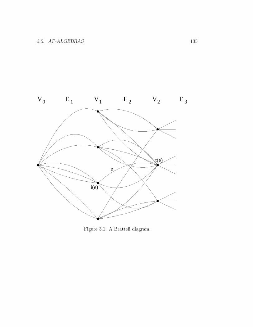
3.5. AF-ALGEBRAS 135
V E1E0V 3E
t(e)
i(e)
e
2V1 2
Figure 3.1: A Bratteli diagram.
136 CHAPTER 3. GROUPOID C∗-ALGEBRAS
1. d is a metric on XE.
2. For x in XE, we have
B(x, 21−N) = C(x1, . . . , xN).
3. For p, q in E0,N , C(p) and C(q) are equal when p = q and are disjointotherwise.
4. For p in E0,N , C(p) is clopen. (That is, C(p) is both closed and open.)
5. The collection PN = {C(p) | p ∈ E0,N} is a partition of XE intopairwise disjoint clopen sets.
6. For p in E0,N , we have
C(p) = ∪i(e)=t(p)C(pe).
7. Each element of PN+1 is contained in a single element of PN .
8. The collection ∪M≥1PM is a base for the topology of (XE, d).
9. The space XE is compact.
We leave the proof as an exercise for the interested reader. Almost all ofthis is quite easy, with the possible exception of the last part.
Having defined our space XE, we are now ready to provide an equivalencerelation on it. Of course, an equivalence relation is an example of a groupoid.More than that, this will come equipped with a topology in which it is etale.
Definition 3.5.4. Let (V,E) be a Bratteli diagram.
1. For each N ≥ 1, v in VN and pair p, q in E0,N with t(p) = t(q) = v, wedefine
γ(p, q) = {(x, y) ∈ XE ×XE | x ∈ C(p), y ∈ C(q), xn = yn, n > N}.
2. We let ΓE,v denote the collection of all such γ(p, q) with t(p) = t(q) = v.We also let ΓE,N denote the union of these over all v in VN and, finally,we let ΓE denote the union of these over all N ≥ 1. (Notice thatΓE,v,ΓE,N and ΓE are all collections of subsets of XE ×XE.)
3.5. AF-ALGEBRAS 137
3. We define
RE,N = ∪ΓE,N
RE = ∪ΓE.
(Notice that RE,N and RE are subsets of XE ×XE.)
We regard XE×XE as a groupoid with the usual product and involution:(x, y) · (x′, y′) is defined when y = x′ and the result is (x, y′) and (x, y)−1 =(y, x). We note that r(x, y) = (x, x) and s(x, y) = (y, y).
We summarize the properties of these sets with the following result. Allparts follow easily from the definition and we omit the proof.
Lemma 3.5.5. Let (V,E) be a Bratteli diagram.
1. If p, q, p′, q′ are in E0,N with t(p) = t(q), t(p′) = t(q′), then γ(p, q) =γ(p′, q′) if and only if (p, q) = (p′, q′) and they are disjoint otherwise.
2. If p, q are in E0,N with t(p) = t(q), then γ(p, q) ⊆ ∆XE if p = q andγ(p, q) ∩∆XE = ∅ if p 6= q.
3. If p, q, p′, q′ are in E0,N with t(p) = t(q), t(p′) = t(q′), then γ(p, q) ·γ(p′, q′) = γ(p, q′) if q = p′ and is empty otherwise. In the first case,the product is a bijection
4. If p, q are in E0,N with t(p) = t(q), then γ(p, q)−1 = γ(q, p).
5. If p, q are in E0,N with t(p) = t(q), then r(γ(p, q)) = γ(p, p) and r isa bijection between these two sets in XE ×XE. Similarly, s(γ(p, q)) =γ(q, q) and r is a bijection between these two sets in XE ×XE.
6. If p, q are in E0,N with t(p) = t(q), then for any M > N ,
γ(p, q) = ∪γ(pp′, qp′),
where the union is over all p′ in EN,M with i(p′) = t(p).
Again, we omit the proof since all parts are quite easy. The importancethough is summarized in the following result.
Theorem 3.5.6. Let (V,E) be a Bratteli diagram.
138 CHAPTER 3. GROUPOID C∗-ALGEBRAS
1. The set RE ⊆ XE×XE is an equivalence relation. In other words, withthe usual product from XE×XE, the set RE is a principal subgroupoid.
2. The collection of subsets ΓE forms a neighbourhood base for a topologyon RE in which it is an etale groupoid.
3. On each element of ΓE, the relative topology from the last part agreeswith the relative topology as a subset of XE ×XE.
4. Each element of ΓE is a compact, open RE-set.
Proof. It is clear that for any fixed N , the union of all sets γ(p, p), with p inE0,N is exactly ∆XE and it follows that RE is reflexive. RE is symmetric bypart 4 of Lemma 3.5.5 and transitive from part 3 of Lemma 3.5.5. Thus, RE
is an equivalence relation.The collection of sets ΓE,N is closed under intersections by part 1 of 3.5.5.
The same is true of ΓE using this fact and part 6 of 3.5.5. This immediatelyimplies that ΓE is a neighbourhood base for a topology.
The fact that the product and inverse are continuous in this topologyfollows from parts 3 and 4 of Lemma 3.5.5. The facts that both r and sare open and local homeomorphisms follows from part 5. Thus, with thetopology induced by ΓE, RE is an etale groupoid.
If we fix p, q in E0,N with t(p) = t(q), then the relative topology on γ(p, q),from our base is generated by sets γ(p′, q′) with p′, q′ in E0,N ′ with N ′ > N ,(p′1, . . . , p
′N) = p, (q′1, . . . , q
′N) = q, and (p′N+1, . . . , p
′N ′) = (q′N+1, . . . , q
′N ′). It
is a simple matter to see that
γ(p′, q′) = γ(p, q) ∩ C(p′)× C(q′).
This implies that the relative topology on γ(p, q) induced by ΓE is the sameas the product topology.
We have already seen that γ(p, q) is an open RE-set. The fact it is com-pact follows from the last statement and the fact that C(p) and C(q) areboth closed and hence compact in XE.
Definition 3.5.7. The etale groupoid RE arising from a Bratteli diagram(V,E) as above is called an AF-groupoid.
We now move on to investigate the associated groupoid C∗-algebras.
3.5. AF-ALGEBRAS 139
Definition 3.5.8. For each pair p, q in E0,N with t(p) = t(q), we definee(p, q) to be the characteristic function of γ(p, q), which lies in Cc(RE).
Lemma 3.5.9. 1. If p, q are in E0,N with t(p) = t(q), then e(p, q)∗ =e(q, p).
2. If p, q, p′, q′ are in E0,N with t(p) = t(q) 6= t(p′) = t(q′), then e(p, q)e(p′, q′) =0.
3. If p, q, p′, q′ are in E0,N with t(p) = t(q) = t(p′) = t(q′), then e(p, q)e(p′, q′) =e(p, q′) if q = p′ and is zero if q 6= p′.
4. If p, q are in E0,N with t(p) = t(q), then
e(p, q) =∑
i(e)=t(p)
e(pe, qe).
Proof. The first part is a general fact that for a compact open G-set U ,χ∗U = χU−1 combined with part 4 of 3.5.5.
Now consider the case t(p) = t(q), t(p′) = t(q′) and q 6= p′. We compute
(e(p, q)e(p′, q′)) (x, y) =∑
(x,z)∈RE
e(p, q)(x, z)e(p′, q′)(z, y).
To obtain something other than zero, we would need to find a z with(z1, . . . , zN) = q and (z1, . . . , zN) = p′. As q 6= p′ there are no such z. Thisproves part 2 and the second statement of part 3.
For the other statement of part 3, we use the same formula above. For afixed x, y, to obtain something other than zero, we must findz = (p′1, . . . , p
′N , xN+1, xN+2, . . .) for the first term to be non-zero and
z = (q1, . . . , qN , yN+1, yN+2, . . .). This requires xn = yn for all n > N andin this case, there is a unique such z and the value of e(p, q)e(p′, q′)(x, y) isone. This means that e(p, q)e(p′, q′) is the characteristic function of γ(p, q′)as claimed.
The last part follows from the last part of 3.5.5.
Theorem 3.5.10. Let (V,E) be a Bratteli diagram.
1. For a fixed vertex v in VN ,
Av = span{e(p, q) | p, q ∈ E0,N , t(p) = t(q) = v}
140 CHAPTER 3. GROUPOID C∗-ALGEBRAS
is a C∗-subalgebra of C∗(RE) and is isomorphic to Mn(v)(C), where
n(v) = #{p ∈ E0,N | t(p) = v},
the number of paths from v0 to v.
2. For a fixed positive integer N ,
AN = span{e(p, q) | p, q ∈ E0,N , t(p) = t(q)}
is a unital C∗-subalgebra of C∗(RE) and equals ⊕v∈VNAv.
3. For a fixed positive integer N , AN is a unital C∗-subalgebra of AN+1.
4. ∪N≥1AN is a dense unital ∗-subalgebra of C∗(RE).
5. The full and reduced groupoid C∗-algebras of RE are the same.
Proof. The first statement follows from parts 1 and 3 of Lemma 3.5.9 andexercise 1.7.1. If v, w are distinct vertices in VN , then Av · Aw = 0 followsfrom part 2 of Lemma 3.5.9 and the second part follows at once.
It is easy to see that, for any N ,∑
p∈E0,Ne(p, p) = χ∆XE
= ∆(1) is the
unit for Cc(RE). The fact that AN is a subalgebra of AN+1 follows from part4 of Lemma 3.5.9.
The proof of part 4 is as follows. First, we have a neighbourhood base forRE consisting of compact open sets which is also closed under intersections.It follows that every continuous function of compact support of RE can beuniformly approximated by a linear combination of such functions. Thelinear span of these functions is exactly ∪N≥1AN . This implies that thesetwo subsets will have the same completion in the C∗-algebra norm.
As each ∗-subalgebra AN in Cc(RE) is finite dimensional, it has a uniquenorm in which it is a C∗-algebra. Thus the norm on Cc(RE) in which itscompletion is a C∗-algebra is unique on the dense set ∪NAN and hence isunique. It follows that ‖ · ‖ and ‖ · ‖r agree and C∗(RE) = C∗r (RE).
Exercise 3.5.1. Let (V,E) be a Bratteli diagram. Let (xk, yk), k ≥ 1 and(x, y) be in RE. (That is, each xk and yk is an infinite sequence in XE.)Prove that the sequence (xk, yk), k ≥ 1 converges to (x, y) in R if and onlyit converges in X × X and there exists N ≥ 1 such that RE,N contains thesequence and its limit point.
3.5. AF-ALGEBRAS 141
Exercise 3.5.2. Consider the Bratteli diagram (V,E) with
1. Vn = {vn, wn}, n ≥ 1,
2. there is one edge from v0 to v1 and one edge from v0 to w1,
3. for n ≥ 1, there is one edge from vn to vn+1, one edge from vn to wn+1,and one edge from wn to wn+1.
Give a simple concrete description of X (as a familiar space) and R. Also,find a set that is open in R and not open in the relative topology on R fromX ×X.
Exercise 3.5.3. Suppose that (V,E) has full edge connections. Prove thatevery equivalence class in R is dense in X. Describe all ideals in C∗(RE).
Exercise 3.5.4. Find a necessary and sufficient condition on a Bratteli di-agram (V,E) such that C∗(RE) is commutative.
Exercise 3.5.5. Let (V,E) be a Bratteli diagram. Use the following twofacts: any finitely additive, probability measure on the clopen subsets of atotally disconnected compact space will extend to a probability measure, andthat a probability measure on such a space is uniquely determined by its re-striction to the clopen sets.
Find a bijection between the set of RE-invariant probability measures onXE and the set of all functions ν : V → [0, 1] such that
1. ν(v0) = 1,
2.ν(v) =
∑e∈En+1,i(e)=v
ν(t(e)),
for every n ≥ 0, v in Vn.
Exercise 3.5.6. Consider the following three Bratteli diagrams.
1. The diagram described in Exercise 3.5.2.
2. The diagram with exactly one vertex and exactly two edges at each level.
3. With the same vertex set as Exercise 3.5.2, have one edge from vn tovn+1, one from vn to wn+1 and one from wn to vn+1.
In each case, find all traces on the C∗-algebras of the Bratteli diagrams.