lecture 5 - national tsing hua university
TRANSCRIPT
Lecture 5Continuous Random VariablesBMIR Lecture Series in Probability and Statistics
Ching-Han Hsu, BMES, National Tsing Hua Universityc©2015 by Ching-Han Hsu, Ph.D., BMIR Lab
5.1
1 Uniform Distribution
Continuous Uniform Distribution
Definition 1 (Continuous Uniform Distribution). A continuous random variableX with probability density function
f (x) =1
b−a, a≤ x≤ b (1)
is a continuous uniform random variable.
• The mean of X is
E(X) =∫ b
a
xb−a
dx =x2
2(b−a)
∣∣∣∣ba=
a+b2
• The variance is
V (X) =∫ b
a
(x− a+b
2
)2
b−adx =
(x− a+b
2
)3
3(b−a)
∣∣∣∣∣b
a
=(b−a)2
12
5.2
CDF: Continuous Uniform Distribution
• The cumulative distribution function of a continuous uniform distributionX is
F(X) = P(X ≤ x) =∫ x
−∞
f (t)dt =∫ x
−∞
1b−a
dt. (2)
• If a≤ x≤ b,
F(X) =∫ x
a
1b−a
dt = (x−a)/(b−a). (3)
• The complete form is
F(X) =∫ x
−∞
1b−a
dt =
0 x < ax−ab−a a≤ x < b1 b≤ x
(4)
5.3
1

Probability and Statistics 2/19 Fall, 2014
Example: Continuous Uniform Distribution
Example 2. Let continuous random variable X denote the current measured in athin copper in milliamperes (mA). Assume that the range of X is [0,20mA], andthe probability density function is f (x) = 1
20−0 = 0.05, 0≤ x≤ 20.
• The mean of X is E(X) =∫ 20
0x
20dx = 202 = 10mA
• The variance is
V (X) =∫ 20
0
(x−10)2
20dx =
(20)2
12= 33.33mA2
• What is the probability that a measurement of current is between 5 and 10mA? P(5 < x≤ 10) =?
P(5 < x≤ 10) = F(10)−F(5) =1020− 5
20= 0.25
5.4
2 Normal Distribution
Normal (Gaussian) Distribution
• Normal distribution is the most widely used model.• For a repeated random experiment, the average of the outcomes tends to
have a normal distribution (central limit theorem).• The density function of a normal random variable is characterized by two
parameters: mean µ and variance σ2 as shown in Fig. 1.• Each curve is symmetric and bell-shaped.• µ determines the center and σ2 determines the width.
5.5
Normal (Gaussian) Distribution
Figure 1: Normal probability density functions for selected values of the param-eters µ and σ2.
5.6
BMES, NTHU. BMIR c©Ching-Han Hsu, Ph.D.
Probability and Statistics 3/19 Fall, 2014
Normal (Gaussian) Distribution
Definition 3 (Normal (Gaussian) Distribution). A continuous random variable Xwith probability density function
f (x; µ,σ) =1√
2πσ2e−
(x−µ)2
2σ2 , −∞ < x < ∞ (5)
=1
σ√
2πe−
(x−µ)2
2σ2 , −∞ < x < ∞ (6)
is a normal (Gaussian) random variable with parameters µ , where −∞ < µ < ∞,and σ > 0.
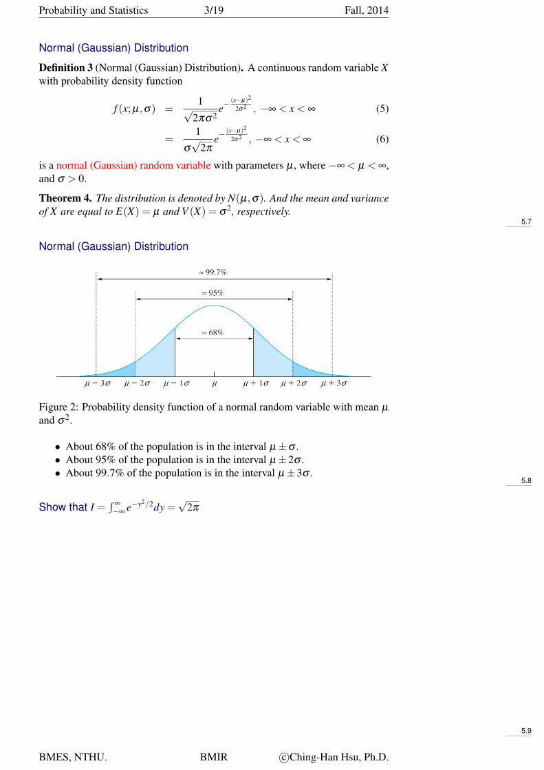
Theorem 4. The distribution is denoted by N(µ,σ). And the mean and varianceof X are equal to E(X) = µ and V (X) = σ2, respectively.
5.7
Normal (Gaussian) Distribution
Figure 2: Probability density function of a normal random variable with mean µ
and σ2.
• About 68% of the population is in the interval µ±σ .• About 95% of the population is in the interval µ±2σ .• About 99.7% of the population is in the interval µ±3σ .
5.8
Show that I =∫
∞
−∞e−y2/2dy =
√2π
I2 =∫
∞
−∞
e−x2/2dx ·∫
∞
−∞
e−y2/2dy
=∫
∞
−∞
∫∞
−∞
e−(x2+y2)/2dxdy
=∫
∞
0
∫ 2π
0e−r2/2rdrdθ (dxdy = rdrdθ)
=∫ 2π
0dθ ·
∫∞
0e−r2/2rdr
= 2π ·∫
∞
0e−r2/2d
r2
2(r2/2 = s)
= 2π
∫∞
0e−sds = 2π
I =√
2π =∫
∞
−∞
e−y2/2dy
5.9
BMES, NTHU. BMIR c©Ching-Han Hsu, Ph.D.

Probability and Statistics 4/19 Fall, 2014
Mean and Variance of Normal Random VariableShow that E(X) = µ .
E(X) =∫
∞
−∞
x1
σ√
2πe−
(x−µ)2
2σ2 dx (y = (x−µ)/σ)
=∫
∞
−∞
1√2π
(σy+µ)e−y2/2dy
=∫
∞
−∞
σ√2π
ye−y2/2dy+∫
∞
−∞
µ1√2π
e−y2/2dy
= 0+µ1√2π
∫∞
−∞
e−y2/2dy
= µ
Show that V (X) = σ2. 5.10
Standard Normal Random Variable
Definition 5 (Standard Normal Random Variable). A normal random variablewith µ = 0 and σ = 1, N(0,1), is called a standard normal random variable andis denoted as Z.
Definition 6 (Standard Normal Random Variable). The cumulative distributionfunction of a standard normal random variable is denoted as
Φ(z) = P(Z ≤ z)5.11
Standardized Normal Random Variable
Definition 7 (Standardized Normal Random Variable). If X is a normal randomvariable N(µ,σ), the random variable
Z =X−µ
σ(7)
is a normal random variable N(0,1). That is, Z is a standard normal randomvariable. Also,
P(X ≤ x) = P(
X−µ
σ≤ x−µ
σ
)= P(Z ≤ z) (8)
wherez =
x−µ
σ(9)
is the z−value (or z−score ) obtained by standardizing X .5.12
Example: Standard Normal DistributionExample 8. Aluminum sheets used to make beverage cans have thicknesses (inthousandths of an inch) that are normally distributed with mean 10 and standarddeviation 1.3. A particular sheet is 10.8 thousandths of an inch thick. Find thez-score.
The quantity 10.8 is an observation from a normal population with meanµ = 10 and standard deviation σ = 1.3. Therefore
z =x−µ
σ=
10.8−101.3
= 0.62
5.13
BMES, NTHU. BMIR c©Ching-Han Hsu, Ph.D.
Probability and Statistics 5/19 Fall, 2014
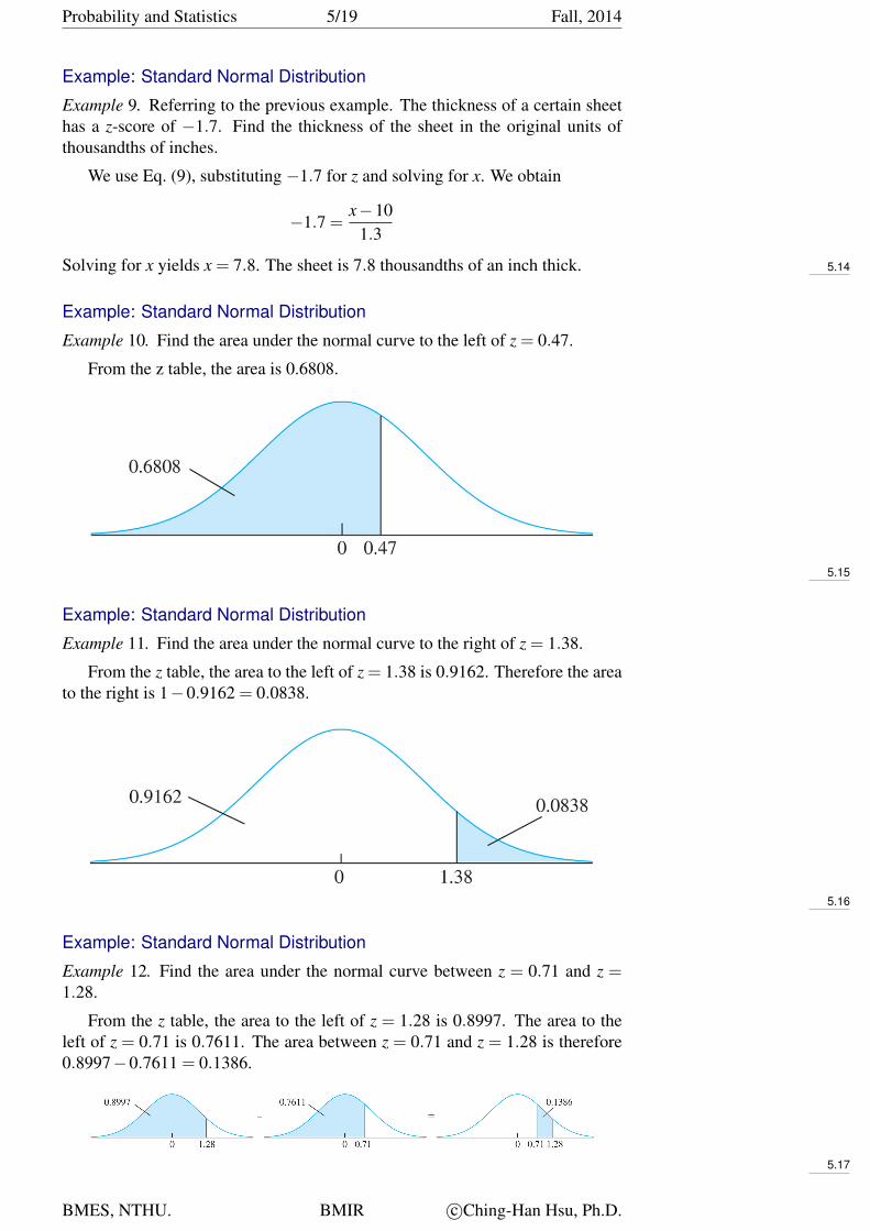
Example: Standard Normal Distribution
Example 9. Referring to the previous example. The thickness of a certain sheethas a z-score of −1.7. Find the thickness of the sheet in the original units ofthousandths of inches.
We use Eq. (9), substituting −1.7 for z and solving for x. We obtain
−1.7 =x−10
1.3
Solving for x yields x = 7.8. The sheet is 7.8 thousandths of an inch thick. 5.14
Example: Standard Normal Distribution
Example 10. Find the area under the normal curve to the left of z = 0.47.
From the z table, the area is 0.6808.
5.15
Example: Standard Normal Distribution
Example 11. Find the area under the normal curve to the right of z = 1.38.
From the z table, the area to the left of z = 1.38 is 0.9162. Therefore the areato the right is 1−0.9162 = 0.0838.
5.16
Example: Standard Normal Distribution
Example 12. Find the area under the normal curve between z = 0.71 and z =1.28.
From the z table, the area to the left of z = 1.28 is 0.8997. The area to theleft of z = 0.71 is 0.7611. The area between z = 0.71 and z = 1.28 is therefore0.8997−0.7611 = 0.1386.
5.17
BMES, NTHU. BMIR c©Ching-Han Hsu, Ph.D.
Probability and Statistics 6/19 Fall, 2014
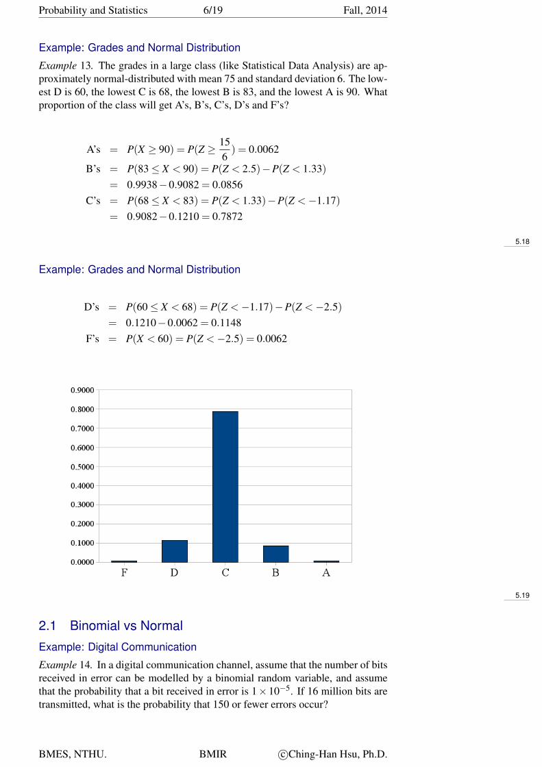
Example: Grades and Normal Distribution
Example 13. The grades in a large class (like Statistical Data Analysis) are ap-proximately normal-distributed with mean 75 and standard deviation 6. The low-est D is 60, the lowest C is 68, the lowest B is 83, and the lowest A is 90. Whatproportion of the class will get A’s, B’s, C’s, D’s and F’s?
A’s = P(X ≥ 90) = P(Z ≥ 156) = 0.0062
B’s = P(83≤ X < 90) = P(Z < 2.5)−P(Z < 1.33)= 0.9938−0.9082 = 0.0856
C’s = P(68≤ X < 83) = P(Z < 1.33)−P(Z <−1.17)= 0.9082−0.1210 = 0.7872
5.18
Example: Grades and Normal Distribution
D’s = P(60≤ X < 68) = P(Z <−1.17)−P(Z <−2.5)= 0.1210−0.0062 = 0.1148
F’s = P(X < 60) = P(Z <−2.5) = 0.0062
5.19
2.1 Binomial vs Normal
Example: Digital Communication
Example 14. In a digital communication channel, assume that the number of bitsreceived in error can be modelled by a binomial random variable, and assumethat the probability that a bit received in error is 1×10⁻⁵. If 16 million bits aretransmitted, what is the probability that 150 or fewer errors occur?
BMES, NTHU. BMIR c©Ching-Han Hsu, Ph.D.
Probability and Statistics 7/19 Fall, 2014
Let X denote the number of errors. Then X is a binomial random variable.And
P(X ≤ 150) =150
∑0
(16000000
x
)(10−5)x(1−10−5)16000000−x
How to compute this equation?. 5.20
Approximation of Binomial Distribution
Theorem 15. If X is a binomial random variable with parameters n and p
Z =X−np√np(1− p)
(10)
is approximately a standard normal random variable. To approximate a bino-mial probability with a normal distribution a continuity correction is applied asfollows:
P(X ≤ x) = P(X ≤ x+0.5) = P
(Z ≤ x+0.5−np√
np(1− p)
)(11)
P(x≤ X) = P(x−0.5≤ X) = P
(x−0.5−np√
np(1− p)≤ Z
)(12)
This approximation is good for np > 5 and n(1− p)> 5.5.21
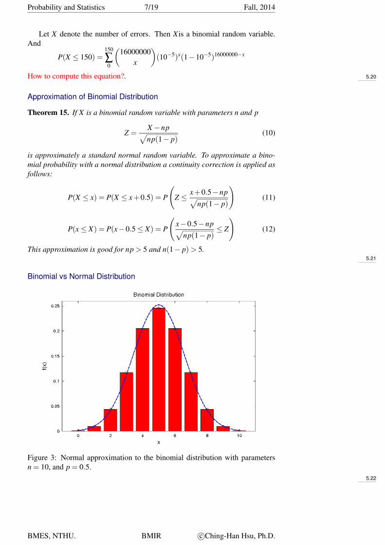
Binomial vs Normal Distribution
Figure 3: Normal approximation to the binomial distribution with parametersn = 10, and p = 0.5.
5.22
BMES, NTHU. BMIR c©Ching-Han Hsu, Ph.D.

Probability and Statistics 8/19 Fall, 2014
Example: Digital Communication (cont)
• Since np = (16×106)(1×10⁻⁵) = 160 > 5 and n(1− p)> 5, we can usethe normal distribution to approximate the original binomial distributionas:
P(X ≤ 150) = P(X ≤ 150+0.5)
= P
(X−160√
160(1−10−5)≤ 150.5−160√
160(1−10−5)
)= P(Z ≤−0.75) = 0.227
5.23
Non-symmetric Binomial vs Normal Distribution
Figure 4: Binomial distribution is not symmetric if p is close to 0 or 1. (If npor n(1− p) is small, the binomial is quite skewed and the symmetric normaldistribution is not a good approximation. )
5.24
2.2 Poisson vs Normal
Approximation of Poisson Distribution
Theorem 16. If X is a Poisson random variable with E(X) = λ and V (X) = λ ,
Z =X−λ√
λ(13)
is approximately a standard normal distribution. This approximation is good forλ > 5.
5.25
Poisson Distribution with Small λ 5.26
Poisson Distribution with Large λ 5.27
BMES, NTHU. BMIR c©Ching-Han Hsu, Ph.D.
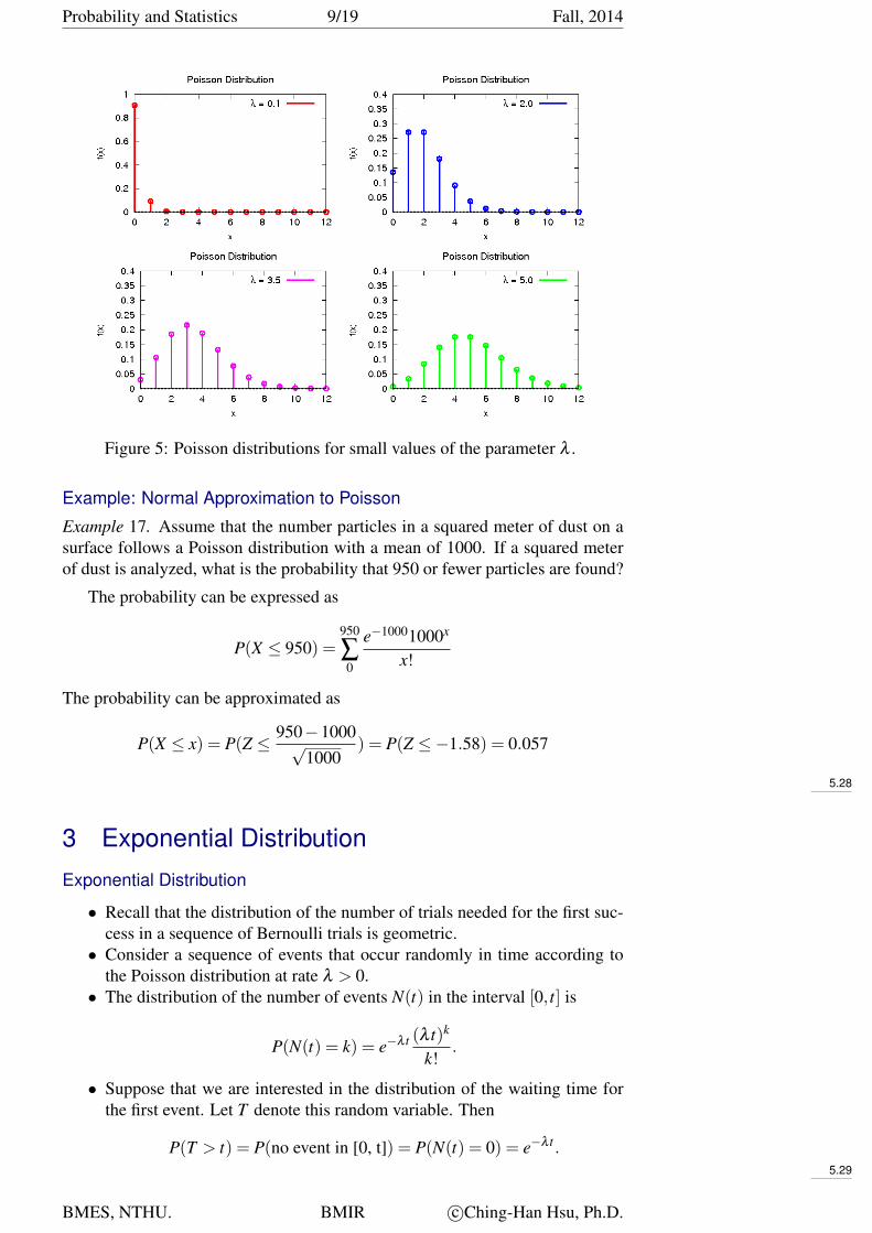
Probability and Statistics 9/19 Fall, 2014
Figure 5: Poisson distributions for small values of the parameter λ .
Example: Normal Approximation to Poisson
Example 17. Assume that the number particles in a squared meter of dust on asurface follows a Poisson distribution with a mean of 1000. If a squared meterof dust is analyzed, what is the probability that 950 or fewer particles are found?
The probability can be expressed as
P(X ≤ 950) =950
∑0
e−10001000x
x!
The probability can be approximated as
P(X ≤ x) = P(Z ≤ 950−1000√1000
) = P(Z ≤−1.58) = 0.057
5.28
3 Exponential Distribution
Exponential Distribution
• Recall that the distribution of the number of trials needed for the first suc-cess in a sequence of Bernoulli trials is geometric.• Consider a sequence of events that occur randomly in time according to
the Poisson distribution at rate λ > 0.• The distribution of the number of events N(t) in the interval [0, t] is
P(N(t) = k) = e−λ t (λ t)k
k!.
• Suppose that we are interested in the distribution of the waiting time forthe first event. Let T denote this random variable. Then
P(T > t) = P(no event in [0, t]) = P(N(t) = 0) = e−λ t .5.29
BMES, NTHU. BMIR c©Ching-Han Hsu, Ph.D.
Probability and Statistics 10/19 Fall, 2014
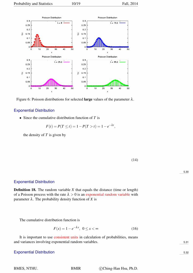
Figure 6: Poisson distributions for selected large values of the parameter λ .
Exponential Distribution
• Since the cumulative distribution function of T is
F(t) = P(T ≤ t) = 1−P(T > t) = 1− e−λ t ,
the density of T is given by
f (t) =ddt
F(t) =− ddt
P(T > t)
=
{λe−λ t , fort ≥ 00, fort < 0
. (14)
5.30
Exponential Distribution
Definition 18. The random variable X that equals the distance (time or length)of a Poisson process with the rate λ > 0 is an exponential random variable withparameter λ . The probability density function of X is
f (x) = λe−λx, 0≤ x < ∞ (15)
The cumulative distribution function is
F(x) = 1− e−λx, 0≤ x < ∞ (16)
It is important to use consistent units in calculation of probabilities, meansand variances involving exponential random variables. 5.31
Exponential Distribution 5.32
BMES, NTHU. BMIR c©Ching-Han Hsu, Ph.D.
Probability and Statistics 11/19 Fall, 2014
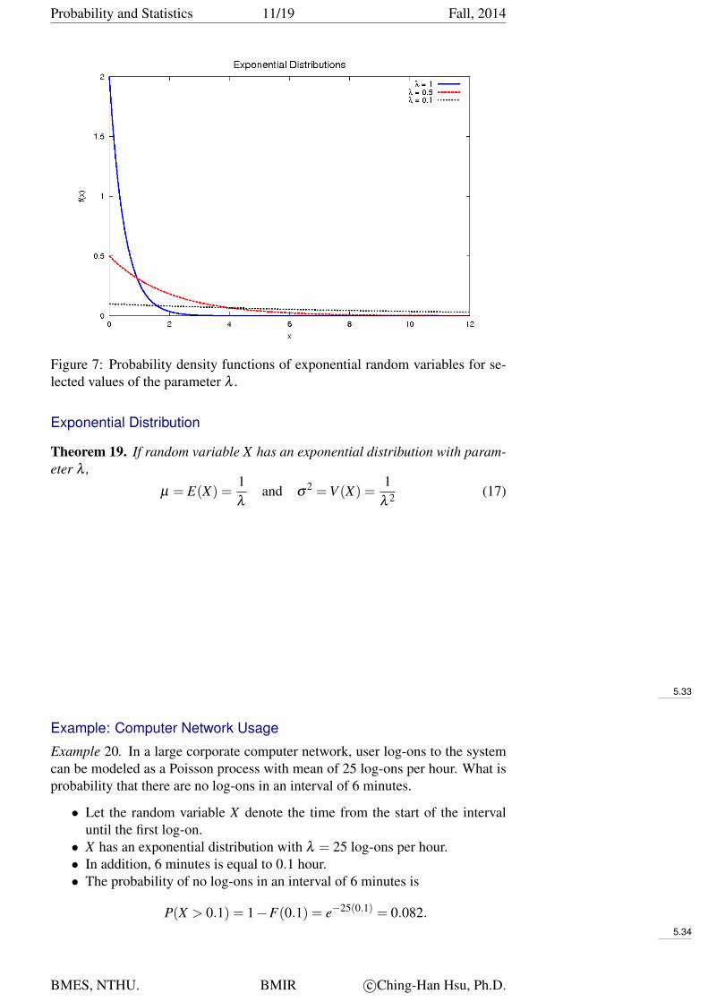
Figure 7: Probability density functions of exponential random variables for se-lected values of the parameter λ .
Exponential Distribution
Theorem 19. If random variable X has an exponential distribution with param-eter λ ,
µ = E(X) =1λ
and σ2 =V (X) =
1λ 2 (17)
µ = E(X) =∫
∞
0xλe−λxdx
=∫
∞
0xe−λxdλx =−
∫∞
0xde−λx
=(−xe−λx
)∣∣∣∞0+∫
∞
0e−λxdx
= − 1λ
e−λx∣∣∣∣∞0= 0− −1
λ=
1λ
5.33
Example: Computer Network Usage
Example 20. In a large corporate computer network, user log-ons to the systemcan be modeled as a Poisson process with mean of 25 log-ons per hour. What isprobability that there are no log-ons in an interval of 6 minutes.
• Let the random variable X denote the time from the start of the intervaluntil the first log-on.• X has an exponential distribution with λ = 25 log-ons per hour.• In addition, 6 minutes is equal to 0.1 hour.• The probability of no log-ons in an interval of 6 minutes is
P(X > 0.1) = 1−F(0.1) = e−25(0.1) = 0.082.5.34
BMES, NTHU. BMIR c©Ching-Han Hsu, Ph.D.
Probability and Statistics 12/19 Fall, 2014
Example: Computer Network Usage
• What is probability that the time until next log-on is between 2 and 3 min-utes
P(
260
= 0.033 < X <3
60= 0.05
)= F(0.05)−F(0.033) = e−25(0.05)e−25(0.033)
= 0.152.
• The mean time until the next log-on is
µ =1λ=
125
= 0.04 hr = 2.4 min
• The standard deviation of the time until the next log-on is mean time untilthe next log-on is
σ =1
25hr = 2.4 min
5.35
Example: Lack of Memory
Example 21. Let X denote the time between detections of a particle with a Geigercounter. Assume that X has an exponential distribution with E(X) = 1.4 minutes.
• The probability that we detect a particle within 30 seconds of starting thecounter is
P(X < 0.5 min) = F(0.5) = 1− e−0.5/1.4 = 0.30.
• Suppose that the counter has been on for 3 minutes without detecting aparticle. What is the probability that we detect a particle in next 30 sec-onds:
P(X < 3.5|X > 3) = P(3 < X < 3.5)/P(X > 3)5.36
Example: Lack of Memory
• We have
P(3 < X < 3.5) = F(3.5)−F(3) = 0.035P(X > 3) = 1−F(3) = 0.117
P(X < 3.5|X > 3) = P(3 < X < 3.5)/P(X > 3)= 0.035/0.117 = 0.30
• After waiting for 3 minutes without a detection, the probability of a detec-tion in next 30 seconds is the same as the probability of a detection in the30 seconds immediately after starting the counter.
Theorem 22 (Lack of Memory). For an exponential random variable X
P(X < (t1 + t2)|X > t1) = P(X < t2) (18)5.37
BMES, NTHU. BMIR c©Ching-Han Hsu, Ph.D.
Probability and Statistics 13/19 Fall, 2014
4 Erlang and Gamma Distributions
Example: Erlang DistributionExample 23 (CPU Failure). The failure of the CPUs of large computer systemsare often modeled as a Poisson process. Assume that the units that fail are imme-diately repaired, and assume that the mean number of failure per hour is 0.0001.Let X denote the time until four failures occur in a system. Determine the prob-ability that X exceeds 40,000 hours.
• Let the random variable N denote the number of failures in 40,000 hours.• The time until four failures occur exceeds 40,000 hours if the number of
failures in 40,000 hours in three or less:
P(X > 40,000) = P(N ≤ 3)5.38
Example: Erlang Distribution• N has a Poisson distribution with
E(N) = 40,000(0.0001) = 4 failures in 40,000 hours
• Therefore,
P(X > 40,000) = P(N ≤ 3) =3
∑k=0
e−44k
k!= 0.433
5.39
Erlang Distribution• If X is the time until the rth event in a Poisson process then
P(X > x) =r−1
∑k=0
e−λx(λx)k
k!
• Since P(X > x) = 1−F(X), the probability density function of X equals
f (x) =− ddx
P(X > x) =λ rxr−1e−λx
(r−1)!
for x > 0 and r = 1,2, . . ..• This probability density function defines an Erlang distribution.• With r = 1, an Erlang RV becomes an exponential RV.
5.40
Gamma Function
Definition 24 (Gamma Function). The gamma function of γ is
Γ(γ) =∫
∞
0xγ−1e−xdx, for γ > 0. (19)
• The value of the integral is a positive finite number.• Using the integral by parts, it can be shown that
Γ(γ) = (γ−1)Γ(γ−1)
• If γ is a positive integer, (as in Erlang distribution), Γ(γ) = (γ−1)!, giventhat γ(1) = 0! = 1.• β γΓ(γ) =
∫∞
0 yγ−1e−y/β dy.5.41
BMES, NTHU. BMIR c©Ching-Han Hsu, Ph.D.
Probability and Statistics 14/19 Fall, 2014
Gamma Distribution
Definition 25 (Gamma Distribution). A random variable X that has a pdf
f (x;γ,λ ) =
{λ γ xγ−1e−λx
Γ(γ) = λ
Γ(γ)(λx)γ−1e−λx, 0 < x < ∞
0, elsewhere. (20)
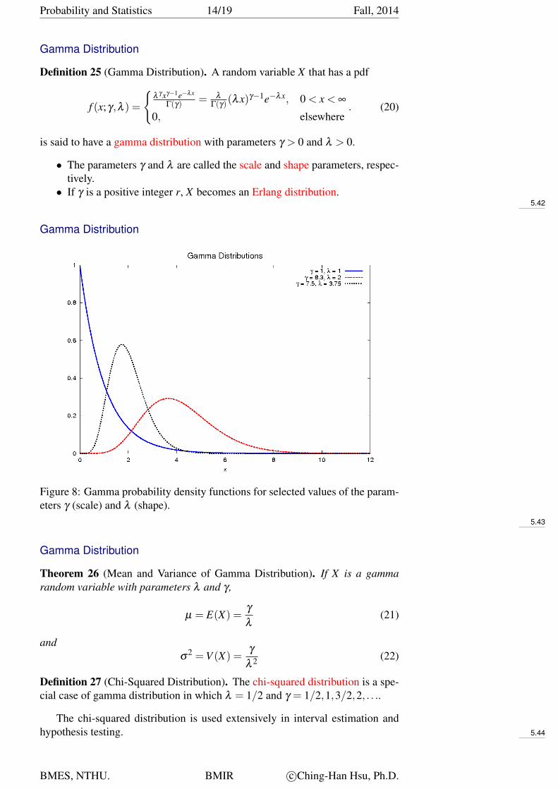
is said to have a gamma distribution with parameters γ > 0 and λ > 0.
• The parameters γ and λ are called the scale and shape parameters, respec-tively.• If γ is a positive integer r, X becomes an Erlang distribution.
5.42
Gamma Distribution
Figure 8: Gamma probability density functions for selected values of the param-eters γ (scale) and λ (shape).
5.43
Gamma Distribution
Theorem 26 (Mean and Variance of Gamma Distribution). If X is a gammarandom variable with parameters λ and γ ,
µ = E(X) =γ
λ(21)
andσ
2 =V (X) =γ
λ 2 (22)
Definition 27 (Chi-Squared Distribution). The chi-squared distribution is a spe-cial case of gamma distribution in which λ = 1/2 and γ = 1/2,1,3/2,2, . . ..
The chi-squared distribution is used extensively in interval estimation andhypothesis testing. 5.44
BMES, NTHU. BMIR c©Ching-Han Hsu, Ph.D.
Probability and Statistics 15/19 Fall, 2014
Example: Gamma Distribution
Example 28. The time to prepare a micro-array slide for high throughput ge-nomics is a Poisson process with a mean of two hours per slide. What is theprobability that 10 slides require more than 25 hours to prepare?
• Let X denote the time to prepare 10 slides.• X has gamma distribution with λ = 1/2 (slide/hour) and γ = 10.• Th requested probability P(X > 25)
P(X > 25) =9
∑k=0
e−12.5(12.5)k
k!= 0.2014
• The mean time to prepare 10 slides is E(X) = γ/λ = 10/0.5 = 20 hours.And the variance time is V (X) = γ/λ 2 = 40
5.45
5 Weibull Distribution
Weibull Distribution
Definition 29 (Weibull Distribution). The random variable X with the probabil-ity density function
f (x) =β
δ
( xδ
)β−1exp[−( x
δ
)β], x > 0 (23)
is a Weibull random variable with scale parameter δ > 0 and shape parameterβ > 0.
• The Weibull distribution is often used to model the time until failure ofmany different physical systems.• When β = 1, the Weibull distribution is identical to the exponential.• The Raleigh distribution is a special case when the shape parameter β = 2.
5.46
Weibull Distribution 5.47
Weibull Distribution
Theorem 30. If X has a Weibull distribution with parameters δ and β , then thecumulative distribution function of X is
F(x) = 1− exp[−( x
δ
)β]
(24)
Theorem 31. If X has a Weibull distribution with parameters δ and β ,
µ = E(X) = δΓ
(1+
1β
)(25)
σ2 =V (X) = δ
2Γ
(1+
2β
)−δ
2[
Γ
(1+
1β
)]2
(26)
5.48
BMES, NTHU. BMIR c©Ching-Han Hsu, Ph.D.
Probability and Statistics 16/19 Fall, 2014
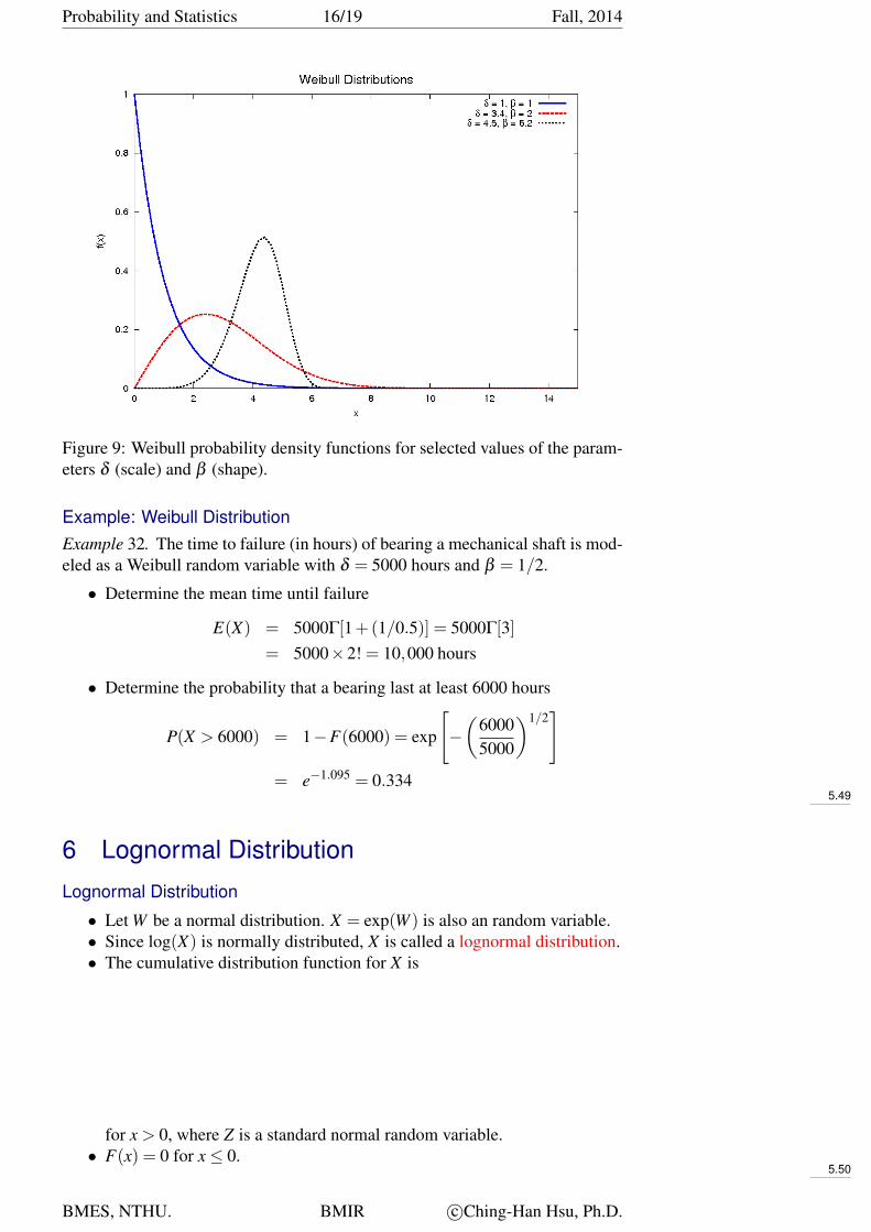
Figure 9: Weibull probability density functions for selected values of the param-eters δ (scale) and β (shape).
Example: Weibull DistributionExample 32. The time to failure (in hours) of bearing a mechanical shaft is mod-eled as a Weibull random variable with δ = 5000 hours and β = 1/2.
• Determine the mean time until failure
E(X) = 5000Γ[1+(1/0.5)] = 5000Γ[3]= 5000×2! = 10,000 hours
• Determine the probability that a bearing last at least 6000 hours
P(X > 6000) = 1−F(6000) = exp
[−(
60005000
)1/2]
= e−1.095 = 0.3345.49
6 Lognormal Distribution
Lognormal Distribution
• Let W be a normal distribution. X = exp(W ) is also an random variable.• Since log(X) is normally distributed, X is called a lognormal distribution.• The cumulative distribution function for X is
F(x) = P(X ≤ x)= P(exp(W )≤ x) = P(W ≤ log(x))
= P(
Z ≤ log(x)−θ
ω
)= Φ
(log(x)−θ
ω
)for x > 0, where Z is a standard normal random variable.• F(x) = 0 for x≤ 0.
5.50
BMES, NTHU. BMIR c©Ching-Han Hsu, Ph.D.

Probability and Statistics 17/19 Fall, 2014
Lognormal Distribution
Definition 33 (Lognormal Distribution). Let W have a normal distribution withmean θ and variance ω2; then X = exp(W ) is a lognormal random variable withprobability density function
f (x) =1
xω√
2πexp[−(log(x)−θ)2
2ω2
](27)
for 0 < x < ∞. The mean and variance of X are
E(X) = exp(θ +ω2/2)
V (X) = e2θ+ω2(eω2−1)
The lifetime of a product that degrades over time is often modeled by a log-normal distribution random variable. 5.51
Lognormal Distribution
Figure 10: Normal probability density functions with θ = 0 for selected valuesof σ2.
5.52
Lognormal Distribution 5.53
Lognormal Distribution 5.54
Example: Lognormal Distribution
Example 34. The lifetime of a semiconductor laser has a lognormal distributionwith θ = 10 hours and ω = 1.5 hours.
BMES, NTHU. BMIR c©Ching-Han Hsu, Ph.D.

Probability and Statistics 18/19 Fall, 2014
Figure 11: Lognormal probability density functions with θ = 0 for selected val-ues of ω2.
• What is the probability the lifetime exceeds 10,000 hours?
P(X > 10000) = 1−P(exp(W )≤ 10000)= 1−P(W ≤ log(10000))
= 1−Φ
(log(10000)−10
1.5
)= 1−Φ(−0.52) = 1−0.30 = 0.70
5.55
Example: Lognormal Distribution• What lifetime is exceeded by 99% of lasers?
P(X > x) = P(exp(W )> x) = P(W > log(x))
= 1−Φ
(log(x)−10
1.5
)= 0.99
1−Φ(z) = 0.99 when z =−2.33. Therefore,
log(x)−101.5
=−2.33
x = exp(6.505) = 668.48 hours5.56
Example: Lognormal Distribution• Determine the mean and variance of lifetime.
E(X) = exp(θ +ω2/2) = exp(10+1.125)
= 67,846.3
V (X) = e2θ+ω2(eω2−1)
= exp(20+2.25)[exp(2.25)−1]= 39,070,059,886.6
σ =√
V (x) = 197,661.5� E(X)
Notice that the standard deviation of life time is much larger to the mean. 5.57
BMES, NTHU. BMIR c©Ching-Han Hsu, Ph.D.
Probability and Statistics 19/19 Fall, 2014
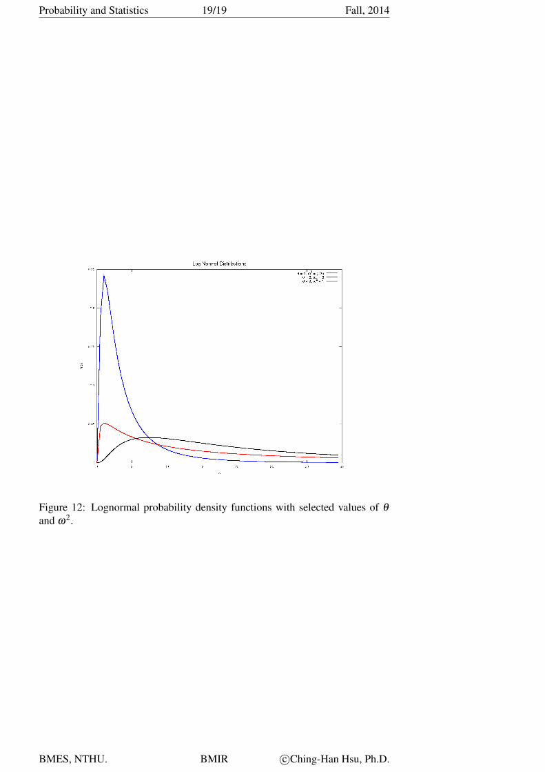
Figure 12: Lognormal probability density functions with selected values of θ
and ω2.
BMES, NTHU. BMIR c©Ching-Han Hsu, Ph.D.