lecture 4 large-scale optimization...

Lecture 4

Large-scale optimization problems

Large-scale non-smooth convex problems, complexity bounds, subgradient descent algorithm,bundle methods

4.1 Goals and motivations

We start now a new topic - complexity and efficient methods of large-scale convex optimiza-tion. Thus, we come back to problems of the type

(p) minimize f(x) s.t. gi(x) ≤ 0, i = 1, ..., m, x ∈ G,

where G is a given solid in Rn and f, g1, ..., gm are convex continuous on G functions. Thefamily of all consistent problems of the indicated type was denoted by Pm(G), and we areinterested in finding ε-solution to a problem instance from the family, i.e., a point x ∈ Gsuch that

f(x)−minGf ≤ ε(max

Gf −min

Gf), gi(x) ≤ ε(max

Ggi)+, i = 1, ..., m.

We have shown that the complexity of the family in question satisfies the inequalities

⌊O(1)n ln(1/ε)⌋ ≤ A(ε) ≤⌋2.182n ln(1/ε)⌊, (4.1.1)

where O(1) is an appropriate positive absolute constant; what should be stressed that theupper complexity bound holds true for all ε ∈ (0, 1), while the lower one is valid only for nottoo large ε, namely, for

ε < ε(G).

The ”critical value” ε(G) depends, as we remember, on affine properties of G; for the box itis 1

2, and for any n-dimensional solid G one has

ε(G) ≥ 1

2n3.

73

74 LECTURE 4. LARGE-SCALE OPTIMIZATION PROBLEMS

Thus, our complexity bounds identify complexity, up to an absolute constant factor, onlyfor small enough values of ε; there is an initial interval of values of the relative accuracy

∆(G) = [ε(G), 1)

where we to the moment have only an upper bound on the complexity and have no lowerbound. Should we be bothered by this incompleteness of our knowledge? I think we should.Indeed, what is the initial segment, it depends on G; if G is a box, then this segment isonce for ever fixed, so that there, basically, is nothing to worry about - one hardly might beinterested in solving optimization problems within relative inaccuracy ≥ 1/2, and for smallerε we know the complexity. But if G is a more general set than a box, then there is somethingto think about: all we can say about an arbitrary n-dimensional G is that ε(G) ≥ 1/(2n3);this lower bound tends to 0 as the dimension n of the problem increases, so that for large n∆(G) can in fact ”almost cover” the interval (0, 1) of all possible values of ε. On the otherhand, when solving large-scale problems of real world origin, we often are not interested intoo high accuracy, and it may happen that the value of ε we actually are interested in isexactly in ∆(G), where we do not know what is the complexity and what are the optimalmethods. Thus, we have reasons, both of theoretical and practical origin, to be interestedin the pre-asymptotic behaviour of the complexity.

The difficulty in investigating the behaviour of the complexity in the initial range ofvalues of the accuracy is that it depends on affine properties of the domain G, and this issomething too diffuse for quantitative description. This is why it is reasonable to restrictourselves with certain ”standard” domains G. We already know what happens when G is aparallelotope, or, which is the same, a box - in this case there, basically, is no initial segment.And, of course, the next interesting case is when G is an ellipsoid, or, which is the same,an Euclidean ball (all our notions are affine invariant, so to speak about Euclidean balls isthe same as to speak about arbitrary ellipsoids). This is the case we shall focus on. In factwe shall assume G to be something like a ball rather than a ball exactly. Namely, let usfix a real α ≥ 1 and assume that the asphericity of G is at most α, i.e., there is a pair ofconcentric Euclidean balls Vin and Vout with the ratio of radii not exceeding α and such thatthe smaller ball is inside G, and the larger one contains G:

Vin ⊂ G ⊂ Vout.

4.2 The main result

Our main goal is to establish the following

Theorem 4.2.1 The complexity of the family Pm(G) of convex problems with m functionalconstraints on an n-dimensional domain G of asphericity α satisfies the bounds

minn, ⌊ 1

(2αε)2− 0⌋ ≤ A(ε) ≤ ⌊4α

2

ε2⌋ + 1, 0 < ε < 1; (4.2.2)

here ⌊a− 0⌋ is the largest integer which is smaller than a real a.

4.2. THE MAIN RESULT 75

Comment. Before proving the theorem, let us think what the theorem says. First, it saysthat the complexity of convex minimization on a domain similar to an Euclidean ball isbounded from above uniformly in the dimension by a function O(1)α2ε−2; the asphericity αis responsible for the level of similarity between the domain and a ball. Second, we see thatin the large-scale case, when the dimension of the domain is large enough for given α andε, or, which is the same, when the inaccuracy ε is large enough for a given dimension (andasphericity), namely, when

ε ≥ 1

2α√n, (4.2.3)

then the complexity admits a lower bound O(1)α−2ε−2 which differs from the aforementionedupper bound by factor O(1)α−4 which depends on asphericity only. Thus, in the large-scale case (4.2.3) our upper complexity bound coincides with the complexity up to a factordepending on asphericity only; if G is an Euclidean ball (α = 1), then this factor does notexceed 16.

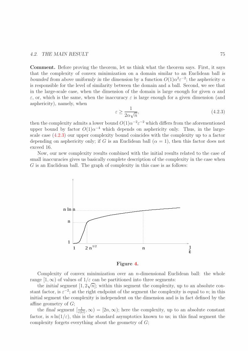
Now, our new complexity results combined with the initial results related to the case ofsmall inaccuracies gives us basically complete description of the complexity in the case whenG is an Euclidean ball. The graph of complexity in this case is as follows:

11

2 n n

n ln n

n

1/2 1-ε

Figure 4.

Complexity of convex minimization over an n-dimensional Euclidean ball: the wholerange [1,∞) of values of 1/ε can be partitioned into three segments:

the initial segment [1, 2√n]; within this segment the complexity, up to an absolute con-

stant factor, is ε−2; at the right endpoint of the segment the complexity is equal to n; in thisinitial segment the complexity is independent on the dimension and is in fact defined by theaffine geometry of G;

the final segment [ 1ε(G)

,∞) = [2n,∞); here the complexity, up to an absolute constant

factor, is n ln(1/ε), this is the standard asymptotics known to us; in this final segment thecomplexity forgets everything about the geometry of G;


the intermediate segment [2√n, 2n]; at the left endpoint of this segment the complexity

is O(n), at the right endpoint it is O(n lnn); within this segment we know complexity up toa factor of order of its logarithm rather than up to an absolute constant factor.

Now let us prove the theorem.

4.3 Upper complexity bound: Subgradient Descent

The upper complexity bound is associated with one of the most traditional methods fornonsmooth convex minimization - the short-step Subgradient Descent method. The genericscheme of the method is as follows:

given a starting point x1 ∈ intG and the required relative accuracy ε ∈ (0, 1), form thesequence

xi+1 = xi − γiRei, (4.3.4)

where γi > 0 is certain stepsize, R is the radius of the Euclidean ball Vout covering G andthe unit vector ei is defined as follows:

(i) if xi 6∈ intG, then ei is an arbitrary unit vector which separates xi and G:

(x− xi)T ei ≤ 0, x ∈ G;

(ii) if xi ∈ intG, but there is a constraint gj which is ”ε-violated” at xi, i.e., is such that

gj(xi) > ε(maxx∈G

gj(xi) + (x− xi)Tg′j(xi)

)

+, (4.3.5)

then

ei =1

|g′j(xi)|g′j(xi);

(iii) if xi ∈ intG and no constraint is ε-violated at xi, i.e., no inequality (4.3.5) is satisfied,then

ei =1

|f ′(xi)|f ′(xi).

Note that the last formula makes sense only if f ′(xi) 6= 0; if in the case of (iii) we meet withf ′(xi) = 0, then we simply terminate and claim that xi is the result of our activity.

Same as in the cutting plane scheme, let us say that search point xi is productive, if at i-thstep we meet the case (iii), and non-productive otherwise, and let us define i-th approximatesolution xi as the best (with the smallest value of the objective) of the productive searchpoints generated in course of the first i iterations (if no productive search point is generated,xi is undefined).

The efficiency of the method is given by the following.

Proposition 4.3.1 Let a problem (p) from the family Pm(G) be solved by the short-stepSubgradient Descent method associated with accuracy ε, and let N be a positive integer suchthat

2 + 12

∑Nj=1 γ

2j∑N

j=1 γj<ε

α. (4.3.6)

4.3. UPPER COMPLEXITY BOUND: SUBGRADIENT DESCENT 77

Then either the method terminates in course of N steps with the result being an ε-solutionto (p), or xN is well-defined and is an ε-solution to (p).

In particular, ifγi ≡ ε/α,

then (4.3.6) is satisfied by

N ≡ N(ε) = ⌊4α2

ε2⌋+ 1,

and with the indicated choice of the stepsizes we can terminate the method after the N-thstep; the resulting method solves any problem from the class within relative accuracy ε withthe complexity N(ε), which is exactly the upper complexity bound stated in Theorem 4.2.1.

Proof. Let me make the following crucial observation: let us associate with the method thelocalizers

Gi = x ∈ G | (x− xj)T ej ≤ 0, 1 ≤ j ≤ i. (4.3.7)

Then the presented method fits our generic cutting plane scheme for problems with functionalconstraints, up to the fact that Gi now should not necessarily be solids (they may possessempty interior or even be themselves empty) and xi should not necessarily be an interior pointof Gi−1. But all these particularities were not used in the proof of the general proposition onthe rate of convergence of the scheme (Proposition 3.3.1), and in fact there we have provedthe following:

Proposition 4.3.2 Assume that we are generating a sequence of search points xi ∈ Rn andassociate with these points vectors ei and approximate solutions xi in accordance to (i)-(iii).Let the sets Gi be defined by the pairs (xi, ei) according to (4.3.7), and let Size be a size.Assume that in course of N steps we either terminate due to vanishing of the subgradient ofthe objective at a productive search point, or this is not the case, but

Size(GN) < ε Size(G)

(if GN is not a solid, then, by definition, Size(GN) = 0). In the first case the result formedat the termination is an ε-solution to the problem; in the second case such a solution is xN(which is for sure well-defined).

Now let us apply this latter proposition to our short-step Subgradient Descent method andto the size

InnerRad(Q) = maxr | Q contains an Euclidean ball of radius r.

We know in advance that G contains an Euclidean ball Vin of the radius R/α, so that

InnerRad(G) ≥ R/α. (4.3.8)

Now let us estimate from above the size of i-th localizer Gi, provided that the localizer iswell-defined (i.e., that the method did not terminate in course of the first i steps due tovanishing the subgradient of the objective at a productive search point). Assume that Gi


contains an Euclidean ball of certain radius r > 0, and let x+ be the center of the ball. SinceV is contained in Gi, we have

(x− xj)T ej ≤ 0, x ∈ V, 1 ≤ j ≤ i,

whence

(x+ − xj)T ej + hT ej ≤ 0, |h| ≤ r, 1 ≤ j ≤ i,

and since ej is a unit vector, we come to

(x+ − xj)T ej ≤ −r, 1 ≤ j ≤ i. (4.3.9)

Now let us write down the cosine theorem:

|xj+1 − x+|2 = |xj − x+|2 + 2(xj − x+)T (xj+1 − xj) + |xj+1 − xj |2 =

= |xj − x+|2 + 2γjR(x+ − xj)

T ej + γ2jR2 ≤ |xj − x+|2 − 2γjRr + γ2jR

2.

We see that the squared distance from xj to x+ is decreased with j at least by the quantity

2γjR− γ2jR2 at each step; since the squared distance cannot become negative, we come to

R(2ri∑

j=1

γj −i∑

j=1

γ2jR) ≤ |x1 − x+|2 ≤ 4R2

(we have used the fact that G is contained in the Euclidean ball Vout of the radius R). Thus,we come to the estimate

r ≤ 2 + 12

∑ij=1 γ

2j∑i

j=1 γjR

This bound acts for the radius r of an arbitrary Euclidean ball contained in Gi, and we cometo

InnerRad(Gi) ≤2 + 1

2

∑ij=1 γ

2j∑i

j=1 γjR. (4.3.10)

Combining this inequality with (4.3.8), we come to

InnerRad(Gi)

InnerRad(G)≤ 2 + 1

2

∑ij=1 γ

2j∑i

j=1 γjα, (4.3.11)

and due to the definition of N , we come to

InnerRad(GN)

InnerRad(G)< ε,

Thus, the conclusion of the Theorem follows from Proposition 4.3.2.

4.4. THE LOWER BOUND 79

4.4 The lower bound

The lower bound in (4.2.2) is given by a simple reasoning which is in fact already known to us.Due to similarity reasons, we without loss of generality may assume that G is contained in theEuclidean ball of the radius R = 1

2 centered at the origin and contains the ball of the radius r = 12α

with the same center. It, of course, suffices to establish the lower bound for the case of problemswithout functional constraints. Besides this, due to monotonicity of the complexity in ε, it sufficesto prove that if ε ∈ (0, 1) is such that

M = ⌊ 1

(2αε)2− 0⌋ ≤ n,

then the complexity A(ε) is at least M . Assume that this is not the case, so that there exists amethod M which solves all problems from the family in question in no more than M − 1 step. Wemay assume that M solves any problem exactly in M steps, and the result always is the last searchpoint. Let us set

δ =1

2α√M

− ε,

so that δ > 0 by definition of M . Now consider the family F0 comprised of functions

f(x) = max1≤i≤M

(ξixi + di)

where ξi = ±1 and 0 < di < δ. Note that these functions are well-defined, since M ≤ n andtherefore we have enough coordinates in x.

Now consider the following M -step construction.

The first step:

let x1 be the first search point generated by M; this point is instance-independent. Let i1 be theindex of the largest in absolute value of the coordinates of x1, ξ

∗i1 be the sign of the coordinate and

let d∗i1 = δ/2. Let F1 be comprised of all functions from F with ξi1 = ξ∗i1 , di1 = d∗i1 and di ≤ δ/4for all i 6= i1. It is clear that all the functions of the family F1 possess the same local behavior atx1 and are positive at this point.

The second step:

let x2 be the second search point generated by M as applied to a problem from the family F1; thispoint does not depend on the representative of the family, since all these representatives have thesame local behavior at the first search point x1. Let i2 be the index of the largest in absolute valueof the coordinates of x2 with indices different from i1, let ξ

∗i2 be the sign of the coordinate, and let

d∗i2 = δ/4. Let F2 be comprised of all functions from F1 such that ξi2 = ξ∗i2 , di2 = d∗i2 and di ≤ δ/8for all i different from i1 and i2. Note that all functions from the family coincide with each otherin a neighborhood of the two-point set x1, x2 and are positive at this set.

Now it is clear how to proceed. After k steps of the construction we have a family Fk comprisedof all functions from F with the parameters ξi and di being set to certain fixed values for k valuesi1, ..., ik of the index i and all di for the remaining i being ≤ 2−(k+1)δ; the family satisfies thefollowing predicate

Pk: the first k points x1, ..., xk of the trajectory of M as applied to any function from the familydo not depend on the function, and all the functions from the family coincide with each other incertain neighborhood of the k-point set x1, ..., xk and are positive at this set.


From Pk it follows that the (k + 1)-th search point xk+1 generated by M as applied to a functionfrom the family Fk is independent of the function. At the step k + 1 we

find the index ik+1 of the largest in absolute value of the coordinates of xk+1 with indicesdifferent from i1, ..., ik ,

define ξ∗ik+1as the sign of the coordinate,

set d∗ik+1= 2−(k+1)δ,

and

define Fk+1 as the set of those functions from Fk for which ξik+1= ξ∗ik+1

, dik+1= d∗ik+1

and

di ≤ 2−(k+2) for i different from i1, ..., ik+1.

It is immediately seen that the resulting family satisfies the predicate Pk+1, and we may proceedin the same manner.

Now let us look what will be found after M step of the construction. We will end with a familyFM which consists of exactly one function

f = max1≤i≤M

(ξ∗i xi + d∗i )

such that f is positive along the sequence x1, ..., xM of search points generated by M as appliedto the function. On the other hand, G contains the ball of the radius r = 1/(2α) centered at theorigin, and, consequently, contains the point

x∗ = −M∑

i=1

ξ∗i2α

√M

ei,

ei being the basic orths in Rn. We clearly have

f∗ ≡ minx∈G

f(x) ≤ f(x∗) < − 1

2α√M

+ δ ≤ −ε

(the concluding inequality follows from the definition of δ). On the other hand, f clearly is Lipschitzcontinuous with constant 1 on G, and G is contained in the Euclidean ball of the radius 1/2, sothat the variation (maxG f −minG f) of f over G is ≤ 1. Thus, we have

f(xM)− f∗ > 0− (−ε) = ε ≥ ε(maxG

f −minG

f);

since, by construction, xM is the result obtained by M as applied to f , we conclude that M does

not solve the problem f within relative accuracy ε, which is the desired contradiction with the

origin of M .

4.5 Subgradient Descent for Lipschitz-continuous con-

vex problems

For the sake of simplicity we restrict ourselves to problems without functional constraints:

(f) minimize f(x) s.t. x ∈ G ⊂ Rn.

4.5. SUBGRADIENT DESCENT FOR LIPSCHITZ-CONTINUOUS CONVEX PROBLEMS81

From now on we assume that G is a closed and bounded convex subset in Rn, possibly, withempty interior, and that the objective is convex and Lipschitz continuous on G:

|f(x)− f(y)| ≤ L(f)|x− y|, x, y ∈ G,

where L(f) < ∞ and | · | is the usual Euclidean norm in Rn. Note that the subgradientset of f at any point from G is nonempty and contains subgradients of norms not exceedingL(f); from now on we assume that the oracle in question reports such a subgradient at anyinput point x ∈ G.

We would like to solve the problem within absolute inaccuracy ≤ ε, i.e., to find x ∈ Gsuch that

f(x)− f ∗ ≡ f(x)−minGf ≤ ε.

The simplest way to solve the problem is to apply the standard Subgradient Descent methodwhich generates the sequence of search points xi∞i=1 according to the rule

xi+1 = πG(xi − γig(xi)), g(x) = f ′(x)/|f ′(x)|, (4.5.12)

where x1 ∈ G is certain starting point, γi > 0 are positive stepsizes and

πG(x) = argmin|x− y| | y ∈ G

is the standard projector onto G. Of course, if we meet a point with f ′(x) = 0, we terminatewith optimal solution at hands; from now on I ignore this trivial case.

As always, i-th approximate solution xi found by the method is the best - with thesmallest value of f - of the search points x1, ..., xi; note that all these points belong to G.

It is easy to investigate the rage of convergence of the aforementioned routine. To thisend let x∗ be the closest to x1 optimal solution to the problem, and let

di = |xi − x∗|.

We are going to see how di vary. To this end let us start with the following simple andimportant observation (cf Exercise 4.7.3):

Lemma 4.5.1 Let x ∈ Rn, and let G be a closed convex subset in Rn. Under projectiononto G, x becomes closer to any point u of G, namely, the squared distance from x to udecreases at least by the squared distance from x to G:

|πG(x)− u|2 ≤ |x− u|2 − |x− πG(x)|2. (4.5.13)

From Lemma 4.5.1 it follows that

d2i+1 ≡ |xi+1 − x∗|2 = |πG(xi − γig(xi))− x∗|2 ≤ |xi − γg(xi)− x∗|2 =

= |xi − x∗|2 − 2γi(xi − x∗)Tf ′(xi)/|f ′(xi)|+ γ2i ≤≤ d2i − 2γi(f(xi)− f ∗)/|f ′(xi)|+ γ2i


(the concluding inequality is due to the convexity of f). Thus, we come to the recurrence

d2i+1 ≤ d2i − 2γi(f(xi)− f ∗)/|f ′(xi)|+ γ2i ; (4.5.14)

in view of the evident inequality

f(xi)− f ∗ ≥ f(xi)− f ∗ ≡ εi,

and since |f ′(x)| ≤ L(f), the recurrence implies that

d2i+1 ≤ d2i − 2γiεiL(f)

+ γ2i . (4.5.15)

The latter inequality allows to make several immediate conclusions.1) From (4.5.15) it follows that

2N∑

i=1

γiεi ≤ L(f)

(d21 +

N∑

i=1

γ2i

);

since εi clearly do not increase with i, we come to

εN ≤ νN ≡ L(f)

2

[|x1 − x∗|2 +∑N

i=1 γ2i∑N

i=1 γi

]. (4.5.16)

The right hand side in this inequality clearly tends to 0 as N → ∞, provided that

∞∑

i=1

γi = ∞, γi → 0, i→ ∞

(why?), which gives us certain general statement on convergence of the method as applied toa Lipschitz continuous convex function; note that we did not use the fact that G is bounded.

Of course, we would like to choose the stepsizes resulting in the best possible estimate(4.5.16). Note that our basic recurrence (4.5.14) implies that for any N ≥M ≥ 1 one has

2εNN∑

i=M

γi ≤ L(f)

(d2M +

N∑

i=M

γ2i

)≤ L(f)

(D2 +

N∑

i=M

γ2i

).

Whence

εN ≤ L(f)

2

[D2 +

∑Ni=M γ2i∑M

i=N γi

];

with D being an a priori upper bound on the diameter of G; M = ⌊N/2⌋ and

γi = Di−1/2 (4.5.17)

the right hand side in the latter inequality does not exceed O(1)DN−1/2. This way we cometo the optimal, up to an absolute constant factor, estimate

εN ≤ O(1)L(f)D√

N, N = 1, 2, ... (4.5.18)

4.5. SUBGRADIENT DESCENT FOR LIPSCHITZ-CONTINUOUS CONVEX PROBLEMS83

(O(1) is an easily computable absolute constant). I call this rate optimal, since the lowercomplexity bound of Section 4.4 says that if G is an Euclidean ball of diameter D in Rn

and L is a given constant, then the complexity at which one can minimize over G, withinabsolute accuracy ε, an arbitrary Lipschitz continuous with constant L convex function f isat least

min

n;O(1)

(LD

ε

)2,

so that in the large-scale case, when

n ≥(LD

ε

)2

,

the lower complexity bound coincides, within absolute constant factor, with the upper boundgiven by (4.5.18).

Thus, we can choose the stepsizes γi according to (4.5.17) and obtain dimension-independentrate of convergence (4.5.18); this rate of convergence does not admit ”significant” uniformin the dimension improvement, provided that G is an Euclidean ball.

2) The stepsizes (4.5.17) are theoretically optimal and more or less reasonable from thepractical viewpoint, provided that you deal with a domain G of reasonable diameter, i.e.,the diameter of the same order of magnitude as the distance from the starting point to theoptimal set. If the latter assumption is not satisfied (as it often is the case), the stepsizesshould be chosen more carefully. A reasonable idea here is as follows. Our rate-of-convergenceproof in fact was based on a very simple relation

d2i+1 ≤ d2i − 2γi(f(xi)− f ∗)/|f ′(xi)|+ γ2i ;

let us choose as γi the quantity which results in the strongest possible inequality of this type,namely, that one which minimizes the right hand side:

γi =f(xi)− f ∗

|f ′(xi)|. (4.5.19)

Of course, this choice is possible only when we know the optimal value f ∗. Sometimes thisis not a problem, e.g., when we reduce a system of convex inequalities

fi(x) ≤ 0, i = 1, ..., m,

to the minimization off(x) = max

ifi(x);

here we can take f ∗ = 0. In more complicated cases people use some on-line estimates of f ∗;I would not like to go in details, so that I assume that f ∗ is known in advance. With thestepsizes (4.5.19) (proposed many years ago by B.T. Polyak) our recurrence becomes

d2i+1 ≤ d2i − (f(xi)− f ∗)2|f ′(xi)|−2 ≤ d2i − ε2iL−2(f),


whence∑N

i=1 ε2i ≤ L2(f)d21, and we immediately come to the estimate

εN ≤ L(f)|x1 − x∗|N−1/2. (4.5.20)

This estimate seems to be the best one, since it involves the actual distance |x1 − x∗| to theoptimal set rather than the diameter of G; in fact G might be even unbounded. Typically,whenever one can use the Polyak stepsizes, this is the best possible tactics for the SubgradientDescent method.

We can now present a small summary: we see that the Subgradient Descent, whichwe were exploiting in order to obtain an optimal method for large scale convex minimizationover Euclidean ball, can be applied to minimization of a convex Lipschitz continuous functionover an arbitrary n-dimensional closed convex domain G; if G is bounded, then, underappropriate choice of stepsizes, one can ensure the inequalities

εN ≡ min1≤i≤N

f(xi)− f ∗ ≤ O(1)L(f)D(G)N−1/2, (4.5.21)

where O(1) is a moderate absolute constant, L(f) is the Lipschitz constant of f and D(G) isthe diameter of G. If the optimal value of the problem is known, then one can use stepsizeswhich allow to replace D(G) by the distance |x1−x∗| from the starting point to the optimalset; in this latter case, G should not necessarily be bounded. And the rate of convergence isoptimal, I mean, it cannot be improved by more than an absolute constant factor, providedthat G is an n-dimensional Euclidean ball and n > N .

Note also that if G is a ”simple” set, say, an Euclidean ball, or a box, or the standardsimplex

x ∈ Rn+ |

n∑

i=1

xi = 1,

then the method is computationally very cheap - a step costs only O(n) operations in additionto those spent by the oracle. Theoretically all it looks perfect. It is not a problem to speakabout an upper accuracy bound O(N−1/2) and about optimality of this bound in the largescale case; but in practice such a rate of convergence would result in thousands of steps,which is too much for the majority of applications. Note that in practice we are interestedin ”typical” complexity of a method rather than in its worst case complexity and worst caseoptimality. And from this practical viewpoint the Subgradient Descent is far from beingoptimal: there are other methods with the same worst case theoretical complexity bound,but with significantly better ”typical” performance; needless to say that these methods aremore preferable in actual computations. What we are about to do is to look at a certainfamily of methods of this latter type.

4.6 Bundle methods

Common sense says that the weak point in the Subgradient Descent is that when runningthe method, we almost loose previous information on the objective; the whole ”prehistory”is compressed to the current iterate (this was not the case with the cutting plane methods,

4.6. BUNDLE METHODS 85

where the prehistory was memorized in the current localizer). Generally speaking, what weactually know about the objective after we have formed a sequence of search points xj ∈ G,j = 1, ..., i? All we know is the bundle - the sequence of affine forms

f(xj) + (x− xj)Tf ′(xj)

reported by the oracle; we know that every form from the sequence underestimates theobjective and coincides with it at the corresponding search point. All these affine forms canbe assembled into a single piecewise linear convex function - i-th model of the objective

fi(x) = max1≤j≤i

f(xj) + (x− xj)Tf ′(xj).

This model underestimates the objective:

fi(x) ≤ f(x), x ∈ G, (4.6.22)

and is exact at the points x1, ..., xi:

fi(xj) = f(xj), j = 1, ..., i. (4.6.23)

And once again - the model accumulates all our knowledge obtained so far; e.g., the infor-mation we possess does not contradict the hypothesis that the model is exact everywhere.Since the model accumulates the whole prehistory, it is reasonable to formulate the searchrules for a method in terms of the model. The most natural and optimistic idea is to trustin the model completely and to take, as the next search point, the minimizer of the model:

xi+1 ∈ ArgminG

fi.

This is the Kelley cutting plane method - the very first method proposed for nonsmoothconvex optimization. The idea is very simple - if we are lucky and the model is goodeverywhere, not only along the previous search points, we would improve significantly thebest value of the objective found so far. On the other hand, if the model is bad, then it will becorrected at the ”right” place. From compactness of G one can immediately derive that themethod does converge and is even finite if the objective is piecewise linear. Unfortunately, itturns out that the rate of convergence of the method is a disaster; one can demonstrate thatthe worst-case number of steps required by the Kelley method to solve a problem f withinabsolute inaccuracy ε (G is the unit n-dimensional ball, L(f) = 1) is at least

O(1)(1

ε

)(n−1)/2

.

We see how dangerous is to be too optimistic, and it is clear why: even in the case of smoothobjective the model is close to the objective only in a neighborhood of the search points; untilthe number of these points becomes very-very large, this neighborhood covers a ”negligible”part of the domain G, so that the global characteristic of the model - its minimizer - is very


unstable and until the termination phase has small in common with the actual optimal set.It should be noted that the Kelley method in practice is much better than one could thinklooking at its worst-case complexity (a method with “practical” complexity like this estimatesimply could not be used even in the dimension 10), but the qualitative conclusions from theestimate are more or less valid also in practice - the Kelley method sometimes is too slow.

A natural way to improve the Kelley method is as follows. We can only hope that themodel approximates the objective in a neighborhood of the search points. Therefore it isreasonable to enforce the next search point to be not too far from the previous ones, moreexactly, from the ”most perspective”, the best of them, since the latter, as the method goeson, hopefully will become close to the optimal set. To forbid the new iterate to move faraway, let us choose xi+1 as the minimizer of the penalized model:

xi+1 = argminG

fi(x) +di2|x− x+i |2,

where x+i is what is called the current prox center, and the prox coefficient di > 0 is certainparameter. When di is large, we enforce xi+1 to be close to the prox center, and when itis small, we act almost as in the Kelley method. What is displayed, is the generic form ofthe bundle methods; to specify a method from this family, one need to indicate the policiesof updating the prox centers and the prox coefficients. There is a number of reasonablepolicies of this type, and among these policies there are those resulting in methods withvery good practical performance. I would not like to go in details here; let me say onlythat, first, the best theoretical complexity estimate for the traditional bundle methods issomething like O(ε−3); although non-optimal, this upper bound is incomparably better thanthe lower complexity bound for the method of Kelley. Second, there is more or less uniquereasonable policy of updating the prox center, in contrast to the policy for updating theprox coefficient. Practical performance of a bundle algorithm heavily depends on this latterpolicy, and sensitivity to the prox coefficient is, in a sense, the weak point of the bundlemethods. Indeed, even without addressing to computational experience we can guess inadvance that the scheme should be sensitive to di - since in the limiting cases of zero andinfinite prox coefficient we get, respectively, the Kelley method, which can be slow, and the”method” which simply does not move from the initial point. Thus, both small and largeprox coefficients are forbidden; and it is unclear how to choose the ”golden middle” - ourinformation has nothing in common with any quadratic terms in the model, these terms areinvented by us.

4.6.1 The Level method

We present now the Level method, a rather recent method from the bundle family dueto Lemarechal, Nemirovski and Nesterov (1991). This method, in a sense, is free fromthe aforementioned shortcomings of the traditional bundle scheme. Namely, the methodpossesses the optimal complexity bound O(ε−2), and the difficulty with tuning the proxcoefficient in the method is resolved in a funny way - this problem does not occur at all.


To describe the method, we introduce several simple quantities. Given i-th model fi(·),we can compute its optimum, same as in the Kelley method; but now we are interested notin the point where the optimum is attained, but in the optimal value

f−i = min

Gfi

of the model. Since the model underestimates the objective, the quantity f−i is a lower

bound for the actual optimal value; and since the models clearly increase with i at everypoint, their minima also increase, so that

f−1 ≤ f−

2 ≤ ... ≤ f ∗. (4.6.24)

On the other hand, let f+i be the best found so far value of the objective:

f+i = min

1≤j≤if(xj) = f(xi), (4.6.25)

where xi is the best (with the smallest value of the objective) of the search point generatedso far. The quantities f+

i clearly decrease with i and overestimate the actual optimal value:

f+1 ≥ f+

2 ≥ ... ≥ f ∗. (4.6.26)

It follows that the gaps∆i = f+

i − f−i

are nonnegative and nonincreasing and bound from above the inaccuracy of the best foundso far approximate solutions:

f(xi)− f ∗ ≤ ∆i, ∆1 ≥ ∆2 ≥ ... ≥ 0. (4.6.27)

Now let me describe the method. Its i-th step is as follows:1) solve the piecewise linear problem

minimize fi(x) s.t. x ∈ G

to get the minimum f−i of the i-th model;

2) form the levelli = (1− λ)f−

i + λf+i ≡ f−

i + λ∆i,

λ ∈ (0, 1) being the parameter of the method (normally, λ = 1/2), and define the new iteratexi+1 as the projection of the previous one xi onto the level set

Qi = x ∈ G | fi(x) ≤ li

of the i-th model, the level set being associated with li:

xi+1 = πQi(xi). (4.6.28)


Computationally, the method requires solving two auxiliary problems at each iteration.The first is to minimize the model in order to compute f−

i ; this problem arises in the Kelleymethod and does not arise in the bundle ones. The second auxiliary problem is to projectxi onto Qi; this is, basically, the same quadratic problem which arises in bundle methodsand does not arise in the Kelley one. If G is a polytope, which normally is the case, thefirst of these auxiliary problems is a linear program, and the second is a convex linearlyconstrained quadratic program; to solve them, one can use the traditional efficient simplex-type technique.

Let me note that the method actually belongs to the bundle family, and that for thismethod the prox center always is the last iterate. To see this, let us look at the solution

x(d) = argminx∈G

fi(x) +d

2|x− xi|2

of the auxiliary problem arising in the bundle scheme as at a function of the prox coefficientd. It is clear that x(d) is the closest to xi point in the set x ∈ G | fi(x) ≤ fi(x(d)), sothat x(d) is the projection of xi onto the level set

x ∈ G | fi(x) ≤ li(d)

of the i-th model associated with the level li(d) = fi(x(d)) (this latter relation gives uscertain equation which relates d and li(d)). As d varies from 0 to ∞, x(d) moves alongcertain path which starts at the closest to xi point in the optimal set of the i-th model andends at the prox center xi; consequently, the level li(d) varies from f−

i to f(xi) ≥ f+i and

therefore, for certain value di of the prox coefficient, we have li(di) = li and, consequently,x(di) = xi+1. Note that the only goal of this reasoning was to demonstrate that the Levelmethod does belong to the bundle scheme and corresponds to certain implicit control of theprox coefficient; this control exists, but is completely uninteresting for us, since the methoddoes not require knowledge of di.

Now let me formulate and prove the main result on the method.

Theorem 4.6.1 Let the Level method be applied to a convex problem (f) with Lipschitzcontinuous, with constant L(f), objective f and with a closed and bounded convex domainG of diameter D(G). Then the gaps ∆i converge to 0; namely, for any positive ε one has

i > c(λ)

(L(f)D(G)

ε

)2

⇒ ∆i ≤ ε, (4.6.29)

where

c(λ) =1

(1− λ)2λ(2− λ).

In particular,

i > c(λ)

(L(f)D(G)

ε

)2

⇒ f(xi)− f ∗ ≤ ε.


Proof. The ”in particular” part is an immediate consequence of (4.6.29) and (4.6.27), sothat all we need is to verify (4.6.29). To this end assume that N is such that ∆N > ε, andlet us bound N from above.

10. Let us partition the set I = 1, 2, ..., N of iteration indices in groups I1, ..., Ik asfollows. The first group ends with the index i(1) ≡ N and contains all indices i ≤ i(1) suchthat

∆i ≤ (1− λ)−1∆N ≡ (1− λ)−1∆i(1);

since, as we know, the gaps never increase, I1 is certain final segment of I. If it differs fromthe whole I, we define i(2) as the largest of those i ∈ I which are not in I1, and define I2 asthe set of all indices i ≤ i(2) such that

∆i ≤ (1− λ)−1∆i(2).

I2 is certain preceding I1 segment in I. If the union of I1 and I2 is less than I, we definei(3) as the largest of those indices in I which are not in I1 ∪ I2, and define I3 as the set ofthose indices i ≤ i(3) for which

∆i ≤ (1− λ)−1∆i(3),

and so on.With this process, we partition the set I of iteration indices into sequential segments

I1,..,Ik (Is follows Is+1 in I). The last index in Is is i(s), and we have

∆i(s+1) > (1− λ)−1∆i(s), s = 1, ..., k − 1 (4.6.30)

(indeed, if the opposite inequality would hold, then i(s+1) would be included into the groupIs, which is not the case).

20. The main (and very simple) observation is as follows:the level sets Qi of the models corresponding to certain group of iterations Is have a

point in common, namely, the minimizer, us, of the last, i(s)-th, model from the group.Indeed, since the models increase with i, and the best found so far values of the objective

decrease with i, for all i ∈ Is one has

fi(us) ≤ fi(s)(us) = f−i(s) = f+

i(s) −∆i(s) ≤ f+i −∆i(s) ≤ f+

i − (1− λ)∆i ≡ li

(the concluding ≤ in the chain follows from the fact that i ∈ Is, so that ∆i ≤ (1−λ)−1∆i(s)).30. The above observation allows to estimate from above the number Ns of iterations in

the group Is. Indeed, since xi+1 is the projection of xi onto Qi and us ∈ Qi for i ∈ Is, weconclude from Lemma 4.5.1 that

|xi+1 − us|2 ≤ |xi − us|2 − |xi − xi+1|2, i ∈ Is,

whence, denoting by j(s) the first element in Is,

∑

i∈Is|xi − xi+1|2 ≤ |xj(s) − us|2 ≤ D2(G). (4.6.31)


Now let us estimate from below the steplengths |xi−xi+1|. At the point xi the i-th model fiequals to f(xi) and is therefore ≥ f+

i , and at the point xi+1 the i-th model is, by constructionof xi+1, less or equal (in fact is equal) to li = f+

i − (1 − λ)∆i. Thus, when passing fromxi to xi+1, the i-th model varies at least by the quantity (1 − λ)∆i, which is, in turn, atleast (1 − λ)∆i(s) (the gaps may decrease only!). On the other hand, fi clearly is Lipschitzcontinuous with the same constant L(f) as the objective (recall that, according to ourassumption, the oracle reports subgradients of f of the norms not exceeding L(f)). Thus,at the segment [xi, xi+1] the Lipschitz continuous with constant L(f) function fi varies atleast by (1− λ)∆i(s), whence

|xi − xi+1| ≥ (1− λ)∆i(s)L−1(f).

From this inequality and (4.6.31) we conclude that the number Ns of iterations in the groupIs satisfies the estimate

Ns ≤ (1− λ)−2L2(f)D2(G)∆−2i(s).

40. We have ∆i(1) > ε (the origin of N) and ∆i(s) > (1 − λ)−s+1∆i(1) (see (4.6.30)), sothat the above estimate of Ns results in

Ns ≤ (1− λ)−2L2(f)D2(G)(1− λ)2(s−1)ε−2,

whenceN =

∑

s

Ns ≤ c(λ)L2(f)D2(G)ε−2,

as claimed.

4.6.2 Concluding remarks

The theorem we have proved says that the level method is optimal in complexity, providedthat G is an Euclidean ball of a large enough dimension. In fact there exists “computationalevidence”, based on many numerical tests, that the method is also optimal in complexity in afixed dimension. Namely, as applied to a problem of minimization of a convex function overan n-dimensional solid G, the method finds an approximate solution of absolute accuracy εin no more than

c(f)n ln

(V (f)

ε

)

iterations, where V (f) = maxG f−minG f is the variation of the objective over G and c(f) iscertain problem-dependent constant which never is greater than 1 and typically is somethingaround 0.2 - 0.5. We stress that this is an experimental fact, not a theorem. Strong doubtsexist that a theorem of this type can be proved, but empirically this ”law” is supported byhundreds of tests.

To illustrate this point, let me present numerical results related to one of the standard testproblems called MAXQUAD. This is a small, although difficult, problem of maximizing the


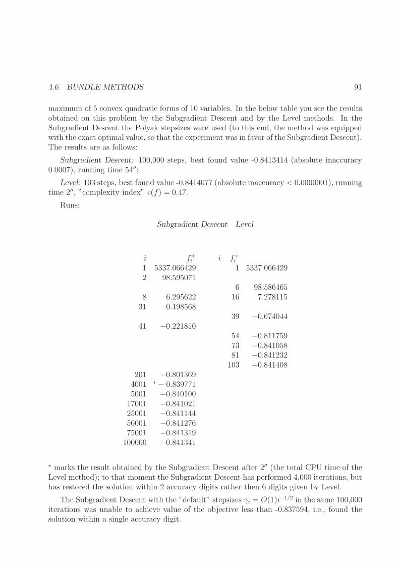
maximum of 5 convex quadratic forms of 10 variables. In the below table you see the resultsobtained on this problem by the Subgradient Descent and by the Level methods. In theSubgradient Descent the Polyak stepsizes were used (to this end, the method was equippedwith the exact optimal value, so that the experiment was in favor of the Subgradient Descent).The results are as follows:

Subgradient Descent: 100,000 steps, best found value -0.8413414 (absolute inaccuracy0.0007), running time 54′′;

Level: 103 steps, best found value -0.8414077 (absolute inaccuracy < 0.0000001), runningtime 2′′, ”complexity index” c(f) = 0.47.

Runs:

Subgradient Descent Level

i f+i i f+

i

1 5337.066429 1 5337.0664292 98.595071

6 98.5864658 6.295622 16 7.27811531 0.198568

39 −0.67404441 −0.221810

54 −0.81175973 −0.84105881 −0.841232103 −0.841408

201 −0.8013694001 ∗ − 0.8397715001 −0.84010017001 −0.84102125001 −0.84114450001 −0.84127675001 −0.841319100000 −0.841341

∗ marks the result obtained by the Subgradient Descent after 2′′ (the total CPU time of theLevel method); to that moment the Subgradient Descent has performed 4,000 iterations, buthas restored the solution within 2 accuracy digits rather then 6 digits given by Level.

The Subgradient Descent with the ”default” stepsizes γi = O(1)i−1/2 in the same 100,000iterations was unable to achieve value of the objective less than -0.837594, i.e., found thesolution within a single accuracy digit.


4.7 Exercises

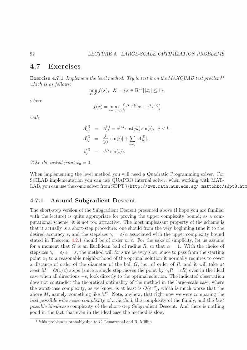
Exercise 4.7.1 Implement the level method. Try to test it on the MAXQUAD test problem1)

which is as follows:minx∈X

f(x), X = x ∈ R10| |xi| ≤ 1,

wheref(x) = max

i=1,...,5

(xTA(i)x+ xT b(i)

)

with

A(i)kj = A

(i)jk = ej/k cos(jk) sin(i), j < k;

A(i)jj =

j

10| sin(i)|+

∑

k 6=j

|A(i)jk |,

b(i)j = ej/i sin(ij).

Take the initial point x0 = 0.

When implementing the level method you will need a Quadratic Programming solver. ForSCILAB implementation you can use QUAPRO internal solver, when working with MAT-LAB, you can use the conic solver from SDPT3 (http://www.math.nus.edu.sg/ mattohkc/sdpt3.html

4.7.1 Around Subgradient Descent

The short-step version of the Subgradient Descent presented above (I hope you are familiarwith the lecture) is quite appropriate for proving the upper complexity bound; as a com-putational scheme, it is not too attractive. The most unpleasant property of the scheme isthat it actually is a short-step procedure: one should from the very beginning tune it to thedesired accuracy ε, and the stepsizes γi = ε/α associated with the upper complexity boundstated in Theorem 4.2.1 should be of order of ε. For the sake of simplicity, let us assumefor a moment that G is an Euclidean ball of radius R, so that α = 1. With the choice ofstepsizes γi = ε/α = ε, the method will for sure be very slow, since to pass from the startingpoint x1 to a reasonable neighborhood of the optimal solution it normally requires to covera distance of order of the diameter of the ball G, i.e., of order of R, and it will take atleast M = O(1/ε) steps (since a single step moves the point by γiR = εR) even in the idealcase when all directions −ei look directly to the optimal solution. The indicated observationdoes not contradict the theoretical optimality of the method in the large-scale case, wherethe worst-case complexity, as we know, is at least is O(ε−2), which is much worse that theabove M , namely, something like M2. Note, anyhow, that right now we were comparing thebest possible worst-case complexity of a method, the complexity of the family, and the bestpossible ideal-case complexity of the short-step Subgradient Descent. And there is nothinggood in the fact that even in the ideal case the method is slow.

1 )this problem is probably due to C. Lemarechal and R. Mifflin

4.7. EXERCISES 93

There are, anyhow, more or less evident possibilities to make the method computationallymore reasonable. The idea is not to tune the method to the prescribed accuracy in advance,thus making the stepsizes small from the very beginning, but to start with ”large” stepsizesand then decrease them at a reasonable rate. To implement the idea, we need an auxiliarytool (which is important an interesting in its own right), namely, projections.

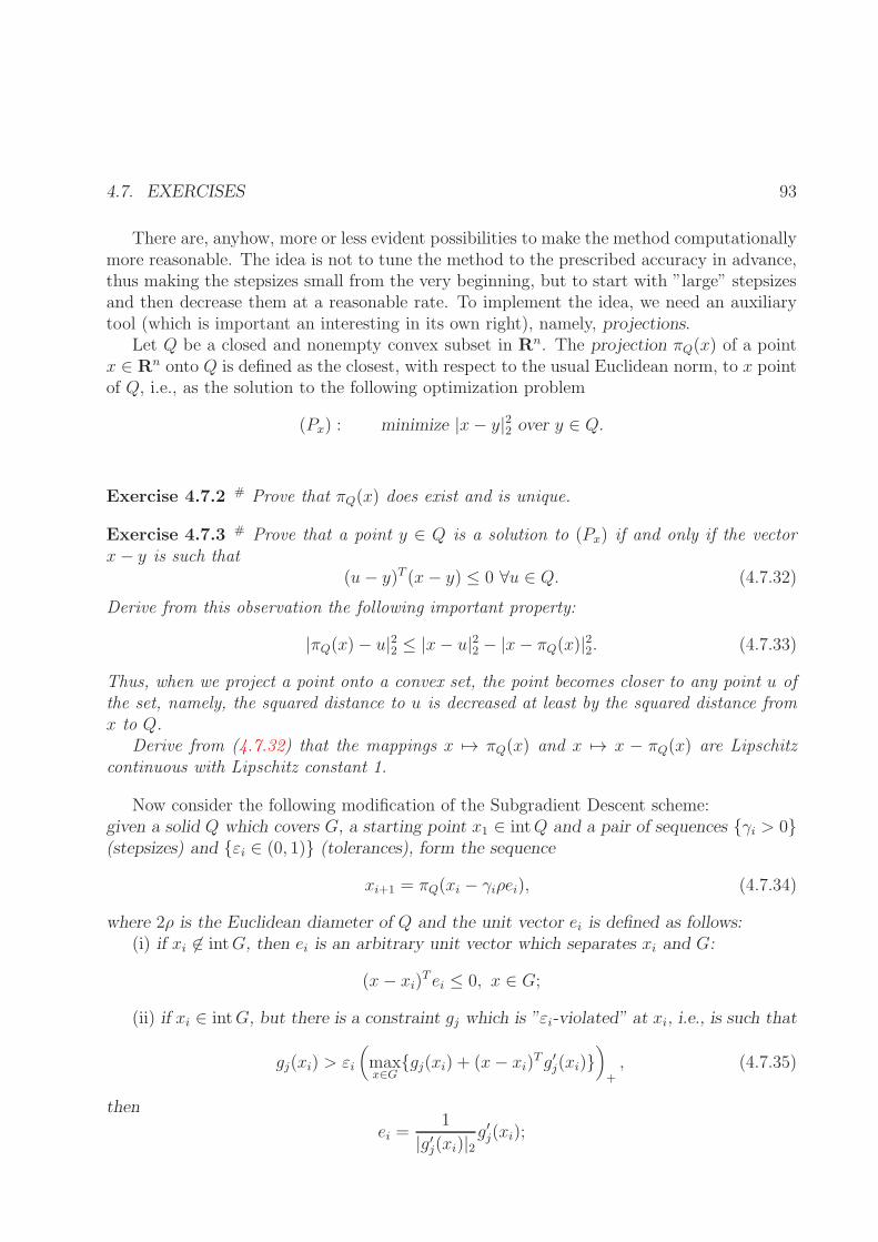
Let Q be a closed and nonempty convex subset in Rn. The projection πQ(x) of a pointx ∈ Rn onto Q is defined as the closest, with respect to the usual Euclidean norm, to x pointof Q, i.e., as the solution to the following optimization problem

(Px) : minimize |x− y|22 over y ∈ Q.

Exercise 4.7.2 # Prove that πQ(x) does exist and is unique.

Exercise 4.7.3 # Prove that a point y ∈ Q is a solution to (Px) if and only if the vectorx− y is such that

(u− y)T (x− y) ≤ 0 ∀u ∈ Q. (4.7.32)

Derive from this observation the following important property:

|πQ(x)− u|22 ≤ |x− u|22 − |x− πQ(x)|22. (4.7.33)

Thus, when we project a point onto a convex set, the point becomes closer to any point u ofthe set, namely, the squared distance to u is decreased at least by the squared distance fromx to Q.

Derive from (4.7.32) that the mappings x 7→ πQ(x) and x 7→ x − πQ(x) are Lipschitzcontinuous with Lipschitz constant 1.

Now consider the following modification of the Subgradient Descent scheme:given a solid Q which covers G, a starting point x1 ∈ intQ and a pair of sequences γi > 0(stepsizes) and εi ∈ (0, 1) (tolerances), form the sequence

xi+1 = πQ(xi − γiρei), (4.7.34)

where 2ρ is the Euclidean diameter of Q and the unit vector ei is defined as follows:(i) if xi 6∈ intG, then ei is an arbitrary unit vector which separates xi and G:

(x− xi)T ei ≤ 0, x ∈ G;

(ii) if xi ∈ intG, but there is a constraint gj which is ”εi-violated” at xi, i.e., is such that

gj(xi) > εi

(maxx∈G

gj(xi) + (x− xi)Tg′j(xi)

)

+, (4.7.35)

then

ei =1

|g′j(xi)|2g′j(xi);


(iii) if xi ∈ intG and no constraint is εi-violated at xi, i.e., no inequality (4.7.35) issatisfied, then

ei =1

|f ′(xi)|2f ′(xi).

If in the case of (iii) f ′(xi) = 0, then ei is an arbitrary unit vector.After ei is chosen, loop.The modification, as we see, is in the following:1) We add projection onto a covering G solid Q into the rule defining the updating

xi 7→ xi+1 and use the half of the diameter of Q as the scale factor in the steplength (in thebasic version of the method, there was no projection, and the scale factor was the radius ofthe ball Vout);

2) We use time-dependent tactics to distinguish between search points which ”almostsatisfy” the functional constraints and those which ”significantly violate” a constraint.

3) If we meet with a productive point xi with vanishing subgradient of the objective,we choose as ei an arbitrary unit vector and continue the process. Note that in the initialversion of the method in the case in question we terminate and claim that xi is an ε-solution;now we also could terminate and claim that xi is an εi-solution, which in fact is the case,but εi could be large, not the accuracy we actually are interested in.

Exercise 4.7.4 # Prove the following modification of Proposition 4.3.1:Let a problem (p) from the family Pm(G) be solved by the aforementioned Subgradient

Descent method with nonincreasing sequence of tolerances εi. Assume that for a pair ofpositive integers N > N ′ one has

Γ(N ′ : N) ≡ 2 + 12

∑Nj=N ′ γ2j∑N

j=N ′ γj< εN

rinρ, (4.7.36)

where rin is the maximal of radii of Euclidean balls contained in G. Then among the searchpoints xN ′ , xN ′+1, ..., xN there were productive ones, and the best of them (i.e., that one withthe smallest value of the objective) point xN ′,N is an εN ′-solution to (p).

Derive from this result that in the case of problems without functional constraints (m = 0),where εi do not influence the process at all, the relation

ε∗(N) ≡ minN≥M≥M ′≥1

ρΓ(M ′ :M)/rin < 1 (4.7.37)

implies that the best of the productive search points found in course of the first N steps iswell-defined and is an ε∗(N)-solution to (p).

Hint: follow the line of argument of the original proof of Proposition 4.3.1. Namely, apply theproof to the ”shifted” process which starts at xN ′ and uses at its i-th iteration, i ≥ 1, the stepsizeγi+N ′−1 and the tolerance εi+N ′−1. This process differs from that one considered in the lecture intwo issues:

(1) presence of time-varying tolerance in detecting productivity and an ”arbitrary” step, insteadof termination, when a productive search point with vanishing subgradient of the objective is met;

4.7. EXERCISES 95

(2) exploiting the projection onto Q ⊃ G when updating the search points.To handle (1), prove the following version of Proposition 3.3.1 (Lecture 3):Assume that we are generating a sequence of search points xi ∈ Rn and associate with these

points vectors ei and approximate solutions xi in accordance to (i)-(iii). Let

Gi = x ∈ G | (x− xj)T ej ≤ 0, 1 ≤ j ≤ i,

and let Size be a size. Assume that for some M

Size(GM ) < εM Size(G)

(if GM is not a solid, then, by definition, Size(GM ) = 0). Then among the search points x1, ..., xMthere were productive ones, and the best (with the smallest value of the objective) of these pro-ductive points is a ε1-solution to the problem.

To handle (2), note that when estimating InnerRad(GN ), we used the equalities

|xj+1 − x+|22 = |xj − x+|22 + ...

and would be quite satisfied if = in these inequalities would be replaced with ≤; in view of Exercise

4.7.3, this replacement is exactly what the projection does.

Looking at the statement given by Exercise 4.7.4, we may ask ourselves what could be areasonable way to choose the stepsizes γi and the tolerances εi. Let us start with the caseof problems without functional constraints, where we can forget about the tolerances - theydo not influence the process. What we are interested in is to minimize over stepsizes thequantities ε∗(N). For a given pair of positive integers M ≥M ′ the minimum of the quantity

Γ(N ′ : N) =2 + 1

2

∑Mj=M ′ γ2j∑M

j=M ′ γj

over positive γj is attained when γj = 2√M−M ′+1

, M ′ ≤ j ≤ M , and is equal to 2√M−M ′+1

;

thus, to minimize ε∗(N) for a given i, one should set γj = 2√N, j = 1, ..., N , which would

result inε∗(N) = 2N−1/2 ρ

rin.

This is, basically, the choice of stepsizes we used in the short-step version of the SubgradientDescent; an unpleasant property of this choice is that it is ”tied” to N , and we would liketo avoid necessity to fix in advance the number of steps allowed for the method. A naturalidea is to use the recommendation γj = 2N−1/2 in the ”sliding” way, i.e., to set

γj = 2j−1/2, j = 1, 2, ... (4.7.38)

Let us look what will be the quantities ε∗(N) for the stepsizes (4.7.38).

Exercise 4.7.5 # Prove that for the stepsizes (4.7.38) one has

ε∗(N) ≤ Γ(]N/2[: N)ρ

rin≤ κN−1/2 ρ

rin

with certain absolute constant κ. Compute the constant.


We see that the stepsizes (4.7.38) result in optimal, up to an absolute constant factor, rate ofconvergence of the quantities ε∗(N) to 0 as N → ∞. Thus, when solving problems withoutfunctional constraints, it is reasonable to use the aforementioned Subgradient Descent withstepsizes (4.7.38); according to the second statement of Exercise 4.7.4 and Exercise 4.7.5, forall N such that

ε(N) ≡ κN−1/2 ρ

rin< 1

the best of the productive search points found in course of the first N steps is well-definedand solves the problem within relative accuracy ε(N).

Now let us look at problems with functional constraints. It is natural to use here thesame rule (4.7.38); the only question now is how to choose the tolerances εi. A reasonablepolicy would be something like

εi = min0.9999, 1.01κi−1/2 ρ

rin, (4.7.39)

Exercise 4.7.6 # Prove that the Subgradient Descent with stepsizes (4.7.38) and tolerances(4.7.39), as applied to a problem (p) from the family Pm(G), possesses the following conver-gence properties: for all N such that

κN−1/2 ρ

rin< 0.99

among the search points x]N/2[, x]N/2[+1, ..., xN there are productive ones, and the best (withthe smallest value of the objective) of these points solves (p) within relative inaccuracy notexceeding

ε]N/2[ ≤ χN−1/2 ρ

rin,

χ being an absolute constant.Note that if one chooses Q = Vout (i.e., ρ = R, so that ρ/rini = α is the asphericity of

G), then the indicated rate of convergence results in the same (up to an absolute constantfactor) as for the basic short-step Subgradient Descent complexity of solving problems fromthe family within relative accuracy ε.

4.7.2 Mirror Descent

Looking at the 3-line convergence proof for the standard Subgradient Descent:

xi+1 = πG(xi−γif ′(xi)/|f ′(xi)|) ⇒ |xi+1−x∗|2 ≤ |xi−x∗|2−2γi(xi−x∗)Tf ′(xi)/|f ′(xi)|+γ2i

⇒ |xi+1 − x∗|2 ≤ |xi − x∗|2 − 2γi(f(xi)− f ∗)/|f ′(xi)|+ γ2i

⇒ mini≤N

f(xi)− f ∗ ≤ |x1 − x∗|2 +∑Ni=1 γ

2i

2∑N

i=1 γi

4.7. EXERCISES 97

one should be surprised. Indeed, all of us know the origin of the gradient descent: if f issmooth, a step in the antigradient direction decreases the first-order expansion of f andtherefore, for a reasonably chosen stepsize, increases f itself. Note that this standard rea-soning has nothing in common with the above one: we deal with a nonsmooth f , and itshould not decrease in the direction of an anti-subgradient independently of how small is thestepsize; there is a subgradient in the subgradient set which actually possesses the desiredproperty, but this is not necessarily the subgradient used in the method, and even with the”good” subgradient you could say nothing about the amount the objective can be decreasedby. The ”correct” reasoning deals with algebraic structure of the Euclidean norm ratherthan with local behavior of the objective, which is very surprising; it is a kind of miracle.But we are interested in understanding, not in miracles. Let us try to understand what isbehind the phenomenon we have met.

First of all, what is a subgradient? Is it actually a vector? The answer, of course, is ”no”.Given a convex function f defined on an n-dimensional vector space E and an interior pointx of the domain of f , you can define a nonempty set of support functionals - linear formsf ′(x)[h] of h ∈ E which are support to f at x, i.e., such that

f(y) ≥ f(x) + f ′(x)[y − x], y ∈ Dom f ;

these forms are intrinsically associated with f and x. Now, having chosen somehow anEuclidean structure (·, ·) on E, you may associate with linear forms f ′(x)[h] vectors f ′(x)from E in such a way that

f ′(x)[h] = (f ′(x), h), h ∈ Rn,

thus coming from support functionals to subgradients-vectors. The crucial point is thatthese vectors are not defined by f and x only; they also depend on what is the Euclideanstructure on E we use. Of course, normally we think of an n-dimensional space as of thecoordinate space Rn with once for ever fixed Euclidean structure, but this habit sometimesis dangerous; the problems we are interested in are defined in affine terms, not in the metricones, so why should we always look at the problems via certain once for ever fixed Euclideanstructure which has nothing in common with the problem? Developing systematically thisevident observation, one may come to the most advanced and recent convex optimizationmethods like the polynomial time interior point ones. Our goal now is much more modest,but we also shall get profit from the aforementioned observation. Thus, once more: the”correct” objects associated with f and x are not vectors from E, but elements of the dualto E space E∗ of linear forms on E. Of course, E∗ is of the same dimension as E andtherefore it can be identified with E; but there are many ways to identify these spaces, andno one of them is ”natural”, more preferable than others.

Since the support functionals f ′(x)[h] ”live” in the dual space, the Gradient Descentcannot avoid the necessity to identify somehow the initial - primal - and the dual space, andthis is done via the Euclidean structure the method is related to - as it was already explained,this is what allows to associate with a support functional - something which ”actually exists”,but belongs to the dual space - a subgradient, a vector belonging to the primal space; in


a sense, this vector is a phantom - it depends on the Euclidean structure on E. Now, isa Euclidean structure the only way to identify the dual and the primal spaces? Of course,no, there are many other ways. What we are about to do is to consider certain family of”identifications” of E and E∗ which includes, as particular cases, all identifications given byEuclidean structures. This family is as follows. Let V (φ) be a smooth (say, continuouslydifferentiable) convex function on E∗; its support functional V ′(φ)[·] at a point φ is a linearfunctional on the dual space. Due to the well-known fact of Linear Algebra, every linearform L[η] on the dual space is defined by a vector l from the primal space, in the sense that

L[η] = η[l]

for all η ∈ E∗; this vector is uniquely defined, and the mapping L 7→ l is a linear isomorphismbetween the space (E∗)∗ dual to E∗ and the primal space E. This isomorphism is ”canonical”- it does not depend on any additional structures on the spaces in question, like innerproducts, coordinates, etc., it is given by intrinsic nature of the spaces. In other words, inthe quantity φ[x] we may think of φ being fixed and x varying over E, which gives us alinear form on E (this is the origin of the quantity); but we also can think of x as being fixedand φ varying over E∗, which gives us a linear form on E∗; and Linear Algebra says to usthat every linear form on E∗ can be obtained in this manner from certain uniquely definedx ∈ E. Bearing in mind this symmetry, let us from now on renotate the quantity φ[x] as〈φ, x〉, thus using more ”symmetric” notation.

Thus, every linear form on E∗ corresponds to certain x ∈ E; in particular, the linearform V ′(φ)[·] on E∗ corresponds to certain vector V ′(φ) ∈ E:

V ′(φ)[η] ≡ 〈η, V ′(φ)〉 , η ∈ E∗.

We come to certain mappingφ 7→ V ′(φ) : E∗ → E;

this mapping, under some mild assumptions, is a continuous one-to-one mapping with con-tinuous inverse, i.e., is certain identification (not necessarily linear) of the dual and theprimal spaces.

Exercise 4.7.7 Let (·, ·) be certain Euclidean structure on the dual space, and let

V (φ) =1

2(φ, φ).

The aforementioned construction associates with V the mapping φ 7→ V ′(φ) : E → E∗; onthe other hand, the Euclidean structure in question itself defines certain identification of thedual and the primal space, the identification I given by the identity

φ[x] = (φ, I−1x), φ ∈ E∗, x ∈ E.

Prove that I = V ′.Assume that eini=1 is a basis in E and e∗i is the biorthonormal basis in E∗ (so that

e∗i [ej] = δij), and let A be the matrix which represents the inner product in the coordinatesof E∗ related to the basis e∗i , i.e., Aij = (e∗i , e

∗j ). What is the matrix of the associated

mapping V ′ taken with respect to the e∗i -coordinates in E∗ and the ei-coordinates in E?

4.7. EXERCISES 99

We see that all ”standard” identifications of the primal and the dual spaces, i.e., those givenby Euclidean structures, are covered by our mappings φ 7→ V ′(φ); the corresponding V ’s are,up to the factor 1/2, squared Euclidean norms. A natural question is what are the mappingsassociated with other squared norms.

Exercise 4.7.8 Let ‖ · ‖ be a norm on E, let

‖φ‖∗ = maxφ[x] | x ∈ E, ‖x‖ ≤ 1

be the conjugate norm on and assume that the function

V‖·‖∗(φ) =1

2‖φ‖2∗

is continuously differentiable. Then the mapping φ 7→ V ′(φ) is as follows: you take a linearform φ 6= 0 on E, maximize it on the ‖ · ‖-unit ball of E; the maximizer is unique and isexactly V ′(φ); and, of course, V ′(0) = 0. In other words, V ′(φ) is nothing but the ”directionof the fastest growth” of the functional φ, where, of course, the rate of growth in a directionis defined as the ”progress in φ per ‖ · ‖-unit step in the direction”.

Prove that the mapping φ 7→ φ′ is a continuous mapping form E onto E ′. Prove thatthis mapping is a continuous one-to-one correspondence between E and E ′ if and only if thefunction

W‖·‖(x) =1

2‖x‖2 : E → R

is continuously differentiable, and in this case the mapping

x 7→W ′‖·‖(x)

is nothing but the inverse to the mapping given by V ′‖·‖∗.

Now, every Euclidean norm ‖ · ‖ on E induces, as we know, a Subgradient Descent methodfor minimization of convex functions over closed convex domains in E. Let us write downthis method in terms of the corresponding function V‖·‖∗ . For the sake of simplicity let usignore for the moment the projector πG, thus looking at the method for minimizing over thewhole E. The method, as it is easily seen, would become

φi+1 = φi − γif′(xi)/‖f ′(xi)‖∗, xi = V ′(φi), V ≡ V‖·‖∗ . (4.7.40)

Now, in the presented form of the Subgradient Descent there is nothing from the fact that‖ · ‖ is a Euclidean norm; the only property of the norm which we actually need is thedifferentiability of the associated function V . Thus, given a norm ‖ · ‖ on E which inducesa differentiable outside 0 conjugate norm on the conjugate space, we can write down certainmethod for minimizing convex functions over E. How could we analyze the convergenceproperties of the method? In the case of the usual Subgradient Descent the proof of con-vergence was based on the fact that the anti-gradient direction f ′(x) is a descent direction


for certain Lyapunov function, namely, |x − x∗|2, x∗ being a minimizer of f . In fact ourreasoning was as follows: since f is convex, we have

〈f ′(x), x∗ − x〉 ≤ f(x)− f(x∗) ≤ 0, (4.7.41)

and the quantity 〈f ′(x), x− x∗〉 is, up to the constant factor 2, the derivative of the function|x− x∗|2 in the direction f ′(x). Could we say something similar in the general case, where,according to (4.7.40), we should deal with the situation x = V ′(φ)? With this substitution,the left hand side of (4.7.41) becomes

〈f ′(x), x∗ − V ′(φ)〉 = d

dt|t=0 V

+(φ− tf ′(x)), V +(ψ) = V (ψ)− 〈ψ, x∗〉 .

Thus, we can associate with (4.7.40) the function

V +(φ) ≡ V +‖·‖∗(φ) = V‖·‖∗(φ)− 〈φ, x∗〉 , (4.7.42)

x∗ being a minimizer of f , and the derivative of this function in the direction −f ′(V ′(φ)) ofthe trajectory (4.7.40) is nonpositive:

⟨−f ′(V ′(φ)), (V +)′(φ)

⟩≤ f(x∗)− f(x) ≤ 0, φ ∈ E∗. (4.7.43)

Now we may try to reproduce the reasoning which leads to the rate-of-convergence estimatefor the Subgradient Descent for our now situation, where we speak about process (4.7.40)associated with an arbitrary norm on E (the norm should result, of course, in a continuouslydifferentiable V ).

For the sake of simplicity, let us restrict ourselves with the simple case when V possessesa Lipschitz continuous derivative. Thus, from now on let ‖ · ‖ be a norm on E such that themapping

V(φ) ≡ V ′‖·‖∗(φ) : E

∗ → E

is Lipschitz continuous, and let

L ≡ L‖·‖ = sup‖V(φ′)− V(φ′′)‖

‖φ′ − φ′′‖∗| φ′ 6= φ′′, φ′, φ′′ ∈ E∗.

For the sake of brevity, from now on we write V instead of V‖·‖∗ .

Exercise 4.7.9 Prove that

V (φ+ η) ≤ V (φ) + 〈η,V(φ)〉+ LV (η), φ, η ∈ E∗. (4.7.44)

Now let us investigate process (4.7.40).

Exercise 4.7.10 ∗ Let f : E → R be a Lipschitz continuous convex function which attainsits minimum on E at certain point x∗. Consider process (cf. (4.7.40))

φi+1 = φi − γif′(xi)/|f ′(xi)|∗, xi = V ′(φi), φ1 = 0, (4.7.45)

4.7. EXERCISES 101

and let xi be the best (with the smallest value of f) of the points x1, ..., xi and let εi =f(xi)−minE f . Prove that then

εN ≤ L‖·‖(f)|x∗|2 + L∑N

i=1 γ2i

2∑N

i=1 γi, N = 1, 2, ... (4.7.46)

where L‖·‖(f) is the Lipschitz constant of f with respect to the norm ‖ · ‖. In particular, themethod converges, provided that

∑

i

γi = ∞, γi → 0, i→ ∞.

Hint: use the result of exercise 4.7.9 and (4.7.43) to demonstrate that

V +(φi+1) ≤ V +(φi)− 2γi(f(xi)− f ∗)/|f ′(xi)|∗ +L2γ2i , V

+(φ) = V (φ)− 〈φ, x∗〉 ,

and then act exactly as in the case of the usual Subgradient Descent. Note that the basicresult explains what is the origin of the ”Subgradient Descent miracle” which motivated ourconsiderations; as we see, this miracle comes not from the very specific algebraic structure ofthe Euclidean norm, but from certain ”robust” analytic property of the norm (the Lipschitzcontinuity of the derivative of the conjugate norm), and we can fabricate similar miraclesfor arbitrary norms which share the indicated property. In fact you could use the outlinedMirror Descent scheme, developed by Nemirovski and Yudin, with necessary (and more orless straightforward) modifications, in order to extend everything what we know about theusual - ”Euclidean” - Subgradient Descent (I mean, the versions for optimization over adomain rather than over the whole space and for optimization over solids under functionalconstraints) onto the general ”non-Euclidean” case, but we skip here these issues.

4.7.3 Stochastic Approximation

We shall speak here about a problem which is quite different from those considered sofar – about stochastic optimization. The simplest (and, perhaps, the most important inapplications) single-stage Stochastic Programming program is as follows:

minimize f(x) =∫

ΩF (x, ω)dP (ω) s.t. x ∈ G. (4.7.47)

Here

• F (x, ω) are functions of the design vector x ∈ Rn and parameter w ∈ Ω

• G is a subset in Rn

• P is a probability distribution on the set Ω.


Thus, a stochastic program is a Mathematical Programming program where the objectiveand the constraints are expectations of certain functions depending both of the design vectorx and random parameter ω.

The main source of programs of the indicated type is optimization in stochastic systems,like Queing Networks, where the processes depend not only on the design parameters, likeperformances and numbers of serving devices of different types), but also on random factors.As a result, the characteristics of such a system (e.g., time of serving a client, cost of service,etc.) are random variables depending, as on parameters, on the design parameters of thesystem. It is reasonable to measure the quality of the system by the expected values of theindicated random variables (in the dynamic systems, we should speak about the steady-stateexpectations). These expected values have the form of the objective and the constraints in(4.7.47), so that to optimize a system in question over its design parameters is a program ofthe type (4.7.47).

Looking at stochastic program (4.7.47), you can immediately ask what are, if any, thespecific features of these problems and why these problems need specific treatment. (4.7.47)is, finally, nothing but the usual Mathematical Programming problem; we know how to solvetractable (convex) Mathematical Programming programs, and to the moment we never tookinto account what is the origin of the objective and the constraints, are they given by explicitsimple formulae, or are they intergals, as in (4.7.47), or solutions to differential equations,or whatever else. All what was important for us were the properties of the objective and theconstraints – convexity, smoothness, etc., but not their origin.

This “indifference to the origin of the problem” indeed was the feature of our approach,but it was its weak point, not the strong one. In actual computations, the performanceof an algorithm heavily depends not only on the quality of the method we apply to solvethe problem, but also on the computational effort needed to provide the algorithm by theinformation on the problem instance – the job which in our model of optimization was thetask of the oracle. We did not think how to help the oracle to solve his task and took careonly of total number of oracle calls – we did our best to reduce this number. In the mostgeneral case, when we have no idea of what is the internal structure of the problem, this isthe only possible approach. But the more we know about the structure of the problem, themore should we think of how to simplify the task of the oracle in order to reduce the overallcomputational expenses.

Stochastic Programming is an example when we know something about the structure ofthe problem in question. Namely, let us look at a typical stochastic system, like QueingNetwork. Normally the function F (x, ω) associated with the system is “algorithmicallysimple” – given x and ω, we can more or less easily compute the quantity F (x, ω) andeven its derivative with respect to x; to this end it suffices to create a simulation model ofthe system and run it at the given by ω realization of the random parameters (arrival andservice times, etc.); even for a rather sophisticated system, a single simulation of this typeis relatively fast. Thus, typically we have no difficulties with simulating realizations of therandom quantity F (x, ·). On the other hand, even for relatively simple systems it is, asa rule, impossible to compute the expected values of the indicated quantities in a “closedanalytic form”, and the only way to evaluate these expected values if to use a kind of the

4.7. EXERCISES 103

Monte-Carlo method: to run not a single, but many simulations, for a fixed value of thedesign parameters, and to take the empiric average of the observed random quantities asan estimate of their expected values. According to the well-known results on the rate ofconvergence of the Monte-Carlo method, to estimate the expected values within inaccuracyǫ it requires O(1/ǫ2) simulations, and this is just to get the estimate of the objective and theconstraints of problem (4.7.47) at a single point! Now imagine that we are going to treat(4.7.47) as a usual “black-box represented” optimization problem and intend to imitate theusual first-order oracle for it via the afrementioned Monte-Carlo estimator. In order to getan ǫ-solution to the problem, we, even in good cases, need to estimate within accuracy O(ǫ)the objective and the constraints along the search points. It means that the method willrequire much more simulations than the aforementioned O(1/ǫ2): this quantity should bemultiplied by the information-based complexity of the optimization method we are going touse. As a result, the indicated approach in most of the cases results in unappropriately longcomputations.

An extremely surprising thing is that there exists another way to solve the problem.This way, under reasonable convexity assumptions, results in overall number of O(1/ǫ2)computations only – as if there were no optimization at all and the only goal were to estimatethe objective and the constraints at a given point. The subject of our today lecture is thisother way – Stochastic Approximation.

To get a convenient framework for presenting Stochastic Approximation, it is worthy tomodify a little the way we are looking at our problem. Assume that when solving it, weare allowed to generate a random sample ω1, ω2,... of “random factors” involved into theproblem; the elements of the sample are assumed to be mutually independent and distributedaccording to P . Assume also that given x and ω, we are able to compute the value F (x, ω)and the gradient ∇xF (x, ω) of the integrant in (4.7.47). Note that under mild regularityassumptions the differentiation with respect to x and taking expectation are interchangeable:

f(x) =∫

ΩF (x, ω)dP (ω), ∇f(x) =

∫

Ω∇xF (x, ω)dP (ω). (4.7.48)

It means that the situation is covered by the following model of an optimization methodsolving (4.7.47):

At a step i, we (the method) form i-th search point xi and forward it to the oracle whichwe have in our disposal. The oracle returns the quantities

F (xi, ωi), ∇xF (xi, ωi)

(in our previous interpretation it means that a single simulation of the stochastic systemin question is performed), and this answer is the portion of information on the problem weget on the step in question. Using the information accumulated so far, we generate the newsearch point xi+1, again forward it to the oracle, enrich our accumulated information by itsanswer, and so on.

The presented scheme is a very natural definition of a method based on stochastic firstorder oracle capable to provide the method with random unbiased (see (4.7.48)) estimates of


the values and the gradients of the objective and the constraints of (4.7.47). Note that theestimates are not only unbiased, but also form a kind of Markov chain: the distribution ofthe answers of the oracle at a point depends only on the point, not on the previous answers(recall that ωi are assumed to be independent).

Now, for our further considerations it is completely unimportant that the observationof f(x) comes from the value, and the observation of ∇f(x) comes from the gradient. Itsuffices to postulate the following:

• The goal is to solve the Convex Programming program2

f0(x) → min, | x ∈ G ⊂ Rn (4.7.49)

[G is closed and convex, f is convex and Lipschitz continuous on G]

• The information obtained by an optimization method at i-th step, i = 1, 2, ..., comesfrom a stochastic oracle, i.e., is a real and a vector

φ(xi, ωi) ∈ R, ψ(xi, ωi) ∈ Rn,

where

– ωi is sequence of independent identically distributed, according to certain prob-ability distribution P , random parameters taking values in certain space Ω;

– xi is i-th search point generated by the method; this point may be an arbitrarydeterministic function of the information obtained by the method so far (i.e., atthe steps 1, ..., i− 1)

It is assumed (and it is crucial) that the information obtained by the method is unbi-ased:

Eφ(x, ω) = f(x), f ′(x) ≡ Eψ(x, ω) ∈ ∂f(x), x ∈ G; (4.7.50)

here E is the expectation with respect to the distribution of the random parameters inquestion.

To get reasonable complexity results, we need to bound somehow the magnitude of therandom noise in the process in the stochastic oracle (as it is always done in all statisticalconsiderations). Mathematically, the most convenient way to do it is as follows: let

L = supx∈G

E|ψ(x, f)|2

1/2. (4.7.51)

From now on we assume that the oracle is such that L < ∞. The quantity L will becalled the intensity of the oracle at the problem in question; in what follows it plays thesame role as the Lipschitz constant of the objective in large-scale minimization of Lipschitzcontinuous convex functions.

2Of course, the model we are about to present makes sense not only for convex programs; but the methodswe are interested in will, as always, work well only in convex case, so that we loose nothing when imposingthe convexity assumption from the very beginning

4.7. EXERCISES 105

4.7.4 The Stochastic Approximation method

The method we are interested in is completely similar to the Subgradient Descent methodfrom Section 4.5. Namely, the method generates search points according to the recurrency(cf. (8.1.1))

xi+1 = πG(xi − γiψ(xi, ωi)), i = 1, 2, ..., (4.7.52)

where

• x1 ∈ G is an arbitrary starting point;

• γi are deterministic positive stepsizes;

• πG(x) = argminy∈G |x− y| is the standard projector on G.

The only difference with (8.1.1) is that now we replace the direction g(xi) = f ′(xi)/|f ′(xi)|of the subgradinet of f at xi by the random estimate ψ(xi, ωi) of the subgradient.

Note that the search trajectory of the method is governed by the random variables ωi

and is therefore random:xi = xi(ω

i−1), ωs = (ω1, ..., ωs).

Recurrency (4.7.52) defines the sequence of the search points, not that one of the approx-imate solutions. In the deterministic case of Section 4.5 we extracted from the search pointsthe approximate solutions by choosing the best (with the smallest value of the objective) ofthe search points generated so far. The same could work in the stochastic case as well, buthere we meet with the following obstacle: we “do not see” the values of the objective, andtherefore cannot say which of the search point is better. To resolve the difficulty, we use thefollowing trick: define i-th approximate solution as the sliding average of the search points:

xi ≡ xi(ωi−1) =

∑

i/2≤t≤i

γi

−1

∑

i/2≤t≤i

γtxt. (4.7.53)

The efficiency of the resulting method is given by the following

Theorem 4.7.1 For the aforementined method one has, for all positive integer N ,

εN ≡ E [f(xN)−minx∈G

f(x)] ≤ D2 + L2∑N/2≤i≤N γ

2i

2∑

N/2≤i≤N γi, (4.7.54)

G being the diameter of G.In particular, for γi chosen accoding to

γi =D

L√i

(4.7.55)

one has

εN ≤ O(1)LD√N

(4.7.56)

with appropriately chosen absolute constant O(1).


Exercise 4.7.11 Prove Theorem 4.7.1.

Hint: follow the lines of the proof of the estimate (4.5.16) in Section 4.5; substitute d2i+1

with vi ≡ E|xi+1(ωi)− x∗|2.

Comments: The statement and the proof of Theorem 4.7.1 are completely similar to therelated “deterministic” considerations of Section 4.5. The only difference is that now we areestimating from above the expected inaccuracy of N -th approximate solution; this is quitenatural, since the stochastic nature of the process makes it impossible to say somethingreasonable about the quality of every realization of the random vector xN = xN (ωN−1)

It turns out that the rate of convergence established in (4.7.56) connot be improved.Namely, it is not difficult to prove the following statement.

Proposition 4.7.1 For every L > 0, any D > 0, any positive integer N and any stochastic-oracle-based N-step method M of minimizing univariate convex functions over the segmentG = [0, D] on the axis there exists a linear function f and a stochastic oracle with intensityL on the function such that

E [f(xN)−minGf ] ≥ O(1)

LD√N,

xN being the result formed by the method as applied to the problem f . Here O(1) is properlychosen positive absolute constant.

Note that in the deterministic case the rate of convergence O(1/√N) was unimprovable only

in the large-scale case; in contrast to this, in the stochastic case this rate becomes optimalalready when we are minimizing univariate linear functions.

Convergence rate O(1/√N) can be improved only if the objective is strongly convex. The

simplest and the most important result here is as follows (the proof is completely similar tothat one of Theorem 4.7.1):

Proposition 4.7.2 Assume that convex function f on Rn attains its minimum on G at aunique point x∗ and is such that

f(x∗) +θ

2|x− x∗|2 ≤ f(x) ≤ f(x∗) +

Θ

2|x− x∗|2, x ∈ G, (4.7.57)

with certain positive θ and Θ. Consider process (4.7.52) with the stepsizes

γi =γ

i, (4.7.58)

γ being a positive scale factor satisfying the relation

γθ > 1. (4.7.59)

4.7. EXERCISES 107

Then

εN ≡ E(f(xN)−minGf) ≤ c(γθ)Θ

D2 + γ2L2

N, (4.7.60)

where D is the diameter of G, L is the intensity of the oracle at the problem in question andc(·) is certain problem-independent function on (1,∞).

Exercise 4.7.12 Prove Proposition 4.7.2.

The algorithm (4.7.52) with the stepsizes (4.7.58) and the approximate solutions identical tothe search points is called the classical Stochastic Approximation; it originates from Kieferand Wolfovitz. A good news about the algorithm is its rate of convergence: O(1/N) insteadof O(1/

√N). A bad news is that this better rate is ensured only in the case of problems

satisfying (4.7.57) and that the rate of convergence is very sensitive to the choice of the scalefactor γ in the stepsize formula (4.7.58): if this scale factor does not satisfy (4.7.59), therate of convergence may become worse in order. To see this, consider the following simpleexample: the problem is

f(x) =1

2x2, [θ = Θ = 1]; G = [−1, 1]; x1 = 1,

the observations are given by

ψ(x, ω) = x+ ω [= f ′(x) + ω],

and ωi are the standard Gaussian random variables (Eωi = 0, Eω2i = 1); we do not specify

φ(x, ω), since it is not used in the algorithm. In this example, the best choice of γ is γ = 1 (inthis case one can make (4.7.59) an equality rather than strict inequality due to the extremesimplicity of the objective). For this choice of γ one has

Ef(xN+1) ≡ E [f(xN+1)−minxf(x)] ≤ 1

2N, N ≥ 1.

In particular, it takes no more than 50 steps to reach expected inaccuracy not exceeding0.01.

Now assume that when solving the problem we overestimate the quantity θ and choosestepsizes according to (4.7.58) with γ = 0.1. How many steps do we need in this case toreach the same expected inaccuracy 0.01 – 500, 5000, or what? The answer is astonishing:approximately 1,602,000 steps. And with γ = 0.05 (20 times less than the optimal value ofthe parameter) the same accuracy costs more than 5.2× 1014 steps!

We see how dangerous the “classical” rule (4.7.58) for the stepsizes is: underestimatingof γ (≡ overestimating of θ) may kill the procedure completely. And where from, in more orless complicated cases, could we take a reasonable estimate of θ? It should be said that thereexist stable versions of the classical Stochastic Approximation (they, same as our version ofthe routine, use “large”, as compared to O(1/i), stepsizes and take, as approximate solutions,certain averages of the search points). These stable version of the method are capable toreach (under assumptions similar to (4.7.57)) the O(1/N)-rate of convergence, even with


the “asymptotically optimal” coefficient at 1/N . Note, anyhow, that the nondegeneracyassumption (4.7.57) is crucial for the O(1/N)-rate of convergence; if it is removed, the bestpossible rate, as we know from Proposition 4.7.1, becomes O(1/

√N), and this is the rate

given by our “robust” Stochastic Approximation with “large” steps and averaging.

lecture 4 large-scale optimization...

Documents