lec 40ppts
DESCRIPTION
Turbo machineryTRANSCRIPT
1
Lect 40
2Prof. Bhaskar Roy, Prof. A M Pradeep, Department of Aerospace, IIT Bombay
Lect 40
Fundamentals of CFD for use in
Turbomachinery Analysis
3Prof. Bhaskar Roy, Prof. A M Pradeep, Department of Aerospace, IIT Bombay
Lect 40
• Physics of fluid mechanics are often captured in Partial Differential Equations (PDEs), mostly 2nd
order PDEs.
• Generally the governing equations are a set of coupled, non-linear PDEs valid within an arbitrary (or irregular) domain and are subject to various initial and boundary conditions.
• Purely analytical solutions of many fluid mechanic equations are limited due to imposition of various boundary conditions of typical fluid flow problems.
• Experimental data are often used for validation of CFD solutions. Together they are used for design purposes.
4Prof. Bhaskar Roy, Prof. A M Pradeep, Department of Aerospace, IIT Bombay
Lect 40
4
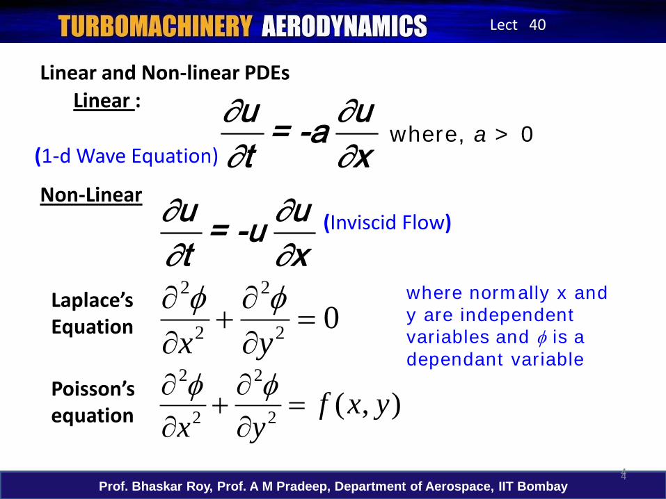
Linear and Non-linear PDEs
∂u ∂u= -a∂t ∂x
Linear :
(1-d Wave Equation)
∂u ∂u= -u∂t ∂x
Non-Linear(Inviscid Flow)
where, a > 0
02
2
2
2
=∂∂
+∂∂
yxφφ
),(2
2
2
2
yxfyx
=∂∂
+∂∂ φφ
Laplace’s Equation
Poisson’s equation
where normally x and y are independent variables and φ is a dependant variable
5Prof. Bhaskar Roy, Prof. A M Pradeep, Department of Aerospace, IIT Bombay
Lect 40
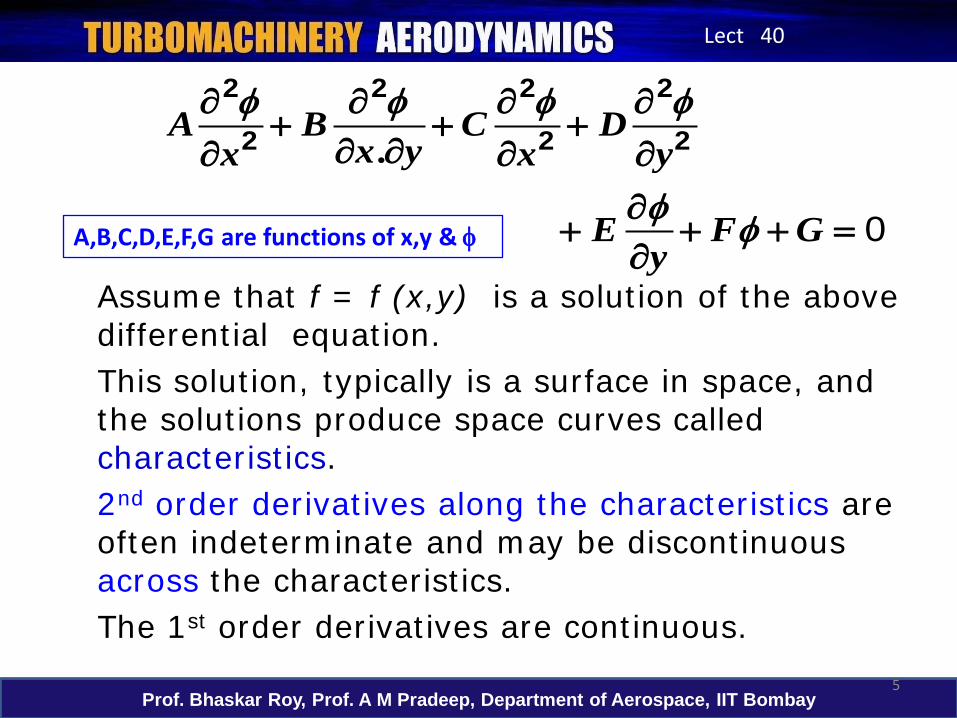
Assume that f = f (x,y) is a solution of the above differential equation.This solution, typically is a surface in space, and the solutions produce space curves called characteristics.2nd order derivatives along the characteristics are often indeterminate and may be discontinuous across the characteristics. The 1st order derivatives are continuous.
.
A B C Dx yx x y
E F Gy
φ φ φ φ
φ φ
∂ ∂ ∂ ∂+ + +
∂ ∂∂ ∂ ∂∂
+ + + =∂
2 2 2 2
2 2 2
0A,B,C,D,E,F,G are functions of x,y & φ
6Prof. Bhaskar Roy, Prof. A M Pradeep, Department of Aerospace, IIT Bombay
Lect 40
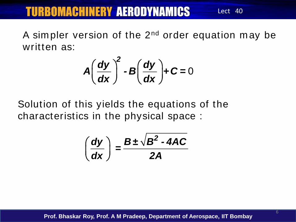
Solution of this yields the equations of the characteristics in the physical space :
02dy dyA - B +C =
dx dx
A simpler version of the 2nd order equation may be written as:
2dy B± B - 4AC=dx 2A
7Prof. Bhaskar Roy, Prof. A M Pradeep, Department of Aerospace, IIT Bombay
Lect 40
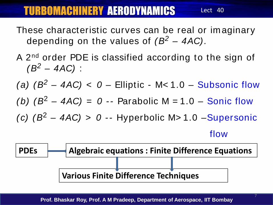
These characteristic curves can be real or imaginary depending on the values of (B2 – 4AC).
A 2nd order PDE is classified according to the sign of (B2 – 4AC) :
(a) (B2 – 4AC) < 0 – Elliptic - M<1.0 – Subsonic flow
(b) (B2 – 4AC) = 0 -- Parabolic M =1.0 – Sonic flow
(c) (B2 – 4AC) > 0 -- Hyperbolic M>1.0 –Supersonic
flow
Algebraic equations : Finite Difference Equations
Various Finite Difference Techniques
PDEs

8Prof. Bhaskar Roy, Prof. A M Pradeep, Department of Aerospace, IIT Bombay
Lect 40
• An Elliptic PDE has no real characteristics . A disturbance is propagated instantly in all directions within the region• The domain solution of an elliptic PDE is a closed region. Providing the boundary condition uniquely yields the solution within the domain• The solution domain for a parabolic PDE is open region. • For Parabolic PDE one characteristic line exists• A hyperbolic PDE has two characteristic lines• A complete description of 2nd order hyperbolic PDE requires two sets of initial conditions and two sets of boundary conditions

9Prof. Bhaskar Roy, Prof. A M Pradeep, Department of Aerospace, IIT Bombay
Lect 40
Initial and Boundary conditions (ICs and BCs)
ICs : A dependant variable is prescribed at some initial condn
BCs : A dependent variable or its derivative must satisfy on the boundary of the domain of the PDE
1) Dirichlet BC : Dependent Variable prescribed at boundary
2) Neumann BC: Normal gradient of the D.V. is specified
3) Robin BC : A linear combination of Dirichlet & Neumann
4) Mixed BC : Some part of the boundary has Dirichlet BC and some other part has Neumann BC
Body Surface Far Field Symmetry In / OutflowBCs
10Prof. Bhaskar Roy, Prof. A M Pradeep, Department of Aerospace, IIT Bombay
Lect 40
11 10
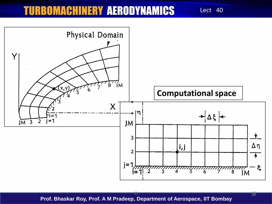
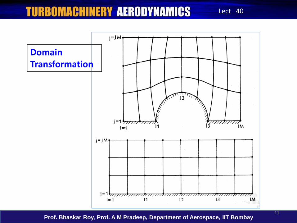
Computational space
11Prof. Bhaskar Roy, Prof. A M Pradeep, Department of Aerospace, IIT Bombay
Lect 40
Domain Transformation
12Prof. Bhaskar Roy, Prof. A M Pradeep, Department of Aerospace, IIT Bombay
Lect 40
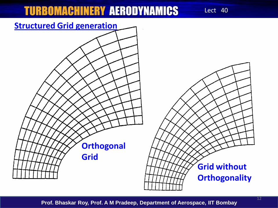
Orthogonal Grid
Grid without Orthogonality
Structured Grid generation
13Prof. Bhaskar Roy, Prof. A M Pradeep, Department of Aerospace, IIT Bombay
Lect 40
13
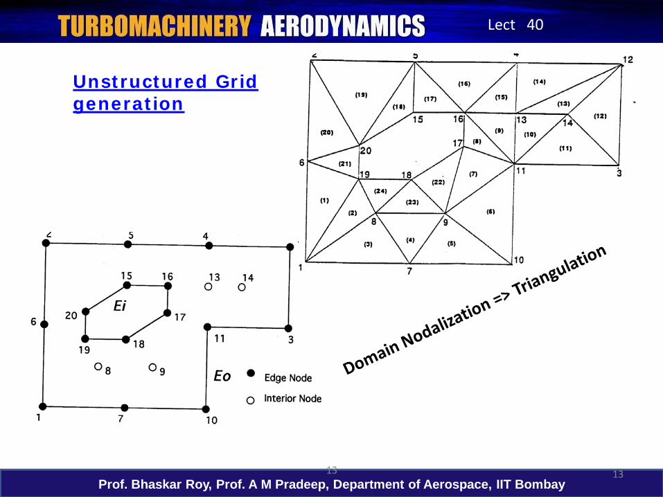
Unstructured Grid generation
14Prof. Bhaskar Roy, Prof. A M Pradeep, Department of Aerospace, IIT Bombay
Lect 40
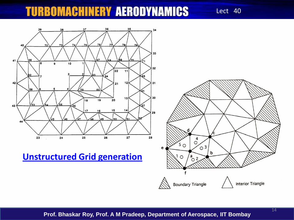
Unstructured Grid generation

15Prof. Bhaskar Roy, Prof. A M Pradeep, Department of Aerospace, IIT Bombay
Lect 40
CFD in Blade Design
16Prof. Bhaskar Roy, Prof. A M Pradeep, Department of Aerospace, IIT Bombay
Lect 40
16
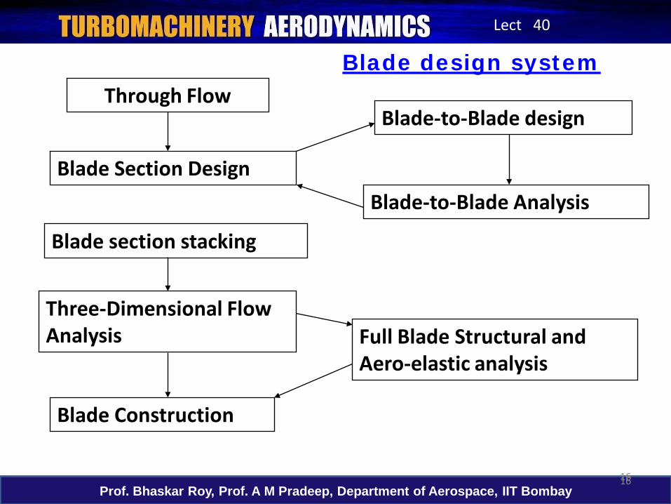
Through Flow
Blade Section Design
Blade section stacking
Three-Dimensional Flow Analysis
Blade-to-Blade design
Blade-to-Blade Analysis
Blade Construction
Full Blade Structural and Aero-elastic analysis
Blade design system

17Prof. Bhaskar Roy, Prof. A M Pradeep, Department of Aerospace, IIT Bombay
Lect 40
Through Flow Program
Input : a) i) Annulus Information ii) Blade row exit informationiii) Inlet profiles of Pr, Temp, a1iv) Inlet Mass flow v) Rotational speeds of rotorsvi) Blade geometry, Loss distributionsvii) Passage averaged perturbation
terms
Output : b) i) Blade row inlet and exit conditionsii) Streamline definition and streamtube
height
18Prof. Bhaskar Roy, Prof. A M Pradeep, Department of Aerospace, IIT Bombay
Lect 40
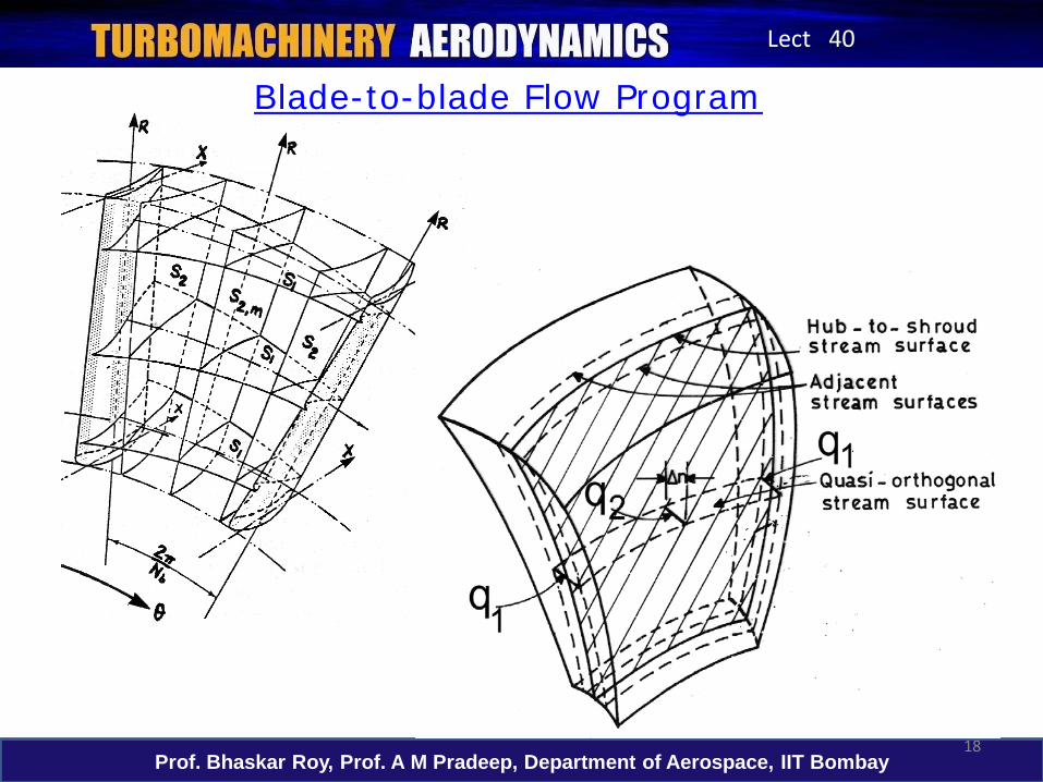
Blade-to-blade Flow Program

19Prof. Bhaskar Roy, Prof. A M Pradeep, Department of Aerospace, IIT Bombay
Lect 40
Blade-to-blade Flow Program

20Prof. Bhaskar Roy, Prof. A M Pradeep, Department of Aerospace, IIT Bombay
Lect 40
Blade-to-Blade program
Input : Blade geometryInlet and Exit Velocity
distributionStreamline Definition
Output : Surface velocity distributionProfile and loss distribution
Section Stacking Program
Input : Blade section geometryStacking points and stacking lineAxial and Tangential leans (sweep
and Dihedral)Output : Three-Dimensional blade geometry

21Prof. Bhaskar Roy, Prof. A M Pradeep, Department of Aerospace, IIT Bombay
Lect 40
19 21
2D MISES code for Cascade Analysis
Blade-to-Blade program

22Prof. Bhaskar Roy, Prof. A M Pradeep, Department of Aerospace, IIT Bombay
Lect 40
2D MISES code for Cascade Analysis Cp contour
23Prof. Bhaskar Roy, Prof. A M Pradeep, Department of Aerospace, IIT Bombay
Lect 40
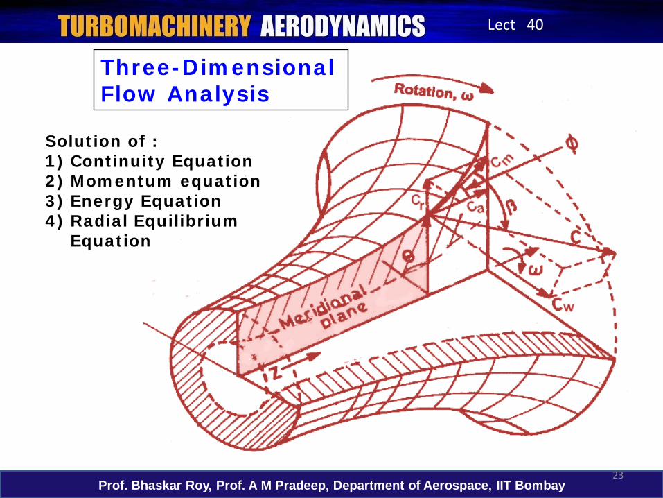
Three-Dimensional Flow Analysis
Solution of : 1) Continuity Equation2) Momentum equation3) Energy Equation4) Radial Equilibrium
Equation
24Prof. Bhaskar Roy, Prof. A M Pradeep, Department of Aerospace, IIT Bombay
Lect 40
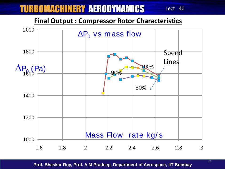
1000
1200
1400
1600
1800
2000
1.6 1.8 2 2.2 2.4 2.6 2.8 3
Mass Flow rate kg/s
ΔP0 vs mass flow
∆P0 (Pa)
80%
90%
Speed Lines
100%
Final Output : Compressor Rotor Characteristics
25Prof. Bhaskar Roy, Prof. A M Pradeep, Department of Aerospace, IIT Bombay
Lect 40
Thank you
for
participating in this NPTEL course