least-squares seismic migration using · pdf filedraft: october 3, 2003 14:01 file:...

DRAFT: October 3, 2003 14:01 File: kuehl-sacchi pp.307–329 Page 307 Sheet 1 of 23

CANADIAN APPLIED

MATHEMATICS QUARTERLY

Volume 10, Number 2, Summer 2002

LEAST-SQUARES SEISMIC MIGRATION

USING WAVEFIELD PROPAGATORS

FOR AVP INVERSION

Based on a presentation at the PIMS–MITACS Workshop on

Inverse Problems and Imaging, University of British Columbia,

June 9–10, 2001.

HENNING KUEHL AND MAURICIO D. SACCHI

ABSTRACT. The imaging of geological subsurface struc-tures with seismic reflection energy is a powerful tool for thedetection and the assessment of hydrocarbon reservoirs. Theseismic method can be understood as a multi-source and multi-receiver reflection scattering experiment. The seismic sourcesand receivers are placed at the earth’s surface. The sources emitseismic energy into the subsurface and the receivers record theearth’s response (the backscattered energy) as a function oftime and position relative to the source. The goal of seismicimaging is to invert the recorded seismograms for the subsurfacestructures and their underlying lithological properties. Seismic

imaging is usually called migration when only structural imageinformation is desired. The term inversion is used if the goalis to invert for physical properties of the subsurface. In thispaper, we do not attempt to invert for true physical param-eters. Instead, we aim at preserving the angle or the closelyrelated ray-parameter dependence of migrated seismic data. Ina subsequent step, this information can then be used to invertfor the lithological parameters that determine the angle/ray-parameter dependent subsurface reflectivity. In the frameworkof linearized scattering theory seismic data modelling and mi-gration is defined as a pair of adjoint operators. This definitionleads to the formulation of an iterative least-squares seismicmigration method. The modelling/migration operator pair isimplemented using a wavefield propagator technique. We pro-pose least-squares migration with a regularization term thatimposes continuity on amplitude variations as a function ofray-parameter (AVP). This regularization is based on the idea

AMS subject classification: 86A15.Copyright c©Applied Mathematics Institute, University of Alberta.

307


308 HENNING KUEHL AND MAURICIO D. SACCHI

that roughness along the ray-parameter axis stems from nu-merical artifacts and incompletely and/or irregularly sampledseismic wavefields. A synthetic seismic data example is givenfor illustration.

1 Introduction. Most common seismic imaging techniques can besubdivided into two categories. The first category are algorithms thatback-propagate the seismic surface wavefield into the earth using recur-sive propagators. These algorithms are frequently called wave-equationmigration/inversion techniques. The second category are algorithmsbased on ray-tracing. They are often referred to as Kirchhoff-type imag-ing techniques. In ray-tracing, problems with shadow zones and causticscan occur depending on the complexity of the geology of the subsurface.Furthermore, the ability of the ray-based approach to account for multi-pathing is limited. Propagator techniques, on the other hand, allowthe seismic waves to travel along all possible ray-paths (Gray and May,[11]).

The formulation of migration/inversion algorithms starts with thedefinition of a subsurface model in terms of physical parameters and areflection scattering mechanism. To make the imaging problem tractablewe make simplifying assumptions about the model and its interactionswith the seismic wavefield. Based on the work of Clayton and Stolt [6],we then derive a forward modelling formula that relates the adoptedsubsurface model with the seismic data. The ultimate goal in migra-tion/inversion is to solve the forward relationship for the unknown sub-surface model parameters. However, we must keep in mind that, inpractice, our simplified model serves merely as a proxy for the moregeneral nature of the problem. We must therefore interpret the resultswith care.

In order to invert the generally “ill-posed” problem we employ a least-squares data fitting method. This allows us to regularize the least-squares solution by imposing certain desirable characteristics and con-straints.

Nemeth et al. [20] and Duquet et al. [8] followed the least-squaresapproach to obtain Kirchhoff-type least-squares imaging techniques. Inthis paper we investigate the possibility of using wavefield propagatorsinstead.

In the first part of this paper, we briefly review seismic data mod-elling based on linear scattering theory. Furthermore, we discuss the useof Green’s functions for seismic modelling in spatially varying referencemedia. This leads to a linear operator equation that relates the subsur-

DRAFT: October 3, 2003 14:01 File: kuehl-sacchi pp.307–329 09 Sheet 3 of 23

LEAST-SQUARES SEISMIC MIGRATION 309

face reflectivity with the seismic data. This review is mostly based on apaper by Stolt and Weglein [26].

Next, we introduce a phase-shift propagator method to computeGreen’s functions in laterally invariant media that is described in Clay-ton and Stolt [6].

The computation of the least-squares inverse requires the knowledgeof the adjoint of the modelling operator. The adjoint operator can beregarded as a first approximation to the inverse problem (Claerbout, [5]).In fact, applying the adjoint operator is often sufficient for structuralimaging. In this paper we define migration as the adjoint of modelling.Following Stolt and Weglein [26] we describe how to extract amplitudevariation with angle (AVA) information from the migrated wavefield.

Since propagator techniques are most beneficial when applied to imag-ing problems in complex environments, the modelling/migration opera-tors are generalized for laterally varying media. This can be achieved byexpanding the operators used by Clayton and Stolt [6]. The expansionwe adopt here results in extended split-step propagators for modellingand migration (Gazdag and Sguazzero, [10]; Stoffa et al., [25]; Kessinger,[13]; Margrave and Ferguson, [18]).

As an alternative to AVA imaging/inversion one can use the offsetray-parameter to obtain amplitude variation with ray-parameter (AVP)information (de Bruin et al., [7]; Prucha et al., [23]; Mosher and Foster,[19]). In this paper we will choose the AVP over the AVA parameteri-zation.

To complete the discussion on migration using AVP imaging we brieflymention the possibility to improve the adjoint operator by consideringthe so-called imaging Jacobian (Stolt and Benson, [27]; Sava et al., [24]).The analytical imaging Jacobian can also be used to precondition theiterative least-squares migration discussed in the last part.

In least-squares migration we use the above generalized modelling/migration operators to formulate a least-squares migration/inversionscheme. We introduce a regularization of the inverse problem thatappears particularly beneficial when the emphasis is on obtaining am-plitude variation with ray-parameter (AVP) information. An examplebased on the synthetic Marmousi data set (Versteeg and Grau, [28]) isgiven for illustration.

2 Seismic data modelling under the Born approximation.

Consider the 3-D acoustic wave-equation with variable density ρ(x) and



compressional velocity α(x) in the frequency domain:

D(x, ω)Ψ(x, s, ω) =

(

∇ · 1

ρ(x)∇ +

ω2

ρ(x)α2(x)

)

Ψ(x, s, ω)

= −δ(x− s),

(1)

where the time-dependence of the wavefield Ψ(x, s, ω) is given by e−iωt.The operator D(x, ω) is the variable density Helmholtz operator. Thevector x = (x, y, z) denotes the spatial position in a coordinate systemwith the positive z component pointing down into the earth (Figure 1).The vector s is the position of the point source and the compressionalvelocity α(x) and density ρ(x) are spatially varying. We define the bulk-modulus K(x) = ρ(x)α2(x) and follow Stolt and Weglein [26] and castthe problem as a perturbation about a reference solution by introducingthe reference operator D0:

(2) D0(x, ω) = ∇ · 1

ρ0(x)∇ +

ω2

K0(x),

where K0(x) and ρ0(x) are slowly varying local averages of the truevalues K(x) and ρ(x), too slowly varying to produce significant reflectionenergy.

The scattering operator (scattering potential) V(x, ω) that generatesthe seismic reflection data is defined as:

V(x, ω) = D(x, ω) −D0(x, ω)

= ∇ ·(

1

ρ(x)− 1

ρ0(x)

)

∇ + ω2

(

1

K(x)− 1

K0(x)

)

= ∇ ·(

a2(x)

ρ0(x)

)

∇ + ω2

(

a1(x)

K0(x)

)

,

(3)

where a1(x) = ρ0(x)ρ(x) − 1 = ∆ρ(x)

ρ(x) and a2(x) = K0(x)K(x) − 1 = ∆K(x)

K(x) .

The coefficients a1(x) and a2(x) are unknown fractional changes of themedium properties describing the subsurface. The differential operatorsin the term containing a2 cause an angle dependence of the scatteringpotential.

We substitute D = V + D0 in equation (1) and obtain:

(4) D0Ψ(x, s) = −VΨ(x, s) − δ(x − s).



V(x)

z < 0V(x)=0

z > 0

xy

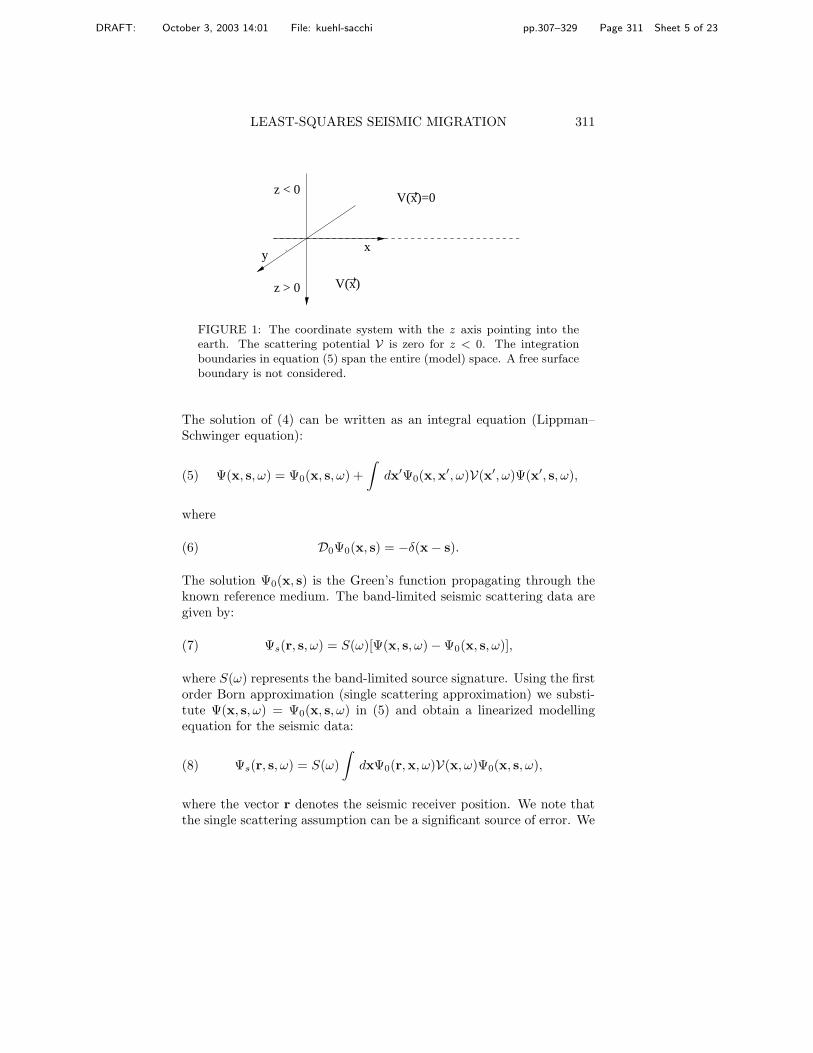
FIGURE 1: The coordinate system with the z axis pointing into theearth. The scattering potential V is zero for z < 0. The integrationboundaries in equation (5) span the entire (model) space. A free surfaceboundary is not considered.

The solution of (4) can be written as an integral equation (Lippman–Schwinger equation):

(5) Ψ(x, s, ω) = Ψ0(x, s, ω) +

∫

dx′Ψ0(x,x′, ω)V(x′, ω)Ψ(x′, s, ω),

where

(6) D0Ψ0(x, s) = −δ(x − s).

The solution Ψ0(x, s) is the Green’s function propagating through theknown reference medium. The band-limited seismic scattering data aregiven by:

(7) Ψs(r, s, ω) = S(ω)[Ψ(x, s, ω) − Ψ0(x, s, ω)],

where S(ω) represents the band-limited source signature. Using the firstorder Born approximation (single scattering approximation) we substi-tute Ψ(x, s, ω) = Ψ0(x, s, ω) in (5) and obtain a linearized modellingequation for the seismic data:

(8) Ψs(r, s, ω) = S(ω)

∫

dxΨ0(r,x, ω)V(x, ω)Ψ0(x, s, ω),

where the vector r denotes the seismic receiver position. We note thatthe single scattering assumption can be a significant source of error. We



P

θnP

Ph

s

r

Pm

local reflector element

RS

θ

Φ

Γs Γr

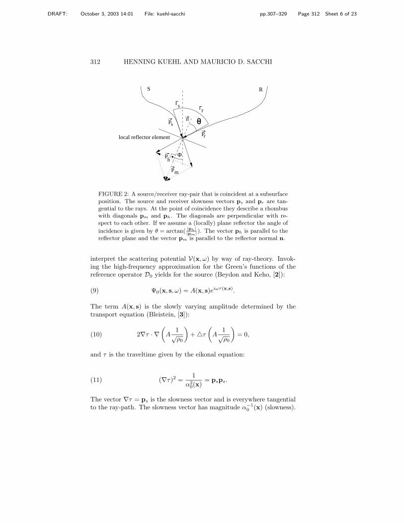
FIGURE 2: A source/receiver ray-pair that is coincident at a subsurfaceposition. The source and receiver slowness vectors ps and pr are tan-gential to the rays. At the point of coincidence they describe a rhombuswith diagonals pm and ph. The diagonals are perpendicular with re-spect to each other. If we assume a (locally) plane reflector the angle of

incidence is given by θ = arctan( |ph||pm|

). The vector ph is parallel to thereflector plane and the vector pm is parallel to the reflector normal n.

interpret the scattering potential V(x, ω) by way of ray-theory. Invok-ing the high-frequency approximation for the Green’s functions of thereference operator D0 yields for the source (Beydon and Keho, [2]):

(9) Ψ0(x, s, ω) = A(x, s)eiωτ(x,s).

The term A(x, s) is the slowly varying amplitude determined by thetransport equation (Bleistein, [3]):

(10) 2∇τ · ∇(

A1√ρ0

)

+ 4τ

(

A1√ρ0

)

= 0,

and τ is the traveltime given by the eikonal equation:

(11) (∇τ)2 =1

α20(x)

= psps.

The vector ∇τ = ps is the slowness vector and is everywhere tangentialto the ray-path. The slowness vector has magnitude α−1

0 (x) (slowness).



The functions τ and A must also satisfy τ = 0 for x = s and |x− s|A →1/4π, as x → s (Bleistein, [3]).

Using the high frequency approximation in equation (8) and integra-tion by parts yields:

(12) Ψs(r, s, ω) = ω2S(ω)

∫

dxA(r,x)A(x, s)v(x, θ)

K0(x)eiw(τ(x,r)+τ(x,s)),

where:

(13) v(x, θ) = a1(x) + cos(2θ)a2(x).

The angle 2θ is the angle between the local source slowness vector ps

and the local receiver slowness vector pr at the depth-point where thetwo ray-paths coincide (Figure 2). The source and receiver slownessvectors describe a rhombus with diagonals pm = pr + ps and ph =pr − ps. If we interpret the reflection scattering to be caused by a(locally) plane reflector (specular reflection), the diagonals are directlyrelated to reflector dip Φ and angle of incidence θ as demonstrated inFigure 2. As we shall see later, the vectors pm and ph are also relatedto the midpoint-offset domain, a coordinate system frequently used inseismic processing.

For simplicity we restrict the theory to the two-dimensional case. Ifwe assume a line source and invariant medium properties along the ydirection, equation (12) simplifies to:1

Ψs(r, 0|s, 0, ω) = ω2S(ω)

∫∫

dx dzA(r, 0|x, z)A(x, z|s, 0)

× v(x, z, θ)

K0(x, z)eiw(τ(x,z|r,0)+τ(x,z|s,0)) ,

(14)

where we have switched from the vector to a coordinate notation. Fur-thermore, we assume that sources and receivers are placed along a leveldatum at z = 0. Equation (14) can be implemented by calculatingthe amplitude terms and traveltimes numerically using a (paraxial) ray-tracing algorithm (Beydon and Keho, [2]). However, here we wouldlike to employ a wavefield propagator technique. We abandon the ray-theoretical Green’s functions and write equation (14) again in the more

1Strictly speaking, this formula is only valid when applied to synthetic data basedon the two dimensional wave-equation. When dealing with real-world data 2 1

2-D

effects should be considered (Stolt and Weglein, [26]; Bleistein, [3]).



general form:

Ψs(r, 0|s, 0, ω)

= ω2S(ω)

∫∫

dx dzΨ0(r, 0|x, z, ω)v(x, z, θ)

K0(x, z)Ψ0(x, z|s, 0, ω).

(15)

The interpretation of the interaction between the reflector element andthe wavefield remains valid since it involves only local quantities at thereflection point.

2.1 Modelling using propagators in laterally invariant refer-

ence media. For laterally invariant reference media the Green’s func-tions in equation (15) can be replaced by the WKBJ Green’s functionobtained for the depth-separated wave equation (Clayton and Stolt, [6]).The depth separation is achieved by Fourier transforms along the hori-zontal coordinates in equation (6). The Green’s function for the sourcehas the analytical expression (Clayton and Stolt, [6]):(16)

Ψ0(x, z|s, 0, ω) =

√

ρ0(z)ρ0(0)

2π

∫

dksxeiksx(s−x) ieiω∫

z

0psz(z′) dz′

2ω√

psz(z)psz(0),

where psz is the vertical receiver slowness component. The vertical slow-ness component is calculated from the horizontal source wavenumber ksx

and the dispersion relation of the wave equation:

(17) ωpsz(z) = ksz(z) =ω

α0(z)

√

1 − k2sxα2

0(z)

ω2,

where ksz(z) is the vertical source wavenumber. The receiver Green’sfunction is obtained in an analogous way. Inserting the Green’s func-tions in (15) gives the modelling formula in the frequency-wavenumber(Clayton and Stolt, [6]; Stolt and Benson, [27]):2

Ψs(krx, 0|ksx, 0, ω) = −ω2S(ω)

∫

dzρ0(0)ρ0(z)

4√

krz(0)krz(z)ksz(0)ksz(z)

× v(krx + ksx, z, θ)

K0(krx + ksx, z, θ)ei

∫

z

0krz(z′)+ksz(z′) dz′

.

(18)

2Rather than defining new symbols when a function is transformed to a newdomain, we use the same symbol with the new arguments.



ks = (ksx, ksz) kr = (krx, krz)

ps = ks

ωpr = kr

ω

ps = (sin Γs,cos Γs)α0

pr = (sin Γr,cos Γr)α0

km = ks + kr kh = kr − ks

pm = km

ωph = kh

ω

ks = 1/2(km − kh) kr = 1/2(km + kh)

ksz = ωα0

√

1 − α2

0k2

sx

ω2 krz = ωα0

√

1 − α2

0k2

rx

ω2

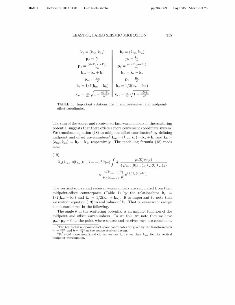
TABLE 1: Important relationships in source-receiver and midpoint-offset coordinates.

The sum of the source and receiver surface wavenumbers in the scatteringpotential suggests that there exists a more convenient coordinate system.We transform equation (18) to midpoint offset coordinates3 by definingmidpoint and offset wavenumbers4 km = (kmx, kz) = ks + kr and kh =(khx, khz) = kr − ks, respectively. The modelling formula (18) readsnow:

Ψs(kmx, 0|khx, 0, ω) = −ω2S(ω)

∫

dzρ0(0)ρ0(z)

4√

krz(0)krz(z)ksz(0)ksz(z)

× v(kmx, z, θ)

K0(kmx, z, θ)ei

∫

z

0kz(z′) dz′

.

(19)

The vertical source and receiver wavenumbers are calculated from theirmidpoint-offset counterparts (Table 1) by the relationships ks =1/2(km − kh) and kr = 1/2(km + kh). It is important to note thatwe restrict equation (19) to real values of kz . That is, evanescent energyis not considered in the following.

The angle θ in the scattering potential is an implicit function of themidpoint and offset wavenumbers. To see this, we note that we havepm · ph = 0 at the point where source and receiver rays are coincident.

3The horizontal midpoint-offset space coordinates are given by the transformationm = r+s

2and h = r−s

2at the source-receiver datum.

4To avoid more notational clutter we use kz rather than kmz for the verticalmidpoint wavenumber.



From Figure 2 we find (Stolt and Weglein, [26]):

(20) tan θ =|ph||pm| =

phx

pmz

=khx

kz

.

The ray-parameters in (20) are understood to be taken at the reflectionpoint.

The horizontal slowness components are constant along the rays, sincethere are no lateral velocity variations in the reference medium. This factcan be used to formulate modelling/migration algorithms that operatedirectly in the horizontal offset ray-parameter domain (Ottolini, [21]).However, we will drop this assumption further below which will makethe recalculation of the horizontal wavefield spectrum at each depth levelinevitable.

To simplify the notation the data modelling formula (19) is writtenin terms of a symbolic operator notation. First we define an angle-dependent model function f by:

(21) f(

kmx,khx

kz

, z)

=−ω2v

(

kmx, z, arctan(khx

kz

))

K0

(

kmx, z, arctan(khx

kz

)) .

This function is made suitable for wavefield propagation by mappingf(kmx, khx

kz

, z) to f(kmx, khx, z) in a preparation step prior to modelling:

(22) f(kmx, khx, z) = F−1z R′

θFzf(

kmx,khx

kz

, z)

,

where Fz and F−1z are the forward and inverse Fourier transform along z,

respectively. The operator R′θ is the adjoint of the radial-trace transform

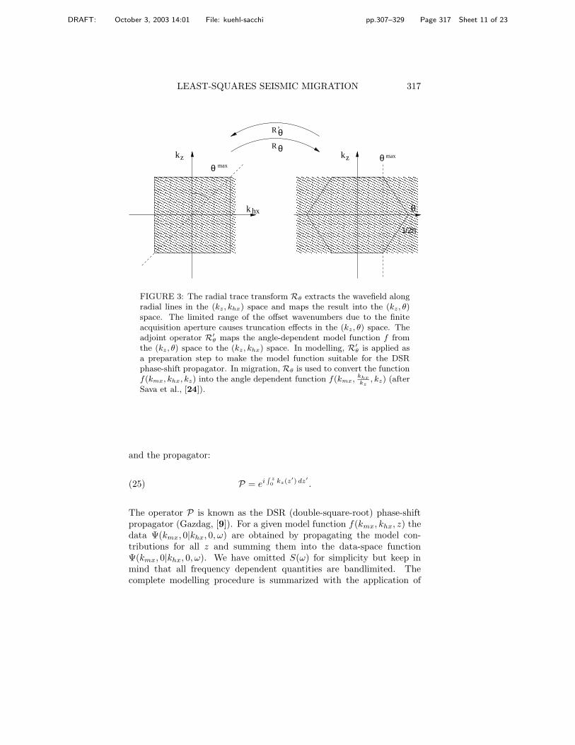
Rθ from the (kz, khx) to (kz, θ) space.5 This mapping procedure isillustrated in Figure 3.

The forward modelling operation is now written symbolically as:

(23) Ψ(kmx, 0|khx, 0, ω) =

∫

dzAPf(kmx, khx, z),

with the diagonal WKBJ amplitude scaling operator:

(24) A =ρ0(0)ρ0(z)

4√

krz(0)krz(z)ksz(0)ksz(z)5The radial-trace transform Rθ is equivalent to the more intuitive slant-stack

(Ottolini, 1984) in the offset-depth domain.



��

��

��

��

k

1/2π

θhx

R

R

’

θθ max

maxzk zk

θ

θ

FIGURE 3: The radial trace transform Rθ extracts the wavefield alongradial lines in the (kz, khx) space and maps the result into the (kz, θ)space. The limited range of the offset wavenumbers due to the finiteacquisition aperture causes truncation effects in the (kz, θ) space. Theadjoint operator R

′θ maps the angle-dependent model function f from

the (kz, θ) space to the (kz, khx) space. In modelling, R′θ is applied as

a preparation step to make the model function suitable for the DSRphase-shift propagator. In migration, Rθ is used to convert the functionf(kmx, khx, kz) into the angle dependent function f(kmx, khx

kz, kz) (after

Sava et al., [24]).

and the propagator:

(25) P = ei∫

z

0kz(z′) dz′

.

The operator P is known as the DSR (double-square-root) phase-shiftpropagator (Gazdag, [9]). For a given model function f(kmx, khx, z) thedata Ψ(kmx, 0|khx, 0, ω) are obtained by propagating the model con-tributions for all z and summing them into the data-space functionΨ(kmx, 0|khx, 0, ω). We have omitted S(ω) for simplicity but keep inmind that all frequency dependent quantities are bandlimited. Thecomplete modelling procedure is summarized with the application of



the operator L:

Ψ(kmx, 0|khx, 0, ω) =

∫

dzPF−1z R′

θFzf(

kmx,khx

kz

, z)

= Lf(

kmx,khx

kz

, z)

.(26)

Notice that we have conveniently dropped the scaling factor A in equa-tion (26). In fact, Wapenaar [30] shows that this is justified, since theemployed Green’s function should be normalized with respect to the en-ergy flux across interfaces separating regions of different medium param-eters. Effectively, energy flux normalization amounts to a cancellationof the WKBJ amplitude term A and warrants that seismic reciprocityis honored (Wapenaar, [30]).

3 Seismic migration. Our goal is to invert the seismic data forthe angle dependence of f(kmx, khx

kz

, z). The function f is determinedby the two unknowns a1 and a2. Here, we are just concerned withproducing an estimate of the amplitude variation with incident angle(AVA) of f(kmx, khx

kz

, z). In fact, the relevance of the quantities a1 anda2 for seismic inversion is debatable (Wapenaar, [29]). Seismic data aremostly generated by reflecting interfaces. For a plane wave incident ona plane reflecting interface in an elastic medium the Zoeppritz equa-tions determine the amplitude behavior as a function of angle (Aki andRichards, 1980). Stolt and Weglein [26] relate the scattering potential tothe linearized Zoeppritz equation (Aki and Richards, [1]) for the reflec-tion of a compressional wave on a plane interface. However, to achievethis they introduce additional scaling factors and a normal derivative tobe applied during inversion. Instead, Wapenaar [29] demonstrates thatthese steps are not necessary and that the scattering potential can beidentified directly with the reflection coefficient for specularly reflectedcompressional waves. That is, the particular form of the scattering po-tential is merely an artifact of the linear Born approximation and, forspecular reflections, can be replaced ad hoc by the specular reflectivityfunction (Bleistein et al., [4]). However, we must keep in mind that theassumption of a low contrast medium due to the linear Born approx-imation (weak scattering) is implicit in our formulas. This is becausetransmission loss due to energy partitioning at the interfaces and mul-tiple scattering are not accounted for.

In any case, the function f(kmx, khx

kz

, z) exhibits angle dependence andthe migration/inversion should attempt to preserve this dependence as



faithfully as possible. Ideally, we would like to carry out the inversion forf(kmx, khx

kz

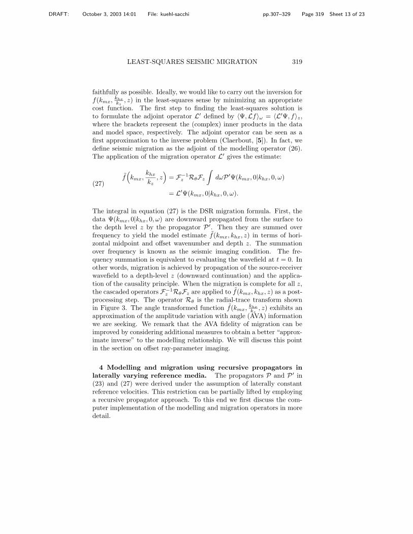
, z) in the least-squares sense by minimizing an appropriatecost function. The first step to finding the least-squares solution isto formulate the adjoint operator L′ defined by 〈Ψ,Lf〉ω = 〈L′Ψ, f〉z,where the brackets represent the (complex) inner products in the dataand model space, respectively. The adjoint operator can be seen as afirst approximation to the inverse problem (Claerbout, [5]). In fact, wedefine seismic migration as the adjoint of the modelling operator (26).The application of the migration operator L′ gives the estimate:

f̃(

kmx,khx

kz

, z)

= F−1z RθFz

∫

dωP ′Ψ(kmx, 0|khx, 0, ω)

= L′Ψ(kmx, 0|khx, 0, ω).

(27)

The integral in equation (27) is the DSR migration formula. First, thedata Ψ(kmx, 0|khx, 0, ω) are downward propagated from the surface tothe depth level z by the propagator P ′. Then they are summed overfrequency to yield the model estimate f̃(kmx, khx, z) in terms of hori-zontal midpoint and offset wavenumber and depth z. The summationover frequency is known as the seismic imaging condition. The fre-quency summation is equivalent to evaluating the wavefield at t = 0. Inother words, migration is achieved by propagation of the source-receiverwavefield to a depth-level z (downward continuation) and the applica-tion of the causality principle. When the migration is complete for all z,the cascaded operators F−1

z RθFz are applied to f̃(kmx, khx, z) as a post-processing step. The operator Rθ is the radial-trace transform shownin Figure 3. The angle transformed function f̃(kmx, khx

kz

, z) exhibits anapproximation of the amplitude variation with angle (AVA) informationwe are seeking. We remark that the AVA fidelity of migration can beimproved by considering additional measures to obtain a better “approx-imate inverse” to the modelling relationship. We will discuss this pointin the section on offset ray-parameter imaging.

4 Modelling and migration using recursive propagators in

laterally varying reference media. The propagators P and P ′ in(23) and (27) were derived under the assumption of laterally constantreference velocities. This restriction can be partially lifted by employinga recursive propagator approach. To this end we first discuss the com-puter implementation of the modelling and migration operators in moredetail.



In a numerical implementation the integrals in the phase-shift opera-tors of (23) and (27) are replaced by summations and dz becomes a finitedepth interval ∆z. The velocities are assumed to be constant along thevertical range ∆z. The phase-shift propagator can then be implementedas a non-recursive or recursive algorithm. In the non-recursive imple-mentation the propagation between the surface-data and the depth-levelz is carried out by computation of the complete phase-integral prior topropagation. In the recursive implementation the wavefield is succes-sively propagated by iterative application of the phase-shift propagatorin steps ∆z.

Both implementations have certain advantages and disadvantages.Beneficial consequences of the non-recursive implementation are demon-strated in Kuehl and Sacchi [15]. However, in order to accommodatelateral velocity variations we must implement the modelling and mi-gration formulas as recursive algorithms. This allows us to extend thephase-shift propagator by a local operator expansion. To this end weexpand the square-root expression for the vertical source wavenumberin (17) using the split-step approximation (Stoffa et al., [25]). For thesource we have:

(28) ksz(s, z) ≈√

ω2

α20 ref(z)

− k2sx +

(

ω

α0(s, z)− ω

α0 ref(z)

)

.

The same approximation is used for the receiver square-root operator.The reference velocity α0 ref(z) is computed by laterally averaging theslowness variations for each propagation step ∆z. The additional termin (28) is the split-step correction. It is applied at the source and receiverlocations after the wavefield has been transformed to the space domain.This results in a recursive marching algorithm that alternates betweenthe horizontal wavenumber and space domain at each depth level. Thistype of algorithm is known to give relatively accurate structural imageseven in complex media (Popovici, [22]).

The wide-angle accuracy of the split-step approximation can be im-proved by using multiple reference velocities for the propagation. Thephase-shift propagators and the split-step correction are then applied ina data windowing mode (Gazdag and Sguazzero, [10]; Kessinger, [13];Margrave and Ferguson, [18]). The standard and the windowed split-step approach can be applied to both the modelling and the migrationoperator.



5 Modelling and migration with the offset ray-parameter.

One may ask how meaningful the interpretation of θ as the “angle ofincidence” really is. In seismic imaging/inversion one deals mostly withregular geological interfaces. So one would like to relate the scatteringpotential to the reflectivity of the interfaces and interpret the angle θ asthe local angle of incidence. For this interpretation to be true, the inter-face curvature has to be moderate so that the reflection mechanism ispredominantly specular. Furthermore, the conversion to “angle of inci-dence” is dependent on the reference velocity model (migration velocityfield), since the vertical wavenumber is a function of α0. Unfortunately,the reference velocity is only known roughly in general. In practice, AVAestimation is an interpretive process and breaks down in areas where theabove conditions are not fulfilled.

��

��

��

��

Σ,

k hx

R’

Rω

p

p

phx

Σ

ωp

hxmax

phxmax

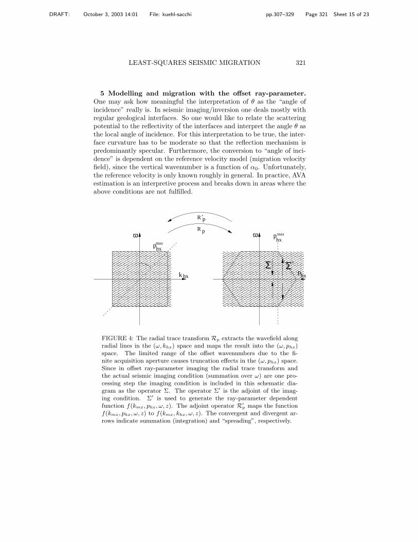
FIGURE 4: The radial trace transform Rp extracts the wavefield alongradial lines in the (ω, khx) space and maps the result into the (ω, phx)space. The limited range of the offset wavenumbers due to the fi-nite acquisition aperture causes truncation effects in the (ω, phx) space.Since in offset ray-parameter imaging the radial trace transform andthe actual seismic imaging condition (summation over ω) are one pro-cessing step the imaging condition is included in this schematic dia-gram as the operator Σ. The operator Σ′ is the adjoint of the imag-ing condition. Σ′ is used to generate the ray-parameter dependentfunction f(kmx, phx, ω, z). The adjoint operator R

′p maps the function

f(kmx, phx, ω, z) to f(kmx, khx, ω, z). The convergent and divergent ar-rows indicate summation (integration) and “spreading”, respectively.



The uncertainty with respect to reference velocity field motivates analternative approach to angle imaging. Instead of “angle of incidence” weuse the horizontal offset ray-parameter to obtain an amplitude variationwith ray-parameter (AVP) estimate of the subsurface (de Bruin et al.,[7]; Prucha and Biondi, [23]; Mosher and Foster, [19]). This is achievedby parameterizing the model function f with phx = khx

ωand by using

the relation θ = arcsin( α0phx

2 cos Φ) (see Figure 2): f(kmx, khx

ω, Φ, z). The

dip angle Φ of the reflector element is now an implicit parameter ofthe model function f and is omitted in the following for convenience.A conversion from AVP to AVA requires the dip angle Φ as an inputparameter that is provided by an interpreter. The dip is measured onthe structural image. Hence, we do not rely on the reference velocityfield for the local dip information. This extra step could, in some cases,help to improve the robustness of AVA estimation.

The offset ray-parameter is a quantity belonging to the data space andnot the model space. This is because of the ω dependence of phx. In orderto perform modelling we first map f(kmx, khx

ω, z) to f(kmx, khx, ω, z):

(29) f(kmx, khx, ω, z) = R′pf

(

kmx,khx

ω, z

)

.

This mapping results in the “spreading” of the values f(kmx, khx

ω, z)

along the ω axis (Figure 4). The subsequent transform R′p is the adjoint

of the radial trace transformation from the (ω, khx) to the (ω, phx) spaceas shown in Figure 4.

The modelling is completed by applying the DSR propagator andsumming the contribution of all depth levels into the data function:

(30) Ψ(kmx, 0|khx, 0, ω) =

∫

dzPf(kmx, khx, ω, z).

We note that the conversion from the model to the data space wasachieved implicitly in equation (29). As opposed to the previously out-lined AVA mapping, the ray-parameter conversion is absorbed in themodelling process. We write (29) and (30) in one symbolic operatorequation:(31)

Ψ(kmx, 0|khx, 0, ω) =

∫

dzPR′pf

(

kmx,khx

ω, z

)

= Lf(

kmx,khx

ω, z

)

.

The migration formula is again found by formulating the adjoint opera-



tor:

f̃(

kmx,khx

ω, z

)

=

∫

dwRpP ′Ψ(kmx, 0|khx, 0, ω)

= L′Ψ(kmx, 0|khx, 0, ω).

(32)

Again we can choose a recursive implementation of (31) and (32) andemploy the (generalized) split-step operator expansion to make formulassuitable for laterally varying media.

The modelling/migration operator pair (31) and (32) is used in thenext section to invert seismic data in the least-squares sense. If insteadonly the adjoint (migration) operator (32) is to be applied the approxi-mation of the inverse problem can be improved as shown by Sava et al.[24]. Their technique involves the computation of the local imagingJacobian J = dω

dkz

|z (Stolt and Benson, [27]). For AVP imaging, thevertical wavenumber kz must be expressed as a function of offset ray-parameter. The resulting diagonal operator Jp evaluated at depth zis used by Sava et al. [24] to obtain an analytical approximate inverseoperator:

f̃inv

(

kmx,khx

ω, z

)

=

∫

dwJ−1p RpP ′Ψ(kmx, 0|khx, 0, ω)

= L′invΨ(kmx, 0|khx, 0, ω).

(33)

However, this approximation is not satisfactory if the inversion is plaguedwith, for instance, incomplete data sampling and numerical operator ar-tifacts.

6 Least-squares migration for AVP imaging. In least-squaresmigration/inversion we use the modelling and migration operators toinvert the linear system (Kuehl and Sacchi, [16]):

(34) Ψ(m, 0|h, 0, ω) = Lf(m, phx, z) + n,

where Ψ(m, 0|h, 0, ω) is the often incomplete seismic data in the mid-point-offset space-domain and n represents the noise. The function fis the ray-parameter dependent model function in midpoint-depth co-ordinates. The operator L now includes forward and backward Fouriertransforms for midpoint and offset.



The following cost function is iteratively minimized by a gradientmethod (Hestenes and Stiefel, [12]):

F (f) =∥

∥W(

Ψ(m, 0|h, 0, ω) − Lf(m, phx, z))∥

∥

2

+ λ2‖∂phxf(m, phx, z)‖2,

(35)

where W is a diagonal weighting operator. The operator W is derivedfrom the data covariance matrix and has zero weights in the case of deadtraces and non-zero weights for live traces (Kuehl and Sacchi, [14]). Theminimization amounts to an iterative application of L′ and L. Besidesthe data-misfit term, we have added a regularization term that penal-izes “roughness” along the ray-parameter phx. The λ2 factor allows usto control the amount of smoothing. The concept of smoothing is basedon the desire to retrieve a continuous function f along the ray-parameteraxis. This is justified by the logic that the angle/ray-parameter depen-dence should be continuous. Discontinuities or rapid amplitude changesare attributed to missing data (data aliasing) and numerical operatorartifacts.

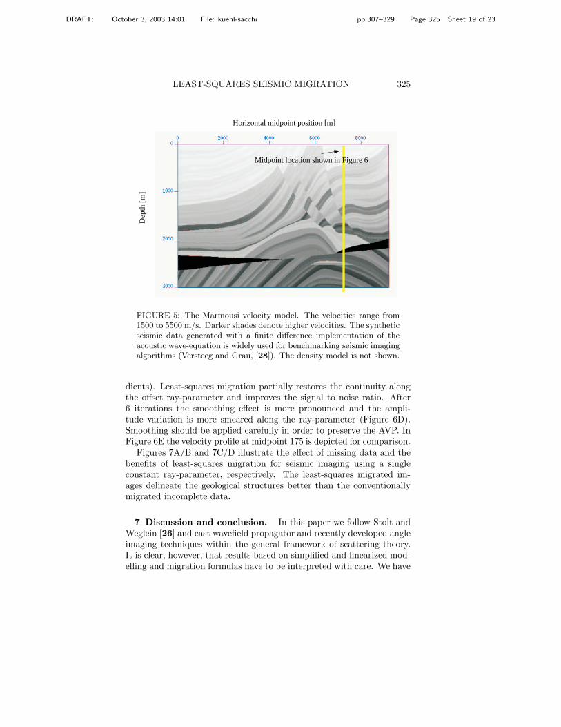
6.1 Synthetic data example. We illustrate least-squares AVP imag-ing with ray-parameter smoothing using the Marmousi data set (Ver-steeg and Grau, [28]). The synthetic Marmousi data are based on avariable velocity (Figure 5) and density model (not shown). Since thedata were modelled with the acoustic wave equation, the angle depen-dence of the reflectors corresponds to the AVA/AVP of a fluid-fluid in-terface.

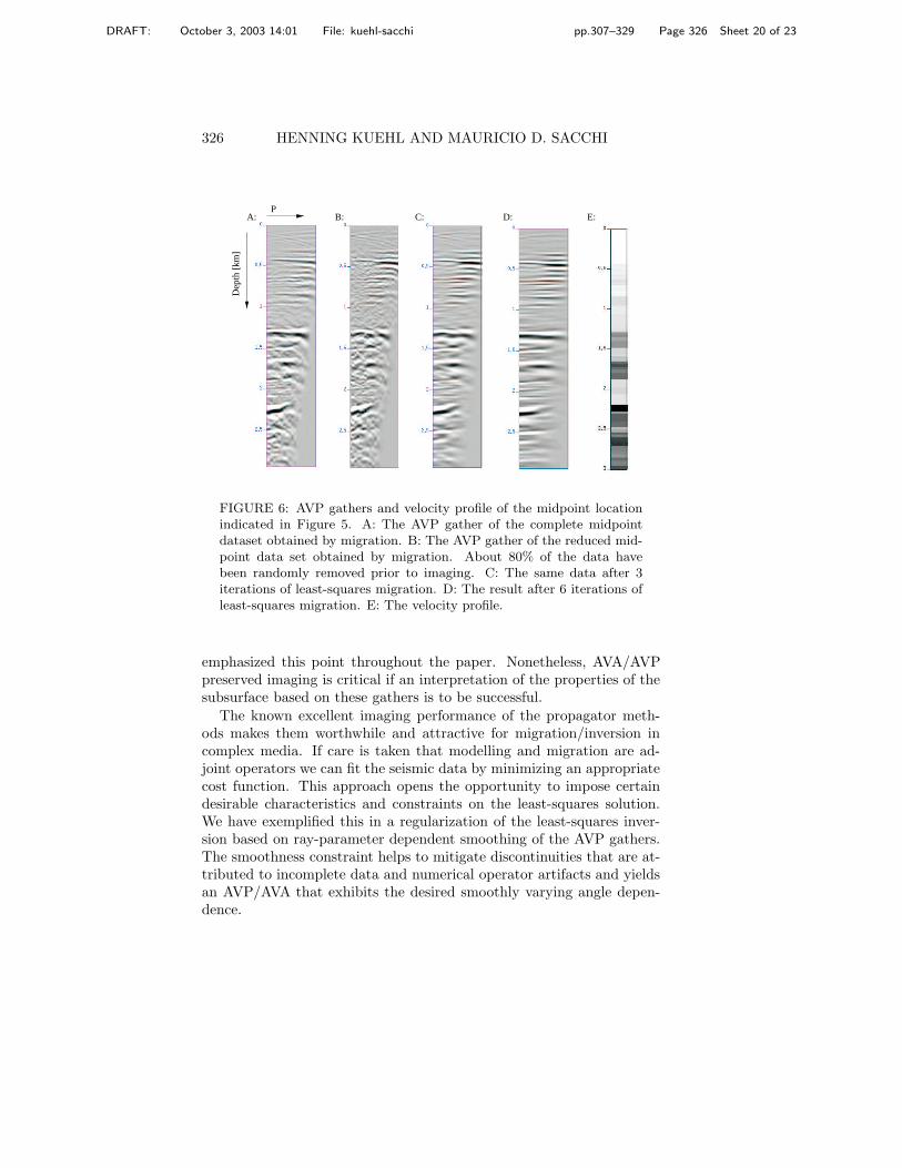
Figure 6A is the AVP gather at midpoint 175 out of a total of 240midpoint positions (see also Figure 5). To generate the gathers the mi-gration operator in equation (33) was applied to the regularly sampleddata set. The gathers were produced with offset ray-parameters rang-ing from 0 to 760 µs/m. AVP effects and numerical imaging artifactsare apparent. We have previously shown for selected reflection eventsthat the retrieved AVA/AVP matches the theoretical AVA/AVP closely(Kuehl and Sacchi, [17]).

To test the influence of missing data on the imaging result we ran-domly replaced 80% of the data with dead traces prior to migration.Figure 6B shows the resulting AVP gathers. They exhibit stronger in-coherent noise and the continuity along the ray-parameter axis is de-teriorated. The effect of least-squares migration with moderate ray-parameter smoothing is demonstrated in Figure 6C. This result wasobtained after 3 iterations of the minimization algorithm (conjugate gra-



Dep

th [

m]

Horizontal midpoint position [m]

Midpoint location shown in Figure 6

FIGURE 5: The Marmousi velocity model. The velocities range from1500 to 5500 m/s. Darker shades denote higher velocities. The syntheticseismic data generated with a finite difference implementation of theacoustic wave-equation is widely used for benchmarking seismic imagingalgorithms (Versteeg and Grau, [28]). The density model is not shown.

dients). Least-squares migration partially restores the continuity alongthe offset ray-parameter and improves the signal to noise ratio. After6 iterations the smoothing effect is more pronounced and the ampli-tude variation is more smeared along the ray-parameter (Figure 6D).Smoothing should be applied carefully in order to preserve the AVP. InFigure 6E the velocity profile at midpoint 175 is depicted for comparison.

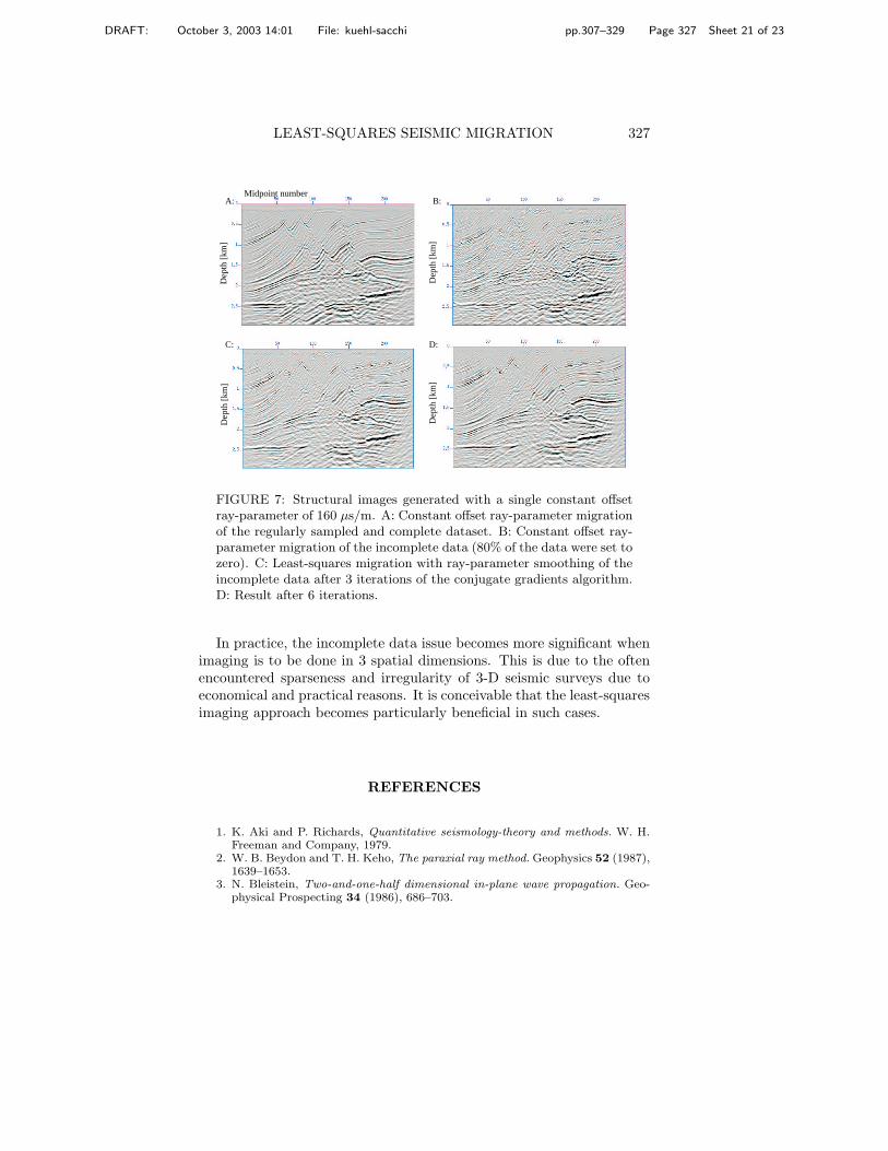
Figures 7A/B and 7C/D illustrate the effect of missing data and thebenefits of least-squares migration for seismic imaging using a singleconstant ray-parameter, respectively. The least-squares migrated im-ages delineate the geological structures better than the conventionallymigrated incomplete data.

7 Discussion and conclusion. In this paper we follow Stolt andWeglein [26] and cast wavefield propagator and recently developed angleimaging techniques within the general framework of scattering theory.It is clear, however, that results based on simplified and linearized mod-elling and migration formulas have to be interpreted with care. We have



p

D

e

p

t

h

[km]

A: B: C: D: E:D

epth

[km

]

PA: B: C: D: E:

FIGURE 6: AVP gathers and velocity profile of the midpoint locationindicated in Figure 5. A: The AVP gather of the complete midpointdataset obtained by migration. B: The AVP gather of the reduced mid-point data set obtained by migration. About 80% of the data havebeen randomly removed prior to imaging. C: The same data after 3iterations of least-squares migration. D: The result after 6 iterations ofleast-squares migration. E: The velocity profile.

emphasized this point throughout the paper. Nonetheless, AVA/AVPpreserved imaging is critical if an interpretation of the properties of thesubsurface based on these gathers is to be successful.

The known excellent imaging performance of the propagator meth-ods makes them worthwhile and attractive for migration/inversion incomplex media. If care is taken that modelling and migration are ad-joint operators we can fit the seismic data by minimizing an appropriatecost function. This approach opens the opportunity to impose certaindesirable characteristics and constraints on the least-squares solution.We have exemplified this in a regularization of the least-squares inver-sion based on ray-parameter dependent smoothing of the AVP gathers.The smoothness constraint helps to mitigate discontinuities that are at-tributed to incomplete data and numerical operator artifacts and yieldsan AVP/AVA that exhibits the desired smoothly varying angle depen-dence.



C:

A: B:

D:

Midpoint number

Dep

th [

km]

Dep

th [

km]

Dep

th [

km]

Dep

th [

km]

FIGURE 7: Structural images generated with a single constant offsetray-parameter of 160 µs/m. A: Constant offset ray-parameter migrationof the regularly sampled and complete dataset. B: Constant offset ray-parameter migration of the incomplete data (80% of the data were set tozero). C: Least-squares migration with ray-parameter smoothing of theincomplete data after 3 iterations of the conjugate gradients algorithm.D: Result after 6 iterations.

In practice, the incomplete data issue becomes more significant whenimaging is to be done in 3 spatial dimensions. This is due to the oftenencountered sparseness and irregularity of 3-D seismic surveys due toeconomical and practical reasons. It is conceivable that the least-squaresimaging approach becomes particularly beneficial in such cases.

REFERENCES

1. K. Aki and P. Richards, Quantitative seismology-theory and methods. W. H.Freeman and Company, 1979.

2. W. B. Beydon and T. H. Keho, The paraxial ray method. Geophysics 52 (1987),1639–1653.

3. N. Bleistein, Two-and-one-half dimensional in-plane wave propagation. Geo-physical Prospecting 34 (1986), 686–703.



4. N. Bleistein, J. K. Cohen and J. W. Stockwell, Mathematics of multidimen-sional seismic imaging, migration, and inversion. Springer-Verlag, 2001.

5. J. F. Claerbout, 1992, Earth Soundings Analysis - Processing versus Inversion.Blackwell Scientific Publications, 1992.

6. R. W. Clayton and R. H. Stolt, A Born-WKBJ inversion method for acousticreflection data. Geophysics 46 (1981), 1559–1567.

7. C. G. M. de Bruin, C. P. A. Wapenaar and A. J. Berkhout, Angle dependentreflectivity by means of prestack migration. Geophysics 55 (1990), 1223–1234.

8. B. Duquet, J. K. Marfurt and J. A. Dellinger, Kirchhoff modeling, inversionfor reflectivity, and subsurface illumination. Geophysics 65 (2000), 1195–1209.

9. J. Gazdag, Wave equation migration with the phase shift method. Geophysics43 (1978), 1342–1351.

10. J. Gazdag and P. Sguazzero, Migration of seismic data by phase shift plusinterpolation. Geophysics 49 (1984), 124–131.

11. S. H. Gray and W. P. May, Kirchhoff migration using eikonal equation travel-times. Geophysics 59 (1994), 810–817.

12. M. R. Hestenes and E. Stiefel, Methods of conjugate gradients for solving linearsystems. J. Research Nat. Bur. Standards 49 (1952), 409–436.

13. W. Kessinger, 1992, Extended split-step Fourier migration. In: 62nd Ann.Internat. Mtg., Soc. Expl. Geophys., Expanded Abstracts, 917–920.

14. H. Kuehl and M. D. Sacchi, Split-step WKBJ migration/inversion of incom-plete data. 5th SEGJ International Symposium—Imaging Technology, 2001.

15. , Separable offset least-squares DSR migration of incomplete data.CSEG National Convention, 2001.

16. , Generalized least-squares DSR migration using a common angle imag-ing condition. In: 71th Ann. Internat. Mtg., Soc. Expl. Geophys., ExpandedAbstracts, MIG 5.6, 2001.

17. , Constrained least-squares wave-equation migration for AVP inversion.64th EAGE annual conference, Florence, 2002.

18. G. F. Margrave and R. J. Ferguson, 1999, Wavefield extrapolation by nonsta-tionary phase shift. Geophysics 64 (1999), 1067–1078.

19. C. C. Mosher and D. J. Foster, Common angle imaging conditions for pre-stackdepth migration. In: 70th Ann. Internat. Mtg., Soc. Expl. Geophys., ExpandedAbstracts, MIG 4.4, 2000.

20. T. Nemeth, C. Wu and G. T. Schuster, Least-squares migration of incompletereflection data. Geophysics 64 (1999), 208–221.

21. R. Ottolini and J. F. Claerbout, The migration of common midpoint slantstacks. Geophysics 49 (1984), 237–249.

22. A. M. Popovici, Prestack migration by split-step DSR. Geophysics 61 (1996),1412–1416.

23. M. Prucha, B. Biondi and W. Symes, Angle-domain common image gathers bywave-equation migration. In: 69th Ann. Internat. Mtg., Soc. Expl. Geophys.,Expanded Abstracts, 1999, 824–827.

24. P. Sava, B. Biondi and S. Fomel, Amplitude preserved common image gathersby wave-equation migration. In: 71th Ann. Internat. Mtg., Soc. Expl. Geophys.,Expanded Abstracts, AVO 5.3, 2001.

25. P. L. Stoffa, J. T. Fokkema, R. M. de Luna Freire and W. P. Kessinger, Split-step Fourier migration. Geophysics 55 (1990), 410–421.

26. R. H. Stolt and A. B. Weglein, Migration and inversion of seismic data. Geo-physics 50 (1985), 2458–2472.

27. R. H. Stolt and A. K. Benson, Seismic Migration: Theory and Practice. Geo-physical Press, 1986.

28. R. Versteeg and G. Grau (eds.), The Marmousi experience: Proceedings of the1990 EAGE Workshop. 52nd EAGE Meeting, Eur., Assoc. Expl. Geophys.,1991.



29. C. P. A. Wapenaar, Inversion versus migration: A new perspective to an olddiscussion. Geophysics 61 (1996), 804–814.

30. , Reciprocity properties of one-way propagators. Geophysics 63 (1998),1795–1798.

Department of Physics, University of Alberta, Edmonton, AB, T6G 2J1

least-squares seismic migration using · pdf filedraft: october 3, 2003 14:01 file:...

Documents