learning statistics with jasplearning statistics with jasp: a tutorial for psychology students and...

Learning Statistics with JASP:A Tutorial for Psychology Students and Other Beginners

(Version1

?2)

Danielle NavarroUniversity of New South [email protected]

David FoxcroftOxford Brookes University

[email protected]

Thomas J. FaulkenberryTarleton State University

[email protected]

http://www.learnstatswithjasp.com

[email protected]

[email protected]

[email protected]

http://www.learnstatswithjasp.com

Overview

Learning Statistics with JASP covers the contents of an introductory statistics class, as typically taughtto undergraduate psychology students. The book discusses how to get started in JASP as well as givingan introduction to data manipulation. From a statistical perspective, the book discusses descriptivestatistics and graphing first, followed by chapters on probability theory, sampling and estimation, andnull hypothesis testing. After introducing the theory, the book covers the analysis of contingencytables, correlation, t-tests, regression, ANOVA and factor analysis. Bayesian statistics is covered atthe end of the book.

Citation

Navarro, D.J., Foxcroft, D.R., & Faulkenberry, T.J. (2019). Learning Statistics with JASP: A Tutorialfor Psychology Students and Other Beginners. (Version 1?

2).

ii

This book is published under a Creative Commons BY-SA license (CC BY-SA) version 4.0. Thismeans that this book can be reused, remixed, retained, revised and redistributed (including

commercially) as long as appropriate credit is given to the authors. If you remix, or modify theoriginal version of this open textbook, you must redistribute all versions of this open textbook under

the same license - CC BY-SA.

https://creativecommons.org/licenses/by-sa/4.0/

iii

https://creativecommons.org/licenses/by-sa/4.0/

The JASP-specific revisions to the original book by Navarro and Foxcroft were madepossible by a generous grant to Tom Faulkenberry from the Tarleton State University

Center for Instructional Innovation.

iv

Table of Contents

Preface ix

I Background 1

1 Why do we learn statistics? 31.1 On the psychology of statistics . . . . . . . . . . . . . . . . . . . . . . . . . . . . . 31.2 The cautionary tale of Simpson’s paradox . . . . . . . . . . . . . . . . . . . . . . . 61.3 Statistics in psychology . . . . . . . . . . . . . . . . . . . . . . . . . . . . . . . . . 91.4 Statistics in everyday life . . . . . . . . . . . . . . . . . . . . . . . . . . . . . . . . 111.5 There’s more to research methods than statistics . . . . . . . . . . . . . . . . . . . 11

2 A brief introduction to research design 132.1 Introduction to psychological measurement . . . . . . . . . . . . . . . . . . . . . . 132.2 Scales of measurement . . . . . . . . . . . . . . . . . . . . . . . . . . . . . . . . . 172.3 Assessing the reliability of a measurement . . . . . . . . . . . . . . . . . . . . . . . 222.4 The “role” of variables: predictors and outcomes . . . . . . . . . . . . . . . . . . . 242.5 Experimental and non-experimental research . . . . . . . . . . . . . . . . . . . . . . 252.6 Assessing the validity of a study . . . . . . . . . . . . . . . . . . . . . . . . . . . . 272.7 Confounds, artefacts and other threats to validity . . . . . . . . . . . . . . . . . . . 302.8 Summary . . . . . . . . . . . . . . . . . . . . . . . . . . . . . . . . . . . . . . . . . 40

II Describing and displaying data with JASP 43

3 Getting started with JASP 453.1 Installing JASP . . . . . . . . . . . . . . . . . . . . . . . . . . . . . . . . . . . . . 463.2 Analyses . . . . . . . . . . . . . . . . . . . . . . . . . . . . . . . . . . . . . . . . . 473.3 Loading data in JASP . . . . . . . . . . . . . . . . . . . . . . . . . . . . . . . . . . 483.4 The spreadsheet . . . . . . . . . . . . . . . . . . . . . . . . . . . . . . . . . . . . . 503.5 Changing data from one measurement scale to another . . . . . . . . . . . . . . . . 523.6 Quitting JASP . . . . . . . . . . . . . . . . . . . . . . . . . . . . . . . . . . . . . 523.7 Summary . . . . . . . . . . . . . . . . . . . . . . . . . . . . . . . . . . . . . . . . . 53

4 Descriptive statistics 554.1 Measures of central tendency . . . . . . . . . . . . . . . . . . . . . . . . . . . . . . 554.2 Measures of variability . . . . . . . . . . . . . . . . . . . . . . . . . . . . . . . . . . 664.3 Skew and kurtosis . . . . . . . . . . . . . . . . . . . . . . . . . . . . . . . . . . . . 734.4 Descriptive statistics separately for each group . . . . . . . . . . . . . . . . . . . . 76

v

4.5 Standard scores . . . . . . . . . . . . . . . . . . . . . . . . . . . . . . . . . . . . . 764.6 Summary . . . . . . . . . . . . . . . . . . . . . . . . . . . . . . . . . . . . . . . . . 78

5 Drawing graphs 835.1 Histograms . . . . . . . . . . . . . . . . . . . . . . . . . . . . . . . . . . . . . . . . 845.2 Boxplots . . . . . . . . . . . . . . . . . . . . . . . . . . . . . . . . . . . . . . . . . 865.3 Saving image files using JASP . . . . . . . . . . . . . . . . . . . . . . . . . . . . . 895.4 Summary . . . . . . . . . . . . . . . . . . . . . . . . . . . . . . . . . . . . . . . . . 90

III Statistical theory 91

6 Introduction to probability 996.1 How are probability and statistics different? . . . . . . . . . . . . . . . . . . . . . . 1006.2 What does probability mean? . . . . . . . . . . . . . . . . . . . . . . . . . . . . . . 1016.3 Basic probability theory . . . . . . . . . . . . . . . . . . . . . . . . . . . . . . . . . 1066.4 The binomial distribution . . . . . . . . . . . . . . . . . . . . . . . . . . . . . . . . 1096.5 The normal distribution . . . . . . . . . . . . . . . . . . . . . . . . . . . . . . . . . 1136.6 Other useful distributions . . . . . . . . . . . . . . . . . . . . . . . . . . . . . . . . 1186.7 Summary . . . . . . . . . . . . . . . . . . . . . . . . . . . . . . . . . . . . . . . . . 122

7 Estimating unknown quantities from a sample 1237.1 Samples, populations and sampling . . . . . . . . . . . . . . . . . . . . . . . . . . . 1237.2 The law of large numbers . . . . . . . . . . . . . . . . . . . . . . . . . . . . . . . . 1317.3 Sampling distributions and the central limit theorem . . . . . . . . . . . . . . . . . 1337.4 Estimating population parameters . . . . . . . . . . . . . . . . . . . . . . . . . . . 1397.5 Estimating a confidence interval . . . . . . . . . . . . . . . . . . . . . . . . . . . . . 1477.6 Summary . . . . . . . . . . . . . . . . . . . . . . . . . . . . . . . . . . . . . . . . . 152

8 Hypothesis testing 1538.1 A menagerie of hypotheses . . . . . . . . . . . . . . . . . . . . . . . . . . . . . . . 1548.2 Two types of errors . . . . . . . . . . . . . . . . . . . . . . . . . . . . . . . . . . . 1578.3 Test statistics and sampling distributions . . . . . . . . . . . . . . . . . . . . . . . 1598.4 Making decisions . . . . . . . . . . . . . . . . . . . . . . . . . . . . . . . . . . . . 1618.5 The p value of a test . . . . . . . . . . . . . . . . . . . . . . . . . . . . . . . . . . 1648.6 Reporting the results of a hypothesis test . . . . . . . . . . . . . . . . . . . . . . . 1678.7 Running the hypothesis test in practice . . . . . . . . . . . . . . . . . . . . . . . . 1698.8 Effect size, sample size and power . . . . . . . . . . . . . . . . . . . . . . . . . . . 1708.9 Some issues to consider . . . . . . . . . . . . . . . . . . . . . . . . . . . . . . . . . 1778.10 Summary . . . . . . . . . . . . . . . . . . . . . . . . . . . . . . . . . . . . . . . . . 179

vi

IV Statistical tools 181

9 Categorical data analysis 1839.1 The χ2 (chi-square) goodness-of-fit test . . . . . . . . . . . . . . . . . . . . . . . . 1839.2 The χ2 test of independence (or association) . . . . . . . . . . . . . . . . . . . . . 1989.3 The continuity correction . . . . . . . . . . . . . . . . . . . . . . . . . . . . . . . . 2039.4 Effect size . . . . . . . . . . . . . . . . . . . . . . . . . . . . . . . . . . . . . . . . 2039.5 Assumptions of the test(s) . . . . . . . . . . . . . . . . . . . . . . . . . . . . . . . 2049.6 Summary . . . . . . . . . . . . . . . . . . . . . . . . . . . . . . . . . . . . . . . . . 205

10 Comparing two means 20710.1 The one-sample z-test . . . . . . . . . . . . . . . . . . . . . . . . . . . . . . . . . . 20810.2 The one-sample t-test . . . . . . . . . . . . . . . . . . . . . . . . . . . . . . . . . 21410.3 The independent samples t-test (Student test) . . . . . . . . . . . . . . . . . . . . 21910.4 The independent samples t-test (Welch test) . . . . . . . . . . . . . . . . . . . . . 22910.5 The paired-samples t-test . . . . . . . . . . . . . . . . . . . . . . . . . . . . . . . 23210.6 One sided tests . . . . . . . . . . . . . . . . . . . . . . . . . . . . . . . . . . . . . 23710.7 Effect size . . . . . . . . . . . . . . . . . . . . . . . . . . . . . . . . . . . . . . . . 23810.8 Checking the normality of a sample . . . . . . . . . . . . . . . . . . . . . . . . . . . 24110.9 Testing non-normal data with Wilcoxon tests . . . . . . . . . . . . . . . . . . . . . . 24610.10 Summary . . . . . . . . . . . . . . . . . . . . . . . . . . . . . . . . . . . . . . . . . 248

11 Correlation and linear regression 25111.1 Correlations . . . . . . . . . . . . . . . . . . . . . . . . . . . . . . . . . . . . . . . 25111.2 Scatterplots . . . . . . . . . . . . . . . . . . . . . . . . . . . . . . . . . . . . . . . 26111.3 What is a linear regression model? . . . . . . . . . . . . . . . . . . . . . . . . . . . 26211.4 Estimating a linear regression model . . . . . . . . . . . . . . . . . . . . . . . . . . 26511.5 Multiple linear regression . . . . . . . . . . . . . . . . . . . . . . . . . . . . . . . . 26711.6 Quantifying the fit of the regression model . . . . . . . . . . . . . . . . . . . . . . 27011.7 Hypothesis tests for regression models . . . . . . . . . . . . . . . . . . . . . . . . . 27311.8 Regarding regression coefficients . . . . . . . . . . . . . . . . . . . . . . . . . . . . 27711.9 Assumptions of regression . . . . . . . . . . . . . . . . . . . . . . . . . . . . . . . 27911.10 Model checking . . . . . . . . . . . . . . . . . . . . . . . . . . . . . . . . . . . . . 28011.11 Model selection . . . . . . . . . . . . . . . . . . . . . . . . . . . . . . . . . . . . . 28811.12 Summary . . . . . . . . . . . . . . . . . . . . . . . . . . . . . . . . . . . . . . . . . 290

12 Comparing several means (one-way ANOVA) 29312.1 An illustrative data set . . . . . . . . . . . . . . . . . . . . . . . . . . . . . . . . . 29312.2 How ANOVA works . . . . . . . . . . . . . . . . . . . . . . . . . . . . . . . . . . . 29512.3 Running an ANOVA in JASP . . . . . . . . . . . . . . . . . . . . . . . . . . . . . . 30512.4 Effect size . . . . . . . . . . . . . . . . . . . . . . . . . . . . . . . . . . . . . . . . 30612.5 Multiple comparisons and post hoc tests . . . . . . . . . . . . . . . . . . . . . . . . 30712.6 Assumptions of one-way ANOVA . . . . . . . . . . . . . . . . . . . . . . . . . . . . 311

vii

12.7 Removing the normality assumption . . . . . . . . . . . . . . . . . . . . . . . . . . 31512.8 Repeated measures one-way ANOVA . . . . . . . . . . . . . . . . . . . . . . . . . . 31912.9 The Friedman non-parametric repeated measures ANOVA test . . . . . . . . . . . . 32412.10 On the relationship between ANOVA and the Student t-test . . . . . . . . . . . . . 32512.11 Summary . . . . . . . . . . . . . . . . . . . . . . . . . . . . . . . . . . . . . . . . . 325

13 Factorial ANOVA 32713.1 Factorial ANOVA 1: balanced designs, no interactions . . . . . . . . . . . . . . . . . 32713.2 Factorial ANOVA 2: balanced designs, interactions allowed . . . . . . . . . . . . . . 33913.3 Effect size . . . . . . . . . . . . . . . . . . . . . . . . . . . . . . . . . . . . . . . . 34613.4 Assumption checking . . . . . . . . . . . . . . . . . . . . . . . . . . . . . . . . . . 34913.5 Analysis of Covariance (ANCOVA) . . . . . . . . . . . . . . . . . . . . . . . . . . . 35113.6 ANOVA as a linear model . . . . . . . . . . . . . . . . . . . . . . . . . . . . . . . . 35313.7 Different ways to specify contrasts . . . . . . . . . . . . . . . . . . . . . . . . . . . 36113.8 Post hoc tests . . . . . . . . . . . . . . . . . . . . . . . . . . . . . . . . . . . . . . 36513.9 The method of planned comparisons . . . . . . . . . . . . . . . . . . . . . . . . . . 36813.10 Factorial ANOVA 3: unbalanced designs . . . . . . . . . . . . . . . . . . . . . . . . 36913.11 Summary . . . . . . . . . . . . . . . . . . . . . . . . . . . . . . . . . . . . . . . . . 380

V Endings, alternatives and prospects 381

14 Bayesian statistics 38314.1 Probabilistic reasoning by rational agents . . . . . . . . . . . . . . . . . . . . . . . . 38414.2 Bayesian hypothesis tests . . . . . . . . . . . . . . . . . . . . . . . . . . . . . . . . 38914.3 Why be a Bayesian? . . . . . . . . . . . . . . . . . . . . . . . . . . . . . . . . . . . 39114.4 Bayesian t-tests . . . . . . . . . . . . . . . . . . . . . . . . . . . . . . . . . . . . . 39914.5 Summary . . . . . . . . . . . . . . . . . . . . . . . . . . . . . . . . . . . . . . . . . 401

15 Epilogue 40315.1 The undiscovered statistics . . . . . . . . . . . . . . . . . . . . . . . . . . . . . . . 40315.2 Learning the basics, and learning them in JASP . . . . . . . . . . . . . . . . . . . . 411

16 References 415

viii

Preface to Version 1{?

2

I am happy to introduce “Learning Statistics with JASP”, an adaptation of the excellent “Learningstatistics with jamovi” and “Learning Statistics with R”. This version builds on the wonderful previouswork of Dani Navarro and David Foxcroft, without whose previous efforts a book of this quality wouldnot be possible. I had a simple aim when I begain working on this adaption: I wanted to use theNavarro and Foxcroft text in my own statistics courses, but for reasons I won’t get into right now, Iuse JASP instead of jamovi. Both are wonderful tools, but I have a not-so-slight tendency to preferJASP, possibly because I was using JASP before jamovi split off as a separate project. Nonetheless, Iam happy to help bring this book into the world for JASP users.

I am grateful to the Center for Instructional Innovation at Tarleton State University, who gave mea grant to pursue the writing of this open educational resource (OER) in Summer 2019. I am lookingforward to providing my future students (and students everywhere) with a quality statistics text thatis (and forever shall be) 100% free!

I invite readers everywhere to find ways to make this text better (including identiying the ever-present typos). Please send me an email if you’d like to contribute (or feel free to go to my Githubpage and just fork it yourself. Go crazy!

Thomas J. FaulkenberryJuly 12, 2019

Preface to Version 0.70

This update from version 0.65 introduces some new analyses. In the ANOVA chapters we have addedsections on repeated measures ANOVA and analysis of covariance (ANCOVA). In a new chapter wehave introduced Factor Analysis and related techniques. Hopefully the style of this new material isconsistent with the rest of the book, though eagle-eyed readers might spot a bit more of an emphasison conceptual and practical explanations, and a bit less algebra. I’m not sure this is a good thing, andmight add the algebra in a bit later. But it reflects both my approach to understanding and teachingstatistics, and also some feedback I have received from students on a course I teach. In line with this,I have also been through the rest of the book and tried to separate out some of the algebra by puttingit into a box or frame. It’s not that this stuff is not important or useful, but for some students theymay wish to skip over it and therefore the boxing of these parts should help some readers.

With this version I am very grateful to comments and feedback received from my students andcolleagues, notably Wakefield Morys-Carter, and also to numerous people all over the world who havesent in small suggestions and corrections - much appreciated, and keep them coming! One pretty neatnew feature is that the example data files for the book can now be loaded into jamovi as an add-onmodule - thanks to Jonathon Love for helping with that.

David Foxcroft

ix

February 1st, 2019


In this adaptation of the excellent ‘Learning statistics with R’, by Danielle Navarro, we have replacedthe statistical software used for the analyses and examples with jamovi. Although R is a powerfulstatistical programming language, it is not the first choice for every instructor and student at thebeginning of their statistical learning. Some instructors and students tend to prefer the point-and-click style of software, and that’s where jamovi comes in. jamovi is software that aims to simplifytwo aspects of using R. It offers a point-and-click graphical user interface (GUI), and it also providesfunctions that combine the capabilities of many others, bringing a more SPSS- or SAS-like method ofprogramming to R. Importantly, jamovi will always be free and open - that’s one of its core values -because jamovi is made by the scientific community, for the scientific community.

With this version I am very grateful for the help of others who have read through drafts andprovided excellent suggestions and corrections, particularly Dr David Emery and Kirsty Walter.

David FoxcroftJuly 1st, 2018


The book hasn’t changed much since 2015 when I released Version 0.5 – it’s probably fair to say thatI’ve changed more than it has. I moved from Adelaide to Sydney in 2016 and my teaching profile atUNSW is different to what it was at Adelaide, and I haven’t really had a chance to work on it sincearriving here! It’s a little strange looking back at this actually. A few quick comments...

• Weirdly, the book consistently misgenders me, but I suppose I have only myself to blame for thatone :-) There’s now a brief footnote on page 12 that mentions this issue; in real life I’ve beenworking through a gender affirmation process for the last two years and mostly go by she/herpronouns. I am, however, just as lazy as I ever was so I haven’t bothered updating the text inthe book.

• For Version 0.6 I haven’t changed much I’ve made a few minor changes when people havepointed out typos or other errors. In particular it’s worth noting the issue associated with theetaSquared function in the lsr package (which isn’t really being maintained any more) in Section14.4. The function works fine for the simple examples in the book, but there are definitely bugsin there that I haven’t found time to check! So please take care with that one.

x

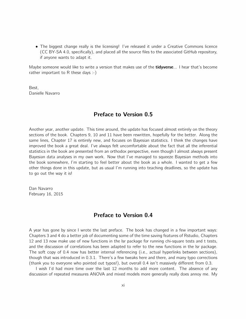
• The biggest change really is the licensing! I’ve released it under a Creative Commons licence(CC BY-SA 4.0, specifically), and placed all the source files to the associated GitHub repository,if anyone wants to adapt it.

Maybe someone would like to write a version that makes use of the tidyverse... I hear that’s becomerather important to R these days :-)

Best,Danielle Navarro


Another year, another update. This time around, the update has focused almost entirely on the theorysections of the book. Chapters 9, 10 and 11 have been rewritten, hopefully for the better. Along thesame lines, Chapter 17 is entirely new, and focuses on Bayesian statistics. I think the changes haveimproved the book a great deal. I’ve always felt uncomfortable about the fact that all the inferentialstatistics in the book are presented from an orthodox perspective, even though I almost always presentBayesian data analyses in my own work. Now that I’ve managed to squeeze Bayesian methods intothe book somewhere, I’m starting to feel better about the book as a whole. I wanted to get a fewother things done in this update, but as usual I’m running into teaching deadlines, so the update hasto go out the way it is!

Dan NavarroFebruary 16, 2015


A year has gone by since I wrote the last preface. The book has changed in a few important ways:Chapters 3 and 4 do a better job of documenting some of the time saving features of Rstudio, Chapters12 and 13 now make use of new functions in the lsr package for running chi-square tests and t tests,and the discussion of correlations has been adapted to refer to the new functions in the lsr package.The soft copy of 0.4 now has better internal referencing (i.e., actual hyperlinks between sections),though that was introduced in 0.3.1. There’s a few tweaks here and there, and many typo corrections(thank you to everyone who pointed out typos!), but overall 0.4 isn’t massively different from 0.3.

I wish I’d had more time over the last 12 months to add more content. The absence of anydiscussion of repeated measures ANOVA and mixed models more generally really does annoy me. My

xi

excuse for this lack of progress is that my second child was born at the start of 2013, and so I spentmost of last year just trying to keep my head above water. As a consequence, unpaid side projectslike this book got sidelined in favour of things that actually pay my salary! Things are a little calmernow, so with any luck version 0.5 will be a bigger step forward.

One thing that has surprised me is the number of downloads the book gets. I finally got some basictracking information from the website a couple of months ago, and (after excluding obvious robots)the book has been averaging about 90 downloads per day. That’s encouraging: there’s at least a fewpeople who find the book useful!

Dan NavarroFebruary 4, 2014


There’s a part of me that really doesn’t want to publish this book. It’s not finished.

And when I say that, I mean it. The referencing is spotty at best, the chapter summaries arejust lists of section titles, there’s no index, there are no exercises for the reader, the organisation issuboptimal, and the coverage of topics is just not comprehensive enough for my liking. Additionally,there are sections with content that I’m not happy with, figures that really need to be redrawn, andI’ve had almost no time to hunt down inconsistencies, typos, or errors. In other words, this book is notfinished. If I didn’t have a looming teaching deadline and a baby due in a few weeks, I really wouldn’tbe making this available at all.

What this means is that if you are an academic looking for teaching materials, a Ph.D. studentlooking to learn R, or just a member of the general public interested in statistics, I would advise youto be cautious. What you’re looking at is a first draft, and it may not serve your purposes. If wewere living in the days when publishing was expensive and the internet wasn’t around, I would neverconsider releasing a book in this form. The thought of someone shelling out $80 for this (which iswhat a commercial publisher told me it would retail for when they offered to distribute it) makes mefeel more than a little uncomfortable. However, it’s the 21st century, so I can post the pdf on mywebsite for free, and I can distribute hard copies via a print-on-demand service for less than half whata textbook publisher would charge. And so my guilt is assuaged, and I’m willing to share! With thatin mind, you can obtain free soft copies and cheap hard copies online, from the following webpages:

Soft copy: http://www.compcogscisydney.com/learning-statistics-with-r.htmlHard copy: www.lulu.com/content/13570633

Even so, the warning still stands: what you are looking at is Version 0.3 of a work in progress.If and when it hits Version 1.0, I would be willing to stand behind the work and say, yes, this is atextbook that I would encourage other people to use. At that point, I’ll probably start shamelessly

xii

http://www.compcogscisydney.com/learning-statistics-with-r.html

www.lulu.com/content/13570633

flogging the thing on the internet and generally acting like a tool. But until that day comes, I’d likeit to be made clear that I’m really ambivalent about the work as it stands.

All of the above being said, there is one group of people that I can enthusiastically endorse thisbook to: the psychology students taking our undergraduate research methods classes (DRIP andDRIP:A) in 2013. For you, this book is ideal, because it was written to accompany your stats lectures.If a problem arises due to a shortcoming of these notes, I can and will adapt content on the fly tofix that problem. Effectively, you’ve got a textbook written specifically for your classes, distributedfor free (electronic copy) or at near-cost prices (hard copy). Better yet, the notes have been tested:Version 0.1 of these notes was used in the 2011 class, Version 0.2 was used in the 2012 class, and nowyou’re looking at the new and improved Version 0.3. I’[for a historical summary]m not saying thesenotes are titanium plated awesomeness on a stick – though if you wanted to say so on the studentevaluation forms, then you’re totally welcome to – because they’re not. But I am saying that they’vebeen tried out in previous years and they seem to work okay. Besides, there’s a group of us around totroubleshoot if any problems come up, and you can guarantee that at least one of your lecturers hasread the whole thing cover to cover!

Okay, with all that out of the way, I should say something about what the book aims to be. Atits core, it is an introductory statistics textbook pitched primarily at psychology students. As such,it covers the standard topics that you’d expect of such a book: study design, descriptive statistics,the theory of hypothesis testing, t-tests, χ2 tests, ANOVA and regression. However, there are alsoseveral chapters devoted to the R statistical package, including a chapter on data manipulation andanother one on scripts and programming. Moreover, when you look at the content presented in thebook, you’ll notice a lot of topics that are traditionally swept under the carpet when teaching statisticsto psychology students. The Bayesian/frequentist divide is openly disussed in the probability chapter,and the disagreement between Neyman and Fisher about hypothesis testing makes an appearance.The difference between probability and density is discussed. A detailed treatment of Type I, II and IIIsums of squares for unbalanced factorial ANOVA is provided. And if you have a look in the Epilogue,it should be clear that my intention is to add a lot more advanced content.

My reasons for pursuing this approach are pretty simple: the students can handle it, and they evenseem to enjoy it. Over the last few years I’ve been pleasantly surprised at just how little difficulty I’vehad in getting undergraduate psych students to learn R. It’s certainly not easy for them, and I’ve foundI need to be a little charitable in setting marking standards, but they do eventually get there. Similarly,they don’t seem to have a lot of problems tolerating ambiguity and complexity in presentation ofstatistical ideas, as long as they are assured that the assessment standards will be set in a fashion thatis appropriate for them. So if the students can handle it, why not teach it? The potential gains arepretty enticing. If they learn R, the students get access to CRAN, which is perhaps the largest andmost comprehensive library of statistical tools in existence. And if they learn about probability theoryin detail, it’s easier for them to switch from orthodox null hypothesis testing to Bayesian methods ifthey want to. Better yet, they learn data analysis skills that they can take to an employer withoutbeing dependent on expensive and proprietary software.

Sadly, this book isn’t the silver bullet that makes all this possible. It’s a work in progress, and

xiii

maybe when it is finished it will be a useful tool. One among many, I would think. There are a numberof other books that try to provide a basic introduction to statistics using R, and I’m not arrogantenough to believe that mine is better. Still, I rather like the book, and maybe other people will find ituseful, incomplete though it is.

Dan NavarroJanuary 13, 2013

xiv

Part I.

Background

- 1 -

1. Why do we learn statistics?

“Thou shalt not answer questionnairesOr quizzes upon World Affairs,

Nor with complianceTake any test. Thou shalt not sitWith statisticians nor commit

A social science"

– W.H. Auden1

1.1

On the psychology of statistics

To the surprise of many students, statistics is a fairly significant part of a psychological education.To the surprise of no-one, statistics is very rarely the favourite part of one’s psychological education.After all, if you really loved the idea of doing statistics, you’d probably be enrolled in a statistics classright now, not a psychology class. So, not surprisingly, there’s a pretty large proportion of the studentbase that isn’t happy about the fact that psychology has so much statistics in it. In view of this, Ithought that the right place to start might be to answer some of the more common questions thatpeople have about stats.

A big part of this issue at hand relates to the very idea of statistics. What is it? What’s it therefor? And why are scientists so bloody obsessed with it? These are all good questions, when you thinkabout it. So let’s start with the last one. As a group, scientists seem to be bizarrely fixated on runningstatistical tests on everything. In fact, we use statistics so often that we sometimes forget to explainto people why we do. It’s a kind of article of faith among scientists – and especially social scientists

1The quote comes from Auden’s 1946 poem Under Which Lyre: A Reactionary Tract for the Times, deliveredas part of a commencement address at Harvard University. The history of the poem is kind of interesting: http://harvardmagazine.com/2007/11/a-poets-warning.html

- 3 -

http://harvardmagazine.com/2007/11/a-poets-warning.html

http://harvardmagazine.com/2007/11/a-poets-warning.html

– that your findings can’t be trusted until you’ve done some stats. Undergraduate students might beforgiven for thinking that we’re all completely mad, because no-one takes the time to answer one verysimple question:

Why do you do statistics? Why don’t scientists just use common sense?

It’s a naive question in some ways, but most good questions are. There’s a lot of good answers to it,2

but for my money, the best answer is a really simple one: we don’t trust ourselves enough. We worrythat we’re human, and susceptible to all of the biases, temptations and frailties that humans sufferfrom. Much of statistics is basically a safeguard. Using “common sense” to evaluate evidence meanstrusting gut instincts, relying on verbal arguments and on using the raw power of human reason tocome up with the right answer. Most scientists don’t think this approach is likely to work.

In fact, come to think of it, this sounds a lot like a psychological question to me, and since I dowork in a psychology department, it seems like a good idea to dig a little deeper here. Is it reallyplausible to think that this “common sense” approach is very trustworthy? Verbal arguments have tobe constructed in language, and all languages have biases – some things are harder to say than others,and not necessarily because they’re false (e.g., quantum electrodynamics is a good theory, but hardto explain in words). The instincts of our “gut” aren’t designed to solve scientific problems, they’redesigned to handle day to day inferences – and given that biological evolution is slower than culturalchange, we should say that they’re designed to solve the day to day problems for a different world thanthe one we live in. Most fundamentally, reasoning sensibly requires people to engage in “induction”,making wise guesses and going beyond the immediate evidence of the senses to make generalisationsabout the world. If you think that you can do that without being influenced by various distractors,well, I have a bridge in London I’d like to sell you. Heck, as the next section shows, we can’t even solve“deductive” problems (ones where no guessing is required) without being influenced by our pre-existingbiases.

1.1.1 The curse of belief bias

People are mostly pretty smart. We’re certainly smarter than the other species that we sharethe planet with (though many people might disagree). Our minds are quite amazing things, and weseem to be capable of the most incredible feats of thought and reason. That doesn’t make us perfectthough. And among the many things that psychologists have shown over the years is that we reallydo find it hard to be neutral, to evaluate evidence impartially and without being swayed by pre-existingbiases. A good example of this is the belief bias effect in logical reasoning: if you ask people todecide whether a particular argument is logically valid (i.e., conclusion would be true if the premiseswere true), we tend to be influenced by the believability of the conclusion, even when we shouldn’t.For instance, here’s a valid argument where the conclusion is believable:

All cigarettes are expensive (Premise 1)Some addictive things are inexpensive (Premise 2)

2Including the suggestion that common sense is in short supply among scientists.

- 4 -

Therefore, some addictive things are not cigarettes (Conclusion)

And here’s a valid argument where the conclusion is not believable:

All addictive things are expensive (Premise 1)Some cigarettes are inexpensive (Premise 2)Therefore, some cigarettes are not addictive (Conclusion)

The logical structure of argument #2 is identical to the structure of argument #1, and they’re bothvalid. However, in the second argument, there are good reasons to think that premise 1 is incorrect,and as a result it’s probably the case that the conclusion is also incorrect. But that’s entirely irrelevantto the topic at hand; an argument is deductively valid if the conclusion is a logical consequence of thepremises. That is, a valid argument doesn’t have to involve true statements.

On the other hand, here’s an invalid argument that has a believable conclusion:

All addictive things are expensive (Premise 1)Some cigarettes are inexpensive (Premise 2)Therefore, some addictive things are not cigarettes (Conclusion)

And finally, an invalid argument with an unbelievable conclusion:

All cigarettes are expensive (Premise 1)Some addictive things are inexpensive (Premise 2)Therefore, some cigarettes are not addictive (Conclusion)

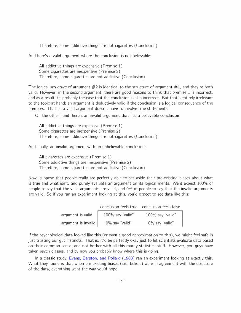
Now, suppose that people really are perfectly able to set aside their pre-existing biases about whatis true and what isn’t, and purely evaluate an argument on its logical merits. We’d expect 100% ofpeople to say that the valid arguments are valid, and 0% of people to say that the invalid argumentsare valid. So if you ran an experiment looking at this, you’d expect to see data like this:

conclusion feels true conclusion feels false

argument is valid 100% say “valid” 100% say “valid”

argument is invalid 0% say “valid” 0% say “valid”

If the psychological data looked like this (or even a good approximation to this), we might feel safe injust trusting our gut instincts. That is, it’d be perfectly okay just to let scientists evaluate data basedon their common sense, and not bother with all this murky statistics stuff. However, you guys havetaken psych classes, and by now you probably know where this is going.

In a classic study, Evans, Barston, and Pollard (1983) ran an experiment looking at exactly this.What they found is that when pre-existing biases (i.e., beliefs) were in agreement with the structureof the data, everything went the way you’d hope:

- 5 -


argument is valid 92% say “valid”

argument is invalid 8% say “valid”

Not perfect, but that’s pretty good. But look what happens when our intuitive feelings about thetruth of the conclusion run against the logical structure of the argument:


argument is valid 92% say “valid” 46% say “valid”

argument is invalid 92% say “valid” 8% say “valid”

Oh dear, that’s not as good. Apparently, when people are presented with a strong argument thatcontradicts our pre-existing beliefs, we find it pretty hard to even perceive it to be a strong argument(people only did so 46% of the time). Even worse, when people are presented with a weak argumentthat agrees with our pre-existing biases, almost no-one can see that the argument is weak (people gotthat one wrong 92% of the time!).3

If you think about it, it’s not as if these data are horribly damning. Overall, people did do betterthan chance at compensating for their prior biases, since about 60% of people’s judgements werecorrect (you’d expect 50% by chance). Even so, if you were a professional “evaluator of evidence”,and someone came along and offered you a magic tool that improves your chances of making the rightdecision from 60% to (say) 95%, you’d probably jump at it, right? Of course you would. Thankfully,we actually do have a tool that can do this. But it’s not magic, it’s statistics. So that’s reason #1why scientists love statistics. It’s just too easy for us to “believe what we want to believe”. So instead,if we want to “believe in the data”, we’re going to need a bit of help to keep our personal biases undercontrol. That’s what statistics does, it helps keep us honest.

1.2

The cautionary tale of Simpson’s paradox

The following is a true story (I think!). In 1973, the University of California, Berkeley had some worriesabout the admissions of students into their postgraduate courses. Specifically, the thing that causedthe problem was that the gender breakdown of their admissions, which looked like this:

Number of applicants Percent admittedMales 8442 44%Females 4321 35%

3In my more cynical moments I feel like this fact alone explains 95% of what I read on the internet.

- 6 -

Given this, they were worried about being sued!4 Given that there were nearly 13,000 applicants, adifference of 9% in admission rates between males and females is just way too big to be a coincidence.Pretty compelling data, right? And if I were to say to you that these data actually reflect a weak biasin favour of women (sort of!), you’d probably think that I was either crazy or sexist.

Oddly, it’s actually sort of true. When people started looking more carefully at the admissionsdata they told a rather different story (Bickel, Hammel, and O’Connell 1975). Specifically, whenthey looked at it on a department by department basis, it turned out that most of the departmentsactually had a slightly higher success rate for female applicants than for male applicants. The tablebelow shows the admission figures for the six largest departments (with the names of the departmentsremoved for privacy reasons):

Males FemalesDepartment Applicants Percent admitted Applicants Percent admitted

A 825 62% 108 82%B 560 63% 25 68%C 325 37% 593 34%D 417 33% 375 35%E 191 28% 393 24%F 272 6% 341 7%

Remarkably, most departments had a higher rate of admissions for females than for males! Yet theoverall rate of admission across the university for females was lower than for males. How can this be?How can both of these statements be true at the same time?

Here’s what’s going on. Firstly, notice that the departments are not equal to one another in termsof their admission percentages: some departments (e.g., A, B) tended to admit a high percentageof the qualified applicants, whereas others (e.g., F) tended to reject most of the candidates, evenif they were high quality. So, among the six departments shown above, notice that department A isthe most generous, followed by B, C, D, E and F in that order. Next, notice that males and femalestended to apply to different departments. If we rank the departments in terms of the total number ofmale applicants, we get AąBąDąCąFąE (the “easy” departments are in bold). On the whole, malestended to apply to the departments that had high admission rates. Now compare this to how thefemale applicants distributed themselves. Ranking the departments in terms of the total number offemale applicants produces a quite different ordering CąEąDąFąAąB. In other words, what thesedata seem to be suggesting is that the female applicants tended to apply to “harder” departments.And in fact, if we look at Figure 1.1 we see that this trend is systematic, and quite striking. Thiseffect is known as Simpson’s paradox. It’s not common, but it does happen in real life, and mostpeople are very surprised by it when they first encounter it, and many people refuse to even believethat it’s real. It is very real. And while there are lots of very subtle statistical lessons buried in there,I want to use it to make a much more important point: doing research is hard, and there are lots

4Earlier versions of these notes incorrectly suggested that they actually were sued. But that’s not true. There’s anice commentary on this here: https://www.refsmmat.com/posts/2016-05-08-simpsons-paradox-berkeley.html.A big thank you to Wilfried Van Hirtum for pointing this out to me.

- 7 -

https://www.refsmmat.com/posts/2016-05-08-simpsons-paradox-berkeley.html

0 20 40 60 80 100

02

04

06

08

01

00

Percentage of female applicants

Ad

mis

sio

n r

ate

(b

oth

ge

nd

ers

)

Figure 1.1: The Berkeley 1973 college admissions data. This figure plots the admission rate for the85 departments that had at least one female applicant, as a function of the percentage of applicantsthat were female. The plot is a redrawing of Figure 1 from Bickel, Hammel, and O’Connell (1975).Circles plot departments with more than 40 applicants; the area of the circle is proportional to thetotal number of applicants. The crosses plot departments with fewer than 40 applicants.

. . . . . . . . . . . . . . . . . . . . . . . . . . . . . . . . . . . . . . . . . . . . . . . . . . . . . . . . . . . . . . . . . . . . . . . . . . . . . . . . . . . . . . . . . . . .

of subtle, counter-intuitive traps lying in wait for the unwary. That’s reason #2 why scientists lovestatistics, and why we teach research methods. Because science is hard, and the truth is sometimescunningly hidden in the nooks and crannies of complicated data.

Before leaving this topic entirely, I want to point out something else really critical that is oftenoverlooked in a research methods class. Statistics only solves part of the problem. Remember thatwe started all this with the concern that Berkeley’s admissions processes might be unfairly biasedagainst female applicants. When we looked at the “aggregated” data, it did seem like the universitywas discriminating against women, but when we “disaggregate” and looked at the individual behaviourof all the departments, it turned out that the actual departments were, if anything, slightly biased in

- 8 -

favour of women. The gender bias in total admissions was caused by the fact that women tended toself-select for harder departments. From a legal perspective, that would probably put the universityin the clear. Postgraduate admissions are determined at the level of the individual department, andthere are good reasons to do that. At the level of individual departments the decisions are more orless unbiased (the weak bias in favour of females at that level is small, and not consistent acrossdepartments). Since the university can’t dictate which departments people choose to apply to, andthe decision making takes place at the level of the department it can hardly be held accountable forany biases that those choices produce.

That was the basis for my somewhat glib remarks earlier, but that’s not exactly the whole story,is it? After all, if we’re interested in this from a more sociological and psychological perspective, wemight want to ask why there are such strong gender differences in applications. Why do males tendto apply to engineering more often than females, and why is this reversed for the English department?And why is it the case that the departments that tend to have a female-application bias tend to havelower overall admission rates than those departments that have a male-application bias? Might this notstill reflect a gender bias, even though every single department is itself unbiased? It might. Suppose,hypothetically, that males preferred to apply to “hard sciences” and females prefer “humanities”. Andsuppose further that the reason for why the humanities departments have low admission rates isbecause the government doesn’t want to fund the humanities (Ph.D. places, for instance, are oftentied to government funded research projects). Does that constitute a gender bias? Or just anunenlightened view of the value of the humanities? What if someone at a high level in the governmentcut the humanities funds because they felt that the humanities are “useless chick stuff”. That seemspretty blatantly gender biased. None of this falls within the purview of statistics, but it matters tothe research project. If you’re interested in the overall structural effects of subtle gender biases, thenyou probably want to look at both the aggregated and disaggregated data. If you’re interested in thedecision making process at Berkeley itself then you’re probably only interested in the disaggregateddata.

In short there are a lot of critical questions that you can’t answer with statistics, but the answersto those questions will have a huge impact on how you analyse and interpret data. And this is thereason why you should always think of statistics as a tool to help you learn about your data. No moreand no less. It’s a powerful tool to that end, but there’s no substitute for careful thought.

1.3

Statistics in psychology

I hope that the discussion above helped explain why science in general is so focused on statistics. ButI’m guessing that you have a lot more questions about what role statistics plays in psychology, andspecifically why psychology classes always devote so many lectures to stats. So here’s my attempt toanswer a few of them...

- 9 -

• Why does psychology have so much statistics?

To be perfectly honest, there’s a few different reasons, some of which are better than others.The most important reason is that psychology is a statistical science. What I mean by thatis that the “things” that we study are people. Real, complicated, gloriously messy, infuriatinglyperverse people. The “things” of physics include objects like electrons, and while there are allsorts of complexities that arise in physics, electrons don’t have minds of their own. They don’thave opinions, they don’t differ from each other in weird and arbitrary ways, they don’t getbored in the middle of an experiment, and they don’t get angry at the experimenter and thendeliberately try to sabotage the data set (not that I’ve ever done that!). At a fundamental levelpsychology is harder than physics.5

Basically, we teach statistics to you as psychologists because you need to be better at statsthan physicists. There’s actually a saying used sometimes in physics, to the effect that “if yourexperiment needs statistics, you should have done a better experiment". They have the luxuryof being able to say that because their objects of study are pathetically simple in comparison tothe vast mess that confronts social scientists. And it’s not just psychology. Most social sciencesare desperately reliant on statistics. Not because we’re bad experimenters, but because we’vepicked a harder problem to solve. We teach you stats because you really, really need it.

• Can’t someone else do the statistics?

To some extent, but not completely. It’s true that you don’t need to become a fully trainedstatistician just to do psychology, but you do need to reach a certain level of statistical compe-tence. In my view, there’s three reasons that every psychological researcher ought to be able todo basic statistics:

– Firstly, there’s the fundamental reason: statistics is deeply intertwined with research design.If you want to be good at designing psychological studies, you need to at the very leastunderstand the basics of stats.

– Secondly, if you want to be good at the psychological side of the research, then you needto be able to understand the psychological literature, right? But almost every paper in thepsychological literature reports the results of statistical analyses. So if you really want tounderstand the psychology, you need to be able to understand what other people did withtheir data. And that means understanding a certain amount of statistics.

– Thirdly, there’s a big practical problem with being dependent on other people to do allyour statistics: statistical analysis is expensive. If you ever get bored and want to look uphow much the Australian government charges for university fees, you’ll notice somethinginteresting: statistics is designated as a “national priority” category, and so the fees aremuch, much lower than for any other area of study. This is because there’s a massiveshortage of statisticians out there. So, from your perspective as a psychological researcher,the laws of supply and demand aren’t exactly on your side here! As a result, in almost anyreal life situation where you want to do psychological research, the cruel facts will be that

5Which might explain why physics is just a teensy bit further advanced as a science than we are.

- 10 -

you don’t have enough money to afford a statistician. So the economics of the situationmean that you have to be pretty self-sufficient.

Note that a lot of these reasons generalise beyond researchers. If you want to be a practicingpsychologist and stay on top of the field, it helps to be able to read the scientific literature,which relies pretty heavily on statistics.

• I don’t care about jobs, research, or clinical work. Do I need statistics?

Okay, now you’re just messing with me. Still, I think it should matter to you too. Statisticsshould matter to you in the same way that statistics should matter to everyone. We live in the21st century, and data are everywhere. Frankly, given the world in which we live these days, abasic knowledge of statistics is pretty damn close to a survival tool! Which is the topic of thenext section.

1.4

Statistics in everyday life

“We are drowning in information,but we are starved for knowledge”

– Various authors, original probably John Naisbitt

When I started writing up my lecture notes I took the 20 most recent news articles posted to the ABCnews website. Of those 20 articles, it turned out that 8 of them involved a discussion of somethingthat I would call a statistical topic and 6 of those made a mistake. The most common error, if you’recurious, was failing to report baseline data (e.g., the article mentions that 5% of people in situation Xhave some characteristic Y, but doesn’t say how common the characteristic is for everyone else!). Thepoint I’m trying to make here isn’t that journalists are bad at statistics (though they almost alwaysare), it’s that a basic knowledge of statistics is very helpful for trying to figure out when someone elseis either making a mistake or even lying to you. In fact, one of the biggest things that a knowledgeof statistics does to you is cause you to get angry at the newspaper or the internet on a far morefrequent basis. You can find a good example of this in Section 4.1.5. In later versions of this book I’lltry to include more anecdotes along those lines.

1.5

There’s more to research methods than statistics

So far, most of what I’ve talked about is statistics, and so you’d be forgiven for thinking that statisticsis all I care about in life. To be fair, you wouldn’t be far wrong, but research methodology is a

- 11 -

broader concept than statistics. So most research methods courses will cover a lot of topics thatrelate much more to the pragmatics of research design, and in particular the issues that you encounterwhen trying to do research with humans. However, about 99% of student fears relate to the statisticspart of the course, so I’ve focused on the stats in this discussion, and hopefully I’ve convinced youthat statistics matters, and more importantly, that it’s not to be feared. That being said, it’s prettytypical for introductory research methods classes to be very stats-heavy. This is not (usually) becausethe lecturers are evil people. Quite the contrary, in fact. Introductory classes focus a lot on thestatistics because you almost always find yourself needing statistics before you need the other researchmethods training. Why? Because almost all of your assignments in other classes will rely on statisticaltraining, to a much greater extent than they rely on other methodological tools. It’s not commonfor undergraduate assignments to require you to design your own study from the ground up (in whichcase you would need to know a lot about research design), but it is common for assignments to askyou to analyse and interpret data that were collected in a study that someone else designed (in whichcase you need statistics). In that sense, from the perspective of allowing you to do well in all yourother classes, the statistics is more urgent.

But note that “urgent” is different from “important” – they both matter. I really do want to stressthat research design is just as important as data analysis, and this book does spend a fair amount oftime on it. However, while statistics has a kind of universality, and provides a set of core tools thatare useful for most types of psychological research, the research methods side isn’t quite so universal.There are some general principles that everyone should think about, but a lot of research design is veryidiosyncratic, and is specific to the area of research that you want to engage in. To the extent thatit’s the details that matter, those details don’t usually show up in an introductory stats and researchmethods class.

- 12 -

2. A brief introduction to research design

To consult the statistician after an experiment is finished is often merely to ask him toconduct a post mortem examination. He can perhaps say what the experiment died of.

– Sir Ronald Fisher1

In this chapter, we’re going to start thinking about the basic ideas that go into designing a study,collecting data, checking whether your data collection works, and so on. It won’t give you enoughinformation to allow you to design studies of your own, but it will give you a lot of the basic tools thatyou need to assess the studies done by other people. However, since the focus of this book is muchmore on data analysis than on data collection, I’m only giving a very brief overview. Note that thischapter is “special” in two ways. Firstly, it’s much more psychology-specific than the later chapters.Secondly, it focuses much more heavily on the scientific problem of research methodology, and muchless on the statistical problem of data analysis. Nevertheless, the two problems are related to oneanother, so it’s traditional for stats textbooks to discuss the problem in a little detail. This chapterrelies heavily on Campbell and Stanley (1963) for the discussion of study design, and Stevens (1946)for the discussion of scales of measurement.

2.1

Introduction to psychological measurement

The first thing to understand is data collection can be thought of as a kind of measurement. Thatis, what we’re trying to do here is measure something about human behaviour or the human mind.What do I mean by “measurement”?

1Presidential Address to the First Indian Statistical Congress, 1938. Source: http://en.wikiquote.org/wiki/Ronald_Fisher

- 13 -

http://en.wikiquote.org/wiki/Ronald_Fisher

http://en.wikiquote.org/wiki/Ronald_Fisher

2.1.1 Some thoughts about psychological measurement

Measurement itself is a subtle concept, but basically it comes down to finding some way of assigningnumbers, or labels, or some other kind of well-defined descriptions, to “stuff”. So, any of the followingwould count as a psychological measurement:

• My age is 33 years.

• I do not like anchovies.

• My chromosomal gender is male.

• My self-identified gender is male.2

In the short list above, the bolded part is “the thing to be measured”, and the italicised part is “themeasurement itself”. In fact, we can expand on this a little bit, by thinking about the set of possiblemeasurements that could have arisen in each case:

• My age (in years) could have been 0, 1, 2, 3 . . . , etc. The upper bound on what my age couldpossibly be is a bit fuzzy, but in practice you’d be safe in saying that the largest possible age is150, since no human has ever lived that long.

• When asked if I like anchovies, I might have said that I do, or I do not, or I have no opinion, orI sometimes do.

• My chromosomal gender is almost certainly going to be male (XY) or female (XX), but thereare a few other possibilities. I could also have Klinfelter’s syndrome (XXY), which is more similarto male than to female. And I imagine there are other possibilities too.

• My self-identified gender is also very likely to be male or female, but it doesn’t have to agreewith my chromosomal gender. I may also choose to identify with neither, or to explicitly callmyself transgender.

2Well... now this is awkward, isn’t it? This section is one of the oldest parts of the book, and it’s outdated in a ratherembarrassing way. I wrote this in 2010, at which point all of those facts were true. Revisiting this in 2018, well I’m not33 any more, but that’s not surprising I suppose. I can’t imagine my chromosomes have changed, so I’m going to guessmy karyotype was then and is now XY. The self-identified gender, on the other hand...ah. I suppose the fact that thetitle page now refers to me as Danielle rather than Daniel might possibly be a giveaway, but I don’t typically identify as“male” on a gender questionnaire these days, and I prefer “she/her” pronouns as a default (it’s a long story)! I did thinka little about how I was going to handle this in the book, actually. The book has a somewhat distinct authorial voice toit, and I feel like it would be a rather different work if I went back and wrote everything as Danielle and updated all thepronouns in the work. Besides, it would be a lot of work, so I’ve left my name as “Dan” throughout the book, and in anycase “Dan” is a perfectly good nickname for “Danielle”, don’t you think? In any case, it’s not a big deal. I only wanted tomention it to make life a little easier for readers who aren’t sure how to refer to me. I still don’t like anchovies though:-)

- 14 -

As you can see, for some things (like age) it seems fairly obvious what the set of possible measure-ments should be, whereas for other things it gets a bit tricky. But I want to point out that even in thecase of someone’s age it’s much more subtle than this. For instance, in the example above I assumedthat it was okay to measure age in years. But if you’re a developmental psychologist, that’s way toocrude, and so you often measure age in years and months (if a child is 2 years and 11 months thisis usually written as “2;11”). If you’re interested in newborns you might want to measure age in dayssince birth, maybe even hours since birth. In other words, the way in which you specify the allowablemeasurement values is important.

Looking at this a bit more closely, you might also realise that the concept of “age” isn’t actuallyall that precise. In general, when we say “age” we implicitly mean “the length of time since birth”. Butthat’s not always the right way to do it. Suppose you’re interested in how newborn babies controltheir eye movements. If you’re interested in kids that young, you might also start to worry that “birth”is not the only meaningful point in time to care about. If Baby Alice is born 3 weeks premature andBaby Bianca is born 1 week late, would it really make sense to say that they are the “same age” if weencountered them “2 hours after birth”? In one sense, yes. By social convention we use birth as ourreference point for talking about age in everyday life, since it defines the amount of time the personhas been operating as an independent entity in the world. But from a scientific perspective that’s notthe only thing we care about. When we think about the biology of human beings, it’s often useful tothink of ourselves as organisms that have been growing and maturing since conception, and from thatperspective Alice and Bianca aren’t the same age at all. So you might want to define the concept of“age” in two different ways: the length of time since conception and the length of time since birth.When dealing with adults it won’t make much difference, but when dealing with newborns it might.

Moving beyond these issues, there’s the question of methodology. What specific “measurementmethod” are you going to use to find out someone’s age? As before, there are lots of differentpossibilities:

• You could just ask people “how old are you?” The method of self-report is fast, cheap and easy.But it only works with people old enough to understand the question, and some people lie abouttheir age.

• You could ask an authority (e.g., a parent) “how old is your child?” This method is fast, and whendealing with kids it’s not all that hard since the parent is almost always around. It doesn’t workas well if you want to know “age since conception”, since a lot of parents can’t say for sure whenconception took place. For that, you might need a different authority (e.g., an obstetrician).

• You could look up official records, for example birth or death certificates. This is a time con-suming and frustrating endeavour, but it has its uses (e.g., if the person is now dead).

2.1.2 Operationalisation: defining your measurement

All of the ideas discussed in the previous section relate to the concept of operationalisation. To be

- 15 -

a bit more precise about the idea, operationalisation is the process by which we take a meaningful butsomewhat vague concept and turn it into a precise measurement. The process of operationalisationcan involve several different things:

• Being precise about what you are trying to measure. For instance, does “age” mean “time sincebirth” or “time since conception” in the context of your research?

• Determining what method you will use to measure it. Will you use self-report to measure age,ask a parent, or look up an official record? If you’re using self-report, how will you phrase thequestion?

• Defining the set of allowable values that the measurement can take. Note that these valuesdon’t always have to be numerical, though they often are. When measuring age the values arenumerical, but we still need to think carefully about what numbers are allowed. Do we want agein years, years and months, days, or hours? For other types of measurements (e.g., gender) thevalues aren’t numerical. But, just as before, we need to think about what values are allowed.If we’re asking people to self-report their gender, what options to we allow them to choosebetween? Is it enough to allow only “male” or “female”? Do you need an “other” option? Orshould we not give people specific options and instead let them answer in their own words? Andif you open up the set of possible values to include all verbal response, how will you interprettheir answers?

Operationalisation is a tricky business, and there’s no “one, true way” to do it. The way in whichyou choose to operationalise the informal concept of “age” or “gender” into a formal measurementdepends on what you need to use the measurement for. Often you’ll find that the community ofscientists who work in your area have some fairly well-established ideas for how to go about it. Inother words, operationalisation needs to be thought through on a case by case basis. Nevertheless,while there a lot of issues that are specific to each individual research project, there are some aspectsto it that are pretty general.

Before moving on I want to take a moment to clear up our terminology, and in the process introduceone more term. Here are four different things that are closely related to each other:

• A theoretical construct. This is the thing that you’re trying to take a measurement of, like“age”, “gender” or an “opinion”. A theoretical construct can’t be directly observed, and oftenthey’re actually a bit vague.

• A measure. The measure refers to the method or the tool that you use to make your obser-vations. A question in a survey, a behavioural observation or a brain scan could all count as ameasure.

• An operationalisation. The term “operationalisation” refers to the logical connection betweenthe measure and the theoretical construct, or to the process by which we try to derive a measurefrom a theoretical construct.

- 16 -

• A variable. Finally, a new term. A variable is what we end up with when we apply our measureto something in the world. That is, variables are the actual “data” that we end up with in ourdata sets.

In practice, even scientists tend to blur the distinction between these things, but it’s very helpful totry to understand the differences.

2.2

Scales of measurement

As the previous section indicates, the outcome of a psychological measurement is called a variable.But not all variables are of the same qualitative type and so it’s useful to understand what types thereare. A very useful concept for distinguishing between different types of variables is what’s known asscales of measurement.

2.2.1 Nominal scale

A nominal scale variable (also referred to as a categorical variable) is one in which there is noparticular relationship between the different possibilities. For these kinds of variables it doesn’t makeany sense to say that one of them is “bigger’ or “better” than any other one, and it absolutely doesn’tmake any sense to average them. The classic example for this is “eye colour”. Eyes can be blue, greenor brown, amongst other possibilities, but none of them is any “bigger” than any other one. As aresult, it would feel really weird to talk about an “average eye colour”. Similarly, gender is nominal too:male isn’t better or worse than female. Neither does it make sense to try to talk about an “averagegender”. In short, nominal scale variables are those for which the only thing you can say about thedifferent possibilities is that they are different. That’s it.

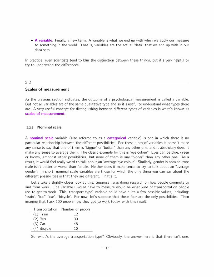
Let’s take a slightly closer look at this. Suppose I was doing research on how people commute toand from work. One variable I would have to measure would be what kind of transportation peopleuse to get to work. This “transport type” variable could have quite a few possible values, including:“train”, “bus”, “car”, “bicycle”. For now, let’s suppose that these four are the only possibilities. Thenimagine that I ask 100 people how they got to work today, with this result:

Transportation Number of people(1) Train 12(2) Bus 30(3) Car 48(4) Bicycle 10

So, what’s the average transportation type? Obviously, the answer here is that there isn’t one.

- 17 -

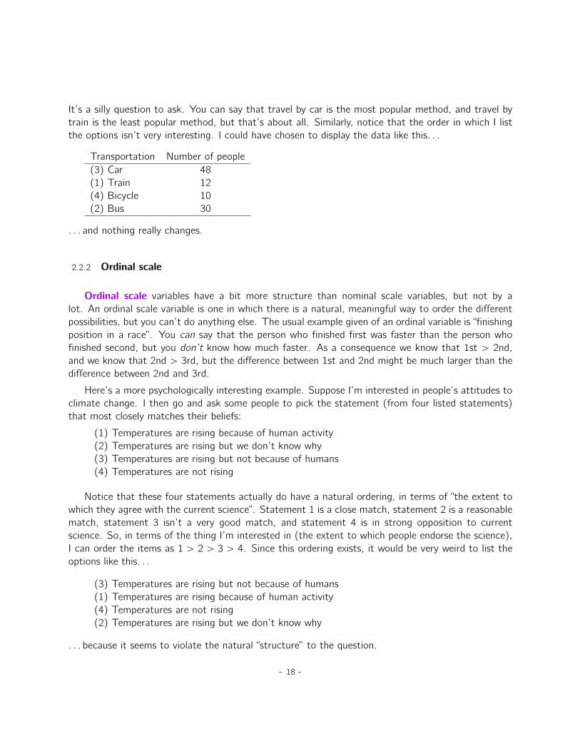
It’s a silly question to ask. You can say that travel by car is the most popular method, and travel bytrain is the least popular method, but that’s about all. Similarly, notice that the order in which I listthe options isn’t very interesting. I could have chosen to display the data like this. . .

Transportation Number of people(3) Car 48(1) Train 12(4) Bicycle 10(2) Bus 30

. . . and nothing really changes.

2.2.2 Ordinal scale

Ordinal scale variables have a bit more structure than nominal scale variables, but not by alot. An ordinal scale variable is one in which there is a natural, meaningful way to order the differentpossibilities, but you can’t do anything else. The usual example given of an ordinal variable is “finishingposition in a race”. You can say that the person who finished first was faster than the person whofinished second, but you don’t know how much faster. As a consequence we know that 1st ą 2nd,and we know that 2nd ą 3rd, but the difference between 1st and 2nd might be much larger than thedifference between 2nd and 3rd.

Here’s a more psychologically interesting example. Suppose I’m interested in people’s attitudes toclimate change. I then go and ask some people to pick the statement (from four listed statements)that most closely matches their beliefs:

(1) Temperatures are rising because of human activity(2) Temperatures are rising but we don’t know why(3) Temperatures are rising but not because of humans(4) Temperatures are not rising

Notice that these four statements actually do have a natural ordering, in terms of “the extent towhich they agree with the current science”. Statement 1 is a close match, statement 2 is a reasonablematch, statement 3 isn’t a very good match, and statement 4 is in strong opposition to currentscience. So, in terms of the thing I’m interested in (the extent to which people endorse the science),I can order the items as 1 ą 2 ą 3 ą 4. Since this ordering exists, it would be very weird to list theoptions like this. . .

(3) Temperatures are rising but not because of humans(1) Temperatures are rising because of human activity(4) Temperatures are not rising(2) Temperatures are rising but we don’t know why

. . . because it seems to violate the natural “structure” to the question.

- 18 -

So, let’s suppose I asked 100 people these questions, and got the following answers:

Response Number(1) Temperatures are rising because of human activity 51(2) Temperatures are rising but we don’t know why 20(3) Temperatures are rising but not because of humans 10(4) Temperatures are not rising 19

When analysing these data it seems quite reasonable to try to group (1), (2) and (3) together, andsay that 81 out of 100 people were willing to at least partially endorse the science. And it’s also quitereasonable to group (2), (3) and (4) together and say that 49 out of 100 people registered at leastsome disagreement with the dominant scientific view. However, it would be entirely bizarre to try togroup (1), (2) and (4) together and say that 90 out of 100 people said. . . what? There’s nothingsensible that allows you to group those responses together at all.

That said, notice that while we can use the natural ordering of these items to construct sensiblegroupings, what we can’t do is average them. For instance, in my simple example here, the “average”response to the question is 1.97. If you can tell me what that means I’d love to know, because itseems like gibberish to me!

2.2.3 Interval scale

In contrast to nominal and ordinal scale variables, interval scale and ratio scale variables arevariables for which the numerical value is genuinely meaningful. In the case of interval scale variablesthe differences between the numbers are interpretable, but the variable doesn’t have a “natural” zerovalue. A good example of an interval scale variable is measuring temperature in degrees celsius. Forinstance, if it was 15˝ yesterday and 18˝ today, then the 3˝ difference between the two is genuinelymeaningful. Moreover, that 3˝ difference is exactly the same as the 3˝ difference between 7˝ and 10˝.In short, addition and subtraction are meaningful for interval scale variables.3

However, notice that the 0˝ does not mean “no temperature at all”. It actually means “thetemperature at which water freezes”, which is pretty arbitrary. As a consequence it becomes pointlessto try to multiply and divide temperatures. It is wrong to say that 20˝ is twice as hot as 10˝, just asit is weird and meaningless to try to claim that 20˝ is negative two times as hot as ´10˝.

Again, lets look at a more psychological example. Suppose I’m interested in looking at how theattitudes of first-year university students have changed over time. Obviously, I’m going to want torecord the year in which each student started. This is an interval scale variable. A student who startedin 2003 did arrive 5 years before a student who started in 2008. However, it would be completely daft

3Actually, I’ve been informed by readers with greater physics knowledge than I that temperature isn’t strictly aninterval scale, in the sense that the amount of energy required to heat something up by 3˝ depends on it’s currenttemperature. So in the sense that physicists care about, temperature isn’t actually an interval scale. But it still makesa cute example so I’m going to ignore this little inconvenient truth.

- 19 -

for me to divide 2008 by 2003 and say that the second student started “1.0024 times later” than thefirst one. That doesn’t make any sense at all.

2.2.4 Ratio scale

The fourth and final type of variable to consider is a ratio scale variable, in which zero really meanszero, and it’s okay to multiply and divide. A good psychological example of a ratio scale variable isresponse time (RT). In a lot of tasks it’s very common to record the amount of time somebodytakes to solve a problem or answer a question, because it’s an indicator of how difficult the task is.Suppose that Alan takes 2.3 seconds to respond to a question, whereas Ben takes 3.1 seconds. Aswith an interval scale variable, addition and subtraction are both meaningful here. Ben really did take3.1 ´ 2.3 “ 0.8 seconds longer than Alan did. However, notice that multiplication and division alsomake sense here too: Ben took 3.1{2.3 “ 1.35 times as long as Alan did to answer the question. Andthe reason why you can do this is that for a ratio scale variable such as RT “zero seconds” really doesmean “no time at all”.

2.2.5 Continuous versus discrete variables

There’s a second kind of distinction that you need to be aware of, regarding what types of variablesyou can run into. This is the distinction between continuous variables and discrete variables. Thedifference between these is as follows:

• A continuous variable is one in which, for any two values that you can think of, it’s alwayslogically possible to have another value in between.

• A discrete variable is, in effect, a variable that isn’t continuous. For a discrete variable it’ssometimes the case that there’s nothing in the middle.

These definitions probably seem a bit abstract, but they’re pretty simple once you see someexamples. For instance, response time is continuous. If Alan takes 3.1 seconds and Ben takes 2.3seconds to respond to a question, then Cameron’s response time will lie in between if he took 3.0seconds. And of course it would also be possible for David to take 3.031 seconds to respond, meaningthat his RT would lie in between Cameron’s and Alan’s. And while in practice it might be impossibleto measure RT that precisely, it’s certainly possible in principle. Because we can always find a newvalue for RT in between any two other ones we regard RT as a continuous measure.

Discrete variables occur when this rule is violated. For example, nominal scale variables are alwaysdiscrete. There isn’t a type of transportation that falls “in between” trains and bicycles, not in thestrict mathematical way that 2.3 falls in between 2 and 3. So transportation type is discrete. Similarly,ordinal scale variables are always discrete. Although “2nd place” does fall between “1st place” and “3rdplace”, there’s nothing that can logically fall in between “1st place” and “2nd place”. Interval scaleand ratio scale variables can go either way. As we saw above, response time (a ratio scale variable) iscontinuous. Temperature in degrees celsius (an interval scale variable) is also continuous. However,the year you went to school (an interval scale variable) is discrete. There’s no year in between 2002

- 20 -

Table 2.1: The relationship between the scales of measurement and the discrete/continuity distinction.Cells with a tick mark correspond to things that are possible.

continuous discretenominal Xordinal Xinterval X Xratio X X

. . . . . . . . . . . . . . . . . . . . . . . . . . . . . . . . . . . . . . . . . . . . . . . . . . . . . . . . . . . . . . . . . . . . . . . . . . . . . . . . . . . . . . . . . . . .

and 2003. The number of questions you get right on a true-or-false test (a ratio scale variable) is alsodiscrete. Since a true-or-false question doesn’t allow you to be “partially correct”, there’s nothing inbetween 5/10 and 6/10. Table 2.1 summarises the relationship between the scales of measurementand the discrete/continuity distinction. Cells with a tick mark correspond to things that are possible.I’m trying to hammer this point home, because (a) some textbooks get this wrong, and (b) people veryoften say things like “discrete variable” when they mean “nominal scale variable”. It’s very unfortunate.

2.2.6 Some complexities

Okay, I know you’re going to be shocked to hear this, but the real world is much messier than thislittle classification scheme suggests. Very few variables in real life actually fall into these nice neatcategories, so you need to be kind of careful not to treat the scales of measurement as if they werehard and fast rules. It doesn’t work like that. They’re guidelines, intended to help you think aboutthe situations in which you should treat different variables differently. Nothing more.

So let’s take a classic example, maybe the classic example, of a psychological measurement tool:the Likert scale. The humble Likert scale is the bread and butter tool of all survey design. Youyourself have filled out hundreds, maybe thousands, of them and odds are you’ve even used oneyourself. Suppose we have a survey question that looks like this:

Which of the following best describes your opinion of the statement that “all pirates arefreaking awesome”?

and then the options presented to the participant are these:

(1) Strongly disagree(2) Disagree(3) Neither agree nor disagree(4) Agree(5) Strongly agree

This set of items is an example of a 5-point Likert scale, in which people are asked to choose among

- 21 -

one of several (in this case 5) clearly ordered possibilities, generally with a verbal descriptor given ineach case. However, it’s not necessary that all items are explicitly described. This is a perfectly goodexample of a 5-point Likert scale too:

(1) Strongly disagree(2)(3)(4)(5) Strongly agree

Likert scales are very handy, if somewhat limited, tools. The question is what kind of variableare they? They’re obviously discrete, since you can’t give a response of 2.5. They’re obviously notnominal scale, since the items are ordered; and they’re not ratio scale either, since there’s no naturalzero.

But are they ordinal scale or interval scale? One argument says that we can’t really prove that thedifference between “strongly agree” and “agree” is of the same size as the difference between “agree”and “neither agree nor disagree”. In fact, in everyday life it’s pretty obvious that they’re not the sameat all. So this suggests that we ought to treat Likert scales as ordinal variables. On the other hand,in practice most participants do seem to take the whole “on a scale from 1 to 5” part fairly seriously,and they tend to act as if the differences between the five response options were fairly similar to oneanother. As a consequence, a lot of researchers treat Likert scale data as interval scale.4 It’s notinterval scale, but in practice it’s close enough that we usually think of it as being quasi-interval scale.

2.3

Assessing the reliability of a measurement

At this point we’ve thought a little bit about how to operationalise a theoretical construct and therebycreate a psychological measure. And we’ve seen that by applying psychological measures we end upwith variables, which can come in many different types. At this point, we should start discussingthe obvious question: is the measurement any good? We’ll do this in terms of two related ideas:reliability and validity. Put simply, the reliability of a measure tells you how precisely you are measuringsomething, whereas the validity of a measure tells you how accurate the measure is. In this sectionI’ll talk about reliability; we’ll talk about validity in section 2.6.

Reliability is actually a very simple concept. It refers to the repeatability or consistency of yourmeasurement. The measurement of my weight by means of a “bathroom scale” is very reliable. IfI step on and off the scales over and over again, it’ll keep giving me the same answer. Measuringmy intelligence by means of “asking my mum” is very unreliable. Some days she tells me I’m a bitthick, and other days she tells me I’m a complete idiot. Notice that this concept of reliability is

4Ah, psychology . . . never an easy answer to anything!

- 22 -

different to the question of whether the measurements are correct (the correctness of a measurementrelates to it’s validity). If I’m holding a sack of potatos when I step on and off the bathroom scalesthe measurement will still be reliable: it will always give me the same answer. However, this highlyreliable answer doesn’t match up to my true weight at all, therefore it’s wrong. In technical terms,this is a reliable but invalid measurement. Similarly, whilst my mum’s estimate of my intelligence isa bit unreliable, she might be right. Maybe I’m just not too bright, and so while her estimate of myintelligence fluctuates pretty wildly from day to day, it’s basically right. That would be an unreliablebut valid measure. Of course, if my mum’s estimates are too unreliable it’s going to be very hardto figure out which one of her many claims about my intelligence is actually the right one. To someextent, then, a very unreliable measure tends to end up being invalid for practical purposes; so muchso that many people would say that reliability is necessary (but not sufficient) to ensure validity.

Okay, now that we’re clear on the distinction between reliability and validity, let’s have a thinkabout the different ways in which we might measure reliability:

• Test-retest reliability. This relates to consistency over time. If we repeat the measurement ata later date do we get a the same answer?

• Inter-rater reliability. This relates to consistency across people. If someone else repeats themeasurement (e.g., someone else rates my intelligence) will they produce the same answer?

• Parallel forms reliability. This relates to consistency across theoretically-equivalent measure-ments. If I use a different set of bathroom scales to measure my weight does it give the sameanswer?

• Internal consistency reliability. If a measurement is constructed from lots of different partsthat perform similar functions (e.g., a personality questionnaire result is added up across severalquestions) do the individual parts tend to give similar answers.

Not all measurements need to possess all forms of reliability. For instance, educational assessmentcan be thought of as a form of measurement. One of the subjects that I teach, Computational Cog-nitive Science, has an assessment structure that has a research component and an exam component(plus other things). The exam component is intended to measure something different from the re-search component, so the assessment as a whole has low internal consistency. However, within theexam there are several questions that are intended to (approximately) measure the same things, andthose tend to produce similar outcomes. So the exam on its own has a fairly high internal consistency.Which is as it should be. You should only demand reliability in those situations where you want to bemeasuring the same thing!

- 23 -

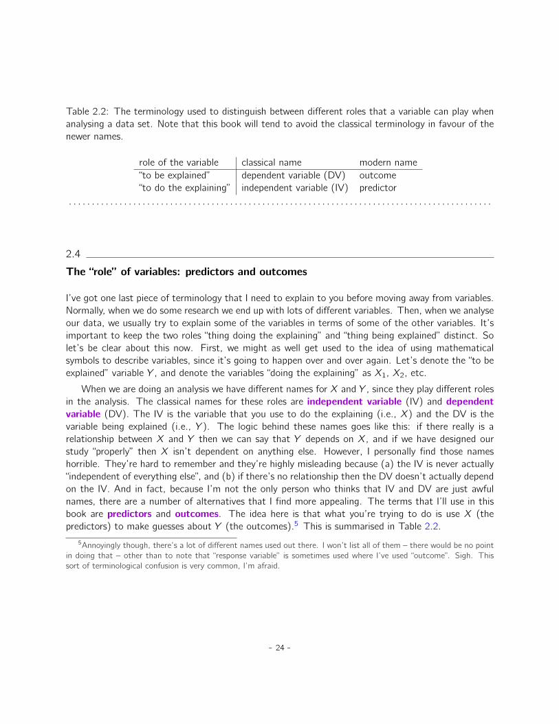
Table 2.2: The terminology used to distinguish between different roles that a variable can play whenanalysing a data set. Note that this book will tend to avoid the classical terminology in favour of thenewer names.

role of the variable classical name modern name“to be explained” dependent variable (DV) outcome“to do the explaining” independent variable (IV) predictor

. . . . . . . . . . . . . . . . . . . . . . . . . . . . . . . . . . . . . . . . . . . . . . . . . . . . . . . . . . . . . . . . . . . . . . . . . . . . . . . . . . . . . . . . . . . .

2.4

The “role” of variables: predictors and outcomes

I’ve got one last piece of terminology that I need to explain to you before moving away from variables.Normally, when we do some research we end up with lots of different variables. Then, when we analyseour data, we usually try to explain some of the variables in terms of some of the other variables. It’simportant to keep the two roles “thing doing the explaining” and “thing being explained” distinct. Solet’s be clear about this now. First, we might as well get used to the idea of using mathematicalsymbols to describe variables, since it’s going to happen over and over again. Let’s denote the “to beexplained” variable Y , and denote the variables “doing the explaining” as X1, X2, etc.

When we are doing an analysis we have different names for X and Y , since they play different rolesin the analysis. The classical names for these roles are independent variable (IV) and dependentvariable (DV). The IV is the variable that you use to do the explaining (i.e., X) and the DV is thevariable being explained (i.e., Y ). The logic behind these names goes like this: if there really is arelationship between X and Y then we can say that Y depends on X, and if we have designed ourstudy “properly” then X isn’t dependent on anything else. However, I personally find those nameshorrible. They’re hard to remember and they’re highly misleading because (a) the IV is never actually“independent of everything else”, and (b) if there’s no relationship then the DV doesn’t actually dependon the IV. And in fact, because I’m not the only person who thinks that IV and DV are just awfulnames, there are a number of alternatives that I find more appealing. The terms that I’ll use in thisbook are predictors and outcomes. The idea here is that what you’re trying to do is use X (thepredictors) to make guesses about Y (the outcomes).5 This is summarised in Table 2.2.

5Annoyingly though, there’s a lot of different names used out there. I won’t list all of them – there would be no pointin doing that – other than to note that “response variable” is sometimes used where I’ve used “outcome”. Sigh. Thissort of terminological confusion is very common, I’m afraid.

- 24 -

2.5

Experimental and non-experimental research

One of the big distinctions that you should be aware of is the distinction between “experimentalresearch” and “non-experimental research”. When we make this distinction, what we’re really talkingabout is the degree of control that the researcher exercises over the people and events in the study.

2.5.1 Experimental research

The key feature of experimental research is that the researcher controls all aspects of the study,especially what participants experience during the study. In particular, the researcher manipulatesor varies the predictor variables (IVs) but allows the outcome variable (DV) to vary naturally. Theidea here is to deliberately vary the predictors (IVs) to see if they have any causal effects on theoutcomes. Moreover, in order to ensure that there’s no possibility that something other than thepredictor variables is causing the outcomes, everything else is kept constant or is in some other way“balanced”, to ensure that they have no effect on the results. In practice, it’s almost impossible tothink of everything else that might have an influence on the outcome of an experiment, much lesskeep it constant. The standard solution to this is randomisation. That is, we randomly assign peopleto different groups, and then give each group a different treatment (i.e., assign them different valuesof the predictor variables). We’ll talk more about randomisation later, but for now it’s enough tosay that what randomisation does is minimise (but not eliminate) the possibility that there are anysystematic difference between groups.

Let’s consider a very simple, completely unrealistic and grossly unethical example. Suppose youwanted to find out if smoking causes lung cancer. One way to do this would be to find people whosmoke and people who don’t smoke and look to see if smokers have a higher rate of lung cancer. Thisis not a proper experiment, since the researcher doesn’t have a lot of control over who is and isn’t asmoker. And this really matters. For instance, it might be that people who choose to smoke cigarettesalso tend to have poor diets, or maybe they tend to work in asbestos mines, or whatever. The pointhere is that the groups (smokers and non-smokers) actually differ on lots of things, not just smoking.So it might be that the higher incidence of lung cancer among smokers is caused by something else,and not by smoking per se. In technical terms these other things (e.g. diet) are called “confounders”,and we’ll talk about those in just a moment.

In the meantime, let’s consider what a proper experiment might look like. Recall that our concernwas that smokers and non-smokers might differ in lots of ways. The solution, as long as you haveno ethics, is to control who smokes and who doesn’t. Specifically, if we randomly divide young non-smokers into two groups and force half of them to become smokers, then it’s very unlikely that thegroups will differ in any respect other than the fact that half of them smoke. That way, if our smokinggroup gets cancer at a higher rate than the non-smoking group, we can feel pretty confident that (a)

- 25 -

smoking does cause cancer and (b) we’re murderers.

2.5.2 Non-experimental research

Non-experimental research is a broad term that covers “any study in which the researcher doesn’thave as much control as they do in an experiment”. Obviously, control is something that scientistslike to have, but as the previous example illustrates there are lots of situations in which you can’t orshouldn’t try to obtain that control. Since it’s grossly unethical (and almost certainly criminal) toforce people to smoke in order to find out if they get cancer, this is a good example of a situationin which you really shouldn’t try to obtain experimental control. But there are other reasons too.Even leaving aside the ethical issues, our “smoking experiment” does have a few other issues. Forinstance, when I suggested that we “force” half of the people to become smokers, I was talking aboutstarting with a sample of non-smokers, and then forcing them to become smokers. While this soundslike the kind of solid, evil experimental design that a mad scientist would love, it might not be avery sound way of investigating the effect in the real world. For instance, suppose that smoking onlycauses lung cancer when people have poor diets, and suppose also that people who normally smokedo tend to have poor diets. However, since the “smokers” in our experiment aren’t “natural” smokers(i.e., we forced non-smokers to become smokers, but they didn’t take on all of the other normal, reallife characteristics that smokers might tend to possess) they probably have better diets. As such, inthis silly example they wouldn’t get lung cancer and our experiment will fail, because it violates thestructure of the “natural” world (the technical name for this is an “artefactual” result).

One distinction worth making between two types of non-experimental research is the differencebetween quasi-experimental research and case studies. The example I discussed earlier, in whichwe wanted to examine incidence of lung cancer among smokers and non-smokers without trying tocontrol who smokes and who doesn’t, is a quasi-experimental design. That is, it’s the same as anexperiment but we don’t control the predictors (IVs). We can still use statistics to analyse the results,but we have to be a lot more careful and circumspect.

The alternative approach, case studies, aims to provide a very detailed description of one or a fewinstances. In general, you can’t use statistics to analyse the results of case studies and it’s usuallyvery hard to draw any general conclusions about “people in general” from a few isolated examples.However, case studies are very useful in some situations. Firstly, there are situations where you don’thave any alternative. Neuropsychology has this issue a lot. Sometimes, you just can’t find a lotof people with brain damage in a specific brain area, so the only thing you can do is describe thosecases that you do have in as much detail and with as much care as you can. However, there’s alsosome genuine advantages to case studies. Because you don’t have as many people to study you havethe ability to invest lots of time and effort trying to understand the specific factors at play in eachcase. This is a very valuable thing to do. As a consequence, case studies can complement the morestatistically-oriented approaches that you see in experimental and quasi-experimental designs. We

- 26 -

won’t talk much about case studies in this book, but they are nevertheless very valuable tools!

2.6

Assessing the validity of a study

More than any other thing, a scientist wants their research to be “valid”. The conceptual idea behindvalidity is very simple. Can you trust the results of your study? If not, the study is invalid. However,whilst it’s easy to state, in practice it’s much harder to check validity than it is to check reliability.And in all honesty, there’s no precise, clearly agreed upon notion of what validity actually is. In fact,there are lots of different kinds of validity, each of which raises it’s own issues. And not all forms ofvalidity are relevant to all studies. I’m going to talk about five different types of validity:

• Internal validity

• External validity

• Construct validity

• Face validity

• Ecological validity

First, a quick guide as to what matters here. (1) Internal and external validity are the mostimportant, since they tie directly to the fundamental question of whether your study really works.(2) Construct validity asks whether you’re measuring what you think you are. (3) Face validity isn’tterribly important except insofar as you care about “appearances”. (4) Ecological validity is a specialcase of face validity that corresponds to a kind of appearance that you might care about a lot.

2.6.1 Internal validity

Internal validity refers to the extent to which you are able draw the correct conclusions aboutthe causal relationships between variables. It’s called “internal” because it refers to the relationshipsbetween things “inside” the study. Let’s illustrate the concept with a simple example. Suppose you’reinterested in finding out whether a university education makes you write better. To do so, you get agroup of first year students, ask them to write a 1000 word essay, and count the number of spellingand grammatical errors they make. Then you find some third-year students, who obviously have hadmore of a university education than the first-years, and repeat the exercise. And let’s suppose it turnsout that the third-year students produce fewer errors. And so you conclude that a university educationimproves writing skills. Right? Except that the big problem with this experiment is that the third-yearstudents are older and they’ve had more experience with writing things. So it’s hard to know for surewhat the causal relationship is. Do older people write better? Or people who have had more writingexperience? Or people who have had more education? Which of the above is the true cause of thesuperior performance of the third-years? Age? Experience? Education? You can’t tell. This is an

- 27 -

example of a failure of internal validity, because your study doesn’t properly tease apart the causalrelationships between the different variables.

2.6.2 External validity

External validity relates to the generalisability or applicability of your findings. That is, to whatextent do you expect to see the same pattern of results in “real life” as you saw in your study. Toput it a bit more precisely, any study that you do in psychology will involve a fairly specific set ofquestions or tasks, will occur in a specific environment, and will involve participants that are drawnfrom a particular subgroup (disappointingly often it is college students!). So, if it turns out that theresults don’t actually generalise or apply to people and situations beyond the ones that you studied,then what you’ve got is a lack of external validity.

The classic example of this issue is the fact that a very large proportion of studies in psychology willuse undergraduate psychology students as the participants. Obviously, however, the researchers don’tcare only about psychology students. They care about people in general. Given that, a study thatuses only psychology students as participants always carries a risk of lacking external validity. Thatis, if there’s something “special” about psychology students that makes them different to the generalpopulation in some relevant respect, then we may start worrying about a lack of external validity.

That said, it is absolutely critical to realise that a study that uses only psychology students doesnot necessarily have a problem with external validity. I’ll talk about this again later, but it’s such acommon mistake that I’m going to mention it here. The external validity of a study is threatened by thechoice of population if (a) the population from which you sample your participants is very narrow (e.g.,psychology students), and (b) the narrow population that you sampled from is systematically differentfrom the general population in some respect that is relevant to the psychological phenomenon thatyou intend to study. The italicised part is the bit that lots of people forget. It is true that psychologyundergraduates differ from the general population in lots of ways, and so a study that uses onlypsychology students may have problems with external validity. However, if those differences aren’tvery relevant to the phenomenon that you’re studying, then there’s nothing to worry about. To makethis a bit more concrete here are two extreme examples:

• You want to measure “attitudes of the general public towards psychotherapy”, but all of yourparticipants are psychology students. This study would almost certainly have a problem withexternal validity.

• You want to measure the effectiveness of a visual illusion, and your participants are all psychologystudents. This study is unlikely to have a problem with external validity

Having just spent the last couple of paragraphs focusing on the choice of participants, since that’sa big issue that everyone tends to worry most about, it’s worth remembering that external validity isa broader concept. The following are also examples of things that might pose a threat to externalvalidity, depending on what kind of study you’re doing:

• People might answer a “psychology questionnaire” in a manner that doesn’t reflect what they

- 28 -

would do in real life.

• Your lab experiment on (say) “human learning” has a different structure to the learning problemspeople face in real life.

2.6.3 Construct validity

Construct validity is basically a question of whether you’re measuring what you want to bemeasuring. A measurement has good construct validity if it is actually measuring the correct theoreticalconstruct, and bad construct validity if it doesn’t. To give a very simple (if ridiculous) example, supposeI’m trying to investigate the rates with which university students cheat on their exams. And the wayI attempt to measure it is by asking the cheating students to stand up in the lecture theatre so thatI can count them. When I do this with a class of 300 students 0 people claim to be cheaters. So Itherefore conclude that the proportion of cheaters in my class is 0%. Clearly this is a bit ridiculous.But the point here is not that this is a very deep methodological example, but rather to explain whatconstruct validity is. The problem with my measure is that while I’m trying to measure “the proportionof people who cheat” what I’m actually measuring is “the proportion of people stupid enough to ownup to cheating, or bloody minded enough to pretend that they do”. Obviously, these aren’t the samething! So my study has gone wrong, because my measurement has very poor construct validity.

2.6.4 Face validity

Face validity simply refers to whether or not a measure “looks like” it’s doing what it’s supposedto, nothing more. If I design a test of intelligence, and people look at it and they say “no, that testdoesn’t measure intelligence”, then the measure lacks face validity. It’s as simple as that. Obviously,face validity isn’t very important from a pure scientific perspective. After all, what we care about iswhether or not the measure actually does what it’s supposed to do, not whether it looks like it doeswhat it’s supposed to do. As a consequence, we generally don’t care very much about face validity.That said, the concept of face validity serves three useful pragmatic purposes:

• Sometimes, an experienced scientist will have a “hunch” that a particular measure won’t work.While these sorts of hunches have no strict evidentiary value, it’s often worth paying attentionto them. Because often times people have knowledge that they can’t quite verbalise, so theremight be something to worry about even if you can’t quite say why. In other words, whensomeone you trust criticises the face validity of your study, it’s worth taking the time to thinkmore carefully about your design to see if you can think of reasons why it might go awry. Mindyou, if you don’t find any reason for concern, then you should probably not worry. After all, facevalidity really doesn’t matter very much.

• Often (very often), completely uninformed people will also have a “hunch” that your research iscrap. And they’ll criticise it on the internet or something. On close inspection you may noticethat these criticisms are actually focused entirely on how the study “looks”, but not on anything

- 29 -

deeper. The concept of face validity is useful for gently explaining to people that they need tosubstantiate their arguments further.

• Expanding on the last point, if the beliefs of untrained people are critical (e.g., this is often thecase for applied research where you actually want to convince policy makers of something orother) then you have to care about face validity. Simply because, whether you like it or not, a lotof people will use face validity as a proxy for real validity. If you want the government to changea law on scientific psychological grounds, then it won’t matter how good your studies “really”are. If they lack face validity you’ll find that politicians ignore you. Of course, it’s somewhatunfair that policy often depends more on appearance than fact, but that’s how things go.

2.6.5 Ecological validity

Ecological validity is a different notion of validity, which is similar to external validity, but lessimportant. The idea is that, in order to be ecologically valid, the entire set up of the study shouldclosely approximate the real world scenario that is being investigated. In a sense, ecological validityis a kind of face validity. It relates mostly to whether the study “looks” right, but with a bit morerigour to it. To be ecologically valid the study has to look right in a fairly specific way. The ideabehind it is the intuition that a study that is ecologically valid is more likely to be externally valid.It’s no guarantee, of course. But the nice thing about ecological validity is that it’s much easier tocheck whether a study is ecologically valid than it is to check whether a study is externally valid. Asimple example would be eyewitness identification studies. Most of these studies tend to be done ina university setting, often with a fairly simple array of faces to look at, rather than a line up. Thelength of time between seeing the “criminal” and being asked to identify the suspect in the “line up” isusually shorter. The “crime” isn’t real so there’s no chance of the witness being scared, and there areno police officers present so there’s not as much chance of feeling pressured. These things all meanthat the study definitely lacks ecological validity. They might (but might not) mean that it also lacksexternal validity.

2.7

Confounds, artefacts and other threats to validity

If we look at the issue of validity in the most general fashion the two biggest worries that we have areconfounders and artefacts. These two terms are defined in the following way:

- 30 -

• Confounder: A confounder is an additional, often unmeasured variable6 that turns out to berelated to both the predictors and the outcome. The existence of confounders threatens theinternal validity of the study because you can’t tell whether the predictor causes the outcome,or if the confounding variable causes it.

• Artefact: A result is said to be “artefactual” if it only holds in the special situation that youhappened to test in your study. The possibility that your result is an artefact describes a threatto your external validity, because it raises the possibility that you can’t generalise or apply yourresults to the actual population that you care about.

As a general rule confounders are a bigger concern for non-experimental studies, precisely becausethey’re not proper experiments. By definition, you’re leaving lots of things uncontrolled, so there’sa lot of scope for confounders being present in your study. Experimental research tends to be muchless vulnerable to confounders. The more control you have over what happens during the study, themore you can prevent confounders from affecting the results. With random allocation, for example,confounders are distributed randomly, and evenly, between different groups.

However, there are always swings and roundabouts and when we start thinking about artefactsrather than confounders the shoe is very firmly on the other foot. For the most part, artefactualresults tend to be a concern for experimental studies than for non-experimental studies. To see this, ithelps to realise that the reason that a lot of studies are non-experimental is precisely because what theresearcher is trying to do is examine human behaviour in a more naturalistic context. By working ina more real-world context you lose experimental control (making yourself vulnerable to confounders),but because you tend to be studying human psychology “in the wild” you reduce the chances of gettingan artefactual result. Or, to put it another way, when you take psychology out of the wild and bringit into the lab (which we usually have to do to gain our experimental control), you always run the riskof accidentally studying something different to what you wanted to study.

Be warned though. The above is a rough guide only. It’s absolutely possible to have confoundersin an experiment, and to get artefactual results with non-experimental studies. This can happen forall sorts of reasons, not least of which is experimenter or researcher error. In practice, it’s really hardto think everything through ahead of time and even very good researchers make mistakes.

Although there’s a sense in which almost any threat to validity can be characterised as a confounderor an artefact, they’re pretty vague concepts. So let’s have a look at some of the most commonexamples.

2.7.1 History effects

History effects refer to the possibility that specific events may occur during the study that might6The reason why I say that it’s unmeasured is that if you have measured it, then you can use some fancy statistical

tricks to deal with the confounder. Because of the existence of these statistical solutions to the problem of confounders,we often refer to a confounder that we have measured and dealt with as a covariate. Dealing with covariates is a moreadvanced topic, but I thought I’d mention it in passing since it’s kind of comforting to at least know that this stuff exists.

- 31 -

influence the outcome measure. For instance, something might happen in between a pre-test and apost-test. Or in-between testing participant 23 and participant 24. Alternatively, it might be thatyou’re looking at a paper from an older study that was perfectly valid for its time, but the world haschanged enough since then that the conclusions are no longer trustworthy. Examples of things thatwould count as history effects are:

• You’re interested in how people think about risk and uncertainty. You started your data collectionin December 2010. But finding participants and collecting data takes time, so you’re still findingnew people in February 2011. Unfortunately for you (and even more unfortunately for others),the Queensland floods occurred in January 2011 causing billions of dollars of damage and killingmany people. Not surprisingly, the people tested in February 2011 express quite different beliefsabout handling risk than the people tested in December 2010. Which (if any) of these reflectsthe “true” beliefs of participants? I think the answer is probably both. The Queensland floodsgenuinely changed the beliefs of the Australian public, though possibly only temporarily. Thekey thing here is that the “history” of the people tested in February is quite different to peopletested in December.

• You’re testing the psychological effects of a new anti-anxiety drug. So what you do is measureanxiety before administering the drug (e.g., by self-report, and taking physiological measures).Then you administer the drug, and afterwards you take the same measures. In the middlehowever, because your lab is in Los Angeles, there’s an earthquake which increases the anxietyof the participants.

2.7.2 Maturation effects

As with history effects, maturational effects are fundamentally about change over time. However,maturation effects aren’t in response to specific events. Rather, they relate to how people change ontheir own over time. We get older, we get tired, we get bored, etc. Some examples of maturationeffects are:

• When doing developmental psychology research you need to be aware that children grow upquite rapidly. So, suppose that you want to find out whether some educational trick helps withvocabulary size among 3 year olds. One thing that you need to be aware of is that the vocabularysize of children that age is growing at an incredible rate (multiple words per day) all on its own.If you design your study without taking this maturational effect into account, then you won’tbe able to tell if your educational trick works.

• When running a very long experiment in the lab (say, something that goes for 3 hours) it’s verylikely that people will begin to get bored and tired, and that this maturational effect will causeperformance to decline regardless of anything else going on in the experiment

- 32 -

2.7.3 Repeated testing effects

An important type of history effect is the effect of repeated testing. Suppose I want to take twomeasurements of some psychological construct (e.g., anxiety). One thing I might be worried about isif the first measurement has an effect on the second measurement. In other words, this is a historyeffect in which the “event” that influences the second measurement is the first measurement itself!This is not at all uncommon. Examples of this include:

• Learning and practice: e.g., “intelligence” at time 2 might appear to go up relative to time 1because participants learned the general rules of how to solve “intelligence-test-style” questionsduring the first testing session.

• Familiarity with the testing situation: e.g., if people are nervous at time 1, this might makeperformance go down. But after sitting through the first testing situation they might calmdown a lot precisely because they’ve seen what the testing looks like.

• Auxiliary changes caused by testing: e.g., if a questionnaire assessing mood is boring thenmood rating at measurement time 2 is more likely to be “bored” precisely because of the boringmeasurement made at time 1.

2.7.4 Selection bias

Selection bias is a pretty broad term. Suppose that you’re running an experiment with two groupsof participants where each group gets a different “treatment”, and you want to see if the differenttreatments lead to different outcomes. However, suppose that, despite your best efforts, you’veended up with a gender imbalance across groups (say, group A has 80% females and group B has50% females). It might sound like this could never happen but, trust me, it can. This is an exampleof a selection bias, in which the people “selected into” the two groups have different characteristics.If any of those characteristics turns out to be relevant (say, your treatment works better on femalesthan males) then you’re in a lot of trouble.

2.7.5 Differential attrition

When thinking about the effects of attrition, it is sometimes helpful to distinguish between twodifferent types. The first is homogeneous attrition, in which the attrition effect is the same for allgroups, treatments or conditions. In the example I gave above, the attrition would be homogeneous if(and only if) the easily bored participants are dropping out of all of the conditions in my experiment atabout the same rate. In general, the main effect of homogeneous attrition is likely to be that it makesyour sample unrepresentative. As such, the biggest worry that you’ll have is that the generalisabilityof the results decreases. In other words, you lose external validity.

The second type of attrition is heterogeneous attrition, in which the attrition effect is differentfor different groups. More often called differential attrition, this is a kind of selection bias that is

- 33 -

caused by the study itself. Suppose that, for the first time ever in the history of psychology, I manageto find the perfectly balanced and representative sample of people. I start running “Dani’s incrediblylong and tedious experiment” on my perfect sample but then, because my study is incredibly long andtedious, lots of people start dropping out. I can’t stop this. Participants absolutely have the rightto stop doing any experiment, any time, for whatever reason they feel like, and as researchers we aremorally (and professionally) obliged to remind people that they do have this right. So, suppose that“Dani’s incredibly long and tedious experiment” has a very high drop out rate. What do you supposethe odds are that this drop out is random? Answer: zero. Almost certainly the people who remainare more conscientious, more tolerant of boredom, etc., than those that leave. To the extent that(say) conscientiousness is relevant to the psychological phenomenon that I care about, this attritioncan decrease the validity of my results.

Here’s another example. Suppose I design my experiment with two conditions. In the “treatment”condition, the experimenter insults the participant and then gives them a questionnaire designed tomeasure obedience. In the “control” condition, the experimenter engages in a bit of pointless chitchatand then gives them the questionnaire. Leaving aside the questionable scientific merits and dubiousethics of such a study, let’s have a think about what might go wrong here. As a general rule, whensomeone insults me to my face I tend to get much less co-operative. So, there’s a pretty good chancethat a lot more people are going to drop out of the treatment condition than the control condition.And this drop out isn’t going to be random. The people most likely to drop out would probablybe the people who don’t care all that much about the importance of obediently sitting through theexperiment. Since the most bloody minded and disobedient people all left the treatment group butnot the control group, we’ve introduced a confound: the people who actually took the questionnaire inthe treatment group were already more likely to be dutiful and obedient than the people in the controlgroup. In short, in this study insulting people doesn’t make them more obedient. It makes the moredisobedient people leave the experiment! The internal validity of this experiment is completely shot.

2.7.6 Non-response bias

Non-response bias is closely related to selection bias and to differential attrition. The simplestversion of the problem goes like this. You mail out a survey to 1000 people but only 300 of themreply. The 300 people who replied are almost certainly not a random subsample. People who respondto surveys are systematically different to people who don’t. This introduces a problem when tryingto generalise from those 300 people who replied to the population at large, since you now have avery non-random sample. The issue of non-response bias is more general than this, though. Amongthe (say) 300 people that did respond to the survey, you might find that not everyone answers everyquestion. If (say) 80 people chose not to answer one of your questions, does this introduce problems?As always, the answer is maybe. If the question that wasn’t answered was on the last page of thequestionnaire, and those 80 surveys were returned with the last page missing, there’s a good chancethat the missing data isn’t a big deal; probably the pages just fell off. However, if the question that 80people didn’t answer was the most confrontational or invasive personal question in the questionnaire,then almost certainly you’ve got a problem. In essence, what you’re dealing with here is what’s calledthe problem of missing data. If the data that is missing was “lost” randomly, then it’s not a big

- 34 -

problem. If it’s missing systematically, then it can be a big problem.

2.7.7 Regression to the mean

Regression to the mean refers to any situation where you select data based on an extreme valueon some measure. Because the variable has natural variation it almost certainly means that when youtake a subsequent measurement the later measurement will be less extreme than the first one, purelyby chance.

Here’s an example. Suppose I’m interested in whether a psychology education has an adverseeffect on very smart kids. To do this, I find the 20 psychology I students with the best high schoolgrades and look at how well they’re doing at university. It turns out that they’re doing a lot betterthan average, but they’re not topping the class at university even though they did top their classes athigh school. What’s going on? The natural first thought is that this must mean that the psychologyclasses must be having an adverse effect on those students. However, while that might very well bethe explanation, it’s more likely that what you’re seeing is an example of “regression to the mean”. Tosee how it works, let’s take a moment to think about what is required to get the best mark in a class,regardless of whether that class be at high school or at university. When you’ve got a big class thereare going to be lots of very smart people enrolled. To get the best mark you have to be very smart,work very hard, and be a bit lucky. The exam has to ask just the right questions for your idiosyncraticskills, and you have to avoid making any dumb mistakes (we all do that sometimes) when answeringthem. And that’s the thing, whilst intelligence and hard work are transferable from one class to thenext, luck isn’t. The people who got lucky in high school won’t be the same as the people who getlucky at university. That’s the very definition of “luck”. The consequence of this is that when youselect people at the very extreme values of one measurement (the top 20 students), you’re selectingfor hard work, skill and luck. But because the luck doesn’t transfer to the second measurement (onlythe skill and work), these people will all be expected to drop a little bit when you measure them asecond time (at university). So their scores fall back a little bit, back towards everyone else. This isregression to the mean.

Regression to the mean is surprisingly common. For instance, if two very tall people have kidstheir children will tend to be taller than average but not as tall as the parents. The reverse happenswith very short parents. Two very short parents will tend to have short children, but neverthelessthose kids will tend to be taller than the parents. It can also be extremely subtle. For instance,there have been studies done that suggested that people learn better from negative feedback thanfrom positive feedback. However, the way that people tried to show this was to give people positivereinforcement whenever they did good, and negative reinforcement when they did bad. And whatyou see is that after the positive reinforcement people tended to do worse, but after the negativereinforcement they tended to do better. But notice that there’s a selection bias here! When peopledo very well, you’re selecting for “high” values, and so you should expect, because of regression to themean, that performance on the next trial should be worse regardless of whether reinforcement is given.Similarly, after a bad trial, people will tend to improve all on their own. The apparent superiority ofnegative feedback is an artefact caused by regression to the mean (see Kahneman and Tversky 1973,

- 35 -

for discussion).

2.7.8 Experimenter bias

Experimenter bias can come in multiple forms. The basic idea is that the experimenter, despitethe best of intentions, can accidentally end up influencing the results of the experiment by subtlycommunicating the “right answer” or the “desired behaviour” to the participants. Typically, this occursbecause the experimenter has special knowledge that the participant does not, for example the rightanswer to the questions being asked or knowledge of the expected pattern of performance for thecondition that the participant is in. The classic example of this happening is the case study of “CleverHans”, which dates back to 1907 (Pfungst 1911; Hothersall 2004). Clever Hans was a horse thatapparently was able to read and count and perform other human like feats of intelligence. AfterClever Hans became famous, psychologists started examining his behaviour more closely. It turnedout that, not surprisingly, Hans didn’t know how to do maths. Rather, Hans was responding to thehuman observers around him, because the humans did know how to count and the horse had learnedto change its behaviour when people changed theirs.

The general solution to the problem of experimenter bias is to engage in double blind studies, whereneither the experimenter nor the participant knows which condition the participant is in or knows whatthe desired behaviour is. This provides a very good solution to the problem, but it’s important torecognise that it’s not quite ideal, and hard to pull off perfectly. For instance, the obvious way that Icould try to construct a double blind study is to have one of my Ph.D. students (one who doesn’t knowanything about the experiment) run the study. That feels like it should be enough. The only person(me) who knows all the details (e.g., correct answers to the questions, assignments of participantsto conditions) has no interaction with the participants, and the person who does all the talking topeople (the Ph.D. student) doesn’t know anything. Except for the reality that the last part is veryunlikely to be true. In order for the Ph.D. student to run the study effectively they need to havebeen briefed by me, the researcher. And, as it happens, the Ph.D. student also knows me and knowsa bit about my general beliefs about people and psychology (e.g., I tend to think humans are muchsmarter than psychologists give them credit for). As a result of all this, it’s almost impossible forthe experimenter to avoid knowing a little bit about what expectations I have. And even a little bitof knowledge can have an effect. Suppose the experimenter accidentally conveys the fact that theparticipants are expected to do well in this task. Well, there’s a thing called the “Pygmalion effect”,where if you expect great things of people they’ll tend to rise to the occasion. But if you expect themto fail then they’ll do that too. In other words, the expectations become a self-fulfilling prophesy.

2.7.9 Demand effects and reactivity

When talking about experimenter bias, the worry is that the experimenter’s knowledge or desires forthe experiment are communicated to the participants, and that these can change people’s behaviour(Rosenthal 1966). However, even if you manage to stop this from happening, it’s almost impossibleto stop people from knowing that they’re part of a psychological study. And the mere fact of knowingthat someone is watching or studying you can have a pretty big effect on behaviour. This is generally

- 36 -

referred to as reactivity or demand effects. The basic idea is captured by the Hawthorne effect:people alter their performance because of the attention that the study focuses on them. The effecttakes its name from a study that took place in the “Hawthorne Works” factory outside of Chicago(see Adair 1984). This study, from the 1920s, looked at the effects of factory lighting on workerproductivity. But, importantly, change in worker behaviour occurred because the workers knew theywere being studied, rather than any effect of factory lighting.

To get a bit more specific about some of the ways in which the mere fact of being in a study canchange how people behave, it helps to think like a social psychologist and look at some of the rolesthat people might adopt during an experiment but might not adopt if the corresponding events wereoccurring in the real world:

• The good participant tries to be too helpful to the researcher. He or she seeks to figure out theexperimenter’s hypotheses and confirm them.

• The negative participant does the exact opposite of the good participant. He or she seeks tobreak or destroy the study or the hypothesis in some way.

• The faithful participant is unnaturally obedient. He or she seeks to follow instructions perfectly,regardless of what might have happened in a more realistic setting.

• The apprehensive participant gets nervous about being tested or studied, so much so that hisor her behaviour becomes highly unnatural, or overly socially desirable.

2.7.10 Placebo effects

The placebo effect is a specific type of demand effect that we worry a lot about. It refers tothe situation where the mere fact of being treated causes an improvement in outcomes. The classicexample comes from clinical trials. If you give people a completely chemically inert drug and tell themthat it’s a cure for a disease, they will tend to get better faster than people who aren’t treated at all.In other words, it is people’s belief that they are being treated that causes the improved outcomes,not the drug.

However, the current consensus in medicine is that true placebo effects are quite rare and most ofwhat was previously considered placebo effect is in fact some combination of natural healing (somepeople just get better on their own), regression to the mean and other quirks of study design. Ofinterest to psychology is that the strongest evidence for at least some placebo effect is in self-reportedoutcomes, most notably in treatment of pain (Hróbjartsson and Gøtzsche 2010).

2.7.11 Situation, measurement and sub-population effects

In some respects, these terms are a catch-all term for “all other threats to external validity”. Theyrefer to the fact that the choice of sub-population from which you draw your participants, the location,timing and manner in which you run your study (including who collects the data) and the tools that

- 37 -

you use to make your measurements might all be influencing the results. Specifically, the worry is thatthese things might be influencing the results in such a way that the results won’t generalise to a widerarray of people, places and measures.

2.7.12 Fraud, deception and self-deception

It is difficult to get a man to understand something, when his salary depends on his notunderstanding it.

– Upton Sinclair

There’s one final thing I feel I should mention. While reading what the textbooks often have tosay about assessing the validity of a study I couldn’t help but notice that they seem to make theassumption that the researcher is honest. I find this hilarious. While the vast majority of scientistsare honest, in my experience at least, some are not.7 Not only that, as I mentioned earlier, scientistsare not immune to belief bias. It’s easy for a researcher to end up deceiving themselves into believingthe wrong thing, and this can lead them to conduct subtly flawed research and then hide those flawswhen they write it up. So you need to consider not only the (probably unlikely) possibility of outrightfraud, but also the (probably quite common) possibility that the research is unintentionally “slanted”.I opened a few standard textbooks and didn’t find much of a discussion of this problem, so here’s myown attempt to list a few ways in which these issues can arise:

• Data fabrication. Sometimes, people just make up the data. This is occasionally done with“good” intentions. For instance, the researcher believes that the fabricated data do reflect thetruth, and may actually reflect “slightly cleaned up” versions of actual data. On other occasions,the fraud is deliberate and malicious. Some high-profile examples where data fabrication hasbeen alleged or shown include Cyril Burt (a psychologist who is thought to have fabricated someof his data), Andrew Wakefield (who has been accused of fabricating his data connecting theMMR vaccine to autism) and Hwang Woo-suk (who falsified a lot of his data on stem cellresearch).

• Hoaxes. Hoaxes share a lot of similarities with data fabrication, but they differ in the intendedpurpose. A hoax is often a joke, and many of them are intended to be (eventually) discovered.Often, the point of a hoax is to discredit someone or some field. There’s quite a few wellknown scientific hoaxes that have occurred over the years (e.g., Piltdown man) and some weredeliberate attempts to discredit particular fields of research (e.g., the Sokal affair).

• Data misrepresentation. While fraud gets most of the headlines, it’s much more common inmy experience to see data being misrepresented. When I say this I’m not referring to newspapersgetting it wrong (which they do, almost always). I’m referring to the fact that often the data

7Some people might argue that if you’re not honest then you’re not a real scientist. Which does have some truth toit I guess, but that’s disingenuous (look up the “No true Scotsman” fallacy). The fact is that there are lots of people whoare employed ostensibly as scientists, and whose work has all of the trappings of science, but who are outright fraudulent.Pretending that they don’t exist by saying that they’re not scientists is just muddled thinking.

- 38 -

don’t actually say what the researchers think they say. My guess is that, almost always, thisisn’t the result of deliberate dishonesty but instead is due to a lack of sophistication in the dataanalyses. For instance, think back to the example of Simpson’s paradox that I discussed in thebeginning of this book. It’s very common to see people present “aggregated” data of some kindand sometimes, when you dig deeper and find the raw data yourself you find that the aggregateddata tell a different story to the disaggregated data. Alternatively, you might find that someaspect of the data is being hidden, because it tells an inconvenient story (e.g., the researchermight choose not to refer to a particular variable). There’s a lot of variants on this, many ofwhich are very hard to detect.

• Study “misdesign” . Okay, this one is subtle. Basically, the issue here is that a researcherdesigns a study that has built-in flaws and those flaws are never reported in the paper. Thedata that are reported are completely real and are correctly analysed, but they are producedby a study that is actually quite wrongly put together. The researcher really wants to find aparticular effect and so the study is set up in such a way as to make it “easy” to (artefactually)observe that effect. One sneaky way to do this, in case you’re feeling like dabbling in a bit offraud yourself, is to design an experiment in which it’s obvious to the participants what they’re“supposed” to be doing, and then let reactivity work its magic for you. If you want you can addall the trappings of double blind experimentation but it won’t make a difference since the studymaterials themselves are subtly telling people what you want them to do. When you write up theresults the fraud won’t be obvious to the reader. What’s obvious to the participant when they’rein the experimental context isn’t always obvious to the person reading the paper. Of course,the way I’ve described this makes it sound like it’s always fraud. Probably there are cases wherethis is done deliberately, but in my experience the bigger concern has been with unintentionalmisdesign. The researcher believes and so the study just happens to end up with a built in flaw,and that flaw then magically erases itself when the study is written up for publication.

• Data mining & post hoc hypothesising. Another way in which the authors of a study canmore or less misrepresent the data is by engaging in what’s referred to as “data mining” (seeGelman and Loken 2014, for a broader discussion of this as part of the “garden of forking paths”in statistical analysis). As we’ll discuss later, if you keep trying to analyse your data in lots ofdifferent ways, you’ll eventually find something that “looks” like a real effect but isn’t. This isreferred to as “data mining”. It used to be quite rare because data analysis used to take weeks,but now that everyone has very powerful statistical software on their computers it’s becomingvery common. Data mining per se isn’t “wrong”, but the more that you do it the bigger the riskyou’re taking. The thing that is wrong, and I suspect is very common, is unacknowledged datamining. That is, the researcher runs every possible analysis known to humanity, finds the onethat works, and then pretends that this was the only analysis that they ever conducted. Worseyet, they often “invent” a hypothesis after looking at the data to cover up the data mining. Tobe clear. It’s not wrong to change your beliefs after looking at the data, and to reanalyse yourdata using your new “post hoc” hypotheses. What is wrong (and I suspect common) is failingto acknowledge that you’ve done. If you acknowledge that you did it then other researchers areable to take your behaviour into account. If you don’t, then they can’t. And that makes your

- 39 -

behaviour deceptive. Bad!

• Publication bias & self-censoring. Finally, a pervasive bias is “non-reporting” of negative results.This is almost impossible to prevent. Journals don’t publish every article that is submitted tothem. They prefer to publish articles that find “something”. So, if 20 people run an experimentlooking at whether reading Finnegans Wake causes insanity in humans, and 19 of them find thatit doesn’t, which one do you think is going to get published? Obviously, it’s the one study thatdid find that Finnegans Wake causes insanity.8 This is an example of a publication bias. Sinceno-one ever published the 19 studies that didn’t find an effect, a naive reader would never knowthat they existed. Worse yet, most researchers “internalise” this bias and end up self-censoringtheir research. Knowing that negative results aren’t going to be accepted for publication, theynever even try to report them. As a friend of mine says “for every experiment that you getpublished, you also have 10 failures”. And she’s right. The catch is, while some (maybe most)of those studies are failures for boring reasons (e.g. you stuffed something up) others might begenuine “null” results that you ought to acknowledge when you write up the “good” experiment.And telling which is which is often hard to do. A good place to start is a paper by Ioannidis(2005) with the depressing title “Why most published research findings are false”. I’d also suggesttaking a look at work by Kühberger, Fritz, and Scherndl (2014) presenting statistical evidencethat this actually happens in psychology.

There’s probably a lot more issues like this to think about, but that’ll do to start with. What Ireally want to point out is the blindingly obvious truth that real world science is conducted by actualhumans, and only the most gullible of people automatically assumes that everyone else is honest andimpartial. Actual scientists aren’t usually that naive, but for some reason the world likes to pretendthat we are, and the textbooks we usually write seem to reinforce that stereotype.

2.8

Summary

This chapter isn’t really meant to provide a comprehensive discussion of psychological research meth-ods. It would require another volume just as long as this one to do justice to the topic. However, inreal life statistics and study design are so tightly intertwined that it’s very handy to discuss some ofthe key topics. In this chapter, I’ve briefly discussed the following topics:

• Introduction to psychological measurement (Section 2.1). What does it mean to operationalisea theoretical construct? What does it mean to have variables and take measurements?

• Scales of measurement and types of variables (Section 2.2). Remember that there are twodifferent distinctions here. There’s the difference between discrete and continuous data, andthere’s the difference between the four different scale types (nominal, ordinal, interval and ratio).

8Clearly, the real effect is that only insane people would even try to read Finnegans Wake.

- 40 -

• Reliability of a measurement (Section 2.3). If I measure the “same” thing twice, should I expectto see the same result? Only if my measure is reliable. But what does it mean to talk aboutdoing the “same” thing? Well, that’s why we have different types of reliability. Make sure youremember what they are.

• Terminology: predictors and outcomes (Section 2.4). What roles do variables play in an analysis?Can you remember the difference between predictors and outcomes? Dependent and independentvariables? Etc.

• Experimental and non-experimental research designs (Section 2.5). What makes an experimentan experiment? Is it a nice white lab coat, or does it have something to do with researchercontrol over variables?

• Validity and its threats (Section 2.6). Does your study measure what you want it to? Howmight things go wrong? And is it my imagination, or was that a very long list of possible waysin which things can go wrong?

All this should make clear to you that study design is a critical part of research methodology. Ibuilt this chapter from the classic little book by Campbell et al. (1963), but there are of course a largenumber of textbooks out there on research design. Spend a few minutes with your favourite searchengine and you’ll find dozens.

- 41 -

- 42 -

Part II.

Describing and displaying data with JASP

- 43 -

3. Getting started with JASP

Robots are nice to work with.–Roger Zelazny1

In this chapter we’ll discuss how to get started in JASP. We’ll briefly talk about how to downloadand install JASP, but most of the chapter will be focused on getting you started with finding yourway around the JASP user interface. Our goal in this chapter is not to learn any statistical concepts:instead, we’re just trying to learn the basics of how JASP works and get comfortable interacting withthe system. To do this we’ll spend some time looking at datasets and variables. In doing so, you’llget a bit of a feel for what it’s like to work in JASP.

However, before going into any of the specifics, it’s worth talking a little about why you might wantto use JASP at all. Given that you’re reading this you’ve probably got your own reasons. However, ifthose reasons are “because that’s what my stats class uses”, it might be worth explaining a little whyyour professor has chosen to use JASP for the class. Of course, who really knows why other peoplechoose JASP, so really, I will be talking about why I use it.

• It’s sort of obvious but worth saying anyway: doing statistics on a computer is faster, easierand more powerful than doing statistics by hand. Computers excel at mindless repetitive tasks,and a lot of statistical calculations are both mindless and repetitive. For most people the onlyreason to ever do statistical calculations with pencil and paper is for learning purposes (evenprofessionals do this when learning new concepts). In my class I do occasionally suggest doingsome calculations that way, but the only real value to it is pedagogical. It does help you to get a“feel” for statistics to do some calculations yourself, so it’s worth doing it once. But only once!

• Doing statistics in a conventional spreadsheet (e.g., Microsoft Excel) is generally a bad idea inthe long run. Although many people likely feel more familiar with them, spreadsheets are verylimited in terms of what analyses they allow you do. If you get into the habit of trying to doyour real life data analysis using spreadsheets then you’ve dug yourself into a very deep hole.

• Avoiding proprietary software is a very good idea. There are a lot of commercial packages outthere that you can buy, some of which I like and some of which I don’t. They’re usually very

1Source: Dismal Light (1968).

- 45 -

glossy in their appearance and generally very powerful (much more powerful than spreadsheets).However, they’re also very expensive. Usually, the company sells “student versions” (crippledversions of the real thing) very cheaply, and then they they sell full powered “educational versions”at a price that makes me wince. They will also sell commercial licences with a staggeringly highprice tag. The business model here is to suck you in during your student days and then leaveyou dependent on their tools when you go out into the real world. It’s hard to blame them fortrying, but personally I’m not in favor of shelling out thousands of dollars if I can avoid it. Andyou can avoid it. If you make use of packages like JASP that are open source and free you neverget trapped having to pay exorbitant licensing fees.

Those are the main reasons I use JASP. It’s not without its flaws, though. It’s relatively new2 so thereis not a huge set of textbooks and other resources to support it, and it has a few annoying quirks thatwe’re all pretty much stuck with, but on the whole I think the strengths outweigh the weakness; moreso than any other option I’ve encountered so far.

3.1

Installing JASP

Okay, enough with the sales pitch. Let’s get started. Just as with any piece of software, JASP needsto be installed on a computer. Fortunately, JASP is freely distributed online and you can download itfrom the JASP homepage, which is:

https://jasp-stats.org/

At the top of the page, you’ll click on the heading “Download”. Then, you’ll see separate links forWindows users, Mac users, and Linux users. If you follow the relevant link you’ll see that the onlineinstructions are pretty self-explanatory. As of this writing, the current version of JASP is 0.9.2.0, butthey usually issue updates every few months, so you’ll probably have a newer version.3

3.1.1 Starting up JASP

One way or another, regardless of what operating system you’re using, it’s time to open JASPand get started. When first starting JASP you will be presented with a user interface which lookssomething like Figure 3.1.

If you have experience with other statistical software packages, you might be a bit dismayed to seethat there is no place to begin typing your data. This is a deliberate decision on the part of the JASP

2As of writing this in May 2019.3Although JASP is updated frequently it doesn’t usually make much of a difference for the sort of work we’ll do in

this book. In fact, during the writing of the book I upgraded several times and it didn’t make much difference at all towhat is in this book.

- 46 -

https://jasp-stats.org/

Figure 3.1: JASP looks like this when you start it.

developers; their philosophy is that users should be allowed to use the editor they are most comfortablewith 4. Thus, the preferred method for getting data into JASP is to load a CSV file (.csv), whichis a text-based data format that can be created by (and opened in) any spreadsheet program. Moredetails about this will be given shortly.

3.2

Analyses

Analyses can be selected from several buttons along the top. Selecting an analysis will present an‘options panel’ for that particular analysis, allowing you to assign different variables to different partsof the analysis, and select different options. At the same time, the results for the analysis will appearin the right ‘Results panel’ and will update in real-time as you make changes to the options.

When you have the analysis set up correctly you can dismiss the analysis options by clicking the4See https://jasp-stats.org/2018/05/15/data-editing-in-jasp/ for a discussion of this very issue.

- 47 -

’OK’ button in the top right of the optional panel. If you wish to return to these options, you canclick on the results that were produced. In this way, you can return to any analysis that you (or say,a colleague) created earlier.

If you decide you no longer need a particular analysis, you can remove it with the results contextmenu. Clicking on the header of a specific results header (or clicking on the İ symbol) will bring up amenu and by selecting ‘Remove Analysis’, the analysis can be removed. But more on this later. First,let’s get some data into JASP.

3.3

Loading data in JASP

There are several different types of files that are likely to be relevant to us when doing data analysis.There are two in particular that are especially important from the perspective of this book:

• .jasp files are those with a .jasp file extension. This is the standard kind of file that JASP usesto store data, and variables and analyses.

• Comma separated value (CSV) files are those with a .csv file extension. These are just regularold text files and they can be opened with many different software programs. It’s quite typicalfor people to store data in csv files, precisely because they’re so simple.

3.3.1 Importing data from CSV files

One quite commonly used data format is the humble “comma separated value” file, also called aCSV file, and usually bearing the file extension .csv. CSV files are just plain old-fashioned text filesand what they store is basically just a table of data. This is illustrated in Figure 3.2, which shows afile called booksales.csv that I’ve created. As you can see, each row represents the book sales datafor one month. The first row doesn’t contain actual data though, it has the names of the variables.

Once you have a CSV file (either that you created or someone has given you), you open the filein JASP by clicking the File tab at the top left hand corner, select ‘Open’, and then choosing fromthe options presented. Most commonly, you will select ’Computer’ and then ’Browse’, which will thenopen a file browser specific to your operating system. If you’re on a Mac, it’ll look like the usual Finderwindow that you use to choose a file; on Windows it looks like an Explorer window. An example ofwhat it looks like on a Mac is shown in Figure 3.3. I’m assuming that you’re familiar with your owncomputer, so you should have no problem finding the csv file that you want to import! Find the one

- 48 -

Figure 3.2: The booksales.csv data file. On the left I’ve opened the file using a spreadsheet program,which shows that the file is basically a table. On the right the same file is open in a standard texteditor (the TextEdit program on a Mac), which shows how the file is formatted. The entries in thetable are separated by commas.

. . . . . . . . . . . . . . . . . . . . . . . . . . . . . . . . . . . . . . . . . . . . . . . . . . . . . . . . . . . . . . . . . . . . . . . . . . . . . . . . . . . . . . . . . . . .

- 49 -

Figure 3.3: A dialog box on a Mac asking you to select the CSV file JASP should try to import.Mac users will recognise this immediately – it’s the usual way in which a Mac asks you to find a file.Windows users won’t see this, but instead will see the usual explorer window that Windows alwaysgives you when it wants you to select a file.

. . . . . . . . . . . . . . . . . . . . . . . . . . . . . . . . . . . . . . . . . . . . . . . . . . . . . . . . . . . . . . . . . . . . . . . . . . . . . . . . . . . . . . . . . . . .

you want, then click on the “Open” button.

3.4

The spreadsheet

Once loaded into JASP, data is represented in a spreadsheet with each column representing a ‘variable’and each row representing a ‘case’ or ‘participant’.

- 50 -

3.4.1 Variables

The most commonly used variables in JASP are ‘Data Variables’, which contain data loaded from aCSV file. Data variables can be one of three measurement levels, which are designated by the symbolin the header of the variable’s column.

Nominal variables are for categorical variables which are text labels, for example a column calledGender with the values Male and Female would be nominal. So would a person’s name. Nominalvariable values can also have a numeric value. These variables are used most often when importingdata which codes values with numbers rather than text. For example, a column in a dataset maycontain the values 1 for males, and 2 for females. It is possible to add nice ‘human-readable’ labelsto these values with the variable editor (more on this later).

Ordinal variables are like Nominal variables, except the values have a specific order. An exampleis a Likert scale with 3 being ‘strongly agree’ and -3 being ‘strongly disagree’.

Scale variables are variables which exist on a continuous scale. Examples might be height or weight.This is also referred to as ‘Interval’ or ‘Ratio scale’.

Note that when opening a data file JASP will try and guess the variable type from the data ineach column. In both cases this automatic approach may not be correct, and it may be necessary tomanually specify the variable type with the variable editor.

3.4.2 Computed variables

Computed Variables are those which take their value by performing a computation on other vari-ables. Computed Variables can be used for a range of purposes, including log transforms, z-scores,sum-scores, negative scoring and means.

Computed variables can be added to the data set with the ‘+’ button in the header row of thedata spreadsheet. This will produce a dialog box where you can specify the formula using either Rcode or a drag-and-drop interface. At this point, I simply want you to know that the capability exists,but describing how to do it is a little beyond our scope right now. More later!

3.4.3 Copy and Paste

As a final note, we will mention that JASP produces nice American Psychological Association(APA) formatted tables and attractive plots. It is often useful to be able to copy and paste these,perhaps into a Word document, or into an email to a colleague. To copy results, click on the headerof the object of interest and from the menu select exactly what you want to copy. Selecting “copy”copies the content to the clipboard and this can be pasted into other programs in the usual way. Youcan practice this later on when we do some analyses. Also, if you use the LATEXdocument preparationsystem, you can select “Copy special” and “LaTeX code”; doing so will place the LATEXsyntax into your

- 51 -

clipboard.

3.5

Changing data from one measurement scale to another

Sometimes you want to change the variable level. This can happen for all sorts of reasons. Sometimeswhen you import data from files, it can come to you in the wrong format. Numbers sometimes getimported as nominal, text values. Dates may get imported as text. ParticipantID values can sometimesbe read as continuous: nominal values can sometimes be read as ordinal or even continuous. There’s agood chance that sometimes you’ll want to convert a variable from one measurement level into anotherone. Or, to use the correct term, you want to coerce the variable from one class into another.

In 3.4 we saw how to specify different variable levels, and if you want to change a variable’smeasurement level then you can do this in the JASP data view for that variable. Just click the checkbox for the measurement level you want - continuous, ordinal, or nominal.

3.6

Quitting JASP

There’s one last thing I should cover in this chapter: how to quit JASP. It’s not hard, just close theprogram the same way you would any other program. However, what you might want to do before youquit is save your work! There are two parts to this: saving any changes to the data set, and savingthe analyses that you ran.

It is good practice to save any changes to the data set as a new data set. That way you can alwaysgo back to the original data. To save any changes in JASP, select ‘Export Data’ from the ‘File’ tab,click ’Browse’ and navigate to the directory location in which you want to save the file, and create anew file name for the changed data set.

Alternatively, you can save both the changed data and any analyses you have undertaken by savingas a .jasp file. To do this, from the ’File’ tab select ‘Save as’, click ’Browse’ to navigate to thedirectory location in which you want to save the file, and type in a file name for this .jasp file.Remember to save the file in a location where you can find it again later. I usually create a new folderfor specific data sets and analyses.

- 52 -

3.7

Summary

Every book that tries to teach a new statistical software program to novices has to cover roughly thesame topics, and in roughly the same order. Ours is no exception, and so in the grand tradition ofdoing it just the same way everyone else did it, this chapter covered the following topics:

• Section 3.1. We downloaded and installed JASP, and started it up.

• Section 3.2. We very briefly oriented to the part of JASP where analyses are done and resultsappear, but then deferred this until later in the book.

• Section 3.3. We saw how to load data files (formatted as .csv files) in JASP.

• Section 3.4. We spent more time looking at the spreadsheet part of JASP, and considereddifferent variable types, and briefly mentioned how to compute new variables.

• Section 3.5. And saw that sometimes we need to coerce data from one type to another.

• Section 3.6. Finally, we looked at good practice in terms of saving your data set and analyseswhen you have finished and are about to quit JASP.

We still haven’t arrived at anything that resembles data analysis. Maybe the next Chapter will get usa bit closer!

- 53 -

- 54 -

4. Descriptive statistics

Any time that you get a new data set to look at one of the first tasks that you have to do is find waysof summarising the data in a compact, easily understood fashion. This is what descriptive statistics(as opposed to inferential statistics) is all about. In fact, to many people the term “statistics” issynonymous with descriptive statistics. It is this topic that we’ll consider in this chapter, but beforegoing into any details, let’s take a moment to get a sense of why we need descriptive statistics. Todo this, let’s open the aflsmall_margins file and see what variables are stored in the file.

In fact, there is just one variable here, afl.margins. We’ll focus a bit on this variable in thischapter, so I’d better tell you what it is. Unlike most of the data sets in this book, this is actuallyreal data, relating to the Australian Football League (AFL).1 The afl.margins variable contains thewinning margin (number of points) for all 176 home and away games played during the 2010 season.

This output doesn’t make it easy to get a sense of what the data are actually saying. Just “lookingat the data” isn’t a terribly effective way of understanding data. In order to get some idea about whatthe data are actually saying we need to calculate some descriptive statistics (this chapter) and drawsome nice pictures (Chapter 5). Since the descriptive statistics are the easier of the two topics I’llstart with those, but nevertheless I’ll show you a histogram of the afl.margins data since it shouldhelp you get a sense of what the data we’re trying to describe actually look like, see Figure 4.2. We’lltalk a lot more about how to draw histograms in Section 5.1. For now, it’s enough to look at thehistogram and note that it provides a fairly interpretable representation of the afl.margins data.

4.1

Measures of central tendency

Drawing pictures of the data, as I did in Figure 4.2, is an excellent way to convey the “gist” of whatthe data is trying to tell you. It’s often extremely useful to try to condense the data into a few simple

1Note for non-Australians: the AFL is an Australian rules football competition. You don’t need to know anythingabout Australian rules in order to follow this section.

- 55 -

Figure 4.1: A screenshot of JASP showing the variables stored in the aflsmall_margins.csv file

. . . . . . . . . . . . . . . . . . . . . . . . . . . . . . . . . . . . . . . . . . . . . . . . . . . . . . . . . . . . . . . . . . . . . . . . . . . . . . . . . . . . . . . . . . . .

“summary” statistics. In most situations, the first thing that you’ll want to calculate is a measure ofcentral tendency. That is, you’d like to know something about where the “average” or “middle” ofyour data lies. The three most commonly used measures are the mean, median and mode. I’ll explaineach of these in turn, and then discuss when each of them is useful.

4.1.1 The mean

The mean of a set of observations is just a normal, old-fashioned average. Add all of the values up,and then divide by the total number of values. The first five AFL winning margins were 56, 31, 56, 8and 32, so the mean of these observations is just:

56` 31` 56` 8` 32

5“

183

5“ 36.60

Of course, this definition of the mean isn’t news to anyone. Averages (i.e., means) are used so often ineveryday life that this is pretty familiar stuff. However, since the concept of a mean is something that

- 56 -

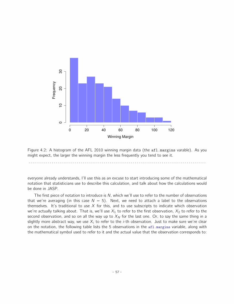
Winning Margin

Fre

qu

en

cy

0 20 40 60 80 100 120

01

02

03

0

Figure 4.2: A histogram of the AFL 2010 winning margin data (the afl.margins varable). As youmight expect, the larger the winning margin the less frequently you tend to see it.

. . . . . . . . . . . . . . . . . . . . . . . . . . . . . . . . . . . . . . . . . . . . . . . . . . . . . . . . . . . . . . . . . . . . . . . . . . . . . . . . . . . . . . . . . . . .

everyone already understands, I’ll use this as an excuse to start introducing some of the mathematicalnotation that statisticians use to describe this calculation, and talk about how the calculations wouldbe done in JASP.

The first piece of notation to introduce is N, which we’ll use to refer to the number of observationsthat we’re averaging (in this case N “ 5). Next, we need to attach a label to the observationsthemselves. It’s traditional to use X for this, and to use subscripts to indicate which observationwe’re actually talking about. That is, we’ll use X1 to refer to the first observation, X2 to refer to thesecond observation, and so on all the way up to XN for the last one. Or, to say the same thing in aslightly more abstract way, we use Xi to refer to the i-th observation. Just to make sure we’re clearon the notation, the following table lists the 5 observations in the afl.margins variable, along withthe mathematical symbol used to refer to it and the actual value that the observation corresponds to:

- 57 -

the observation its symbol the observed valuewinning margin, game 1 X1 56 pointswinning margin, game 2 X2 31 pointswinning margin, game 3 X3 56 pointswinning margin, game 4 X4 8 pointswinning margin, game 5 X5 32 points

Okay, now let’s try to write a formula for the mean. By tradition, we use X as the notation for themean. So the calculation for the mean could be expressed using the following formula:

X “X1 `X2 ` . . .`XN´1 `XN

N

This formula is entirely correct but it’s terribly long, so we make use of the summation symbol ř

to shorten it.a If I want to add up the first five observations I could write out the sum the long way,X1 `X2 `X3 `X4 `X5 or I could use the summation symbol to shorten it to this:

5ÿ

i“1

Xi

Taken literally, this could be read as “the sum, taken over all i values from 1 to 5, of the value Xi ”.But basically what it means is “add up the first five observations”. In any case, we can use thisnotation to write out the formula for the mean, which looks like this:

X “1

N

Nÿ

i“1

Xi

In all honesty, I can’t imagine that all this mathematical notation helps clarify the concept ofthe mean at all. In fact, it’s really just a fancy way of writing out the same thing I said in words:add all the values up and then divide by the total number of items. However, that’s not really thereason I went into all that detail. My goal was to try to make sure that everyone reading this bookis clear on the notation that we’ll be using throughout the book: X for the mean, ř for the idea ofsummation, Xi for the ith observation, and N for the total number of observations. We’re going tobe re-using these symbols a fair bit so it’s important that you understand them well enough to beable to “read” the equations, and to be able to see that it’s just saying “add up lots of things andthen divide by another thing”.

aThe choice to use Σ to denote summation isn’t arbitrary. It’s the Greek upper case letter sigma, which is theanalogue of the letter S in that alphabet. Similarly, there’s an equivalent symbol used to denote the multiplication oflots of numbers, because multiplications are also called “products” we use the Π symbol for this (the Greek upper casepi, which is the analogue of the letter P).

- 58 -

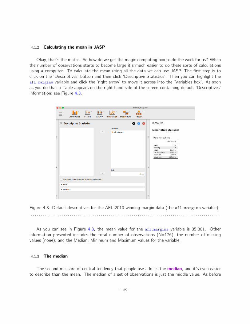
4.1.2 Calculating the mean in JASP

Okay, that’s the maths. So how do we get the magic computing box to do the work for us? Whenthe number of observations starts to become large it’s much easier to do these sorts of calculationsusing a computer. To calculate the mean using all the data we can use JASP. The first step is toclick on the ‘Descriptives’ button and then click ‘Descriptive Statistics’. Then you can highlight theafl.margins variable and click the ‘right arrow’ to move it across into the ‘Variables box’. As soonas you do that a Table appears on the right hand side of the screen containing default ‘Descriptives’information; see Figure 4.3.

Figure 4.3: Default descriptives for the AFL 2010 winning margin data (the afl.margins variable).

. . . . . . . . . . . . . . . . . . . . . . . . . . . . . . . . . . . . . . . . . . . . . . . . . . . . . . . . . . . . . . . . . . . . . . . . . . . . . . . . . . . . . . . . . . . .

As you can see in Figure 4.3, the mean value for the afl.margins variable is 35.301. Otherinformation presented includes the total number of observations (N=176), the number of missingvalues (none), and the Median, Minimum and Maximum values for the variable.

4.1.3 The median

The second measure of central tendency that people use a lot is the median, and it’s even easierto describe than the mean. The median of a set of observations is just the middle value. As before

- 59 -

let’s imagine we were interested only in the first 5 AFL winning margins: 56, 31, 56, 8 and 32. Tofigure out the median we sort these numbers into ascending order:

8, 31, 32, 56, 56

From inspection, it’s obvious that the median value of these 5 observations is 32 since that’s themiddle one in the sorted list (I’ve put it in bold to make it even more obvious). Easy stuff. But whatshould we do if we are interested in the first 6 games rather than the first 5? Since the sixth game inthe season had a winning margin of 14 points, our sorted list is now

8, 14, 31, 32, 56, 56

and there are two middle numbers, 31 and 32. The median is defined as the average of those twonumbers, which is of course 31.5. As before, it’s very tedious to do this by hand when you’ve got lotsof numbers. In real life, of course, no-one actually calculates the median by sorting the data and thenlooking for the middle value. In real life we use a computer to do the heavy lifting for us. JASP willgive us the median if we ask for it; we simply need to click on the ’Statistics’ dropdown menu andselect ’Median’ from the ’Central Tendency’ menu. The results will automatically update to includethis median, which JASP reports as 30.500 for the afl.margins variable.

4.1.4 Mean or median? What’s the difference?

Knowing how to calculate means and medians is only a part of the story. You also need tounderstand what each one is saying about the data, and what that implies for when you should useeach one. This is illustrated in Figure 4.4. The mean is kind of like the “centre of gravity” of the dataset, whereas the median is the “middle value” in the data. What this implies, as far as which one youshould use, depends a little on what type of data you’ve got and what you’re trying to achieve. As arough guide:

• If your data are nominal scale you probably shouldn’t be using either the mean or the median.Both the mean and the median rely on the idea that the numbers assigned to values are meaning-ful. If the numbering scheme is arbitrary then it’s probably best to use the mode (Section 4.1.6)instead.

• If your data are ordinal scale you’re more likely to want to use the median than the mean. Themedian only makes use of the order information in your data (i.e., which numbers are bigger) butdoesn’t depend on the precise numbers involved. That’s exactly the situation that applies whenyour data are ordinal scale. The mean, on the other hand, makes use of the precise numericvalues assigned to the observations, so it’s not really appropriate for ordinal data.

• For interval and ratio scale data either one is generally acceptable. Which one you pick depends abit on what you’re trying to achieve. The mean has the advantage that it uses all the informationin the data (which is useful when you don’t have a lot of data). But it’s very sensitive to extreme,outlying values.

- 60 -

Figure 4.4: An illustration of the difference between how the mean and the median should be inter-preted. The mean is basically the “centre of gravity” of the data set. If you imagine that the histogramof the data is a solid object, then the point on which you could balance it (as if on a see-saw) is themean. In contrast, the median is the middle observation, with half of the observations smaller andhalf of the observations larger.

. . . . . . . . . . . . . . . . . . . . . . . . . . . . . . . . . . . . . . . . . . . . . . . . . . . . . . . . . . . . . . . . . . . . . . . . . . . . . . . . . . . . . . . . . . . .

Let’s expand on that last part a little. One consequence is that there are systematic differencesbetween the mean and the median when the histogram is asymmetric (skewed; see Section 4.3). Thisis illustrated in Figure 4.4. Notice that the median (right hand side) is located closer to the “body” ofthe histogram, whereas the mean (left hand side) gets dragged towards the “tail” (where the extremevalues are). To give a concrete example, suppose Bob (income $50,000), Kate (income $60,000)and Jane (income $65,000) are sitting at a table. The average income at the table is $58,333 andthe median income is $60,000. Then Bill sits down with them (income $100,000,000). The averageincome has now jumped to $25,043,750 but the median rises only to $62,500. If you’re interested inlooking at the overall income at the table the mean might be the right answer. But if you’re interestedin what counts as a typical income at the table the median would be a better choice here.

4.1.5 A real life example

To try to get a sense of why you need to pay attention to the differences between the mean andthe median let’s consider a real life example. Since I tend to mock journalists for their poor scientificand statistical knowledge, I should give credit where credit is due. This is an excellent article on theABC news website2 from 24 September, 2010:

Senior Commonwealth Bank executives have travelled the world in the past couple of weeks witha presentation showing how Australian house prices, and the key price to income ratios, compare

2www.abc.net.au/news/stories/2010/09/24/3021480.htm

- 61 -

www.abc.net.au/news/stories/2010/09/24/3021480.htm

favourably with similar countries. “Housing affordability has actually been going sideways for thelast five to six years,” said Craig James, the chief economist of the bank’s trading arm, CommSec.

This probably comes as a huge surprise to anyone with a mortgage, or who wants a mortgage, or paysrent, or isn’t completely oblivious to what’s been going on in the Australian housing market over thelast several years. Back to the article:

CBA has waged its war against what it believes are housing doomsayers with graphs, numbers andinternational comparisons. In its presentation, the bank rejects arguments that Australia’s housingis relatively expensive compared to incomes. It says Australia’s house price to household incomeratio of 5.6 in the major cities, and 4.3 nationwide, is comparable to many other developed nations.It says San Francisco and New York have ratios of 7, Auckland’s is 6.7, and Vancouver comes inat 9.3.

More excellent news! Except, the article goes on to make the observation that:

Many analysts say that has led the bank to use misleading figures and comparisons. If you go to pagefour of CBA’s presentation and read the source information at the bottom of the graph and table,you would notice there is an additional source on the international comparison – Demographia.However, if the Commonwealth Bank had also used Demographia’s analysis of Australia’s houseprice to income ratio, it would have come up with a figure closer to 9 rather than 5.6 or 4.3

That’s, um, a rather serious discrepancy. One group of people say 9, another says 4-5. Should we justsplit the difference and say the truth lies somewhere in between? Absolutely not! This is a situationwhere there is a right answer and a wrong answer. Demographia is correct, and the CommonwealthBank is wrong. As the article points out:

[An] obvious problem with the Commonwealth Bank’s domestic price to income figures is theycompare average incomes with median house prices (unlike the Demographia figures that comparemedian incomes to median prices). The median is the mid-point, effectively cutting out the highsand lows, and that means the average is generally higher when it comes to incomes and assetprices, because it includes the earnings of Australia’s wealthiest people. To put it another way: theCommonwealth Bank’s figures count Ralph Norris’ multi-million dollar pay packet on the incomeside, but not his (no doubt) very expensive house in the property price figures, thus understatingthe house price to income ratio for middle-income Australians.

Couldn’t have put it better myself. The way that Demographia calculated the ratio is the right thingto do. The way that the Bank did it is incorrect. As for why an extremely quantitatively sophisticatedorganisation such as a major bank made such an elementary mistake, well... I can’t say for sure since Ihave no special insight into their thinking. But the article itself does happen to mention the followingfacts, which may or may not be relevant:

[As] Australia’s largest home lender, the Commonwealth Bank has one of the biggest vestedinterests in house prices rising. It effectively owns a massive swathe of Australian housing assecurity for its home loans as well as many small business loans.

My, my.

- 62 -

4.1.6 Mode

The mode of a sample is very simple. It is the value that occurs most frequently. We canillustrate the mode using a different AFL variable: who has played in the most finals? Open theaflsmall_finalists file and take a look at the afl.finalists variable, see Figure 4.5. This variablecontains the names of all 400 teams that played in all 200 finals matches played during the period1987 to 2010.

Figure 4.5: A screenshot of JASP showing the variables stored in the aflsmall_finalists.csv file

. . . . . . . . . . . . . . . . . . . . . . . . . . . . . . . . . . . . . . . . . . . . . . . . . . . . . . . . . . . . . . . . . . . . . . . . . . . . . . . . . . . . . . . . . . . .

What we could do is read through all 400 entries and count the number of occasions on whicheach team name appears in our list of finalists, thereby producing a frequency table. However, thatwould be mindless and boring: exactly the sort of task that computers are great at. So let’s use JASPto do this for us. Under ‘Descriptives’ - ‘Descriptive Statistics’, select the afl.finalists variable andmove it to the ’Variables’ box, then click the small check box labelled ‘Frequency tables’. You shouldget something like Figure 4.6.

Now that we have our frequency table we can just look at it and see that, over the 24 years forwhich we have data, Geelong has played in more finals than any other team. Thus, the mode of theafl.finalists data is "Geelong". We can see that Geelong (39 finals) played in more finals than anyother team during the 1987-2010 period. It’s also worth noting that in the ‘Descriptives’ Table noresults are calculated for Mean, Median, Minimum or Maximum. This is because the afl.finalistsvariable is a nominal text variable so it makes no sense to calculate these values.

One last point to make regarding the mode. Whilst the mode is most often calculated when youhave nominal data, because means and medians are useless for those sorts of variables, there are somesituations in which you really do want to know the mode of an ordinal, interval or ratio scale variable.

- 63 -

Figure 4.6: A screenshot of JASP showing the frequency table for the afl.finalists variable

. . . . . . . . . . . . . . . . . . . . . . . . . . . . . . . . . . . . . . . . . . . . . . . . . . . . . . . . . . . . . . . . . . . . . . . . . . . . . . . . . . . . . . . . . . . .

- 64 -

For instance, let’s go back to our afl.margins variable. This variable is clearly ratio scale (if it’s notclear to you, it may help to re-read Section 2.2), and so in most situations the mean or the medianis the measure of central tendency that you want. But consider this scenario: a friend of yours isoffering a bet and they pick a football game at random. Without knowing who is playing you have toguess the exact winning margin. If you guess correctly you win $50. If you don’t you lose $1. Thereare no consolation prizes for “almost” getting the right answer. You have to guess exactly the rightmargin. For this bet, the mean and the median are completely useless to you. It is the mode thatyou should bet on. To calculate the mode for the afl.margins variable in JASP, go back to that dataset and on the ‘Descriptives’ - ‘Descriptive Statistics’ screen you will see you can expand the sectionmarked ‘Statistics’. Click on the checkbox marked ‘Mode’ and you will see the modal value presentedin the ‘Descriptive Statistics’ Table, as in Figure 4.7. So the 2010 data suggest you should bet on a3 point margin.

Figure 4.7: A screenshot of JASP showing the modal value for the afl.margins variable

. . . . . . . . . . . . . . . . . . . . . . . . . . . . . . . . . . . . . . . . . . . . . . . . . . . . . . . . . . . . . . . . . . . . . . . . . . . . . . . . . . . . . . . . . . . .

- 65 -

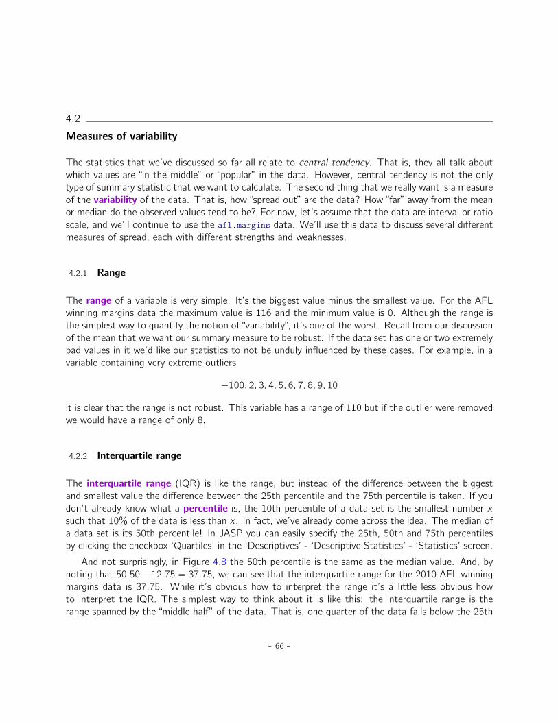
4.2

Measures of variability

The statistics that we’ve discussed so far all relate to central tendency. That is, they all talk aboutwhich values are “in the middle” or “popular” in the data. However, central tendency is not the onlytype of summary statistic that we want to calculate. The second thing that we really want is a measureof the variability of the data. That is, how “spread out” are the data? How “far” away from the meanor median do the observed values tend to be? For now, let’s assume that the data are interval or ratioscale, and we’ll continue to use the afl.margins data. We’ll use this data to discuss several differentmeasures of spread, each with different strengths and weaknesses.

4.2.1 Range

The range of a variable is very simple. It’s the biggest value minus the smallest value. For the AFLwinning margins data the maximum value is 116 and the minimum value is 0. Although the range isthe simplest way to quantify the notion of “variability”, it’s one of the worst. Recall from our discussionof the mean that we want our summary measure to be robust. If the data set has one or two extremelybad values in it we’d like our statistics to not be unduly influenced by these cases. For example, in avariable containing very extreme outliers

´100, 2, 3, 4, 5, 6, 7, 8, 9, 10

it is clear that the range is not robust. This variable has a range of 110 but if the outlier were removedwe would have a range of only 8.

4.2.2 Interquartile range

The interquartile range (IQR) is like the range, but instead of the difference between the biggestand smallest value the difference between the 25th percentile and the 75th percentile is taken. If youdon’t already know what a percentile is, the 10th percentile of a data set is the smallest number xsuch that 10% of the data is less than x . In fact, we’ve already come across the idea. The median ofa data set is its 50th percentile! In JASP you can easily specify the 25th, 50th and 75th percentilesby clicking the checkbox ‘Quartiles’ in the ‘Descriptives’ - ‘Descriptive Statistics’ - ‘Statistics’ screen.

And not surprisingly, in Figure 4.8 the 50th percentile is the same as the median value. And, bynoting that 50.50´ 12.75 “ 37.75, we can see that the interquartile range for the 2010 AFL winningmargins data is 37.75. While it’s obvious how to interpret the range it’s a little less obvious howto interpret the IQR. The simplest way to think about it is like this: the interquartile range is therange spanned by the “middle half” of the data. That is, one quarter of the data falls below the 25th

- 66 -

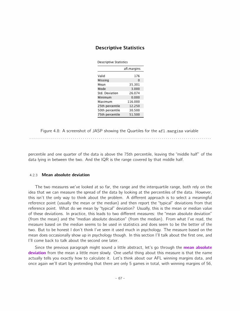
Figure 4.8: A screenshot of JASP showing the Quartiles for the afl.margins variable

. . . . . . . . . . . . . . . . . . . . . . . . . . . . . . . . . . . . . . . . . . . . . . . . . . . . . . . . . . . . . . . . . . . . . . . . . . . . . . . . . . . . . . . . . . . .

percentile and one quarter of the data is above the 75th percentile, leaving the “middle half” of thedata lying in between the two. And the IQR is the range covered by that middle half.

4.2.3 Mean absolute deviation

The two measures we’ve looked at so far, the range and the interquartile range, both rely on theidea that we can measure the spread of the data by looking at the percentiles of the data. However,this isn’t the only way to think about the problem. A different approach is to select a meaningfulreference point (usually the mean or the median) and then report the “typical” deviations from thatreference point. What do we mean by “typical” deviation? Usually, this is the mean or median valueof these deviations. In practice, this leads to two different measures: the “mean absolute deviation”(from the mean) and the “median absolute deviation” (from the median). From what I’ve read, themeasure based on the median seems to be used in statistics and does seem to be the better of thetwo. But to be honest I don’t think I’ve seen it used much in psychology. The measure based on themean does occasionally show up in psychology though. In this section I’ll talk about the first one, andI’ll come back to talk about the second one later.

Since the previous paragraph might sound a little abstract, let’s go through the mean absolutedeviation from the mean a little more slowly. One useful thing about this measure is that the nameactually tells you exactly how to calculate it. Let’s think about our AFL winning margins data, andonce again we’ll start by pretending that there are only 5 games in total, with winning margins of 56,

- 67 -

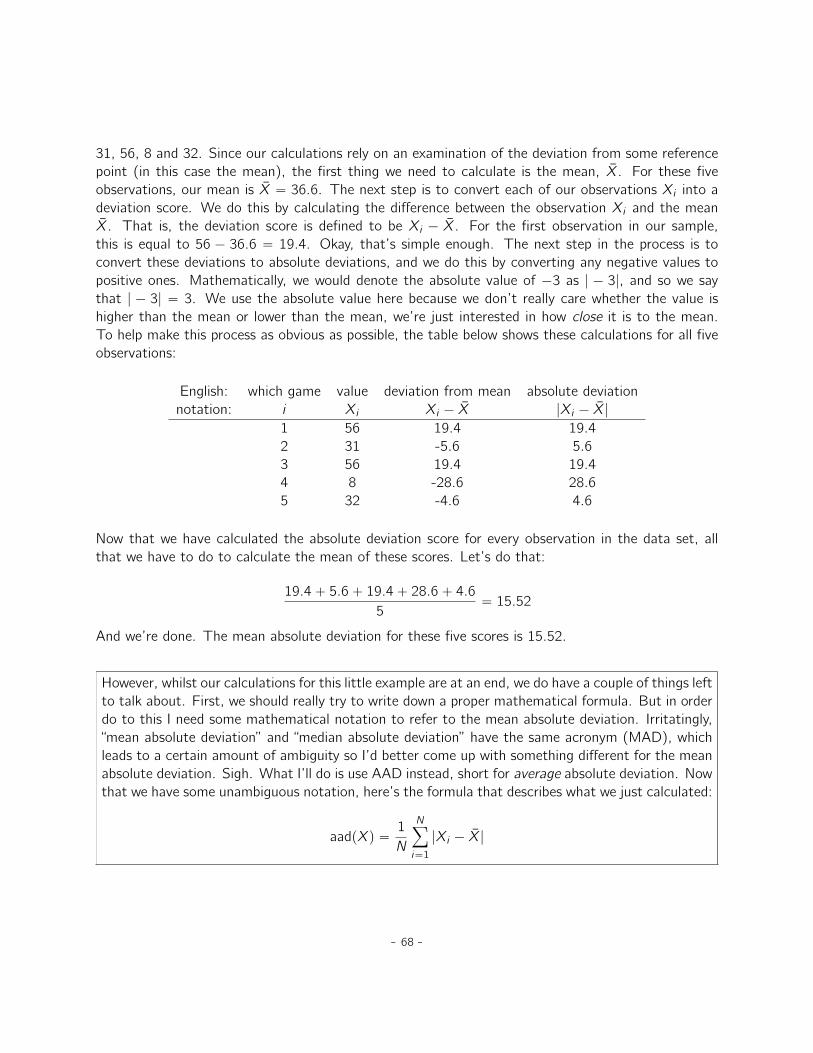
31, 56, 8 and 32. Since our calculations rely on an examination of the deviation from some referencepoint (in this case the mean), the first thing we need to calculate is the mean, X. For these fiveobservations, our mean is X “ 36.6. The next step is to convert each of our observations Xi into adeviation score. We do this by calculating the difference between the observation Xi and the meanX. That is, the deviation score is defined to be Xi ´ X. For the first observation in our sample,this is equal to 56 ´ 36.6 “ 19.4. Okay, that’s simple enough. The next step in the process is toconvert these deviations to absolute deviations, and we do this by converting any negative values topositive ones. Mathematically, we would denote the absolute value of ´3 as | ´ 3|, and so we saythat | ´ 3| “ 3. We use the absolute value here because we don’t really care whether the value ishigher than the mean or lower than the mean, we’re just interested in how close it is to the mean.To help make this process as obvious as possible, the table below shows these calculations for all fiveobservations:

English: which game value deviation from mean absolute deviationnotation: i Xi Xi ´ X |Xi ´ X|

1 56 19.4 19.42 31 -5.6 5.63 56 19.4 19.44 8 -28.6 28.65 32 -4.6 4.6

Now that we have calculated the absolute deviation score for every observation in the data set, allthat we have to do to calculate the mean of these scores. Let’s do that:

19.4` 5.6` 19.4` 28.6` 4.6

5“ 15.52

And we’re done. The mean absolute deviation for these five scores is 15.52.

However, whilst our calculations for this little example are at an end, we do have a couple of things leftto talk about. First, we should really try to write down a proper mathematical formula. But in orderdo to this I need some mathematical notation to refer to the mean absolute deviation. Irritatingly,“mean absolute deviation” and “median absolute deviation” have the same acronym (MAD), whichleads to a certain amount of ambiguity so I’d better come up with something different for the meanabsolute deviation. Sigh. What I’ll do is use AAD instead, short for average absolute deviation. Nowthat we have some unambiguous notation, here’s the formula that describes what we just calculated:

aadpXq “1

N

Nÿ

i“1

|Xi ´ X|

- 68 -

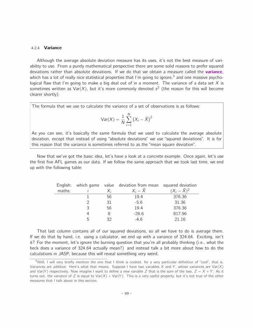
4.2.4 Variance

Although the average absolute deviation measure has its uses, it’s not the best measure of vari-ability to use. From a purely mathematical perspective there are some solid reasons to prefer squareddeviations rather than absolute deviations. If we do that we obtain a measure called the variance,which has a lot of really nice statistical properties that I’m going to ignore,3 and one massive psycho-logical flaw that I’m going to make a big deal out of in a moment. The variance of a data set X issometimes written as VarpXq, but it’s more commonly denoted s2 (the reason for this will becomeclearer shortly).

The formula that we use to calculate the variance of a set of observations is as follows:

VarpXq “1

N

Nÿ

i“1

`

Xi ´ X˘2

As you can see, it’s basically the same formula that we used to calculate the average absolutedeviation, except that instead of using “absolute deviations” we use “squared deviations”. It is forthis reason that the variance is sometimes referred to as the “mean square deviation”.

Now that we’ve got the basic idea, let’s have a look at a concrete example. Once again, let’s usethe first five AFL games as our data. If we follow the same approach that we took last time, we endup with the following table:

English: which game value deviation from mean squared deviationmaths: i Xi Xi ´ X pXi ´ Xq

2

1 56 19.4 376.362 31 -5.6 31.363 56 19.4 376.364 8 -28.6 817.965 32 -4.6 21.16

That last column contains all of our squared deviations, so all we have to do is average them.If we do that by hand, i.e. using a calculator, we end up with a variance of 324.64. Exciting, isn’tit? For the moment, let’s ignore the burning question that you’re all probably thinking (i.e., what theheck does a variance of 324.64 actually mean?) and instead talk a bit more about how to do thecalculations in JASP, because this will reveal something very weird.

3Well, I will very briefly mention the one that I think is coolest, for a very particular definition of “cool”, that is.Variances are additive. Here’s what that means. Suppose I have two variables X and Y , whose variances are VarpXqand VarpY q respectively. Now imagine I want to define a new variable Z that is the sum of the two, Z “ X ` Y . As itturns out, the variance of Z is equal to VarpXq ` VarpY q. This is a very useful property, but it’s not true of the othermeasures that I talk about in this section.

- 69 -

First, you’ll need to load a new data file that contains only the first 5 rows. Do to this, load thefile aflsmall_margins_first5.csv. Next, click ‘Descriptives’ – ’Descriptive Statistics’, and thenunder the ’Statistics’ menu, click the ‘Variance’ check box (you’ll find it in the ’Dispersion’ group. Doyou get the same values for variance as the one we calculated by hand (324.64)? No, wait, you geta completely different answer (405.800)! That’s just weird. Is JASP broken? Is this a typo? What isgoing on?

As it happens, the answer is no. It’s not a typo, and JASP is not making a mistake. In fact, it’svery simple to explain what JASP is doing here, but slightly trickier to explain why JASP is doing it.So let’s start with the “what”. What JASP is doing is evaluating a slightly different formula to theone I showed you above. Instead of averaging the squared deviations, which requires you to divide bythe number of data points N, JASP has chosen to divide by N ´ 1.

In other words, the formula that JASP is using is this one:

1

N ´ 1

Nÿ

i“1

`

Xi ´ X˘2

So that’s the what. The real question is why JASP is dividing by N ´ 1 and not by N. After all,the variance is supposed to be the mean squared deviation, right? So shouldn’t we be dividing by N,the actual number of observations in the sample? Well, yes, we should. However, as we’ll discuss inChapter 7, there’s a subtle distinction between “describing a sample” and “making guesses about thepopulation from which the sample came”. Up to this point, it’s been a distinction without a difference.Regardless of whether you’re describing a sample or drawing inferences about the population, themean is calculated exactly the same way. Not so for the variance, or the standard deviation, or formany other measures besides. What I outlined to you initially (i.e., take the actual average, and thusdivide by N) assumes that you literally intend to calculate the variance of the sample. Most of thetime, however, you’re not terribly interested in the sample in and of itself. Rather, the sample existsto tell you something about the world. If so, you’re actually starting to move away from calculating a“sample statistic” and towards the idea of estimating a “population parameter”. However, I’m gettingahead of myself. For now, let’s just take it on faith that JASP knows what it’s doing, and we’ll revisitthe question later on when we talk about estimation in Chapter 7.

Okay, one last thing. This section so far has read a bit like a mystery novel. I’ve shown you howto calculate the variance, described the weird “N ´ 1” thing that JASP does and hinted at the reasonwhy it’s there, but I haven’t mentioned the single most important thing. How do you interpret thevariance? Descriptive statistics are supposed to describe things, after all, and right now the varianceis really just a gibberish number. Unfortunately, the reason why I haven’t given you the human-friendlyinterpretation of the variance is that there really isn’t one. This is the most serious problem withthe variance. Although it has some elegant mathematical properties that suggest that it really isa fundamental quantity for expressing variation, it’s completely useless if you want to communicatewith an actual human. Variances are completely uninterpretable in terms of the original variable! Allthe numbers have been squared and they don’t mean anything anymore. This is a huge issue. For

- 70 -

instance, according to the table I presented earlier, the margin in game 1 was “376.36 points-squaredhigher than the average margin”. This is exactly as stupid as it sounds, and so when we calculatea variance of 324.64 we’re in the same situation. I’ve watched a lot of football games, and at notime has anyone ever referred to “points squared”. It’s not a real unit of measurement, and since thevariance is expressed in terms of this gibberish unit, it is totally meaningless to a human.

4.2.5 Standard deviation

Okay, suppose that you like the idea of using the variance because of those nice mathematicalproperties that I haven’t talked about, but since you’re a human and not a robot you’d like to have ameasure that is expressed in the same units as the data itself (i.e., points, not points-squared). Whatshould you do? The solution to the problem is obvious! Take the square root of the variance, knownas the standard deviation, also called the “root mean squared deviation”, or RMSD. This solves ourproblem fairly neatly. Whilst nobody has a clue what “a variance of 324.68 points-squared” reallymeans, it’s much easier to understand “a standard deviation of 18.01 points” since it’s expressed inthe original units. It is traditional to refer to the standard deviation of a sample of data as s, though“sd” and “std dev.” are also used at times.

Because the standard deviation is equal to the square root of the variance, you probably won’t besurprised to see that the formula is:

s “

g

f

f

e

1

N

Nÿ

i“1

`

Xi ´ X˘2

and in JASP there is a check box for ‘Std. deviation’ in the same section as the check box for‘Variance’. As you can see in Figure 4.8, the value JASP gives for the standard deviation ofafl.margins is 26.074. Note that because standard deviation is used so often, it is checked bydefault, so you will rarely have to actually select it yourself!

However, as you might have guessed from our discussion of the variance, what JASP actuallycalculates is slightly different to the formula given above. Just like the we saw with the variance, whatJASP calculates is a version that divides by N ´ 1 rather than N.

For reasons that will make sense when we return to this topic in Chapter 7 I’ll refer to this newquantity as σ (read as: “sigma hat”), and the formula for this is:

σ “

g

f

f

e

1

N ´ 1

Nÿ

i“1

`

Xi ´ X˘2

Interpreting standard deviations is slightly more complex. Because the standard deviation is derived

- 71 -

from the variance, and the variance is a quantity that has little to no meaning that makes sense tous humans, the standard deviation doesn’t have a simple interpretation. As a consequence, most ofus just rely on a simple rule of thumb. In general, you should expect 68% of the data to fall within 1standard deviation of the mean, 95% of the data to fall within 2 standard deviation of the mean, and99.7% of the data to fall within 3 standard deviations of the mean. This rule tends to work prettywell most of the time, but it’s not exact. It’s actually calculated based on an assumption that thehistogram is symmetric and “bell shaped”.4 As you can tell from looking at the AFL winning marginshistogram in Figure 4.2, this isn’t exactly true of our data! Even so, the rule is approximately correct.As it turns out, 65.3% of the AFL margins data fall within one standard deviation of the mean. Thisis shown visually in Figure 4.9.

Mean − SD Mean Mean + SD

Figure 4.9: An illustration of the standard deviation from the AFL winning margins data. The shadedbars in the histogram show how much of the data fall within one standard deviation of the mean. In thiscase, 65.3% of the data set lies within this range, which is pretty consistent with the “approximately68% rule” discussed in the main text.

. . . . . . . . . . . . . . . . . . . . . . . . . . . . . . . . . . . . . . . . . . . . . . . . . . . . . . . . . . . . . . . . . . . . . . . . . . . . . . . . . . . . . . . . . . . .

4.2.6 Which measure to use?

We’ve discussed quite a few measures of spread: range, IQR, mean absolute deviation, varianceand standard deviation; and hinted at their strengths and weaknesses. Here’s a quick summary:

4Strictly, the assumption is that the data are normally distributed, which is an important concept that we’ll discussmore in Chapter 6 and will turn up over and over again later in the book.

- 72 -

• Range. Gives you the full spread of the data. It’s very vulnerable to outliers and as a consequenceit isn’t often used unless you have good reasons to care about the extremes in the data.

• Interquartile range. Tells you where the “middle half” of the data sits. It’s pretty robust andcomplements the median nicely. This is used a lot.

• Mean absolute deviation. Tells you how far “on average” the observations are from the mean.It’s very interpretable but has a few minor issues (not discussed here) that make it less attractiveto statisticians than the standard deviation. Used sometimes, but not often.

• Variance. Tells you the average squared deviation from the mean. It’s mathematically elegantand is probably the “right” way to describe variation around the mean, but it’s completely unin-terpretable because it doesn’t use the same units as the data. Almost never used except as amathematical tool, but it’s buried “under the hood” of a very large number of statistical tools.

• Standard deviation. This is the square root of the variance. It’s fairly elegant mathematicallyand it’s expressed in the same units as the data so it can be interpreted pretty well. In situationswhere the mean is the measure of central tendency, this is the default. This is by far the mostpopular measure of variation.

In short, the IQR and the standard deviation are easily the two most common measures used to reportthe variability of the data. But there are situations in which the others are used. I’ve described all ofthem in this book because there’s a fair chance you’ll run into most of these somewhere.

4.3

Skew and kurtosis

There are two more descriptive statistics that you will sometimes see reported in the psychologicalliterature: skew and kurtosis. In practice, neither one is used anywhere near as frequently as themeasures of central tendency and variability that we’ve been talking about. Skew is pretty important,so you do see it mentioned a fair bit, but I’ve actually never seen kurtosis reported in a scientific articleto date.

Since it’s the more interesting of the two, let’s start by talking about the skewness. Skewness isbasically a measure of asymmetry and the easiest way to explain it is by drawing some pictures. AsFigure 4.10 illustrates, if the data tend to have a lot of extreme small values (i.e., the lower tail is“longer” than the upper tail) and not so many extremely large values (left panel) then we say that thedata are negatively skewed. On the other hand, if there are more extremely large values than extremelysmall ones (right panel) we say that the data are positively skewed. That’s the qualitative idea behindskewness. If there are relatively more values that are far greater than the mean, the distribution ispositively skewed or right skewed, with a tail stretching to the right. Negative or left skew is the

- 73 -

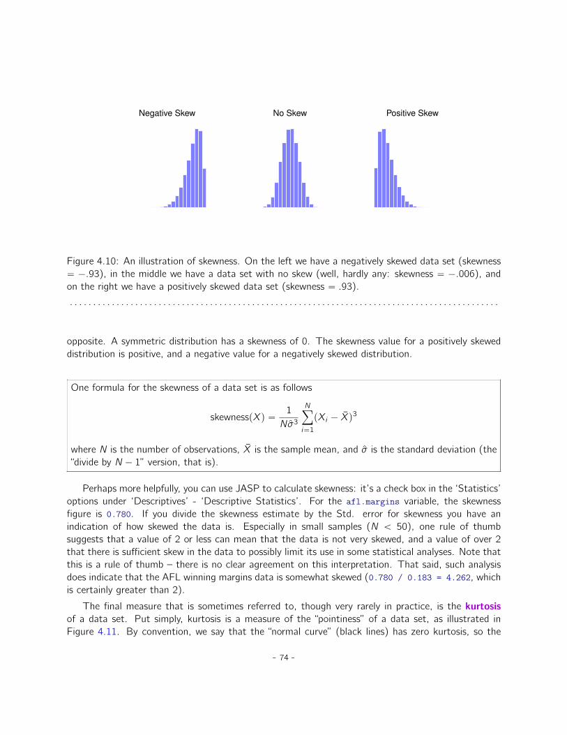
Negative Skew No Skew Positive Skew

Figure 4.10: An illustration of skewness. On the left we have a negatively skewed data set (skewness“ ´.93), in the middle we have a data set with no skew (well, hardly any: skewness “ ´.006), andon the right we have a positively skewed data set (skewness “ .93).

. . . . . . . . . . . . . . . . . . . . . . . . . . . . . . . . . . . . . . . . . . . . . . . . . . . . . . . . . . . . . . . . . . . . . . . . . . . . . . . . . . . . . . . . . . . .

opposite. A symmetric distribution has a skewness of 0. The skewness value for a positively skeweddistribution is positive, and a negative value for a negatively skewed distribution.

One formula for the skewness of a data set is as follows

skewnesspXq “1

Nσ3

Nÿ

i“1

pXi ´ Xq3

where N is the number of observations, X is the sample mean, and σ is the standard deviation (the“divide by N ´ 1” version, that is).

Perhaps more helpfully, you can use JASP to calculate skewness: it’s a check box in the ‘Statistics’options under ‘Descriptives’ - ‘Descriptive Statistics’. For the afl.margins variable, the skewnessfigure is 0.780. If you divide the skewness estimate by the Std. error for skewness you have anindication of how skewed the data is. Especially in small samples (N ă 50), one rule of thumbsuggests that a value of 2 or less can mean that the data is not very skewed, and a value of over 2that there is sufficient skew in the data to possibly limit its use in some statistical analyses. Note thatthis is a rule of thumb – there is no clear agreement on this interpretation. That said, such analysisdoes indicate that the AFL winning margins data is somewhat skewed (0.780 / 0.183 = 4.262, whichis certainly greater than 2).

The final measure that is sometimes referred to, though very rarely in practice, is the kurtosisof a data set. Put simply, kurtosis is a measure of the “pointiness” of a data set, as illustrated inFigure 4.11. By convention, we say that the “normal curve” (black lines) has zero kurtosis, so the

- 74 -

pointiness of a data set is assessed relative to this curve.

Platykurtic("too flat")

MesokurticLeptokurtic

("too pointy")

Figure 4.11: An illustration of kurtosis. On the left, we have a “platykurtic” data set (kurtosis =´.95) meaning that the data set is “too flat”. In the middle we have a “mesokurtic” data set (kurtosisis almost exactly 0) which means that the pointiness of the data is just about right. Finally, on theright, we have a “leptokurtic” data set (kurtosis “ 2.12) indicating that the data set is “too pointy”.Note that kurtosis is measured with respect to a normal curve (black line).

. . . . . . . . . . . . . . . . . . . . . . . . . . . . . . . . . . . . . . . . . . . . . . . . . . . . . . . . . . . . . . . . . . . . . . . . . . . . . . . . . . . . . . . . . . . .

In this Figure, the data on the left are not pointy enough, so the kurtosis is negative and we callthe data platykurtic. The data on the right are too pointy, so the kurtosis is positive and we saythat the data is leptokurtic. But the data in the middle are just pointy enough, so we say that it ismesokurtic and has kurtosis zero. This is summarised in the table below:

informal term technical name kurtosis value“too flat” platykurtic negative“just pointy enough” mesokurtic zero“too pointy” leptokurtic positive

The equation for kurtosis is pretty similar in spirit to the formulas we’ve seen already for the varianceand the skewness. Except that where the variance involved squared deviations and the skewnessinvolved cubed deviations, the kurtosis involves raising the deviations to the fourth power:a

kurtosispXq “1

Nσ4

Nÿ

i“1

`

Xi ´ X˘4´ 3.

aThe “´3” part is something that statisticians tack on to ensure that the normal curve has kurtosis zero. It looksa bit silly, just sticking a “-3” at the end of the formula, but there are good mathematical reasons for doing this.

- 75 -

More to the point, JASP has a check box for kurtosis just below the check box for skewness, andthis gives a value for kurtosis of 0.101 with a standard error of 0.364. Using the same idea as beforewhere we divide the kurtosis by the standard error of the kurtosis, we note that this value is muchless than 2 (0.101/0.364 = 0.277). This means that the AFL winning margins data are just pointyenough.

4.4

Descriptive statistics separately for each group

It is very commonly the case that you find yourself needing to look at descriptive statistics broken downby some grouping variable. This is pretty easy to do in JASP. For instance, let’s say I want to lookat the descriptive statistics for some clin.trial data, broken down separately by therapy type. Thisis a new data set, one that you’ve never seen before. The data is stored in the clinicaltrial.csvfile and we’ll use it a lot in Chapter 12 (you can find a complete description of the data at the startof that chapter). Let’s load it and see what we’ve got:

Evidently there were three drugs: a placebo, something called “anxifree” and something called“joyzepam”, and there were 6 people administered each drug. There were 9 people treated usingcognitive behavioural therapy (CBT) and 9 people who received no psychological treatment. And wecan see from looking at the ‘Descriptives’ of the mood.gain variable that most people did show a moodgain (mean “ 0.88), though without knowing what the scale is here it’s hard to say much more thanthat. Still, that’s not too bad. Overall I feel that I learned something from that.

We can also go ahead and look at some other descriptive statistics, and this time separately foreach type of therapy. In JASP, check Std. deviation, Skewness, and Kurtosis in the ‘Statistics’ options.At the same time, transfer the therapy variable into the ‘Split’ box, and you should get somethinglike Figure 4.13

4.5

Standard scores

Suppose my friend is putting together a new questionnaire intended to measure “grumpiness”. Thesurvey has 50 questions which you can answer in a grumpy way or not. Across a big sample (hypo-thetically, let’s imagine a million people or so!) the data are fairly normally distributed, with the meangrumpiness score being 17 out of 50 questions answered in a grumpy way, and the standard deviationis 5. In contrast, when I take the questionnaire I answer 35 out of 50 questions in a grumpy way. So,how grumpy am I? One way to think about it would be to say that I have grumpiness of 35/50, so

- 76 -

you might say that I’m 70% grumpy. But that’s a bit weird, when you think about it. If my friendhad phrased her questions a bit differently people might have answered them in a different way, so theoverall distribution of answers could easily move up or down depending on the precise way in whichthe questions were asked. So, I’m only 70% grumpy with respect to this set of survey questions. Evenif it’s a very good questionnaire this isn’t very a informative statement.

A simpler way around this is to describe my grumpiness by comparing me to other people. Shock-ingly, out of my friend’s sample of 1,000,000 people, only 159 people were as grumpy as me (that’snot at all unrealistic, frankly) suggesting that I’m in the top 0.016% of people for grumpiness. Thismakes much more sense than trying to interpret the raw data. This idea, that we should describemy grumpiness in terms of the overall distribution of the grumpiness of humans, is the qualitativeidea that standardisation attempts to get at. One way to do this is to do exactly what I just did anddescribe everything in terms of percentiles. However, the problem with doing this is that “it’s lonelyat the top”. Suppose that my friend had only collected a sample of 1000 people (still a pretty bigsample for the purposes of testing a new questionnaire, I’d like to add), and this time gotten, let’ssay, a mean of 16 out of 50 with a standard deviation of 5. The problem is that almost certainly nota single person in that sample would be as grumpy as me.

However, all is not lost. A different approach is to convert my grumpiness score into a standardscore, also referred to as a z-score. The standard score is defined as the number of standard deviationsabove the mean that my grumpiness score lies. To phrase it in “pseudo-maths” the standard score iscalculated like this:

standard score “raw score´meanstandard deviation

In actual maths, the equation for the z-score is

zi “Xi ´ X

σ

So, going back to the grumpiness data, we can now transform Dani’s raw grumpiness into astandardised grumpiness score.

z “35´ 17

5“ 3.6

To interpret this value, recall the rough heuristic that I provided in Section 4.2.5 in which I notedthat 99.7% of values are expected to lie within 3 standard deviations of the mean. So the fact thatmy grumpiness corresponds to a z score of 3.6 indicates that I’m very grumpy indeed. In fact thissuggests that I’m grumpier than 99.98% of people. Sounds about right.

In addition to allowing you to interpret a raw score in relation to a larger population (and therebyallowing you to make sense of variables that lie on arbitrary scales), standard scores serve a seconduseful function. Standard scores can be compared to one another in situations where the raw scorescan’t. Suppose, for instance, my friend also had another questionnaire that measured extraversionusing a 24 item questionnaire. The overall mean for this measure turns out to be 13 with standard

- 77 -

deviation 4, and I scored a 2. As you can imagine, it doesn’t make a lot of sense to try to compare myraw score of 2 on the extraversion questionnaire to my raw score of 35 on the grumpiness questionnaire.The raw scores for the two variables are “about” fundamentally different things, so this would be likecomparing apples to oranges.

What about the standard scores? Well, this is a little different. If we calculate the standard scoreswe get z “ p35´17q{5 “ 3.6 for grumpiness and z “ p2´13q{4 “ ´2.75 for extraversion. These twonumbers can be compared to each other.5 I’m much less extraverted than most people (z “ ´2.75)and much grumpier than most people (z “ 3.6). But the extent of my unusualness is much moreextreme for grumpiness, since 3.6 is a bigger number than 2.75. Because each standardised score isa statement about where an observation falls relative to its own population, it is possible to comparestandardised scores across completely different variables.

4.6

Summary

Calculating some basic descriptive statistics is one of the very first things you do when analysing realdata, and descriptive statistics are much simpler to understand than inferential statistics, so like everyother statistics textbook I’ve started with descriptives. In this chapter, we talked about the followingtopics:

• Measures of central tendency. Broadly speaking, central tendency measures tell you where thedata are. There’s three measures that are typically reported in the literature: the mean, medianand mode. (Section 4.1)

• Measures of variability. In contrast, measures of variability tell you about how “spread out” thedata are. The key measures are: range, standard deviation, and interquartile range. (Section 4.2)

• Measures of skewness and kurtosis. We also looked at assymetry in a variable’s distribution(skew) and pointness (kurtosis). (Section 4.3)

• Getting group summaries of variables in JASP. Since this book focuses on doing data analysis inJASP, we spent a bit of time talking about how descriptive statistics are computed for differentsubgroups. (Section 4.4)

• Standard scores. The z-score is a slightly unusual beast. It’s not quite a descriptive statistic,and not quite an inference. We talked about it in Section 4.5. Make sure you understand thatsection. It’ll come up again later.

5Though some caution is usually warranted. It’s not always the case that one standard deviation on variable Acorresponds to the same “kind” of thing as one standard deviation on variable B. Use common sense when trying todetermine whether or not the z scores of two variables can be meaningfully compared.

- 78 -

In the next Chapter we’ll move on to a discussion of how to draw pictures! Everyone loves a prettypicture, right? But before we do, I want to end on an important point. A traditional first coursein statistics spends only a small proportion of the class on descriptive statistics, maybe one or twolectures at most. The vast majority of the lecturer’s time is spent on inferential statistics becausethat’s where all the hard stuff is. That makes sense, but it hides the practical everyday importance ofchoosing good descriptives. With that in mind. . .

4.6.1 Epilogue: Good descriptive statistics are descriptive!

The death of one man is a tragedy.The death of millions is a statistic.

– Josef Stalin, Potsdam 1945

950,000 – 1,200,000– Estimate of Soviet repression deaths,1937-1938 (Ellman 2002)

Stalin’s infamous quote about the statistical character of the deaths of millions is worth giving somethought. The clear intent of his statement is that the death of an individual touches us personallyand its force cannot be denied, but that the deaths of a multitude are incomprehensible and as aconsequence are mere statistics and more easily ignored. I’d argue that Stalin was half right. Astatistic is an abstraction, a description of events beyond our personal experience, and so hard tovisualise. Few if any of us can imagine what the deaths of millions is “really” like, but we can imagineone death and this gives the lone death its feeling of immediate tragedy, a feeling that is missing fromEllman’s cold statistical description.

Yet it is not so simple. Without numbers, without counts, without a description of what happened,we have no chance of understanding what really happened, no opportunity even to try to summon themissing feeling. And in truth, as I write this sitting in comfort on a Saturday morning half a worldand a whole lifetime away from the Gulags, when I put the Ellman estimate next to the Stalin quotea dull dread settles in my stomach and a chill settles over me. The Stalinist repression is somethingtruly beyond my experience, but with a combination of statistical data and those recorded personalhistories that have come down to us, it is not entirely beyond my comprehension. Because whatEllman’s numbers tell us is this: over a two year period Stalinist repression wiped out the equivalentof every man, woman and child currently alive in the city where I live. Each one of those deaths hadit’s own story, was it’s own tragedy, and only some of those are known to us now. Even so, with afew carefully chosen statistics, the scale of the atrocity starts to come into focus.

Thus it is no small thing to say that the first task of the statistician and the scientist is to summarisethe data, to find some collection of numbers that can convey to an audience a sense of what hashappened. This is the job of descriptive statistics, but it’s not a job that can be told solely using thenumbers. You are a data analyst, and not a statistical software package. Part of your job is to takethese statistics and turn them into a description. When you analyse data it is not sufficient to list off

- 79 -

a collection of numbers. Always remember that what you’re really trying to do is communicate witha human audience. The numbers are important, but they need to be put together into a meaningfulstory that your audience can interpret. That means you need to think about framing. You needto think about context. And you need to think about the individual events that your statistics aresummarising.

- 80 -

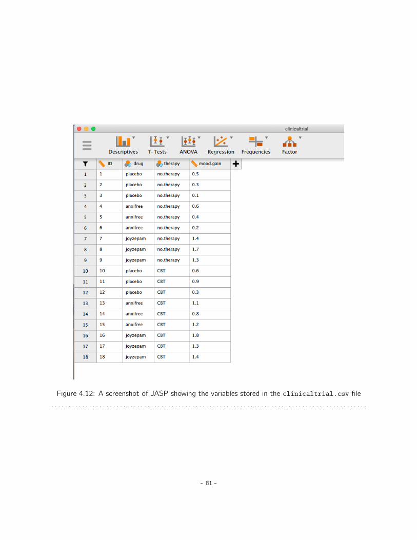
Figure 4.12: A screenshot of JASP showing the variables stored in the clinicaltrial.csv file

. . . . . . . . . . . . . . . . . . . . . . . . . . . . . . . . . . . . . . . . . . . . . . . . . . . . . . . . . . . . . . . . . . . . . . . . . . . . . . . . . . . . . . . . . . . .

- 81 -

Figure 4.13: A screenshot of JASP showing Descriptives split by therapy type

. . . . . . . . . . . . . . . . . . . . . . . . . . . . . . . . . . . . . . . . . . . . . . . . . . . . . . . . . . . . . . . . . . . . . . . . . . . . . . . . . . . . . . . . . . . .

- 82 -

5. Drawing graphs

Above all else show the data.–Edward Tufte1

Visualising data is one of the most important tasks facing the data analyst. It’s important fortwo distinct but closely related reasons. Firstly, there’s the matter of drawing “presentation graphics”,displaying your data in a clean, visually appealing fashion makes it easier for your reader to understandwhat you’re trying to tell them. Equally important, perhaps even more important, is the fact thatdrawing graphs helps you to understand the data. To that end, it’s important to draw “exploratorygraphics” that help you learn about the data as you go about analysing it. These points might seempretty obvious but I cannot count the number of times I’ve seen people forget them.

To give a sense of the importance of this chapter, I want to start with a classic illustration of justhow powerful a good graph can be. To that end, Figure 5.1 shows a redrawing of one of the mostfamous data visualisations of all time. This is John Snow’s 1854 map of cholera deaths. The map iselegant in its simplicity. In the background we have a street map which helps orient the viewer. Overthe top we see a large number of small dots, each one representing the location of a cholera case. Thelarger symbols show the location of water pumps, labelled by name. Even the most casual inspectionof the graph makes it very clear that the source of the outbreak is almost certainly the Broad Streetpump. Upon viewing this graph Dr Snow arranged to have the handle removed from the pump andended the outbreak that had killed over 500 people. Such is the power of a good data visualisation.

The goals in this chapter are twofold. First, to discuss several fairly standard graphs that weuse a lot when analysing and presenting data, and second to show you how to create these graphsin JASP. The graphs themselves tend to be pretty straightforward, so in one respect this chapter ispretty simple. Where people usually struggle is learning how to produce graphs, and especially learninghow to produce good graphs. Fortunately, learning how to draw graphs in JASP is reasonably simpleas long as you’re not too picky about what your graph looks like. What I mean when I say this isthat JASP has very good default graphs, or plots, that most of the time produce a clean, high-qualitygraphic. However, on those occasions when you do want to do something non-standard, or if youneed to make highly specific changes to the figure, then the graphics functionality in JASP is not yetcapable of supporting advanced work or detail editing.

1The origin of this quote is Tufte’s lovely book The Visual Display of Quantitative Information.

- 83 -

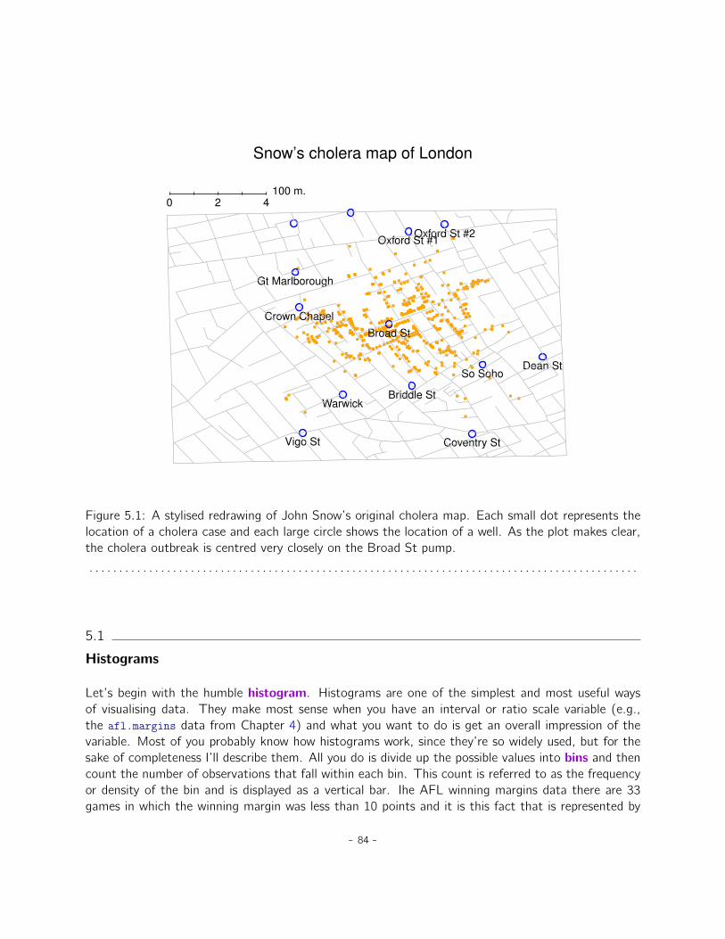
Snow’s cholera map of London

Oxford St #1Oxford St #2

Gt Marlborough

Crown Chapel

Broad St

WarwickBriddle St

So SohoDean St

Coventry StVigo St

0 2 4100 m.

Figure 5.1: A stylised redrawing of John Snow’s original cholera map. Each small dot represents thelocation of a cholera case and each large circle shows the location of a well. As the plot makes clear,the cholera outbreak is centred very closely on the Broad St pump.

. . . . . . . . . . . . . . . . . . . . . . . . . . . . . . . . . . . . . . . . . . . . . . . . . . . . . . . . . . . . . . . . . . . . . . . . . . . . . . . . . . . . . . . . . . . .

5.1

Histograms

Let’s begin with the humble histogram. Histograms are one of the simplest and most useful waysof visualising data. They make most sense when you have an interval or ratio scale variable (e.g.,the afl.margins data from Chapter 4) and what you want to do is get an overall impression of thevariable. Most of you probably know how histograms work, since they’re so widely used, but for thesake of completeness I’ll describe them. All you do is divide up the possible values into bins and thencount the number of observations that fall within each bin. This count is referred to as the frequencyor density of the bin and is displayed as a vertical bar. Ihe AFL winning margins data there are 33games in which the winning margin was less than 10 points and it is this fact that is represented by

- 84 -

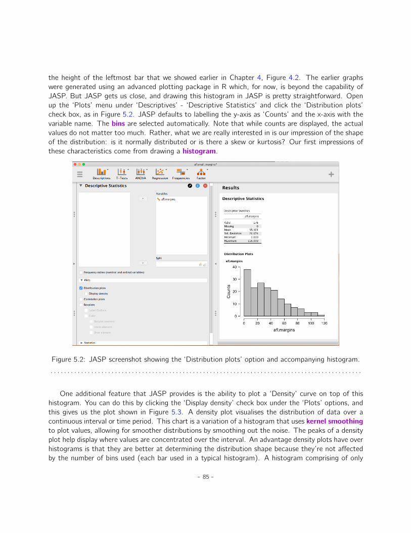
the height of the leftmost bar that we showed earlier in Chapter 4, Figure 4.2. The earlier graphswere generated using an advanced plotting package in R which, for now, is beyond the capability ofJASP. But JASP gets us close, and drawing this histogram in JASP is pretty straightforward. Openup the ‘Plots’ menu under ‘Descriptives’ - ‘Descriptive Statistics’ and click the ‘Distribution plots’check box, as in Figure 5.2. JASP defaults to labelling the y-axis as ‘Counts’ and the x-axis with thevariable name. The bins are selected automatically. Note that while counts are displayed, the actualvalues do not matter too much. Rather, what we are really interested in is our impression of the shapeof the distribution: is it normally distributed or is there a skew or kurtosis? Our first impressions ofthese characteristics come from drawing a histogram.

Figure 5.2: JASP screenshot showing the ‘Distribution plots’ option and accompanying histogram.

. . . . . . . . . . . . . . . . . . . . . . . . . . . . . . . . . . . . . . . . . . . . . . . . . . . . . . . . . . . . . . . . . . . . . . . . . . . . . . . . . . . . . . . . . . . .

One additional feature that JASP provides is the ability to plot a ‘Density’ curve on top of thishistogram. You can do this by clicking the ‘Display density’ check box under the ‘Plots’ options, andthis gives us the plot shown in Figure 5.3. A density plot visualises the distribution of data over acontinuous interval or time period. This chart is a variation of a histogram that uses kernel smoothingto plot values, allowing for smoother distributions by smoothing out the noise. The peaks of a densityplot help display where values are concentrated over the interval. An advantage density plots have overhistograms is that they are better at determining the distribution shape because they’re not affectedby the number of bins used (each bar used in a typical histogram). A histogram comprising of only

- 85 -

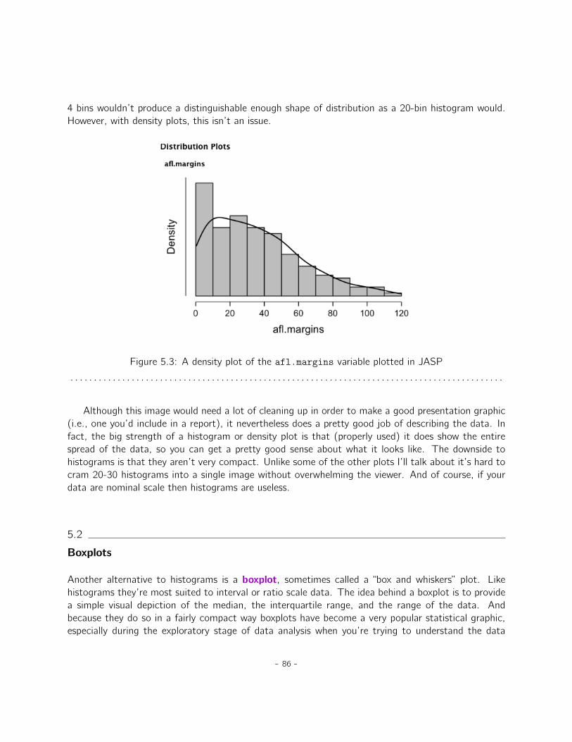
4 bins wouldn’t produce a distinguishable enough shape of distribution as a 20-bin histogram would.However, with density plots, this isn’t an issue.

Figure 5.3: A density plot of the afl.margins variable plotted in JASP

. . . . . . . . . . . . . . . . . . . . . . . . . . . . . . . . . . . . . . . . . . . . . . . . . . . . . . . . . . . . . . . . . . . . . . . . . . . . . . . . . . . . . . . . . . . .

Although this image would need a lot of cleaning up in order to make a good presentation graphic(i.e., one you’d include in a report), it nevertheless does a pretty good job of describing the data. Infact, the big strength of a histogram or density plot is that (properly used) it does show the entirespread of the data, so you can get a pretty good sense about what it looks like. The downside tohistograms is that they aren’t very compact. Unlike some of the other plots I’ll talk about it’s hard tocram 20-30 histograms into a single image without overwhelming the viewer. And of course, if yourdata are nominal scale then histograms are useless.

5.2

Boxplots

Another alternative to histograms is a boxplot, sometimes called a “box and whiskers” plot. Likehistograms they’re most suited to interval or ratio scale data. The idea behind a boxplot is to providea simple visual depiction of the median, the interquartile range, and the range of the data. Andbecause they do so in a fairly compact way boxplots have become a very popular statistical graphic,especially during the exploratory stage of data analysis when you’re trying to understand the data

- 86 -

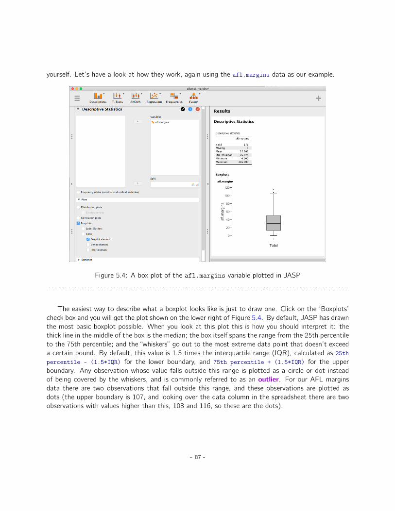
yourself. Let’s have a look at how they work, again using the afl.margins data as our example.

Figure 5.4: A box plot of the afl.margins variable plotted in JASP

. . . . . . . . . . . . . . . . . . . . . . . . . . . . . . . . . . . . . . . . . . . . . . . . . . . . . . . . . . . . . . . . . . . . . . . . . . . . . . . . . . . . . . . . . . . .

The easiest way to describe what a boxplot looks like is just to draw one. Click on the ‘Boxplots’check box and you will get the plot shown on the lower right of Figure 5.4. By default, JASP has drawnthe most basic boxplot possible. When you look at this plot this is how you should interpret it: thethick line in the middle of the box is the median; the box itself spans the range from the 25th percentileto the 75th percentile; and the “whiskers” go out to the most extreme data point that doesn’t exceeda certain bound. By default, this value is 1.5 times the interquartile range (IQR), calculated as 25thpercentile - (1.5*IQR) for the lower boundary, and 75th percentile + (1.5*IQR) for the upperboundary. Any observation whose value falls outside this range is plotted as a circle or dot insteadof being covered by the whiskers, and is commonly referred to as an outlier. For our AFL marginsdata there are two observations that fall outside this range, and these observations are plotted asdots (the upper boundary is 107, and looking over the data column in the spreadsheet there are twoobservations with values higher than this, 108 and 116, so these are the dots).

- 87 -

Figure 5.5: A violin plot of the afl.margins variable plotted in JASP, also showing a box plot anddata points

. . . . . . . . . . . . . . . . . . . . . . . . . . . . . . . . . . . . . . . . . . . . . . . . . . . . . . . . . . . . . . . . . . . . . . . . . . . . . . . . . . . . . . . . . . . .

5.2.1 Violin plots

A variation to the traditional box plot is the violin plot. Violin plots are similar to box plots exceptthat they also show the kernel probability density of the data at different values. Typically, violin plotswill include a marker for the median of the data and a box indicating the interquartile range, as instandard box plots. In JASP you can achieve this sort of functionality by checking both the ‘Violinelement’ and the ’Boxplot element’ check boxes. See Figure 5.5, which also has the data plotted(select the ‘Jitter element’ check box to show the actual data points on the plot).

5.2.2 Drawing multiple boxplots

One last thing. What if you want to draw multiple boxplots at once? Suppose, for instance,I wanted separate boxplots showing the AFL margins not just for 2010 but for every year between1987 and 2010. To do that the first thing we’ll have to do is find the data. These are stored in theaflsmall2.csv file. So let’s load it into JASP and see what is in it. You will see that it is a prettybig data set. It contains 4296 games and the variables that we’re interested in. What we want to dois have JASP draw boxplots for the margin variable, but plotted separately for each year. The way todo this is to first change year to a nominal variable, then year across into the ‘Split’ box.

The result is shown in Figure 5.6. This version of the box plot, split by year, gives a sense of why

- 88 -

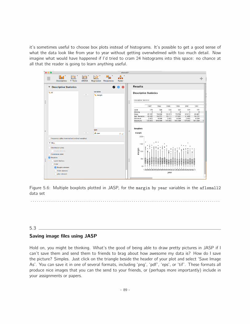
it’s sometimes useful to choose box plots instead of histograms. It’s possible to get a good sense ofwhat the data look like from year to year without getting overwhelmed with too much detail. Nowimagine what would have happened if I’d tried to cram 24 histograms into this space: no chance atall that the reader is going to learn anything useful.

Figure 5.6: Multiple boxplots plotted in JASP, for the margin by year variables in the aflsmall2data set

. . . . . . . . . . . . . . . . . . . . . . . . . . . . . . . . . . . . . . . . . . . . . . . . . . . . . . . . . . . . . . . . . . . . . . . . . . . . . . . . . . . . . . . . . . . .

5.3

Saving image files using JASP

Hold on, you might be thinking. What’s the good of being able to draw pretty pictures in JASP if Ican’t save them and send them to friends to brag about how awesome my data is? How do I savethe picture? Simples. Just click on the triangle beside the header of your plot and select ‘Save ImageAs’. You can save it in one of several formats, including ‘png’, ‘pdf’, ‘eps’, or ‘tif’. These formats allproduce nice images that you can the send to your friends, or (perhaps more importantly) include inyour assignments or papers.

- 89 -

5.4

Summary

Perhaps I’m a simple minded person, but I love pictures. Every time I write a new scientific paper oneof the first things I do is sit down and think about what the pictures will be. In my head an article isreally just a sequence of pictures linked together by a story. All the rest of it is just window dressing.What I’m really trying to say here is that the human visual system is a very powerful data analysistool. Give it the right kind of information and it will supply a human reader with a massive amount ofknowledge very quickly. Not for nothing do we have the saying “a picture is worth a thousand words”.With that in mind, I think that this is one of the most important chapters in the book. The topicscovered were:

• Common plots. Much of the chapter was focused on some of the standard graphs that statis-ticians like to produce: histograms (Section 5.1) and boxplots (Section 5.2)

• Saving image files. Importantly, we also covered how to export your pictures (Section 5.3)

One final thing to point out. While JASP produces some really neat default graphics, editingthe plots is currently not possible. For more advanced graphics and plotting capability the packagesavailable in R are much more powerful. One of the most popular graphics systems is provided by theggplot2 package (see http://ggplot2.org/), which is loosely based on “The grammar of graphics”(Wilkinson, Wills, Rope, Norton, and Dubbs 2006). It’s not for novices. You need to have a prettygood grasp of R before you can start using it, and even then it takes a while to really get the hangof it. But when you’re ready it’s worth taking the time to teach yourself, because it’s a much morepowerful and cleaner system.

- 90 -

http://ggplot2.org/

Part III.

Statistical theory

- 91 -

Prelude to Part IV

Part IV of the book is by far the most theoretical, focusing as it does on the theory of statisticalinference. Over the next three chapters my goal is to give you an introduction to probability theory(Chapter 6), sampling and estimation (Chapter 7) and statistical hypothesis testing (Chapter 8).Before we get started though, I want to say something about the big picture. Statistical inference isprimarily about learning from data. The goal is no longer merely to describe our data but to use thedata to draw conclusions about the world. To motivate the discussion I want to spend a bit of timetalking about a philosophical puzzle known as the riddle of induction, because it speaks to an issue thatwill pop up over and over again throughout the book: statistical inference relies on assumptions. Thissounds like a bad thing. In everyday life people say things like “you should never make assumptions”,and psychology classes often talk about assumptions and biases as bad things that we should try toavoid. From bitter personal experience I have learned never to say such things around philosophers!

On the limits of logical reasoning

The whole art of war consists in getting at what is on the other side of the hill, or, inother words, in learning what we do not know from what we do.

– Arthur Wellesley, 1st Duke of Wellington

I am told that quote above came about as a consequence of a carriage ride across the countryside.2

He and his companion, J. W. Croker, were playing a guessing game, each trying to predict what wouldbe on the other side of each hill. In every case it turned out that Wellesley was right and Croker waswrong. Many years later when Wellesley was asked about the game he explained that “the whole artof war consists in getting at what is on the other side of the hill”. Indeed, war is not special in thisrespect. All of life is a guessing game of one form or another, and getting by on a day to day basisrequires us to make good guesses. So let’s play a guessing game of our own.

Suppose you and I are observing the Wellesley-Croker competition and after every three hills youand I have to predict who will win the next one, Wellesley or Croker. Let’s say that W refers to aWellesley victory and C refers to a Croker victory. After three hills, our data set looks like this:

WWW

Our conversation goes like this:2Source: http://www.bartleby.com/344/400.html.

- 93 -

http://www.bartleby.com/344/400.html

you: Three in a row doesn’t mean much. I suppose Wellesley might be better at thisthan Croker, but it might just be luck. Still, I’m a bit of a gambler. I’ll bet onWellesley.

me: I agree that three in a row isn’t informative and I see no reason to preferWellesley’s guesses over Croker’s. I can’t justify betting at this stage. Sorry.No bet for me.

Your gamble paid off: three more hills go by and Wellesley wins all three. Going into the nextround of our game the score is 1-0 in favour of you and our data set looks like this:

WWW WWW

I’ve organised the data into blocks of three so that you can see which batch corresponds to theobservations that we had available at each step in our little side game. After seeing this new batch,our conversation continues:

you: Six wins in a row for Duke Wellesley. This is starting to feel a bit suspicious.I’m still not certain, but I reckon that he’s going to win the next one too.

me: I guess I don’t see that. Sure, I agree that Wellesley has won six in a row, but Idon’t see any logical reason why that means he’ll win the seventh one. No bet.

you: Do you really think so? Fair enough, but my bet worked out last time and I’mokay with my choice.

For a second time you were right, and for a second time I was wrong. Wellesley wins the nextthree hills, extending his winning record against Croker to 9-0. The data set available to us is nowthis:

WWW WWW WWW

And our conversation goes like this:

you: Okay, this is pretty obvious. Wellesley is way better at this game. We bothagree he’s going to win the next hill, right?

me: Is there really any logical evidence for that? Before we started this game, therewere lots of possibilities for the first 10 outcomes, and I had no idea which oneto expect. WWW WWW WWW W was one possibility, but so was WCC CWC WWC C andWWW WWW WWW C or even CCC CCC CCC C. Because I had no idea what wouldhappen so I’d have said they were all equally likely. I assume you would havetoo, right? I mean, that’s what it means to say you have “no idea”, isn’t it?

you: I suppose so.

- 94 -

me: Well then, the observations we’ve made logically rule out all possibilities excepttwo: WWW WWW WWW C or WWW WWW WWW W. Both of these are perfectly consistentwith the evidence we’ve encountered so far, aren’t they?

you: Yes, of course they are. Where are you going with this?

me: So what’s changed then? At the start of our game, you’d have agreed with methat these are equally plausible and none of the evidence that we’ve encounteredhas discriminated between these two possibilities. Therefore, both of thesepossibilities remain equally plausible and I see no logical reason to prefer oneover the other. So yes, while I agree with you that Wellesley’s run of 9 wins ina row is remarkable, I can’t think of a good reason to think he’ll win the 10thhill. No bet.

you: I see your point, but I’m still willing to chance it. I’m betting on Wellesley.

Wellesley’s winning streak continues for the next three hills. The score in the Wellesley-Croker gameis now 12-0, and the score in our game is now 3-0. As we approach the fourth round of our game,our data set is this:

WWW WWW WWW WWW

and the conversation continues:

you: Oh yeah! Three more wins for Wellesley and another victory for me. Admit it, Iwas right about him! I guess we’re both betting on Wellesley this time around,right?

me: I don’t know what to think. I feel like we’re in the same situation we werein last round, and nothing much has changed. There are only two legitimatepossibilities for a sequence of 13 hills that haven’t already been ruled out, WWWWWW WWW WWW C and WWW WWW WWW WWW W. It’s just like I said last time. If allpossible outcomes were equally sensible before the game started, shouldn’t thesetwo be equally sensible now given that our observations don’t rule out eitherone? I agree that it feels like Wellesley is on an amazing winning streak, butwhere’s the logical evidence that the streak will continue?

you: I think you’re being unreasonable. Why not take a look at our scorecard, if youneed evidence? You’re the expert on statistics and you’ve been using this fancylogical analysis, but the fact is you’re losing. I’m just relying on common senseand I’m winning. Maybe you should switch strategies.

me: Hmm, that is a good point and I don’t want to lose the game, but I’m afraid Idon’t see any logical evidence that your strategy is better than mine. It seemsto me that if there were someone else watching our game, what they’d haveobserved is a run of three wins to you. Their data would look like this: YYY.

- 95 -

Logically, I don’t see that this is any different to our first round of watchingWellesley and Croker. Three wins to you doesn’t seem like a lot of evidence,and I see no reason to think that your strategy is working out any better thanmine. If I didn’t think that WWW was good evidence then for Wellesley beingbetter than Croker at their game, surely I have no reason now to think that YYYis good evidence that you’re better at ours?

you: Okay, now I think you’re being a jerk.

me: I don’t see the logical evidence for that.

Learning without making assumptions is a myth

There are lots of different ways in which we could dissect this dialogue, but since this is a statisticsbook pitched at psychologists and not an introduction to the philosophy and psychology of reasoning,I’ll keep it brief. What I’ve described above is sometimes referred to as the riddle of induction. Itseems entirely reasonable to think that a 12-0 winning record by Wellesley is pretty strong evidencethat he will win the 13th game, but it is not easy to provide a proper logical justification for this belief.On the contrary, despite the obviousness of the answer, it’s not actually possible to justify betting onWellesley without relying on some assumption that you don’t have any logical justification for.

The riddle of induction is most associated with the philosophical work of David Hume and morerecently Nelson Goodman, but you can find examples of the problem popping up in fields as diverse asliterature (Lewis Carroll) and machine learning (the “no free lunch” theorem). There really is somethingweird about trying to “learn what we do not know from what we do know”. The critical point is thatassumptions and biases are unavoidable if you want to learn anything about the world. There is noescape from this, and it is just as true for statistical inference as it is for human reasoning. In thedialogue I was taking aim at your perfectly sensible inferences as a human being, but the common sensereasoning that you relied on is no different to what a statistician would have done. Your “commonsense” half of the dialog relied on an implicit assumption that there exists some difference in skillbetween Wellesley and Croker, and what you were doing was trying to work out what that differencein skill level would be. My “logical analysis” rejects that assumption entirely. All I was willing to acceptis that there are sequences of wins and losses and that I did not know which sequences would beobserved. Throughout the dialogue I kept insisting that all logically possible data sets were equallyplausible at the start of the Wellesely-Croker game, and the only way in which I ever revised my beliefswas to eliminate those possibilities that were factually inconsistent with the observations.

That sounds perfectly sensible on its own terms. In fact, it even sounds like the hallmark of gooddeductive reasoning. Like Sherlock Holmes, my approach was to rule out that which is impossible inthe hope that what would be left is the truth. Yet as we saw, ruling out the impossible never led me tomake a prediction. On its own terms everything I said in my half of the dialogue was entirely correct.An inability to make any predictions is the logical consequence of making “no assumptions”. In theend I lost our game because you did make some assumptions and those assumptions turned out to

- 96 -

be right. Skill is a real thing, and because you believed in the existence of skill you were able to learnthat Wellesley had more of it than Croker. Had you relied on a less sensible assumption to drive yourlearning you might not have won the game.

Ultimately there are two things you should take away from this. First, as I’ve said, you cannot avoidmaking assumptions if you want to learn anything from your data. But second, once you realise thatassumptions are necessary it becomes important to make sure you make the right ones! A data analysisthat relies on few assumptions is not necessarily better than one that makes many assumptions, it alldepends on whether those assumptions are good ones for your data. As we go through the rest ofthis book I’ll often point out the assumptions that underpin a particular statistical technique, and howyou can check whether those assumptions are sensible.

- 97 -

- 98 -

6. Introduction to probability

[God] has afforded us only the twilight . . . of Probability.

– John Locke

Up to this point in the book we’ve discussed some of the key ideas in experimental design, andwe’ve talked a little about how you can summarise a data set. To a lot of people this is all there is tostatistics: collecting all the numbers, calculating averages, drawing pictures, and putting them all in areport somewhere. Kind of like stamp collecting but with numbers. However, statistics covers muchmore than that. In fact, descriptive statistics is one of the smallest parts of statistics and one of theleast powerful. The bigger and more useful part of statistics is that it provides information that letsyou make inferences about data.

Once you start thinking about statistics in these terms, that statistics is there to help us drawinferences from data, you start seeing examples of it everywhere. For instance, here’s a tiny extractfrom a newspaper article in the Sydney Morning Herald (30 Oct 2010):

“I have a tough job,” the Premier said in response to a poll which found her government is now themost unpopular Labor administration in polling history, with a primary vote of just 23 per cent.

This kind of remark is entirely unremarkable in the papers or in everyday life, but let’s have a thinkabout what it entails. A polling company has conducted a survey, usually a pretty big one becausethey can afford it. I’m too lazy to track down the original survey so let’s just imagine that theycalled 1000 New South Wales (NSW) voters at random, and 230 (23%) of those claimed that theyintended to vote for the Australian Labor Party (ALP). For the 2010 Federal election the AustralianElectoral Commission reported 4,610,795 enrolled voters in NSW, so the opinions of the remaining4,609,795 voters (about 99.98% of voters) remain unknown to us. Even assuming that no-one lied tothe polling company the only thing we can say with 100% confidence is that the true ALP primary voteis somewhere between 230/4610795 (about 0.005%) and 4610025/4610795 (about 99.83%). So,on what basis is it legitimate for the polling company, the newspaper, and the readership to concludethat the ALP primary vote is only about 23%?

The answer to the question is pretty obvious. If I call 1000 people at random, and 230 of themsay they intend to vote for the ALP, then it seems very unlikely that these are the only 230 people

- 99 -

out of the entire voting public who actually intend to vote ALP. In other words, we assume that thedata collected by the polling company is pretty representative of the population at large. But howrepresentative? Would we be surprised to discover that the true ALP primary vote is actually 24%?29%? 37%? At this point everyday intuition starts to break down a bit. No-one would be surprised by24%, and everybody would be surprised by 37%, but it’s a bit hard to say whether 29% is plausible.We need some more powerful tools than just looking at the numbers and guessing.

Inferential statistics provides the tools that we need to answer these sorts of questions, and sincethese kinds of questions lie at the heart of the scientific enterprise, they take up the lions share of everyintroductory course on statistics and research methods. However, the theory of statistical inferenceis built on top of probability theory. And it is to probability theory that we must now turn. Thisdiscussion of probability theory is basically background detail. There’s not a lot of statistics per se inthis chapter, and you don’t need to understand this material in as much depth as the other chaptersin this part of the book. Nevertheless, because probability theory does underpin so much of statistics,it’s worth covering some of the basics.

6.1

How are probability and statistics different?

Before we start talking about probability theory, it’s helpful to spend a moment thinking about therelationship between probability and statistics. The two disciplines are closely related but they’re notidentical. Probability theory is “the doctrine of chances”. It’s a branch of mathematics that tells youhow often different kinds of events will happen. For example, all of these questions are things you cananswer using probability theory:

• What are the chances of a fair coin coming up heads 10 times in a row?

• If I roll a six sided dice twice, how likely is it that I’ll roll two sixes?

• How likely is it that five cards drawn from a perfectly shuffled deck will all be hearts?

• What are the chances that I’ll win the lottery?

Notice that all of these questions have something in common. In each case the “truth of the world”is known and my question relates to the “what kind of events” will happen. In the first question I knowthat the coin is fair so there’s a 50% chance that any individual coin flip will come up heads. In thesecond question I know that the chance of rolling a 6 on a single die is 1 in 6. In the third questionI know that the deck is shuffled properly. And in the fourth question I know that the lottery followsspecific rules. You get the idea. The critical point is that probabilistic questions start with a knownmodel of the world, and we use that model to do some calculations. The underlying model can bequite simple. For instance, in the coin flipping example we can write down the model like this:

P pheadsq “ 0.5

- 100 -

which you can read as “the probability of heads is 0.5”. As we’ll see later, in the same way thatpercentages are numbers that range from 0% to 100%, probabilities are just numbers that range from0 to 1. When using this probability model to answer the first question I don’t actually know exactlywhat’s going to happen. Maybe I’ll get 10 heads, like the question says. But maybe I’ll get threeheads. That’s the key thing. In probability theory the model is known but the data are not.

So that’s probability. What about statistics? Statistical questions work the other way around. Instatistics we do not know the truth about the world. All we have is the data and it is from the datathat we want to learn the truth about the world. Statistical questions tend to look more like these:

• If my friend flips a coin 10 times and gets 10 heads are they playing a trick on me?• If five cards off the top of the deck are all hearts how likely is it that the deck was shuffled?• If the lottery commissioner’s spouse wins the lottery how likely is it that the lottery was rigged?

This time around the only thing we have are data. What I know is that I saw my friend flip thecoin 10 times and it came up heads every time. And what I want to infer is whether or not I shouldconclude that what I just saw was actually a fair coin being flipped 10 times in a row, or whether Ishould suspect that my friend is playing a trick on me. The data I have look like this:

H H H H H H H H H H H

and what I’m trying to do is work out which “model of the world” I should put my trust in. If thecoin is fair then the model I should adopt is one that says that the probability of heads is 0.5, thatis P pheadsq “ 0.5. If the coin is not fair then I should conclude that the probability of heads is not0.5, which we would write as P pheadsq ‰ 0.5. In other words, the statistical inference problem is tofigure out which of these probability models is right. Clearly, the statistical question isn’t the sameas the probability question, but they’re deeply connected to one another. Because of this, a goodintroduction to statistical theory will start with a discussion of what probability is and how it works.

6.2

What does probability mean?

Let’s start with the first of these questions. What is “probability”? It might seem surprising to youbut while statisticians and mathematicians (mostly) agree on what the rules of probability are, there’smuch less of a consensus on what the word really means. It seems weird because we’re all verycomfortable using words like “chance”, “likely”, “possible” and “probable”, and it doesn’t seem like itshould be a very difficult question to answer. But if you’ve ever had that experience in real life youmight walk away from the conversation feeling like you didn’t quite get it right, and that (like manyeveryday concepts) it turns out that you don’t really know what it’s all about.

So I’ll have a go at it. Let’s suppose I want to bet on a soccer game between two teams of robots,Arduino Arsenal and C Milan. After thinking about it, I decide that there is an 80% probability ofArduino Arsenal winning. What do I mean by that? Here are three possibilities:

- 101 -

• They’re robot teams so I can make them play over and over again, and if I did that ArduinoArsenal would win 8 out of every 10 games on average.

• For any given game, I would agree that betting on this game is only “fair” if a $1 bet on C Milangives a $5 payoff (i.e. I get my $1 back plus a $4 reward for being correct), as would a $4 beton Arduino Arsenal (i.e., my $4 bet plus a $1 reward).

• My subjective “belief” or “confidence” in an Arduino Arsenal victory is four times as strong asmy belief in a C Milan victory.

Each of these seems sensible. However, they’re not identical and not every statistician would endorseall of them. The reason is that there are different statistical ideologies (yes, really!) and depending onwhich one you subscribe to, you might say that some of those statements are meaningless or irrelevant.In this section I give a brief introduction the two main approaches that exist in the literature. Theseare by no means the only approaches, but they’re the two big ones.

6.2.1 The frequentist view

The first of the two major approaches to probability, and the more dominant one in statistics, isreferred to as the frequentist view and it defines probability as a long-run frequency. Suppose wewere to try flipping a fair coin over and over again. By definition this is a coin that has P pHq “ 0.5.What might we observe? One possibility is that the first 20 flips might look like this:

T,H,H,H,H,T,T,H,H,H,H,T,H,H,T,T,T,T,T,H

In this case 11 of these 20 coin flips (55%) came up heads. Now suppose that I’d been keeping arunning tally of the number of heads (which I’ll call NH) that I’ve seen, across the first N flips, andcalculate the proportion of heads NH{N every time. Here’s what I’d get (I did literally flip coins toproduce this!):

number of flips 1 2 3 4 5 6 7 8 9 10number of heads 0 1 2 3 4 4 4 5 6 7proportion .00 .50 .67 .75 .80 .67 .57 .63 .67 .70

number of flips 11 12 13 14 15 16 17 18 19 20number of heads 8 8 9 10 10 10 10 10 10 11proportion .73 .67 .69 .71 .67 .63 .59 .56 .53 .55

Notice that at the start of the sequence the proportion of heads fluctuates wildly, starting at .00and rising as high as .80. Later on, one gets the impression that it dampens out a bit, with moreand more of the values actually being pretty close to the “right” answer of .50. This is the frequentistdefinition of probability in a nutshell. Flip a fair coin over and over again, and as N grows large

- 102 -

(approaches infinity, denoted N Ñ8) the proportion of heads will converge to 50%. There are somesubtle technicalities that the mathematicians care about, but qualitatively speaking that’s how thefrequentists define probability. Unfortunately, I don’t have an infinite number of coins or the infinitepatience required to flip a coin an infinite number of times. However, I do have a computer andcomputers excel at mindless repetitive tasks. So I asked my computer to simulate flipping a coin 1000times and then drew a picture of what happens to the proportion NH{N as N increases. Actually, Idid it four times just to make sure it wasn’t a fluke. The results are shown in Figure 6.1. As you cansee, the proportion of observed heads eventually stops fluctuating and settles down. When it does,the number at which it finally settles is the true probability of heads.

The frequentist definition of probability has some desirable characteristics. First, it is objective.The probability of an event is necessarily grounded in the world. The only way that probabilitystatements can make sense is if they refer to (a sequence of) events that occur in the physicaluniverse.1 Secondly, it is unambiguous. Any two people watching the same sequence of events unfold,trying to calculate the probability of an event, must inevitably come up with the same answer.

However, it also has undesirable characteristics. First, infinite sequences don’t exist in the physicalworld. Suppose you picked up a coin from your pocket and started to flip it. Every time it lands itimpacts on the ground. Each impact wears the coin down a bit. Eventually the coin will be destroyed.So, one might ask whether it really makes sense to pretend that an “infinite” sequence of coin flips iseven a meaningful concept, or an objective one. We can’t say that an “infinite sequence” of eventsis a real thing in the physical universe, because the physical universe doesn’t allow infinite anything.More seriously, the frequentist definition has a narrow scope. There are lots of things out there thathuman beings are happy to assign probability to in everyday language, but cannot (even in theory) bemapped onto a hypothetical sequence of events. For instance, if a meteorologist comes on TV andsays “the probability of rain in Adelaide on 2 November 2048 is 60%” we humans are happy to acceptthis. But it’s not clear how to define this in frequentist terms. There’s only one city of Adelaide,and only one 2 November 2048. There’s no infinite sequence of events here, just a one-off thing.Frequentist probability genuinely forbids us from making probability statements about a single event.From the frequentist perspective it will either rain tomorrow or it will not. There is no “probability”that attaches to a single non-repeatable event. Now, it should be said that there are some very clevertricks that frequentists can use to get around this. One possibility is that what the meteorologistmeans is something like “There is a category of days for which I predict a 60% chance of rain, andif we look only across those days for which I make this prediction, then on 60% of those days it willactually rain”. It’s very weird and counterintuitive to think of it this way, but you do see frequentistsdo this sometimes. And it will come up later in this book (see Section 7.5).

1This doesn’t mean that frequentists can’t make hypothetical statements, of course. It’s just that if you want to makea statement about probability then it must be possible to redescribe that statement in terms of a sequence of potentiallyobservable events, together with the relative frequencies of different outcomes that appear within that sequence.

- 103 -

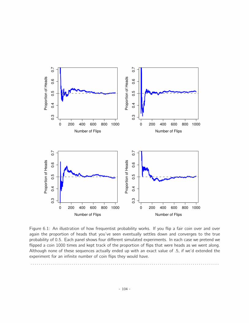
0 200 400 600 800 1000

0.3

0.4

0.5

0.6

0.7

Number of Flips

Pro

po

rtio

n o

f H

ea

ds

0 200 400 600 800 1000

0.3

0.4

0.5

0.6

0.7

Number of Flips

Pro

po

rtio

n o

f H

ea

ds

0 200 400 600 800 1000

0.3

0.4

0.5

0.6

0.7

Number of Flips

Pro

po

rtio

n o

f H

ea

ds

0 200 400 600 800 1000

0.3

0.4

0.5

0.6

0.7

Number of Flips

Pro

po

rtio

n o

f H

ea

ds

Figure 6.1: An illustration of how frequentist probability works. If you flip a fair coin over and overagain the proportion of heads that you’ve seen eventually settles down and converges to the trueprobability of 0.5. Each panel shows four different simulated experiments. In each case we pretend weflipped a coin 1000 times and kept track of the proportion of flips that were heads as we went along.Although none of these sequences actually ended up with an exact value of .5, if we’d extended theexperiment for an infinite number of coin flips they would have.

. . . . . . . . . . . . . . . . . . . . . . . . . . . . . . . . . . . . . . . . . . . . . . . . . . . . . . . . . . . . . . . . . . . . . . . . . . . . . . . . . . . . . . . . . . . .

- 104 -

6.2.2 The Bayesian view

The Bayesian view of probability is often called the subjectivist view, and although it has beena minority view among statisticians it has been steadily gaining traction for the last several decades.There are many flavours of Bayesianism, making it hard to say exactly what “the” Bayesian view is.The most common way of thinking about subjective probability is to define the probability of an eventas the degree of belief that an intelligent and rational agent assigns to that truth of that event. Fromthat perspective, probabilities don’t exist in the world but rather in the thoughts and assumptions ofpeople and other intelligent beings.

However, in order for this approach to work we need some way of operationalising “degree of belief”.One way that you can do this is to formalise it in terms of “rational gambling”, though there are manyother ways. Suppose that I believe that there’s a 60% probability of rain tomorrow. If someone offersme a bet that if it rains tomorrow then I win $5, but if it doesn’t rain I lose $5. Clearly, from myperspective, this is a pretty good bet. On the other hand, if I think that the probability of rain is only40% then it’s a bad bet to take. So we can operationalise the notion of a “subjective probability” interms of what bets I’m willing to accept.

What are the advantages and disadvantages to the Bayesian approach? The main advantage isthat it allows you to assign probabilities to any event you want to. You don’t need to be limited tothose events that are repeatable. The main disadvantage (to many people) is that we can’t be purelyobjective. Specifying a probability requires us to specify an entity that has the relevant degree ofbelief. This entity might be a human, an alien, a robot, or even a statistician. But there has to bean intelligent agent out there that believes in things. To many people this is uncomfortable, it seemsto make probability arbitrary. Whilst the Bayesian approach requires that the agent in question berational (i.e., obey the rules of probability), it does allow everyone to have their own beliefs. I canbelieve the coin is fair and you don’t have to, even though we’re both rational. The frequentist viewdoesn’t allow any two observers to attribute different probabilities to the same event. When thathappens then at least one of them must be wrong. The Bayesian view does not prevent this fromoccurring. Two observers with different background knowledge can legitimately hold different beliefsabout the same event. In short, where the frequentist view is sometimes considered to be too narrow(forbids lots of things that that we want to assign probabilities to), the Bayesian view is sometimesthought to be too broad (allows too many differences between observers).

6.2.3 What’s the difference? And who is right?

Now that you’ve seen each of these two views independently it’s useful to make sure you cancompare the two. Go back to the hypothetical robot soccer game at the start of the section. Whatdo you think a frequentist and a Bayesian would say about these three statements? Which statementwould a frequentist say is the correct definition of probability? Which one would a Bayesian opt for?Would some of these statements be meaningless to a frequentist or a Bayesian? If you’ve understoodthe two perspectives you should have some sense of how to answer those questions.

Okay, assuming you understand the difference then you might be wondering which of them is

- 105 -

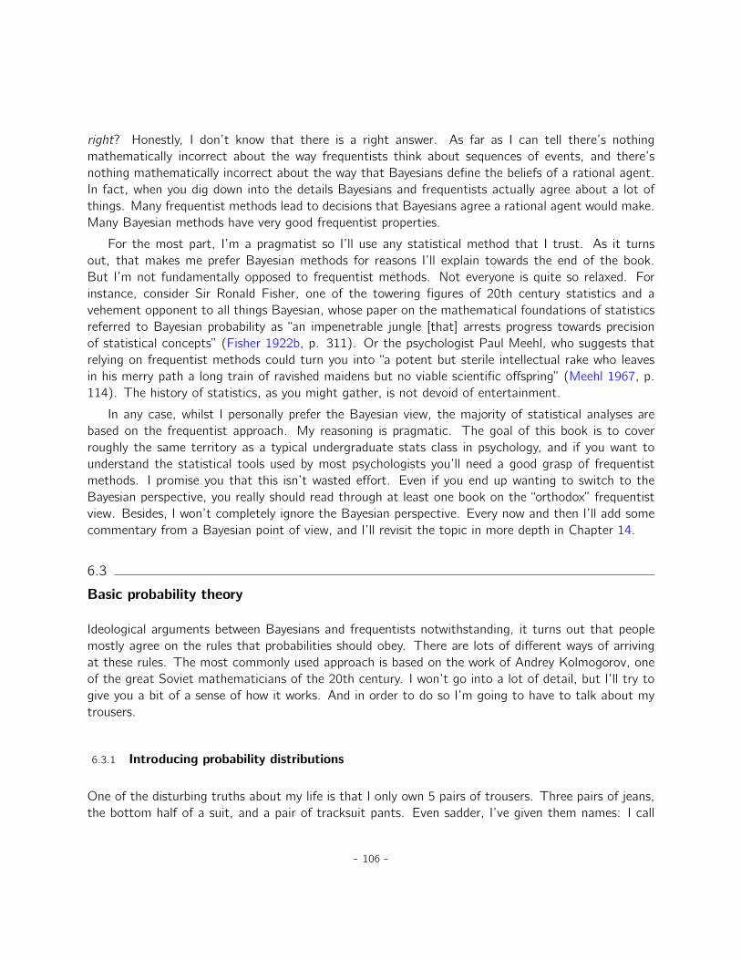
right? Honestly, I don’t know that there is a right answer. As far as I can tell there’s nothingmathematically incorrect about the way frequentists think about sequences of events, and there’snothing mathematically incorrect about the way that Bayesians define the beliefs of a rational agent.In fact, when you dig down into the details Bayesians and frequentists actually agree about a lot ofthings. Many frequentist methods lead to decisions that Bayesians agree a rational agent would make.Many Bayesian methods have very good frequentist properties.

For the most part, I’m a pragmatist so I’ll use any statistical method that I trust. As it turnsout, that makes me prefer Bayesian methods for reasons I’ll explain towards the end of the book.But I’m not fundamentally opposed to frequentist methods. Not everyone is quite so relaxed. Forinstance, consider Sir Ronald Fisher, one of the towering figures of 20th century statistics and avehement opponent to all things Bayesian, whose paper on the mathematical foundations of statisticsreferred to Bayesian probability as “an impenetrable jungle [that] arrests progress towards precisionof statistical concepts” (Fisher 1922b, p. 311). Or the psychologist Paul Meehl, who suggests thatrelying on frequentist methods could turn you into “a potent but sterile intellectual rake who leavesin his merry path a long train of ravished maidens but no viable scientific offspring” (Meehl 1967, p.114). The history of statistics, as you might gather, is not devoid of entertainment.

In any case, whilst I personally prefer the Bayesian view, the majority of statistical analyses arebased on the frequentist approach. My reasoning is pragmatic. The goal of this book is to coverroughly the same territory as a typical undergraduate stats class in psychology, and if you want tounderstand the statistical tools used by most psychologists you’ll need a good grasp of frequentistmethods. I promise you that this isn’t wasted effort. Even if you end up wanting to switch to theBayesian perspective, you really should read through at least one book on the “orthodox” frequentistview. Besides, I won’t completely ignore the Bayesian perspective. Every now and then I’ll add somecommentary from a Bayesian point of view, and I’ll revisit the topic in more depth in Chapter 14.

6.3

Basic probability theory

Ideological arguments between Bayesians and frequentists notwithstanding, it turns out that peoplemostly agree on the rules that probabilities should obey. There are lots of different ways of arrivingat these rules. The most commonly used approach is based on the work of Andrey Kolmogorov, oneof the great Soviet mathematicians of the 20th century. I won’t go into a lot of detail, but I’ll try togive you a bit of a sense of how it works. And in order to do so I’m going to have to talk about mytrousers.

6.3.1 Introducing probability distributions

One of the disturbing truths about my life is that I only own 5 pairs of trousers. Three pairs of jeans,the bottom half of a suit, and a pair of tracksuit pants. Even sadder, I’ve given them names: I call

- 106 -

them X1, X2, X3, X4 and X5. I really have, that’s why they call me Mister Imaginative. Now, onany given day, I pick out exactly one of pair of trousers to wear. Not even I’m so silly as to try towear two pairs of trousers, and thanks to years of training I never go outside without wearing trousersanymore. If I were to describe this situation using the language of probability theory, I would refer toeach pair of trousers (i.e., each X) as an elementary event. The key characteristic of elementaryevents is that every time we make an observation (e.g., every time I put on a pair of trousers) thenthe outcome will be one and only one of these events. Like I said, these days I always wear exactlyone pair of trousers so my trousers satisfy this constraint. Similarly, the set of all possible events iscalled a sample space. Granted, some people would call it a “wardrobe”, but that’s because they’rerefusing to think about my trousers in probabilistic terms. Sad.

Okay, now that we have a sample space (a wardrobe), which is built from lots of possible elementaryevents (trousers), what we want to do is assign a probability of one of these elementary events. Foran event X, the probability of that event P pXq is a number that lies between 0 and 1. The bigger thevalue of P pXq, the more likely the event is to occur. So, for example, if P pXq “ 0 it means the eventX is impossible (i.e., I never wear those trousers). On the other hand, if P pXq “ 1 it means thatevent X is certain to occur (i.e., I always wear those trousers). For probability values in the middle itmeans that I sometimes wear those trousers. For instance, if P pXq “ 0.5 it means that I wear thosetrousers half of the time.

At this point, we’re almost done. The last thing we need to recognise is that “something alwayshappens”. Every time I put on trousers, I really do end up wearing trousers (crazy, right?). What thissomewhat trite statement means, in probabilistic terms, is that the probabilities of the elementaryevents need to add up to 1. This is known as the law of total probability, not that any of usreally care. More importantly, if these requirements are satisfied then what we have is a probabilitydistribution. For example, this is an example of a probability distribution:

Which trousers? Label ProbabilityBlue jeans X1 P pX1q “ .5

Grey jeans X2 P pX2q “ .3

Black jeans X3 P pX3q “ .1

Black suit X4 P pX4q “ 0

Blue tracksuit X5 P pX5q “ .1

Each of the events has a probability that lies between 0 and 1, and if we add up the probability of allevents they sum to 1. Awesome. We can even draw a nice bar graph to visualise this distribution,as shown in Figure 6.2. And, at this point, we’ve all achieved something. You’ve learned whata probability distribution is, and I’ve finally managed to find a way to create a graph that focusesentirely on my trousers. Everyone wins!

The only other thing that I need to point out is that probability theory allows you to talk aboutnon elementary events as well as elementary ones. The easiest way to illustrate the concept is withan example. In the trousers example it’s perfectly legitimate to refer to the probability that I wearjeans. In this scenario, the “Dan wears jeans” event is said to have happened as long as the elementaryevent that actually did occur is one of the appropriate ones. In this case “blue jeans”, “black jeans”

- 107 -

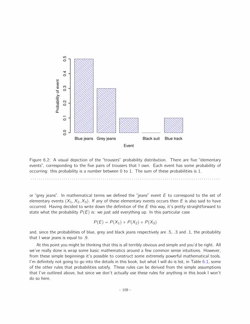
Blue jeans Grey jeans Black suit Blue track

Event

Pro

ba

bili

ty o

f eve

nt

0.0

0.1

0.2

0.3

0.4

0.5

Figure 6.2: A visual depiction of the “trousers” probability distribution. There are five “elementaryevents”, corresponding to the five pairs of trousers that I own. Each event has some probability ofoccurring: this probability is a number between 0 to 1. The sum of these probabilities is 1.

. . . . . . . . . . . . . . . . . . . . . . . . . . . . . . . . . . . . . . . . . . . . . . . . . . . . . . . . . . . . . . . . . . . . . . . . . . . . . . . . . . . . . . . . . . . .

or “grey jeans”. In mathematical terms we defined the “jeans” event E to correspond to the set ofelementary events pX1, X2, X3q. If any of these elementary events occurs then E is also said to haveoccurred. Having decided to write down the definition of the E this way, it’s pretty straightforward tostate what the probability P pEq is: we just add everything up. In this particular case

P pEq “ P pX1q ` P pX2q ` P pX3q

and, since the probabilities of blue, grey and black jeans respectively are .5, .3 and .1, the probabilitythat I wear jeans is equal to .9.

At this point you might be thinking that this is all terribly obvious and simple and you’d be right. Allwe’ve really done is wrap some basic mathematics around a few common sense intuitions. However,from these simple beginnings it’s possible to construct some extremely powerful mathematical tools.I’m definitely not going to go into the details in this book, but what I will do is list, in Table 6.1, someof the other rules that probabilities satisfy. These rules can be derived from the simple assumptionsthat I’ve outlined above, but since we don’t actually use these rules for anything in this book I won’tdo so here.

- 108 -

Table 6.1: Some basic rules that probabilities must satisfy. You don’t really need to know these rulesin order to understand the analyses that we’ll talk about later in the book, but they are important ifyou want to understand probability theory a bit more deeply.

English Notation Formulanot A P p Aq “ 1´ P pAq

A or B P pAY Bq “ P pAq ` P pBq ´ P pAX Bq

A and B P pAX Bq “ P pA|BqP pBq

. . . . . . . . . . . . . . . . . . . . . . . . . . . . . . . . . . . . . . . . . . . . . . . . . . . . . . . . . . . . . . . . . . . . . . . . . . . . . . . . . . . . . . . . . . . .

6.4

The binomial distribution

As you might imagine, probability distributions vary enormously and there’s an enormous range ofdistributions out there. However, they aren’t all equally important. In fact, the vast majority ofthe content in this book relies on one of five distributions: the binomial distribution, the normaldistribution, the t distribution, the χ2 (“chi-square”) distribution and the F distribution. Given this,what I’ll do over the next few sections is provide a brief introduction to all five of these, paying specialattention to the binomial and the normal. I’ll start with the binomial distribution since it’s the simplestof the five.

6.4.1 Introducing the binomial

The theory of probability originated in the attempt to describe how games of chance work, so it seemsfitting that our discussion of the binomial distribution should involve a discussion of rolling dice andflipping coins. Let’s imagine a simple “experiment”. In my hot little hand I’m holding 20 identicalsix-sided dice. On one face of each die there’s a picture of a skull, the other five faces are all blank.If I proceed to roll all 20 dice, what’s the probability that I’ll get exactly 4 skulls? Assuming that thedice are fair, we know that the chance of any one die coming up skulls is 1 in 6. To say this anotherway, the skull probability for a single die is approximately .167. This is enough information to answerour question, so let’s have a look at how it’s done.

As usual, we’ll want to introduce some names and some notation. We’ll let N denote the numberof dice rolls in our experiment, which is often referred to as the size parameter of our binomialdistribution. We’ll also use θ to refer to the the probability that a single die comes up skulls, a

- 109 -

Table 6.2: Formulas for the binomial and normal distributions. We don’t really use these formulasfor anything in this book, but they’re pretty important for more advanced work, so I thought it mightbe best to put them here in a table, where they can’t get in the way of the text. In the equationfor the binomial, X! is the factorial function (i.e., multiply all whole numbers from 1 to X), and forthe normal distribution “exp” refers to the exponential function. If these equations don’t make a lotof sense to you, don’t worry too much about them.

Binomial Normal

P pX | θ, Nq “N!

X!pN ´Xq!θXp1´ θqN´X ppX | µ, σq “

1?

2πσexp

ˆ

´pX ´ µq2

2σ2

˙

quantity that is usually called the success probability of the binomial.2 Finally, we’ll use X to referto the results of our experiment, namely the number of skulls I get when I roll the dice. Since theactual value of X is due to chance we refer to it as a random variable. In any case, now that wehave all this terminology and notation we can use it to state the problem a little more precisely. Thequantity that we want to calculate is the probability that X “ 4 given that we know that θ “ .167

and N “ 20. The general “form” of the thing I’m interested in calculating could be written as

P pX | θ, Nq

and we’re interested in the special case where X “ 4, θ “ .167 and N “ 20. There’s only one morepiece of notation I want to refer to before moving on to discuss the solution to the problem. If Iwant to say that X is generated randomly from a binomial distribution with parameters θ and N, thenotation I would use is as follows:

X „ Binomialpθ, Nq

Yeah, yeah. I know what you’re thinking: notation, notation, notation. Really, who cares? Very fewreaders of this book are here for the notation, so I should probably move on and talk about how touse the binomial distribution. I’ve included the formula for the binomial distribution in Table 6.2, sincesome readers may want to play with it themselves, but since most people probably don’t care thatmuch and because we don’t need the formula in this book, I won’t talk about it in any detail. Instead,I just want to show you what the binomial distribution looks like.

To that end, Figure 6.3 plots the binomial probabilities for all possible values of X for our dicerolling experiment, from X “ 0 (no skulls) all the way up to X “ 20 (all skulls). Note that this isbasically a bar chart, and is no different to the “trousers probability” plot I drew in Figure 6.2. On thehorizontal axis we have all the possible events, and on the vertical axis we can read off the probabilityof each of those events. So, the probability of rolling 4 skulls out of 20 is about 0.20 (the actual

2Note that the term “success” is pretty arbitrary and doesn’t actually imply that the outcome is something to bedesired. If θ referred to the probability that any one passenger gets injured in a bus crash I’d still call it the successprobability, but that doesn’t mean I want people to get hurt in bus crashes!

- 110 -

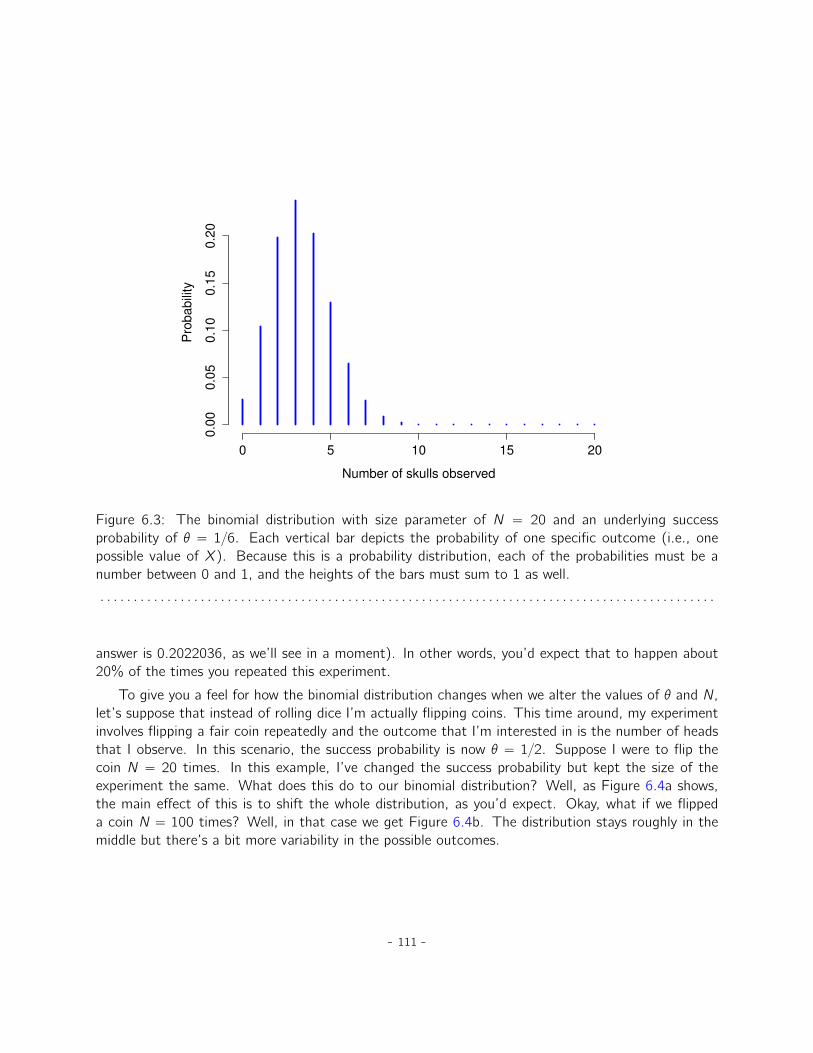
0 5 10 15 20

0.0

00

.05

0.1

00

.15

0.2

0

Number of skulls observed

Pro

ba

bili

ty

Figure 6.3: The binomial distribution with size parameter of N “ 20 and an underlying successprobability of θ “ 1{6. Each vertical bar depicts the probability of one specific outcome (i.e., onepossible value of X). Because this is a probability distribution, each of the probabilities must be anumber between 0 and 1, and the heights of the bars must sum to 1 as well.

. . . . . . . . . . . . . . . . . . . . . . . . . . . . . . . . . . . . . . . . . . . . . . . . . . . . . . . . . . . . . . . . . . . . . . . . . . . . . . . . . . . . . . . . . . . .

answer is 0.2022036, as we’ll see in a moment). In other words, you’d expect that to happen about20% of the times you repeated this experiment.

To give you a feel for how the binomial distribution changes when we alter the values of θ and N,let’s suppose that instead of rolling dice I’m actually flipping coins. This time around, my experimentinvolves flipping a fair coin repeatedly and the outcome that I’m interested in is the number of headsthat I observe. In this scenario, the success probability is now θ “ 1{2. Suppose I were to flip thecoin N “ 20 times. In this example, I’ve changed the success probability but kept the size of theexperiment the same. What does this do to our binomial distribution? Well, as Figure 6.4a shows,the main effect of this is to shift the whole distribution, as you’d expect. Okay, what if we flippeda coin N “ 100 times? Well, in that case we get Figure 6.4b. The distribution stays roughly in themiddle but there’s a bit more variability in the possible outcomes.

- 111 -

(a)

0 5 10 15 20

0.0

00

.05

0.1

00

.15

Number of heads observed

Pro

ba

bili

ty

(b)

0 20 40 60 80 100

0.0

00

.02

0.0

40

.06

0.0

8

Number of heads observed

Pro

ba

bili

ty

Figure 6.4: Two binomial distributions, involving a scenario in which I’m flipping a fair coin, so theunderlying success probability is θ “ 1{2. In panel (a), we assume I’m flipping the coin N “ 20 times.In panel (b) we assume that the coin is flipped N “ 100 times.

. . . . . . . . . . . . . . . . . . . . . . . . . . . . . . . . . . . . . . . . . . . . . . . . . . . . . . . . . . . . . . . . . . . . . . . . . . . . . . . . . . . . . . . . . . . .- 112 -

−3 −2 −1 0 1 2 3

0.0

0.1

0.2

0.3

0.4

Observed Value

Pro

ba

bili

ty D

en

sity

Figure 6.5: The normal distribution with mean µ “ 0 and standard deviation σ “ 1. The x-axiscorresponds to the value of some variable, and the y -axis tells us something about how likely weare to observe that value. However, notice that the y -axis is labelled “Probability Density” and not“Probability”. There is a subtle and somewhat frustrating characteristic of continuous distributionsthat makes the y axis behave a bit oddly: the height of the curve here isn’t actually the probabilityof observing a particular x value. On the other hand, it is true that the heights of the curve tells youwhich x values are more likely (the higher ones!). (see Section 6.5.1 for all the annoying details)

. . . . . . . . . . . . . . . . . . . . . . . . . . . . . . . . . . . . . . . . . . . . . . . . . . . . . . . . . . . . . . . . . . . . . . . . . . . . . . . . . . . . . . . . . . . .

6.5

The normal distribution

While the binomial distribution is conceptually the simplest distribution to understand, it’s not themost important one. That particular honour goes to the normal distribution, also referred to as “thebell curve” or a “Gaussian distribution”. A normal distribution is described using two parameters: themean of the distribution µ and the standard deviation of the distribution σ.

The notation that we sometimes use to say that a variable X is normally distributed is as follows:

X „ Normalpµ, σq

- 113 -

0 2 4 6 8 10

0.0

0.1

0.2

0.3

0.4

Observed Value

Pro

ba

bili

ty D

en

sity

Figure 6.6: An illustration of what happens when you change the mean of a normal distribution.The solid line depicts a normal distribution with a mean of µ “ 4. The dashed line shows a normaldistribution with a mean of µ “ 7. In both cases, the standard deviation is σ “ 1. Not surprisingly,the two distributions have the same shape, but the dashed line is shifted to the right.

. . . . . . . . . . . . . . . . . . . . . . . . . . . . . . . . . . . . . . . . . . . . . . . . . . . . . . . . . . . . . . . . . . . . . . . . . . . . . . . . . . . . . . . . . . . .

Of course, that’s just notation. It doesn’t tell us anything interesting about the normal distributionitself. As was the case with the binomial distribution, I have included the formula for the normaldistribution in this book, because I think it’s important enough that everyone who learns statisticsshould at least look at it, but since this is an introductory text I don’t want to focus on it, so I’vetucked it away in Table 6.2.

Instead of focusing on the maths, let’s try to get a sense for what it means for a variable to benormally distributed. To that end, have a look at Figure 6.5 which plots a normal distribution withmean µ “ 0 and standard deviation σ “ 1. You can see where the name “bell curve” comes from; itlooks a bit like a bell. Notice that, unlike the plots that I drew to illustrate the binomial distribution,the picture of the normal distribution in Figure 6.5 shows a smooth curve instead of “histogram-like”bars. This isn’t an arbitrary choice, the normal distribution is continuous whereas the binomial isdiscrete. For instance, in the die rolling example from the last section it was possible to get 3 skullsor 4 skulls, but impossible to get 3.9 skulls. The figures that I drew in the previous section reflectedthis fact. In Figure 6.3, for instance, there’s a bar located at X “ 3 and another one at X “ 4 but

- 114 -

0 2 4 6 8 10

0.0

0.1

0.2

0.3

0.4

Observed Value

Pro

ba

bili

ty D

en

sity

Figure 6.7: An illustration of what happens when you change the the standard deviation of a normaldistribution. Both distributions plotted in this figure have a mean of µ “ 5, but they have differentstandard deviations. The solid line plots a distribution with standard deviation σ “ 1, and the dashedline shows a distribution with standard deviation σ “ 2. As a consequence, both distributions are“centred” on the same spot, but the dashed line is wider than the solid one.

. . . . . . . . . . . . . . . . . . . . . . . . . . . . . . . . . . . . . . . . . . . . . . . . . . . . . . . . . . . . . . . . . . . . . . . . . . . . . . . . . . . . . . . . . . . .

there’s nothing in between. Continuous quantities don’t have this constraint. For instance, supposewe’re talking about the weather. The temperature on a pleasant Spring day could be 23 degrees, 24degrees, 23.9 degrees, or anything in between since temperature is a continuous variable. And so anormal distribution might be quite appropriate for describing Spring temperatures.3

With this in mind, let’s see if we can’t get an intuition for how the normal distribution works. First,let’s have a look at what happens when we play around with the parameters of the distribution. Tothat end, Figure 6.6 plots normal distributions that have different means but have the same standarddeviation. As you might expect, all of these distributions have the same “width”. The only differencebetween them is that they’ve been shifted to the left or to the right. In every other respect they’reidentical. In contrast, if we increase the standard deviation while keeping the mean constant, the

3In practice, the normal distribution is so handy that people tend to use it even when the variable isn’t actuallycontinuous. As long as there are enough categories (e.g., Likert scale responses to a questionnaire), it’s pretty standardpractice to use the normal distribution as an approximation. This works out much better in practice than you’d think.

- 115 -

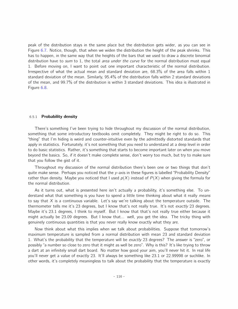
peak of the distribution stays in the same place but the distribution gets wider, as you can see inFigure 6.7. Notice, though, that when we widen the distribution the height of the peak shrinks. Thishas to happen, in the same way that the heights of the bars that we used to draw a discrete binomialdistribution have to sum to 1, the total area under the curve for the normal distribution must equal1. Before moving on, I want to point out one important characteristic of the normal distribution.Irrespective of what the actual mean and standard deviation are, 68.3% of the area falls within 1standard deviation of the mean. Similarly, 95.4% of the distribution falls within 2 standard deviationsof the mean, and 99.7% of the distribution is within 3 standard deviations. This idea is illustrated inFigure 6.8.

6.5.1 Probability density

There’s something I’ve been trying to hide throughout my discussion of the normal distribution,something that some introductory textbooks omit completely. They might be right to do so. This“thing” that I’m hiding is weird and counter-intuitive even by the admittedly distorted standards thatapply in statistics. Fortunately, it’s not something that you need to understand at a deep level in orderto do basic statistics. Rather, it’s something that starts to become important later on when you movebeyond the basics. So, if it doesn’t make complete sense, don’t worry too much, but try to make surethat you follow the gist of it.

Throughout my discussion of the normal distribution there’s been one or two things that don’tquite make sense. Perhaps you noticed that the y -axis in these figures is labelled “Probability Density”rather than density. Maybe you noticed that I used ppXq instead of P pXq when giving the formula forthe normal distribution.

As it turns out, what is presented here isn’t actually a probability, it’s something else. To un-derstand what that something is you have to spend a little time thinking about what it really meansto say that X is a continuous variable. Let’s say we’re talking about the temperature outside. Thethermometer tells me it’s 23 degrees, but I know that’s not really true. It’s not exactly 23 degrees.Maybe it’s 23.1 degrees, I think to myself. But I know that that’s not really true either because itmight actually be 23.09 degrees. But I know that... well, you get the idea. The tricky thing withgenuinely continuous quantities is that you never really know exactly what they are.

Now think about what this implies when we talk about probabilities. Suppose that tomorrow’smaximum temperature is sampled from a normal distribution with mean 23 and standard deviation1. What’s the probability that the temperature will be exactly 23 degrees? The answer is “zero”, orpossibly “a number so close to zero that it might as well be zero”. Why is this? It’s like trying to throwa dart at an infinitely small dart board. No matter how good your aim, you’ll never hit it. In real lifeyou’ll never get a value of exactly 23. It’ll always be something like 23.1 or 22.99998 or suchlike. Inother words, it’s completely meaningless to talk about the probability that the temperature is exactly

- 116 -

−4 −3 −2 −1 0 1 2 3 4

Shaded Area = 68.3%

−4 −3 −2 −1 0 1 2 3 4

Shaded Area = 95.4%

(a) (b)

Figure 6.8: The area under the curve tells you the probability that an observation falls within aparticular range. The solid lines plot normal distributions with mean µ “ 0 and standard deviationσ “ 1. The shaded areas illustrate “areas under the curve” for two important cases. In panel a, wecan see that there is a 68.3% chance that an observation will fall within one standard deviation ofthe mean. In panel b, we see that there is a 95.4% chance that an observation will fall within twostandard deviations of the mean.

. . . . . . . . . . . . . . . . . . . . . . . . . . . . . . . . . . . . . . . . . . . . . . . . . . . . . . . . . . . . . . . . . . . . . . . . . . . . . . . . . . . . . . . . . . . .

−4 −3 −2 −1 0 1 2 3 4

Shaded Area = 15.9%

−4 −3 −2 −1 0 1 2 3 4

Shaded Area = 34.1%

(a) (b)

Figure 6.9: Two more examples of the “area under the curve idea”. There is a 15.9% chance that anobservation is one standard deviation below the mean or smaller (panel a), and a 34.1% chance thatthe observation is somewhere between one standard deviation below the mean and the mean (panelb). Notice that if you add these two numbers together you get 15.9%` 34.1% “ 50%. For normallydistributed data, there is a 50% chance that an observation falls below the mean. And of course thatalso implies that there is a 50% chance that it falls above the mean.

. . . . . . . . . . . . . . . . . . . . . . . . . . . . . . . . . . . . . . . . . . . . . . . . . . . . . . . . . . . . . . . . . . . . . . . . . . . . . . . . . . . . . . . . . . . .

- 117 -

23 degrees. However, in everyday language if I told you that it was 23 degrees outside and it turnedout to be 22.9998 degrees you probably wouldn’t call me a liar. Because in everyday language “23degrees” usually means something like “somewhere between 22.5 and 23.5 degrees”. And while itdoesn’t feel very meaningful to ask about the probability that the temperature is exactly 23 degrees,it does seem sensible to ask about the probability that the temperature lies between 22.5 and 23.5,or between 20 and 30, or any other range of temperatures.

The point of this discussion is to make clear that when we’re talking about continuous distributionsit’s not meaningful to talk about the probability of a specific value. However, what we can talk aboutis the probability that the value lies within a particular range of values. To find out the probabilityassociated with a particular range what you need to do is calculate the “area under the curve”. We’veseen this concept already, in Figure 6.8 the shaded areas shown depict genuine probabilities (e.g., inFigure 6.8a it shows the probability of observing a value that falls within 1 standard deviation of themean).

Okay, so that explains part of the story. I’ve explained a little bit about how continuous probabilitydistributions should be interpreted (i.e., area under the curve is the key thing). But what does theformula for ppxq that I described earlier actually mean? Obviously, ppxq doesn’t describe a probability,but what is it? The name for this quantity ppxq is a probability density, and in terms of the plots we’vebeen drawing it corresponds to the height of the curve. The densities themselves aren’t meaningful inand of themselves, but they’re “rigged” to ensure that the area under the curve is always interpretableas genuine probabilities. To be honest, that’s about as much as you really need to know for now.4

6.6

Other useful distributions

The normal distribution is the distribution that statistics makes most use of (for reasons to be discussedshortly), and the binomial distribution is a very useful one for lots of purposes. But the world ofstatistics is filled with probability distributions, some of which we’ll run into in passing. In particular,the three that will appear in this book are the t distribution, the χ2 distribution and the F distribution.I won’t give formulas for any of these, or talk about them in too much detail, but I will show you somepictures.

4For those readers who know a little calculus, I’ll give a slightly more precise explanation. In the same way thatprobabilities are non-negative numbers that must sum to 1, probability densities are non-negative numbers that mustintegrate to 1 (where the integral is taken across all possible values of X). To calculate the probability that X fallsbetween a and b we calculate the definite integral of the density function over the corresponding range,

şb

appxq dx . If

you don’t remember or never learned calculus, don’t worry about this. It’s not needed for this book.

- 118 -

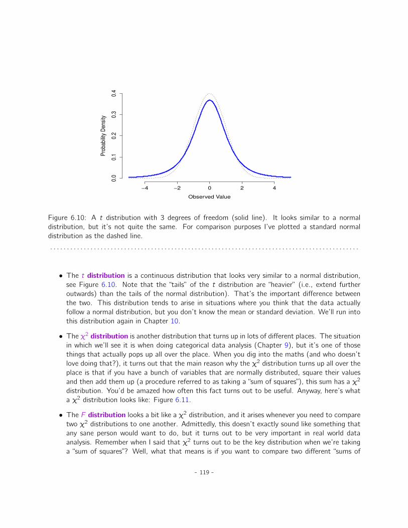
−4 −2 0 2 4

0.0

0.1

0.2

0.3

0.4

Observed Value

Pro

babi

lity

Den

sity

Figure 6.10: A t distribution with 3 degrees of freedom (solid line). It looks similar to a normaldistribution, but it’s not quite the same. For comparison purposes I’ve plotted a standard normaldistribution as the dashed line.

. . . . . . . . . . . . . . . . . . . . . . . . . . . . . . . . . . . . . . . . . . . . . . . . . . . . . . . . . . . . . . . . . . . . . . . . . . . . . . . . . . . . . . . . . . . .

• The t distribution is a continuous distribution that looks very similar to a normal distribution,see Figure 6.10. Note that the “tails” of the t distribution are “heavier” (i.e., extend furtheroutwards) than the tails of the normal distribution). That’s the important difference betweenthe two. This distribution tends to arise in situations where you think that the data actuallyfollow a normal distribution, but you don’t know the mean or standard deviation. We’ll run intothis distribution again in Chapter 10.

• The χ2 distribution is another distribution that turns up in lots of different places. The situationin which we’ll see it is when doing categorical data analysis (Chapter 9), but it’s one of thosethings that actually pops up all over the place. When you dig into the maths (and who doesn’tlove doing that?), it turns out that the main reason why the χ2 distribution turns up all over theplace is that if you have a bunch of variables that are normally distributed, square their valuesand then add them up (a procedure referred to as taking a “sum of squares”), this sum has a χ2

distribution. You’d be amazed how often this fact turns out to be useful. Anyway, here’s whata χ2 distribution looks like: Figure 6.11.

• The F distribution looks a bit like a χ2 distribution, and it arises whenever you need to comparetwo χ2 distributions to one another. Admittedly, this doesn’t exactly sound like something thatany sane person would want to do, but it turns out to be very important in real world dataanalysis. Remember when I said that χ2 turns out to be the key distribution when we’re takinga “sum of squares”? Well, what that means is if you want to compare two different “sums of

- 119 -

0 2 4 6 8 10

0.0

00.0

50.1

00.1

50.2

00.2

5

Observed Value

Pro

babili

ty D

ensity

Figure 6.11: A χ2 distribution with 3 degrees of freedom. Notice that the observed values mustalways be greater than zero, and that the distribution is pretty skewed. These are the key features ofa chi-square distribution.

. . . . . . . . . . . . . . . . . . . . . . . . . . . . . . . . . . . . . . . . . . . . . . . . . . . . . . . . . . . . . . . . . . . . . . . . . . . . . . . . . . . . . . . . . . . .

- 120 -

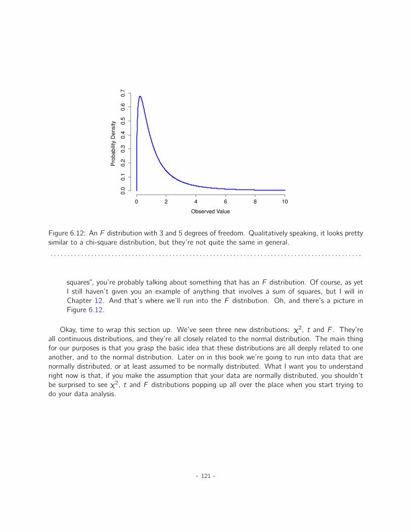
0 2 4 6 8 10

0.0

0.1

0.2

0.3

0.4

0.5

0.6

0.7

Observed Value

Pro

babili

ty D

ensity

Figure 6.12: An F distribution with 3 and 5 degrees of freedom. Qualitatively speaking, it looks prettysimilar to a chi-square distribution, but they’re not quite the same in general.

. . . . . . . . . . . . . . . . . . . . . . . . . . . . . . . . . . . . . . . . . . . . . . . . . . . . . . . . . . . . . . . . . . . . . . . . . . . . . . . . . . . . . . . . . . . .

squares”, you’re probably talking about something that has an F distribution. Of course, as yetI still haven’t given you an example of anything that involves a sum of squares, but I will inChapter 12. And that’s where we’ll run into the F distribution. Oh, and there’s a picture inFigure 6.12.

Okay, time to wrap this section up. We’ve seen three new distributions: χ2, t and F . They’reall continuous distributions, and they’re all closely related to the normal distribution. The main thingfor our purposes is that you grasp the basic idea that these distributions are all deeply related to oneanother, and to the normal distribution. Later on in this book we’re going to run into data that arenormally distributed, or at least assumed to be normally distributed. What I want you to understandright now is that, if you make the assumption that your data are normally distributed, you shouldn’tbe surprised to see χ2, t and F distributions popping up all over the place when you start trying todo your data analysis.

- 121 -

6.7

Summary

In this chapter we’ve talked about probability. We’ve talked about what probability means and whystatisticians can’t agree on what it means. We talked about the rules that probabilities have to obey.And we introduced the idea of a probability distribution and spent a good chunk of the chapter talkingabout some of the more important probability distributions that statisticians work with. The sectionby section breakdown looks like this:

• Probability theory versus statistics (Section 6.1)

• Frequentist versus Bayesian views of probability (Section 6.2)

• Basics of probability theory (Section 6.3)

• Binomial distribution (Section 6.4), normal distribution (Section 6.5), and others (Section 6.6)

As you’d expect, my coverage is by no means exhaustive. Probability theory is a large branch ofmathematics in its own right, entirely separate from its application to statistics and data analysis.As such, there are thousands of books written on the subject and universities generally offer multipleclasses devoted entirely to probability theory. Even the “simpler” task of documenting standard prob-ability distributions is a big topic. I’ve described five standard probability distributions in this chapter,but sitting on my bookshelf I have a 45-chapter book called “Statistical Distributions” (Evans, Hast-ings, and Peacock 2011) that lists a lot more than that. Fortunately for you, very little of this isnecessary. You’re unlikely to need to know dozens of statistical distributions when you go out and doreal world data analysis, and you definitely won’t need them for this book, but it never hurts to knowthat there’s other possibilities out there.

Picking up on that last point, there’s a sense in which this whole chapter is something of adigression. Many undergraduate psychology classes on statistics skim over this content very quickly (Iknow mine did), and even the more advanced classes will often “forget” to revisit the basic foundationsof the field. Most academic psychologists would not know the difference between probability anddensity, and until recently very few would have been aware of the difference between Bayesian andfrequentist probability. However, I think it’s important to understand these things before moving ontothe applications. For example, there are a lot of rules about what you’re “allowed” to say when doingstatistical inference and many of these can seem arbitrary and weird. However, they start to makesense if you understand that there is this Bayesian/frequentist distinction. Similarly, in Chapter 10we’re going to talk about something called the t-test, and if you really want to have a grasp of themechanics of the t-test it really helps to have a sense of what a t-distribution actually looks like. Youget the idea, I hope.

- 122 -

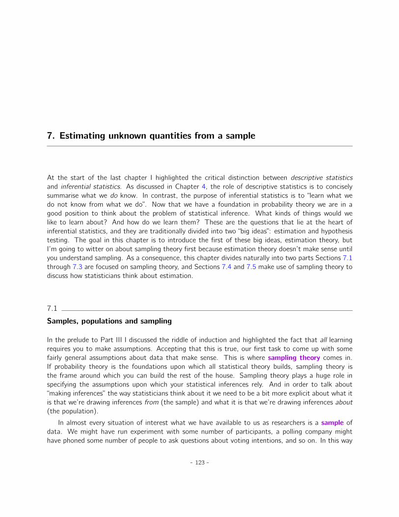
7. Estimating unknown quantities from a sample

At the start of the last chapter I highlighted the critical distinction between descriptive statisticsand inferential statistics. As discussed in Chapter 4, the role of descriptive statistics is to conciselysummarise what we do know. In contrast, the purpose of inferential statistics is to “learn what wedo not know from what we do”. Now that we have a foundation in probability theory we are in agood position to think about the problem of statistical inference. What kinds of things would welike to learn about? And how do we learn them? These are the questions that lie at the heart ofinferential statistics, and they are traditionally divided into two “big ideas”: estimation and hypothesistesting. The goal in this chapter is to introduce the first of these big ideas, estimation theory, butI’m going to witter on about sampling theory first because estimation theory doesn’t make sense untilyou understand sampling. As a consequence, this chapter divides naturally into two parts Sections 7.1through 7.3 are focused on sampling theory, and Sections 7.4 and 7.5 make use of sampling theory todiscuss how statisticians think about estimation.

7.1

Samples, populations and sampling

In the prelude to Part III I discussed the riddle of induction and highlighted the fact that all learningrequires you to make assumptions. Accepting that this is true, our first task to come up with somefairly general assumptions about data that make sense. This is where sampling theory comes in.If probability theory is the foundations upon which all statistical theory builds, sampling theory isthe frame around which you can build the rest of the house. Sampling theory plays a huge role inspecifying the assumptions upon which your statistical inferences rely. And in order to talk about“making inferences” the way statisticians think about it we need to be a bit more explicit about what itis that we’re drawing inferences from (the sample) and what it is that we’re drawing inferences about(the population).

In almost every situation of interest what we have available to us as researchers is a sample ofdata. We might have run experiment with some number of participants, a polling company mighthave phoned some number of people to ask questions about voting intentions, and so on. In this way

- 123 -

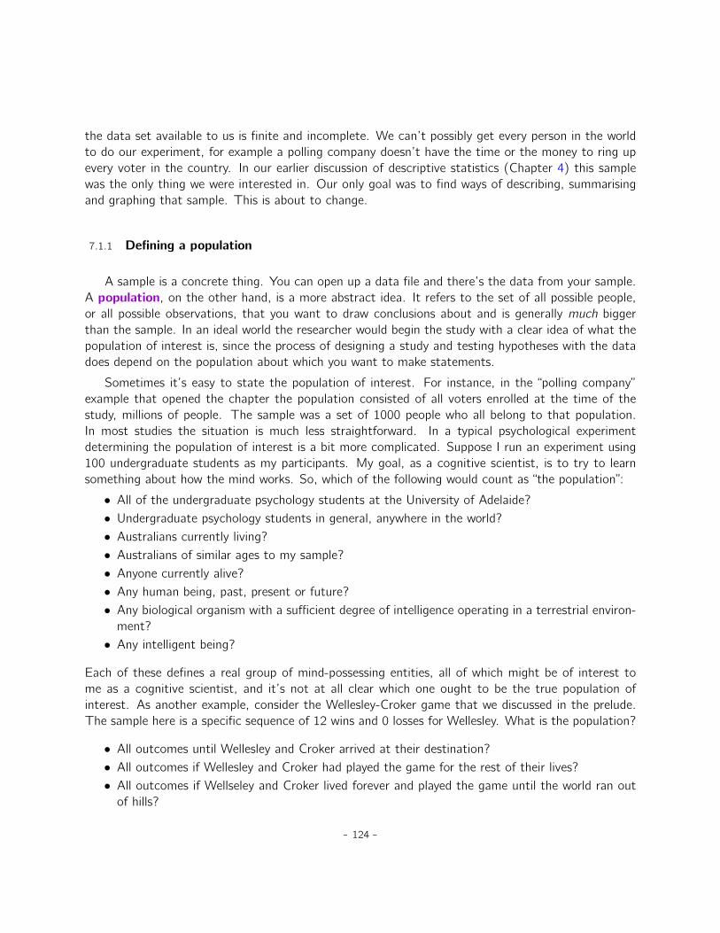
the data set available to us is finite and incomplete. We can’t possibly get every person in the worldto do our experiment, for example a polling company doesn’t have the time or the money to ring upevery voter in the country. In our earlier discussion of descriptive statistics (Chapter 4) this samplewas the only thing we were interested in. Our only goal was to find ways of describing, summarisingand graphing that sample. This is about to change.

7.1.1 Defining a population

A sample is a concrete thing. You can open up a data file and there’s the data from your sample.A population, on the other hand, is a more abstract idea. It refers to the set of all possible people,or all possible observations, that you want to draw conclusions about and is generally much biggerthan the sample. In an ideal world the researcher would begin the study with a clear idea of what thepopulation of interest is, since the process of designing a study and testing hypotheses with the datadoes depend on the population about which you want to make statements.

Sometimes it’s easy to state the population of interest. For instance, in the “polling company”example that opened the chapter the population consisted of all voters enrolled at the time of thestudy, millions of people. The sample was a set of 1000 people who all belong to that population.In most studies the situation is much less straightforward. In a typical psychological experimentdetermining the population of interest is a bit more complicated. Suppose I run an experiment using100 undergraduate students as my participants. My goal, as a cognitive scientist, is to try to learnsomething about how the mind works. So, which of the following would count as “the population”:

• All of the undergraduate psychology students at the University of Adelaide?• Undergraduate psychology students in general, anywhere in the world?• Australians currently living?• Australians of similar ages to my sample?• Anyone currently alive?• Any human being, past, present or future?• Any biological organism with a sufficient degree of intelligence operating in a terrestrial environ-ment?• Any intelligent being?

Each of these defines a real group of mind-possessing entities, all of which might be of interest tome as a cognitive scientist, and it’s not at all clear which one ought to be the true population ofinterest. As another example, consider the Wellesley-Croker game that we discussed in the prelude.The sample here is a specific sequence of 12 wins and 0 losses for Wellesley. What is the population?

• All outcomes until Wellesley and Croker arrived at their destination?• All outcomes if Wellesley and Croker had played the game for the rest of their lives?• All outcomes if Wellseley and Croker lived forever and played the game until the world ran outof hills?

- 124 -

Figure 7.1: Simple random sampling without replacement from a finite population

. . . . . . . . . . . . . . . . . . . . . . . . . . . . . . . . . . . . . . . . . . . . . . . . . . . . . . . . . . . . . . . . . . . . . . . . . . . . . . . . . . . . . . . . . . . .

• All outcomes if we created an infinite set of parallel universes and the Wellesely/Croker pairmade guesses about the same 12 hills in each universe?

Again, it’s not obvious what the population is.

7.1.2 Simple random samples

Irrespective of how I define the population, the critical point is that the sample is a subset of thepopulation and our goal is to use our knowledge of the sample to draw inferences about the propertiesof the population. The relationship between the two depends on the procedure by which the samplewas selected. This procedure is referred to as a sampling method and it is important to understandwhy it matters.

To keep things simple, let’s imagine that we have a bag containing 10 chips. Each chip has aunique letter printed on it so we can distinguish between the 10 chips. The chips come in two colours,black and white. This set of chips is the population of interest and it is depicted graphically on theleft of Figure 7.1. As you can see from looking at the picture there are 4 black chips and 6 whitechips, but of course in real life we wouldn’t know that unless we looked in the bag. Now imagine yourun the following “experiment”: you shake up the bag, close your eyes, and pull out 4 chips withoutputting any of them back into the bag. First out comes the a chip (black), then the c chip (white),then j (white) and then finally b (black). If you wanted you could then put all the chips back in thebag and repeat the experiment, as depicted on the right hand side of Figure 7.1. Each time you getdifferent results but the procedure is identical in each case. The fact that the same procedure can

- 125 -

Figure 7.2: Biased sampling without replacement from a finite population

. . . . . . . . . . . . . . . . . . . . . . . . . . . . . . . . . . . . . . . . . . . . . . . . . . . . . . . . . . . . . . . . . . . . . . . . . . . . . . . . . . . . . . . . . . . .

lead to different results each time we refer to as a random process.1 However, because we shook thebag before pulling any chips out, it seems reasonable to think that every chip has the same chanceof being selected. A procedure in which every member of the population has the same chance ofbeing selected is called a simple random sample. The fact that we did not put the chips back in thebag after pulling them out means that you can’t observe the same thing twice, and in such cases theobservations are said to have been sampled without replacement.

To help make sure you understand the importance of the sampling procedure, consider an alter-native way in which the experiment could have been run. Suppose that my 5-year old son had openedthe bag and decided to pull out four black chips without putting any of them back in the bag. Thisbiased sampling scheme is depicted in Figure 7.2. Now consider the evidential value of seeing 4 blackchips and 0 white chips. Clearly it depends on the sampling scheme, does it not? If you know that thesampling scheme is biased to select only black chips then a sample that consists of only black chipsdoesn’t tell you very much about the population! For this reason statisticians really like it when a dataset can be considered a simple random sample, because it makes the data analysis much easier.

A third procedure is worth mentioning. This time around we close our eyes, shake the bag, andpull out a chip. This time, however, we record the observation and then put the chip back in thebag. Again we close our eyes, shake the bag, and pull out a chip. We then repeat this procedureuntil we have 4 chips. Data sets generated in this way are still simple random samples, but becausewe put the chips back in the bag immediately after drawing them it is referred to as a sample withreplacement. The difference between this situation and the first one is that it is possible to observethe same population member multiple times, as illustrated in Figure 7.3.

In my experience, most psychology experiments tend to be sampling without replacement, because1The proper mathematical definition of randomness is extraordinarily technical, and way beyond the scope of this

book. We’ll be non-technical here and say that a process has an element of randomness to it whenever it is possible torepeat the process and get different answers each time.

- 126 -

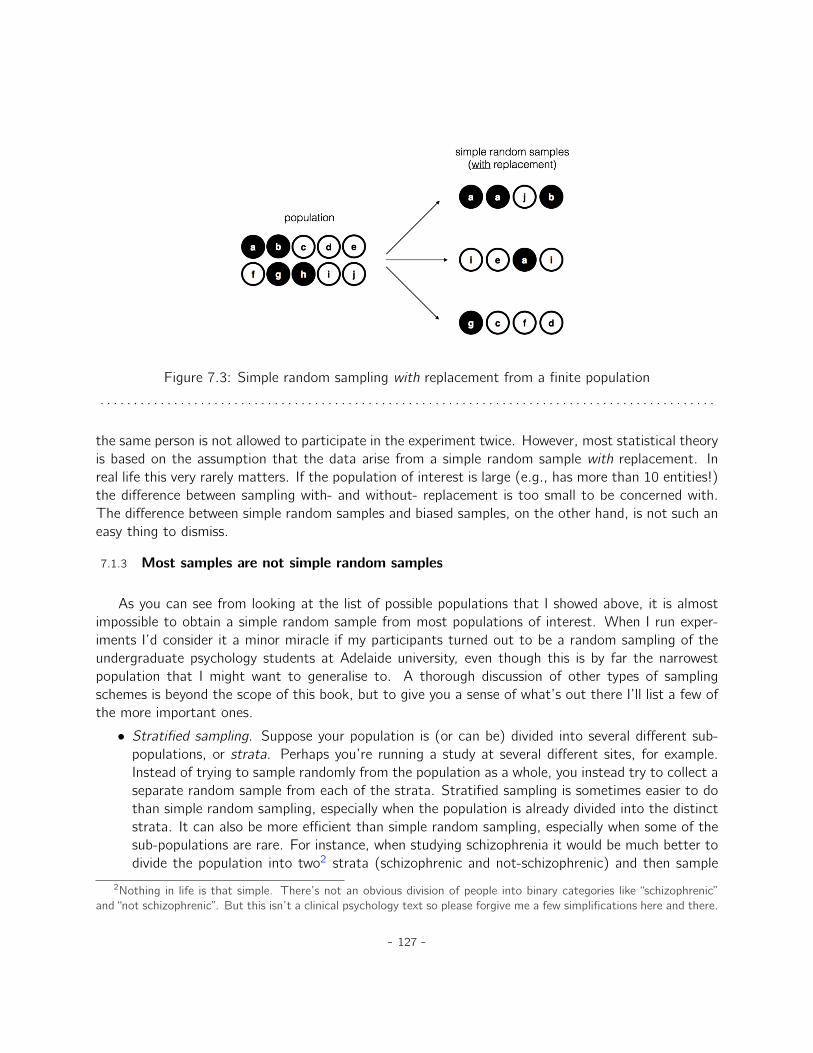
Figure 7.3: Simple random sampling with replacement from a finite population

. . . . . . . . . . . . . . . . . . . . . . . . . . . . . . . . . . . . . . . . . . . . . . . . . . . . . . . . . . . . . . . . . . . . . . . . . . . . . . . . . . . . . . . . . . . .

the same person is not allowed to participate in the experiment twice. However, most statistical theoryis based on the assumption that the data arise from a simple random sample with replacement. Inreal life this very rarely matters. If the population of interest is large (e.g., has more than 10 entities!)the difference between sampling with- and without- replacement is too small to be concerned with.The difference between simple random samples and biased samples, on the other hand, is not such aneasy thing to dismiss.

7.1.3 Most samples are not simple random samples

As you can see from looking at the list of possible populations that I showed above, it is almostimpossible to obtain a simple random sample from most populations of interest. When I run exper-iments I’d consider it a minor miracle if my participants turned out to be a random sampling of theundergraduate psychology students at Adelaide university, even though this is by far the narrowestpopulation that I might want to generalise to. A thorough discussion of other types of samplingschemes is beyond the scope of this book, but to give you a sense of what’s out there I’ll list a few ofthe more important ones.

• Stratified sampling. Suppose your population is (or can be) divided into several different sub-populations, or strata. Perhaps you’re running a study at several different sites, for example.Instead of trying to sample randomly from the population as a whole, you instead try to collect aseparate random sample from each of the strata. Stratified sampling is sometimes easier to dothan simple random sampling, especially when the population is already divided into the distinctstrata. It can also be more efficient than simple random sampling, especially when some of thesub-populations are rare. For instance, when studying schizophrenia it would be much better todivide the population into two2 strata (schizophrenic and not-schizophrenic) and then sample

2Nothing in life is that simple. There’s not an obvious division of people into binary categories like “schizophrenic”and “not schizophrenic”. But this isn’t a clinical psychology text so please forgive me a few simplifications here and there.

- 127 -

an equal number of people from each group. If you selected people randomly you would get sofew schizophrenic people in the sample that your study would be useless. This specific kind ofof stratified sampling is referred to as oversampling because it makes a deliberate attempt toover-represent rare groups.

• Snowball sampling is a technique that is especially useful when sampling from a “hidden” orhard to access population and is especially common in social sciences. For instance, supposethe researchers want to conduct an opinion poll among transgender people. The research teammight only have contact details for a few trans folks, so the survey starts by asking them toparticipate (stage 1). At the end of the survey the participants are asked to provide contactdetails for other people who might want to participate. In stage 2 those new contacts aresurveyed. The process continues until the researchers have sufficient data. The big advantageto snowball sampling is that it gets you data in situations that might otherwise be impossible toget any. On the statistical side, the main disadvantage is that the sample is highly non-random,and non-random in ways that are difficult to address. On the real life side, the disadvantage isthat the procedure can be unethical if not handled well, because hidden populations are oftenhidden for a reason. I chose transgender people as an example here to highlight this issue. Ifyou weren’t careful you might end up outing people who don’t want to be outed (very, verybad form), and even if you don’t make that mistake it can still be intrusive to use people’ssocial networks to study them. It’s certainly very hard to get people’s informed consent beforecontacting them, yet in many cases the simple act of contacting them and saying “hey we wantto study you” can be hurtful. Social networks are complex things, and just because you can usethem to get data doesn’t always mean you should.

• Convenience sampling is more or less what it sounds like. The samples are chosen in a way thatis convenient to the researcher, and not selected at random from the population of interest.Snowball sampling is one type of convenience sampling, but there are many others. A com-mon example in psychology are studies that rely on undergraduate psychology students. Thesesamples are generally non-random in two respects. First, reliance on undergraduate psychologystudents automatically means that your data are restricted to a single sub-population. Second,the students usually get to pick which studies they participate in, so the sample is a self selectedsubset of psychology students and not a randomly selected subset. In real life most studies areconvenience samples of one form or another. This is sometimes a severe limitation, but notalways.

7.1.4 How much does it matter if you don’t have a simple random sample?

Okay, so real world data collection tends not to involve nice simple random samples. Does thatmatter? A little thought should make it clear to you that it can matter if your data are not a simplerandom sample. Just think about the difference between Figures 7.1 and 7.2. However, it’s notquite as bad as it sounds. Some types of biased samples are entirely unproblematic. For instance,

- 128 -

when using a stratified sampling technique you actually know what the bias is because you createdit deliberately, often to increase the effectiveness of your study, and there are statistical techniquesthat you can use to adjust for the biases you’ve introduced (not covered in this book!). So in thosesituations it’s not a problem.

More generally though, it’s important to remember that random sampling is a means to an end,and not the end in itself. Let’s assume you’ve relied on a convenience sample, and as such you canassume it’s biased. A bias in your sampling method is only a problem if it causes you to draw thewrong conclusions. When viewed from that perspective, I’d argue that we don’t need the sample to berandomly generated in every respect, we only need it to be random with respect to the psychologically-relevant phenomenon of interest. Suppose I’m doing a study looking at working memory capacity. Instudy 1, I actually have the ability to sample randomly from all human beings currently alive, with oneexception: I can only sample people born on a Monday. In study 2, I am able to sample randomlyfrom the Australian population. I want to generalise my results to the population of all living humans.Which study is better? The answer, obviously, is study 1. Why? Because we have no reason tothink that being “born on a Monday” has any interesting relationship to working memory capacity. Incontrast, I can think of several reasons why “being Australian” might matter. Australia is a wealthy,industrialised country with a very well-developed education system. People growing up in that systemwill have had life experiences much more similar to the experiences of the people who designed thetests for working memory capacity. This shared experience might easily translate into similar beliefsabout how to “take a test”, a shared assumption about how psychological experimentation works, andso on. These things might actually matter. For instance, “test taking” style might have taught theAustralian participants how to direct their attention exclusively on fairly abstract test materials muchmore than people who haven’t grown up in a similar environment. This could therefore lead to amisleading picture of what working memory capacity is.

There are two points hidden in this discussion. First, when designing your own studies, it’s impor-tant to think about what population you care about and try hard to sample in a way that is appropriateto that population. In practice, you’re usually forced to put up with a “sample of convenience” (e.g.,psychology lecturers sample psychology students because that’s the least expensive way to collectdata, and our coffers aren’t exactly overflowing with gold), but if so you should at least spend sometime thinking about what the dangers of this practice might be. Second, if you’re going to criticisesomeone else’s study because they’ve used a sample of convenience rather than laboriously samplingrandomly from the entire human population, at least have the courtesy to offer a specific theory asto how this might have distorted the results.

7.1.5 Population parameters and sample statistics

Okay. Setting aside the thorny methodological issues associated with obtaining a random sample,let’s consider a slightly different issue. Up to this point we have been talking about populations theway a scientist might. To a psychologist a population might be a group of people. To an ecologista population might be a group of bears. In most cases the populations that scientists care about areconcrete things that actually exist in the real world. Statisticians, however, are a funny lot. On the one

- 129 -

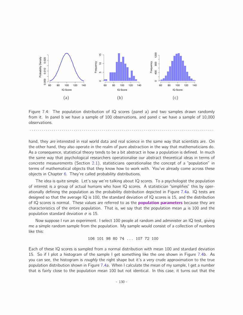
60 80 100 120 140

0.0

00

0.0

10

0.0

20

IQ Score

Pro

ba

bili

ty D

en

sity

IQ Score

Fre

qu

en

cy

60 80 100 120 140

05

10

15

IQ Score

Fre

qu

en

cy

60 80 100 120 140

04

00

80

01

20

0

(a) (b) (c)

Figure 7.4: The population distribution of IQ scores (panel a) and two samples drawn randomlyfrom it. In panel b we have a sample of 100 observations, and panel c we have a sample of 10,000observations.

. . . . . . . . . . . . . . . . . . . . . . . . . . . . . . . . . . . . . . . . . . . . . . . . . . . . . . . . . . . . . . . . . . . . . . . . . . . . . . . . . . . . . . . . . . . .

hand, they are interested in real world data and real science in the same way that scientists are. Onthe other hand, they also operate in the realm of pure abstraction in the way that mathematicians do.As a consequence, statistical theory tends to be a bit abstract in how a population is defined. In muchthe same way that psychological researchers operationalise our abstract theoretical ideas in terms ofconcrete measurements (Section 2.1), statisticians operationalise the concept of a “population” interms of mathematical objects that they know how to work with. You’ve already come across theseobjects in Chapter 6. They’re called probability distributions.

The idea is quite simple. Let’s say we’re talking about IQ scores. To a psychologist the populationof interest is a group of actual humans who have IQ scores. A statistician “simplifies” this by oper-ationally defining the population as the probability distribution depicted in Figure 7.4a. IQ tests aredesigned so that the average IQ is 100, the standard deviation of IQ scores is 15, and the distributionof IQ scores is normal. These values are referred to as the population parameters because they arecharacteristics of the entire population. That is, we say that the population mean µ is 100 and thepopulation standard deviation σ is 15.

Now suppose I run an experiment. I select 100 people at random and administer an IQ test, givingme a simple random sample from the population. My sample would consist of a collection of numberslike this:

106 101 98 80 74 ... 107 72 100

Each of these IQ scores is sampled from a normal distribution with mean 100 and standard deviation15. So if I plot a histogram of the sample I get something like the one shown in Figure 7.4b. Asyou can see, the histogram is roughly the right shape but it’s a very crude approximation to the truepopulation distribution shown in Figure 7.4a. When I calculate the mean of my sample, I get a numberthat is fairly close to the population mean 100 but not identical. In this case, it turns out that the

- 130 -

people in my sample have a mean IQ of 98.5, and the standard deviation of their IQ scores is 15.9.These sample statistics are properties of my data set, and although they are fairly similar to the truepopulation values they are not the same. In general, sample statistics are the things you can calculatefrom your data set and the population parameters are the things you want to learn about. Later on inthis chapter I’ll talk about how you can estimate population parameters using your sample statistics(Section 7.4) and how to work out how confident you are in your estimates (Section 7.5) but beforewe get to that there’s a few more ideas in sampling theory that you need to know about.

7.2

The law of large numbers

In the previous section I showed you the results of one fictitious IQ experiment with a sample sizeof N “ 100. The results were somewhat encouraging as the true population mean is 100 and thesample mean of 98.5 is a pretty reasonable approximation to it. In many scientific studies that levelof precision is perfectly acceptable, but in other situations you need to be a lot more precise. If wewant our sample statistics to be much closer to the population parameters, what can we do about it?

The obvious answer is to collect more data. Suppose that we ran a much larger experiment,this time measuring the IQs of 10,000 people. We can simulate the results of this experiment usingJASP. The IQsim.jasp file is a JASP data file. In this file I have generated 10,000 random numberssampled from a normal distribution for a population with mean = 100 and sd = 15. By the way, Idid this entirely within JASP computing a new variable using the R code rnorm(10000, 100, 15). Ahistogram and density plot shows that this larger sample is a much better approximation to the truepopulation distribution than the smaller one. This is reflected in the sample statistics. The mean IQfor the larger sample turns out to be 100.107 and the standard deviation is 14.995. These values arenow very close to the true population. See Figure 7.5

I feel a bit silly saying this, but the thing I want you to take away from this is that large samplesgenerally give you better information. I feel silly saying it because it’s so bloody obvious that itshouldn’t need to be said. In fact, it’s such an obvious point that when Jacob Bernoulli, one of thefounders of probability theory, formalised this idea back in 1713 he was kind of a jerk about it. Here’show he described the fact that we all share this intuition:

For even the most stupid of men, by some instinct of nature, by himself and without anyinstruction (which is a remarkable thing), is convinced that the more observations havebeen made, the less danger there is of wandering from one’s goal (see Stigler 1986, p65)

Okay, so the passage comes across as a bit condescending (not to mention sexist), but his main pointis correct. It really does feel obvious that more data will give you better answers. The question is, whyis this so? Not surprisingly, this intuition that we all share turns out to be correct, and statisticiansrefer to it as the law of large numbers. The law of large numbers is a mathematical law that appliesto many different sample statistics but the simplest way to think about it is as a law about averages.

- 131 -

Figure 7.5: A random sample drawn from a normal distribution using JASP

. . . . . . . . . . . . . . . . . . . . . . . . . . . . . . . . . . . . . . . . . . . . . . . . . . . . . . . . . . . . . . . . . . . . . . . . . . . . . . . . . . . . . . . . . . . .

- 132 -

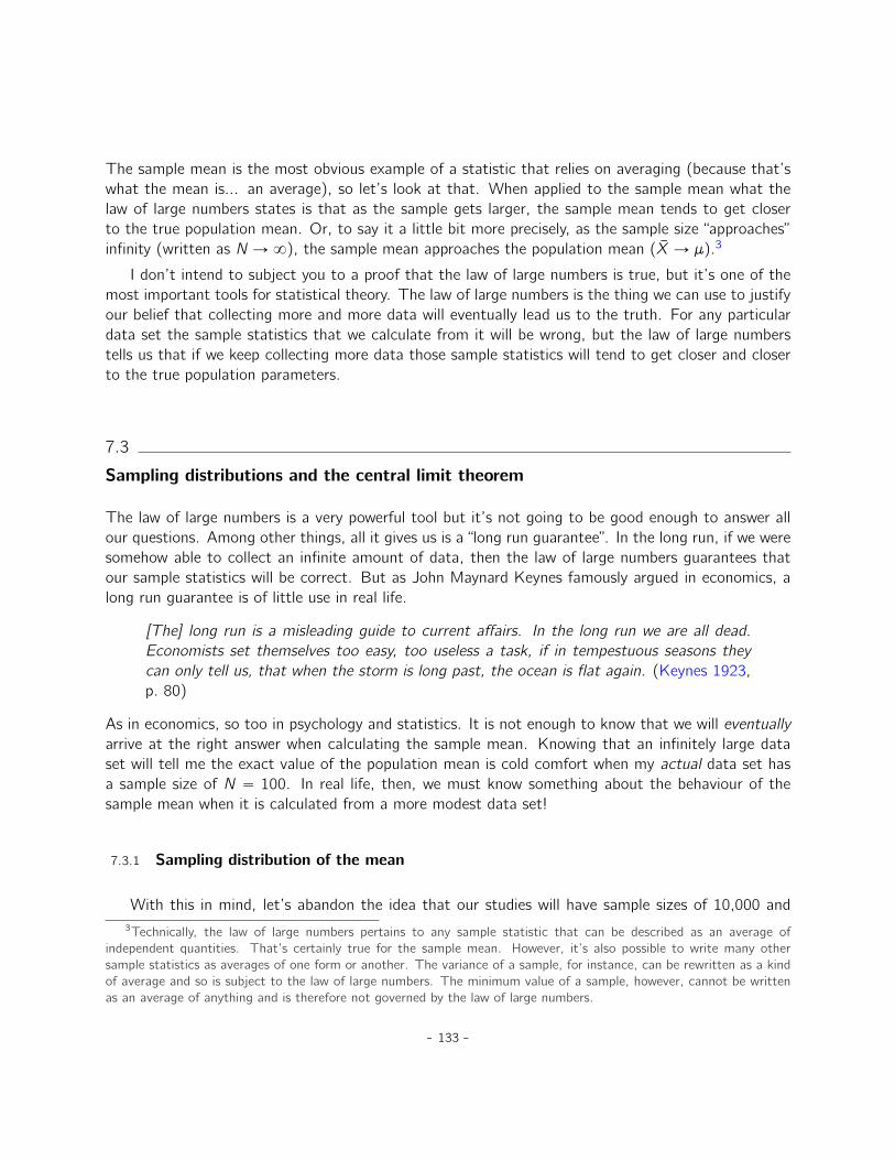
The sample mean is the most obvious example of a statistic that relies on averaging (because that’swhat the mean is... an average), so let’s look at that. When applied to the sample mean what thelaw of large numbers states is that as the sample gets larger, the sample mean tends to get closerto the true population mean. Or, to say it a little bit more precisely, as the sample size “approaches”infinity (written as N Ñ8), the sample mean approaches the population mean (X Ñ µ).3

I don’t intend to subject you to a proof that the law of large numbers is true, but it’s one of themost important tools for statistical theory. The law of large numbers is the thing we can use to justifyour belief that collecting more and more data will eventually lead us to the truth. For any particulardata set the sample statistics that we calculate from it will be wrong, but the law of large numberstells us that if we keep collecting more data those sample statistics will tend to get closer and closerto the true population parameters.

7.3

Sampling distributions and the central limit theorem

The law of large numbers is a very powerful tool but it’s not going to be good enough to answer allour questions. Among other things, all it gives us is a “long run guarantee”. In the long run, if we weresomehow able to collect an infinite amount of data, then the law of large numbers guarantees thatour sample statistics will be correct. But as John Maynard Keynes famously argued in economics, along run guarantee is of little use in real life.

[The] long run is a misleading guide to current affairs. In the long run we are all dead.Economists set themselves too easy, too useless a task, if in tempestuous seasons theycan only tell us, that when the storm is long past, the ocean is flat again. (Keynes 1923,p. 80)

As in economics, so too in psychology and statistics. It is not enough to know that we will eventuallyarrive at the right answer when calculating the sample mean. Knowing that an infinitely large dataset will tell me the exact value of the population mean is cold comfort when my actual data set hasa sample size of N “ 100. In real life, then, we must know something about the behaviour of thesample mean when it is calculated from a more modest data set!

7.3.1 Sampling distribution of the mean

With this in mind, let’s abandon the idea that our studies will have sample sizes of 10,000 and3Technically, the law of large numbers pertains to any sample statistic that can be described as an average of

independent quantities. That’s certainly true for the sample mean. However, it’s also possible to write many othersample statistics as averages of one form or another. The variance of a sample, for instance, can be rewritten as a kindof average and so is subject to the law of large numbers. The minimum value of a sample, however, cannot be writtenas an average of anything and is therefore not governed by the law of large numbers.

- 133 -

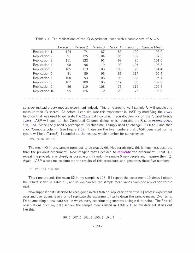
Table 7.1: Ten replications of the IQ experiment, each with a sample size of N “ 5.

Person 1 Person 2 Person 3 Person 4 Person 5 Sample MeanReplication 1 124 74 87 86 109 96.0Replication 2 91 125 104 106 109 107.0Replication 3 111 122 91 98 86 101.6Replication 4 98 96 119 99 107 103.8Replication 5 105 113 103 103 98 104.4Replication 6 81 89 93 85 114 92.4Replication 7 100 93 108 98 133 106.4Replication 8 107 100 105 117 85 102.8Replication 9 86 119 108 73 116 100.4Replication 10 95 126 112 120 76 105.8

. . . . . . . . . . . . . . . . . . . . . . . . . . . . . . . . . . . . . . . . . . . . . . . . . . . . . . . . . . . . . . . . . . . . . . . . . . . . . . . . . . . . . . . . . . . .

consider instead a very modest experiment indeed. This time around we’ll sample N “ 5 people andmeasure their IQ scores. As before, I can simulate this experiment in JASP by modifying the rnormfunction that was used to generate the IQsim data column. If you double-click on the fx label besideIQsim, JASP will open up the ‘Computed Column’ dialog, which contains the R code rnorm(10000,100, 15). Since I only need 5 participant IDs this time, I simply need to change 10000 to 5 and thenclick ‘Compute column’ (see Figure 7.6). These are the five numbers that JASP generated for me(yours will be different!). I rounded to the nearest whole number for convenience:

124 74 87 86 109

The mean IQ in this sample turns out to be exactly 96. Not surprisingly, this is much less accuratethan the previous experiment. Now imagine that I decided to replicate the experiment. That is, Irepeat the procedure as closely as possible and I randomly sample 5 new people and measure their IQ.Again, JASP allows me to simulate the results of this procedure, and generates these five numbers:

91 125 104 106 109

This time around, the mean IQ in my sample is 107. If I repeat the experiment 10 times I obtainthe results shown in Table 7.1, and as you can see the sample mean varies from one replication to thenext.

Now suppose that I decided to keep going in this fashion, replicating this “five IQ scores” experimentover and over again. Every time I replicate the experiment I write down the sample mean. Over time,I’d be amassing a new data set, in which every experiment generates a single data point. The first 10observations from my data set are the sample means listed in Table 7.1, so my data set starts outlike this:

96.0 107.0 101.6 103.8 104.4 ...

- 134 -

Figure 7.6: Using JASP to draw a random sample of 5 from a normal distribution with µ “ 100 andσ “ 15.

. . . . . . . . . . . . . . . . . . . . . . . . . . . . . . . . . . . . . . . . . . . . . . . . . . . . . . . . . . . . . . . . . . . . . . . . . . . . . . . . . . . . . . . . . . . .

- 135 -

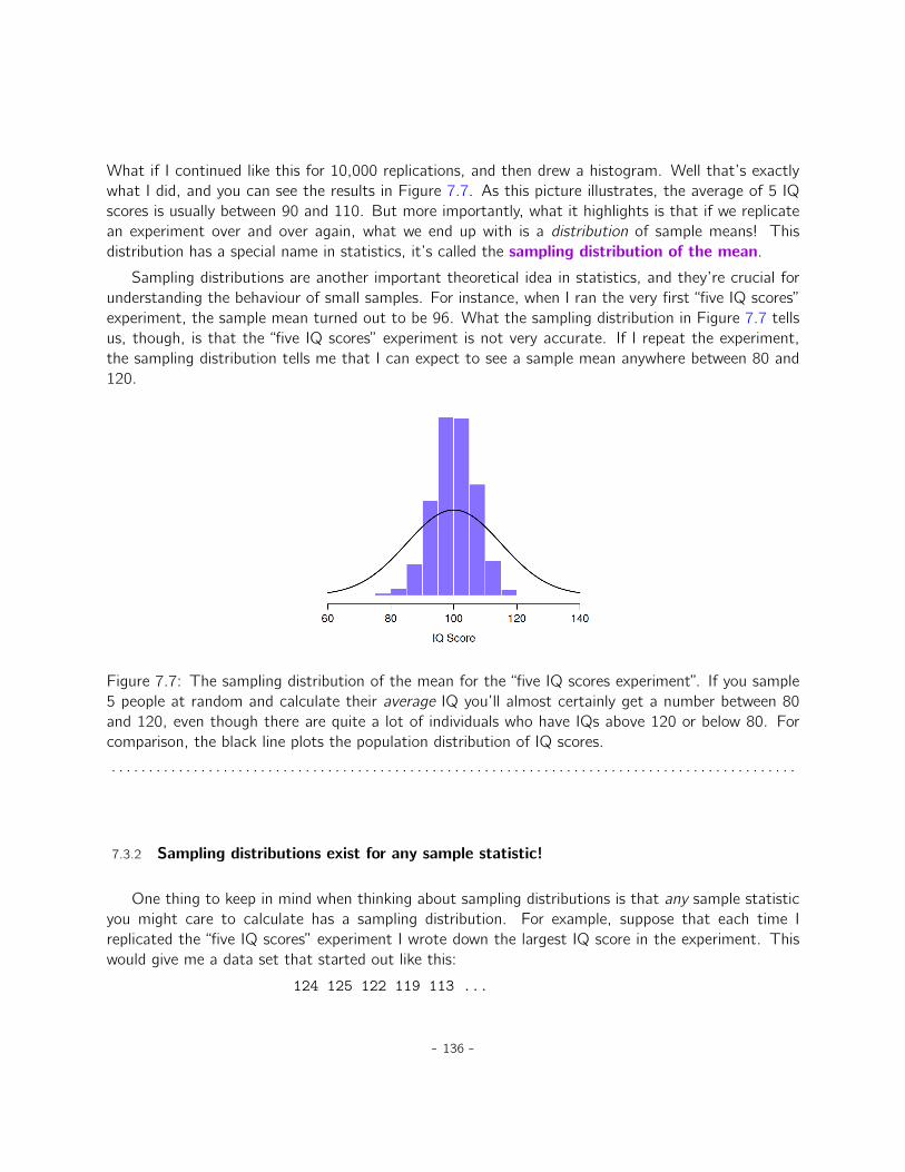
What if I continued like this for 10,000 replications, and then drew a histogram. Well that’s exactlywhat I did, and you can see the results in Figure 7.7. As this picture illustrates, the average of 5 IQscores is usually between 90 and 110. But more importantly, what it highlights is that if we replicatean experiment over and over again, what we end up with is a distribution of sample means! Thisdistribution has a special name in statistics, it’s called the sampling distribution of the mean.

Sampling distributions are another important theoretical idea in statistics, and they’re crucial forunderstanding the behaviour of small samples. For instance, when I ran the very first “five IQ scores”experiment, the sample mean turned out to be 96. What the sampling distribution in Figure 7.7 tellsus, though, is that the “five IQ scores” experiment is not very accurate. If I repeat the experiment,the sampling distribution tells me that I can expect to see a sample mean anywhere between 80 and120.

Figure 7.7: The sampling distribution of the mean for the “five IQ scores experiment”. If you sample5 people at random and calculate their average IQ you’ll almost certainly get a number between 80and 120, even though there are quite a lot of individuals who have IQs above 120 or below 80. Forcomparison, the black line plots the population distribution of IQ scores.

. . . . . . . . . . . . . . . . . . . . . . . . . . . . . . . . . . . . . . . . . . . . . . . . . . . . . . . . . . . . . . . . . . . . . . . . . . . . . . . . . . . . . . . . . . . .

7.3.2 Sampling distributions exist for any sample statistic!

One thing to keep in mind when thinking about sampling distributions is that any sample statisticyou might care to calculate has a sampling distribution. For example, suppose that each time Ireplicated the “five IQ scores” experiment I wrote down the largest IQ score in the experiment. Thiswould give me a data set that started out like this:

124 125 122 119 113 ...

- 136 -

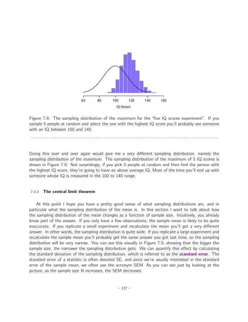
Figure 7.8: The sampling distribution of the maximum for the “five IQ scores experiment”. If yousample 5 people at random and select the one with the highest IQ score you’ll probably see someonewith an IQ between 100 and 140.

. . . . . . . . . . . . . . . . . . . . . . . . . . . . . . . . . . . . . . . . . . . . . . . . . . . . . . . . . . . . . . . . . . . . . . . . . . . . . . . . . . . . . . . . . . . .

Doing this over and over again would give me a very different sampling distribution, namely thesampling distribution of the maximum. The sampling distribution of the maximum of 5 IQ scores isshown in Figure 7.8. Not surprisingly, if you pick 5 people at random and then find the person withthe highest IQ score, they’re going to have an above average IQ. Most of the time you’ll end up withsomeone whose IQ is measured in the 100 to 140 range.

7.3.3 The central limit theorem

At this point I hope you have a pretty good sense of what sampling distributions are, and inparticular what the sampling distribution of the mean is. In this section I want to talk about howthe sampling distribution of the mean changes as a function of sample size. Intuitively, you alreadyknow part of the answer. If you only have a few observations, the sample mean is likely to be quiteinaccurate. If you replicate a small experiment and recalculate the mean you’ll get a very differentanswer. In other words, the sampling distribution is quite wide. If you replicate a large experiment andrecalculate the sample mean you’ll probably get the same answer you got last time, so the samplingdistribution will be very narrow. You can see this visually in Figure 7.9, showing that the bigger thesample size, the narrower the sampling distribution gets. We can quantify this effect by calculatingthe standard deviation of the sampling distribution, which is referred to as the standard error. Thestandard error of a statistic is often denoted SE, and since we’re usually interested in the standarderror of the sample mean, we often use the acronym SEM. As you can see just by looking at thepicture, as the sample size N increases, the SEM decreases.

- 137 -

Sample Size = 1

IQ Score

60 80 100 120 140

Sample Size = 2

IQ Score

60 80 100 120 140

Sample Size = 10

IQ Score

60 80 100 120 140

(a) (b) (c)

Figure 7.9: An illustration of the how sampling distribution of the mean depends on sample size. Ineach panel I generated 10,000 samples of IQ data and calculated the mean IQ observed within eachof these data sets. The histograms in these plots show the distribution of these means (i.e., thesampling distribution of the mean). Each individual IQ score was drawn from a normal distributionwith mean 100 and standard deviation 15, which is shown as the solid black line. In panel a, each dataset contained only a single observation, so the mean of each sample is just one person’s IQ score. As aconsequence, the sampling distribution of the mean is of course identical to the population distributionof IQ scores. However, when we raise the sample size to 2 the mean of any one sample tends to becloser to the population mean than a one person’s IQ score, and so the histogram (i.e., the samplingdistribution) is a bit narrower than the population distribution. By the time we raise the sample sizeto 10 (panel c), we can see that the distribution of sample means tend to be fairly tightly clusteredaround the true population mean.

. . . . . . . . . . . . . . . . . . . . . . . . . . . . . . . . . . . . . . . . . . . . . . . . . . . . . . . . . . . . . . . . . . . . . . . . . . . . . . . . . . . . . . . . . . . .

Okay, so that’s one part of the story. However, there’s something I’ve been glossing over so far. Allmy examples up to this point have been based on the “IQ scores” experiments, and because IQ scoresare roughly normally distributed I’ve assumed that the population distribution is normal. What if itisn’t normal? What happens to the sampling distribution of the mean? The remarkable thing is this,no matter what shape your population distribution is, as N increases the sampling distribution of themean starts to look more like a normal distribution. To give you a sense of this I ran some simulations.To do this, I started with the “ramped” distribution shown in the histogram in Figure 7.10. As youcan see by comparing the triangular shaped histogram to the bell curve plotted by the black line,the population distribution doesn’t look very much like a normal distribution at all. Next, I simulatedthe results of a large number of experiments. In each experiment I took N “ 2 samples from thisdistribution, and then calculated the sample mean. Figure 7.10b plots the histogram of these samplemeans (i.e., the sampling distribution of the mean for N “ 2). This time, the histogram produces aX-shaped distribution. It’s still not normal, but it’s a lot closer to the black line than the populationdistribution in Figure 7.10a. When I increase the sample size to N “ 4, the sampling distribution ofthe mean is very close to normal (Figure 7.10c), and by the time we reach a sample size of N “ 8 it’s

- 138 -

almost perfectly normal. In other words, as long as your sample size isn’t tiny, the sampling distributionof the mean will be approximately normal no matter what your population distribution looks like!

On the basis of these figures, it seems like we have evidence for all of the following claims aboutthe sampling distribution of the mean.

• The mean of the sampling distribution is the same as the mean of the population

• The standard deviation of the sampling distribution (i.e., the standard error) gets smaller as thesample size increases

• The shape of the sampling distribution becomes normal as the sample size increases

As it happens, not only are all of these statements true, there is a very famous theorem in statisticsthat proves all three of them, known as the central limit theorem. Among other things, the centrallimit theorem tells us that if the population distribution has mean µ and standard deviation σ, thenthe sampling distribution of the mean also has mean µ and the standard error of the mean is

SEM “σ?N

Because we divide the population standard deviation σ by the square root of the sample size N,the SEM gets smaller as the sample size increases. It also tells us that the shape of the samplingdistribution becomes normal.4

This result is useful for all sorts of things. It tells us why large experiments are more reliable thansmall ones, and because it gives us an explicit formula for the standard error it tells us how muchmore reliable a large experiment is. It tells us why the normal distribution is, well, normal. In realexperiments, many of the things that we want to measure are actually averages of lots of differentquantities (e.g., arguably, “general” intelligence as measured by IQ is an average of a large number of“specific” skills and abilities), and when that happens, the averaged quantity should follow a normaldistribution. Because of this mathematical law, the normal distribution pops up over and over againin real data.

7.4

Estimating population parameters

In all the IQ examples in the previous sections we actually knew the population parameters ahead oftime. As every undergraduate gets taught in their very first lecture on the measurement of intelligence,

4As usual, I’m being a bit sloppy here. The central limit theorem is a bit more general than this section implies. Likemost introductory stats texts I’ve discussed one situation where the central limit theorem holds: when you’re taking anaverage across lots of independent events drawn from the same distribution. However, the central limit theorem is muchbroader than this. There’s a whole class of things called “U-statistics” for instance, all of which satisfy the central limittheorem and therefore become normally distributed for large sample sizes. The mean is one such statistic, but it’s notthe only one.

- 139 -

Sample Size = 1

Sample Mean

0.0 0.2 0.4 0.6 0.8 1.0 1.2

Sample Size = 2

Sample Mean

0.0 0.2 0.4 0.6 0.8 1.0 1.2

(a) (b)

Sample Size = 4

Sample Mean

0.0 0.2 0.4 0.6 0.8 1.0 1.2

Sample Size = 8

Sample Mean

0.0 0.2 0.4 0.6 0.8 1.0 1.2

(c) (d)

Figure 7.10: A demonstration of the central limit theorem. In panel a, we have a non-normal populationdistribution, and panels b-d show the sampling distribution of the mean for samples of size 2,4 and 8for data drawn from the distribution in panel a. As you can see, even though the original populationdistribution is non-normal the sampling distribution of the mean becomes pretty close to normal bythe time you have a sample of even 4 observations.

. . . . . . . . . . . . . . . . . . . . . . . . . . . . . . . . . . . . . . . . . . . . . . . . . . . . . . . . . . . . . . . . . . . . . . . . . . . . . . . . . . . . . . . . . . . .

- 140 -

IQ scores are defined to have mean 100 and standard deviation 15. However, this is a bit of a lie.How do we know that IQ scores have a true population mean of 100? Well, we know this becausethe people who designed the tests have administered them to very large samples, and have then“rigged” the scoring rules so that their sample has mean 100. That’s not a bad thing of course, it’san important part of designing a psychological measurement. However, it’s important to keep in mindthat this theoretical mean of 100 only attaches to the population that the test designers used todesign the tests. Good test designers will actually go to some lengths to provide “test norms” thatcan apply to lots of different populations (e.g., different age groups, nationalities etc).

This is very handy, but of course almost every research project of interest involves looking at adifferent population of people to those used in the test norms. For instance, suppose you wanted tomeasure the effect of low level lead poisoning on cognitive functioning in Port Pirie, a South Australianindustrial town with a lead smelter. Perhaps you decide that you want to compare IQ scores amongpeople in Port Pirie to a comparable sample in Whyalla, a South Australian industrial town with asteel refinery.5 Regardless of which town you’re thinking about, it doesn’t make a lot of sense simplyto assume that the true population mean IQ is 100. No-one has, to my knowledge, produced sensiblenorming data that can automatically be applied to South Australian industrial towns. We’re going tohave to estimate the population parameters from a sample of data. So how do we do this?

7.4.1 Estimating the population mean

Suppose we go to Port Pirie and 100 of the locals are kind enough to sit through an IQ test.The average IQ score among these people turns out to be X “ 98.5. So what is the true mean IQfor the entire population of Port Pirie? Obviously, we don’t know the answer to that question. Itcould be 97.2, but it could also be 103.5. Our sampling isn’t exhaustive so we cannot give a definitiveanswer. Nevertheless, if I was forced at gunpoint to give a “best guess” I’d have to say 98.5. That’sthe essence of statistical estimation: giving a best guess.

In this example estimating the unknown poulation parameter is straightforward. I calculate thesample mean and I use that as my estimate of the population mean. It’s pretty simple, and inthe next section I’ll explain the statistical justification for this intuitive answer. However, for the

5Please note that if you were actually interested in this question you would need to be a lot more careful than I’mbeing here. You can’t just compare IQ scores in Whyalla to Port Pirie and assume that any differences are due to leadpoisoning. Even if it were true that the only differences between the two towns corresponded to the different refineries(and it isn’t, not by a long shot), you need to account for the fact that people already believe that lead pollution causescognitive deficits. If you recall back to Chapter 2, this means that there are different demand effects for the Port Piriesample than for the Whyalla sample. In other words, you might end up with an illusory group difference in your data,caused by the fact that people think that there is a real difference. I find it pretty implausible to think that the localswouldn’t be well aware of what you were trying to do if a bunch of researchers turned up in Port Pirie with lab coats andIQ tests, and even less plausible to think that a lot of people would be pretty resentful of you for doing it. Those peoplewon’t be as co-operative in the tests. Other people in Port Pirie might be more motivated to do well because they don’twant their home town to look bad. The motivational effects that would apply in Whyalla are likely to be weaker, becausepeople don’t have any concept of “iron ore poisoning” in the same way that they have a concept for “lead poisoning”.Psychology is hard.

- 141 -

moment what I want to do is make sure you recognise that the sample statistic and the estimate ofthe population parameter are conceptually different things. A sample statistic is a description of yourdata, whereas the estimate is a guess about the population. With that in mind, statisticians oftendifferent notation to refer to them. For instance, if the true population mean is denoted µ, thenwe would use µ to refer to our estimate of the population mean. In contrast, the sample mean isdenoted X or sometimes m. However, in simple random samples the estimate of the population meanis identical to the sample mean. If I observe a sample mean of X “ 98.5 then my estimate of thepopulation mean is also µ “ 98.5. To help keep the notation clear, here’s a handy table:

Symbol What is it? Do we know what it is?

X Sample mean Yes, calculated from the raw dataµ True population mean Almost never known for sureµ Estimate of the population mean Yes, identical to the sample mean in sim-

ple random samples

7.4.2 Estimating the population standard deviation

So far, estimation seems pretty simple, and you might be wondering why I forced you to readthrough all that stuff about sampling theory. In the case of the mean our estimate of the populationparameter (i.e. µ) turned out to identical to the corresponding sample statistic (i.e. X). However,that’s not always true. To see this, let’s have a think about how to construct an estimate of thepopulation standard deviation, which we’ll denote σ. What shall we use as our estimate in this case?Your first thought might be that we could do the same thing we did when estimating the mean, andjust use the sample statistic as our estimate. That’s almost the right thing to do, but not quite.

Here’s why. Suppose I have a sample that contains a single observation. For this example, it helpsto consider a sample where you have no intuitions at all about what the true population values mightbe, so let’s use something completely fictitious. Suppose the observation in question measures thecromulence of my shoes. It turns out that my shoes have a cromulence of 20. So here’s my sample:

20

This is a perfectly legitimate sample, even if it does have a sample size of N “ 1. It has a samplemean of 20 and because every observation in this sample is equal to the sample mean (obviously!)it has a sample standard deviation of 0. As a description of the sample this seems quite right, thesample contains a single observation and therefore there is no variation observed within the sample.A sample standard deviation of s “ 0 is the right answer here. But as an estimate of the populationstandard deviation it feels completely insane, right? Admittedly, you and I don’t know anything at allabout what “cromulence” is, but we know something about data. The only reason that we don’t seeany variability in the sample is that the sample is too small to display any variation! So, if you have asample size of N “ 1 it feels like the right answer is just to say “no idea at all”.

Notice that you don’t have the same intuition when it comes to the sample mean and the population

- 142 -

mean. If forced to make a best guess about the population mean it doesn’t feel completely insane toguess that the population mean is 20. Sure, you probably wouldn’t feel very confident in that guessbecause you have only the one observation to work with, but it’s still the best guess you can make.

Let’s extend this example a little. Suppose I now make a second observation. My data set nowhas N “ 2 observations of the cromulence of shoes, and the complete sample now looks like this:

20, 22

This time around, our sample is just large enough for us to be able to observe some variability: twoobservations is the bare minimum number needed for any variability to be observed! For our new dataset, the sample mean is X “ 21, and the sample standard deviation is s “ 1. What intuitions dowe have about the population? Again, as far as the population mean goes, the best guess we canpossibly make is the sample mean. If forced to guess we’d probably guess that the population meancromulence is 21. What about the standard deviation? This is a little more complicated. The samplestandard deviation is only based on two observations, and if you’re at all like me you probably havethe intuition that, with only two observations we haven’t given the population “enough of a chance”to reveal its true variability to us. It’s not just that we suspect that the estimate is wrong, after allwith only two observations we expect it to be wrong to some degree. The worry is that the error issystematic. Specifically, we suspect that the sample standard deviation is likely to be smaller than thepopulation standard deviation.

This intuition feels right, but it would be nice to demonstrate this somehow. There are in factmathematical proofs that confirm this intuition, but unless you have the right mathematical back-ground they don’t help very much. Instead, what I’ll do is simulate the results of some experiments.With that in mind, let’s return to our IQ studies. Suppose the true population mean IQ is 100 andthe standard deviation is 15. First I’ll conduct an experiment in which I measure N “ 2 IQ scores andI’ll calculate the sample standard deviation. If I do this over and over again, and plot a histogram ofthese sample standard deviations, what I have is the sampling distribution of the standard deviation.I’ve plotted this distribution in Figure 7.11. Even though the true population standard deviation is 15the average of the sample standard deviations is only 8.5. Notice that this is a very different resultto what we found in Figure 7.9b when we plotted the sampling distribution of the mean, where thepopulation mean is 100 and the average of the sample means is also 100.

Now let’s extend the simulation. Instead of restricting ourselves to the situation where N “ 2, let’srepeat the exercise for sample sizes from 1 to 10. If we plot the average sample mean and averagesample standard deviation as a function of sample size, you get the results shown in Figure 7.12. Onthe left hand side (panel a) I’ve plotted the average sample mean and on the right hand side (panel b)I’ve plotted the average standard deviation. The two plots are quite different:on average, the averagesample mean is equal to the population mean. It is an unbiased estimator, which is essentially thereason why your best estimate for the population mean is the sample mean.6 The plot on the right is

6I should note that I’m hiding something here. Unbiasedness is a desirable characteristic for an estimator, but thereare other things that matter besides bias. However, it’s beyond the scope of this book to discuss this in any detail. I justwant to draw your attention to the fact that there’s some hidden complexity here.

- 143 -

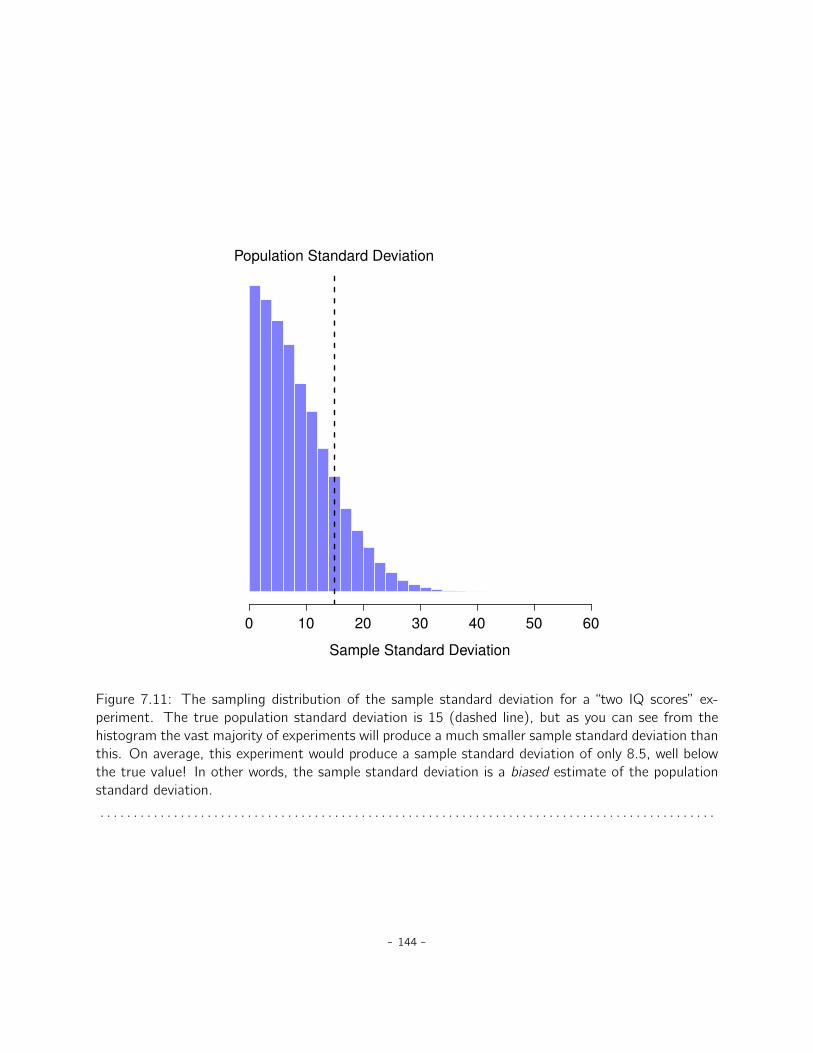
Sample Standard Deviation

0 10 20 30 40 50 60

Population Standard Deviation

Figure 7.11: The sampling distribution of the sample standard deviation for a “two IQ scores” ex-periment. The true population standard deviation is 15 (dashed line), but as you can see from thehistogram the vast majority of experiments will produce a much smaller sample standard deviation thanthis. On average, this experiment would produce a sample standard deviation of only 8.5, well belowthe true value! In other words, the sample standard deviation is a biased estimate of the populationstandard deviation.

. . . . . . . . . . . . . . . . . . . . . . . . . . . . . . . . . . . . . . . . . . . . . . . . . . . . . . . . . . . . . . . . . . . . . . . . . . . . . . . . . . . . . . . . . . . .

- 144 -

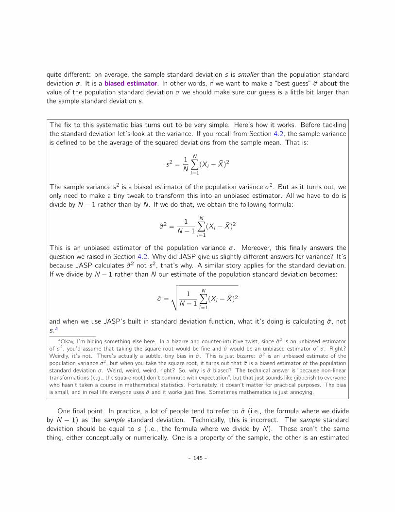
quite different: on average, the sample standard deviation s is smaller than the population standarddeviation σ. It is a biased estimator. In other words, if we want to make a “best guess” σ about thevalue of the population standard deviation σ we should make sure our guess is a little bit larger thanthe sample standard deviation s.

The fix to this systematic bias turns out to be very simple. Here’s how it works. Before tacklingthe standard deviation let’s look at the variance. If you recall from Section 4.2, the sample varianceis defined to be the average of the squared deviations from the sample mean. That is:

s2 “1

N

Nÿ

i“1

pXi ´ Xq2

The sample variance s2 is a biased estimator of the population variance σ2. But as it turns out, weonly need to make a tiny tweak to transform this into an unbiased estimator. All we have to do isdivide by N ´ 1 rather than by N. If we do that, we obtain the following formula:

σ2 “1

N ´ 1

Nÿ

i“1

pXi ´ Xq2

This is an unbiased estimator of the population variance σ. Moreover, this finally answers thequestion we raised in Section 4.2. Why did JASP give us slightly different answers for variance? It’sbecause JASP calculates σ2 not s2, that’s why. A similar story applies for the standard deviation.If we divide by N ´ 1 rather than N our estimate of the population standard deviation becomes:

σ “

g

f

f

e

1

N ´ 1

Nÿ

i“1

pXi ´ Xq2

and when we use JASP’s built in standard deviation function, what it’s doing is calculating σ, nots.a

aOkay, I’m hiding something else here. In a bizarre and counter-intuitive twist, since σ2 is an unbiased estimatorof σ2, you’d assume that taking the square root would be fine and σ would be an unbiased estimator of σ. Right?Weirdly, it’s not. There’s actually a subtle, tiny bias in σ. This is just bizarre: σ2 is an unbiased estimate of thepopulation variance σ2, but when you take the square root, it turns out that σ is a biased estimator of the populationstandard deviation σ. Weird, weird, weird, right? So, why is σ biased? The technical answer is “because non-lineartransformations (e.g., the square root) don’t commute with expectation”, but that just sounds like gibberish to everyonewho hasn’t taken a course in mathematical statistics. Fortunately, it doesn’t matter for practical purposes. The biasis small, and in real life everyone uses σ and it works just fine. Sometimes mathematics is just annoying.

One final point. In practice, a lot of people tend to refer to σ (i.e., the formula where we divideby N ´ 1) as the sample standard deviation. Technically, this is incorrect. The sample standarddeviation should be equal to s (i.e., the formula where we divide by N). These aren’t the samething, either conceptually or numerically. One is a property of the sample, the other is an estimated

- 145 -

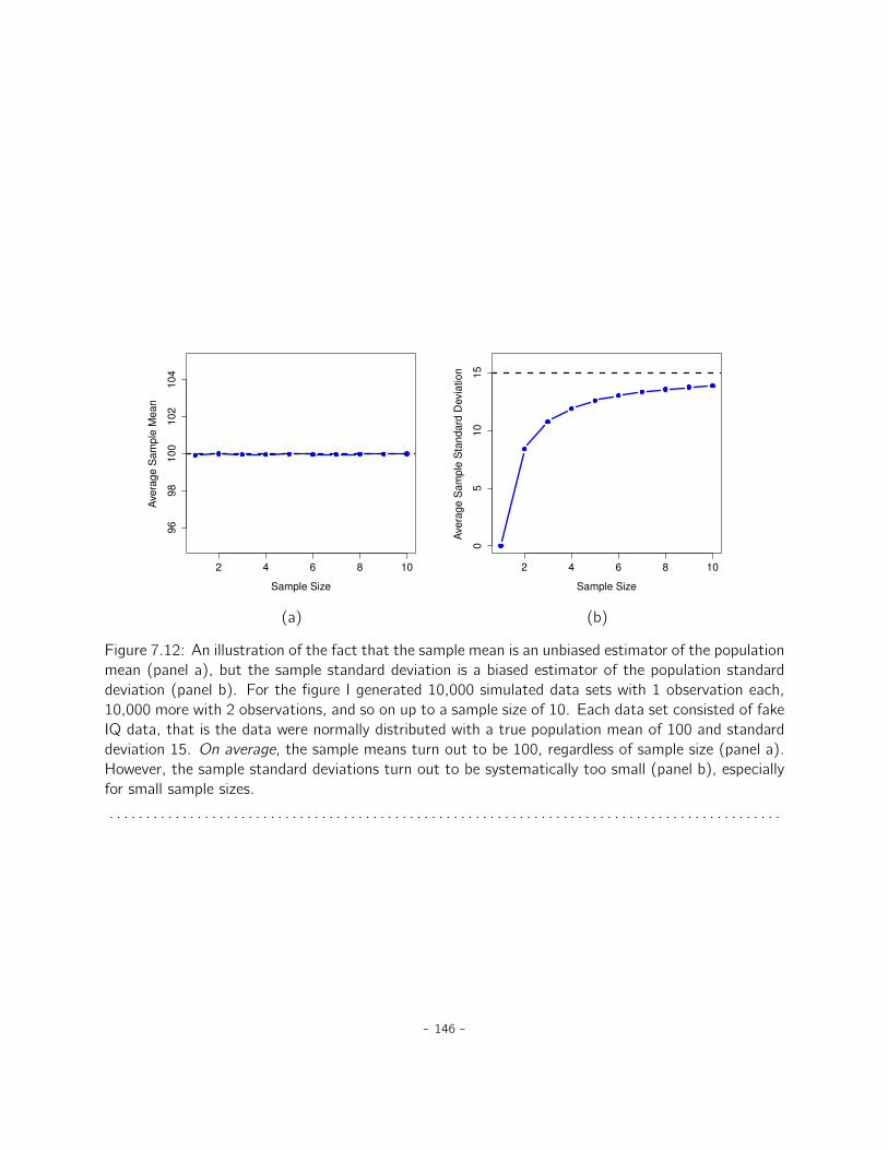
2 4 6 8 10

96

98

10

01

02

10

4

Sample Size

Ave

rag

e S

am

ple

Me

an

2 4 6 8 10

05

10

15

Sample Size

Ave

rag

e S

am

ple

Sta

nd

ard

Devia

tio

n

(a) (b)

Figure 7.12: An illustration of the fact that the sample mean is an unbiased estimator of the populationmean (panel a), but the sample standard deviation is a biased estimator of the population standarddeviation (panel b). For the figure I generated 10,000 simulated data sets with 1 observation each,10,000 more with 2 observations, and so on up to a sample size of 10. Each data set consisted of fakeIQ data, that is the data were normally distributed with a true population mean of 100 and standarddeviation 15. On average, the sample means turn out to be 100, regardless of sample size (panel a).However, the sample standard deviations turn out to be systematically too small (panel b), especiallyfor small sample sizes.

. . . . . . . . . . . . . . . . . . . . . . . . . . . . . . . . . . . . . . . . . . . . . . . . . . . . . . . . . . . . . . . . . . . . . . . . . . . . . . . . . . . . . . . . . . . .

- 146 -

characteristic of the population. However, in almost every real life application what we actually careabout is the estimate of the population parameter, and so people always report σ rather than s. Thisis the right number to report, of course. It’s just that people tend to get a little bit imprecise aboutterminology when they write it up, because “sample standard deviation” is shorter than “estimatedpopulation standard deviation”. It’s no big deal, and in practice I do the same thing everyone elsedoes. Nevertheless, I think it’s important to keep the two concepts separate. It’s never a good idea toconfuse “known properties of your sample” with “guesses about the population from which it came”.The moment you start thinking that s and σ are the same thing, you start doing exactly that.

To finish this section off, here’s another couple of tables to help keep things clear.


s Sample standard deviation Yes, calculated from the raw dataσ Population standard deviation Almost never known for sureσ Estimate of the population Yes, but not the same as the

standard deviation sample standard deviation


s2 Sample variance Yes, calculated from the raw dataσ2 Population variance Almost never known for sureσ2 Estimate of the population Yes, but not the same as the

variance sample variance

7.5

Estimating a confidence interval

Statistics means never having to say you’re certain

– Unknown origin7

Up to this point in this chapter, I’ve outlined the basics of sampling theory which statisticians rely onto make guesses about population parameters on the basis of a sample of data. As this discussionillustrates, one of the reasons we need all this sampling theory is that every data set leaves us with asome of uncertainty, so our estimates are never going to be perfectly accurate. The thing that hasbeen missing from this discussion is an attempt to quantify the amount of uncertainty that attaches

7This quote appears on a great many t-shirts and websites, and even gets a mention in a few academic papers (e.g.,http://www.amstat.org/publications/jse/v10n3/friedman.html, but I’ve never found the original source.

- 147 -

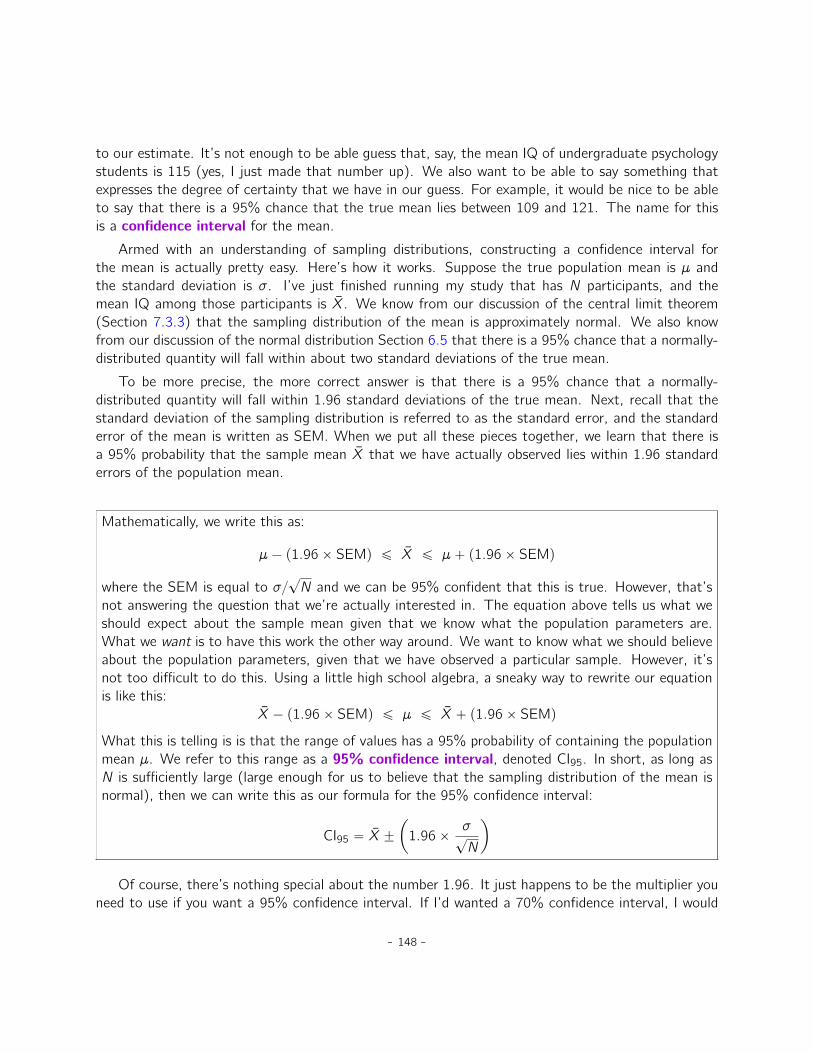
http://www.amstat.org/publications/jse/v10n3/friedman.html

to our estimate. It’s not enough to be able guess that, say, the mean IQ of undergraduate psychologystudents is 115 (yes, I just made that number up). We also want to be able to say something thatexpresses the degree of certainty that we have in our guess. For example, it would be nice to be ableto say that there is a 95% chance that the true mean lies between 109 and 121. The name for thisis a confidence interval for the mean.

Armed with an understanding of sampling distributions, constructing a confidence interval forthe mean is actually pretty easy. Here’s how it works. Suppose the true population mean is µ andthe standard deviation is σ. I’ve just finished running my study that has N participants, and themean IQ among those participants is X. We know from our discussion of the central limit theorem(Section 7.3.3) that the sampling distribution of the mean is approximately normal. We also knowfrom our discussion of the normal distribution Section 6.5 that there is a 95% chance that a normally-distributed quantity will fall within about two standard deviations of the true mean.

To be more precise, the more correct answer is that there is a 95% chance that a normally-distributed quantity will fall within 1.96 standard deviations of the true mean. Next, recall that thestandard deviation of the sampling distribution is referred to as the standard error, and the standarderror of the mean is written as SEM. When we put all these pieces together, we learn that there isa 95% probability that the sample mean X that we have actually observed lies within 1.96 standarderrors of the population mean.

Mathematically, we write this as:

µ´ p1.96ˆ SEMq ď X ď µ` p1.96ˆ SEMq

where the SEM is equal to σ{?N and we can be 95% confident that this is true. However, that’s

not answering the question that we’re actually interested in. The equation above tells us what weshould expect about the sample mean given that we know what the population parameters are.What we want is to have this work the other way around. We want to know what we should believeabout the population parameters, given that we have observed a particular sample. However, it’snot too difficult to do this. Using a little high school algebra, a sneaky way to rewrite our equationis like this:

X ´ p1.96ˆ SEMq ď µ ď X ` p1.96ˆ SEMq

What this is telling is is that the range of values has a 95% probability of containing the populationmean µ. We refer to this range as a 95% confidence interval, denoted CI95. In short, as long asN is sufficiently large (large enough for us to believe that the sampling distribution of the mean isnormal), then we can write this as our formula for the 95% confidence interval:

CI95 “ X ˘

ˆ

1.96ˆσ?N

˙

Of course, there’s nothing special about the number 1.96. It just happens to be the multiplier youneed to use if you want a 95% confidence interval. If I’d wanted a 70% confidence interval, I would

- 148 -

have used 1.04 as the magic number rather than 1.96.

7.5.1 A slight mistake in the formula

As usual, I lied. The formula that I’ve given above for the 95% confidence interval is approximatelycorrect, but I glossed over an important detail in the discussion. Notice my formula requires you to usethe standard error of the mean, SEM, which in turn requires you to use the true population standarddeviation σ. Yet, in Section 7.4 I stressed the fact that we don’t actually know the true populationparameters. Because we don’t know the true value of σ we have to use an estimate of the populationstandard deviation σ instead. This is pretty straightforward to do, but this has the consequence thatwe need to use the percentiles of the t-distribution rather than the normal distribution to calculateour magic number, and the answer depends on the sample size. When N is very large, we get prettymuch the same value using the t-distribution or the normal distribution: 1.96. But when N is smallwe get a much bigger number when we use the t distribution: 2.26.

There’s nothing too mysterious about what’s happening here. Bigger values mean that the confi-dence interval is wider, indicating that we’re more uncertain about what the true value of µ actuallyis. When we use the t distribution instead of the normal distribution we get bigger numbers, indicat-ing that we have more uncertainty. And why do we have that extra uncertainty? Well, because ourestimate of the population standard deviation σ might be wrong! If it’s wrong, it implies that we’re abit less sure about what our sampling distribution of the mean actually looks like, and this uncertaintyends up getting reflected in a wider confidence interval.

7.5.2 Interpreting a confidence interval

The hardest thing about confidence intervals is understanding what they mean. Whenever peoplefirst encounter confidence intervals, the first instinct is almost always to say that “there is a 95%probability that the true mean lies inside the confidence interval”. It’s simple and it seems to capturethe common sense idea of what it means to say that I am “95% confident”. Unfortunately, it’s notquite right. The intuitive definition relies very heavily on your own personal beliefs about the valueof the population mean. I say that I am 95% confident because those are my beliefs. In everydaylife that’s perfectly okay, but if you remember back to Section 6.2, you’ll notice that talking aboutpersonal belief and confidence is a Bayesian idea. However, confidence intervals are not Bayesian tools.Like everything else in this chapter, confidence intervals are frequentist tools, and if you are going touse frequentist methods then it’s not appropriate to attach a Bayesian interpretation to them. If youuse frequentist methods, you must adopt frequentist interpretations!

Okay, so if that’s not the right answer, what is? Remember what we said about frequentistprobability. The only way we are allowed to make “probability statements” is to talk about a sequenceof events, and to count up the frequencies of different kinds of events. From that perspective, theinterpretation of a 95% confidence interval must have something to do with replication. Specifically,if we replicated the experiment over and over again and computed a 95% confidence interval for each

- 149 -

replication, then 95% of those intervals would contain the true mean. More generally, 95% of allconfidence intervals constructed using this procedure should contain the true population mean. Thisidea is illustrated in Figure 7.13, which shows 50 confidence intervals constructed for a “measure 10IQ scores” experiment (top panel) and another 50 confidence intervals for a “measure 25 IQ scores”experiment (bottom panel). A bit fortuitously, across the 100 replications that I simulated, it turnedout that exactly 95 of them contained the true mean.

The critical difference here is that the Bayesian claim makes a probability statement about thepopulation mean (i.e., it refers to our uncertainty about the population mean), which is not allowedunder the frequentist interpretation of probability because you can’t “replicate” a population! Inthe frequentist claim, the population mean is fixed and no probabilistic claims can be made about it.Confidence intervals, however, are repeatable so we can replicate experiments. Therefore a frequentistis allowed to talk about the probability that the confidence interval (a random variable) contains thetrue mean, but is not allowed to talk about the probability that the true population mean (not arepeatable event) falls within the confidence interval.

I know that this seems a little pedantic, but it does matter. It matters because the difference ininterpretation leads to a difference in the mathematics. There is a Bayesian alternative to confidenceintervals, known as credible intervals. In most situations credible intervals are quite similar to confi-dence intervals, but in other cases they are drastically different. As promised, though, I’ll talk moreabout the Bayesian perspective in Chapter 14.

7.5.3 Calculating confidence intervals in JASP

As of this edition, JASP does not (yet) include a simple way to calculate confidence intervals forthe mean as part of the ‘Descriptives’ functionality. But the ‘Descriptives’ do have a check box forthe S.E. Mean, so you can use this to calculate the lower 95% confidence interval as:

Mean - (1.96 * S.E. Mean) , and the upper 95% confidence interval as:

Mean + (1.96 * S.E. Mean)

95% confidence intervals are the de facto standard in psychology. So, for example, if I load theIQsim.jasp file, check mean and S.E mean under ‘Descriptives’, I can work out the confidence intervalassociated with the simulated mean IQ:

Lower 95% CI = 100.107 - (1.96 * 0.150) = 99.813

Upper 95% CI = 100.107 + (1.96 * 0.150) = 100.401

So, in our simulated large sample data with N=10,000, the mean IQ score is 100.107 with a 95%CI from 99.813 to 100.401. Hopefully that’s clear and fairly easy to interpret. So, although therecurrently is not a straightforward way to get JASP to calculate the confidence interval as part of thevariable ‘Descriptives’ options, if we wanted to we could pretty easily work it out by hand.

Similarly, when it comes to plotting confidence intervals in JASP, this is also not (yet) availableas part of the ‘Descriptives’ options. However, when we get onto learning about specific statisticaltests, for example in Chapter 12, we will see that we can plot confidence intervals as part of the data

- 150 -

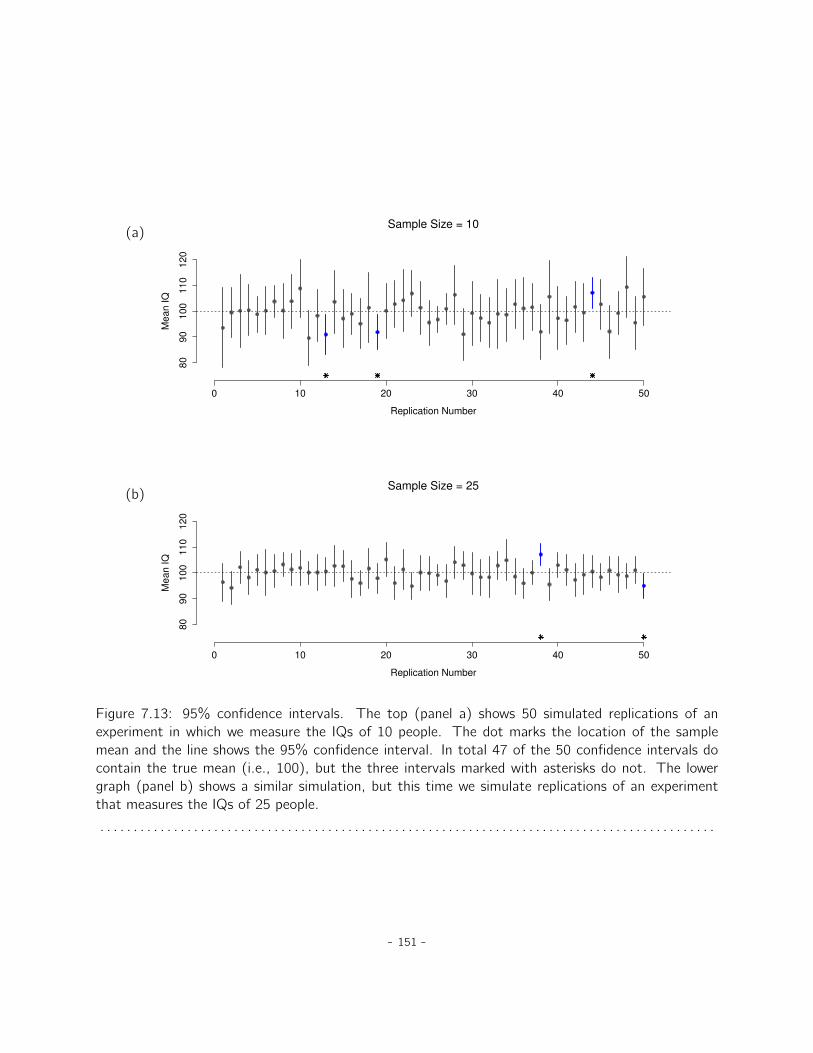
(a)

0 10 20 30 40 50

80

90

10

01

10

12

0

Sample Size = 10

Replication Number

Me

an

IQ

(b)

0 10 20 30 40 50

80

90

10

01

10

12

0

Sample Size = 25

Replication Number

Me

an

IQ

Figure 7.13: 95% confidence intervals. The top (panel a) shows 50 simulated replications of anexperiment in which we measure the IQs of 10 people. The dot marks the location of the samplemean and the line shows the 95% confidence interval. In total 47 of the 50 confidence intervals docontain the true mean (i.e., 100), but the three intervals marked with asterisks do not. The lowergraph (panel b) shows a similar simulation, but this time we simulate replications of an experimentthat measures the IQs of 25 people.

. . . . . . . . . . . . . . . . . . . . . . . . . . . . . . . . . . . . . . . . . . . . . . . . . . . . . . . . . . . . . . . . . . . . . . . . . . . . . . . . . . . . . . . . . . . .

- 151 -

analysis. That’s pretty cool, so we’ll show you how to do that later on.

7.6

Summary

In this chapter I’ve covered two main topics. The first half of the chapter talks about samplingtheory, and the second half talks about how we can use sampling theory to construct estimates of thepopulation parameters. The section breakdown looks like this:

• Basic ideas about samples, sampling and populations (Section 7.1)

• Statistical theory of sampling: the law of large numbers (Section 7.2), sampling distributionsand the central limit theorem (Section 7.3).

• Estimating means and standard deviations (Section 7.4)

• Estimating a confidence interval (Section 7.5)

As always, there’s a lot of topics related to sampling and estimation that aren’t covered in thischapter, but for an introductory psychology class this is fairly comprehensive I think. For most appliedresearchers you won’t need much more theory than this. One big question that I haven’t touchedon in this chapter is what you do when you don’t have a simple random sample. There is a lot ofstatistical theory you can draw on to handle this situation, but it’s well beyond the scope of this book.

- 152 -

8. Hypothesis testing

The process of induction is the process of assuming the simplest law that can be made toharmonize with our experience. This process, however, has no logical foundation but onlya psychological one. It is clear that there are no grounds for believing that the simplestcourse of events will really happen. It is an hypothesis that the sun will rise tomorrow:and this means that we do not know whether it will rise.

– Ludwig Wittgenstein1

In the last chapter I discussed the ideas behind estimation, which is one of the two “big ideas” ininferential statistics. It’s now time to turn our attention to the other big idea, which is hypothesistesting. In its most abstract form, hypothesis testing is really a very simple idea. The researcher hassome theory about the world and wants to determine whether or not the data actually support thattheory. However, the details are messy and most people find the theory of hypothesis testing to bethe most frustrating part of statistics. The structure of the chapter is as follows. First, I’ll describehow hypothesis testing works in a fair amount of detail, using a simple running example to show youhow a hypothesis test is “built”. I’ll try to avoid being too dogmatic while doing so, and focus insteadon the underlying logic of the testing procedure.2 Afterwards, I’ll spend a bit of time talking aboutthe various dogmas, rules and heresies that surround the theory of hypothesis testing.

1The quote comes from Wittgenstein’s (1922) text, Tractatus Logico-Philosphicus.2A technical note. The description below differs subtly from the standard description given in a lot of introductory

texts. The orthodox theory of null hypothesis testing emerged from the work of Sir Ronald Fisher and Jerzy Neyman inthe early 20th century; but Fisher and Neyman actually had very different views about how it should work. The standardtreatment of hypothesis testing that most texts use is a hybrid of the two approaches. The treatment here is a littlemore Neyman-style than the orthodox view, especially as regards the meaning of the p value.

- 153 -

8.1

A menagerie of hypotheses

Eventually we all succumb to madness. For me, that day will arrive once I’m finally promoted tofull professor. Safely ensconced in my ivory tower, happily protected by tenure, I will finally be ableto take leave of my senses (so to speak) and indulge in that most thoroughly unproductive line ofpsychological research, the search for extrasensory perception (ESP).3

Let’s suppose that this glorious day has come. My first study is a simple one in which I seek totest whether clairvoyance exists. Each participant sits down at a table and is shown a card by anexperimenter. The card is black on one side and white on the other. The experimenter takes the cardaway and places it on a table in an adjacent room. The card is placed black side up or white side upcompletely at random, with the randomisation occurring only after the experimenter has left the roomwith the participant. A second experimenter comes in and asks the participant which side of the cardis now facing upwards. It’s purely a one-shot experiment. Each person sees only one card and givesonly one answer, and at no stage is the participant actually in contact with someone who knows theright answer. My data set, therefore, is very simple. I have asked the question of N people and somenumber X of these people have given the correct response. To make things concrete, let’s supposethat I have tested N “ 100 people and X “ 62 of these got the answer right. A surprisingly largenumber, sure, but is it large enough for me to feel safe in claiming I’ve found evidence for ESP? Thisis the situation where hypothesis testing comes in useful. However, before we talk about how to testhypotheses, we need to be clear about what we mean by hypotheses.

8.1.1 Research hypotheses versus statistical hypotheses

The first distinction that you need to keep clear in your mind is between research hypotheses andstatistical hypotheses. In my ESP study my overall scientific goal is to demonstrate that clairvoyanceexists. In this situation I have a clear research goal: I am hoping to discover evidence for ESP. Inother situations I might actually be a lot more neutral than that, so I might say that my research goalis to determine whether or not clairvoyance exists. Regardless of how I want to portray myself, thebasic point that I’m trying to convey here is that a research hypothesis involves making a substantive,testable scientific claim. If you are a psychologist then your research hypotheses are fundamentallyabout psychological constructs. Any of the following would count as research hypotheses:

• Listening to music reduces your ability to pay attention to other things. This is a claim aboutthe causal relationship between two psychologically meaningful concepts (listening to music andpaying attention to things), so it’s a perfectly reasonable research hypothesis.

3My apologies to anyone who actually believes in this stuff, but on my reading of the literature on ESP it’s justnot reasonable to think this is real. To be fair, though, some of the studies are rigorously designed, so it’s actually aninteresting area for thinking about psychological research design. And of course it’s a free country so you can spend yourown time and effort proving me wrong if you like, but I wouldn’t think that’s a terribly practical use of your intellect.

- 154 -

• Intelligence is related to personality. Like the last one, this is a relational claim about twopsychological constructs (intelligence and personality), but the claim is weaker: correlationalnot causal.

• Intelligence is speed of information processing. This hypothesis has a quite different character.It’s not actually a relational claim at all. It’s an ontological claim about the fundamental characterof intelligence (and I’m pretty sure it’s wrong). It’s worth expanding on this one actually. It’susually easier to think about how to construct experiments to test research hypotheses of theform “does X affect Y?” than it is to address claims like “what is X?” And in practice what usuallyhappens is that you find ways of testing relational claims that follow from your ontological ones.For instance, if I believe that intelligence is speed of information processing in the brain, myexperiments will often involve looking for relationships between measures of intelligence andmeasures of speed. As a consequence most everyday research questions do tend to be relationalin nature, but they’re almost always motivated by deeper ontological questions about the stateof nature.

Notice that in practice, my research hypotheses could overlap a lot. My ultimate goal in the ESPexperiment might be to test an ontological claim like “ESP exists”, but I might operationally restrictmyself to a narrower hypothesis like “Some people can ‘see’ objects in a clairvoyant fashion”. Thatsaid, there are some things that really don’t count as proper research hypotheses in any meaningfulsense:

• Love is a battlefield. This is too vague to be testable. Whilst it’s okay for a research hypothesisto have a degree of vagueness to it, it has to be possible to operationalise your theoretical ideas.Maybe I’m just not creative enough to see it, but I can’t see how this can be converted intoany concrete research design. If that’s true then this isn’t a scientific research hypothesis, it’sa pop song. That doesn’t mean it’s not interesting. A lot of deep questions that humans havefall into this category. Maybe one day science will be able to construct testable theories of love,or to test to see if God exists, and so on. But right now we can’t, and I wouldn’t bet on everseeing a satisfying scientific approach to either.

• The first rule of tautology club is the first rule of tautology club. This is not a substantive claimof any kind. It’s true by definition. No conceivable state of nature could possibly be inconsistentwith this claim. We say that this is an unfalsifiable hypothesis, and as such it is outside thedomain of science. Whatever else you do in science your claims must have the possibility ofbeing wrong.

• More people in my experiment will say “yes” than “no” . This one fails as a research hypothesisbecause it’s a claim about the data set, not about the psychology (unless of course your actualresearch question is whether people have some kind of “yes” bias!). Actually, this hypothesis isstarting to sound more like a statistical hypothesis than a research hypothesis.

As you can see, research hypotheses can be somewhat messy at times and ultimately they arescientific claims. Statistical hypotheses are neither of these two things. Statistical hypotheses must

- 155 -

be mathematically precise and they must correspond to specific claims about the characteristics of thedata generating mechanism (i.e., the “population”). Even so, the intent is that statistical hypothesesbear a clear relationship to the substantive research hypotheses that you care about! For instance, inmy ESP study my research hypothesis is that some people are able to see through walls or whatever.What I want to do is to “map” this onto a statement about how the data were generated. So let’sthink about what that statement would be. The quantity that I’m interested in within the experimentis P p“correct”q, the true-but-unknown probability with which the participants in my experiment answerthe question correctly. Let’s use the Greek letter θ (theta) to refer to this probability. Here are fourdifferent statistical hypotheses:

• If ESP doesn’t exist and if my experiment is well designed then my participants are just guessing.So I should expect them to get it right half of the time and so my statistical hypothesis is thatthe true probability of choosing correctly is θ “ 0.5.

• Alternatively, suppose ESP does exist and participants can see the card. If that’s true peoplewill perform better than chance and the statistical hypothesis is that θ ą 0.5.

• A third possibility is that ESP does exist, but the colours are all reversed and people don’t realiseit (okay, that’s wacky, but you never know). If that’s how it works then you’d expect people’sperformance to be below chance. This would correspond to a statistical hypothesis that θ ă 0.5.

• Finally, suppose ESP exists but I have no idea whether people are seeing the right colour or thewrong one. In that case the only claim I could make about the data would be that the probabilityof making the correct answer is not equal to 0.5. This corresponds to the statistical hypothesisthat θ ‰ 0.5.

All of these are legitimate examples of a statistical hypothesis because they are statements about apopulation parameter and are meaningfully related to my experiment.

What this discussion makes clear, I hope, is that when attempting to construct a statistical hy-pothesis test the researcher actually has two quite distinct hypotheses to consider. First, he or she hasa research hypothesis (a claim about psychology), and this then corresponds to a statistical hypothesis(a claim about the data generating population). In my ESP example these might be:

Dani’s research hypothesis: “ESP exists”Dani’s statistical hypothesis: θ ‰ 0.5

And a key thing to recognise is this. A statistical hypothesis test is a test of the statistical hypothesis,not the research hypothesis. If your study is badly designed then the link between your researchhypothesis and your statistical hypothesis is broken. To give a silly example, suppose that my ESPstudy was conducted in a situation where the participant can actually see the card reflected in awindow. If that happens I would be able to find very strong evidence that θ ‰ 0.5, but this would tellus nothing about whether “ESP exists”.

- 156 -

8.1.2 Null hypotheses and alternative hypotheses

So far, so good. I have a research hypothesis that corresponds to what I want to believe about theworld, and I can map it onto a statistical hypothesis that corresponds to what I want to believe abouthow the data were generated. It’s at this point that things get somewhat counter-intuitive for a lotof people. Because what I’m about to do is invent a new statistical hypothesis (the “null” hypothesis,H0) that corresponds to the exact opposite of what I want to believe, and then focus exclusively onthat almost to the neglect of the thing I’m actually interested in (which is now called the “alternative”hypothesis, H1). In our ESP example, the null hypothesis is that θ “ 0.5, since that’s what we’dexpect if ESP didn’t exist. My hope, of course, is that ESP is totally real and so the alternative to thisnull hypothesis is θ ‰ 0.5. In essence, what we’re doing here is dividing up the possible values of θ intotwo groups: those values that I really hope aren’t true (the null), and those values that I’d be happywith if they turn out to be right (the alternative). Having done so, the important thing to recogniseis that the goal of a hypothesis test is not to show that the alternative hypothesis is (probably) true.The goal is to show that the null hypothesis is (probably) false. Most people find this pretty weird.

The best way to think about it, in my experience, is to imagine that a hypothesis test is a criminaltrial4, the trial of the null hypothesis. The null hypothesis is the defendant, the researcher is theprosecutor, and the statistical test itself is the judge. Just like a criminal trial, there is a presumptionof innocence. The null hypothesis is deemed to be true unless you, the researcher, can prove beyonda reasonable doubt that it is false. You are free to design your experiment however you like (withinreason, obviously!) and your goal when doing so is to maximise the chance that the data will yielda conviction for the crime of being false. The catch is that the statistical test sets the rules of thetrial and those rules are designed to protect the null hypothesis, specifically to ensure that if the nullhypothesis is actually true the chances of a false conviction are guaranteed to be low. This is prettyimportant. After all, the null hypothesis doesn’t get a lawyer, and given that the researcher is tryingdesperately to prove it to be false someone has to protect it.

8.2

Two types of errors

Before going into details about how a statistical test is constructed it’s useful to understand thephilosophy behind it. I hinted at it when pointing out the similarity between a null hypothesis testand a criminal trial, but I should now be explicit. Ideally, we would like to construct our test so thatwe never make any errors. Unfortunately, since the world is messy, this is never possible. Sometimesyou’re just really unlucky. For instance, suppose you flip a coin 10 times in a row and it comes upheads all 10 times. That feels like very strong evidence for a conclusion that the coin is biased, butof course there’s a 1 in 1024 chance that this would happen even if the coin was totally fair. In otherwords, in real life we always have to accept that there’s a chance that we made a mistake. As a

4This analogy only works if you’re from an adversarial legal system like UK/US/Australia. As I understand thesethings, the French inquisitorial system is quite different.

- 157 -

consequence the goal behind statistical hypothesis testing is not to eliminate errors, but to minimisethem.

At this point, we need to be a bit more precise about what we mean by “errors”. First, let’s statethe obvious. It is either the case that the null hypothesis is true or that it is false, and our test willeither retain the null hypothesis or reject it.5 So, as the table below illustrates, after we run the testand make our choice one of four things might have happened:

retain H0 reject H0

H0 is true correct decision error (type I)H0 is false error (type II) correct decision

As a consequence there are actually two different types of error here. If we reject a null hypothesisthat is actually true then we have made a type I error. On the other hand, if we retain the nullhypothesis when it is in fact false then we have made a type II error.

Remember how I said that statistical testing was kind of like a criminal trial? Well, I meant it. Acriminal trial requires that you establish “beyond a reasonable doubt” that the defendant did it. Allof the evidential rules are (in theory, at least) designed to ensure that there’s (almost) no chance ofwrongfully convicting an innocent defendant. The trial is designed to protect the rights of a defendant,as the English jurist William Blackstone famously said, it is “better that ten guilty persons escape thanthat one innocent suffer.” In other words, a criminal trial doesn’t treat the two types of error in thesame way. Punishing the innocent is deemed to be much worse than letting the guilty go free. Astatistical test is pretty much the same. The single most important design principle of the test is tocontrol the probability of a type I error, to keep it below some fixed probability. This probability, whichis denoted α, is called the significance level of the test. And I’ll say it again, because it is so centralto the whole set-up, a hypothesis test is said to have significance level α if the type I error rate is nolarger than α.

So, what about the type II error rate? Well, we’d also like to keep those under control too, andwe denote this probability by β. However, it’s much more common to refer to the power of the test,that is the probability with which we reject a null hypothesis when it really is false, which is 1´ β. Tohelp keep this straight, here’s the same table again but with the relevant numbers added:

5An aside regarding the language you use to talk about hypothesis testing. First, one thing you really want to avoidis the word “prove”. A statistical test really doesn’t prove that a hypothesis is true or false. Proof implies certainty and,as the saying goes, statistics means never having to say you’re certain. On that point almost everyone would agree.However, beyond that there’s a fair amount of confusion. Some people argue that you’re only allowed to make statementslike “rejected the null”, “failed to reject the null”, or possibly “retained the null”. According to this line of thinking youcan’t say things like “accept the alternative” or “accept the null”. Personally I think this is too strong. In my opinion,this conflates null hypothesis testing with Karl Popper’s falsificationist view of the scientific process. Whilst there aresimilarities between falsificationism and null hypothesis testing, they aren’t equivalent. However, whilst I personally thinkit’s fine to talk about accepting a hypothesis (on the proviso that “acceptance” doesn’t actually mean that it’s necessarilytrue, especially in the case of the null hypothesis), many people will disagree. And more to the point, you should beaware that this particular weirdness exists so that you’re not caught unawares by it when writing up your own results.

- 158 -

retain H0 reject H0

H0 is true 1´ α (probability of correct retention) α (type I error rate)H0 is false β (type II error rate) 1´ β (power of the test)

A “powerful” hypothesis test is one that has a small value of β, while still keeping α fixed at some(small) desired level. By convention, scientists make use of three different α levels: .05, .01 and .001.Notice the asymmetry here; the tests are designed to ensure that the α level is kept small but there’sno corresponding guarantee regarding β. We’d certainly like the type II error rate to be small andwe try to design tests that keep it small, but this is typically secondary to the overwhelming need tocontrol the type I error rate. As Blackstone might have said if he were a statistician, it is “better toretain 10 false null hypotheses than to reject a single true one”. To be honest, I don’t know that Iagree with this philosophy. There are situations where I think it makes sense, and situations where Ithink it doesn’t, but that’s neither here nor there. It’s how the tests are built.

8.3

Test statistics and sampling distributions

At this point we need to start talking specifics about how a hypothesis test is constructed. To thatend, let’s return to the ESP example. Let’s ignore the actual data that we obtained, for the moment,and think about the structure of the experiment. Regardless of what the actual numbers are, the formof the data is that X out of N people correctly identified the colour of the hidden card. Moreover,let’s suppose for the moment that the null hypothesis really is true, that ESP doesn’t exist and thetrue probability that anyone picks the correct colour is exactly θ “ 0.5. What would we expect thedata to look like? Well, obviously we’d expect the proportion of people who make the correct responseto be pretty close to 50%. Or, to phrase this in more mathematical terms, we’d say that X{N isapproximately 0.5. Of course, we wouldn’t expect this fraction to be exactly 0.5. If, for example,we tested N “ 100 people and X “ 53 of them got the question right, we’d probably be forced toconcede that the data are quite consistent with the null hypothesis. On the other hand, if X “ 99

of our participants got the question right then we’d feel pretty confident that the null hypothesis iswrong. Similarly, if only X “ 3 people got the answer right we’d be similarly confident that the nullwas wrong. Let’s be a little more technical about this. We have a quantity X that we can calculateby looking at our data. After looking at the value of X we make a decision about whether to believethat the null hypothesis is correct, or to reject the null hypothesis in favour of the alternative. Thename for this thing that we calculate to guide our choices is a test statistic.

Having chosen a test statistic, the next step is to state precisely which values of the test statisticwould cause is to reject the null hypothesis, and which values would cause us to keep it. In order todo so we need to determine what the sampling distribution of the test statistic would be if the nullhypothesis were actually true (we talked about sampling distributions earlier in Section 7.3.1). Whydo we need this? Because this distribution tells us exactly what values of X our null hypothesis wouldlead us to expect. And, therefore, we can use this distribution as a tool for assessing how closely the

- 159 -

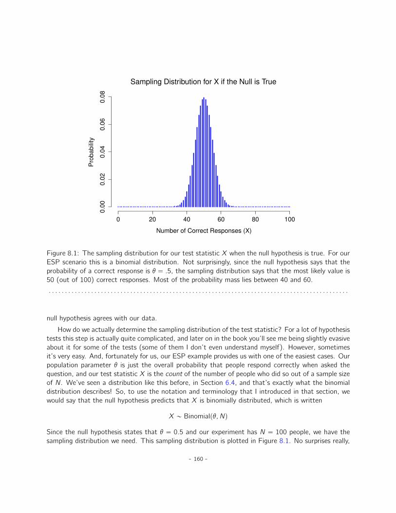
0 20 40 60 80 100

0.0

00

.02

0.0

40

.06

0.0

8

Sampling Distribution for X if the Null is True

Number of Correct Responses (X)

Pro

ba

bili

ty

Figure 8.1: The sampling distribution for our test statistic X when the null hypothesis is true. For ourESP scenario this is a binomial distribution. Not surprisingly, since the null hypothesis says that theprobability of a correct response is θ “ .5, the sampling distribution says that the most likely value is50 (out of 100) correct responses. Most of the probability mass lies between 40 and 60.

. . . . . . . . . . . . . . . . . . . . . . . . . . . . . . . . . . . . . . . . . . . . . . . . . . . . . . . . . . . . . . . . . . . . . . . . . . . . . . . . . . . . . . . . . . . .

null hypothesis agrees with our data.

How do we actually determine the sampling distribution of the test statistic? For a lot of hypothesistests this step is actually quite complicated, and later on in the book you’ll see me being slightly evasiveabout it for some of the tests (some of them I don’t even understand myself). However, sometimesit’s very easy. And, fortunately for us, our ESP example provides us with one of the easiest cases. Ourpopulation parameter θ is just the overall probability that people respond correctly when asked thequestion, and our test statistic X is the count of the number of people who did so out of a sample sizeof N. We’ve seen a distribution like this before, in Section 6.4, and that’s exactly what the binomialdistribution describes! So, to use the notation and terminology that I introduced in that section, wewould say that the null hypothesis predicts that X is binomially distributed, which is written

X „ Binomialpθ, Nq

Since the null hypothesis states that θ “ 0.5 and our experiment has N “ 100 people, we have thesampling distribution we need. This sampling distribution is plotted in Figure 8.1. No surprises really,

- 160 -

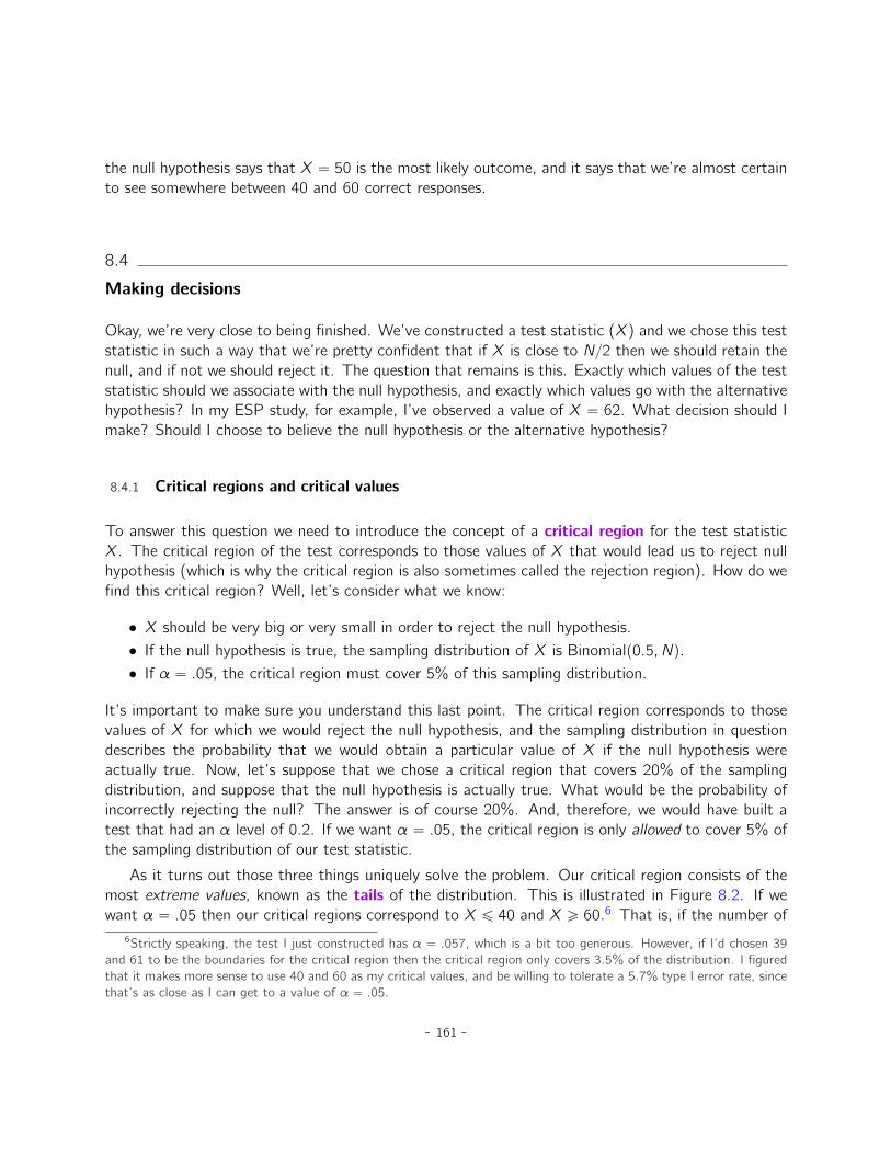
the null hypothesis says that X “ 50 is the most likely outcome, and it says that we’re almost certainto see somewhere between 40 and 60 correct responses.

8.4

Making decisions

Okay, we’re very close to being finished. We’ve constructed a test statistic (X) and we chose this teststatistic in such a way that we’re pretty confident that if X is close to N{2 then we should retain thenull, and if not we should reject it. The question that remains is this. Exactly which values of the teststatistic should we associate with the null hypothesis, and exactly which values go with the alternativehypothesis? In my ESP study, for example, I’ve observed a value of X “ 62. What decision should Imake? Should I choose to believe the null hypothesis or the alternative hypothesis?

8.4.1 Critical regions and critical values

To answer this question we need to introduce the concept of a critical region for the test statisticX. The critical region of the test corresponds to those values of X that would lead us to reject nullhypothesis (which is why the critical region is also sometimes called the rejection region). How do wefind this critical region? Well, let’s consider what we know:

• X should be very big or very small in order to reject the null hypothesis.• If the null hypothesis is true, the sampling distribution of X is Binomialp0.5, Nq.• If α “ .05, the critical region must cover 5% of this sampling distribution.

It’s important to make sure you understand this last point. The critical region corresponds to thosevalues of X for which we would reject the null hypothesis, and the sampling distribution in questiondescribes the probability that we would obtain a particular value of X if the null hypothesis wereactually true. Now, let’s suppose that we chose a critical region that covers 20% of the samplingdistribution, and suppose that the null hypothesis is actually true. What would be the probability ofincorrectly rejecting the null? The answer is of course 20%. And, therefore, we would have built atest that had an α level of 0.2. If we want α “ .05, the critical region is only allowed to cover 5% ofthe sampling distribution of our test statistic.

As it turns out those three things uniquely solve the problem. Our critical region consists of themost extreme values, known as the tails of the distribution. This is illustrated in Figure 8.2. If wewant α “ .05 then our critical regions correspond to X ď 40 and X ě 60.6 That is, if the number of

6Strictly speaking, the test I just constructed has α “ .057, which is a bit too generous. However, if I’d chosen 39and 61 to be the boundaries for the critical region then the critical region only covers 3.5% of the distribution. I figuredthat it makes more sense to use 40 and 60 as my critical values, and be willing to tolerate a 5.7% type I error rate, sincethat’s as close as I can get to a value of α “ .05.

- 161 -

0 20 40 60 80 100


lower critical region(2.5% of the distribution)

upper critical region(2.5% of the distribution)

Critical Regions for a Two−Sided Test

Figure 8.2: The critical region associated with the hypothesis test for the ESP study, for a hypothesistest with a significance level of α “ .05. The plot shows the sampling distribution of X under thenull hypothesis (i.e., same as Figure 8.1). The grey bars correspond to those values of X for whichwe would retain the null hypothesis. The blue (darker shaded) bars show the critical region, thosevalues of X for which we would reject the null. Because the alternative hypothesis is two sided (i.e.,allows both θ ă .5 and θ ą .5), the critical region covers both tails of the distribution. To ensure anα level of .05, we need to ensure that each of the two regions encompasses 2.5% of the samplingdistribution.

. . . . . . . . . . . . . . . . . . . . . . . . . . . . . . . . . . . . . . . . . . . . . . . . . . . . . . . . . . . . . . . . . . . . . . . . . . . . . . . . . . . . . . . . . . . .

people saying “true” is between 41 and 59, then we should retain the null hypothesis. If the number isbetween 0 to 40, or between 60 to 100, then we should reject the null hypothesis. The numbers 40and 60 are often referred to as the critical values since they define the edges of the critical region.

- 162 -

At this point, our hypothesis test is essentially complete:

1. (1) we choose an α level (e.g., α “ .05;2. (2) come up with some test statistic (e.g., X) that does a good job (in some meaningful sense)

of comparing H0 to H1;3. (3) figure out the sampling distribution of the test statistic on the assumption that the null

hypothesis is true (in this case, binomial); and then4. (4) calculate the critical region that produces an appropriate α level (0-40 and 60-100).

All that we have to do now is calculate the value of the test statistic for the real data (e.g., X “ 62)and then compare it to the critical values to make our decision. Since 62 is greater than the criticalvalue of 60 we would reject the null hypothesis. Or, to phrase it slightly differently, we say that thetest has produced a statistically significant result.

8.4.2 A note on statistical “significance”

Like other occult techniques of divination, the statistical method has a private jargondeliberately contrived to obscure its methods from non-practitioners.

– Attributed to G. O. Ashley7

A very brief digression is in order at this point, regarding the word “significant”. The concept ofstatistical significance is actually a very simple one, but has a very unfortunate name. If the dataallow us to reject the null hypothesis, we say that “the result is statistically significant”, which is oftenshortened to “the result is significant”. This terminology is rather old and dates back to a time when“significant” just meant something like “indicated”, rather than its modern meaning which is muchcloser to “important”. As a result, a lot of modern readers get very confused when they start learningstatistics because they think that a “significant result” must be an important one. It doesn’t mean thatat all. All that “statistically significant” means is that the data allowed us to reject a null hypothesis.Whether or not the result is actually important in the real world is a very different question, anddepends on all sorts of other things.

8.4.3 The difference between one sided and two sided tests

There’s one more thing I want to point out about the hypothesis test that I’ve just constructed. Ifwe take a moment to think about the statistical hypotheses I’ve been using,

H0 : θ “ .5

H1 : θ ‰ .5

7The internet seems fairly convinced that Ashley said this, though I can’t for the life of me find anyone willing to givea source for the claim.

- 163 -

we notice that the alternative hypothesis covers both the possibility that θ ă .5 and the possibilitythat θ ą .5. This makes sense if I really think that ESP could produce either better-than-chanceperformance or worse-than-chance performance (and there are some people who think that). Instatistical language this is an example of a two-sided test. It’s called this because the alternativehypothesis covers the area on both “sides” of the null hypothesis, and as a consequence the criticalregion of the test covers both tails of the sampling distribution (2.5% on either side if α “ .05), asillustrated earlier in Figure 8.2.

However, that’s not the only possibility. I might only be willing to believe in ESP if it producesbetter than chance performance. If so, then my alternative hypothesis would only covers the possibilitythat θ ą .5, and as a consequence the null hypothesis now becomes θ ď .5

H0 : θ ď .5

H1 : θ ą .5

When this happens, we have what’s called a one-sided test and the critical region only covers onetail of the sampling distribution. This is illustrated in Figure 8.3.

8.5

The p value of a test

In one sense, our hypothesis test is complete. We’ve constructed a test statistic, figured out itssampling distribution if the null hypothesis is true, and then constructed the critical region for thetest. Nevertheless, I’ve actually omitted the most important number of all, the p value. It is tothis topic that we now turn. There are two somewhat different ways of interpreting a p value, oneproposed by Sir Ronald Fisher and the other by Jerzy Neyman. Both versions are legitimate, thoughthey reflect very different ways of thinking about hypothesis tests. Most introductory textbooks tendto give Fisher’s version only, but I think that’s a bit of a shame. To my mind, Neyman’s version iscleaner and actually better reflects the logic of the null hypothesis test. You might disagree though,so I’ve included both. I’ll start with Neyman’s version.

8.5.1 A softer view of decision making

One problem with the hypothesis testing procedure that I’ve described is that it makes no distinctionat all between a result that is “barely significant” and those that are “highly significant”. For instance,in my ESP study the data I obtained only just fell inside the critical region, so I did get a significanteffect but it was a pretty near thing. In contrast, suppose that I’d run a study in which X “ 97 outof my N “ 100 participants got the answer right. This would obviously be significant too but mya much larger margin, such that there’s really no ambiguity about this at all. The procedure that Ihave already described makes no distinction between the two. If I adopt the standard convention ofallowing α “ .05 as my acceptable Type I error rate, then both of these are significant results.

- 164 -

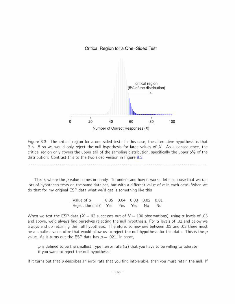
0 20 40 60 80 100


critical region(5% of the distribution)

Critical Region for a One−Sided Test

Figure 8.3: The critical region for a one sided test. In this case, the alternative hypothesis is thatθ ą .5 so we would only reject the null hypothesis for large values of X. As a consequence, thecritical region only covers the upper tail of the sampling distribution, specifically the upper 5% of thedistribution. Contrast this to the two-sided version in Figure 8.2.

. . . . . . . . . . . . . . . . . . . . . . . . . . . . . . . . . . . . . . . . . . . . . . . . . . . . . . . . . . . . . . . . . . . . . . . . . . . . . . . . . . . . . . . . . . . .

This is where the p value comes in handy. To understand how it works, let’s suppose that we ranlots of hypothesis tests on the same data set, but with a different value of α in each case. When wedo that for my original ESP data what we’d get is something like this

Value of α 0.05 0.04 0.03 0.02 0.01Reject the null? Yes Yes Yes No No

When we test the ESP data (X “ 62 successes out of N “ 100 observations), using α levels of .03and above, we’d always find ourselves rejecting the null hypothesis. For α levels of .02 and below wealways end up retaining the null hypothesis. Therefore, somewhere between .02 and .03 there mustbe a smallest value of α that would allow us to reject the null hypothesis for this data. This is the pvalue. As it turns out the ESP data has p “ .021. In short,

p is defined to be the smallest Type I error rate (α) that you have to be willing to tolerateif you want to reject the null hypothesis.

If it turns out that p describes an error rate that you find intolerable, then you must retain the null. If

- 165 -

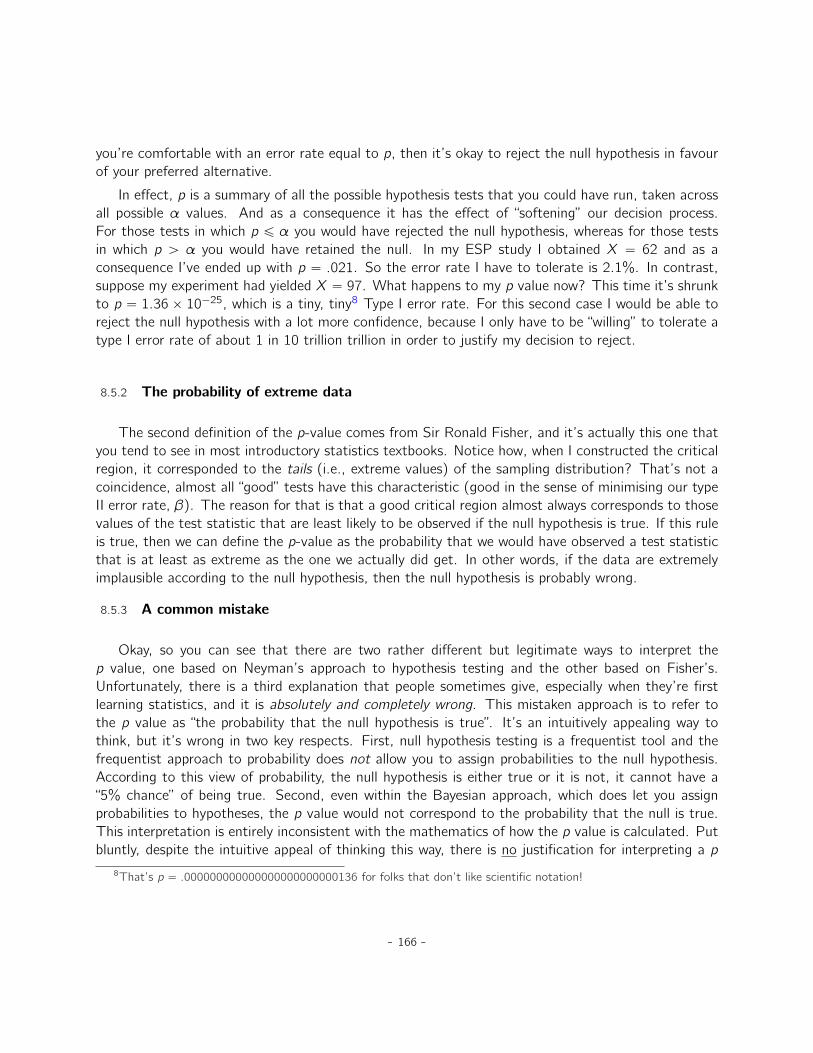
you’re comfortable with an error rate equal to p, then it’s okay to reject the null hypothesis in favourof your preferred alternative.

In effect, p is a summary of all the possible hypothesis tests that you could have run, taken acrossall possible α values. And as a consequence it has the effect of “softening” our decision process.For those tests in which p ď α you would have rejected the null hypothesis, whereas for those testsin which p ą α you would have retained the null. In my ESP study I obtained X “ 62 and as aconsequence I’ve ended up with p “ .021. So the error rate I have to tolerate is 2.1%. In contrast,suppose my experiment had yielded X “ 97. What happens to my p value now? This time it’s shrunkto p “ 1.36ˆ 10´25, which is a tiny, tiny8 Type I error rate. For this second case I would be able toreject the null hypothesis with a lot more confidence, because I only have to be “willing” to tolerate atype I error rate of about 1 in 10 trillion trillion in order to justify my decision to reject.

8.5.2 The probability of extreme data

The second definition of the p-value comes from Sir Ronald Fisher, and it’s actually this one thatyou tend to see in most introductory statistics textbooks. Notice how, when I constructed the criticalregion, it corresponded to the tails (i.e., extreme values) of the sampling distribution? That’s not acoincidence, almost all “good” tests have this characteristic (good in the sense of minimising our typeII error rate, β). The reason for that is that a good critical region almost always corresponds to thosevalues of the test statistic that are least likely to be observed if the null hypothesis is true. If this ruleis true, then we can define the p-value as the probability that we would have observed a test statisticthat is at least as extreme as the one we actually did get. In other words, if the data are extremelyimplausible according to the null hypothesis, then the null hypothesis is probably wrong.

8.5.3 A common mistake

Okay, so you can see that there are two rather different but legitimate ways to interpret thep value, one based on Neyman’s approach to hypothesis testing and the other based on Fisher’s.Unfortunately, there is a third explanation that people sometimes give, especially when they’re firstlearning statistics, and it is absolutely and completely wrong. This mistaken approach is to refer tothe p value as “the probability that the null hypothesis is true”. It’s an intuitively appealing way tothink, but it’s wrong in two key respects. First, null hypothesis testing is a frequentist tool and thefrequentist approach to probability does not allow you to assign probabilities to the null hypothesis.According to this view of probability, the null hypothesis is either true or it is not, it cannot have a“5% chance” of being true. Second, even within the Bayesian approach, which does let you assignprobabilities to hypotheses, the p value would not correspond to the probability that the null is true.This interpretation is entirely inconsistent with the mathematics of how the p value is calculated. Putbluntly, despite the intuitive appeal of thinking this way, there is no justification for interpreting a p

8That’s p “ .000000000000000000000000136 for folks that don’t like scientific notation!

- 166 -

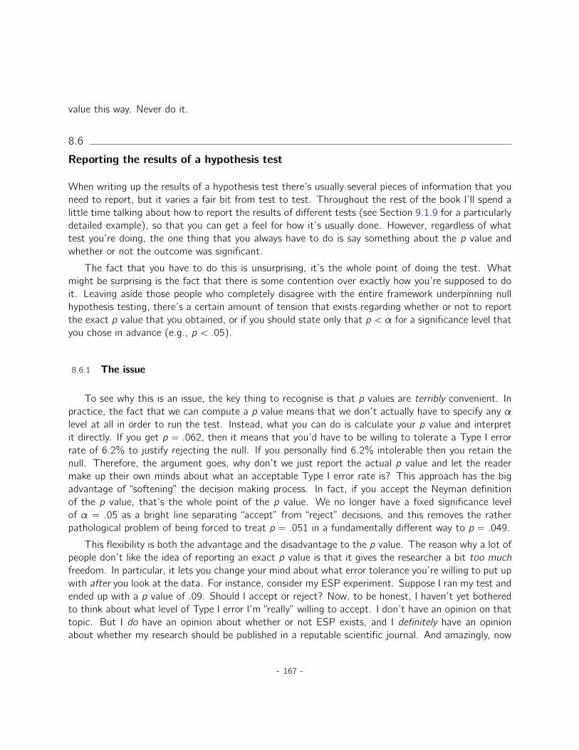
value this way. Never do it.

8.6

Reporting the results of a hypothesis test

When writing up the results of a hypothesis test there’s usually several pieces of information that youneed to report, but it varies a fair bit from test to test. Throughout the rest of the book I’ll spend alittle time talking about how to report the results of different tests (see Section 9.1.9 for a particularlydetailed example), so that you can get a feel for how it’s usually done. However, regardless of whattest you’re doing, the one thing that you always have to do is say something about the p value andwhether or not the outcome was significant.

The fact that you have to do this is unsurprising, it’s the whole point of doing the test. Whatmight be surprising is the fact that there is some contention over exactly how you’re supposed to doit. Leaving aside those people who completely disagree with the entire framework underpinning nullhypothesis testing, there’s a certain amount of tension that exists regarding whether or not to reportthe exact p value that you obtained, or if you should state only that p ă α for a significance level thatyou chose in advance (e.g., p ă .05).

8.6.1 The issue

To see why this is an issue, the key thing to recognise is that p values are terribly convenient. Inpractice, the fact that we can compute a p value means that we don’t actually have to specify any αlevel at all in order to run the test. Instead, what you can do is calculate your p value and interpretit directly. If you get p “ .062, then it means that you’d have to be willing to tolerate a Type I errorrate of 6.2% to justify rejecting the null. If you personally find 6.2% intolerable then you retain thenull. Therefore, the argument goes, why don’t we just report the actual p value and let the readermake up their own minds about what an acceptable Type I error rate is? This approach has the bigadvantage of “softening” the decision making process. In fact, if you accept the Neyman definitionof the p value, that’s the whole point of the p value. We no longer have a fixed significance levelof α “ .05 as a bright line separating “accept” from “reject” decisions, and this removes the ratherpathological problem of being forced to treat p “ .051 in a fundamentally different way to p “ .049.

This flexibility is both the advantage and the disadvantage to the p value. The reason why a lot ofpeople don’t like the idea of reporting an exact p value is that it gives the researcher a bit too muchfreedom. In particular, it lets you change your mind about what error tolerance you’re willing to put upwith after you look at the data. For instance, consider my ESP experiment. Suppose I ran my test andended up with a p value of .09. Should I accept or reject? Now, to be honest, I haven’t yet botheredto think about what level of Type I error I’m “really” willing to accept. I don’t have an opinion on thattopic. But I do have an opinion about whether or not ESP exists, and I definitely have an opinionabout whether my research should be published in a reputable scientific journal. And amazingly, now

- 167 -

that I’ve looked at the data I’m starting to think that a 9% error rate isn’t so bad, especially whencompared to how annoying it would be to have to admit to the world that my experiment has failed.So, to avoid looking like I just made it up after the fact, I now say that my α is .1, with the argumentthat a 10% type I error rate isn’t too bad and at that level my test is significant! I win.

In other words, the worry here is that I might have the best of intentions, and be the most honestof people, but the temptation to just “shade” things a little bit here and there is really, really strong.As anyone who has ever run an experiment can attest, it’s a long and difficult process and you oftenget very attached to your hypotheses. It’s hard to let go and admit the experiment didn’t find whatyou wanted it to find. And that’s the danger here. If we use the “raw” p-value, people will startinterpreting the data in terms of what they want to believe, not what the data are actually sayingand, if we allow that, why are we even bothering to do science at all? Why not let everyone believewhatever they like about anything, regardless of what the facts are? Okay, that’s a bit extreme, butthat’s where the worry comes from. According to this view, you really must specify your α valuein advance and then only report whether the test was significant or not. It’s the only way to keepourselves honest.

8.6.2 Two proposed solutions

In practice, it’s pretty rare for a researcher to specify a single α level ahead of time. Instead,the convention is that scientists rely on three standard significance levels: .05, .01 and .001. Whenreporting your results, you indicate which (if any) of these significance levels allow you to reject thenull hypothesis. This is summarised in Table 8.1. This allows us to soften the decision rule a littlebit, since p ă .01 implies that the data meet a stronger evidential standard than p ă .05 would.Nevertheless, since these levels are fixed in advance by convention, it does prevent people choosingtheir α level after looking at the data.

Nevertheless, quite a lot of people still prefer to report exact p values. To many people, theadvantage of allowing the reader to make up their own mind about how to interpret p “ .06 outweighsany disadvantages. In practice, however, even among those researchers who prefer exact p values itis quite common to just write p ă .001 instead of reporting an exact value for small p. This is inpart because a lot of software doesn’t actually print out the p value when it’s that small (e.g., SPSSjust writes p “ .000 whenever p ă .001), and in part because a very small p value can be kind ofmisleading. The human mind sees a number like .0000000001 and it’s hard to suppress the gut feelingthat the evidence in favour of the alternative hypothesis is a near certainty. In practice however, this isusually wrong. Life is a big, messy, complicated thing, and every statistical test ever invented relies onsimplifications, approximations and assumptions. As a consequence, it’s probably not reasonable towalk away from any statistical analysis with a feeling of confidence stronger than p ă .001 implies. Inother words, p ă .001 is really code for “as far as this test is concerned, the evidence is overwhelming.”

In light of all this, you might be wondering exactly what you should do. There’s a fair bit ofcontradictory advice on the topic, with some people arguing that you should report the exact p value,and other people arguing that you should use the tiered approach illustrated in Table 8.1. As a result,

- 168 -

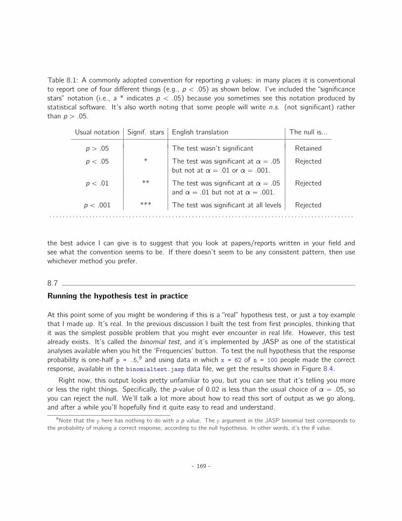
Table 8.1: A commonly adopted convention for reporting p values: in many places it is conventionalto report one of four different things (e.g., p ă .05) as shown below. I’ve included the “significancestars” notation (i.e., a * indicates p ă .05) because you sometimes see this notation produced bystatistical software. It’s also worth noting that some people will write n.s. (not significant) ratherthan p ą .05.

Usual notation Signif. stars English translation The null is...

p ą .05 The test wasn’t significant Retained

p ă .05 * The test was significant at α “ .05 Rejectedbut not at α “ .01 or α “ .001.

p ă .01 ** The test was significant at α “ .05 Rejectedand α “ .01 but not at α “ .001.

p ă .001 *** The test was significant at all levels Rejected. . . . . . . . . . . . . . . . . . . . . . . . . . . . . . . . . . . . . . . . . . . . . . . . . . . . . . . . . . . . . . . . . . . . . . . . . . . . . . . . . . . . . . . . . . . .

the best advice I can give is to suggest that you look at papers/reports written in your field andsee what the convention seems to be. If there doesn’t seem to be any consistent pattern, then usewhichever method you prefer.

8.7

Running the hypothesis test in practice

At this point some of you might be wondering if this is a “real” hypothesis test, or just a toy examplethat I made up. It’s real. In the previous discussion I built the test from first principles, thinking thatit was the simplest possible problem that you might ever encounter in real life. However, this testalready exists. It’s called the binomial test, and it’s implemented by JASP as one of the statisticalanalyses available when you hit the ‘Frequencies’ button. To test the null hypothesis that the responseprobability is one-half p = .5,9 and using data in which x = 62 of n = 100 people made the correctresponse, available in the binomialtest.jasp data file, we get the results shown in Figure 8.4.

Right now, this output looks pretty unfamiliar to you, but you can see that it’s telling you moreor less the right things. Specifically, the p-value of 0.02 is less than the usual choice of α “ .05, soyou can reject the null. We’ll talk a lot more about how to read this sort of output as we go along,and after a while you’ll hopefully find it quite easy to read and understand.

9Note that the p here has nothing to do with a p value. The p argument in the JASP binomial test corresponds tothe probability of making a correct response, according to the null hypothesis. In other words, it’s the θ value.

- 169 -

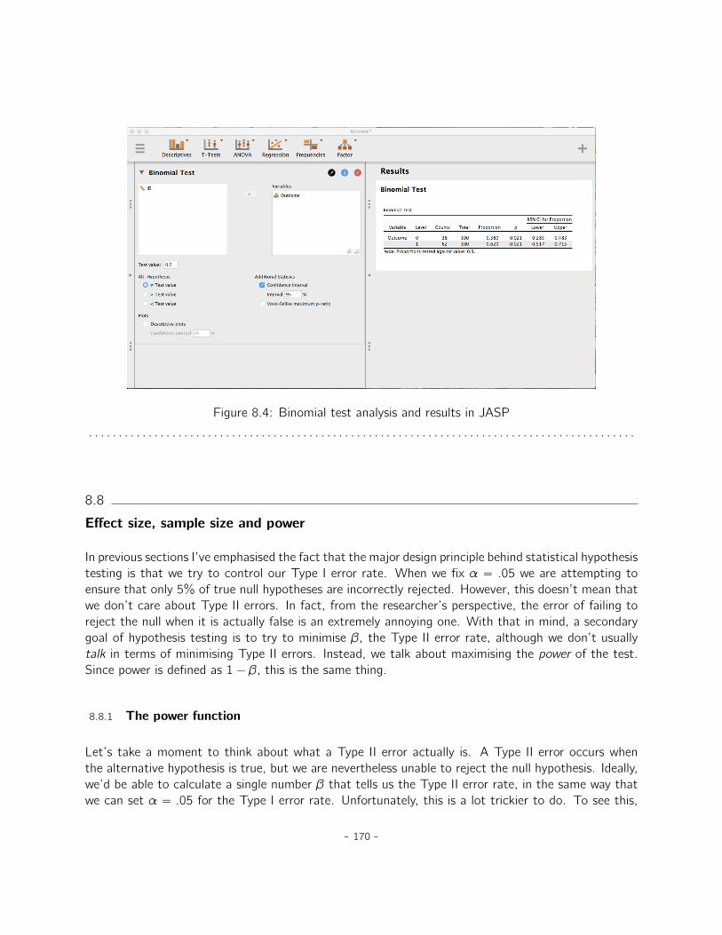
Figure 8.4: Binomial test analysis and results in JASP

. . . . . . . . . . . . . . . . . . . . . . . . . . . . . . . . . . . . . . . . . . . . . . . . . . . . . . . . . . . . . . . . . . . . . . . . . . . . . . . . . . . . . . . . . . . .

8.8

Effect size, sample size and power

In previous sections I’ve emphasised the fact that the major design principle behind statistical hypothesistesting is that we try to control our Type I error rate. When we fix α “ .05 we are attempting toensure that only 5% of true null hypotheses are incorrectly rejected. However, this doesn’t mean thatwe don’t care about Type II errors. In fact, from the researcher’s perspective, the error of failing toreject the null when it is actually false is an extremely annoying one. With that in mind, a secondarygoal of hypothesis testing is to try to minimise β, the Type II error rate, although we don’t usuallytalk in terms of minimising Type II errors. Instead, we talk about maximising the power of the test.Since power is defined as 1´ β, this is the same thing.

8.8.1 The power function

Let’s take a moment to think about what a Type II error actually is. A Type II error occurs whenthe alternative hypothesis is true, but we are nevertheless unable to reject the null hypothesis. Ideally,we’d be able to calculate a single number β that tells us the Type II error rate, in the same way thatwe can set α “ .05 for the Type I error rate. Unfortunately, this is a lot trickier to do. To see this,

- 170 -

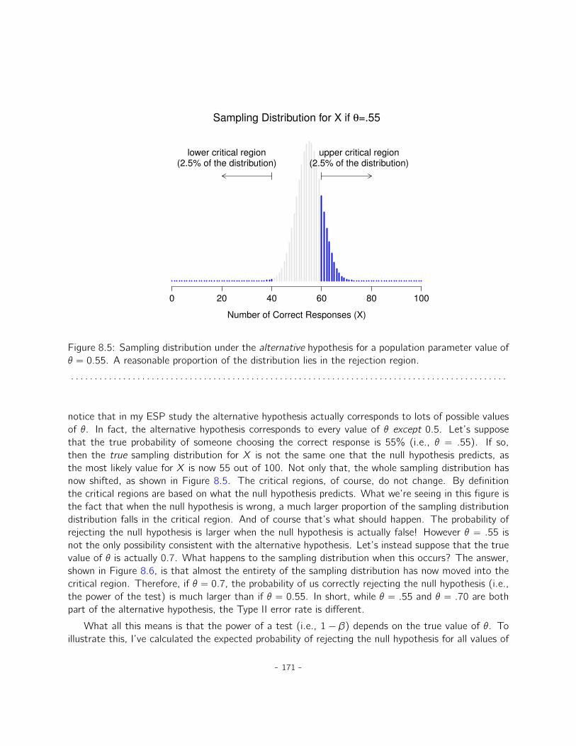
0 20 40 60 80 100




Sampling Distribution for X if θ=.55

Figure 8.5: Sampling distribution under the alternative hypothesis for a population parameter value ofθ “ 0.55. A reasonable proportion of the distribution lies in the rejection region.

. . . . . . . . . . . . . . . . . . . . . . . . . . . . . . . . . . . . . . . . . . . . . . . . . . . . . . . . . . . . . . . . . . . . . . . . . . . . . . . . . . . . . . . . . . . .

notice that in my ESP study the alternative hypothesis actually corresponds to lots of possible valuesof θ. In fact, the alternative hypothesis corresponds to every value of θ except 0.5. Let’s supposethat the true probability of someone choosing the correct response is 55% (i.e., θ “ .55). If so,then the true sampling distribution for X is not the same one that the null hypothesis predicts, asthe most likely value for X is now 55 out of 100. Not only that, the whole sampling distribution hasnow shifted, as shown in Figure 8.5. The critical regions, of course, do not change. By definitionthe critical regions are based on what the null hypothesis predicts. What we’re seeing in this figure isthe fact that when the null hypothesis is wrong, a much larger proportion of the sampling distributiondistribution falls in the critical region. And of course that’s what should happen. The probability ofrejecting the null hypothesis is larger when the null hypothesis is actually false! However θ “ .55 isnot the only possibility consistent with the alternative hypothesis. Let’s instead suppose that the truevalue of θ is actually 0.7. What happens to the sampling distribution when this occurs? The answer,shown in Figure 8.6, is that almost the entirety of the sampling distribution has now moved into thecritical region. Therefore, if θ “ 0.7, the probability of us correctly rejecting the null hypothesis (i.e.,the power of the test) is much larger than if θ “ 0.55. In short, while θ “ .55 and θ “ .70 are bothpart of the alternative hypothesis, the Type II error rate is different.

What all this means is that the power of a test (i.e., 1 ´ β) depends on the true value of θ. Toillustrate this, I’ve calculated the expected probability of rejecting the null hypothesis for all values of

- 171 -

0 20 40 60 80 100




Sampling Distribution for X if θ=.70

Figure 8.6: Sampling distribution under the alternative hypothesis for a population parameter value ofθ “ 0.70. Almost all of the distribution lies in the rejection region.

. . . . . . . . . . . . . . . . . . . . . . . . . . . . . . . . . . . . . . . . . . . . . . . . . . . . . . . . . . . . . . . . . . . . . . . . . . . . . . . . . . . . . . . . . . . .

θ, and plotted it in Figure 8.7. This plot describes what is usually called the power function of thetest. It’s a nice summary of how good the test is, because it actually tells you the power (1´ β) forall possible values of θ. As you can see, when the true value of θ is very close to 0.5, the power ofthe test drops very sharply, but when it is further away, the power is large.

8.8.2 Effect size

Since all models are wrong the scientist must be alert to what is importantly wrong. It isinappropriate to be concerned with mice when there are tigers abroad

– George Box (Box 1976, p. 792)

The plot shown in Figure 8.7 captures a fairly basic point about hypothesis testing. If the truestate of the world is very different from what the null hypothesis predicts then your power will be veryhigh, but if the true state of the world is similar to the null (but not identical) then the power ofthe test is going to be very low. Therefore, it’s useful to be able to have some way of quantifyinghow “similar” the true state of the world is to the null hypothesis. A statistic that does this is calleda measure of effect size (e.g., Cohen 1988; Ellis 2010). Effect size is defined slightly differently in

- 172 -

0.0 0.2 0.4 0.6 0.8 1.0

0.0

0.2

0.4

0.6

0.8

1.0

Power Function for the Test (N=100)

True Value of θ

Pro

ba

bili

ty o

f R

eje

ctin

g t

he

Nu

ll

Figure 8.7: The probability that we will reject the null hypothesis, plotted as a function of the truevalue of θ. Obviously, the test is more powerful (greater chance of correct rejection) if the true valueof θ is very different from the value that the null hypothesis specifies (i.e., θ “ .5). Notice that whenθ actually is equal to .5 (plotted as a black dot), the null hypothesis is in fact true and rejecting thenull hypothesis in this instance would be a Type I error.

. . . . . . . . . . . . . . . . . . . . . . . . . . . . . . . . . . . . . . . . . . . . . . . . . . . . . . . . . . . . . . . . . . . . . . . . . . . . . . . . . . . . . . . . . . . .

different contexts (and so this section just talks in general terms) but the qualitative idea that it triesto capture is always the same. How big is the difference between the true population parameters andthe parameter values that are assumed by the null hypothesis? In our ESP example, if we let θ0 “ 0.5

denote the value assumed by the null hypothesis and let θ denote the true value, then a simple measureof effect size could be something like the difference between the true value and null (i.e., θ ´ θ0), orpossibly just the magnitude of this difference, abspθ ´ θ0q.

Why calculate effect size? Let’s assume that you’ve run your experiment, collected the data, andgotten a significant effect when you ran your hypothesis test. Isn’t it enough just to say that you’vegotten a significant effect? Surely that’s the point of hypothesis testing? Well, sort of. Yes, the pointof doing a hypothesis test is to try to demonstrate that the null hypothesis is wrong, but that’s hardlythe only thing we’re interested in. If the null hypothesis claimed that θ “ .5 and we show that it’swrong, we’ve only really told half of the story. Rejecting the null hypothesis implies that we believethat θ ‰ .5, but there’s a big difference between θ “ .51 and θ “ .8. If we find that θ “ .8, then notonly have we found that the null hypothesis is wrong, it appears to be very wrong. On the other hand,suppose we’ve successfully rejected the null hypothesis, but it looks like the true value of θ is only .51

- 173 -

Table 8.2: A crude guide to understanding the relationship between statistical significance and effectsizes. Basically, if you don’t have a significant result then the effect size is pretty meaningless becauseyou don’t have any evidence that it’s even real. On the other hand, if you do have a significant effectbut your effect size is small then there’s a pretty good chance that your result (although real) isn’t allthat interesting. However, this guide is very crude. It depends a lot on what exactly you’re studying.Small effects can be of massive practical importance in some situations. So don’t take this table tooseriously. It’s a rough guide at best.

big effect size small effect sizesignificant result difference is real, and difference is real, but

of practical importance might not be interesting

non-significant result no effect observed no effect observed. . . . . . . . . . . . . . . . . . . . . . . . . . . . . . . . . . . . . . . . . . . . . . . . . . . . . . . . . . . . . . . . . . . . . . . . . . . . . . . . . . . . . . . . . . . .

(this would only be possible with a very large study). Sure, the null hypothesis is wrong but it’s notat all clear that we actually care because the effect size is so small. In the context of my ESP studywe might still care since any demonstration of real psychic powers would actually be pretty cool10,but in other contexts a 1% difference usually isn’t very interesting, even if it is a real difference. Forinstance, suppose we’re looking at differences in high school exam scores between males and femalesand it turns out that the female scores are 1% higher on average than the males. If I’ve got datafrom thousands of students then this difference will almost certainly be statistically significant, butregardless of how small the p value is it’s just not very interesting. You’d hardly want to go aroundproclaiming a crisis in boys education on the basis of such a tiny difference would you? It’s for thisreason that it is becoming more standard (slowly, but surely) to report some kind of standard measureof effect size along with the the results of the hypothesis test. The hypothesis test itself tells youwhether you should believe that the effect you have observed is real (i.e., not just due to chance),whereas the effect size tells you whether or not you should care.

8.8.3 Increasing the power of your study

Not surprisingly, scientists are fairly obsessed with maximising the power of their experiments. Wewant our experiments to work and so we want to maximise the chance of rejecting the null hypothesisif it is false (and of course we usually want to believe that it is false!). As we’ve seen, one factorthat influences power is the effect size. So the first thing you can do to increase your power is toincrease the effect size. In practice, what this means is that you want to design your study in such a

10Although in practice a very small effect size is worrying because even very minor methodological flaws might beresponsible for the effect, and in practice no experiment is perfect so there are always methodological issues to worryabout.

- 174 -

way that the effect size gets magnified. For instance, in my ESP study I might believe that psychicpowers work best in a quiet, darkened room with fewer distractions to cloud the mind. Therefore Iwould try to conduct my experiments in just such an environment. If I can strengthen people’s ESPabilities somehow then the true value of θ will go up11 and therefore my effect size will be larger. Inshort, clever experimental design is one way to boost power, because it can alter the effect size.

Unfortunately, it’s often the case that even with the best of experimental designs you may haveonly a small effect. Perhaps, for example, ESP really does exist but even under the best of conditionsit’s very very weak. Under those circumstances your best bet for increasing power is to increase thesample size. In general, the more observations that you have available, the more likely it is that youcan discriminate between two hypotheses. If I ran my ESP experiment with 10 participants and 7 ofthem correctly guessed the colour of the hidden card you wouldn’t be terribly impressed. But if I ranit with 10,000 participants, and 7,000 of them got the answer right, you would be much more likelyto think I had discovered something. In other words, power increases with the sample size. This isillustrated in Figure 8.8, which shows the power of the test for a true parameter of θ “ 0.7 for allsample sizes N from 1 to 100, where I’m assuming that the null hypothesis predicts that θ0 “ 0.5.

Because power is important, whenever you’re contemplating running an experiment it would bepretty useful to know how much power you’re likely to have. It’s never possible to know for sure sinceyou can’t possibly know what your real effect size is. However, it’s often (well, sometimes) possible toguess how big it should be. If so, you can guess what sample size you need! This idea is called poweranalysis, and if it’s feasible to do it then it’s very helpful. It can tell you something about whether youhave enough time or money to be able to run the experiment successfully. It’s increasingly common tosee people arguing that power analysis should be a required part of experimental design, so it’s worthknowing about. I don’t discuss power analysis in this book, however. This is partly for a boring reasonand partly for a substantive one. The boring reason is that I haven’t had time to write about poweranalysis yet. The substantive one is that I’m still a little suspicious of power analysis. Speaking as aresearcher, I have very rarely found myself in a position to be able to do one. It’s either the case that(a) my experiment is a bit non-standard and I don’t know how to define effect size properly, or (b) Iliterally have so little idea about what the effect size will be that I wouldn’t know how to interpret theanswers. Not only that, after extensive conversations with someone who does stats consulting for aliving (my wife, as it happens), I can’t help but notice that in practice the only time anyone ever asksher for a power analysis is when she’s helping someone write a grant application. In other words, theonly time any scientist ever seems to want a power analysis in real life is when they’re being forcedto do it by bureaucratic process. It’s not part of anyone’s day to day work. In short, I’ve always beenof the view that whilst power is an important concept, power analysis is not as useful as people makeit sound, except in the rare cases where (a) someone has figured out how to calculate power for your

11Notice that the true population parameter θ doesn’t necessarily correspond to an immutable fact of nature. In thiscontext θ is just the true probability that people would correctly guess the colour of the card in the other room. Assuch the population parameter can be influenced by all sorts of things. Of course, this is all on the assumption that ESPactually exists!

- 175 -

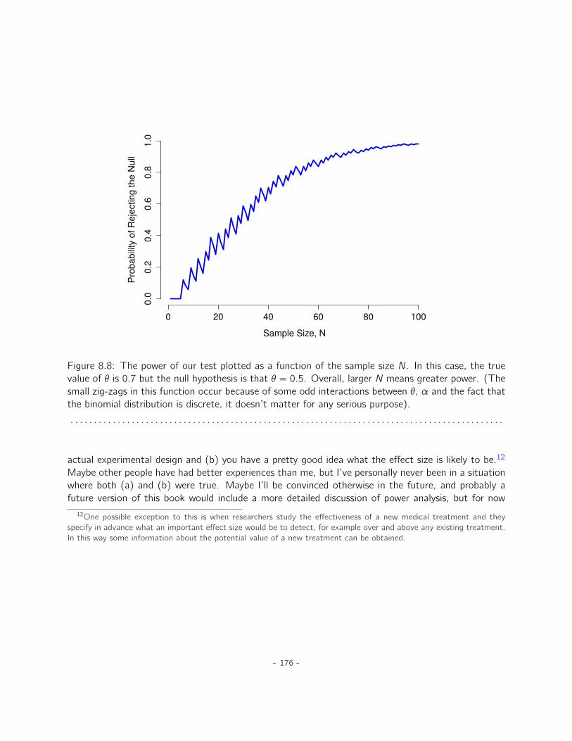
0 20 40 60 80 100

0.0

0.2

0.4

0.6

0.8

1.0

Sample Size, N

Pro

ba

bili

ty o

f R

eje

ctin

g t

he

Nu

ll

Figure 8.8: The power of our test plotted as a function of the sample size N. In this case, the truevalue of θ is 0.7 but the null hypothesis is that θ “ 0.5. Overall, larger N means greater power. (Thesmall zig-zags in this function occur because of some odd interactions between θ, α and the fact thatthe binomial distribution is discrete, it doesn’t matter for any serious purpose).

. . . . . . . . . . . . . . . . . . . . . . . . . . . . . . . . . . . . . . . . . . . . . . . . . . . . . . . . . . . . . . . . . . . . . . . . . . . . . . . . . . . . . . . . . . . .

actual experimental design and (b) you have a pretty good idea what the effect size is likely to be.12

Maybe other people have had better experiences than me, but I’ve personally never been in a situationwhere both (a) and (b) were true. Maybe I’ll be convinced otherwise in the future, and probably afuture version of this book would include a more detailed discussion of power analysis, but for now

12One possible exception to this is when researchers study the effectiveness of a new medical treatment and theyspecify in advance what an important effect size would be to detect, for example over and above any existing treatment.In this way some information about the potential value of a new treatment can be obtained.

- 176 -

this is about as much as I’m comfortable saying about the topic.

8.9

Some issues to consider

What I’ve described to you in this chapter is the orthodox framework for null hypothesis significancetesting (NHST). Understanding how NHST works is an absolute necessity because it has been thedominant approach to inferential statistics ever since it came to prominence in the early 20th century.It’s what the vast majority of working scientists rely on for their data analysis, so even if you hate ityou need to know it. However, the approach is not without problems. There are a number of quirksin the framework, historical oddities in how it came to be, theoretical disputes over whether or notthe framework is right, and a lot of practical traps for the unwary. I’m not going to go into a lot ofdetail on this topic, but I think it’s worth briefly discussing a few of these issues.

8.9.1 Neyman versus Fisher

The first thing you should be aware of is that orthodox NHST is actually a mash-up of two ratherdifferent approaches to hypothesis testing, one proposed by Sir Ronald Fisher and the other proposedby Jerzy Neyman (see Lehmann 2011, for a historical summary). The history is messy because Fisherand Neyman were real people whose opinions changed over time, and at no point did either of themoffer “the definitive statement” of how we should interpret their work many decades later. That said,here’s a quick summary of what I take these two approaches to be.

First, let’s talk about Fisher’s approach. As far as I can tell, Fisher assumed that you only had theone hypothesis (the null) and that what you want to do is find out if the null hypothesis is inconsistentwith the data. From his perspective, what you should do is check to see if the data are “sufficientlyunlikely” according to the null. In fact, if you remember back to our earlier discussion, that’s howFisher defines the p-value. According to Fisher, if the null hypothesis provided a very poor account ofthe data then you could safely reject it. But, since you don’t have any other hypotheses to compareit to, there’s no way of “accepting the alternative” because you don’t necessarily have an explicitlystated alternative. That’s more or less all there is to it.

In contrast, Neyman thought that the point of hypothesis testing was as a guide to action andhis approach was somewhat more formal than Fisher’s. His view was that there are multiple thingsthat you could do (accept the null or accept the alternative) and the point of the test was to tell youwhich one the data support. From this perspective, it is critical to specify your alternative hypothesisproperly. If you don’t know what the alternative hypothesis is, then you don’t know how powerful thetest is, or even which action makes sense. His framework genuinely requires a competition betweendifferent hypotheses. For Neyman, the p value didn’t directly measure the probability of the data(or data more extreme) under the null, it was more of an abstract description about which “possibletests” were telling you to accept the null, and which “possible tests” were telling you to accept the

- 177 -

alternative.

As you can see, what we have today is an odd mishmash of the two. We talk about having both anull hypothesis and an alternative (Neyman), but usually13 define the p value in terms of exreme data(Fisher), but we still have α values (Neyman). Some of the statistical tests have explicitly specifiedalternatives (Neyman) but others are quite vague about it (Fisher). And, according to some peopleat least, we’re not allowed to talk about accepting the alternative (Fisher). It’s a mess, but I hopethis at least explains why it’s a mess.

8.9.2 Bayesians versus frequentists

Earlier on in this chapter I was quite emphatic about the fact that you cannot interpret the pvalue as the probability that the null hypothesis is true. NHST is fundamentally a frequentist tool (seeChapter 6) and as such it does not allow you to assign probabilities to hypotheses. The null hypothesisis either true or it is not. The Bayesian approach to statistics interprets probability as a degree ofbelief, so it’s totally okay to say that there is a 10% chance that the null hypothesis is true. That’sjust a reflection of the degree of confidence that you have in this hypothesis. You aren’t allowed todo this within the frequentist approach. Remember, if you’re a frequentist, a probability can only bedefined in terms of what happens after a large number of independent replications (i.e., a long runfrequency). If this is your interpretation of probability, talking about the “probability” that the nullhypothesis is true is complete gibberish: a null hypothesis is either true or it is false. There’s no wayyou can talk about a long run frequency for this statement. To talk about “the probability of the nullhypothesis” is as meaningless as “the colour of freedom”. It doesn’t have one!

Most importantly, this isn’t a purely ideological matter. If you decide that you are a Bayesianand that you’re okay with making probability statements about hypotheses, you have to follow theBayesian rules for calculating those probabilities. I’ll talk more about this in Chapter 14, but for nowwhat I want to point out to you is the p value is a terrible approximation to the probability that H0

is true. If what you want to know is the probability of the null, then the p value is not what you’relooking for!

8.9.3 Traps

As you can see, the theory behind hypothesis testing is a mess, and even now there are argumentsin statistics about how it “should” work. However, disagreements among statisticians are not our realconcern here. Our real concern is practical data analysis. And while the “orthodox” approach to nullhypothesis significance testing has many drawbacks, even an unrepentant Bayesian like myself wouldagree that they can be useful if used responsibly. Most of the time they give sensible answers and youcan use them to learn interesting things. Setting aside the various ideologies and historical confusionsthat we’ve discussed, the fact remains that the biggest danger in all of statistics is thoughtlessness. I

13Although this book describes both Neyman’s and Fisher’s definition of the p value, most don’t. Most introductorytextbooks will only give you the Fisher version.

- 178 -

don’t mean stupidity, I literally mean thoughtlessness. The rush to interpret a result without spendingtime thinking through what each test actually says about the data, and checking whether that’sconsistent with how you’ve interpreted it. That’s where the biggest trap lies.

To give an example of this, consider the following example (see Gelman and Stern 2006). SupposeI’m running my ESP study and I’ve decided to analyse the data separately for the male participantsand the female participants. Of the male participants, 33 out of 50 guessed the colour of the cardcorrectly. This is a significant effect (p “ .03). Of the female participants, 29 out of 50 guessedcorrectly. This is not a significant effect (p “ .32). Upon observing this, it is extremely temptingfor people to start wondering why there is a difference between males and females in terms of theirpsychic abilities. However, this is wrong. If you think about it, we haven’t actually run a test thatexplicitly compares males to females. All we have done is compare males to chance (binomial testwas significant) and compared females to chance (binomial test was non significant). If we want toargue that there is a real difference between the males and the females, we should probably run a testof the null hypothesis that there is no difference! We can do that using a different hypothesis test,14

but when we do that it turns out that we have no evidence that males and females are significantlydifferent (p “ .54). Now do you think that there’s anything fundamentally different between thetwo groups? Of course not. What’s happened here is that the data from both groups (male andfemale) are pretty borderline. By pure chance one of them happened to end up on the magic side ofthe p “ .05 line, and the other one didn’t. That doesn’t actually imply that males and females aredifferent. This mistake is so common that you should always be wary of it. The difference betweensignificant and not-significant is not evidence of a real difference. If you want to say that there’s adifference between two groups, then you have to test for that difference!

The example above is just that, an example. I’ve singled it out because it’s such a common one,but the bigger picture is that data analysis can be tricky to get right. Think about what it is you wantto test, why you want to test it, and whether or not the answers that your test gives could possiblymake any sense in the real world.

8.10

Summary

Null hypothesis testing is one of the most ubiquitous elements to statistical theory. The vast majorityof scientific papers report the results of some hypothesis test or another. As a consequence it isalmost impossible to get by in science without having at least a cursory understanding of what ap-value means, making this one of the most important chapters in the book. As usual, I’ll end thechapter with a quick recap of the key ideas that we’ve talked about:

• Research hypotheses and statistical hypotheses. Null and alternative hypotheses. (Section 8.1).• Type 1 and Type 2 errors (Section 8.2)• Test statistics and sampling distributions (Section 8.3)

14In this case, the Pearson chi-square test of independence (Chapter 9)

- 179 -

• Hypothesis testing as a decision making process (Section 8.4)

• p-values as “soft” decisions (Section 8.5)

• Writing up the results of a hypothesis test (Section 8.6)

• Running the hypothesis test in practice (Section 8.7)

• Effect size and power (Section 8.8)

• A few issues to consider regarding hypothesis testing (Section 8.9)

Later in the book, in Chapter 14, I’ll revisit the theory of null hypothesis tests from a Bayesianperspective and introduce a number of new tools that you can use if you aren’t particularly fond ofthe orthodox approach. But for now, though, we’re done with the abstract statistical theory, and wecan start discussing specific data analysis tools.

- 180 -

Part IV.

Statistical tools

- 181 -

9. Categorical data analysis

Now that we’ve covered the basic theory behind hypothesis testing it’s time to start looking at specifictests that are commonly used in psychology. So where should we start? Not every textbook agreeson where to start, but I’m going to start with “χ2 tests” (this chapter, pronounced “chi-square”1) and“t-tests” (Chapter 10). Both of these tools are very frequently used in scientific practice, and whilstthey’re not as powerful as “regression” (Chapter 11) and “analysis of variance” (Chapter 12) they’remuch easier to understand.

The term “categorical data” is just another name for “nominal scale data”. It’s nothing that wehaven’t already discussed, it’s just that in the context of data analysis people tend to use the term“categorical data” rather than “nominal scale data”. I don’t know why. In any case, categorical dataanalysis refers to a collection of tools that you can use when your data are nominal scale. However,there are a lot of different tools that can be used for categorical data analysis, and this chapter coversonly a few of the more common ones.

9.1

The χ2 (chi-square) goodness-of-fit test

The χ2 goodness-of-fit test is one of the oldest hypothesis tests around. It was invented by KarlPearson around the turn of the century (Pearson 1900), with some corrections made later by SirRonald Fisher (Fisher 1922a). It tests whether an observed frequency distribution of a nominal variablematches an expected frequency distribution. For example, suppose a group of patients has beenundergoing an experimental treatment and have had their health assessed to see whether their conditionhas improved, stayed the same or worsened. A goodness-of-fit test could be used to determinewhether the numbers in each category - improved, no change, worsened - match the numbers thatwould be expected given the standard treatment option. Let’s think about this some more, with somepsychology.

1Also sometimes referred to as “chi-squared”

- 183 -

9.1.1 The cards data

Over the years there have been many studies showing that humans find it difficult to simulate ran-domness. Try as we might to “act” random, we think in terms of patterns and structure and so, whenasked to “do something at random”, what people actually do is anything but random. As a conse-quence, the study of human randomness (or non-randomness, as the case may be) opens up a lot ofdeep psychological questions about how we think about the world. With this in mind, let’s considera very simple study. Suppose I asked people to imagine a shuffled deck of cards, and mentally pickone card from this imaginary deck “at random”. After they’ve chosen one card I ask them to mentallyselect a second one. For both choices what we’re going to look at is the suit (hearts, clubs, spadesor diamonds) that people chose. After asking, say, N “ 200 people to do this, I’d like to look at thedata and figure out whether or not the cards that people pretended to select were really random. Thedata are contained in the randomness.csv file in which, when you open it up in JASP, you will seethree variables. These are: an id variable that assigns a unique identifier to each participant, and thetwo variables choice_1 and choice_2 that indicate the card suits that people chose.

For the moment, let’s just focus on the first choice that people made. We’ll use the Frequencytables option under ‘Descriptives’ - ‘Descriptive Statistics’ to count the number of times that weobserved people choosing each suit. This is what we get:

clubs diamonds hearts spades35 51 64 50

That little frequency table is quite helpful. Looking at it, there’s a bit of a hint that people mightbe more likely to select hearts than clubs, but it’s not completely obvious just from looking at itwhether that’s really true, or if this is just due to chance. So we’ll probably have to do some kind ofstatistical analysis to find out, which is what I’m going to talk about in the next section.

Excellent. From this point on, we’ll treat this table as the data that we’re looking to analyse.However, since I’m going to have to talk about this data in mathematical terms, it might be a goodidea to be clear about what the notation is. In mathematical notation, we shorten the human-readableword “observed” to the letter O, and we use subscripts to denote the position of the observation. Sothe second observation in our table is written as O2 in maths. The relationship between the Englishdescriptions and the mathematical symbols are illustrated below:

label index, i math. symbol the valueclubs, ♣ 1 O1 35

diamonds, ♦ 2 O2 51hearts, ♥ 3 O3 64spades, ♠ 4 O4 50

Hopefully that’s pretty clear. It’s also worth noting that mathematicians prefer to talk about generalrather than specific things, so you’ll also see the notationOi , which refers to the number of observations

- 184 -

that fall within the i-th category (where i could be 1, 2, 3 or 4). Finally, if we want to refer to theset of all observed frequencies, statisticians group all observed values into a vector2, which I’ll referto using boldface type as O.

O “ pO1, O2, O3, O4q

Again, this is nothing new or interesting. It’s just notation. If I say that O “ p35, 51, 64, 50q allI’m doing is describing the table of observed frequencies (i.e., observed), but I’m referring to it usingmathematical notation.

9.1.2 The null hypothesis and the alternative hypothesis

As the last section indicated, our research hypothesis is that “people don’t choose cards randomly”.What we’re going to want to do now is translate this into some statistical hypotheses and thenconstruct a statistical test of those hypotheses. The test that I’m going to describe to you is Pearson’sχ2 (chi-square) goodness-of-fit test, and as is so often the case we have to begin by carefullyconstructing our null hypothesis. In this case, it’s pretty easy. First, let’s state the null hypothesis inwords:

H0: All four suits are chosen with equal probability

Now, because this is statistics, we have to be able to say the same thing in a mathematical way. Todo this, let’s use the notation Pj to refer to the true probability that the j-th suit is chosen. If the nullhypothesis is true, then each of the four suits has a 25% chance of being selected. In other words,our null hypothesis claims that P1 “ .25, P2 “ .25, P3 “ .25 and finally that P4 “ .25. However,in the same way that we can group our observed frequencies into a vector O that summarises theentire data set, we can use P to refer to the probabilities that correspond to our null hypothesis. Soif I let the vector P “ pP1, P2, P3, P4q refer to the collection of probabilities that describe our nullhypothesis, then we have:

H0: P “ p.25, .25, .25, .25q

In this particular instance, our null hypothesis corresponds to a vector of probabilities P in which all ofthe probabilities are equal to one another. But this doesn’t have to be the case. For instance, if theexperimental task was for people to imagine they were drawing from a deck that had twice as manyclubs as any other suit, then the null hypothesis would correspond to something like P “ p.4, .2, .2, .2q.As long as the probabilities are all positive numbers, and they all sum to 1, then it’s a perfectlylegitimate choice for the null hypothesis. However, the most common use of the goodness-of-fit testis to test a null hypothesis that all of the categories are equally likely, so we’ll stick to that for ourexample.

2A vector is a sequence of data elements of the same basic type

- 185 -

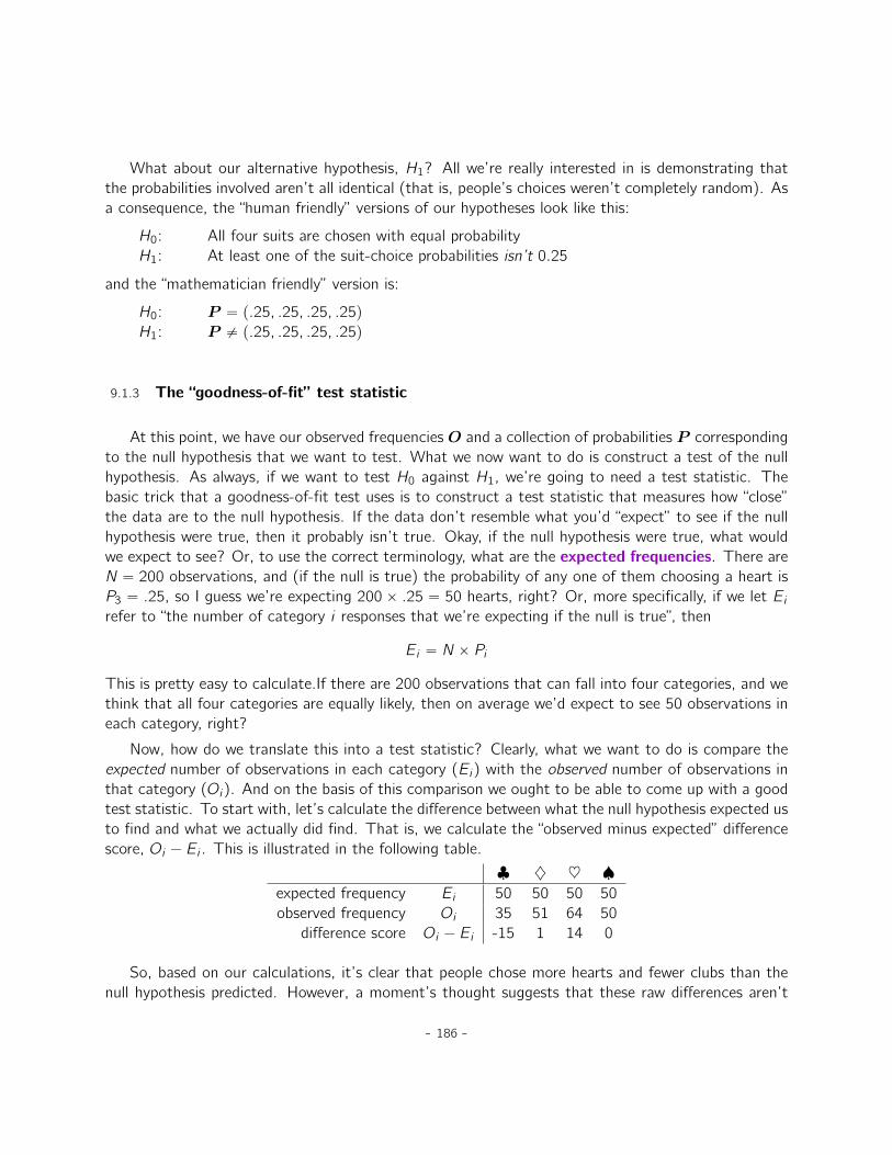
What about our alternative hypothesis, H1? All we’re really interested in is demonstrating thatthe probabilities involved aren’t all identical (that is, people’s choices weren’t completely random). Asa consequence, the “human friendly” versions of our hypotheses look like this:

H0: All four suits are chosen with equal probabilityH1: At least one of the suit-choice probabilities isn’t 0.25

and the “mathematician friendly” version is:

H0: P “ p.25, .25, .25, .25q

H1: P ‰ p.25, .25, .25, .25q

9.1.3 The “goodness-of-fit” test statistic

At this point, we have our observed frequencies O and a collection of probabilities P correspondingto the null hypothesis that we want to test. What we now want to do is construct a test of the nullhypothesis. As always, if we want to test H0 against H1, we’re going to need a test statistic. Thebasic trick that a goodness-of-fit test uses is to construct a test statistic that measures how “close”the data are to the null hypothesis. If the data don’t resemble what you’d “expect” to see if the nullhypothesis were true, then it probably isn’t true. Okay, if the null hypothesis were true, what wouldwe expect to see? Or, to use the correct terminology, what are the expected frequencies. There areN “ 200 observations, and (if the null is true) the probability of any one of them choosing a heart isP3 “ .25, so I guess we’re expecting 200ˆ .25 “ 50 hearts, right? Or, more specifically, if we let Eirefer to “the number of category i responses that we’re expecting if the null is true”, then

Ei “ N ˆ Pi

This is pretty easy to calculate.If there are 200 observations that can fall into four categories, and wethink that all four categories are equally likely, then on average we’d expect to see 50 observations ineach category, right?

Now, how do we translate this into a test statistic? Clearly, what we want to do is compare theexpected number of observations in each category (Ei) with the observed number of observations inthat category (Oi). And on the basis of this comparison we ought to be able to come up with a goodtest statistic. To start with, let’s calculate the difference between what the null hypothesis expected usto find and what we actually did find. That is, we calculate the “observed minus expected” differencescore, Oi ´ Ei . This is illustrated in the following table.

♣ ♦ ♥ ♠expected frequency Ei 50 50 50 50observed frequency Oi 35 51 64 50

difference score Oi ´ Ei -15 1 14 0

So, based on our calculations, it’s clear that people chose more hearts and fewer clubs than thenull hypothesis predicted. However, a moment’s thought suggests that these raw differences aren’t

- 186 -

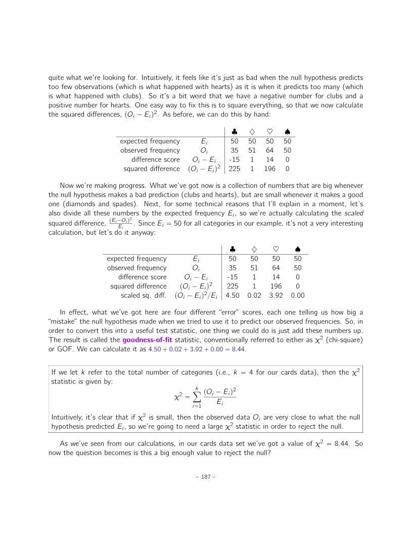
quite what we’re looking for. Intuitively, it feels like it’s just as bad when the null hypothesis predictstoo few observations (which is what happened with hearts) as it is when it predicts too many (whichis what happened with clubs). So it’s a bit weird that we have a negative number for clubs and apositive number for hearts. One easy way to fix this is to square everything, so that we now calculatethe squared differences, pOi ´ Eiq2. As before, we can do this by hand:


difference score Oi ´ Ei -15 1 14 0squared difference pOi ´ Eiq

2 225 1 196 0

Now we’re making progress. What we’ve got now is a collection of numbers that are big wheneverthe null hypothesis makes a bad prediction (clubs and hearts), but are small whenever it makes a goodone (diamonds and spades). Next, for some technical reasons that I’ll explain in a moment, let’salso divide all these numbers by the expected frequency Ei , so we’re actually calculating the scaledsquared difference, pEi´Oi q

2

Ei. Since Ei “ 50 for all categories in our example, it’s not a very interesting

calculation, but let’s do it anyway:


difference score Oi ´ Ei -15 1 14 0squared difference pOi ´ Eiq

2 225 1 196 0scaled sq. diff. pOi ´ Eiq

2{Ei 4.50 0.02 3.92 0.00

In effect, what we’ve got here are four different “error” scores, each one telling us how big a“mistake” the null hypothesis made when we tried to use it to predict our observed frequencies. So, inorder to convert this into a useful test statistic, one thing we could do is just add these numbers up.The result is called the goodness-of-fit statistic, conventionally referred to either as χ2 (chi-square)or GOF. We can calculate it as 4.50` 0.02` 3.92` 0.00 “ 8.44.

If we let k refer to the total number of categories (i.e., k “ 4 for our cards data), then the χ2

statistic is given by:

χ2 “

kÿ

i“1

pOi ´ Eiq2

Ei

Intuitively, it’s clear that if χ2 is small, then the observed data Oi are very close to what the nullhypothesis predicted Ei , so we’re going to need a large χ2 statistic in order to reject the null.

As we’ve seen from our calculations, in our cards data set we’ve got a value of χ2 “ 8.44. Sonow the question becomes is this a big enough value to reject the null?

- 187 -

9.1.4 The sampling distribution of the GOF statistic

To determine whether or not a particular value of χ2 is large enough to justify rejecting the nullhypothesis, we’re going to need to figure out what the sampling distribution for χ2 would be if the nullhypothesis were true. So that’s what I’m going to do in this section. I’ll show you in a fair amount ofdetail how this sampling distribution is constructed, and then, in the next section, use it to build up ahypothesis test. If you want to cut to the chase and are willing to take it on faith that the samplingdistribution is a χ2 (chi-square) distribution with k ´ 1 degrees of freedom, you can skip the rest ofthis section. However, if you want to understand why the goodness-of-fit test works the way it does,read on.

Okay, let’s suppose that the null hypothesis is actually true. If so, then the true probability thatan observation falls in the i-th category is Pi . After all, that’s pretty much the definition of our nullhypothesis. Let’s think about what this actually means. This is kind of like saying that “nature” makesthe decision about whether or not the observation ends up in category i by flipping a weighted coin(i.e., one where the probability of getting a head is Pj). And therefore we can think of our observedfrequency Oi by imagining that nature flipped N of these coins (one for each observation in the dataset), and exactly Oi of them came up heads. Obviously, this is a pretty weird way to think about theexperiment. But what it does (I hope) is remind you that we’ve actually seen this scenario before. It’sexactly the same set up that gave rise to the binomial distribution in Section 6.4. In other words, ifthe null hypothesis is true, then it follows that our observed frequencies were generated by samplingfrom a binomial distribution:

Oi „ BinomialpPi , Nq

Now, if you remember from our discussion of the central limit theorem (Section 7.3.3) the binomialdistribution starts to look pretty much identical to the normal distribution, especially when N is largeand when Pi isn’t too close to 0 or 1. In other words as long as N ˆ Pi is large enough. Or, toput it another way, when the expected frequency Ei is large enough then the theoretical distributionof Oi is approximately normal. Better yet, if Oi is normally distributed, then so is pOi ´ Eiq{

?Ei .

Since Ei is a fixed value, subtracting off Ei and dividing by?Ei changes the mean and standard

deviation of the normal distribution but that’s all it does. Okay, so now let’s have a look at what ourgoodness-of-fit statistic actually is. What we’re doing is taking a bunch of things that are normally-distributed, squaring them, and adding them up. Wait. We’ve seen that before too! As we discussedin Section 6.6, when you take a bunch of things that have a standard normal distribution (i.e., mean 0and standard deviation 1), square them and then add them up, the resulting quantity has a chi-squaredistribution. So now we know that the null hypothesis predicts that the sampling distribution of thegoodness-of-fit statistic is a chi-square distribution. Cool.

There’s one last detail to talk about, namely the degrees of freedom. If you remember back toSection 6.6, I said that if the number of things you’re adding up is k , then the degrees of freedom forthe resulting chi-square distribution is k . Yet, what I said at the start of this section is that the actualdegrees of freedom for the chi-square goodness-of-fit test is k ´ 1. What’s up with that? The answerhere is that what we’re supposed to be looking at is the number of genuinely independent things thatare getting added together. And, as I’ll go on to talk about in the next section, even though there are

- 188 -

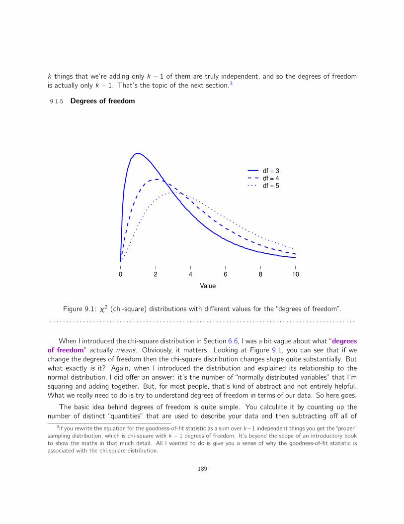
k things that we’re adding only k ´ 1 of them are truly independent, and so the degrees of freedomis actually only k ´ 1. That’s the topic of the next section.3

9.1.5 Degrees of freedom

0 2 4 6 8 10

Value

df = 3

df = 4

df = 5

Figure 9.1: χ2 (chi-square) distributions with different values for the “degrees of freedom”.

. . . . . . . . . . . . . . . . . . . . . . . . . . . . . . . . . . . . . . . . . . . . . . . . . . . . . . . . . . . . . . . . . . . . . . . . . . . . . . . . . . . . . . . . . . . .

When I introduced the chi-square distribution in Section 6.6, I was a bit vague about what “degreesof freedom” actually means. Obviously, it matters. Looking at Figure 9.1, you can see that if wechange the degrees of freedom then the chi-square distribution changes shape quite substantially. Butwhat exactly is it? Again, when I introduced the distribution and explained its relationship to thenormal distribution, I did offer an answer: it’s the number of “normally distributed variables” that I’msquaring and adding together. But, for most people, that’s kind of abstract and not entirely helpful.What we really need to do is try to understand degrees of freedom in terms of our data. So here goes.

The basic idea behind degrees of freedom is quite simple. You calculate it by counting up thenumber of distinct “quantities” that are used to describe your data and then subtracting off all of

3If you rewrite the equation for the goodness-of-fit statistic as a sum over k´1 independent things you get the “proper”sampling distribution, which is chi-square with k ´ 1 degrees of freedom. It’s beyond the scope of an introductory bookto show the maths in that much detail. All I wanted to do is give you a sense of why the goodness-of-fit statistic isassociated with the chi-square distribution.

- 189 -

the “constraints” that those data must satisfy.4 This is a bit vague, so let’s use our cards data asa concrete example. We describe our data using four numbers, O1, O2, O3 and O4 correspondingto the observed frequencies of the four different categories (hearts, clubs, diamonds, spades). Thesefour numbers are the random outcomes of our experiment. But my experiment actually has a fixedconstraint built into it: the sample size N.5 That is, if we know how many people chose hearts,how many chose diamonds and how many chose clubs, then we’d be able to figure out exactly howmany chose spades. In other words, although our data are described using four numbers, they onlyactually correspond to 4 ´ 1 “ 3 degrees of freedom. A slightly different way of thinking about it isto notice that there are four probabilities that we’re interested in (again, corresponding to the fourdifferent categories), but these probabilities must sum to one, which imposes a constraint. Thereforethe degrees of freedom is 4´1 “ 3. Regardless of whether you want to think about it in terms of theobserved frequencies or in terms of the probabilities, the answer is the same. In general, when runningthe χ2 (chi-square) goodness-of-fit test for an experiment involving k groups, then the degrees offreedom will be k ´ 1.

9.1.6 Testing the null hypothesis

The final step in the process of constructing our hypothesis test is to figure out what the rejectionregion is. That is, what values of χ2 would lead us to reject the null hypothesis. As we saw earlier,large values of χ2 imply that the null hypothesis has done a poor job of predicting the data from ourexperiment, whereas small values of χ2 imply that it’s actually done pretty well. Therefore, a prettysensible strategy would be to say there is some critical value such that if χ2 is bigger than the criticalvalue we reject the null, but if χ2 is smaller than this value we retain the null. In other words, to usethe language we introduced in Chapter 8 the chi-square goodness-of-fit test is always a one-sidedtest. Right, so all we have to do is figure out what this critical value is. And it’s pretty straightforward.If we want our test to have significance level of α “ .05 (that is, we are willing to tolerate a Type Ierror rate of 5%), then we have to choose our critical value so that there is only a 5% chance thatχ2 could get to be that big if the null hypothesis is true. This is illustrated in Figure 9.2.

Ah but, I hear you ask, how do I find the critical value of a chi-square distribution with k ´ 1

degrees of freedom? Many many years ago when I first took a psychology statistics class we used tolook up these critical values in a book of critical value tables, like the one in Figure 9.3. Looking atthis Figure, we can see that the critical value for a χ2 distribution with 3 degrees of freedom, and

4I feel obliged to point out that this is an over-simplification. It works nicely for quite a few situations, but every nowand then we’ll come across degrees of freedom values that aren’t whole numbers. Don’t let this worry you too much;when you come across this just remind yourself that “degrees of freedom” is actually a bit of a messy concept, and thatthe nice simple story that I’m telling you here isn’t the whole story. For an introductory class it’s usually best to stick tothe simple story, but I figure it’s best to warn you to expect this simple story to fall apart. If I didn’t give you this warningyou might start getting confused when you see df “ 3.4 or something, (incorrectly) thinking that you had misunderstoodsomething that I’ve taught you rather than (correctly) realising that there’s something that I haven’t told you.

5In practice, the sample size isn’t always fixed. For example, we might run the experiment over a fixed period oftime and the number of people participating depends on how many people show up. That doesn’t matter for the currentpurposes.

- 190 -

0 2 4 6 8 10 12 14

Value of the GOF Statistic

The critical value is 7.81

The observed GOF value is 8.44

7.82 7.82

8.44

7.82

8.44

Figure 9.2: Illustration of how the hypothesis testing works for the χ2 (chi-square) goodness-of-fittest.

. . . . . . . . . . . . . . . . . . . . . . . . . . . . . . . . . . . . . . . . . . . . . . . . . . . . . . . . . . . . . . . . . . . . . . . . . . . . . . . . . . . . . . . . . . . .

p=0.05 is 7.815.

So, if our calculated χ2 statistic is bigger than the critical value of 7.815, then we can reject thenull hypothesis (remember that the null hypothesis, H0, is that all four suits are chosen with equalprobability). Since we actually already calculated that before (i.e., χ2 “ 8.44) we can reject the nullhypothesis. And that’s it, basically. You now know “Pearson’s χ2 test for the goodness-of-fit”. Luckyyou.

9.1.7 Doing the test in JASP

Not surprisingly, JASP provides an analysis that will do these calculations for you. From the main‘Analyses’ toolbar select ‘Frequencies’ - ‘Multinomial Test’. Then in the analysis window that appearsmove the variable you want to analyse (choice_1 across into the ‘Factor’ box. Also, click on the‘Descriptives’ check box so that you see the expected counts in the results table. When you havedone all this, you should see the analysis results in JASP as in Figure 9.4. No surprise then that JASPprovides the same expected counts and statistics that we calculated by hand above, with a χ2 valueof 8.44 with 3 d.f. and p=0.038. Note that we don’t need to look up a critical p-value threshold value

- 191 -

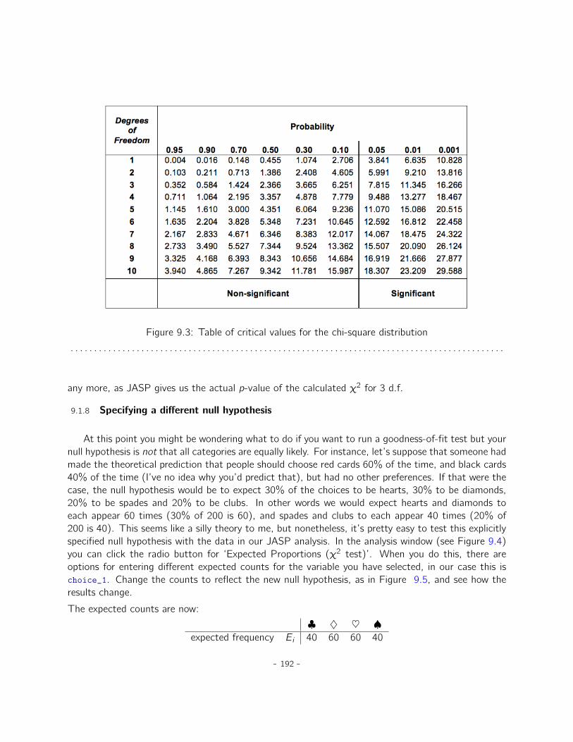
Figure 9.3: Table of critical values for the chi-square distribution

. . . . . . . . . . . . . . . . . . . . . . . . . . . . . . . . . . . . . . . . . . . . . . . . . . . . . . . . . . . . . . . . . . . . . . . . . . . . . . . . . . . . . . . . . . . .

any more, as JASP gives us the actual p-value of the calculated χ2 for 3 d.f.

9.1.8 Specifying a different null hypothesis

At this point you might be wondering what to do if you want to run a goodness-of-fit test but yournull hypothesis is not that all categories are equally likely. For instance, let’s suppose that someone hadmade the theoretical prediction that people should choose red cards 60% of the time, and black cards40% of the time (I’ve no idea why you’d predict that), but had no other preferences. If that were thecase, the null hypothesis would be to expect 30% of the choices to be hearts, 30% to be diamonds,20% to be spades and 20% to be clubs. In other words we would expect hearts and diamonds toeach appear 60 times (30% of 200 is 60), and spades and clubs to each appear 40 times (20% of200 is 40). This seems like a silly theory to me, but nonetheless, it’s pretty easy to test this explicitlyspecified null hypothesis with the data in our JASP analysis. In the analysis window (see Figure 9.4)you can click the radio button for ‘Expected Proportions (χ2 test)’. When you do this, there areoptions for entering different expected counts for the variable you have selected, in our case this ischoice_1. Change the counts to reflect the new null hypothesis, as in Figure 9.5, and see how theresults change.

The expected counts are now:

♣ ♦ ♥ ♠expected frequency Ei 40 60 60 40

- 192 -

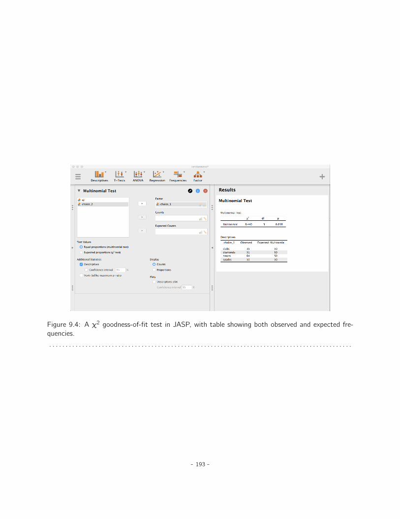
Figure 9.4: A χ2 goodness-of-fit test in JASP, with table showing both observed and expected fre-quencies.

. . . . . . . . . . . . . . . . . . . . . . . . . . . . . . . . . . . . . . . . . . . . . . . . . . . . . . . . . . . . . . . . . . . . . . . . . . . . . . . . . . . . . . . . . . . .

- 193 -

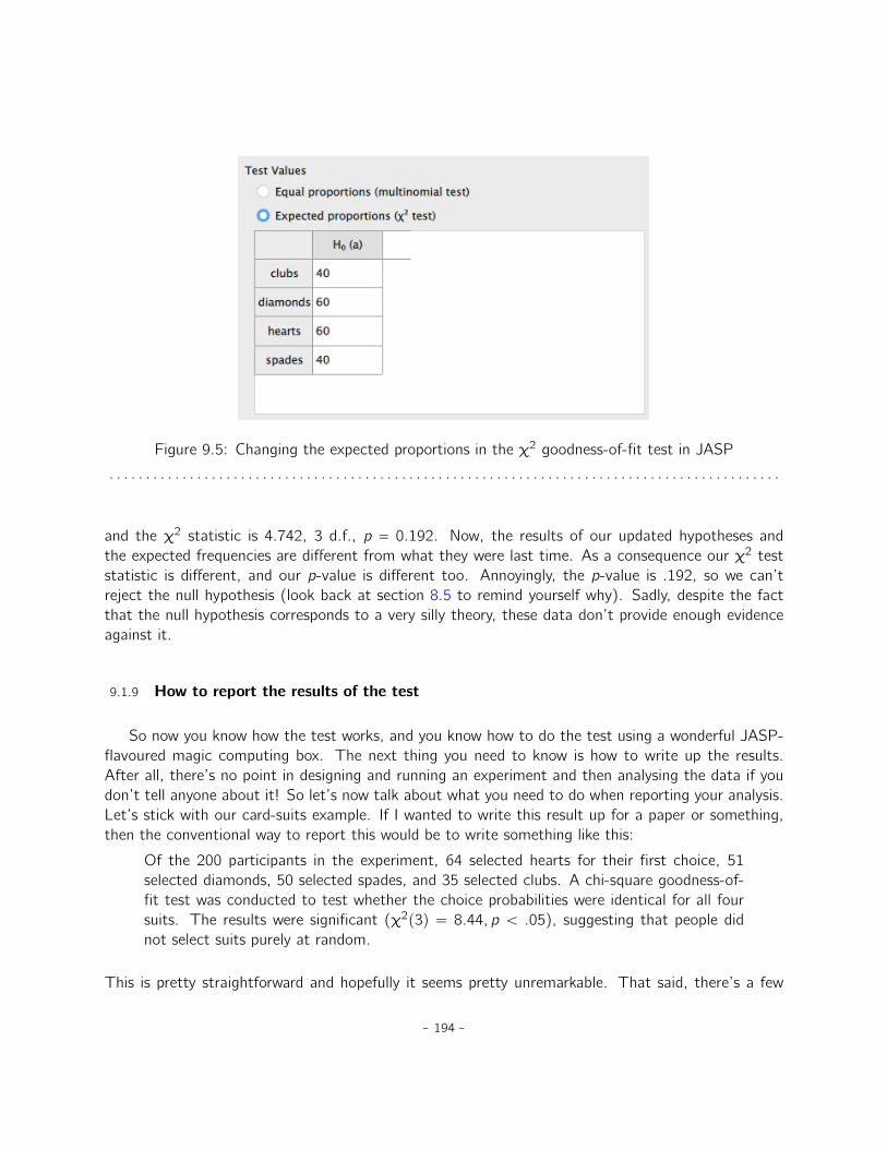
Figure 9.5: Changing the expected proportions in the χ2 goodness-of-fit test in JASP

. . . . . . . . . . . . . . . . . . . . . . . . . . . . . . . . . . . . . . . . . . . . . . . . . . . . . . . . . . . . . . . . . . . . . . . . . . . . . . . . . . . . . . . . . . . .

and the χ2 statistic is 4.742, 3 d.f., p = 0.192. Now, the results of our updated hypotheses andthe expected frequencies are different from what they were last time. As a consequence our χ2 teststatistic is different, and our p-value is different too. Annoyingly, the p-value is .192, so we can’treject the null hypothesis (look back at section 8.5 to remind yourself why). Sadly, despite the factthat the null hypothesis corresponds to a very silly theory, these data don’t provide enough evidenceagainst it.

9.1.9 How to report the results of the test

So now you know how the test works, and you know how to do the test using a wonderful JASP-flavoured magic computing box. The next thing you need to know is how to write up the results.After all, there’s no point in designing and running an experiment and then analysing the data if youdon’t tell anyone about it! So let’s now talk about what you need to do when reporting your analysis.Let’s stick with our card-suits example. If I wanted to write this result up for a paper or something,then the conventional way to report this would be to write something like this:

Of the 200 participants in the experiment, 64 selected hearts for their first choice, 51selected diamonds, 50 selected spades, and 35 selected clubs. A chi-square goodness-of-fit test was conducted to test whether the choice probabilities were identical for all foursuits. The results were significant (χ2p3q “ 8.44, p ă .05), suggesting that people didnot select suits purely at random.

This is pretty straightforward and hopefully it seems pretty unremarkable. That said, there’s a few

- 194 -

things that you should note about this description:

• The statistical test is preceded by the descriptive statistics. That is, I told the reader somethingabout what the data look like before going on to do the test. In general, this is good practice.Always remember that your reader doesn’t know your data anywhere near as well as you do. So,unless you describe it to them properly, the statistical tests won’t make any sense to them andthey’ll get frustrated and cry.

• The description tells you what the null hypothesis being tested is. To be honest, writers don’talways do this but it’s often a good idea in those situations where some ambiguity exists, orwhen you can’t rely on your readership being intimately familiar with the statistical tools thatyou’re using. Quite often the reader might not know (or remember) all the details of the testthat your using, so it’s a kind of politeness to “remind” them! As far as the goodness-of-fittest goes, you can usually rely on a scientific audience knowing how it works (since it’s coveredin most intro stats classes). However, it’s still a good idea to be explicit about stating thenull hypothesis (briefly!) because the null hypothesis can be different depending on what you’reusing the test for. For instance, in the cards example my null hypothesis was that all the foursuit probabilities were identical (i.e., P1 “ P2 “ P3 “ P4 “ 0.25), but there’s nothing specialabout that hypothesis. I could just as easily have tested the null hypothesis that P1 “ 0.7 andP2 “ P3 “ P4 “ 0.1 using a goodness-of-fit test. So it’s helpful to the reader if you explain tothem what your null hypothesis was. Also, notice that I described the null hypothesis in words,not in maths. That’s perfectly acceptable. You can describe it in maths if you like, but sincemost readers find words easier to read than symbols, most writers tend to describe the null usingwords if they can.

• A “stat block” is included. When reporting the results of the test itself, I didn’t just say that theresult was significant, I included a “stat block” (i.e., the dense mathematical-looking part in theparentheses) which reports all the “key” statistical information. For the chi-square goodness-of-fit test, the information that gets reported is the test statistic (that the goodness-of-fit statisticwas 8.44), the information about the distribution used in the test (χ2 with 3 degrees of freedomwhich is usually shortened to χ2p3q), and then the information about whether the result wassignificant (in this case p ă .05). The particular information that needs to go into the stat blockis different for every test, and so each time I introduce a new test I’ll show you what the statblock should look like.6 However the general principle is that you should always provide enoughinformation so that the reader could check the test results themselves if they really wanted to.

• The results are interpreted. In addition to indicating that the result was significant, I providedan interpretation of the result (i.e., that people didn’t choose randomly). This is also a kindnessto the reader, because it tells them something about what they should believe about what’s

6Well, sort of. The conventions for how statistics should be reported tend to differ somewhat from discipline todiscipline. I’ve tended to stick with how things are done in psychology, since that’s what I do. But the general principleof providing enough information to the reader to allow them to check your results is pretty universal, I think.

- 195 -

going on in your data. If you don’t include something like this, it’s really hard for your reader tounderstand what’s going on.7

As with everything else, your overriding concern should be that you explain things to your reader.Always remember that the point of reporting your results is to communicate to another human being.I cannot tell you just how many times I’ve seen the results section of a report or a thesis or even ascientific article that is just gibberish, because the writer has focused solely on making sure they’veincluded all the numbers and forgotten to actually communicate with the human reader.

9.1.10 A comment on statistical notation

Satan delights equally in statistics and in quoting scripture

– H.G. Wells

If you’ve been reading very closely, and are as much of a mathematical pedant as I am, there is onething about the way I wrote up the chi-square test in the last section that might be bugging you alittle bit. There’s something that feels a bit wrong with writing “χ2p3q “ 8.44”, you might be thinking.After all, it’s the goodness-of-fit statistic that is equal to 8.44, so shouldn’t I have written X2 “ 8.44

or maybe GOF“ 8.44? This seems to be conflating the sampling distribution (i.e., χ2 with df “ 3)with the test statistic (i.e., X2). Odds are you figured it was a typo, since χ and X look pretty similar.Oddly, it’s not. Writing χ2p3q “ 8.44 is essentially a highly condensed way of writing “the samplingdistribution of the test statistic is χ2p3q, and the value of the test statistic is 8.44”.

In one sense, this is kind of silly. There are lots of different test statistics out there that turn outto have a chi-square sampling distribution. The X2 statistic that we’ve used for our goodness-of-fittest is only one of many (albeit one of the most commonly encountered ones). In a sensible, perfectlyorganised world we’d always have a separate name for the test statistic and the sampling distribution.That way, the stat block itself would tell you exactly what it was that the researcher had calculated.Sometimes this happens. For instance, the test statistic used in the Pearson goodness-of-fit test iswritten X2, but there’s a closely related test known as the G-test8 (Sokal and Rohlf 1994), in whichthe test statistic is written as G. As it happens, the Pearson goodness-of-fit test and the G-test bothtest the same null hypothesis, and the sampling distribution is exactly the same (i.e., chi-square withk ´ 1 degrees of freedom). If I’d done a G-test for the cards data rather than a goodness-of-fit test,

7To some people, this advice might sound odd, or at least in conflict with the “usual” advice on how to write atechnical report. Very typically, students are told that the “results” section of a report is for describing the data andreporting statistical analysis, and the “discussion” section is for providing interpretation. That’s true as far as it goes,but I think people often interpret it way too literally. The way I usually approach it is to provide a quick and simpleinterpretation of the data in the results section, so that my reader understands what the data are telling us. Then, inthe discussion, I try to tell a bigger story about how my results fit with the rest of the scientific literature. In short,don’t let the “interpretation goes in the discussion” advice turn your results section into incomprehensible garbage. Beingunderstood by your reader is much more important.

8Complicating matters, the G-test is a special case of a whole class of tests that are known as likelihood ratio tests.I don’t cover LRTs in this book, but they are quite handy things to know about.

- 196 -

then I’d have ended up with a test statistic of G “ 8.65, which is slightly different from the X2 “ 8.44

value that I got earlier and which produces a slightly smaller p-value of p “ .034. Suppose that theconvention was to report the test statistic, then the sampling distribution, and then the p-value. Ifthat were true, then these two situations would produce different stat blocks: my original result wouldbe written X2 “ 8.44, χ2p3q, p “ .038, whereas the new version using the G-test would be writtenas G “ 8.65, χ2p3q, p “ .034. However, using the condensed reporting standard, the original resultis written χ2p3q “ 8.44, p “ .038, and the new one is written χ2p3q “ 8.65, p “ .034, and so it’sactually unclear which test I actually ran.

So why don’t we live in a world in which the contents of the stat block uniquely specifies whattests were ran? The deep reason is that life is messy. We (as users of statistical tools) want itto be nice and neat and organised. We want it to be designed, as if it were a product, but that’snot how life works. Statistics is an intellectual discipline just as much as any other one, and assuch it’s a massively distributed, partly-collaborative and partly-competitive project that no-one reallyunderstands completely. The things that you and I use as data analysis tools weren’t created by anAct of the Gods of Statistics. They were invented by lots of different people, published as papers inacademic journals, implemented, corrected and modified by lots of other people, and then explainedto students in textbooks by someone else. As a consequence, there’s a lot of test statistics thatdon’t even have names, and as a consequence they’re just given the same name as the correspondingsampling distribution. As we’ll see later, any test statistic that follows a χ2 distribution is commonlycalled a “chi-square statistic”, anything that follows a t-distribution is called a “t-statistic”, and so on.But, as the χ2 versus G example illustrates, two different things with the same sampling distributionare still, well, different.

As a consequence, it’s sometimes a good idea to be clear about what the actual test was thatyou ran, especially if you’re doing something unusual. If you just say “chi-square test” it’s not actuallyclear what test you’re talking about. Although, since the two most common chi-square tests are thegoodness-of-fit test and the independence test (Section 9.2), most readers with stats training canprobably guess. Nevertheless, it’s something to be aware of.

- 197 -

9.2

The χ2 test of independence (or association)

GUARDBOT 1: Halt!GUARDBOT 2: Be you robot or human?LEELA: Robot...we be.FRY: Uh, yup! Just two robots out roboting it up! Eh?GUARDBOT 1: Administer the test.GUARDBOT 2: Which of the following would you most prefer?

A: A puppy, B: A pretty flower from your sweetie,or C: A large properly-formatted data file?

GUARDBOT 1: Choose!

– Futurama, “Fear of a Bot Planet”

The other day I was watching an animated documentary examining the quaint customs of the nativesof the planet Chapek 9. Apparently, in order to gain access to their capital city a visitor must prove thatthey’re a robot, not a human. In order to determine whether or not a visitor is human, the natives askwhether the visitor prefers puppies, flowers, or large, properly formatted data files. “Pretty clever,” Ithought to myself “but what if humans and robots have the same preferences? That probably wouldn’tbe a very good test then, would it?” As it happens, I got my hands on the testing data that the civilauthorities of Chapek 9 used to check this. It turns out that what they did was very simple. Theyfound a bunch of robots and a bunch of humans and asked them what they preferred. I saved theirdata in a file called chapek9.csv, which we can now load into JASP. As well as the ID variable thatidentifies individual people, there are two nominal text variables, species and choice. In total thereare 180 entries in the data set, one for each person (counting both robots and humans as “people”)who was asked to make a choice. Specifically, there are 93 humans and 87 robots, and overwhelminglythe preferred choice is the data file. You can check this yourself by asking JASP for Frequency Tables,under the ‘Descriptives’ - ‘Descriptive Statistics’ button. However, this summary does not addressthe question we’re interested in. To do that, we need a more detailed description of the data. Whatwe want to do is look at the choices broken down by species. That is, we need to cross-tabulate thedata. In JASP we do this using the ‘Frequencies’ - ‘Contingency Tables’ button, moving species intothe ‘Columns’ box and choice into the ‘Rows’ box. This procedure should produce a table similar tothis:

Robot Human TotalPuppy 13 15 28Flower 30 13 43Data 44 65 109Total 87 93 180

- 198 -

From this, it’s quite clear that the vast majority of the humans chose the data file, whereas therobots tended to be a lot more even in their preferences. Leaving aside the question of why thehumans might be more likely to choose the data file for the moment (which does seem quite odd,admittedly), our first order of business is to determine if the discrepancy between human choices androbot choices in the data set is statistically significant.

9.2.1 Constructing our hypothesis test

How do we analyse this data? Specifically, since my research hypothesis is that “humans and robotsanswer the question in different ways”, how can I construct a test of the null hypothesis that “humansand robots answer the question the same way”? As before, we begin by establishing some notation todescribe the data:

Robot Human TotalPuppy O11 O12 R1

Flower O21 O22 R2

Data O31 O32 R3

Total C1 C2 N

In this notation we say that Oi j is a count (observed frequency) of the number of respondents thatare of species j (robots or human) who gave answer i (puppy, flower or data) when asked to make achoice. The total number of observations is written N, as usual. Finally, I’ve used Ri to denote therow totals (e.g., R1 is the total number of people who chose the flower), and Cj to denote the columntotals (e.g., C1 is the total number of robots).9

So now let’s think about what the null hypothesis says. If robots and humans are responding inthe same way to the question, it means that the probability that “a robot says puppy” is the sameas the probability that “a human says puppy”, and so on for the other two possibilities. So, if we usePi j to denote “the probability that a member of species j gives response i ” then our null hypothesis isthat:

H0: All of the following are true:P11 “ P12 (same probability of saying “puppy”),P21 “ P22 (same probability of saying “flower”), andP31 “ P32 (same probability of saying “data”).

And actually, since the null hypothesis is claiming that the true choice probabilities don’t depend onthe species of the person making the choice, we can let Pi refer to this probability, e.g., P1 is the true

9A technical note. The way I’ve described the test pretends that the column totals are fixed (i.e., the researcherintended to survey 87 robots and 93 humans) and the row totals are random (i.e., it just turned out that 28 peoplechose the puppy). To use the terminology from my mathematical statistics textbook (Hogg, McKean, and Craig 2005),I should technically refer to this situation as a chi-square test of homogeneity and reserve the term chi-square test ofindependence for the situation where both the row and column totals are random outcomes of the experiment. In theinitial drafts of this book that’s exactly what I did. However, it turns out that these two tests are identical, and so I’vecollapsed them together.

- 199 -

probability of choosing the puppy.

Next, in much the same way that we did with the goodness-of-fit test, what we need to do iscalculate the expected frequencies. That is, for each of the observed counts Oi j , we need to figureout what the null hypothesis would tell us to expect. Let’s denote this expected frequency by Ei j .This time, it’s a little bit trickier. If there are a total of Cj people that belong to species j , and thetrue probability of anyone (regardless of species) choosing option i is Pi , then the expected frequencyis just:

Ei j “ Cj ˆ Pi

Now, this is all very well and good, but we have a problem. Unlike the situation we had with thegoodness-of-fit test, the null hypothesis doesn’t actually specify a particular value for Pi . It’s somethingwe have to estimate (Chapter 7) from the data! Fortunately, this is pretty easy to do. If 28 out of 180people selected the flowers, then a natural estimate for the probability of choosing flowers is 28{180,which is approximately .16. If we phrase this in mathematical terms, what we’re saying is that ourestimate for the probability of choosing option i is just the row total divided by the total sample size:

Pi “RiN

Therefore, our expected frequency can be written as the product (i.e. multiplication) of the row totaland the column total, divided by the total number of observations:10

Ei j “Ri ˆ CjN

Now that we’ve figured out how to calculate the expected frequencies, it’s straightforward to definea test statistic, following the exact same strategy that we used in the goodness-of-fit test. In fact,it’s pretty much the same statistic.

For a contingency table with r rows and c columns, the equation that defines our X2 statistic is

X2 “

rÿ

i“1

cÿ

j“1

pEi j ´Oi jq2

Ei j

The only difference is that I have to include two summation signs (i.e.,ř

) to indicate that we’resumming over both rows and columns.

As before, large values of X2 indicate that the null hypothesis provides a poor description of thedata, whereas small values of X2 suggest that it does a good job of accounting for the data. Therefore,just like last time, we want to reject the null hypothesis if X2 is too large.

Not surprisingly, this statistic is χ2 distributed. All we need to do is figure out how many degreesof freedom are involved, which actually isn’t too hard. As I mentioned before, you can (usually) think

10Technically, Ei j here is an estimate, so I should probably write it Ei j . But since no-one else does, I won’t either.

- 200 -

of the degrees of freedom as being equal to the number of data points that you’re analysing, minusthe number of constraints. A contingency table with r rows and c columns contains a total of r ˆ cobserved frequencies, so that’s the total number of observations. What about the constraints? Here,it’s slightly trickier. The answer is always the same

df “ pr ´ 1qpc ´ 1q

but the explanation for why the degrees of freedom takes this value is different depending on theexperimental design. For the sake of argument, let’s suppose that we had honestly intended to surveyexactly 87 robots and 93 humans (column totals fixed by the experimenter), but left the row totalsfree to vary (row totals are random variables). Let’s think about the constraints that apply here.Well, since we deliberately fixed the column totals by Act of Experimenter, we have c constraints rightthere. But, there’s actually more to it than that. Remember how our null hypothesis had some freeparameters (i.e., we had to estimate the Pi values)? Those matter too. I won’t explain why in thisbook, but every free parameter in the null hypothesis is rather like an additional constraint. So, howmany of those are there? Well, since these probabilities have to sum to 1, there’s only r ´ 1 of these.So our total degrees of freedom is:

df “ (number of observations)´ (number of constraints)“ prcq ´ pc ` pr ´ 1qq

“ rc ´ c ´ r ` 1

“ pr ´ 1qpc ´ 1q

Alternatively, suppose that the only thing that the experimenter fixed was the total sample size N.That is, we quizzed the first 180 people that we saw and it just turned out that 87 were robots and93 were humans. This time around our reasoning would be slightly different, but would still lead usto the same answer. Our null hypothesis still has r ´ 1 free parameters corresponding to the choiceprobabilities, but it now also has c ´ 1 free parameters corresponding to the species probabilities,because we’d also have to estimate the probability that a randomly sampled person turns out to bea robot.11 Finally, since we did actually fix the total number of observations N, that’s one moreconstraint. So, now we have rc observations, and pc ´ 1q ` pr ´ 1q ` 1 constraints. What does thatgive?

df “ (number of observations)´ (number of constraints)“ rc ´ ppc ´ 1q ` pr ´ 1q ` 1q

“ rc ´ c ´ r ` 1

“ pr ´ 1qpc ´ 1q

Amazing.


Okay, now that we know how the test works let’s have a look at how it’s done in JASP. Astempting as it is to lead you through the tedious calculations so that you’re forced to learn it the long

11A problem many of us worry about in real life.

- 201 -

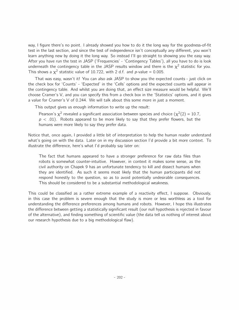
way, I figure there’s no point. I already showed you how to do it the long way for the goodness-of-fittest in the last section, and since the test of independence isn’t conceptually any different, you won’tlearn anything new by doing it the long way. So instead I’ll go straight to showing you the easy way.After you have run the test in JASP (‘Frequencies’ - ‘Contingency Tables’), all you have to do is lookunderneath the contingency table in the JASP results window and there is the χ2 statistic for you.This shows a χ2 statistic value of 10.722, with 2 d.f. and p-value = 0.005.

That was easy, wasn’t it! You can also ask JASP to show you the expected counts - just click onthe check box for ‘Counts’ - ‘Expected’ in the ‘Cells’ options and the expected counts will appear inthe contingency table. And whilst you are doing that, an effect size measure would be helpful. We’llchoose Cramer’s V, and you can specify this from a check box in the ‘Statistics’ options, and it givesa value for Cramer’s V of 0.244. We will talk about this some more in just a moment.

This output gives us enough information to write up the result:

Pearson’s χ2 revealed a significant association between species and choice (χ2(2) = 10.7,p ă .01). Robots appeared to be more likely to say that they prefer flowers, but thehumans were more likely to say they prefer data.

Notice that, once again, I provided a little bit of interpretation to help the human reader understandwhat’s going on with the data. Later on in my discussion section I’d provide a bit more context. Toillustrate the difference, here’s what I’d probably say later on:

The fact that humans appeared to have a stronger preference for raw data files thanrobots is somewhat counter-intuitive. However, in context it makes some sense, as thecivil authority on Chapek 9 has an unfortunate tendency to kill and dissect humans whenthey are identified. As such it seems most likely that the human participants did notrespond honestly to the question, so as to avoid potentially undesirable consequences.This should be considered to be a substantial methodological weakness.

This could be classified as a rather extreme example of a reactivity effect, I suppose. Obviously,in this case the problem is severe enough that the study is more or less worthless as a tool forunderstanding the difference preferences among humans and robots. However, I hope this illustratesthe difference between getting a statistically significant result (our null hypothesis is rejected in favourof the alternative), and finding something of scientific value (the data tell us nothing of interest aboutour research hypothesis due to a big methodological flaw).

- 202 -

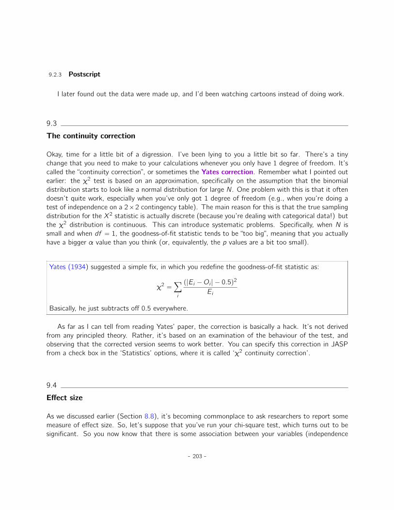
9.2.3 Postscript

I later found out the data were made up, and I’d been watching cartoons instead of doing work.

9.3

The continuity correction

Okay, time for a little bit of a digression. I’ve been lying to you a little bit so far. There’s a tinychange that you need to make to your calculations whenever you only have 1 degree of freedom. It’scalled the “continuity correction”, or sometimes the Yates correction. Remember what I pointed outearlier: the χ2 test is based on an approximation, specifically on the assumption that the binomialdistribution starts to look like a normal distribution for large N. One problem with this is that it oftendoesn’t quite work, especially when you’ve only got 1 degree of freedom (e.g., when you’re doing atest of independence on a 2ˆ2 contingency table). The main reason for this is that the true samplingdistribution for the X2 statistic is actually discrete (because you’re dealing with categorical data!) butthe χ2 distribution is continuous. This can introduce systematic problems. Specifically, when N issmall and when df “ 1, the goodness-of-fit statistic tends to be “too big”, meaning that you actuallyhave a bigger α value than you think (or, equivalently, the p values are a bit too small).

Yates (1934) suggested a simple fix, in which you redefine the goodness-of-fit statistic as:

χ2 “ÿ

i

p|Ei ´Oi | ´ 0.5q2

Ei

Basically, he just subtracts off 0.5 everywhere.

As far as I can tell from reading Yates’ paper, the correction is basically a hack. It’s not derivedfrom any principled theory. Rather, it’s based on an examination of the behaviour of the test, andobserving that the corrected version seems to work better. You can specify this correction in JASPfrom a check box in the ‘Statistics’ options, where it is called ‘χ2 continuity correction’.

9.4

Effect size

As we discussed earlier (Section 8.8), it’s becoming commonplace to ask researchers to report somemeasure of effect size. So, let’s suppose that you’ve run your chi-square test, which turns out to besignificant. So you now know that there is some association between your variables (independence

- 203 -

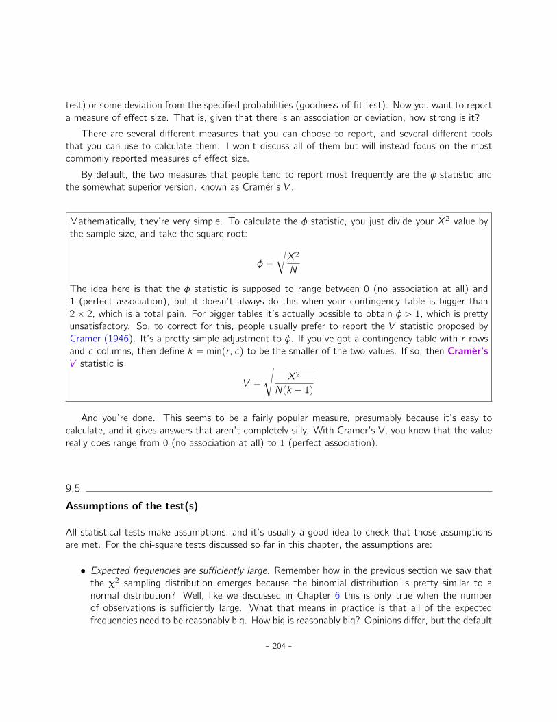
test) or some deviation from the specified probabilities (goodness-of-fit test). Now you want to reporta measure of effect size. That is, given that there is an association or deviation, how strong is it?

There are several different measures that you can choose to report, and several different toolsthat you can use to calculate them. I won’t discuss all of them but will instead focus on the mostcommonly reported measures of effect size.

By default, the two measures that people tend to report most frequently are the φ statistic andthe somewhat superior version, known as Cramér’s V .

Mathematically, they’re very simple. To calculate the φ statistic, you just divide your X2 value bythe sample size, and take the square root:

φ “

c

X2

N

The idea here is that the φ statistic is supposed to range between 0 (no association at all) and1 (perfect association), but it doesn’t always do this when your contingency table is bigger than2ˆ 2, which is a total pain. For bigger tables it’s actually possible to obtain φ ą 1, which is prettyunsatisfactory. So, to correct for this, people usually prefer to report the V statistic proposed byCramer (1946). It’s a pretty simple adjustment to φ. If you’ve got a contingency table with r rowsand c columns, then define k “ minpr, cq to be the smaller of the two values. If so, then Cramér’sV statistic is

V “

d

X2

Npk ´ 1q

And you’re done. This seems to be a fairly popular measure, presumably because it’s easy tocalculate, and it gives answers that aren’t completely silly. With Cramer’s V, you know that the valuereally does range from 0 (no association at all) to 1 (perfect association).

9.5

Assumptions of the test(s)

All statistical tests make assumptions, and it’s usually a good idea to check that those assumptionsare met. For the chi-square tests discussed so far in this chapter, the assumptions are:

• Expected frequencies are sufficiently large. Remember how in the previous section we saw thatthe χ2 sampling distribution emerges because the binomial distribution is pretty similar to anormal distribution? Well, like we discussed in Chapter 6 this is only true when the numberof observations is sufficiently large. What that means in practice is that all of the expectedfrequencies need to be reasonably big. How big is reasonably big? Opinions differ, but the default

- 204 -

assumption seems to be that you generally would like to see all your expected frequencies largerthan about 5, though for larger tables you would probably be okay if at least 80% of the theexpected frequencies are above 5 and none of them are below 1. However, from what I’ve beenable to discover (e.g., Cochran 1954) these seem to have been proposed as rough guidelines,not hard and fast rules, and they seem to be somewhat conservative (Larntz 1978).

• Data are independent of one another. One somewhat hidden assumption of the chi-square testis that you have to genuinely believe that the observations are independent. Here’s what I mean.Suppose I’m interested in proportion of babies born at a particular hospital that are boys. Iwalk around the maternity wards and observe 20 girls and only 10 boys. Seems like a prettyconvincing difference, right? But later on, it turns out that I’d actually walked into the sameward 10 times and in fact I’d only seen 2 girls and 1 boy. Not as convincing, is it? My original 30observations were massively non-independent, and were only in fact equivalent to 3 independentobservations. Obviously this is an extreme (and extremely silly) example, but it illustrates thebasic issue. Non-independence “stuffs things up”. Sometimes it causes you to falsely reject thenull, as the silly hospital example illustrates, but it can go the other way too. To give a slightlyless stupid example, let’s consider what would happen if I’d done the cards experiment slightlydifferently Instead of asking 200 people to try to imagine sampling one card at random, supposeI asked 50 people to select 4 cards. One possibility would be that everyone selects one heart, oneclub, one diamond and one spade (in keeping with the “representativeness heuristic”; Tversky &Kahneman 1974). This is highly non-random behaviour from people, but in this case I would getan observed frequency of 50 for all four suits. For this example the fact that the observationsare non-independent (because the four cards that you pick will be related to each other) actuallyleads to the opposite effect, falsely retaining the null.

If you happen to find yourself in a situation where independence is violated, it may be possible to usethe nonparametric tests, such as the McNemar test or the Cochran test. Similarly, if your expectedcell counts are too small, check out the Fisher exact test. At present, JASP does not implement thesetests, but check back later! For now, we’ll just mention that these tests exist, but describing them isbeyond the scope of this book.

9.6

Summary

The key ideas discussed in this chapter are:

• The χ2 (chi-square) goodness-of-fit test (Section 9.1) is used when you have a table of observedfrequencies of different categories, and the null hypothesis gives you a set of “known” probabilitiesto compare them to.

- 205 -

• The χ2 (chi-square) test of independence (Section 9.2) is used when you have a contingencytable (cross-tabulation) of two categorical variables. The null hypothesis is that there is norelationship or association between the variables.

• Effect size for a contingency table can be measured in several ways (Section 9.4). In particularwe noted the Cramér’s V statistic.

• Both versions of the Pearson test rely on two assumptions: that the expected frequencies are suf-ficiently large, and that the observations are independent (Section 9.5). Various nonparametrictests can be used for certain kinds of violations of independence or count assumptions.

If you’re interested in learning more about categorical data analysis a good first choice would beAgresti (1996) which, as the title suggests, provides an Introduction to Categorical Data Analysis.If the introductory book isn’t enough for you (or can’t solve the problem you’re working on) youcould consider Agresti (2002), Categorical Data Analysis. The latter is a more advanced text, so it’sprobably not wise to jump straight from this book to that one.

- 206 -

10. Comparing two means

In Chapter 9 we covered the situation when your outcome variable is nominal scale and your predictorvariable is also nominal scale. Lots of real world situations have that character, and so you’ll find thatchi-square tests in particular are quite widely used. However, you’re much more likely to find yourselfin a situation where your outcome variable is interval scale or higher, and what you’re interested in iswhether the average value of the outcome variable is higher in one group or another. For instance,a psychologist might want to know if anxiety levels are higher among parents than non-parents, orif working memory capacity is reduced by listening to music (relative to not listening to music). Ina medical context we might want to know if a new drug increases or decreases blood pressure. Anagricultural scientist might want to know whether adding phosphorus to Australian native plants willkill them.1 In all these situations our outcome variable is a fairly continuous, interval or ratio scalevariable, and our predictor is a binary “grouping” variable. In other words, we want to compare themeans of the two groups.

The standard answer to the problem of comparing means is to use a t-test, of which there areseveral varieties depending on exactly what question you want to solve. As a consequence, the majorityof this chapter focuses on different types of t-test: one sample t-tests are discussed in Section 10.2,independent samples t-tests are discussed in Sections 10.3 and 10.4, and paired samples t-tests arediscussed in Section 10.5. We’ll then talk about one sided tests (Section 10.6) and, after that, we’lltalk a bit about Cohen’s d , which is the standard measure of effect size for a t-test (Section 10.7).The later sections of the chapter focus on the assumptions of the t-tests, and possible remedies ifthey are violated. However, before discussing any of these useful things, we’ll start with a discussionof the z-test.

1Informal experimentation in my garden suggests that yes, it does. Australian natives are adapted to low phosphoruslevels relative to everywhere else on Earth, so if you’ve bought a house with a bunch of exotics and you want to plantnatives, keep them separate; nutrients to European plants are poison to Australian ones.

- 207 -

10.1

The one-sample z-test

In this section I’ll describe one of the most useless tests in all of statistics: the z-test. Seriously– this test is almost never used in real life. Its only real purpose is that, when teaching statistics,it’s a very convenient stepping stone along the way towards the t-test, which is probably the most(over)used tool in all statistics.

10.1.1 The inference problem that the test addresses

To introduce the idea behind the z-test, let’s use a simple example. A friend of mine, Dr. Zeppo,grades his introductory statistics class on a curve. Let’s suppose that the average grade in his classis 67.5, and the standard deviation is 9.5. Of his many hundreds of students, it turns out that 20 ofthem also take psychology classes. Out of curiosity, I find myself wondering if the psychology studentstend to get the same grades as everyone else (i.e., mean 67.5) or do they tend to score higher orlower? He emails me the zeppo.csv file, which I use to look at the grades of those students in JASP(stored in the variable x):

50 60 60 64 66 66 67 69 70 74 76 76 77 79 79 79 81 82 82 89

Then I calculate the mean in ‘Descriptives’ - ‘Descriptive Statistics’. The mean value is 72.3.

Hmm. It might be that the psychology students are scoring a bit higher than normal. That samplemean of X “ 72.3 is a fair bit higher than the hypothesised population mean of µ “ 67.5 but, on theother hand, a sample size of N “ 20 isn’t all that big. Maybe it’s pure chance.

To answer the question, it helps to be able to write down what it is that I think I know. Firstly,I know that the sample mean is X “ 72.3. If I’m willing to assume that the psychology studentshave the same standard deviation as the rest of the class then I can say that the population standarddeviation is σ “ 9.5. I’ll also assume that since Dr Zeppo is grading to a curve, the psychology studentgrades are normally distributed.

Next, it helps to be clear about what I want to learn from the data. In this case my researchhypothesis relates to the population mean µ for the psychology student grades, which is unknown.Specifically, I want to know if µ “ 67.5 or not. Given that this is what I know, can we devise ahypothesis test to solve our problem? The data, along with the hypothesised distribution from whichthey are thought to arise, are shown in Figure 10.1. Not entirely obvious what the right answer is, isit? For this, we are going to need some statistics.

- 208 -

Grades

40 50 60 70 80 90

Figure 10.1: The theoretical distribution (solid line) from which the psychology student grades (bars)are supposed to have been generated.

. . . . . . . . . . . . . . . . . . . . . . . . . . . . . . . . . . . . . . . . . . . . . . . . . . . . . . . . . . . . . . . . . . . . . . . . . . . . . . . . . . . . . . . . . . . .

10.1.2 Constructing the hypothesis test

The first step in constructing a hypothesis test is to be clear about what the null and alternativehypotheses are. This isn’t too hard to do. Our null hypothesis, H0, is that the true population meanµ for psychology student grades is 67.5%, and our alternative hypothesis is that the population meanisn’t 67.5%. If we write this in mathematical notation, these hypotheses become:

H0 : µ “ 67.5

H1 : µ ‰ 67.5

though to be honest this notation doesn’t add much to our understanding of the problem, it’s just acompact way of writing down what we’re trying to learn from the data. The null hypotheses H0 andthe alternative hypothesis H1 for our test are both illustrated in Figure 10.2. In addition to providingus with these hypotheses, the scenario outlined above provides us with a fair amount of backgroundknowledge that might be useful. Specifically, there are two special pieces of information that we canadd:

- 209 -

1. The psychology grades are normally distributed.2. The true standard deviation of these scores σ is known to be 9.5.

For the moment, we’ll act as if these are absolutely trustworthy facts. In real life, this kind of absolutelytrustworthy background knowledge doesn’t exist, and so if we want to rely on these facts we’ll justhave make the assumption that these things are true. However, since these assumptions may or maynot be warranted, we might need to check them. For now though, we’ll keep things simple.

µ = µ0

σ = σ0

null hypothesis

value of X

µ ≠ µ0

σ = σ0

alternative hypothesis

value of X

Figure 10.2: Graphical illustration of the null and alternative hypotheses assumed by the one samplez-test (the two sided version, that is). The null and alternative hypotheses both assume that thepopulation distribution is normal, and additionally assumes that the population standard deviation isknown (fixed at some value σ0). The null hypothesis (left) is that the population mean µ is equalto some specified value µ0. The alternative hypothesis is that the population mean differs from thisvalue, µ ‰ µ0.

. . . . . . . . . . . . . . . . . . . . . . . . . . . . . . . . . . . . . . . . . . . . . . . . . . . . . . . . . . . . . . . . . . . . . . . . . . . . . . . . . . . . . . . . . . . .

The next step is to figure out what we would be a good choice for a diagnostic test statistic,something that would help us discriminate between H0 and H1. Given that the hypotheses all referto the population mean µ, you’d feel pretty confident that the sample mean X would be a prettyuseful place to start. What we could do is look at the difference between the sample mean X and thevalue that the null hypothesis predicts for the population mean. In our example that would mean wecalculate X ´ 67.5. More generally, if we let µ0 refer to the value that the null hypothesis claims isour population mean, then we’d want to calculate

X ´ µ0

If this quantity equals or is very close to 0, things are looking good for the null hypothesis. If thisquantity is a long way away from 0, then it’s looking less likely that the null hypothesis is worthretaining. But how far away from zero should it be for us to reject H0?

- 210 -

To figure that out we need to be a bit more sneaky, and we’ll need to rely on those two pieces ofbackground knowledge that I wrote down previously; namely that the raw data are normally distributedand that we know the value of the population standard deviation σ. If the null hypothesis is actuallytrue, and the true mean is µ0, then these facts together mean that we know the complete populationdistribution of the data: a normal distribution with mean µ0 and standard deviation σ. Adopting thenotation from Section 6.5, a statistician might write this as:

X „ Normalpµ0, σ2q

Okay, if that’s true, then what can we say about the distribution of X? Well, as we discussed earlier(see Section 7.3.3), the sampling distribution of the mean X is also normal, and has mean µ. But thestandard deviation of this sampling distribution sepXq, which is called the standard error of the mean,is

sepXq “σ?N

In other words, if the null hypothesis is true then the sampling distribution of the mean can be writtenas follows:

X „ Normalpµ0, sepXqq

Now comes the trick. What we can do is convert the sample mean X into a standard score (Sec-tion 4.5). This is conventionally written as z , but for now I’m going to refer to it as zX . (The reasonfor using this expanded notation is to help you remember that we’re calculating a standardised versionof a sample mean, not a standardised version of a single observation, which is what a z-score usuallyrefers to). When we do so the z-score for our sample mean is

zX “X ´ µ0

sepXq

or, equivalently

zX “X ´ µ0

σ{?N

This z-score is our test statistic. The nice thing about using this as our test statistic is that like allz-scores, it has a standard normal distribution:

zX „ Normalp0, 1q

(again, see Section 4.5 if you’ve forgotten why this is true). In other words, regardless of what scalethe original data are on, the z-statistic itself always has the same interpretation: it’s equal to thenumber of standard errors that separate the observed sample mean X from the population mean µ0

predicted by the null hypothesis. Better yet, regardless of what the population parameters for theraw scores actually are, the 5% critical regions for the z-test are always the same, as illustrated inFigure 10.3. And what this meant, way back in the days where people did all their statistics by hand,is that someone could publish a table like this:

- 211 -

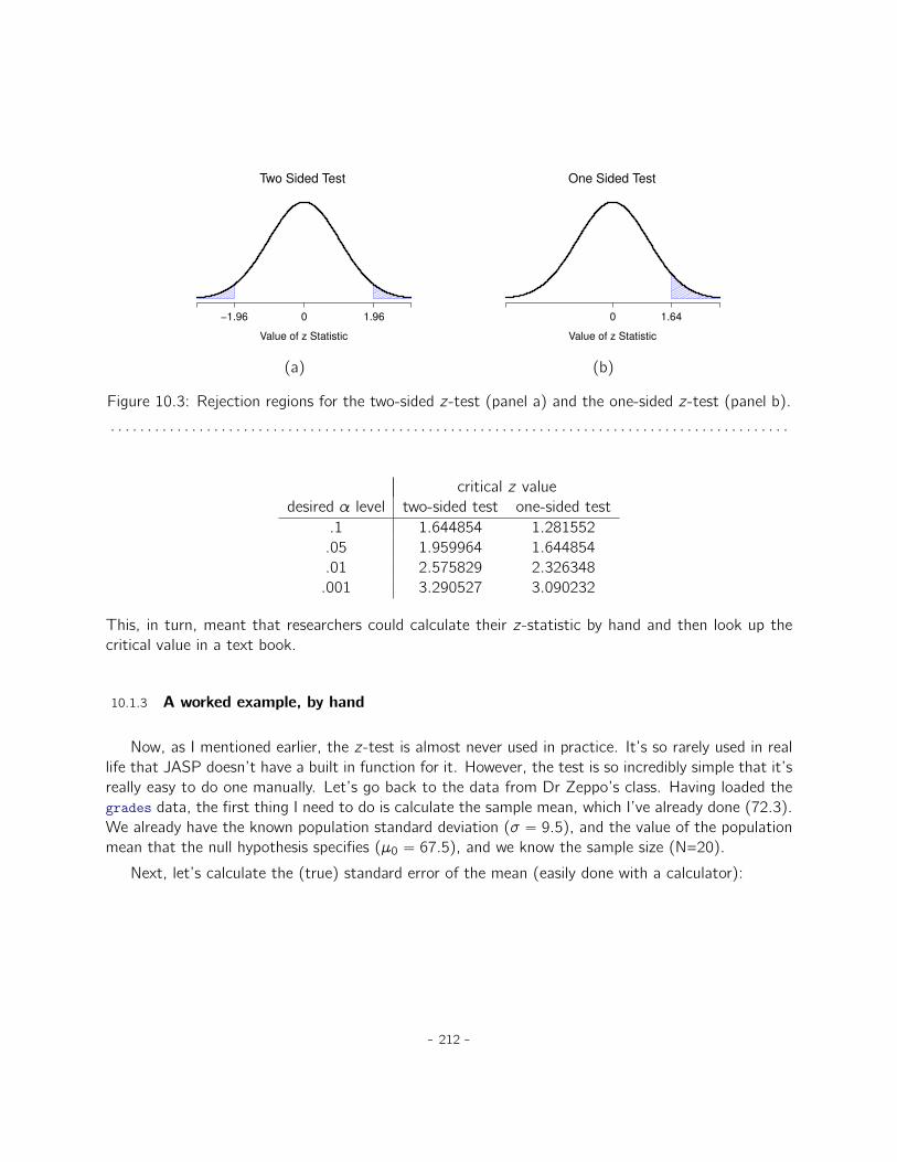
−1.96 0 1.96

Two Sided Test

Value of z Statistic

0 1.64

One Sided Test

Value of z Statistic

(a) (b)

Figure 10.3: Rejection regions for the two-sided z-test (panel a) and the one-sided z-test (panel b).

. . . . . . . . . . . . . . . . . . . . . . . . . . . . . . . . . . . . . . . . . . . . . . . . . . . . . . . . . . . . . . . . . . . . . . . . . . . . . . . . . . . . . . . . . . . .

critical z valuedesired α level two-sided test one-sided test

.1 1.644854 1.281552.05 1.959964 1.644854.01 2.575829 2.326348.001 3.290527 3.090232

This, in turn, meant that researchers could calculate their z-statistic by hand and then look up thecritical value in a text book.

10.1.3 A worked example, by hand

Now, as I mentioned earlier, the z-test is almost never used in practice. It’s so rarely used in reallife that JASP doesn’t have a built in function for it. However, the test is so incredibly simple that it’sreally easy to do one manually. Let’s go back to the data from Dr Zeppo’s class. Having loaded thegrades data, the first thing I need to do is calculate the sample mean, which I’ve already done (72.3).We already have the known population standard deviation (σ “ 9.5), and the value of the populationmean that the null hypothesis specifies (µ0 “ 67.5), and we know the sample size (N=20).

Next, let’s calculate the (true) standard error of the mean (easily done with a calculator):

- 212 -

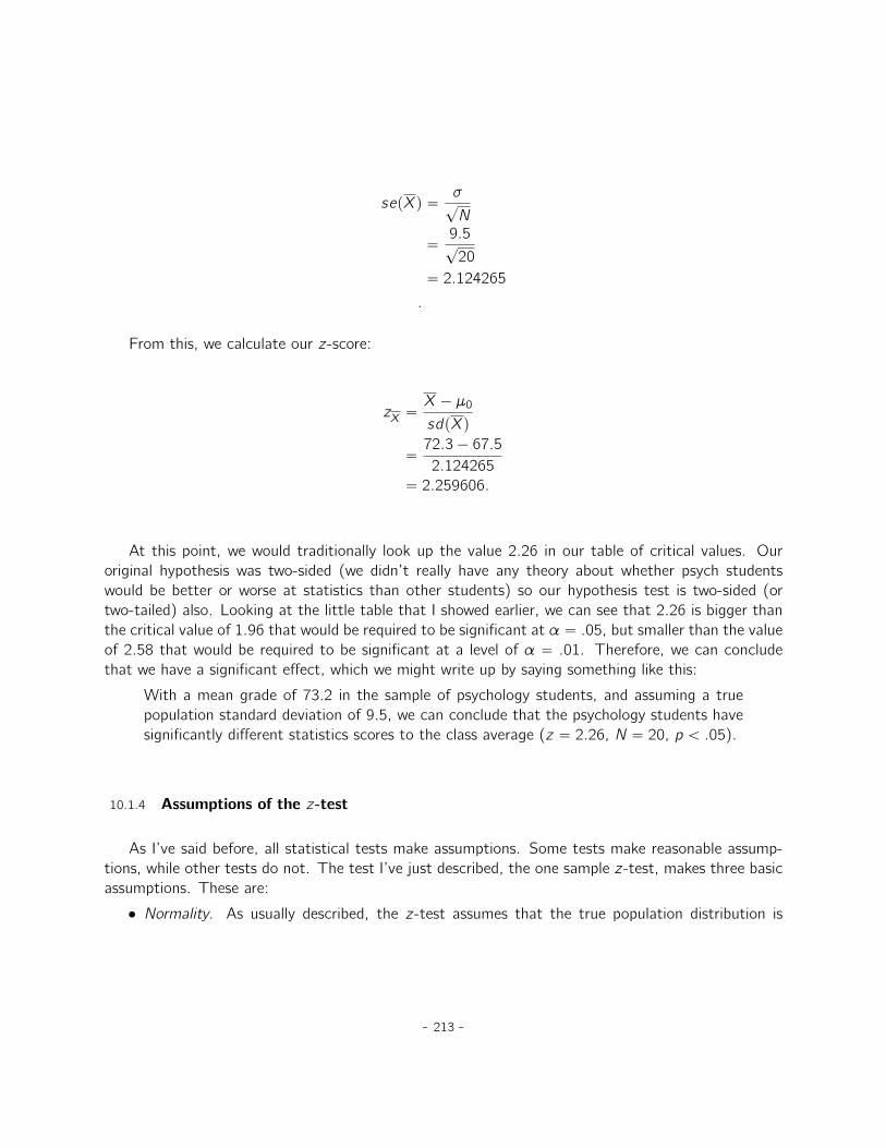
sepXq “σ?N

“9.5?

20

“ 2.124265

.

From this, we calculate our z-score:

zX “X ´ µ0

sdpXq

“72.3´ 67.5

2.124265

“ 2.259606.

At this point, we would traditionally look up the value 2.26 in our table of critical values. Ouroriginal hypothesis was two-sided (we didn’t really have any theory about whether psych studentswould be better or worse at statistics than other students) so our hypothesis test is two-sided (ortwo-tailed) also. Looking at the little table that I showed earlier, we can see that 2.26 is bigger thanthe critical value of 1.96 that would be required to be significant at α “ .05, but smaller than the valueof 2.58 that would be required to be significant at a level of α “ .01. Therefore, we can concludethat we have a significant effect, which we might write up by saying something like this:

With a mean grade of 73.2 in the sample of psychology students, and assuming a truepopulation standard deviation of 9.5, we can conclude that the psychology students havesignificantly different statistics scores to the class average (z “ 2.26, N “ 20, p ă .05).

10.1.4 Assumptions of the z-test

As I’ve said before, all statistical tests make assumptions. Some tests make reasonable assump-tions, while other tests do not. The test I’ve just described, the one sample z-test, makes three basicassumptions. These are:

• Normality. As usually described, the z-test assumes that the true population distribution is

- 213 -

normal.2 This is often a pretty reasonable assumption, and it’s also an assumption that we cancheck if we feel worried about it (see Section 10.8).

• Independence. The second assumption of the test is that the observations in your data set arenot correlated with each other, or related to each other in some funny way. This isn’t as easyto check statistically, it relies a bit on good experimental design. An obvious (and silly) exampleof something that violates this assumption is a data set where you “copy” the same observationover and over again in your data file so that you end up with a massive “sample size”, whichconsists of only one genuine observation. More realistically, you have to ask yourself if it’s reallyplausible to imagine that each observation is a completely random sample from the populationthat you’re interested in. In practice this assumption is never met, but we try our best to designstudies that minimise the problems of correlated data.

• Known standard deviation. The third assumption of the z-test is that the true standard deviationof the population is known to the researcher. This is just silly. In no real world data analysisproblem do you know the standard deviation σ of some population but are completely ignorantabout the mean µ. In other words, this assumption is always wrong.

In view of the stupidity of assuming that σ is known, let’s see if we can live without it. This takes usout of the dreary domain of the z-test, and into the magical kingdom of the t-test!

10.2

The one-sample t-test

After some thought, I decided that it might not be safe to assume that the psychology student gradesnecessarily have the same standard deviation as the other students in Dr Zeppo’s class. After all, ifI’m entertaining the hypothesis that they don’t have the same mean, then why should I believe thatthey absolutely have the same standard deviation? In view of this, I should really stop assuming thatI know the true value of σ. This violates the assumptions of my z-test, so in one sense I’m back tosquare one. However, it’s not like I’m completely bereft of options. After all, I’ve still got my rawdata, and those raw data give me an estimate of the population standard deviation, which is 9.52. Inother words, while I can’t say that I know that σ = 9.5, I can say that σ = 9.52.

Okay, cool. The obvious thing that you might think to do is run a z-test, but using the estimatedstandard deviation of 9.52 instead of relying on my assumption that the true standard deviation is9.5. And you probably wouldn’t be surprised to hear that this would still give us a significant result.

2Actually this is too strong. Strictly speaking the z test only requires that the sampling distribution of the mean benormally distributed. If the population is normal then it necessarily follows that the sampling distribution of the mean isalso normal. However, as we saw when talking about the central limit theorem, it’s quite possible (even commonplace)for the sampling distribution to be normal even if the population distribution itself is non-normal. However, in light of thesheer ridiculousness of the assumption that the true standard deviation is known, there really isn’t much point in goinginto details on this front!

- 214 -

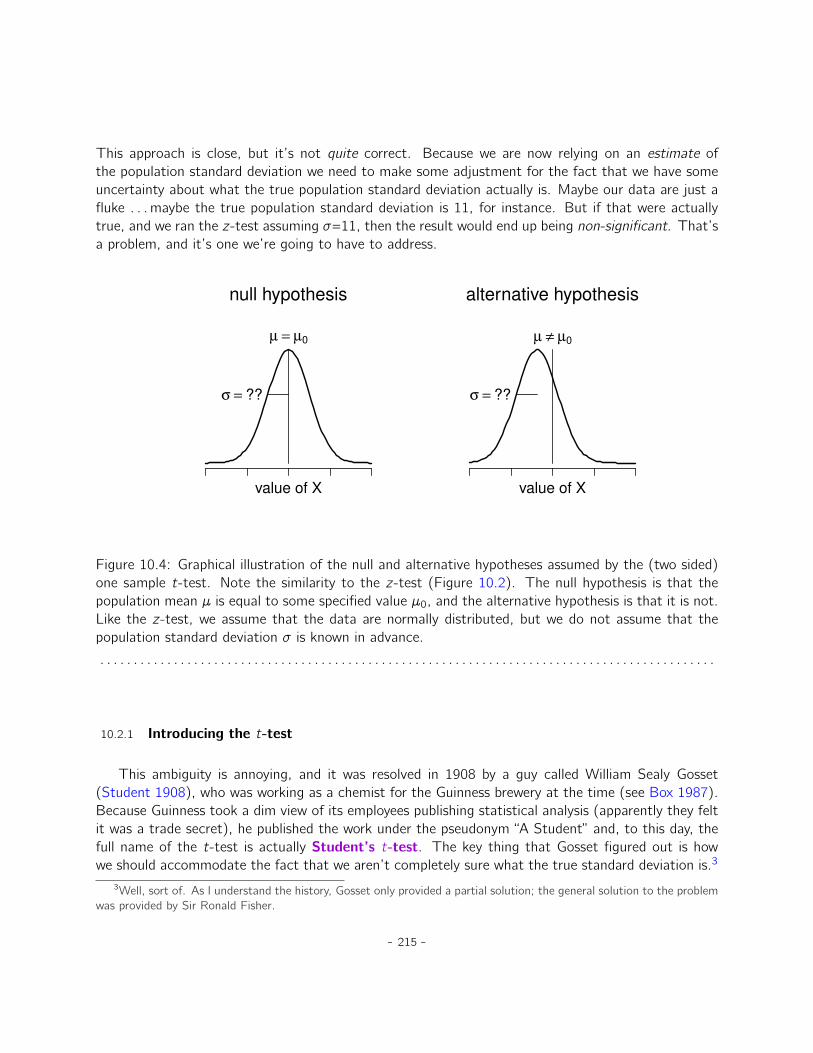
This approach is close, but it’s not quite correct. Because we are now relying on an estimate ofthe population standard deviation we need to make some adjustment for the fact that we have someuncertainty about what the true population standard deviation actually is. Maybe our data are just afluke . . .maybe the true population standard deviation is 11, for instance. But if that were actuallytrue, and we ran the z-test assuming σ=11, then the result would end up being non-significant. That’sa problem, and it’s one we’re going to have to address.

µ = µ0

σ = ??

null hypothesis

value of X

µ ≠ µ0

σ = ??


value of X

Figure 10.4: Graphical illustration of the null and alternative hypotheses assumed by the (two sided)one sample t-test. Note the similarity to the z-test (Figure 10.2). The null hypothesis is that thepopulation mean µ is equal to some specified value µ0, and the alternative hypothesis is that it is not.Like the z-test, we assume that the data are normally distributed, but we do not assume that thepopulation standard deviation σ is known in advance.

. . . . . . . . . . . . . . . . . . . . . . . . . . . . . . . . . . . . . . . . . . . . . . . . . . . . . . . . . . . . . . . . . . . . . . . . . . . . . . . . . . . . . . . . . . . .

10.2.1 Introducing the t-test

This ambiguity is annoying, and it was resolved in 1908 by a guy called William Sealy Gosset(Student 1908), who was working as a chemist for the Guinness brewery at the time (see Box 1987).Because Guinness took a dim view of its employees publishing statistical analysis (apparently they feltit was a trade secret), he published the work under the pseudonym “A Student” and, to this day, thefull name of the t-test is actually Student’s t-test. The key thing that Gosset figured out is howwe should accommodate the fact that we aren’t completely sure what the true standard deviation is.3

3Well, sort of. As I understand the history, Gosset only provided a partial solution; the general solution to the problemwas provided by Sir Ronald Fisher.

- 215 -

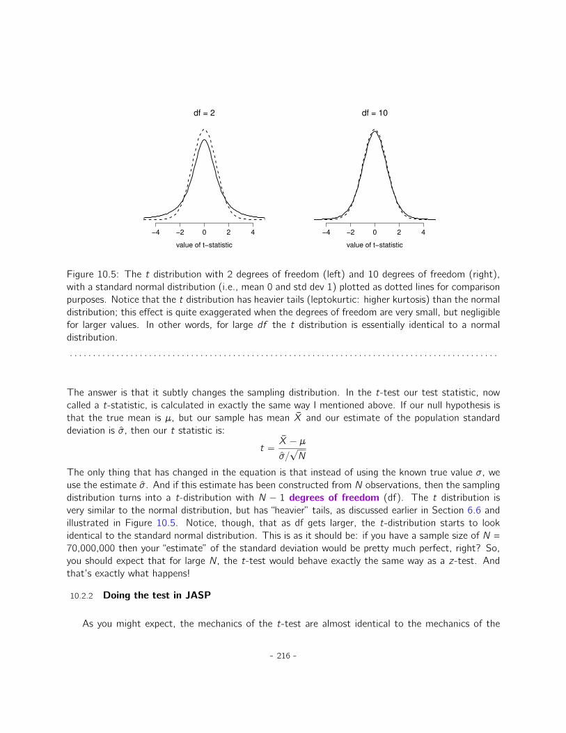
−4 −2 0 2 4

df = 2

value of t−statistic

−4 −2 0 2 4

df = 10

value of t−statistic

Figure 10.5: The t distribution with 2 degrees of freedom (left) and 10 degrees of freedom (right),with a standard normal distribution (i.e., mean 0 and std dev 1) plotted as dotted lines for comparisonpurposes. Notice that the t distribution has heavier tails (leptokurtic: higher kurtosis) than the normaldistribution; this effect is quite exaggerated when the degrees of freedom are very small, but negligiblefor larger values. In other words, for large df the t distribution is essentially identical to a normaldistribution.

. . . . . . . . . . . . . . . . . . . . . . . . . . . . . . . . . . . . . . . . . . . . . . . . . . . . . . . . . . . . . . . . . . . . . . . . . . . . . . . . . . . . . . . . . . . .

The answer is that it subtly changes the sampling distribution. In the t-test our test statistic, nowcalled a t-statistic, is calculated in exactly the same way I mentioned above. If our null hypothesis isthat the true mean is µ, but our sample has mean X and our estimate of the population standarddeviation is σ, then our t statistic is:

t “X ´ µ

σ{?N

The only thing that has changed in the equation is that instead of using the known true value σ, weuse the estimate σ. And if this estimate has been constructed from N observations, then the samplingdistribution turns into a t-distribution with N ´ 1 degrees of freedom (df). The t distribution isvery similar to the normal distribution, but has “heavier” tails, as discussed earlier in Section 6.6 andillustrated in Figure 10.5. Notice, though, that as df gets larger, the t-distribution starts to lookidentical to the standard normal distribution. This is as it should be: if you have a sample size of N =70,000,000 then your “estimate” of the standard deviation would be pretty much perfect, right? So,you should expect that for large N, the t-test would behave exactly the same way as a z-test. Andthat’s exactly what happens!


As you might expect, the mechanics of the t-test are almost identical to the mechanics of the

- 216 -

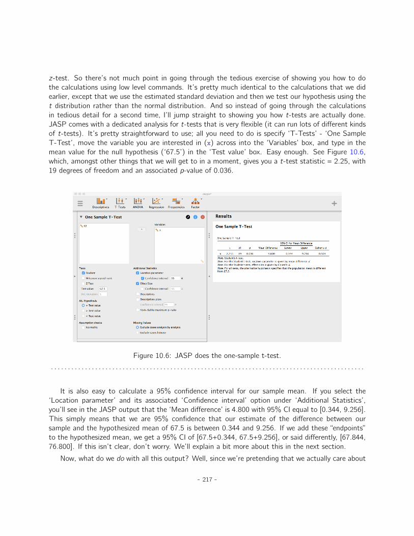
z-test. So there’s not much point in going through the tedious exercise of showing you how to dothe calculations using low level commands. It’s pretty much identical to the calculations that we didearlier, except that we use the estimated standard deviation and then we test our hypothesis using thet distribution rather than the normal distribution. And so instead of going through the calculationsin tedious detail for a second time, I’ll jump straight to showing you how t-tests are actually done.JASP comes with a dedicated analysis for t-tests that is very flexible (it can run lots of different kindsof t-tests). It’s pretty straightforward to use; all you need to do is specify ‘T-Tests’ - ‘One SampleT-Test’, move the variable you are interested in (x) across into the ‘Variables’ box, and type in themean value for the null hypothesis (‘67.5’) in the ‘Test value’ box. Easy enough. See Figure 10.6,which, amongst other things that we will get to in a moment, gives you a t-test statistic = 2.25, with19 degrees of freedom and an associated p-value of 0.036.

Figure 10.6: JASP does the one-sample t-test.

. . . . . . . . . . . . . . . . . . . . . . . . . . . . . . . . . . . . . . . . . . . . . . . . . . . . . . . . . . . . . . . . . . . . . . . . . . . . . . . . . . . . . . . . . . . .

It is also easy to calculate a 95% confidence interval for our sample mean. If you select the‘Location parameter’ and its associated ‘Confidence interval’ option under ‘Additional Statistics’,you’ll see in the JASP output that the ‘Mean difference’ is 4.800 with 95% CI equal to [0.344, 9.256].This simply means that we are 95% confidence that our estimate of the difference between oursample and the hypothesized mean of 67.5 is between 0.344 and 9.256. If we add these “endpoints”to the hypothesized mean, we get a 95% CI of [67.5+0.344, 67.5+9.256], or said differently, [67.844,76.800]. If this isn’t clear, don’t worry. We’ll explain a bit more about this in the next section.

Now, what do we do with all this output? Well, since we’re pretending that we actually care about

- 217 -

my toy example, we’re overjoyed to discover that the result is statistically significant (i.e. p valuebelow .05). We could report the result by saying something like this:

With a mean grade of 72.3, the psychology students scored slightly higher than the averagegrade of 67.5 (tp19q “ 2.25, p ă .05); the 95% confidence interval is 67.8 to 76.8.

where tp19q is shorthand notation for a t-statistic that has 19 degrees of freedom. That said, it’s oftenthe case that people don’t report the confidence interval, or do so using a much more compressedform than I’ve done here. For instance, it’s not uncommon to see the confidence interval included aspart of the stat block, like this:

tp19q “ 2.25, p ă .05, CI95 “ r67.8, 76.8s

With that much jargon crammed into half a line, you know it must be really smart.4

10.2.3 Assumptions of the one sample t-test

Okay, so what assumptions does the one-sample t-test make? Well, since the t-test is basicallya z-test with the assumption of known standard deviation removed, you shouldn’t be surprised to seethat it makes the same assumptions as the z-test, minus the one about the known standard deviation.That is

• Normality. We’re still assuming that the population distribution is normal5, and as noted earlier,there are standard tools that you can use to check to see if this assumption is met (Section 10.8),and other tests you can do in it’s place if this assumption is violated (Section 10.9).

• Independence. Once again, we have to assume that the observations in our sample are gen-erated independently of one another. See the earlier discussion about the z-test for specifics(Section 10.1.4).

Overall, these two assumptions aren’t terribly unreasonable, and as a consequence the one-samplet-test is pretty widely used in practice as a way of comparing a sample mean against a hypothesisedpopulation mean.

4More seriously, I tend to think the reverse is true. I get very suspicious of technical reports that fill their resultssections with nothing except the numbers. It might just be that I’m an arrogant jerk, but I often feel like an authorthat makes no attempt to explain and interpret their analysis to the reader either doesn’t understand it themselves, oris being a bit lazy. Your readers are smart, but not infinitely patient. Don’t annoy them if you can help it.

5A technical comment. In the same way that we can weaken the assumptions of the z-test so that we’re only talkingabout the sampling distribution, we can weaken the t-test assumptions so that we don’t have to assume normality ofthe population. However, for the t-test it’s trickier to do this. As before, we can replace the assumption of populationnormality with an assumption that the sampling distribution of X is normal. However, remember that we’re also relyingon a sample estimate of the standard deviation, and so we also require the sampling distribution of σ to be chi-square.That makes things nastier, and this version is rarely used in practice. Fortunately, if the population distribution is normal,then both of these two assumptions are met.

- 218 -

10.3

The independent samples t-test (Student test)

Although the one sample t-test has its uses, it’s not the most typical example of a t-test6. A muchmore common situation arises when you’ve got two different groups of observations. In psychology,this tends to correspond to two different groups of participants, where each group corresponds to adifferent condition in your study. For each person in the study you measure some outcome variableof interest, and the research question that you’re asking is whether or not the two groups have thesame population mean. This is the situation that the independent samples t-test is designed for.

10.3.1 The data

Suppose we have 33 students taking Dr Harpo’s statistics lectures, and Dr Harpo doesn’t grade toa curve. Actually, Dr Harpo’s grading is a bit of a mystery, so we don’t really know anything aboutwhat the average grade is for the class as a whole. There are two tutors for the class, Anastasiaand Bernadette. There are N1 “ 15 students in Anastasia’s tutorials, and N2 “ 18 in Bernadette’stutorials. The research question I’m interested in is whether Anastasia or Bernadette is a better tutor,or if it doesn’t make much of a difference. Dr Harpo emails me the course grades, in the harpo.csvfile. As usual, I’ll load the file into JASP and have a look at what variables it contains - there are threevariables, ID, grade and tutor. Not surprisingly, the grade variable contains each student’s grade. Thetutor variable is a factor that indicates who each student’s tutor was - either Anastasia or Bernadette.

We can calculate means and standard deviations, using the ‘Descriptives’ - ‘Descriptive Statistics’analysis (being sure to split by tutor). Here’s a nice little summary table:

mean std dev NAnastasia’s students 74.53 9.00 15Bernadette’s students 69.06 5.77 18

To give you a more detailed sense of what’s going on here, I’ve plotted histograms (not in JASP, butusing R) showing the distribution of grades for both tutors (Figure 10.7), as well as a simpler plotshowing the means and corresponding confidence intervals for both groups of students (Figure 10.8).

10.3.2 Introducing the test

The independent samples t-test comes in two different forms, Student’s and Welch’s. Theoriginal Student t-test, which is the one I’ll describe in this section, is the simpler of the two but relieson much more restrictive assumptions than the Welch t-test. Assuming for the moment that you

6Although it is the simplest, which is why I started with it.

- 219 -

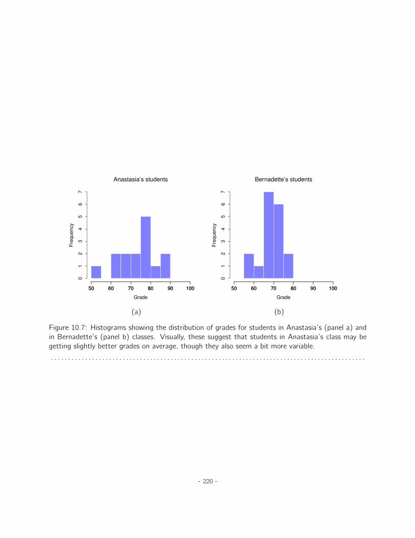
Anastasia’s students

Grade

Fre

qu

en

cy

50 60 70 80 90 100

01

23

45

67

50 60 70 80 90 100

Bernadette’s students

Grade

Fre

qu

en

cy

50 60 70 80 90 100

01

23

45

67

50 60 70 80 90 100

(a) (b)

Figure 10.7: Histograms showing the distribution of grades for students in Anastasia’s (panel a) andin Bernadette’s (panel b) classes. Visually, these suggest that students in Anastasia’s class may begetting slightly better grades on average, though they also seem a bit more variable.

. . . . . . . . . . . . . . . . . . . . . . . . . . . . . . . . . . . . . . . . . . . . . . . . . . . . . . . . . . . . . . . . . . . . . . . . . . . . . . . . . . . . . . . . . . . .

- 220 -

Figure 10.8: The plots show the mean grade for students in Anastasia’s and Bernadette’s tutorials.Error bars depict 95% confidence intervals around the mean. Visually, it does look like there’s a realdifference between the groups, though it’s hard to say for sure.

. . . . . . . . . . . . . . . . . . . . . . . . . . . . . . . . . . . . . . . . . . . . . . . . . . . . . . . . . . . . . . . . . . . . . . . . . . . . . . . . . . . . . . . . . . . .

- 221 -

want to run a two-sided test, the goal is to determine whether two “independent samples” of data aredrawn from populations with the same mean (the null hypothesis) or different means (the alternativehypothesis). When we say “independent” samples, what we really mean here is that there’s no specialrelationship between observations in the two samples. This probably doesn’t make a lot of sense rightnow, but it will be clearer when we come to talk about the paired samples t-test later on. For now,let’s just point out that if we have an experimental design where participants are randomly allocatedto one of two groups, and we want to compare the two groups’ mean performance on some outcomemeasure, then an independent samples t-test (rather than a paired samples t-test) is what we’re after.

Okay, so let’s let µ1 denote the true population mean for group 1 (e.g., Anastasia’s students), andµ2 will be the true population mean for group 2 (e.g., Bernadette’s students),7 and as usual we’ll letX1 and X2 denote the observed sample means for both of these groups. Our null hypothesis statesthat the two population means are identical (µ1 “ µ2) and the alternative to this is that they are not(µ1 ‰ µ2). Written in mathematical notation, this is:

H0 : µ1 “ µ2

H1 : µ1 ‰ µ2

To construct a hypothesis test that handles this scenario we start by noting that if the nullhypothesis is true, then the difference between the population means is exactly zero, µ1 ´ µ2 “ 0.As a consequence, a diagnostic test statistic will be based on the difference between the two samplemeans. Because if the null hypothesis is true, then we’d expect X1 ´ X2 to be pretty close to zero.However, just like we saw with our one-sample tests (i.e., the one-sample z-test and the one-samplet-test) we have to be precise about exactly how close to zero this difference should be. And thesolution to the problem is more or less the same one. We calculate a standard error estimate (SE),just like last time, and then divide the difference between means by this estimate. So our t-statisticwill be of the form:

t “X1 ´ X2

SEWe just need to figure out what this standard error estimate actually is. This is a bit trickier than wasthe case for either of the two tests we’ve looked at so far, so we need to go through it a lot more

7A funny question almost always pops up at this point: what the heck is the population being referred to in thiscase? Is it the set of students actually taking Dr Harpo’s class (all 33 of them)? The set of people who might takethe class (an unknown number of them)? Or something else? Does it matter which of these we pick? It’s traditionalin an introductory behavioural stats class to mumble a lot at this point, but since I get asked this question every yearby my students, I’ll give a brief answer. Technically yes, it does matter. If you change your definition of what the “realworld” population actually is, then the sampling distribution of your observed mean X changes too. The t-test relies onan assumption that the observations are sampled at random from an infinitely large population and, to the extent thatreal life isn’t like that, then the t-test can be wrong. In practice, however, this isn’t usually a big deal. Even though theassumption is almost always wrong, it doesn’t lead to a lot of pathological behaviour from the test, so we tend to justignore it.

- 222 -

µ

null hypothesis

value of X

µ1 µ2


value of X

Figure 10.9: Graphical illustration of the null and alternative hypotheses assumed by the Student t-test.The null hypothesis assumes that both groups have the same mean µ, whereas the alternative assumesthat they have different means µ1 and µ2. Notice that it is assumed that the population distributionsare normal, and that, although the alternative hypothesis allows the group to have different means, itassumes they have the same standard deviation.

. . . . . . . . . . . . . . . . . . . . . . . . . . . . . . . . . . . . . . . . . . . . . . . . . . . . . . . . . . . . . . . . . . . . . . . . . . . . . . . . . . . . . . . . . . . .

carefully to understand how it works.

10.3.3 A “pooled estimate” of the standard deviation

In the original “Student t-test”, we make the assumption that the two groups have the samepopulation standard deviation. That is, regardless of whether the population means are the same, weassume that the population standard deviations are identical, σ1 “ σ2. Since we’re assuming that thetwo standard deviations are the same, we drop the subscripts and refer to both of them as σ. Howshould we estimate this? How should we construct a single estimate of a standard deviation whenwe have two samples? The answer is, basically, we average them. Well, sort of. Actually, what wedo is take a weighed average of the variance estimates, which we use as our pooled estimate of thevariance. The weight assigned to each sample is equal to the number of observations in that sample,minus 1.

- 223 -

Mathematically, we can write this as

w1 “ N1 ´ 1

w2 “ N2 ´ 1

Now that we’ve assigned weights to each sample we calculate the pooled estimate of the varianceby taking the weighted average of the two variance estimates, σ2

1 and σ22

σ2p “

w1σ21 ` w2σ

22

w1 ` w2

Finally, we convert the pooled variance estimate to a pooled standard deviation estimate, by takingthe square root.

σp “

d

w1σ21 ` w2σ

22

w1 ` w2

And if you mentally substitute w1 “ N1 ´ 1 and w2 “ N2 ´ 1 into this equation you get a very uglylooking formula. A very ugly formula that actually seems to be the “standard” way of describing thepooled standard deviation estimate. It’s not my favourite way of thinking about pooled standarddeviations, however. I prefer to think about it like this. Our data set actually corresponds to a setof N observations which are sorted into two groups. So let’s use the notation Xik to refer to thegrade received by the i-th student in the k-th tutorial group. That is, X11 is the grade receivedby the first student in Anastasia’s class, X21 is her second student, and so on. And we have twoseparate group means X1 and X2, which we could “generically” refer to using the notation Xk , i.e.,the mean grade for the k-th tutorial group. So far, so good. Now, since every single student fallsinto one of the two tutorials, we can describe their deviation from the group mean as the difference

Xik ´ Xk

So why not just use these deviations (i.e., the extent to which each student’s grade differs fromthe mean grade in their tutorial)? Remember, a variance is just the average of a bunch of squareddeviations, so let’s do that. Mathematically, we could write it like this

ř

ik

`

Xik ´ Xk˘2

N

where the notation “ř

ik ” is a lazy way of saying “calculate a sum by looking at all students in alltutorials”, since each “ ik” corresponds to one student.a But, as we saw in Chapter 7, calculatingthe variance by dividing by N produces a biased estimate of the population variance. And previouslywe needed to divide by N ´ 1 to fix this. However, as I mentioned at the time, the reason whythis bias exists is because the variance estimate relies on the sample mean, and to the extent thatthe sample mean isn’t equal to the population mean it can systematically bias our estimate of thevariance. But this time we’re relying on two sample means! Does this mean that we’ve got more

- 224 -

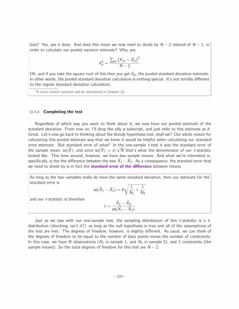
bias? Yes, yes it does. And does this mean we now need to divide by N ´ 2 instead of N ´ 1, inorder to calculate our pooled variance estimate? Why, yes

σ2p “

ř

ik

`

Xik ´ Xk˘2

N ´ 2

Oh, and if you take the square root of this then you get σp, the pooled standard deviation estimate.In other words, the pooled standard deviation calculation is nothing special. It’s not terribly differentto the regular standard deviation calculation.

aA more correct notation will be introduced in Chapter 12.

10.3.4 Completing the test

Regardless of which way you want to think about it, we now have our pooled estimate of thestandard deviation. From now on, I’ll drop the silly p subscript, and just refer to this estimate as σ.Great. Let’s now go back to thinking about the bloody hypothesis test, shall we? Our whole reason forcalculating this pooled estimate was that we knew it would be helpful when calculating our standarderror estimate. But standard error of what? In the one-sample t-test it was the standard error ofthe sample mean, sepXq, and since sepXq “ σ{

?N that’s what the denominator of our t-statistic

looked like. This time around, however, we have two sample means. And what we’re interested in,specifically, is the the difference between the two X1´ X2. As a consequence, the standard error thatwe need to divide by is in fact the standard error of the difference between means.

As long as the two variables really do have the same standard deviation, then our estimate for thestandard error is

sepX1 ´ X2q “ σ

c

1

N1`

1

N2

and our t-statistic is therefore

t “X1 ´ X2

sepX1 ´ X2q

Just as we saw with our one-sample test, the sampling distribution of this t-statistic is a t-distribution (shocking, isn’t it?) as long as the null hypothesis is true and all of the assumptions ofthe test are met. The degrees of freedom, however, is slightly different. As usual, we can think ofthe degrees of freedom to be equal to the number of data points minus the number of constraints.In this case, we have N observations (N1 in sample 1, and N2 in sample 2), and 2 constraints (thesample means). So the total degrees of freedom for this test are N ´ 2.

- 225 -


Not surprisingly, you can run an independent samples t-test easily in JASP. The outcome variablefor our test is the student grade, and the groups are defined in terms of the tutor for each class. Soyou probably won’t be too surprised that all you have to do in JASP is go to the relevant analysis(‘T-Tests’ - ‘Independent Samples T-Test’) and move the grade variable across to the ‘Variables’ box,and the tutor variable across into the ‘Grouping Variable’ box, as shown in Figure 10.10.

Figure 10.10: Independent t-test in JASP, with options checked for useful results

. . . . . . . . . . . . . . . . . . . . . . . . . . . . . . . . . . . . . . . . . . . . . . . . . . . . . . . . . . . . . . . . . . . . . . . . . . . . . . . . . . . . . . . . . . . .

The output has a very familiar form. First, it tells you what test was run, and it tells you thename of the dependent variable that you used. It then reports the test results. Just like last time thetest results consist of a t-statistic, the degrees of freedom, and the p-value. The final section reportstwo things: it gives you a confidence interval and an effect size. I’ll talk about effect sizes later. Theconfidence interval, however, I should talk about now.

It’s pretty important to be clear on what this confidence interval actually refers to. It is a confidenceinterval for the difference between the group means. In our example, Anastasia’s students had anaverage grade of 74.533, and Bernadette’s students had an average grade of 69.056, so the differencebetween the two sample means is 5.478. But of course the difference between population meansmight be bigger or smaller than this. The confidence interval reported in Figure 10.10 tells you thatthere’s a if we replicated this study again and again, then 95% of the time the true difference in meanswould lie between 0.197 and 10.759. Look back at Section 7.5 for a reminder about what confidence

- 226 -

intervals mean.

In any case, the difference between the two groups is significant (just barely), so we might writeup the result using text like this:

The mean grade in Anastasia’s class was 74.5% (std dev = 9.0), whereas the mean inBernadette’s class was 69.1% (std dev = 5.8). A Student’s independent samples t-testshowed that this 5.4% difference was significant (tp31q “ 2.1, p ă .05, CI95 “ r0.2, 10.8s,d “ .74), suggesting that a genuine difference in learning outcomes has occurred.

Notice that I’ve included the confidence interval and the effect size in the stat block. People don’talways do this. At a bare minimum, you’d expect to see the t-statistic, the degrees of freedom andthe p value. So you should include something like this at a minimum: tp31q “ 2.1, p ă .05. Ifstatisticians had their way, everyone would also report the confidence interval and probably the effectsize measure too, because they are useful things to know. But real life doesn’t always work the waystatisticians want it to so you should make a judgment based on whether you think it will help yourreaders and, if you’re writing a scientific paper, the editorial standard for the journal in question.Some journals expect you to report effect sizes, others don’t. Within some scientific communities itis standard practice to report confidence intervals, in others it is not. You’ll need to figure out whatyour audience expects. But, just for the sake of clarity, if you’re taking my class, my default positionis that it’s usually worth including both the effect size and the confidence interval.

10.3.6 Positive and negative t values

Before moving on to talk about the assumptions of the t-test, there’s one additional point I wantto make about the use of t-tests in practice. The first one relates to the sign of the t-statistic (that is,whether it is a positive number or a negative one). One very common worry that students have whenthey start running their first t-test is that they often end up with negative values for the t-statistic anddon’t know how to interpret it. In fact, it’s not at all uncommon for two people working independentlyto end up with results that are almost identical, except that one person has a negative t values andthe other one has a positive t value. Assuming that you’re running a two-sided test then the p-valueswill be identical. On closer inspection, the students will notice that the confidence intervals also havethe opposite signs. This is perfectly okay. Whenever this happens, what you’ll find is that the twoversions of the results arise from slightly different ways of running the t-test. What’s happening hereis very simple. The t-statistic that we calculate here is always of the form

t “(mean 1)´ (mean 2)

(SE)

If “mean 1” is larger than “mean 2” the t statistic will be positive, whereas if “mean 2” is larger thenthe t statistic will be negative. Similarly, the confidence interval that JASP reports is the confidenceinterval for the difference “(mean 1) minus (mean 2)”, which will be the reverse of what you’d get ifyou were calculating the confidence interval for the difference “(mean 2) minus (mean 1)”.

- 227 -

Okay, that’s pretty straightforward when you think about it, but now consider our t-test comparingAnastasia’s class to Bernadette’s class. Which one should we call “mean 1” and which one should wecall “mean 2”. It’s arbitrary. However, you really do need to designate one of them as “mean 1” andthe other one as “mean 2”. Not surprisingly, the way that JASP handles this is also pretty arbitrary.In earlier versions of the book I used to try to explain it, but after a while I gave up, because it’s notreally all that important and to be honest I can never remember myself. Whenever I get a significantt-test result, and I want to figure out which mean is the larger one, I don’t try to figure it out bylooking at the t-statistic. Why would I bother doing that? It’s foolish. It’s easier just to look at theactual group means since the JASP output actually shows them!

Here’s the important thing. Because it really doesn’t matter what JASP shows you, I usually tryto report the t-statistic in such a way that the numbers match up with the text. Suppose that whatI want to write in my report is “Anastasia’s class had higher grades than Bernadette’s class”. Thephrasing here implies that Anastasia’s group comes first, so it makes sense to report the t-statistic asif Anastasia’s class corresponded to group 1. If so, I would write

Anastasia’s class had higher grades than Bernadette’s class (tp31q “ 2.1, p “ .04).

(I wouldn’t actually underline the word “higher” in real life, I’m just doing it to emphasise the pointthat “higher” corresponds to positive t values). On the other hand, suppose the phrasing I wanted touse has Bernadette’s class listed first. If so, it makes more sense to treat her class as group 1, and ifso, the write up looks like this

Bernadette’s class had lower grades than Anastasia’s class (tp31q “ ´2.1, p “ .04).

Because I’m talking about one group having “lower” scores this time around, it is more sensible to usethe negative form of the t-statistic. It just makes it read more cleanly.

One last thing: please note that you can’t do this for other types of test statistics. It works fort-tests, but it wouldn’t be meaningful for chi-square tests, F -tests or indeed for most of the tests Italk about in this book. So don’t over-generalise this advice! I’m really just talking about t-tests hereand nothing else!

10.3.7 Assumptions of the test

As always, our hypothesis test relies on some assumptions. So what are they? For the Studentt-test there are three assumptions, some of which we saw previously in the context of the one samplet-test (see Section 10.2.3):

• Normality. Like the one-sample t-test, it is assumed that the data are normally distributed.Specifically, we assume that both groups are normally distributed. In Section 10.8 we’ll discusshow to test for normality, and in Section 10.9 we’ll discuss possible solutions.

• Independence. Once again, it is assumed that the observations are independently sampled. In thecontext of the Student test this has two aspects to it. Firstly, we assume that the observations

- 228 -

within each sample are independent of one another (exactly the same as for the one-sampletest). However, we also assume that there are no cross-sample dependencies. If, for instance,it turns out that you included some participants in both experimental conditions of your study(e.g., by accidentally allowing the same person to sign up to different conditions), then thereare some cross sample dependencies that you’d need to take into account.

• Homogeneity of variance (also called “homoscedasticity”). The third assumption is that thepopulation standard deviation is the same in both groups. You can test this assumption usingthe Levene test, which I’ll talk about later on in the book (Section 12.6.1). However, there’sa very simple remedy for this assumption if you are worried, which I’ll talk about in the nextsection.

10.4

The independent samples t-test (Welch test)

The biggest problem with using the Student test in practice is the third assumption listed in theprevious section. It assumes that both groups have the same standard deviation. This is rarely truein real life. If two samples don’t have the same means, why should we expect them to have the samestandard deviation? There’s really no reason to expect this assumption to be true. We’ll talk a littlebit about how you can check this assumption later on because it does crop up in a few different places,not just the t-test. But right now I’ll talk about a different form of the t-test (Welch 1947) thatdoes not rely on this assumption. A graphical illustration of what the Welch t test assumes aboutthe data is shown in Figure 10.11, to provide a contrast with the Student test version in Figure 10.9.I’ll admit it’s a bit odd to talk about the cure before talking about the diagnosis, but as it happensthe Welch test can be specified as one of the ‘Independent Samples T-Test’ options in JASP, so thisis probably the best place to discuss it.

The Welch test is very similar to the Student test. For example, the t-statistic that we use inthe Welch test is calculated in much the same way as it is for the Student test. That is, we takethe difference between the sample means and then divide it by some estimate of the standard error ofthat difference

t “X1 ´ X2

sepX1 ´ X2q

The main difference is that the standard error calculations are different. If the two populations havedifferent standard deviations, then it’s a complete nonsense to try to calculate a pooled standarddeviation estimate, because you’re averaging apples and oranges.8

8Well, I guess you can average apples and oranges, and what you end up with is a delicious fruit smoothie. But noone really thinks that a fruit smoothie is a very good way to describe the original fruits, do they?

- 229 -

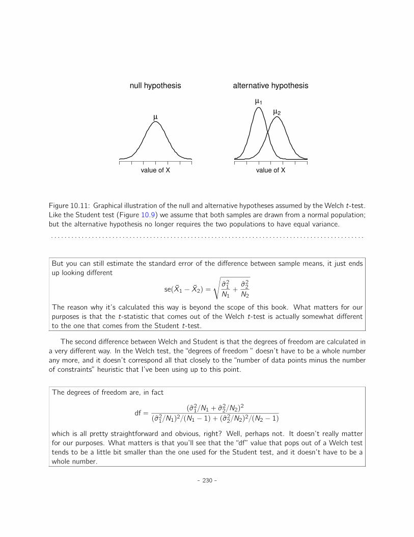
µ

null hypothesis

value of X

µ1

µ2


value of X

Figure 10.11: Graphical illustration of the null and alternative hypotheses assumed by the Welch t-test.Like the Student test (Figure 10.9) we assume that both samples are drawn from a normal population;but the alternative hypothesis no longer requires the two populations to have equal variance.

. . . . . . . . . . . . . . . . . . . . . . . . . . . . . . . . . . . . . . . . . . . . . . . . . . . . . . . . . . . . . . . . . . . . . . . . . . . . . . . . . . . . . . . . . . . .

But you can still estimate the standard error of the difference between sample means, it just endsup looking different

sepX1 ´ X2q “

d

σ21

N1`σ2

2

N2

The reason why it’s calculated this way is beyond the scope of this book. What matters for ourpurposes is that the t-statistic that comes out of the Welch t-test is actually somewhat differentto the one that comes from the Student t-test.

The second difference between Welch and Student is that the degrees of freedom are calculated ina very different way. In the Welch test, the “degrees of freedom ” doesn’t have to be a whole numberany more, and it doesn’t correspond all that closely to the “number of data points minus the numberof constraints” heuristic that I’ve been using up to this point.

The degrees of freedom are, in fact

df “pσ2

1{N1 ` σ22{N2q

2

pσ21{N1q

2{pN1 ´ 1q ` pσ22{N2q

2{pN2 ´ 1q

which is all pretty straightforward and obvious, right? Well, perhaps not. It doesn’t really matterfor our purposes. What matters is that you’ll see that the “df” value that pops out of a Welch testtends to be a little bit smaller than the one used for the Student test, and it doesn’t have to be awhole number.

- 230 -

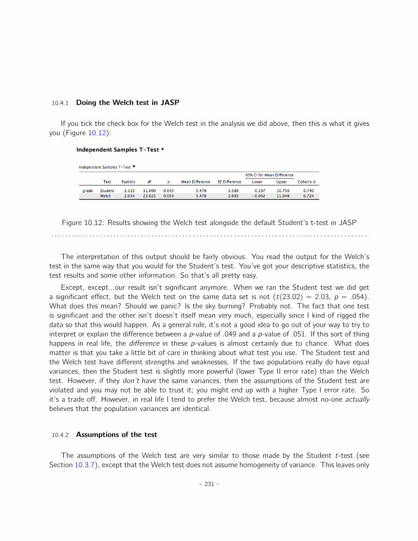
10.4.1 Doing the Welch test in JASP

If you tick the check box for the Welch test in the analysis we did above, then this is what it givesyou (Figure 10.12):

Figure 10.12: Results showing the Welch test alongside the default Student’s t-test in JASP

. . . . . . . . . . . . . . . . . . . . . . . . . . . . . . . . . . . . . . . . . . . . . . . . . . . . . . . . . . . . . . . . . . . . . . . . . . . . . . . . . . . . . . . . . . . .

The interpretation of this output should be fairly obvious. You read the output for the Welch’stest in the same way that you would for the Student’s test. You’ve got your descriptive statistics, thetest results and some other information. So that’s all pretty easy.

Except, except...our result isn’t significant anymore. When we ran the Student test we did geta significant effect, but the Welch test on the same data set is not (tp23.02q “ 2.03, p “ .054).What does this mean? Should we panic? Is the sky burning? Probably not. The fact that one testis significant and the other isn’t doesn’t itself mean very much, especially since I kind of rigged thedata so that this would happen. As a general rule, it’s not a good idea to go out of your way to try tointerpret or explain the difference between a p-value of .049 and a p-value of .051. If this sort of thinghappens in real life, the difference in these p-values is almost certainly due to chance. What doesmatter is that you take a little bit of care in thinking about what test you use. The Student test andthe Welch test have different strengths and weaknesses. If the two populations really do have equalvariances, then the Student test is slightly more powerful (lower Type II error rate) than the Welchtest. However, if they don’t have the same variances, then the assumptions of the Student test areviolated and you may not be able to trust it; you might end up with a higher Type I error rate. Soit’s a trade off. However, in real life I tend to prefer the Welch test, because almost no-one actuallybelieves that the population variances are identical.

10.4.2 Assumptions of the test

The assumptions of the Welch test are very similar to those made by the Student t-test (seeSection 10.3.7), except that the Welch test does not assume homogeneity of variance. This leaves only

- 231 -

the assumption of normality and the assumption of independence. The specifics of these assumptionsare the same for the Welch test as for the Student test.

10.5

The paired-samples t-test

Regardless of whether we’re talking about the Student test or the Welch test, an independent samplest-test is intended to be used in a situation where you have two samples that are, well, independentof one another. This situation arises naturally when participants are assigned randomly to one of twoexperimental conditions, but it provides a very poor approximation to other sorts of research designs.In particular, a repeated measures design, in which each participant is measured (with respect to thesame outcome variable) in both experimental conditions, is not suited for analysis using independentsamples t-tests. For example, we might be interested in whether listening to music reduces people’sworking memory capacity. To that end, we could measure each person’s working memory capacityin two conditions: with music, and without music. In an experimental design such as this one, eachparticipant appears in both groups. This requires us to approach the problem in a different way, byusing the paired samples t-test.

10.5.1 The data

The data set that we’ll use this time comes from Dr Chico’s class.9 In her class students take twomajor tests, one early in the semester and one later in the semester. To hear her tell it, she runs avery hard class, one that most students find very challenging. But she argues that by setting hardassessments students are encouraged to work harder. Her theory is that the first test is a bit of a“wake up call” for students. When they realise how hard her class really is, they’ll work harder for thesecond test and get a better mark. Is she right? To test this, let’s import the chico.csv file intoJASP. The chico data set contains three variables: an id variable that identifies each student in theclass, the grade_test1 variable that records the student grade for the first test, and the grade_test2variable that has the grades for the second test.

If we look at the JASP spreadsheet it does seem like the class is a hard one (most grades arebetween 50% and 60%), but it does look like there’s an improvement from the first test to the secondone.

If we take a quick look at the descriptive statistics, in Figure 10.13, we see that this impressionseems to be supported. Across all 20 students the mean grade for the first test is 57%, but this rises to58% for the second test. Although, given that the standard deviations are 6.6% and 6.4% respectively,it’s starting to feel like maybe the improvement is just illusory; maybe just random variation. This

9At this point we have Drs Harpo, Chico and Zeppo. No prizes for guessing who Dr Groucho is.

- 232 -

Figure 10.13: Descriptives for the two grade_test variables in the chico data set

. . . . . . . . . . . . . . . . . . . . . . . . . . . . . . . . . . . . . . . . . . . . . . . . . . . . . . . . . . . . . . . . . . . . . . . . . . . . . . . . . . . . . . . . . . . .

impression is reinforced when you see the means and confidence intervals plotted in Figure 10.14a. Ifwe were to rely on this plot alone, looking at how wide those confidence intervals are, we’d be temptedto think that the apparent improvement in student performance is pure chance.

Nevertheless, this impression is wrong. To see why, take a look at the scatterplot of the gradesfor test 1 against the grades for test 2, shown in Figure 10.14b. In this plot each dot corresponds tothe two grades for a given student. If their grade for test 1 (x co-ordinate) equals their grade for test2 (y co-ordinate), then the dot falls on the line. Points falling above the line are the students thatperformed better on the second test. Critically, almost all of the data points fall above the diagonalline: almost all of the students do seem to have improved their grade, if only by a small amount.This suggests that we should be looking at the improvement made by each student from one test tothe next and treating that as our raw data. To do this, we’ll need to create a new variable for theimprovement that each student makes, and add it to the chico data set. The easiest way to do thisis to compute a new variable. In JASP, click on the “+” at the right-most side of the data columns,name the variable improvement, and select the “R” button. After you click the ‘Create column’ button,you can enter the R code grade_test2 - grade_test1 (see Figure 10.15).

Once we have computed this new improvement variable we can draw a histogram showing the

- 233 -

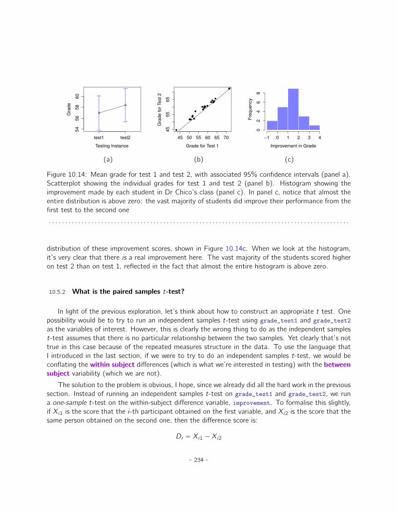
54

56

58

60

Testing Instance

Gra

de

test1 test2 45 50 55 60 65 70

45

55

65

Grade for Test 1

Gra

de

fo

r Te

st

2

Improvement in Grade

Fre

qu

en

cy

−1 0 1 2 3 4

02

46

8

(a) (b) (c)

Figure 10.14: Mean grade for test 1 and test 2, with associated 95% confidence intervals (panel a).Scatterplot showing the individual grades for test 1 and test 2 (panel b). Histogram showing theimprovement made by each student in Dr Chico’s class (panel c). In panel c, notice that almost theentire distribution is above zero: the vast majority of students did improve their performance from thefirst test to the second one

. . . . . . . . . . . . . . . . . . . . . . . . . . . . . . . . . . . . . . . . . . . . . . . . . . . . . . . . . . . . . . . . . . . . . . . . . . . . . . . . . . . . . . . . . . . .

distribution of these improvement scores, shown in Figure 10.14c. When we look at the histogram,it’s very clear that there is a real improvement here. The vast majority of the students scored higheron test 2 than on test 1, reflected in the fact that almost the entire histogram is above zero.

10.5.2 What is the paired samples t-test?

In light of the previous exploration, let’s think about how to construct an appropriate t test. Onepossibility would be to try to run an independent samples t-test using grade_test1 and grade_test2as the variables of interest. However, this is clearly the wrong thing to do as the independent samplest-test assumes that there is no particular relationship between the two samples. Yet clearly that’s nottrue in this case because of the repeated measures structure in the data. To use the language thatI introduced in the last section, if we were to try to do an independent samples t-test, we would beconflating the within subject differences (which is what we’re interested in testing) with the betweensubject variability (which we are not).

The solution to the problem is obvious, I hope, since we already did all the hard work in the previoussection. Instead of running an independent samples t-test on grade_test1 and grade_test2, we runa one-sample t-test on the within-subject difference variable, improvement. To formalise this slightly,if Xi1 is the score that the i-th participant obtained on the first variable, and Xi2 is the score that thesame person obtained on the second one, then the difference score is:

Di “ Xi1 ´Xi2

- 234 -

Figure 10.15: Using R code to compute an improvement score in JASP.

. . . . . . . . . . . . . . . . . . . . . . . . . . . . . . . . . . . . . . . . . . . . . . . . . . . . . . . . . . . . . . . . . . . . . . . . . . . . . . . . . . . . . . . . . . . .

Notice that the difference scores is variable 1 minus variable 2 and not the other way around, so ifwe want improvement to correspond to a positive valued difference, we actually want “test 2” to beour “variable 1”. Equally, we would say that µD “ µ1 ´ µ2 is the population mean for this differencevariable. So, to convert this to a hypothesis test, our null hypothesis is that this mean difference iszero and the alternative hypothesis is that it is not

H0 : µD “ 0

H1 : µD ‰ 0

This is assuming we’re talking about a two-sided test here. This is more or less identical to the waywe described the hypotheses for the one-sample t-test. The only difference is that the specific valuethat the null hypothesis predicts is 0. And so our t-statistic is defined in more or less the same waytoo. If we let D denote the mean of the difference scores, then

t “D

sepDq

which is

t “D

σD{?N

- 235 -

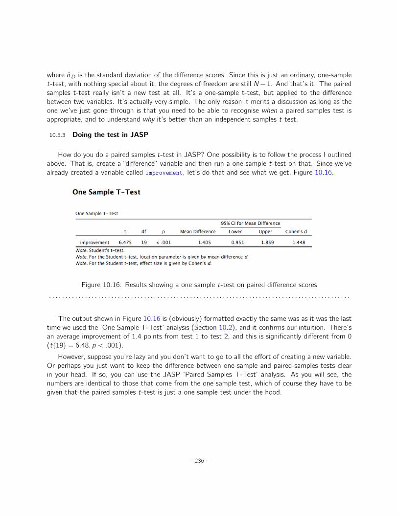
where σD is the standard deviation of the difference scores. Since this is just an ordinary, one-samplet-test, with nothing special about it, the degrees of freedom are still N´ 1. And that’s it. The pairedsamples t-test really isn’t a new test at all. It’s a one-sample t-test, but applied to the differencebetween two variables. It’s actually very simple. The only reason it merits a discussion as long as theone we’ve just gone through is that you need to be able to recognise when a paired samples test isappropriate, and to understand why it’s better than an independent samples t test.


How do you do a paired samples t-test in JASP? One possibility is to follow the process I outlinedabove. That is, create a “difference” variable and then run a one sample t-test on that. Since we’vealready created a variable called improvement, let’s do that and see what we get, Figure 10.16.

Figure 10.16: Results showing a one sample t-test on paired difference scores

. . . . . . . . . . . . . . . . . . . . . . . . . . . . . . . . . . . . . . . . . . . . . . . . . . . . . . . . . . . . . . . . . . . . . . . . . . . . . . . . . . . . . . . . . . . .

The output shown in Figure 10.16 is (obviously) formatted exactly the same was as it was the lasttime we used the ‘One Sample T-Test’ analysis (Section 10.2), and it confirms our intuition. There’san average improvement of 1.4 points from test 1 to test 2, and this is significantly different from 0(tp19q “ 6.48, p ă .001).

However, suppose you’re lazy and you don’t want to go to all the effort of creating a new variable.Or perhaps you just want to keep the difference between one-sample and paired-samples tests clearin your head. If so, you can use the JASP ‘Paired Samples T-Test’ analysis. As you will see, thenumbers are identical to those that come from the one sample test, which of course they have to begiven that the paired samples t-test is just a one sample test under the hood.

- 236 -

10.6

One sided tests

When introducing the theory of null hypothesis tests, I mentioned that there are some situations whenit’s appropriate to specify a one-sided test (see Section 8.4.3). So far all of the t-tests have beentwo-sided tests. For instance, when we specified a one sample t-test for the grades in Dr Zeppo’sclass the null hypothesis was that the true mean was 67.5%. The alternative hypothesis was that thetrue mean was greater than or less than 67.5%. Suppose we were only interested in finding out if thetrue mean is greater than 67.5%, and have no interest whatsoever in testing to find out if the truemean is lower than 67.5%. If so, our null hypothesis would be that the true mean is 67.5% or less,and the alternative hypothesis would be that the true mean is greater than 67.5%. In JASP, for the‘One Sample T-Test’ analysis, you can specify this by clicking on the ‘ą Test Value’ option, under‘Alt. Hypothesis’. When you have done this, you will get the results as shown in 10.17.

Figure 10.17: JASP results showing a ‘One Sample T-Test’ where the actual hypothesis is one sided,i.e. that the true mean is greater than 67.5%

. . . . . . . . . . . . . . . . . . . . . . . . . . . . . . . . . . . . . . . . . . . . . . . . . . . . . . . . . . . . . . . . . . . . . . . . . . . . . . . . . . . . . . . . . . . .

Notice that there are a few changes from the output that we saw last time. Most important is thefact that the actual hypothesis has changed, to reflect the different test. The second thing to noteis that although the t-statistic and degrees of freedom have not changed, the p-value has. This isbecause the one-sided test has a different rejection region from the two-sided test. If you’ve forgottenwhy this is and what it means, you may find it helpful to read back over Chapter 8, and Section 8.4.3in particular. The third thing to note is that the confidence interval is different too: it now reports a“one-sided” confidence interval rather than a two-sided one. In a two-sided confidence interval we’retrying to find numbers a and b such that we’re confident that, if we were to repeat the study manytimes, then 95% of the time the mean would lie between a and b. In a one-sided confidence interval,

- 237 -

we’re trying to find a single number a such that we’re confident that 95% of the time the true meanwould be greater than a (or less than a if you selected ‘ă Test Value’ in the ‘Alt. Hypothesis’ section).

So that’s how to do a one-sided one sample t-test. However, all versions of the t-test can beone-sided. For an independent samples t test, you could have a one-sided test if you’re only interestedin testing to see if group A has higher scores than group B, but have no interest in finding out ifgroup B has higher scores than group A. Let’s suppose that, for Dr Harpo’s class, you wanted to seeif Anastasia’s students had higher grades than Bernadette’s. For this analysis, in the ‘Alt. Hypothesis’options, specify that ‘Group 1 ą Group2’. You should get the results shown in Figure 10.18.

Figure 10.18: JASP results showing an ‘Independent Samples T-Test’ where the actual hypothesis isone sided, i.e. that Anastasia’s students had higher grades than Bernadette’s

. . . . . . . . . . . . . . . . . . . . . . . . . . . . . . . . . . . . . . . . . . . . . . . . . . . . . . . . . . . . . . . . . . . . . . . . . . . . . . . . . . . . . . . . . . . .

Again, the output changes in a predictable way. The definition of the alternative hypothesis haschanged, the p-value has changed, and it now reports a one-sided confidence interval rather than atwo-sided one.

What about the paired samples t-test? Suppose we wanted to test the hypothesis that gradesgo up from test 1 to test 2 in Dr Chico’s class, and are not prepared to consider the idea that thegrades go down. In JASP you would do this by specifying, under the ‘Alt. Hypotheses’ option, thatgrade_test2 (‘Measure 1’ in JASP, because we copied this first into the paired variables box) ągrade_test1 (‘Measure 2’ in JASP). You should get the results shown in Figure 10.19.

Yet again, the output changes in a predictable way. The hypothesis has changed, the p-value haschanged, and the confidence interval is now one-sided.

10.7

Effect size

The most commonly used measure of effect size for a t-test is Cohen’s d (Cohen 1988). It’s a verysimple measure in principle, with quite a few wrinkles when you start digging into the details. Cohenhimself defined it primarily in the context of an independent samples t-test, specifically the Student

- 238 -

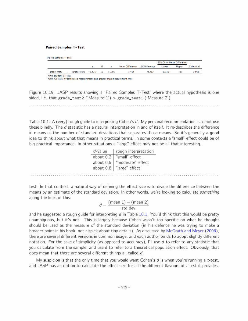
Figure 10.19: JASP results showing a ‘Paired Samples T-Test’ where the actual hypothesis is onesided, i.e. that grade_test2 (‘Measure 1’) ą grade_test1 (‘Measure 2’)

. . . . . . . . . . . . . . . . . . . . . . . . . . . . . . . . . . . . . . . . . . . . . . . . . . . . . . . . . . . . . . . . . . . . . . . . . . . . . . . . . . . . . . . . . . . .

Table 10.1: A (very) rough guide to interpreting Cohen’s d . My personal recommendation is to not usethese blindly. The d statistic has a natural interpretation in and of itself. It re-describes the differencein means as the number of standard deviations that separates those means. So it’s generally a goodidea to think about what that means in practical terms. In some contexts a “small” effect could be ofbig practical importance. In other situations a “large” effect may not be all that interesting.

d-value rough interpretationabout 0.2 “small” effectabout 0.5 “moderate” effectabout 0.8 “large” effect

. . . . . . . . . . . . . . . . . . . . . . . . . . . . . . . . . . . . . . . . . . . . . . . . . . . . . . . . . . . . . . . . . . . . . . . . . . . . . . . . . . . . . . . . . . . .

test. In that context, a natural way of defining the effect size is to divide the difference between themeans by an estimate of the standard deviation. In other words, we’re looking to calculate somethingalong the lines of this:

d “(mean 1)´ (mean 2)

std devand he suggested a rough guide for interpreting d in Table 10.1. You’d think that this would be prettyunambiguous, but it’s not. This is largely because Cohen wasn’t too specific on what he thoughtshould be used as the measure of the standard deviation (in his defence he was trying to make abroader point in his book, not nitpick about tiny details). As discussed by McGrath and Meyer (2006),there are several different versions in common usage, and each author tends to adopt slightly differentnotation. For the sake of simplicity (as opposed to accuracy), I’ll use d to refer to any statistic thatyou calculate from the sample, and use δ to refer to a theoretical population effect. Obviously, thatdoes mean that there are several different things all called d .

My suspicion is that the only time that you would want Cohen’s d is when you’re running a t-test,and JASP has an option to calculate the effect size for all the different flavours of t-test it provides.

- 239 -

10.7.1 Cohen’s d from one sample

The simplest situation to consider is the one corresponding to a one-sample t-test. In this case,this is the one sample mean X and one (hypothesised) population mean µo to compare it to. Notonly that, there’s really only one sensible way to estimate the population standard deviation. We justuse our usual estimate σ. Therefore, we end up with the following as the only way to calculate d

d “X ´ µ0

σ

When we look back at the results in Figure 10.6, the effect size value is Cohen’s d = 0.504. Overall,then, the psychology students in Dr Zeppo’s class are achieving grades (mean = 72.3%) that areabout 0.5 standard deviations higher than the level that you’d expect (67.5%) if they were performingat the same level as other students. Judged against Cohen’s rough guide, this is a moderate effectsize.

10.7.2 Cohen’s d from a Student’s t test

The majority of discussions of Cohen’s d focus on a situation that is analogous to Student’sindependent samples t test, and it’s in this context that the story becomes messier, since there areseveral different versions of d that you might want to use in this situation. To understand why thereare multiple versions of d , it helps to take the time to write down a formula that corresponds to thetrue population effect size δ. It’s pretty straightforward,

δ “µ1 ´ µ2

σ

where, as usual, µ1 and µ2 are the population means corresponding to group 1 and group 2 respectively,and σ is the standard deviation (the same for both populations). The obvious way to estimate δ is todo exactly the same thing that we did in the t-test itself, i.e., use the sample means as the top lineand a pooled standard deviation estimate for the bottom line

d “X1 ´ X2

σp

where σp is the exact same pooled standard deviation measure that appears in the t-test. This is themost commonly used version of Cohen’s d when applied to the outcome of a Student t-test, and isthe one provided in JASP. It is sometimes referred to as Hedges’ g statistic (Hedges 1981).

However, there are other possibilities which I’ll briefly describe. Firstly, you may have reason to wantto use only one of the two groups as the basis for calculating the standard deviation. This approach(often called Glass’ ∆, pronounced delta) only makes most sense when you have good reason to treatone of the two groups as a purer reflection of “natural variation” than the other. This can happen if,for instance, one of the two groups is a control group. Secondly, recall that in the usual calculationof the pooled standard deviation we divide by N ´ 2 to correct for the bias in the sample variance. In

- 240 -

one version of Cohen’s d this correction is omitted, and instead we divide by N. This version makessense primarily when you’re trying to calculate the effect size in the sample rather than estimating aneffect size in the population. Finally, there is a version based on Hedges and Olkin (1985), who pointout there is a small bias in the usual (pooled) estimation for Cohen’s d . Thus they introduce a smallcorrection by multiplying the usual value of d by pN ´ 3q{pN ´ 2.25q.

In any case, ignoring all those variations that you could make use of if you wanted, let’s have a lookat the default version in JASP. In Figure 10.10 Cohen’s d = 0.740, indicating that the grade scores forstudents in Anastasia’s class are, on average, 0.74 standard deviations higher than the grade scoresfor students in Bernadette’s class. For a Welch test, the estimated effect size is the same (Figure10.12).

10.7.3 Cohen’s d from a paired-samples test

Finally, what should we do for a paired samples t-test? In this case, the answer depends on whatit is you’re trying to do. JASP assumes that you want to measure your effect sizes relative to thedistribution of difference scores, and the measure of d that you calculate is:

d “D

σD

where σD is the estimate of the standard deviation of the differences. In Figure 10.16 Cohen’s d =1.45, indicating that the time 2 grade scores are, on average, 1.45 standard deviations higher thanthe time 1 grade scores.

This is the version of Cohen’s d that gets reported by the JASP ‘Paired Samples T-Test’ analysis.The only wrinkle is figuring out whether this is the measure you want or not. To the extent that youcare about the practical consequences of your research, you often want to measure the effect sizerelative to the original variables, not the difference scores (e.g., the 1 point improvement in Dr Chico’sclass over time is pretty small when measured against the amount of between-student variation ingrades), in which case you use the same versions of Cohen’s d that you would use for a Student orWelch test. It’s not so straightforward to do this in JASP; essentially you have to change the structureof the data in the spreadsheet view so I won’t go into that here.

10.8

Checking the normality of a sample

All of the tests that we have discussed so far in this chapter have assumed that the data are nor-mally distributed. This assumption is often quite reasonable, because the central limit theorem (Sec-tion 7.3.3) does tend to ensure that many real world quantities are normally distributed. Any timethat you suspect that your variable is actually an average of lots of different things, there’s a prettygood chance that it will be normally distributed, or at least close enough to normal that you can getaway with using t-tests. However, life doesn’t come with guarantees, and besides there are lots ofways in which you can end up with variables that are highly non-normal. For example, any time you

- 241 -

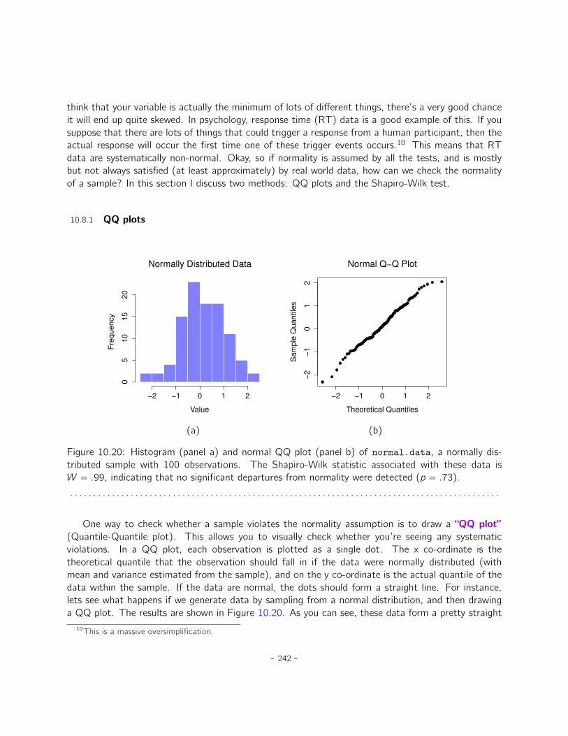
think that your variable is actually the minimum of lots of different things, there’s a very good chanceit will end up quite skewed. In psychology, response time (RT) data is a good example of this. If yousuppose that there are lots of things that could trigger a response from a human participant, then theactual response will occur the first time one of these trigger events occurs.10 This means that RTdata are systematically non-normal. Okay, so if normality is assumed by all the tests, and is mostlybut not always satisfied (at least approximately) by real world data, how can we check the normalityof a sample? In this section I discuss two methods: QQ plots and the Shapiro-Wilk test.

10.8.1 QQ plots

Normally Distributed Data

Value

Fre

qu

en

cy

−2 −1 0 1 2

05

10

15

20

−2 −1 0 1 2

−2

−1

01

2

Normal Q−Q Plot

Theoretical Quantiles

Sa

mp

le Q

ua

ntile

s

(a) (b)

Figure 10.20: Histogram (panel a) and normal QQ plot (panel b) of normal.data, a normally dis-tributed sample with 100 observations. The Shapiro-Wilk statistic associated with these data isW “ .99, indicating that no significant departures from normality were detected (p “ .73).

. . . . . . . . . . . . . . . . . . . . . . . . . . . . . . . . . . . . . . . . . . . . . . . . . . . . . . . . . . . . . . . . . . . . . . . . . . . . . . . . . . . . . . . . . . . .

One way to check whether a sample violates the normality assumption is to draw a “QQ plot”(Quantile-Quantile plot). This allows you to visually check whether you’re seeing any systematicviolations. In a QQ plot, each observation is plotted as a single dot. The x co-ordinate is thetheoretical quantile that the observation should fall in if the data were normally distributed (withmean and variance estimated from the sample), and on the y co-ordinate is the actual quantile of thedata within the sample. If the data are normal, the dots should form a straight line. For instance,lets see what happens if we generate data by sampling from a normal distribution, and then drawinga QQ plot. The results are shown in Figure 10.20. As you can see, these data form a pretty straight

10This is a massive oversimplification.

- 242 -

Skewed Data

Value

Fre

qu

en

cy

0.0 0.5 1.0 1.5 2.0 2.5

01

02

03

04

05

06

0

−2 −1 0 1 2

0.0

0.5

1.0

1.5

2.0

Normal Q−Q Plot


Sa

mp

le Q

ua

ntile

s(a) (b)

Heavy−Tailed Data

Value

Fre

qu

en

cy

−6 −4 −2 0 2 4 6 8

01

02

03

04

0

−2 −1 0 1 2

−6

−4

−2

02

46

Normal Q−Q Plot


Sa

mp

le Q

ua

ntile

s

(c) (d)

Figure 10.21: In the top row, a histogram (panel a) and normal QQ plot (panel b) of the 100observations in a skewed.data set. The skewness of the data here is 1.94, and is reflected in aQQ plot that curves upwards. As a consequence, the Shapiro-Wilk statistic is W “ .80, reflecting asignificant departure from normality (p ă .001). The bottom row shows the same plots for a heavytailed data set, again consisting of 100 observations. In this case the heavy tails in the data producea high kurtosis (2.80), and cause the QQ plot to flatten in the middle, and curve away sharply oneither side. The resulting Shapiro-Wilk statistic is W “ .93, again reflecting significant non-normality(p ă .001).

. . . . . . . . . . . . . . . . . . . . . . . . . . . . . . . . . . . . . . . . . . . . . . . . . . . . . . . . . . . . . . . . . . . . . . . . . . . . . . . . . . . . . . . . . . . .

- 243 -

line; which is no surprise given that we sampled them from a normal distribution! In contrast, have alook at the two data sets shown in Figure 10.21. The top panels show the histogram and a QQ plotfor a data set that is highly skewed: the QQ plot curves upwards. The lower panels show the sameplots for a heavy tailed (i.e., high kurtosis) data set: in this case the QQ plot flattens in the middleand curves sharply at either end.

10.8.2 Shapiro-Wilk tests

QQ plots provide a nice way to informally check the normality of your data, but sometimes you’llwant to do something a bit more formal and the Shapiro-Wilk test (Shapiro and Wilk 1965) isprobably what you’re looking for.11 As you’d expect, the null hypothesis being tested is that a set ofN observations is normally distributed.

The test statistic that it calculates is conventionally denoted as W , and it’s calculated as follows.First, we sort the observations in order of increasing size, and let X1 be the smallest value in thesample, X2 be the second smallest and so on. Then the value of W is given by

W “

´

řNi“1 aiXi

¯2

řNi“1pXi ´ Xq

2

where X is the mean of the observations, and the ai values are ... mumble, mumble ... somethingcomplicated that is a bit beyond the scope of an introductory text.

Because it’s a little hard to explain the maths behind the W statistic, a better idea is to give abroad brush description of how it behaves. Unlike most of the test statistics that we’ll encounter inthis book, it’s actually small values of W that indicate departure from normality. The W statistic hasa maximum value of 1, which occurs when the data look “perfectly normal”. The smaller the value ofW the less normal the data are. However, the sampling distribution for W , which is not one of thestandard ones that I discussed in Chapter 6 and is in fact a complete pain in the arse to work with,does depend on the sample size N. To give you a feel for what these sampling distributions look like,I’ve plotted three of them in Figure 10.22. Notice that, as the sample size starts to get large, thesampling distribution becomes very tightly clumped up near W “ 1, and as a consequence, for largersamples W doesn’t have to be very much smaller than 1 in order for the test to be significant.

To get the Shapiro-Wilk statistic in JASP t-tests, check the option for ‘Normality’ listed under‘Assumption checks’. In the randomly sampled data (N = 100) we used for the QQ plot, the value forthe Shapiro-Wilk normality test statistic was W = 0.99 with a p-value of 0.69. So, not surprisingly, we

11Either that, or the Kolmogorov-Smirnov test, which is probably more traditional than the Shapiro-Wilk. Althoughmost things I’ve read seem to suggest Shapiro-Wilk is the better test of normality, the Kolomogorov- Smirnov is a generalpurpose test of distributional equivalence that can be adapted to handle other kinds of distribution tests. In JASP theShapiro-Wilk test is preferred.

- 244 -

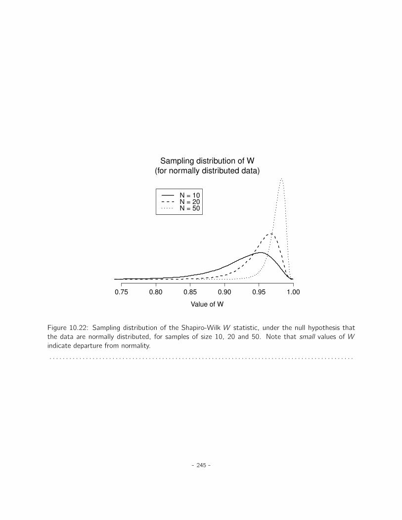
0.75 0.80 0.85 0.90 0.95 1.00

Sampling distribution of W

(for normally distributed data)

Value of W

N = 10N = 20N = 50

Figure 10.22: Sampling distribution of the Shapiro-Wilk W statistic, under the null hypothesis thatthe data are normally distributed, for samples of size 10, 20 and 50. Note that small values of Windicate departure from normality.

. . . . . . . . . . . . . . . . . . . . . . . . . . . . . . . . . . . . . . . . . . . . . . . . . . . . . . . . . . . . . . . . . . . . . . . . . . . . . . . . . . . . . . . . . . . .

- 245 -

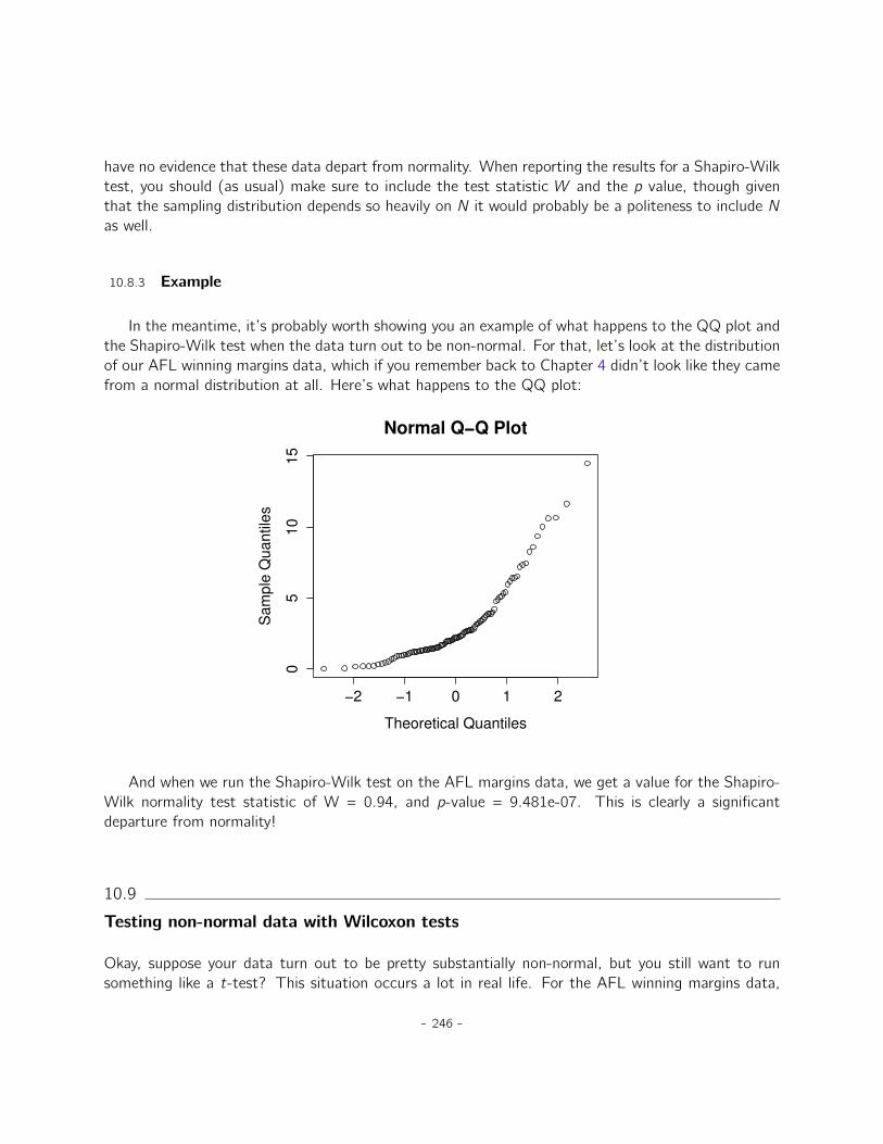
have no evidence that these data depart from normality. When reporting the results for a Shapiro-Wilktest, you should (as usual) make sure to include the test statistic W and the p value, though giventhat the sampling distribution depends so heavily on N it would probably be a politeness to include Nas well.

10.8.3 Example

In the meantime, it’s probably worth showing you an example of what happens to the QQ plot andthe Shapiro-Wilk test when the data turn out to be non-normal. For that, let’s look at the distributionof our AFL winning margins data, which if you remember back to Chapter 4 didn’t look like they camefrom a normal distribution at all. Here’s what happens to the QQ plot:

−2 −1 0 1 2

05

10

15

Normal Q−Q Plot


Sam

ple

Quantile

s

And when we run the Shapiro-Wilk test on the AFL margins data, we get a value for the Shapiro-Wilk normality test statistic of W = 0.94, and p-value = 9.481e-07. This is clearly a significantdeparture from normality!

10.9

Testing non-normal data with Wilcoxon tests

Okay, suppose your data turn out to be pretty substantially non-normal, but you still want to runsomething like a t-test? This situation occurs a lot in real life. For the AFL winning margins data,

- 246 -

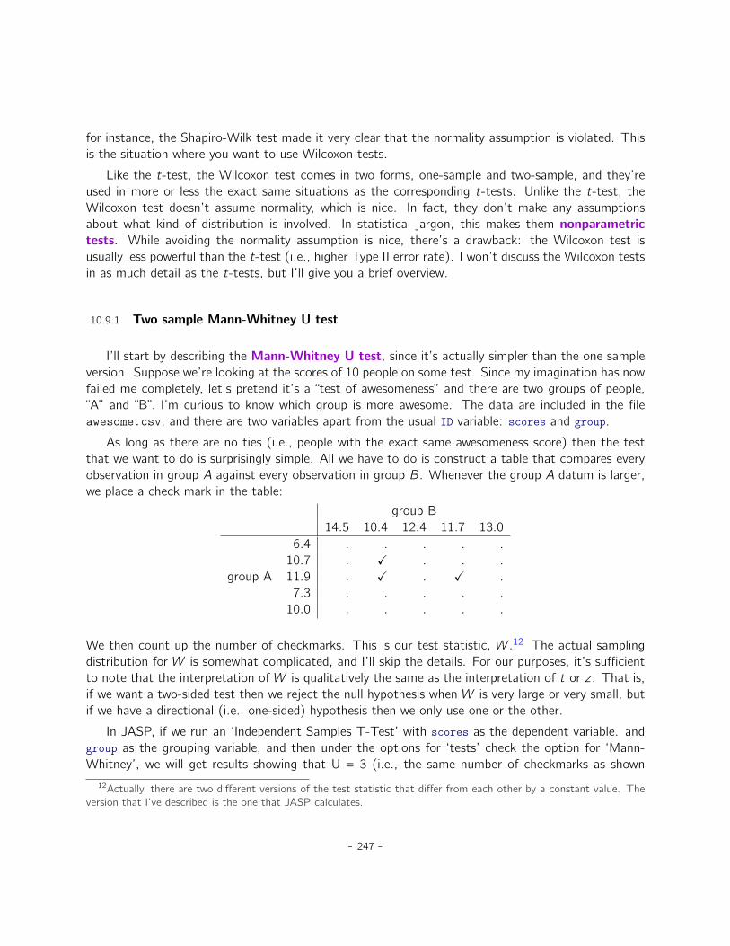
for instance, the Shapiro-Wilk test made it very clear that the normality assumption is violated. Thisis the situation where you want to use Wilcoxon tests.

Like the t-test, the Wilcoxon test comes in two forms, one-sample and two-sample, and they’reused in more or less the exact same situations as the corresponding t-tests. Unlike the t-test, theWilcoxon test doesn’t assume normality, which is nice. In fact, they don’t make any assumptionsabout what kind of distribution is involved. In statistical jargon, this makes them nonparametrictests. While avoiding the normality assumption is nice, there’s a drawback: the Wilcoxon test isusually less powerful than the t-test (i.e., higher Type II error rate). I won’t discuss the Wilcoxon testsin as much detail as the t-tests, but I’ll give you a brief overview.

10.9.1 Two sample Mann-Whitney U test

I’ll start by describing the Mann-Whitney U test, since it’s actually simpler than the one sampleversion. Suppose we’re looking at the scores of 10 people on some test. Since my imagination has nowfailed me completely, let’s pretend it’s a “test of awesomeness” and there are two groups of people,“A” and “B”. I’m curious to know which group is more awesome. The data are included in the fileawesome.csv, and there are two variables apart from the usual ID variable: scores and group.

As long as there are no ties (i.e., people with the exact same awesomeness score) then the testthat we want to do is surprisingly simple. All we have to do is construct a table that compares everyobservation in group A against every observation in group B. Whenever the group A datum is larger,we place a check mark in the table:

group B14.5 10.4 12.4 11.7 13.0

6.4 . . . . .10.7 . X . . .

group A 11.9 . X . X .7.3 . . . . .10.0 . . . . .

We then count up the number of checkmarks. This is our test statistic, W .12 The actual samplingdistribution for W is somewhat complicated, and I’ll skip the details. For our purposes, it’s sufficientto note that the interpretation of W is qualitatively the same as the interpretation of t or z . That is,if we want a two-sided test then we reject the null hypothesis when W is very large or very small, butif we have a directional (i.e., one-sided) hypothesis then we only use one or the other.

In JASP, if we run an ‘Independent Samples T-Test’ with scores as the dependent variable. andgroup as the grouping variable, and then under the options for ‘tests’ check the option for ‘Mann-Whitney’, we will get results showing that U = 3 (i.e., the same number of checkmarks as shown

12Actually, there are two different versions of the test statistic that differ from each other by a constant value. Theversion that I’ve described is the one that JASP calculates.

- 247 -

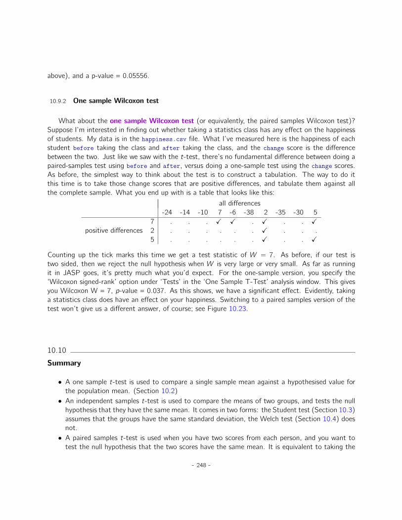
above), and a p-value = 0.05556.

10.9.2 One sample Wilcoxon test

What about the one sample Wilcoxon test (or equivalently, the paired samples Wilcoxon test)?Suppose I’m interested in finding out whether taking a statistics class has any effect on the happinessof students. My data is in the happiness.csv file. What I’ve measured here is the happiness of eachstudent before taking the class and after taking the class, and the change score is the differencebetween the two. Just like we saw with the t-test, there’s no fundamental difference between doing apaired-samples test using before and after, versus doing a one-sample test using the change scores.As before, the simplest way to think about the test is to construct a tabulation. The way to do itthis time is to take those change scores that are positive differences, and tabulate them against allthe complete sample. What you end up with is a table that looks like this:

all differences-24 -14 -10 7 -6 -38 2 -35 -30 5

7 . . . X X . X . . Xpositive differences 2 . . . . . . X . . .

5 . . . . . . X . . X

Counting up the tick marks this time we get a test statistic of W “ 7. As before, if our test istwo sided, then we reject the null hypothesis when W is very large or very small. As far as runningit in JASP goes, it’s pretty much what you’d expect. For the one-sample version, you specify the‘Wilcoxon signed-rank’ option under ‘Tests’ in the ‘One Sample T-Test’ analysis window. This givesyou Wilcoxon W = 7, p-value = 0.037. As this shows, we have a significant effect. Evidently, takinga statistics class does have an effect on your happiness. Switching to a paired samples version of thetest won’t give us a different answer, of course; see Figure 10.23.

10.10

Summary

• A one sample t-test is used to compare a single sample mean against a hypothesised value forthe population mean. (Section 10.2)• An independent samples t-test is used to compare the means of two groups, and tests the nullhypothesis that they have the same mean. It comes in two forms: the Student test (Section 10.3)assumes that the groups have the same standard deviation, the Welch test (Section 10.4) doesnot.• A paired samples t-test is used when you have two scores from each person, and you want totest the null hypothesis that the two scores have the same mean. It is equivalent to taking the

- 248 -

Figure 10.23: JASP screen showing results for one sample and paired sample Wilcoxon non-parametrictests

. . . . . . . . . . . . . . . . . . . . . . . . . . . . . . . . . . . . . . . . . . . . . . . . . . . . . . . . . . . . . . . . . . . . . . . . . . . . . . . . . . . . . . . . . . . .

difference between the two scores for each person, and then running a one sample t-test on thedifference scores. (Section 10.5)

• One sided tests are perfectly legitimate as long as they are pre-planned. (Section 10.6)

• Effect size calculations for the difference between means can be calculated via the Cohen’s dstatistic. (Section 10.7).

• You can check the normality of a sample using QQ plots (not currently available in JASP) andthe Shapiro-Wilk test. (Section 10.8)

• If your data are non-normal, you can use Mann-Whitney or Wilcoxon tests instead of t-tests.(Section 10.9)

- 249 -

- 250 -

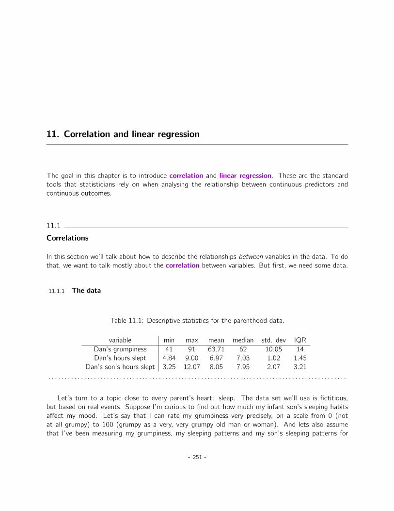
11. Correlation and linear regression

The goal in this chapter is to introduce correlation and linear regression. These are the standardtools that statisticians rely on when analysing the relationship between continuous predictors andcontinuous outcomes.

11.1

Correlations

In this section we’ll talk about how to describe the relationships between variables in the data. To dothat, we want to talk mostly about the correlation between variables. But first, we need some data.

11.1.1 The data

Table 11.1: Descriptive statistics for the parenthood data.

variable min max mean median std. dev IQRDan’s grumpiness 41 91 63.71 62 10.05 14Dan’s hours slept 4.84 9.00 6.97 7.03 1.02 1.45

Dan’s son’s hours slept 3.25 12.07 8.05 7.95 2.07 3.21. . . . . . . . . . . . . . . . . . . . . . . . . . . . . . . . . . . . . . . . . . . . . . . . . . . . . . . . . . . . . . . . . . . . . . . . . . . . . . . . . . . . . . . . . . . .

Let’s turn to a topic close to every parent’s heart: sleep. The data set we’ll use is fictitious,but based on real events. Suppose I’m curious to find out how much my infant son’s sleeping habitsaffect my mood. Let’s say that I can rate my grumpiness very precisely, on a scale from 0 (notat all grumpy) to 100 (grumpy as a very, very grumpy old man or woman). And lets also assumethat I’ve been measuring my grumpiness, my sleeping patterns and my son’s sleeping patterns for

- 251 -

quite some time now. Let’s say, for 100 days. And, being a nerd, I’ve saved the data as a filecalled parenthood.csv. If we load the data into JASP we can see that the file contains four variablesdan.sleep, baby.sleep, dan.grump and day. Note that when you first load this data set JASP maynot have guessed the data type for each variable correctly, in which case you should fix it: dan.sleep,baby.sleep, dan.grump and day can be specified as continuous variables, and ID is a nominal(integer)variable.

Next, I’ll take a look at some basic descriptive statistics and, to give a graphical depiction of whateach of the three interesting variables looks like, Figure 11.1 plots histograms. One thing to note:just because JASP can calculate dozens of different statistics doesn’t mean you should report all ofthem. If I were writing this up for a report, I’d probably pick out those statistics that are of mostinterest to me (and to my readership), and then put them into a nice, simple table like the one inTable 11.1.1 Notice that when I put it into a table, I gave everything “human readable” names. Thisis always good practice. Notice also that I’m not getting enough sleep. This isn’t good practice, butother parents tell me that it’s pretty standard.

My grumpiness

Fre

qu

en

cy

40 50 60 70 80 90

05

10

15

20

My sleep (hours)

Fre

qu

en

cy

5 6 7 8 9

05

10

15

20

The baby’s sleep (hours)

Fre

qu

en

cy

4 6 8 10 12

05

10

15

20

(a) (b) (c)

Figure 11.1: Histograms for the three interesting variables in the parenthood data set.

. . . . . . . . . . . . . . . . . . . . . . . . . . . . . . . . . . . . . . . . . . . . . . . . . . . . . . . . . . . . . . . . . . . . . . . . . . . . . . . . . . . . . . . . . . . .

11.1.2 The strength and direction of a relationship

We can draw scatterplots to give us a general sense of how closely related two variables are. Ideallythough, we might want to say a bit more about it than that. For instance, let’s compare the relationshipbetween dan.sleep and dan.grump (Figure 11.2, left) with that between baby.sleep and dan.grump(Figure 11.2, right). When looking at these two plots side by side, it’s clear that the relationship isqualitatively the same in both cases: more sleep equals less grump! However, it’s also pretty obviousthat the relationship between dan.sleep and dan.grump is stronger than the relationship between

1Actually, even that table is more than I’d bother with. In practice most people pick one measure of central tendency,and one measure of variability only.

- 252 -

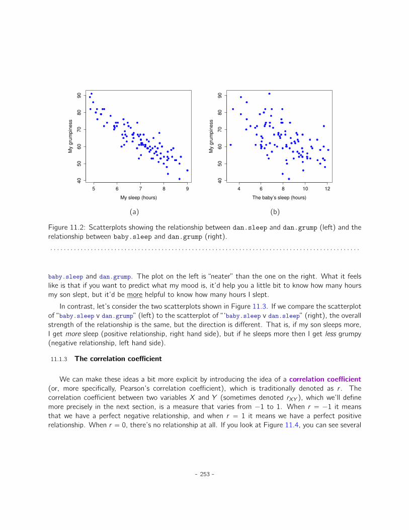
5 6 7 8 9

40

50

60

70

80

90

My sleep (hours)

My g

rum

pin

ess

4 6 8 10 12

40

50

60

70

80

90


My g

rum

pin

ess

(a) (b)

Figure 11.2: Scatterplots showing the relationship between dan.sleep and dan.grump (left) and therelationship between baby.sleep and dan.grump (right).

. . . . . . . . . . . . . . . . . . . . . . . . . . . . . . . . . . . . . . . . . . . . . . . . . . . . . . . . . . . . . . . . . . . . . . . . . . . . . . . . . . . . . . . . . . . .

baby.sleep and dan.grump. The plot on the left is “neater” than the one on the right. What it feelslike is that if you want to predict what my mood is, it’d help you a little bit to know how many hoursmy son slept, but it’d be more helpful to know how many hours I slept.

In contrast, let’s consider the two scatterplots shown in Figure 11.3. If we compare the scatterplotof “baby.sleep v dan.grump” (left) to the scatterplot of “ ‘baby.sleep v dan.sleep” (right), the overallstrength of the relationship is the same, but the direction is different. That is, if my son sleeps more,I get more sleep (positive relationship, right hand side), but if he sleeps more then I get less grumpy(negative relationship, left hand side).

11.1.3 The correlation coefficient

We can make these ideas a bit more explicit by introducing the idea of a correlation coefficient(or, more specifically, Pearson’s correlation coefficient), which is traditionally denoted as r . Thecorrelation coefficient between two variables X and Y (sometimes denoted rXY ), which we’ll definemore precisely in the next section, is a measure that varies from ´1 to 1. When r “ ´1 it meansthat we have a perfect negative relationship, and when r “ 1 it means we have a perfect positiverelationship. When r “ 0, there’s no relationship at all. If you look at Figure 11.4, you can see several

- 253 -

4 6 8 10 12

40

50

60

70

80

90


My g

rum

pin

ess

4 6 8 10 12

56

78

9


My s

lee

p (

ho

urs

)(a) (b)

Figure 11.3: Scatterplots showing the relationship between baby.sleep and dan.grump (left), ascompared to the relationship between baby.sleep and dan.sleep (right).

. . . . . . . . . . . . . . . . . . . . . . . . . . . . . . . . . . . . . . . . . . . . . . . . . . . . . . . . . . . . . . . . . . . . . . . . . . . . . . . . . . . . . . . . . . . .

plots showing what different correlations look like.

The formula for the Pearson’s correlation coefficient can be written in several different ways. I thinkthe simplest way to write down the formula is to break it into two steps. Firstly, let’s introducethe idea of a covariance. The covariance between two variables X and Y is a generalisation of thenotion of the variance amd is a mathematically simple way of describing the relationship betweentwo variables that isn’t terribly informative to humans

CovpX, Y q “1

N ´ 1

Nÿ

i“1

`

Xi ´ X˘ `

Yi ´ Y˘

Because we’re multiplying (i.e., taking the “product” of) a quantity that depends on X by a quantitythat depends on Y and then averaginga, you can think of the formula for the covariance as an

- 254 -

positive correlations negative correlations

0.0 0.0

0.33 ´0.33

0.66 ´0.66

1.0 ´1.0

Figure 11.4: Illustration of the effect of varying the strength and direction of a correlation. In the lefthand column, the correlations are 0, .33, .66 and 1. In the right hand column, the correlations are 0,-.33, -.66 and -1.

. . . . . . . . . . . . . . . . . . . . . . . . . . . . . . . . . . . . . . . . . . . . . . . . . . . . . . . . . . . . . . . . . . . . . . . . . . . . . . . . . . . . . . . . . . . .- 255 -

“average cross product” between X and Y .

The covariance has the nice property that, if X and Y are entirely unrelated, then the covarianceis exactly zero. If the relationship between them is positive (in the sense shown in Figure 11.4) thenthe covariance is also positive, and if the relationship is negative then the covariance is also negative.In other words, the covariance captures the basic qualitative idea of correlation. Unfortunately, theraw magnitude of the covariance isn’t easy to interpret as it depends on the units in which X and Yare expressed and, worse yet, the actual units that the covariance itself is expressed in are really weird.For instance, if X refers to the dan.sleep variable (units: hours) and Y refers to the dan.grumpvariable (units: grumps), then the units for their covariance are “hours ˆ grumps”. And I have nofreaking idea what that would even mean.

The Pearson correlation coefficient r fixes this interpretation problem by standardising the co-variance, in pretty much the exact same way that the z-score standardises a raw score, by dividingby the standard deviation. However, because we have two variables that contribute to the covari-ance, the standardisation only works if we divide by both standard deviations.b In other words, thecorrelation between X and Y can be written as follows:

rXY “CovpX, Y qσX σY

aJust like we saw with the variance and the standard deviation, in practice we divide by N ´ 1 rather than N.bThis is an oversimplification, but it’ll do for our purposes.

By standardising the covariance, not only do we keep all of the nice properties of the covariancediscussed earlier, but the actual values of r are on a meaningful scale: r “ 1 implies a perfect positiverelationship and r “ ´1 implies a perfect negative relationship. I’ll expand a little more on this pointlater, in Section 11.1.5. But before I do, let’s look at how to calculate correlations in JASP.

11.1.4 Calculating correlations in JASP

Calculating correlations in JASP can be done by clicking on the ‘Regression’ - ‘Correlation Matrix’button. Transfer all four continuous variables across into the box on the right to get the output inFigure 11.5. Notice that each correlation (denoted ‘Pearson’s r ’) is paired with a p-value. Clearly,something is being tested here, but ignore it for now. We’ll talk more about that soon!

11.1.5 Interpreting a correlation

Naturally, in real life you don’t see many correlations of 1. So how should you interpret a correlationof, say, r “ .4? The honest answer is that it really depends on what you want to use the data for,and on how strong the correlations in your field tend to be. A friend of mine in engineering onceargued that any correlation less than .95 is completely useless (I think he was exaggerating, even for

- 256 -

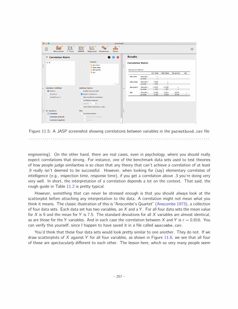
Figure 11.5: A JASP screenshot showing correlations between variables in the parenthood.csv file

. . . . . . . . . . . . . . . . . . . . . . . . . . . . . . . . . . . . . . . . . . . . . . . . . . . . . . . . . . . . . . . . . . . . . . . . . . . . . . . . . . . . . . . . . . . .

engineering). On the other hand, there are real cases, even in psychology, where you should reallyexpect correlations that strong. For instance, one of the benchmark data sets used to test theoriesof how people judge similarities is so clean that any theory that can’t achieve a correlation of at least.9 really isn’t deemed to be successful. However, when looking for (say) elementary correlates ofintelligence (e.g., inspection time, response time), if you get a correlation above .3 you’re doing veryvery well. In short, the interpretation of a correlation depends a lot on the context. That said, therough guide in Table 11.2 is pretty typical.

However, something that can never be stressed enough is that you should always look at thescatterplot before attaching any interpretation to the data. A correlation might not mean what youthink it means. The classic illustration of this is “Anscombe’s Quartet” (Anscombe 1973), a collectionof four data sets. Each data set has two variables, an X and a Y . For all four data sets the mean valuefor X is 9 and the mean for Y is 7.5. The standard deviations for all X variables are almost identical,as are those for the Y variables. And in each case the correlation between X and Y is r “ 0.816. Youcan verify this yourself, since I happen to have saved it in a file called anscombe.csv.

You’d think that these four data sets would look pretty similar to one another. They do not. If wedraw scatterplots of X against Y for all four variables, as shown in Figure 11.6, we see that all fourof these are spectacularly different to each other. The lesson here, which so very many people seem

- 257 -

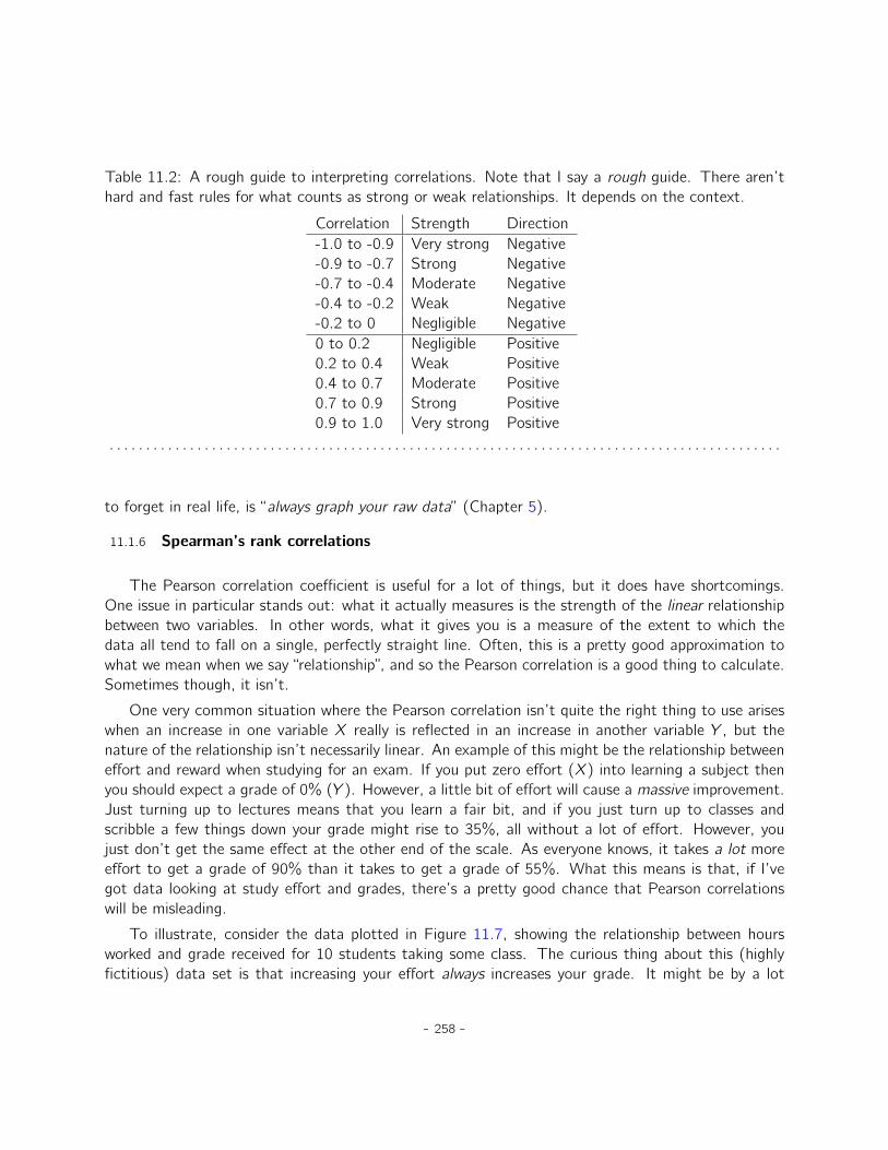
Table 11.2: A rough guide to interpreting correlations. Note that I say a rough guide. There aren’thard and fast rules for what counts as strong or weak relationships. It depends on the context.

Correlation Strength Direction-1.0 to -0.9 Very strong Negative-0.9 to -0.7 Strong Negative-0.7 to -0.4 Moderate Negative-0.4 to -0.2 Weak Negative-0.2 to 0 Negligible Negative0 to 0.2 Negligible Positive0.2 to 0.4 Weak Positive0.4 to 0.7 Moderate Positive0.7 to 0.9 Strong Positive0.9 to 1.0 Very strong Positive

. . . . . . . . . . . . . . . . . . . . . . . . . . . . . . . . . . . . . . . . . . . . . . . . . . . . . . . . . . . . . . . . . . . . . . . . . . . . . . . . . . . . . . . . . . . .

to forget in real life, is “always graph your raw data” (Chapter 5).

11.1.6 Spearman’s rank correlations

The Pearson correlation coefficient is useful for a lot of things, but it does have shortcomings.One issue in particular stands out: what it actually measures is the strength of the linear relationshipbetween two variables. In other words, what it gives you is a measure of the extent to which thedata all tend to fall on a single, perfectly straight line. Often, this is a pretty good approximation towhat we mean when we say “relationship”, and so the Pearson correlation is a good thing to calculate.Sometimes though, it isn’t.

One very common situation where the Pearson correlation isn’t quite the right thing to use ariseswhen an increase in one variable X really is reflected in an increase in another variable Y , but thenature of the relationship isn’t necessarily linear. An example of this might be the relationship betweeneffort and reward when studying for an exam. If you put zero effort (X) into learning a subject thenyou should expect a grade of 0% (Y ). However, a little bit of effort will cause a massive improvement.Just turning up to lectures means that you learn a fair bit, and if you just turn up to classes andscribble a few things down your grade might rise to 35%, all without a lot of effort. However, youjust don’t get the same effect at the other end of the scale. As everyone knows, it takes a lot moreeffort to get a grade of 90% than it takes to get a grade of 55%. What this means is that, if I’vegot data looking at study effort and grades, there’s a pretty good chance that Pearson correlationswill be misleading.

To illustrate, consider the data plotted in Figure 11.7, showing the relationship between hoursworked and grade received for 10 students taking some class. The curious thing about this (highlyfictitious) data set is that increasing your effort always increases your grade. It might be by a lot

- 258 -

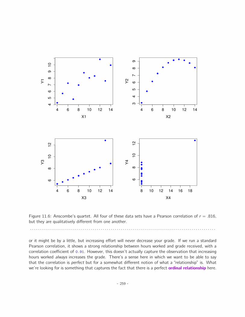
4 6 8 10 12 14

45

67

89

10

X1

Y1

4 6 8 10 12 14

34

56

78

9

X2

Y2

4 6 8 10 12 14

68

10

12

X3

Y3

8 10 12 14 16 18

68

10

12

X4

Y4

Figure 11.6: Anscombe’s quartet. All four of these data sets have a Pearson correlation of r “ .816,but they are qualitatively different from one another.

. . . . . . . . . . . . . . . . . . . . . . . . . . . . . . . . . . . . . . . . . . . . . . . . . . . . . . . . . . . . . . . . . . . . . . . . . . . . . . . . . . . . . . . . . . . .

or it might be by a little, but increasing effort will never decrease your grade. If we run a standardPearson correlation, it shows a strong relationship between hours worked and grade received, with acorrelation coefficient of 0.91. However, this doesn’t actually capture the observation that increasinghours worked always increases the grade. There’s a sense here in which we want to be able to saythat the correlation is perfect but for a somewhat different notion of what a “relationship” is. Whatwe’re looking for is something that captures the fact that there is a perfect ordinal relationship here.

- 259 -

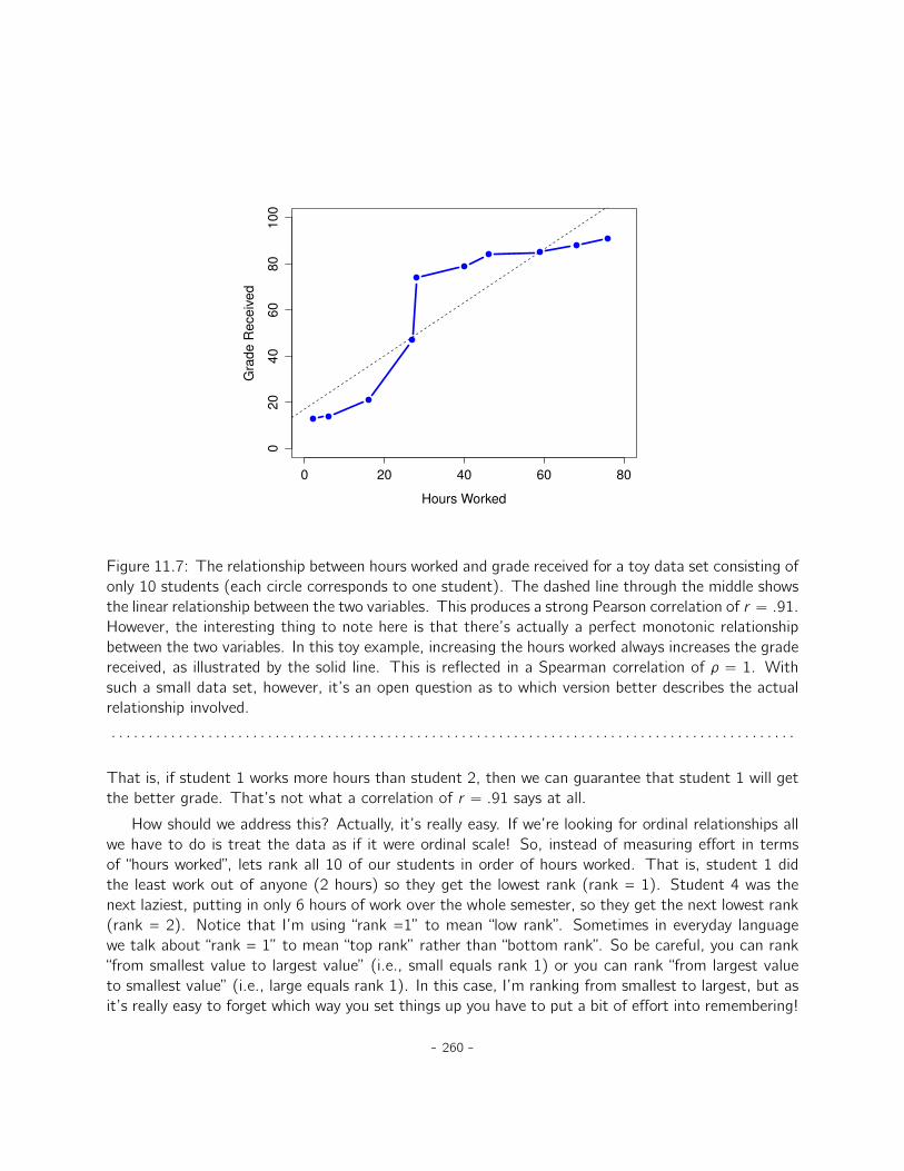
0 20 40 60 80

02

04

06

08

01

00

Hours Worked

Gra

de

Re

ce

ive

d

Figure 11.7: The relationship between hours worked and grade received for a toy data set consisting ofonly 10 students (each circle corresponds to one student). The dashed line through the middle showsthe linear relationship between the two variables. This produces a strong Pearson correlation of r “ .91.However, the interesting thing to note here is that there’s actually a perfect monotonic relationshipbetween the two variables. In this toy example, increasing the hours worked always increases the gradereceived, as illustrated by the solid line. This is reflected in a Spearman correlation of ρ “ 1. Withsuch a small data set, however, it’s an open question as to which version better describes the actualrelationship involved.

. . . . . . . . . . . . . . . . . . . . . . . . . . . . . . . . . . . . . . . . . . . . . . . . . . . . . . . . . . . . . . . . . . . . . . . . . . . . . . . . . . . . . . . . . . . .

That is, if student 1 works more hours than student 2, then we can guarantee that student 1 will getthe better grade. That’s not what a correlation of r “ .91 says at all.

How should we address this? Actually, it’s really easy. If we’re looking for ordinal relationships allwe have to do is treat the data as if it were ordinal scale! So, instead of measuring effort in termsof “hours worked”, lets rank all 10 of our students in order of hours worked. That is, student 1 didthe least work out of anyone (2 hours) so they get the lowest rank (rank = 1). Student 4 was thenext laziest, putting in only 6 hours of work over the whole semester, so they get the next lowest rank(rank = 2). Notice that I’m using “rank =1” to mean “low rank”. Sometimes in everyday languagewe talk about “rank = 1” to mean “top rank” rather than “bottom rank”. So be careful, you can rank“from smallest value to largest value” (i.e., small equals rank 1) or you can rank “from largest valueto smallest value” (i.e., large equals rank 1). In this case, I’m ranking from smallest to largest, but asit’s really easy to forget which way you set things up you have to put a bit of effort into remembering!

- 260 -

Okay, so let’s have a look at our students when we rank them from worst to best in terms of effortand reward:

rank (hours worked) rank (grade received)student 1 1 1student 2 10 10student 3 6 6student 4 2 2student 5 3 3student 6 5 5student 7 4 4student 8 8 8student 9 7 7student 10 9 9

Hmm. These are identical. The student who put in the most effort got the best grade, the studentwith the least effort got the worst grade, etc. As the table above shows, these two rankings areidentical, so if we now correlate them we get a perfect relationship, with a correlation of 1.0.

What we’ve just re-invented is Spearman’s rank order correlation, usually denoted ρ to distinguishit from the Pearson correlation r . We can calculate Spearman’s ρ using JASP simply by clicking the‘Spearman’ check box in the ‘Correlation Matrix’ screen.

11.2

Scatterplots

Scatterplots are a simple but effective tool for visualising the relationship between two variables, likewe saw with the figures in the section on correlation (Section 11.1). It’s this latter application thatwe usually have in mind when we use the term “scatterplot”. In this kind of plot each observationcorresponds to one dot. The horizontal location of the dot plots the value of the observation on onevariable, and the vertical location displays its value on the other variable. In many situations you don’treally have a clear opinions about what the causal relationship is (e.g., does A cause B, or does Bcause A, or does some other variable C control both A and B). If that’s the case, it doesn’t reallymatter which variable you plot on the x-axis and which one you plot on the y-axis. However, in manysituations you do have a pretty strong idea which variable you think is most likely to be causal, orat least you have some suspicions in that direction. If so, then it’s conventional to plot the causevariable on the x-axis, and the effect variable on the y-axis. With that in mind, let’s look at how todraw scatterplots in JASP, using the same parenthood data set (i.e. parenthood.csv) that I usedwhen introducing correlations.

Suppose my goal is to draw a scatterplot displaying the relationship between the amount of sleepthat I get (dan.sleep) and how grumpy I am the next day (dan.grump). The way in which we canuse JASP to get this plot is to use the ‘Plots’ option under the ‘Regression’ - ‘Correlation Matrix’

- 261 -

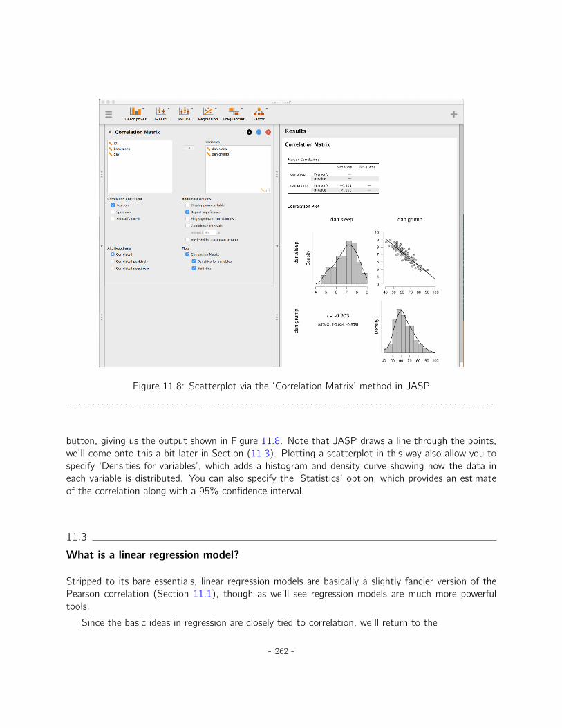
Figure 11.8: Scatterplot via the ‘Correlation Matrix’ method in JASP

. . . . . . . . . . . . . . . . . . . . . . . . . . . . . . . . . . . . . . . . . . . . . . . . . . . . . . . . . . . . . . . . . . . . . . . . . . . . . . . . . . . . . . . . . . . .

button, giving us the output shown in Figure 11.8. Note that JASP draws a line through the points,we’ll come onto this a bit later in Section (11.3). Plotting a scatterplot in this way also allow you tospecify ‘Densities for variables’, which adds a histogram and density curve showing how the data ineach variable is distributed. You can also specify the ‘Statistics’ option, which provides an estimateof the correlation along with a 95% confidence interval.

11.3

What is a linear regression model?

Stripped to its bare essentials, linear regression models are basically a slightly fancier version of thePearson correlation (Section 11.1), though as we’ll see regression models are much more powerfultools.

Since the basic ideas in regression are closely tied to correlation, we’ll return to the

- 262 -

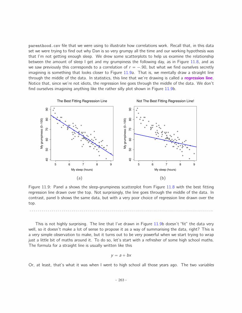
parenthood.csv file that we were using to illustrate how correlations work. Recall that, in this dataset we were trying to find out why Dan is so very grumpy all the time and our working hypothesis wasthat I’m not getting enough sleep. We drew some scatterplots to help us examine the relationshipbetween the amount of sleep I get and my grumpiness the following day, as in Figure 11.8, and aswe saw previously this corresponds to a correlation of r “ ´.90, but what we find ourselves secretlyimagining is something that looks closer to Figure 11.9a. That is, we mentally draw a straight linethrough the middle of the data. In statistics, this line that we’re drawing is called a regression line.Notice that, since we’re not idiots, the regression line goes through the middle of the data. We don’tfind ourselves imagining anything like the rather silly plot shown in Figure 11.9b.

5 6 7 8 9

40

50

60

70

80

90

The Best Fitting Regression Line

My sleep (hours)

My g

rum

pin

ess (

0−

10

0)

5 6 7 8 9

40

50

60

70

80

90

Not The Best Fitting Regression Line!

My sleep (hours)

My g

rum

pin

ess (

0−

10

0)

(a) (b)

Figure 11.9: Panel a shows the sleep-grumpiness scatterplot from Figure 11.8 with the best fittingregression line drawn over the top. Not surprisingly, the line goes through the middle of the data. Incontrast, panel b shows the same data, but with a very poor choice of regression line drawn over thetop.

. . . . . . . . . . . . . . . . . . . . . . . . . . . . . . . . . . . . . . . . . . . . . . . . . . . . . . . . . . . . . . . . . . . . . . . . . . . . . . . . . . . . . . . . . . . .

This is not highly surprising. The line that I’ve drawn in Figure 11.9b doesn’t “fit” the data verywell, so it doesn’t make a lot of sense to propose it as a way of summarising the data, right? This isa very simple observation to make, but it turns out to be very powerful when we start trying to wrapjust a little bit of maths around it. To do so, let’s start with a refresher of some high school maths.The formula for a straight line is usually written like this

y “ a ` bx

Or, at least, that’s what it was when I went to high school all those years ago. The two variables

- 263 -

are x and y , and we have two coefficients, a and b.2 The coefficient a represents the y -interceptof the line, and coefficient b represents the slope of the line. Digging further back into our decayingmemories of high school (sorry, for some of us high school was a long time ago), we remember thatthe intercept is interpreted as “the value of y that you get when x “ 0”. Similarly, a slope of b meansthat if you increase the x-value by 1 unit, then the y -value goes up by b units, and a negative slopemeans that the y -value would go down rather than up. Ah yes, it’s all coming back to me now. Nowthat we’ve remembered that it should come as no surprise to discover that we use the exact sameformula for a regression line. If Y is the outcome variable (the DV) and X is the predictor variable(the IV), then the formula that describes our regression is written like this

Yi “ b0 ` b1Xi

Hmm. Looks like the same formula, but there’s some extra frilly bits in this version. Let’s make surewe understand them. Firstly, notice that I’ve written Xi and Yi rather than just plain old X and Y .This is because we want to remember that we’re dealing with actual data. In this equation, Xi is thevalue of predictor variable for the ith observation (i.e., the number of hours of sleep that I got on dayi of my little study), and Yi is the corresponding value of the outcome variable (i.e., my grumpinesson that day). And although I haven’t said so explicitly in the equation, what we’re assuming is thatthis formula works for all observations in the data set (i.e., for all i). Secondly, notice that I wroteYi and not Yi . This is because we want to make the distinction between the actual data Yi , and theestimate Yi (i.e., the prediction that our regression line is making). Thirdly, I changed the letters usedto describe the coefficients from a and b to b0 and b1. That’s just the way that statisticians like torefer to the coefficients in a regression model. I’ve no idea why they chose b, but that’s what theydid. In any case b0 always refers to the intercept term, and b1 refers to the slope.

Excellent, excellent. Next, I can’t help but notice that, regardless of whether we’re talking aboutthe good regression line or the bad one, the data don’t fall perfectly on the line. Or, to say it anotherway, the data Yi are not identical to the predictions of the regression model Yi . Since statisticianslove to attach letters, names and numbers to everything, let’s refer to the difference between themodel prediction and that actual data point as a residual, and we’ll refer to it as εi .3 Written usingmathematics, the residuals are defined as

εi “ Yi ´ Yi

which in turn means that we can write down the complete linear regression model as

Yi “ b0 ` b1Xi ` εi

- 264 -

5 6 7 8 9

40

50

60

70

80

90

Regression Line Close to the Data

My sleep (hours)

My g

rum

pin

ess (

0−

10

0)

5 6 7 8 9

40

50

60

70

80

90

Regression Line Distant from the Data

My sleep (hours)

My g

rum

pin

ess (

0−

10

0)

(a) (b)

Figure 11.10: A depiction of the residuals associated with the best fitting regression line (panel a),and the residuals associated with a poor regression line (panel b). The residuals are much smaller forthe good regression line. Again, this is no surprise given that the good line is the one that goes rightthrough the middle of the data.

. . . . . . . . . . . . . . . . . . . . . . . . . . . . . . . . . . . . . . . . . . . . . . . . . . . . . . . . . . . . . . . . . . . . . . . . . . . . . . . . . . . . . . . . . . . .

11.4

Estimating a linear regression model

Okay, now let’s redraw our pictures but this time I’ll add some lines to show the size of the residualfor all observations. When the regression line is good, our residuals (the lengths of the solid blacklines) all look pretty small, as shown in Figure 11.10a, but when the regression line is a bad one theresiduals are a lot larger, as you can see from looking at Figure 11.10b. Hmm. Maybe what we “want”in a regression model is small residuals. Yes, that does seem to make sense. In fact, I think I’ll goso far as to say that the “best fitting” regression line is the one that has the smallest residuals. Or,better yet, since statisticians seem to like to take squares of everything why not say that:

The estimated regression coefficients, b0 and b1, are those that minimise the sum of thesquared residuals, which we could either write as

ř

ipYi ´ Yiq2 or as

ř

i εi2.

Yes, yes that sounds even better. And since I’ve indented it like that, it probably means that this is the2Also sometimes written as y “ mx ` b where m is the slope coefficient and b is the intercept (constant) coefficient.3The ε symbol is the Greek letter epsilon. It’s traditional to use εi or ei to denote a residual.

- 265 -

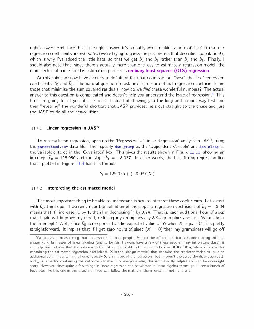
right answer. And since this is the right answer, it’s probably worth making a note of the fact that ourregression coefficients are estimates (we’re trying to guess the parameters that describe a population!),which is why I’ve added the little hats, so that we get b0 and b1 rather than b0 and b1. Finally, Ishould also note that, since there’s actually more than one way to estimate a regression model, themore technical name for this estimation process is ordinary least squares (OLS) regression.

At this point, we now have a concrete definition for what counts as our “best” choice of regressioncoefficients, b0 and b1. The natural question to ask next is, if our optimal regression coefficients arethose that minimise the sum squared residuals, how do we find these wonderful numbers? The actualanswer to this question is complicated and doesn’t help you understand the logic of regression.4 Thistime I’m going to let you off the hook. Instead of showing you the long and tedious way first andthen “revealing” the wonderful shortcut that JASP provides, let’s cut straight to the chase and justuse JASP to do all the heavy lifting.

11.4.1 Linear regression in JASP

To run my linear regression, open up the ‘Regression’ - ‘Linear Regression’ analysis in JASP, usingthe parenthood.csv data file. Then specify dan.grump as the ‘Dependent Variable’ and dan.sleep asthe variable entered in the ‘Covariates’ box. This gives the results shown in Figure 11.11, showing anintercept b0 “ 125.956 and the slope b1 “ ´8.937. In other words, the best-fitting regression linethat I plotted in Figure 11.9 has this formula:

Yi “ 125.956` p´8.937 Xiq

11.4.2 Interpreting the estimated model

The most important thing to be able to understand is how to interpret these coefficients. Let’s startwith b1, the slope. If we remember the definition of the slope, a regression coefficient of b1 “ ´8.94

means that if I increase Xi by 1, then I’m decreasing Yi by 8.94. That is, each additional hour of sleepthat I gain will improve my mood, reducing my grumpiness by 8.94 grumpiness points. What aboutthe intercept? Well, since b0 corresponds to “the expected value of Yi when Xi equals 0”, it’s prettystraightforward. It implies that if I get zero hours of sleep (Xi “ 0) then my grumpiness will go off

4Or at least, I’m assuming that it doesn’t help most people. But on the off chance that someone reading this is aproper kung fu master of linear algebra (and to be fair, I always have a few of these people in my intro stats class), itwill help you to know that the solution to the estimation problem turns out to be b “ pX1Xq´1X1y, where b is a vectorcontaining the estimated regression coefficients, X is the “design matrix” that contains the predictor variables (plus anadditional column containing all ones; strictly X is a matrix of the regressors, but I haven’t discussed the distinction yet),and y is a vector containing the outcome variable. For everyone else, this isn’t exactly helpful and can be downrightscary. However, since quite a few things in linear regression can be written in linear algebra terms, you’ll see a bunch offootnotes like this one in this chapter. If you can follow the maths in them, great. If not, ignore it.

- 266 -

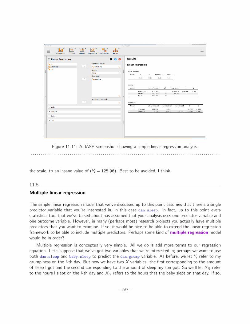
Figure 11.11: A JASP screenshot showing a simple linear regression analysis.

. . . . . . . . . . . . . . . . . . . . . . . . . . . . . . . . . . . . . . . . . . . . . . . . . . . . . . . . . . . . . . . . . . . . . . . . . . . . . . . . . . . . . . . . . . . .

the scale, to an insane value of (Yi “ 125.96). Best to be avoided, I think.

11.5

Multiple linear regression

The simple linear regression model that we’ve discussed up to this point assumes that there’s a singlepredictor variable that you’re interested in, in this case dan.sleep. In fact, up to this point everystatistical tool that we’ve talked about has assumed that your analysis uses one predictor variable andone outcome variable. However, in many (perhaps most) research projects you actually have multiplepredictors that you want to examine. If so, it would be nice to be able to extend the linear regressionframework to be able to include multiple predictors. Perhaps some kind of multiple regression modelwould be in order?

Multiple regression is conceptually very simple. All we do is add more terms to our regressionequation. Let’s suppose that we’ve got two variables that we’re interested in; perhaps we want to useboth dan.sleep and baby.sleep to predict the dan.grump variable. As before, we let Yi refer to mygrumpiness on the i-th day. But now we have two X variables: the first corresponding to the amountof sleep I got and the second corresponding to the amount of sleep my son got. So we’ll let Xi1 referto the hours I slept on the i-th day and Xi2 refers to the hours that the baby slept on that day. If so,

- 267 -

then we can write our regression model like this:

Yi “ b0 ` b1Xi1 ` b2Xi2 ` εi

As before, εi is the residual associated with the i-th observation, εi “ Yi ´ Yi . In this model, we nowhave three coefficients that need to be estimated: b0 is the intercept, b1 is the coefficient associatedwith my sleep, and b2 is the coefficient associated with my son’s sleep. However, although the numberof coefficients that need to be estimated has changed, the basic idea of how the estimation worksis unchanged: our estimated coefficients b0, b1 and b2 are those that minimise the sum squaredresiduals.

11.5.1 Doing it in JASP

Multiple regression in JASP is no different to simple regression. All we have to do is add addi-tional variables to the ‘Covariates’ box in JASP. For example, if we want to use both dan.sleep andbaby.sleep as predictors in our attempt to explain why I’m so grumpy, then move baby.sleep acrossinto the ‘Covariates’ box alongside dan.sleep. By default, JASP assumes that the model shouldinclude an intercept. The coefficients we get this time are:

(Intercept) dan.sleep baby.sleep125.966 -8.950 0.011

The coefficient associated with dan.sleep is quite large, suggesting that every hour of sleep I losemakes me a lot grumpier. However, the coefficient for baby.sleep is very small, suggesting that itdoesn’t really matter how much sleep my son gets. What matters as far as my grumpiness goes ishow much sleep I get. To get a sense of what this multiple regression model looks like, Figure 11.12shows a 3D plot that plots all three variables, along with the regression model itself.

11.5.2 Formula for the general case

The equation that I gave above shows you what a multiple regression model looks like when youinclude two predictors. Not surprisingly, then, if you want more than two predictors all you have todo is add more X terms and more b coefficients. In other words, if you have K predictor variablesin the model then the regression equation looks like this

Yi “ b0 `

˜

Kÿ

k“1

bkXik

¸

` εi

- 268 -

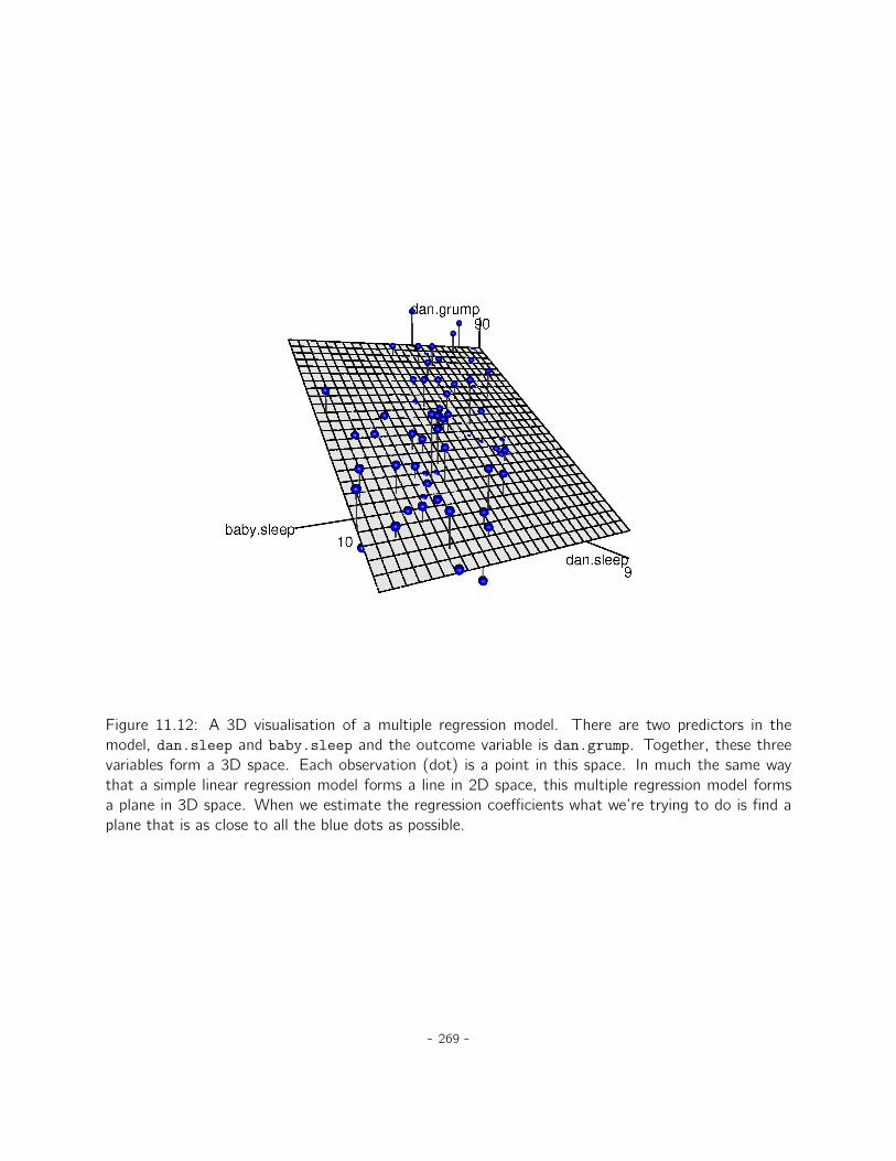
Figure 11.12: A 3D visualisation of a multiple regression model. There are two predictors in themodel, dan.sleep and baby.sleep and the outcome variable is dan.grump. Together, these threevariables form a 3D space. Each observation (dot) is a point in this space. In much the same waythat a simple linear regression model forms a line in 2D space, this multiple regression model formsa plane in 3D space. When we estimate the regression coefficients what we’re trying to do is find aplane that is as close to all the blue dots as possible.

- 269 -

11.6

Quantifying the fit of the regression model

So we now know how to estimate the coefficients of a linear regression model. The problem is, wedon’t yet know if this regression model is any good. For example, the regression model that weconstructed in section 11.4.1 claims that every hour of sleep will improve my mood by quite a lot, butit might just be rubbish. Remember, the regression model only produces a prediction Yi about whatmy mood is like, but my actual mood is Yi . If these two are very close, then the regression model hasdone a good job. If they are very different, then it has done a bad job.

11.6.1 The R2 value

Once again, let’s wrap a little bit of mathematics around this. Firstly, we’ve got the sum of thesquared residuals

SSres “ÿ

i

pYi ´ Yiq2

which we would hope to be pretty small. Specifically, what we’d like is for it to be very small incomparison to the total variability in the outcome variable

SStot “ÿ

i

pYi ´ Y q2

While we’re here, let’s calculate these values ourselves, not by hand though. I have constructed a JASPfile called parenthood_rsquared.jasp, which you can open from the book’s data folder. You’ll noticethat this data file has 5 variables; two of them are the original dan.sleep and dan.grump variables thatwe’ve already been using. The other three are calculated variables:

1. Y.pred is the predicted value of grumpiness using the regression equation. It is calculated usingthe formula ‘125.97 + (-8.94 * dan.sleep)’.

2. resid is a measure of the residual error εi “ Yi ´ Yi , which represents the difference between ourpredicted value of grumpiness and our actual value of grumpiness. It is calculated using the formula‘dan.grump - Y.pred’.

3. sq.resid is the square of the residual, and is calculated using the formula ‘resid2’.

Since SSres is the sum of these squared residuals, we can use JASP to find the sum of the sq.residcolumn. Simply click ‘Descriptives’ - ‘Descriptive Statistics’ and move sq.resid to the ‘Variables’ box.You’ll then need to select ‘Sum’ from the ‘Statistics’ options below. This should give you a value of‘1838.714’.

Wonderful. A big number that doesn’t mean very much. Still, let’s forge boldly onwards anywayand calculate the total sum of squares as well. That’s also pretty simple. Let’s calculate SStotsimilarly. This time, you’ll need to create a new computed column. Click the “+” symbol to start. For

- 270 -

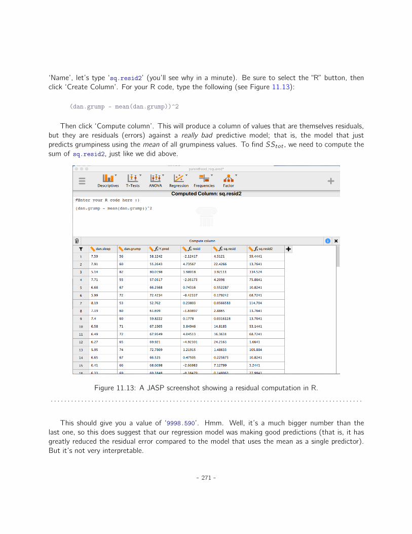
‘Name’, let’s type ‘sq.resid2’ (you’ll see why in a minute). Be sure to select the “R” button, thenclick ‘Create Column’. For your R code, type the following (see Figure 11.13):

(dan.grump - mean(dan.grump))^2

Then click ‘Compute column’. This will produce a column of values that are themselves residuals,but they are residuals (errors) against a really bad predictive model; that is, the model that justpredicts grumpiness using the mean of all grumpiness values. To find SStot , we need to compute thesum of sq.resid2, just like we did above.

Figure 11.13: A JASP screenshot showing a residual computation in R.

. . . . . . . . . . . . . . . . . . . . . . . . . . . . . . . . . . . . . . . . . . . . . . . . . . . . . . . . . . . . . . . . . . . . . . . . . . . . . . . . . . . . . . . . . . . .

This should give you a value of ‘9998.590’. Hmm. Well, it’s a much bigger number than thelast one, so this does suggest that our regression model was making good predictions (that is, it hasgreatly reduced the residual error compared to the model that uses the mean as a single predictor).But it’s not very interpretable.

- 271 -

Perhaps we can fix this. What we’d like to do is to convert these two fairly meaningless numbersinto one number. A nice, interpretable number, which for no particular reason we’ll call R2. What wewould like is for the value of R2 to be equal to 1 if the regression model makes no errors in predictingthe data. In other words, if it turns out that the residual errors are zero. That is, if SSres “ 0 thenwe expect R2 “ 1. Similarly, if the model is completely useless, we would like R2 to be equal to 0.What do I mean by “useless”? Tempting as it is to demand that the regression model move out of thehouse, cut its hair and get a real job, I’m probably going to have to pick a more practical definition.In this case, all I mean is that the residual sum of squares is no smaller than the total sum of squares,SSres “ SStot . Wait, why don’t we do exactly that? The formula that provides us with our R2 valueis pretty simple to write down,

R2 “ 1´SSresSStot

and equally simple to calculate by hand:

R2 “ 1´SSresSStot

“ 1´1838.714

9998.590

“ 1´ 0.1839

“ 0.8161.

The R2 value, sometimes called the coefficient of determination5 has a simple interpretation: it isthe proportion of the variance in the outcome variable that can be accounted for by the predictor. So,in this case the fact that we have obtained R2 “ .8161 means that the predictor (dan.sleep) explains81.61% of the variance in the outcome (dan.grump).

Naturally, you don’t actually need to do all these computations by hand if you want to obtain theR2 value for your regression model. It turns out that JASP gives you this by default! Take a look atFigure 11.11 again; notice that in the top table labeled ‘Model Summary’, the value of R2 is alreadythere!

11.6.2 The relationship between regression and correlation

At this point we can revisit my earlier claim that regression, in this very simple form that I’vediscussed so far, is basically the same thing as a correlation. Previously, we used the symbol r todenote a Pearson correlation. Might there be some relationship between the value of the correlationcoefficient r and the R2 value from linear regression? Of course there is: the squared correlation r2 isidentical to the R2 value for a linear regression with only a single predictor. In other words, running a

5And by “sometimes” I mean “almost never”. In practice everyone just calls it “R-squared”.

- 272 -

Pearson correlation is more or less equivalent to running a linear regression model that uses only onepredictor variable.

11.6.3 The adjusted R2 value

One final thing to point out before moving on. It’s quite common for people to report a slightlydifferent measure of model performance, known as “adjusted R2”. The motivation behind calculatingthe adjusted R2 value is the observation that adding more predictors into the model will always causethe R2 value to increase (or at least not decrease).

The adjusted R2 value introduces a slight change to the calculation, as follows. For a regressionmodel with K predictors, fit to a data set containing N observations, the adjusted R2 is:

adj. R2 “ 1´

ˆ

SSresSStot

ˆN ´ 1

N ´K ´ 1

˙

This adjustment is an attempt to take the degrees of freedom into account. The big advantage ofthe adjusted R2 value is that when you add more predictors to the model, the adjusted R2 value willonly increase if the new variables improve the model performance more than you’d expect by chance.The big disadvantage is that the adjusted R2 value can’t be interpreted in the elegant way that R2

can. R2 has a simple interpretation as the proportion of variance in the outcome variable that isexplained by the regression model. To my knowledge, no equivalent interpretation exists for adjustedR2.

An obvious question then is whether you should report R2 or adjusted R2. This is probably amatter of personal preference. If you care more about interpretability, then R2 is better. If you caremore about correcting for bias, then adjusted R2 is probably better. Speaking just for myself, I preferR2. My feeling is that it’s more important to be able to interpret your measure of model performance.Besides, as we’ll see in Section 11.7, if you’re worried that the improvement in R2 that you get byadding a predictor is just due to chance and not because it’s a better model, well we’ve got hypothesistests for that.

11.7

Hypothesis tests for regression models

So far we’ve talked about what a regression model is, how the coefficients of a regression modelare estimated, and how we quantify the performance of the model (the last of these, incidentally, isbasically our measure of effect size). The next thing we need to talk about is hypothesis tests. Thereare two different (but related) kinds of hypothesis tests that we need to talk about: those in which wetest whether the regression model as a whole is performing significantly better than a null model, and

- 273 -

those in which we test whether a particular regression coefficient is significantly different from zero.

11.7.1 Testing the model as a whole

Okay, suppose you’ve estimated your regression model. The first hypothesis test you might try isthe null hypothesis that there is no relationship between the predictors and the outcome, and thealternative hypothesis that the data are distributed in exactly the way that the regression modelpredicts.

Formally, our “null model” corresponds to the fairly trivial “regression” model in which we include 0predictors and only include the intercept term b0:

H0 : Yi “ b0 ` εi

If our regression model has K predictors, the “alternative model” is described using the usual formulafor a multiple regression model:

H1 : Yi “ b0 `

˜

Kÿ

k“1

bkXik

¸

` εi

How can we test these two hypotheses against each other? The trick is to understand that it’spossible to divide up the total variance SStot into the sum of the residual variance SSres and theregression model variance SSmod . I’ll skip over the technicalities, since we’ll get to that later whenwe look at ANOVA in Chapter 12. But just note that

SSmod “ SStot ´ SSres

And we can convert the sums of squares into mean squares by dividing by the degrees of freedom.

MSmod “SSmoddfmod

MSres “SSresdfres

So, how many degrees of freedom do we have? As you might expect the df associated with themodel is closely tied to the number of predictors that we’ve included. In fact, it turns out thatdfmod “ K. For the residuals the total degrees of freedom is dfres “ N ´K ´ 1.

- 274 -

Now that we’ve got our mean square values we can calculate an F -statistic like this

F “MSmodMSres

and the degrees of freedom associated with this are K and N ´K ´ 1.

We’ll see much more of the F statistic in Chapter 12, but for now just know that we can interpretlarge F values as indicating that the null hypothesis is performing poorly in comparison to the alternativehypothesis. In a moment I’ll show you how to do the test in JASP the easy way, but first let’s have alook at the tests for the individual regression coefficients.

11.7.2 Tests for individual coefficients

The F -test that we’ve just introduced is useful for checking that the model as a whole is performingbetter than chance. If your regression model doesn’t produce a significant result for the F -test thenyou probably don’t have a very good regression model (or, quite possibly, you don’t have very gooddata). However, while failing this test is a pretty strong indicator that the model has problems, passingthe test (i.e., rejecting the null) doesn’t imply that the model is good! Why is that, you might bewondering? The answer to that can be found by looking at the coefficients for the multiple regressionmodel we have already looked at in section 11.5 above, where the coefficients we got were:

(Intercept) dan.sleep baby.sleep125.966 -8.950 0.011

I can’t help but notice that the estimated regression coefficient for the baby.sleep variable is tiny(0.011), relative to the value that we get for dan.sleep (-8.950). Given that these two variables areabsolutely on the same scale (they’re both measured in “hours slept”), I find this illuminating. In fact,I’m beginning to suspect that it’s really only the amount of sleep that I get that matters in order topredict my grumpiness.

We can re-use a hypothesis test that we discussed earlier, the t-test. The test that we’re interestedin has a null hypothesis that the true regression coefficient is zero (b “ 0), which is to be tested againstthe alternative hypothesis that it isn’t (b ‰ 0). That is:

H0 : b “ 0

H1 : b ‰ 0

How can we test this? Well, if the central limit theorem is kind to us we might be able to guessthat the sampling distribution of b, the estimated regression coefficient, is a normal distribution withmean centred on b. What that would mean is that if the null hypothesis were true, then the samplingdistribution of b has mean zero and unknown standard deviation. Assuming that we can come up witha good estimate for the standard error of the regression coefficient, sepbq, then we’re in luck. That’sexactly the situation for which we introduced the one-sample t-test way back in Chapter 10. So let’s

- 275 -

define a t-statistic like this

t “b

sepbq

I’ll skip over the reasons why, but our degrees of freedom in this case are df “ N´K´1. Irritatingly,the estimate of the standard error of the regression coefficient, sepbq, is not as easy to calculateas the standard error of the mean that we used for the simpler t-tests in Chapter 10. In fact, theformula is somewhat ugly, and not terribly helpful to look at.6 For our purposes it’s sufficient topoint out that the standard error of the estimated regression coefficient depends on both the predictorand outcome variables, and it is somewhat sensitive to violations of the homogeneity of varianceassumption (discussed shortly).

In any case, this t-statistic can be interpreted in the same way as the t-statistics that we discussedin Chapter 10. Assuming that you have a two-sided alternative (i.e., you don’t really care if b ą 0 orb ă 0), then it’s the extreme values of t (i.e., a lot less than zero or a lot greater than zero) thatsuggest that you should reject the null hypothesis.

11.7.3 Running the hypothesis tests in JASP

To compute all of the statistics that we have talked about so far, all you need to do is make surethe relevant options are checked in JASP and then run the regression. Fortunately, these options areusually selected by default. As you can see in Figure 11.14, we get a whole bunch of useful output.

The ‘Coefficients’ at the bottom of the JASP analysis results shown in 11.14 provides the coeffi-cients of the regression model. Each row in this table refers to one of the coefficients in the regressionmodel. The first row is the intercept term, and the later ones look at each of the predictors. Thecolumns give you all of the relevant information. The first column (labeled ‘Unstandardized’) is theactual estimate of b (e.g., 125.966 for the intercept, and -8.950 for the dan.sleep predictor). Thesecond column is the standard error estimate σb. The third column provides a ‘Standardized’ regres-sion coefficient; more about this in Section 11.8. The fourth column gives you the t-statistic, and it’sworth noticing that in this table t “ b{sepbq every time. Finally, the last column gives you the actualp-value for each of these tests.7

The only thing that the coefficients table itself doesn’t list is the degrees of freedom used in the t-test, which is always N´K´1 and is listed in the table in the middle of the output, labelled ‘ANOVA’.We can see from this table that the model performs significantly better than you’d expect by chance(F p2, 97q “ 215.238, p ă .001), which isn’t all that surprising: the R2 “ .816 value indicate thatthe regression model accounts for 81.6% of the variability in the outcome measure. However, when

6For advanced readers only. The vector of residuals is ε “ y´Xb. For K predictors plus the intercept, the estimatedresidual variance is σ2

“ ε1ε{pN ´ K ´ 1q. The estimated covariance matrix of the coefficients is σ2pX1Xq´1, the main

diagonal of which is sepbq, our estimated standard errors.7Note that, although JASP has done multiple tests here, it hasn’t done any sort of correction for multiple comparisons.

These are standard one-sample t-tests with a two-sided alternative. If you want to make corrections for multiple tests,you need to do that yourself.

- 276 -

Figure 11.14: A JASP screenshot showing a multiple linear regression analysis, including relevanthypothesis tests.

. . . . . . . . . . . . . . . . . . . . . . . . . . . . . . . . . . . . . . . . . . . . . . . . . . . . . . . . . . . . . . . . . . . . . . . . . . . . . . . . . . . . . . . . . . . .

we look back up at the t-tests for each of the individual coefficients, we can see that the baby.sleepvariable seems to have no significant effect. All the work in this model is being done by the dan.sleepvariable. Taken together, these results suggest that this regression model is actually the wrong modelfor the data. You’d probably be better off dropping the baby.sleep predictor entirely. In other words,the simple regression model that we started with is likely the better model.

11.8

Regarding regression coefficients

Before moving on to discuss the assumptions underlying linear regression and what you can do tocheck if they’re being met, there’s two more topics I want to briefly discuss, both of which relate tothe regression coefficients. The first thing to talk about is calculating confidence intervals for thecoefficients. After that, I’ll discuss the somewhat murky question of how to determine which predictoris most important.

- 277 -

11.8.1 Confidence intervals for the coefficients

Like any population parameter, the regression coefficients b cannot be estimated with complete pre-cision from a sample of data; that’s part of why we need hypothesis tests. Given this, it’s quite usefulto be able to report confidence intervals that capture our uncertainty about the true value of b. Thisis especially useful when the research question focuses heavily on an attempt to find out how stronglyvariable X is related to variable Y , since in those situations the interest is primarily in the regressionweight b.

Fortunately, confidence intervals for the regression weights can be constructed in the usual fashion

CIpbq “ b ˘`

tcr it ˆ sepbq˘

where sepbq is the standard error of the regression coefficient, and tcr it is the relevant critical valueof the appropriate t distribution. For instance, if it’s a 95% confidence interval that we want, thenthe critical value is the 97.5th quantile of a t distribution with N ´ K ´ 1 degrees of freedom. Inother words, this is basically the same approach to calculating confidence intervals that we’ve usedthroughout.

In JASP we can display confidence intervals by selecting ‘Confidence intervals’ from the ‘Statistics’menu in our regression model dialog. The default is 95% CI, but we could easily choose somethingdifferent, say 99%, if that is what we decided on.

11.8.2 Calculating standardised regression coefficients

One more thing that you might want to do is to calculate “standardised” regression coefficients,often denoted β. The rationale behind standardised coefficients goes like this. In a lot of situations,your variables are on fundamentally different scales. Suppose, for example, my regression model aimsto predict people’s IQ scores using their educational attainment (number of years of education) andtheir income as predictors. Obviously, educational attainment and income are not on the same scales.The number of years of schooling might only vary by 10s of years, whereas income can vary by 10,000sof dollars (or more). The units of measurement have a big influence on the regression coefficients. Theb coefficients only make sense when interpreted in light of the units, both of the predictor variables andthe outcome variable. This makes it very difficult to compare the coefficients of different predictors.Yet there are situations where you really do want to make comparisons between different coefficients.Specifically, you might want some kind of standard measure of which predictors have the strongestrelationship to the outcome. This is what standardised coefficients aim to do.

The basic idea is quite simple; the standardised coefficients are the coefficients that you would

- 278 -

have obtained if you’d converted all the variables to z-scores before running the regression.8 The ideahere is that, by converting all the predictors to z-scores, they all go into the regression on the samescale, thereby removing the problem of having variables on different scales. Regardless of what theoriginal variables were, a β value of 1 means that an increase in the predictor of 1 standard deviationwill produce a corresponding 1 standard deviation increase in the outcome variable. Therefore, ifvariable A has a larger absolute value of β than variable B, it is deemed to have a stronger relationshipwith the outcome. Or at least that’s the idea. It’s worth being a little cautious here, since this doesrely very heavily on the assumption that “a 1 standard deviation change” is fundamentally the samekind of thing for all variables. It’s not always obvious that this is true.

Leaving aside the interpretation issues, let’s look at how it’s calculated. What you could do isstandardise all the variables yourself and then run a regression, but there’s a much simpler way todo it. As it turns out, the β coefficient for a predictor X and outcome Y has a very simple formula,namely

βX “ bX ˆσXσY

where σX is the standard deviation of the predictor, and σY is the standard deviation of the outcomevariable Y . This makes matters a lot simpler.

To make things even simpler, JASP computes the β coefficients by default, as you can see the thirdcolumn of the ‘Coefficients’ table in Figure 11.14. This clearly shows that the dan.sleep variable hasa much stronger effect than the baby.sleep variable. However, this is a perfect example of a situationwhere it would probably make sense to use the original coefficients b rather than the standardisedcoefficients β. After all, my sleep and the baby’s sleep are already on the same scale: number of hoursslept. Why complicate matters by converting these to z-scores?

11.9

Assumptions of regression

The linear regression model that I’ve been discussing relies on several assumptions. In Section 11.10we’ll talk a lot more about how to check that these assumptions are being met, but first let’s have alook at each of them.

• Normality. Like many of the models in statistics, basic simple or multiple linear regression relieson an assumption of normality. Specifically, it assumes that the residuals are normally distributed.It’s actually okay if the predictors X and the outcome Y are non-normal, so long as the residualsε are normal. See Section 11.10.3.

8Strictly, you standardise all the regressors. That is, every “thing” that has a regression coefficient associated withit in the model. For the regression models that I’ve talked about so far, each predictor variable maps onto exactly oneregressor, and vice versa. However, that’s not actually true in general and we’ll see some examples of this in Chapter 13.But, for now we don’t need to care too much about this distinction.

- 279 -

• Linearity. A pretty fundamental assumption of the linear regression model is that the relationshipbetween X and Y actually is linear! Regardless of whether it’s a simple regression or a multipleregression, we assume that the relationships involved are linear.

• Homogeneity of variance. Strictly speaking, the regression model assumes that each residualεi is generated from a normal distribution with mean 0, and (more importantly for the currentpurposes) with a standard deviation σ that is the same for every single residual. In practice, it’simpossible to test the assumption that every residual is identically distributed. Instead, what wecare about is that the standard deviation of the residual is the same for all values of Y , and (ifwe’re being especially paranoid) all values of every predictor X in the model.

• Uncorrelated predictors. The idea here is that, in a multiple regression model, you don’t wantyour predictors to be too strongly correlated with each other. This isn’t “technically” an as-sumption of the regression model, but in practice it’s required. Predictors that are too stronglycorrelated with each other (referred to as “collinearity”) can cause problems when evaluating themodel.

• Residuals are independent of each other. This is really just a “catch all” assumption, to theeffect that “there’s nothing else funny going on in the residuals”. If there is something weird(e.g., the residuals all depend heavily on some other unmeasured variable) going on, it mightscrew things up.

• No “bad” outliers. Again, not actually a technical assumption of the model (or rather, it’s sortof implied by all the others), but there is an implicit assumption that your regression modelisn’t being too strongly influenced by one or two anomalous data points because this raisesquestions about the adequacy of the model and the trustworthiness of the data in some cases.See Section 11.10.2.

11.10

Model checking

The main focus of this section is regression diagnostics, a term that refers to the art of checkingthat the assumptions of your regression model have been met, figuring out how to fix the model if theassumptions are violated, and generally to check that nothing “funny” is going on. I refer to this as the“art” of model checking with good reason. It’s not easy, and while there are a lot of fairly standardisedtools that you can use to diagnose and maybe even cure the problems that ail your model (if thereare any, that is!), you really do need to exercise a certain amount of judgement when doing this. It’seasy to get lost in all the details of checking this thing or that thing, and it’s quite exhausting to tryto remember what all the different things are. This has the very nasty side effect that a lot of peopleget frustrated when trying to learn all the tools, so instead they decide not to do any model checking.This is a bit of a worry!

- 280 -

In this section I describe several different things you can do to check that your regression model isdoing what it’s supposed to. It doesn’t cover the full space of things you could do, but it’s still muchmore detailed than what I see a lot of people doing in practice, and even I don’t usually cover all ofthis in my intro stats class either. However, I do think it’s important that you get a sense of whattools are at your disposal, so I’ll try to introduce a bunch of them here. Finally, I should note thatthis section draws quite heavily from the Fox and Weisberg (2011) text, the book associated with thecar package that is used to conduct regression analysis in R. The car package is notable for providingsome excellent tools for regression diagnostics, and the book itself talks about them in an admirablyclear fashion. I don’t want to sound too gushy about it, but I do think that Fox et al. (2011) is wellworth reading, even if some of the advanced diagnostic techniques are only available in R and notJASP.

11.10.1 Three kinds of residuals

The majority of regression diagnostics revolve around looking at the residuals, and by now you’veprobably formed a sufficiently pessimistic theory of statistics to be able to guess that, precisely becauseof the fact that we care a lot about the residuals, there are several different kinds of residual thatwe might consider. In particular, the following three kinds of residuals are referred to in this section:“ordinary residuals”, “standardised residuals”, and “Studentised residuals”. There is a fourth kind thatyou’ll see referred to in some of the Figures, and that’s the “Pearson residual”. However, for the modelsthat we’re talking about in this chapter the Pearson residual is identical to the ordinary residual.

The first and simplest kind of residuals that we care about are ordinary residuals. These are theactual raw residuals that I’ve been talking about throughout this chapter so far. The ordinary residualis just the difference between the fitted value Yi and the observed value Yi . I’ve been using the notationεi to refer to the i-th ordinary residual, and darn it, I’m going to stick to it. With this in mind, wehave the very simple equation

εi “ Yi ´ Yi

This is of course what we saw earlier, and unless I specifically refer to some other kind of residual,this is the one I’m talking about. So there’s nothing new here. I just wanted to repeat myself. Onedrawback to using ordinary residuals is that they’re always on a different scale, depending on what theoutcome variable is and how good the regression model is. That is, unless you’ve decided to run aregression model without an intercept term, the ordinary residuals will have mean 0 but the variance isdifferent for every regression. In a lot of contexts, especially where you’re only interested in the patternof the residuals and not their actual values, it’s convenient to estimate the standardised residuals,which are normalised in such a way as to have standard deviation 1.

The way we calculate these is to divide the ordinary residual by an estimate of the (population)standard deviation of these residuals. For technical reasons, mumble mumble, the formula for this

- 281 -

isε1i “

εi

σ?

1´ hi

where σ in this context is the estimated population standard deviation of the ordinary residuals, andhi is the “hat value” of the ith observation. I haven’t explained hat values to you yet (but have nofear,a it’s coming shortly), so this won’t make a lot of sense. For now, it’s enough to interpret thestandardised residuals as if we’d converted the ordinary residuals to z-scores. In fact, that is moreor less the truth, it’s just that we’re being a bit fancier.

aOr have no hope, as the case may be.

The third kind of residuals are Studentised residuals (also called “jackknifed residuals”) and they’reeven fancier than standardised residuals. Again, the idea is to take the ordinary residual and divide itby some quantity in order to estimate some standardised notion of the residual.

The formula for doing the calculations this time is subtly different

ε˚i “εi

σpíq?

1´ hi

Notice that our estimate of the standard deviation here is written σpíq. What this corresponds to isthe estimate of the residual standard deviation that you would have obtained if you just deleted theith observation from the data set. This sounds like the sort of thing that would be a nightmare tocalculate, since it seems to be saying that you have to run N new regression models (even a moderncomputer might grumble a bit at that, especially if you’ve got a large data set). Fortunately,some terribly clever person has shown that this standard deviation estimate is actually given by thefollowing equation:

σpíq “ σ

d

N ´K ´ 1´ ε1i2

N ´K ´ 2

Isn’t that a pip?

Before moving on, I should point out that you don’t often need to obtain these residuals yourself,even though they are at the heart of almost all regression diagnostics. Most of the time the variousoptions that provide the diagnostics, or assumption checks, will take care of these calculations foryou. Even so, it’s always nice to know how to actually get hold of these things yourself in case youever need to do something non-standard.

11.10.2 Three kinds of anomalous data

One danger that you can run into with linear regression models is that your analysis might bedisproportionately sensitive to a smallish number of “unusual” or “anomalous” observations. I discussed

- 282 -

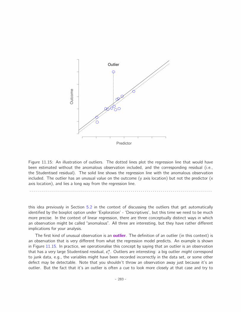
Predictor

Ou

tco

me

Outlier

Figure 11.15: An illustration of outliers. The dotted lines plot the regression line that would havebeen estimated without the anomalous observation included, and the corresponding residual (i.e.,the Studentised residual). The solid line shows the regression line with the anomalous observationincluded. The outlier has an unusual value on the outcome (y axis location) but not the predictor (xaxis location), and lies a long way from the regression line.

. . . . . . . . . . . . . . . . . . . . . . . . . . . . . . . . . . . . . . . . . . . . . . . . . . . . . . . . . . . . . . . . . . . . . . . . . . . . . . . . . . . . . . . . . . . .

this idea previously in Section 5.2 in the context of discussing the outliers that get automaticallyidentified by the boxplot option under ‘Exploration’ - ‘Descriptives’, but this time we need to be muchmore precise. In the context of linear regression, there are three conceptually distinct ways in whichan observation might be called “anomalous”. All three are interesting, but they have rather differentimplications for your analysis.

The first kind of unusual observation is an outlier. The definition of an outlier (in this context) isan observation that is very different from what the regression model predicts. An example is shownin Figure 11.15. In practice, we operationalise this concept by saying that an outlier is an observationthat has a very large Studentised residual, ε˚i . Outliers are interesting: a big outlier might correspondto junk data, e.g., the variables might have been recorded incorrectly in the data set, or some otherdefect may be detectable. Note that you shouldn’t throw an observation away just because it’s anoutlier. But the fact that it’s an outlier is often a cue to look more closely at that case and try to

- 283 -

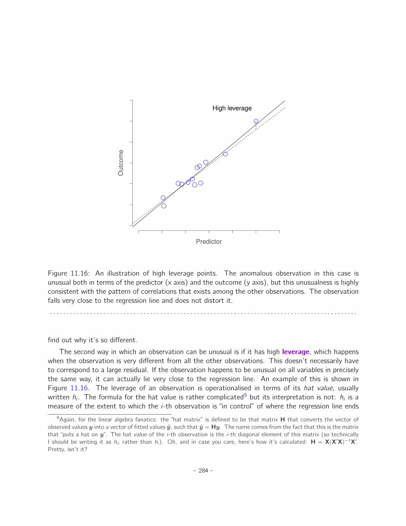
Predictor

Ou

tco

me

High leverage

Figure 11.16: An illustration of high leverage points. The anomalous observation in this case isunusual both in terms of the predictor (x axis) and the outcome (y axis), but this unusualness is highlyconsistent with the pattern of correlations that exists among the other observations. The observationfalls very close to the regression line and does not distort it.

. . . . . . . . . . . . . . . . . . . . . . . . . . . . . . . . . . . . . . . . . . . . . . . . . . . . . . . . . . . . . . . . . . . . . . . . . . . . . . . . . . . . . . . . . . . .

find out why it’s so different.

The second way in which an observation can be unusual is if it has high leverage, which happenswhen the observation is very different from all the other observations. This doesn’t necessarily haveto correspond to a large residual. If the observation happens to be unusual on all variables in preciselythe same way, it can actually lie very close to the regression line. An example of this is shown inFigure 11.16. The leverage of an observation is operationalised in terms of its hat value, usuallywritten hi . The formula for the hat value is rather complicated9 but its interpretation is not: hi is ameasure of the extent to which the i-th observation is “in control” of where the regression line ends

9Again, for the linear algebra fanatics: the “hat matrix” is defined to be that matrix H that converts the vector ofobserved values y into a vector of fitted values y, such that y “ Hy. The name comes from the fact that this is the matrixthat “puts a hat on y”. The hat value of the i-th observation is the i-th diagonal element of this matrix (so technicallyI should be writing it as hi i rather than hi). Oh, and in case you care, here’s how it’s calculated: H “ XpX1Xq´1X1.Pretty, isn’t it?

- 284 -

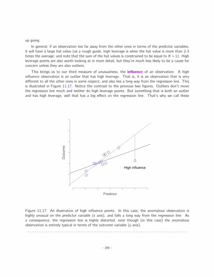
up going.

In general, if an observation lies far away from the other ones in terms of the predictor variables,it will have a large hat value (as a rough guide, high leverage is when the hat value is more than 2-3times the average; and note that the sum of the hat values is constrained to be equal to K`1). Highleverage points are also worth looking at in more detail, but they’re much less likely to be a cause forconcern unless they are also outliers.

This brings us to our third measure of unusualness, the influence of an observation. A highinfluence observation is an outlier that has high leverage. That is, it is an observation that is verydifferent to all the other ones in some respect, and also lies a long way from the regression line. Thisis illustrated in Figure 11.17. Notice the contrast to the previous two figures. Outliers don’t movethe regression line much and neither do high leverage points. But something that is both an outlierand has high leverage, well that has a big effect on the regression line. That’s why we call these

Predictor

Ou

tco

me

High influence

Figure 11.17: An illustration of high influence points. In this case, the anomalous observation ishighly unusual on the predictor variable (x axis), and falls a long way from the regression line. Asa consequence, the regression line is highly distorted, even though (in this case) the anomalousobservation is entirely typical in terms of the outcome variable (y axis).

. . . . . . . . . . . . . . . . . . . . . . . . . . . . . . . . . . . . . . . . . . . . . . . . . . . . . . . . . . . . . . . . . . . . . . . . . . . . . . . . . . . . . . . . . . . .

- 285 -

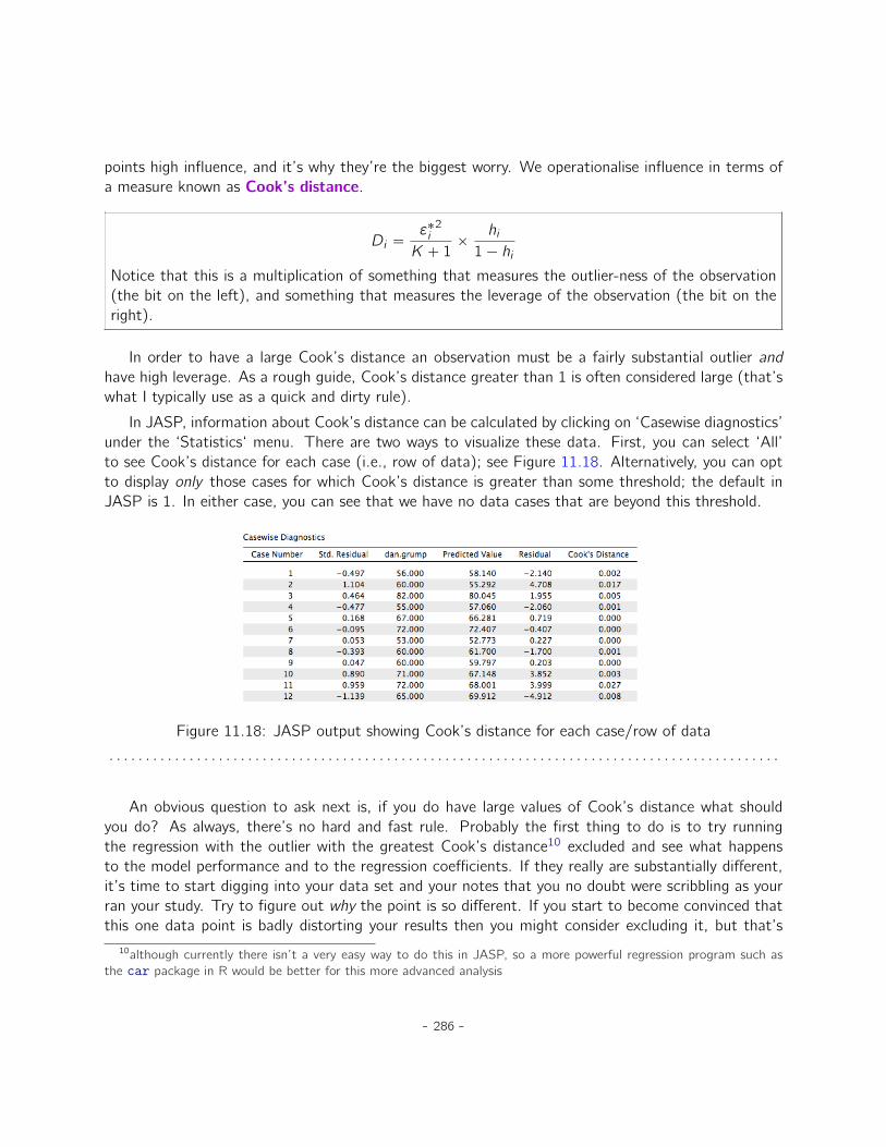
points high influence, and it’s why they’re the biggest worry. We operationalise influence in terms ofa measure known as Cook’s distance.

Di “ε˚i

2

K ` 1ˆ

hi1´ hi

Notice that this is a multiplication of something that measures the outlier-ness of the observation(the bit on the left), and something that measures the leverage of the observation (the bit on theright).

In order to have a large Cook’s distance an observation must be a fairly substantial outlier andhave high leverage. As a rough guide, Cook’s distance greater than 1 is often considered large (that’swhat I typically use as a quick and dirty rule).

In JASP, information about Cook’s distance can be calculated by clicking on ‘Casewise diagnostics’under the ‘Statistics‘ menu. There are two ways to visualize these data. First, you can select ‘All’to see Cook’s distance for each case (i.e., row of data); see Figure 11.18. Alternatively, you can optto display only those cases for which Cook’s distance is greater than some threshold; the default inJASP is 1. In either case, you can see that we have no data cases that are beyond this threshold.

Figure 11.18: JASP output showing Cook’s distance for each case/row of data

. . . . . . . . . . . . . . . . . . . . . . . . . . . . . . . . . . . . . . . . . . . . . . . . . . . . . . . . . . . . . . . . . . . . . . . . . . . . . . . . . . . . . . . . . . . .

An obvious question to ask next is, if you do have large values of Cook’s distance what shouldyou do? As always, there’s no hard and fast rule. Probably the first thing to do is to try runningthe regression with the outlier with the greatest Cook’s distance10 excluded and see what happensto the model performance and to the regression coefficients. If they really are substantially different,it’s time to start digging into your data set and your notes that you no doubt were scribbling as yourran your study. Try to figure out why the point is so different. If you start to become convinced thatthis one data point is badly distorting your results then you might consider excluding it, but that’s

10although currently there isn’t a very easy way to do this in JASP, so a more powerful regression program such asthe car package in R would be better for this more advanced analysis

- 286 -

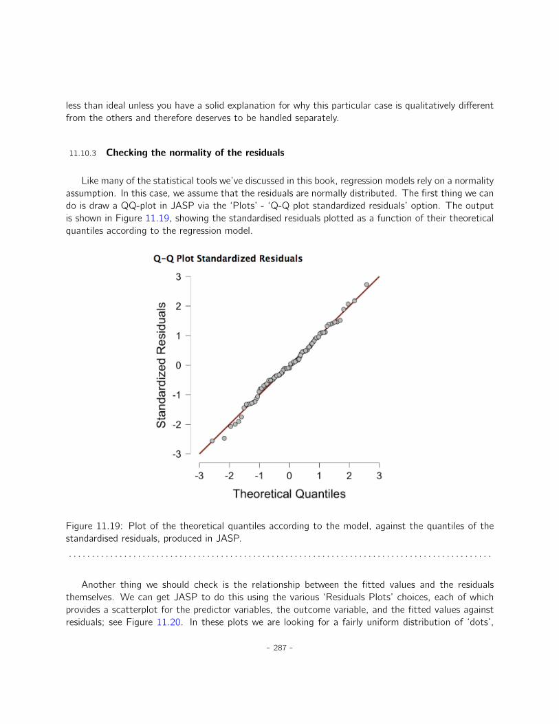
less than ideal unless you have a solid explanation for why this particular case is qualitatively differentfrom the others and therefore deserves to be handled separately.

11.10.3 Checking the normality of the residuals

Like many of the statistical tools we’ve discussed in this book, regression models rely on a normalityassumption. In this case, we assume that the residuals are normally distributed. The first thing we cando is draw a QQ-plot in JASP via the ‘Plots’ - ‘Q-Q plot standardized residuals’ option. The outputis shown in Figure 11.19, showing the standardised residuals plotted as a function of their theoreticalquantiles according to the regression model.

Figure 11.19: Plot of the theoretical quantiles according to the model, against the quantiles of thestandardised residuals, produced in JASP.

. . . . . . . . . . . . . . . . . . . . . . . . . . . . . . . . . . . . . . . . . . . . . . . . . . . . . . . . . . . . . . . . . . . . . . . . . . . . . . . . . . . . . . . . . . . .

Another thing we should check is the relationship between the fitted values and the residualsthemselves. We can get JASP to do this using the various ‘Residuals Plots’ choices, each of whichprovides a scatterplot for the predictor variables, the outcome variable, and the fitted values againstresiduals; see Figure 11.20. In these plots we are looking for a fairly uniform distribution of ‘dots’,

- 287 -

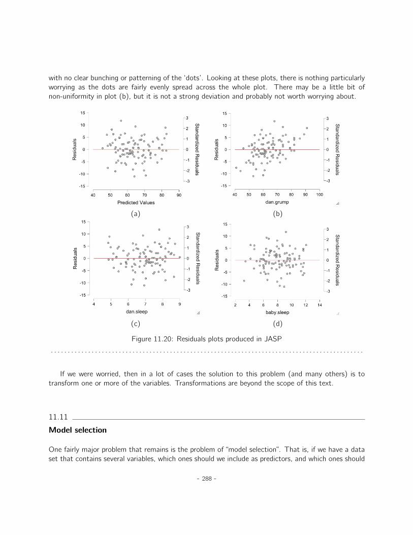
with no clear bunching or patterning of the ‘dots’. Looking at these plots, there is nothing particularlyworrying as the dots are fairly evenly spread across the whole plot. There may be a little bit ofnon-uniformity in plot (b), but it is not a strong deviation and probably not worth worrying about.

(a) (b)

(c) (d)

Figure 11.20: Residuals plots produced in JASP

. . . . . . . . . . . . . . . . . . . . . . . . . . . . . . . . . . . . . . . . . . . . . . . . . . . . . . . . . . . . . . . . . . . . . . . . . . . . . . . . . . . . . . . . . . . .

If we were worried, then in a lot of cases the solution to this problem (and many others) is totransform one or more of the variables. Transformations are beyond the scope of this text.

11.11

Model selection

One fairly major problem that remains is the problem of “model selection”. That is, if we have a dataset that contains several variables, which ones should we include as predictors, and which ones should

- 288 -

we not include? In other words, we have a problem of variable selection. In general, model selection isa complex business but it’s made somewhat simpler if we restrict ourselves to the problem of choosinga subset of the variables that ought to be included in the model. Nevertheless, I’m not going to trycovering even this reduced topic in a lot of detail. Instead, I’ll talk about two broad principles thatyou need to think about, and then discuss one concrete tool to help you select a subset of variablesto include in your model. First, the two principles:

• It’s nice to have an actual substantive basis for your choices. That is, in a lot of situations youthe researcher have good reasons to pick out a smallish number of possible regression modelsthat are of theoretical interest. These models will have a sensible interpretation in the contextof your field. Never discount the importance of this. Statistics serves the scientific process, notthe other way around.

• To the extent that your choices rely on statistical inference, there is a trade off between simplicityand goodness of fit. As you add more predictors to the model you make it more complex. Eachpredictor adds a new free parameter (i.e., a new regression coefficient), and each new parameterincreases the model’s capacity to “absorb” random variations. So the goodness of fit (e.g., R2)continues to rise, sometimes trivially or by chance, as you add more predictors no matter what.If you want your model to be able to generalise well to new observations you need to avoidthrowing in too many variables.

This latter principle is often referred to as Ockham’s razor and is often summarised in terms of thefollowing pithy saying: do not multiply entities beyond necessity. In this context, it means don’t chuckin a bunch of largely irrelevant predictors just to boost your R2. Hmm. Yeah, the original was better.

In any case, what we need is an actual mathematical criterion that will implement the qualitativeprinciple behind Ockham’s razor in the context of selecting a regression model. As it turns out thereare several possibilities. The one that I’ll talk about is the Akaike information criterion (AIC; Akaike1974); currently, it is not part of JASP’s standard output, but it is quite easy to compute with themodel fit data that JASP does produce.

In the context of a linear regression model, the AIC for a model that has n observations and Kpredictor variables (not including the intercept) can be computeda as

AIC “ n lnpSSresq ` 2K

aStrictly speaking, this formula is not completely correct. Akaike’s original definition was in terms of somethingcalled a maximum likelihood estimate for the model, and as such, there are some other terms that appear in thecomputation. However, many of them don’t depend on the model, and given that the purpose of the AIC is tocompare models, these terms will be present in all models and will mathematically “wash out”. Thus, I am presentinga ‘bare bones’ version of the formula that is sufficient for our purposes.

Here’s the basic principle behind using AIC for model comparison: the smaller the AIC value, thebetter the model performance. If we ignore the low level details it’s fairly obvious what the AIC does.

- 289 -

On the left we have a term that decreases as the model predictions get better; on the right we havea term that increases as the model complexity increases. The best model is the one that both fitsthe data well (small SSres , left hand side) and uses as few predictors as possible (small K, right handside). In short, this is a simple mathematical implementation of Ockham’s razor.

Let’s demonstrate how AIC can be used to compare the two regression models we have computedin this chapter. Consider first the regression model with only one predictor: dan.sleep (see Figure11.11). In this model, we have n “ 100 observations, K “ 1 predictor, and SSres “ 1838.714. Thus,

AIC1 “ n lnpSSresq ` 2K

“ 100 lnp1838.714q ` 2p1q

“ 753.68

Now consider the second model using two predictors: dan.sleep and baby.sleep (see Figure11.14). In this model, we have n “ 100 observations, K “ 2 predictors, and SSres “ 1838.685. Thisgives us

AIC2 “ n lnpSSresq ` 2K

“ 100 lnp1838.685q ` 2p2q

“ 755.68.

Since AIC1 ă AIC2, this tells us that Model 1 is the better fit, which confirms our intuitions.Adding baby.sleep doesn’t add much to the model fit, but it increases model complexity. AIC balancesthese two requirements; the penalty for adding an additional parameter is not outweighed by the meagerimprovement in model fit.

11.12

Summary

• Want to know how strong the relationship is between two variables? Calculate a correlation(Section 11.1).

• Drawing scatterplots (Section 11.2).

• Basic ideas in linear regression and how regression models are estimated (Sections 11.3 and11.4).

• Multiple linear regression (Section 11.5).

• Measuring the overall performance of a regression model using R2 (Section 11.6).

- 290 -

• Hypothesis tests for regression models (Section 11.7)

• Calculating confidence intervals for regression coefficients and standardised coefficients (Sec-tion 11.8).

• The assumptions of regression (Section 11.9) and how to check them (Section 11.10).

• Selecting a regression model (Section 11.11).

- 291 -

- 292 -

12. Comparing several means (one-way ANOVA)

This chapter introduces one of the most widely used tools in psychological statistics, known as “theanalysis of variance”, but usually referred to as ANOVA. The basic technique was developed by SirRonald Fisher in the early 20th century and it is to him that we owe the rather unfortunate terminology.The term ANOVA is a little misleading, in two respects. Firstly, although the name of the techniquerefers to variances, ANOVA is concerned with investigating differences in means. Secondly, there areseveral different things out there that are all referred to as ANOVAs, some of which have only a verytenuous connection to one another. Later on in the book we’ll encounter a range of different ANOVAmethods that apply in quite different situations, but for the purposes of this chapter we’ll only considerthe simplest form of ANOVA, in which we have several different groups of observations, and we’reinterested in finding out whether those groups differ in terms of some outcome variable of interest.This is the question that is addressed by a one-way ANOVA.

The structure of this chapter is as follows: in Section 12.1 I’ll introduce a fictitious data set thatwe’ll use as a running example throughout the chapter. After introducing the data, I’ll describe themechanics of how a one-way ANOVA actually works (Section 12.2) and then focus on how you can runone in JASP (Section 12.3). These two sections are the core of the chapter. The remainder of thechapter discusses a range of important topics that inevitably arise when running an ANOVA, namelyhow to calculate effect sizes (Section 12.4), post hoc tests and corrections for multiple comparisons(Section 12.5) and the assumptions that ANOVA relies upon (Section 12.6). We’ll also talk abouthow to check those assumptions and some of the things you can do if the assumptions are violated(Sections 12.6.1 to 12.7). Then we’ll cover repeated measures ANOVA in Sections 12.8 and 12.9. Atthe end of the chapter we’ll talk a little about the relationship between ANOVA and other statisticaltools (Section 12.10).

12.1

An illustrative data set

Suppose you’ve become involved in a clinical trial in which you are testing a new antidepressant drugcalled Joyzepam. In order to construct a fair test of the drug’s effectiveness, the study involves three

- 293 -

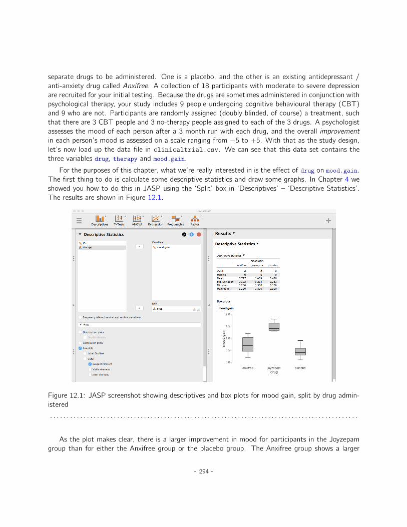
separate drugs to be administered. One is a placebo, and the other is an existing antidepressant /anti-anxiety drug called Anxifree. A collection of 18 participants with moderate to severe depressionare recruited for your initial testing. Because the drugs are sometimes administered in conjunction withpsychological therapy, your study includes 9 people undergoing cognitive behavioural therapy (CBT)and 9 who are not. Participants are randomly assigned (doubly blinded, of course) a treatment, suchthat there are 3 CBT people and 3 no-therapy people assigned to each of the 3 drugs. A psychologistassesses the mood of each person after a 3 month run with each drug, and the overall improvementin each person’s mood is assessed on a scale ranging from ´5 to `5. With that as the study design,let’s now load up the data file in clinicaltrial.csv. We can see that this data set contains thethree variables drug, therapy and mood.gain.

For the purposes of this chapter, what we’re really interested in is the effect of drug on mood.gain.The first thing to do is calculate some descriptive statistics and draw some graphs. In Chapter 4 weshowed you how to do this in JASP using the ‘Split’ box in ‘Descriptives’ – ‘Descriptive Statistics’.The results are shown in Figure 12.1.

Figure 12.1: JASP screenshot showing descriptives and box plots for mood gain, split by drug admin-istered

. . . . . . . . . . . . . . . . . . . . . . . . . . . . . . . . . . . . . . . . . . . . . . . . . . . . . . . . . . . . . . . . . . . . . . . . . . . . . . . . . . . . . . . . . . . .

As the plot makes clear, there is a larger improvement in mood for participants in the Joyzepamgroup than for either the Anxifree group or the placebo group. The Anxifree group shows a larger

- 294 -

mood gain than the control group, but the difference isn’t as large. The question that we want toanswer is are these difference “real”, or are they just due to chance?

12.2

How ANOVA works

In order to answer the question posed by our clinical trial data we’re going to run a one-way ANOVA.I’m going to start by showing you how to do it the hard way, building the statistical tool from theground up and showing you how you could do it if you didn’t have access to any of the cool built-inANOVA functions in JASP. And I hope you’ll read it carefully, try to do it the long way once or twiceto make sure you really understand how ANOVA works, and then once you’ve grasped the conceptnever ever do it this way again.

The experimental design that I described in the previous section strongly suggests that we’reinterested in comparing the average mood change for the three different drugs. In that sense, we’retalking about an analysis similar to the t-test (Chapter 10) but involving more than two groups. Ifwe let µP denote the population mean for the mood change induced by the placebo, and let µA andµJ denote the corresponding means for our two drugs, Anxifree and Joyzepam, then the (somewhatpessimistic) null hypothesis that we want to test is that all three population means are identical. Thatis, neither of the two drugs is any more effective than a placebo. We can write out this null hypothesisas:

H0 : it is true that µP “ µA “ µJ

As a consequence, our alternative hypothesis is that at least one of the three different treatmentsis different from the others. It’s a bit tricky to write this mathematically, because (as we’ll discuss)there are quite a few different ways in which the null hypothesis can be false. So for now we’ll justwrite the alternative hypothesis like this:

H1 : it is not true that µP “ µA “ µJ

This null hypothesis is a lot trickier to test than any of the ones we’ve seen previously. How shall wedo it? A sensible guess would be to “do an ANOVA”, since that’s the title of the chapter, but it’snot particularly clear why an “analysis of variances” will help us learn anything useful about the means.In fact, this is one of the biggest conceptual difficulties that people have when first encounteringANOVA. To see how this works, I find it most helpful to start by talking about variances. In fact,what I’m going to do is start by playing some mathematical games with the formula that describesthe variance. That is, we’ll start out by playing around with variances and it will turn out that thisgives us a useful tool for investigating means.

- 295 -

12.2.1 Two formulas for the variance of Y

First, let’s start by introducing some notation. We’ll use G to refer to the total number of groups.For our data set there are three drugs, so there are G “ 3 groups. Next, we’ll use N to refer to thetotal sample size; there are a total of N “ 18 people in our data set. Similarly, let’s use Nk to denotethe number of people in the k-th group. In our fake clinical trial, the sample size is Nk “ 6 for allthree groups.1 Finally, we’ll use Y to denote the outcome variable. In our case, Y refers to moodchange. Specifically, we’ll use Yik to refer to the mood change experienced by the i-th member of thek-th group. Similarly, we’ll use Y to be the average mood change, taken across all 18 people in theexperiment, and Yk to refer to the average mood change experienced by the 6 people in group k .

Now that we’ve got our notation sorted out we can start writing down formulas. To start with, let’srecall the formula for the variance that we used in Section 4.2, way back in those kinder days whenwe were just doing descriptive statistics. The sample variance of Y is defined as follows

VarpY q “1

N

Gÿ

k“1

Nkÿ

i“1

`

Yik ´ Y˘2

This formula looks pretty much identical to the formula for the variance in Section 4.2. The onlydifference is that this time around I’ve got two summations here: I’m summing over groups (i.e.,values for k) and over the people within the groups (i.e., values for i). This is purely a cosmeticdetail. If I’d instead used the notation Yp to refer to the value of the outcome variable for personp in the sample, then I’d only have a single summation. The only reason that we have a doublesummation here is that I’ve classified people into groups, and then assigned numbers to people withingroups.

A concrete example might be useful here. Let’s consider this table, in which we have a total ofN “ 5 people sorted into G “ 2 groups. Arbitrarily, let’s say that the “cool” people are group 1 andthe “uncool” people are group 2. It turns out that we have three cool people (N1 “ 3) and two uncoolpeople (N2 “ 2)

name person group group num. index in group grumpinessp k i Yik or Yp

Ann 1 cool 1 1 20Ben 2 cool 1 2 55Cat 3 cool 1 3 21Dan 4 uncool 2 1 91Egg 5 uncool 2 2 22

1When all groups have the same number of observations, the experimental design is said to be “balanced”. Balanceisn’t such a big deal for one-way ANOVA, which is the topic of this chapter. It becomes more important when you startdoing more complicated ANOVAs.

- 296 -

Notice that I’ve constructed two different labelling schemes here. We have a “person” variable p soit would be perfectly sensible to refer to Yp as the grumpiness of the p-th person in the sample. Forinstance, the table shows that Dan is the fourth so we’d say p “ 4. So, when talking about thegrumpiness Y of this “Dan” person, whoever he might be, we could refer to his grumpiness by sayingthat Yp “ 91, for person p “ 4 that is. However, that’s not the only way we could refer to Dan. Asan alternative we could note that Dan belongs to the “uncool” group (k “ 2), and is in fact the firstperson listed in the uncool group (i “ 1). So it’s equally valid to refer to Dan’s grumpiness by sayingthat Yik “ 91, where k “ 2 and i “ 1.

In other words, each person p corresponds to a unique ik combination, and so the formula that Igave above is actually identical to our original formula for the variance, which would be

VarpY q “1

N

Nÿ

p“1

`

Yp ´ Y˘2

In both formulas, all we’re doing is summing over all of the observations in the sample. Most of thetime we would just use the simpler Yp notation; the equation using Yp is clearly the simpler of thetwo. However, when doing an ANOVA it’s important to keep track of which participants belong inwhich groups, and we need to use the Yik notation to do this.

12.2.2 From variances to sums of squares

Okay, now that we’ve got a good grasp on how the variance is calculated, let’s define somethingcalled the total sum of squares, which is denoted SStot . This is very simple. Instead of averagingthe squared deviations, which is what we do when calculating the variance, we just add them up.

So the formula for the total sum of squares is almost identical to the formula for the variance

SStot “Gÿ

k“1

Nkÿ

i“1

`

Yik ´ Y˘2

When we talk about analysing variances in the context of ANOVA, what we’re really doing is workingwith the total sums of squares rather than the actual variance. One very nice thing about the totalsum of squares is that we can break it up into two different kinds of variation.

- 297 -

First, we can talk about the within-group sum of squares, in which we look to see how differenteach individual person is from their own group mean

SSw “Gÿ

k“1

Nkÿ

i“1

`

Yik ´ Yk˘2

where Yk is a group mean. In our example, Yk would be the average mood change experiencedby those people given the k-th drug. So, instead of comparing individuals to the average of allpeople in the experiment, we’re only comparing them to those people in the the same group. As aconsequence, you’d expect the value of SSw to be smaller than the total sum of squares, becauseit’s completely ignoring any group differences, i.e., whether the drugs will have different effects onpeople’s moods.

Next, we can define a third notion of variation which captures only the differences between groups.We do this by looking at the differences between the group means Yk and grand mean Y .

In order to quantify the extent of this variation, what we do is calculate the between-group sumof squares

SSb “

Gÿ

k“1

Nkÿ

i“1

`

Yk ´ Y˘2

“

Gÿ

k“1

Nk`

Yk ´ Y˘2

It’s not too difficult to show that the total variation among people in the experiment SStot isactually the sum of the differences between the groups SSb and the variation inside the groups SSw .That is,

SSw ` SSb “ SStot

Yay.

Okay, so what have we found out? We’ve discovered that the total variability associated withthe outcome variable (SStot) can be mathematically carved up into the sum of “the variation due tothe differences in the sample means for the different groups” (SSb) plus “all the rest of the variation”(SSw )2. How does that help me find out whether the groups have different population means? Um.Wait. Hold on a second. Now that I think about it, this is exactly what we were looking for. If the nullhypothesis is true then you’d expect all the sample means to be pretty similar to each other, right?And that would imply that you’d expect SSb to be really small, or at least you’d expect it to be a lotsmaller than “the variation associated with everything else”, SSw . Hmm. I detect a hypothesis testcoming on.

2SSw is also referred to in an independent ANOVA as the error variance, or SSerror

- 298 -

group 1 group 2 group 3

Between−group variation

(i.e., differences among group means)

group 1 group 2 group 3

Within−group variation

(i.e., deviations from group means)

(a) (b)

Figure 12.2: Graphical illustration of “between groups” variation (panel a) and “within groups” variation(panel b). On the left the arrows show the differences in the group means. On the right the arrowshighlight the variability within each group.

. . . . . . . . . . . . . . . . . . . . . . . . . . . . . . . . . . . . . . . . . . . . . . . . . . . . . . . . . . . . . . . . . . . . . . . . . . . . . . . . . . . . . . . . . . . .

12.2.3 From sums of squares to the F -test

As we saw in the last section, the qualitative idea behind ANOVA is to compare the two sums ofsquares values SSb and SSw to each other. If the between-group variation SSb is large relative to thewithin-group variation SSw then we have reason to suspect that the population means for the differentgroups aren’t identical to each other. In order to convert this into a workable hypothesis test, there’sa little bit of “fiddling around” needed. What I’ll do is first show you what we do to calculate our teststatistic, the F ratio, and then try to give you a feel for why we do it this way.

In order to convert our SS values into an F -ratio the first thing we need to calculate is the degreesof freedom associated with the SSb and SSw values. As usual, the degrees of freedom correspondsto the number of unique “data points” that contribute to a particular calculation, minus the numberof “constraints” that they need to satisfy. For the within-groups variability what we’re calculating isthe variation of the individual observations (N data points) around the group means (G constraints).In contrast, for the between groups variability we’re interested in the variation of the group means (Gdata points) around the grand mean (1 constraint). Therefore, the degrees of freedom here are:

dfb “ G ´ 1

dfw “ N ´ G

Okay, that seems simple enough. What we do next is convert our summed squares value into a “meansquares” value, which we do by dividing by the degrees of freedom:

MSb “SSbdfb

MSw “SSwdfw

- 299 -

Table 12.1: All of the key quantities involved in an ANOVA organised into a “standard” ANOVAtable. The formulas for all quantities (except the p-value which has a very ugly formula and would benightmarishly hard to calculate without a computer) are shown.

df sum of squares mean squares F -statistic p-value

betweengroups

dfb “ G ´ 1 SSb “Gÿ

k“1

NkpYk ´ Y q2 MSb “

SSbdfb

F “MSbMSw

[complicated]

withingroups

dfw “ N ´ G SSw “Gÿ

k“1

Nkÿ

i“1

pYik ´ Ykq2 MSw “

SSwdfw

- -

. . . . . . . . . . . . . . . . . . . . . . . . . . . . . . . . . . . . . . . . . . . . . . . . . . . . . . . . . . . . . . . . . . . . . . . . . . . . . . . . . . . . . . . . . . . . . . . . . . . . .

Finally, we calculate the F -ratio by dividing the between-groups MS by the within-groups MS:

F “MSbMSw

At a very general level, the intuition behind the F statistic is straightforward. Bigger values of F meansthat the between-groups variation is large relative to the within-groups variation. As a consequence,the larger the value of F the more evidence we have against the null hypothesis. But how large doesF have to be in order to actually reject H0? In order to understand this, you need a slightly deeperunderstanding of what ANOVA is and what the mean squares values actually are.

The next section discusses that in a bit of detail, but for readers that aren’t interested in thedetails of what the test is actually measuring I’ll cut to the chase. In order to complete our hypothesistest we need to know the sampling distribution for F if the null hypothesis is true. Not surprisingly, thesampling distribution for the F statistic under the null hypothesis is an F distribution. If you recall ourdiscussion of the F distribution in Chapter 6, the F distribution has two parameters, correspondingto the two degrees of freedom involved. The first one df1 is the between groups degrees of freedomdfb, and the second one df2 is the within groups degrees of freedom dfw .

A summary of all the key quantities involved in a one-way ANOVA, including the formulas showinghow they are calculated, is shown in Table 12.1.

12.2.4 The model for the data and the meaning of F

At a fundamental level ANOVA is a competition between two different statistical models, H0 andH1. When I described the null and alternative hypotheses at the start of the section, I was a littleimprecise about what these models actually are. I’ll remedy that now, though you probably won’t like

- 300 -

me for doing so. If you recall, our null hypothesis was that all of the group means are identical to oneanother. If so, then a natural way to think about the outcome variable Yik is to describe individualscores in terms of a single population mean µ, plus the deviation from that population mean. Thisdeviation is usually denoted εik and is traditionally called the error or residual associated with thatobservation. Be careful though. Just like we saw with the word “significant”, the word “error” hasa technical meaning in statistics that isn’t quite the same as its everyday English definition. Ineveryday language, “error” implies a mistake of some kind, but in statistics it doesn’t (or at least,not necessarily). With that in mind, the word “residual” is a better term than the word “error”. Instatistics both words mean “leftover variability”, that is “stuff” that the model can’t explain.

In any case, here’s what the null hypothesis looks like when we write it as a statistical model

Yik “ µ` εik

where we make the assumption (discussed later) that the residual values εik are normally distributed,with mean 0 and a standard deviation σ that is the same for all groups. To use the notation thatwe introduced in Chapter 6 we would write this assumption like this

εik „ Normalp0, σ2q

What about the alternative hypothesis, H1? The only difference between the null hypothesisand the alternative hypothesis is that we allow each group to have a different population mean. So,if we let µk denote the population mean for the k-th group in our experiment, then the statisticalmodel corresponding to H1 is

Yik “ µk ` εik

where, once again, we assume that the error terms are normally distributed with mean 0 and standarddeviation σ. That is, the alternative hypothesis also assumes that ε „ Normalp0, σ2q

Okay, now that we’ve described the statistical models underpinning H0 and H1 in more detail,it’s now pretty straightforward to say what the mean square values are measuring, and what thismeans for the interpretation of F . I won’t bore you with the proof of this but it turns out that thewithin-groups mean square, MSw , can be viewed as an estimator (in the technical sense, Chapter 7)of the error variance σ2. The between-groups mean square MSb is also an estimator, but what itestimates is the error variance plus a quantity that depends on the true differences among the groupmeans. If we call this quantity Q, then we can see that the F -statistic is basicallya

F “Q` σ2

σ2

where the true value Q “ 0 if the null hypothesis is true, and Q ą 0 if the alternative hypothesis istrue (e.g., Hays 1994, ch. 10). Therefore, at a bare minimum the F value must be larger than 1 tohave any chance of rejecting the null hypothesis. Note that this doesn’t mean that it’s impossibleto get an F -value less than 1. What it means is that if the null hypothesis is true the sampling

- 301 -

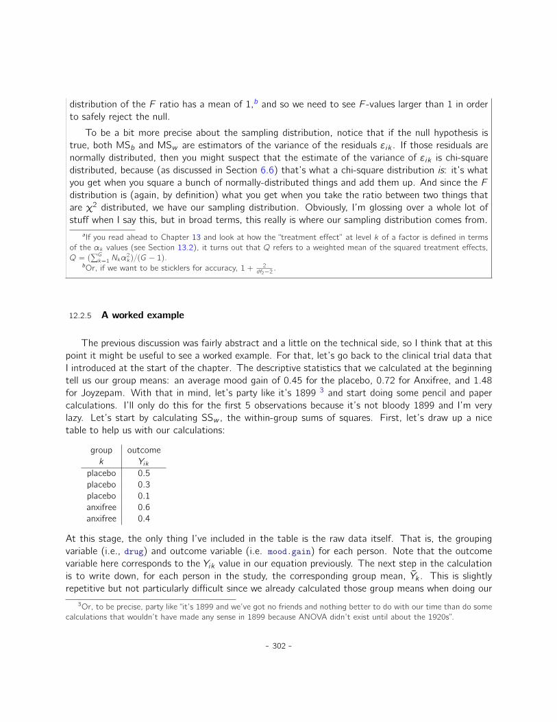
distribution of the F ratio has a mean of 1,b and so we need to see F -values larger than 1 in orderto safely reject the null.

To be a bit more precise about the sampling distribution, notice that if the null hypothesis istrue, both MSb and MSw are estimators of the variance of the residuals εik . If those residuals arenormally distributed, then you might suspect that the estimate of the variance of εik is chi-squaredistributed, because (as discussed in Section 6.6) that’s what a chi-square distribution is: it’s whatyou get when you square a bunch of normally-distributed things and add them up. And since the Fdistribution is (again, by definition) what you get when you take the ratio between two things thatare χ2 distributed, we have our sampling distribution. Obviously, I’m glossing over a whole lot ofstuff when I say this, but in broad terms, this really is where our sampling distribution comes from.

aIf you read ahead to Chapter 13 and look at how the “treatment effect” at level k of a factor is defined in termsof the αk values (see Section 13.2), it turns out that Q refers to a weighted mean of the squared treatment effects,Q “ p

řGk“1 Nkα

2kq{pG ´ 1q.

bOr, if we want to be sticklers for accuracy, 1` 2df2´2

.

12.2.5 A worked example

The previous discussion was fairly abstract and a little on the technical side, so I think that at thispoint it might be useful to see a worked example. For that, let’s go back to the clinical trial data thatI introduced at the start of the chapter. The descriptive statistics that we calculated at the beginningtell us our group means: an average mood gain of 0.45 for the placebo, 0.72 for Anxifree, and 1.48for Joyzepam. With that in mind, let’s party like it’s 1899 3 and start doing some pencil and papercalculations. I’ll only do this for the first 5 observations because it’s not bloody 1899 and I’m verylazy. Let’s start by calculating SSw , the within-group sums of squares. First, let’s draw up a nicetable to help us with our calculations:

group outcomek Yik

placebo 0.5placebo 0.3placebo 0.1anxifree 0.6anxifree 0.4

At this stage, the only thing I’ve included in the table is the raw data itself. That is, the groupingvariable (i.e., drug) and outcome variable (i.e. mood.gain) for each person. Note that the outcomevariable here corresponds to the Yik value in our equation previously. The next step in the calculationis to write down, for each person in the study, the corresponding group mean, Yk . This is slightlyrepetitive but not particularly difficult since we already calculated those group means when doing our

3Or, to be precise, party like “it’s 1899 and we’ve got no friends and nothing better to do with our time than do somecalculations that wouldn’t have made any sense in 1899 because ANOVA didn’t exist until about the 1920s”.

- 302 -

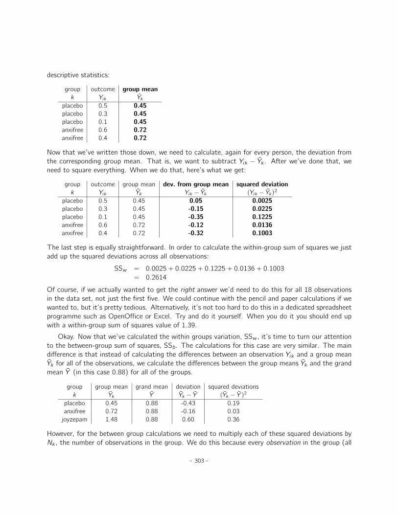
descriptive statistics:

group outcome group meank Yik Yk

placebo 0.5 0.45placebo 0.3 0.45placebo 0.1 0.45anxifree 0.6 0.72anxifree 0.4 0.72

Now that we’ve written those down, we need to calculate, again for every person, the deviation fromthe corresponding group mean. That is, we want to subtract Yik ´ Yk . After we’ve done that, weneed to square everything. When we do that, here’s what we get:

group outcome group mean dev. from group mean squared deviationk Yik Yk Yik ´ Yk pYik ´ Ykq

2

placebo 0.5 0.45 0.05 0.0025placebo 0.3 0.45 -0.15 0.0225placebo 0.1 0.45 -0.35 0.1225anxifree 0.6 0.72 -0.12 0.0136anxifree 0.4 0.72 -0.32 0.1003

The last step is equally straightforward. In order to calculate the within-group sum of squares we justadd up the squared deviations across all observations:

SSw “ 0.0025` 0.0225` 0.1225` 0.0136` 0.1003

“ 0.2614

Of course, if we actually wanted to get the right answer we’d need to do this for all 18 observationsin the data set, not just the first five. We could continue with the pencil and paper calculations if wewanted to, but it’s pretty tedious. Alternatively, it’s not too hard to do this in a dedicated spreadsheetprogramme such as OpenOffice or Excel. Try and do it yourself. When you do it you should end upwith a within-group sum of squares value of 1.39.

Okay. Now that we’ve calculated the within groups variation, SSw , it’s time to turn our attentionto the between-group sum of squares, SSb. The calculations for this case are very similar. The maindifference is that instead of calculating the differences between an observation Yik and a group meanYk for all of the observations, we calculate the differences between the group means Yk and the grandmean Y (in this case 0.88) for all of the groups.

group group mean grand mean deviation squared deviationsk Yk Y Yk ´ Y pYk ´ Y q

2

placebo 0.45 0.88 -0.43 0.19anxifree 0.72 0.88 -0.16 0.03joyzepam 1.48 0.88 0.60 0.36

However, for the between group calculations we need to multiply each of these squared deviations byNk , the number of observations in the group. We do this because every observation in the group (all

- 303 -

Nk of them) is associated with a between group difference. So if there are six people in the placebogroup and the placebo group mean differs from the grand mean by 0.19, then the total between groupvariation associated with these six people is 6ˆ 0.19 “ 1.14. So we have to extend our little table ofcalculations:

group ... squared deviations sample size weighted squared devk ... pYk ´ Y q

2 Nk NkpYk ´ Y q2

placebo ... 0.19 6 1.14anxifree ... 0.03 6 0.18joyzepam ... 0.36 6 2.16

And so now our between group sum of squares is obtained by summing these “weighted squareddeviations” over all three groups in the study:

SSb “ 1.14` 0.18` 2.16

“ 3.48

As you can see, the between group calculations are a lot shorter. Now that we’ve calculated oursums of squares values, SSb and SSw , the rest of the ANOVA is pretty painless. The next step is tocalculate the degrees of freedom. Since we have G “ 3 groups and N “ 18 observations in total ourdegrees of freedom can be calculated by simple subtraction:

dfb “ G ´ 1 “ 2

dfw “ N ´ G “ 15

Next, since we’ve now calculated the values for the sums of squares and the degrees of freedom, forboth the within-groups variability and the between-groups variability, we can obtain the mean squarevalues by dividing one by the other:

MSb “SSbdfb

“3.48

2“ 1.74

MSw “SSwdfw

“1.39

15“ 0.09

We’re almost done. The mean square values can be used to calculate the F -value, which is thetest statistic that we’re interested in. We do this by dividing the between-groups MS value by thewithin-groups MS value.

F “MSbMSw

“1.74

0.09“ 19.3

Woohooo! This is terribly exciting, yes? Now that we have our test statistic, the last step is to findout whether the test itself gives us a significant result. As discussed in Chapter 8 back in the “olddays” what we’d do is open up a statistics textbook or flick to the back section which would actuallyhave a huge lookup table and we would find the threshold F value corresponding to a particular valueof alpha (the null hypothesis rejection region), e.g. 0.05, 0.01 or 0.001, for 2 and 15 degrees offreedom. Doing it this way would give us a threshold F value for an alpha of 0.001 of 11.34. As this

- 304 -

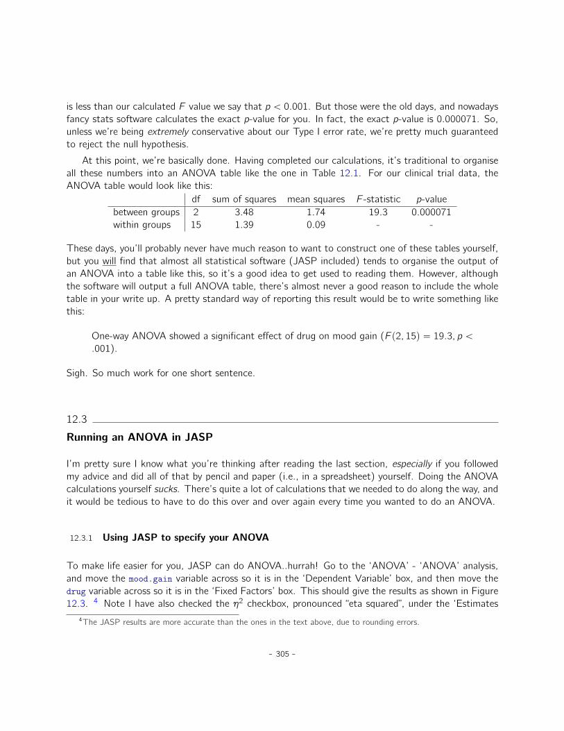
is less than our calculated F value we say that p ă 0.001. But those were the old days, and nowadaysfancy stats software calculates the exact p-value for you. In fact, the exact p-value is 0.000071. So,unless we’re being extremely conservative about our Type I error rate, we’re pretty much guaranteedto reject the null hypothesis.

At this point, we’re basically done. Having completed our calculations, it’s traditional to organiseall these numbers into an ANOVA table like the one in Table 12.1. For our clinical trial data, theANOVA table would look like this:

df sum of squares mean squares F -statistic p-valuebetween groups 2 3.48 1.74 19.3 0.000071within groups 15 1.39 0.09 - -

These days, you’ll probably never have much reason to want to construct one of these tables yourself,but you will find that almost all statistical software (JASP included) tends to organise the output ofan ANOVA into a table like this, so it’s a good idea to get used to reading them. However, althoughthe software will output a full ANOVA table, there’s almost never a good reason to include the wholetable in your write up. A pretty standard way of reporting this result would be to write something likethis:

One-way ANOVA showed a significant effect of drug on mood gain (F p2, 15q “ 19.3, p ă

.001).

Sigh. So much work for one short sentence.

12.3

Running an ANOVA in JASP

I’m pretty sure I know what you’re thinking after reading the last section, especially if you followedmy advice and did all of that by pencil and paper (i.e., in a spreadsheet) yourself. Doing the ANOVAcalculations yourself sucks. There’s quite a lot of calculations that we needed to do along the way, andit would be tedious to have to do this over and over again every time you wanted to do an ANOVA.

12.3.1 Using JASP to specify your ANOVA

To make life easier for you, JASP can do ANOVA..hurrah! Go to the ‘ANOVA’ - ‘ANOVA’ analysis,and move the mood.gain variable across so it is in the ‘Dependent Variable’ box, and then move thedrug variable across so it is in the ‘Fixed Factors’ box. This should give the results as shown in Figure12.3. 4 Note I have also checked the η2 checkbox, pronounced “eta squared”, under the ‘Estimates

4The JASP results are more accurate than the ones in the text above, due to rounding errors.

- 305 -

of effect size’ option that can be found in ‘Additional Options,’ and this is also shown on the resultstable. We will come back to effect sizes a bit later.

Figure 12.3: JASP results table for ANOVA of mood gain by drug administered

. . . . . . . . . . . . . . . . . . . . . . . . . . . . . . . . . . . . . . . . . . . . . . . . . . . . . . . . . . . . . . . . . . . . . . . . . . . . . . . . . . . . . . . . . . . .

The JASP results table shows you the sums of squares values, the degrees of freedom, and acouple of other quantities that we’re not really interested in right now. Notice, however, that JASPdoesn’t use the names “between-group” and “within-group”. Instead, it tries to assign more meaningfulnames. In our particular example, the between groups variance corresponds to the effect that the drughas on the outcome variable, and the within groups variance corresponds to the “leftover” variability soit calls that the residual error. If we compare these numbers to the numbers that I calculated by handin Section 12.2.5, you can see that they’re more or less the same, apart from rounding errors. Thebetween groups sums of squares is SSb “ 3.453, the within groups sums of squares is SSw “ 1.392,and the degrees of freedom are 2 and 15 respectively. We also get the F -value and the p-value and,again, these are more or less the same, give or take rounding errors, to the numbers that we calculatedourselves when doing it the long and tedious way.

12.4

Effect size

There’s a few different ways you could measure the effect size in an ANOVA, but the most commonlyused measures are η2 (eta squared) and partial η2. For a one way analysis of variance they’re identicalto each other, so for the moment I’ll just explain η2. The definition of η2 is actually really simple

η2 “SSbSStot

- 306 -

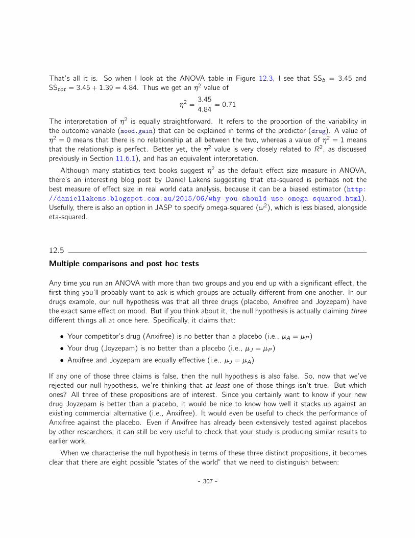
That’s all it is. So when I look at the ANOVA table in Figure 12.3, I see that SSb “ 3.45 andSStot “ 3.45` 1.39 “ 4.84. Thus we get an η2 value of

η2 “3.45

4.84“ 0.71

The interpretation of η2 is equally straightforward. It refers to the proportion of the variability inthe outcome variable (mood.gain) that can be explained in terms of the predictor (drug). A value ofη2 “ 0 means that there is no relationship at all between the two, whereas a value of η2 “ 1 meansthat the relationship is perfect. Better yet, the η2 value is very closely related to R2, as discussedpreviously in Section 11.6.1), and has an equivalent interpretation.

Although many statistics text books suggest η2 as the default effect size measure in ANOVA,there’s an interesting blog post by Daniel Lakens suggesting that eta-squared is perhaps not thebest measure of effect size in real world data analysis, because it can be a biased estimator (http://daniellakens.blogspot.com.au/2015/06/why-you-should-use-omega-squared.html).Usefully, there is also an option in JASP to specify omega-squared (ω2), which is less biased, alongsideeta-squared.

12.5

Multiple comparisons and post hoc tests

Any time you run an ANOVA with more than two groups and you end up with a significant effect, thefirst thing you’ll probably want to ask is which groups are actually different from one another. In ourdrugs example, our null hypothesis was that all three drugs (placebo, Anxifree and Joyzepam) havethe exact same effect on mood. But if you think about it, the null hypothesis is actually claiming threedifferent things all at once here. Specifically, it claims that:

• Your competitor’s drug (Anxifree) is no better than a placebo (i.e., µA “ µP )

• Your drug (Joyzepam) is no better than a placebo (i.e., µJ “ µP )

• Anxifree and Joyzepam are equally effective (i.e., µJ “ µA)

If any one of those three claims is false, then the null hypothesis is also false. So, now that we’verejected our null hypothesis, we’re thinking that at least one of those things isn’t true. But whichones? All three of these propositions are of interest. Since you certainly want to know if your newdrug Joyzepam is better than a placebo, it would be nice to know how well it stacks up against anexisting commercial alternative (i.e., Anxifree). It would even be useful to check the performance ofAnxifree against the placebo. Even if Anxifree has already been extensively tested against placebosby other researchers, it can still be very useful to check that your study is producing similar results toearlier work.

When we characterise the null hypothesis in terms of these three distinct propositions, it becomesclear that there are eight possible “states of the world” that we need to distinguish between:

- 307 -

http://daniellakens.blogspot.com.au/2015/06/why-you-should-use-omega-squared.html

http://daniellakens.blogspot.com.au/2015/06/why-you-should-use-omega-squared.html

possibility: is µP “ µA? is µP “ µJ? is µA “ µJ? which hypothesis?1 X X X null2 X X alternative3 X X alternative4 X alternative5 X X alternative6 X alternative7 X alternative8 alternative

By rejecting the null hypothesis, we’ve decided that we don’t believe that #1 is the true state of theworld. The next question to ask is, which of the other seven possibilities do we think is right? Whenfaced with this situation, its usually helps to look at the data. For instance, if we look at the plotsin Figure 12.1, it’s tempting to conclude that Joyzepam is better than the placebo and better thanAnxifree, but there’s no real difference between Anxifree and the placebo. However, if we want to geta clearer answer about this, it might help to run some tests.

12.5.1 Running “pairwise” t-tests

How might we go about solving our problem? Given that we’ve got three separate pairs of means(placebo versus Anxifree, placebo versus Joyzepam, and Anxifree versus Joyzepam) to compare, whatwe could do is run three separate t-tests and see what happens. This is easy to do in JASP. Go to theANOVA ‘Post Hoc Tests’ options, move the ‘drug’ variable across into the active box on the right.This will immediately produce a neat table showing all the pairwise t-test comparisons amongst thethree levels of the drug variable, as in Figure 12.4.

Figure 12.4: Pairwise t-tests as post hoc comparisons in JASP

. . . . . . . . . . . . . . . . . . . . . . . . . . . . . . . . . . . . . . . . . . . . . . . . . . . . . . . . . . . . . . . . . . . . . . . . . . . . . . . . . . . . . . . . . . . .

- 308 -

12.5.2 Corrections for multiple testing

In the previous section I hinted that there’s a problem with just running lots and lots of t-tests.The concern is that, when running these analyses, what we’re doing is going on a “fishing expedition”.We’re running lots and lots of tests without much theoretical guidance in the hope that some of themcome up significant. This kind of theory-free search for group differences is referred to as post hocanalysis (“post hoc” being Latin for “after this”).5

It’s okay to run post hoc analyses, but a lot of care is required. For instance, the analysis thatI ran in the previous section should be avoided, as each individual t-test is designed to have a 5%Type I error rate (i.e., α “ .05) and I ran three of these tests. Imagine what would have happenedif my ANOVA involved 10 different groups, and I had decided to run 45 “post hoc” t-tests to try tofind out which ones were significantly different from each other, you’d expect 2 or 3 of them to comeup significant by chance alone. As we saw in Chapter 8, the central organising principle behind nullhypothesis testing is that we seek to control our Type I error rate, but now that I’m running lots oft-tests at once in order to determine the source of my ANOVA results, my actual Type I error rateacross this whole family of tests has gotten completely out of control.

The usual solution to this problem is to introduce an adjustment to the p-value, which aims tocontrol the total error rate across the family of tests (see Shaffer 1995). An adjustment of this form,which is usually (but not always) applied because one is doing post hoc analysis, is often referredto as a correction for multiple comparisons, though it is sometimes referred to as “simultaneousinference”. In any case, there are quite a few different ways of doing this adjustment. I’ll discuss afew of them in this section and in Section 13.8, but you should be aware that there are many othermethods out there (see, e.g., Hsu 1996).

12.5.3 Bonferroni corrections

The simplest of these adjustments is called the Bonferroni correction (Dunn 1961), and it’s veryvery simple indeed. Suppose that my post hoc analysis consists of m separate tests, and I want toensure that the total probability of making any Type I errors at all is at most α.6 If so, then theBonferroni correction just says “multiply all your raw p-values by m”. If we let p denote the originalp-value, and let p1j be the corrected value, then the Bonferroni correction tells that:

p1 “ m ˆ p

And therefore, if you’re using the Bonferroni correction, you would reject the null hypothesis if p1 ă α.The logic behind this correction is very straightforward. We’re doing m different tests, so if we arrange

5If you do have some theoretical basis for wanting to investigate some comparisons but not others, it’s a differentstory. In those circumstances you’re not really running “post hoc” analyses at all, you’re making “planned comparisons”.I do talk about this situation later in the book (Section 13.9), but for now I want to keep things simple.

6It’s worth noting in passing that not all adjustment methods try to do this. What I’ve described here is an approachfor controlling “family wise Type I error rate”. However, there are other post hoc tests that seek to control the “falsediscovery rate”, which is a somewhat different thing.

- 309 -

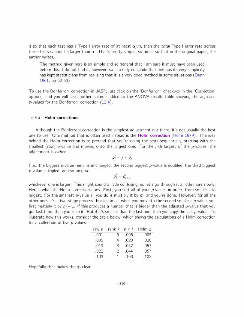
it so that each test has a Type I error rate of at most α{m, then the total Type I error rate acrossthese tests cannot be larger than α. That’s pretty simple, so much so that in the original paper, theauthor writes,

The method given here is so simple and so general that I am sure it must have been usedbefore this. I do not find it, however, so can only conclude that perhaps its very simplicityhas kept statisticians from realizing that it is a very good method in some situations (Dunn1961, pp 52-53)

To use the Bonferroni correction in JASP, just click on the ‘Bonferroni’ checkbox in the ‘Correction’options, and you will see another column added to the ANOVA results table showing the adjustedp-values for the Bonferroni correction (12.4).

12.5.4 Holm corrections

Although the Bonferroni correction is the simplest adjustment out there, it’s not usually the bestone to use. One method that is often used instead is the Holm correction (Holm 1979). The ideabehind the Holm correction is to pretend that you’re doing the tests sequentially, starting with thesmallest (raw) p-value and moving onto the largest one. For the j-th largest of the p-values, theadjustment is either

p1j “ j ˆ pj

(i.e., the biggest p-value remains unchanged, the second biggest p-value is doubled, the third biggestp-value is tripled, and so on), or

p1j “ p1j`1

whichever one is larger. This might sound a little confusing, so let’s go through it a little more slowly.Here’s what the Holm correction does. First, you sort all of your p-values in order, from smallest tolargest. For the smallest p-value all you do is multiply it by m, and you’re done. However, for all theother ones it’s a two-stage process. For instance, when you move to the second smallest p value, youfirst multiply it by m´ 1. If this produces a number that is bigger than the adjusted p-value that yougot last time, then you keep it. But if it’s smaller than the last one, then you copy the last p-value. Toillustrate how this works, consider the table below, which shows the calculations of a Holm correctionfor a collection of five p-values:

raw p rank j p ˆ j Holm p

.001 5 .005 .005

.005 4 .020 .020

.019 3 .057 .057

.022 2 .044 .057

.103 1 .103 .103

Hopefully that makes things clear.

- 310 -

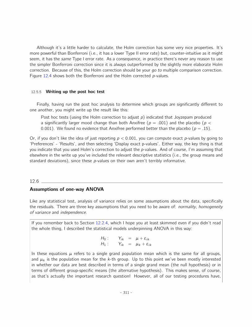
Although it’s a little harder to calculate, the Holm correction has some very nice properties. It’smore powerful than Bonferroni (i.e., it has a lower Type II error rate) but, counter-intuitive as it mightseem, it has the same Type I error rate. As a consequence, in practice there’s never any reason to usethe simpler Bonferroni correction since it is always outperformed by the slightly more elaborate Holmcorrection. Because of this, the Holm correction should be your go to multiple comparison correction.Figure 12.4 shows both the Bonferroni and the Holm corrected p-values.

12.5.5 Writing up the post hoc test

Finally, having run the post hoc analysis to determine which groups are significantly different toone another, you might write up the result like this:

Post hoc tests (using the Holm correction to adjust p) indicated that Joyzepam produceda significantly larger mood change than both Anxifree (p “ .001) and the placebo (p ă0.001). We found no evidence that Anxifree performed better than the placebo (p “ .15).

Or, if you don’t like the idea of just reporting p ă 0.001, you can compute exact p-values by going to‘Preferences’ - ‘Results’, and then selecting ‘Display exact p-values’. Either way, the key thing is thatyou indicate that you used Holm’s correction to adjust the p-values. And of course, I’m assuming thatelsewhere in the write up you’ve included the relevant descriptive statistics (i.e., the group means andstandard deviations), since these p-values on their own aren’t terribly informative.

12.6

Assumptions of one-way ANOVA

Like any statistical test, analysis of variance relies on some assumptions about the data, specificallythe residuals. There are three key assumptions that you need to be aware of: normality, homogeneityof variance and independence.

If you remember back to Section 12.2.4, which I hope you at least skimmed even if you didn’t readthe whole thing, I described the statistical models underpinning ANOVA in this way:

H0 : Yik “ µ` εikH1 : Yik “ µk ` εik

In these equations µ refers to a single grand population mean which is the same for all groups,and µk is the population mean for the k-th group. Up to this point we’ve been mostly interestedin whether our data are best described in terms of a single grand mean (the null hypothesis) or interms of different group-specific means (the alternative hypothesis). This makes sense, of course,as that’s actually the important research question! However, all of our testing procedures have,

- 311 -

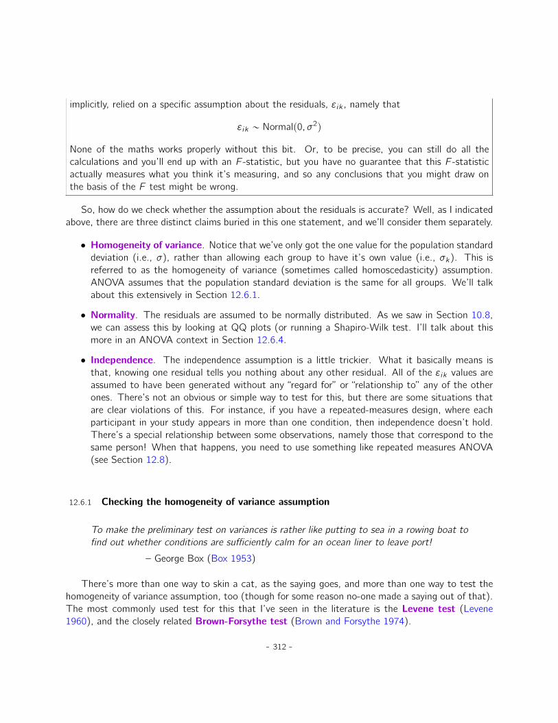
implicitly, relied on a specific assumption about the residuals, εik , namely that

εik „ Normalp0, σ2q

None of the maths works properly without this bit. Or, to be precise, you can still do all thecalculations and you’ll end up with an F -statistic, but you have no guarantee that this F -statisticactually measures what you think it’s measuring, and so any conclusions that you might draw onthe basis of the F test might be wrong.

So, how do we check whether the assumption about the residuals is accurate? Well, as I indicatedabove, there are three distinct claims buried in this one statement, and we’ll consider them separately.

• Homogeneity of variance. Notice that we’ve only got the one value for the population standarddeviation (i.e., σ), rather than allowing each group to have it’s own value (i.e., σk). This isreferred to as the homogeneity of variance (sometimes called homoscedasticity) assumption.ANOVA assumes that the population standard deviation is the same for all groups. We’ll talkabout this extensively in Section 12.6.1.

• Normality. The residuals are assumed to be normally distributed. As we saw in Section 10.8,we can assess this by looking at QQ plots (or running a Shapiro-Wilk test. I’ll talk about thismore in an ANOVA context in Section 12.6.4.

• Independence. The independence assumption is a little trickier. What it basically means isthat, knowing one residual tells you nothing about any other residual. All of the εik values areassumed to have been generated without any “regard for” or “relationship to” any of the otherones. There’s not an obvious or simple way to test for this, but there are some situations thatare clear violations of this. For instance, if you have a repeated-measures design, where eachparticipant in your study appears in more than one condition, then independence doesn’t hold.There’s a special relationship between some observations, namely those that correspond to thesame person! When that happens, you need to use something like repeated measures ANOVA(see Section 12.8).

12.6.1 Checking the homogeneity of variance assumption

To make the preliminary test on variances is rather like putting to sea in a rowing boat tofind out whether conditions are sufficiently calm for an ocean liner to leave port!

– George Box (Box 1953)

There’s more than one way to skin a cat, as the saying goes, and more than one way to test thehomogeneity of variance assumption, too (though for some reason no-one made a saying out of that).The most commonly used test for this that I’ve seen in the literature is the Levene test (Levene1960), and the closely related Brown-Forsythe test (Brown and Forsythe 1974).

- 312 -

Regardless of whether you’re doing the standard Levene test or the Brown-Forsythe test, the teststatistic, which is sometimes denoted F but also sometimes written as W , is calculated in exactly thesame way that the F -statistic for the regular ANOVA is calculated, just using a Zik rather than Yik .With that in mind, we can go on to look at how to run the test in JASP.

The Levene test is shockingly simple. Suppose we have our outcome variable Yik . All we do is definea new variable, which I’ll call Zik , corresponding to the absolute deviation from the group mean

Zik “ˇ

ˇYik ´ Ykˇ

ˇ

Okay, what good does this do us? Well, let’s take a moment to think about what Zik actually isand what we’re trying to test. The value of Zik is a measure of how the i-th observation in thek-th group deviates from its group mean. And our null hypothesis is that all groups have the samevariance, i.e., the same overall deviations from the group means! So the null hypothesis in a Levenetest is that the population means of Z are identical for all groups. Hmm. So what we need now isa statistical test of the null hypothesis that all group means are identical. Where have we seen thatbefore? Oh right, that’s what ANOVA is, and so all that the Levene test does is run an ANOVA onthe new variable Zik .

What about the Brown-Forsythe test? Does that do anything particularly different? Nope.The only change from the Levene test is that it constructs the transformed variable Z in a slightlydifferent way, using deviations from the group medians rather than deviations from the group means.That is, for the Brown-Forsythe test

Zik “ |Yik ´mediankpY q|

where mediankpY q is the median for group k .

12.6.2 Running the Levene test in JASP

Okay, so how do we run the Levene test? Simple really - under the ANOVA ‘Assumption Checks’option, just click on the ‘Homogeneity tests’ checkbox. If we look at the output, shown in Figure12.5, we see that the test is non-significant pF2,15 “ 1.45, p “ .266q, so it looks like the homogeneityof variance assumption is fine. However, looks can be deceptive! If your sample size is pretty big,then the Levene test could show up a significant effect (i.e. p ă .05) even when the homogeneity ofvariance assumption is not violated to an extent which troubles the robustness of ANOVA. This wasthe point George Box was making in the quote above. Similarly, if your sample size is quite small, thenthe homogeneity of variance assumption might not be satisfied and yet a Levene test could be non-significant (i.e. p ą .05). What this means is that, alongside any statistical test of the assumptionbeing met, you should always plot the standard deviation around the means for each group / category

- 313 -

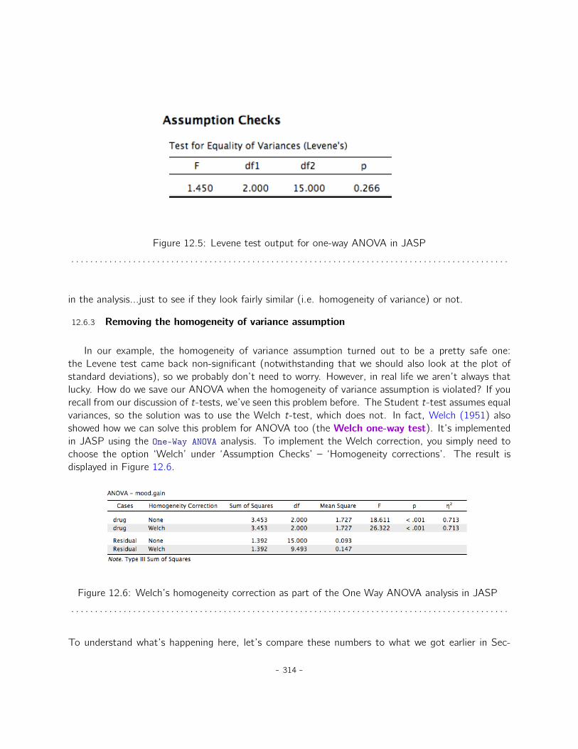
Figure 12.5: Levene test output for one-way ANOVA in JASP

. . . . . . . . . . . . . . . . . . . . . . . . . . . . . . . . . . . . . . . . . . . . . . . . . . . . . . . . . . . . . . . . . . . . . . . . . . . . . . . . . . . . . . . . . . . .

in the analysis...just to see if they look fairly similar (i.e. homogeneity of variance) or not.

12.6.3 Removing the homogeneity of variance assumption

In our example, the homogeneity of variance assumption turned out to be a pretty safe one:the Levene test came back non-significant (notwithstanding that we should also look at the plot ofstandard deviations), so we probably don’t need to worry. However, in real life we aren’t always thatlucky. How do we save our ANOVA when the homogeneity of variance assumption is violated? If yourecall from our discussion of t-tests, we’ve seen this problem before. The Student t-test assumes equalvariances, so the solution was to use the Welch t-test, which does not. In fact, Welch (1951) alsoshowed how we can solve this problem for ANOVA too (the Welch one-way test). It’s implementedin JASP using the One-Way ANOVA analysis. To implement the Welch correction, you simply need tochoose the option ‘Welch’ under ‘Assumption Checks’ – ‘Homogeneity corrections’. The result isdisplayed in Figure 12.6.

Figure 12.6: Welch’s homogeneity correction as part of the One Way ANOVA analysis in JASP

. . . . . . . . . . . . . . . . . . . . . . . . . . . . . . . . . . . . . . . . . . . . . . . . . . . . . . . . . . . . . . . . . . . . . . . . . . . . . . . . . . . . . . . . . . . .

To understand what’s happening here, let’s compare these numbers to what we got earlier in Sec-

- 314 -

tion 12.3 when we ran our original ANOVA. To save you the trouble of flicking back, this is what wegot last time: F p2, 15q “ 18.611, p ă 0.001, also shown as None under Homogeneity Correction inthe One-Way ANOVA shown in Figure 12.6.

Okay, so originally our ANOVA gave us the result F p2, 15q “ 18.6, whereas the Welch correctiongave us F p2, 9.49q “ 26.32. In other words, the Welch correction has reduced the within-groupsdegrees of freedom from 15 to 9.49, and as a result the F -value has increased from 18.6 to 26.32.

12.6.4 Checking the normality assumption

Testing the normality assumption is relatively straightforward. We covered most of what you needto know in Section 10.8. The only thing we really need to do is draw a QQ plot7. The QQ plot can beproduced in JASP by going to ‘Assumption Checks’ and checking ‘Q-Q plot of residuals’. The resultis shown in Figure 12.7 and it looks pretty normal to me.

12.7

Removing the normality assumption

Now that we’ve seen how to check for normality, we are led naturally to ask what we can do to addressviolations of normality. In the context of a one-way ANOVA, the easiest solution is probably to switchto a non-parametric test (i.e., one that doesn’t rely on any particular assumption about the kind ofdistribution involved). We’ve seen non-parametric tests before, in Chapter 10. When you only havetwo groups, the Mann-Whitney or the Wilcoxon test provides the non-parametric alternative that youneed. When you’ve got three or more groups, you can use the Kruskal-Wallis rank sum test (Kruskaland Wallis 1952). So that’s the test we’ll talk about next.

12.7.1 The logic behind the Kruskal-Wallis test

The Kruskal-Wallis test is surprisingly similar to ANOVA, in some ways. In ANOVA we started withYik , the value of the outcome variable for the ith person in the kth group. For the Kruskal-Wallis testwhat we’ll do is rank order all of these Yik values and conduct our analysis on the ranked data.

7We should also run a Shapiro-Wilk text, but that functionality is currently not available in JASP. If the Shapiro-Wilktest is not significant (i.e. p ă .05) then this indicates that the assumption of normality is not violated. However, aswith Levene’s test, if the sample size is large then a significant Shapiro-Wilk test may in fact be a false positive, wherethe assumption of normality is not violated in any substantive problematic sense for the analysis. And, similarly, a verysmall sample can produce false negatives. That’s why a visual inspection of the QQ plot is important.

- 315 -

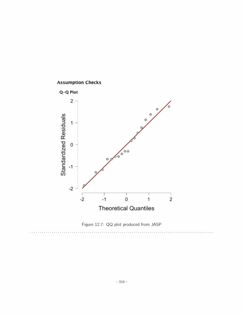
Figure 12.7: QQ plot produced from JASP

. . . . . . . . . . . . . . . . . . . . . . . . . . . . . . . . . . . . . . . . . . . . . . . . . . . . . . . . . . . . . . . . . . . . . . . . . . . . . . . . . . . . . . . . . . . .

- 316 -

So let’s let Rik refer to the ranking given to the ith member of the kth group. Now, let’s calculateRk , the average rank given to observations in the kth group

Rk “1

NK

ÿ

i

Rik

and let’s also calculate R, the grand mean rank

R “1

N

ÿ

i

ÿ

k

Rik

Now that we’ve done this, we can calculate the squared deviations from the grand mean rankR. When we do this for the individual scores, i.e., if we calculate pRik ´ Rq2, what we have is a“nonparametric” measure of how far the ik-th observation deviates from the grand mean rank. Whenwe calculate the squared deviation of the group means from the grand means, i.e., if we calculatepRk ´ Rq

2, then what we have is a nonparametric measure of how much the group deviates fromthe grand mean rank. With this in mind, we’ll follow the same logic that we did with ANOVA anddefine our ranked sums of squares measures, much like we did earlier. First, we have our “totalranked sums of squares”

RSStot “ÿ

k

ÿ

i

pRik ´ Rq2

and we can define the “between groups ranked sums of squares” like this

RSSb “ř

k

ř

ipRk ´ Rq2

“ř

k NkpRk ´ Rq2

So, if the null hypothesis is true and there are no true group differences at all, you’d expect thebetween group rank sums RSSb to be very small, much smaller than the total rank sums RSStot .Qualitatively this is very much the same as what we found when we went about constructing theANOVA F -statistic, but for technical reasons the Kruskal-Wallis test statistic, usually denoted K,is constructed in a slightly different way,

K “ pN ´ 1q ˆRSSbRSStot

and if the null hypothesis is true, then the sampling distribution of K is approximately chi-squarewith G ´ 1 degrees of freedom (where G is the number of groups). The larger the value of K, theless consistent the data are with the null hypothesis, so this is a one-sided test. We reject H0 whenK is sufficiently large.

- 317 -

12.7.2 Additional details

The description in the previous section illustrates the logic behind the Kruskal-Wallis test. At aconceptual level, this is the right way to think about how the test works. However, from a purelymathematical perspective it’s needlessly complicated. I won’t show you the derivation, but you canuse a bit of algebraic jiggery-pokerya to show that the equation for K can be rewritten as

K “12

NpN ´ 1q

ÿ

k

Nk R2k ´ 3pN ` 1q

It’s this last equation that you sometimes see given for K. This is way easier to calculate thanthe version I described in the previous section, but it’s just that it’s totally meaningless to actualhumans. It’s probably best to think of K the way I described it earlier, as an analogue of ANOVAbased on ranks. But keep in mind that the test statistic that gets calculated ends up with a ratherdifferent look to it than the one we used for our original ANOVA.

But wait, there’s more! Dear lord, why is there always more? The story I’ve told so far is onlyactually true when there are no ties in the raw data. That is, if there are no two observations thathave exactly the same value. If there are ties, then we have to introduce a correction factor tothese calculations. At this point I’m assuming that even the most diligent reader has stopped caring(or at least formed the opinion that the tie-correction factor is something that doesn’t require theirimmediate attention). So I’ll very quickly tell you how it’s calculated, and omit the tedious detailsabout why it’s done this way. Suppose we construct a frequency table for the raw data, and let fjbe the number of observations that have the j-th unique value. This might sound a bit abstract, sohere’s a concrete example from the frequency table of mood.gain from the clinicaltrials.csvdata set:

0.1 0.2 0.3 0.4 0.5 0.6 0.8 0.9 1.1 1.2 1.3 1.4 1.7 1.81 1 2 1 1 2 1 1 1 1 2 2 1 1

Looking at this table, notice that the third entry in the frequency table has a value of 2. Since thiscorresponds to a mood.gain of 0.3, this table is telling us that two people’s mood increased by 0.3.More to the point, in the mathematical notation I introduced above, this is telling us that f3 “ 2.Yay. So, now that we know this, the tie correction factor (TCF) is:

TCF “ 1´

ř

j fj3 ´ fj

N3 ´ N

The tie-corrected value of the Kruskal-Wallis statistic is obtained by dividing the value of K bythis quantity. It is this tie-corrected version that JASP calculates. And at long last, we’re actuallyfinished with the theory of the Kruskal-Wallis test. I’m sure you’re all terribly relieved that I’ve cured

- 318 -

you of the existential anxiety that naturally arises when you realise that you don’t know how tocalculate the tie-correction factor for the Kruskal-Wallis test. Right?

aA technical term.

12.7.3 How to run the Kruskal-Wallis test in JASP

Despite the horror that we’ve gone through in trying to understand what the Kruskal-Wallis testactually does, it turns out that running the test is pretty painless, since JASP has an analysis as partof the ANOVA analysis set called ‘Nonparametrics’. All you need to do is move the grouping variabledrug into the active box. What this gives us is a Kruskal-Wallis χ2 = 12.076, df = 2, p-value = 0.002,as in Figure 12.8

Figure 12.8: Kruskall-Wallis one-way non-parametric ANOVA in JASP

. . . . . . . . . . . . . . . . . . . . . . . . . . . . . . . . . . . . . . . . . . . . . . . . . . . . . . . . . . . . . . . . . . . . . . . . . . . . . . . . . . . . . . . . . . . .

12.8

Repeated measures one-way ANOVA

The one-way repeated measures ANOVA test is a statistical method of testing for significant differ-ences between three or more groups where the same participants are used in each group (or eachparticipant is closely matched with participants in other experimental groups). For this reason, thereshould always be an equal number of scores (data points) in each experimental group. This type ofdesign and analysis can also be called a ‘related ANOVA’ or a ‘within-subjects ANOVA’.

The logic behind a repeated measures ANOVA is very similar to that of an independent ANOVA(sometimes called a ‘between-subjects’ ANOVA). You’ll remember that earlier we showed that ina between-subjects ANOVA total variability is partitioned into between-groups variability (SSb) and

- 319 -

within-groups variability (SSw ), and after each is divided by the respective degrees of freedom to giveMSb and MSw (see Table 12.1) the F-ratio is calculated as:

F “MSbMSw

In a repeated measures ANOVA, the F-ratio is calculated in a similar way, but whereas in anindependent ANOVA the within-group variability (SSw ) is used as the basis for the MSw denominator,in a repeated measures ANOVA the SSw is partioned into two parts. As we are using the same subjectsin each group, we can remove the variability due to the individual differences between subjects (referredto as SSsubjects) from the within-groups variability. We won’t go into too much technical detail abouthow this is done, but essentially each subject becomes a level of a factor called subjects. The variabilityin this within-subjects factor is then calculated in the same way as any between-subjects factor. Andthen we can subtract SSsubjects from SSw to provide a smaller SSerror term:

Independent ANOVA: SSerror = SSw

Repeated Measures ANOVA: SSerror = SSw - SSsubjects

This change in SSerror term often leads to a more powerful statistical test, but this does depend onwhether the reduction in the SSerror more than compensates for the reduction in degrees of freedomfor the error term (as degrees of freedom go from (n - k)8 to (n - 1)(k - 1) (remembering that thereare more subjects in the independent ANOVA design).

12.8.1 Repeated measures ANOVA in JASP

First, we need some data. Geschwind (1972) has suggested that the exact nature of a patient’slanguage deficit following a stroke can be used to diagnose the specific region of the brain that hasbeen damaged. A researcher is concerned with identifying the specific communication difficultiesexperienced by six patients suffering from Broca’s Aphasia (a language deficit commonly experiencedfollowing a stroke).

The patients were required to complete three word recognition tasks. On the first (speech pro-duction) task, patients were required to repeat single words read out aloud by the researcher. On thesecond (conceptual) task, designed to test word comprehension, patients were required to match aseries of pictures with their correct name. On the third (syntax) task, designed to test knowledgeof correct word order, patients were asked to reorder syntactically incorrect sentences. Each patientcompleted all three tasks. The order in which patients attempted the tasks was counterbalancedbetween participants. Each task consisted of a series of 10 attempts. The number of attempts suc-cessfully completed by each patient are shown in Table 12.2. You’ll find these data in the broca.csvfile, which you can load into JASP.

8(n - k) : (number of subjects - number of groups)

- 320 -

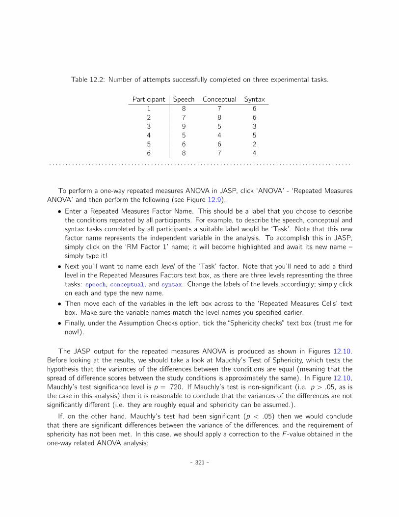
Table 12.2: Number of attempts successfully completed on three experimental tasks.

Participant Speech Conceptual Syntax1 8 7 62 7 8 63 9 5 34 5 4 55 6 6 26 8 7 4

. . . . . . . . . . . . . . . . . . . . . . . . . . . . . . . . . . . . . . . . . . . . . . . . . . . . . . . . . . . . . . . . . . . . . . . . . . . . . . . . . . . . . . . . . . . .

To perform a one-way repeated measures ANOVA in JASP, click ‘ANOVA’ - ‘Repeated MeasuresANOVA’ and then perform the following (see Figure 12.9),

• Enter a Repeated Measures Factor Name. This should be a label that you choose to describethe conditions repeated by all participants. For example, to describe the speech, conceptual andsyntax tasks completed by all participants a suitable label would be ‘Task’. Note that this newfactor name represents the independent variable in the analysis. To accomplish this in JASP,simply click on the ‘RM Factor 1’ name; it will become highlighted and await its new name –simply type it!

• Next you’ll want to name each level of the ‘Task’ factor. Note that you’ll need to add a thirdlevel in the Repeated Measures Factors text box, as there are three levels representing the threetasks: speech, conceptual, and syntax. Change the labels of the levels accordingly; simply clickon each and type the new name.

• Then move each of the variables in the left box across to the ‘Repeated Measures Cells’ textbox. Make sure the variable names match the level names you specified earlier.

• Finally, under the Assumption Checks option, tick the “Sphericity checks” text box (trust me fornow!).

The JASP output for the repeated measures ANOVA is produced as shown in Figures 12.10.Before looking at the results, we should take a look at Mauchly’s Test of Sphericity, which tests thehypothesis that the variances of the differences between the conditions are equal (meaning that thespread of difference scores between the study conditions is approximately the same). In Figure 12.10,Mauchly’s test significance level is p “ .720. If Mauchly’s test is non-significant (i.e. p ą .05, as isthe case in this analysis) then it is reasonable to conclude that the variances of the differences are notsignificantly different (i.e. they are roughly equal and sphericity can be assumed.).

If, on the other hand, Mauchly’s test had been significant (p ă .05) then we would concludethat there are significant differences between the variance of the differences, and the requirement ofsphericity has not been met. In this case, we should apply a correction to the F -value obtained in theone-way related ANOVA analysis:

- 321 -

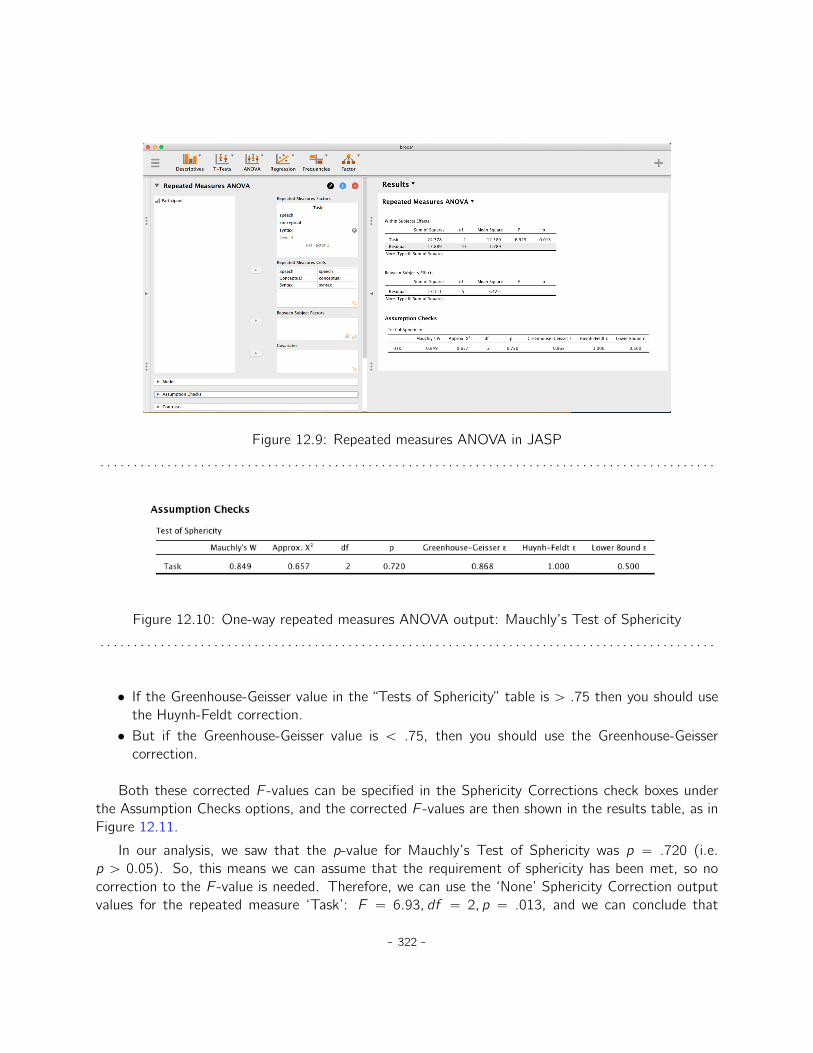
Figure 12.9: Repeated measures ANOVA in JASP

. . . . . . . . . . . . . . . . . . . . . . . . . . . . . . . . . . . . . . . . . . . . . . . . . . . . . . . . . . . . . . . . . . . . . . . . . . . . . . . . . . . . . . . . . . . .

Figure 12.10: One-way repeated measures ANOVA output: Mauchly’s Test of Sphericity

. . . . . . . . . . . . . . . . . . . . . . . . . . . . . . . . . . . . . . . . . . . . . . . . . . . . . . . . . . . . . . . . . . . . . . . . . . . . . . . . . . . . . . . . . . . .

• If the Greenhouse-Geisser value in the “Tests of Sphericity” table is ą .75 then you should usethe Huynh-Feldt correction.• But if the Greenhouse-Geisser value is ă .75, then you should use the Greenhouse-Geissercorrection.

Both these corrected F -values can be specified in the Sphericity Corrections check boxes underthe Assumption Checks options, and the corrected F -values are then shown in the results table, as inFigure 12.11.

In our analysis, we saw that the p-value for Mauchly’s Test of Sphericity was p “ .720 (i.e.p ą 0.05). So, this means we can assume that the requirement of sphericity has been met, so nocorrection to the F -value is needed. Therefore, we can use the ‘None’ Sphericity Correction outputvalues for the repeated measure ‘Task’: F “ 6.93, df “ 2, p “ .013, and we can conclude that

- 322 -

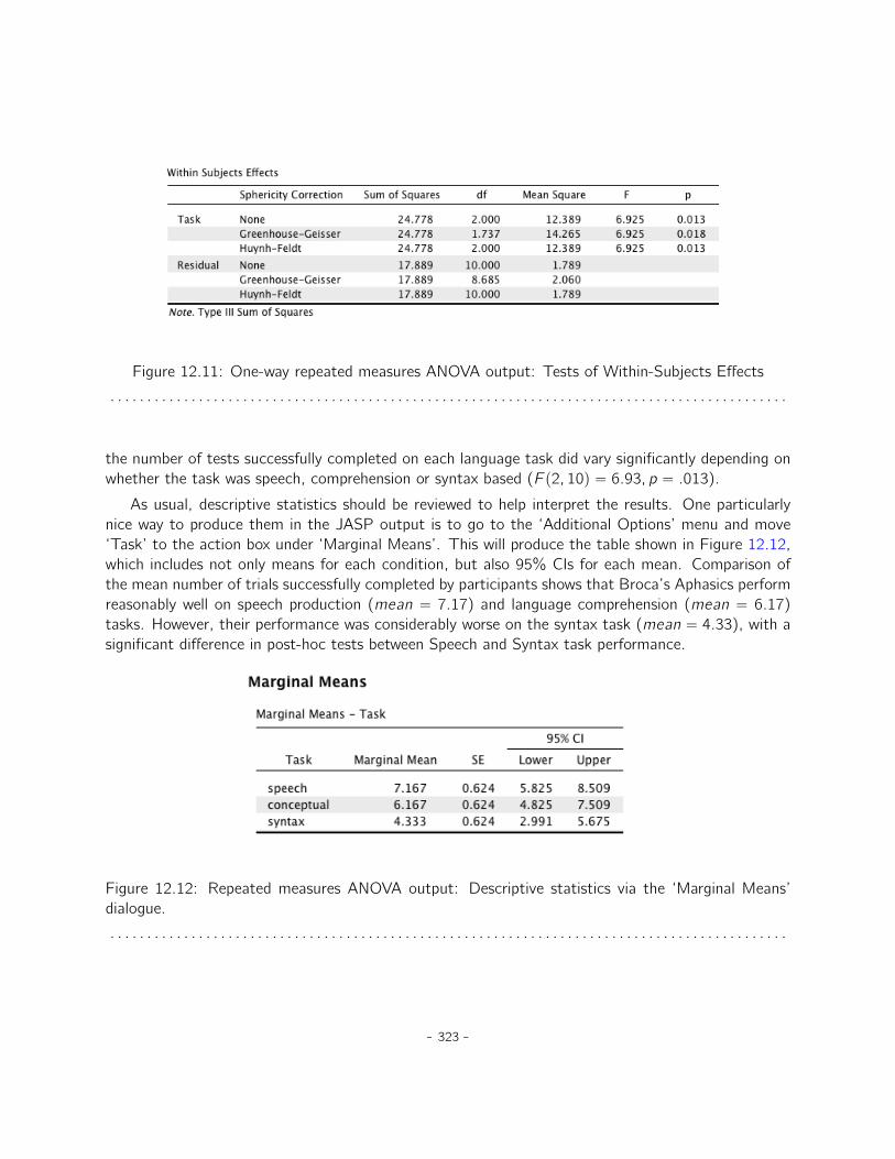
Figure 12.11: One-way repeated measures ANOVA output: Tests of Within-Subjects Effects

. . . . . . . . . . . . . . . . . . . . . . . . . . . . . . . . . . . . . . . . . . . . . . . . . . . . . . . . . . . . . . . . . . . . . . . . . . . . . . . . . . . . . . . . . . . .

the number of tests successfully completed on each language task did vary significantly depending onwhether the task was speech, comprehension or syntax based (F p2, 10q “ 6.93, p “ .013).

As usual, descriptive statistics should be reviewed to help interpret the results. One particularlynice way to produce them in the JASP output is to go to the ‘Additional Options’ menu and move‘Task’ to the action box under ‘Marginal Means’. This will produce the table shown in Figure 12.12,which includes not only means for each condition, but also 95% CIs for each mean. Comparison ofthe mean number of trials successfully completed by participants shows that Broca’s Aphasics performreasonably well on speech production (mean “ 7.17) and language comprehension (mean “ 6.17)tasks. However, their performance was considerably worse on the syntax task (mean “ 4.33), with asignificant difference in post-hoc tests between Speech and Syntax task performance.

Figure 12.12: Repeated measures ANOVA output: Descriptive statistics via the ‘Marginal Means’dialogue.

. . . . . . . . . . . . . . . . . . . . . . . . . . . . . . . . . . . . . . . . . . . . . . . . . . . . . . . . . . . . . . . . . . . . . . . . . . . . . . . . . . . . . . . . . . . .

- 323 -

12.9

The Friedman non-parametric repeated measures ANOVA test

The Friedman test is a non-parametric version of a repeated measures ANOVA and can be usedinstead of the Kruskall-Wallis test when testing for differences between three or more groups wherethe same participants are in each group, or each participant is closely matched with participants inother conditions. If the dependent variable is ordinal, or if the assumption of normality is not met,then the Friedman test can be used.

Figure 12.13: The Friedman nonparametric repeated measures ANOVA in JASP

. . . . . . . . . . . . . . . . . . . . . . . . . . . . . . . . . . . . . . . . . . . . . . . . . . . . . . . . . . . . . . . . . . . . . . . . . . . . . . . . . . . . . . . . . . . .

As with the Kruskall-Wallis test, the underlying mathematics is complicated, and won’t be pre-sented here. For the purpose of this book, it is sufficient to note that JASP calculates the tie-correctedversion of the Friedman test, and in Figure 12.13 there is an example using the Broca’s Aphasia datawe have already looked at.

It’s pretty straightforward to run a Friedman test in JASP. Just go to the ‘Nonparametrics’ menuand move ‘Task’ into the ‘RM Factor’ box. You should also click the ‘Conover’s post hoc tests’ option.

The JASP results in Figure 12.13 show a chi-square value, degrees of freedom, the p-value, and aKendall’sW value. Since the p-value is less than the level conventionally used to determine significance(p ă .05), we can conclude that there is a difference among the 3 levels of task. Conover’s posthoc tests indicate that the patients perform reasonably well on speech production (mean “ 7.2) andlanguage comprehension (mean “ 6.2) tasks. However, their performance was considerably worse onthe syntax task (median “ 4.3), with a significant difference in post-hoc tests between Speech andSyntax task performance. Do note that this significant difference only appears with the uncorrectedp-value; both the Bonferroni-corrected and Holm-corrected p-values are not significant (p “ 0.081

for both).

- 324 -

12.10

On the relationship between ANOVA and the Student t-test

There’s one last thing I want to point out before finishing. It’s something that a lot of people find kindof surprising, but it’s worth knowing about. An ANOVA with two groups is identical to the Student t-test. No, really. It’s not just that they are similar, but they are actually equivalent in every meaningfulway. I won’t try to prove that this is always true, but I will show you a single concrete demonstration.Suppose that, instead of running an ANOVA on our mood.gain ~ drug model, let’s instead do it usingtherapy as the predictor. If we run this ANOVA we get an F -statistic of F p1, 16q “ 1.71, and ap-value = 0.21. Since we only have two groups, I didn’t actually need to resort to an ANOVA, Icould have just decided to run a Student t-test. So let’s see what happens when I do that: I get at-statistic of tp16q “ ´1.3068 and a p-value = 0.21. Curiously, the p-values are identical. Once againwe obtain a value of p “ .21. But what about the test statistic? Having run a t-test instead of anANOVA, we get a somewhat different answer, namely tp16q “ ´1.3068. However, there is a fairlystraightforward relationship here. If we square the t-statistic then we get the F -statistic from before:´1.30682 “ 1.7077

12.11

Summary

There’s a fair bit covered in this chapter, but there’s still a lot missing. Most obviously, I haven’tdiscussed how to run an ANOVA when you are interested in more than one grouping variable, but thatwill be discussed in a lot of detail in Chapter 13. In terms of what we have discussed, the key topicswere:

• The basic logic behind how ANOVA works (Section 12.2) and how to run one in JASP (Sec-tion 12.3).

• How to compute an effect size for an ANOVA (Section 12.4)

• Post-hoc analysis and corrections for multiple testing (Section 12.5).

• The assumptions made by ANOVA (Section 12.6).

• How to check the homogeneity of variance assumption (Section 12.6.1) and what to do if it isviolated (Section 12.6.3).

• How to check the normality assumption (Section 12.6.4) and what to do if it is violated (Sec-tion 12.7).

• Repeated measures ANOVA (Section 12.8) and the non-parametric equivalent, the Friedmantest (Section 12.9).

- 325 -

As with all of the chapters in this book, there are quite a few different sources that I’ve reliedupon, but the one stand-out text that I’ve been most heavily influenced by is Sahai and Ageel (2000).It’s not a good book for beginners, but it’s an excellent book for more advanced readers who areinterested in understanding the mathematics behind ANOVA.

- 326 -

13. Factorial ANOVA

Over the course of the last few chapters we have done quite a lot. We have looked at statisticaltests you can use when you have one nominal predictor variable with two groups (e.g. the t-test,Chapter 10) or with three or more groups (e.g. one-way ANOVA, Chapter 12). The chapter onregression (Chapter 11) introduced a powerful new idea, that is building statistical models withmultiplecontinuous predictor variables used to explain a single outcome variable. For instance, a regressionmodel could be used to predict the number of errors a student makes in a reading comprehension testbased on the number of hours they studied for the test and their score on a standardised IQ test.

The goal in this chapter is to extend the idea of using multiple predictors into the ANOVA frame-work. For instance, suppose we were interested in using the reading comprehension test to measurestudent achievements in three different schools, and we suspect that girls and boys are developing atdifferent rates (and so would be expected to have different performance on average). Each studentis classified in two different ways: on the basis of their gender and on the basis of their school. Whatwe’d like to do is analyse the reading comprehension scores in terms of both of these grouping vari-ables. The tool for doing so is generically referred to as factorial ANOVA. However, since we havetwo grouping variables, we sometimes refer to the analysis as a two-way ANOVA, in contrast to theone-way ANOVAs that we ran in Chapter 12.

13.1

Factorial ANOVA 1: balanced designs, no interactions

When we discussed analysis of variance in Chapter 12, we assumed a fairly simple experimental design.Each person is in one of several groups and we want to know whether these groups have differentmean scores on some outcome variable. In this section, I’ll discuss a broader class of experimentaldesigns known as factorial designs, in which we have more than one grouping variable. I gave oneexample of how this kind of design might arise above. Another example appears in Chapter 12 inwhich we were looking at the effect of different drugs on the mood.gain experienced by each person.In that chapter we did find a significant effect of drug, but at the end of the chapter we also ranan analysis to see if there was an effect of therapy. We didn’t find one, but there’s something a bit

- 327 -

worrying about trying to run two separate analyses trying to predict the same outcome. Maybe thereactually is an effect of therapy on mood gain, but we couldn’t find it because it was being “hidden”by the effect of drug? In other words, we’re going to want to run a single analysis that includes bothdrug and therapy as predictors. For this analysis each person is cross-classified by the drug they weregiven (a factor with 3 levels) and what therapy they received (a factor with 2 levels). We refer to thisas a 3ˆ 2 factorial design.

If we cross-tabulate drug by therapy, using the ‘Frequencies’ - ‘Contingency Tables’ analysis inJASP (see Section 9.2), we get the table shown in Figure 13.1

Figure 13.1: JASP contingency table of drug by therapy

. . . . . . . . . . . . . . . . . . . . . . . . . . . . . . . . . . . . . . . . . . . . . . . . . . . . . . . . . . . . . . . . . . . . . . . . . . . . . . . . . . . . . . . . . . . .

As you can see, not only do we have participants corresponding to all possible combinations ofthe two factors, indicating that our design is completely crossed, it turns out that there are an equalnumber of people in each group. In other words, we have a balanced design. In this section I’lltalk about how to analyse data from balanced designs, since this is the simplest case. The story forunbalanced designs is quite tedious, so we’ll put it to one side for the moment.

13.1.1 What hypotheses are we testing?

Like one-way ANOVA, factorial ANOVA is a tool for testing certain types of hypotheses aboutpopulation means. So a sensible place to start would be to be explicit about what our hypothesesactually are. However, before we can even get to that point, it’s really useful to have some cleanand simple notation to describe the population means. Because of the fact that observations arecross-classified in terms of two different factors, there are quite a lot of different means that onemight be interested in. To see this, let’s start by thinking about all the different sample means thatwe can calculate for this kind of design. Firstly, there’s the obvious idea that we might be interestedin this list of group means:

- 328 -

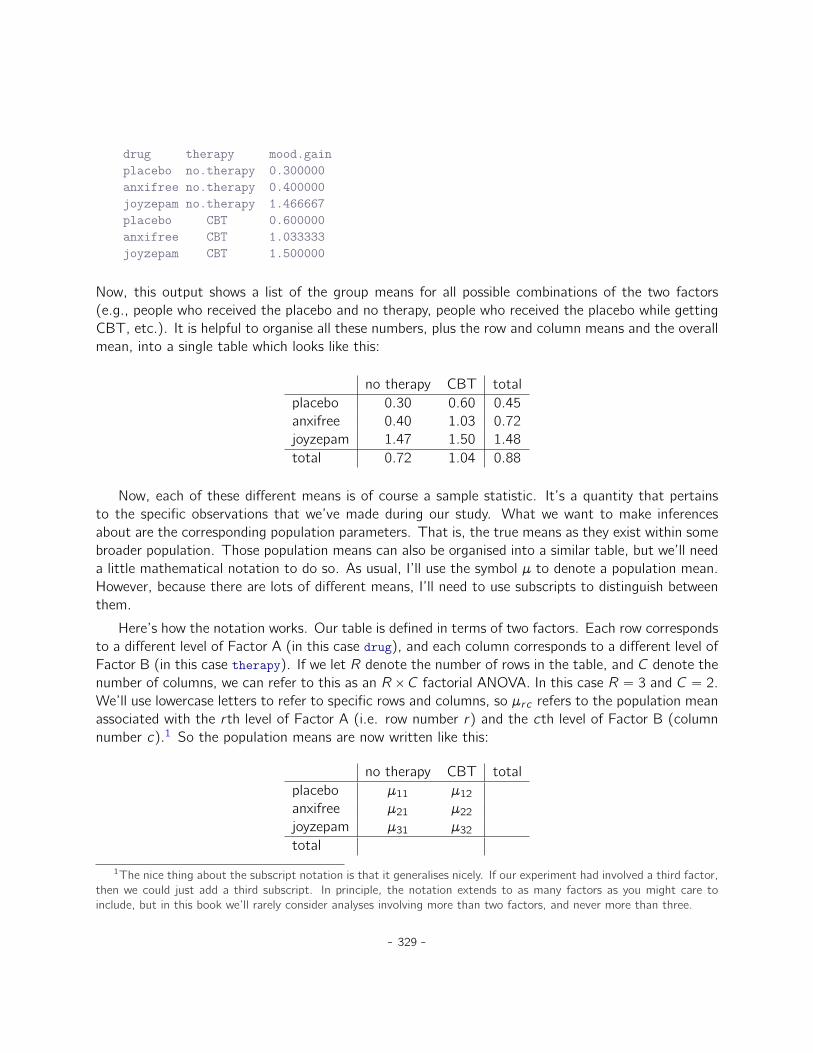
drug therapy mood.gainplacebo no.therapy 0.300000anxifree no.therapy 0.400000joyzepam no.therapy 1.466667placebo CBT 0.600000anxifree CBT 1.033333joyzepam CBT 1.500000

Now, this output shows a list of the group means for all possible combinations of the two factors(e.g., people who received the placebo and no therapy, people who received the placebo while gettingCBT, etc.). It is helpful to organise all these numbers, plus the row and column means and the overallmean, into a single table which looks like this:

no therapy CBT totalplacebo 0.30 0.60 0.45anxifree 0.40 1.03 0.72joyzepam 1.47 1.50 1.48total 0.72 1.04 0.88

Now, each of these different means is of course a sample statistic. It’s a quantity that pertainsto the specific observations that we’ve made during our study. What we want to make inferencesabout are the corresponding population parameters. That is, the true means as they exist within somebroader population. Those population means can also be organised into a similar table, but we’ll needa little mathematical notation to do so. As usual, I’ll use the symbol µ to denote a population mean.However, because there are lots of different means, I’ll need to use subscripts to distinguish betweenthem.

Here’s how the notation works. Our table is defined in terms of two factors. Each row correspondsto a different level of Factor A (in this case drug), and each column corresponds to a different level ofFactor B (in this case therapy). If we let R denote the number of rows in the table, and C denote thenumber of columns, we can refer to this as an RˆC factorial ANOVA. In this case R “ 3 and C “ 2.We’ll use lowercase letters to refer to specific rows and columns, so µrc refers to the population meanassociated with the r th level of Factor A (i.e. row number r) and the cth level of Factor B (columnnumber c).1 So the population means are now written like this:

no therapy CBT totalplacebo µ11 µ12

anxifree µ21 µ22

joyzepam µ31 µ32

total

1The nice thing about the subscript notation is that it generalises nicely. If our experiment had involved a third factor,then we could just add a third subscript. In principle, the notation extends to as many factors as you might care toinclude, but in this book we’ll rarely consider analyses involving more than two factors, and never more than three.

- 329 -

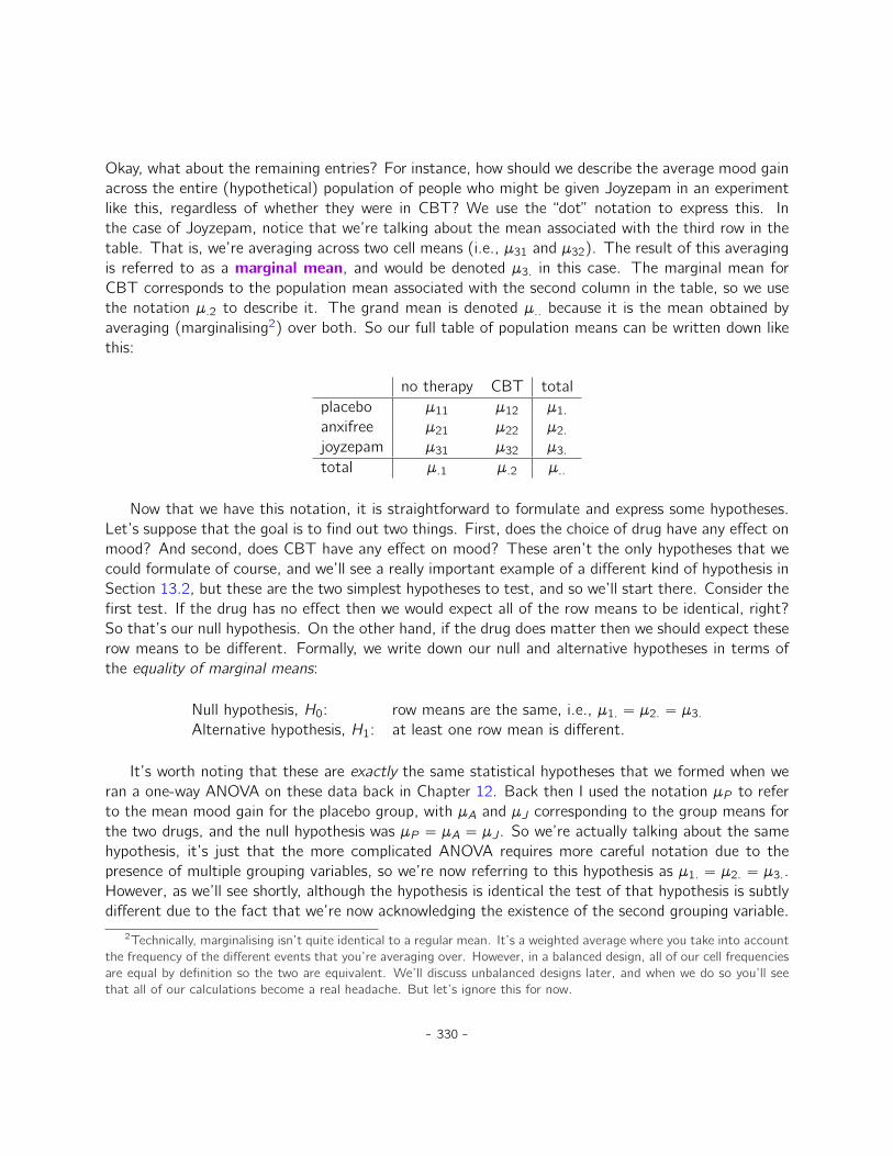
Okay, what about the remaining entries? For instance, how should we describe the average mood gainacross the entire (hypothetical) population of people who might be given Joyzepam in an experimentlike this, regardless of whether they were in CBT? We use the “dot” notation to express this. Inthe case of Joyzepam, notice that we’re talking about the mean associated with the third row in thetable. That is, we’re averaging across two cell means (i.e., µ31 and µ32). The result of this averagingis referred to as a marginal mean, and would be denoted µ3. in this case. The marginal mean forCBT corresponds to the population mean associated with the second column in the table, so we usethe notation µ.2 to describe it. The grand mean is denoted µ.. because it is the mean obtained byaveraging (marginalising2) over both. So our full table of population means can be written down likethis:

no therapy CBT totalplacebo µ11 µ12 µ1.

anxifree µ21 µ22 µ2.

joyzepam µ31 µ32 µ3.

total µ.1 µ.2 µ..

Now that we have this notation, it is straightforward to formulate and express some hypotheses.Let’s suppose that the goal is to find out two things. First, does the choice of drug have any effect onmood? And second, does CBT have any effect on mood? These aren’t the only hypotheses that wecould formulate of course, and we’ll see a really important example of a different kind of hypothesis inSection 13.2, but these are the two simplest hypotheses to test, and so we’ll start there. Consider thefirst test. If the drug has no effect then we would expect all of the row means to be identical, right?So that’s our null hypothesis. On the other hand, if the drug does matter then we should expect theserow means to be different. Formally, we write down our null and alternative hypotheses in terms ofthe equality of marginal means:

Null hypothesis, H0: row means are the same, i.e., µ1. “ µ2. “ µ3.

Alternative hypothesis, H1: at least one row mean is different.

It’s worth noting that these are exactly the same statistical hypotheses that we formed when weran a one-way ANOVA on these data back in Chapter 12. Back then I used the notation µP to referto the mean mood gain for the placebo group, with µA and µJ corresponding to the group means forthe two drugs, and the null hypothesis was µP “ µA “ µJ . So we’re actually talking about the samehypothesis, it’s just that the more complicated ANOVA requires more careful notation due to thepresence of multiple grouping variables, so we’re now referring to this hypothesis as µ1. “ µ2. “ µ3..However, as we’ll see shortly, although the hypothesis is identical the test of that hypothesis is subtlydifferent due to the fact that we’re now acknowledging the existence of the second grouping variable.

2Technically, marginalising isn’t quite identical to a regular mean. It’s a weighted average where you take into accountthe frequency of the different events that you’re averaging over. However, in a balanced design, all of our cell frequenciesare equal by definition so the two are equivalent. We’ll discuss unbalanced designs later, and when we do so you’ll seethat all of our calculations become a real headache. But let’s ignore this for now.

- 330 -

Speaking of the other grouping variable, you won’t be surprised to discover that our second hy-pothesis test is formulated the same way. However, since we’re talking about the psychological therapyrather than drugs our null hypothesis now corresponds to the equality of the column means:

Null hypothesis, H0: column means are the same, i.e., µ.1 “ µ.2Alternative hypothesis, H1: column means are different, i.e., µ.1 ‰ µ.2

13.1.2 Running the analysis in JASP

The null and alternative hypotheses that I described in the last section should seem awfully familiar.They’re basically the same as the hypotheses that we were testing in our simpler one-way ANOVAs inChapter 12. So you’re probably expecting that the hypothesis tests that are used in factorial ANOVAwill be essentially the same as the F -test from Chapter 12. You’re expecting to see references tosums of squares (SS), mean squares (MS), degrees of freedom (df), and finally an F -statistic that wecan convert into a p-value, right? Well, you’re absolutely and completely right. So much so that I’mgoing to depart from my usual approach. Throughout this book, I’ve generally taken the approachof describing the logic (and to an extent the mathematics) that underpins a particular analysis firstand only then introducing the analysis in JASP. This time I’m going to do it the other way aroundand show you how to do it in JASP first. The reason for doing this is that I want to highlight thesimilarities between the simple one-way ANOVA tool that we discussed in Chapter 12, and the morecomplicated approach that we’re going to use in this chapter.

If the data you’re trying to analyse correspond to a balanced factorial design then running youranalysis of variance is easy. To see how easy it is, let’s start by reproducing the original analysis fromChapter 12. In case you’ve forgotten, for that analysis we were using only a single factor (i.e., drug)to predict our outcome variable (i.e., mood.gain), and we got the results shown in Figure 13.2.

Figure 13.2: JASP one way ANOVA of mood.gain by drug

. . . . . . . . . . . . . . . . . . . . . . . . . . . . . . . . . . . . . . . . . . . . . . . . . . . . . . . . . . . . . . . . . . . . . . . . . . . . . . . . . . . . . . . . . . . .

Now, suppose I’m also curious to find out if therapy has a relationship to mood.gain. In lightof what we’ve seen from our discussion of multiple regression in Chapter 11, you probably won’t besurprised that all we have to do is add therapy as a second ‘Fixed Factor’ in the analysis, see Figure13.3.

- 331 -

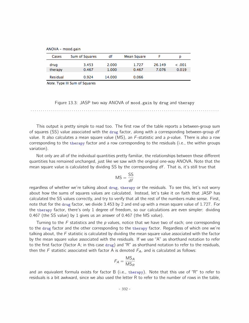
Figure 13.3: JASP two way ANOVA of mood.gain by drug and therapy

. . . . . . . . . . . . . . . . . . . . . . . . . . . . . . . . . . . . . . . . . . . . . . . . . . . . . . . . . . . . . . . . . . . . . . . . . . . . . . . . . . . . . . . . . . . .

This output is pretty simple to read too. The first row of the table reports a between-group sumof squares (SS) value associated with the drug factor, along with a corresponding between-group dfvalue. It also calculates a mean square value (MS), an F -statistic and a p-value. There is also a rowcorresponding to the therapy factor and a row corresponding to the residuals (i.e., the within groupsvariation).

Not only are all of the individual quantities pretty familiar, the relationships between these differentquantities has remained unchanged, just like we saw with the original one-way ANOVA. Note that themean square value is calculated by dividing SS by the corresponding df . That is, it’s still true that

MS “SSdf

regardless of whether we’re talking about drug, therapy or the residuals. To see this, let’s not worryabout how the sums of squares values are calculated. Instead, let’s take it on faith that JASP hascalculated the SS values correctly, and try to verify that all the rest of the numbers make sense. First,note that for the drug factor, we divide 3.453 by 2 and end up with a mean square value of 1.727. Forthe therapy factor, there’s only 1 degree of freedom, so our calculations are even simpler: dividing0.467 (the SS value) by 1 gives us an answer of 0.467 (the MS value).

Turning to the F statistics and the p values, notice that we have two of each; one correspondingto the drug factor and the other corresponding to the therapy factor. Regardless of which one we’retalking about, the F statistic is calculated by dividing the mean square value associated with the factorby the mean square value associated with the residuals. If we use “A” as shorthand notation to referto the first factor (factor A; in this case drug) and “R” as shorthand notation to refer to the residuals,then the F statistic associated with factor A is denoted FA, and is calculated as follows:

FA “MSAMSR

and an equivalent formula exists for factor B (i.e., therapy). Note that this use of “R” to refer toresiduals is a bit awkward, since we also used the letter R to refer to the number of rows in the table,

- 332 -

but I’m only going to use “R” to mean residuals in the context of SSR and MSR, so hopefully thisshouldn’t be confusing. Anyway, to apply this formula to the drugs factor we take the mean squareof 1.727 and divide it by the residual mean square value of 0.066, which gives us an F -statistic of26.149. The corresponding calculation for the therapy variable would be to divide 0.467 by 0.066

which gives 7.076 as the F -statistic. Not surprisingly, of course, these are the same values that JASPhas reported in the ANOVA table above.

Also in the ANOVA table is the calculation of the p values. Once again, there is nothing newhere. For each of our two factors what we’re trying to do is test the null hypothesis that there is norelationship between the factor and the outcome variable (I’ll be a bit more precise about this lateron). To that end, we’ve (apparently) followed a similar strategy to what we did in the one way ANOVAand have calculated an F -statistic for each of these hypotheses. To convert these to p values, all weneed to do is note that the sampling distribution for the F statistic under the null hypothesis (thatthe factor in question is irrelevant) is an F distribution. Also note that the two degrees of freedomvalues are those corresponding to the factor and those corresponding to the residuals. For the drugfactor we’re talking about an F distribution with 2 and 14 degrees of freedom (I’ll discuss degrees offreedom in more detail later). In contrast, for the therapy factor the sampling distribution is F with1 and 14 degrees of freedom.

At this point, I hope you can see that the ANOVA table for this more complicated factorialanalysis should be read in much the same way as the ANOVA table for the simpler one way analysis.In short, it’s telling us that the factorial ANOVA for our 3ˆ2 design found a significant effect of drug(F2,14 “ 26.15, p ă .001) as well as a significant effect of therapy (F1,14 “ 7.08, p “ .02). Or, to usethe more technically correct terminology, we would say that there are two main effects of drug andtherapy. At the moment, it probably seems a bit redundant to refer to these as “main” effects, but itactually does make sense. Later on, we’re going to want to talk about the possibility of “interactions”between the two factors, and so we generally make a distinction between main effects and interactioneffects.

13.1.3 How are the sum of squares calculated?

In the previous section I had two goals. Firstly, to show you that the JASP method needed to dofactorial ANOVA is pretty much the same as what we used for a one way ANOVA. The only differenceis the addition of a second factor. Secondly, I wanted to show you what the ANOVA table looks likein this case, so that you can see from the outset that the basic logic and structure behind factorialANOVA is the same as that which underpins one way ANOVA. Try to hold onto that feeling. It’sgenuinely true, insofar as factorial ANOVA is built in more or less the same way as the simpler one-wayANOVA model. It’s just that this feeling of familiarity starts to evaporate once you start digging intothe details. Traditionally, this comforting sensation is replaced by an urge to hurl abuse at the authorsof statistics textbooks.

Okay, let’s start by looking at some of those details. The explanation that I gave in the last sectionillustrates the fact that the hypothesis tests for the main effects (of drug and therapy in this case)

- 333 -

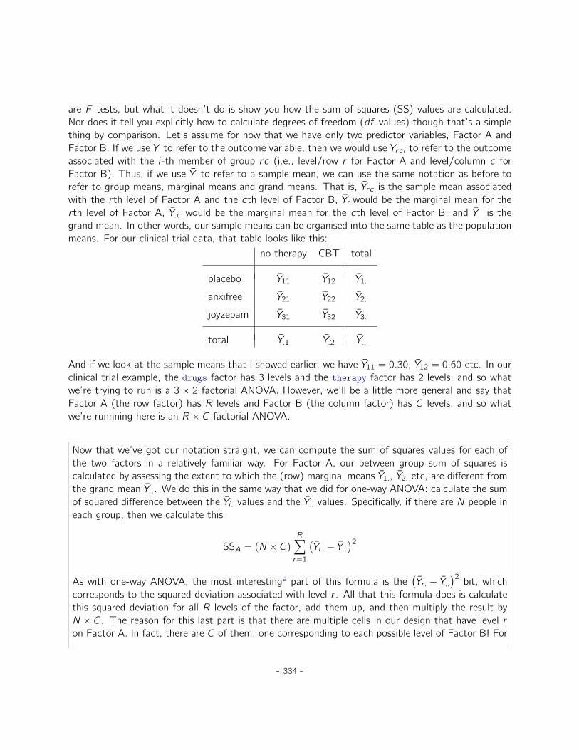
are F -tests, but what it doesn’t do is show you how the sum of squares (SS) values are calculated.Nor does it tell you explicitly how to calculate degrees of freedom (df values) though that’s a simplething by comparison. Let’s assume for now that we have only two predictor variables, Factor A andFactor B. If we use Y to refer to the outcome variable, then we would use Yrci to refer to the outcomeassociated with the i-th member of group rc (i.e., level/row r for Factor A and level/column c forFactor B). Thus, if we use Y to refer to a sample mean, we can use the same notation as before torefer to group means, marginal means and grand means. That is, Yrc is the sample mean associatedwith the r th level of Factor A and the cth level of Factor B, Yr.would be the marginal mean for ther th level of Factor A, Y.c would be the marginal mean for the cth level of Factor B, and Y.. is thegrand mean. In other words, our sample means can be organised into the same table as the populationmeans. For our clinical trial data, that table looks like this:

no therapy CBT total

placebo Y11 Y12 Y1.

anxifree Y21 Y22 Y2.

joyzepam Y31 Y32 Y3.

total Y.1 Y.2 Y..

And if we look at the sample means that I showed earlier, we have Y11 “ 0.30, Y12 “ 0.60 etc. In ourclinical trial example, the drugs factor has 3 levels and the therapy factor has 2 levels, and so whatwe’re trying to run is a 3 ˆ 2 factorial ANOVA. However, we’ll be a little more general and say thatFactor A (the row factor) has R levels and Factor B (the column factor) has C levels, and so whatwe’re runnning here is an R ˆ C factorial ANOVA.

Now that we’ve got our notation straight, we can compute the sum of squares values for each ofthe two factors in a relatively familiar way. For Factor A, our between group sum of squares iscalculated by assessing the extent to which the (row) marginal means Y1., Y2. etc, are different fromthe grand mean Y... We do this in the same way that we did for one-way ANOVA: calculate the sumof squared difference between the Yi . values and the Y.. values. Specifically, if there are N people ineach group, then we calculate this

SSA “ pN ˆ CqRÿ

r“1

`

Yr. ´ Y..˘2

As with one-way ANOVA, the most interestinga part of this formula is the`

Yr. ´ Y..˘2 bit, which

corresponds to the squared deviation associated with level r . All that this formula does is calculatethis squared deviation for all R levels of the factor, add them up, and then multiply the result byN ˆ C. The reason for this last part is that there are multiple cells in our design that have level ron Factor A. In fact, there are C of them, one corresponding to each possible level of Factor B! For

- 334 -

instance, in our example there are two different cells in the design corresponding to the anxifreedrug: one for people with no.therapy and one for the CBT group. Not only that, within each ofthese cells there are N observations. So, if we want to convert our SS value into a quantity thatcalculates the between-groups sum of squares on a “per observation” basis, we have to multiply byN ˆ C. The formula for factor B is of course the same thing, just with some subscripts shuffledaround

SSB “ pN ˆ RqCÿ

c“1

`

Y.c ´ Y..˘2

Now that we have these formulas we can check them against the JASP output from the earliersection. Once again, a dedicated spreadsheet programme is helpful for these sorts of calculations.

First, let’s calculate the sum of squares associated with the main effect of drug. There are atotal of N “ 3 people in each group and C “ 2 different types of therapy. Or, to put it anotherway, there are 3ˆ 2 “ 6 people who received any particular drug. When we do these calculations ina spreadsheet programme, we get a value of 3.45 for the sum of squares associated with the maineffect of drug. Not surprisingly, this is the same number that you get when you look up the SS valuefor the drugs factor in the ANOVA table that I presented earlier, in Figure 13.3.

We can repeat the same kind of calculation for the effect of therapy. Again there are N “ 3

people in each group, but since there are R “ 3 different drugs, this time around we note that thereare 3 ˆ 3 “ 9 people who received CBT and an additional 9 people who received the placebo. Soour calculation in this case gives us a value of 0.47 for the sum of squares associated with the maineffect of therapy. Once again, we are not surprised to see that our calculations are identical to theANOVA output in Figure 13.3.

So that’s how you calculate the SS values for the two main effects. These SS values areanalogous to the between-group sum of squares values that we calculated when doing one-wayANOVA in Chapter 12. However, it’s not a good idea to think of them as between-groups SSvalues anymore, just because we have two different grouping variables and it’s easy to get confused.In order to construct an F test, however, we also need to calculate the within-groups sum ofsquares. In keeping with the terminology that we used in the regression chapter (Chapter 11) andthe terminology that JASP uses when printing out the ANOVA table, I’ll start referring to thewithin-groups SS value as the residual sum of squares SSR.

The easiest way to think about the residual SS values in this context, I think, is to think of itas the leftover variation in the outcome variable after you take into account the differences in themarginal means (i.e., after you remove SSA and SSB). What I mean by that is we can start bycalculating the total sum of squares, which I’ll label SST . The formula for this is pretty much thesame as it was for one-way ANOVA. We take the difference between each observation Yrci and thegrand mean Y.., square the differences, and add them all up

SST “Rÿ

r“1

Cÿ

c“1

Nÿ

i“1

`

Yrci ´ Y..˘2

- 335 -

The “triple summation” here looks more complicated than it is. In the first two summations, we’resumming across all levels of Factor A (i.e., over all possible rows r in our table) and across all levelsof Factor B (i.e., all possible columns c). Each rc combination corresponds to a single group andeach group contains N people, so we have to sum across all those people (i.e., all i values) too. Inother words, all we’re doing here is summing across all observations in the data set (i.e., all possiblerci combinations).

At this point, we know the total variability of the outcome variable SST , and we know how muchof that variability can be attributed to Factor A (SSA) and how much of it can be attributed toFactor B (SSB). The residual sum of squares is thus defined to be the variability in Y that can’t beattributed to either of our two factors. In other words

SSR “ SST ´ pSSA ` SSBq

Of course, there is a formula that you can use to calculate the residual SS directly, but I think thatit makes more conceptual sense to think of it like this. The whole point of calling it a residual is thatit’s the leftover variation, and the formula above makes that clear. I should also note that, in keepingwith the terminology used in the regression chapter, it is commonplace to refer to SSA ` SSB asthe variance attributable to the “ANOVA model”, denoted SSM , and so we often say that the totalsum of squares is equal to the model sum of squares plus the residual sum of squares. Later on inthis chapter we’ll see that this isn’t just a surface similarity: ANOVA and regression are actually thesame thing under the hood.

In any case, it’s probably worth taking a moment to check that we can calculate SSR using thisformula and verify that we do obtain the same answer that JASP produces in its ANOVA table.Again, the calculations are pretty straightforward when done in a spreadsheet. We can calculate thetotal SS using the formulas above (getting an answer of total SS = 4.85) and then the residual SS( = 0.92). Yet again, we get the same answer.

aEnglish translation: “least tedious”.

13.1.4 What are our degrees of freedom?

The degrees of freedom are calculated in much the same way as for one-way ANOVA. For anygiven factor, the degrees of freedom is equal to the number of levels minus 1 (i.e., R´ 1 for the rowvariable Factor A, and C ´ 1 for the column variable Factor B). So, for the drugs factor we obtaindf “ 2, and for the therapy factor we obtain df “ 1. Later on, when we discuss the interpretationof ANOVA as a regression model (see Section 13.6), I’ll give a clearer statement of how we arriveat this number. But for the moment we can use the simple definition of degrees of freedom, namelythat the degrees of freedom equals the number of quantities that are observed, minus the number ofconstraints. So, for the drugs factor, we observe 3 separate group means, but these are constrainedby 1 grand mean, and therefore the degrees of freedom is 2. For the residuals, the logic is similar,but not quite the same. The total number of observations in our experiment is 18. The constraints

- 336 -

correspond to 1 grand mean, the 2 additional group means that the drug factor introduces, and the1 additional group mean that the the therapy factor introduces, and so our degrees of freedom is 14.As a formula, this is N ´ 1´ pR ´ 1q ´ pC ´ 1q, which simplifies to N ´ R ´ C ` 1.

13.1.5 Factorial ANOVA versus one-way ANOVAs

Now that we’ve seen how a factorial ANOVA works, it’s worth taking a moment to compare it tothe results of the one way analyses, because this will give us a really good sense of why it’s a goodidea to run the factorial ANOVA. In Chapter 12, I ran a one-way ANOVA that looked to see if thereare any differences between drugs, and a second one-way ANOVA to see if there were any differencesbetween therapies. As we saw in Section 13.1.1, the null and alternative hypotheses tested by theone-way ANOVAs are in fact identical to the hypotheses tested by the factorial ANOVA. Looking evenmore carefully at the ANOVA tables, we can see that the sum of squares associated with the factorsare identical in the two different analyses (3.45 for drug and 0.92 for therapy), as are the degrees offreedom (2 for drug, 1 for therapy). But they don’t give the same answers! Most notably, when weran the one-way ANOVA for therapy in Section 12.10 we didn’t find a significant effect (the p-valuewas .21). However, when we look at the main effect of therapy within the context of the two-wayANOVA, we do get a significant effect (p “ .019). The two analyses are clearly not the same.

Why does that happen? The answer lies in understanding how the residuals are calculated. Recallthat the whole idea behind an F -test is to compare the variability that can be attributed to a particularfactor with the variability that cannot be accounted for (the residuals). If you run a one-way ANOVAfor therapy, and therefore ignore the effect of drug, the ANOVA will end up dumping all of the drug-induced variability into the residuals! This has the effect of making the data look more noisy thanthey really are, and the effect of therapy which is correctly found to be significant in the two-wayANOVA now becomes non-significant. If we ignore something that actually matters (e.g., drug) whentrying to assess the contribution of something else (e.g., therapy) then our analysis will be distorted.Of course, it’s perfectly okay to ignore variables that are genuinely irrelevant to the phenomenon ofinterest. If we had recorded the colour of the walls, and that turned out to be a non-significantfactor in a three-way ANOVA, it would be perfectly okay to disregard it and just report the simplertwo-way ANOVA that doesn’t include this irrelevant factor. What you shouldn’t do is drop variablesthat actually make a difference!

13.1.6 What kinds of outcomes does this analysis capture?

The ANOVA model that we’ve been talking about so far covers a range of different patterns thatwe might observe in our data. For instance, in a two-way ANOVA design there are four possibilities:(a) only Factor A matters, (b) only Factor B matters, (c) both A and B matter, and (d) neither A

- 337 -

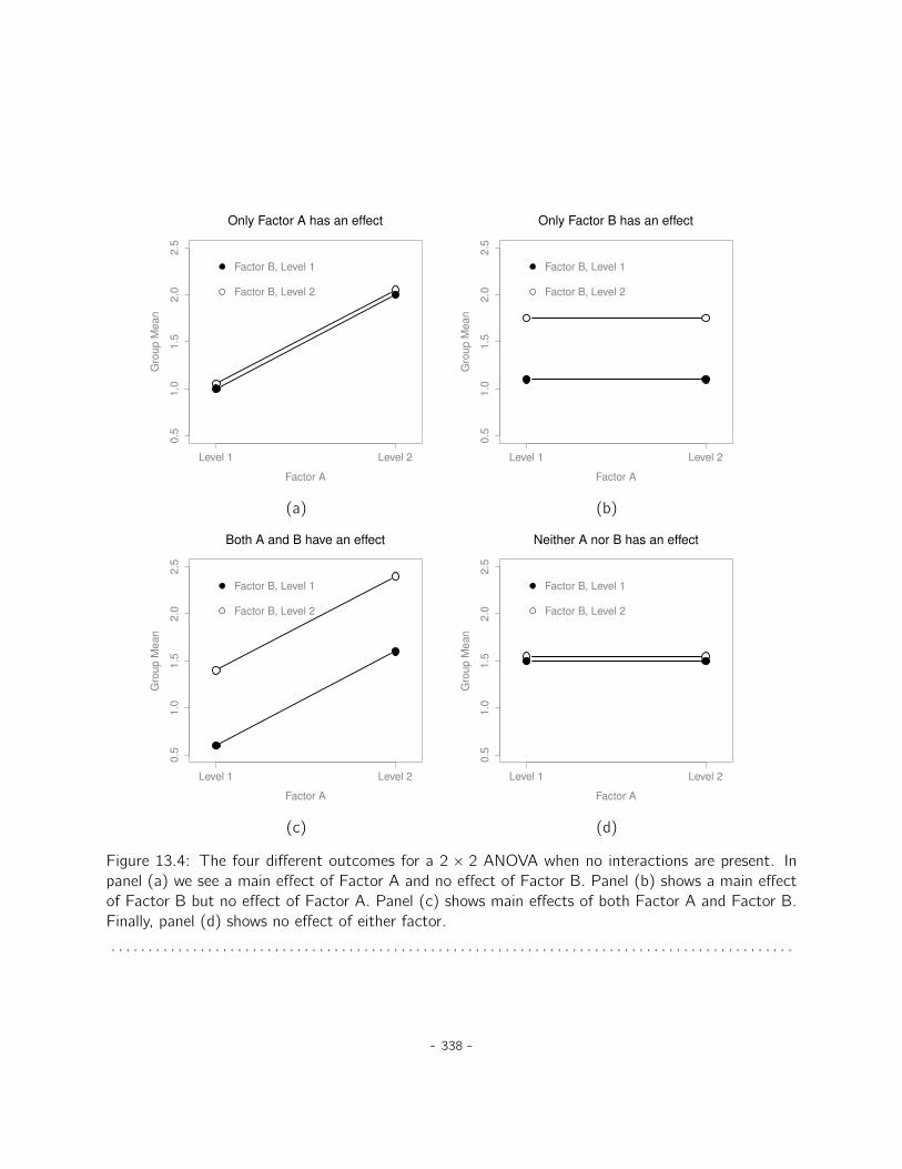
Level 1 Level 2

0.5

1.0

1.5

2.0

2.5

Only Factor A has an effect

Factor A

Gro

up

Me

an

Factor B, Level 1

Factor B, Level 2

Level 1 Level 2

0.5

1.0

1.5

2.0

2.5

Only Factor B has an effect

Factor AG

rou

p M

ea

n

Factor B, Level 1

Factor B, Level 2

(a) (b)

Level 1 Level 2

0.5

1.0

1.5

2.0

2.5

Both A and B have an effect

Factor A

Gro

up

Me

an

Factor B, Level 1

Factor B, Level 2

Level 1 Level 2

0.5

1.0

1.5

2.0

2.5

Neither A nor B has an effect

Factor A

Gro

up

Me

an

Factor B, Level 1

Factor B, Level 2

(c) (d)

Figure 13.4: The four different outcomes for a 2 ˆ 2 ANOVA when no interactions are present. Inpanel (a) we see a main effect of Factor A and no effect of Factor B. Panel (b) shows a main effectof Factor B but no effect of Factor A. Panel (c) shows main effects of both Factor A and Factor B.Finally, panel (d) shows no effect of either factor.

. . . . . . . . . . . . . . . . . . . . . . . . . . . . . . . . . . . . . . . . . . . . . . . . . . . . . . . . . . . . . . . . . . . . . . . . . . . . . . . . . . . . . . . . . . . .

- 338 -

nor B matters. An example of each of these four possibilities is plotted in Figure 13.4.

13.2

Factorial ANOVA 2: balanced designs, interactions allowed

The four patterns of data shown in Figure 13.4 are all quite realistic. There are a great many datasets that produce exactly those patterns. However, they are not the whole story and the ANOVAmodel that we have been talking about up to this point is not sufficient to fully account for a tableof group means. Why not? Well, so far we have the ability to talk about the idea that drugs caninfluence mood, and therapy can influence mood, but no way of talking about the possibility of aninteraction between the two. An interaction between A and B is said to occur whenever the effectof Factor A is different, depending on which level of Factor B we’re talking about. Several examplesof an interaction effect with the context of a 2ˆ2 ANOVA are shown in Figure 13.5. To give a moreconcrete example, suppose that the operation of Anxifree and Joyzepam is governed by quite differentphysiological mechanisms. One consequence of this is that while Joyzepam has more or less the sameeffect on mood regardless of whether one is in therapy, Anxifree is actually much more effective whenadministered in conjunction with CBT. The ANOVA that we developed in the previous section doesnot capture this idea. To get some idea of whether an interaction is actually happening here, it helpsto plot the various group means. In JASP this is done via the ANOVA ‘Descriptives Plots’ option- just move drug across into the ‘Horizontal axis’ box, and move therapy across into the ‘SeparateLines’ box. This should look something like Figure 13.6. Our main concern relates to the fact thatthe two lines aren’t parallel. The effect of CBT (difference between line with solid dots and line withopen dots) when the drug is Joyzepam (middle) appears to be near zero, even smaller than the effectof CBT when a placebo is used (right side). However, when Anxifree is administered, the effect ofCBT is larger than the placebo (left side). Is this effect real, or is this just random variation due tochance? Our original ANOVA cannot answer this question, because we make no allowances for theidea that interactions even exist! In this section, we’ll fix this problem.

13.2.1 What exactly is an interaction effect?

The key idea that we’re going to introduce in this section is that of an interaction effect. In the ANOVAmodel we have looked at so far there are only two factors involved in our model (i.e., drug and therapy).But when we add an interaction we add a new component to the model: the combination of drug andtherapy. Intuitively, the idea behind an interaction effect is fairly simple. It just means that the effectof Factor A is different, depending on which level of Factor B we’re talking about. But what does thatactually mean in terms of our data? The plot in Figure 13.5 depicts several different patterns that,although quite different to each other, would all count as an interaction effect. So it’s not entirelystraightforward to translate this qualitative idea into something mathematical that a statistician canwork with.

- 339 -

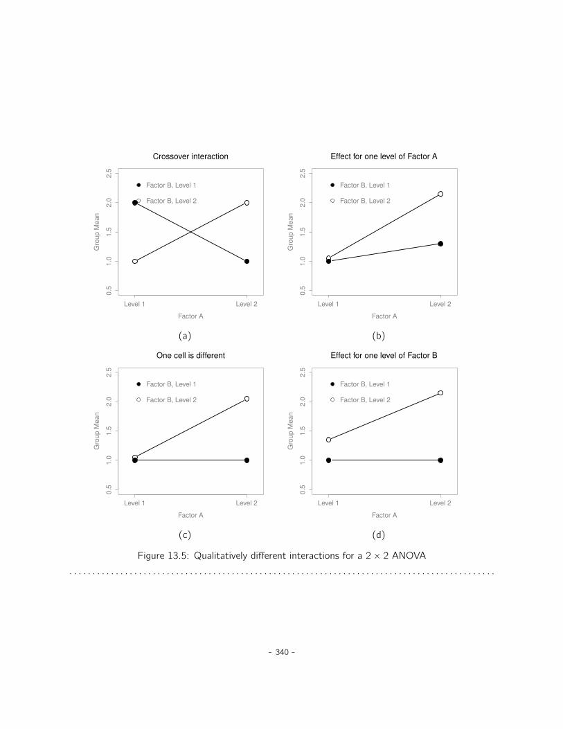
Level 1 Level 2

0.5

1.0

1.5

2.0

2.5

Crossover interaction

Factor A

Gro

up

Me

an

Factor B, Level 1

Factor B, Level 2

Level 1 Level 20

.51

.01

.52

.02

.5

Effect for one level of Factor A

Factor A

Gro

up

Me

an

Factor B, Level 1

Factor B, Level 2

(a) (b)

Level 1 Level 2

0.5

1.0

1.5

2.0

2.5

One cell is different

Factor A

Gro

up

Me

an

Factor B, Level 1

Factor B, Level 2

Level 1 Level 2

0.5

1.0

1.5

2.0

2.5

Effect for one level of Factor B

Factor A

Gro

up

Me

an

Factor B, Level 1

Factor B, Level 2

(c) (d)

Figure 13.5: Qualitatively different interactions for a 2ˆ 2 ANOVA

. . . . . . . . . . . . . . . . . . . . . . . . . . . . . . . . . . . . . . . . . . . . . . . . . . . . . . . . . . . . . . . . . . . . . . . . . . . . . . . . . . . . . . . . . . . .

- 340 -

Figure 13.6: JASP screen showing a ‘Descriptives Plot’ in ANOVA using the clinical trial data

. . . . . . . . . . . . . . . . . . . . . . . . . . . . . . . . . . . . . . . . . . . . . . . . . . . . . . . . . . . . . . . . . . . . . . . . . . . . . . . . . . . . . . . . . . . .

As a consequence, the way that the idea of an interaction effect is formalised in terms of null andalternative hypotheses is slightly difficult, and I’m guessing that a lot of readers of this book probablywon’t be all that interested. Even so, I’ll try to give the basic idea here.

To start with, we need to be a little more explicit about our main effects. Consider the maineffect of Factor A (drug in our running example). We originally formulated this in terms of the nullhypothesis that the two marginal means µr. are all equal to each other. Obviously, if all of these areequal to each other, then they must also be equal to the grand mean µ.. as well, right? So what wecan do is define the effect of Factor A at level r to be equal to the difference between the marginalmean µr. and the grand mean µ... Let’s denote this effect by αr , and note that

αr “ µr. ´ µ..

Now, by definition all of the αr values must sum to zero, for the same reason that the average ofthe marginal means µr. must be the grand mean µ... We can similarly define the effect of Factor Bat level i to be the difference between the column marginal mean µ.c and the grand mean µ..

βc “ µ.c ´ µ..

- 341 -

and once again, these βc values must sum to zero. The reason that statisticians sometimes like totalk about the main effects in terms of these αr and βc values is that it allows them to be preciseabout what it means to say that there is no interaction effect. If there is no interaction at all, thenthese αr and βc values will perfectly describe the group means µrc . Specifically, it means that

µrc “ µ.. ` αr ` βc

That is, there’s nothing special about the group means that you couldn’t predict perfectly by knowingall the marginal means. And that’s our null hypothesis, right there. The alternative hypothesis isthat

µrc ‰ µ.. ` αr ` βc

for at least one group rc in our table. However, statisticians often like to write this slightly differently.They’ll usually define the specific interaction associated with group rc to be some number, awkwardlyreferred to as pαβqrc , and then they will say that the alternative hypothesis is that

µrc “ µ.. ` αr ` βc ` pαβqrc

where pαβqrc is non-zero for at least one group. This notation is kind of ugly to look at, but it ishandy as we’ll see in the next section when discussing how to calculate the sum of squares.

13.2.2 Calculating sums of squares for the interaction

How should we calculate the sum of squares for the interaction terms, SSA:B? Well, first off,it helps to notice how the previous section defined the interaction effect in terms of the extent towhich the actual group means differ from what you’d expect by just looking at the marginal means.Of course, all of those formulas refer to population parameters rather than sample statistics, so wedon’t actually know what they are. However, we can estimate them by using sample means in placeof population means. So for Factor A, a good way to estimate the main effect at level r is as thedifference between the sample marginal mean Yrc and the sample grand mean Y... That is, we woulduse this as our estimate of the effect

αr “ Yr. ´ Y..

Similarly, our estimate of the main effect of Factor B at level c can be defined as follows

βc “ Y.c ´ Y..

Now, if you go back to the formulas that I used to describe the SS values for the two main effects,you’ll notice that these effect terms are exactly the quantities that we were squaring and summing!So, what’s the analog of this for interaction terms? The answer to this can be found by firstrearranging the formula for the group means µrc under the alternative hypothesis, so that we get

- 342 -

this

pαβqrc “ µrc ´ µ.. ´ αr ´ βc

“ µrc ´ µ.. ´ pµr. ´ µ..q ´ pµ.c ´ µ..q

“ µrc ´ µr. ´ µ.c ` µ..

So, once again if we substitute our sample statistics in place of the population means, we get thefollowing as our estimate of the interaction effect for group rc , which is

ˆpαβqrc “ Yrc ´ Yr. ´ Y.c ` Y..

Now all we have to do is sum all of these estimates across all R levels of Factor A and all C levels ofFactor B, and we obtain the following formula for the sum of squares associated with the interactionas a whole

SSA:B “ NRÿ

r“1

Cÿ

c“1

`

Yrc ´ Yr. ´ Y.c ` Y..˘2

where we multiply by N because there are N observations in each of the groups, and we want our SSvalues to reflect the variation among observations accounted for by the interaction, not the variationamong groups.

Now that we have a formula for calculating SSA:B, it’s important to recognise that the interactionterm is part of the model (of course), so the total sum of squares associated with the model, SSM ,is now equal to the sum of the three relevant SS values, SSA ` SSB ` SSA:B. The residual sum ofsquares SSR is still defined as the leftover variation, namely SST ´ SSM , but now that we have theinteraction term this becomes

SSR “ SST ´ pSSA ` SSB ` SSA:Bq

As a consequence, the residual sum of squares SSR will be smaller than in our original ANOVA thatdidn’t include interactions.

13.2.3 Degrees of freedom for the interaction

Calculating the degrees of freedom for the interaction is, once again, slightly trickier than thecorresponding calculation for the main effects. To start with, let’s think about the ANOVA model asa whole. Once we include interaction effects in the model we’re allowing every single group to havea unique mean, µrc . For an R ˆ C factorial ANOVA, this means that there are R ˆ C quantities ofinterest in the model and only the one constraint: all of the group means need to average out to thegrand mean. So the model as a whole needs to have pR ˆ Cq ´ 1 degrees of freedom. But the maineffect of Factor A has R ´ 1 degrees of freedom, and the main effect of Factor B has C ´ 1 degrees

- 343 -

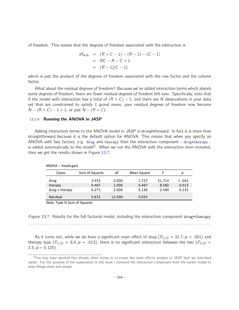
of freedom. This means that the degrees of freedom associated with the interaction is

dfA:B “ pR ˆ C ´ 1q ´ pR ´ 1q ´ pC ´ 1q

“ RC ´ R ´ C ` 1

“ pR ´ 1qpC ´ 1q

which is just the product of the degrees of freedom associated with the row factor and the columnfactor.

What about the residual degrees of freedom? Because we’ve added interaction terms which absorbsome degrees of freedom, there are fewer residual degrees of freedom left over. Specifically, note thatif the model with interaction has a total of pR ˆ Cq ´ 1, and there are N observations in your dataset that are constrained to satisfy 1 grand mean, your residual degrees of freedom now becomeN ´ pR ˆ Cq ´ 1` 1, or just N ´ pR ˆ Cq.

13.2.4 Running the ANOVA in JASP

Adding interaction terms to the ANOVA model in JASP is straightforward. In fact it is more thanstraightforward because it is the default option for ANOVA. This means that when you specify anANOVA with two factors, e.g. drug and therapy then the interaction component - drug*therapy -is added automatically to the model3. When we run the ANOVA with the interaction term included,then we get the results shown in Figure 13.7.

Figure 13.7: Results for the full factorial model, including the interaction component drug*therapy

. . . . . . . . . . . . . . . . . . . . . . . . . . . . . . . . . . . . . . . . . . . . . . . . . . . . . . . . . . . . . . . . . . . . . . . . . . . . . . . . . . . . . . . . . . . .

As it turns out, while we do have a significant main effect of drug (F2,12 “ 31.7, p ă .001) andtherapy type (F1,12 “ 8.6, p “ .013), there is no significant interaction between the two (F2,12 “

2.5, p “ 0.125).

3You may have spotted this already when trying to re-create the main effects analysis in JASP that we describedearlier. For the purpose of the explanation in this book I removed the interaction component from the earlier model tokeep things clean and simple

- 344 -

13.2.5 Interpreting the results

There’s a couple of very important things to consider when interpreting the results of factorialANOVA. First, there’s the same issue that we had with one-way ANOVA, which is that if you obtaina significant main effect of (say) drug, it doesn’t tell you anything about which drugs are different toone another. To find that out, you need to run additional analyses. We’ll talk about some analysesthat you can run in Sections 13.7 and 13.8. The same is true for interaction effects. Knowing thatthere’s a significant interaction doesn’t tell you anything about what kind of interaction exists. Again,you’ll need to run additional analyses.

Secondly, there’s a very peculiar interpretation issue that arises when you obtain a significantinteraction effect but no corresponding main effect. This happens sometimes. For instance, in thecrossover interaction shown in Figure 13.5a, this is exactly what you’d find. In this case, neither ofthe main effects would be significant, but the interaction effect would be. This is a difficult situationto interpret, and people often get a bit confused about it. The general advice that statisticians like togive in this situation is that you shouldn’t pay much attention to the main effects when an interactionis present. The reason they say this is that, although the tests of the main effects are perfectly validfrom a mathematical point of view, when there is a significant interaction effect the main effects rarelytest interesting hypotheses. Recall from Section 13.1.1 that the null hypothesis for a main effect isthat the marginal means are equal to each other, and that a marginal mean is formed by averagingacross several different groups. But if you have a significant interaction effect then you know thatthe groups that comprise the marginal mean aren’t homogeneous, so it’s not really obvious why youwould even care about those marginal means.

Here’s what I mean. Again, let’s stick with a clinical example. Suppose that we had a 2ˆ2 designcomparing two different treatments for phobias (e.g., systematic desensitisation vs flooding), and twodifferent anxiety reducing drugs (e.g., Anxifree vs Joyzepam). Now, suppose what we found was thatAnxifree had no effect when desensitisation was the treatment, and Joyzepam had no effect whenflooding was the treatment. But both were pretty effective for the other treatment. This is a classiccrossover interaction, and what we’d find when running the ANOVA is that there is no main effectof drug, but a significant interaction. Now, what does it actually mean to say that there’s no maineffect? Well, it means that if we average over the two different psychological treatments, then theaverage effect of Anxifree and Joyzepam is the same. But why would anyone care about that? Whentreating someone for phobias it is never the case that a person can be treated using an “average”of flooding and desensitisation. That doesn’t make a lot of sense. You either get one or the other.For one treatment one drug is effective, and for the other treatment the other drug is effective. Theinteraction is the important thing and the main effect is kind of irrelevant.

This sort of thing happens a lot. The main effect are tests of marginal means, and when aninteraction is present we often find ourselves not being terribly interested in marginal means becausethey imply averaging over things that the interaction tells us shouldn’t be averaged! Of course, it’snot always the case that a main effect is meaningless when an interaction is present. Often you canget a big main effect and a very small interaction, in which case you can still say things like “drug Ais generally more effective than drug B” (because there was a big effect of drug), but you’d need to

- 345 -

modify it a bit by adding that “the difference in effectiveness was different for different psychologicaltreatments”. In any case, the main point here is that whenever you get a significant interaction youshould stop and think about what the main effect actually means in this context. Don’t automaticallyassume that the main effect is interesting.

13.3

Effect size

The effect size calculation for a factorial ANOVA is pretty similar to those used in one way ANOVA(see Section 12.4). Specifically, we can use η2 (eta-squared) as a simple way to measure how bigthe overall effect is for any particular term. As before, η2 is defined by dividing the sum of squaresassociated with that term by the total sum of squares. For instance, to determine the size of the maineffect of Factor A, we would use the following formula:

η2A “

SSASST

As before, this can be interpreted in much the same way as R2 in regression.4 It tells you the proportionof variance in the outcome variable that can be accounted for by the main effect of Factor A. It istherefore a number that ranges from 0 (no effect at all) to 1 (accounts for all of the variability in theoutcome). Moreover, the sum of all the η2 values, taken across all the terms in the model, will sumto the the total R2 for the ANOVA model. If, for instance, the ANOVA model fits perfectly (i.e.,there is no within-groups variability at all!), the η2 values will sum to 1. Of course, that rarely if everhappens in real life.

However, when doing a factorial ANOVA, there is a second measure of effect size that people liketo report, known as partial η2. The idea behind partial η2 (which is sometimes denoted pη2 or η2

p) isthat, when measuring the effect size for a particular term (say, the main effect of Factor A), you wantto deliberately ignore the other effects in the model (e.g., the main effect of Factor B). That is, youwould pretend that the effect of all these other terms is zero, and then calculate what the η2 valuewould have been. This is actually pretty easy to calculate. All you have to do is remove the sum ofsquares associated with the other terms from the denominator. In other words, if you want the partialη2 for the main effect of Factor A, the denominator is just the sum of the SS values for Factor A andthe residuals

partial η2A “

SSASSA ` SSR

This will always give you a larger number than η2, which the cynic in me suspects accounts for thepopularity of partial η2. And once again you get a number between 0 and 1, where 0 represents noeffect. However, it’s slightly trickier to interpret what a large partial η2 value means. In particular,

4This chapter seems to be setting a new record for the number of different things that the letter R can stand for. Sofar we have R referring to the software package, the number of rows in our table of means, the residuals in the model,and now the correlation coefficient in a regression. Sorry. We clearly don’t have enough letters in the alphabet. However,I’ve tried pretty hard to be clear on which thing R is referring to in each case.

- 346 -

you can’t actually compare the partial η2 values across terms! Suppose, for instance, there is nowithin-groups variability at all: if so, SSR “ 0. What that means is that every term has a partialη2 value of 1. But that doesn’t mean that all terms in your model are equally important, or indeedthat they are equally large. All it mean is that all terms in your model have effect sizes that are largerelative to the residual variation. It is not comparable across terms.

To see what I mean by this, it’s useful to see a concrete example. First, let’s have a look at theeffect sizes for the original ANOVA without the interaction term, from Figure 13.3:

eta.sq partial.eta.sqdrug 0.71 0.79therapy 0.10 0.34

Looking at the η2 values first, we see that drug accounts for 71% of the variance (i.e. η2 “ 0.71)in mood.gain, whereas therapy only accounts for 10%. This leaves a total of 19% of the variationunaccounted for (i.e., the residuals constitute 19% of the variation in the outcome). Overall, thisimplies that we have a very large effect5 of drug and a modest effect of therapy.

Now let’s look at the partial η2 values, shown in Figure 13.3. Because the effect of therapy isn’tall that large, controlling for it doesn’t make much of a difference, so the partial η2 for drug doesn’tincrease very much, and we obtain a value of pη2 “ 0.79). In contrast, because the effect of drug wasvery large, controlling for it makes a big difference, and so when we calculate the partial η2 for therapyyou can see that it rises to pη2 “ 0.34. The question that we have to ask ourselves is, what do thesepartial η2 values actually mean? The way I generally interpret the partial η2 for the main effect ofFactor A is to interpret it as a statement about a hypothetical experiment in which only Factor A wasbeing varied. So, even though in this experiment we varied both A and B, we can easily imagine anexperiment in which only Factor A was varied, and the partial η2 statistic tells you how much of thevariance in the outcome variable you would expect to see accounted for in that experiment. However,it should be noted that this interpretation, like many things associated with main effects, doesn’t makea lot of sense when there is a large and significant interaction effect.

Speaking of interaction effects, here’s what we get when we calculate the effect sizes for the modelthat includes the interaction term, as in Figure 13.7. To get these in JASP, simply select ‘AdditionalOptions’ - ‘Estimates of effect size’, and choose the measures you want. As you can see, the η2

values for the main effects don’t change, but the partial η2 values do:

eta.sq partial.eta.sqdrug 0.71 0.84therapy 0.10 0.42drug*therapy 0.06 0.29

5Implausibly large, I would think. The artificiality of this data set is really starting to show!

- 347 -

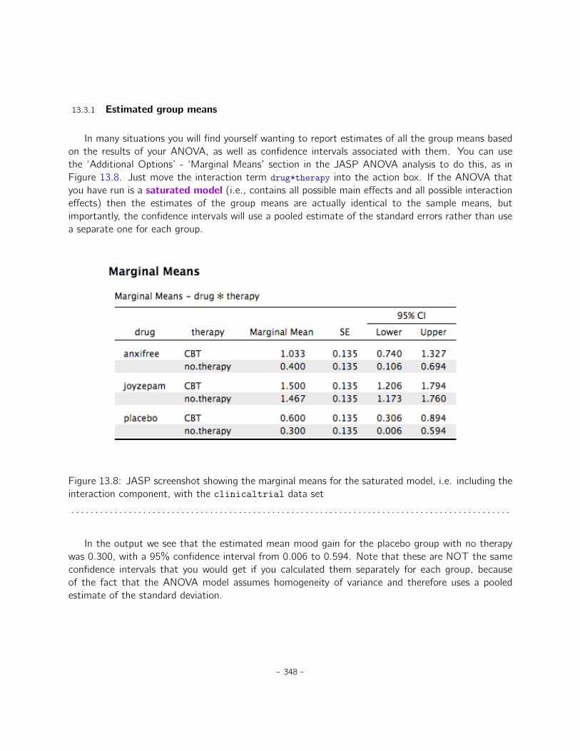
13.3.1 Estimated group means

In many situations you will find yourself wanting to report estimates of all the group means basedon the results of your ANOVA, as well as confidence intervals associated with them. You can usethe ‘Additional Options’ - ‘Marginal Means’ section in the JASP ANOVA analysis to do this, as inFigure 13.8. Just move the interaction term drug*therapy into the action box. If the ANOVA thatyou have run is a saturated model (i.e., contains all possible main effects and all possible interactioneffects) then the estimates of the group means are actually identical to the sample means, butimportantly, the confidence intervals will use a pooled estimate of the standard errors rather than usea separate one for each group.

Figure 13.8: JASP screenshot showing the marginal means for the saturated model, i.e. including theinteraction component, with the clinicaltrial data set

. . . . . . . . . . . . . . . . . . . . . . . . . . . . . . . . . . . . . . . . . . . . . . . . . . . . . . . . . . . . . . . . . . . . . . . . . . . . . . . . . . . . . . . . . . . .

In the output we see that the estimated mean mood gain for the placebo group with no therapywas 0.300, with a 95% confidence interval from 0.006 to 0.594. Note that these are NOT the sameconfidence intervals that you would get if you calculated them separately for each group, becauseof the fact that the ANOVA model assumes homogeneity of variance and therefore uses a pooledestimate of the standard deviation.

- 348 -

13.4

Assumption checking

As with one-way ANOVA, the key assumptions of factorial ANOVA are homogeneity of variance(all groups have the same standard deviation), normality of the residuals, and independence of theobservations. The first two are things we can check for. The third is something that you needto assess yourself by asking if there are any special relationships between different observations, forexample repeated measures where the independent variable is time so there is a relationship betweenthe observations at time one and time two: observations at different time points are from the samepeople. Additionally, if you aren’t using a saturated model (e.g., if you’ve omitted the interactionterms) then you’re also assuming that the omitted terms aren’t important. Of course, you can checkthis last one by running an ANOVA with the omitted terms included and see if they’re significant, sothat’s pretty easy. What about homogeneity of variance and normality of the residuals? As it turnsout, these are pretty easy to check. It’s no different to the checks we did for a one-way ANOVA.

13.4.1 Homogeneity of variance

As mentioned in Section 12.6.1 it’s a good idea to visually inspect a plot of the standard deviationscompared across different groups / categories, and also see if the Levene test is consistent with thevisual inspection. The theory behind the Levene test was discussed in Section 12.6.1, so I won’tdiscuss it again. This test expects that you have a saturated model (i.e., including all of the relevantterms), because the test is primarily concerned with the within-group variance, and it doesn’t reallymake a lot of sense to calculate this any way other than with respect to the full model. The Levenetest can be specified under the ANOVA ‘Assumption Checks’ - ‘Homogeneity tests’ option in JASP,with the result shown as in Figure 13.9. The fact that the Levene test is non-significant means that,providing it is consistent with a visual inspection of the plot of standard deviations, we can safelyassume that the homogeneity of variance assumption is not violated.

13.4.2 Normality of residuals

As with one-way ANOVA we can test for the normality of residuals in a straightforward fashion (seeSection 12.6.4). Primarily though, it’s generally a good idea to examine the residuals graphically usinga QQ plot. See Figure 13.9.

- 349 -

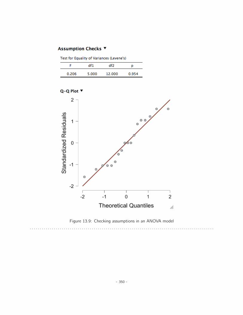
Figure 13.9: Checking assumptions in an ANOVA model

. . . . . . . . . . . . . . . . . . . . . . . . . . . . . . . . . . . . . . . . . . . . . . . . . . . . . . . . . . . . . . . . . . . . . . . . . . . . . . . . . . . . . . . . . . . .

- 350 -

13.5

Analysis of Covariance (ANCOVA)

A variation in ANOVA is when you have an additional continuous variable that you think might berelated to the dependent variable. This additional variable can be added to the analysis as a covariate,in the aptly named analysis of covariance (ANCOVA).

In ANCOVA the values of the dependent variable are “adjusted” for the influence of the covariate,and then the “adjusted” score means are tested between groups in the usual way. This technique canincrease the precision of an experiment, and therefore provide a more “powerful” test of the equalityof group means in the dependent variable. How does ANCOVA do this? Well, although the covariateitself is typically not of any experimental interest, adjustment for the covariate can decrease theestimate of experimental error and thus, by reducing error variance, precision is increased. This meansthat an inappropriate failure to reject the null hypothesis (false negative or type II error) is less likely.

Despite this advantage, ANCOVA runs the risk of undoing real differences between groups, andthis should be avoided. Look at Figure 13.10, for example, which shows a plot of Statistics anxietyagainst age and shows two distinct groups – students who have either an Arts or Science backgroundor preference. ANCOVA with age as a covariate might lead to the conclusion that statistics anxietydoes not differ in the two groups. Would this conclusion be reasonable – probably not because theages of the two groups do not overlap and analysis of variance has essentially “extrapolated into aregion with no data” (Everitt 1996, p. 68).

Clearly, careful thought needs to be given to an analysis of covariance with distinct groups. Thisapplies to both one-way and factorial designs, as ANCOVA can be used with both.

13.5.1 Running ANCOVA in JASP

A health psychologist was interested in the effect of routine cycling and stress on happiness levels,with age as a covariate. You can find the dataset in the file ancova.csv. Open this file in JASP andthen, to undertake an ANCOVA, select ‘ANOVA’ - ‘ANCOVA’ to open the ANCOVA analysis window(Figure 13.11). Highlight the dependent variable ‘happiness’ and transfer it into the ‘DependentVariable’ text box. Highlight the independent variables ‘stress’ and ‘commute’ and transfer theminto the ‘Fixed Factors’ text box. Highlight the covariate ‘age’ and transfer it into the ‘Covariates’text box. Then click on ‘Additional Options’ - ‘Marginal Means’ and transfer the interaction termstress*commute into the action box.

An ANCOVA table is produced in the JASP results window (Figure 13.11). The F value forthe covariate ‘age’ is significant at p “ .023, suggesting that age is an important predictor of thedependent variable happiness. When we look at the estimated marginal mean scores, adjustmentshave been made (compared to an analysis without the covariate) because of the inclusion of thecovariate ‘age’ in this ANCOVA. A plot (Figure 13.12) is a good way of visualising and interpreting

- 351 -

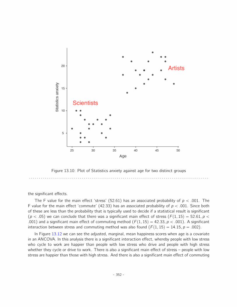
Figure 13.10: Plot of Statistics anxiety against age for two distinct groups

. . . . . . . . . . . . . . . . . . . . . . . . . . . . . . . . . . . . . . . . . . . . . . . . . . . . . . . . . . . . . . . . . . . . . . . . . . . . . . . . . . . . . . . . . . . .

the significant effects.

The F value for the main effect ‘stress’ (52.61) has an associated probability of p ă .001. TheF value for the main effect ‘commute’ (42.33) has an associated probability of p ă .001. Since bothof these are less than the probability that is typically used to decide if a statistical result is significant(p ă .05) we can conclude that there was a significant main effect of stress (F p1, 15q “ 52.61, p ă

.001) and a significant main effect of commuting method (F p1, 15q “ 42.33, p ă .001). A significantinteraction between stress and commuting method was also found (F p1, 15q “ 14.15, p “ .002).

In Figure 13.12 we can see the adjusted, marginal, mean happiness scores when age is a covariatein an ANCOVA. In this analysis there is a significant interaction effect, whereby people with low stresswho cycle to work are happier than people with low stress who drive and people with high stresswhether they cycle or drive to work. There is also a significant main effect of stress – people with lowstress are happier than those with high stress. And there is also a significant main effect of commuting

- 352 -

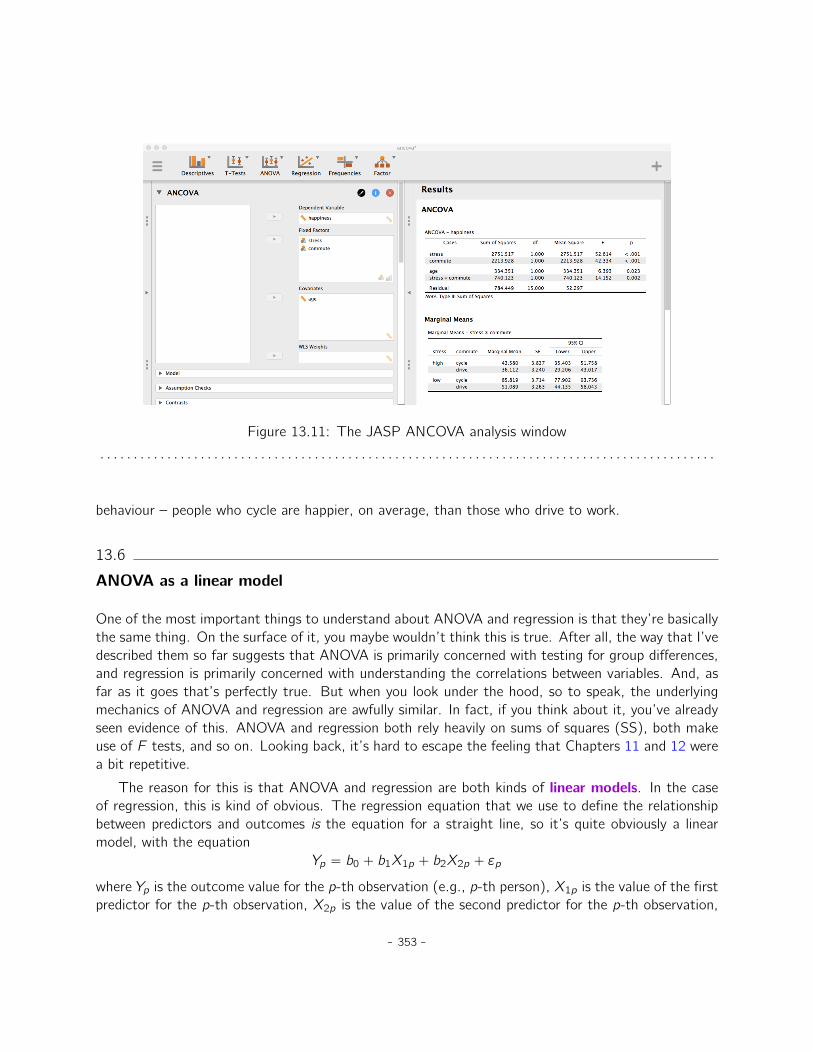
Figure 13.11: The JASP ANCOVA analysis window

. . . . . . . . . . . . . . . . . . . . . . . . . . . . . . . . . . . . . . . . . . . . . . . . . . . . . . . . . . . . . . . . . . . . . . . . . . . . . . . . . . . . . . . . . . . .

behaviour – people who cycle are happier, on average, than those who drive to work.

13.6

ANOVA as a linear model

One of the most important things to understand about ANOVA and regression is that they’re basicallythe same thing. On the surface of it, you maybe wouldn’t think this is true. After all, the way that I’vedescribed them so far suggests that ANOVA is primarily concerned with testing for group differences,and regression is primarily concerned with understanding the correlations between variables. And, asfar as it goes that’s perfectly true. But when you look under the hood, so to speak, the underlyingmechanics of ANOVA and regression are awfully similar. In fact, if you think about it, you’ve alreadyseen evidence of this. ANOVA and regression both rely heavily on sums of squares (SS), both makeuse of F tests, and so on. Looking back, it’s hard to escape the feeling that Chapters 11 and 12 werea bit repetitive.

The reason for this is that ANOVA and regression are both kinds of linear models. In the caseof regression, this is kind of obvious. The regression equation that we use to define the relationshipbetween predictors and outcomes is the equation for a straight line, so it’s quite obviously a linearmodel, with the equation

Yp “ b0 ` b1X1p ` b2X2p ` εp

where Yp is the outcome value for the p-th observation (e.g., p-th person), X1p is the value of the firstpredictor for the p-th observation, X2p is the value of the second predictor for the p-th observation,

- 353 -

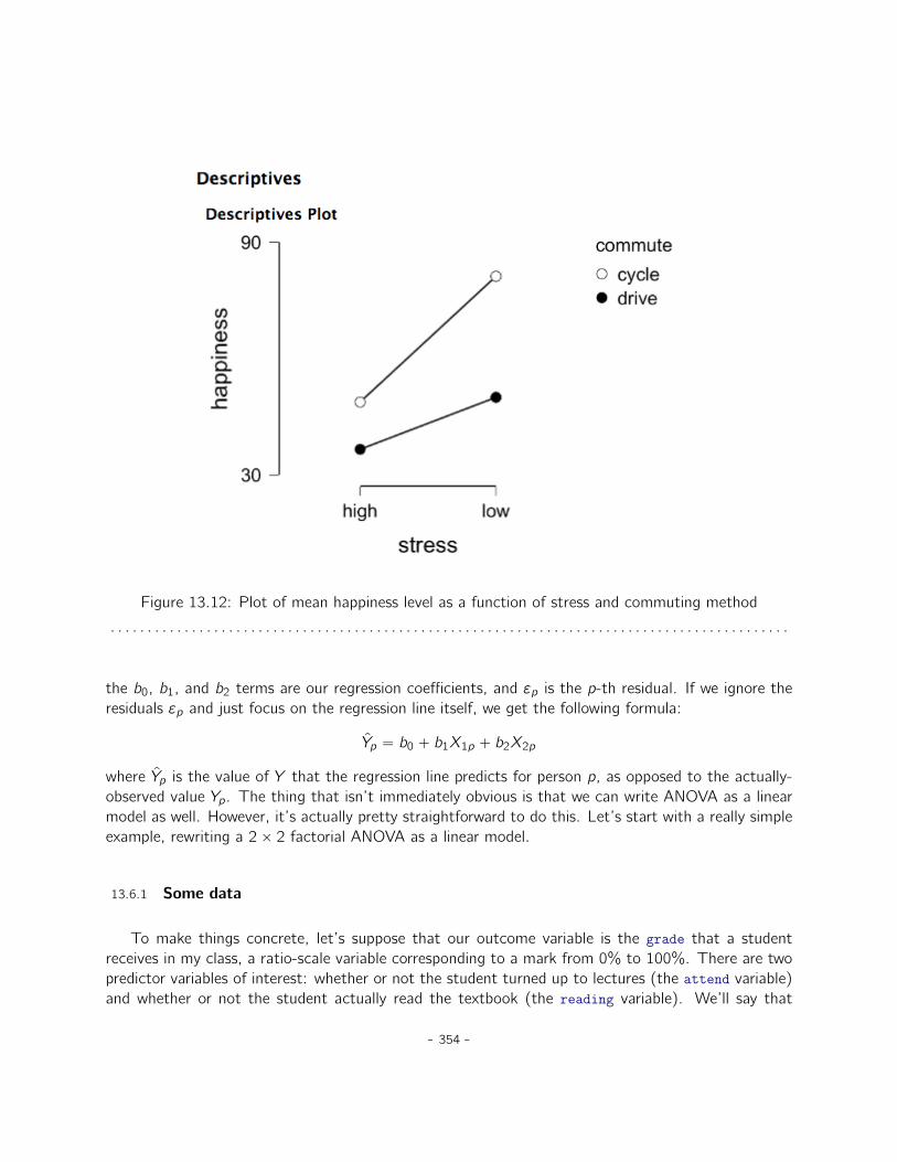
Figure 13.12: Plot of mean happiness level as a function of stress and commuting method

. . . . . . . . . . . . . . . . . . . . . . . . . . . . . . . . . . . . . . . . . . . . . . . . . . . . . . . . . . . . . . . . . . . . . . . . . . . . . . . . . . . . . . . . . . . .

the b0, b1, and b2 terms are our regression coefficients, and εp is the p-th residual. If we ignore theresiduals εp and just focus on the regression line itself, we get the following formula:

Yp “ b0 ` b1X1p ` b2X2p

where Yp is the value of Y that the regression line predicts for person p, as opposed to the actually-observed value Yp. The thing that isn’t immediately obvious is that we can write ANOVA as a linearmodel as well. However, it’s actually pretty straightforward to do this. Let’s start with a really simpleexample, rewriting a 2ˆ 2 factorial ANOVA as a linear model.

13.6.1 Some data

To make things concrete, let’s suppose that our outcome variable is the grade that a studentreceives in my class, a ratio-scale variable corresponding to a mark from 0% to 100%. There are twopredictor variables of interest: whether or not the student turned up to lectures (the attend variable)and whether or not the student actually read the textbook (the reading variable). We’ll say that

- 354 -

attend = 1 if the student attended class, and attend = 0 if they did not. Similarly, we’ll say thatreading = 1 if the student read the textbook, and reading = 0 if they did not.

Okay, so far that’s simple enough. The next thing we need to do is to wrap some maths aroundthis (sorry!). For the purposes of this example, let Yp denote the grade of the p-th student in theclass. This is not quite the same notation that we used earlier in this chapter. Previously, we’ve usedthe notation Yrci to refer to the i-th person in the r -th group for predictor 1 (the row factor) and thec-th group for predictor 2 (the column factor). This extended notation was really handy for describinghow the SS values are calculated, but it’s a pain in the current context, so I’ll switch notation here.Now, the Yp notation is visually simpler than Yrci , but it has the shortcoming that it doesn’t actuallykeep track of the group memberships! That is, if I told you that Y0,0,3 “ 35, you’d immediately knowthat we’re talking about a student (the 3rd such student, in fact) who didn’t attend the lectures (i.e.,attend = 0) and didn’t read the textbook (i.e. reading = 0), and who ended up failing the class(grade = 35). But if I tell you that Yp “ 35, all you know is that the p-th student didn’t get a goodgrade. We’ve lost some key information here. Of course, it doesn’t take a lot of thought to figureout how to fix this. What we’ll do instead is introduce two new variables X1p and X2p that keep trackof this information. In the case of our hypothetical student, we know that X1p “ 0 (i.e., attend = 0)and X2p “ 0 (i.e., reading = 0). So the data might look like this:

person, p grade, Yp attendance, X1p reading, X2p

1 90 1 12 87 1 13 75 0 14 60 1 05 35 0 06 50 0 07 65 1 08 70 0 1

This isn’t anything particularly special, of course. It’s exactly the format in which we expect to seeour data! See the data file rtfm.csv.

13.6.2 ANOVA with binary factors as a regression model

Okay, let’s get back to talking about the mathematics. We now have our data expressed in termsof three numeric variables: the continuous variable Y and the two binary variables X1 and X2. What Iwant you to recognise is that our 2ˆ2 factorial ANOVA is exactly equivalent to the regression model

Yp “ b0 ` b1X1p ` b2X2p ` εp

This is, of course, the exact same equation that I used earlier to describe a two-predictor regressionmodel! The only difference is that X1 and X2 are now binary variables (i.e., values can only be 0 or1), whereas in a regression analysis we expect that X1 and X2 will be continuous. There’s a couple

- 355 -

of ways I could try to convince you of this. One possibility would be to do a lengthy mathematicalexercise proving that the two are identical. However, I’m going to go out on a limb and guess thatmost of the readership of this book will find that annoying rather than helpful. Instead, I’ll explain thebasic ideas and then rely on JASP to show that ANOVA analyses and regression analyses aren’t justsimilar, they’re identical for all intents and purposes. Let’s start by running this as an ANOVA. To dothis, we’ll use the rtfm data set, and Figure 13.13 shows what we get when we run the analysis inJASP.

Figure 13.13: ANOVA of the rtfm.csv data set in JASP, without the interaction term

. . . . . . . . . . . . . . . . . . . . . . . . . . . . . . . . . . . . . . . . . . . . . . . . . . . . . . . . . . . . . . . . . . . . . . . . . . . . . . . . . . . . . . . . . . . .

So, by reading the key numbers off the ANOVA table and the mean scores that we presented earlier,we can see that the students obtained a higher grade if they attended class pF1,5 “ 21.6, p “ .006q

and if they read the textbook pF1,5 “ 52.3, p ă 0.001q. Let’s make a note of those p-values andthose F statistics.

Now let’s think about the same analysis from a linear regression perspective. In the rtfm dataset, we have encoded attend and reading as if they were numeric predictors. In this case, this isperfectly acceptable. There really is a sense in which a student who turns up to class (i.e. attend =1) has in fact done “more attendance” than a student who does not (i.e. attend = 0). So it’s notat all unreasonable to include it as a predictor in a regression model. It’s a little unusual, becausethe predictor only takes on two possible values, but it doesn’t violate any of the assumptions of linearregression. And it’s easy to interpret. If the regression coefficient for attend is greater than 0 it meansthat students that attend lectures get higher grades. If it’s less than zero then students attendinglectures get lower grades. The same is true for our reading variable.

Wait a second though. Why is this true? It’s something that is intuitively obvious to everyone whohas taken a few stats classes and is comfortable with the maths, but it isn’t clear to everyone else atfirst pass. To see why this is true, it helps to look closely at a few specific students. Let’s start byconsidering the 6th and 7th students in our data set (i.e. p “ 6 and p “ 7). Neither one has read thetextbook, so in both cases we can set reading = 0. Or, to say the same thing in our mathematicalnotation, we observe X2,6 “ 0 and X2,7 “ 0. However, student number 7 did turn up to lectures (i.e.,attend = 1, X1,7 “ 1) whereas student number 6 did not (i.e., attend = 0, X1,6 “ 0). Now let’s lookat what happens when we insert these numbers into the general formula for our regression line. For

- 356 -

student number 6, the regression predicts that

Y6 “ b0 ` b1X1,6 ` b2X2,6

“ b0 ` pb1 ˆ 0q ` pb2 ˆ 0q

“ b0

So we’re expecting that this student will obtain a grade corresponding to the value of the interceptterm b0. What about student 7? This time when we insert the numbers into the formula for theregression line, we obtain the following

Y7 “ b0 ` b1X1,7 ` b2X2,7

“ b0 ` pb1 ˆ 1q ` pb2 ˆ 0q

“ b0 ` b1

Because this student attended class, the predicted grade is equal to the intercept term b0 plus thecoefficient associated with the attend variable, b1. So, if b1 is greater than zero, we’re expecting thatthe students who turn up to lectures will get higher grades than those students who don’t. If thiscoefficient is negative we’re expecting the opposite: students who turn up at class end up performingmuch worse. In fact, we can push this a little bit further. What about student number 1, who turnedup to class (X1,1 “ 1) and read the textbook (X2,1 “ 1)? If we plug these numbers into the regressionwe get

Y1 “ b0 ` b1X1,1 ` b2X2,1

“ b0 ` pb1 ˆ 1q ` pb2 ˆ 1q

“ b0 ` b1 ` b2

So if we assume that attending class helps you get a good grade (i.e., b1 ą 0) and if we assumethat reading the textbook also helps you get a good grade (i.e., b2 ą 0), then our expectation is thatstudent 1 will get a grade that that is higher than student 6 and student 7.

And at this point you won’t be at all suprised to learn that the regression model predicts thatstudent 3, who read the book but didn’t attend lectures, will obtain a grade of b2 ` b0. I won’tbore you with yet another regression formula. Instead, what I’ll do is show you the following table ofexpected grades:

read textbook?no yes

attended? no b0 b0 ` b2

yes b0 ` b1 b0 ` b1 ` b2

As you can see, the intercept term b0 acts like a kind of “baseline” grade that you would expect fromthose students who don’t take the time to attend class or read the textbook. Similarly, b1 representsthe boost that you’re expected to get if you come to class, and b2 represents the boost that comes

- 357 -

from reading the textbook. In fact, if this were an ANOVA you might very well want to characteriseb1 as the main effect of attendance, and b2 as the main effect of reading! In fact, for a simple 2ˆ 2

ANOVA that’s exactly how it plays out.

Okay, now that we’re really starting to see why ANOVA and regression are basically the samething, let’s actually run our regression using the rtfm data and the JASP regression analysis toconvince ourselves that this is really true. Running the regression in the usual way gives the resultsshown in Figure 13.14.

Figure 13.14: Regression analysis of the rtfm.csv data set in JASP, without the interaction term

. . . . . . . . . . . . . . . . . . . . . . . . . . . . . . . . . . . . . . . . . . . . . . . . . . . . . . . . . . . . . . . . . . . . . . . . . . . . . . . . . . . . . . . . . . . .

There’s a few interesting things to note here. First, notice that the intercept term is 43.5 which isclose to the “group” mean of 42.5 observed for those two students who didn’t read the text or attendclass. Second, notice that we have the regression coefficient of b1 “ 18.0 for the attendance variable,suggesting that those students that attended class scored 18 points higher than those who didn’t. Soour expectation would be that those students who turned up to class but didn’t read the textbookwould obtain a grade of b0 ` b1, which is equal to 43.5 ` 18.0 “ 61.5. You can verify for yourselfthat the same thing happens when we look at the students that read the textbook.

Actually, we can push a little further in establishing the equivalence of our ANOVA and our re-gression. Look at the p-values associated with the attend variable and the reading variable in theregression output. They’re identical to the ones we encountered earlier when running the ANOVA.This might seem a little surprising, since the test used when running our regression model calculates at-statistic and the ANOVA calculates an F -statistic. However, if you can remember all the way backto Chapter 6, I mentioned that there’s a relationship between the t-distribution and the F -distribution.If you have some quantity that is distributed according to a t-distribution with k degrees of freedomand you square it, then this new squared quantity follows an F -distribution whose degrees of freedomare 1 and k . We can check this with respect to the t statistics in our regression model. For the attendvariable we get a t value of 4.65. If we square this number we end up with 21.6, which matches thecorresponding F statistic in our ANOVA.

13.6.3 Using contrasts to encode non binary factors

At this point, I’ve shown you how we can view a 2ˆ 2 ANOVA into a linear model. And it’s pretty

- 358 -

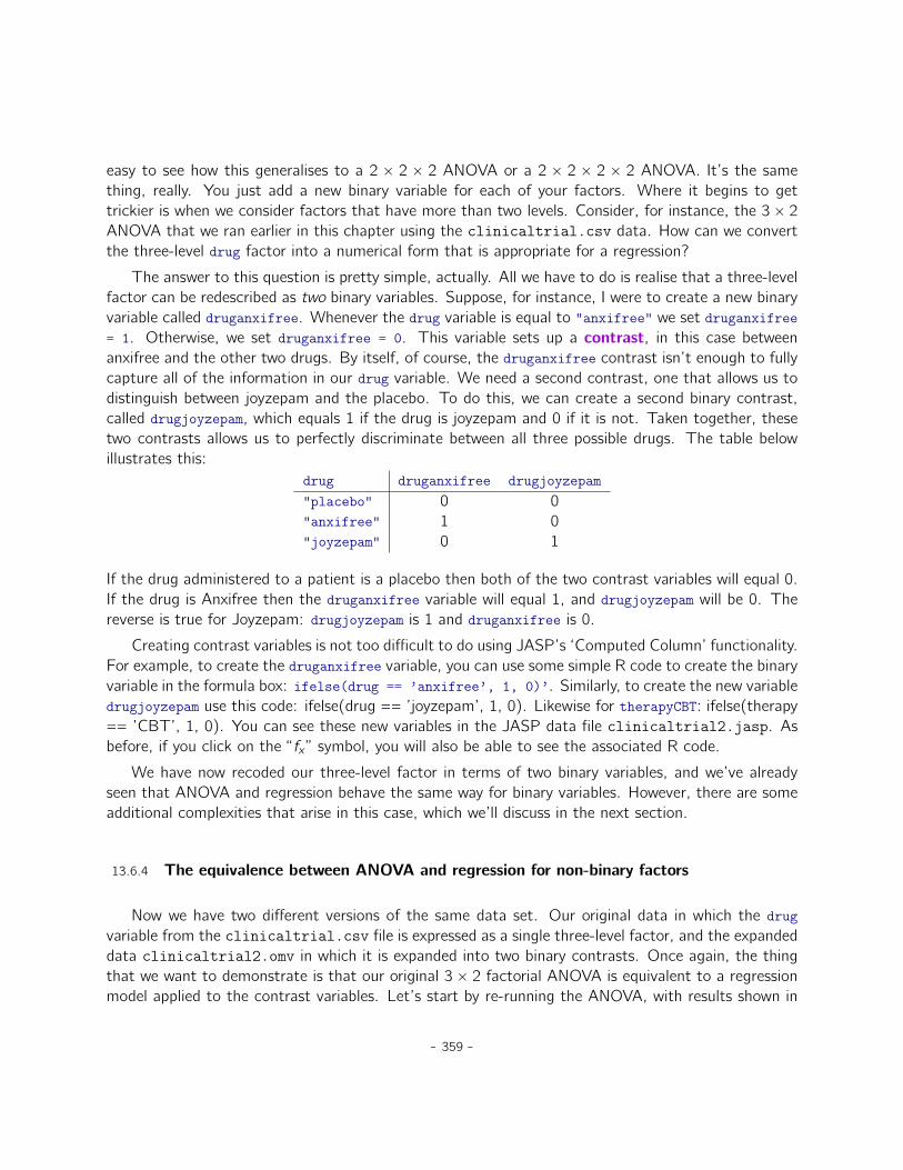
easy to see how this generalises to a 2 ˆ 2 ˆ 2 ANOVA or a 2 ˆ 2 ˆ 2 ˆ 2 ANOVA. It’s the samething, really. You just add a new binary variable for each of your factors. Where it begins to gettrickier is when we consider factors that have more than two levels. Consider, for instance, the 3ˆ 2

ANOVA that we ran earlier in this chapter using the clinicaltrial.csv data. How can we convertthe three-level drug factor into a numerical form that is appropriate for a regression?

The answer to this question is pretty simple, actually. All we have to do is realise that a three-levelfactor can be redescribed as two binary variables. Suppose, for instance, I were to create a new binaryvariable called druganxifree. Whenever the drug variable is equal to "anxifree" we set druganxifree= 1. Otherwise, we set druganxifree = 0. This variable sets up a contrast, in this case betweenanxifree and the other two drugs. By itself, of course, the druganxifree contrast isn’t enough to fullycapture all of the information in our drug variable. We need a second contrast, one that allows us todistinguish between joyzepam and the placebo. To do this, we can create a second binary contrast,called drugjoyzepam, which equals 1 if the drug is joyzepam and 0 if it is not. Taken together, thesetwo contrasts allows us to perfectly discriminate between all three possible drugs. The table belowillustrates this:

drug druganxifree drugjoyzepam"placebo" 0 0"anxifree" 1 0"joyzepam" 0 1

If the drug administered to a patient is a placebo then both of the two contrast variables will equal 0.If the drug is Anxifree then the druganxifree variable will equal 1, and drugjoyzepam will be 0. Thereverse is true for Joyzepam: drugjoyzepam is 1 and druganxifree is 0.

Creating contrast variables is not too difficult to do using JASP’s ‘Computed Column’ functionality.For example, to create the druganxifree variable, you can use some simple R code to create the binaryvariable in the formula box: ifelse(drug == ’anxifree’, 1, 0)’. Similarly, to create the new variabledrugjoyzepam use this code: ifelse(drug == ’joyzepam’, 1, 0). Likewise for therapyCBT: ifelse(therapy== ’CBT’, 1, 0). You can see these new variables in the JASP data file clinicaltrial2.jasp. Asbefore, if you click on the “fx ” symbol, you will also be able to see the associated R code.

We have now recoded our three-level factor in terms of two binary variables, and we’ve alreadyseen that ANOVA and regression behave the same way for binary variables. However, there are someadditional complexities that arise in this case, which we’ll discuss in the next section.

13.6.4 The equivalence between ANOVA and regression for non-binary factors

Now we have two different versions of the same data set. Our original data in which the drugvariable from the clinicaltrial.csv file is expressed as a single three-level factor, and the expandeddata clinicaltrial2.omv in which it is expanded into two binary contrasts. Once again, the thingthat we want to demonstrate is that our original 3ˆ 2 factorial ANOVA is equivalent to a regressionmodel applied to the contrast variables. Let’s start by re-running the ANOVA, with results shown in

- 359 -

Figure 13.15. Let’s remove the interaction component; remember to go to ‘Model’ and move thedrug*therapy term out of the ‘Model Terms’ box.

Figure 13.15: JASP ANOVA results, without interaction component

. . . . . . . . . . . . . . . . . . . . . . . . . . . . . . . . . . . . . . . . . . . . . . . . . . . . . . . . . . . . . . . . . . . . . . . . . . . . . . . . . . . . . . . . . . . .

Obviously, there are no surprises here. That’s the exact same ANOVA that we ran earlier. Next,let’s run a regression using druganxifree, drugjoyzepam and CBTtherapy as the predictors. The resultsare shown in Figure 13.16.

Figure 13.16: JASP regression results, with contrast variables druganxifree and drugjoyzepam

. . . . . . . . . . . . . . . . . . . . . . . . . . . . . . . . . . . . . . . . . . . . . . . . . . . . . . . . . . . . . . . . . . . . . . . . . . . . . . . . . . . . . . . . . . . .

Hmm. This will look quite different than what we got last time. Not surprisingly, the regressionoutput prints out the results for each of the three predictors separately, just like it did every other timewe conducted a regression analysis. On the one hand we can see that the p-value for the CBTtherapyvariable is exactly the same as the one for the therapy factor in our original ANOVA, so we can bereassured that the regression model is doing the same thing as the ANOVA did. On the other hand,this regression model is testing the druganxifree contrast and the drugjoyzepam contrast separately,as if they were two completely unrelated variables. It’s not surprising of course, because the poorregression analysis has no way of knowing that drugjoyzepam and druganxifree are actually the twodifferent contrasts that we used to encode our three-level drug factor. As far as it knows, drugjoyzepamand druganxifree are no more related to one another than drugjoyzepam and therapyCBT. However,you and I know better. At this stage we’re not at all interested in determining whether these two

- 360 -

contrasts are individually significant. We just want to know if there’s an “overall” effect of drug. Thatis, what we want JASP to do is to run some kind of “model comparison” test, one in which the two“drug-related” contrasts are lumped together for the purpose of the test. Sound familiar? All we needto do is specify a “null model”, which in this case would include the CBTtherapy predictor, and omitboth of the drug-related variables, as in Figure 13.17. To do this, click the ‘Model’ button and check‘Add to null model’ for both of the drug terms. You can then assess whether to include drug as apredictor in the model by computing AIC for both models (see Section 11.11). Remember, smaller isbetter!

13.7

Different ways to specify contrasts

In the previous section, I showed you a method for converting a factor into a collection of contrasts.In the method I showed you we specify a set of binary variables in which we defined a table like thisone:

drug druganxifree drugjoyzepam"placebo" 0 0"anxifree" 1 0"joyzepam" 0 1

Each row in the table corresponds to one of the factor levels, and each column corresponds to oneof the contrasts. This table, which always has one more row than columns, has a special name. It iscalled a contrast matrix. However, there are lots of different ways to specify a contrast matrix. In thissection I discuss a few of the standard contrast matrices that statisticians use and how you can usethem in JASP. If you’re planning to read the section on unbalanced ANOVA later on (Section 13.10),it’s worth reading this section carefully. If not, you can get away with skimming it, because the choiceof contrasts doesn’t matter much for balanced designs.

13.7.1 Treatment contrasts

In the particular kind of contrasts that I’ve described above, one level of the factor is special,and acts as a kind of “baseline” category (i.e., placebo in our example), against which the other twoare defined. The name for these kinds of contrasts is treatment contrasts, also known as “dummycoding”. In this contrast each level of the factor is compared to a base reference level, and the basereference level is the value of the intercept.

The name reflects the fact that these contrasts are quite natural and sensible when one of thecategories in your factor really is special because it actually does represent a baseline. That makessense in our clinical trial example. The placebo condition corresponds to the situation where you don’t

- 361 -

Figure 13.17: Model comparison in JASP regression, null model 0 vs. contrasts model 1

. . . . . . . . . . . . . . . . . . . . . . . . . . . . . . . . . . . . . . . . . . . . . . . . . . . . . . . . . . . . . . . . . . . . . . . . . . . . . . . . . . . . . . . . . . . .

- 362 -

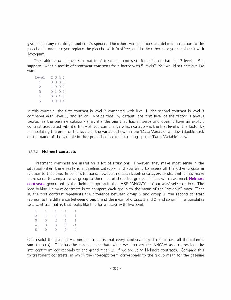
give people any real drugs, and so it’s special. The other two conditions are defined in relation to theplacebo. In one case you replace the placebo with Anxifree, and in the other case your replace it withJoyzepam.

The table shown above is a matrix of treatment contrasts for a factor that has 3 levels. Butsuppose I want a matrix of treatment contrasts for a factor with 5 levels? You would set this out likethis:

Level 2 3 4 51 0 0 0 02 1 0 0 03 0 1 0 04 0 0 1 05 0 0 0 1

In this example, the first contrast is level 2 compared with level 1, the second contrast is level 3compared with level 1, and so on. Notice that, by default, the first level of the factor is alwaystreated as the baseline category (i.e., it’s the one that has all zeros and doesn’t have an explicitcontrast associated with it). In JASP you can change which category is the first level of the factor bymanipulating the order of the levels of the variable shown in the ‘Data Variable’ window (double clickon the name of the variable in the spreadsheet column to bring up the ‘Data Variable’ view.

13.7.2 Helmert contrasts

Treatment contrasts are useful for a lot of situations. However, they make most sense in thesituation when there really is a baseline category, and you want to assess all the other groups inrelation to that one. In other situations, however, no such baseline category exists, and it may makemore sense to compare each group to the mean of the other groups. This is where we meet Helmertcontrasts, generated by the ‘helmert’ option in the JASP ‘ANOVA’ - ‘Contrasts’ selection box. Theidea behind Helmert contrasts is to compare each group to the mean of the “previous” ones. Thatis, the first contrast represents the difference between group 2 and group 1, the second contrastrepresents the difference between group 3 and the mean of groups 1 and 2, and so on. This translatesto a contrast matrix that looks like this for a factor with five levels:

1 -1 -1 -1 -12 1 -1 -1 -13 0 2 -1 -14 0 0 3 -15 0 0 0 4

One useful thing about Helmert contrasts is that every contrast sums to zero (i.e., all the columnssum to zero). This has the consequence that, when we interpret the ANOVA as a regression, theintercept term corresponds to the grand mean µ.. if we are using Helmert contrasts. Compare thisto treatment contrasts, in which the intercept term corresponds to the group mean for the baseline

- 363 -

category. This property can be very useful in some situations. It doesn’t matter very much if you havea balanced design, which we’ve been assuming so far, but it will turn out to be important later whenwe consider unbalanced designs in Section 13.10. In fact, the main reason why I’ve even bothered toinclude this section is that contrasts become important if you want to understand unbalanced ANOVA.

13.7.3 Sum to zero contrasts

The third option that I should briefly mention are “sum to zero” contrasts, called “Simple” con-trasts in JASP, which are used to construct pairwise comparisons between groups. Specifically, eachcontrast encodes the difference between one of the groups and a baseline category, which in this casecorresponds to the first group:

1 -1 -1 -1 -12 1 0 0 03 0 1 0 04 0 0 1 05 0 0 0 1

Much like Helmert contrasts, we see that each column sums to zero, which means that the interceptterm corresponds to the grand mean when ANOVA is treated as a regression model. When interpretingthese contrasts, the thing to recognise is that each of these contrasts is a pairwise comparison betweengroup 1 and one of the other four groups. Specifically, contrast 1 corresponds to a “group 2 minusgroup 1” comparison, contrast 2 corresponds to a “group 3 minus group 1” comparison, and so on.6

13.7.4 Optional contrasts in JASP

JASP also comes with a variety of options that can generate different kinds of contrasts in ANOVA.These can be found in the ‘Contrasts’ option in the main ANOVA analysis window, where the followingcontrast types are listed:

6What’s the difference between treatment and simple contrasts, I hear you ask? Well, as a basic example considera gender main effect, with m=0 and f=1. The coefficient corresponding to the treatment contrast will measure thedifference in mean between females and males, and the intercept would be the mean of the males. However, with asimple contrast, i.e., m=-1 and f=1, the intercept is the average of the means and the main effect is the difference ofeach group mean from the intercept.

- 364 -

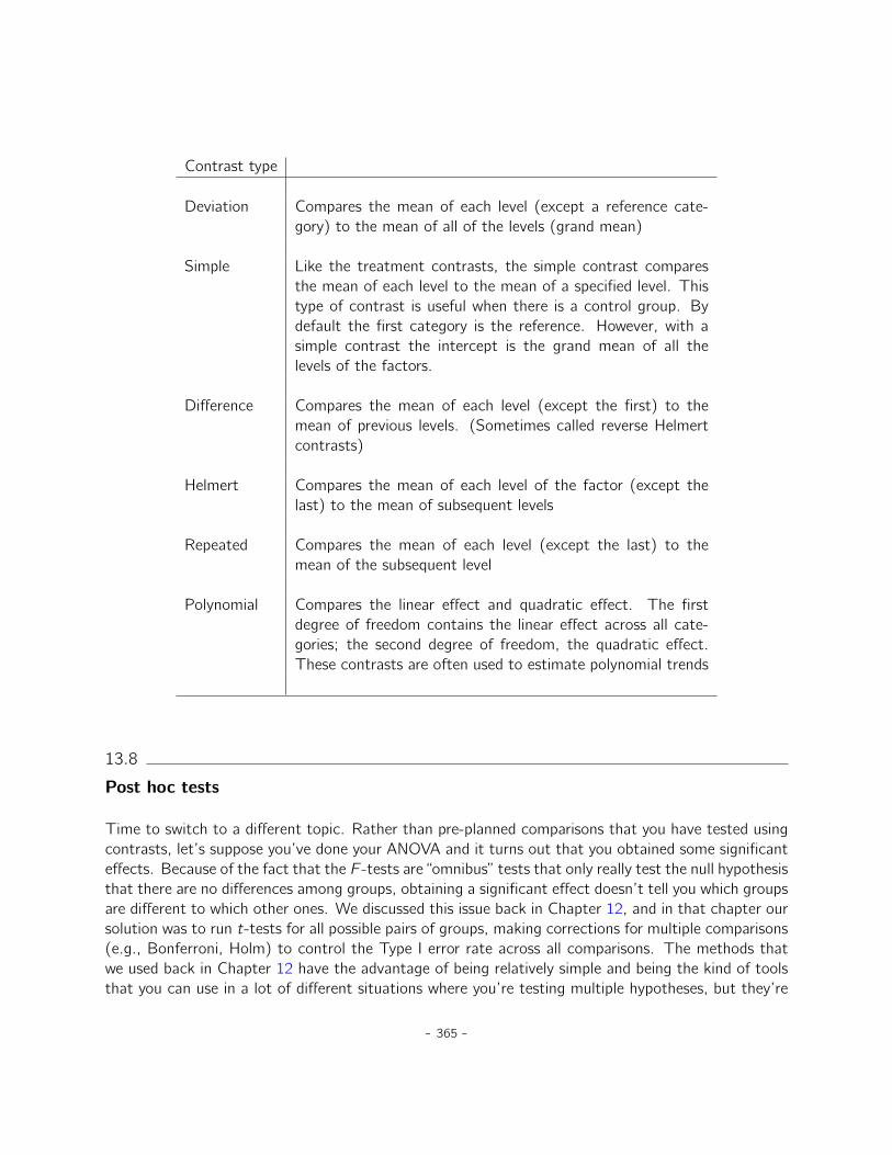
Contrast type

Deviation Compares the mean of each level (except a reference cate-gory) to the mean of all of the levels (grand mean)

Simple Like the treatment contrasts, the simple contrast comparesthe mean of each level to the mean of a specified level. Thistype of contrast is useful when there is a control group. Bydefault the first category is the reference. However, with asimple contrast the intercept is the grand mean of all thelevels of the factors.

Difference Compares the mean of each level (except the first) to themean of previous levels. (Sometimes called reverse Helmertcontrasts)

Helmert Compares the mean of each level of the factor (except thelast) to the mean of subsequent levels

Repeated Compares the mean of each level (except the last) to themean of the subsequent level

Polynomial Compares the linear effect and quadratic effect. The firstdegree of freedom contains the linear effect across all cate-gories; the second degree of freedom, the quadratic effect.These contrasts are often used to estimate polynomial trends

13.8

Post hoc tests

Time to switch to a different topic. Rather than pre-planned comparisons that you have tested usingcontrasts, let’s suppose you’ve done your ANOVA and it turns out that you obtained some significanteffects. Because of the fact that the F -tests are “omnibus” tests that only really test the null hypothesisthat there are no differences among groups, obtaining a significant effect doesn’t tell you which groupsare different to which other ones. We discussed this issue back in Chapter 12, and in that chapter oursolution was to run t-tests for all possible pairs of groups, making corrections for multiple comparisons(e.g., Bonferroni, Holm) to control the Type I error rate across all comparisons. The methods thatwe used back in Chapter 12 have the advantage of being relatively simple and being the kind of toolsthat you can use in a lot of different situations where you’re testing multiple hypotheses, but they’re

- 365 -

not necessarily the best choices if you’re interested in doing efficient post hoc testing in an ANOVAcontext. There are actually quite a lot of different methods for performing multiple comparisons inthe statistics literature (Hsu 1996), and it would be beyond the scope of an introductory text like thisone to discuss all of them in any detail.

That being said, there’s one tool that I do want to draw your attention to, namely Tukey’s“Honestly Significant Difference”, or Tukey’s HSD for short. For once, I’ll spare you the formulas andjust stick to the qualitative ideas. The basic idea in Tukey’s HSD is to examine all relevant pairwisecomparisons between groups, and it’s only really appropriate to use Tukey’s HSD if it is pairwisedifferences that you’re interested in.7 For instance, earlier we conducted a factorial ANOVA using theclinicaltrial.csv data set, and where we specified a main effect for drug and a main effect oftherapy we would be interested in the following four comparisons:

• The difference in mood gain for people given Anxifree versus people given the placebo.

• The difference in mood gain for people given Joyzepam versus people given the placebo.

• The difference in mood gain for people given Anxifree versus people given Joyzepam.

• The difference in mood gain for people treated with CBT and people given no therapy.

For any one of these comparisons, we’re interested in the true difference between (population) groupmeans. Tukey’s HSD constructs simultaneous confidence intervals for all four of these comparisons.What we mean by 95% “simultaneous” confidence interval is that, if we were to repeat this study manytimes, then in 95% of the study results the confidence intervals would contain the relevant true value.Moreover, we can use these confidence intervals to calculate an adjusted p value for any specificcomparison.

The TukeyHSD function in JASP is pretty easy to use. You simply specify the ANOVA model termthat you want to run the post hoc tests for. For example, if we were looking to run post hoc testsfor the main effects but not the interaction, we would open up the ‘Post Hoc Tests’ option in theANOVA analysis screen, move the drug and therapy variables across to the box on the right, and thenselect the ‘Tukey’ checkbox in the list of possible post hoc corrections that could be applied. This,along with the corresponding results table, is shown in Figure 13.18

The output shown in the ‘Post Hoc Tests’ results table is (I hope) pretty straightforward. The firstcomparison, for example, is the Anxifree versus placebo difference, and the first part of the outputindicates that the observed difference in group means is .27. The next number is the standard errorfor the difference, from which we could calculate the 95% confidence interval (you can actually displaythis 95% CI if you select the ‘Confidence intervals’ box). Then there is a column with the degrees offreedom, a column with the t-value, and finally a column with the p-value. For the first comparison

7If, for instance, you actually find yourself interested to know if Group A is significantly different from the mean ofGroup B and Group C, then you need to use a different tool (e.g., Scheffe’s method, which is more conservative, andbeyond the scope of this book). However, in most cases you probably are interested in pairwise group differences, soTukey’s HSD is a pretty useful thing to know about.

- 366 -

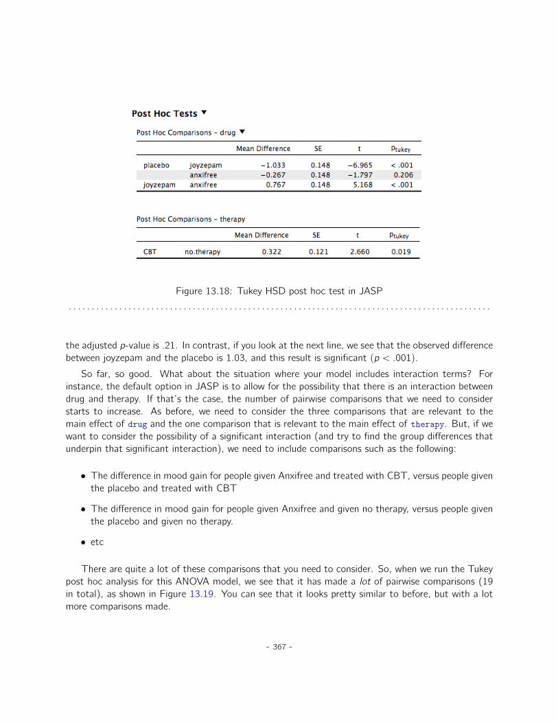
Figure 13.18: Tukey HSD post hoc test in JASP

. . . . . . . . . . . . . . . . . . . . . . . . . . . . . . . . . . . . . . . . . . . . . . . . . . . . . . . . . . . . . . . . . . . . . . . . . . . . . . . . . . . . . . . . . . . .

the adjusted p-value is .21. In contrast, if you look at the next line, we see that the observed differencebetween joyzepam and the placebo is 1.03, and this result is significant pp ă .001q.

So far, so good. What about the situation where your model includes interaction terms? Forinstance, the default option in JASP is to allow for the possibility that there is an interaction betweendrug and therapy. If that’s the case, the number of pairwise comparisons that we need to considerstarts to increase. As before, we need to consider the three comparisons that are relevant to themain effect of drug and the one comparison that is relevant to the main effect of therapy. But, if wewant to consider the possibility of a significant interaction (and try to find the group differences thatunderpin that significant interaction), we need to include comparisons such as the following:

• The difference in mood gain for people given Anxifree and treated with CBT, versus people giventhe placebo and treated with CBT

• The difference in mood gain for people given Anxifree and given no therapy, versus people giventhe placebo and given no therapy.

• etc

There are quite a lot of these comparisons that you need to consider. So, when we run the Tukeypost hoc analysis for this ANOVA model, we see that it has made a lot of pairwise comparisons (19in total), as shown in Figure 13.19. You can see that it looks pretty similar to before, but with a lotmore comparisons made.

- 367 -

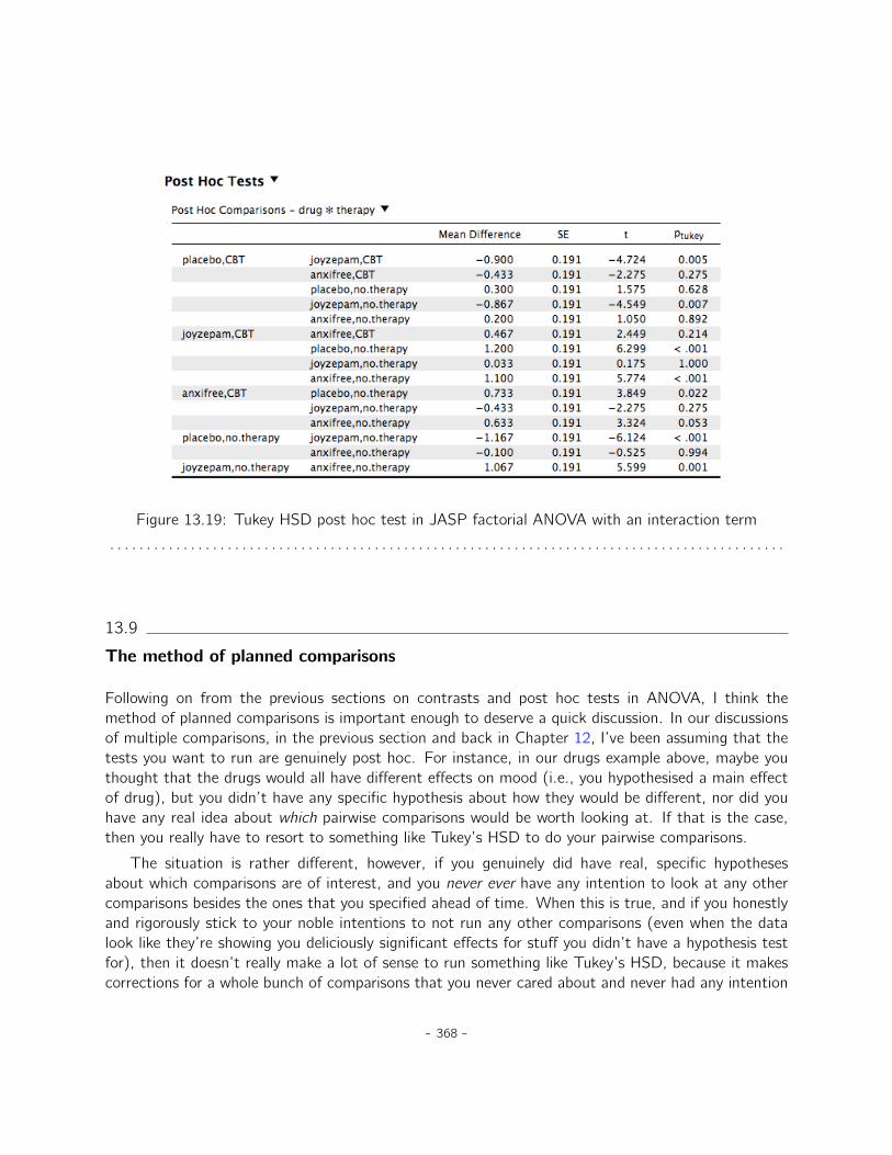
Figure 13.19: Tukey HSD post hoc test in JASP factorial ANOVA with an interaction term

. . . . . . . . . . . . . . . . . . . . . . . . . . . . . . . . . . . . . . . . . . . . . . . . . . . . . . . . . . . . . . . . . . . . . . . . . . . . . . . . . . . . . . . . . . . .

13.9

The method of planned comparisons

Following on from the previous sections on contrasts and post hoc tests in ANOVA, I think themethod of planned comparisons is important enough to deserve a quick discussion. In our discussionsof multiple comparisons, in the previous section and back in Chapter 12, I’ve been assuming that thetests you want to run are genuinely post hoc. For instance, in our drugs example above, maybe youthought that the drugs would all have different effects on mood (i.e., you hypothesised a main effectof drug), but you didn’t have any specific hypothesis about how they would be different, nor did youhave any real idea about which pairwise comparisons would be worth looking at. If that is the case,then you really have to resort to something like Tukey’s HSD to do your pairwise comparisons.

The situation is rather different, however, if you genuinely did have real, specific hypothesesabout which comparisons are of interest, and you never ever have any intention to look at any othercomparisons besides the ones that you specified ahead of time. When this is true, and if you honestlyand rigorously stick to your noble intentions to not run any other comparisons (even when the datalook like they’re showing you deliciously significant effects for stuff you didn’t have a hypothesis testfor), then it doesn’t really make a lot of sense to run something like Tukey’s HSD, because it makescorrections for a whole bunch of comparisons that you never cared about and never had any intention

- 368 -

of looking at. Under those circumstances, you can safely run a (limited) number of hypothesis testswithout making an adjustment for multiple testing. This situation is known as the method of plannedcomparisons, and it is sometimes used in clinical trials. However, further consideration is out of scopefor this introductory book, but at least you know that this method exists!

13.10

Factorial ANOVA 3: unbalanced designs

Factorial ANOVA is a very handy thing to know about. It’s been one of the standard tools used toanalyse experimental data for many decades, and you’ll find that you can’t read more than two orthree papers in psychology without running into an ANOVA in there somewhere. However, there’sone huge difference between the ANOVAs that you’ll see in a lot of real scientific articles and theANOVAs that I’ve described so far. In in real life we’re rarely lucky enough to have perfectly balanceddesigns. For one reason or another, it’s typical to end up with more observations in some cells thanin others. Or, to put it another way, we have an unbalanced design.

Unbalanced designs need to be treated with a lot more care than balanced designs, and thestatistical theory that underpins them is a lot messier. It might be a consequence of this messiness,or it might be a shortage of time, but my experience has been that undergraduate research methodsclasses in psychology have a nasty tendency to ignore this issue completely. A lot of stats textbookstend to gloss over it too. The net result of this, I think, is that a lot of active researchers in the fielddon’t actually know that there’s several different “types” of unbalanced ANOVAs, and they producequite different answers. In fact, reading the psychological literature, I’m kind of amazed at the factthat most people who report the results of an unbalanced factorial ANOVA don’t actually give youenough details to reproduce the analysis. I secretly suspect that most people don’t even realise thattheir statistical software package is making a whole lot of substantive data analysis decisions on theirbehalf. It’s actually a little terrifying when you think about it. So, if you want to avoid handing controlof your data analysis to stupid software, read on.

13.10.1 The coffee data

As usual, it will help us to work with some data. The coffee.csv file contains a hypothetical dataset that produces an unbalanced 3ˆ 2 ANOVA. Suppose we were interested in finding out whether ornot the tendency of people to babble when they have too much coffee is purely an effect of the coffeeitself, or whether there’s some effect of the milk and sugar that people add to the coffee. Supposewe took 18 people and gave them some coffee to drink. The amount of coffee / caffeine was heldconstant, and we varied whether or not milk was added, so milk is a binary factor with two levels,"yes" and "no". We also varied the kind of sugar involved. The coffee might contain "real" sugaror it might contain "fake" sugar (i.e., artificial sweetener) or it might contain "none" at all, so the

- 369 -

sugar variable is a three level factor. Our outcome variable is a continuous variable that presumablyrefers to some psychologically sensible measure of the extent to which someone is “babbling”. Thedetails don’t really matter for our purpose. Take a look at the data in the JASP spreadsheet view, asin Figure 13.20.

Looking at the table of means in Figure 13.20 we get a strong impression that there are differencesbetween the groups. This is especially true when we look at the standard deviations. Across groups,this standard deviation varies quite a lot.8 Whilst this at first may seem like a straightforward factorialANOVA, a problem arises when we look at how many observations we have in each group. See thedifferent Ns for different groups shown in Figure 13.20. This violates one of our original assumptions,namely that the number of people in each group is the same. We haven’t really discussed how tohandle this situation.

13.10.2 “Standard ANOVA” does not exist for unbalanced designs

Unbalanced designs lead us to the somewhat unsettling discovery that there isn’t really any onething that we might refer to as a standard ANOVA. In fact, it turns out that there are three funda-mentally different ways9 in which you might want to run an ANOVA in an unbalanced design. If youhave a balanced design all three versions produce identical results, with the sums of squares, F -values,etc., all conforming to the formulas that I gave at the start of the chapter. However, when your designis unbalanced they don’t give the same answers. Furthermore, they are not all equally appropriate toevery situation. Some methods will be more appropriate to your situation than others. Given all this,it’s important to understand what the different types of ANOVA are and how they differ from oneanother.

The first kind of ANOVA is conventionally referred to as Type I sum of squares. I’m sure youcan guess what the other two are called. The “sum of squares” part of the name was introduced bythe SAS statistical software package and has become standard nomenclature, but it’s a bit misleadingin some ways. I think the logic for referring to them as different types of sum of squares is that,when you look at the ANOVA tables that they produce, the key difference in the numbers is the SSvalues. The degrees of freedom don’t change, the MS values are still defined as SS divided by df,etc. However, what the terminology gets wrong is that it hides the reason why the SS values aredifferent from one another. To that end, it’s a lot more helpful to think of the three different kinds of

8This discrepancy in standard deviations might (and should) make you wonder if we have a violation of the homogeneityof variance assumption. I’ll leave it as an exercise for the reader to double check this using the Levene test option.

9Actually, this is a bit of a lie. ANOVAs can vary in other ways besides the ones I’ve discussed in this book. Forinstance, I’ve completely ignored the difference between fixed-effect models in which the levels of a factor are “fixed” bythe experimenter or the world, and random-effect models in which the levels are random samples from a larger populationof possible levels (this book only covers fixed-effect models). Don’t make the mistake of thinking that this book, or anyother one, will tell you “everything you need to know” about statistics, any more than a single book could possibly tellyou everything you need to know about psychology, physics or philosophy. Life is too complicated for that to ever betrue. This isn’t a cause for despair, though. Most researchers get by with a basic working knowledge of ANOVA thatdoesn’t go any further than this book does. I just want you to keep in mind that this book is only the beginning of avery long story, not the whole story.

- 370 -

Figure 13.20: Descriptives for the coffee.csv data set, separately split by milk and sugar, respec-tively.

. . . . . . . . . . . . . . . . . . . . . . . . . . . . . . . . . . . . . . . . . . . . . . . . . . . . . . . . . . . . . . . . . . . . . . . . . . . . . . . . . . . . . . . . . . . .

- 371 -

ANOVA as three different hypothesis testing strategies. These different strategies lead to different SSvalues, to be sure, but it’s the strategy that is the important thing here, not the SS values themselves.Recall from Section 13.6 that any particular F -test is best thought of as a comparison between twolinear models. So, when you’re looking at an ANOVA table, it helps to remember that each of thoseF -tests corresponds to a pair of models that are being compared. Of course, this leads naturally tothe question of which pair of models is being compared. This is the fundamental difference betweenANOVA Types I, II and III: each one corresponds to a different way of choosing the model pairs forthe tests.

13.10.3 Type I sum of squares

The Type I method is sometimes referred to as the “sequential” sum of squares, because it involvesa process of adding terms to the model one at a time. Consider the coffee data, for instance. Supposewe want to run the full 3ˆ2 factorial ANOVA, including interaction terms. The full model contains theoutcome variable babble, the predictor variables sugar and milk, and the interaction term sugar*milk.This can be written as babble ~ sugar + milk + sugar*milk. The Type I strategy builds this modelup sequentially, starting from the simplest possible model and gradually adding terms.

The simplest possible model for the data would be one in which neither milk nor sugar is assumedto have any effect on babbling. The only term that would be included in such a model is the intercept,written as babble ~ 1. This is our initial null hypothesis. The next simplest model for the datawould be one in which only one of the two main effects is included. In the coffee data, there are twodifferent possible choices here, because we could choose to add milk first or to add sugar first. Theorder actually turns out to matter, as we’ll see later, but for now let’s just make a choice arbitrarilyand pick sugar. So, the second model in our sequence of models is babble ~ sugar, and it forms thealternative hypothesis for our first test. We now have our first hypothesis test:

Null model: babble ~ 1Alternative model: babble ~ sugar

This comparison forms our hypothesis test of the main effect of sugar. The next step in ourmodel building exercise is to add the other main effect term, so the next model in our sequenceis babble ~ sugar + milk. The second hypothesis test is then formed by comparing the following pairof models:

Null model: babble ~ sugarAlternative model: babble ~ sugar + milk

This comparison forms our hypothesis test of the main effect of milk. In one sense, this approach isvery elegant: the alternative hypothesis from the first test forms the null hypothesis for the second one.It is in this sense that the Type I method is strictly sequential. Every test builds directly on the resultsof the last one. However, in another sense it’s very inelegant, because there’s a strong asymmetrybetween the two tests. The test of the main effect of sugar (the first test) completely ignores milk,whereas the test of the main effect of milk (the second test) does take sugar into account. In anycase, the fourth model in our sequence is now the full model, babble ~ sugar + milk + sugar*milk,

- 372 -

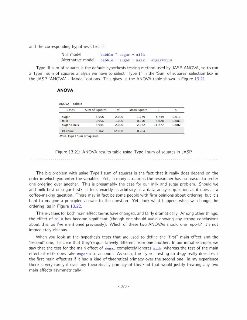
and the corresponding hypothesis test is:

Null model: babble ~ sugar + milkAlternative model: babble ~ sugar + milk + sugar*milk

Type III sum of squares is the default hypothesis testing method used by JASP ANOVA, so to runa Type I sum of squares analysis we have to select ‘Type 1’ in the ‘Sum of squares’ selection box inthe JASP ‘ANOVA’ - ‘Model’ options. This gives us the ANOVA table shown in Figure 13.21.

Figure 13.21: ANOVA results table using Type I sum of squares in JASP

. . . . . . . . . . . . . . . . . . . . . . . . . . . . . . . . . . . . . . . . . . . . . . . . . . . . . . . . . . . . . . . . . . . . . . . . . . . . . . . . . . . . . . . . . . . .

The big problem with using Type I sum of squares is the fact that it really does depend on theorder in which you enter the variables. Yet, in many situations the researcher has no reason to preferone ordering over another. This is presumably the case for our milk and sugar problem. Should weadd milk first or sugar first? It feels exactly as arbitrary as a data analysis question as it does as acoffee-making question. There may in fact be some people with firm opinions about ordering, but it’shard to imagine a principled answer to the question. Yet, look what happens when we change theordering, as in Figure 13.22.

The p-values for both main effect terms have changed, and fairly dramatically. Among other things,the effect of milk has become significant (though one should avoid drawing any strong conclusionsabout this, as I’ve mentioned previously). Which of these two ANOVAs should one report? It’s notimmediately obvious.

When you look at the hypothesis tests that are used to define the “first” main effect and the“second” one, it’s clear that they’re qualitatively different from one another. In our initial example, wesaw that the test for the main effect of sugar completely ignores milk, whereas the test of the maineffect of milk does take sugar into account. As such, the Type I testing strategy really does treatthe first main effect as if it had a kind of theoretical primacy over the second one. In my experiencethere is very rarely if ever any theoretically primacy of this kind that would justify treating any twomain effects asymmetrically.

- 373 -

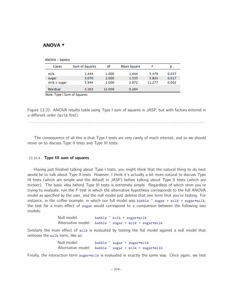
Figure 13.22: ANOVA results table using Type I sum of squares in JASP, but with factors entered ina different order (milk first)

. . . . . . . . . . . . . . . . . . . . . . . . . . . . . . . . . . . . . . . . . . . . . . . . . . . . . . . . . . . . . . . . . . . . . . . . . . . . . . . . . . . . . . . . . . . .

The consequence of all this is that Type I tests are very rarely of much interest, and so we shouldmove on to discuss Type II tests and Type III tests.

13.10.4 Type III sum of squares

Having just finished talking about Type I tests, you might think that the natural thing to do nextwould be to talk about Type II tests. However, I think it’s actually a bit more natural to discuss TypeIII tests (which are simple and the default in JASP) before talking about Type II tests (which aretrickier). The basic idea behind Type III tests is extremely simple. Regardless of which term you’retrying to evaluate, run the F -test in which the alternative hypothesis corresponds to the full ANOVAmodel as specified by the user, and the null model just deletes that one term that you’re testing. Forinstance, in the coffee example, in which our full model was babble ~ sugar + milk + sugar*milk,the test for a main effect of sugar would correspond to a comparison between the following twomodels:

Null model: babble ~ milk + sugar*milkAlternative model: babble ~ sugar + milk + sugar*milk

Similarly the main effect of milk is evaluated by testing the full model against a null model thatremoves the milk term, like so:

Null model: babble ~ sugar + sugar*milkAlternative model: babble ~ sugar + milk + sugar*milk

Finally, the interaction term sugar*milk is evaluated in exactly the same way. Once again, we test

- 374 -

the full model against a null model that removes the sugar*milk interaction term, like so:


The basic idea generalises to higher order ANOVAs. For instance, suppose that we were trying to runan ANOVA with three factors, A, B and C, and we wanted to consider all possible main effects and allpossible interactions, including the three way interaction A*B*C. The table below shows you what theType III tests look like for this situation:

Term beingtested is

Null model is outcome ~ ... Alternative model is outcome ~ ...

A B + C + A*B + A*C + B*C + A*B*C A + B + C + A*B + A*C + B*C + A*B*CB A + C + A*B + A*C + B*C + A*B*C A + B + C + A*B + A*C + B*C + A*B*CC A + B + A*B + A*C + B*C + A*B*C A + B + C + A*B + A*C + B*C + A*B*CA*B A + B + C + A*C + B*C + A*B*C A + B + C + A*B + A*C + B*C + A*B*CA*C A + B + C + A*B + B*C + A*B*C A + B + C + A*B + A*C + B*C + A*B*CB*C A + B + C + A*B + A*C + A*B*C A + B + C + A*B + A*C + B*C + A*B*CA*B*C A + B + C + A*B + A*C + B*C A + B + C + A*B + A*C + B*C + A*B*C

As ugly as that table looks, it’s pretty simple. In all cases, the alternative hypothesis corresponds tothe full model which contains three main effect terms (e.g. A), three two-way interactions (e.g. A*B)and one three-way interaction (i.e., A*B*C). The null model always contains 6 of these 7 terms, andthe missing one is the one whose significance we’re trying to test.

At first pass, Type III tests seem like a nice idea. Firstly, we’ve removed the asymmetry thatcaused us to have problems when running Type I tests. And because we’re now treating all termsthe same way, the results of the hypothesis tests do not depend on the order in which we specifythem. This is definitely a good thing. However, there is a big problem when interpreting the resultsof the tests, especially for main effect terms. Consider the coffee data. Suppose it turns out that themain effect of milk is not significant according to the Type III tests. What this is telling us is thatbabble ~ sugar + sugar*milk is a better model for the data than the full model. But what does thateven mean? If the interaction term sugar*milk was also non-significant, we’d be tempted to concludethat the data are telling us that the only thing that matters is sugar. But suppose we have a significantinteraction term, but a non-significant main effect of milk. In this case, are we to assume that therereally is an “effect of sugar”, an “interaction between milk and sugar”, but no “effect of milk”? Thatseems crazy. The right answer simply must be that it’s meaningless10 to talk about the main effect ifthe interaction is significant. In general, this seems to be what most statisticians advise us to do, andI think that’s the right advice. But if it really is meaningless to talk about non-significant main effectsin the presence of a significant interaction, then it’s not at all obvious why Type III tests should allowthe null hypothesis to rely on a model that includes the interaction but omits one of the main effectsthat make it up. When characterised in this fashion, the null hypotheses really don’t make much senseat all.

10Or, at the very least, rarely of interest.

- 375 -

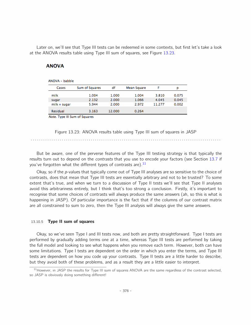
Later on, we’ll see that Type III tests can be redeemed in some contexts, but first let’s take a lookat the ANOVA results table using Type III sum of squares, see Figure 13.23.

Figure 13.23: ANOVA results table using Type III sum of squares in JASP

. . . . . . . . . . . . . . . . . . . . . . . . . . . . . . . . . . . . . . . . . . . . . . . . . . . . . . . . . . . . . . . . . . . . . . . . . . . . . . . . . . . . . . . . . . . .

But be aware, one of the perverse features of the Type III testing strategy is that typically theresults turn out to depend on the contrasts that you use to encode your factors (see Section 13.7 ifyou’ve forgotten what the different types of contrasts are).11

Okay, so if the p-values that typically come out of Type III analyses are so sensitive to the choice ofcontrasts, does that mean that Type III tests are essentially arbitrary and not to be trusted? To someextent that’s true, and when we turn to a discussion of Type II tests we’ll see that Type II analysesavoid this arbitrariness entirely, but I think that’s too strong a conclusion. Firstly, it’s important torecognise that some choices of contrasts will always produce the same answers (ah, so this is what ishappening in JASP). Of particular importance is the fact that if the columns of our contrast matrixare all constrained to sum to zero, then the Type III analysis will always give the same answers.

13.10.5 Type II sum of squares

Okay, so we’ve seen Type I and III tests now, and both are pretty straightforward. Type I tests areperformed by gradually adding terms one at a time, whereas Type III tests are performed by takingthe full model and looking to see what happens when you remove each term. However, both can havesome limitations. Type I tests are dependent on the order in which you enter the terms, and Type IIItests are dependent on how you code up your contrasts. Type II tests are a little harder to describe,but they avoid both of these problems, and as a result they are a little easier to interpret.

11However, in JASP the results for Type III sum of squares ANOVA are the same regardless of the contrast selected,so JASP is obviously doing something different!

- 376 -

Type II tests are broadly similar to Type III tests. Start with a “full” model, and test a particularterm by deleting it from that model. However, Type II tests are based on the marginality principlewhich states that you should not omit a lower order term from your model if there are any higherorder ones that depend on it. So, for instance, if your model contains the two-way interaction A*B (a2nd order term), then it really ought to contain the main effects A and B (1st order terms). Similarly,if it contains a three-way interaction term A*B*C, then the model must also include the main effectsA, B and C as well as the simpler interactions A*B, A*C and B*C. Type III tests routinely violate themarginality principle. For instance, consider the test of the main effect of A in the context of athree-way ANOVA that includes all possible interaction terms. According to Type III tests, our nulland alternative models are:

Null model: outcome ~ B + C + A*B + A*C + B*C + A*B*CAlternative model: outcome ~ A + B + C + A*B + A*C + B*C + A*B*C

Notice that the null hypothesis omits A, but includes A*B, A*C and A*B*C as part of the model.This, according to the Type II tests, is not a good choice of null hypothesis. What we should doinstead, if we want to test the null hypothesis that A is not relevant to our outcome, is to specify thenull hypothesis that is the most complicated model that does not rely on A in any form, even as aninteraction. The alternative hypothesis corresponds to this null model plus a main effect term of A.This is a lot closer to what most people would intuitively think of as a “main effect of A”, and it yieldsthe following as our Type II test of the main effect of A:12

Null model: outcome ~ B + C + B*CAlternative model: outcome ~ A + B + C + B*C

Anyway, just to give you a sense of how the Type II tests play out, here’s the full table of tests thatwould be applied in a three-way factorial ANOVA:

Term beingtested is

Null model is outcome ~ ... Alternative model is outcome ~ ...

A B + C + B*C A + B + C + B*CB A + C + A*C A + B + C + A*CC A + B + A*B A + B + C + A*BA*B A + B + C + A*C + B*C A + B + C + A*B + A*C + B*CA*C A + B + C + A*B + B*C A + B + C + A*B + A*C + B*CB*C A + B + C + A*B + A*C A + B + C + A*B + A*C + B*CA*B*C A + B + C + A*B + A*C + B*C A + B + C + A*B + A*C + B*C + A*B*C

In the context of the two way ANOVA that we’ve been using in the coffee data, the hypothesis tests12Note, of course, that this does depend on the model that the user specified. If the original ANOVA model doesn’t

contain an interaction term for B*C, then obviously it won’t appear in either the null or the alternative. But that’s truefor Types I, II and III. They never include any terms that you didn’t include, but they make different choices about howto construct tests for the ones that you did include.

- 377 -

are even simpler. The main effect of sugar corresponds to an F -test comparing these two models:

Null model: babble ~ milkAlternative model: babble ~ sugar + milk

The test for the main effect of milk is

Null model: babble ~ sugarAlternative model: babble ~ sugar + milk

Finally, the test for the interaction sugar*milk is:


Running the tests are again straightforward. Just select ‘Type 2’ in the ‘Sum of squares’ selectionbox in the JASP ‘ANOVA’ - ‘Model’ options, This gives us the ANOVA table shown in Figure 13.24.

Figure 13.24: ANOVA results table using Type II sum of squares in JASP

. . . . . . . . . . . . . . . . . . . . . . . . . . . . . . . . . . . . . . . . . . . . . . . . . . . . . . . . . . . . . . . . . . . . . . . . . . . . . . . . . . . . . . . . . . . .

Type II tests have some clear advantages over Type I and Type III tests. They don’t depend onthe order in which you specify factors (unlike Type I), and they don’t depend on the contrasts thatyou use to specify your factors (unlike Type III). And although opinions may differ on this last point,and it will definitely depend on what you’re trying to do with your data, I do think that the hypothesistests that they specify are more likely to correspond to something that you actually care about. Asa consequence, I find that it’s usually easier to interpret the results of a Type II test than the resultsof a Type I or Type III test. For this reason my tentative advice is that, if you can’t think of anyobvious model comparisons that directly map onto your research questions but you still want to runan ANOVA in an unbalanced design, Type II tests are probably a better choice than Type I or Type

- 378 -

III.13

13.10.6 Effect sizes (and non-additive sums of squares)

JASP also provides the effect sizes η2 and partial η2 when you select these options. However,when you’ve got an unbalanced design there’s a bit of extra complexity involved.

If you remember back to our very early discussions of ANOVA, one of the key ideas behind thesums of squares calculations is that if we add up all the SS terms associated with the effects in themodel, and add that to the residual SS, they’re supposed to add up to the total sum of squares. And,on top of that, the whole idea behind η2 is that, because you’re dividing one of the SS terms bythe total SS value, an η2 value can be interpreted as the proportion of variance accounted for by aparticular term. But this is not so straightforward in unbalanced designs because some of the variancegoes “missing”.

This seems a bit odd at first, but here’s why. When you have unbalanced designs your factorsbecome correlated with one another, and it becomes difficult to tell the difference between the effectof Factor A and the effect of Factor B. In the extreme case, suppose that we’d run a 2ˆ 2 design inwhich the number of participants in each group had been as follows:

sugar no sugarmilk 100 0no milk 0 100

Here we have a spectacularly unbalanced design: 100 people have milk and sugar, 100 people haveno milk and no sugar, and that’s all. There are 0 people with milk and no sugar, and 0 people withsugar but no milk. Now suppose that, when we collected the data, it turned out there is a large (andstatistically significant) difference between the “milk and sugar” group and the “no-milk and no-sugar”group. Is this a main effect of sugar? A main effect of milk? Or an interaction? It’s impossible totell, because the presence of sugar has a perfect association with the presence of milk. Now supposethe design had been a little more balanced:

sugar no sugarmilk 100 5no milk 5 100

13I find it amusing to note that the default in R is Type I and the default in SPSS, JASP, and jamovi is Type III. Neitherof these appeals to me all that much. Relatedly, I find it depressing that almost nobody in the psychological literatureever bothers to report which Type of tests they ran, much less the order of variables (for Type I) or the contrasts used(for Type III). Often they don’t report what software they used either. The only way I can ever make any sense of whatpeople typically report is to try to guess from auxiliary cues which software they were using, and to assume that theynever changed the default settings. Please don’t do this! Now that you know about these issues make sure you indicatewhat software you used, and if you’re reporting ANOVA results for unbalanced data, then specify what Type of tests youran, specify order information if you’ve done Type I tests and specify contrasts if you’ve done Type III tests. Or, evenbetter, do hypotheses tests that correspond to things you really care about and then report those!

- 379 -

This time around, it’s technically possible to distinguish between the effect of milk and the effect ofsugar, because we have a few people that have one but not the other. However, it will still be prettydifficult to do so, because the association between sugar and milk is still extremely strong, and thereare so few observations in two of the groups. Again, we’re very likely to be in the situation wherewe know that the predictor variables (milk and sugar) are related to the outcome (babbling), but wedon’t know if the nature of that relationship is a main effect of one or the other predictor, or theinteraction.

This uncertainty is the reason for the missing variance. The “missing” variance corresponds tovariation in the outcome variable that is clearly attributable to the predictors, but we don’t knowwhich of the effects in the model is responsible. When you calculate Type I sum of squares, novariance ever goes missing. The sequential nature of Type I sum of squares means that the ANOVAautomatically attributes this variance to whichever effects are entered first. However, the Type II andType III tests are more conservative. Variance that cannot be clearly attributed to a specific effectdoesn’t get attributed to any of them, and it goes missing.

13.11

Summary

• Factorial ANOVA with balanced designs, without interactions (Section 13.1) and with interac-tions included (Section 13.2)

• Effect size, estimated means, and confidence intervals in a factorial ANOVA (Section 13.3)

• Checking assumptions in ANOVA (Section 13.4)

• Analysis of Covariance (ANCOVA) (Section 13.5)

• Understanding the linear model underlying ANOVA, including different contrasts (Section 13.6and 13.7)

• Post hoc testing using Tukey’s HSD (Section 13.8) and a brief commentary on planned com-parisons (Section 13.9)

• Factorial ANOVA with unbalanced designs (Section 13.10)

- 380 -

Part V.

Endings, alternatives and prospects

- 381 -

14. Bayesian statistics

In our reasonings concerning matter of fact, there are all imaginable degrees of assurance,from the highest certainty to the lowest species of moral evidence. A wise man, therefore,proportions his belief to the evidence.

– David Hume1

The ideas I’ve presented to you in this book describe inferential statistics from the frequentistperspective. I’m not alone in doing this. In fact, almost every textbook given to undergraduatepsychology students presents the opinions of the frequentist statistician as the theory of inferentialstatistics, the one true way to do things. I have taught this way for practical reasons. The frequentistview of statistics dominated the academic field of statistics for most of the 20th century, and thisdominance is even more extreme among applied scientists. It was and is current practice amongpsychologists to use frequentist methods. Because frequentist methods are ubiquitous in scientificpapers, every student of statistics needs to understand those methods, otherwise they will be unableto make sense of what those papers are saying! Unfortunately, in my opinion at least, the currentpractice in psychology is often misguided and the reliance on frequentist methods is partly to blame. Inthis chapter I explain why I think this and provide an introduction to Bayesian statistics, an approachthat I think is generally superior to the orthodox approach.

This chapter comes in two parts. In Sections 14.1 through 14.3 I talk about what Bayesian statisticsare all about, covering the basic mathematical rules for how it works as well as an explanation for whyI think the Bayesian approach is so useful. Afterwards, I provide a brief overview of how you can doBayesian versions of t-tests (Section 14.4).

1http://en.wikiquote.org/wiki/David_Hume.

- 383 -

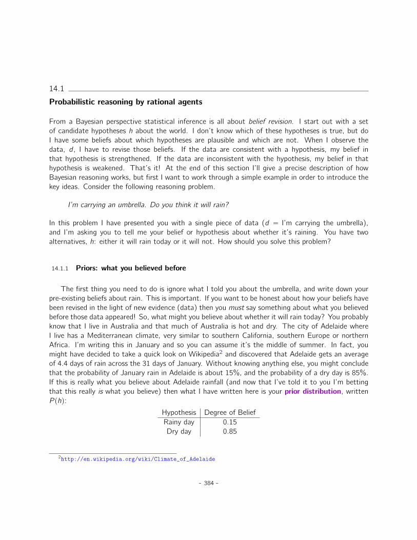
http://en.wikiquote.org/wiki/David_Hume

14.1

Probabilistic reasoning by rational agents

From a Bayesian perspective statistical inference is all about belief revision. I start out with a setof candidate hypotheses h about the world. I don’t know which of these hypotheses is true, but doI have some beliefs about which hypotheses are plausible and which are not. When I observe thedata, d , I have to revise those beliefs. If the data are consistent with a hypothesis, my belief inthat hypothesis is strengthened. If the data are inconsistent with the hypothesis, my belief in thathypothesis is weakened. That’s it! At the end of this section I’ll give a precise description of howBayesian reasoning works, but first I want to work through a simple example in order to introduce thekey ideas. Consider the following reasoning problem.

I’m carrying an umbrella. Do you think it will rain?

In this problem I have presented you with a single piece of data (d “ I’m carrying the umbrella),and I’m asking you to tell me your belief or hypothesis about whether it’s raining. You have twoalternatives, h: either it will rain today or it will not. How should you solve this problem?

14.1.1 Priors: what you believed before

The first thing you need to do is ignore what I told you about the umbrella, and write down yourpre-existing beliefs about rain. This is important. If you want to be honest about how your beliefs havebeen revised in the light of new evidence (data) then you must say something about what you believedbefore those data appeared! So, what might you believe about whether it will rain today? You probablyknow that I live in Australia and that much of Australia is hot and dry. The city of Adelaide whereI live has a Mediterranean climate, very similar to southern California, southern Europe or northernAfrica. I’m writing this in January and so you can assume it’s the middle of summer. In fact, youmight have decided to take a quick look on Wikipedia2 and discovered that Adelaide gets an averageof 4.4 days of rain across the 31 days of January. Without knowing anything else, you might concludethat the probability of January rain in Adelaide is about 15%, and the probability of a dry day is 85%.If this is really what you believe about Adelaide rainfall (and now that I’ve told it to you I’m bettingthat this really is what you believe) then what I have written here is your prior distribution, writtenP phq:

Hypothesis Degree of BeliefRainy day 0.15Dry day 0.85

2http://en.wikipedia.org/wiki/Climate_of_Adelaide

- 384 -

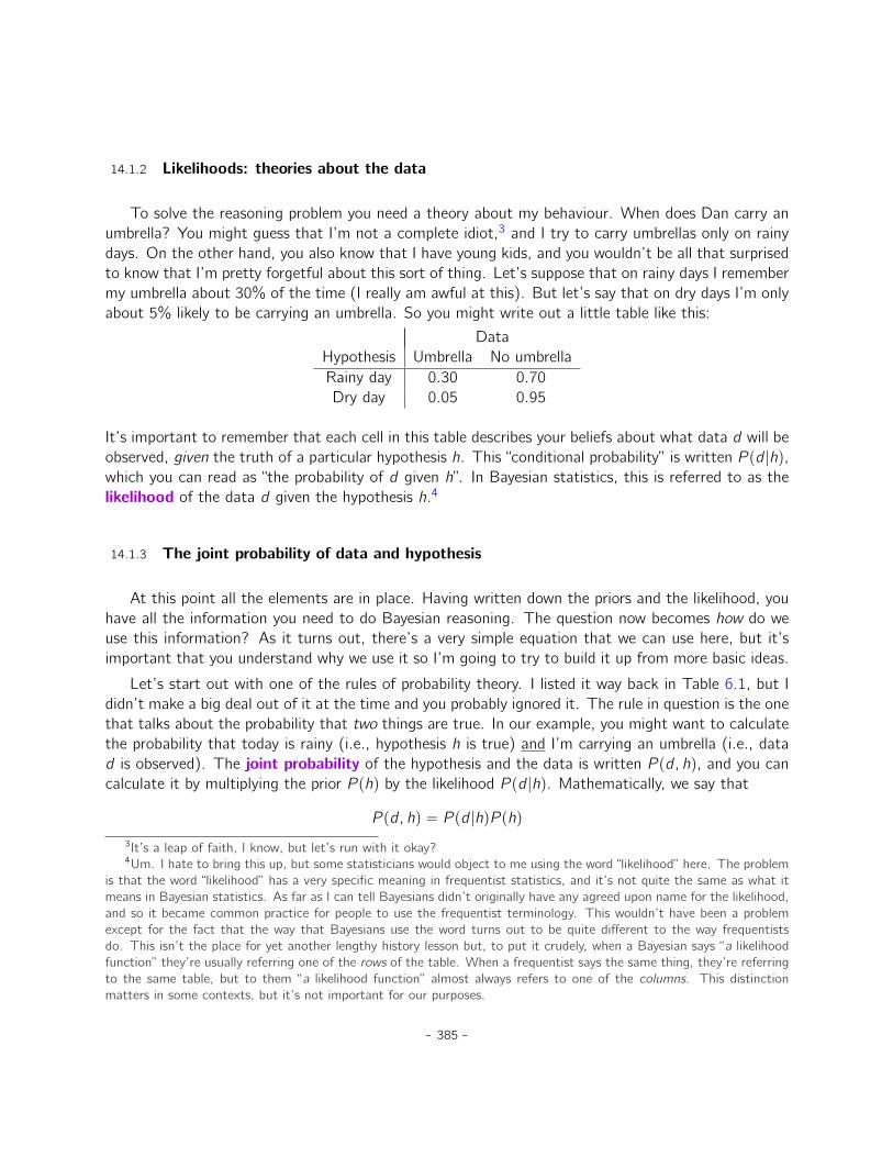
http://en.wikipedia.org/wiki/Climate_of_Adelaide

14.1.2 Likelihoods: theories about the data

To solve the reasoning problem you need a theory about my behaviour. When does Dan carry anumbrella? You might guess that I’m not a complete idiot,3 and I try to carry umbrellas only on rainydays. On the other hand, you also know that I have young kids, and you wouldn’t be all that surprisedto know that I’m pretty forgetful about this sort of thing. Let’s suppose that on rainy days I remembermy umbrella about 30% of the time (I really am awful at this). But let’s say that on dry days I’m onlyabout 5% likely to be carrying an umbrella. So you might write out a little table like this:

DataHypothesis Umbrella No umbrellaRainy day 0.30 0.70Dry day 0.05 0.95

It’s important to remember that each cell in this table describes your beliefs about what data d will beobserved, given the truth of a particular hypothesis h. This “conditional probability” is written P pd |hq,which you can read as “the probability of d given h”. In Bayesian statistics, this is referred to as thelikelihood of the data d given the hypothesis h.4

14.1.3 The joint probability of data and hypothesis

At this point all the elements are in place. Having written down the priors and the likelihood, youhave all the information you need to do Bayesian reasoning. The question now becomes how do weuse this information? As it turns out, there’s a very simple equation that we can use here, but it’simportant that you understand why we use it so I’m going to try to build it up from more basic ideas.

Let’s start out with one of the rules of probability theory. I listed it way back in Table 6.1, but Ididn’t make a big deal out of it at the time and you probably ignored it. The rule in question is the onethat talks about the probability that two things are true. In our example, you might want to calculatethe probability that today is rainy (i.e., hypothesis h is true) and I’m carrying an umbrella (i.e., datad is observed). The joint probability of the hypothesis and the data is written P pd, hq, and you cancalculate it by multiplying the prior P phq by the likelihood P pd |hq. Mathematically, we say that

P pd, hq “ P pd |hqP phq

3It’s a leap of faith, I know, but let’s run with it okay?4Um. I hate to bring this up, but some statisticians would object to me using the word “likelihood” here. The problem

is that the word “likelihood” has a very specific meaning in frequentist statistics, and it’s not quite the same as what itmeans in Bayesian statistics. As far as I can tell Bayesians didn’t originally have any agreed upon name for the likelihood,and so it became common practice for people to use the frequentist terminology. This wouldn’t have been a problemexcept for the fact that the way that Bayesians use the word turns out to be quite different to the way frequentistsdo. This isn’t the place for yet another lengthy history lesson but, to put it crudely, when a Bayesian says “a likelihoodfunction” they’re usually referring one of the rows of the table. When a frequentist says the same thing, they’re referringto the same table, but to them “a likelihood function” almost always refers to one of the columns. This distinctionmatters in some contexts, but it’s not important for our purposes.

- 385 -

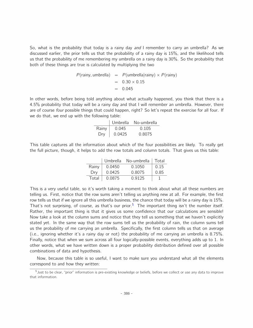
So, what is the probability that today is a rainy day and I remember to carry an umbrella? As wediscussed earlier, the prior tells us that the probability of a rainy day is 15%, and the likelihood tellsus that the probability of me remembering my umbrella on a rainy day is 30%. So the probability thatboth of these things are true is calculated by multiplying the two

P prainy, umbrellaq “ P pumbrella|rainyq ˆ P prainyq

“ 0.30ˆ 0.15

“ 0.045

In other words, before being told anything about what actually happened, you think that there is a4.5% probability that today will be a rainy day and that I will remember an umbrella. However, thereare of course four possible things that could happen, right? So let’s repeat the exercise for all four. Ifwe do that, we end up with the following table:

Umbrella No-umbrellaRainy 0.045 0.105Dry 0.0425 0.8075

This table captures all the information about which of the four possibilities are likely. To really getthe full picture, though, it helps to add the row totals and column totals. That gives us this table:

Umbrella No-umbrella TotalRainy 0.0450 0.1050 0.15Dry 0.0425 0.8075 0.85Total 0.0875 0.9125 1

This is a very useful table, so it’s worth taking a moment to think about what all these numbers aretelling us. First, notice that the row sums aren’t telling us anything new at all. For example, the firstrow tells us that if we ignore all this umbrella business, the chance that today will be a rainy day is 15%.That’s not surprising, of course, as that’s our prior.5 The important thing isn’t the number itself.Rather, the important thing is that it gives us some confidence that our calculations are sensible!Now take a look at the column sums and notice that they tell us something that we haven’t explicitlystated yet. In the same way that the row sums tell us the probability of rain, the column sums tellus the probability of me carrying an umbrella. Specifically, the first column tells us that on average(i.e., ignoring whether it’s a rainy day or not) the probability of me carrying an umbrella is 8.75%.Finally, notice that when we sum across all four logically-possible events, everything adds up to 1. Inother words, what we have written down is a proper probability distribution defined over all possiblecombinations of data and hypothesis.

Now, because this table is so useful, I want to make sure you understand what all the elementscorrespond to and how they written:

5Just to be clear, “prior” information is pre-existing knowledge or beliefs, before we collect or use any data to improvethat information.

- 386 -

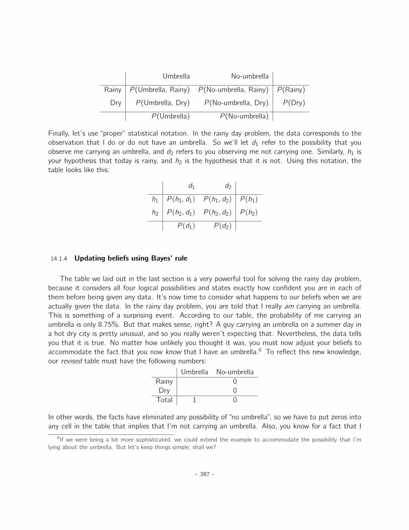
Umbrella No-umbrella

Rainy P (Umbrella, Rainy) P (No-umbrella, Rainy) P (Rainy)

Dry P (Umbrella, Dry) P (No-umbrella, Dry) P (Dry)

P (Umbrella) P (No-umbrella)

Finally, let’s use “proper” statistical notation. In the rainy day problem, the data corresponds to theobservation that I do or do not have an umbrella. So we’ll let d1 refer to the possibility that youobserve me carrying an umbrella, and d2 refers to you observing me not carrying one. Similarly, h1 isyour hypothesis that today is rainy, and h2 is the hypothesis that it is not. Using this notation, thetable looks like this:

d1 d2

h1 P ph1, d1q P ph1, d2q P ph1q

h2 P ph2, d1q P ph2, d2q P ph2q

P pd1q P pd2q

14.1.4 Updating beliefs using Bayes’ rule

The table we laid out in the last section is a very powerful tool for solving the rainy day problem,because it considers all four logical possibilities and states exactly how confident you are in each ofthem before being given any data. It’s now time to consider what happens to our beliefs when we areactually given the data. In the rainy day problem, you are told that I really am carrying an umbrella.This is something of a surprising event. According to our table, the probability of me carrying anumbrella is only 8.75%. But that makes sense, right? A guy carrying an umbrella on a summer day ina hot dry city is pretty unusual, and so you really weren’t expecting that. Nevertheless, the data tellsyou that it is true. No matter how unlikely you thought it was, you must now adjust your beliefs toaccommodate the fact that you now know that I have an umbrella.6 To reflect this new knowledge,our revised table must have the following numbers:

Umbrella No-umbrellaRainy 0Dry 0Total 1 0

In other words, the facts have eliminated any possibility of “no umbrella”, so we have to put zeros intoany cell in the table that implies that I’m not carrying an umbrella. Also, you know for a fact that I

6If we were being a bit more sophisticated, we could extend the example to accommodate the possibility that I’mlying about the umbrella. But let’s keep things simple, shall we?

- 387 -

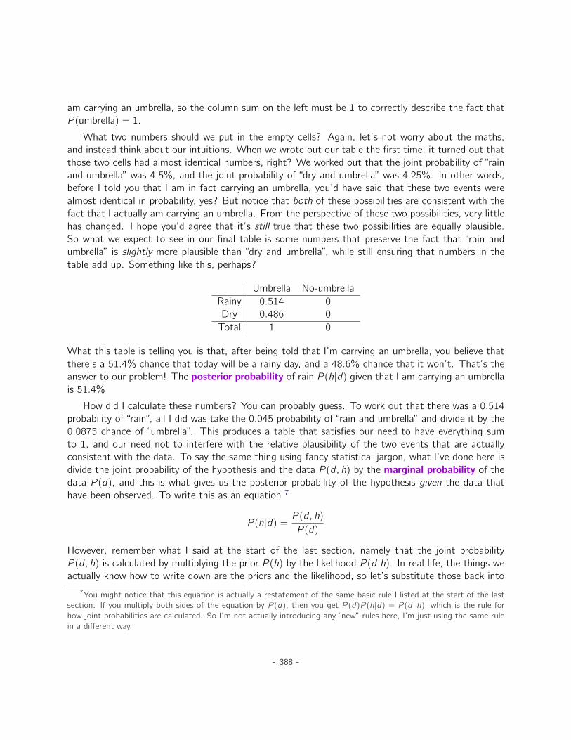
am carrying an umbrella, so the column sum on the left must be 1 to correctly describe the fact thatP pumbrellaq “ 1.

What two numbers should we put in the empty cells? Again, let’s not worry about the maths,and instead think about our intuitions. When we wrote out our table the first time, it turned out thatthose two cells had almost identical numbers, right? We worked out that the joint probability of “rainand umbrella” was 4.5%, and the joint probability of “dry and umbrella” was 4.25%. In other words,before I told you that I am in fact carrying an umbrella, you’d have said that these two events werealmost identical in probability, yes? But notice that both of these possibilities are consistent with thefact that I actually am carrying an umbrella. From the perspective of these two possibilities, very littlehas changed. I hope you’d agree that it’s still true that these two possibilities are equally plausible.So what we expect to see in our final table is some numbers that preserve the fact that “rain andumbrella” is slightly more plausible than “dry and umbrella”, while still ensuring that numbers in thetable add up. Something like this, perhaps?

Umbrella No-umbrellaRainy 0.514 0Dry 0.486 0Total 1 0

What this table is telling you is that, after being told that I’m carrying an umbrella, you believe thatthere’s a 51.4% chance that today will be a rainy day, and a 48.6% chance that it won’t. That’s theanswer to our problem! The posterior probability of rain P ph|dq given that I am carrying an umbrellais 51.4%

How did I calculate these numbers? You can probably guess. To work out that there was a 0.514probability of “rain”, all I did was take the 0.045 probability of “rain and umbrella” and divide it by the0.0875 chance of “umbrella”. This produces a table that satisfies our need to have everything sumto 1, and our need not to interfere with the relative plausibility of the two events that are actuallyconsistent with the data. To say the same thing using fancy statistical jargon, what I’ve done here isdivide the joint probability of the hypothesis and the data P pd, hq by the marginal probability of thedata P pdq, and this is what gives us the posterior probability of the hypothesis given the data thathave been observed. To write this as an equation 7

P ph|dq “P pd, hq

P pdq

However, remember what I said at the start of the last section, namely that the joint probabilityP pd, hq is calculated by multiplying the prior P phq by the likelihood P pd |hq. In real life, the things weactually know how to write down are the priors and the likelihood, so let’s substitute those back into

7You might notice that this equation is actually a restatement of the same basic rule I listed at the start of the lastsection. If you multiply both sides of the equation by P pdq, then you get P pdqP ph|dq “ P pd, hq, which is the rule forhow joint probabilities are calculated. So I’m not actually introducing any “new” rules here, I’m just using the same rulein a different way.

- 388 -

the equation. This gives us the following formula for the posterior probability

P ph|dq “P pd |hqP phq

P pdq

And this formula, folks, is known as Bayes’ rule. It describes how a learner starts out with prior beliefsabout the plausibility of different hypotheses, and tells you how those beliefs should be revised in theface of data. In the Bayesian paradigm, all statistical inference flows from this one simple rule.

14.2

Bayesian hypothesis tests

In Chapter 8 I described the orthodox approach to hypothesis testing. It took an entire chapter todescribe, because null hypothesis testing is a very elaborate contraption that people find very hard tomake sense of. In contrast, the Bayesian approach to hypothesis testing is incredibly simple. Let’s picka setting that is closely analogous to the orthodox scenario. There are two hypotheses that we wantto compare, a null hypothesis h0 and an alternative hypothesis h1. Prior to running the experimentwe have some beliefs P phq about which hypotheses are true. We run an experiment and obtain datad . Unlike frequentist statistics, Bayesian statistics does allow us to talk about the probability thatthe null hypothesis is true. Better yet, it allows us to calculate the posterior probability of the nullhypothesis, using Bayes’ rule

P ph0|dq “P pd |h0qP ph0q

P pdq

This formula tells us exactly how much belief we should have in the null hypothesis after havingobserved the data d . Similarly, we can work out how much belief to place in the alternative hypothesisusing essentially the same equation. All we do is change the subscript

P ph1|dq “P pd |h1qP ph1q

P pdq

It’s all so simple that I feel like an idiot even bothering to write these equations down, since all I’mdoing is copying Bayes rule from the previous section.8

14.2.1 The Bayes factor

In practice, most Bayesian data analysts tend not to talk in terms of the raw posterior probabilitiesP ph0|dq and P ph1|dq. Instead, we tend to talk in terms of the posterior odds ratio. Think of it

8Obviously, this is a highly simplified story. All the complexity of real life Bayesian hypothesis testing comes downto how you calculate the likelihood P pd |hq when the hypothesis h is a complex and vague thing. I’m not going to talkabout those complexities in this book, but I do want to highlight that although this simple story is true as far as it goes,real life is messier than I’m able to cover in an introductory stats textbook.

- 389 -

like betting. Suppose, for instance, the posterior probability of the null hypothesis is 25%, and theposterior probability of the alternative is 75%. The alternative hypothesis is three times as probableas the null, so we say that the odds are 3:1 in favour of the alternative. Mathematically, all we haveto do to calculate the posterior odds is divide one posterior probability by the other

P ph1|dq

P ph0|dq“

0.75

0.25“ 3

Or, to write the same thing in terms of the equations above

P ph1|dq

P ph0|dq“P pd |h1q

P pd |h0qˆP ph1q

P ph0q

Actually, this equation is worth expanding on. There are three different terms here that you shouldknow. On the left hand side, we have the posterior odds, which tells you what you believe about therelative plausibilty of the null hypothesis and the alternative hypothesis after seeing the data. On theright hand side, we have the prior odds, which indicates what you thought before seeing the data. Inthe middle, we have the Bayes factor, which describes the amount of evidence provided by the data

P ph1|dq

P ph0|dq“

P pd |h1q

P pd |h0qˆ

P ph1q

P ph0q

Ò Ò Ò

Posterior odds Bayes factor Prior odds

The Bayes factor (sometimes abbreviated as BF) has a special place in Bayesian hypothesis testing,because it serves a similar role to the p-value in orthodox hypothesis testing. The Bayes factorquantifies the strength of evidence provided by the data, and as such it is the Bayes factor that peopletend to report when running a Bayesian hypothesis test. The reason for reporting Bayes factors ratherthan posterior odds is that different researchers will have different priors. Some people might have astrong bias to believe the null hypothesis is true, others might have a strong bias to believe it is false.Because of this, the polite thing for an applied researcher to do is report the Bayes factor. That way,anyone reading the paper can multiply the Bayes factor by their own personal prior odds, and theycan work out for themselves what the posterior odds would be. In any case, by convention we like topretend that we give equal consideration to both the null hypothesis and the alternative, in which casethe prior odds equals 1, and the posterior odds becomes the same as the Bayes factor.

14.2.2 Interpreting Bayes factors

One of the really nice things about the Bayes factor is the numbers are inherently meaningful. If yourun an experiment and you compute a Bayes factor of 4, it means that the evidence provided by yourdata corresponds to betting odds of 4:1 in favour of the alternative. However, there have been someattempts to quantify the standards of evidence that would be considered meaningful in a scientificcontext. The two most widely used are from Jeffreys (1961) and Kass and Raftery (1995). Of thetwo, I tend to prefer the Kass et al. (1995) table because it’s a bit more conservative. So here it is:

- 390 -

Bayes factor Interpretation1 - 3 Negligible evidence3 - 20 Positive evidence

20 - 150 Strong evidenceą150 Very strong evidence

And to be perfectly honest, I think that even the Kass et al. (1995) standards are being a bit charitable.If it were up to me, I’d have called the “positive evidence” category “weak evidence”. To me, anythingin the range 3:1 to 20:1 is “weak” or “modest” evidence at best. But there are no hard and fast ruleshere. What counts as strong or weak evidence depends entirely on how conservative you are and uponthe standards that your community insists upon before it is willing to label a finding as “true”.

In any case, note that all the numbers listed above make sense if the Bayes factor is greater than1 (i.e., the evidence favours the alternative hypothesis). However, one big practical advantage of theBayesian approach relative to the orthodox approach is that it also allows you to quantify evidence forthe null. When that happens, the Bayes factor will be less than 1. You can choose to report a Bayesfactor less than 1, but to be honest I find it confusing. For example, suppose that the likelihood ofthe data under the null hypothesis P pd |h0q is equal to 0.2, and the corresponding likelihood P pd |h1q

under the alternative hypothesis is 0.1. Using the equations given above, Bayes factor here would be

BF “P pd |h1q

P pd |h0q“

0.1

0.2“ 0.5

Read literally, this result tells is that the evidence in favour of the alternative is 0.5 to 1. I find thishard to understand. To me, it makes a lot more sense to turn the equation “upside down”, and reportthe amount op evidence in favour of the null. In other words, what we calculate is this

BF1 “P pd |h0q

P pd |h1q“

0.2

0.1“ 2

And what we would report is a Bayes factor of 2:1 in favour of the null. Much easier to understand,and you can interpret this using the table above.

14.3

Why be a Bayesian?

Up to this point I’ve focused exclusively on the logic underpinning Bayesian statistics. We’ve talkedabout the idea of “probability as a degree of belief”, and what it implies about how a rational agentshould reason about the world. The question that you have to answer for yourself is this: how doyou want to do your statistics? Do you want to be an orthodox statistician, relying on samplingdistributions and p-values to guide your decisions? Or do you want to be a Bayesian, relying on thingslike prior beliefs, Bayes factors and the rules for rational belief revision? And to be perfectly honest, Ican’t answer this question for you. Ultimately it depends on what you think is right. It’s your call andyour call alone. That being said, I can talk a little about why I prefer the Bayesian approach.

- 391 -

14.3.1 Statistics that mean what you think they mean

You keep using that word. I do not think it means what you think it means

– Inigo Montoya, The Princess Bride9

To me, one of the biggest advantages to the Bayesian approach is that it answers the rightquestions. Within the Bayesian framework, it is perfectly sensible and allowable to refer to “theprobability that a hypothesis is true”. You can even try to calculate this probability. Ultimately, isn’tthat what you want your statistical tests to tell you? To an actual human being, this would seem tobe the whole point of doing statistics, i.e., to determine what is true and what isn’t. Any time thatyou aren’t exactly sure about what the truth is, you should use the language of probability theory tosay things like “there is an 80% chance that Theory A is true, but a 20% chance that Theory B istrue instead”.

This seems so obvious to a human, yet it is explicitly forbidden within the orthodox framework. Toa frequentist, such statements are a nonsense because “the theory is true” is not a repeatable event.A theory is true or it is not, and no probabilistic statements are allowed, no matter how much youmight want to make them. There’s a reason why, back in Section 8.5, I repeatedly warned you not tointerpret the p-value as the probability that the null hypothesis is true. There’s a reason why almostevery textbook on statstics is forced to repeat that warning. It’s because people desperately wantthat to be the correct interpretation. Frequentist dogma notwithstanding, a lifetime of experience ofteaching undergraduates and of doing data analysis on a daily basis suggests to me that most actualhumans think that “the probability that the hypothesis is true” is not only meaningful, it’s the thingwe care most about. It’s such an appealing idea that even trained statisticians fall prey to the mistakeof trying to interpret a p-value this way. For example, here is a quote from an official Newspoll reportin 2013, explaining how to interpret their (frequentist) data analysis:10

Throughout the report, where relevant, statistically significant changes have been noted.All significance tests have been based on the 95 percent level of confidence. This meansthat if a change is noted as being statistically significant, there is a 95 percentprobability that a real change has occurred, and is not simply due to chance variation.(emphasis added)

Nope! That’s not what p ă .05 means. That’s not what 95% confidence means to a frequentiststatistician. The bolded section is just plain wrong. Orthodox methods cannot tell you that “there is a95% chance that a real change has occurred”, because this is not the kind of event to which frequentistprobabilities may be assigned. To an ideological frequentist, this sentence should be meaningless. Even

9http://www.imdb.com/title/tt0093779/quotes. I should note in passing that I’m not the first person to use thisquote to complain about frequentist methods. Rich Morey and colleagues had the idea first. I’m shamelessly stealingit because it’s such an awesome pull quote to use in this context and I refuse to miss any opportunity to quote ThePrincess Bride.

10http://about.abc.net.au/reports-publications/appreciation-survey-summary-report-2013/

- 392 -

http://www.imdb.com/title/tt0093779/quotes

http://about.abc.net.au/reports-publications/appreciation-survey-summary-report-2013/

if you’re a more pragmatic frequentist, it’s still the wrong definition of a p-value. It is simply not anallowed or correct thing to say if you want to rely on orthodox statistical tools.

On the other hand, let’s suppose you are a Bayesian. Although the bolded passage is the wrongdefinition of a p-value, it’s pretty much exactly what a Bayesian means when they say that the posteriorprobability of the alternative hypothesis is greater than 95%. And here’s the thing. If the Bayesianposterior is actually the thing you want to report, why are you even trying to use orthodox methods?If you want to make Bayesian claims, all you have to do is be a Bayesian and use Bayesian tools.

Speaking for myself, I found this to be the most liberating thing about switching to the Bayesianview. Once you’ve made the jump, you no longer have to wrap your head around counter-intuitivedefinitions of p-values. You don’t have to bother remembering why you can’t say that you’re 95%confident that the true mean lies within some interval. All you have to do is be honest about whatyou believed before you ran the study and then report what you learned from doing it. Sounds nice,doesn’t it? To me, this is the big promise of the Bayesian approach. You do the analysis you reallywant to do, and express what you really believe the data are telling you.

14.3.2 Evidentiary standards you can believe

If [p] is below .02 it is strongly indicated that the [null] hypothesis fails to account for thewhole of the facts. We shall not often be astray if we draw a conventional line at .05 andconsider that [smaller values of p] indicate a real discrepancy.

– Sir Ronald Fisher (1925)

Consider the quote above by Sir Ronald Fisher, one of the founders of what has become theorthodox approach to statistics. If anyone has ever been entitled to express an opinion about theintended function of p-values, it’s Fisher. In this passage, taken from his classic guide StatisticalMethods for Research Workers, he’s pretty clear about what it means to reject a null hypothesis atp ă .05. In his opinion, if we take p ă .05 to mean there is “a real effect”, then “we shall not often beastray”. This view is hardly unusual. In my experience, most practitioners express views very similarto Fisher’s. In essence, the p ă .05 convention is assumed to represent a fairly stringent evidentialstandard.

Well, how true is that? One way to approach this question is to try to convert p-values toBayes factors, and see how the two compare. It’s not an easy thing to do because a p-value is afundamentally different kind of calculation to a Bayes factor, and they don’t measure the same thing.However, there have been some attempts to work out the relationship between the two, and it’ssomewhat surprising. For example, Johnson (2013) presents a pretty compelling case that (for t-testsat least) the p ă .05 threshold corresponds roughly to a Bayes factor of somewhere between 3:1 and5:1 in favour of the alternative. If that’s right, then Fisher’s claim is a bit of a stretch. Let’s supposethat the null hypothesis is true about half the time (i.e., the prior probability of H0 is 0.5), and weuse those numbers to work out the posterior probability of the null hypothesis given that it has beenrejected at p ă .05. Using the data from Johnson (2013), we see that if you reject the null at p ă .05,

- 393 -

you’ll be correct about 80% of the time. I don’t know about you but, in my opinion, an evidentialstandard that ensures you’ll be wrong on 20% of your decisions isn’t good enough. The fact remainsthat, quite contrary to Fisher’s claim, if you reject at p ă .05 you shall quite often go astray. It’s nota very stringent evidential threshold at all.

14.3.3 The p-value is a lie.

The cake is a lie.The cake is a lie.The cake is a lie.The cake is a lie.

– Portal11

Okay, at this point you might be thinking that the real problem is not with orthodox statistics,just the p ă .05 standard. In one sense, that’s true. The recommendation that Johnson (2013) givesis not that “everyone must be a Bayesian now”. Instead, the suggestion is that it would be wiser toshift the conventional standard to something like a p ă .01 level. That’s not an unreasonable viewto take, but in my view the problem is a little more severe than that. In my opinion, there’s a fairlybig problem built into the way most (but not all) orthodox hypothesis tests are constructed. They aregrossly naive about how humans actually do research, and because of this most p-values are wrong.

Sounds like an absurd claim, right? Well, consider the following scenario. You’ve come up with areally exciting research hypothesis and you design a study to test it. You’re very diligent, so you runa power analysis to work out what your sample size should be, and you run the study. You run yourhypothesis test and out pops a p-value of 0.072. Really bloody annoying, right?

What should you do? Here are some possibilities:

1. You conclude that there is no effect and try to publish it as a null result2. You guess that there might be an effect and try to publish it as a “borderline significant” result3. You give up and try a new study4. You collect some more data to see if the p value goes up or (preferably!) drops below the

“magic” criterion of p ă .05

Which would you choose? Before reading any further, I urge you to take some time to think aboutit. Be honest with yourself. But don’t stress about it too much, because you’re screwed no matterwhat you choose. Based on my own experiences as an author, reviewer and editor, as well as storiesI’ve heard from others, here’s what will happen in each case:

• Let’s start with option 1. If you try to publish it as a null result, the paper will struggle to bepublished. Some reviewers will think that p “ .072 is not really a null result. They’ll argue it’s

11http://knowyourmeme.com/memes/the-cake-is-a-lie

- 394 -

http://knowyourmeme.com/memes/the-cake-is-a-lie

borderline significant. Other reviewers will agree it’s a null result but will claim that even thoughsome null results are publishable, yours isn’t. One or two reviewers might even be on your side,but you’ll be fighting an uphill battle to get it through.

• Okay, let’s think about option number 2. Suppose you try to publish it as a borderline significantresult. Some reviewers will claim that it’s a null result and should not be published. Others willclaim that the evidence is ambiguous, and that you should collect more data until you get aclear significant result. Again, the publication process does not favour you.

• Given the difficulties in publishing an “ambiguous” result like p “ .072, option number 3 mightseem tempting: give up and do something else. But that’s a recipe for career suicide. If yougive up and try a new project every time you find yourself faced with ambiguity, your work willnever be published. And if you’re in academia without a publication record you can lose yourjob. So that option is out.

• It looks like you’re stuck with option 4. You don’t have conclusive results, so you decide tocollect some more data and re-run the analysis. Seems sensible, but unfortunately for you, ifyou do this all of your p-values are now incorrect. All of them. Not just the p-values that youcalculated for this study. All of them. All the p-values you calculated in the past and all thep-values you will calculate in the future. Fortunately, no-one will notice. You’ll get published,and you’ll have lied.

Wait, what? How can that last part be true? I mean, it sounds like a perfectly reasonable strategydoesn’t it? You collected some data, the results weren’t conclusive, so now what you want to do iscollect more data until the the results are conclusive. What’s wrong with that?

Honestly, there’s nothing wrong with it. It’s a reasonable, sensible and rational thing to do. In reallife, this is exactly what every researcher does. Unfortunately, the theory of null hypothesis testing asI described it in Chapter 8 forbids you from doing this.12 The reason is that the theory assumes thatthe experiment is finished and all the data are in. And because it assumes the experiment is over,it only considers two possible decisions. If you’re using the conventional p ă .05 threshold, thosedecisions are:

Outcome Actionp less than .05 Reject the nullp greater than .05 Retain the null

12In the interests of being completely honest, I should acknowledge that not all orthodox statistical tests rely on thissilly assumption. There are a number of sequential analysis tools that are sometimes used in clinical trials and the like.These methods are built on the assumption that data are analysed as they arrive, and these tests aren’t horribly brokenin the way I’m complaining about here. However, sequential analysis methods are constructed in a very different fashionto the “standard” version of null hypothesis testing. They don’t make it into any introductory textbooks, and they’re notvery widely used in the psychological literature. The concern I’m raising here is valid for every single orthodox test I’vepresented so far and for almost every test I’ve seen reported in the papers I read.

- 395 -

What you’re doing is adding a third possible action to the decision making problem. Specifically, whatyou’re doing is using the p-value itself as a reason to justify continuing the experiment. And as aconsequence you’ve transformed the decision-making procedure into one that looks more like this:

Outcome Actionp less than .05 Stop the experiment and reject the nullp between .05 and .1 Continue the experimentp greater than .1 Stop the experiment and retain the null

The “basic” theory of null hypothesis testing isn’t built to handle this sort of thing, not in the form Idescribed back in Chapter 8. If you’re the kind of person who would choose to “collect more data” inreal life, it implies that you are not making decisions in accordance with the rules of null hypothesistesting. Even if you happen to arrive at the same decision as the hypothesis test, you aren’t followingthe decision process it implies, and it’s this failure to follow the process that is causing the problem.13

Your p-values are a lie.

Worse yet, they’re a lie in a dangerous way, because they’re all too small. To give you a sense ofjust how bad it can be, consider the following (worst case) scenario. Imagine you’re a really super-enthusiastic researcher on a tight budget who didn’t pay any attention to my warnings above. Youdesign a study comparing two groups. You desperately want to see a significant result at the p ă .05

level, but you really don’t want to collect any more data than you have to (because it’s expensive).In order to cut costs you start collecting data but every time a new observation arrives you run at-test on your data. If the t-tests says p ă .05 then you stop the experiment and report a significantresult. If not, you keep collecting data. You keep doing this until you reach your pre-defined spendinglimit for this experiment. Let’s say that limit kicks in at N “ 1000 observations. As it turns out, thetruth of the matter is that there is no real effect to be found: the null hypothesis is true. So, what’sthe chance that you’ll make it to the end of the experiment and (correctly) conclude that there is noeffect? In an ideal world, the answer here should be 95%. After all, the whole point of the p ă .05

criterion is to control the Type I error rate at 5%, so what we’d hope is that there’s only a 5% chanceof falsely rejecting the null hypothesis in this situation. However, there’s no guarantee that will betrue. You’re breaking the rules. Because you’re running tests repeatedly, “peeking” at your data tosee if you’ve gotten a significant result, all bets are off.

So how bad is it? The answer is shown as the solid black line in Figure 14.1, and it’s astoundinglybad. If you peek at your data after every single observation, there is a 49% chance that you willmake a Type I error. That’s, um, quite a bit bigger than the 5% that it’s supposed to be. By wayof comparison, imagine that you had used the following strategy. Start collecting data. Every singletime an observation arrives, run a Bayesian t-test (Section 14.4) and look at the Bayes factor. I’llassume that Johnson (2013) is right, and I’ll treat a Bayes factor of 3:1 as roughly equivalent to ap-value of .05.14 This time around, our trigger happy researcher uses the following procedure. If the

13A related problem: http://xkcd.com/1478/.14Some readers might wonder why I picked 3:1 rather than 5:1, given that Johnson (2013) suggests that p “ .05 lies

somewhere in that range. I did so in order to be charitable to the p-value. If I’d chosen a 5:1 Bayes factor instead, theresults would look even better for the Bayesian approach.

- 396 -

http://xkcd.com/1478/

0 200 400 600 800 1000

0.0

0.1

0.2

0.3

0.4

0.5

Number of Samples

Cu

mu

lative

Pro

ba

bili

ty o

f Typ

e I

Err

or

BF > 3

p<.05

Figure 14.1: How badly can things go wrong if you re-run your tests every time new data arrive? Ifyou are a frequentist, the answer is “very wrong”.

. . . . . . . . . . . . . . . . . . . . . . . . . . . . . . . . . . . . . . . . . . . . . . . . . . . . . . . . . . . . . . . . . . . . . . . . . . . . . . . . . . . . . . . . . . . .

Bayes factor is 3:1 or more in favour of the null, stop the experiment and retain the null. If it is 3:1 ormore in favour of the alternative, stop the experiment and reject the null. Otherwise continue testing.Now, just like last time, let’s assume that the null hypothesis is true. What happens? As it happens, Iran the simulations for this scenario too, and the results are shown as the dashed line in Figure 14.1.It turns out that the Type I error rate is much much lower than the 49% rate that we were getting byusing the orthodox t-test.

In some ways, this is remarkable. The entire point of orthodox null hypothesis testing is to controlthe Type I error rate. Bayesian methods aren’t actually designed to do this at all. Yet, as it turns out,when faced with a “trigger happy” researcher who keeps running hypothesis tests as the data come in,the Bayesian approach is much more effective. Even the 3:1 standard, which most Bayesians wouldconsider unacceptably lax, is much safer than the p ă .05 rule.

- 397 -

14.3.4 Is it really this bad?

The example I gave in the previous section is a pretty extreme situation. In real life, people don’trun hypothesis tests every time a new observation arrives. So it’s not fair to say that the p ă .05

threshold “really” corresponds to a 49% Type I error rate (i.e., p “ .49). But the fact remains thatif you want your p-values to be honest then you either have to switch to a completely different wayof doing hypothesis tests or enforce a strict rule of no peeking. You are not allowed to use the datato decide when to terminate the experiment. You are not allowed to look at a “borderline” p-valueand decide to collect more data. You aren’t even allowed to change your data analyis strategy afterlooking at data. You are strictly required to follow these rules, otherwise the p-values you calculatewill be nonsense.

And yes, these rules are surprisingly strict. As a class exercise a couple of years back, I askedstudents to think about this scenario. Suppose you started running your study with the intention ofcollecting N “ 80 people. When the study starts out you follow the rules, refusing to look at thedata or run any tests. But when you reach N “ 50 your willpower gives in... and you take a peek.Guess what? You’ve got a significant result! Now, sure, you know you said that you’d keep runningthe study out to a sample size of N “ 80, but it seems sort of pointless now, right? The result issignificant with a sample size of N “ 50, so wouldn’t it be wasteful and inefficient to keep collectingdata? Aren’t you tempted to stop? Just a little? Well, keep in mind that if you do, your Type I errorrate at p ă .05 just ballooned out to 8%. When you report p ă .05 in your paper, what you’re reallysaying is p ă .08. That’s how bad the consequences of “just one peek” can be.

Now consider this. The scientific literature is filled with t-tests, ANOVAs, regressions and chi-square tests. When I wrote this book I didn’t pick these tests arbitrarily. The reason why thesefour tools appear in most introductory statistics texts is that these are the bread and butter tools ofscience. None of these tools include a correction to deal with “data peeking”: they all assume thatyou’re not doing it. But how realistic is that assumption? In real life, how many people do you thinkhave “peeked” at their data before the experiment was finished and adapted their subsequent behaviourafter seeing what the data looked like? Except when the sampling procedure is fixed by an externalconstraint, I’m guessing the answer is “most people have done it”. If that has happened, you can inferthat the reported p-values are wrong. Worse yet, because we don’t know what decision process theyactually followed, we have no way to know what the p-values should have been. You can’t computea p-value when you don’t know the decision making procedure that the researcher used. And so thereported p-value remains a lie.

Given all of the above, what is the take home message? It’s not that Bayesian methods arefoolproof. If a researcher is determined to cheat, they can always do so. Bayes’ rule cannot stoppeople from lying, nor can it stop them from rigging an experiment. That’s not my point here. Mypoint is the same one I made at the very beginning of the book in Section 1.1: the reason why werun statistical tests is to protect us from ourselves. And the reason why “data peeking” is such aconcern is that it’s so tempting, even for honest researchers. A theory for statistical inference has toacknowledge this. Yes, you might try to defend p-values by saying that it’s the fault of the researcherfor not using them properly, but to my mind that misses the point. A theory of statistical inference that

- 398 -

is so completely naive about humans that it doesn’t even consider the possibility that the researchermight look at their own data isn’t a theory worth having. In essence, my point is this:

Good laws have their origins in bad morals.

– Ambrosius Macrobius15

Good rules for statistical testing have to acknowledge human frailty. None of us are without sin. Noneof us are beyond temptation. A good system for statistical inference should still work even when it isused by actual humans. Orthodox null hypothesis testing does not.16

14.4

Bayesian t-tests

An important type of statistical inference problem discussed in this book is the comparison betweentwo means, discussed in some detail in the chapter on t-tests (Chapter 10). If you can rememberback that far, you’ll recall that there are several versions of the t-test. I’ll talk a little about Bayesianversions of the independent samples t-tests and the paired samples t-test in this section.

14.4.1 Independent samples t-test

The most common type of t-test is the independent samples t-test, and it arises when you have dataas in the harpo.csv data set that we used in the earlier chapter on t-tests (Chapter 10). In thisdata set, we have two groups of students, those who received lessons from Anastasia and those whotook their classes with Bernadette. The question we want to answer is whether there’s any differencein the grades received by these two groups of students. Back in Chapter 10 I suggested you couldanalyse this kind of data using the Independent Samples t-test in JASP, which gave us the results inFigure 14.2. As we obtain a p-value less than 0.05, we reject the null hypothesis.

What does the Bayesian version of the t-test look like? We can get the Bayes factor analysis byselecting the ‘T-Tests’ - ‘Bayesian Independent Samples T-Test’ option. The dialog is similar to the

15http://www.quotationspage.com/quotes/Ambrosius_Macrobius/16Okay, I just know that some knowledgeable frequentists will read this and start complaining about this section. Look,

I’m not dumb. I absolutely know that if you adopt a sequential analysis perspective you can avoid these errors withinthe orthodox framework. I also know that you can explictly design studies with interim analyses in mind. So yes, in onesense I’m attacking a “straw man” version of orthodox methods. However, the straw man that I’m attacking is the onethat is used by almost every single practitioner. If it ever reaches the point where sequential methods become the normamong experimental psychologists and I’m no longer forced to read 20 extremely dubious ANOVAs a day, I promise I’llrewrite this section and dial down the vitriol. But until that day arrives, I stand by my claim that default Bayes factormethods are much more robust in the face of data analysis practices as they exist in the real world. Default orthodoxmethods suck, and we all know it.

- 399 -

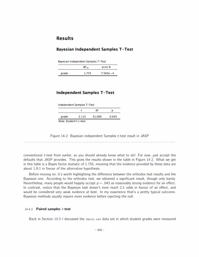
http://www.quotationspage.com/quotes/Ambrosius_Macrobius/

Figure 14.2: Bayesian independent Samples t-test result in JASP

. . . . . . . . . . . . . . . . . . . . . . . . . . . . . . . . . . . . . . . . . . . . . . . . . . . . . . . . . . . . . . . . . . . . . . . . . . . . . . . . . . . . . . . . . . . .

conventional t-test from earlier, so you should already know what to do! For now, just accept thedefaults that JASP provides. This gives the results shown in the table in Figure 14.2. What we getin this table is a Bayes factor statistic of 1.755, meaning that the evidence provided by these data areabout 1.8:1 in favour of the alternative hypothesis.

Before moving on, it’s worth highlighting the difference between the orthodox test results and theBayesian one. According to the orthodox test, we obtained a significant result, though only barely.Nevertheless, many people would happily accept p “ .043 as reasonably strong evidence for an effect.In contrast, notice that the Bayesian test doesn’t even reach 2:1 odds in favour of an effect, andwould be considered very weak evidence at best. In my experience that’s a pretty typical outcome.Bayesian methods usually require more evidence before rejecting the null.

14.4.2 Paired samples t-test

Back in Section 10.5 I discussed the chico.csv data set in which student grades were measured

- 400 -

on two tests, and we were interested in finding out whether grades went up from test 1 to test 2.Because every student did both tests, the tool we used to analyse the data was a paired samplest-test. Figure 14.3 shows the JASP results table for the conventional paired t-test alongside theBayes factor analysis. At this point, I hope you can read this output without any difficulty. The dataprovide evidence of about 6000:1 in favour of the alternative. We could probably reject the null withsome confidence!

Figure 14.3: Paired samples T-Test and Bayes Factor result in JASP

. . . . . . . . . . . . . . . . . . . . . . . . . . . . . . . . . . . . . . . . . . . . . . . . . . . . . . . . . . . . . . . . . . . . . . . . . . . . . . . . . . . . . . . . . . . .

14.5

Summary

The first half of this chapter was focused primarily on the theoretical underpinnings of Bayesianstatistics. I introduced the mathematics for how Bayesian inference works (Section 14.1), and gavea very basic overview of how Bayesian hypothesis testing is typically done (Section 14.2). Finally, Idevoted some space to talking about why I think Bayesian methods are worth using (Section 14.3).

Then I gave a practical example, a Bayesian t-test (Section 14.4). If you’re interested in learningmore about the Bayesian approach, there are many good books you could look into. John Kruschke’s

- 401 -

book Doing Bayesian Data Analysis is a pretty good place to start (Kruschke 2011) and is a nicemix of theory and practice. His approach is a little different to the “Bayes factor” approach that I’vediscussed here, so you won’t be covering the same ground. If you’re a cognitive psychologist, youmight want to check out Michael Lee and E.J. Wagenmakers’ book Bayesian Cognitive Modeling (Leeand Wagenmakers 2014). I picked these two because I think they’re especially useful for people in mydiscipline, but there’s a lot of good books out there, so look around!

!TEX root = ../pdf/lsj.tex

- 402 -

15. Epilogue

“Begin at the beginning”, the King said, very gravely,“and go on till you come to the end: then stop”

– Lewis Carroll

It feels somewhat strange to be writing this chapter, and more than a little inappropriate. Anepilogue is what you write when a book is finished, and this book really isn’t finished. There are a lotof things still missing from this book. It doesn’t have an index yet. A lot of references are missing.There are no “do it yourself” exercises. And in general, I feel that there a lot of things that are wrongwith the presentation, organisation and content of this book. Given all that, I don’t want to try towrite a “proper” epilogue. I haven’t finished writing the substantive content yet, so it doesn’t makesense to try to bring it all together. But this version of the book is going to go online for students touse, and you will may be to purchase a hard copy too, so I want to give it at least a veneer of closure.So let’s give it a go, shall we?

15.1

The undiscovered statistics

First, I’m going to talk a bit about some of the content that I wish I’d had the chance to cram intothis version of the book, just so that you can get a sense of what other ideas are out there in theworld of statistics. I think this would be important even if this book were getting close to a finalproduct. One thing that students often fail to realise is that their introductory statistics classes arejust that, an introduction. If you want to go out into the wider world and do real data analysis, youhave to learn a whole lot of new tools that extend the content of your undergraduate lectures in allsorts of different ways. Don’t assume that something can’t be done just because it wasn’t covered inundergrad. Don’t assume that something is the right thing to do just because it was covered in anundergrad class. To stop you from falling victim to that trap, I think it’s useful to give a bit of anoverview of some of the other ideas out there.

- 403 -

15.1.1 Omissions within the topics covered

Even within the topics that I have covered in the book, there are a lot of omissions that I’d like toredress in future version of the book. Just sticking to things that are purely about statistics (ratherthan things associated with JASP), the following is a representative but not exhaustive list of topicsthat I’d like to expand on at some time:

• Other types of correlations. In Chapter 4 I talked about two types of correlation: Pearson andSpearman. Both of these methods of assessing correlation are applicable to the case where youhave two continuous variables and want to assess the relationship between them. What aboutthe case where your variables are both nominal scale? Or when one is nominal scale and theother is continuous? There are actually methods for computing correlations in such cases (e.g.,polychoric correlation), and it would be good to see these included.

• More detail on effect sizes. In general, I think the treatment of effect sizes throughout thebook is a little more cursory than it should be. In almost every instance, I’ve tended just topick one measure of effect size (usually the most popular one) and describe that. However, foralmost all tests and models there are multiple ways of thinking about effect size, and I’d like togo into more detail in the future.

• Dealing with violated assumptions. In a number of places in the book I’ve talked about somethings you can do when you find that the assumptions of your test (or model) are violated, butI think that I ought to say more about this. In particular, I think it would have been nice to talkin a lot more detail about how you can tranform variables to fix problems. JASP can do somebasic data transformations, but there’s only room to talk about so much in one book!

• Interaction terms for regression. In Chapter 13 I talked about the fact that you can haveinteraction terms in an ANOVA, and I also pointed out that ANOVA can be interpreted as akind of linear regression model. Yet, when talking about regression in Chapter 11 I made notmention of interactions at all. However, there’s nothing stopping you from including interactionterms in a regression model. It’s just a little more complicated to figure out what an “interaction”actually means when you’re talking about the interaction between two continuous predictors,and it can be done in more than one way. Even so, I would have liked to talk a little about this.

• Method of planned comparison. As I mentioned this in Chapter 13, it’s not always appropriateto be using a post hoc correction like Tukey’s HSD when doing an ANOVA, especially when youhad a very clear (and limited) set of comparisons that you cared about ahead of time. I wouldlike to talk more about this in the future.

• Multiple comparison methods. Even within the context of talking about post hoc tests andmultiple comparisons, I would have liked to talk about the methods in more detail, and talkabout what other methods exist besides the few options I mentioned.

- 404 -

15.1.2 Statistical models missing from the book

Statistics is a huge field. The core tools that I’ve described in this book (chi-square tests, t-tests,regression and ANOVA) are basic tools that are widely used in everyday data analysis, and they formthe core of most introductory stats books. However, there are a lot of other tools out there. Thereare so very many data analysis situations that these tools don’t cover, and it would be great to giveyou a sense of just how much more there is, for example:

• Nonlinear regression. When discussing regression in Chapter 11, we saw that regression as-sumes that the relationship between predictors and outcomes is linear. On the other hand, whenwe talked about the simpler problem of correlation in Chapter 4, we saw that there exist tools(e.g., Spearman correlations) that are able to assess non-linear relationships between variables.There are a number of tools in statistics that can be used to do non-linear regression. For in-stance, some non-linear regression models assume that the relationship between predictors andoutcomes is monotonic (e.g., isotonic regression), while others assume that it is smooth butnot necessarily monotonic (e.g., Lowess regression), while others assume that the relationshipis of a known form that happens to be nonlinear (e.g., polynomial regression).

• Logistic regression. Yet another variation on regression occurs when the outcome variableis binary, but the predictors are continuous. For instance, suppose you’re investigating socialmedia, and you want to know if it’s possible to predict whether or not someone is on Twitter asa function of their income, their age, and a range of other variables. This is basically a regressionmodel, but you can’t use regular linear regression because the outcome variable is binary (you’reeither on Twitter or you’re not). Because the outcome variable is binary, there’s no way that theresiduals could possibly be normally distributed. There are a number of tools that statisticianscan apply to this situation, the most prominent of which is logistic regression.

• The General Linear Model (GLM). The GLM is actually a family of models that includeslogistic regression, linear regression, (some) nonlinear regression, ANOVA and many others.The basic idea in the GLM is essentially the same idea that underpins linear models, but itallows for the idea that your data might not be normally distributed, and allows for nonlinearrelationships between predictors and outcomes. There are a lot of very handy analyses that youcan run that fall within the GLM, so it’s a very useful thing to know about.

• Survival analysis. In Chapter 2 I talked about “differential attrition”, the tendency for peopleto leave the study in a non-random fashion. Back then, I was talking about it as a potentialmethodological concern, but there are a lot of situations in which differential attrition is actuallythe thing you’re interested in. Suppose, for instance, you’re interested in finding out how longpeople play different kinds of computer games in a single session. Do people tend to play RTS(real time strategy) games for longer stretches than FPS (first person shooter) games? Youmight design your study like this. People come into the lab, and they can play for as long or aslittle as they like. Once they’re finished, you record the time they spent playing. However, dueto ethical restrictions, let’s suppose that you cannot allow them to keep playing longer than two

- 405 -

hours. A lot of people will stop playing before the two hour limit, so you know exactly how longthey played. But some people will run into the two hour limit, and so you don’t know how longthey would have kept playing if you’d been able to continue the study. As a consequence, yourdata are systematically censored: you’re missing all of the very long times. How do you analysethis data sensibly? This is the problem that survival analysis solves. It is specifically designedto handle this situation, where you’re systematically missing one “side” of the data because thestudy ended. It’s very widely used in health research, and in that context it is often literally usedto analyse survival. For instance, you may be tracking people with a particular type of cancer,some who have received treatment A and others who have received treatment B, but you onlyhave funding to track them for 5 years. At the end of the study period some people are alive,others are not. In this context, survival analysis is useful for determining which treatment ismore effective, and telling you about the risk of death that people face over time.

• Mixed models. Repeated measures ANOVA is often used in situations where you have obser-vations clustered within experimental units. A good example of this is when you track individualpeople across multiple time points. Let’s say you’re tracking happiness over time, for two peo-ple. Aaron’s happiness starts at 10, then drops to 8, and then to 6. Belinda’s happiness startsat 6, then rises to 8 and then to 10. Both of these two people have the same “overall” levelof happiness (the average across the three time points is 8), so a repeated measures ANOVAanalysis would treat Aaron and Belinda the same way. But that’s clearly wrong. Aaron’s happi-ness is decreasing, whereas Belinda’s is increasing. If you want to optimally analyse data froman experiment where people can change over time, then you need a more powerful tool thanrepeated measures ANOVA. The tools that people use to solve this problem are called “mixed”models, because they are designed to learn about individual experimental units (e.g. happinessof individual people over time) as well as overall effects (e.g. the effect of money on happinessover time). Repeated measures ANOVA is perhaps the simplest example of a mixed model, butthere’s a lot you can do with mixed models that you can’t do with repeated measures ANOVA.

• Multidimensional scaling. Factor analysis is an example of an “unsupervised learning” model.What this means is that, unlike most of the “supervised learning” tools I’ve mentioned, you can’tdivide up your variables into predictors and outcomes. Regression is supervised learning whereasfactor analysis is unsupervised learning. It’s not the only type of unsupervised learning modelhowever. For example, in factor analysis one is concerned with the analysis of correlations be-tween variables. However, there are many situations where you’re actually interested in analysingsimilarities or dissimilarities between objects, items or people. There are a number of tools thatyou can use in this situation, the best known of which is multidimensional scaling (MDS). InMDS, the idea is to find a “geometric” representation of your items. Each item is “plotted” as apoint in some space, and the distance between two points is a measure of how dissimilar thoseitems are.

• Clustering. Another example of an unsupervised learning model is clustering (also referred to asclassification), in which you want to organise all of your items into meaningful groups, such thatsimilar items are assigned to the same groups. A lot of clustering is unsupervised, meaning that

- 406 -

you don’t know anything about what the groups are, you just have to guess. There are other“supervised clustering” situations where you need to predict group memberships on the basisof other variables, and those group memberships are actually observables. Logistic regressionis a good example of a tool that works this way. However, when you don’t actually know thegroup memberships, you have to use different tools (e.g., k-means clustering). There are evensituations where you want to do something called “semi-supervised clustering”, in which you knowthe group memberships for some items but not others. As you can probably guess, clustering isa pretty big topic, and a pretty useful thing to know about.

• Causal models. One thing that I haven’t talked about much in this book is how you can usestatistical modelling to learn about the causal relationships between variables. For instance,consider the following three variables which might be of interest when thinking about howsomeone died in a firing squad. We might want to measure whether or not an execution orderwas given (variable A), whether or not a marksman fired their gun (variable B), and whether ornot the person got hit with a bullet (variable C). These three variables are all correlated withone another (e.g., there is a correlation between guns being fired and people getting hit withbullets), but we actually want to make stronger statements about them than merely talkingabout correlations. We want to talk about causation. We want to be able to say that theexecution order (A) causes the marksman to fire (B) which causes someone to get shot (C).We can express this by a directed arrow notation: we write it as A Ñ B Ñ C. This “causalchain” is a fundamentally different explanation for events than one in which the marksman firesfirst, which causes the shooting B Ñ C, and then causes the executioner to “retroactively” issuethe execution order, B Ñ A. This “common effect” model says that A and C are both causedby B. You can see why these are different. In the first causal model, if we had managed tostop the executioner from issuing the order (intervening to change A), then no shooting wouldhave happened. In the second model, the shooting would have happened any way because themarksman was not following the execution order. There is a big literature in statistics on tryingto understand the causal relationships between variables, and a number of different tools existto help you test different causal stories about your data. The most widely used of these tools(in psychology at least) is structural equations modelling (SEM), and at some point I’d like toextend the book to talk about it.

Of course, even this listing is incomplete. I haven’t mentioned time series analysis, item responsetheory, market basket analysis, classification and regression trees, or any of a huge range of othertopics. However, the list that I’ve given above is essentially my wish list for this book. Sure, it woulddouble the length of the book, but it would mean that the scope has become broad enough to covermost things that applied researchers in psychology would need to use.

15.1.3 Other ways of doing inference

A different sense in which this book is incomplete is that it focuses pretty heavily on a very narrow andold-fashioned view of how inferential statistics should be done. In Chapter 7 I talked a little bit about

- 407 -

the idea of unbiased estimators, sampling distributions and so on. In Chapter 8 I talked about thetheory of null hypothesis significance testing and p-values. These ideas have been around since theearly 20th century, and the tools that I’ve talked about in the book rely very heavily on the theoreticalideas from that time. I’ve felt obligated to stick to those topics because the vast majority of dataanalysis in science is also reliant on those ideas. However, the theory of statistics is not restrictedto those topics and, whilst everyone should know about them because of their practical importance,in many respects those ideas do not represent best practice for contemporary data analysis. One ofthe things that I’m especially happy with is that I’ve been able to go a little beyond this. Chapter 14now presents the Bayesian perspective in a reasonable amount of detail, but the book overall is stillpretty heavily weighted towards the frequentist orthodoxy. Additionally, there are a number of otherapproaches to inference that are worth mentioning:

• Bootstrapping. Throughout the book, whenever I’ve introduced a hypothesis test, I’ve hada strong tendency just to make assertions like “the sampling distribution for BLAH is a t-distribution” or something like that. In some cases, I’ve actually attempted to justify thisassertion. For example, when talking about χ2 tests in Chapter 9 I made reference to theknown relationship between normal distributions and χ2 distributions (see Chapter 6) to explainhow we end up assuming that the sampling distribution of the goodness-of-fit statistic is χ2.However, it’s also the case that a lot of these sampling distributions are, well, wrong. The χ2

test is a good example. It is based on an assumption about the distribution of your data, anassumption which is known to be wrong for small sample sizes! Back in the early 20th century,there wasn’t much you could do about this situation. Statisticians had developed mathematicalresults that said that “under assumptions BLAH about the data, the sampling distribution isapproximately BLAH”, and that was about the best you could do. A lot of times they didn’t evenhave that. There are lots of data analysis situations for which no-one has found a mathematicalsolution for the sampling distributions that you need. And so up until the late 20th century, thecorresponding tests didn’t exist or didn’t work. However, computers have changed all that now.There are lots of fancy tricks, and some not-so-fancy, that you can use to get around it. Thesimplest of these is bootstrapping, and in it’s simplest form it’s incredibly simple. What you dois simulate the results of your experiment lots and lots of times, under the twin assumptions that(a) the null hypothesis is true and (b) the unknown population distribution actually looks prettysimilar to your raw data. In other words, instead of assuming that the data are (for instance)normally distributed, just assume that the population looks the same as your sample, and thenuse computers to simulate the sampling distribution for your test statistic if that assumptionholds. Despite relying on a somewhat dubious assumption (i.e., the population distribution isthe same as the sample!) bootstrapping is quick and easy method that works remarkably wellin practice for lots of data analysis problems.

• Cross validation. One question that pops up in my stats classes every now and then, usuallyby a student trying to be provocative, is “Why do we care about inferential statistics at all?Why not just describe your sample?” The answer to the question is usually something like this,“Because our true interest as scientists is not the specific sample that we have observed in thepast, we want to make predictions about data we might observe in the future”. A lot of the

- 408 -

issues in statistical inference arise because of the fact that we always expect the future to besimilar to but a bit different from the past. Or, more generally, new data won’t be quite thesame as old data. What we do, in a lot of situations, is try to derive mathematical rules thathelp us to draw the inferences that are most likely to be correct for new data, rather than topick the statements that best describe old data. For instance, given two models A and B, anda data set X you collected today, try to pick the model that will best describe a new data set Ythat you’re going to collect tomorrow. Sometimes it’s convenient to simulate the process, andthat’s what cross-validation does. What you do is divide your data set into two subsets, X1 andX2. Use the subset X1 to train the model (e.g., estimate regression coefficients, let’s say), butthen assess the model performance on the other one X2. This gives you a measure of how wellthe model generalises from an old data set to a new one, and is often a better measure of howgood your model is than if you just fit it to the full data set X.

• Robust statistics. Life is messy, and nothing really works the way it’s supposed to. This is just astrue for statistics as it is for anything else, and when trying to analyse data we’re often stuck withall sorts of problems in which the data are just messier than they’re supposed to be. Variablesthat are supposed to be normally distributed are not actually normally distributed, relationshipsthat are supposed to be linear are not actually linear, and some of the observations in your dataset are almost certainly junk (i.e., not measuring what they’re supposed to). All of this messinessis ignored in most of the statistical theory I developed in this book. However, ignoring a problemdoesn’t always solve it. Sometimes, it’s actually okay to ignore the mess, because some typesof statistical tools are “robust”, i.e., if the data don’t satisfy your theoretical assumptions theynevertheless still work pretty well. Other types of statistical tools are not robust, and even minordeviations from the theoretical assumptions cause them to break. Robust statistics is a branchof stats concerned with this question, and they talk about things like the “breakdown point” of astatistic. That is, how messy does your data have to be before the statistic cannot be trusted?I touched on this in places. The mean is not a robust estimator of the central tendency of avariable, but the median is. For instance, suppose I told you that the ages of my five best friendsare 34, 39, 31, 43 and 4003 years. How old do you think they are on average? That is, what isthe true population mean here? If you use the sample mean as your estimator of the populationmean, you get an answer of 830 years. If you use the sample median as the estimator of thepopulation mean, you get an answer of 39 years. Notice that, even though you’re “technically”doing the wrong thing in the second case (using the median to estimate the mean!) you’reactually getting a better answer. The problem here is that one of the observations is clearly,obviously, a lie. I don’t have a friend aged 4003 years. It’s probably a typo, I probably meant totype 43. But what if I had typed 53 instead of 43, or 34 instead of 43? Could you be sure ifthis was a typo or not? Sometimes the errors in the data are subtle, so you can’t detect themjust by eyeballing the sample, but they’re still errors that contaminate your data, and they stillaffect your conclusions. Robust statistics is concerned with how you can make safe inferenceseven when faced with contamination that you don’t know about. It’s pretty cool stuff.

- 409 -

15.1.4 Miscellaneous topics

• Missing data. Suppose you’re doing a survey, and you’re interested in exercise and weight. Yousend data to four people. Adam says he exercises a lot and is not overweight. Briony says sheexercises a lot and is not overweight. Carol says she does not exercise and is overweight. Dansays he does not exercise and refuses to answer the question about his weight. Elaine does notreturn the survey. You now have a missing data problem. There is one entire survey missing,and one question missing from another one, What do you do about it? Ignoring missing datais not, in general, a safe thing to do. Let’s think about Dan’s survey here. Firstly, notice that,on the basis of my other responses, I appear to be more similar to Carol (neither of us exercise)than to Adam or Briony. So if you were forced to guess my weight, you’d guess that I’m closerto her than to them. Maybe you’d make some correction for the fact that Adam and I are malesand Briony and Carol are females. The statistical name for this kind of guessing is “imputation”.Doing imputation safely is hard, but it’s important, especially when the missing data are missingin a systematic way. Because of the fact that people who are overweight are often pressuredto feel poorly about their weight (often thanks to public health campaigns), we actually havereason to suspect that the people who are not responding are more likely to be overweight thanthe people who do respond. Imputing a weight to Dan means that the number of overweightpeople in the sample will probably rise from 1 out of 3 (if we ignore Dan), to 2 out of 4 (if weimpute Dan’s weight). Clearly this matters. But doing it sensibly is more complicated than itsounds. Earlier, I suggested you should treat me like Carol, since we gave the same answer to theexercise question. But that’s not quite right. There is a systematic difference between us. Sheanswered the question, and I didn’t. Given the social pressures faced by overweight people, isn’tit likely that I’m more overweight than Carol? And of course this is still ignoring the fact that it’snot sensible to impute a single weight to me, as if you actually knew my weight. Instead, whatyou need to do it is impute a range of plausible guesses (referred to as multiple imputation),in order to capture the fact that you’re more uncertain about my weight than you are aboutCarol’s. And let’s not get started on the problem posed by the fact that Elaine didn’t send inthe survey. As you can probably guess, dealing with missing data is an increasingly importanttopic. In fact, I’ve been told that a lot of journals in some fields will not accept studies thathave missing data unless some kind of sensible multiple imputation scheme is followed.

• Power analysis. In Chapter 8 I discussed the concept of power (i.e., how likely are you to beable to detect an effect if it actually exists) and referred to power analysis, a collection of toolsthat are useful for assessing how much power your study has. Power analysis can be usefulfor planning a study (e.g., figuring out how large a sample you’re likely to need), but it alsoserves a useful role in analysing data that you already collected. For instance, suppose you geta significant result, and you have an estimate of your effect size. You can use this informationto estimate how much power your study actually had. This is kind of useful, especially if youreffect size is not large. For instance, suppose you reject the null hypothesis at p ă .05, butyou use power analysis to figure out that your estimated power was only .08. The significantresult means that, if the null hypothesis was in fact true, there was a 5% chance of getting data

- 410 -

like this. But the low power means that, even if the null hypothesis is false and the effect sizewas really as small as it looks, there was only an 8% chance of getting data like you did. Thissuggests that you need to be pretty cautious, because luck seems to have played a big part inyour results, one way or the other!

• Data analysis using theory-inspired models. In a few places in this book I’ve mentionedresponse time (RT) data, where you record how long it takes someone to do something (e.g.,make a simple decision). I’ve mentioned that RT data are almost invariably non-normal, andpositively skewed. Additionally, there’s a thing known as the speed-accuracy trade-off: if youtry to make decisions too quickly (low RT) then you’re likely to make poorer decisions (loweraccuracy). So if you measure both the accuracy of a participant’s decisions and their RT, you’llprobably find that speed and accuracy are related. There’s more to the story than this, ofcourse, because some people make better decisions than others regardless of how fast they’regoing. Moreover, speed depends on both cognitive processes (i.e., time spent thinking) butalso physiological ones (e.g., how fast can you move your muscles). It’s starting to sound likeanalysing this data will be a complicated process. And indeed it is, but one of the things that youfind when you dig into the psychological literature is that there already exist mathematical models(called “sequential sampling models”) that describe how people make simple decisions, and thesemodels take into account a lot of the factors I mentioned above. You won’t find any of thesetheoretically-inspired models in a standard statistics textbook. Standard stats textbooks describestandard tools, tools that could meaningfully be applied in lots of different disciplines, not justpsychology. ANOVA is an example of a standard tool that is just as applicable to psychologyas to pharmacology. Sequential sampling models are not, they are psychology-specific, moreor less. This doesn’t make them less powerful tools. In fact, if you’re analysing data wherepeople have to make choices quickly you should really be using sequential sampling models toanalyse the data. Using ANOVA or regression or whatever won’t work as well, because thetheoretical assumptions that underpin them are not well-matched to your data. In contrast,sequential sampling models were explicitly designed to analyse this specific type of data, andtheir theoretical assumptions are extremely well-matched to the data.

15.2

Learning the basics, and learning them in JASP

Okay, that was a long list. And even that listing is massively incomplete. There really are a lot ofbig ideas in statistics that I haven’t covered in this book. It can seem pretty depressing to finish analmost 500-page textbook only to be told that this is only the beginning, especially when you start tosuspect that half of the stuff you’ve been taught is wrong. For instance, there are a lot of people inthe field who would strongly argue against the use of the classical ANOVA model, yet I’ve devotedtwo whole chapters to it! Standard ANOVA can be attacked from a Bayesian perspective, or from arobust statistics perspective, or even from a “it’s just plain wrong” perspective (people very frequently

- 411 -

use ANOVA when they should actually be using mixed models). So why learn it at all?

As I see it, there are two key arguments. Firstly, there’s the pure pragmatism argument. Rightlyor wrongly, ANOVA is widely used. If you want to understand the scientific literature, you need tounderstand ANOVA. And secondly, there’s the “incremental knowledge” argument. In the same waythat it was handy to have seen one-way ANOVA before trying to learn factorial ANOVA, understandingANOVA is helpful for understanding more advanced tools, because a lot of those tools extend on ormodify the basic ANOVA setup in some way. For instance, although mixed models are way more usefulthan ANOVA and regression, I’ve never heard of anyone learning how mixed models work without firsthaving worked through ANOVA and regression. You have to learn to crawl before you can climb amountain.

Actually, I want to push this point a bit further. One thing that I’ve done a lot of in this bookis talk about fundamentals. I spent a lot of time on probability theory. I talked about the theoryof estimation and hypothesis tests in more detail than I needed to. Why did I do all this? Lookingback, you might ask whether I really needed to spend all that time talking about what a probabilitydistribution is, or why there was even a section on probability density. If the goal of the book was toteach you how to run a t-test or an ANOVA, was all that really necessary? Was this all just a hugewaste of everyone’s time???

The answer, I hope you’ll agree, is no. The goal of an introductory stats is not to teach ANOVA.It’s not to teach t-tests, or regressions, or histograms, or p-values. The goal is to start you onthe path towards becoming a skilled data analyst. And in order for you to become a skilled dataanalyst, you need to be able to do more than ANOVA, more than t-tests, regressions and histograms.You need to be able to think properly about data. You need to be able to learn the more advancedstatistical models that I talked about in the last section, and to understand the theory upon whichthey are based. And you need to have access to software that will let you use those advanced tools.And this is where, in my opinion at least, all that extra time I’ve spent on the fundamentals pays off.If you understand probability theory, you’ll find it much easier to switch from frequentist analyses toBayesian ones.

In short, I think that the big payoff for learning statistics this way is extensibility. For a book thatonly covers the very basics of data analysis, this book has a massive overhead in terms of learningprobability theory and so on. There’s a whole lot of other things that it pushes you to learn besidesthe specific analyses that the book covers. So if your goal had been to learn how to run an ANOVAin the minimum possible time, well, this book wasn’t a good choice. But as I say, I don’t think thatis your goal. I think you want to learn how to do data analysis. And if that really is your goal, youwant to make sure that the skills you learn in your introductory stats class are naturally and cleanlyextensible to the more complicated models that you need in real world data analysis. You want tomake sure that you learn to use the same tools that real data analysts use, so that you can learn todo what they do. And so yeah, okay, you’re a beginner right now (or you were when you started thisbook), but that doesn’t mean you should be given a dumbed-down story, a story in which I don’t tellyou about probability density, or a story where I don’t tell you about the nightmare that is factorialANOVA with unbalanced designs. And it doesn’t mean that you should be given baby toys instead ofproper data analysis tools. Beginners aren’t dumb, they just lack knowledge. What you need is not

- 412 -

to have the complexities of real world data analysis hidden from from you. What you need are theskills and tools that will let you handle those complexities when they inevitably ambush you in the realworld.

And what I hope is that this book, or the finished book that this will one day turn into, is able tohelp you with that.

- 413 -

Author’s note – I’ve mentioned it before, but I’ll quickly mention it again. This reference list isappallingly incomplete. Please don’t assume that these are the only sources I’ve relied upon. The finalversion of this book will have a lot more references. And if you see anything clever sounding in thisbook that doesn’t seem to have a reference, I can absolutely promise you that the idea was someoneelse’s. This is an introductory textbook: none of the ideas are original. I’ll take responsibility for allthe errors, but I can’t take credit for any of the good stuff. Everything smart in this book came fromsomeone else, and they all deserve proper attribution for their excellent work. I just haven’t had thechance to give it to them yet.

- 414 -

16. References

Adair, G. (1984). “The Hawthorne effect: A reconsideration of the methodological artifact”. In: Journalof Applied Psychology 69, pp. 334–345 (page 37).

Agresti, A. (1996). An Introduction to Categorical Data Analysis. Hoboken, New Jersey: Wiley(page 206).

— (2002). Categorical Data Analysis. 2nd. Hoboken, New Jersey: Wiley (page 206).Akaike, H. (1974). “A new look at the statistical model identification”. In: IEEE Transactions on

Automatic Control 19, pp. 716–723 (page 289).Anscombe, F. J. (1973). “Graphs in statistical analysis”. In: American Statistician 27, pp. 17–21

(page 257).Bickel, P. J., E. A. Hammel, and J. W. O’Connell (1975). “Sex bias in graduate admissions: Data

from Berkeley”. In: Science 187, pp. 398–404 (pages 7, 8).Box, G. E. P. (1953). “Non-normality and tests on variances”. In: Biometrika 40, pp. 318–335

(page 312).Box, George E. P. (1976). “Science and Statistics”. In: Journal of the American Statistical Association

71, pp. 791–799 (page 172).Box, J. F. (1987). “Guinness, Gosset, Fisher, and Small Samples”. In: Statistical Science 2, pp. 45–52

(page 215).Brown, M. B. and A. B. Forsythe (1974). “Robust tests for equality of variances”. In: Journal of the

American Statistical Association 69, pp. 364–367 (page 312).Campbell, D. T. and J. C. Stanley (1963). Experimental and Quasi-Experimental Designs for Research.

Boston, MA: Houghton Mifflin (pages 13, 41).Cochran, W. G. (1954). “The χ2 test of goodness of fit”. In: The Annals of Mathematical Statistics

23, pp. 315–345 (page 205).Cohen, J. (1988). Statistical Power Analysis for the Behavioral Sciences. 2nd. Lawrence Erlbaum

(pages 172, 238).Cramer, H. (1946).Mathematical Methods of Statistics. Princeton: Princeton University Press (page 204).Dunn, O.J. (1961). “Multiple comparisons among means”. In: Journal of the American Statistical

Association 56, pp. 52–64 (pages 309, 310).Ellis, P. D. (2010). The Essential Guide to Effect Sizes: Statistical Power, Meta-Analysis, and the

Interpretation of Research Results. Cambridge, UK: Cambridge University Press (page 172).

- 415 -

Ellman, Michael (2002). “Soviet repression statistics: some comments”. In: Europe-Asia Studies 54.7,pp. 1151–1172 (page 79).

Evans, J. St. B. T., J. L. Barston, and P. Pollard (1983). “On the conflict between logic and belief insyllogistic reasoning”. In: Memory and Cognition 11, pp. 295–306 (page 5).

Evans, M., N. Hastings, and B. Peacock (2011). Statistical Distributions (3rd ed). New York, NY:Wiley (page 122).

Everitt, Brian S. (1996). Making Sense of Statistics in Psychology. A Second-Level Course. OxfordUniversity Press (page 351).

Fisher, R. A. (1922a). “On the interpretation of χ2 from contingency tables, and the calculation ofp”. In: Journal of the Royal Statistical Society 84, pp. 87–94 (page 183).

— (1922b). “On the mathematical foundation of theoretical statistics”. In: Philosophical Transactionsof the Royal Society A 222, pp. 309–368 (page 106).

— (1925). Statistical Methods for Research Workers. Edinburgh, UK: Oliver & Boyd (page 393).Fox, J. and S. Weisberg (2011). An R Companion to Applied Regression. 2nd. Los Angeles: Sage

(page 281).Gelman, A. and H. Stern (2006). “The difference between “significant” and “not significant” is not

itself statistically significant”. In: The American Statistician 60, pp. 328–331 (page 179).Gelman, Andrew and Eric Loken (2014). “The statistical crisis in science”. In: American Scientist

102.6, pp. 460+. issn: 0003-0996. doi: 10.1511/2014.111.460. url: http://mfkp.org/INRMM/article/13469628 (page 39).

Geschwind, N. (1972). “Language and the brain”. In: Scientific American 226(4), pp. 76–83 (page 320).Hays, W. L. (1994). Statistics. 5th. Fort Worth, TX: Harcourt Brace (page 301).Hedges, L. V. (1981). “Distribution theory for Glass’s estimator of effect size and related estimators”.

In: Journal of Educational Statistics 6, pp. 107–128 (page 240).Hedges, L. V. and I. Olkin (1985). Statistical Methods for Meta-Analysis. New York: Academic Press

(page 241).Hogg, R. V., J. V. McKean, and A. T. Craig (2005). Introduction to Mathematical Statistics. 6th.

Upper Saddle River, NJ: Pearson (page 199).Holm, S. (1979). “A simple sequentially rejective multiple test procedure”. In: Scandinavian Journal of

Statistics 6, pp. 65–70 (page 310).Hothersall, D. (2004). History of Psychology. McGraw-Hill (page 36).Hróbjartsson, A and PC Gøtzsche (2010). “Placebo interventions for all clinical conditions”. In:

Cochrane Database of Systematic Reviews 1. url: https://doi.org//10.1002/14651858.CD003974.pub3 (page 37).

Hsu, J. C. (1996). Multiple Comparisons: Theory and Methods. London, UK: Chapman and Hall(pages 309, 366).

Ioannidis, John P. A. (2005). “Why Most Published Research Findings Are False”. In: PLoS Med 2.8,pp. 697–701 (page 40).

Jeffreys, Harold (1961). The Theory of Probability. 3rd. Oxford (page 390).Johnson, Valen E (2013). “Revised standards for statistical evidence”. In: Proceedings of the National

Academy of Sciences 48, pp. 19313–19317 (pages 393, 394, 396).

- 416 -

https://doi.org/10.1511/2014.111.460

http://mfkp.org/INRMM/article/13469628

http://mfkp.org/INRMM/article/13469628

https://doi.org//10.1002/14651858.CD003974.pub3

https://doi.org//10.1002/14651858.CD003974.pub3

Kahneman, D. and A. Tversky (1973). “On the psychology of prediction”. In: Psychological Review80, pp. 237–251 (page 35).

Kass, Robert E. and Adrian E. Raftery (1995). “Bayes factors”. In: Journal of the American StatisticalAssociation 90, pp. 773–795 (pages 390, 391).

Keynes, John Maynard (1923). A Tract on Monetary Reform. London: Macmillan and Company(page 133).

Kruschke, J. K. (2011). Doing Bayesian Data Analysis: A Tutorial with R and BUGS. Burlington, MA:Academic Press (page 402).

Kruskal, W. H. and W. A. Wallis (1952). “Use of ranks in one-criterion variance analysis”. In: Journalof the American Statistical Association 47, pp. 583–621 (page 315).

Kühberger, A, A Fritz, and T. Scherndl (2014). “Publication bias in psychology: A diagnosis based onthe correlation between effect size and sample size”. In: Public Library of Science One 9, pp. 1–8(page 40).

Larntz, K. (1978). “Small-sample comparisons of exact levels for chi-squared goodness-of-fit statistics”.In: Journal of the American Statistical Association 73, pp. 253–263 (page 205).

Lee, Michael D and Eric-Jan Wagenmakers (2014). Bayesian cognitive modeling: A practical course.Cambridge University Press (page 402).

Lehmann, Erich L. (2011). Fisher, Neyman, and the Creation of Classical Statistics. Springer (page 177).Levene, H (1960). “Robust tests for equality of variances”. In: Contributions to Probability and Statis-

tics: Essays in Honor of Harold Hotelling. Ed. by I. Olkin et al. Palo Alto, CA: Stanford UniversityPress, pp. 278–292 (page 312).

McGrath, R. E. and G. J. Meyer (2006). “When effect sizes disagree: The case of r and d ”. In:Psychological Methods 11, pp. 386–401 (page 239).

Meehl, P. H. (1967). “Theory testing in psychology and physics: A methodological paradox”. In:Philosophy of Science 34, pp. 103–115 (page 106).

Pearson, K. (1900). “On the criterion that a given system of deviations from the probable in the caseof a correlated system of variables is such that it can be reasonably supposed to have arisen fromrandom sampling”. In: Philosophical Magazine 50, pp. 157–175 (page 183).

Pfungst, O. (1911). Clever Hans (The horse of Mr. von Osten): A contribution to experimental animaland human psychology. Trans. by C. L. Rahn. New York: Henry Holt (page 36).

Rosenthal, R (1966). Experimenter effects in behavioral research. New York: Appleton (page 36).Sahai, H. and M. I. Ageel (2000). The Analysis of Variance: Fixed, Random and Mixed Models. Boston:

Birkhauser (page 326).Shaffer, J. P. (1995). “Multiple hypothesis testing”. In: Annual Review of Psychology 46, pp. 561–584

(page 309).Shapiro, S. S. and M. B. Wilk (1965). “An analysis of variance test for normality (complete samples)”.

In: Biometrika 52, pp. 591–611 (page 244).Sokal, R. R. and F. J. Rohlf (1994). Biometry: the principles and practice of statistics in biological

research. 3rd. New York: Freeman (page 196).Stevens, S. S. (1946). “On the theory of scales of measurement”. In: Science 103, pp. 677–680

(page 13).Stigler, S. M. (1986). The History of Statistics. Cambridge, MA: Harvard University Press (page 131).

- 417 -

Student, A. (1908). “The probable error of a mean”. In: Biometrika 6, pp. 1–2 (page 215).Welch, B. L. (1947). “The generalization of “Student’s” problem when several different population

variances are involved”. In: Biometrika 34, pp. 28–35 (page 229).— (1951). “On the comparison of several mean values: An alternative approach”. In: Biometrika 38,

pp. 330–336 (page 314).Wilkinson, Leland et al. (2006). The grammar of graphics. Springer (page 90).Yates, F. (1934). “Contingency tables involving small numbers and the χ2 test”. In: Supplement to

the Journal of the Royal Statistical Society 1, pp. 217–235 (page 203).

- 418 -

learning statistics with jasplearning statistics with jasp: a tutorial for psychology students and...

Documents