learning curve supplement_ch07.pdf

SUPPLEMENT OUTLINEThe Concept of Learning

Curves, 7S-2

Determining the Learning Percentage, 7S-6

Applications of Learning Curves, 7S-7

Cautions and Criticisms, 7S-9

Summary, 7S-9

Solved Problems, 7S-10

Discussion and Review Questions, 7S-11

Internet Exercise, 7S-11

Problems, 7S-11

Mini-Case: Product Recall, 7S-14

Mini-Case: Learning Curve inSurgery, 7S-14

Case: Renovating the Lions GateBridge, 7S-15

Selected Bibliography and FurtherReading, 7S-19

Learning Curves

LEARNING OBJECTIVES

After completing this supplement,you should be able to:

1 Explain the concept of alearning curve.

2 Make time estimates based onlearning curves.

3 Determining the learningpercentage.

4 List and briefly describe someof the main applications oflearning curves.

5 Outline some of the cautionsand criticisms of learningcurves.

7S-1

SUPPLEMENT TO

CHAPTER7

ste51675_ch07_suppl.qxd 10/11/2006 3:25 PM Page 7S-1

L earning usually occurs when humans are involved; this is a basic consideration in thedesign of work systems. It is important to be able to predict how learning will affect

task times and costs. This supplement addresses those issues.

THE CONCEPT OF LEARNING CURVESHuman performance of activities typically shows improvement when the activities aredone on a repetitive basis: The time required to perform a task decreases with increasingrepetitions. Learning curves summarize this phenomenon. The degree of improvementand the number of tasks needed to realize the major portion of the improvement is a func-tion of the task being done. If the task is short and somewhat routine, only a modestamount of improvement is likely to occur, and it generally occurs during the first few rep-etitions. If the task is fairly complex and has a longer duration, improvements will occurover a longer interval (i.e., a larger number of repetitions). Therefore, learning factorshave little relevance for planning or scheduling routine activities, but they do have rele-vance for complex repetitive activities.

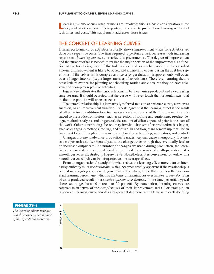
Figure 7S–1 illustrates the basic relationship between units produced and a decreasingtime per unit. It should be noted that the curve will never touch the horizontal axis; thatis, the time per unit will never be zero.

The general relationship is alternatively referred to as an experience curve, a progressfunction, or an improvement function. Experts agree that the learning effect is the resultof other factors in addition to actual worker learning. Some of the improvement can betraced to preproduction factors, such as selection of tooling and equipment, product de-sign, methods analysis, and, in general, the amount of effort expended prior to the start ofthe work. Other contributing factors may involve changes after production has begun,such as changes in methods, tooling, and design. In addition, management input can be animportant factor through improvements in planning, scheduling, motivation, and control.

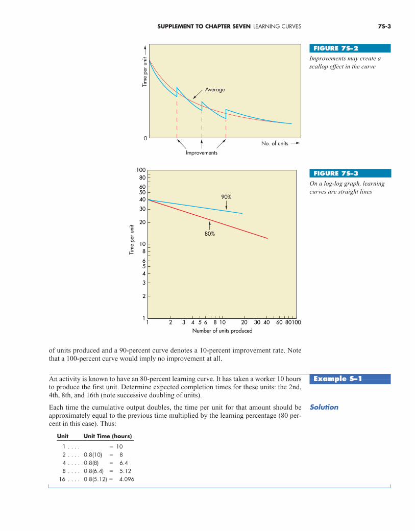
Changes that are made once production is under way can cause a temporary increasein time per unit until workers adjust to the change, even though they eventually lead toan increased output rate. If a number of changes are made during production, the learn-ing curve would be more realistically described by a series of scallops instead of asmooth curve, as illustrated in Figure 7S–2. Nonetheless, it is convenient to work with asmooth curve, which can be interpreted as the average effect.

From an organizational standpoint, what makes the learning effect more than an inter-esting curiosity is its predictability, which becomes readily apparent if the relationship isplotted on a log-log scale (see Figure 7S–3). The straight line that results reflects a con-stant learning percentage, which is the basis of learning curve estimates: Every doublingof units produced results in a constant percentage decrease in the time per unit. Typicaldecreases range from 10 percent to 20 percent. By convention, learning curves are referred to in terms of the complements of their improvement rates. For example, an 80-percent learning curve denotes a 20-percent decrease in unit time with each doubling

7S-2 SUPPLEMENT TO CHAPTER SEVEN LEARNING CURVES

Number of units

Tim

e pe

r un

it

0

FIGURE 7S–1

The learning effect: time perunit decreases as the numberof units produced increases


of units produced and a 90-percent curve denotes a 10-percent improvement rate. Notethat a 100-percent curve would imply no improvement at all.

An activity is known to have an 80-percent learning curve. It has taken a worker 10 hoursto produce the first unit. Determine expected completion times for these units: the 2nd,4th, 8th, and 16th (note successive doubling of units).

Each time the cumulative output doubles, the time per unit for that amount should be approximately equal to the previous time multiplied by the learning percentage (80 per-cent in this case). Thus:

Unit Unit Time (hours)

1 . . . . � 102 . . . . 0.8(10) � 84 . . . . 0.8(8) � 6.48 . . . . 0.8(6.4) � 5.12

16 . . . . 0.8(5.12) � 4.096

SUPPLEMENT TO CHAPTER SEVEN LEARNING CURVES 7S-3

No. of unitsTi

me

per

unit

0

Improvements

Average

FIGURE 7S–2

Improvements may create ascallop effect in the curve

Number of units produced

Tim

e pe

r un

it

1

10080

605040

30

20

108

654

3

2

1 2 3 4 5 6 8 10 20 30 40 10060

90%

80%

80

FIGURE 7S–3

On a log-log graph, learningcurves are straight lines

Example S–1

Solution


Example S–1 illustrates an important point and also raises an interesting question. Thepoint is that the time reduction per unit becomes less and less as the number of units produced increases. For example, the second unit required two hours less time than thefirst, and the improvement from the 8th to the 16th unit was only slightly more than onehour. The question raised is: How are times computed for values such as three, five, six,seven, and other units that don’t fall into this pattern?

There are two ways to obtain the times. One is to use a formula; the other is to use atable of values.

First, consider the formula approach. The formula is based on the existence of a linearrelationship between the time per unit and the number of units when these two variablesare expressed in logarithms.

The unit time (i.e., the number of direct labour hours required) for the nth unit can becomputed using the formula

Tn � T1 � nb (7S–1)

where

Tn � Time for nth unit

T1 � Time for first unit

b � 1n stands for the natural logarithm

To use the formula, you need to know the time for the first unit and the learning per-centage. For example, for an 80-percent curve with T1�10 hours, the time for the thirdunit would be computed as

T3 � 10(31n.8/1n 2) � 7.02

Values of b for various values of learning percentage are given below:

LearningPercentage b

70 6.12975 6.22980 6.32285 6.40990 6.492

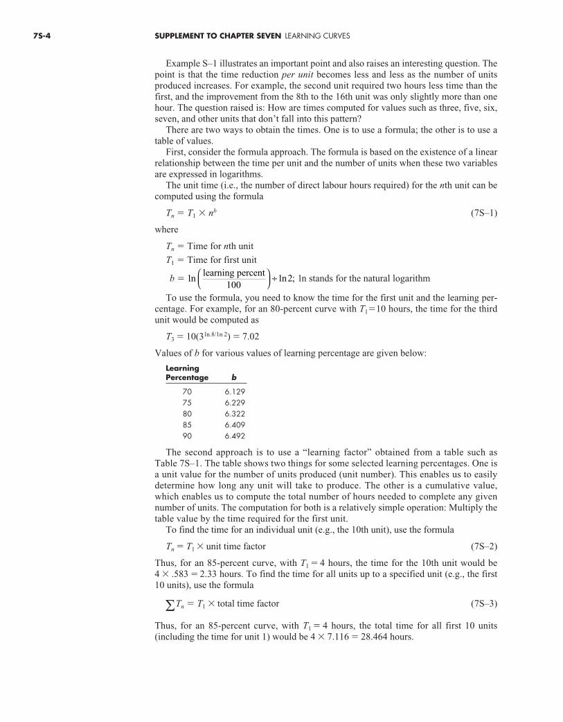
The second approach is to use a “learning factor” obtained from a table such asTable 7S–1. The table shows two things for some selected learning percentages. One isa unit value for the number of units produced (unit number). This enables us to easilydetermine how long any unit will take to produce. The other is a cumulative value,which enables us to compute the total number of hours needed to complete any givennumber of units. The computation for both is a relatively simple operation: Multiply thetable value by the time required for the first unit.

To find the time for an individual unit (e.g., the 10th unit), use the formula

Tn � T1 � unit time factor (7S–2)

Thus, for an 85-percent curve, with T1 � 4 hours, the time for the 10th unit would be4 � .583 � 2.33 hours. To find the time for all units up to a specified unit (e.g., the first10 units), use the formula

ΣTn � T1 � total time factor (7S–3)

Thus, for an 85-percent curve, with T1 � 4 hours, the total time for all first 10 units (including the time for unit 1) would be 4 � 7.116 � 28.464 hours.

1 1 2n n ;learning percent

100

÷




An airplane manufacturer is negotiating a contract for the production of 20 small jet aircraft. The initial jet required the equivalent of 400 days of direct labour. The learningpercentage is 80 percent. Estimate the expected number of days of direct labour for:

a. The 20th jet.

b. All 20 jets.

c. The average time for 20 jets.

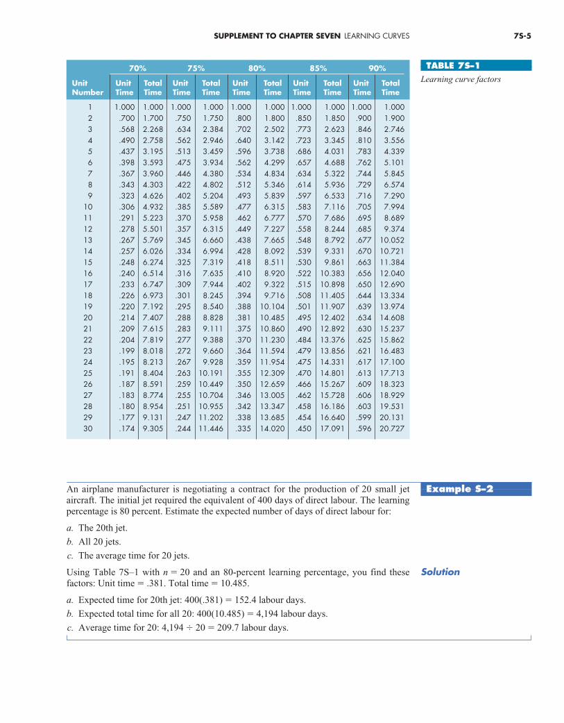
Using Table 7S–1 with n � 20 and an 80-percent learning percentage, you find these factors: Unit time � .381. Total time � 10.485.

a. Expected time for 20th jet: 400(.381) � 152.4 labour days.

b. Expected total time for all 20: 400(10.485) � 4,194 labour days.

c. Average time for 20: 4,194 � 20 � 209.7 labour days.

Example S–2

Solution

70% 75% 80% 85% 90%

Unit Unit Total Unit Total Unit Total Unit Total Unit TotalNumber Time Time Time Time Time Time Time Time Time Time

1 1.000 1.000 1.000 1.000 1.000 1.000 1.000 1.000 1.000 1.0002 .700 1.700 .750 1.750 .800 1.800 .850 1.850 .900 1.9003 .568 2.268 .634 2.384 .702 2.502 .773 2.623 .846 2.7464 .490 2.758 .562 2.946 .640 3.142 .723 3.345 .810 3.5565 .437 3.195 .513 3.459 .596 3.738 .686 4.031 .783 4.3396 .398 3.593 .475 3.934 .562 4.299 .657 4.688 .762 5.1017 .367 3.960 .446 4.380 .534 4.834 .634 5.322 .744 5.8458 .343 4.303 .422 4.802 .512 5.346 .614 5.936 .729 6.5749 .323 4.626 .402 5.204 .493 5.839 .597 6.533 .716 7.290

10 .306 4.932 .385 5.589 .477 6.315 .583 7.116 .705 7.99411 .291 5.223 .370 5.958 .462 6.777 .570 7.686 .695 8.68912 .278 5.501 .357 6.315 .449 7.227 .558 8.244 .685 9.37413 .267 5.769 .345 6.660 .438 7.665 .548 8.792 .677 10.05214 .257 6.026 .334 6.994 .428 8.092 .539 9.331 .670 10.72115 .248 6.274 .325 7.319 .418 8.511 .530 9.861 .663 11.38416 .240 6.514 .316 7.635 .410 8.920 .522 10.383 .656 12.04017 .233 6.747 .309 7.944 .402 9.322 .515 10.898 .650 12.69018 .226 6.973 .301 8.245 .394 9.716 .508 11.405 .644 13.33419 .220 7.192 .295 8.540 .388 10.104 .501 11.907 .639 13.97420 .214 7.407 .288 8.828 .381 10.485 .495 12.402 .634 14.60821 .209 7.615 .283 9.111 .375 10.860 .490 12.892 .630 15.23722 .204 7.819 .277 9.388 .370 11.230 .484 13.376 .625 15.86223 .199 8.018 .272 9.660 .364 11.594 .479 13.856 .621 16.48324 .195 8.213 .267 9.928 .359 11.954 .475 14.331 .617 17.10025 .191 8.404 .263 10.191 .355 12.309 .470 14.801 .613 17.71326 .187 8.591 .259 10.449 .350 12.659 .466 15.267 .609 18.32327 .183 8.774 .255 10.704 .346 13.005 .462 15.728 .606 18.92928 .180 8.954 .251 10.955 .342 13.347 .458 16.186 .603 19.53129 .177 9.131 .247 11.202 .338 13.685 .454 16.640 .599 20.13130 .174 9.305 .244 11.446 .335 14.020 .450 17.091 .596 20.727

TABLE 7S–1

Learning curve factors


Use of Table 7S–1 requires a time for the first unit. If for some reason the completiontime of the first unit is not available, or if the manager believes the completion time forsome later unit is more reliable, the table can be used to obtain an estimate of the initial time.

The manager in Example S–2 believes that some unusual problems were encountered inproducing the first jet and would like to revise that estimate based on a completion timeof 276 days for the third jet.

The unit value for n � 3 and an 80-percent curve is .702 (Table 7S–1). Divide the actualtime for unit 3 by the table value to obtain the revised estimate for unit 1’s time: 276 days � .702 � 393.2 labour days.

DETERMINING THE LEARNING PERCENTAGEGiven a few observations of unit times, one can estimate the learning percentage by fitting apower function to the data. The equation for a power function is where y is the unittime or unit cost and x is the number of unit. The fitted power function will provide a = timeof the first unit, and b � ln (learning percentage/100) / 1n 2. Solving this equation gives:

Learning percentage � 100 � eb1n 2

where e = 2.71828The power function can easily be obtained from Excel by charting the data and using

“Add Trendline.”

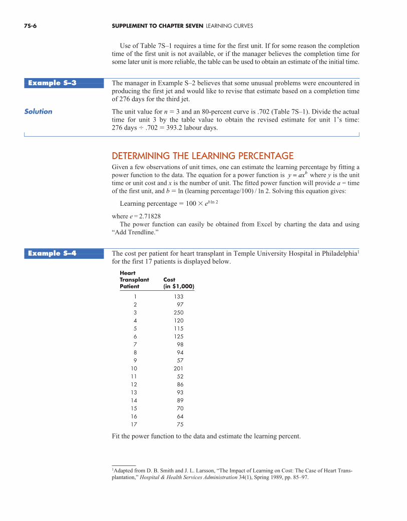
The cost per patient for heart transplant in Temple University Hospital in Philadelphia1

for the first 17 patients is displayed below.

HeartTransplant CostPatient (in $1,000)

1 1332 973 2504 1205 1156 1257 988 949 57

10 20111 5212 8613 9314 8915 7016 6417 75

Fit the power function to the data and estimate the learning percent.

y axb=


Example S–3

Solution

Example S–4

1Adapted from D. B. Smith and J. L. Larsson, “The Impact of Learning on Cost: The Case of Heart Trans-plantation,” Hospital & Health Services Administration 34(1), Spring 1989, pp. 85–97.


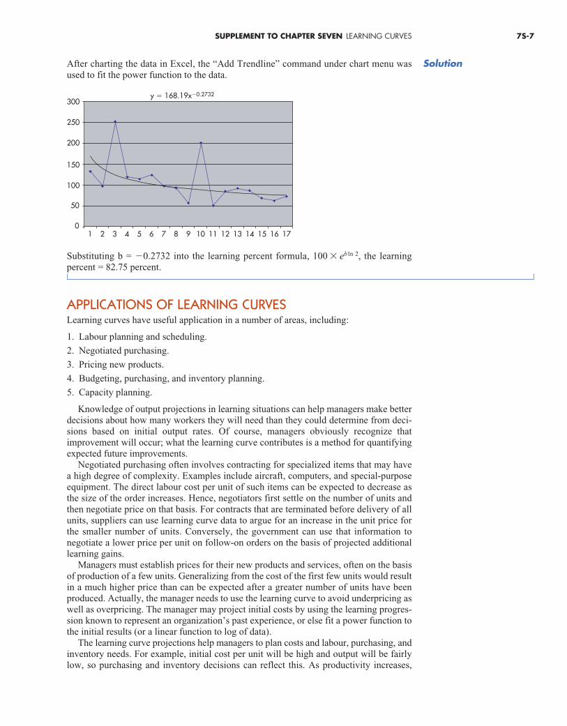
After charting the data in Excel, the “Add Trendline” command under chart menu wasused to fit the power function to the data.

Substituting b = �0.2732 into the learning percent formula, 100 � eb1n 2, the learning percent = 82.75 percent.

APPLICATIONS OF LEARNING CURVESLearning curves have useful application in a number of areas, including:

1. Labour planning and scheduling.

2. Negotiated purchasing.

3. Pricing new products.

4. Budgeting, purchasing, and inventory planning.

5. Capacity planning.

Knowledge of output projections in learning situations can help managers make betterdecisions about how many workers they will need than they could determine from deci-sions based on initial output rates. Of course, managers obviously recognize that improvement will occur; what the learning curve contributes is a method for quantifyingexpected future improvements.

Negotiated purchasing often involves contracting for specialized items that may havea high degree of complexity. Examples include aircraft, computers, and special-purposeequipment. The direct labour cost per unit of such items can be expected to decrease asthe size of the order increases. Hence, negotiators first settle on the number of units andthen negotiate price on that basis. For contracts that are terminated before delivery of allunits, suppliers can use learning curve data to argue for an increase in the unit price forthe smaller number of units. Conversely, the government can use that information to negotiate a lower price per unit on follow-on orders on the basis of projected additionallearning gains.

Managers must establish prices for their new products and services, often on the basisof production of a few units. Generalizing from the cost of the first few units would resultin a much higher price than can be expected after a greater number of units have been produced. Actually, the manager needs to use the learning curve to avoid underpricing aswell as overpricing. The manager may project initial costs by using the learning progres-sion known to represent an organization’s past experience, or else fit a power function tothe initial results (or a linear function to log of data).

The learning curve projections help managers to plan costs and labour, purchasing, andinventory needs. For example, initial cost per unit will be high and output will be fairlylow, so purchasing and inventory decisions can reflect this. As productivity increases,

10

50

100

150

200

250

300

2 3 4 5 6

y � 168.19x�0.2732

7 8 9 10 11 12 13 14 15 16 17


Solution

ste51675_ch07_suppl.qxd 10/11/2006 3:25 PM S-7

purchasing and/or inventory actions must allow for increased usage of raw materials andpurchased parts to keep pace with output. Because of learning effects, the usage rate willincrease over time. Hence, failure to refer to a learning curve would lead to substantialoverestimates of labour needs and underestimates of the rate of material usage.

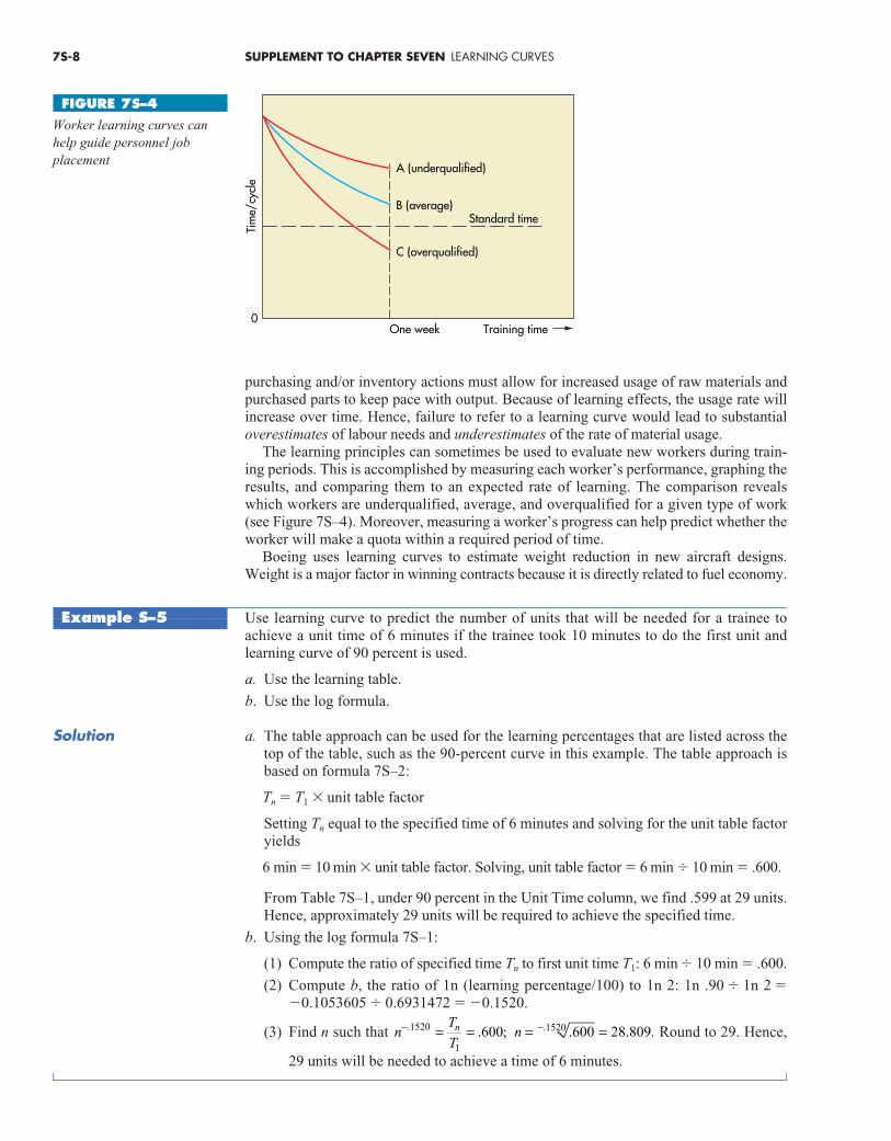
The learning principles can sometimes be used to evaluate new workers during train-ing periods. This is accomplished by measuring each worker’s performance, graphing theresults, and comparing them to an expected rate of learning. The comparison revealswhich workers are underqualified, average, and overqualified for a given type of work(see Figure 7S–4). Moreover, measuring a worker’s progress can help predict whether theworker will make a quota within a required period of time.

Boeing uses learning curves to estimate weight reduction in new aircraft designs.Weight is a major factor in winning contracts because it is directly related to fuel economy.

Use learning curve to predict the number of units that will be needed for a trainee toachieve a unit time of 6 minutes if the trainee took 10 minutes to do the first unit andlearning curve of 90 percent is used.

a. Use the learning table.

b. Use the log formula.

a. The table approach can be used for the learning percentages that are listed across thetop of the table, such as the 90-percent curve in this example. The table approach isbased on formula 7S–2:

Tn � T1 � unit table factor

Setting Tn equal to the specified time of 6 minutes and solving for the unit table factoryields

6 min � 10 min � unit table factor. Solving, unit table factor � 6 min � 10 min � .600.

From Table 7S–1, under 90 percent in the Unit Time column, we find .599 at 29 units.Hence, approximately 29 units will be required to achieve the specified time.

b. Using the log formula 7S–1:

(1) Compute the ratio of specified time Tn to first unit time T1: 6 min � 10 min � .600.

(2) Compute b, the ratio of 1n (learning percentage/100) to 1n 2: 1n .90 � 1n 2 ��0.1053605 � 0.6931472 � �0.1520.

(3) Find n such that Round to 29. Hence,

29 units will be needed to achieve a time of 6 minutes.

nT

Tnn− −= = = =. .. ; . . .1520

1

1520600 600 28 809


Solution

Example S–5

Training time

Tim

e/cy

cle

0One week

A (underqualified)

B (average)

C (overqualified)

Standard time

FIGURE 7S–4

Worker learning curves canhelp guide personnel jobplacement


CAUTIONS AND CRITICISMSManagers using learning curves should be aware of their limitations and pitfalls. This section briefly outlines some of the major cautions and criticisms of learning curves.

1. Learning percentage may differ from organization to organization and by type ofwork. Therefore, it is best to base learning percentage on empirical studies rather thanassumed percentage where possible.

2. Projections based on learning curves should be regarded as approximations of actualtimes and treated accordingly.

3. If time estimates are based on the time for the first unit, considerable care should betaken to ensure that this time is valid. It may be desirable to revise the base time aslater times become available. Since it is often necessary to estimate the time for thefirst unit prior to production, this caution is very important.

4. It is possible that at some point the curve might level off or even tip upward, especiallynear the end of a job. The potential for savings at that point is so slight that most jobsdo not command the attention or interest to sustain improvements. Then, too, some ofthe better workers or other resources may be shifted into new jobs that are starting up.

5. Some of the improvements may be more apparent than real: Improvements in timesmay be caused in part by increases in indirect labour costs.

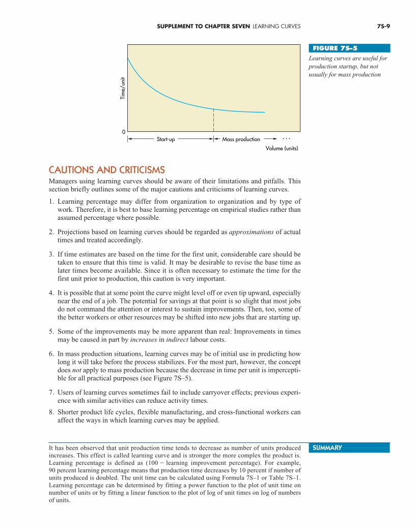
6. In mass production situations, learning curves may be of initial use in predicting howlong it will take before the process stabilizes. For the most part, however, the conceptdoes not apply to mass production because the decrease in time per unit is impercepti-ble for all practical purposes (see Figure 7S–5).

7. Users of learning curves sometimes fail to include carryover effects; previous experi-ence with similar activities can reduce activity times.

8. Shorter product life cycles, flexible manufacturing, and cross-functional workers canaffect the ways in which learning curves may be applied.


Mass production

Tim

e/un

it

0. . .Start-up

Volume (units)

FIGURE 7S–5

Learning curves are useful forproduction startup, but notusually for mass production

SUMMARYIt has been observed that unit production time tends to decrease as number of units produced increases. This effect is called learning curve and is stronger the more complex the product is.Learning percentage is defined as (100 � learning improvement percentage). For example, 90 percent learning percentage means that production time decreases by 10 percent if number ofunits produced is doubled. The unit time can be calculated using Formula 7S–1 or Table 7S–1.Learning percentage can be determined by fitting a power function to the plot of unit time onnumber of units or by fitting a linear function to the plot of log of unit times on log of numbersof units.



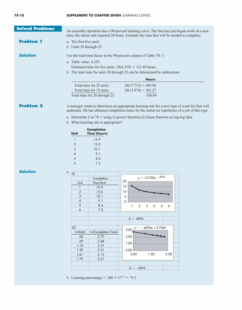
An assembly operation has a 90-percent learning curve. The line has just begun work on a newitem; the initial unit required 28 hours. Estimate the time that will be needed to complete:

a. The first five units.

b. Units 20 through 25.

Use the total time factor in the 90-percent column of Table 7S–1.

a. Table value: 4.339.

Estimated time for five units: 28(4.339) � 121.49 hours.

b. The total time for units 20 through 25 can be determined by subtraction:

Hours

Total time for 25 units: 28(17.713) � 495.96�Total time for 19 units: 28(13.974) � 391.27

Total time for 20 through 25 104.69

A manager wants to determine an appropriate learning rate for a new type of work his firm will undertake. He has obtained completion times for the initial six repetitions of a job of this type.

a. Determine b in 7S–1 using (i) power function (ii) linear function on log-log data.

b. What learning rate is appropriate?

CompletionUnit Time (hours)

1 15.92 12.03 10.14 9.15 8.46 7.5

a.

b. Learning percentage � 100 � eb1n 2 � 75.3

Solved Problems

Problem 1

Solution

Problem 2

Solution (i)Completion

Unit Time (hrs)123456

15.912.010.1

9.18.47.5

b � .4094

(ii)1n (Completion Time)1n (Unit)

.00 2.77

.69 2.481.10 2.311.39 2.211.61 2.131.79 2.01

b ��.4094

y � 15.928x �.4094

0

510

15

20

1 2 3 4 5 6

y � �.4094x + 2.7681

0.00

1.00

2.00

3.00

0.00 1.00 2.00


1. If the learning phenomenon applies to all human activity, why isn’t the effect noticeable inmass production or high-volume assembly work?

2. Under what circumstances is most learning possible?

3. What would a learning percentage of 80 percent imply?

4. Explain how an increase in indirect labour cost can contribute to a decrease in direct labourcost per unit.

5. List the kinds of factors that create the learning effect.

6. Explain how changes in a process, once it is under way, can cause scallops in a learning curve.

7. Name some areas in which learning curves are useful.

8. What factors might cause a learning curve to tip up toward the end of a job?

9. Users of learning curves sometimes fail to include carryover effects. What is meant by this?

Verify the values in Table 7S–1 using the learning curve calculator in www.jsc.nasa.gov/bu2/learn.html. Choose Crawford’s method.

1. An aircraft services company has an order to refurbish the electronics of 18 jet aircraft. Thework has a learning curve percentage of 80 percent. On the basis of experience with similarjobs, the industrial engineering department estimates that the first plane will require 300 hoursto refurbish. Estimate the amount of time needed to complete:

a. The fifth plane.

b. The first five planes.

c. All 18 planes.

2. Estimate the time it will take to complete the 4th unit of a 12-unit job involving a large assem-bly if the initial unit required approximately 80 hours for each of these learning percentages:

a. 72 percent

b. 87 percent

c. 95 percent

3. A small contractor intends to bid on a job installing 30 in-ground swimming pools. Becausethis will be a new line of work for the contractor, he believes there will be a learning effect forthe job. After reviewing time records from a similar type of activity, the contractor is con-vinced that an 85-percent curve is appropriate. He estimates that the first pool will take hiscrew eight days to install. How many days should the contractor budget for:

a. The first 10 pools?

b. The second 10 pools?

c. The final 10 pools?

4. A job is known to have a learning percentage equal to 82. If the first unit had a completiontime of 20 hours, estimate the times that will be needed to complete the third and fourth units.

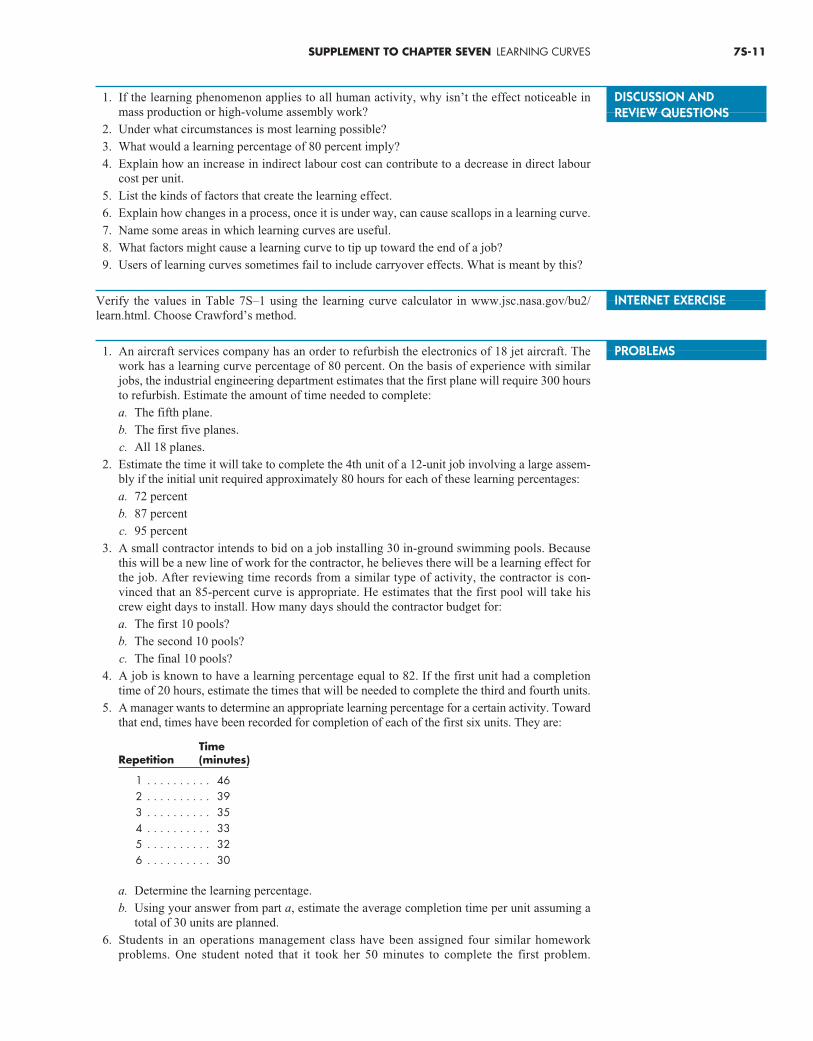
5. A manager wants to determine an appropriate learning percentage for a certain activity. Towardthat end, times have been recorded for completion of each of the first six units. They are:

TimeRepetition (minutes)

1 . . . . . . . . . . 462 . . . . . . . . . . 393 . . . . . . . . . . 354 . . . . . . . . . . 335 . . . . . . . . . . 326 . . . . . . . . . . 30

a. Determine the learning percentage.

b. Using your answer from part a, estimate the average completion time per unit assuming atotal of 30 units are planned.

6. Students in an operations management class have been assigned four similar homeworkproblems. One student noted that it took her 50 minutes to complete the first problem.


DISCUSSION AND REVIEW QUESTIONS

PROBLEMS

INTERNET EXERCISE


Assume that the four problems are similar and that a 70-percent learning curve is appropriate.How much total time can this student plan to spend solving the remaining problems?

7. A subcontractor is responsible for outfitting six satellites that will be used for solar research.Four of the six have been completed in a total of 600 hours. If the crew has a 75-percent learn-ing curve, how long should it take them to finish the last two units?

8. The 5th unit of a 25-unit job took 14.5 hours to complete. If a 90-percent learning curve is appropriate:

a. How long should it take to complete the last unit?

b. How long should it take to complete the 10th unit?

c. Estimate the average time per unit for the 25 units.

9. The labour cost to produce a certain item is $8.50 per hour. Job setup costs $50 and material costsare $20 per unit. The item can be purchased for $88.50 per unit. The learning percentage is 90 percent. Overhead is charged at a rate of 50 percent of labour, materials, andsetup costs. Determine the unit cost for 20 units, given that the first unit took 5 hours to complete.

10. A firm has a training program for a certain operation. The progress of trainees is carefully mon-itored. An established standard requires a trainee to be able to complete the sixth repetition ofthe operation in six hours or less. Those who are unable to do this are assigned to other jobs.

Currently, three trainees have each completed two repetitions. Trainee A had times of 9 hours for the first and 8 hours for the second repetition; trainee B had times of 10 hours and8 hours for the first and second repetitions; and trainee C had times of 12 and 9 hours.

Which trainee(s) do you think will make the standard? Explain your reasoning.

11. The first unit of a job took 40 hours to complete. The work has a learning percentage of 88.The manager wants time estimates for units 2, 3, 4, and 5. Develop those time estimates.

12. A manager wants to estimate the remaining time that will be needed to complete a five-unitjob. The initial unit of the job required 12 hours, and the work has a learning percentage of 77.Estimate the total time remaining to complete the job.

13. A job is supposed to have a learning percentage of 82. Times for the first four units were 30.5,28.4, 27.2, and 27.0 minutes. Does a learning percentage of 82 seem reasonable? Fit a powerfunction to data.

14. The 5th unit of a 10-unit job took five hours to complete. The 6th unit has been worked on fortwo hours, but is not yet finished. Estimate the additional amount of time needed to finish the10-unit job if the work has a 75-percent learning percentage.

15. Estimate the number of repetitions each of the workers listed in the table below will require toreach a time of 7 hours per unit. Time is in hours.

Trainee T1 T2

Art 11 9.9Sherry 10.5 8.4Dave 12 10.2

16. Estimate the number of repetitions that new service worker Irene will require to achieve “stan-dard” if the standard is 18 minutes per repetition. She took 30 minutes to do the initial repeti-tion and 25 minutes to do the next repetition.

17. Estimate the number of repetitions each of the workers listed in the following table will requireto achieve a standard time of 25 minutes per repetition. Time is in minutes.

Trainee T1 T2

Tracy 36 31Darren 40 36Lynn 37 30

18. A research analyst performs database searches for a variety of clients. According to her log, anew search requires approximately 55 minutes. Repeated requests on the same or similar topictake less and less time, as her log shows:

Request no. 1 2 3 4 5 6 7 8Time (min.) 55.0 41.0 35.2 31.0 28.7 26.1 24.8 23.5

How many more searches will it take until the search time gets down to 19 minutes?



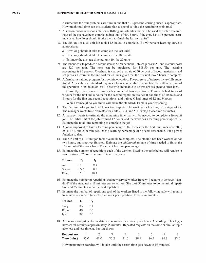
19. The following data are the hours it took to assemble 20 identical sections of an aircraftfuselage.2 Use Excel to fit a power function to it and determine the learning percentage.

Units ActualProduced Unit Time

1 21222 15123 12834 8485 7556 7987 6978 8259 759

10 79811 78812 77113 77414 77015 77816 78617 77718 78519 78120 764

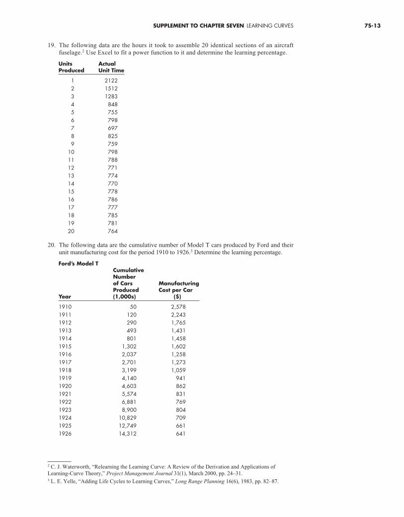
20. The following data are the cumulative number of Model T cars produced by Ford and theirunit manufacturing cost for the period 1910 to 1926.3 Determine the learning percentage.

Ford’s Model TCumulative Numberof Cars ManufacturingProduced Cost per Car

Year (1,000s) ($)

1910 50 2,5781911 120 2,2431912 290 1,7651913 493 1,4311914 801 1,4581915 1,302 1,6021916 2,037 1,2581917 2,701 1,2731918 3,199 1,0591919 4,140 9411920 4,603 8621921 5,574 8311922 6,881 7691923 8,900 8041924 10,829 7091925 12,749 6611926 14,312 641


2 C. J. Waterworth, “Relearning the Learning Curve: A Review of the Derivation and Applications of Learning-Curve Theory,” Project Management Journal 31(1), March 2000, pp. 24–31.3 L. E. Yelle, “Adding Life Cycles to Learning Curves,” Long Range Planning 16(6), 1983, pp. 82–87.



An automobile manufacturer is conducting a product recallafter it was discovered that a possible defect in the steer-

ing mechanism could cause loss of control in certain cars. Therecall covers a span of three model years. The company sentout letters to car owners promising to repair the defect at nocost at any dealership.

The company’s policy is to pay the dealer a fixed amountfor each repair. The repair is somewhat complicated, and thecompany expects learning to be a factor. In order to set a reasonable rate for repairs, company engineers conducted anumber of repairs themselves. It was then decided that a rateof $88 per repair would be appropriate, based on a flat hourlyrate of $22 per hour and 90-percent learning.

Shortly after dealers began making repairs, the company received word that several dealers were encountering resistance

from workers who felt the flat rate was much too low and whowere threatening to refuse to work on those jobs. One of thedealers collected data on job times and sent that information tothe company: three mechanics each completed two repairs.Average time for the first unit was 9.6 hours, and average timefor the second unit was 7.2 hours. The dealer has suggested arate of $110 per repair.

You have been asked to investigate the situation and toprepare a report.

Questions

1. Prepare a list of questions that you will need to have answered in order to analyze this situation.

2. Comment on the information provided in the case.

3. What preliminary thoughts do you have on solutions/partialsolutions to the points you have raised?

M I N I - C A S E

Product Recall

N ew surgery techniques require a long learning curve onthe part of a general surgeon. Random complications

may arise due to patients’ conditions. Therefore, it is importantto know the number of operations required to stabilize operat-ing times and complication rates.

Dr. Voitk of Salvation Army Scarborough Grace Hospitalreported the results of 100 consecutive operations for laparo-scopic hernia repair on 98 patients between March 1992 andMay 1996. Approximately two-thirds of surgeries were uni-lateral (right/left) and the remaining one-third were bilateral(involving contralateral defects; many unsuspected beforesurgery). The average surgery time (from skin incision toskin closure) was 46 minutes for unilateral and 62 minutesfor bilateral. Surgery times for the unilateral procedure beganto level off after 50 operations. Dr. Voitk reported the average surgery times (in minutes) for each quartile of the100 operations, classified by type of operation, as follows:

1st Quartile 2nd Quartile 3rd Quartile 4th Quartile

Unilateral 59 45 38 37Bilateral 69 67 58 52

At the end of the study the times had levelled off at 58 minutes(operating time), and 37 minutes (surgical time) for unilateraltype, which approached the historical times for open repair.Learning also reduced the complication rates, which fell in anapproximately exponential manner, beginning to level off at50 operations and becoming stable after 75.

Questions

1. Determine the learning percentage for the unilateral laparo-scopic hernia surgery. (Hint: Use 2/3 of the midpoint observation of each of the four quartiles as having the unilateral surgery times; that is, assume that the 19th, 25th,42nd, and 59th observations had the unilateral surgerytimes.)

2. Determine the learning percentage for the bilateral laparo-scopic hernia surgery. (Hint: Use 1/3 of the midpoint observation of each of the four quartiles, i.e., the 4th, 13th,21st, and 29th observations). Compare your answers.

Source: Adapted from Dr. Andrus Voitk, “The Learning Curve in Laparoscopic Inguinal Hernia Repair for the Community GeneralSurgeon,” Canadian Journal of Surgery 41(6) December 1998, pp. 446–450.

M I N I - C A S E

Learning Curve inSurgery



T en sections completed, 44 more to go. The repairs are con-troversial, behind schedule, over budget, and subject to

penalties. American Bridge/Surespan staff is contemplatinghow long it will take to install the remaining sections of LionsGate Bridge.

Lions Gate Bridge, the scenic entranceway to Vancouver’sBurrard Inlet, began service in 1938. At that time, its twolanes of traffic appeared more than ample. By the 1950s how-ever, commuters to and from Vancouver’s north shore werecausing rush-hour line-ups. In 1952 two lanes were convertedto three narrow lanes. But continued expansion on the northshore, growth of the Whistler ski community, and increasedferry service to Vancouver Island caused the bridge to reachits capacity.

Over the years, Lions Gate Bridge had undergone regularmaintenance. Although its suspension cables and steel super-structure have never been changed, the bridge has undergoneperiodic painting and re-surfacing. On the viaduct section inthe north, the cantilevering of sidewalks allowed increasedlane widths and separation of pedestrians from traffic. This accentuated the need for change on the rest of the bridge.

By the 1990s, the annual cost of maintenance made the existing situation uneconomical. The bridge either had to be repaired to “good as new” or an alternate crossing had to bebuilt. The debate became extreme. Some proposed doublingcapacity with a twin bridge or a new four-lane bridge. Other

plans included various locations for a tunnel or combinationsof bridges and tunnels. At the same time, the Parks Board andenvironmentalists opposed cutting of trees or any encroach-ment on Stanley Park. Consensus seemed impossible.

Complicating the issue was money. Highway constructionis a provincial responsibility, but deficit financing alreadyoverwhelmed the government. User tolls were a possibility,but north shore communities claimed that tolls would be discrimination when not applied to other bridges. Private ownership, while a possibility, suffered from criticisms of tollsand monopoly. In the end, money ruled. In May 1999, theprovincial government chose to replace only the deck of theexisting bridge.

The outcry was instantaneous. While the bridge would bemade safer, the same capacity problems would remain. Publicmeetings were held, citizens signed petitions, and “stop work”injunctions were sought through the court system. When temperscooled, a detailed news article looked back and pronounced “Lions Gate Renewal Defies Reason.”4

A team headed by American Bridge (AB) of Pittsburghwas selected to rehabilitate the bridge. In order to carry outthe work, they assembled a group of other professionals forconstruction design.

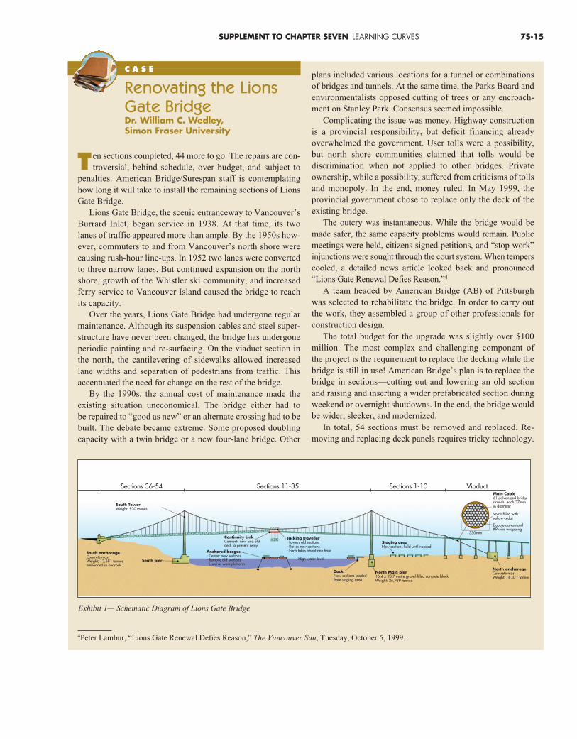
The total budget for the upgrade was slightly over $100million. The most complex and challenging component of the project is the requirement to replace the decking while thebridge is still in use! American Bridge’s plan is to replace thebridge in sections—cutting out and lowering an old sectionand raising and inserting a wider prefabricated section duringweekend or overnight shutdowns. In the end, the bridge wouldbe wider, sleeker, and modernized.

In total, 54 sections must be removed and replaced. Re-moving and replacing deck panels requires tricky technology.

C A S E

Renovating the LionsGate BridgeDr. William C. Wedley, Simon Fraser University

South TowerWeight: 930 tonnes

Continuity LinkConnects new and olddeck to prevent sway

Jacking traveller- Lowers old sections- Raises new sections- Each takes about one hour

DockNew sections loadedfrom staging area

North anchorageConcrete massWeight: 18,371 tonnes

North Main pier16.4 × 25.7 metre gravel-filled concrete blockWeight: 26,989 tonnes

Staging areaNew sections held until needed

Anchored barges- Deliver new sections- Remove old sections- Used as work platform

South anchorageConcrete massWeight; 13,681 tonnesembedded in bedrock

South pier High water level

Main Cable

Voids filled withyellow cedar

Double galvanized#9 wire wrapping

Sections 36-54 Sections 11-35 Sections 1-10 Viaduct

Exhibit 1— Schematic Diagram of Lions Gate Bridge

4Peter Lambur, “Lions Gate Renewal Defies Reason,” The Vancouver Sun, Tuesday, October 5, 1999.



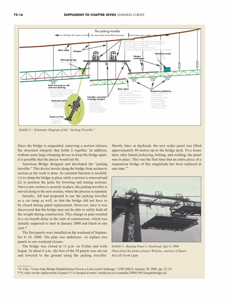
Rails mounted on oldand new decking

To move the traveller to the nextsection its legs are extendedallowing small tracks on its feet toengage the rails

Hydraulic jacksAdjust the heightof the traveller’stelescoping legs

Tracks on feetRun in railsinstalled onbridge deck

Traveller connectedto bridge hangers

The traveller issupported byconnecting it tothe bridge hangersbefore the old bridgesection is removed

Deck splice- Deck sections are attached or“spliced” together

- Each splice uses 800 boltsranging from three quarters ofan inch to one inch indiameter and from one-and-a-half to four inches long

Temporary platforms- Specially constructedfor the project

- Run on tracks underthe bridge deck

- First is for boltingsections together

- Second for welding- Third for painting

Strand jacks- Hydraulic jacks are used instead of winches becausethe pump which powers them can be at a distancereducing weight on the traveller

- Each of the four jacks can lift 30 tonnes- The jacks will take about an hour to lower or lift each section

Old deck still in place New deck section being lifted into position New deck installed

The jacking traveller

Main cable Hangers

Telescoping legs(See close-up below)

Hangerextensions

Hydraulic pump- Powers furstrand jacks

Exhibit 2— Schematic Diagram of the “Jacking Traveller”

Since the bridge is suspended, removing a section releasesthe structural integrity that holds it together. In addition,without some large clamping device to keep the bridge apart,it is possible that the pieces would not fit.

American Bridge designed and developed the “jackingtraveller.” This device travels along the bridge from section tosection as the work is done. Its essential function is twofold:(1) to clamp the bridge in place while a section is removed and(2) to position the jacks for lowering and raising sections.Once a new section is securely in place, the jacking traveller ismoved along to the next section, where the process is repeated.

Initially, AB had proposed to use the jacking traveller as a car ramp as well, so that the bridge did not have to be closed during panel replacement. However, later it was discovered that the bridge may not be able to safely hold allthe weight during construction. This change in plan resultedin a six-month delay in the start of construction, which wasinitially supposed to start in January 2000 and finish in oneyear.*

The first panels were installed on the weekend of Septem-ber 8–10, 2000. The plan was ambitious—to replace twopanels in one weekend closure.

The bridge was closed at 11 p.m. on Friday and work began. At about 6 a.m., the first of the 54 panels was cut outand lowered to the ground using the jacking traveller.

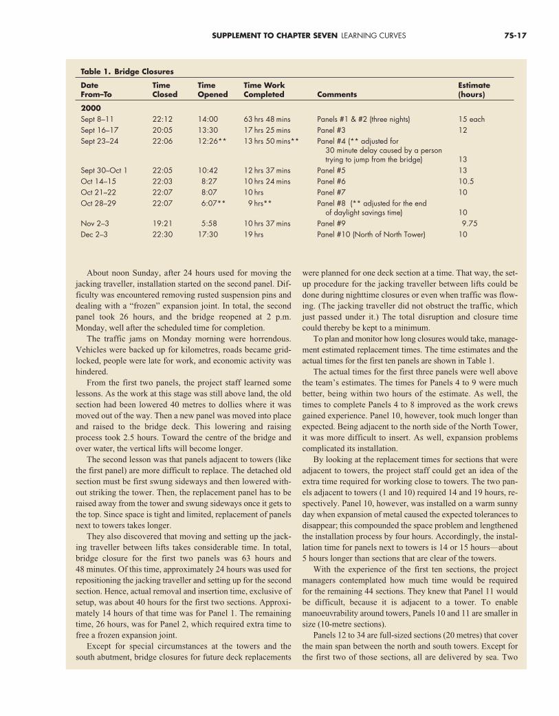
Shortly later, at daybreak, the new wider panel was lifted approximately 40 metres up to the bridge deck. Five hourslater, after lateral jockeying, bolting, and welding, the panelwas in place. This was the first time that an entire piece of asuspension bridge of this magnitude has been replaced atone time.**

Exhibit 3—Raising Panel 1, Daybreak, Sept 9, 2000

Photo from the former project Website, courtesy of Stuart

McCall/North Light

*A. Cho, “Lions Gate Bridge Rehabilitation Proves a Lion-sized Challenge,” ENR 248(3), January 28, 2002, pp. 22–25.**A video on the replacement of panel # 5 is located at mms://media.tsn.ca/exnmedia/20001109-liongatebridge.asf.



About noon Sunday, after 24 hours used for moving thejacking traveller, installation started on the second panel. Dif-ficulty was encountered removing rusted suspension pins anddealing with a “frozen” expansion joint. In total, the secondpanel took 26 hours, and the bridge reopened at 2 p.m. Monday, well after the scheduled time for completion.

The traffic jams on Monday morning were horrendous. Vehicles were backed up for kilometres, roads became grid-locked, people were late for work, and economic activity washindered.

From the first two panels, the project staff learned somelessons. As the work at this stage was still above land, the oldsection had been lowered 40 metres to dollies where it wasmoved out of the way. Then a new panel was moved into placeand raised to the bridge deck. This lowering and raisingprocess took 2.5 hours. Toward the centre of the bridge andover water, the vertical lifts will become longer.

The second lesson was that panels adjacent to towers (likethe first panel) are more difficult to replace. The detached oldsection must be first swung sideways and then lowered with-out striking the tower. Then, the replacement panel has to beraised away from the tower and swung sideways once it gets tothe top. Since space is tight and limited, replacement of panelsnext to towers takes longer.

They also discovered that moving and setting up the jack-ing traveller between lifts takes considerable time. In total,bridge closure for the first two panels was 63 hours and 48 minutes. Of this time, approximately 24 hours was used forrepositioning the jacking traveller and setting up for the secondsection. Hence, actual removal and insertion time, exclusive ofsetup, was about 40 hours for the first two sections. Approxi-mately 14 hours of that time was for Panel 1. The remainingtime, 26 hours, was for Panel 2, which required extra time tofree a frozen expansion joint.

Except for special circumstances at the towers and thesouth abutment, bridge closures for future deck replacements

were planned for one deck section at a time. That way, the set-up procedure for the jacking traveller between lifts could bedone during nighttime closures or even when traffic was flow-ing. (The jacking traveller did not obstruct the traffic, whichjust passed under it.) The total disruption and closure timecould thereby be kept to a minimum.

To plan and monitor how long closures would take, manage-ment estimated replacement times. The time estimates and theactual times for the first ten panels are shown in Table 1.

The actual times for the first three panels were well abovethe team’s estimates. The times for Panels 4 to 9 were muchbetter, being within two hours of the estimate. As well, thetimes to complete Panels 4 to 8 improved as the work crewsgained experience. Panel 10, however, took much longer thanexpected. Being adjacent to the north side of the North Tower,it was more difficult to insert. As well, expansion problemscomplicated its installation.

By looking at the replacement times for sections that wereadjacent to towers, the project staff could get an idea of the extra time required for working close to towers. The two pan-els adjacent to towers (1 and 10) required 14 and 19 hours, re-spectively. Panel 10, however, was installed on a warm sunnyday when expansion of metal caused the expected tolerances todisappear; this compounded the space problem and lengthenedthe installation process by four hours. Accordingly, the instal-lation time for panels next to towers is 14 or 15 hours—about5 hours longer than sections that are clear of the towers.

With the experience of the first ten sections, the projectmanagers contemplated how much time would be required for the remaining 44 sections. They knew that Panel 11 wouldbe difficult, because it is adjacent to a tower. To enable manoeuvrability around towers, Panels 10 and 11 are smaller insize (10-metre sections).

Panels 12 to 34 are full-sized sections (20 metres) that coverthe main span between the north and south towers. Except forthe first two of those sections, all are delivered by sea. Two

Table 1. Bridge Closures

Date Time Time Time Work Estimate From–To Closed Opened Completed Comments (hours)

2000 Sept 8–11 22:12 14:00 63 hrs 48 mins Panels #1 & #2 (three nights) 15 eachSept 16–17 20:05 13:30 17 hrs 25 mins Panel #3 12Sept 23–24 22:06 12:26** 13 hrs 50 mins** Panel #4 (** adjusted for

30 minute delay caused by a persontrying to jump from the bridge) 13

Sept 30–Oct 1 22:05 10:42 12 hrs 37 mins Panel #5 13Oct 14–15 22:03 8:27 10 hrs 24 mins Panel #6 10.5Oct 21–22 22:07 8:07 10 hrs Panel #7 10Oct 28–29 22:07 6:07** 9 hrs** Panel #8 (** adjusted for the end

of daylight savings time) 10Nov 2–3 19:21 5:58 10 hrs 37 mins Panel #9 9.75Dec 2–3 22:30 17:30 19 hrs Panel #10 (North of North Tower) 10



barges with accompanying tugboats jockey into place belowthe opening, one to receive the old section and the other to deliver the new panel. The required vertical lift from the bargesdepends upon the tides at the time of the lift. The typical liftfrom the water level is expected to be 55 metres, as opposed to40 metres over land. The increased distance and the jockeyingof barges are expected to increase the removal and lifting timeby one hour (i.e., 3.5 hours over water vs. 2.5 hours over land).

After Panel 34, the size changes to 10 metres but with nochange in the lifting, bolting, and welding times. Panels 35 and36, next to the south tower, are expected to take longer. Panels37 and 38 are spliced together beforehand, delivered on a narrow barge at high tide, and lifted and installed as one piece.This splicing to form a double panel avoids one bridge closure,but the horizontal jockeying of a larger section adds about twohours to the replacement.

Panels 39 to 53 are installed differently. Since the land belowis steep cliff, delivery and installation is done from above. First,the 10-metre section cut from the bridge is raised above the decklevel and turned 90 degrees. A truck with extended girders backsonto the bridge from the south end so that its girders extend overthe gap. The old section is then lowered onto the girders, movedonto the truck, and driven away. In the meantime, the new section is backed over the entire bridge from the north end on a similar truck. The new section is raised from the truck’s girders,rotated 90 degrees, and lowered into the opening after the truckis removed. Although this process does not require as much timejacking sections up and down, it requires the tricky 90-degreeturn. In this regard, Panels 39 to 53 are new learning experiences.

The final panel, number 54, is unique. Unlike Panels 39 to53, it is longer (12 metres) and requires a different installationprocedure. Being longer, it cannot be backed over the bridge orswung 90 degrees before installation. As a result, both removal

of the old section and delivery of the new panel are done fromthe south abutment.

As a consequence of engineering delays and adverseweather conditions in December and January, the replacementschedule was cancelled for those months. This provided a timefor reflection for the project managers. Given their experienceto date, they had to estimate how long each remaining sectionwould take for removal and replacement. With those estimates,they would be able to determine a closure schedule that wouldminimize disruption to the community, but ensure safety forworkers and the public.

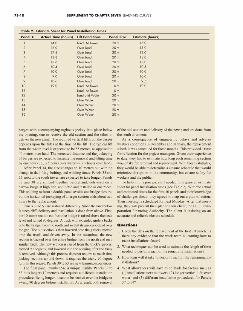
To help in this process, staff needed to prepare an estimatesheet for panel installation times (see Table 2). With the actualand estimated times for the first 10 panels and their knowledgeof challenges ahead, they agreed to map out a plan of action.Their meeting is scheduled for next Monday. After that meet-ing, they will present their plan to their client, the B.C. Trans-portation Financing Authority. The client is insisting on anaccurate and reliable closure schedule.

Questions

1. Given the data on the replacement of the first 10 panels, isthere any evidence that the work team is learning how tomake installations faster?

2. What techniques can be used to estimate the length of timeneeded to perform each of the remaining installations?

3. How long will it take to perform each of the remaining in-stallations?

4. What allowances will have to be made for factors such as(1) installations next to towers, (2) longer vertical lifts overwater, and (3) different installation procedures for Panels37 to 54?

Table 2. Estimate Sheet for Panel Installation Times

Panel # Actual Time (hours) Lift Conditions Panel Size Estimate (hours)

1 14.0 Land, At Tower 20 m 15.02 26.0 Over Land 20 m 15.03 17.4 Over Land 20 m 12.04 13.8 Over Land 20 m 13.05 12.6 Over Land 20 m 13.06 10.4 Over Land 20 m 10.57 10.0 Over Land 20 m 10.08 9.0 Over Land 20 m 10.09 10.6 Over Land 20 m 9.75

10 19.0 Land, At Tower 10 m 10.011 Land, At Tower 10 m12 Land and Water 20 m13 Over Water 20 m14 Over Water 20 m15 Over Water 20 m16 Over Water 20 m



SELECTEDBIBLIOGRAPHY ANDFURTHER READING

Abernathy, W. J. “The Limits of the Learning Curve.” Harvard Business Review, September–October 1974,pp. 109–19.

Argote, Linda, and Dennis Epple. “Learning Curves in Manufacturing.” Science 247, February 1990, pp. 920–24.

Belkauoi, Ahmed. The Learning Curve. Westport, CT:Greenwood Publishing Group, 1986.

Fabrycky, W. J., P. M. Ghare, and P. E. Torgersen. IndustrialOperations Research. Englewood Cliffs, NJ: PrenticeHall, 1972.

Teplitz, Charles J. The Lear.


learning curve supplement_ch07.pdf

Documents

learning effect

learning percentage

learning curve insurgery

actual worker learning

number of changes

routine activities

onlearning curves

concept of alearning