NBER WORKING PAPER SERIES

A TRANSACTIONS BASED MODEL OF THE MONETARYTRANSMISSION MECHANISM: PART 1

Sanford J. Grossman

Laurence Weiss

Working Paper No. 973

NATIONAL BUREAU OF ECONOMIC RESEARCH1050 Massachusetts Avenue

Cambridge MA 02138

September 1982

The research reported here is part of the NBER's research programsin Economic Fluctuations and in Financial Markets and Monetary

Economics. Any opinions expressed are those of the authors and notthose of the National Bureau of Economic Research.

NBER Working Paper //973

September 1982

A Transactions Based Model of the Monetary

Transmission Mechanism: Part I

ABSTRACT

What are the effects of open market operations? How do these differ

from money falling from heaven? We propose a new explanation of how open

market operations can change real and nominal interest rates which emphasizes

three often mentioned but seldom explicitly articulated features of actual

monetary economies: i) going to the bank is costly so that people will tend to

bunch cash withdrawals, ii) people don't all go to the bank simultaneously and,

because of these, iii) at any instant of time agents hold different amounts of

cash. We show that these considerations imply that an open market purchase

of a bond for fiat money will drive down nominal and real interest rates, lead

to a delayed positive price response, and have damped persistent effects on

both prices and nominal interest rates if agents have logarithmic utility of

consumption. We assume output is exogenous, so that the model can shed only

indirect light on the relationship between money and aggregate output.

The model has emphasized how a change in the money supply affects the

spending decision of those agents making withdrawals at the time of an open

market operation. Considerations of intertemporal substitution imply that

the real rate must decline to induce these agents to consume more. Because

this new money is spent gradually, prices will rise slowly and reach their

steady state level long after the interval of time between trips to the bank.

Professor Sanford GrossmanProfessor Laurence WeissUniversity of ChicagoDepartment of Economics1126 E. 59th StreetChicago, Illinois 60637

(312)962—8178

July 1982

A Transactions Based Model of the Monetary

Transmission Mechanism: Part I

by

*Sanford Grossman and Laurence Weiss

I. Introduction

What are the effects of open market operations? How do these differ

from money falling from heaven? We propose a new explanation of how open

market operations can change real and nominal interest rates which emphasizes

three often mentioned but seldom explicitly articulated features of actual

monetary economies 1) going to the bank is costly so that people will tend to

bunch cash withdrawals ii) people don't all go to the bank simultaneously and,

because of these iii) at any instant of time agents hold differentainounts

of cash. We show that these considerations imply that an open market purchase

of a bond for fiat money will drive down nominal and real interest rates, lead

to a delayed positive price response, and have damped persistent effects on both

prices and nominal interest rates if agents have logarithmic utility of consumption.

We assume output is exogenous, so that the model can shed only indirect light on

the relationship between money and aggregate output.

The model is a hybrid of the type suggested by Clower (1967) which assumes

that agents require cash in advance of expenditures, and the partial equilibrium

inventory theoretic models of Tobin (1956) and Baumol (1952) which stress that

transaction costs necessitate that money withdrawals be periodic, so that it

will not be optimal for agents to go to the bank at each instant.

*Research supported by NSF grant SES—8112036.

2

Formally, we assume that money withdrawals are staggered, so that a fixed

fraction of the population makes a withdrawal each period. While it would

certainly be preferable to make the time between trips to the bank an endogenous

choice variable as in the Tobin—Baumol model, analysis of this consideration

outside of steady states is too complicated, so that we choose this simpler

formulation. (See Jovanovic (1982) for the analysis of the steady state time

between trips to the bank in a model similar in structure to ours). As we hope

will be clear, letting the time between trips to the bank adjust to changes

brought about by open market operations would not substantially alter our

conclusion regarding the non—neutrality of money.

Although the timing of withdrawals is fixed, the size of these

withdrawals is endogenously determined. All income receipts are assumed to

accrue as interest earning deposits, so that bank withdrawals are the only

source of cash for consumers. The Clower cash—inadvance constraint implies

that withdrawals for each agent equal his planned nominal spending over the

ensuing time interval before his next withdrawal. Planned nominal spending

is determined by the possibility of intertemporal consumption substitution and

thus is influenced by expected prices and future nominal interest rates. The

model is completely deterministic and we assume that those expectations are in

fact realized; we attribute to agents perfect foresight.

We assume that only consumers hold stocks of fiat money. The consumers

use money to buy goods from firms. We assume that firms deposit their cash

receipts instantly into the interest bearing accounts of their various claimants

and hold no money themselves. Similarly, under certainty it is difficult

to see why banks would hold cash at positive interest rates; we assume they

hold none. Under this formulation the money stock is held exclusively by

3

consumers to finance spending before their next withdrawal. Equilibrium

requires that the flow of cash into the bank at each period equal agents'

desired withdrawals. The flow into the bank consists of the nominal value

of firms' receipts (nominal GNP) plus any changes in nominal money introduced

by open market operations.

An essential feature of our model is the fact that it is optimal for

people to take time to run down their cash balances. Thus if there is to

be a steady flow of money out of the bank, there will have to be a steady

rate at which people run out of money. Thus the cross sectional distribution

of money holdings at a given point in time cannot be degenerate. If everyone

holds exactly the same amount of money then they will exhaust at the same

day. On the dates when they don't exhaust there would beno one to hold the

(non interest) bearing money which flows from the stores to the banks. Thus

it is impossible to have everyone exhaust at the same time.

Under this formulation it is straightforward to see how an open market

purchase differs from a transfer to each agent proportional to his existing

nominal balances. When the money supply increases through an open market

operation agents at the bank must be induced to hold the whole of the increase

and thus a disproportionately larger share of the stock of money. This is

because most of the people who are not at the bank (i.e., those people who

have not yet exhausted their cash balances) will not find it optimal to go

to the bank and withdraw extra cash, until they exhaust their current cash.

Thus, the share of nominal spending attributable to agents at the bank must

rise. To induce agents at the bank to withdraw and hence consume more, banks

must lower the real and nominal interest rates. Since this new money is

4

spent gradually over the interval before the next trip to the bank, the price

level rises gradually through time, even though prices are completely flexible.

This scenario contrasts with a proportional transfer which would raise all

nominal prices by the same percentage and thus have no real effects.

The types of wealth redistribution associated with open market operations

are novel features of the analysis. We emphasize that the new money withdrawal

is financed by running down other asset holdings of equal nominal value; there

is no direct benefit bestowed on the recipients of the new money. Rather,

wealth is redistributed through two indirect channels. The first channel involves

the asymmetry of existing nominal holdings of money. Since those agents not

currently at the bank have more money than those at the bank (who have none),

the inflation induced by money creation redistributes wealth from those not

at the bank to those at the bank. The second channel is more subtle and

focus on the redistribution arising from interest rate changes. We assume

that all current period receipts accrue as interest earning deposits. Thus

those agents not at the bank implicitly lend their current period income to

those making withdrawals. A decline in interest rates redistributes wealth

from creditors to debtors, which enhances the relative position of those making

withdrawals when interest rates decline as a result of open market purchases.

The paper is organized as follows: Section 2 outlines the model. Section 3

discusses the properties of the steady state equilibrium. Section 4 considers

the effects of both a one time proportional transfer and of an open market -

operation for the case of logarithmic utility. This assumption simplifies the

analyéis by making consumption independent of the real interest rate. (In

Part 2, the results are extended to the case where future consumption is an incréasing

function of the real interest rate). The Fifth section presents conclusions

and relates our model to other models. The Appendix outlines a continuous time

version of our model.

5

2. Model

2A. The Flow of Money

We assume that there is a market where interest earning assets

can be bought and sold in exchange for money (a noninterest bearing asset).

We call this market a bank and assume that there is a fixed transaction cost

of "going to the bank", i.e. of converting an interest bearing asset into

money. We assume that there is another market, called "stores", where

consumers buy goods with money. Goods can only be bought with money.

Given the fixed transactions cost of going to the bank, consumers

will not find it optimal to go to the bank for each transaction. Instead

they will go to the bank occasionally and withdraw a stock of money which

they then use up over time by purchasing goods. We assume that consumers'

expenditures and receipts are not perfectly synchronized. In order to

generate a non—degenerate cross—sectional distribution of money holdings we

want the nonsyncronization to imply that it is optimal for a consumer to have

a stock of money which is a declining function of the length of time since

his last trip to the bank. This characteristic is most easily developed

in a model where all of the consumer's receipts arrive at the bank, so that

the only source of cash consumers have is via withdrawals from the bank.

Since the "bank" is a shorthand for an asset market it makes no

sense to imagine that the "bank" holds a stock of money when the nominal

interest rate is positive. If some consumers are making withdrawals from

the bank, then other consumers must be making deposits which exactly equal

the withdrawals. We assume that the flow of money into the bank is being

6

generated by the expenditures of consumers at the stores, and the stores

instantaneously deposit their receipts at the bank. More precisely, we

consider an economy where output is exogenous and consumers own the stores

which own the economy's endowment of goods. As money comes into the stores,

the stores deposit the money in consumers' bank accounts (i.e. they purchase

interest bearing securities for their owners).

In the above description of the economy there is a flow of money

from all consumers to stores, then to banks and then to consumers who have

just run out of cash, so they are at the bank to make a withdrawal. -We

can mostly easily illustrate the circular flow of money in a discrete time

example. Suppose that it is optimal for consumers to withdraw enough cash

to last for exactly two "periods" of consumption. We assume that spending

during a period can take place only out of cash held at the beginning of the

period. At a given point in time some consumers have one period to go before

they return to the bank to make a withdrawal, while other consumers have just

been to the bank so they have two periods to go before making a withdrawal.

Thus at a given point in time there is a cross—sectional distribution of money

(M,M), where M is the amount of money held at the end of period t by

those people who will go to the bank at the end of t+1 (i.e. those people

who find it optimal to exhaust their cash balances before the end of t+l);

where M is the amount of money held by people who have just been to the

bank and will again go to the bank at the end of t+2. The above discrete

representation of the economy is designed to capture the following property

which any continuous time model must have. In continuous time, if some

consumers are reducing their cash balances then other consumers must be

increasing their cash balances. Thus the flow of money into stores must

7

be offset by a flow of withdrawals from banks (,lin the assumption

that stores immediately transfer money to banks). Hence in a continuous

time model, all consumers could not be exhausting their cash at the same

time (since their expenditures must have the effect of increasing some

consumers' cash balances.) It is analytically convenient to deal with a

discrete time model (see Appendix A for a discussion of the continuous time

model, and further comments on the cross—sectional distribution of cash

balances.) In order to capture the idea that a consumer's reduction in

cash balances must offset by another consumers increase in cash we have

divided consumers into the above groups: consumers of type b have just

increased their cash balances, while those of type a have decreased theirs.

At period t+l type a will increase its balances while type b will decrease

its balances, and so on.

2B. Consumers' Optimization Problem

We begin with a discussion of the optimization problem faced by a

consumer of type a, i.e., one who will find it optimal to go to the bank at

the end of period 1. Let the cash balances posessed by this consumer at

the end of date 0 be denoted by Ma. Let c denote consumption at time t.

The consumers objective is to maximize discounted utility

(2.1) tl U(c)

where 0 < < 1, subject to a wealth constraint and a constraint which

states that only money can purchase goods. We assume that the cost of going

to the bank is such that it is optimal for this consumer to go to the bank

at the end of every odd numbered day, i.e. t = 1,3,5 Let R. denote

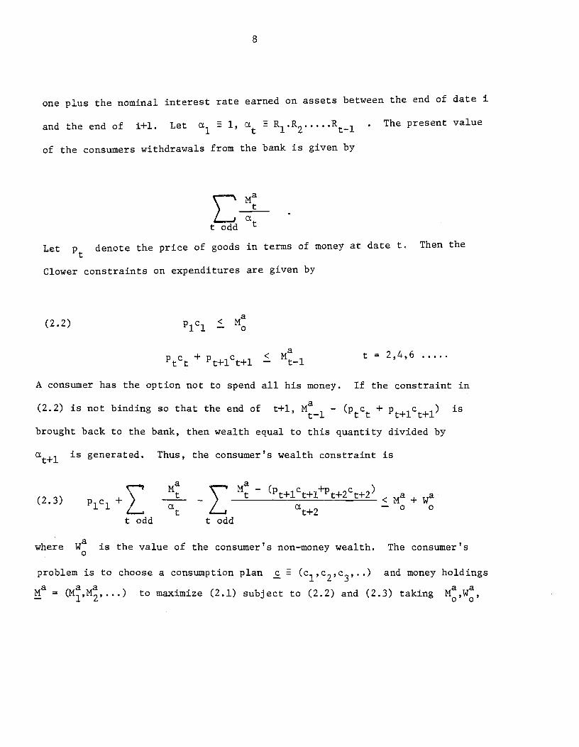
8

one plus the nominal interest rate earned on assets between the end of date i

and the end of 1+1. Let R1.R2. The present value

of the consumers withdrawals from the bank is given by

c' Mat

L_jc.todd

Let Pt denote the price of goods in terms of money at date t. Then the

dower constraints on expenditures are given by

(2.2) plc1< Ma— 0

+ pic1 < M t = 2,4,6

A consumer has the option not to spend all his money. If the constraint in

(2.2) is not binding so that the end of t+1, Ma (p c + p+ic+1) ist—l tt

brought back to the bank, then wealth equal to this quantity divided by

is generated. Thus, the consumer's wealth constraint is

Ma Ma — (pt+1ct÷i+p÷2c÷2) < Ma +(2.3) p1c1+ t t

at+2— 0 0

todd todd

where a is the value of the consumer's non—money wealth. The consumer's0

problem is to choose a consumption plan c (c1,c2,c3,..) and money holdings

Ma = (Ma Ma) to maximize (2.1) subject to (2.2) and (2.3) taking Ma,Wa,

9

prices and interest rates as given.

Note that we have not modelled the c-onsumer's decision about when to

go to the bank. He is being sent to the bank every other period. We could

add the decision about when to go to the bank by reducing the consumer's

wealth by some discounted transaction cost every time he decides to go to

the bank. In a steady state (i.e. where prices and interest rates are

constant) the consumer would then pick some fixed interval of time between

trips to the bank. We simply define the length of our period to be half

of that length of time. Unfortunately, it is probably true that, out of

the steady state, the consumer will not find it optimal to have a fixed

interval of time between trips to the bank. (However if the consumer faces

discrete choices of periods between trips to the bank, then there will be

an interval of price and interest rate paths "near" the steady state where

the consumer will not change his frequency of trips to the bank as the

economy moves away from the steady state due to say a "small" open market

operation.) Since we are taking the time between trips to the bank as exogenous

there is no point in keeping track of the transaction cost of going to the

bank. Thus it does not appear explicitly in (2.1) or (2.3).

Returning to the consumer's optimization problem, we assume that

u'(O) , u'(c) > 0, u''(c) < 0 and derive necessary and sufficient

conditions for a maximum. Note that for both the type a and type b

consumers' problems to have a solution, it is necessary that the price of a

bond which pays $1 forever to be finite, i.e.

(2.4)tl at

Note that > 1 since negative nominal interest rates make no sense.

10

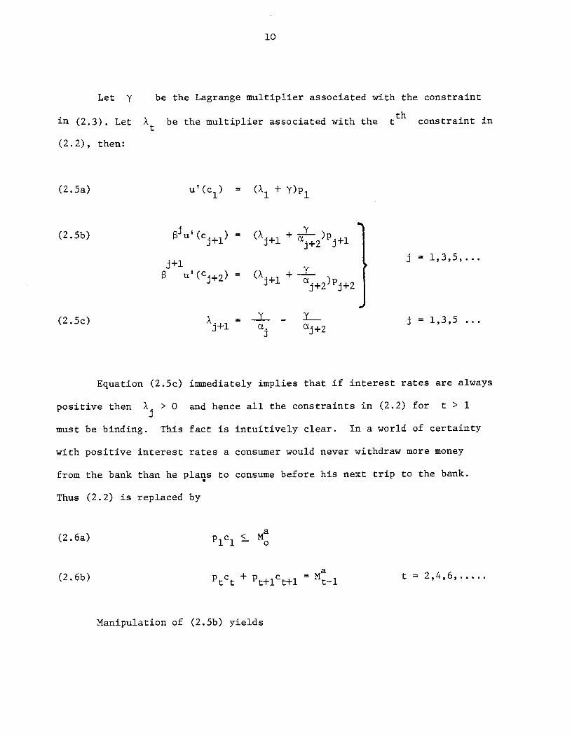
Let y be the Lagrange multiplier associated with the constraint

in (2.3). Let be the multiplier associated with the th constraint In

(2.2), then:

(2.5a) u'(c1) = (X1 + y)p1

(2.5b) &u'(c. ) = (X. +— )p•J+l Jl j+2 .3+1

j+l= 1,3,5,...

u' (c+) = (X1 +

(2.5c) = - j = 1,3,53+1 j+2

Equation (2.5c) inunediately implies that if interest rates are always

positive then X. > 0 and hence all the constraints in (2.2) for t > 1

must be binding. This fact is intuitively clear. In a world of certainty

with positive interest rates a consumer would never withdraw more money

from the bank than he plans to consume before his next trip to the bank.

Thus (2.2) is replaced by

(2.6a) p1c .. Ma

(2.6b) pc + p1c1 = M1 t = 2,4,6

Manipulation of (2.5b) yields

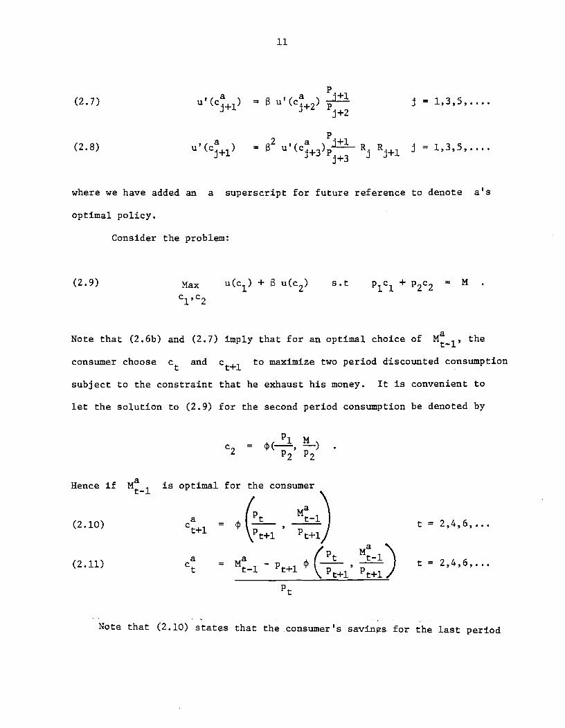
a , a j+lu (c+i) = j+2 P2

(2.8)

Max u(c1) + u(c2)

cl,c2St + p2c2 = N

Note that (2.6b) and (2.7) imply that for an optimal choice of N1, the

consumer choose c and c+i to maximize two period discounted consumption

subject to the constraint that he exhaust his money. It is convenient to

let the solution to (2.9) for the second period consumption be denoted by

lMc2 —__, —)

p2 p2

a a (P M1'\c = Mt_i— t+l

!÷i_______

Pt

Note that (2.10) states that the consumer's savings. for the last period

11

(2.7) j = 1,3,5

a 2 , a j+l R R j = 1,3,5u (c1 = u (c3) j+lj+3

where we have added an a superscript for future reference to denote a's

optimal policy.

Consider the problem:

(2.9)

Hence if M1 is optimal for the consumer

(2.10)

(2.11)

c+1 = t = 2,4,6,...

t = 2,4,6,...

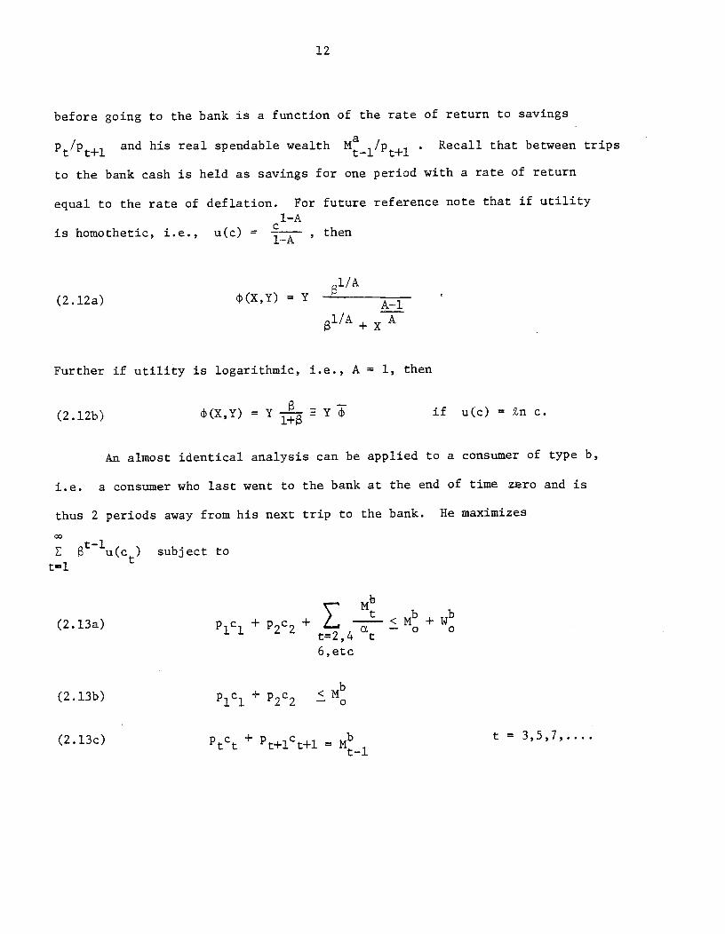
12

before going to the bank is a function of the rate of return to savings

and his real spendable wealth Mi/pt+i . Recall that between trips

to the bank cash is held as savings for one period with a rate of return

equal to the rate of deflation. For future reference note that if utility1-A

is homothetic, i.e., u(c) , then

IA

(2.l2a) (X,Y) = YA—i

el/A + A

Further if utility is logarithmic, i.e., A = 1, then

(2.12b) (X,Y) = Y E Y if u(c) = Zn c.

An almost identical analysis can be applied to a consumer of type b,

i.e. a consumer who last went to the bank at the end of time zero and is

thus 2 periods away from his next trip to the bank. He maximizes

t1t_lu(c) subject to

(2.13a) p1c1 + p2c2 + +

6,etc

(2,13b) p1c1 + p2c2< Nb

(2.13c) + +1+i = t = 3,5,7

13

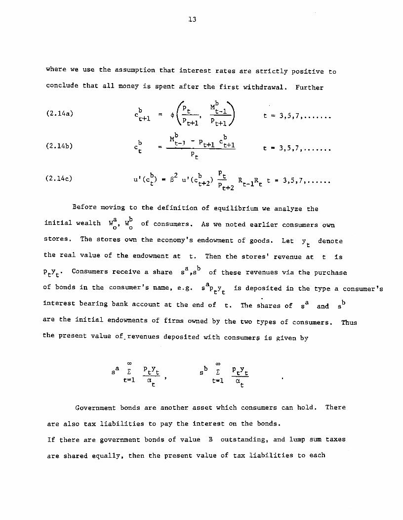
where we use the assumption that interest rates are strictly positive to

conclude that all money is spent after the first withdrawal. Further

bN(2.14a) cb+i =

t t1 t = 3,5,7t \t+l t+l

Nb —(2.14b) b t+1 t+1 = 3,5,7t pt

(2.l4c) u'(c) 2 u'(c+2) +2 RiR t = 3,5,7

Before moving to the definition of equilibrium we analyze the

initial wealth w, Wb of consumers. As we noted earlier consumers own

stores. The stores own the economy's endowment of goods. Let denote

the real value of the endowment at t. Then the stores' revenue at t is

Consumers receive a share 5a,8b of these revenues via the purchase

of bonds in the consumer's name, e.g. sapy is deposited in the type a consumer's

interest bearing bank account at the end of t. The shares of 8a and

are the initial endowments of firms owned by the two types of consumers. Thus

the present value of revenues deposited with consumerg is given by

b pyt=l ct

' t=l ct t

Government bonds are another asset which consumers can hold. There

are also tax liabilities to pay the interest on the bonds.

If there are goverument bonds of value B outstanding, and lump sum taxes

are shared equally, then the present value of tax liabilities to each

14

consumer is . Let Ba, Bb be the initial endowment of government bonds

held by a and b respectively. Hence the initial wealth of consumers net

of tax liabilities is given by

(2.15a) a = a____ + Ba B

o 2t=1 c

(2,15b) = bE + Bb 3

t=i 2

Note that in the statement of the consumer's optimization problem we

did not give consumers a demand for bonds. This is because in a world of

perfect certainty where consumers live forever, their lifetime consumption

opportunities are exactly described by present value formulae. A consumer

is indifferent as to how many bonds he purchases. The purchase of a

government bond by a consumer can be exactly offset by private borrowing.

That is, ac-consumer can keep his money—consumption plans constant and borrow

a dollar to buy a dollars worth of government bonds. The interest on the

government bond is used to pay the private loan, and nothing real has

changed. We have introduced government bonds into the model to facilitate

the analysis of open market operations.

15

2C. The Definition of Eqxi1ibrium

For expositional convenience we will be concerned with equilibria

where interest rates after date 1 are strictly positive, and where a

perpetuity has a finite price i.e., (2.4) holds. This allows us to use

the fact that all money withdrawn from the bank will be spent before a return

to the bank. An equilibrium is a price sequence2. (p1,p2,p3,..) and

an interest rate sequence R = (R1,R2,...) such that when all consumers

choose their consumption and money holdings optimally, all markets clear

(for all time).

Let C(2RMaWa) Ma(RMaWa) denote the optimal

consumption and money holding sequence for a consumer of type a, i.e. the

maximizer of (2.1) subject to (2.3),(2.6) and (2.15a). Similarly let

cb(RMbwb) and Mb(,R,Mb,wb) be optimal for the type b consumer.

ababNote that =(y1,y2,...), s ,s ,B ,B are exogenous.

Let be the total money supply at the end of period t. An

equilibrium price and interest rate sequence ,R, from the given initial

distribution of wealth and money is a solution to:

(2.16) C(,R,Ma,Wa) + c(,R,Mb,Wb) ytt 1,2,3

(2.17) M(,R,Ma,wa) + Mb(.,R,Mb,wb) = . = 1,2,3

A considerable simplification of these conditions is possible. In

particular we proceed to eliminate the interest rates and derive an equation

which relates the price path to that of output and the money supply.

Note that for t = 2, 4, 6,... M = — pc since the money

16

holdings of type a. at the end of t is composed of the withdrawal from the

bank at the end of t—l minus spending during period t. Hence (2.17)

implies that

(2.18a) M pc + M = M t = 4,6,8,..

If t = 4,6,8,,.., then M3 = — P—i—i = Hence (2.17) implies

that

(2,18b) M1 + pc = M1 t = 4,6,8,.,

Subtract (2.l8b) from (2.18a) and use (2.16) to derive

(2.19a) M = + M M1 t = 4,6,8,...

A similar argument shows that

(2.19b) Ma = p y + M5 — H5t t t t t—1 t = 3,5,7,...

Equations (2.19a) and (2.19b) give the flow equilibrium in the money

market. The left hand side of each equation is the money withdrawn from the

bank at the end of period t. The right hand side gives the money flowing

into the bank at time t. Inf lows are composed of the value of expenditures

plus the value of monetary injections M - M_1. The monetary

injections are used to buy bonds at the ttbank!t (i.e., the asset market). An

open market operation increases the money flowing into the bank and this

17

necessitates an increase in withdrawals to maintain money market equilibrium.

Substitution of (2.l9b) into (2.17), and using the fact that for t = 3,5,7,..b b

Mt = (2.14) and (2.19a) yields

_____ 1 t—l t—(2.20) + M—M1 + tlt + MS —N5

2 =t+1

The above substitution makes (2.20) correct for t = 3,5,7. A similar

substitution of (2.19a), etc. into (2.17) shows that (2.20) is true for

t = 4,6,8,... as well. Equation (2.20) is another statement of the stock

equilibrium for money in (2.17). The term py + MS — N5 is the moneyt t t—1

held at the end of t by those who go to the bank at the end of t. The

next term is the money holdings of those who go to the bank at the end of

t+1. Their money holdings are exactly enough to finance their consumption during

period t+l, namely

Equation (2.20) is a second order difference equation in Pt. To

get some initial conditions we consider (2.16) and (2.17) for t = 1 and

t = 2. We have not shown that with interest rates positive, consumers will

exhaust their initial money holdings before arriving at the bank for the

first time. Whether this is optimal or not depends on the benefit of savings

in the form of money from date 1 to date 2 p1/p2 for the type a consumer,

p1and — for the type b consumer. If rates of return are high enough relativep3

to their rate of time preference then they may not spend all their money until

after their first trip to the bank. Some simplification is achieved if we

restrict ourselves to equilibria where it is optimal for them to exhaust.

In this case

18

(2 21)a

Ma + b — Mbplc1 = o

Using an argument similar to that given in the derivation of (2.20) we

conclude that

(2.22a) p1y1 + M — MS + p Mb2çP2'P2)

= M

(2,22b) p2y2 + M M + (p2 p1y1 + M = MP3

Nominal interest rates can be derived as a function of the price path

as follows. Use (2.14c), the fact that c = y — c, (2.10), and (2.19b) to

derive

at R R t = 3,5,7,...(2.23a) u'(yt c) = 2u'(y+2 -c+2) t+2 t

nt-i -2'+ MS - MS

(2.23b) c =Pt' Pt

t = 3,5,7,....._____ t—2 t—2 t

Similarly use (2.8), c = y — c, (2.14a) and (2.19a) to derive

b Ptb — R R t = 2,4,6,8,...(2.23c) u'(y — c) = 2u'(y+2 —ct+2) t+2 t—l

+MS M5— t = 4,6,8,...b

(Ptit—2t—2 t-—2 t

(2.23d) c =

t Pt

In (2.23b) and (2.23d) we assume that (2.21) holds, otherwise t must start

two periods later. Under (2.21) the initial values of c and c are given

by

19

(2.24) c = cP

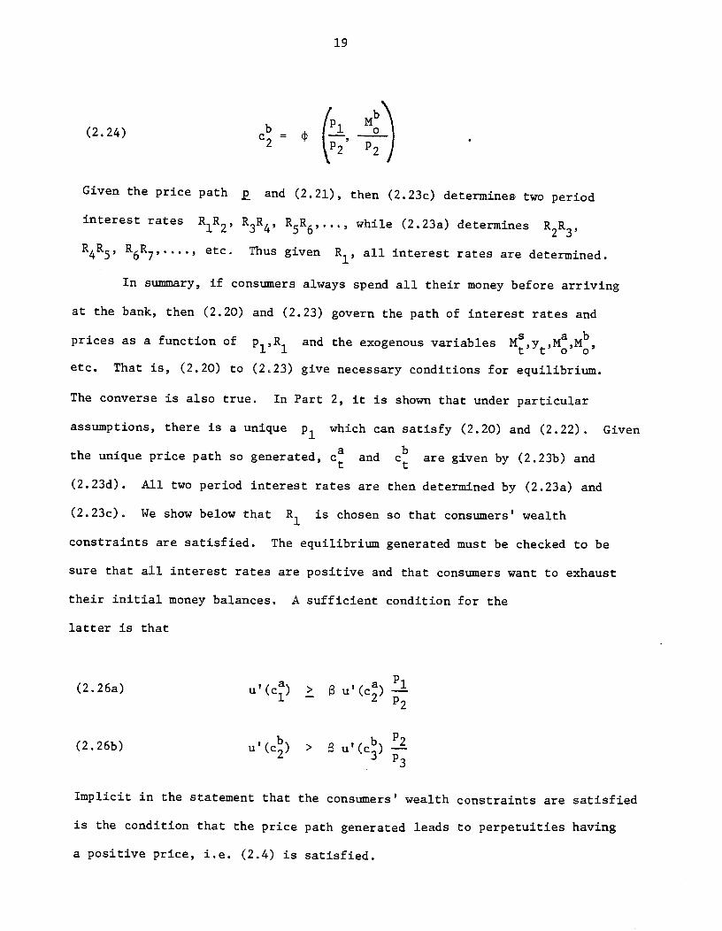
(, P')Given the price path and (2.21), then (2.23c) determines two period

interest rates R1R2, R3R4, R5R6,...,, while (2.23a) determines

R4R5, R6R7 , etc. Thus given R1, all interest rates are determined.

In si.umiary, if consumers always spend all their money before arriving

at the bank, then (2.20) and (2.23) govern the path of interest rates and

prices as a function of p1,R1 and the exogenous variables

etc. That is, (2,20) to (2,23) give necessary conditions for equilibrium.

The converse is also true. In Part 2, it is shown that under particular

assumptions, there is a unique p1 which can satisfy (2.20) and (2.22). Given

the unique price path so generated, c and c are given by (2.23b) and

(2.23d). All two period interest rates are then determined by (2.23a) and

(2.23c). We show below that is chosen so that consumers' wealth

constraints are satisfied. The equilibrium generated must be checked to be

sure that all interest rates are positive and that consumers want to exhaust

their initial money balances. A sufficient condition for the

latter is that

(2.26a) u'(c) > u'(c) —ip2

b b(2.26b) u'(c2) > u'(c3)

—p3

Implicit in the statement that the consumers' wealth constraints are satisfied

is the condition that the price path generated leads to perpetuities having

a positive price, i.e. (2.4) is satisfied.

20

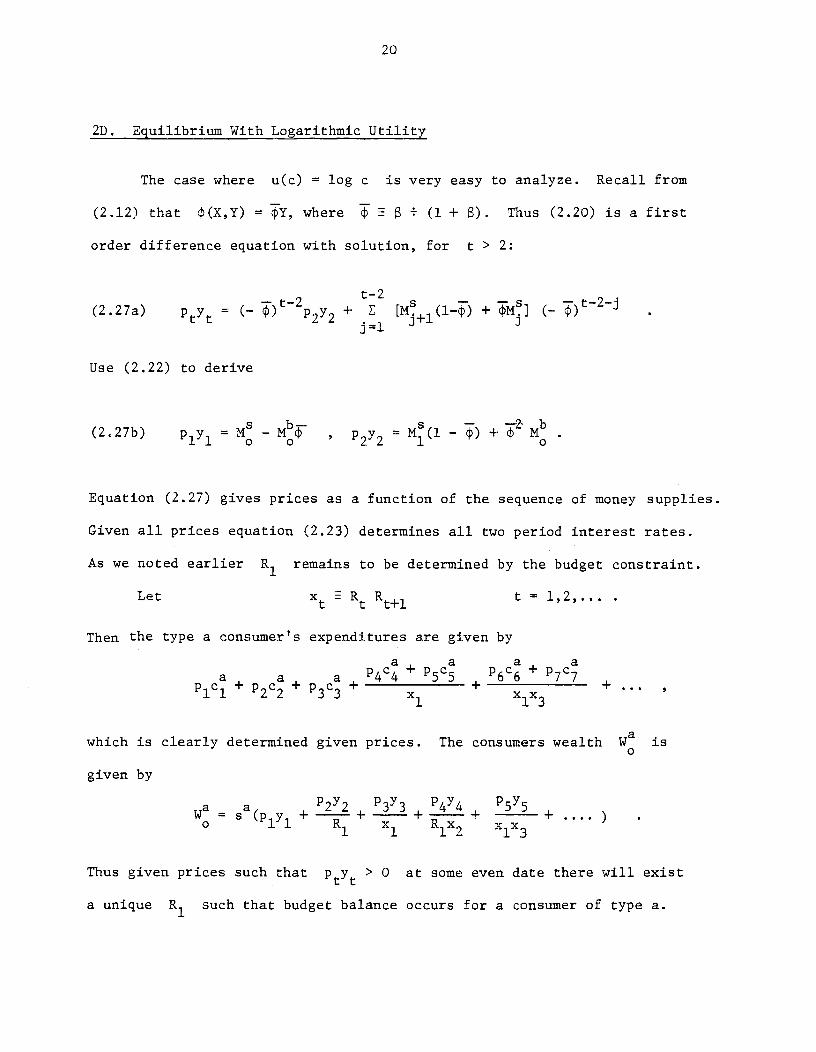
2D. Equilibrium With Logarithmic Uti1Z

The case where u(c) = log c is very easy to analyze. Recall from

(2.12) that (X,Y) = cY, where E (1 + ). Thus (2.20) is a first

order difference equation with solution, for t > 2:

(2.27a) py ( )t2 + {M1(l) + M] (

Use (2.22) to derive

(2.27b) p1y1 = — , p2y2= M(l — + -2 Mb

Equation (2.27) gives prices as a function of the sequence of money supplies.

Given all prices equation (2.23) determines all two period interest rates.

As we noted earlier R1 remains to be determined by the budget constraint.

Let x Rt Rt÷1 t = 1,2

Then the type a consumer's expenditures are given by

a a a aa a a p4c4 + p5c5 p6c6 + p7c7

PI_ci + + p3c3 +x1

+x1x3

+

which is clearly determined given prices. The consumers wealth is

given by

a a 22 33 p4y4 p5y5W=s(py+ + + + +....)o 1 1R1 x1 R1x2 x1x3

Thus given prices such that py > 0 at some even date there will exist

a unique R1 such that budget balance occurs for a consumer of type a.

21

This R1 along with the prices generated by (2.27) and x generated by

(2.2,3) form an equilibrium. It will be clear from our later discussion

that (2.26) is satisfied for a range of values of Ma and Mb near the

steady state which is to be defined below. Thus since (2.27) gives a

unique price sequence after date 2, we have found a unique equilbrium price

and interest rate path for all dates assuming that initial money balances

are exhausted before the first arrival at the bank.

22

3. The Steady State Distribution of Cash Balances

As is clear from the last Section the model finds a price path from

the initial distribution of money and the path of monetary injections. It

is worthwhile to consider the initial distribution of cash balances, which

when there are no new monetary injections, maintains itself over time. If

M H, eq. (2.19) implies that the distribution of cash will be constant if

and only if spending py is constant. If y is not constant then the

real interest rate will not in general be constant so we will be unable to

maintain spending constant. Hence we assume that y is constant, i.e.,

yt =

We can use (2.20) to get an equation of the relationship between

prices, money and output when all three are constant:

(3.1) y + (l,y) =

Thus in the steady state money is neutral in the sense that a proportional

increase in total money raises prices by the same proportion (recall that

output y, is exogenous). From (2.19) the money holdings of someone who

makes a withdrawal at the end of t is given by M for t odd, for

t even:

a b _____(3.2) M1=M=py y+(l,y) H

The money holdings at the end of t of someone who goes to the bank

at the end of t+l, must satisfy + = N. Hence we have

23

(3 2b) Mb = Ma (1,y) M1 o y+(l,y)

Note that Ma Mb = Ma = Mb = Ma etc. and Mb = Ma M' = Ma etc. ino 1 2 3 4 o 1 2 3

the steady state.

It is important to note that in the steady state Ma < Mi'. That is,

someone who has two periods to go before his trip to the bank has more money

than someone who has only one period to go. To see this note that l,y)

is the consumption of someone is in the last period before his trip from

the bank, and y — 1,y) is the consumption of someone who is in the

first period after his trip to the bank. The assumption that u'(O) =

implies that y — (l,y) > 0. Hence

(3.3) M < M, Ma < Mb, etc.

Equation (3.3) will be a key ingredient in showing that if the

economy begins in a steady state, then an open market operation is not

neutral (even with homothetic preferences).

Note that consumption is the same for each individual in every other

period. Thus from (2.23) the two period interest factor is

—2(3.4) R1R2 — R2R3

— ... —

This determines all interest factors as a function of the initial factor

R1. If the economy begins with the steady state distribution of money

(Ma,Mb) as in (3.2), then consumers of type b begin with more money. Hence

if they get the same share of output (i.e. 5a = Sb) and have the same

amount of government debt (Ba = Bb), they will have different total wealths.

24

But, for the distribution of cash balances to maintain itself over time

the consumers must have the same spending pattern. This is achieved via

the nominal rate in the first period taking on a value which permits the

financing of steady state expenditures. Thus, the present value of a type

a consumer's expenditure is given by

p.c.+p.+ic.+i Pp1c1 + E

1 1 1 1 = P((l,y) + y +RR +R R R R+ = P l,y) +

2ieven i—i 12 1234 /

Th total wealth of the consumer is, from (2.15) and (3.2)

Ma + 5a + - = Ma + Ba -! + 5ap (1 + __ + + i +i=l 1 1 12 12R3

= P(1,y) ÷Ba_ + 5a (l+++...) + ____(l÷2+..)2 R

1

(3.5) Ma + = P(1,y) + Ba - +

Thus equilibrium requires that

__(3.6) 2

i_2R)

i_2a a

a B s — SFor exanmie if B = —, then R = — z —

2 1 a b1—s s

Thus if the two types of traders have the same net government debt and the

same share of the firms, the initial nominal interest rate is zero!! This

peculiarity arises out of the fact that a steady state requires that the

two types be in a symmetric position. However, if we start the system at a

25

steady state distribution of money we automatically put the type a consumer

in a worse position whenb

and 3a = Bb. There are three sorts of

differences among the two type when Ba Bb and a 5b i.e. when

wb. First, the type b consumer will have a higher present value of

consumption. This is because

(3.7) y - (l,y) > (l,y)

which can be seen from (2.7), (since prices are constant, marginal utility

of consumption declines at the rate of time preference from the time of

arrival at the bank until the next return), Thus, consumption alternates

between the two types with type b getting the high consumption first. A

second important difference between them is that when = Wb, the type b

consumer begins with a higher wealth since Mb > Ma by (3.3). The third

and most important difference is that a type b trader will earn one periodTs

interest on his wealth before returning to the bank. This last effect is

related to the other two. This can be summarized by looking at the difference

between wealth and the present value of expenditures in equilibrium for the

two types:

- (p12) + - +RRR3

+R1R2R3R4R5

all the two period interest factors R.R. = —2 ThereforeJ J+1

value of expenditures not financed by initial cash balances for

a a +a_p(+ + +Mo p1c1 o

R1R2 R1R2R3R4

Recall that

the present

26

a is times the corresponding quantity for b. Thus the extra amount of

money which b holds has the effect of allowing him an extra period of interest

before he must withdraw money from the bank to finance his future consumption.

Clearly the above two quantities can equal zero only if R = 1, which destroys

b's advantage.

We are trying to model a timeless steady state. We don't have some

particular initial date in mind for starting the economy. Thus there is no

particular date at which the interest rate is 0. The only interest rate

which will maintain itself for all time including the initial date satisfies

R 1From (3.6) this will be the case when

(3.8) Ba = Bb if S(l + ) = 1,

which implies 5a > .5, since < 1. Alternatively a = b = .5 then

2L.. . > 02

In suniary the steady state will involve type b holding more initial money

but less of the initial share of other nominal assets than the type a consumer.

It is essential to note for what follows that the steady state involves type a

holding more interest earning assets than type b. Thus, when we analyze an open

market operation which increases the price level in an unanticipated way at date 1,

wealth will be redistributed from b to a. That can be looked at from two points

of view. First, since b holds more money, inflation yields him a real wealth loss.

Second this wealth loss is transferred to the type a consumer via a lower nominal

interest rate to finance his withdrawals of money at date 1. That is, it is

helpful to think of b as lending the wealth to use from the end of date 1 to the

end of date 2 to finance part of a's withdrawal from the bank at the end of 1.

27

These points will be reviewed after analyzing the effect of an open market

operation.

Before proceeding to open market operations, we note that in the steady

state all consumers find their initial cash in advance constraint strictly

binding. That is, the inequalities in (2.26) will be strictly binding when

< 1. This means that we can consider small perturbations about the steady

state which maintain strict inequality in (2.26). Thus, in what follows we

will implicitly be restricting ourselves to small enough perturbations that

the initial cash in advance constraint is binding.

28

4A. The Neutrality of Helicopter Monety Injections

It is of some expository value to consider the effect of a monetary

injection which creates a proportional increase in everyone's money holdings.

Since some consumers are not at the bank, the government must literally

deliver cash to them. (In a continuous time model only a small

fraction dt of consumers will exhaust their money holdings between t and

t+dt. Thus, the government will have to deliver cash to almost everyone in

the economy.) Formally this involves considering what new equilibrium will

correspond to initial money endowments (l+k)Ma, (l+k)Mb. That is, the

government increases everyone's cash balances by k percent at time zero

and from then on there are no monetary injections.

We will show that it is an equilibrium for all prices Pt to be k

percent higher than they would have been had there been no monetary injection,

and that all interest rates and consumptions are unchanged. In the case where

Ba B12 it is important to clarify our assumption about taxes. We assume

that real taxes are kept constant, and the real value of government debt is

held constant. It is convenient to assume that the real value of debt is

held constant by a proportional increase in Ba and Bb. Under these

assumptions a k% increase in prices with constant interest rates will

raise Ba_B,2 by k percent. If we do not keep the real net debt constant

for each individual then the open market operation will redistribute wealth

due to a change in the tax burden relative to the value of endowed

goverment debt. In this case the analysis given below will require a slight

modification, as indicated after the proof of the simple case.

To see that helicopter injections are neutral note from (2.7) and

29

(2.8) that the consumers irt ordei condItion for bDtimal consumptidii

will still be satisfied at the old consumption levels when prices are

multiplied by (l+k), and interest rates are unchanged. Note that the

initial cash in advance constraints (2.2) and (2.13b) will be satisfied

at the old consumption levels when Ma,Mb,P1 and p2 are multiplied by

l+k. Thus, the only thing left which must be verified is that consumers

can afford their old allocation at the new prices. As can be seen from

(2.15) nominal wealth rises by k percent. Hence at the old consumption

levels the present value of nominal spending is unchanged. Thus if the old

allocations formed an equilibrium, then they will still be an equilibrium

with Pt multiplied by l+k, and interest rates unchanged.

Now consider the case where a wealth redistribution occurs due to

the real tax burden changing for individuals. Again multiply all prices

by l+k and keep all 2—period interest rates constant. (i.e., keep

R1R2,R2R3,... all constant). If all consumptions are held constant, then

all first order conditions in (2.7),(2.8) are satisfied. There is one problem

with maintaining this as an equilibrium, namely if is unchanged then

either type a or type b consumers will be violating their wealth constraint,

since the value of total wealth does not increase by k% for each consumer.

As we noted earlier the first order conditions involve only two period

interest rates. All interest rates are determined once R1 is chosen. We

noted that R1 is chosen so that consumers can afford the consumption path

assigned to them by the first order conditions. Thus we can choose a new

R1 so that the old level of consumption is affordable by say type a. (Note

that if markets clear and an allocation is affordable by type a then it is

30

affordable by type b). Hence an open market operation which redistributes

wealth between type a and type b consumer will be neutral except that the

one period interest rate changes——all two period rates will be unchanged.

This effect is not likely to be of great importance. It is difficult to

see why there would be significantly different real tax burdens associated

with differences in the day individuals go to the bank

Note that the above neutrality results hold independent of whether

the economy begins at the steady state cross sectional distribution of

cash balances.

4.B. The Non—Neutrality of Open Market Operations

We consider the effect of an open market operation given that the

economy is in a steady state before the operation. Further, the operation

is a once and for all unanticipated event. An open market operation involves

the purchase or sale of government bonds for money. In a purchase of bonds

the government buys bonds on the asset market (i.e. at the "bank"). The

sellers of the bonds will have more money. Consumers who are at the bank

or who are not at the bank are assumed to be able to sell bonds costlessly

to the government. (Recall the term "a consumer not at the bank at time

means a consumer who has not yet depleted his cash balances.) When a

consumer who is not at the bank sells the bond for cash, it is optimal for

him to immediately convert the cash back to bonds. Thus equilibrium will

involve only those people who are at the bank at time t holding the cash.

That is, we assume that the major transaction cost involves transportation

to the bank to increment cash balances. Thus a small open market operation

will not make it optimal for a consumer who has not yet exhausted his cash

31

balances to go to the bank and increment them.

If there is a transaction cost of converting bonds into money, as

well as a cost of transportation to the asset market, then those consumers

who have not yet exhausted their cash balances will not find it optimal to

sell bonds to the government. For if they did so they would have to sell

bonds for cash which would have to be converted back into bonds and then

converted back again into cash when they exhaust their money balances

Thus, in this case also, it is an equilibrium for only those consumers at the

bank to increase their money holding in response to the open market operation.

Note that we assume that the open market operation is sufficiently small so

that it is still optimal for consumers to wait two periods before returning

to the bank after their last withdrawal.

Similar remarks apply to an open market sale of bonds by the

government. Here it is important to note that cash flows into the bank from

the stores that sell goods (i.e., firms are purchasing bonds for the consumers

that own the firms on the asset market). The open market operation is

sufficiently small to keep consumers who have not yet exhausted their cash

balances from going to the bank. Thus in equilibrium the consumers who have just

exhausted their cash balances will find it optimal to withdraw less money when

the government sells bonds.

We begin with a formal proof that an open market operation is not

neutral and then proceed to analyze dynamic effects associated with an

open market operation, First it is important to do some accounting.

Recall that Ba and Bb represent the nominal value of the government debt

32

that a and b are endowed with. Before the open market operation

Ba + Bb = B where B is the total present value of the tax liabilities

associated with the open market operation, which equals the total stock of

government bonds. If an open market operation occurs at the end of period

1, which is announced at the beginning of period 1, there is no automatic

increase in individuals' endoinents of government bonds or money. Prices

and interest rates adjust so that individuals find it optimal to hold the

new money and bonds. However, there is an automatic change in individuals'

tax liabilities just after the announcement. If the increase in the stock

of bonds is LB, then the total present value of tax liabilities rises by

AB. Again it is convenient to assume that the distribution of the tax burden

does not change so that each individual's tax liability goes up by . We

also assume that Ba = Bb for convenience. Note that an open market operation

means that

(4.1) AB + MS — M5 = 0,1 0

where M5M+Ml)

From period 1 on, the total money supply will be constant, M = M, t > 1.

As in Section 4.a consider a k percent increase in the money supply,

i.e. M = (l+k)M5. We first show that if is the equilibrium

corresponding to k = 0, with the initial cash in advance constraints strictly

binding, then it cannot be an equilibrium for all prices to rise by k

percent, and for all two period interest rates and consumption to be unchanged.

This is an immediate consequence of the cash in advance constraint for consumers

— a a — b — b b ,, ,,of type a and b: p1c1 = M, p1c1 + p2c2 = M, where the bars above

33

prices indicate post—announcement prices. Since cash on hand is unchanged, if

prices increase by k percent, (i.e. =(l+k)p1 after the announcement)

then it is not feasible for c to be unchanged. It might be thought

that this is some initial period effect which disappears, but that is quite

wrong. If prices rise by k% above what they would have been with k = 0, then

c must be lower than it would have been and c must be higher, since

a b bc1 + C1 = y1. Thus c2 must be lower than it would have been. Further,

from equation (2.19b)

(4.2) =p1y1 + AN,

where we recall that (2.19b) holds for t = 1, when the cash in advance

constraint is binding. Equation (4.2) implies that when prices increase by

k percent the monetary withdrawal of the type a consumer increases by more

—b . bthan k/.. Recall also that c2 is lower than c2, hence a s consumption

c must rise to , and from (2.7) c must also rise. This is financed

by the ! being larger than (1+k)M when =(l+k)p1. It follows

that < c, and thus c > c because with =(l+k)p2 and

M2 = p2y2 by (2.19a), nominal spending p3c3 + p4c4 must rise by k/.. A

consequence of c rising is that c must fall. But using (2.8) the

fall in c and the rise in c must imply that the nominal interest factor

R1R2 falls. This not only shows that it is not an equilibrium for all prices

to increase by k% keeping interest rates and consumption constant, but

illustrates how monetary shocks can persist. Of course, it need not be

an equilibrium for = (l+k)p, but the fall in the interest rate R1R2 to

34

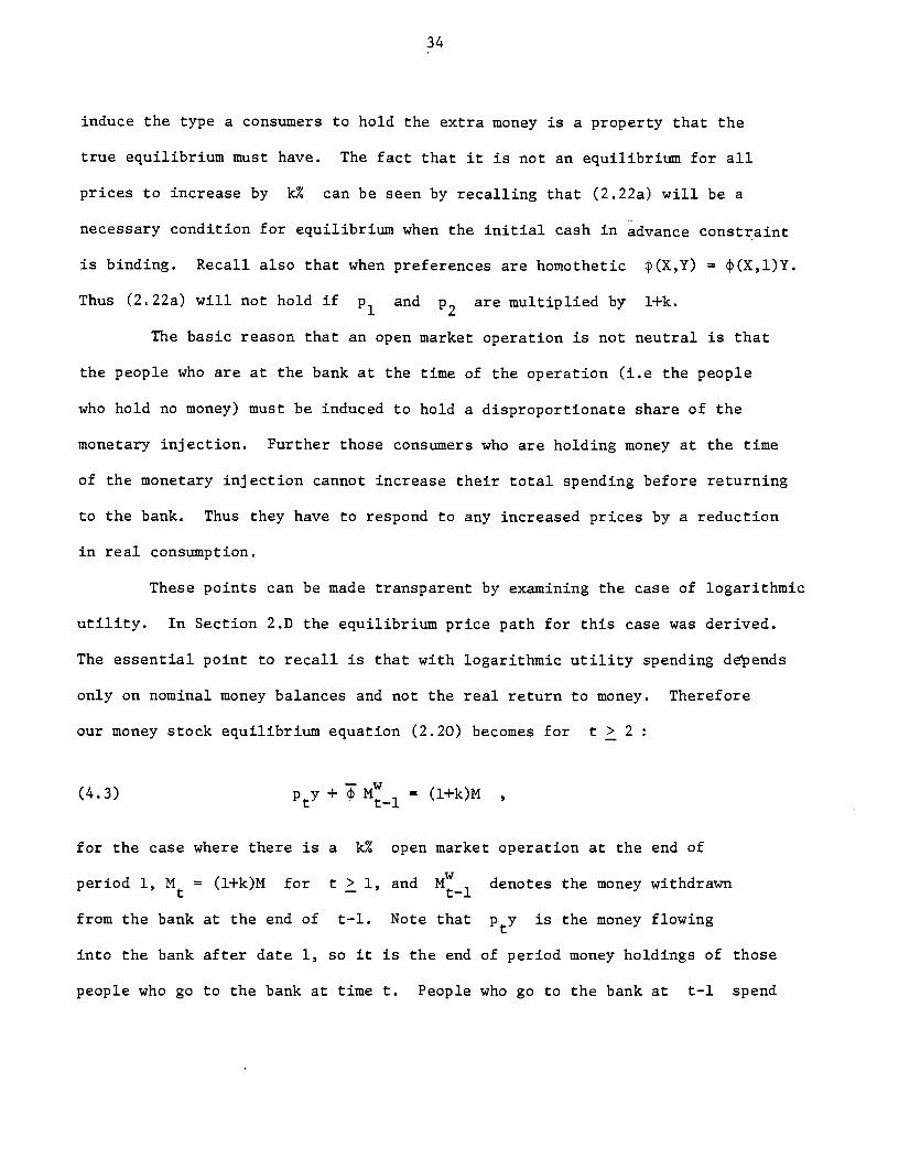
induce the type a consumers to hold the extra money is a property that the

true equilibrium must have. The fact that it is not an equilibrium for all

prices to increase by k.% can be seen by recalling that (2.22a) will be a

necessary condition for equilibrium when the initial cash in advance constraint

is binding. Recall also that when preferences are homothetic 4(X,Y) = (X,l)Y.Thus (2.22a) will not hold if p1 and p2 are multiplied by l+k.

The basic reason that an open market operation is not neutral is that

the people who are at the bank at the time of the operation (i.e the people

who hold no money) must be induced to hold a disproportionate share of the

monetary injection. Further those consumers who are holding money at the time

of the monetary injection cannot increase their total spending before returning

to the bank. Thus they have to respond to any increased prices by a reduction

in real consumption.

These points can be made transparent by examining the case of logarithmic

utility. En Section 2.D the equilibrium price path for this case was derived.

The essential point to recall is that with logarithmic utility spending de'pends

only on nominal money balances and not the real return to money. Therefore

our money stock equilibrium equation (2.20) becomes for t > 2

(4.3) py + M1 = (l+k)M

for the case where there is a k% open market operation at the end of

period 1, M = (l+k)M for t > 1, and denotes the money withdrawn

from the bank at the end of t—l. Note that py is the money flowing

into the bank after date 1, so it is the end of period money holdings of those

people who go to the bank at time t. People who go to the bank at t-l spend

35

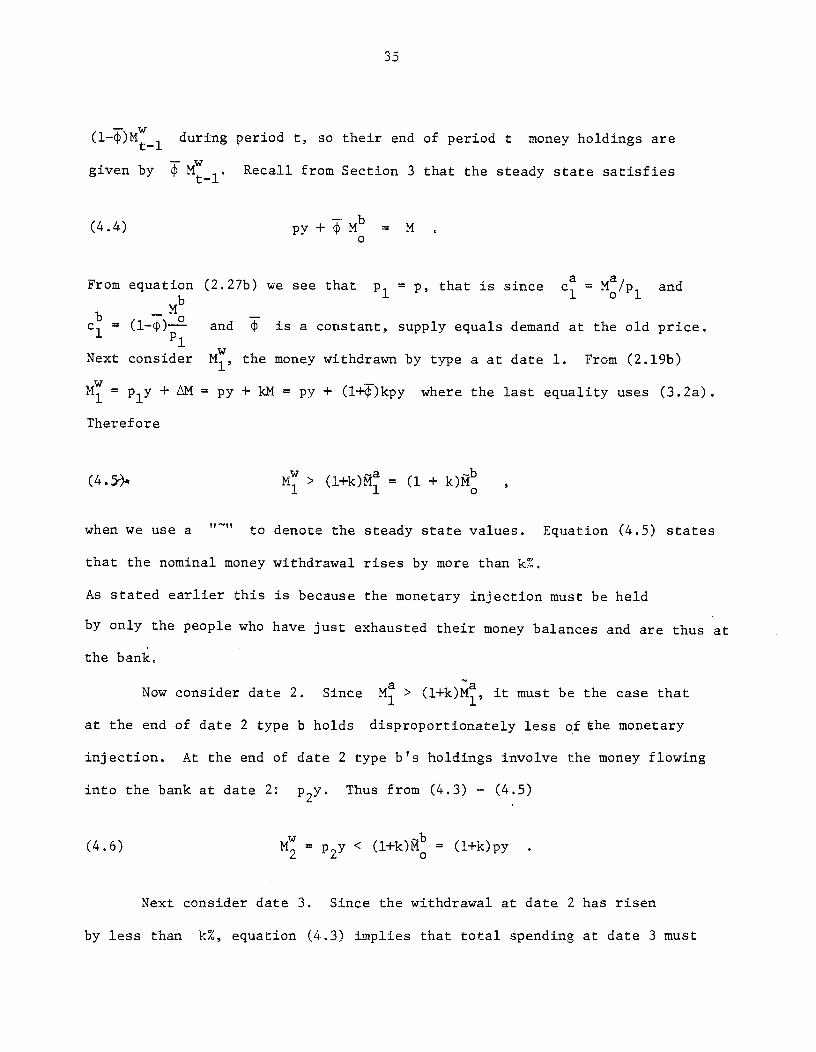
(1_q)M1 during period t, so their end of period t money holdings are

given by M1. Recall from Section 3 that the steady state satisfies

(4.4) py+Mb = M

From equation (2.27b) we see that p1 = p, that is since c =Ma/P1 and

bMb

c1 = (1—q)—2- and is a constant, supply equals demand at the old price.

Next consider M, the money withdrawn by type a at date 1. From (2.1gb)

=p1y + M = py + kM = py + (l+)kpy where the last equality uses (3.2a).

Therefore

(4.)m M > (I+k)! = (1 + k)

when we use a "" to denote the steady state values. Equation (4.5) states

that the nominal money withdrawal rises by more than k%.

As stated earlier this is because the monetary injection must be held

by only the people who have just exhausted their money balances and are thus at

the bank.

Now consider date 2 Since M > (1+k)M, it must be the case that

at the end of date 2 type b holds disproportionately less of the monetary

injection. At the end of date 2 type b's holdings involve the money flowing

into the bank at date 2: p2y. Thus from (4.3) (4.5)

(4.6) M p2y < (1+k)& = (l+k)py

Next consider date 3. Since the withdrawal at date 2 has risen

by less than k%, equation (4.3) implies that total spending at date 3 must

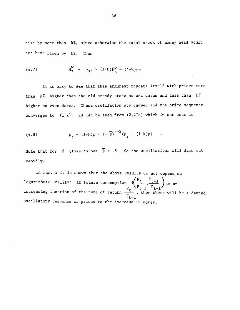
36

rise by more than k%, since otherwise the total stock of money held would

not have risen by k%. Thus

(4.7) p3y > (l+k)& = (l+k)py

It is easy to see that this argument repeats itself with prices more

than k% higher than the old steady state at odd dates and less than k%

higher on even dates. These oscillation are damped and the price sequence

converges to (l+k)p as can be seen from (2.27a) which in our case is

(4.8) Pt = (1+k)p + ( )t2( - (l+k)p)

Note that for close to one .5. So the oscillations will damp out

rapidly.

In Part 2 it is shown that the above results do not depend on

logarithmic utility: if future consumption M1)

is an

Pt Pt+lincreasing function of the rate of return , then there will be a damped

t+loscillatory response of prices to the increase in money.

37

4C. 'fhe Effect of anenMarket Operation on Interest Rates

As we showed below an open market operation must cause prices and

interest rates to move in such a way that consumers at the bank are

temporarily willing to hold more than their steady state share of money.

The cost of holding money as opposed to bonds to the consumer who is at the

bank is the two period nominal interest rate. The cost of holding (i.e.,

withdrawing) money to increase current consumption is related to the two

period real rate of interest. Thus we should expect that the two period

real and nominal rates to fall. Indeed for the logarithmic case this is

true, as we show next. This is extended to a more general case in Part 2.

Use (2.8) for the log case to derive

a — ap,c, (l—)M. p.,y

(4.9) RR = =.12 a —ap1y+LN

Use (2.19) and the definition of the steady state to derive

p3y = M5 -cM

= MS MS — (MS —

Thus

(4.10) 2R1R2 = M(l±k)(l—) + 2 = (l2) [1÷k] -2

The right hand side of (4.10) is a convex combination of 1 and a term less

than 1. Hence

< 1.

For t > 1

38

(4.11) 2RtRt+l =M2 = p2

t

Recall that from (4.8) Pt oscillates with declining magnitude of

oscillation. Therefore t+2't will fall below the steady state value of

2RR+i which is unity. Note that as Pt converges to (l+k)p, 2RtRt+i

converges to its old value of unity.

Finally, the initial interest rate R1—l must fall. As we noted

in Section 3 the initial interest rate is chosen so that the wealth constraint

holds. We choose the steady state with lump sum taxes to pay interest and

where (3.8) holds. Recall that in the steady state Nb > Ma and 9a >0 0

When prices rise the type b consumer takes a capital loss on his initial

money endowment. Recall that the type b consumer in effect lends money to

the type a consumer, since the type a goes to the bank and makes a withdrawal

at the end of date 1 while b waits until the end of date 2. The increase

in wealth to the type a consumer will appear as a drop in the interest rate

R1—l in his implicit cost of going to the bank one period earlier.

The above statements can be proved by direct calculation for the

case of logarithmic utility. To see this use (4.9) and (4.11) to obtain:

p +1 p1y+iN(4.12a) R = R t 3,5,7t

Pt1

t+l 1 _______(4.l2b) R = t = 2,4,6t

PtR1 p1y+iN

The present value of the expenditures of a type a consumer can be found

39

using (4.12), (2.6b), and (2.l9b) to satisfy:

Ma 2(4.13) p1c + =

p1c + + +2

t=24, .. t—1

Recalling that (3.8) holds in the steady state, Ba = Bb = B/2 ,that for an

open market operation + B 0, and that each person's new tax liability

becomes (B + B) '-i- 2, we can compute the wealth of the type a consumer:

(4.14) Ma + Ba — B+/B + a = Ma + + a +2t=1 t °

1 (l—)

2

+ (p1y+iM) 21—

Equate the present value of expenditure (4.13) to wealth in (4.14) and use

the facts that iN kM, (3.8), (3.1), (3.2), (1,y) E [+(l+)]yMa p1c, to derive

(4.15) R1 [1 +1±2]

÷ + k(l+2) (i+22) ]

WriteR1 + e, Note that

sign(e) = sin( l+2- + k(1+2)(1

sign(e) =

The assumption 0 < < 1 implies that sign(e) = — sign(k). Hence an

increase in the money supply causes the initial one period nominal rate to

fall below its steady state value of Since p2 > p1, the real rate

also falls.

40

5. Conclusion

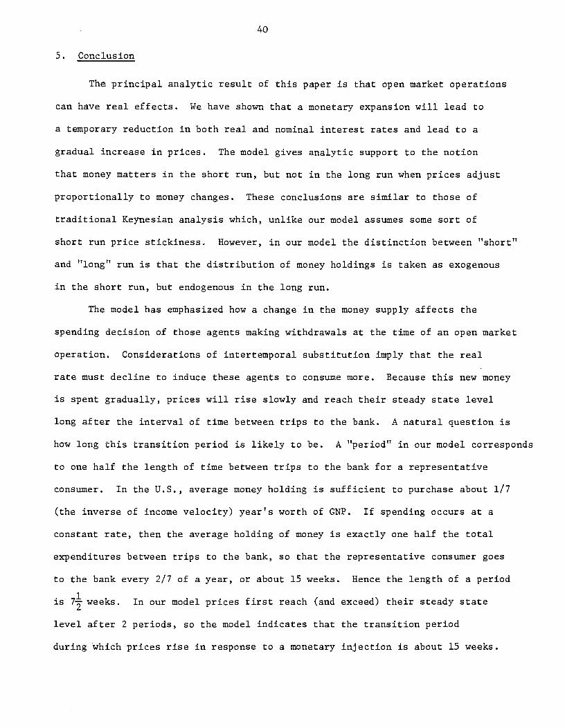
The principal analytic result of this paper is that open market operations

can have real effects. We have shown that a monetary expansion will lead to

a temporary reduction in both real and nominal interest rates and lead to a

gradual increase in prices. The model gives analytic support to the notion

that money matters in the short run, but not in the long run when prices adjust

proportionally to money changes. These conclusions are similar to those of

traditional Keynesian analysis which, unlike our model assumes some sort of

short run price stickiness. However, in our model the distinction between "short"

and "long" run is that the distribution of money holdings is taken as exogenous

in the short run, but endogenous in the long run.

The model has emphasized how a change in the money supply affects the

spending decision of those agents making withdrawals at the time of an open market

operation. Considerations of intertemporal substitution imply that the real

rate must decline to induce these agents to consume more. Because this new money

is spent gradually, prices will rise slowly and reach their steady state level

long after the interval of time between trips to the bank. A natural question is

how long this transition period is likely to be. A "period" in our model corresponds

to one half the length of time between trips to the bank for a representative

consumer. In the U.S., average money holding is sufficient to purchase about 1/7

(the inverse of income velocity) year's worth of GNP. If spending occurs at a

constant rate, then the average holding of money is exactly one half the total

expenditures between trips to the bank, so that the representative consumer goes

to the bank every 2/7 of a year, or about 15 weeks. Hence the length of a period

is weeks. In our model prices first reach (and exceed) their steady state

level after 2 periods, so the model indicates that the transition period

during which prices rise in response to a monetary injection is about 15 weeks.

41

This empirical issue is complicated by the fact that the monetary intermediation

channels in the actual economy are more intricate than those of our model. Our

estimate is likely to underestimate the duration of the transition period to

the extent that firms hold idle balances and do not instantly transmit their

proceeds to the bank. However, this estimate is too long if some consumers

receive cash payments directly, without having to make withdrawals.

There are other reasons to suspect that monetary inpulses will have a more

delayed response than suggested by the model. If the time between trips to the

bank were made endogenous, rather than the fixed interval assumed in the model,

then it could be imagined that the decline in nominal interest rates would induce

a longer time before the next return, as the cost of holding money goes down.

In this case the new money would be spent more gradually than the case presented

in this paper, and the price rise would be slower and longer. Similarly, the rate

of spending for the recipients of the new money would not have to rise as much;

the decline in real rates would be lower than the model's conclusion.

Some of the model's conclusions are very different from those of earlier

theories. The Clower cash in advance constraint makes current prices less sensitive

to anticipation of future money than suggested by the analysis of Sidrauski (1976)

which assumes that money provides services, much as a consumer durable. This is

because in our model the rise in current spending associated with a rise in

anticipated inflation is limited by the cash in advance constraint, For example,

in the extreme case of logarithmic utility, the current price level is unaffected

by anticipated future monetary injections (see eq. (2.27a)). This extreme result

is a consequence not only of the assumption that the current money supply puts an

upper bound on spending, but also on the assumption that the time between trips

to the bank is fixed, A sufficiently large anticipated inflation will cause people

to go to the bank sooner and hence spending will become more sensitive to

anticipated inflation.

42

Our model, where all consumers live forever, and in which bonds can

coexist with money, should be contrasted with consumption—loan models of "money".

In many of the consumption—loan models money and bonds cannot coexist and what

is called "money" could as easily be called "bondst' (see Bewley (1980) for an

example of this approach, and references to other work which uses "bonds and "money"

interchangeably). This is to be contrasted with the approach of Grandmont and

Younes (1972) which implicitly uses a Clower constraint in a consumption loan model

framework. However, they do not discuss the tradeoffs between bonds and money and

the effects of an open market operation. Their model and others which use the

Clower constraint such as Lucas (1980), assume (implicitly) that all individuals

engage in trade intermediated by money during a "period". They do not analyze what

happens during the "period". We emphasize that all individuals cannot be decreasing

their money holdings at the same time during this "period". A model in which bonds

and money coexist without the assumption of a Clower constraint appears in Bryant

and Wallace (1979) and Sargent and Wallace (1980), Jovanovic (1982) considers a

general equilibrium transaction demand for money model very close to the one we

consider. However, he only analyzes steady states, and helicopter monetary

injections.

The fact that people hold money for the sole purpose of spending it implies

that money will flow through the economy from individuals to stores to banks and

then back to individuals. A snapshot of the economy will reveal some consumers

who have just made a withdrawal -— thus holding a large amount of money, and some

customers who are about to make a withdrawal —— thus holding a small amount of

money. The fact that money flows is the necessary dynamic counterpart of the

fact that at an instant of time the cross—sectional distribution of money holdings

must not be degenerate. This feature distinguishes our model, and is the source

of the dynamic effect on prices and interest rates which we show to be a necessary

consequence of an open market operation.

R—l

REFERENCES

Bewley, Truman, "The Optimum Quantity of Money," in Models of MonetaryEconomies, John H. Kareken and Neil Wallace, eds., Federal ReserveBank of Minneapolis, 1980, pp.169—210.

Bryant, J. and Neil Wallace, "The Efficiency of Interest—bearing National Debt",Journal of Political 87, no, 2, April 1979, 365—82.

Clower, Robert W., "A Reconsideration of the Microfoundations of MonetaryTheory," Western Economic Journal 6, December 1967, pp,1—8.

Grandmont, Jean—Michel and Yves Younes, "On the Role of Money and the Existenceof a Monetary Equilibrium," Review of Economic Studies 39, July 1972.

Hahn, Frank H., "On Some Problems of Proving Existence of an Equilibrium in aMonetary Economy." In The Theory of Interest Rates, Frank H. Hahn andF.R.P. Brechling, eds., pp.126—35. London: Macmillan, 1965.

Hartley, Peter, "Distributional Effects and The Neutrality of Money" unpublishedPh.D. dissertation, University of Chicago, 1980.

Jovanovic, B., "Inflation and Welfare in The Steady State", Journal of PoliticalEconomy, 90, no. 3, June 1982, pp.561—77.

Lucas, R. "Equilibrium in a Pure Currency Economy", Economic Inquiry,Vol. 28, April 1980, pp.203—20.

Sargent, T and N. Wallace, "The Real Bills Doctrine vs. The Quantity Theory, AReconsideration", Federal Reserve Bank of Minneapolis ResearchDepartment Staff Report 64, Jan. 1981.

Sidrauski, N., "Inflation and Economic Growth", Journal of Political Economy,75, No. 6, Dec. 1967, pp.798—810.

Tobin, James, "The Interest—Elasticity of the Transactions Demand for Cash,"Review of Economics and Statistics, 38—3, August 1956, pp.241—47.

Townsend, Robert M., "Models of Money with Spatially Separated Agents", inModels of Monetary Economies, John H. Kareken and Neil Wallace, eds.,Federal Reserve Bank of Minneapolis, 1980, pp.265—303.

Townsend, Robert, "Asset Return Anomalies: A Choice—Theoretic, MonetaryExplanation" unpublished manuscript 1982.

Appendix

The Continuous Time Formulation

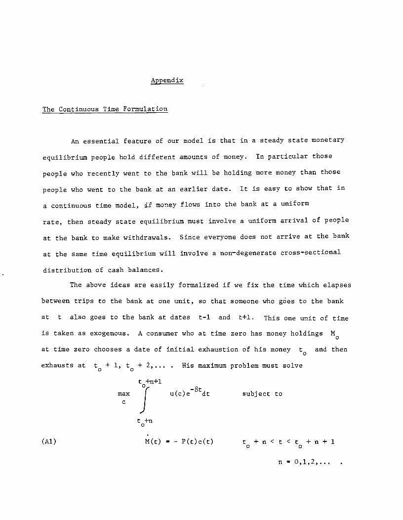
An essential feature of our model is that in a steady state monetary

equilibrium people hold different amounts of money, In particular those

people who recently went to the bank will be holding more money than those

people who went to the bank at an earlier date. It is easy to show that in

a continuous time model, if money flows into the bank at a uniform

rate, then steady state equilibrium must involve a uniform arrival of people

at the bank to make withdrawals. Since everyone does not arrive at the bank

at the same time equilibrium will involve a non—degenerate cross'-sectional

distribution of cash balances.

The above ideas are easily formalized if we fix the time which elapses

between trips to the bank at one unit, so that someone who g6es to the bank

at t also goes to the bank at dates t—l and t+l. This one unit of time

is taken as exogenous. A consumer who at time zero has money holdings M

at time zero chooses a date of initial exhaustion of his money to and then

exhausts at to + 1, to + 2 His maximum problem must solve

t +n+l

max u(c)etdt subject to

t +n0

(Al) M(t) = — P(t)c(t) t + n < t < t + n + 10 0

n = 0,1,2

A—2

(A2) M(t + n) = 0 n = 0,1,2,...,

(A3) M(t) > 0

and subject to a wealth constraint as in the text. Note that (Al) and

(A3) are equivalent to the Clower constraint, Eq. (A2) is the condition

that the consumer exhausts his money before arriving at the bank. In an

equilibrium model with positive nominal rates it is easy to derive (A2) as

an optimal policy for individuals.

It is convenient to assume logarithmic utility. In this case a

necessary condition for a consumer to be an optimum is that etP(t)c(t) is

a constant between trips to the bank. The constant is determined so that

the money withdrawn at t, M(t), exhausts at to + l Let M(t,t0) denote

the stock of money held at t [t,t+l.] of someone who goes to the bank

at to, Then the above two remarks imply:

— —(t—t)(A4) N(t,t ) = M(t )

— e

e—1Let MSdt be the size of the monetary injection which occurs via

an open market operation between t and t+dt, The stock of money flowing

into the bank between t and t+dt is composed of the monetary injectio-ir plus

spending flowing into stores MSdt + P(t)ydt, where P(t)ydt is the value

of spending during t to t+dt. Recall that output is fixed at a flow rate

of y and the supply of goods must equal the demand f or goods. Unless the

nominal interest rate is zero the money withdrawn from the bank during

the period x to x+dx must equal the stock which has flowed in:

A-3

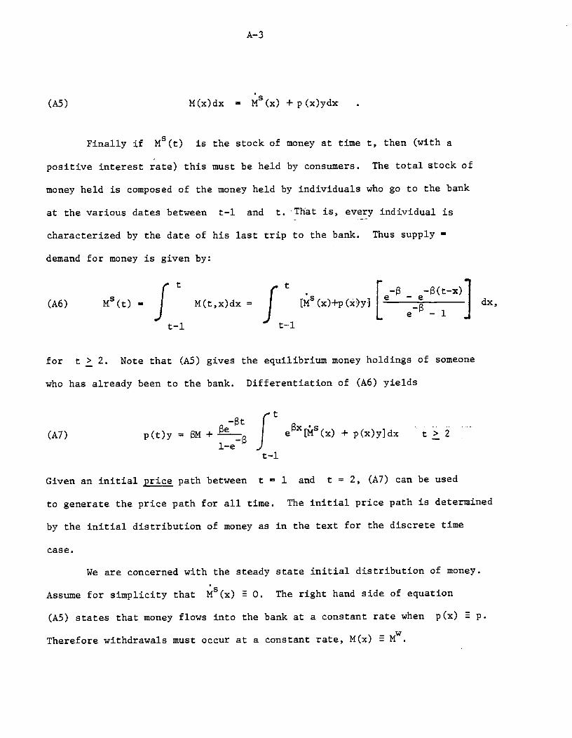
(A5) M(x)dx = MS(x) + p (x)ydx

Finally if MS(t) is the stock of money at time t, then (with a

positive interest rate) this must be held by consumers. The total stock of

money held is composed of the money held by individuals who go to the bank

at the various dates between t—l and t. That is, every individual is

characterized by the date of his last trip to the bank. Thus supply =

demand for money is given by:

(A6) MS(t) = f M(t,x)dx = f [M5(x)+p(*)y [e

(tx)] dx,

for t > 2. Note that (A5) gives the equilibrium money holdings of someone

who has already been to the bank. Differentiation of (A6) yields

(A7) p(t)y = + f e[(x) + p(x)yjdx t > 21

Given an initial price path between t = 1 and t 2, (A7) can be used

to generate the price path for all time. The initial price path Is determined

by the initial distribution of money as in the text for the discrete time

case.

We are concerned with the steady state initial distribution of money.

Assume for simplicity that M5(x) 0. The right hand side of equation

(A5) states that money flows into the bank at a constant rate when p(x) p.

Therefore withdrawals must occur at a constant rate, M(x) MW.

A—4

A person who is x units of time from his last withdrawal has money holdings

given by (A4):

- -x(A8) M(x) M(t + x,t ) = MW

— e0 0 e —i

But this must give the initial distribution of cash balances in the steady

staten That is, there are a continuum of traders labelled by x C [0,1).

Person x must begin with cash equal to M(x), and person x will arrive at

the bank at t = l—x. This must be the case because we have shown that with

P(x) constant, M(x) is constant. Thus the arrival rate of people at the bank

must be uniform in time (since the money flowing in is time homogeneous).

Once we know that the arrival rate is uniform, (A8) gives the initial distri—

bution of money which would lead to a uniform arrival rate. Thus, as we noted in

the text it is not an equilibrium for everyone to hold the same amount of

money.