Ann. Geophys., 34, 1053–1068, 2016www.ann-geophys.net/34/1053/2016/doi:10.5194/angeo-34-1053-2016© Author(s) 2016. CC Attribution 3.0 License.

Latitudinal and longitudinal dependence of the cosmic ray diurnalanisotropy during 2001–2014Anastasia Tezari1,*, Helen Mavromichalaki1, Dimitrios Katsinis1, Anastasios Kanellakopoulos1, Sofia Kolovi1,Christina Plainaki2,1, and Maria Andriopoulou3

1Nuclear and Particle Physics Department, Faculty of Physics, National and Kapodistrian University of Athens,Zografos, 15784 Athens, Greece2INAF-IAPS, Via del Fosso del Cavaliere, 00133, Rome, Italy3Space Research Institute, Austrian Academy of Sciences, Graz, Austria* Invited contribution by A. Tezari, recipient of the EGU Outstanding Student Poster (OSP) Award 2015.

Correspondence to: Helen Mavromichalaki (emavromi@phys.uoa.gr)

Received: 4 July 2016 – Revised: 14 October 2016 – Accepted: 18 October 2016 – Published: 21 November 2016

Abstract. The diurnal anisotropy of cosmic ray intensity forthe time period 2001 to 2014 is studied, covering the maxi-mum and the descending phase of solar cycle 23, the min-imum between solar cycles 23 and 24, and the ascendingphase and maximum of solar cycle 24. Cosmic ray intensitydata from 11 neutron monitor stations located at differentplaces around the Northern Hemisphere obtained from thehigh-resolution Neutron Monitor Database (NMDB) wereused. Special software was developed for the calculations ofthe amplitude and the phase of the diurnal anisotropy vectorson annual and monthly basis using Fourier analysis and forthe creation of the harmonic dial diagrams. The geomagneticbending for each station was taken into account in our calcu-lations determined from the asymptotic cones of each stationvia the Tsyganenko96 (Tsyganenko and Stern, 1996) mag-netospheric model. From our analysis, it was resulted thatthere is a different behavior of the diurnal anisotropy vectorsduring the different phases of the solar cycles depending onthe solar magnetic field polarity. The latitudinal and longi-tudinal distribution of the cosmic ray diurnal anisotropy wasalso examined by grouping the stations according to their ge-ographic coordinates, and it was shown that diurnal variationis modulated not only by the latitude but also by the longitudeof the stations. The diurnal anisotropy during strong eventsof solar and/or cosmic ray activity is discussed.

Keywords. Interplanetary physics (cosmic rays)

1 Introduction

The spatial anisotropy of the galactic cosmic radiation (GCR)in the interplanetary medium is observed as the daily vari-ation in cosmic ray (CR) intensity which is recorded byground-based detectors. A detector on Earth scans the en-tire sky during a time period of 24 h, since the Earth com-pletes one rotation around its own axis once in this timerange (Singh et al., 2013). Consequently, the detectors scanthrough different portions of the CR angular distribution witha 1-day period. The projection of this anisotropy on the eclip-tic plane may be observed as diurnal anisotropy (Yeeramand Saengdokmai, 2015). As a result, the intensity of GCRrecorded by ground-based neutron monitors (NMs) showsperiodic and abrupt changes as a function of space, time,and energy (Oh et al., 2010). This phenomenon, which isknown as the diurnal anisotropy of CR intensity, is a local-time short-term variation (Pomerantz and Duggal, 1971;Ahluwalia, 1988).

The diurnal variation is due to complex phenomena,deriving from the convective–diffusive theory, which in-volves the radial convection of GCR flux by the solar windand the inward diffusion along the interplanetary magneticfield (IMF) (Parker, 1964; Rao, 1972; Forman and Gleeson,1975; Sabbah, 2013). An energy-independent anisotropicflow of CR particles in the 18 h co-rotational direction is gen-erated due to the equilibrium between the convection and dif-fusion mechanisms (Krymsky, 1964; Rao, 1972; Mishra andMishra, 2008). This can explain the long-term average, but

Published by Copernicus Publications on behalf of the European Geosciences Union.

1054 A. Tezari et al.: Latitudinal and longitudinal dependence of the cosmic ray diurnal anisotropy

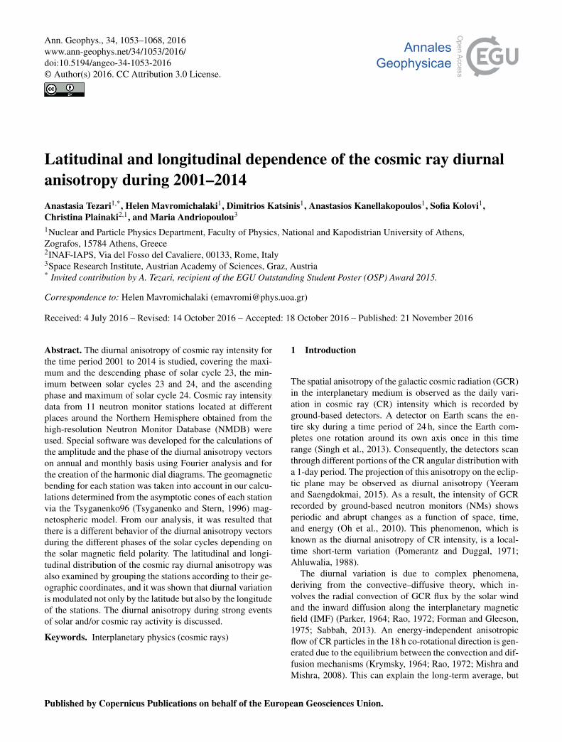
Figure 1. A map giving the geographic locations of the NM stations used in this work. The grouped stations are indicated by the same color.

not short-term variations in diurnal anisotropy (Yeeram andSaengdokmai, 2015). The diurnal anisotropy is also modu-lated by the geographic coordinates and the altitude of the de-tectors’ location on Earth (Mailyan and Chilingarian, 2010).

The diurnal amplitude follows the 11-year variation in thesolar cycle (SC) (Bieber and Chen, 1991; Tiwari et al., 2012),while the diurnal phase probably displays a correlation withthe magnetic solar cycle (22-year variation). This is due tothe reversal of the solar magnetic field (SMF) around solarmaximum activity (Ahluwalia, 1988). Consequently, a sig-nificant variability of the diurnal anisotropy vector is ob-served in terms of amplitude and time of maximum, whenconsidered on a SC variation basis (Mishra and Mishra,2005). The average diurnal amplitude was calculated on theorder of 0.6 % but sometimes can be as great as 1.5 % (For-man and Gleeson, 1975). The continually changing condi-tions in the interplanetary space cause a large day-to-dayvariability in the solar diurnal variation in CR intensity. Phe-nomena related to solar and CR variations may also be affect-ing the diurnal anisotropy. Such phenomena include ground-level enhancements (GLEs), Forbush decreases (FDs) andmagnetospheric effects (MEs), which are not interpretedin the same way by every NM (Burlaga and Ness, 1998;Plainaki et al., 2007, 2014). The characteristics of diurnalanisotropy show a remarkable variation during these extremeevents (Tezari and Mavromichalaki, 2016).

In this work the diurnal anisotropy of the CR intensityrecorded at selected NM stations of the worldwide neu-tron monitor network, located in the Northern Hemisphere,with different geographic coordinates and threshold rigidityis studied. The stations are grouped according to their ge-ographic latitudes and longitudes, taking into account theirasymptotic cones of viewing. The amplitude and the time ofmaximum of the CR diurnal anisotropy vectors during the

different phases of SCs 23 and 24 and during intense CRevents are examined and discussed.

2 Data analysis

Values of the CR intensity recorded at the NM stations ofApatity (APTY), Athens (ATHN), Jungfraujoch (JUNG),Irkutsk (IRKT), Kiel (KIEL), Lomnický štít (LMKS),Moscow (MOSC), Newark (NWRK), Novosibirsk (NVBK),Oulu (OULU), and Rome (ROME) that are hourly correctedfor pressure and efficiency have been used in this work.These data are obtained from the high-resolution NeutronMonitor Database (NMDB; http://www.nmdb.eu) or fromthe websites of each individual station. A list of these sta-tions with their characteristics such as the geographic coor-dinates, the altitude, the cut-off rigidity, and the geomagneticbending are given in Table 1. These stations are widely dis-tributed around the Northern Hemisphere and are separatedinto five groups in order to study the latitudinal distributionof the CR diurnal anisotropy (same geographic longitude), aswell as the longitudinal one (same geographic latitude). Thelocation of these NMs is indicated in the map of Fig. 1, withthe different colors corresponding to the different groups.These groups are GR 1 (shown in blue), including the sta-tions ATHN, LMKS, and OULU; GR 2 (green), includingthe stations JUNG, KIEL, and ROME; GR 3 (red), includ-ing the stations APTY and MOSC; GR 4 (orange), includ-ing the stations IRKT, KIEL, MOSC, NWRK, and NVBK;and GR 5 (purple), including the stations ATHN, ROME, andNWRK. The latitudinal distribution of CR intensity is stud-ied using the groups 1, 2, and 3 based on stations with almostthe same longitude and different latitude, while the longitu-dinal distribution with the groups 4 and 5 based on stationswith similar latitude and different longitude.

Ann. Geophys., 34, 1053–1068, 2016 www.ann-geophys.net/34/1053/2016/

A. Tezari et al.: Latitudinal and longitudinal dependence of the cosmic ray diurnal anisotropy 1055

Table 1. Characteristics of the NM stations used in this work.

NMs Type Geogr. lat. Geogr. long. Alt. (m) Rc (GV) Gb (h)

Apatity (APTY) 18NM64 67.57◦ N 33.4◦ E 181 0.65 2.16Oulu (OULU) 9NM64 65.05◦ N 25.47◦ E 15 0.81 2.27Kiel (KIEL) 18NM64 54.34◦ N 10.12◦ E 54 2.36 3.05Newark (NWRK) 9NM64 39.68◦ N 75.75◦W 50 2.40 3.51Moscow (MOSC) 24NM64 55.47◦ N 37.32◦ E 200 2.43 2.85Novosibirsk (NVBK) 24NM64 54.48◦ N 83.00◦ E 163 2.91 2.96Irkutsk (IRKT) 12NM64 52.47◦ N 104.03◦ E 2000 3.64 3.44Lomnický štít (LMKS) 8NM64 49.20◦ N 20.22◦ E 2634 3.84 3.58Jungfraujoch (JUNG) 3NM64 46.55◦ N 7.98◦ E 3570 4.50 3.94Rome (ROME) 20NM64 41.86◦ N 12.47◦ E 0 6.27 4.67Athens (ATHN) 6NM64 37.58◦ N 23.47◦ E 260 8.53 4.93

In the frame of this work a new Java-based software appli-cation, called the DIurnal Anisotropy Suite (DIAS), is pre-pared by the authors. DIAS enables the study and the calcu-lation of the amplitude and the time of maximum of the di-urnal anisotropy vectors of CR for every day and for a largenumber of days. This tool is capable of processing large datasets with a high level of automation. Various filters can beapplied in order to achieve higher data quality and eliminatethe effect of certain physical phenomena that are not usefulin our analysis. The selected filters used in this work are dis-cussed in the next paragraph and data are imported from .txtfiles with a special format provided by the users. The filtereddata can be presented on a harmonic dial and polar diagramsof monthly, annual, and multiannual diurnal anisotropy vec-tors can be generated automatically for a single station orgroup of stations. This allows the comparative study of theshort-term and long-term CR diurnal anisotropy. The graphsare generated automatically by Java software. This tool willbe soon available online on the web of the Athens NeutronMonitor Station (ANeMoS; http://cosray.phys.uoa.gr) withthe appropriate documentation.

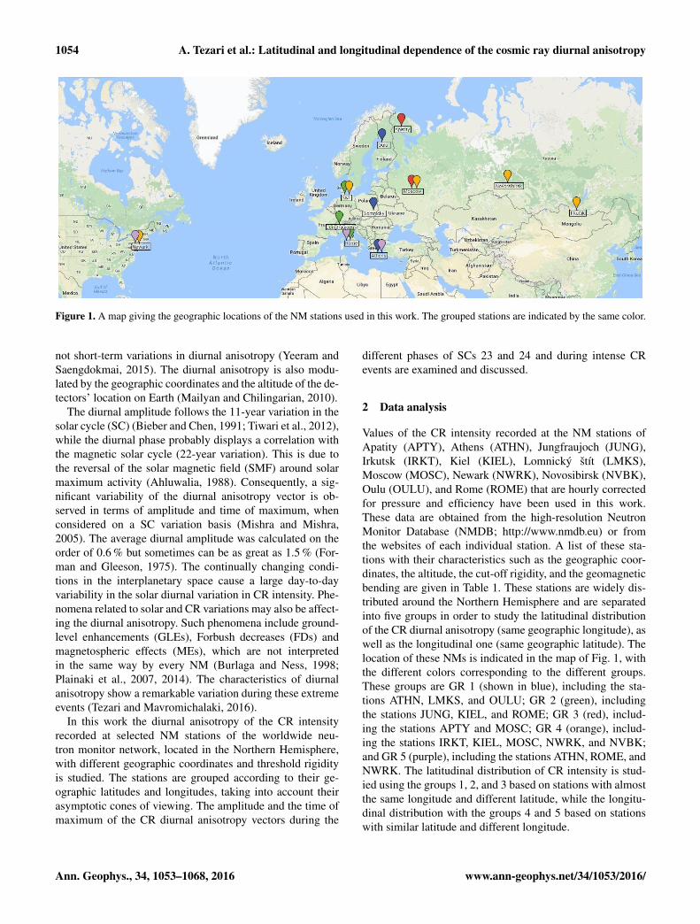
The hourly values of the CR intensity, which have beencorrected for pressure, have been normalized with respect ofthe mean value of the year 2001, which is the year of thesolar maximum and consequently the year of the cosmic rayminimum, and are presented in Fig. 2. We discard those daysthat exhibit an absolute value of the relative deviation of theaverage daily intensity with respect to the year 2001 that isgreater than 25 %. Furthermore, in order to eliminate majoreffects that may distort the long-term diurnal anisotropy, suchas GLEs and FDs, individual days with a difference betweenmaximum and minimum intensity greater than 5 % of theaverage daily intensity are also excluded (Bieber and Chen,1991; Kudela et al., 2008a). Days with gaps of more than 8 hare not used in this study (Yeeram and Saengdokmai, 2015).The average number of days per year used after the appliedfilters is approximately 361 for APTY, 351 for ATHN, 219for IRKT, 361 for JUNG, 339 for KIEL, 346 for LMKS, 359

Figure 2. Time profiles of the cosmic ray intensity normalized tothe mean value of the period 2001–2014 for all selected stations.

for MOSC, 360 for NWRK, 362 for NVBK, 361 for OULU,and 360 for ROME.

In order to plot the diurnal variation vectors, the diurnalanisotropy characteristics (amplitude and time of maximum)are calculated for each day using Fourier analysis accordingto the equation

Ii = f (ti)= Imean+A(cosωti +ϕ), (1)

where Imean represents the daily average of CR intensity,A the amplitude, ϕ the phase of diurnal variation, ω =2π

/24

(h−1) and i = 1,2, . . .24 (Firoz and Kudela, 2007;

www.ann-geophys.net/34/1053/2016/ Ann. Geophys., 34, 1053–1068, 2016

1056 A. Tezari et al.: Latitudinal and longitudinal dependence of the cosmic ray diurnal anisotropy

Firoz, 2008). Our data have been normalized according tothe equation

Ai =|Ii − Imean|

Imean100(%). (2)

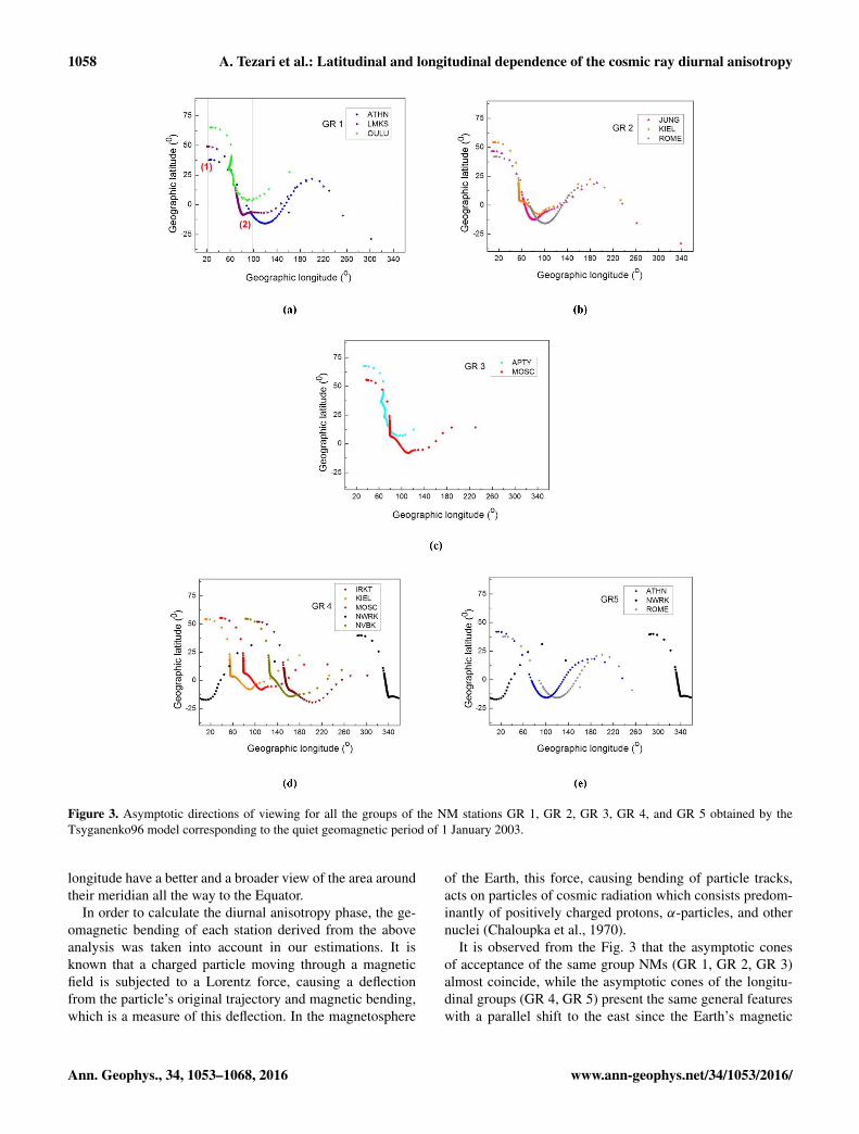
In order to calculate the time of maximum of the diur-nal anisotropy in local time (LT), a continuous study ofthe asymptotic cones of acceptance of the NMs was per-formed. The cones for all used NMs were calculated usingthe Tsyganenko96 magnetospheric model (Tsyganenko andStern, 1996). The asymptotic cones of acceptance for thefour groups of NM stations are calculated by using the ac-curate magnetic field data of 1 January 2003 correspondingto quiet geomagnetic conditions (Kp= 0, Dst= 0). Then thegeomagnetic bending value, Gb, for each NM was calculatedusing the asymptotic longitude of each NM (point 1) and cal-culating the angle between this point and the point presentingthe maximum CR flux (point 2) in the eastern direction (Hat-ton and Carswell, 1963; Shea et al., 1965). An example isgiven for the Athens NM in Fig. 3a. Thus, the equation forthe calculation of the diurnal phase in LT including the geo-magnetic bending correction for each station is given by thefollowing relation:

LT= UT+1T +Gb, (3)

where LT is the time of maximum in local time, UT is the cor-responding one in universal time, 1T is the transition timefrom UT to LT, and Gb is the correction for the geomagneticbending. More specifically, 1T is an integer parameter ex-pressed in hours and gives the difference of the time zonesof each station. The above equation can be written for eachstation as follows:

LTAPTY = UT+ 3+ 2.16 (h) LTNEWK = UT− 5+ 3.51 (h)LTOULU = UT+ 2+ 2.27 (h) LTLMKS = UT+ 1+ 3.58 (h)LTMOSC = UT+ 3+ 2.85 (h) LTJUNG = UT+ 1+ 3.94 (h) (4)LTNVBK = UT+ 6+ 2.96 (h) LTROME = UT+ 1+ 4.67 (h)LTKIEL = UT+ 1+ 3.05 (h) LTATHN = UT+ 2+ 4.93 (h)

LTIRKT = UT+ 8+ 3.44 (h).

Using the results of the geomagnetic study, the annual av-erage values of the amplitude and the time of maximum in LTand UT for all the NM stations are calculated and are givenin Table 2 (a, b, c). The calculated diurnal vectors of the cos-mic ray intensity according to Eqs. (1), (2), (3), and (4) forthe selected stations are presented on a harmonic dial on ayearly and monthly basis (Mavromichalaki, 1989; Tezari andMavromichalaki, 2016; Mavromichalaki et al., 2016) usingsimple vector calculus and the newly developed DIAS soft-ware. The length of the vector represents the diurnal ampli-tude, while the vector’s direction is equivalent to the time ofmaximum.

3 Geomagnetic bending

The asymptotic cone of acceptance of a NM is defined as thesolid angle of the asymptotic directions of approach of CRparticles of various energies outside the influence of the ge-omagnetic field and can contribute significantly to the count-ing rate of the detector (McCracken et al., 1968; Razdan andSummers, 1965; Mishra and Mishra, 2008). The diurnal vari-ation in the CR intensity at high-latitude stations, where theasymptotic cones of approach scan the meridian, provides agood comprehension of the longitudinal distribution of theanisotropy averaged in time and latitudes according to theasymptotic trajectories (Dorman and Fischer, 1968). The ef-fective cut-off rigidities of the NMs have been taken into ac-count for the calculation of the geomagnetic bending (Storiniet al., 1999). The effect of the geomagnetic field on the par-ticle trajectories is of great importance for the study of thediurnal anisotropy of CR intensity as it may affect the diur-nal amplitude.

In the current analysis, the asymptotic directions of view-ing for the NMs are calculated using the Tsyganenko96magnetospheric model (Tsyganenko, 1989, 1995; Tsyga-nenko and Stern, 1996; Belov et al., 2005), which is a semi-empirical best-fit representation of the Earth’s magnetic field,based on a large satellite observations data sets. Using differ-ent field models, especially during geomagnetic disturbancesor GLEs (studied in the context of diurnal wave in Sect. 4.3),may lead to different transmissivity of CR (Kudela et al.,2008b; Desorgher et al., 2009).

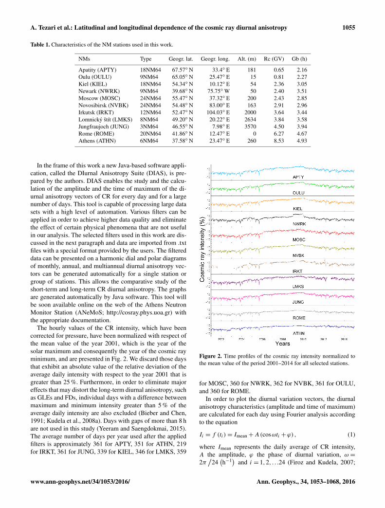
The term “NM asymptotic cone” is used to define the set ofallowed trajectory traces, as expected by the Stormer theory.In the current paper, we perform calculations in order to de-rive the intersections of the allowed particle trajectories withthe atmospheric layer at the altitude of 80 km (for a descrip-tion of the applied method see Plainaki et al., 2007, 2009).Since each trajectory corresponds to a different energy (rigid-ity), we obtain for each NM station a set of allowed posi-tions defined by latitude–longitude pair values. The magne-tospheric windows for all NMs used in this work are definedand presented in Fig. 3a, b, c, d, and e. For all the groupsof stations, each point refers to the axis of the cone (as it isfor particles arriving vertically) and to a particular rigidity.There is a variation step depending on the particle energy;therefore, each point of the diagram from west to east direc-tion corresponds to a different particle rigidity, beginning at999 GV (which is the energy of a particle detected at the sta-tion). From 18.00 to 0.80 GV the step is constant (0.20 GV).It is observed that the asymptotic cones have as a startingpoint the given NM and unfold with direction towards theEquator. The closer to the Equator a station is, the larger thepart of its cone spiraling around the Equator is. This effect of-fers better and broader view (geographical latitude-wise) ofthe ecliptic plane due to the high value of magnetic rigidityin such areas. On the other hand, NMs of high geographical

Ann. Geophys., 34, 1053–1068, 2016 www.ann-geophys.net/34/1053/2016/

A. Tezari et al.: Latitudinal and longitudinal dependence of the cosmic ray diurnal anisotropy 1057

Table 2. Mean annual values of (a) the normalized diurnal amplitude, (b) the time of maximum in UT, and (c) the time of maximum in LTof cosmic ray intensity recorded at the selected NM stations for the time period 2001–2014.

(a) Yearly diurnal amplitude (%)

YEAR APTY OULU KIEL NWRK MOSC NVBK IRKT LMKS JUNG ROME ATHN

2001 0.84 0.90 0.82 0.95 0.81 0.91 0.86 0.85 0.93 0.79 0.892002 0.79 0.89 0.82 0.93 0.81 0.88 0.89 0.87 0.95 0.78 0.912003 0.73 0.83 0.77 0.89 0.74 0.77 0.79 0.80 0.90 0.75 0.922004 0.71 0.80 0.75 0.87 0.75 0.76 0.80 0.80 0.84 0.72 0.862005 0.76 0.87 0.79 0.89 0.78 0.80 0.67 0.80 0.87 0.72 0.982006 0.66 0.76 0.71 0.76 0.65 0.72 0.60 0.70 0.77 0.62 0.842007 0.62 0.69 0.66 0.72 0.60 0.66 0.54 0.65 0.72 0.58 0.792008 0.58 0.65 0.77 0.66 0.57 0.62 0.48 0.59 0.68 0.54 0.762009 0.53 0.62 0.83 0.62 0.52 0.56 0.60 0.54 0.65 0.54 0.712010 0.63 0.75 1.43 0.72 0.64 0.66 0.71 0.66 0.75 0.59 0.822011 0.73 0.80 0.92 0.83 0.73 0.75 0.82 0.78 0.83 0.68 0.882012 0.74 0.85 0.96 0.88 0.78 0.78 0.73 0.94 0.90 0.70 1.002013 0.72 0.81 0.90 0.85 0.71 0.73 0.69 0.84 0.83 0.65 0.872014 0.71 0.79 0.85 0.84 0.69 0.74 0.86 0.73 0.83 0.66 0.86

(b) Yearly diurnal phase (UT)

2001 12.30 12.97 13.14 15.72 12.45 10.55 10.57 13.26 12.81 12.45 11.002002 12.57 12.88 13.18 14.86 12.59 10.37 9.98 12.93 12.78 12.59 11.562003 12.41 13.05 13.33 15.11 12.84 9.97 9.13 13.06 12.95 12.84 12.862004 12.45 12.89 12.81 16.17 12.36 9.04 9.00 13.07 13.10 12.36 12.362005 12.44 13.15 13.05 16.30 12.32 10.07 7.74 13.05 12.93 12.32 13.142006 12.41 12.88 13.02 16.03 12.31 9.24 7.81 12.73 12.21 12.31 11.592007 12.07 13.20 12.94 15.95 12.24 8.91 8.14 12.60 12.74 12.24 12.442008 12.18 12.60 12.74 15.23 12.05 8.92 8.52 12.65 12.55 12.05 12.322009 12.26 12.08 12.90 14.83 11.55 8.81 8.14 12.89 12.38 11.55 12.202010 12.47 12.49 12.54 15.24 12.35 9.83 9.80 12.92 12.66 12.35 11.822011 13.09 13.08 12.50 15.14 12.86 10.78 8.88 13.00 13.23 12.86 12.472012 12.87 12.83 12.42 15.53 12.13 10.67 8.94 12.03 12.56 12.13 12.022013 12.63 12.51 12.17 14.88 12.59 9.71 9.22 12.53 12.92 12.59 11.552014 12.10 12.14 11.88 14.48 11.42 9.63 10.57 11.94 12.16 11.42 11.67

(c) Yearly diurnal phase (LT)

2001 17.46 17.24 17.19 15.23 18.14 19.51 22.01 17.84 17.75 18.12 17.932002 17.73 17.15 17.23 14.37 17.94 19.33 21.42 17.51 17.72 18.26 18.492003 17.57 17.32 17.38 14.62 17.92 18.93 20.57 17.64 17.89 18.51 19.792004 17.61 17.16 16.86 15.68 17.79 18.00 20.44 17.65 18.04 18.03 19.292005 17.60 17.42 17.10 15.81 17.74 19.03 19.18 17.63 17.87 17.99 20.072006 17.57 17.15 17.07 15.54 17.13 18.20 19.25 17.31 17.15 17.98 18.522007 17.23 17.47 16.99 15.46 16.99 17.87 19.58 17.18 17.68 17.91 19.372008 17.34 16.87 16.79 14.74 16.68 17.88 19.96 17.23 17.49 17.72 19.252009 17.42 16.35 16.95 14.34 16.67 17.77 19.58 17.47 17.32 17.22 19.132010 17.63 16.76 16.59 14.75 16.92 18.79 21.24 17.50 17.60 18.02 18.752011 18.25 17.35 16.55 14.65 18.09 19.74 20.32 17.58 18.17 18.53 19.402012 18.03 17.10 16.47 15.04 17.74 19.63 20.38 16.61 17.50 17.80 18.952013 17.79 16.78 16.22 14.39 17.79 18.67 20.66 17.11 17.86 18.26 18.482014 17.26 16.41 15.93 13.99 17.11 18.59 22.01 16.52 17.10 17.09 18.60

www.ann-geophys.net/34/1053/2016/ Ann. Geophys., 34, 1053–1068, 2016

1058 A. Tezari et al.: Latitudinal and longitudinal dependence of the cosmic ray diurnal anisotropy

Figure 3. Asymptotic directions of viewing for all the groups of the NM stations GR 1, GR 2, GR 3, GR 4, and GR 5 obtained by theTsyganenko96 model corresponding to the quiet geomagnetic period of 1 January 2003.

longitude have a better and a broader view of the area aroundtheir meridian all the way to the Equator.

In order to calculate the diurnal anisotropy phase, the ge-omagnetic bending of each station derived from the aboveanalysis was taken into account in our estimations. It isknown that a charged particle moving through a magneticfield is subjected to a Lorentz force, causing a deflectionfrom the particle’s original trajectory and magnetic bending,which is a measure of this deflection. In the magnetosphere

of the Earth, this force, causing bending of particle tracks,acts on particles of cosmic radiation which consists predom-inantly of positively charged protons, α-particles, and othernuclei (Chaloupka et al., 1970).

It is observed from the Fig. 3 that the asymptotic conesof acceptance of the same group NMs (GR 1, GR 2, GR 3)almost coincide, while the asymptotic cones of the longitu-dinal groups (GR 4, GR 5) present the same general featureswith a parallel shift to the east since the Earth’s magnetic

Ann. Geophys., 34, 1053–1068, 2016 www.ann-geophys.net/34/1053/2016/

A. Tezari et al.: Latitudinal and longitudinal dependence of the cosmic ray diurnal anisotropy 1059

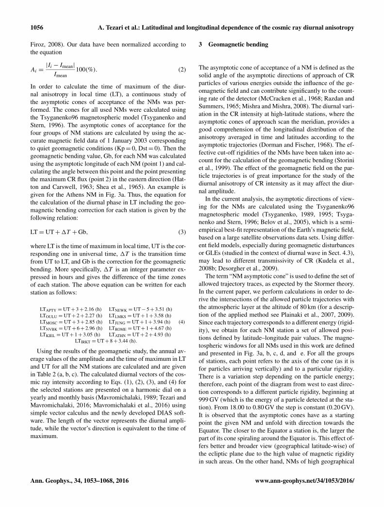
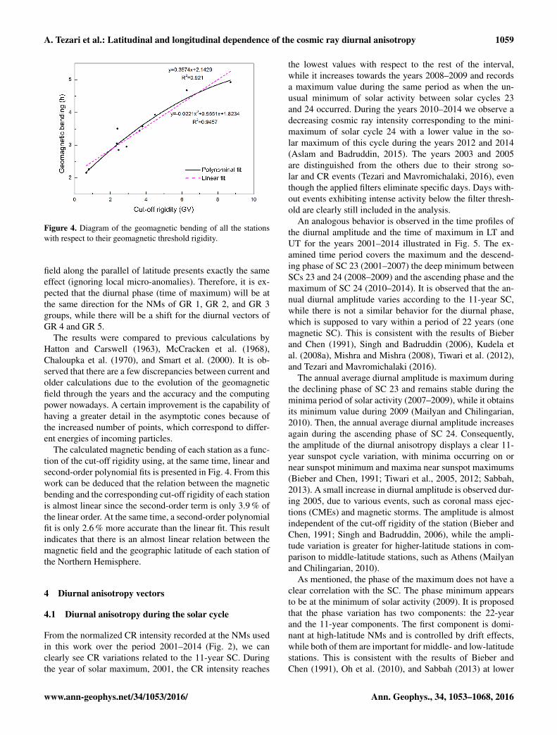
Figure 4. Diagram of the geomagnetic bending of all the stationswith respect to their geomagnetic threshold rigidity.

field along the parallel of latitude presents exactly the sameeffect (ignoring local micro-anomalies). Therefore, it is ex-pected that the diurnal phase (time of maximum) will be atthe same direction for the NMs of GR 1, GR 2, and GR 3groups, while there will be a shift for the diurnal vectors ofGR 4 and GR 5.

The results were compared to previous calculations byHatton and Carswell (1963), McCracken et al. (1968),Chaloupka et al. (1970), and Smart et al. (2000). It is ob-served that there are a few discrepancies between current andolder calculations due to the evolution of the geomagneticfield through the years and the accuracy and the computingpower nowadays. A certain improvement is the capability ofhaving a greater detail in the asymptotic cones because ofthe increased number of points, which correspond to differ-ent energies of incoming particles.

The calculated magnetic bending of each station as a func-tion of the cut-off rigidity using, at the same time, linear andsecond-order polynomial fits is presented in Fig. 4. From thiswork can be deduced that the relation between the magneticbending and the corresponding cut-off rigidity of each stationis almost linear since the second-order term is only 3.9 % ofthe linear order. At the same time, a second-order polynomialfit is only 2.6 % more accurate than the linear fit. This resultindicates that there is an almost linear relation between themagnetic field and the geographic latitude of each station ofthe Northern Hemisphere.

4 Diurnal anisotropy vectors

4.1 Diurnal anisotropy during the solar cycle

From the normalized CR intensity recorded at the NMs usedin this work over the period 2001–2014 (Fig. 2), we canclearly see CR variations related to the 11-year SC. Duringthe year of solar maximum, 2001, the CR intensity reaches

the lowest values with respect to the rest of the interval,while it increases towards the years 2008–2009 and recordsa maximum value during the same period as when the un-usual minimum of solar activity between solar cycles 23and 24 occurred. During the years 2010–2014 we observe adecreasing cosmic ray intensity corresponding to the mini-maximum of solar cycle 24 with a lower value in the so-lar maximum of this cycle during the years 2012 and 2014(Aslam and Badruddin, 2015). The years 2003 and 2005are distinguished from the others due to their strong so-lar and CR events (Tezari and Mavromichalaki, 2016), eventhough the applied filters eliminate specific days. Days with-out events exhibiting intense activity below the filter thresh-old are clearly still included in the analysis.

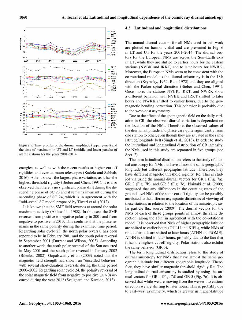
An analogous behavior is observed in the time profiles ofthe diurnal amplitude and the time of maximum in LT andUT for the years 2001–2014 illustrated in Fig. 5. The ex-amined time period covers the maximum and the descend-ing phase of SC 23 (2001–2007) the deep minimum betweenSCs 23 and 24 (2008–2009) and the ascending phase and themaximum of SC 24 (2010–2014). It is observed that the an-nual diurnal amplitude varies according to the 11-year SC,while there is not a similar behavior for the diurnal phase,which is supposed to vary within a period of 22 years (onemagnetic SC). This is consistent with the results of Bieberand Chen (1991), Singh and Badruddin (2006), Kudela etal. (2008a), Mishra and Mishra (2008), Tiwari et al. (2012),and Tezari and Mavromichalaki (2016).

The annual average diurnal amplitude is maximum duringthe declining phase of SC 23 and remains stable during theminima period of solar activity (2007–2009), while it obtainsits minimum value during 2009 (Mailyan and Chilingarian,2010). Then, the annual average diurnal amplitude increasesagain during the ascending phase of SC 24. Consequently,the amplitude of the diurnal anisotropy displays a clear 11-year sunspot cycle variation, with minima occurring on ornear sunspot minimum and maxima near sunspot maximums(Bieber and Chen, 1991; Tiwari et al., 2005, 2012; Sabbah,2013). A small increase in diurnal amplitude is observed dur-ing 2005, due to various events, such as coronal mass ejec-tions (CMEs) and magnetic storms. The amplitude is almostindependent of the cut-off rigidity of the station (Bieber andChen, 1991; Singh and Badruddin, 2006), while the ampli-tude variation is greater for higher-latitude stations in com-parison to middle-latitude stations, such as Athens (Mailyanand Chilingarian, 2010).

As mentioned, the phase of the maximum does not have aclear correlation with the SC. The phase minimum appearsto be at the minimum of solar activity (2009). It is proposedthat the phase variation has two components: the 22-yearand the 11-year components. The first component is domi-nant at high-latitude NMs and is controlled by drift effects,while both of them are important for middle- and low-latitudestations. This is consistent with the results of Bieber andChen (1991), Oh et al. (2010), and Sabbah (2013) at lower

www.ann-geophys.net/34/1053/2016/ Ann. Geophys., 34, 1053–1068, 2016

1060 A. Tezari et al.: Latitudinal and longitudinal dependence of the cosmic ray diurnal anisotropy

Figure 5. Time profiles of the diurnal amplitude (upper panel) andthe time of maximum in UT and LT (middle and lower panels) ofall the stations for the years 2001–2014.

energies, as well as with the recent results at higher cut-offrigidities and even at muon telescopes (Kudela and Sabbah,2016). Athens shows the largest phase variation, as it has thehighest threshold rigidity (Bieber and Chen, 1991). It is alsoobserved that there is no significant phase shift during the de-scending phase of SC 23 and it remains invariant during theascending phase of SC 24, which is in agreement with the“odd–even” SC model proposed by Tiwari et al. (2012).

It is known that the SMF field reverses at around the solarmaximum activity (Ahluwalia, 1988). In this case the SMFreverses from positive to negative polarity in 2001 and fromnegative to positive in 2013. This confirms that the phase re-mains in the same polarity during the examined time period.Regarding solar cycle 23, the north polar reversal has beenreported to be in February 2001 and the south polar reversalin September 2001 (Durrant and Wilson, 2003). Accordingto another work, the north polar reversal of the Sun occurredin May 2001 and the south polar reversal in January 2002(Bilenko, 2002). Gopalswamy et al. (2003) noted that themagnetic field strength had shown an “unsettled behavior”with several short-duration reversals during the time period2000–2002. Regarding solar cycle 24, the polarity reversal ofthe solar magnetic field from negative to positive (A> 0) oc-curred during the year 2012 (Svalgaard and Kamide, 2013).

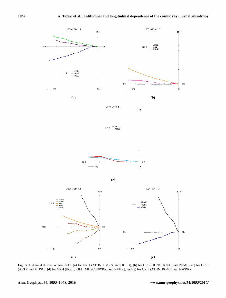
4.2 Latitudinal and longitudinal distributions

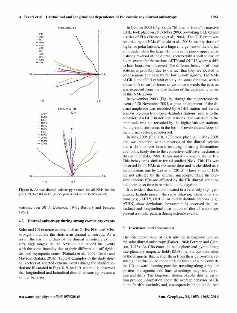
The annual diurnal vectors for all NMs used in this workare plotted on harmonic dial and are presented in Fig. 6in LT and UT for the years 2001–2014. The diurnal vec-tors for the European NMs are across the Sun–Earth axisin UT, while they are shifted to earlier hours for the easternstations (NVBK and IRKT) and to later hours for NWRK.Moreover, the European NMs seem to be consistent with theco-rotational model, as the diurnal anisotropy is in the 18 hdirection (Krymsky, 1964; Rao, 1972) and they are alignedwith the Parker spiral direction (Bieber and Chen, 1991).Once more, the stations NVBK, IRKT, and NWRK showa different behavior with NVBK and IRKT shifted to laterhours and NWRK shifted to earlier hours, due to the geo-magnetic bending correction. This behavior is probably dueto the west–east asymmetry.

Due to the effect of the geomagnetic field on the daily vari-ation in CR, the observed diurnal variation is dependent onthe location of the NMs. Therefore, the observed values ofthe diurnal amplitude and phase vary quite significantly fromone station to other, even though they are situated in the samelatitude/longitude belt (Singh et al., 2013). In order to studythe latitudinal and longitudinal distribution of CR intensity,the NMs used in this study are separated in five groups (seeSect. 2).

The term latitudinal distribution refers to the study of diur-nal anisotropy for NMs that have almost the same geographiclongitude but different geographic latitude. Therefore, theyhave different magnetic threshold rigidity, Rc. This is stud-ied via using the annual diurnal vectors for GR 1 (Fig. 7a),GR 2 (Fig. 7b), and GR 3 (Fig. 7c). Plainaki et al. (2009)suggested that any differences in the counting rates of theground level NMs of the same cut-off rigidity can be possiblyattributed to the different asymptotic directions of viewing ofthese stations in relation to the location of the anisotropic so-lar particle flux source (2009). The diurnal vectors for theNMs of each of these groups points in almost the same di-rection, along the 18 h, in agreement with the co-rotationalmodel. It is observed that NMs of higher geographic latitudeare shifted to earlier hours (OULU and KIEL), while NMs ofmiddle latitude are shifted to later hours (ATHN and ROME).ATHN is shifted to later hours, probably due to the fact thatit has the highest cut-off rigidity. Polar stations also exhibitthe same behavior (GR 3).

The term longitudinal distribution refers to the study ofdiurnal anisotropy for NMs that have almost the same ge-ographic latitude but different geographic longitude. There-fore, they have similar magnetic threshold rigidity Rc. Thelongitudinal diurnal anisotropy is studied by using the an-nual vectors for GR 4 (Fig. 7d) and GR 5 (Fig. 7e). It is ob-served that while we are moving from the western to easterndirection we are shifting to later hours. This is probably dueto east–west asymmetry, which is greater in higher-latitude

Ann. Geophys., 34, 1053–1068, 2016 www.ann-geophys.net/34/1053/2016/

A. Tezari et al.: Latitudinal and longitudinal dependence of the cosmic ray diurnal anisotropy 1061

Figure 6. Annual diurnal anisotropy vectors for all NMs for theyears 2001–2014 in LT (upper panel) and in UT (lower panel).

stations, over 50◦ N (Johnson, 1941; Burbury and Fenton,1952).

4.3 Diurnal anisotropy during strong cosmic ray events

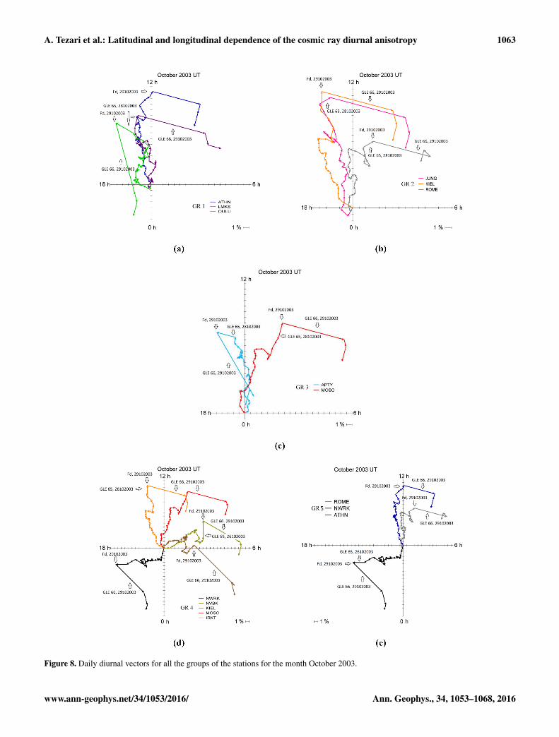
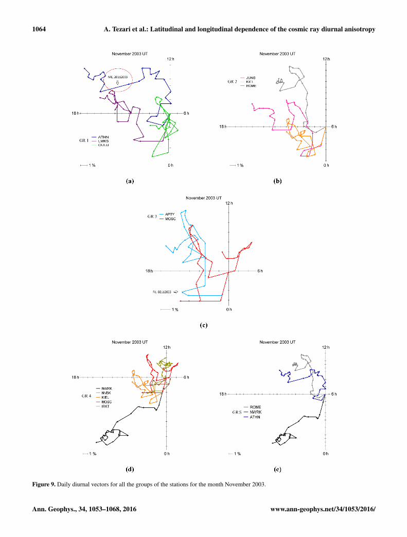
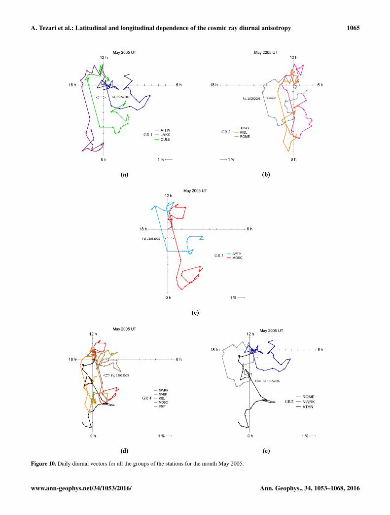
Solar and CR extreme events, such as GLEs, FDs, and MEs,strongly modulate the short-term diurnal anisotropy. As aresult, the harmonic dials of the diurnal anisotropy exhibitvery high ranges, as the NMs do not record the eventswith the same intensity due to their different cut-off rigidi-ties and asymptotic cones (Plainaki et al., 2009; Tezari andMavromichalaki, 2016). Typical examples of the daily diur-nal vectors of selected extreme events during the studied pe-riod are illustrated in Figs. 8, 9, and 10, where it is observedthat longitudinal and latitudinal diurnal anisotropy present asimilar behavior.

In October 2003 (Fig. 8), the “Mother of Halos”, a massiveCME, took place on 28 October 2003, provoking GLE 65 anda series of FDs (Eroshenko et al., 2004). The GLE event wasrecorded by all NMs (Plainaki et al., 2005), mainly those ofhigher or polar latitude, as a huge enlargement of the diurnalamplitude, while the large FD in the same period appeared asa strong reversal of the diurnal vectors with a shift to earlierhours, except for the stations APTY and OULU, where a shiftto later hours was observed. The different behavior of thesestations is probably due to the fact that they are located inpolar regions and have by far low cut-off rigidity. The NMsof GR 4 and GR 5 exhibit exactly the same variation, with aphase shift to earlier hours as we move towards the east, aswas expected from the distribution of the asymptotic conesof this NMs group.

In November 2003 (Fig. 9), during the magnetosphericevent of 20 November 2003, a great enlargement of the di-urnal amplitude was recorded by ATHN station and aurorawas visible even from lower-latitudes stations, similar to thebehavior of a GLE in northern stations. The variation in theamplitude was not recorded by the higher-latitude stations,but a great disturbance, in the form of reversals and loops ofthe diurnal vectors, is observed.

In May 2005 (Fig. 10), a FD took place in 11 May 2005and was recorded with a reversal of the diurnal vectorsand a shift to later hours, resulting in strong fluctuationsand loops, likely due to the convective–diffusive mechanism(Mavromichalaki, 1989; Tezari and Mavromichalaki, 2016).This behavior is similar for all studied NMs. This FD wasobserved in all NMs at the same time and is classified as asimultaneous one by Lee et al. (2015). These kinds of FDsare not affected by the diurnal anisotropy, while the non-simultaneous FDs are affected by the CR diurnal variationand their onset time is restricted to the daytime.

It is evident that stations located in a relatively high geo-graphic latitude present the same behavior, while polar sta-tions (e.g., APTY, OULU) or middle-latitude stations (e.g.,ATHN) show deviations; however, it is observed that lat-itudinal and longitudinal distribution of diurnal anisotropypresent a similar pattern during extreme events.

5 Discussion and conclusions

The solar modulation of GCR into the heliosphere inducesthe solar diurnal anisotropy (Parker, 1964; Forman and Glee-son, 1975). As CRs enter the heliosphere and gyrate alonginterplanetary magnetic field (IMF) line, various anomaliesof the magnetic flux scatter them from their gyro-orbits, re-sulting in diffusion. At the same time the solar wind convertsthe CR outward, causing particles traveling along a regularportion of magnetic field lines to undergo magnetic curva-ture and drifts. The long-term studies of solar diurnal varia-tion provide information about the average behavior of CRat the Earth’s proximity and, consequently, about the diurnal

www.ann-geophys.net/34/1053/2016/ Ann. Geophys., 34, 1053–1068, 2016

1062 A. Tezari et al.: Latitudinal and longitudinal dependence of the cosmic ray diurnal anisotropy

Figure 7. Annual diurnal vectors in LT (a) for GR 1 (ATHN, LMKS, and OULU), (b) for GR 2 (JUNG, KIEL, and ROME), (c) for GR 3(APTY and MOSC), (d) for GR 4 (IRKT, KIEL, MOSC, NWRK, and NVBK), and (e) for GR 5 (ATHN, ROME, and NWRK).

Ann. Geophys., 34, 1053–1068, 2016 www.ann-geophys.net/34/1053/2016/

A. Tezari et al.: Latitudinal and longitudinal dependence of the cosmic ray diurnal anisotropy 1063

Figure 8. Daily diurnal vectors for all the groups of the stations for the month October 2003.

www.ann-geophys.net/34/1053/2016/ Ann. Geophys., 34, 1053–1068, 2016

1064 A. Tezari et al.: Latitudinal and longitudinal dependence of the cosmic ray diurnal anisotropy

Figure 9. Daily diurnal vectors for all the groups of the stations for the month November 2003.

Ann. Geophys., 34, 1053–1068, 2016 www.ann-geophys.net/34/1053/2016/

A. Tezari et al.: Latitudinal and longitudinal dependence of the cosmic ray diurnal anisotropy 1065

Figure 10. Daily diurnal vectors for all the groups of the stations for the month May 2005.

www.ann-geophys.net/34/1053/2016/ Ann. Geophys., 34, 1053–1068, 2016

1066 A. Tezari et al.: Latitudinal and longitudinal dependence of the cosmic ray diurnal anisotropy

anisotropy observed by ground-based monitors. This infor-mation may be useful for better understanding of the mod-ulation processes (Venkatesan and Badruddin, 1990; Hall etal., 1996).

The asymptotic directions of viewing of the ground-basedNMs are determined by the configuration of the magneto-sphere and so they are sensitive to the time of day, to thetime of year, and to the level of the magnetic disturbances.The distortion of the geomagnetic field by the solar windmay cause a variation in the viewing direction at a speci-fied energy according to the local daytime. The diurnal am-plitude is affected by the asymptotic latitude of primary CRarrival, while the diurnal phase is influenced by the asymp-totic longitude for a specific solar diurnal variation (Humbleand Duldig, 2003). Therefore, the study of asymptotic conesof viewing is necessary in the analysis of diurnal anisotropy.Other effects, such as sidereal variations, are considered neg-ligible for long-term studies.

In this work, the characteristics of the CR diurnalanisotropy for 11 NMs during the years 2001 to 2014; cov-ering a complete SC, are studied. As the diurnal anisotropyis a phenomenon of local time, the study of the asymptoticcones of acceptance of the NMs is very important for the de-termination of the correction due to the geomagnetic bend-ing. A detailed study of both longitudinal and latitudinal dis-tribution of the diurnal anisotropy is performed for the firsttime and supports the idea that the behavior of the diurnalanisotropy of CR intensity is determined not by the magneticthreshold rigidity but actually by a combination of this andthe geographic coordinates of the given NM station.

The main results of this study can be summarized as fol-lows:

– The use of the geomagnetic bending and the updated ge-omagnetic field models (with external current systemssuch as Tsyganenko96), along with the developed soft-ware, leads to a better description of the diurnal charac-teristics for various geographic positions of NMs duringthe examined years 2001–2014, as well as for selectedtransitional events in the inner heliosphere.

– In order to have more accurate estimations of the diur-nal anisotropy characteristics, the asymptotic cones ofviewing for the examined NMs have been taken into ac-count and the geomagnetic bending for each station hasbeen calculated (Table 1) (Chaloupka et al., 1970; Hum-ble and Duldig, 2003)

– It was shown that the asymptotic cones of acceptanceare almost identical for each group of the latitudinaldistribution (GR 1, GR 2, GR 3), supporting the factthat the diurnal phase leads to the same direction. Onthe other hand, the asymptotic cones of the NMs of thelongitudinal distribution (GR 4) are shifted in parallel,resulting in a shift of the time of maximum.

– The annual average diurnal amplitude of the cosmic rayrecordings examined in this work follows the 11-yearvariation in the SC well, presenting a maximum valueduring the maximum periods of solar cycles 23 and 24(years 2001–2003 and 2012 respectively) and a mini-mum value during the solar minimum between the cy-cles 23 and 24 (year 2009). On the other hand, the di-urnal phase does not seem to present an analogous be-havior that is possibly extended to the 22-year magneticcycle (Bieber and Chen, 1991; Tiwari et al., 2012).

– During the examined period the diurnal anisotropy am-plitude of cosmic rays is almost identical for all NMs,while its variation is greater for the NMs located inhigh and polar geographic latitudes in comparison to themiddle- and equatorial-latitude stations (Table 2).

– We found a phase shift of the time of maximum to laterhours during the examined time period in the stationswith increasing cut-off rigidity with the greatest one ob-served in the Athens NM (cut-off rigidity 8.53 GV).

– It is concluded that the asymptotic latitude and theasymptotic longitude of the primary CR arrival affectthe diurnal amplitude and the diurnal time of maximum,respectively, for a given solar diurnal anisotropy (Hum-ble and Duldig, 2003). The variations in asymptotic di-rections during the day do not have a great influence onthe diurnal variation observed at the NMs, as the solardiurnal anisotropy is weakly rigidity-dependent.

– There is no evidence for a systematic phase shift of theyearly time of maximum of the diurnal anisotropy ofall stations for the examined period. This is because theperiod under study is characterized by solar magneticfield of the same polarity (A< 0) (Gopalswamy, 2003).

– Our results on the yearly average diurnal time of max-imum for all the NMs are consistent with the co-rotational model, which sets the value of this parame-ter at around 18 h in LT (Parker, 1964). We found thatthe estimations corresponding to NVBK and IRKT sta-tions are shifted to later hours in LT, while the one corre-sponding to NWRK is shifted to earlier hours (Fig. 7d).The opposite behavior is observed in the case of thephase in UT. This different behavior of eastern andwestern NMs is probably due to the west–east asym-metry, which is evident for geographic latitudes greaterthan 50◦ N (Burbury and Fenton, 1952).

– Diurnal variation is an effect of convection and diffu-sion due to the steady outer GCR source, while it isalso due to transitional effects in the inner heliosphere.Therefore, the diurnal anisotropy of cosmic rays is alsoaffected on a short-term basis by intense cosmic rayevents, such as GLEs, FDs, and MEs, which are mod-ulated from the solar activity (Tezari and Mavromicha-laki, 2016).

Ann. Geophys., 34, 1053–1068, 2016 www.ann-geophys.net/34/1053/2016/

A. Tezari et al.: Latitudinal and longitudinal dependence of the cosmic ray diurnal anisotropy 1067

In summary, a new software application, called the DI-urnal Anisotropy Suite (DIAS) is introduced for the studyof the characteristics and the representation of the diurnalanisotropy vectors. The online function of DIAS, hopefullyavailable in the next years, will provide continuous diurnalvariation monitoring. The related results will be useful forlong- term space weather monitoring integrating current es-timations based on ground-based and satellite data and/ormodeling.

6 Data availability

Data can be found on the NMDB website (http://nmdb.eu)(NMDB, 2008). Additionally, many of the stations used inthis work provide their data online on their own websites.

Acknowledgements. The authors are grateful to our colleagues ofthe Neutron Monitor Stations used in this work for kindly provid-ing their CR data. We acknowledge the Neutron Monitor Database(www.nmdb.eu), founded under the European Union’s SeventhFramework Programme (contract no. 213007), for providing CRdata. Athens Neutron Monitor Station is supported by the SpecialResearch Account of Athens University (70/4/5803). Thanks aredue to K. Kudela of the Slovak Academy of Sciences for his impor-tant comments reviewing this work, M. A. Shea, and D. F. Smartof the USA Air Force Research Laboratory and E. Eroshenko andV. Yanke of the Russian Academy of Sciences for useful discus-sions. The authors express many thanks to the EGU 2015 GeneralAssembly Scientific Committee, where part of this work was pre-sented and A. Tezari received an Outstanding Student Poster Award.

The topical editor, M. Temmer, thanks the two anonymous ref-erees for help in evaluating this paper.

References

Ahluwalia, H. S.: The regimes of the east- west and the radialanisotropies of cosmic rays in the heliosphere, Planet. Space Sci.,36, 1451–1459, doi:10.1016/0032-0633(88)90010-4, 1988.

Aslam, O. P. M. and Badruddin: Study of the cosmic ray modulationduring the recent unusual minimum and the mini-maximum ofsolar cycle 24, Sol. Phys., 290, 2333–2353, doi:10.1007/s11207-015-0753-5, 2015.

Belov, A., Eroshenko, E., Mavromichalaki, H., Plainaki, C., andYanke, V.: Solar cosmic rays during the extremely high groundlevel enhancement on 23 February 1956, Ann. Geophys., 23,2281–2291, doi:10.5194/angeo-23-2281-2005, 2005.

Bieber, J. W. and Chen, J. L.: Cosmic ray diurnal anisotropy, 1936–88: Implications for drift and modulation theories, Astrophys. J.,372, 301–313, doi:10.1086/169976, 1991.

Bilenko, I. A.: Coronal holes and the solar polar field re-versal, Astron. Astrophys., 396, 657–666, doi:10.1051/0004-6361:20021412, 2002.

Burbury, D. W. P. and Fenton, K. B.: The High Latitude East-WestAsymmetry of Cosmic Rays, Australian J. Scient. Res. A, 5, 47–58, 1952.

Burlaga, L. F. and Ness, N. F.: Voyager Observations of the Mag-netic Field in the Distant Heliosphere, Space Science Rev., 83,105–121, doi:10.1023/A:1005025613036, 1998.

Chaloupka, P., Dubinský, J., Fischer, S., and Kowalski, T.: Geo-magnetic bending and effective angles of approach of the cos-mic rays for various stations, Czech. J. Phys. B, 20, 447–452,doi:10.1007/BF01698403, 1970.

Desorgher, L., Kudela, K., Flückiger, E., Butikofer, R., Storini, M.,and Kalegaev, V.: Comparison of Earth’s magnetospheric mag-netic field models in the context of cosmic ray physics, ActaGeophys., 57, 75–87, doi:10.2478/s11600-008-0065-3, 2009.

Dorman, L. I. and Fischer, S.: Diurnal cosmic ray variation with theinclusion of the geometrical effects and the asymptotic cones ofapproach, Can. J. Phys., 46, S809–S811, doi:10.1139/p68-356,1968.

Durrant, C. J. and Wilson, P. R.: Observations and simulations ofthe polar field reversals in cycle 23, Sol. Phys., 214, 23–39,doi:10.1023/A:1024042918007, 2003.

Eroshenko, E., Belov, A., Mavromichalaki, H., Mariatos, G.,Oleneva, V., Plainaki, C., and Yanke, V.: Cosmic ray variationsduring the two great bursts of solar activity in the 23rd solar cy-cle, Sol. Phys., 224, 345–358, 2004.

Firoz, K. A.: On cosmic ray diurnal variations: disturbed andquiet days, Proc. WDS’8 Part 2, 183–188, ISBN-13: 978-80-7378-066-1, 2008.

Firoz, K. A. and Kudela, K.: Cosmic Rays and Low Energy ParticleFluxes Proc. WDS‘8 Part 2, 106–110, ISBN-13: 978-80-7378-024-1, 2007.

Forman, M. A. and Gleeson, L. F.: Cosmic ray stream-ing and anisotropies, Astrophys. Space Sci., 32, 77–94,doi:10.1007/BF00646218, 1975.

Gopalswamy, N., Lara, A., Yashiro, S., and Howard, A. R.: Coro-nal mass ejections and solar polarity reversal, Astrophys. J., 598,L63–L66, 2003.

Hall, D. L., Duldig, M. L., and Humble, J. E.: Analyses of siderealand solar anisotropies of cosmic rays, Space Sci. Rev., 78, 401–442, doi:10.1007/BF00171926, 1996.

Hatton, C. J. and Carswell, D. A.: Asymptotic directions of ap-proach of vertically incident cosmic rays for 85 neutron moni-tor stations, Deep River Laboratory, Atomic Energy of CanadaLimited-1824, Chalk River, Ontario, 1963.

Humble, J. E. and Duldig, M. L.: The Effect of Variable Directionsof Viewing on the Interpretation of Diurnal Variations observedby Neutron Monitors, Proc. 28th ICRC 2003, 4197–4201, 2003.

Johnson, T. H.: The East-West Asymmetry of the cosmic radiationin high latitudes and the excess of positive mesotrons, Phys. Rev.Lett., 59, 11–15, doi:10.1103/PhysRev.59.11, 1941.

Krymsky, G. F.: Diffusion mechanism of diurnal cosmic ray varia-tions, Geomagn. Aeronomy+, 4, 763–769, 1964.

Kudela, K., Langer, R., and Firoz, K.: On diurnal variation ofcosmic rays: statistical study of neutron monitor data includingLomnický štít, Proc. 21st ECRS, Kosice, 4.15, 374–378, 2008a.

Kudela, K., Bucik, R., and Bobík, P.: On transmissivity of low en-ergy cosmic rays in disturbed magnetosphere, Adv. Space Res.,42, 1300–1306, doi:10.1016/j.asr.2007.09.033, 2008b.

Kudela, K. and Sabbah, I.: Quasi-periodic variations of low energycosmic rays, China Techn. Sci., 59, 547–557, 2016.

Lee, S., Oh, S., Yi, Y., Evenson, P., Jee, G., and Choi, H.: Long-term Statistical Analysis of the Simultaneity of Forbush Decrease

www.ann-geophys.net/34/1053/2016/ Ann. Geophys., 34, 1053–1068, 2016

1068 A. Tezari et al.: Latitudinal and longitudinal dependence of the cosmic ray diurnal anisotropy

Events at Middle Latitudes, J. Astron. Space Sci., 32, 33–38,doi:10.5140/JASS.2015.32.1.33, 2015.

Mailyan, B. and Chilingarian, A.: Investigation of diurnal vari-ations of cosmic ray fluxes measured with using ASECand NMDB monitors, Adv. Space Res., 45, 1380–1387,doi:10.1016/j.asr.2010.01.027, 2010.

Mavromichalaki, H.: Application of diffusion-convection modelto diurnal anisotropy data, Earth Moon Planets, 47, 61–72,doi:10.1007/BF00056331, 1989.

Mavromichalaki, H., Papageorgiou, C., and Gerontidiou, M.: Solarcycle and 27-day variations of the diurnal anisotropy of cosmicrays during the solar cycle 24, Astrophys. Space Sci., 361, 69–77,doi:10.1007/s10509-016-2661-z, 2016.

McCracken, K. G., Rao, U. R., Fowler, B. C., Shea, M. A., andSmart, D. F.: Cosmic Ray Tables (Asymptotic Directions, Vari-ational Coefficients and Cut-off Rigidities), Instruction ManualNo. 10, Annals of the IQSY, 198–214, MIT Press, Cambridge,1968.

Mishra, R. K. and Mishra, R. A.: Cosmic ray diurnal anisotropyrelated to solar activity, Turkish J. Phys., 29, 55–61, 2005.

Mishra, R. K. and Mishra, R. A.: Cosmic ray daily variation andsolar activity on anomalous days, Rom. J. Phys., 53, 925–932,2008.

NMDB (Neutron Monitor Database): Real-time database for highresolution neutron monitor measurements, available at: http://www.nmdb.eu/ (last access: 5 May 2016), 2008.

Oh, S. Y., Yi, Y., and Bieber, J. W.: Modulation cycles of galacticcosmic ray diurnal anisotropy variation, Sol. Phys., 262, 199–212, doi:10.1007/s11207-009-9504-9, 2010.

Parker, E. N.: Theory of streaming of cosmic rays and the diur-nal variation, Planet. Space Sci., 12, 735–749, doi:10.1016/0032-0633(64)90054-6, 1964.

Plainaki, C., Belov, A., Eroshenko, E., Kurt, V., Mavromichalaki,H., and Yanke, V.: Unexpected burst of solar activity recorded byneutron monitors during October–November 2003, Adv. SpaceRes., 35, 691–696, 2005.

Plainaki, C., Belov, A., Eroshenko, E., Mavromichalaki, H.,and Yanke, V.: Modeling ground level enhancements:event of 20 January 2005, J. Geophys. Res., 112, 4102,doi:10.1029/2006JA011926, 2007.

Plainaki, C., Mavromichalaki, H., Belov, A., Eroshenko, E., andYanke, V.: Neutron monitor asymptotic directions of viewingduring the event of 13 December 2006, Adv. Space Res., 43,518–522, doi:10.1016/j.asr.2008.09.007, 2009.

Plainaki, C., Mavromichalaki, H., Laurenza, M., Gerontidou, M.,Kanellakopoulos, A., and Storini, M.: The ground-level enhance-ment of 2012 may 17: derivation of solar proton event proper-ties through the application of the NMBANGLE PPOLA model,Astrophys. J., 785, 12 pp., doi:10.1088/0004-637X/785/2/160,2014.

Pomerantz, M. A. and Duggal, S. P.: The cosmic ray so-lar diurnal anisotropy, Space Sci. Rev., 12, 75–130,doi:10.1007/BF00172130, 1971.

Rao, U. R.: Solar modulation of galactic cosmic radiation, SpaceSci. Rev., 12, 719–809, doi:10.1007/BF00173071, 1972.

Rao, U. R., McCracken, K. G., and Venkatesan, D.: Asymp-totic cones of acceptance and their use in the study of thedaily variation of cosmic radiation, J. Geophys. Res., 345–369,doi:10.1029/JZ068i002p00345, 1963.

Razdan, H. and Summers, A. L.: Asymptotic cones of accep-tance of cosmic ray neutron monitors in a geomagnetic fielddistorted by the solar wind, J. Geophys. Res., 70, 719–724,doi:10.1029/JZ070i003p00719, 1965.

Sabbah, I.: Solar magnetic polarity dependency of the cos-mic ray diurnal variation, J. Geophys. Res., 118, 4739–4747,doi:10.1002/jgra.50431, 2013.

Singh, A., Dubey, D., Singh, R. P., and Tiwari, A. K.: Variationsof upper cut-off rigidity of cosmic ray diurnal anisotropy, Intern.J. Innov. Res. in Science, Engineering and Technology, 2, ISSN:2319-8753, 2013.

Singh, M. and Badruddin: Study of the cosmic ray diurnalanisotropy during different solar and magnetic conditions, Sol.Phys., 233, 291–317, doi:10.1007/s11207-006-2050-9, 2006.

Shea, M. A., Smart, D. F., and McCracken, K. G.: A Study of Verti-cal Cutoff Rigidities Using Sixth Degree Simulations of the Ge-omagnetic Field, J. Geophys. Res., 70, 4117–4130, 1965.

Smart, D. F., Shea, M. A., and Fluckiger, E. O.: Magnetosphericmodels and Trajectories Computations, Space Sci. Rev., 93, 305–333, doi:10.1023/A:1026556831199, 2000.

Storini, M., Shea, M. A., Smart, D. F., and Cordaro, E. G.: Cut-off Variability for the Antarctic Laboratory for Cosmic Rays(LARC: 1955–1995), Proc. 26th ICRC, 7, 402–405, 1999.

Svalgaard, L. and Kamide, Y.: Asymmetric solar polar field rever-sals, Astrophys. J., 763, 23, doi:10.1088/0004-637X/763/1/23,2013.

Tezari, A. and Mavromichalaki, H.: Diurnal anisotropyof cosmic rays during intensive solar activity for thetime period 2001–2014, New Astronomy, 46, 78–84,doi:10.1016/j.newast.2015.12.008, 2016.

Tiwari, C. M., Tiwari, D. P., and Shrivastava, P. K.: Anomalous be-havior of cosmic ray diurnal anisotropy during descending phaseof the solar cycle-22, Curr. Sci. India, 88, 1275–1278, 2005.

Tiwari, A. K., Singh, A., and Agrawal, S. P.: Study of the diurnalvariation of cosmic rays during different phases of solar activ-ity, Sol. Phys., 279, 253–267, doi:10.1007/s11207-012-9962-3,2012.

Tsyganenko, N. A.: A magnetospheric magnetic field model witha warped tail current sheet, Planet. Space Sci., 37, 5–20,doi:10.1016/0032-0633(89)90066-4, 1989.

Tsyganenko, N. A.: Modeling the Earth’s magnetospheric magneticfield confined within a realistic magnetopause, J. Geophys. Res.,100, 5599–5612, doi:10.1029/94JA03193, 1995.

Tsyganenko, N. A. and Stern, D. P.: Modeling the global magneticfield of the large-scale Birkeland current systems, J. Geophys.Res., 101, 27187–27198, doi:10.1029/96JA02735, 1996.

Venkatesan, D. and Badruddin: Cosmic ray intensity variationsin 3-Dimensional heliosphere, Space Sci. Rev., 52, 121–194,doi:10.1007/BF00704241, 1990.

Yeeram, T. and Saengdokmai, N.: Effects of the heliospheric cur-rent sheet on trains of enhanced diurnal variation in galactic cos-mic rays, Sol. Phys., 290, 2311–2331, doi:10.1007/s11207-015-0744-6, 2015.

Ann. Geophys., 34, 1053–1068, 2016 www.ann-geophys.net/34/1053/2016/