large dynamic covariance matrices - uzh · [email protected] michaelwolf ... marries these...
TRANSCRIPT

Working Paper No. 231
Large Dynamic Covariance Matrices
Robert F. Engle, Olivier Ledoit and Michael Wolf
Revised version, April 2017
University of Zurich
Department of Economics
Working Paper Series
ISSN 1664-7041 (print) ISSN 1664-705X (online)

Large Dynamic Covariance Matrices
Robert F. Engle
Department of Finance
New York University
New York, NY 10012, USA
Olivier Ledoit
Department of Economics
University of Zurich
CH-8032 Zurich, Switzerland
Michael Wolf
Department of Economics
University of Zurich
CH-8032 Zurich, Switzerland
First version: July 2016
This version: April 2017
Abstract
Second moments of asset returns are important for risk management and portfolio
selection. The problem of estimating second moments can be approached from two angles:
time series and the cross-section. In time series, the key is to account for conditional
heteroskedasticity; a favored model is Dynamic Conditional Correlation (DCC), derived
from the ARCH/GARCH family started by Engle (1982). In the cross-section, the key
is to correct in-sample biases of sample covariance matrix eigenvalues; a favored model
is nonlinear shrinkage, derived from Random Matrix Theory (RMT). The present paper
marries these two strands of literature in order to deliver improved estimation of large
dynamic covariance matrices.
KEY WORDS: Composite likelihood, dynamic conditional correlations, GARCH,
Markowitz portfolio selection, nonlinear shrinkage.
JEL CLASSIFICATION NOS: C13, C58, G11.
1

1 Introduction
Multivariate GARCH models derived from the ARCH/GARCH family started by Engle (1982)
are popular tools for risk management and portfolio selection. However, the number of assets
in the investment universe generally poses a challenge to such models. When this number is
large, say on the order of a thousand, many multivariate GARCH models exhibit unsatisfactory
performance or cannot even be estimated in the first place due to computational problems. In
other words, many multivariate GARCH models suffer from the curse of dimensionality.
The aim of this paper is to robustify the Dynamic Conditional Correlation (DCC) model
originally proposed by Engle (2002) against large dimensions. To this end we combine two
tools. The first tool is the composite likelihood method of Pakel et al. (2014) which makes the
estimation of a DCC model in large dimensions computationally feasible: Composite likelihood
ensures that DCC can be used in the first place when the number of assets is large. The second
tool is the nonlinear shrinkage method of Ledoit and Wolf (2012) which results in improved
estimation of the correlation targeting matrix of a DCC model: Nonlinear shrinkage ensures
that DCC performs well when the number of assets is large.
Although both methods already exist, the original contribution of the paper is that we
identify how best to apply nonlinear shrinkage in the DCC model, namely, in the estimation
of the intercept matrix — rather than in the ‘direct’ application of nonlinear shrinkage
to estimated conditional covariance matrix itself. In addition, we have made substantive
improvements to the software designed to estimate the dynamic parameters of the GARCH
process in correlation space. Compared to existing toolboxes, these improvements increase the
number of assets that can be handled by one order of magnitude.
Related to our proposal is the work of Hafner and Reznikova (2012). The approach
that they champion does not use the first tool, which is composite likelihood, and uses
linear shrinkage instead of nonlinear shrinkage for the estimation of the intercept matrix.
Furthermore, their empirical study only goes to dimension 100, whereas ours can handle at least
1000 assets.
The remainder of the paper is organized as follows. Section 2 gives a brief description of
the DCC model including the composite likelihood method. Section 3 gives a description of
the nonlinear shrinkage method. Section 4 details our loss function which is custom-tailored to
the problem of portfolio selection. Section 5 contains Monte Carlo simulations while Section 6
provides backtesting results based on real-life stock return data. Section 7 gives an extension of
our approach to the BEKK model presented in Engle and Kroner (1995). Section 8 concludes.
Supplementary Material 9 provides additional details and motivation regarding the nonlinear
shrinkage method.
2

2 The DCC Model
Our exposition of the DCC model is primarily based on the work of Engle (2002) and Engle
(2009, Section 11.2).
2.1 Notation
In what follows, the subscript i indexes the variables and covers the range of integers from
1 to N , where N denotes the dimension of the covariance matrix. The subscript t indexes
the dates and covers the range of integers from 1 to T , where T denotes the sample size.
The notation Diag(·) represents the function that sets to zero all the off-diagonal elements of
a matrix.
• ri,t: observed data series for variable i at date t, stacked into rt..= (r1,t, . . . , rN,t)
′
• d2i,t..= Var(ri,t|Ft−1): conditional variance of the ith variable at date t
• Dt is the N -dimensional diagonal matrix whose ith diagonal element is di,t
• Ht..= Cov(rt|Ft−1): conditional covariance matrix at date t; thus Diag(Ht) = D2
t
• si,t ..= ri,t/di,t: devolatilized series, stacked into st..= (s1,t, . . . , sN,t)
′
• Rt..= Corr(rt|Ft−1) = Cov(st|Ft−1): conditional correlation matrix at date t
• σ2i..= E(d2i,t) = Var(ri,t): unconditional variance of the ith series
• C ..= E(Rt) = Corr(rt) = Cov(st): unconditional correlation matrix
2.2 Model Definition
This exposition is not meant to review the full generality of the DCC family, but to describe
a representative member. Certain specific choices have been made for simplicity, tractability,
and scalability. For the dynamics of the univariate volatilities, we use a GARCH(1,1) process:
d2i,t = ωi + air2i,t−1 + bid
2i,t−1 , (2.1)
where (ωi, ai, bi) are the variable-specific GARCH(1,1) parameters.
Remark 2.1. We use the standard GARCH(1,1) specification here for simplicity. However, it
is possible to upgrade to more sophisticated GARCH(-type) models instead; for example, to
models incorporating asymmetry effects.
The square roots di,t of the conditional variances go into the diagonal of the matrix Dt.
These N separate univariate models also yield the vector of devolatilized residuals st..=
(r1,t/d1,t, . . . , rN,t/dN,t)′.
3

We assume that the evolution of the correlation matrix over time is governed by the
DCC model with correlation targeting. This is an adaptation of the variance targeting
idea of Engle and Mezrich (1996); see equation (11.7) of Engle (2009). In our notation, it is
expressed as
Qt = (1− α− β)C + α st−1s′t−1 + β Qt−1 , (2.2)
where (α, β) are the DCC parameters analogous to (ai, bi), but in correlation space instead of
variance space. The matrix Qt can be interpreted as a conditional pseudo-correlation matrix, or
a conditional covariance matrix of devolatized residuals. It cannot be used directly because its
diagonal elements, although close to one, are not exactly equal to one. From this representation,
we obtain the conditional correlation matrix and the conditional covariance matrix as
Rt..= Diag(Qt)
−1/2QtDiag(Qt)−1/2 (2.3)
Ht..= DtRtDt , (2.4)
and the data-generating process is driven by the multivariate normal law
rt|Ft−1 ∼ N (0, Ht) . (2.5)
Remark 2.2. Aielli (2013) shows that there is a consistency issue related to the estimation of
the intercept matrix in the standard DCC model described above. He proposes a correction,
labelled cDCC, that apparently solves this problem. However, this correction seems to make
very little difference in practice, if any. For the sake of simplicity, we therefore retain the
original DCC formulation in the present paper.
2.3 Estimation in Large Dimensions
It is well known that estimating the DCC model with a large number of assets is challenging.
One of the difficulties is to invert the conditional covariance matrix Ht (for each t = 1, . . . , T )
for the computation of the (log-)likelihood. Fortunately, a way to overcome this computational
hurdle has been found by Pakel et al. (2014). The basic idea is that, instead of looking at all
assets together jointly, it is easier to look at pairs of assets. They call it the composite likelihood
method: The composite log-likelihood is computed by summing up the log-likelihoods of pairs
of assets.
Of the different variants proposed by the authors, the most scalable one is the 2MSCLE
method, which is the composite likelihood estimator based on all contiguous pairs. Thus, there
are only N − 1 bivariate log-likelihoods to compute. Pakel et al. (2014) show that maximizing
the composite (log-)likelihood thus constructed yields consistent, if not efficient, estimators of
the two correlation-dynamics parameters α and β.
To summarize, the estimation unfolds as a three-stage process:
4
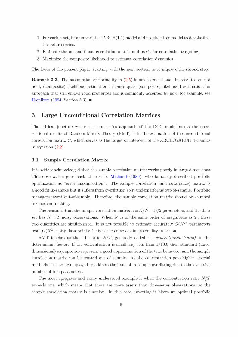
1. For each asset, fit a univariate GARCH(1,1) model and use the fitted model to devolatilize
the return series.
2. Estimate the unconditional correlation matrix and use it for correlation targeting.
3. Maximize the composite likelihood to estimate correlation dynamics.
The focus of the present paper, starting with the next section, is to improve the second step.
Remark 2.3. The assumption of normality in (2.5) is not a crucial one. In case it does not
hold, (composite) likelihood estimation becomes quasi (composite) likelihood estimation, an
approach that still enjoys good properties and is commonly accepted by now; for example, see
Hamilton (1994, Section 5.3).
3 Large Unconditional Correlation Matrices
The critical juncture where the time-series approach of the DCC model meets the cross-
sectional results of Random Matrix Theory (RMT) is in the estimation of the unconditional
correlation matrix C, which serves as the target or intercept of the ARCH/GARCH dynamics
in equation (2.2).
3.1 Sample Correlation Matrix
It is widely acknowledged that the sample correlation matrix works poorly in large dimensions.
This observation goes back at least to Michaud (1989), who famously described portfolio
optimization as “error maximization”. The sample correlation (and covariance) matrix is
a good fit in-sample but it suffers from overfitting, so it underperforms out-of-sample. Portfolio
managers invest out-of-sample. Therefore, the sample correlation matrix should be shunned
for decision making.
The reason is that the sample correlation matrix has N(N −1)/2 parameters, and the data
set has N × T noisy observations. When N is of the same order of magnitude as T , these
two quantities are similar-sized. It is not possible to estimate accurately O(N2) parameters
from O(N2) noisy data points: This is the curse of dimensionality in action.
RMT teaches us that the ratio N/T , generally called the concentration (ratio), is the
determinant factor. If the concentration is small, say less than 1/100, then standard (fixed-
dimensional) asymptotics represent a good approximation of the true behavior, and the sample
correlation matrix can be trusted out of sample. As the concentration gets higher, special
methods need to be employed to address the issue of in-sample overfitting due to the excessive
number of free parameters.
The most egregious and easily understood example is when the concentration ratio N/T
exceeds one, which means that there are more assets than time-series observations, so the
sample correlation matrix is singular. In this case, inverting it blows up optimal portfolio
5
weights to plus or minus infinity, which obviously is an economically incorrect solution. But
by continuity, as N gets closer to T , problems start to creep in. Indeed, the main lesson of
RMT is that, unless N/T is negligible, the sample correlation (and covariance) matrix will
systematically misbehave out of sample.
3.2 Shrinkage Estimator
Fortunately, recent developments have provided effective solutions to this problem. It is now
possible to rectify the in-sample bias of the sample correlation (or covariance) matrix due to
overfitting. This rectification takes place at the level of the eigenvalues. The small sample
eigenvalues are too small and the large ones too large. So it is just a matter of pushing up the
small ones and pulling down the large ones. Since this transformation reduces the spread of
the cross-sectional distribution of eigenvalues, it is generally called shrinkage.
In this paper, we will focus on the nonlinear shrinkage formula of Ledoit and Wolf (2012).
The intuition is as follows. Let Σ denote the population covariance matrix, S the sample
covariance matrix, and u an eigenvector of S. Then by basic linear algebra, the corresponding
sample eigenvalue is equal to u′Su. It is the in-sample variance of a portfolio with weights given
by the vector u. This is the quantity that needs to be rectified due to overfitting. Nonlinear
shrinkage replaces it with (a consistent estimator of) u′Σu, the out-of-sample variance of the
same portfolio. Clearly, we want to decide our portfolio allocation in the direction of the
vector u based on its true out-of-sample risk u′Σu, rather than its in-sample counterpart u′Su,
which is heavily biased due to the curse of dimensionality.
This may seem like magic: given that we do not know Σ, how could we know u′Σu?
However, Ledoit and Peche (2011) show that we do not need to know all of the true covariance
matrix Σ — which would be a hopeless task — but only its eigenvalues. There are just N of
them. Given a data set of dimension N × T , it is clearly impossible to estimate accurately a
whole matrix of dimension N ×N , but it is theoretically possible to estimate its N eigenvalues.
The ratio of parameters to data entries is 1/T , which is a small number, regardless of how big
the matrix dimension N is.
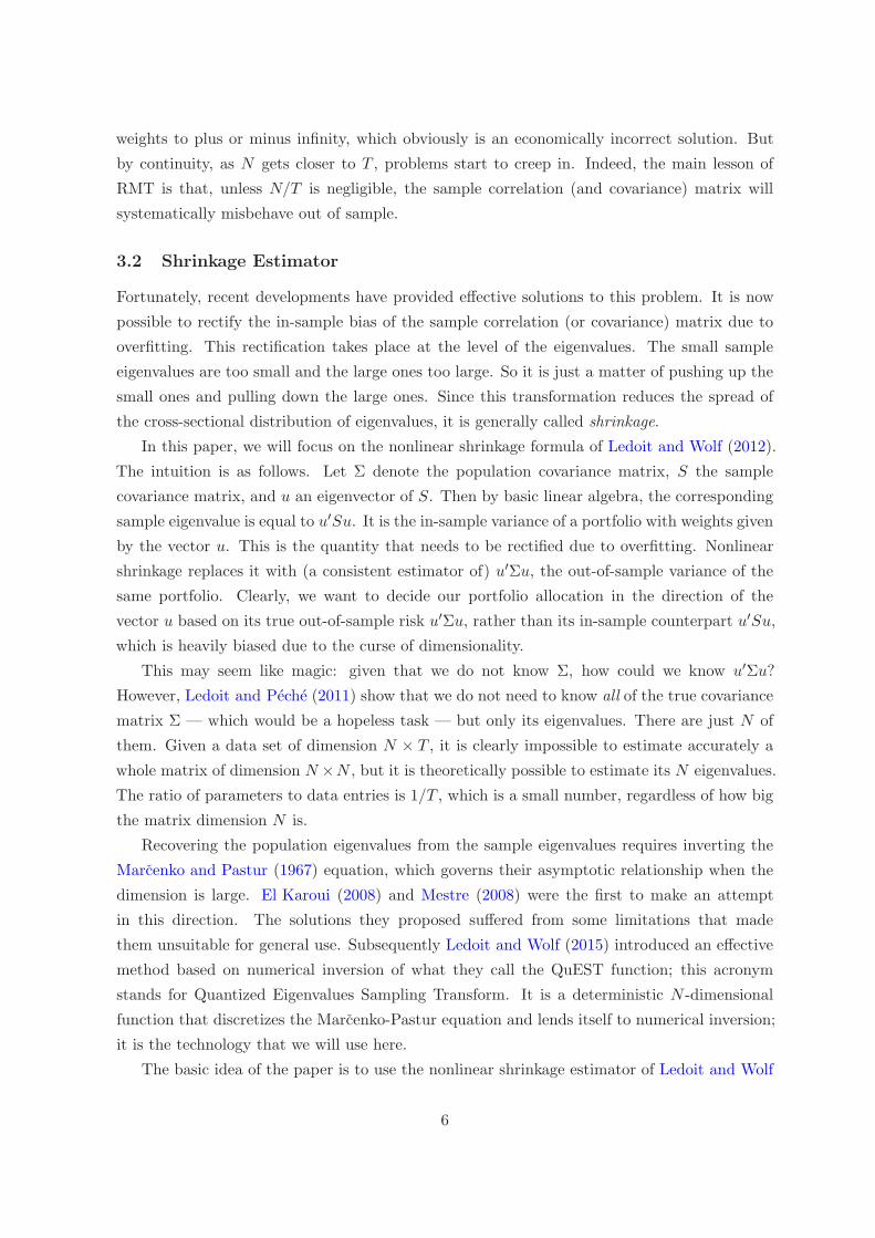
Recovering the population eigenvalues from the sample eigenvalues requires inverting the
Marcenko and Pastur (1967) equation, which governs their asymptotic relationship when the
dimension is large. El Karoui (2008) and Mestre (2008) were the first to make an attempt
in this direction. The solutions they proposed suffered from some limitations that made
them unsuitable for general use. Subsequently Ledoit and Wolf (2015) introduced an effective
method based on numerical inversion of what they call the QuEST function; this acronym
stands for Quantized Eigenvalues Sampling Transform. It is a deterministic N -dimensional
function that discretizes the Marcenko-Pastur equation and lends itself to numerical inversion;
it is the technology that we will use here.
The basic idea of the paper is to use the nonlinear shrinkage estimator of Ledoit and Wolf
6

(2012) to estimate the correlation targeting matrix C in equation (2.2) instead of the sample
correlation matrix. When the dimension N is large and of the same order of magnitude as the
sample size T , this approach generates an estimator of the conditional covariance matrix Ht
that has better out-of-sample properties.
3.3 Mathematical Formulation
Let S ..= [si,t] denote the N × T matrix of devolatilized returns. Assuming mean zero, its
sample covariance matrix is
C ..=1
TSS′. (3.1)
Decompose C it into a set of eigenvalues (λ1, λ2 . . . , λN ), sorted in descending order without
loss of generality, and corresponding eigenvectors (u1, u2, . . . , uN ); consequently
C =N∑
i=1
λiuiu′i. (3.2)
Let QN,T denote the QuEST function defined in Section 2.2 of Ledoit and Wolf (2015). It is
a multivariate deterministic function that maps [0,∞)N onto itself. Given a set of population
eigenvalues t ..= (t1, . . . , tN ) as input, it returns as output a deterministic equivalent of the
sample eigenvalues QN,T (t) =(q1N,T (t), q
2N,T (t), . . . , q
NN,T (t)
). Thus, population eigenvalues
can be estimated by numerically inverting the QuEST function:
τ ..= argmint∈[0,∞)N
1
N
N∑
i=1
[qiN,T (t)− λi
]2. (3.3)
Given estimated population eigenvalues τ = (τ1, τ2, . . . , τN ), we can then use Theorem 4 of
Ledoit and Peche (2011) to compute a nonlinear shrinkage formula that is asymptotically
optimal under large-dimensional asymptotics. Denote the shrunk eigenvalues by λ(τ ) ..=(λ1(τ ), λ2(τ ), . . . , λN (τ )
).
The mathematical expressions for the QuEST function and the nonlinear shrinkage formula
are quite involved, as they depend on the Stieltjes transform, an integral transform defined on
the upper half of the complex plane, so they will not be repeated here. The way to intuitively
understand λi(τ ) is that it is a consistent estimator for the out-of-sample variance u′iΣui under
large-dimensional asymptotics. The shrinkage estimator of the covariance matrix can then be
reconstructed as
C ..=N∑
i=1
λi(τ )uiu′i . (3.4)
Two important advantages of this approach are (i) that it does not require the assumption of
normality and (ii) that it can handle the challenging case where the number of assets exceeds
the sample size.
7

Supplementary Material 9 contains a primer on this technology imported from Probability
Theory and from Multivariate Statistics; see Ledoit and Wolf (2017a) for a more rigorous
exposition. In terms of assumptions on the data-generating process, Ledoit and Wolf (2017a)
do not assume normality, but assume that the 12th moment is finite. While this assumption
simplies the mathematical proofs, numerical simulations indicate that a bounded fourth
moment would be sufficient in practice.
3.4 Linear Shrinkage
A simpler alternative is to use the linear shrinkage formula of Ledoit and Wolf (2004b). Define
the cross-sectional average of sample eigenvalues as
λ ..=1
N
N∑
i=1
λi . (3.5)
This method provides a consistent estimator ρ for the optimal shrinkage intensity, which is
a number between zero and one controlling the amount by which the sample eigenvalues are
dragged towards their cross-sectional average λ. The linear shrinkage estimator is expressed as
C ..=N∑
i=1
[ρλ+ (1− ρ)λi
]uiu
′i . (3.6)
This estimator has proven quite popular with applied researchers but it is optimal only in
a class of dimension two, which is nested inside the class of dimension N over which nonlinear
shrinkage is optimal. Therefore, asymptotically, when N and T grow large together, nonlinear
shrinkage should perform better in the generic case. The main difference is that the shrinkage
intensity ρ is constrained to be the same for all eigenvalues under linear shrinkage, whereas it
is individually fitted to each eigenvalue under nonlinear shrinkage. This approach is obviously
more complicated but due to the highly nonlinear nature of the problem, it is also more powerful.
Hafner and Reznikova (2012) propose the application of linear shrinkage to the estimation of
DCC models. However, they restrict themselves to smaller dimensions and throw shrinkage
into a horse race against composite likelihood, instead of harnessing the combined powers of
the two methods. In addition, there is theoretical justification for upgrading from linear to
nonlinear shrinkage (Ledoit and Wolf, 2012).
Remark 3.1. As suggested by a referee, one can alternatively consider the linear shrinkage
method of Ledoit and Wolf (2004a) for the estimation of the intercept matrix C. This estimator
does not belong to the class of rotation-equivariant estimators studied by Ledoit and Wolf
(2012, 2015) and also described in Supplementary Material 9 for completeness.
3.5 Renormalization
In practice, the diagonal elements of C, C, and C tend to deviate from one slightly, in spite
of the fact that devolatilized returns are used as inputs. Therefore every column and every
8

row has to be divided by the square root of the corresponding diagonal entry, so as to produce
a proper correlation matrix.
4 Loss Function
This section builds upon Engle and Colacito (2006), hereafter abbreviated by EC. It is couched
in terms of the unconditional covariance matrix initially, and the adaptation to conditional
covariance matrices is described in Section 4.4. To make the exposition more fluid, the word
“return” stands for the raw return on a risky asset minus the risk-free interest rate.
4.1 Out-of-Sample Portfolio Variance
Let Σ denote the N -dimensional covariance matrix of returns, Σ a generic estimator of Σ,
and m an assumed vector of expected returns. EC’s equation (3) gives the out-of-sample
variance of the optimal portfolio based on the estimator Σ as
LV (Σ,Σ,m) ..=m′Σ−1ΣΣ−1m(m′Σ−1m
)2 . (4.1)
This loss function corresponds to the quintessential risk or error minimization objective. It
was also adopted by Ledoit and Wolf (2017a, Definition 2.1), up to rescaling by the squared
Euclidian norm of m. In addition, it captures the performance of a covariance matrix
estimator for mathematically equivalent problems where variance minimization decisions must
be taken, such as Capon (1969) beamforming in signal processing and optimal fingerprinting
in climatology (IPCC, 2007).
EC’s Theorem 1 demonstrates that LV is minimized when Σ = Σ, so if we want a loss
function that is always nonnegative, and is equal to zero when the covariance matrix estimator
happens to be equal to the truth — as is customary —, then we can compute the excess
portfolio variance caused by covariance matrix estimation error:
LE(Σ,Σ,m) ..= LV (Σ,Σ,m)− LV (Σ,Σ,m) =m′Σ−1ΣΣ−1m(m′Σ−1m
)2 − 1
m′Σ−1m≥ 0 . (4.2)
4.2 Expected Returns
The vector of expected returns that we have assumed is not required to be equal to the true one.
Different investors will have different models of expected returns. This suggests investigating
over a wide range of alternatives form. The idea is to integrate the excess portfolio variance LE
over a relevant manifold of expected return vectors.
The relative efficiency of two covariance matrix estimators is unaffected by the norm of the
vector m, so we can take ‖m‖ = 1 without loss of generality, where ‖ · ‖ denotes the Euclidian
9

norm. For this reason, in dimension 2, EC’s Section 2.1 considers expected returns of the form
m = [cos(θ), sin(θ)]′ where θ is some angle. The generalization in dimension N is to consider
vectors m that belong to the N -dimensional unit sphere UN..= {x ∈ R
N : ‖x‖ = 1}. Averagingout the excess portfolio variance across all possible m’s in this manifold leads to a loss function
that depends solely on covariance matrices:
LI(Σ,Σ) ..=
∫
UN
LE(Σ,Σ, µ) dµ =
∫
UN
[µ′Σ−1ΣΣ−1µ(µ′Σ−1µ
)2 − 1
µ′Σ−1µ
]dµ , (4.3)
where∫UN
denotes the integral over the N -dimensional unit sphere. The intuition is that we
want a covariance matrix estimator that is the best ‘all-rounder’ and thus performs well across
the board. Given that this paper focuses explicitly on the second moments, we are not in
a position to take a stance on the orientation of the linear constraint vector.
4.3 Equivalent Formulation Under Large-Dimensional Asymptotics
The integral in LI is not easy to evaluate analytically. At this juncture, we can get help from
a foundational lemma in Random Matrix Theory (RMT):
x′Ax ≈ Tr(A) ‖x‖2N
, (4.4)
where Tr(·) denotes the trace of a matrix, A is some symmetric random matrix of large
dimension N , and x is an N -dimensional vector not statistically related to A, that is, x is
distributed independently of A and its distribution is rotation-invariant. Rigorous versions of
equation (4.4) appear decisively as Lemma 1 of Marcenko and Pastur (1967), Lemma 3.1 of
Silverstein and Bai (1995), and Lemma 1 of Ledoit and Peche (2011). This is basically a cross-
sectional law of large numbers. Indeed if, conditional on A, x follows the standard multivariate
normal distribution, then even in finite samples the relation
E
[x′Ax
∣∣∣∣A]= E
[Tr(A) ‖x‖2
N
∣∣∣∣A]
(4.5)
holds exactly. Injecting (4.4) into the loss function LI naturally suggests the alternative loss
function L, which is significantly easier to evaluate.
Definition 4.1. The loss function is defined as
L(Σ,Σ
).
.=Tr(Σ−1ΣΣ−1
)/N
[Tr(Σ−1
)/N]2 − 1
Tr(Σ−1
)/N
. (4.6)
This is the loss function that will be used throughout the rest of the paper. The formulations
LI and L are interchangeable under large-dimensional asymptotics, as the following proposition
attests.
10

Proposition 4.1. Under the assumptions of Theorem 3.1 of Ledoit and Wolf (2017a), both
loss functions LI
(Σ,Σ
)and L
(Σ,Σ
)converge almost surely to the same, non-stochastic limit
as T → ∞ with N/T → c ∈ (0, 1).
Proof. Let m be a random vector distributed according to the N -dimensional standard
multivariate normal distribution, independently from Σ. Thenm/‖m‖ is uniformly distributed
on UN . This implies that
LI(Σ,Σ) = E[LE
(Σ,Σ,m/‖m‖
)∣∣∣ Σ]. (4.7)
Proposition 4.1 then follows directly by injecting Lemma 1 of Ledoit and Peche (2011) into
the proof of Theorem 3.1 of Ledoit and Wolf (2017a).
A traditional property of a loss function is that if one plugs the population parameters into
the loss function, the value of the loss is zero. By convention, there is no loss from estimation if
somehow you happen to know the truth; the loss should only be strictly positive if the estimator
has error in it. The following theorem, which is equivalent in spirit to EC’s Theorem 1, shows
that the loss function in Definition 4.1 possesses the desired property.
Theorem 4.1. L(Σ,Σ
)≥ 0; and L
(Σ,Σ
)= 0 ⇐⇒ ∃ γ > 0 s.t. Σ = γΣ.
Proof. It is a standard result in linear algebra that, for any two symmetric positive-definite
matrices Σ and Σ, there exists an invertible matrix A such that
A′ΣA = IN (4.8)
A′ΣA = ∆ , (4.9)
where the superscript ′ denotes the transpose of a matrix, IN denotes the identity matrix of
dimension N , and ∆ denotes some diagonal matrix with strictly positive diagonal elements.
Substituting equations (4.8)–(4.9) into the definition (4.6) yields
L(Σ,Σ
)≥ 0 ⇐⇒ Tr
(∆−2A′A
)× Tr
(A′A
)≥[Tr(∆−1A′A
)]2. (4.10)
Denote the ith diagonal element of ∆ by δi and the ith diagonal element of A′A by αi,
for i = 1, . . . , N . Note that ∀i = 1, . . . , N , αi > 0 and δi > 0. Then,
L(Σ,Σ
)≥ 0 ⇐⇒
(N∑
i=1
αi
δ2i
)(N∑
i=1
αi
)≥(
N∑
i=1
αi
δi
)2
. (4.11)
Define xi ..=√αi/δi and yi ..=
√αi, for i = 1, . . . , N . Then
L(Σ,Σ
)≥ 0 ⇐⇒
(N∑
i=1
x2i
)(N∑
i=1
y2i
)≥(
N∑
i=1
xiyi
)2
. (4.12)
11

On the right-hand side of the equivalency we recognize the Cauchy-Schwarz inequality;
therefore, the loss function is always non-negative. For equality to hold, we need the vectors
(x1, . . . , xN )′ and (y1, . . . , yN )′ to be collinear, which implies that the diagonal matrix ∆ is
a scalar multiple of the identity. Inspecting equations (4.8)–(4.9) reveals that this can only
happen if the estimator Σ is a scalar multiple of the true covariance matrix Σ.
4.4 Adaptation for Conditional Covariance Matrices
Given that the loss function from Definition 4.1 is suitable for unconditional covariance
matrices, it must be adapted for conditional ones. Let Ht denote a generic estimator of the
true conditional covariance matrix Ht (for t = 1, . . . , T ). Then the average loss is given by
L ..=1
T
T∑
i=1
L(Ht, Ht
). (4.13)
This is the quantity that will be reported in all Monte Carlo simulations below.
5 Monte Carlo Simulations
5.1 Base-Case Scenario
In order to carry out realistic Monte Carlo simulations, we estimate the unconditional
population covariance matrix from the N ∈ {100, 500, 1000} most liquid stocks in the CRSP
database using ten years of daily data from 2005 through 2014. This matrix will be taken as
the ‘true’ unconditional covariance matrix in all the simulations.
We then simulate a DCC model with parameters α = 0.05 and β = 0.93 as in Pakel et al.
(2014, Table 4). According to (2.5), the DCC variates are drawn a from a multivariate standard
normal distribution, that is,
rt = H1/2t zt with zt
iid∼ N(0, IN ) . (5.1)
The univariate volatility dynamics are governed by GARCH(1,1) models with identical
parameters ai = 0.05 and bi = 0.90 across all stocks i = 1, . . . , N .
For each simulation, we generate an N × T matrix of simulated returns, where the sample
size is T = 1250. This sample size corresponds to approximately five years of daily data, an
estimation window commonly used in practice. Thus, the concentration ratio for the broadest
universe is c ..= N/T = 0.8, which is not negligible, and we can expect substantial shrinkage
effects. Even though we could potentially accommodate the case c > 1, we choose a value
of c less than one so that the sample correlation matrix can be used as a benchmark. In any
case, having a universe of 1000 assets in which to invest is sufficiently broad for most portfolio
managers.
12

5.2 Numerical Details
The nonlinear shrinkage estimator of the correlation targeting matrix is computed in Matlab
using version 025 of the QuEST package. It contains the QuEST function itself, a routine
to invert it numerically by using a nonlinear optimizer, and another routine to compute the
optimal nonlinear shrinkage formula. The end user does not have to do anything except
input the raw data and collect the shrinkage estimator. The linear shrinkage estimator of
the correlation targeting matrix is also computed in Matlab using codes that implement the
formulas of Ledoit and Wolf (2004a,b). All codes are available from the university faculty
website of Michael Wolf.
The program to simulate the DCC model has been adapted from Kevin Sheppard’s legacy
UCSD GARCH Toolbox. The program to estimate the DCC model has been based on the
successor to the UCSD GARCH Toolbox, which is the Oxford MFE Toolbox, also by Kevin
Sheppard.
We have made two important modifications to the latter. The first one was to add the
flexibility to shrink the eigenvalues of the sample correlation matrix used for correlation
targeting as delineated in Section 3. The second one was to rewrite the function that computes
the composite likelihood in a way that is improved in terms of speed and memory management;
this rewriting required, among other things, translating the Matlab code into the C language,
which in this case can generate substantial speed advantage, if used judiciously. The end result
is that we can go to N = 1000 assets without running out of memory, and it takes less than
three minutes to estimate the DCC model with nonlinear shrinkage, a speed gain by a factor
of at least 20. (These numbers correspond to using Matlab R2016a on an Apple Mac Pro with
a 3.5 GHz Intel Xeon E5 processor and 60GB of memory.)
5.3 List of Candidate Estimators
It is clearly beyond the scope of the present paper to compare all the covariance matrix
estimators in the literature. Therefore, we focus on the following representative set of six
candidates:
• DCC-S: DCC with the correlation targeting matrix C estimated by the sample
covariance matrix of devolatilized returns.
• DCC-L1: DCC with C estimated by the linear shrinkage estimator of Ledoit and Wolf
(2004b), whose shrinkage target is (a multiple of) the identity matrix.
• DCC-L2: DCC with C estimated by the linear shrinkage estimator of Ledoit and Wolf
(2004a), whose shrinkage target is the constant-correlation matrix.
• DCC-NL: DCC with C estimated by the nonlinear shrinkage estimator; this is the main
focus of our paper.
13

• CCC-NL: The Constant Conditional Correlation model using Qt ≡ C, with C estimated
by non-linear shrinkage as in DCC-NL.
• RM-2006: The RiskMetrics 2006 methodology detailed by Zumbach (2007) and
implemented in Kevin Sheppard’s Matlab routine riskmetrics2006.
5.4 Results
The results averaged across 105/N Monte Carlo simulations are presented in Table 1. (Note
that in large dimensions, such as N = 1000, the results are extremely consistent from one
simulation to the next, so there is no need to go to thousands of simulations.)
N DCC-S DCC-L1 DCC-L2 DCC-NL CCC-NL RM-2006
100 0.061 0.060 0.054 0.055 0.103 0.086
500 0.120 0.098 0.070 0.066 0.092 0.194
1000 0.421 0.147 0.087 0.079 0.099 0.602
Table 1: Average loss for six different covariance matrix estimators in dimensions
N ∈ {100, 500, 1000} with sample size T = 1250. The unit is 10−3. The lowest
number in each row appears in bold face.
DCC-NL dominates across the board in large dimensions, but for N = 100 linear shrinkage
towards the constant-correlation matrix does slightly better. This is probably due to the fact
that we calibrated our population unconditional correlation matrix to actual stock returns
data, for which constant correlation happens to be a parsimonious yet accurate model. As the
cross-section increases, DCC-NL has more information to pick up on, which enables it to first
beat DCC-L2 and to then widen the gap.
An intuitive way to quantify the improvement is to compute the Percentage Relative
Improvement in Average Loss (PRIAL). For example, the PRIAL of DCC-NL with respect
to DCC-S is defined as
100×
1−
E[LDCC-NL
]
E[LDCC-S
]
% , (5.2)
where the loss L for each estimator is calculated as per equation (4.13) and the expectation is
taken across Monte Carlo simulations. By construction, the PRIAL (5.2) of the true conditional
covariance matrix with respect to DCC-S is 100%, which is the maximum attainable; on the
other hand, 0% means no improvement at all.
The interpretation is that, as long as we do not know the true conditional covariance matrix,
estimation error will cause excess out-of-sample portfolio variance, and we want to eliminate
as much of it as possible. The PRIAL of DCC-NL with respect to a given estimator (such as
14
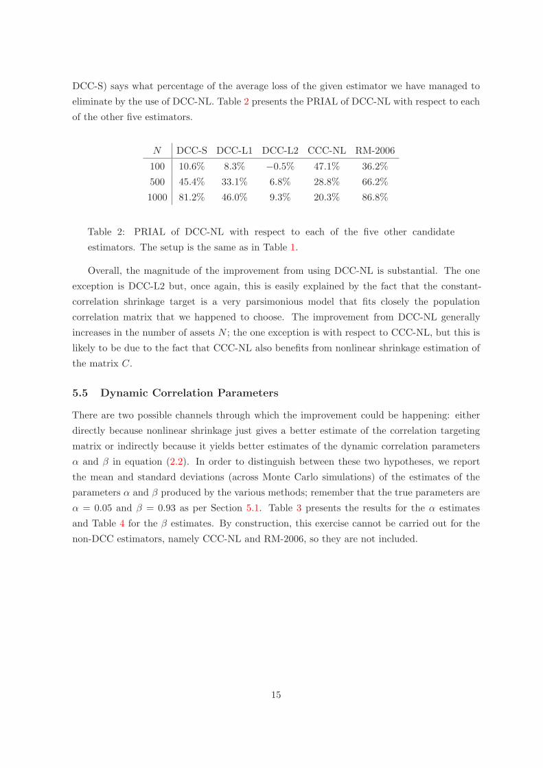
DCC-S) says what percentage of the average loss of the given estimator we have managed to
eliminate by the use of DCC-NL. Table 2 presents the PRIAL of DCC-NL with respect to each
of the other five estimators.
N DCC-S DCC-L1 DCC-L2 CCC-NL RM-2006
100 10.6% 8.3% −0.5% 47.1% 36.2%
500 45.4% 33.1% 6.8% 28.8% 66.2%
1000 81.2% 46.0% 9.3% 20.3% 86.8%
Table 2: PRIAL of DCC-NL with respect to each of the five other candidate
estimators. The setup is the same as in Table 1.
Overall, the magnitude of the improvement from using DCC-NL is substantial. The one
exception is DCC-L2 but, once again, this is easily explained by the fact that the constant-
correlation shrinkage target is a very parsimonious model that fits closely the population
correlation matrix that we happened to choose. The improvement from DCC-NL generally
increases in the number of assets N ; the one exception is with respect to CCC-NL, but this is
likely to be due to the fact that CCC-NL also benefits from nonlinear shrinkage estimation of
the matrix C.
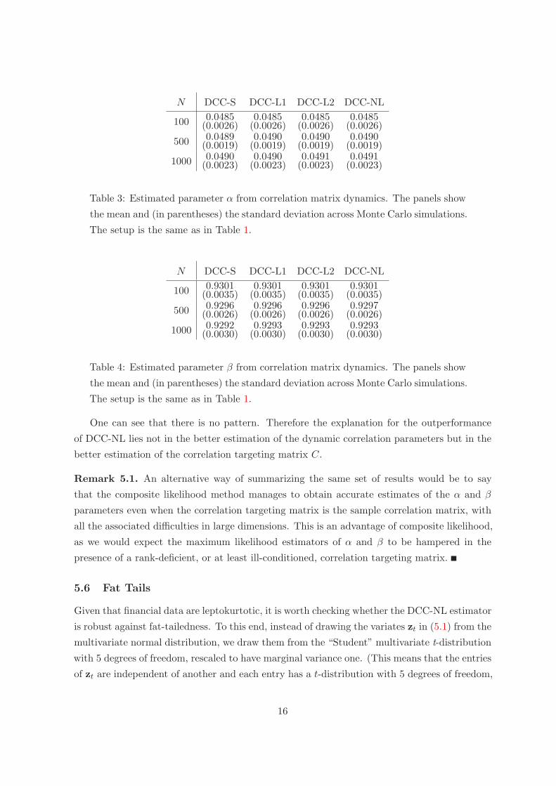
5.5 Dynamic Correlation Parameters
There are two possible channels through which the improvement could be happening: either
directly because nonlinear shrinkage just gives a better estimate of the correlation targeting
matrix or indirectly because it yields better estimates of the dynamic correlation parameters
α and β in equation (2.2). In order to distinguish between these two hypotheses, we report
the mean and standard deviations (across Monte Carlo simulations) of the estimates of the
parameters α and β produced by the various methods; remember that the true parameters are
α = 0.05 and β = 0.93 as per Section 5.1. Table 3 presents the results for the α estimates
and Table 4 for the β estimates. By construction, this exercise cannot be carried out for the
non-DCC estimators, namely CCC-NL and RM-2006, so they are not included.
15
N DCC-S DCC-L1 DCC-L2 DCC-NL
100 0.0485(0.0026)
0.0485(0.0026)
0.0485(0.0026)
0.0485(0.0026)
500 0.0489(0.0019)
0.0490(0.0019)
0.0490(0.0019)
0.0490(0.0019)
1000 0.0490(0.0023)
0.0490(0.0023)
0.0491(0.0023)
0.0491(0.0023)
Table 3: Estimated parameter α from correlation matrix dynamics. The panels show
the mean and (in parentheses) the standard deviation across Monte Carlo simulations.
The setup is the same as in Table 1.
N DCC-S DCC-L1 DCC-L2 DCC-NL
100 0.9301(0.0035)
0.9301(0.0035)
0.9301(0.0035)
0.9301(0.0035)
500 0.9296(0.0026)
0.9296(0.0026)
0.9296(0.0026)
0.9297(0.0026)
1000 0.9292(0.0030)
0.9293(0.0030)
0.9293(0.0030)
0.9293(0.0030)
Table 4: Estimated parameter β from correlation matrix dynamics. The panels show
the mean and (in parentheses) the standard deviation across Monte Carlo simulations.
The setup is the same as in Table 1.
One can see that there is no pattern. Therefore the explanation for the outperformance
of DCC-NL lies not in the better estimation of the dynamic correlation parameters but in the
better estimation of the correlation targeting matrix C.
Remark 5.1. An alternative way of summarizing the same set of results would be to say
that the composite likelihood method manages to obtain accurate estimates of the α and β
parameters even when the correlation targeting matrix is the sample correlation matrix, with
all the associated difficulties in large dimensions. This is an advantage of composite likelihood,
as we would expect the maximum likelihood estimators of α and β to be hampered in the
presence of a rank-deficient, or at least ill-conditioned, correlation targeting matrix.
5.6 Fat Tails
Given that financial data are leptokurtotic, it is worth checking whether the DCC-NL estimator
is robust against fat-tailedness. To this end, instead of drawing the variates zt in (5.1) from the
multivariate normal distribution, we draw them from the “Student” multivariate t-distribution
with 5 degrees of freedom, rescaled to have marginal variance one. (This means that the entries
of zt are independent of another and each entry has a t-distribution with 5 degrees of freedom,
16

rescaled to have variance one.) All other configurations are as per the base-case scenario
presented in Section 5.1. The results are presented in Table 5.
N DCC-S DCC-L1 DCC-L2 CCC-NL RM-2006
100 10.0% 7.8% −0.2% 44.4% 34.2%
500 44.5% 32.6% 6.9% 28.2% 65.4%
1000 80.8% 45.6% 9.3% 19.5% 86.5%
Table 5: PRIAL of DCC-NL with respect to each of the five other candidate
estimators. DCC variates are generated according to the “Student” t-distribution
with 5 degrees of freedom, rescaled to have marginal variance one.
Overall, the changes with respect to Table 2 are minimal, and there is no discernible pattern.
Therefore the conclusions reached in Section 5.4 are confirmed.
5.7 Misspecified Model
Although we know that multivariate GARCH effects are prevalent in financial data, it is
possible that the ‘true’ data generating process differs from the DCC model. In such a case, it
would be helpful to know that DCC-NL can still add value by producing conditional covariance
matrix estimators that are robust against model misspecification and continue to be relatively
accurate.
To this end, we simulate data from the BEKK model presented in Engle and Kroner (1995).
In practice, we take the Matlab function scalar vt vech simulate from Kevin Sheppard’s
Oxford MFE Toolbox. All the other configurations are as per the base-case scenario. The
results are presented in Table 6.
N DCC-S DCC-L1 DCC-L2 CCC-NL RM-2006
100 20.3% 17.8% 5.1% 72.5% 72.1%
500 54.3% 47.1% 19.3% 41.0% 79.7%
1000 85.4% 65.2% 24.1% 26.8% 91.3%
Table 6: PRIAL of DCC-NL with respect to each of the five other candidate
estimators. Data are generated from the BEKK model.
Compared with Table 2, the PRIAL of DCC-NL with respect to each of its five competitors
always goes up. The differences in PRIALs (that is, the entry in Table 6 minus the
corresponding entry in Table 2) range from a low of +4.5% to a high of +35.9%, with an
average additive boost of +13.1%. Thus, an additional advantage of DCC-NL is that it appears
more robust against model misspecification than other comparable estimators.
17

6 Empirical Results
The goal of this section is to examine the out-of-sample properties of Markowitz portfolios based
on our newly suggested covariance matrix estimator. There are a myriad of popular investment
strategies by now and it is not our goal to compare to an extensive list of them. The only focus
of this section is compare nonlinear DCC to a selection of seven other representative portfolio
selection strategies.
For compactness of notation, we do not use the subscript T in denoting the covariance
matrix itself, an estimator of the covariance matrix, or a return-predictive signal that proxies
for the vector of expected returns.
6.1 Data and General Portfolio-Formation Rules
We download daily data from the Center for Research in Security Prices (CRSP) starting
in 01/01/1980 and ending in 12/31/2015. For simplicity, we adopt the common convention
that 21 consecutive trading days constitute one ‘month’. The out-of-sample period ranges
from 01/08/1986 through 12/31/2015, resulting in a total of 360 ‘months’ (or 7560 days).
All portfolios are updated ‘monthly’. (‘Monthly’ updating is common practice to avoid an
unreasonable amount of turnover and thus transaction costs. During a ‘month’, from one day
to the next, we hold number of shares fixed rather than portfolio weights; in this way, there
are no transactions at all during a ‘month’.)
We denote the investment dates by h = 1, . . . , 360. At any investment date h, a covariance
matrix is estimated using the most recent T = 1250 daily returns, which roughly corresponds
to using five years of past data.
We consider the following portfolio sizes: N ∈ {100, 500, 1000}. For a given combination
(h,N), the investment universe is obtained as follows. We find the set of stocks that have
a complete return history over the most recent T = 1250 days as well as a complete return
‘future’ over the next 21 days. (The latter, forward-looking restriction is not a feasible one
in real life but is commonly applied in the related finance literature on the out-of-sample
evaluation of portfolios.) We then look for possible pairs of highly correlated stocks, that is,
pairs of stocks that returns with a sample correlation exceeding 0.95 over the past 1250 days.
With such pairs, if they should exist, we remove the stock with the lower volume of the two on
investment date h. (The reason is that we do not want to include highly similar stocks; in the
early years, there are no such pairs; in the most recent years, there are never more than three
such pairs.) Of the remaining set of stocks, we then pick the largest N stocks (as measured by
their market capitalization on investment date h) as our investment universe. In this way, the
investment universe changes slowly from one investment date to the next.
18

6.2 Global Minimum Variance Portfolio
We consider the problem of estimating the global minimum variance (GMV) portfolio, in the
absence of short-sales constraints. The problem is formulated as
minww′Htw (6.1)
subject to w′1 = 1 , (6.2)
where 1 denotes a vector of ones of dimension N × 1. It has the analytical solution
w =H−1
t 1
1′H−1t 1
. (6.3)
The natural strategy in practice is to replace the unknown Ht by an estimator Ht in
formula (6.3), yielding a feasible portfolio
w ..=H−1
t 1
1′H−1t 1
. (6.4)
Estimating the GMV portfolio is a ‘clean’ problem in terms of evaluating the quality of a
covariance matrix estimator, since it abstracts from having to estimate the vector of expected
returns at the same time. In addition, researchers have established that estimated GMV
portfolios have desirable out-of-sample properties not only in terms of risk but also in terms of
reward-to-risk , that is, in terms of the information ratio; for example, see Haugen and Baker
(1991), Jagannathan and Ma (2003), and Nielsen and Aylursubramanian (2008). As a result,
such portfolios have become an addition to the large array of products sold by the mutual-fund
industry.
The following eight portfolios are included in the study.
• 1/N : the equal-weighted portfolio. This portfolio is a standard benchmark and has been
promoted by DeMiguel et al. (2009), among others.
• DCC-S: the portfolio (6.4), where the estimator Ht is obtained from DCC based on the
sample correlation matrix.
• DCC-L1: the portfolio (6.4), where the estimator Ht is obtained from DCC based on
the linear shrinkage of Ledoit and Wolf (2004b).
• DCC-L2: the portfolio (6.4), where the estimator Ht is obtained from DCC based on
the linear shrinkage of Ledoit and Wolf (2004a).
• DCC-NL: the portfolio (6.4), where the estimator Ht is obtained from DCC based on
nonlinear shrinkage.
• NL-DCC: the portfolio (6.4), where the estimator Ht is obtained by post-processing the
DCC-S estimator of Ht with nonlinear shrinkage.
19

• CCC-NL: the portfolio (6.4), where the estimator Ht is obtained from CCC based on
nonlinear shrinkage. This means that instead of the DCC dynamics of model (2.2),
one considers the static constant-conditional-correlation model Qt ≡ C; in practice, the
estimator of C is obtained by nonlinear shrinkage just as in DCC-NL.
• RM-2006: the portfolio (6.4), where the estimator Ht is obtained from the RiskMetrics
2006 methodology; see Zumbach (2007). (We use the Matlab routine riskmetrics2006
provided by Kevin Sheppard.)
We report the following three out-of-sample performance measures for each scenario. (All
of them are annualized and in percent for ease of interpretation.)
• AV: We compute the average of the 7560 out-of-sample log returns and then multiply
by 252 to annualize.
• SD: We compute the standard deviation of the 7560 out-of-sample log returns and then
multiply by√252 to annualize.
• IR: We compute the (annualized) information ratio as the ratio AV/SD.
Our stance is that in the context of the GMV portfolio, the most important performance
measure is the out-of-sample standard deviation, SD. The true (but unfeasible) GMV portfolio
is given by (6.3). It is designed to minimize the variance (and thus the standard deviation)
rather than to maximize the expected return or the information ratio. Therefore, any
portfolio that implements the GMV portfolio should be primarily evaluated by how successfully
it achieves this goal. A high out-of-sample average return, AV, and a high out-of-sample
information ratio, IR, are naturally also desirable, but should be considered of secondary
importance from the point of view of evaluating the quality of a covariance matrix estimator.
We also consider the question of whether DCC-NL delivers a lower out-of-sample standard
deviation than DCC-S at a level that is statistically significant. For a given universe size N ,
a two-sided p-value for the null hypothesis of equal standard deviations is obtained by the
prewhitened HACPW method described in Ledoit and Wolf (2011, Section 3.1).
The results are presented in Table 7 and can be summarized as follows; unless stated
otherwise, the findings are with respect to the out-of-sample standard deviation as performance
measure.
• All other portfolios consistently outperform 1/N by a wide margin. In addition, all DCC
and CCC portfolios also outperform RM-2006 by substantial margin.
• Among the DCC portfolios, there is a consistent ranking across all portfolio sizes N :
DCC-NL, NL-DCC, DCC-L2, DCC-L1, and DCC-S.
• The second-best portfolio consistently is CCC-NL, that is, its performance ranks between
DCC-NL and NL-DCC.
20

• The outperformance of DCC-NL over DCC-S is always statistically significant and it is
also economically meaningful for N = 500, 1000.
• DeMiguel et al. (2009) claim that it is difficult to outperform 1/N in terms of the out-
of-sample Sharpe ratio with ‘sophisticated’ portfolios (that is, with Markowitz portfolios
that estimate input parameters). It can be seen that all other portfolios consistently
outperform 1/N in terms of the out-of-sample information ratio, which translates into
outperformance in terms of the out-of-sample Sharpe ratio. For N = 100, CCC-NL is
best overall, whereas for N = 500, 1000, DCC-NL is best overall.
Period: 01/08/1986–12/31/2015
1/N DCC-S DCC-L1 DCC-L2 DCC-NL NL-DCC CCC-NL RM-2006
N = 100
AV 12.10 9.92 9.91 9.91 9.95 10.24 11.37 8.41
SD 21.56 13.36 13.33 13.27 13.17∗∗∗ 13.22 13.20 14.69
IR 0.56 0.74 0.74 0.74 0.76 0.77 0.86 0.57
N = 500
AV 13.46 13.94 13.88 13.76 13.38 10.87 13.25 11.26
SD 19.53 10.57 10.40 10.16 9.64∗∗∗ 9.93 9.74 12.60
IR 0.69 1.32 1.33 1.35 1.39 1.09 1.36 0.89
N = 1000
AV 14.21 11.77 12.15 11.88 12.17 11.12 11.72 11.37
SD 19.04 10.59 9.14 8.55 8.02∗∗∗ 8.79 8.13 14.86
IR 0.75 1.11 1.33 1.38 1.52 1.27 1.44 0.77
Table 7: Annualized performance measures (in percent) for various estimators of the GMV
portfolio. AV stands for average; SD stands for standard deviation; and IR stands for
information ratio. All measures are based on 7560 daily out-of-sample returns from 01/08/1986
through 12/31/2015. In the rows labeled SD, the lowest number appears in bold face. In the
columns labeled DCC-S and DCC-NL, significant outperformance of one of the two portfolios
over the other in terms of SD is denoted by asterisks: *** denotes significance at the 0.01 level;
** denotes significance at the 0.05 level; and * denotes significance at the 0.1 level.
6.3 Markowitz Portfolio with Momentum Signal
We now turn attention to a ‘full’ Markowitz portfolio with a signal.
By now a large number of variables have been documented that can be used to construct a
signal in practice. For simplicity and reproducibility, we use the well-known momentum factor
21
(or simply momentum for short) of Jegadeesh and Titman (1993). For a given investment
period h and a given stock, the momentum is the geometric average of the previous 252 returns
on the stock but excluding the most recent 21 returns; in other words, one uses the geometric
average over the previous ‘year’ but excluding the previous ‘month’. Collecting the individual
momentums of all the N stocks contained in the portfolio universe yields the return-predictive
signal m.
In the absence of short-sales constraints, the investment problem is formulated as
minww′Htw (6.5)
subject to w′m = b , and (6.6)
w′1 = 1 , (6.7)
where b is a selected target expected return. The problem has the analytical solution
w = c1H−1t 1+ c2H
−1t m , (6.8)
where c1 ..=C − bB
AC −B2and c2 ..=
bA−B
AC −B2, (6.9)
with A ..= 1′H−1t 1 , B ..= 1′H−1
t b , and C ..= m′H−1t m . (6.10)
The natural strategy in practice is to replace the unknown Ht by an estimator Ht in
formulas (6.8)–(6.10), yielding a feasible portfolio
w ..= c1H−1t 1+ c2H
−1t m , (6.11)
where c1 ..=C − bB
AC −B2and c2 ..=
bA−B
AC −B2, (6.12)
with A ..= 1′H−1t 1 , B ..= 1′H−1
t b , and C ..= m′H−1t m . (6.13)
The following eight portfolios are included in the study.
• EW-TQ The equal-weighted portfolio of the top-quintile stocks according to momen-
tum m. This strategy does not make use of the momentum signal beyond sorting of the
stocks in quintiles.
The value of the target expected return b for the remaining four portfolios below is then
given by the arithmetic average of the momentums of the stocks included in this portfolio
(that is, the expected return of EW-TQ according to the signal m).
• DCC-S: the portfolio (6.8)–(6.10), where the estimator Ht is obtained from DCC based
on the sample correlation matrix.
• DCC-L1: the portfolio (6.8)–(6.10), where the estimator Ht is obtained from DCC
based on the linear shrinkage of Ledoit and Wolf (2004a).
• DCC-L2: the portfolio (6.8)–(6.10), where the estimator Ht is obtained from DCC
based on the linear shrinkage of Ledoit and Wolf (2004a).
22

• DCC-NL: the portfolio (6.8)–(6.10), where the estimator Ht is obtained from DCC
based on nonlinear shrinkage.
• NL-DCC: the portfolio (6.8)–(6.10), where the estimator Ht is obtained by post-
processing the DCC-S estimator of Ht with nonlinear shrinkage.
• CCC-NL: the portfolio (6.8)–(6.10), where the estimator Ht is obtained from CCC based
on nonlinear shrinkage. This means that instead of the DCC dynamics of model (2.2),
one considers the static constant-conditional-correlation model Qt ≡ C; in practice, the
estimator of C is obtained by nonlinear shrinkage just as in DCC-NL. Note that CCC-NL
can be interpreted as a robustification of the CCC model of Bollerslev (1990) against large
dimensions.
• RM-2006: the portfolio (6.8)–(6.10), where the estimator Ht is obtained from the
RiskMetrics 2006 methodology; see Zumbach (2007). (We use the Matlab routine
riskmetrics2006 provided by Kevin Sheppard.)
Our stance is that in the context of a ‘full’ Markowitz portfolio, the most important
performance measure is the out-of-sample information ratio, IR. In the ‘ideal’ investment
problem (6.8)–(6.10), minimizing the variance (for a fixed target expected return b) is equivalent
to maximizing the information ratio (for a fixed target expected return b). In practice, because
of estimation error in the signal, the various strategies do not have the same expected return
and, thus, focusing on the out-of-sample standard deviation is inappropriate.
We also consider the question whether DCC-NL delivers a higher out-of-sample information
ratio than DCC-S at a level that is statistically significant. For a given universe size N , a two-
sided p-value for the null hypothesis of equal information ratios is obtained by the prewhitened
HACPW method described in Ledoit and Wolf (2008, Section 3.1).
The results are presented in Table 8 and can be summarized as follows; unless stated
otherwise, the findings are with respect to the out-of-sample information ratio as performance
measure.
• With the exception of RM-2006, all other portfolios consistently outperform EW-TQ by
a wide margin.
• Among the DCC portfolios, DCC-NL is consistently best followed by DCC-L2. NL-DCC
does well for N = 1000 but badly for N = 100, 500.
• The CCC-NL portfolio is second best for N = 500, 1000 but does badly for N = 100.
• The outperformance of DCC-NL over DCC-S is statistically significant and also
economically meaningful for N = 500, 1000.
• The performance of RM-2006 is disappointing. It is always worse than DCC-S and for
N = 1000 is also worse than EW-TQ.
• DeMiguel et al. (2009) claim that it is difficult to outperform 1/N in terms of the out-
of-sample Sharpe ratio with ‘sophisticated’ portfolios (that is, with Markowitz portfolios
23

that estimate input parameters). Comparing Table 8 with Table 7, it can be seen that
all DCC variants of the ‘full’ Markowitz portfolio consistently outperform 1/N in terms
of the out-of-sample information ratio, which translates into outperformance in terms of
the out-of-sample Sharpe ratio.
Even though momentum is not a very powerful return-predictive signal, the differences
can be enormous. For example, for N = 1000, the information ratio of 1/N is only 0.75
whereas the information ratio of DCC-NL is 1.62, more than twice as large.
• Engle and Colacito (2006) argue for the use of the out-of-sample standard deviation, SD,
as a performance measure also in the context of a ‘full’ Markowitz portfolio. Also for
this alternative performance measure, all DCC variants consistently outperform EW-TQ
by a wide margin. Furthermore, DCC-NL consistently has the smallest out-of-sample
standard deviation and its outperformance over DCC-S is always statistically significant.
Period: 01/08/1986–12/31/2015
EW-TQ DCC-S DCC-L1 DCC-L2 DCC-NL NL-DCC CCC-NL RM-2006
N = 100
AV 17.13 15.79 15.79 15.77 15.77 15.09 15.65 15.96
SD 28.43 17.05 17.03 16.99 16.90∗∗∗ 16.88 17.02 18.87
IR 0.60 0.93 0.93 0.93 0.93 0.89 0.92 0.85
N = 500
AV 17.15 16.60 16.66 16.55 16.78 14.53 16.13 16.50
SD 24.42 12.36 12.16 11.87 11.31∗∗∗ 11.87 11.55 16.14
IR 0.70 1.34 1.37 1.40 1.48∗∗ 1.22 1.40 1.02
N = 1000
AV 17.35 12.78 13.96 13.96 14.92 14.08 14.03 15.55
SD 22.89 13.07 10.76 9.85 9.20∗∗∗ 10.31 9.45 29.29
IR 0.76 0.98 1.30 1.42 1.62∗∗∗ 1.36 1.48 0.53
Table 8: Annualized performance measures (in percent) for various estimators of the Markowitz
portfolio with momentum signal. AV stands for average; SD stands for standard deviation; and
IR stands for information ratio. All measures are based on 7560 daily out-of-sample returns
from 01/08/1986 until 12/31/2015. In the rows labeled IR, the largest number appears in
bold face. In the columns labeled DCC-S and DCC-NL, significant outperformance of one
of the two portfolios over the other in terms of IR is denoted by asterisks: *** denotes
significance at the 0.01 level; ** denotes significance at the 0.05 level; and * denotes significance
at the 0.1 level.
24

7 The BEKK-NL Model
Although the present paper focuses on the DCC model, which works at the level of correlations
and devolatilized returns, an alternative approach involves the BEKK model presented in
Engle and Kroner (1995), which works in an analogous way at the level of covariances and
straight returns. The most scalable version of the BEKK model, and the one most similar
to the particular version of DCC presented in Section 2, is the one with scalar dynamics and
covariance targeting. Using the notation of Section 2.1, equations (2.2)–(2.4) are replaced with
Ht = (1− α− β)Σ + α rt−1r′t−1 + β Ht−1 , (7.1)
where Σ is the unconditional covariance matrix and (α, β) are BEKK dynamic parameters
analogous to (α, β), but in covariance space instead of correlation space.
BEKK is simpler compared to DCC, but it does not handle well investment universes that
include correlated assets with volatilities of different magnitudes. For example, if we have gold
and short-term government bonds, both of which can be considered ‘safe havens’ in times of
financial crises, volatilities vary by one or two orders of magnitudes, so putting them on the
same footing (as BEKK does) may not be the best modeling strategy. To give another example,
if we replace one asset, say the S&P 500 index, with a 2-to-1 leveraged version of itself (and
such ETFs do exist), then the set of investment opportunities remains the same and DCC
adapts automatically, whereas any portfolio allocation based on BEKK will be impacted. In
other words, BEKK will be favored by a homogenous, unlevered investment universe.
Estimation of the BEKK model in large dimensions using the composite likelihood method
is described by Pakel et al. (2014, Example 2.1 and Section 3). The BEKK-NL model is
obtained by inserting the nonlinear shrinkage estimator of the covariance matrix developed by
Ledoit and Wolf (2012, 2017a) in place of the ‘true’ covariance targeting matrix Σ, which is
unavailable in practice.
8 Conclusion
This paper demonstrates that there is a ‘division of labor’ between composite likelihood and
nonlinear shrinkage in the estimation of a Dynamic Conditional Correlation (DCC) model:
The former takes care of the dynamic correlation parameters (time series) whereas the latter
takes care of the correlation targeting matrix (cross-section). Their actions complement each
other. Together, they enable DCC to conquer large dimensions on the order of a thousand,
which are frequently encountered in modern portfolio theory and risk management. We call
the resulting estimator DCC-NL, which stands for DCC based on nonlinear shrinkage. The
attractive performance of the DCC-NL estimator has been established both by simulation
studies and by backtesting on real-life stock return data; we thus recommend this estimator
as the new DCC standard in large dimensions.
25

Acknowledgments
Olivier Ledoit is also Director of Research at AlphaCrest Capital Management LLC,
529 Fifth Avenue, New York, NY 10017, USA. The authors would like to thank Zhao Zhao
(Department of Economics, Huazhong University of Science and Technology, China) for
providing research assistance. The authors would also like to thank Kevin Sheppard for having
made publicly available the UCSD GARCH Toolbox as well as its successor, the Oxford MFE
Toolbox. Any errors are ours.
9 Supplementary Material: Primer on Nonlinear Shrinkage
Nonlinear shrinkage estimation of the unconditional covariance matrix is a burgeoning field of
probability and statistics which may not be very accessible to applied researchers in economics
and finance. This supplementary material provides a self-contained introduction. It is intended
to be descriptive, qualitative, and as non-technical as the nature of the subject matter will
allow. It is not intended as a substitute for the rigorous treatment provided in Ledoit and Wolf
(2017a).
The exposition here is couched in terms of the covariance matrix, but in the DCC context
the described estimator should be applied to the devolatilized residuals. The resulting estimate
should then be renormalized as per Section 3.5 in order to generate a proper correlation matrix.
Σ denotes the population covariance matrix. YT denotes a stationary data set of dimension
T ×N with covariance matrix Σ. We assume mean zero for simplicity.
9.1 Importance of the Eigenvalues for Portfolio Selection
Following Markowitz (1952), if µ denotes a vector of expected returns, then the weights of the
tangency portfolio are
wTANGENCY = scalar× Σ−1µ . (9.1)
Inverting a matrix is not a particularly intuitive operation, and when an experienced
practitioner like Michaud (1989) warns that it leads to “error maximization”, it is hard to see
what is going wrong or how to fix it.
Fortunately, the covariance matrix is not just any matrix, it is a symmetric matrix. The
covariance of the return on Intel shares with Nike shares is the same as Nike with Intel by
definition. Symmetric matrices enjoy a very special property: they always admit a spectral
26
decomposition. This decomposition is given by
Σ =.. V
τ1
τ2 0. . .
0. . .
τN
V ′ , (9.2)
where τ ..= (τ1, . . . , τN ) are the population eigenvalues and V is a rotation matrix, meaning
that V ′ = V −1. The ith column of V is the population eigenvector vi.
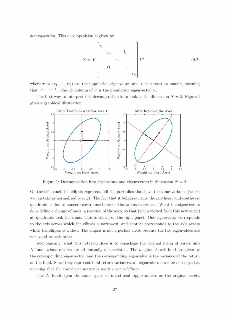
The best way to interpret this decomposition is to look at the dimension N = 2. Figure 1
gives a graphical illustration.
-1.5 -1 -0.5 0 0.5 1 1.5
Weight on First Asset
-1.5
-1
-0.5
0
0.5
1
1.5
Weigh
ton
Secon
dAsset
Set of Portfolios with Variance 1
-1.5 -1 -0.5 0 0.5 1 1.5
Weight on First Asset
-1.5
-1
-0.5
0
0.5
1
1.5
Weigh
ton
Secon
dAsset
After Rotating the Axes
0 0
Figure 1: Decomposition into eigenvalues and eigenvectors in dimension N = 2.
On the left panel, the ellipsis represents all the portfolios that have the same variance (which
we can take as normalized to one). The fact that it bulges out into the northeast and southwest
quadrants is due to nonzero covariance between the two asset returns. What the eigenvectors
do is define a change of basis, a rotation of the axes, so that (when viewed from this new angle)
all quadrants look the same. This is shown on the right panel. One eigenvector corresponds
to the axis across which the ellipsis is narrowest, and another corresponds to the axis across
which the ellipsis is widest. The ellipsis is not a perfect circle because the two eigenvalues are
not equal to each other.
Economically, what this rotation does is to repackage the original menu of assets into
N funds whose returns are all mutually uncorrelated. The weights of each fund are given by
the corresponding eigenvector; and the corresponding eigenvalue is the variance of the return
on the fund. Since they represent fund return variances, all eigenvalues must be non-negative,
meaning that the covariance matrix is positive semi-definite.
The N funds span the same space of investment opportunities as the original assets,
27

therefore we can rewrite equation (9.1) as
wTANGENCY = scalar×N∑
i=1
v′iµ
τivi . (9.3)
Equation (9.3) demonstrates that the tangency portfolio is best viewed not as a combination of
theN original assets, but as a combination of theN uncorrelated eigenvector funds. The capital
assigned to each fund is proportional to its expected return and inversely proportional to its
variance, which makes economic sense.
It is easy to justify that the spectral decomposition is important for portfolio selection.
Consider the hypothetical covariance matrix of monthly stock returns in Table 9.
Apple Boeing Disney IBM
Apple 0.2694 0.5714 0.2900 0.3080
Boeing 0.5714 1.3910 0.6674 0.6964
Disney 0.2900 0.6674 0.3275 0.3433
IBM 0.3080 0.6964 0.3433 0.4822
Table 9: Hypothetical covariance matrix between four US stocks.
To the naked eye, it looks fine. However, its eigenvalues are (0, 0.0299, 0.1072, 2.3329). Even
to the naked eye, the first eigenvalue looks wrong. The tangency portfolio does not exist when
an eigenvalue is equal to zero. This is why extracting eigenvalues and eigenvectors is called
the spectral decomposition: It enables us to penetrate right through the outer appearance of
the matrix into its inner structure.
In practice, we do not know the true covariance matrix Σ, therefore we must use some
estimator of it. It is known that the sample covariance matrix ST ..= Y ′TYT /T is a consistent
estimator of Σ when the sample size T goes to infinity while the dimension N remains
fixed (an often overlooked yet crucial assumption, to which we will return later). Mirroring
equation (9.2), define the spectral composition of ST as
ST =.. UT
λ1,T
λ2,T 0. . .
0. . .
λN,T
U ′T , (9.4)
where λT..= (λ1,T , . . . , λN,T ) are the sample eigenvalues and UT is a rotation matrix
(U ′T = U−1
T ) whose ith column is the sample eigenvector ui,T . An implementable version
28
of equation (9.3) is
wTANGENCY = scalar×N∑
i=1
u′i,Tµ
λi,Tui,T . (9.5)
This formulation leads to a fundamental insight: In the denominator, we have λi,T , which is
the in-sample variance of the ith eigenvector fund ui,T , whereas for investment purposes we
need its out-of-sample variance u′i,TΣui,T instead. The whole point of the procedure advocated
in this paper is to replace the former with (a consistent estimate of) the latter. Investment
decisions are always evaluated out of sample.
One little-known mathematical fact about the eigenvalues is that they are the most
dispersed diagonal elements that can be obtained through rotation; see Ledoit and Wolf (2004b,
Section 2.3). Given that the group of rotations has dimensionality of order N2, the potential for
overfitting is tremendous when N is large. Overfitting causes excess dispersion: The smallest
sample eigenvalues are too small, leading to over-investment, and the largest sample eigenvalues
too large, leading to under-investment. The overall result is mal-investment. This insight goes
a long way towards explaining the observation by Michaud (1989) about “error maximization”.
However, to fix it requires a detour through multivariate statistics.
9.2 Importance of the Eigenvalues for Covariance Matrix Estimation
If we are going to look for estimators that improve upon the sample covariance matrix,
the first task is to decide where to look. We need to specify a class of eligible estimators,
and search within this class for one that beats the sample covariance matrix. In mathematics,
a standard way to approach this kind of problem is to say that we want estimators that
have certain appealing properties. One such property initially championed by Stein (1975)
and subsequently adopted by many other authors is called rotation equivariance. A covariance
matrix estimator ΣT (YT ) is said to be rotation-equivariant if and only if for any N -dimensional
rotation matrix W ,
ΣT (YTW ) =W ′ ΣT (YT )W . (9.6)
That is, the estimate based on the rotated data equals the rotation of the estimate based on
the original data. Absent any a priori knowledge about the orientation of the true eigenvectors,
it is natural to consider only covariance matrix estimators that are rotation-equivariant.
It can be proven that the class of rotation-equivariant estimators that are a function of the
sample covariance matrix is the class of estimators of the form
ΣΨT..= UT
ψ1,T
ψ2,T 0. . .
0. . .
ψN,T
U ′T , (9.7)
29

where ΨT..= (ψ1,T , . . . , ψN,T ) can be any vector in [0,+∞)N ; for example, see Perlman (2007,
Section 5.4). Thus, we preserve the sample eigenvectors, but are free to modify the sample
eigenvalues in any way needed to improve upon the sample covariance matrix. Given Section
9.1, the basic idea will be to set ψi,T equal to u′i,TΣui,T , or if it is unavailable (the more likely
scenario, given that it depends on the population covariance matrix, which is unobservable), a
consistent estimator thereof.
In summary, the key intuition is that we have to preserve the sample eigenvectors because
we lack a priori information about the orientation of the true eigenvectors, and the goal is
to modify the sample eigenvalues so we can beat the sample covariance matrix.
9.3 General Asymptotics
As mentioned before, the sample covariance matrix ST is a consistent estimator of the
population covariance matrix Σ when the sample size T goes to infinity while the dimension N
remains fixed. This is strange: why is T allowed to move but not N? When we have five years
of daily data (T = 1250) on the components of the Russell 1000 stock index (N = 1000), it is
easy to believe that T goes to infinity, as 1250 is a large number by any measure in statistics,
but who is to say that N is finite? Shouldn’t numbers that go to infinity be much bigger than
those that are assumed to remain finite?
The answer is to simply relax the constraining assumption that N is fixed and instead
allow the dimension to move along with the sample size: N ..= N(T ). This is called general
asymptotics, large-dimensional asymptotics, or Kolmogorov asymptotics. Notation-wise, this
kind of asymptotics requires appending the subscript T to the population covariance matrix,
and also its eigenvalues and eigenvectors, a convention that we will uphold from here onwards.
Given that the number of eigenvalues N goes to infinity, it is no longer possible to make
statements about individual eigenvalues. This is why it is necessary to introduce what is
known as spectral distributions. The population and sample spectral distributions are defined
respectively as
∀x ∈ R HT (x) ..=1
N
N∑
i=1
1{x≤τi,T } (9.8)
∀x ∈ R FT (x) ..=1
N
N∑
i=1
1{x≤λi,T } , (9.9)
where 1 denotes the indicator function. The spectral distribution can be interpreted as a cross-
sectional cumulative distribution function (c.d.f.): it is a nondecreasing function having values
between zero and one that returns the proportion of eigenvalues lower than its argument.
Two standard assumptions under general asymptotics are (i) that the population spectral
distribution converges to a well-defined limit H called the limiting spectral distribution and
30

(ii) that the ratio N/T converges to a finite limit c called the concentration:
HT (x) −→ H(x) at all points of continuity of H (9.10)
N
T−→ c < +∞ . (9.11)
Along with other technical assumptions that can vary from author to author, these two
assumptions imply the fundamental result of general asymptotics, which is that the sample
spectral distribution converges to a nonrandom limit F called the limiting spectral distribution:
FT (x)a.s.−→ F (x) at all points of continuity of F . (9.12)
Remark 9.1. The fact that the matrix is random but its eigenvalues are not is a
remarkable mathematical phenomenon first discovered by Wigner (1955) while investigating
the properties of the wave functions of complicated quantum mechanical systems; see Figure 2
for an illustration of this influential result.
Figure 2: The eigenvalues of a large Wigner matrix follow Wigner’s semi-circular law. Wigner
matrices are random symmetric matrix with i.i.d. standard normal entries. (They are different
from covariance matrices.) This picture does not represent an average across Monte Carlo
simulations: it is just the result of one single draw.
The limiting sample spectral distribution F is the key to knowing where the sample
eigenvalues lie. There are a few things we can immediately say about this important object:
(a) F is uniquely determined by H and c; see Silverstein and Choi (1995)
(b) F = H ⇐⇒ c = 0
(c)∫ +∞−∞ x dF (x) =
∫ +∞−∞ x dH(x)
31

(d)∫ +∞−∞ x2 dF (x) =
∫ +∞−∞ x2 dH(x) + c
[∫ +∞−∞ x dH(x)
]2
Statement (b) confirms that finite-dimensional asymptotics are included as a special case of
general asymptotics. When N remains fixed and finite, N/T converges to zero as T goes
to infinity. In this case, the eigenvalues of the sample covariance matrix are consistent
estimators of their population counterparts. This remains true even if N goes to infinity
along with T , as long as it grows sufficiently slowly (say in log(T ) or√T ). When c = 0 or,
practically speaking, when N/T is minuscule, the sample covariance matrix works fine.
For five years of history on the Russell 1000, the ratio N/T is equal to 0.8, so it is definitely
not minuscule. c > 0 is the relevant case for all large covariance matrices, because when N
is large it is very difficult to have a sample size such that the ratio is N/T minuscule. In
this case, the sample eigenvalues never get close to their population counterparts, so we
enter a qualitatively different regime where improvement over the sample covariance matrix
is possible.
Statement (c) means that the cross-sectional average of the sample eigenvalues is in the
right place even when c > 0: it never needs fixing. However, Statement (d) shows their
cross-sectional dispersion around the average is systematically inflated, and excess dispersion
increases in c; see Yin (1986, Equation (4.14)). This confirms formally the intuition developed
at the end of Section 9.1. To fix this problem, the filtering applied to sample eigenvalues
will have to ‘shrink’ their cross-sectional dispersion towards the center; see Ledoit and Wolf
(2004b).
9.4 Single Mass Point
One way to get information about the limiting sample spectral distribution is to study what
happens in the simplest case, when the population covariance matrix ΣT is equal to the identity
matrix. In this case, a closed-form solution exists: F is differentiable, and its derivative f , called
the limiting spectral density, follows the so-called Marcenko-Pastur Law:
∀x ∈ [a, b] f(x) ..=
√(b− x)(x− a)
2πcx,
where the bounds of the support of f are a ..= (1 −√c)2 and b ..= (1 +
√c)2 respectively; see
Marcenko and Pastur (1967).
32

0 0.5 1 1.5 2 2.5 3Sample Eigenvalues
0
0.5
1
1.5
2
2.5
3
3.5
Lim
itingSpectralDen
sity
Marcenko-Pastur Law
c = 1/100c = 1/10c = 1/2
Figure 3: Limiting cross-sectional density of sample eigenvalues for various concentration levels.
Some lessons can be drawn, that reinforce and complement what we have learned from the first
two moments:
1. Sample eigenvalues are smudged to the left and the right of the population eigenvalues.
2. The amount of excess spread increases in the concentration ratio c.
3. The smallest sample eigenvalues are too small, the largest ones too large.
4. This systematic bias must be filtered out by shrinking the distribution of sample
eigenvalues towards the center.
5. The center (cross-sectional average) of the sample eigenvalues distribution is accurate:
it matches its population counterpart.
6. The density is right-skewed: there are many small sample eigenvalues and few large ones.
7. It is only in the limit c → 0 that sample eigenvalues start to conform with standard
(fixed-dimension) asymptotics.
The concentration c needs to be very close to 0 before concerns about excess dispersion can
be safely dismissed. For c = 1/10, meaning that we have 10 times more observations than
variables, which many people would deem sufficient, some sample eigenvalues are still less than
half their population counterparts. Even when c = 1/100, out-of-sample portfolio variances
can be under/overestimated by 20%, inducing over/under-allocation of risk capital by the same
percentage.
9.5 Two Mass Points
These seven observations carry over to the case where a fraction α of the population eigenvalues
are equal to one, while the rest are equal to some τ > 1. The behavior of the limiting spectral
density is pretty much as one would expect intuitively: There are two clusters formed around
33
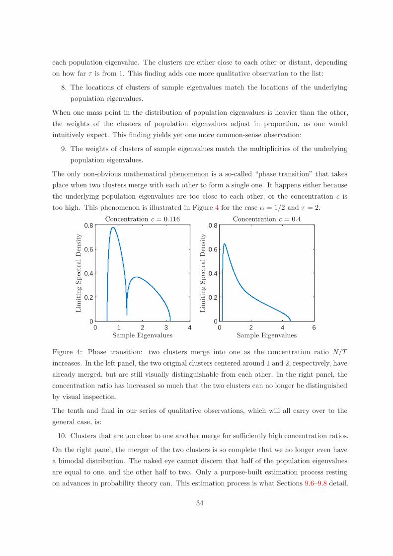
each population eigenvalue. The clusters are either close to each other or distant, depending
on how far τ is from 1. This finding adds one more qualitative observation to the list:
8. The locations of clusters of sample eigenvalues match the locations of the underlying
population eigenvalues.
When one mass point in the distribution of population eigenvalues is heavier than the other,
the weights of the clusters of population eigenvalues adjust in proportion, as one would
intuitively expect. This finding yields yet one more common-sense observation:
9. The weights of clusters of sample eigenvalues match the multiplicities of the underlying
population eigenvalues.
The only non-obvious mathematical phenomenon is a so-called “phase transition” that takes
place when two clusters merge with each other to form a single one. It happens either because
the underlying population eigenvalues are too close to each other, or the concentration c is
too high. This phenomenon is illustrated in Figure 4 for the case α = 1/2 and τ = 2.
0 1 2 3 4Sample Eigenvalues
0
0.2
0.4
0.6
0.8
Lim
itingSpectralDen
sity
Concentration c = 0.116
0 2 4 6Sample Eigenvalues
0
0.2
0.4
0.6
0.8
Lim
itingSpectralDen
sity
Concentration c = 0.4
Figure 4: Phase transition: two clusters merge into one as the concentration ratio N/T
increases. In the left panel, the two original clusters centered around 1 and 2, respectively, have
already merged, but are still visually distinguishable from each other. In the right panel, the
concentration ratio has increased so much that the two clusters can no longer be distinguished
by visual inspection.
The tenth and final in our series of qualitative observations, which will all carry over to the
general case, is:
10. Clusters that are too close to one another merge for sufficiently high concentration ratios.
On the right panel, the merger of the two clusters is so complete that we no longer even have
a bimodal distribution. The naked eye cannot discern that half of the population eigenvalues
are equal to one, and the other half to two. Only a purpose-built estimation process resting
on advances in probability theory can. This estimation process is what Sections 9.6–9.8 detail.
34

9.6 Limiting Sample Spectral Distribution
In what follows, we describe only the case 0 < c < 1. The case c = 0 is excluded because it is
trivial: The sample eigenvalues converge to their population counterparts, and the sample
covariance matrix is optimal. The case c ≥ 1 is excluded because it would render the
exposition less fluid, but it poses no great difficulty and can be dealt with just as effectively;
see Ledoit and Wolf (2017a). One convenience that the assumption 0 < c < 1 buys us is that
the limiting sample spectral distribution admits a countinuous derivative f .
In order to relate F to H quantitatively, a new mathematical object must be introduced:
the Stieltjes (1894) transform. The Stieltjes transform of the distribution function F is defined
on the half-plane of complex numbers with strictly positive imaginary part C+ by
∀z ∈ C+ mF (z) ..=
∫ +∞
−∞
1
λ− zdF (λ) . (9.13)
Although it is difficult to visualize a complex function, there is an important result valid
specifically for F that will help us gain an intuitive understanding of its Stieltjes transform.
Indeed, F is smooth enough for the limit
limz∈C+→x
mF (z) =.. mF (x) (9.14)
to exist for all x ∈ R. mF extends the Stieltjes transform from the upper half of the complex
plane onto the real line. Now mF , being a complex-valued function of real argument, is much
easier to comprehend. In particular, its imaginary part is simply the limiting spectral density f
divided by π. Thus, if we have mF , we get the density f and then also the distribution F
(by integration of f). The quantiles of F tell us where the sample eigenvalues are located in
the limit.
mF can be deduced from H in only one known way, which is the following. For all x ∈ R,
m ..= mF (x) is the unique solution in C+ to the equation
m =
∫ +∞
−∞
1
τ[1− c− c xm
]− x
dH(τ) (9.15)
Equation (9.15) is the fundamental building block of all research in large-dimensional
covariance matrix estimation. Although it may look daunting, and indeed there is generally
no closed-form solution, it can be solved numerically in a matter of seconds for N = 1000
eigenvalues; see Ledoit and Wolf (2017b). This equation has been around for half a century
in some form or other, and all researchers in the field are fully confident that “it does
exactly what it says on the tin”, even though it is difficult to provide intuitive insight; see
Marcenko and Pastur (1967), Silverstein and Bai (1995), Silverstein (1995), as well as the
authoritative monograph by Bai and Silverstein (2010).
F is smooth, it is more spread out than H, and the excess spread increases in c. In the limit,
as c → 0, we can recognize on the right-hand side the Stieltjes transform of H, so F becomes
35
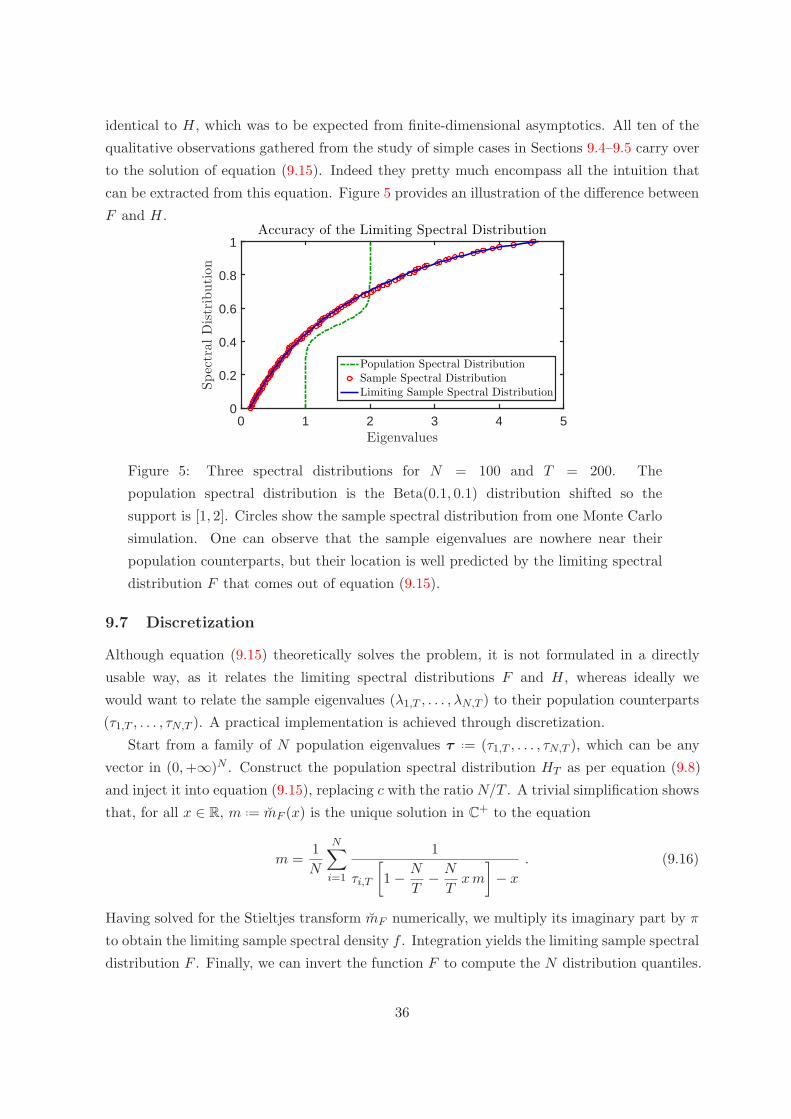
identical to H, which was to be expected from finite-dimensional asymptotics. All ten of the
qualitative observations gathered from the study of simple cases in Sections 9.4–9.5 carry over
to the solution of equation (9.15). Indeed they pretty much encompass all the intuition that
can be extracted from this equation. Figure 5 provides an illustration of the difference between
F and H.
0 1 2 3 4 5Eigenvalues
0
0.2
0.4
0.6
0.8
1
SpectralDistribution
Accuracy of the Limiting Spectral Distribution
Population Spectral DistributionSample Spectral DistributionLimiting Sample Spectral Distribution
Figure 5: Three spectral distributions for N = 100 and T = 200. The
population spectral distribution is the Beta(0.1, 0.1) distribution shifted so the
support is [1, 2]. Circles show the sample spectral distribution from one Monte Carlo
simulation. One can observe that the sample eigenvalues are nowhere near their
population counterparts, but their location is well predicted by the limiting spectral
distribution F that comes out of equation (9.15).
9.7 Discretization
Although equation (9.15) theoretically solves the problem, it is not formulated in a directly
usable way, as it relates the limiting spectral distributions F and H, whereas ideally we
would want to relate the sample eigenvalues (λ1,T , . . . , λN,T ) to their population counterparts
(τ1,T , . . . , τN,T ). A practical implementation is achieved through discretization.
Start from a family of N population eigenvalues τ ..= (τ1,T , . . . , τN,T ), which can be any
vector in (0,+∞)N . Construct the population spectral distribution HT as per equation (9.8)
and inject it into equation (9.15), replacing c with the ratio N/T . A trivial simplification shows
that, for all x ∈ R, m ..= mF (x) is the unique solution in C+ to the equation
m =1
N
N∑
i=1
1
τi,T
[1− N
T− N
Txm
]− x
. (9.16)
Having solved for the Stieltjes transform mF numerically, we multiply its imaginary part by π
to obtain the limiting sample spectral density f . Integration yields the limiting sample spectral
distribution F . Finally, we can invert the function F to compute the N distribution quantiles.
36

This is exactly how the QuEST function is constructed. It maps an N -dimensional vector τ
of population eigenvalues into another N -dimensional vector(q1N,T (τ ), q
2N,T (τ ), . . . , q
NN,T (τ )
),
which represents a deterministic equivalent of the sample eigenvalues, by discretizing equation
(9.15). The output (quantiles of F ) can be interpreted as the expectation of the sample eigen-
values, although this correspondence is rigorous only in the large-dimensional asymptotic limit.
9.8 Recovering Population Eigenvalues
As can be gathered from the above exposition, it is more straightforward to go from population
to sample eigenvalues than the other way around. This is an intrinsic feature of equation (9.15),
which is our only tractable hook into the underlying mathematical truth.
However, given that equation (9.15) has been made more practical through discretization
inside the QuEST function as seen in Section 9.7, inverting it becomes a simple numerical
problem. Find the vector τ ∈ (0,+∞)N such that the function’s output(q1N,T (τ ), q
2N,T (τ ), . . . ,
qNN,T (τ ))matches most closely the observed sample eigenvalues (λ1,T , . . . , λN,T ). Any capable
off-the-shelf nonlinear optimizer can solve this problem. Two recommended optimizers are
Stanford Business Software’s SNOPT and Matlab’s fmincon; they both can easily handle
dimensions up to N = 1000 within a reasonable amount of time, a few minutes at most. In a
nutshell, the problem of recovering the population eigenvalues from the sample eigenvalues has
been resolved by numerically inverting the multivariate function that discretizes equation (9.15).
Figure 6 illustrates the accuracy of this procedure.
0 200 400 600 800 1000Index of Eigenvalues
0
2
4
6
8
10
Pop
ulation
Eigenvalues
Accuracy of Eigenvalues Estimator
EstimatedTrue
Figure 6: The matrix dimension is N = 1000 and the sample size is T = 3000. This graph
is based on a single Monte Carlo simulation. Numerically inverting the discretized version of
equation (9.15) asymptotically recovers the population eigenvalues.
37

9.9 Nonlinear Shrinkage
At this juncture, it might be tempting to conclude that replacing the observed sample
eigenvalues with the estimated population eigenvalues that come from inverting the QuEST
function yields the optimal estimator of the covariance matrix. However this is not
the case. The population eigenvalues (or consistent estimators thereof) are only optimal when
recombined with the population eigenvectors. The latter are unobservable and, unlike the
eigenvalues, there is no hope of recovering them through some advanced mathematics. The
reason is that they live in a space of dimension N(N − 1)/2, which is infinitely too large given
that we only collect N × T noisy data points, T being of the same order of magnitude as N .
In the terminology of Section 9.1, we do not want λi,T , the in-sample variance of the sample
eigenvector ui,T ; but we also do not want τi,T , the out-sample variance of the population
eigenvector vi,T . This is because we do not have vi,T . What we want is a hybrid: u′i,TΣui,T ,
the out-sample variance of the sample eigenvector ui,T . This quantity is estimated consistently
under general asymptotics by the following “nonlinear shrinkage” formula:
u′i,TΣui,T ≈ λi,T∣∣∣∣1−N
T− N
Tλi,T mF (λi,T )
∣∣∣∣2 , (9.17)
where | · | denotes the modulus of a complex number, and mF is the function defined in (9.16);
see Ledoit and Peche (2011, Theorem 3). Similar to equation (9.15), it is hard to give intuition:
this is just what comes out of the underlying mathematics. We are fortunate to have any explicit
equation at all; it basically comes from a generalization of equation (9.15). Extensive Monte
Carlo simulations confirm the accuracy of this formula; see Ledoit and Wolf (2012, Section 6).
One can see that when N/T is negligible, there is a negligible amount of shrinkage, as expected
from finite-dimensional asymptotics.
Calling the right-hand side ψi,T and injecting it into equation (9.7) yields an estimator of
the covariance matrix that improves upon the sample covariance matrix when the dimension N
is not negligible with respect to the sample size T . A graphical illustration is given in Figure 7.
38

1 1.5 2 2.5Sample Eigenvalues
1
1.5
2
2.5
Concentration ratio c = 1/10
Nonlinearly Shrunk EigenvaluesPopulation Eigenvalues
Figure 7: Nonlinearly shrunk eigenvalues as a function of sample eigenvalues. The
population eigenvalues come from the Beta(0.1, 0.1) distribution, shifted so the
support is [1, 2]. The optimal shrinkage transformation is highly nonlinear. The
population eigenvalues are also plotted for reference as the dashed line. They are not
the same as the shrunk eigenvalues, and are more spread out.
To summarize, the overall procedure consists of three consecutive steps:
Step 1 Given the sample eigenvalues (λ1,T , . . . , λN,T ), invert the QuEST function defined in
Section 9.7 to obtain consistent estimates of the population eigenvalues;
Step 2 Plug the (estimated) population eigenvalues into equation (9.16) to compute the
complex-valued function mF ;
Step 3 Replace the sample eigenvalues with the nonlinear shrinkage formula on the right-hand
side of equation (9.17), while preserving the sample eigenvectors.
All of this is handled automatically by the QuEST software, available from the university
faculty website of Michael Wolf. Ledoit and Wolf (2017a) prove that the resulting covariance
matrix estimator is optimal for portfolio selection under general asymptotics within the
rotation-equivariant class.
39
References
Aielli, G. P. (2013). Dynamic conditional correlation: on properties and estimation. Journal
of Business & Economic Statistics, 31(3):282–299.
Bai, Z. D. and Silverstein, J. W. (2010). Spectral Analysis of Large-Dimensional Random
Matrices. Springer, New York, second edition.
Bollerslev, T. (1990). Modeling the coherence in short-run nominal exchange rates: a
multivariate generalized ARCH model. Review of Economics and Statistics, 72:498–505.
Capon, J. (1969). High-resolution frequency-wavenumber spectrum analysis. Proceedings of
the IEEE, 57(8):1408–1418.
DeMiguel, V., Garlappi, L., and Uppal, R. (2009). Optimal versus naive diversification: How
inefficient is the 1/N portfolio strategy? Review of Financial Studies, 22:1915–1953.
El Karoui, N. (2008). Spectrum estimation for large dimensional covariance matrices using
random matrix theory. Annals of Statistics, 36(6):2757–2790.
Engle, R. F. (1982). Autoregressive conditional heteroskedasticity with estimates of the
variance of United Kingdom inflation. Econometrica, 50:987–1007.
Engle, R. F. (2002). Dynamic conditional correlation: A simple class of multivariate generalized
autoregressive conditional heteroskedasticity models. Journal of Business & Economic
Statistics, 20(3):339–350.
Engle, R. F. (2009). Anticipating Correlations: A New Paradigm for Risk Management.
Princeton University Press.
Engle, R. F. and Colacito, R. (2006). Testing and valuing dynamic correlations for asset
allocation. Journal of Business and Economic Statistics, 24(2):238–253.
Engle, R. F. and Kroner, K. (1995). Multivariate simultaneous GARCH. Econometric Theory,
11:122–150.
Engle, R. F. and Mezrich, J. (1996). GARCH for groups. Risk, 9:36–40.
Hafner, C. M. and Reznikova, O. (2012). On the estimation of dynamic conditional correlation
models. Computational Statistics & Data Analysis, 56(11):3533–3545.
Hamilton, J. D. (1994). Time Series Analysis. Princeton University Press, Princeton, NJ.
Haugen, R. A. and Baker, N. L. (1991). The efficient market inefficiency of capitalization-
weighted stock portfolios. The Journal of Portfolio Management, 17(3):35–40.
40
IPCC (2007). Climate change 2007: the scientific basis. In Solomon, S., Qin, D., Manning, M.,
Marquis, M., Averyt, K., Tignor, M. M., Miller, H. L., and Chen, Z., editors, Contribution
of Working Group I to the Fourth Assessment Report of the Intergovernmental Panel on
Climate Change. Cambridge University Press, Cambridge, United Kingdom and New York,
NY, USA. 996pp.
Jagannathan, R. and Ma, T. (2003). Risk reduction in large portfolios: Why imposing the
wrong constraints helps. Journal of Finance, 54(4):1651–1684.
Jegadeesh, N. and Titman, S. (1993). Returns to buying winners and selling losers: Implications
for stock market efficiency. The Journal of Finance, 48(1):65–91.
Ledoit, O. and Peche, S. (2011). Eigenvectors of some large sample covariance matrix ensembles.
Probability Theory and Related Fields, 150(1–2):233–264.
Ledoit, O. and Wolf, M. (2004a). Honey, I shrunk the sample covariance matrix. Journal of
Portfolio Management, 30(4):110–119.
Ledoit, O. and Wolf, M. (2004b). A well-conditioned estimator for large-dimensional covariance
matrices. Journal of Multivariate Analysis, 88(2):365–411.
Ledoit, O. and Wolf, M. (2008). Robust performance hypothesis testing with the Sharpe ratio.
Journal of Empirical Finance, 15:850–859.
Ledoit, O. and Wolf, M. (2011). Robust performance hypothesis testing with the variance.
Wilmott Magazine, September:86–89.
Ledoit, O. and Wolf, M. (2012). Nonlinear shrinkage estimation of large-dimensional covariance
matrices. Annals of Statistics, 40(2):1024–1060.
Ledoit, O. and Wolf, M. (2015). Spectrum estimation: a unified framework for covariance
matrix estimation and PCA in large dimensions. Journal of Multivariate Analysis,
139(2):360–384.
Ledoit, O. and Wolf, M. (2017a). Nonlinear shrinkage of the covariance matrix for portfolio
selection: Markowitz meets Goldilocks. Review of Financial Studies. Forthcoming.
Ledoit, O. and Wolf, M. (2017b). Numerical implementation of the QuEST function. Working
Paper ECON 215, Department of Economics, University of Zurich.
Marcenko, V. A. and Pastur, L. A. (1967). Distribution of eigenvalues for some sets of random
matrices. Sbornik: Mathematics, 1(4):457–483.
Markowitz, H. (1952). Portfolio selection. Journal of Finance, 7:77–91.
41

Mestre, X. (2008). On the asymptotic behavior of the sample estimates of eigenvalues and eigen-
vectors of covariance matrices. IEEE Transactions on Signal Processing, 56(11):5353–5368.
Michaud, R. (1989). The Markowitz optimization enigma: Is optimized optimal? Financial
Analysts Journal, 45:31–42.
Nielsen, F. and Aylursubramanian, R. (2008). Far from the madding crowd — Volatility
efficient indices. Research insights, MSCI Barra.
Pakel, C., Shephard, N., Sheppard, K., and Engle, R. F. (2014). Fitting vast dimensional
time-varying covariance models. Technical report.
Perlman, M. D. (2007). STAT 542: Multivariate Statistical Analysis. University of Washington
(On-Line Class Notes), Seattle, Washington.
Silverstein, J. W. (1995). Strong convergence of the empirical distribution of eigenvalues of
large-dimensional random matrices. Journal of Multivariate Analysis, 55:331–339.
Silverstein, J. W. and Bai, Z. D. (1995). On the empirical distribution of eigenvalues of a class
of large-dimensional random matrices. Journal of Multivariate Analysis, 54:175–192.
Silverstein, J. W. and Choi, S. I. (1995). Analysis of the limiting spectral distribution of
large-dimensional random matrices. Journal of Multivariate Analysis, 54:295–309.
Stein, C. (1975). Estimation of a covariance matrix. Rietz lecture, 39th Annual Meeting IMS.
Atlanta, Georgia.
Stieltjes, T. J. (1894). Recherches sur les fractions continues. Annales de la Faculte des
Sciences de Toulouse 1re Serie, 8(4):J1–J122.
Wigner, E. P. (1955). Characteristic vectors of bordered matrices with infinite dimensions.
Annals of Mathematics, 62(3):548–564.
Yin, Y. (1986). Limiting spectral distribution for a class of random matrices. Journal of
Multivariate Analysis, 20(1):50–68.
Zumbach, G. O. (2007). The RiskMetrics 2006 methodology. Technical report, RiskMetrics
Group. Available at https://ssrn.com/abstract=1420185.
42