Land-sea interactions underclimate change

NMA Summer Course 2009Climate Impacts on the Baltic Sea – From Science to Policy

Ben Smith

Geobiosphere Science Centre,Lund University, Sweden

www.nateko.lu.se/embers

• The Baltic Sea catchment area and land-sea biogeochemical links

• Terrestrial ecosystems are changing in response to climate change! What are the underlying processes and mechanisms?

• Modelling vegetation and ecosystem response to climate and CO2 –some future projections

• Land use change! Can we develop plausible future scenarios?

Lecture 15-16.30

Future scenario modelling exercise 17-18.30

Plan for the afternoon

• We will work with LPJ-GUESS, a model that simulates vegetation and ecosystem changes in response to climate change

• Formulate and address a question regarding potential future changes in Baltic catchment ecosystems

• Present results with policy implications in a 5-minute presentation

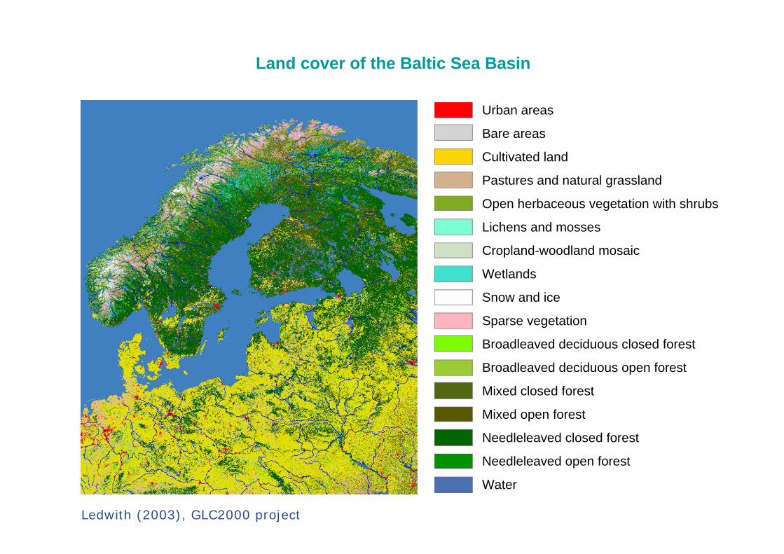
Urban areas

Bare areas

Cultivated land

Pastures and natural grassland

Open herbaceous vegetation with shrubs

Lichens and mosses

Cropland-woodland mosaic

Wetlands

Snow and ice

Sparse vegetation

Broadleaved deciduous closed forest

Broadleaved deciduous open forest

Mixed closed forest

Mixed open forest

Needleleaved closed forest

Needleleaved open forest

Water

Land cover of the Baltic Sea Basin

Ledwith (2003), GLC2000 project

Urban areas

Bare areas

Cultivated land

Pastures and natural grassland

Open herbaceous vegetation with shrubs

Lichens and mosses

Cropland-woodland mosaic

Wetlands

Snow and ice

Sparse vegetation

Broadleaved deciduous closed forest

Broadleaved deciduous open forest

Mixed closed forest

Mixed open forest

Needleleaved closed forest

Needleleaved open forest

Water

Land cover of the Baltic Sea Basin

Urban areas

Bare areas

Cultivated land

Pastures and natural grassland

Open herbaceous vegetation with shrubs

Lichens and mosses

Cropland-woodland mosaic

Wetlands

Snow and ice

Sparse vegetation

Broadleaved deciduous closed forest

Broadleaved deciduous open forest

Mixed closed forest

Mixed open forest

Needleleaved closed forest

Needleleaved open forest

Water

Land cover of the Baltic Sea Basin

Urban areas

Bare areas

Cultivated land

Pastures and natural grassland

Open herbaceous vegetation with shrubs

Lichens and mosses

Cropland-woodland mosaic

Wetlands

Snow and ice

Sparse vegetation

Broadleaved deciduous closed forest

Broadleaved deciduous open forest

Mixed closed forest

Mixed open forest

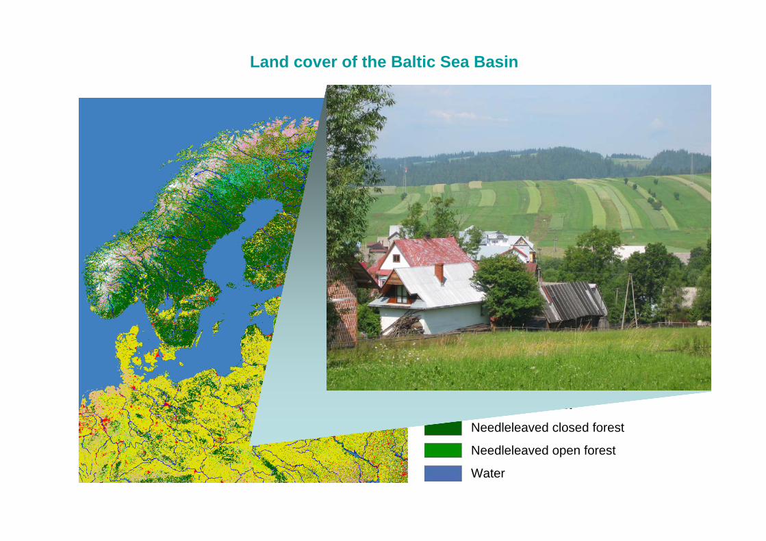
Needleleaved closed forest

Needleleaved open forest

Water

Land cover of the Baltic Sea Basin

Urban areas

Bare areas

Cultivated land

Pastures and natural grassland

Open herbaceous vegetation with shrubs

Lichens and mosses

Cropland-woodland mosaic

Wetlands

Snow and ice

Sparse vegetation

Broadleaved deciduous closed forest

Broadleaved deciduous open forest

Mixed closed forest

Mixed open forest

Needleleaved closed forest

Needleleaved open forest

Water

Land cover of the Baltic Sea Basin

0.0

0.1

0.2

0.3

0.4

% arable land

0.0

0.1

0.2

0.0

0.5

1.0

1.5

2.0

N losses modelledN losses measured

% arable landP losses modelledP losses measured

1987 1989 1991 1993 1995 1997

kgP

ha−1

yr−1

0

10

20

30

0

1

2

3

0

20

40

60

1987 1989 1991 1993 1995 1997

0

10

20

30

40

0

5

10

15

0

20

40

60

80

Whole catchment

Upper course

Vända ditch

kgN

ha−

1yr

−1

0

10

20

30

40

0

5

10

15

0

20

40

60

80

Whole catchment

Upper course

Vända ditch

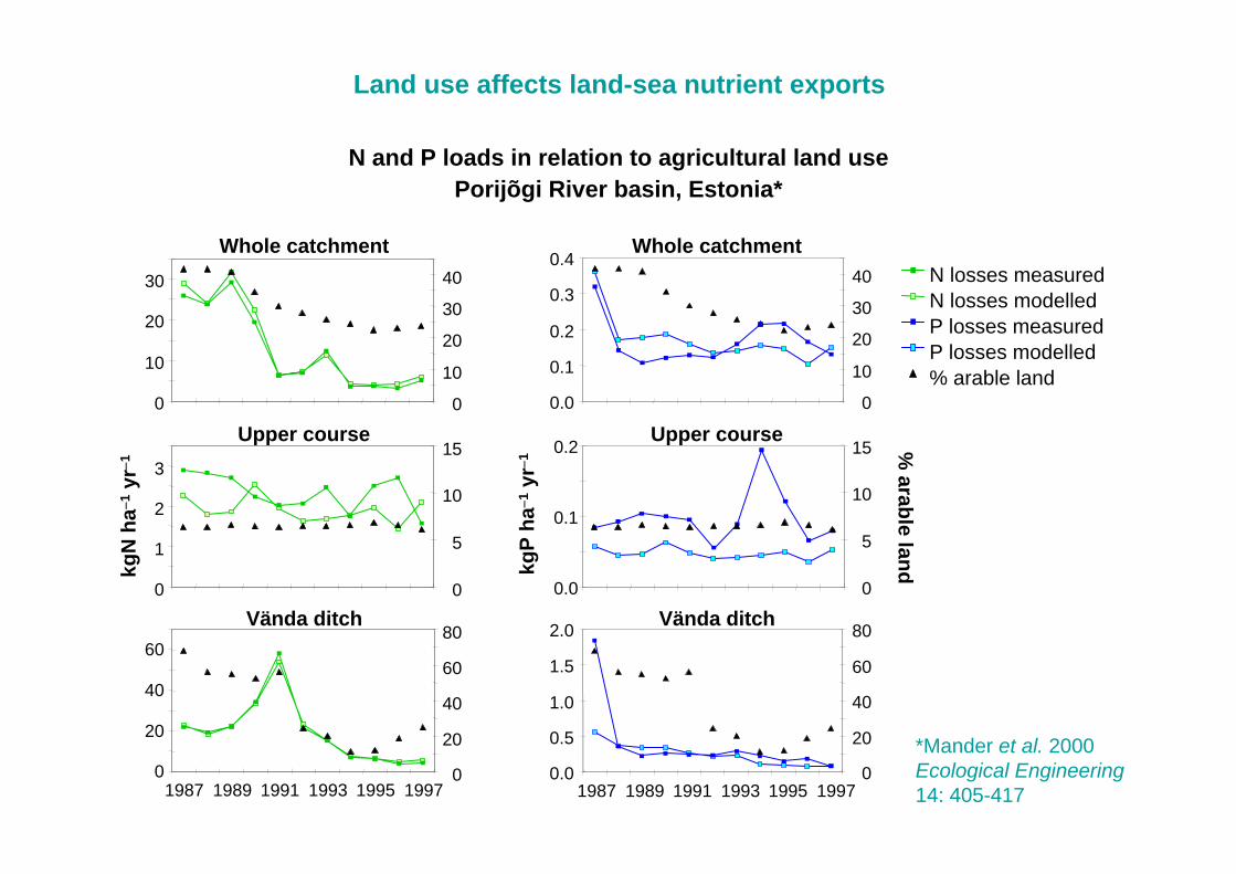
Land use affects land-sea nutrient exports

N and P loads in relation to agricultural land usePorijõgi River basin, Estonia*

*Mander et al. 2000Ecological Engineering14: 405-417

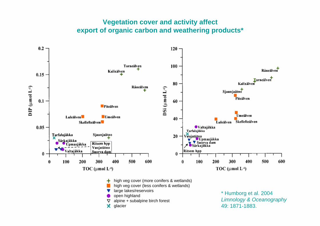
high veg cover (more conifers & wetlands)high veg cover (less conifers & wetlands)large lakes/reservoirsopen highlandalpine + subalpine birch forestglacier

Vegetation cover and activity affectexport of organic carbon and weathering products*

* Humborg et al. 2004Limnology & Oceanography49: 1871-1883.

*Tucker et al. 2001. International Journalof Biometeorology 45: 184

Change in land surface greenness(NDVI) 1982-1999*

increasing ’greenness’ →

Increased greenness at mid-high northern latitudes– effect of a longer growing season?

Year

biom

ass

(t m

−3)

leaves and needles

roots

stems and branches

Changed biomass allocation in Russian forests*– response to higher temperatures, or increased rainfall?

*Lapenis et al. 2005.Global Change Biology 11: 2090-2102.

Trends in 644 plant phenological time seriesfrom Estonia 1948-1999*

non-significant trend

significant trend

*Ahas & Aasa 2006International Journal of Biometeorology51: 17-26

Changing phenology– earlier spring and summer phases over last 50 years

*Walther et al. 2005.Proceedings of the Royal Society B 272: 1427

former distribution

modelled recentdistribution

recent observation

0°C January isotherm

1931-1960 1981-2000

Some species are changing their distributionsto keep track with shifting climate zones

Range shift in holly, Ilex aquifolium*

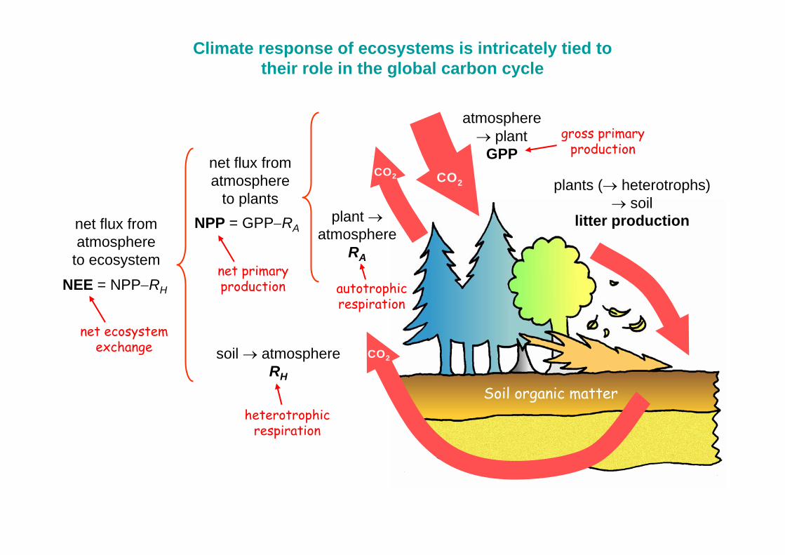
atmosphere→ plant

GPP

plants (→ heterotrophs)→ soil

litter production

soil → atmosphereRH

plant →atmosphere

RA

net flux fromatmosphere

to plants

Soil organic matter

NPP = GPP−RAnet flux fromatmosphere

to ecosystem

NEE = NPP−RH

Climate response of ecosystems is intricately tied totheir role in the global carbon cycle

CO2CO2

CO2

net ecosystemexchange

net primaryproduction

gross primaryproduction

heterotrophicrespiration

autotrophicrespiration

Photosynthesis

CO2 + H2O + PAR CH2O + O2

rubiscoN-rich enzyme

Net reaction of photosynthesis

sunlight carbohydrate

• Carried out by autotrophs, mainly land plants and algae

• Source of virtually all biomass and energy for life processes of living organisms

• Source of oxygen in the atmosphere

• Depends on availability of light energy in usable wavelenths (photosynthetically-active radiation, PAR) and the chemical ingredients CO2 and water

• Rate-limiting step – carboxylation – catalysed by rubisco, an enzyme which accounts for ∼ 50% of all organically-bound nitrogen

• Gross primary production (GPP) = sum of all photosynthesis in ecosystem over a given period of time (usually 1 year)

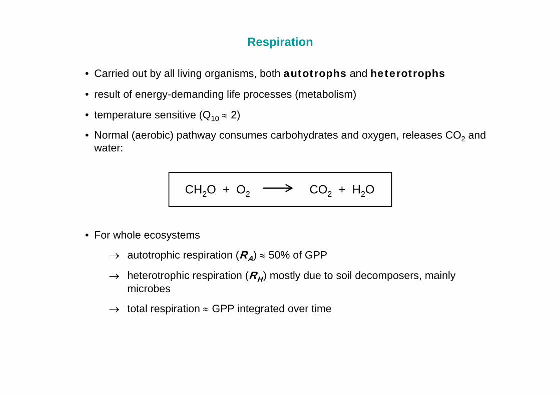
Respiration

• Carried out by all living organisms, both autotrophs and heterotrophs

• result of energy-demanding life processes (metabolism)

• temperature sensitive (Q10 ≈ 2)

• Normal (aerobic) pathway consumes carbohydrates and oxygen, releases CO2 and water:

CH2O + O2 CO2 + H2O

• For whole ecosystems

→ autotrophic respiration (RA) ≈ 50% of GPP

→ heterotrophic respiration (RH) mostly due to soil decomposers, mainly microbes

→ total respiration ≈ GPP integrated over time

C-allocation

LAI

shading

transpiration

evaporation

root competition

stomatalconductance

soil respiration

N-mineralisationsoil water

T

Aphotosynthesis

plant respiration

T

RA

NPP

NEE

Ecosystem processes affected by a change in temperature

litteramount +quality

leaf area index= leaf area / ground area

Warming experimentsinvestigate effects of increased temperatures on whole ecosystems*

-3

-2

-1

0

1

2

3

soilwater

soilrespiration

N mineral-isation

NPP

Sta

ndar

dise

d m

ean

diffe

renc

e

increase

decrease

Relative effect of warming(mean of 20 studies)

Warming experimentToolik Lake, Alaska

* Rustad et al. 2001Oecologia 126: 543-562

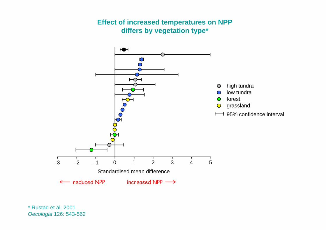
−3 −2 −1 0 1 2 3 4 5

Standardised mean difference

high tundralow tundraforestgrassland95% confidence interval

increased NPPreduced NPP

Effect of increased temperatures on NPPdiffers by vegetation type*

* Rustad et al. 2001Oecologia 126: 543-562

H2O

CO2

H2O

CO2

high CO2 concentration – reducedstomatal conductance limits H2O loss

low CO2 concentrationat leaf surface

Higher CO2 concentrations improve water use efficiency (WUE*)of photosynthesis

*WUE =CO2 assimilation in photosynthesis

H2O loss via transpiration

Stomata optimiseCO2 uptake againstH2O loss

NPP in ambient CO2 (gC m−2 yr−1)

NP

P in

ele

vate

d C

O2

(gC

m−2

yr−1

)

25% greater NPP under 550 ppm CO2independent of tree species and site

Forest FACE experimentin North Carolina

Free-air CO2-enrichment (FACE) experimentssuggest that rising CO2 concentrations will enhance NPP*

* Norby et al. 2005Proceedings of theNational Academy of Sciences USA102: 18052-18056

substrate C:N = 300

consumptionby microbes

respirationCO2

microbesC:N = 10

mineral N pool- lost to plants

immobilisation

Decomposition of low quality (high C:N)substrate immobilises N

substrate C:N = 30consumptionby microbes

respirationCO2

microbesC:N = 10

mineralised N- available to plants

miner-alisation

Decomposition of high quality (low C:N)substrate leads to net mineralisation of N

Will litter from high-CO2 vegetation immobilise N? *

*Luo et al. 2004BioScience 54: 731-740

field expts

ecosystem fluxstudies

satellites

lab expts

fieldmonitoringstudies

chloroplast,mitochondrion

resp

onse

dis

tanc

e (1

0ym

)

response time (10x years)1 sec 1 hour1 min 1 day 1 year 100 years 10,000 years

treeseedling

stomate

adulttree

1 km

1000 km

mesophyllcell

Models of vegetation-ecosystem responses to climate changemust account for processes and interactions at a wide range of scales

Physiological processesphotosynthesis, respiration,

stomatal conductance

Individualgrowth

and phenology

Population& community

changes

Soil organicmatter changes

Evolutionary& geneticchanges

Disturbancesand management

Vegetation changeover the

Baltic Sea Basin

-6

-5

-4

-3

-2

-1

0

1

2

3

4

5

6

7

-8 -7 -6 -5 -4 -3 -2 -1 0 1 2 3 4 5

Soil organicmatter

SOM dynamics

populationdynamics

migrationphenology& growth

Vegetation

climateCO2

LPJ-GUESS – an individual- and process-basedecosystem model optimised for the regional scale*

*Smith et al. 2001Global Ecology & Biogeography10: 621-637

Average individual for plant functional typeor species cohort in patch

Modelled area (stand)10 ha - 2500 km2

replicate patches in variousstages of development

Patch0.1 ha

tree grass

crown area

height

fine roots

leaves

LAI

sapwoodheartwood

0-50 cm50-100 cm

leaves / LAI

fineroots

stemdiameter

crown area

height

fine roots

leaves

LAI

sapwoodheartwoodsapwoodheartwood

0-50 cm50-100 cm

leaves / LAI

fineroots

stemdiameter

LPJ-GUESS resolves plant individuals,vertical stand structure and patch-scale heterogeneity*

*Smith et al. 2001 Global Ecology and Biogeography 10: 621

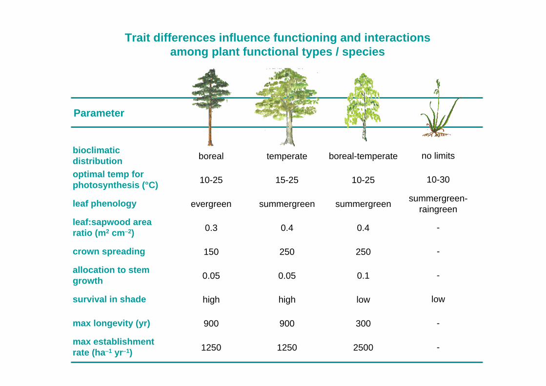
Parameter

max establishment rate (ha−1 yr−1)

max longevity (yr)

survival in shade

optimal temp for photosynthesis (°C)

bioclimatic distribution

allocation to stem growth

leaf:sapwood area ratio (m2 cm−2)

leaf phenology

crown spreading

boreal

10-25

evergreen

0.3

150

0.05

high

900

1250

temperate

15-25

summergreen

0.4

250

0.05

high

900

1250

boreal-temperate

10-25

summergreen

0.4

250

0.1

low

300

2500

no limits

10-30

summergreen-raingreen

-

-

-

low

-

-

Trait differences influence functioning and interactionsamong plant functional types / species

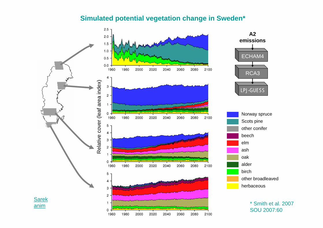
Simulated potential vegetation change in Sweden*

Rel

ativ

e co

ver (

leaf

are

a in

dex)

Norway spruceScots pineother coniferbeechelmashoakalderbirchother broadleavedherbaceous

* Smith et al. 2007SOU 2007:60

LPJ-GUESS

RCA3

A2emissions

ECHAM4

Sarekanim

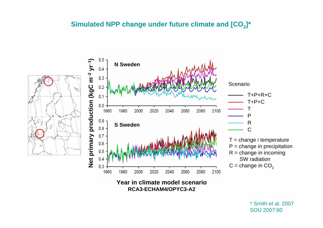
T+P+R+CT+P+CTP

T = change i temperatureP = change in precipitationR = change in incoming

SW radiationC = change in CO2

Scenario

RC

Year in climate model scenarioRCA3-ECHAM4/OPYC3-A2

Net

prim

ary

prod

uctio

n (k

gC m

−2yr

−1)

N Sweden

S Sweden

Simulated NPP change under future climate and [CO2]*

* Smith et al. 2007SOU 2007:60

–10 –5 –1 –0.5 –0.1 –0.05 0 0.05 0.1 0.5 1 5 10 kgC m–2

Change in terrestrial C stocks (2071-2100)–(1961-1990)

Vegetation C Soil C Vegetation+soil C

Simulated future changes in ecosystem C stocks(interactive regional climate-vegetation model)

LPJ-GUESS

RCA3

A1B emissions

ECHAM5

Simulated future NEE change depends onemissions scenario and climate model*

−0.10 −0.05 −0.01 0.100.050.01

NEE (kgC m−2 yr−1)

← sequestration emission →

Modern climate1961-1990

RCM / GCM / emissions scenario 2071-2100

LPJ-GUESS

RCM

emissionsscenario

AGCM

*Morales et al. 2007Global Change Biology 13: 108

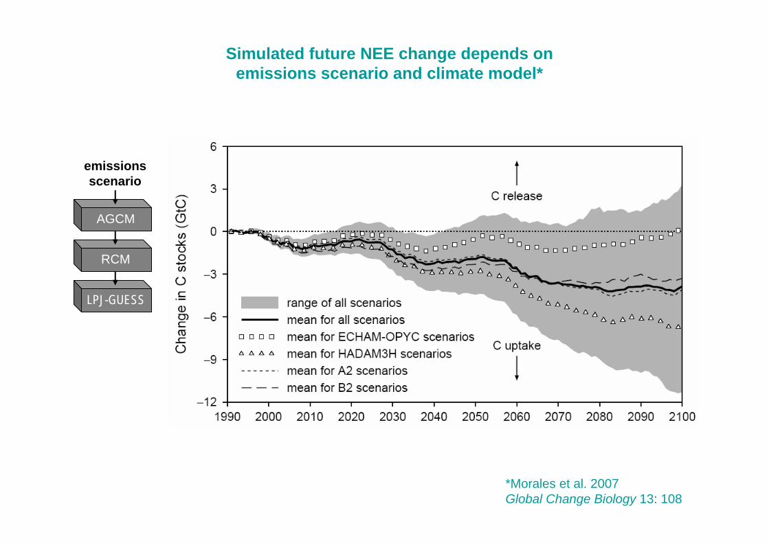
LPJ-GUESS

RCM

emissionsscenario

AGCM

Simulated future NEE change depends onemissions scenario and climate model*

*Morales et al. 2007Global Change Biology 13: 108

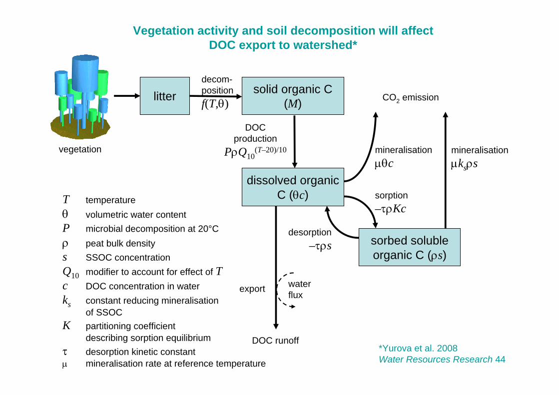
*Yurova et al. 2008Water Resources Research 44

Vegetation activity and soil decomposition will affectDOC export to watershed*

litter solid organic C(M)

decom-positionf(T,θ)

vegetation

DOCproduction

PρQ10(T–20)/10

dissolved organicC (θc)

sorbed solubleorganic C (ρs)

sorption–τρKc

desorption–τρs

mineralisationμksρs

mineralisationμθc

export

DOC runoff

CO2 emission

T temperatureθ volumetric water contentP microbial decomposition at 20°Cρ peat bulk densitys SSOC concentrationQ10 modifier to account for effect of Tc DOC concentration in waterks constant reducing mineralisation

of SSOCK partitioning coefficient

describing sorption equilibriumτ desorption kinetic constantμ mineralisation rate at reference temperature

waterflux

Modelled DOC production and exportfrom a Swedish boreal mire*

*Yurova et al. 2008Water Resources Research 44

modelled DOC storage

modelled DOC export

observed DOC export

modelled DOC production

modelled DOC export

ProductionExportgm−2

Exportmg l−1

Storagegm−2

Land use and land cover are the emergent outcomes ofbiophysical processes, human decision-making and interactions between them

Source: Global Land Project (GLP) Science Plan

*Pongratz et al. 2008Global Biogeochemical Cycles 22

Agricultural areas have expanded since pre-industrial times,typically replacing forest* ...

1700

1992

100 %63402516106.34.02.51.60

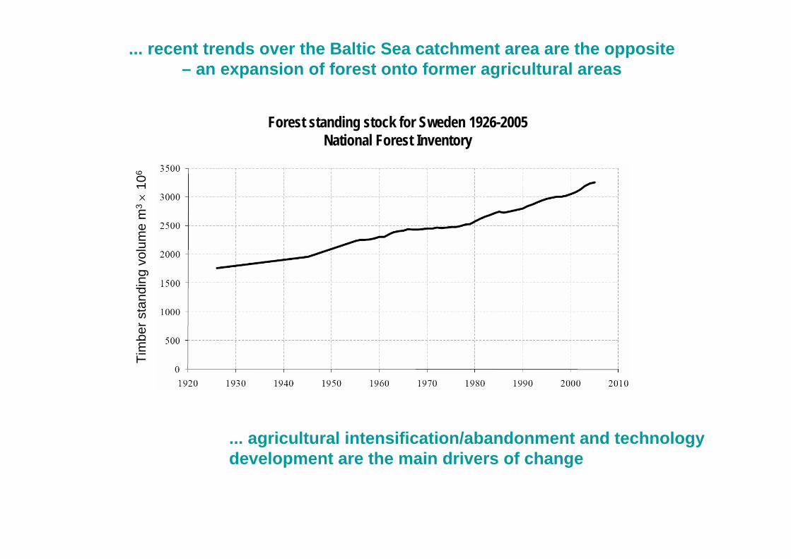
... recent trends over the Baltic Sea catchment area are the opposite– an expansion of forest onto former agricultural areas

Forest standing stock for Sweden 1926-2005National Forest Inventory

Tim

ber s

tand

ing

volu

me

m3×

106

... agricultural intensification/abandonment and technology development are the main drivers of change

*Rounsevell et al. 2006Agriculture, Ecosystems & Environment114: 57

Potential future land use changes derived by’automated interpretation’ of socio-economic scenario assumptions,

climate projections and ecosystem service changes*

• Three steps:→ Qualitative description of range and role of different scenario

assumptions for target region (e.g. populations, global and regional markets, ecosystem service supply, policy, technological change)

→ Quantitative assessment of area requirement of each land use type in response to changes in relevant drivers

→ Spatial allocation of resultant land use fractions across target area (based on land suitability, proximity to existing land use etc)

*I. Reginster & M. Rounsevell, EU FP6-ALARM

Main parameters* Sources

population UN population scenariogross domestic product (GDP) global econometric model GINFORS

demand for agricultural goods global econometric model GINFORSself-sufficiency index scenario interpretationclimate/physiology impact on crop yield ecosystem model LPJ-GUESS, simulated climatetechnological impact on crop yield scenario interpretationdemand for biofuels GINFORS, scenario interpretation

policy-driven changes in forest area policy analysis, scenario interpretationsurplus land change in other land use types

quantity, usage and type of protected area scenario interpretation

Urban

Agriculture

Forest

Protected

Potential future land use changes derived by’automated interpretation’ of socio-economic scenario assumptions,

climate projections and ecosystem service changes

−15

−10

−5

0

5

10

15

crop grass forest urban bioenergy protected surplus

−15

−10

−5

0

5

10

15

A2B1B2A1FI

PCM2CGCM2CSIRO2HadCM3

Land

-use

cov

er c

hang

e(%

of t

otal

land

are

a)Change in land use EU15+ 1990-2080

*Schröter et al. 2005.Science 310: 1333-1337

Projected land use changes for Europe under alternative scenarios*

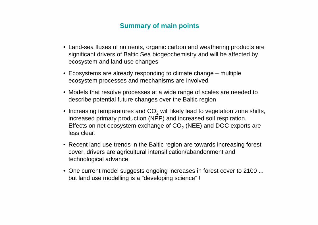
• Land-sea fluxes of nutrients, organic carbon and weathering products are significant drivers of Baltic Sea biogeochemistry and will be affected by ecosystem and land use changes

• Ecosystems are already responding to climate change – multiple ecosystem processes and mechanisms are involved

• Models that resolve processes at a wide range of scales are needed to describe potential future changes over the Baltic region

• Increasing temperatures and CO2 will likely lead to vegetation zone shifts, increased primary production (NPP) and increased soil respiration. Effects on net ecosystem exchange of CO2 (NEE) and DOC exports are less clear.

• Recent land use trends in the Baltic region are towards increasing forest cover, drivers are agricultural intensification/abandonment and technological advance.

• One current model suggests ongoing increases in forest cover to 2100 ... but land use modelling is a ”developing science” !

Summary of main points