land degradation and the australian agricultural industry · 2.1 state budgetary outlays benefiting...
TRANSCRIPT
LAND DEGRADATIONAND THE AUSTRALIAN
AGRICULTURALINDUSTRY
Paul Gretton
Umme Salma
STAFF INFORMATION PAPER
1996
INDUSTRYCOMMISSION
© Commonwealth of Australia 1996
ISBN
This work is copyright. Apart from any use as permitted under the Copyright Act 1968, thework may be reproduced in whole or in part for study or training purposes, subject to theinclusion of an acknowledgment of the source. Reproduction for commercial usage or salerequires prior written permission from the Australian Government Publishing Service.Requests and inquiries concerning reproduction and rights should be addressed to theManager, Commonwealth Information Services, AGPS, GPO Box 84, Canberra ACT 2601.
Enquiries
Paul GrettonIndustry CommissionPO Box 80BELCONNEN ACT 2616
Phone: (06) 240 3252Email: [email protected]
The views expressed in this paper do not necessarily reflect those ofthe Industry Commission.
Forming the Productivity Commission
The Federal Government, as part of its broader microeconomic reform agenda, is mergingthe Bureau of Industry Economics, the Economic Planning Advisory Commission and theIndustry Commission to form the Productivity Commission. The three agencies are now co-located in the Treasury portfolio and amalgamation has begun on an administrative basis.
While appropriate arrangements are being finalised, the work program of each of theagencies will continue. The relevant legislation will be introduced soon. This report has beenproduced by the Industry Commission.
iii
CONTENTS
Abbreviations vPreface vii
Overview ix
Part 1 Report
1 Introduction 12 Agriculture and the management of land 33 Sustainability and land degradation 194 Economic effects of land degradation in Australia 39
Part 2 Appendices
A Classification of agricultural land degradation in Australia A1B Classification of agricultural regions in New South Wales B1C The extent of land degradation in Australia C1D Conceptual model of land degradation, farm output and profits D1E Production equivalent of degradation, and costs and benefits of
amelioration E1F Estimates of the effects of land degradation in New South Wales F1
References
STAFF INFORMATION PAPER
iv
Boxes3.1 Pilot study using data on the biogeographic regionalisation 32
of New South Wales4.1 The Commission’s econometric model of New South Wales 50
agriculture
Tables2.1 State budgetary outlays benefiting agriculture by type of 13
support, 1990–912.2 Estimated agricultural sector environmental protection 15
expenditures by state, 1991–922.3 Grants and subsidies received by farm businesses by state, 16
1991–922.4 Expenditure on land care by broadacre farms and the dairy 17
industry, 1993–942.5 Main reasons for broadacre and dairy industry farms not
undertaking land 17care expenditure, 1993–94
4.1 Estimated responsiveness of current production and profit 51due to changing land degradation
Figures2.1 Farmers’ terms of trade, 1951–52 to 1993–94 42.2 Deployment of land for agricultural uses 62.3 Trends in average wheat yields since 1870 72.4 Contributions to average annual growth in real output by the 8
agriculture, forestry, fishing and hunting sector, 1974–75 to1993–94
2.5 Commonwealth budgetary outlays to industry, 1994–95 123.1 Economic-environmental input-output framework 234.1 Index of land degradation by type of degradation and 45
agricultural SLA in New South Wales, 1987–19884.2 Marginal net benefits from controlling dryland salinity with and 47
without commercial trees
LAND DEGRADATION AND THE AUSTRALIAN AGRICULTURAL INDUSTRY
v
ABBREVIATIONS
na not availablekg/ha kilograms per hectare.. nil or less than 0.50 small value rounded to zero in tablesAAGIS Australian Agricultural and Grazing Industries SurveyABARE Australian Bureau of Agricultural and Resource EconomicsABS Australian Bureau of StatisticsANCA Australian Nature Conservation AgencyAPEC Asia Pacific Economic CooperationBRS Bureau of Resource SciencesCSIRO Commonwealth Scientific and Industrial Research OrganisationELZ Extensive Landuse ZoneESD Ecologically Sustainable DevelopmentFAO Food and Agricultural OrganisationGIS Geographic Information System(s)IBRA Interim Biogeographic Regionalisation of AustraliaIC Industry CommissionILZ Intensive Landuse ZoneIMF International Monetary FundIUCN International Union for Conservation of Natural ResourcesNAFTA North Atlantic Free Trade AgreementNRIC National Resource Information CentreNRSCP National Reserve System Conservation PlanNSW New South WalesOECD Organisation for Economic Cooperation and DevelopmentR&D Research and DevelopmentRDC Rural research and development corporation/councilSCS Soil Conservation ServiceSLA Statistical Local AreaUN United NationsUNCED United Nations Conference on Environment and DevelopmentUNEP United Nations Environment ProgrammeUNESCO United nations Education, Science and Cultural OrganisationWWF World Wildlife Fund

vii
PREFACE
The Industry Commission has a statutory obligation to report on theperformance of Australian industry. Management of land for agricultural andpastoral purposes on a sustainable basis is essential for the ongoingdevelopment of that sector.
For development and environmental issues to be adequately considered, a broadframework needs to be adopted and necessary information of both an ecologicaland economic nature needs to be gathered and analysed.
As part of its reporting process, this staff paper has drawn together certaininformation and has used a pilot study of New South Wales agriculture as a startto the very substantial task of understanding the relationship betweenagricultural production and land degradation.
The Commission intends this discussion paper to bring together informationabout agriculture and land degradation from a wide range of sources and indoing so it is intended that it contributes to the development of a broad policyframework for a sustainable agricultural sector. The Commission seekscomments on the content of the paper, errors and ommissions.
The authors would like to acknowledge the assistance received from colleaguesin the preparation of the study. Outside the Commission, John Robertson of theDepartment of Statistics at the Australian National University provided atechnical review on the New South Wales pilot study (see Appendix F) andWarren Musgrave of the New South Wales Premier’s Department gave generalsupport. Numerous other people provided information and studies. Anyremaining errors are the responsibility of the authors.

ix
OVERVIEW
The management of land degradation and its effects on environmental qualityare important challenges. How the community responds to these challenges willaffect the well being of all Australians both now and into the future. There aremany causes of land degradation resulting from human activities, including theproduction of food and fibres by the agricultural sector.
This study explores the relationships between agricultural production,profitability and land degradation, and some of the broad issues that affect landmanagement. In particular, it discusses the concept of ecologically sustainabledevelopment, the link between bio-physical and economic processes,information on the extent of land degradation, and the costs and benefits ofdegradation and repair. An experimental analysis of New South Walesagriculture is provided using a state-wide model developed in the Commission.
The agricultural industry and management of land
The agricultural sector is constrained in its capacity to increase supply and toinfluence demand. The supply of land suitable for agricultural activities islimited and its availability for agriculture comes under pressure from alternativeuses. At the same time, the agricultural sector predominantly produces standardcommodities (often traded on world markets) with individual producers havingvirtually no control over the prices that they receive for their output, nor theprices paid for their off-farm inputs to production.
The agricultural sector has experienced a systematic decline in its terms of tradeover the last 40 years. To the extent that expectations about future prices havebeen based on the continuation of past trends alone, the incentives facingindividual farmers would seem to have favoured early exploitation of the landresource in order to take advantage of relatively higher prices. However, pastprice trends are only part of the picture. Innovation to lower the unit cost ofoutput, the expectation of a more favourable price outlook in the future, and theopportunity to vary farm outputs to take advantage of more profitable farmingoptions, improve the economic incentives for land holders to preserve landresources for future agricultural use.
In practice, productivity growth has steadily improved with support fromindustry and government sponsored research and development, and withexperience gained through farming Australian land. Over the last 20 years,agricultural sector growth has been sustained by more intensive use of existing
STAFF INFORMATION PAPER
x
farmland and by higher productivity. Opportunities for growth in agriculturaloutput will continue. The positive links between rural research, development,farmer experience and productivity indicate the potential for further growth inoutput from supply-side changes.
On the demand side, there are population, income and policy induced changesthat are likely to place upward pressure on the demand for Australianagricultural outputs in the longer term. These will come from increasing foodneeds in Australia and elsewhere (through exports) as populations increase andincomes rise. Australian agriculture is also likely to benefit as internationaltrade liberalisation is extended. Commission estimates suggest that Australianagricultural output could expand by 5 per cent with the implementation of theUruguay Round of trade negotiations and a further 12 per cent under the APECfree trade agenda.
Agricultural land use, along with other human activities, imposes pressures onthe environment as land resources are increasingly used in production andconsumption and as wastes are released. The management of those pressuresinvolves both public and private spending and effort to conserve theenvironment for future use. Information is now becoming available concerningthe level and purpose of environmental expenditure in Australia. ABS estimatesof public and private environmental expenditures in 1991–92 suggest a nation-wide total for that year of at least $5.2 billion. Of this total, soil conservationand land management activities of the public sector amounted to $198 million.A substantial part of this spending is directed at agricultural resourcemanagement and support services. Measured private sector environmentalspending by the agriculture sector amounted to $285 million, that is, about2 per cent of the value of agricultural production. The management of land toconserve resources, however, does not imply that land degradation will notoccur. Indeed some land degradation occurs naturally, that is, without humanuse or interferance.
Sustainability and land degradation
Available evidence suggests that land degradation in Australia is substantial.The forms of degradation vary widely and include: changing soil mineralisation,such as salinity and acidity; soil structure decline and erosion caused by waterand wind; and biological changes such as plant and animal invasion, tree declineand the clearance of native vegetation.
Several of the most prominent forms of degradation such as soil structuredecline and induced soil acidity are site specific and reversible. The initialeffects of these forms of degradation occurs at the individual farm level with
LAND DEGRADATION AND THE AUSTRALIAN AGRICULTURAL INDUSTRY
xi
few spillovers to adjacent properties and areas. Other forms of degradation suchas dryland and irrigation salinity relate to catchment or biogeographic regionsand can be classed as reversible, too. In other cases such as loss of top soil, andloss of native habitats, flora and fauna, the natural repair periods are so long thatfor practical purposes, damage arising from human activities could be deemedas permanent.
An important question for sustainability is: will the generation of currentincome lead to a permanent reduction in national productivity and will essentiallife support systems be threatened? If degradation is irreversible — or if it canonly be reversed at an uneconomic cost — those land uses dependent on theavailability of non-degraded land are not sustainable without technologicalchange.
Because the effects of degradation cannot always be confined to individualholdings, land degradation and its repair cannot be treated solely as a problemfor individual farmers. They may not see the full social costs of degradation andmay not be able to appropriate the full social benefits of conservation efforts.
Economic effects of land degradation
Land degradation involves reductions in the productivity of affected lands. Thereduction in productivity — estimated as the decline from value of productionobtainable with current land uses had there been no degradation — provides ameasure of the production equivalent of degradation. A recent PrimeMinisterial statement put the production equivalent of degradation at around6 per cent of agricultural production or around $1.5 billion (in 1994–95 values)each year.
Production equivalent measures, so defined, are static and are compiled usingrestrictive assumptions that ignore accumulated net benefits to the communityof past agricultural production and the productivity of farming activitiesoperating in localities where degradation occurs. In addition, productionequivalents do not take into account the fact that some degradation is likely tooccur as farming systems become more specialised and land productivity isimproved (eg irrigation farming and irrigation salinity) while other forms occuras unintended side effects of previous conservation efforts (eg improvedpastures and induced acidity). For these reasons, the production equivalentmeasure is not a true reflection of the current cost of degradation. Nevertheless,it does clearly indicate that the usefulness of some elements of the landscape issubstantially reduced by degradation.
Another approach to evaluating the impact of degradation on farming activity isto consider the costs of repairing or avoiding degradation and the benefits
STAFF INFORMATION PAPER
xii
available from conservation programs. Available cost-benefit studies indicatethat for irrigation and dryland salinity in some badly affected areas net benefitscould be obtained by public- and farm-based programs to repair the degradation,given plausible discount rates and project planning horizons. Nevertheless,using the same assumptions, the studies do not always imply that eliminating thedegradation is the most profitable course of action. Sometimes the highestreturns can be obtained by slowing the rate of spread rather than halting orreversing the degradation and sometimes even by allowing degradation toincrease. In addition, the costs of degradation can be substantially reduced bymoving in favour of farming activities that minimise the adverse effects on farmprofitability of the prevailing forms of degradation.
In other cases, the technology to repair degradation may be available, but onlysome agricultural activities generate the farm income to support conservationactivities. For example, induced soil acidity can normally be lowered, and theproductivity of the land increased, by the application of lime. This treatment iscostly to the farmer and the feasibility of conservation expenditure depends onsufficiently increased returns per hectare to justify the liming expense.
Available cost-benefit studies are concerned with particular products or regions.They possibly exclude farming options that may be more profitable givenprevailing discount rates and project planning horizons, but which areassociated with even higher levels of degradation.
To make a start towards establishing a comprehensive empirical analysis ofdegradation, the Commission developed a state-wide model of New SouthWales agriculture incorporating land degradation. The study focused on theeffects of four forms of degradation: irrigation salinity, dryland salinity, soilstructure decline, and induced soil acidity. The analysis represents a snapshot ofNew South Wales agriculture with the findings determined by prevailing levelsof degradation and current farming systems. The model implicitly takes accountof the opportunity costs to individual farmers of additional degradation. Withinits framework, farmers are treated as choosing between activities that yieldhigher production and degradation in the current period with lower productionin the future, and activities that yield lower production and degradation now toobtain higher production in the future.
The analysis tentatively indicates that there are incentives for individual farmersto move away from farming activities that induce higher levels of soil acidity orsoil structure decline (indeed, available evidence suggests that new techniquesare being adopted to ameliorate the effects of these forms of degradation). Theapparent driving force behind this result is that these forms of degradation affectwhole cultivated areas, reducing the productivity of the entire area. On theother hand, there appear to be positive incentives for farmers in New South
LAND DEGRADATION AND THE AUSTRALIAN AGRICULTURAL INDUSTRY
xiii
Wales to move towards activities associated with irrigation and dryland salinity.The driving force behind these results, is that these forms of degradationseverely affect individual locations in otherwise productive farming areas.Farmers are willing to sacrifice those locations as part of a generally productivefarming activity.
The constraining factor on the extension of farming systems subject to irrigationand dryland salinity may well be the availability of water for irrigation and ofland typically subject to dryland salinity, rather than the adverse effects of theseforms of degradation as such.
Because these results are based on a current snapshot of New South Wales, theydo not take into account the dynamic effects of technological change and othersources of productivity improvement. Technological change and better landmanagement may be able to improve farm productivity and profitability in allareas subject to degradation.
Summing up
The management of environmental expenditures and conservation effort is not astraightforward task. It is difficult even when measures of the usefulness ofland resources and degradation can be expressed in financial terms oragricultural sector outcomes as in the above studies. It is made more difficultwhen some of the outcomes are non-market, such as, the effects of farming onthe functioning of traditional ecological systems which are not easily factoredinto quantitative analyses. In assessments of the nature and role of governmentin agricultural land management as opposed to the role of individual farmers,there is a need to consider the property rights of farmers over land resourcessubject to degradation, and the trade-offs that occur between non-market landmanagement objectives and agricultural sector productivity and profitability.There is also a need to consider impediments faced by individual farmers toecologically sustainable agricultural land management imposed by governmentregulations, and other institutional arrangements.
With market-based outcomes, assessments of land degradation need to considerfarm productivity, production and income with prevailing levels of degradation,the likely prospects of alternative farming activities given expected prices andtechnological developments, the effect these activities are likely to have on thefuture condition of the land, and the costs and benefits of reclaiming degradedland. To provide a community-wide perspective of the social benefits of higherfarm productivity, it is also necessary to consider the external effects of thedegradation on other farmers and the community generally, alternative land
STAFF INFORMATION PAPER
xiv
uses, and the time horizon over which the costs and benefits should beevaluated.
The Commission’s modelling effort has made tentative steps towards anappraisal of agricultural land degradation and farm profitability. There is a needfor further research into the relationships between agricultural land degradation,farm productivity and profitability for the states and Australia. To supporteconomy-wide assessments that are firmly based on the current activities anddecisions of farmers in agricultural regions, there is also a need to improve theavailability of information on land degradation and the environment, anddevelop links between that information and data about farm activities anddecisions.

PART 1 REPORT

1
CHAPTER 1INTRODUCTION
Land degradation can occur for many reasons associated with human activities.This study focuses on land degradation related to agricultural production andprofitability. There are many causes of land degradation resulting from the useof land resources in agricultural production alone. Fundamental factorsdetermining the nature and extent of degradation are the bio-physicalcharacteristics of the land, economic imperatives and awareness of the fullimpact of farming practices.
Managing agriculture within the philosophy established by the National Strategyfor Ecologically Sustainable Development, requires knowledge of the landdegradation process, the current state of land resources and establishing a wayto relate possible future degradation to management decisions.
This information paper draws together certain information and analyses as atentative step towards understanding some of the issues faced by the agriculturalsector in its management of land. It is structured as follows. Chapter 2provides an overview of the agricultural sector and broad issues that affect landmanagement. Chapter 3 discusses the concept of ecologically sustainabledevelopment, the definition of land degradation and the link between bio-physical and economic processes of land degradation. In Chapter 4, informationabout the extent of degradation, the costs and benefits of amelioration and anexperimental state-wide model for New South Wales agriculture incorporatingland degradation are provided and discussed.
The scope of the study has been limited. For example, it has not examined indetail levels of government support and assistance to the agricultural industryand how this has affected or could affect land use and degradation. The studyalso has not examined the many institutional arrangements that have beenestablished for managing the land (such as catchment plans). Such matters andothers will affect the level and incidence of degradation and the sustainability ofagriculture in the Australian economy.

3
CHAPTER 2AGRICULTURE AND THE MANAGEMENT OFLAND
2.1 Introduction
Land if left to degrade with agricultural use, would inevitably becomeunproductive for that use. The effect of declining productivity of existingagricultural land is pressure to change land management practices in order toreverse this trend where feasible, or to replace degraded land by clearing andbringing into production previously unfarmed land.
Each individual producer can have a significant effect on the use and conditionof their land but each has little or no effect on the prices of their products. Theagricultural sector predominantly produces standard commodities (often tradedon world markets) with individual producers having virtually no control overthe prices that they receive for their output nor the prices paid for their off-farminputs to production.
This chapter presents a general picture of the broad economic environment inwhich the agricultural sector operates. This provides a backdrop against whichspecific information about land degradation can be developed. The chapterlooks at the terms of trade of the agricultural sector, contributions to growth inagriculture and the links between rural research and development (R&D) andindustry growth, Commonwealth budgetary outlays to industry, andenvironmental spending by government and industry.
2.2 Farmers’ terms of trade
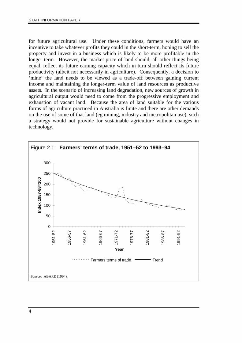
One of the most fundamental factors governing the economic environment inwhich farmers operate is the prices that they receive for their outputs relative tothe prices that they pay for their farm inputs — that is, the farmers’ terms oftrade. For the Australian rural industry, the terms of trade have declined overthe past 40 years at an average annual rate of 2 per cent per annum around aseries of erratic year to year changes (see Figure 2.1).
Without innovation to lower the unit cost of output or the expectation ofincreasing prices, other things being equal, the trend in relative prices wouldhave provided a poor economic incentive for land holders to preserve the land
STAFF INFORMATION PAPER
4
for future agricultural use. Under these conditions, farmers would have anincentive to take whatever profits they could in the short-term, hoping to sell theproperty and invest in a business which is likely to be more profitable in thelonger term. However, the market price of land should, all other things beingequal, reflect its future earning capacity which in turn should reflect its futureproductivity (albeit not necessarily in agriculture). Consequently, a decision to‘mine’ the land needs to be viewed as a trade-off between gaining currentincome and maintaining the longer-term value of land resources as productiveassets. In the scenario of increasing land degradation, new sources of growth inagricultural output would need to come from the progressive employment andexhaustion of vacant land. Because the area of land suitable for the variousforms of agriculture practiced in Australia is finite and there are other demandson the use of some of that land (eg mining, industry and metropolitan use), sucha strategy would not provide for sustainable agriculture without changes intechnology.
Figure 2.1: Farmers’ terms of trade, 1951–52 to 1993–94
Year
Ind
ex 1
987-
88=1
00
0
50
100
150
200
250
300
1951
-52
1956
-57
1961
-62
1966
-67
1971
-72
1976
-77
1981
-82
1986
-87
1991
-92
Farmers terms of trade Trend
Source: ABARE (1994).
2 AGRICULTURE AND THE MANAGEMENT OF LAND
5
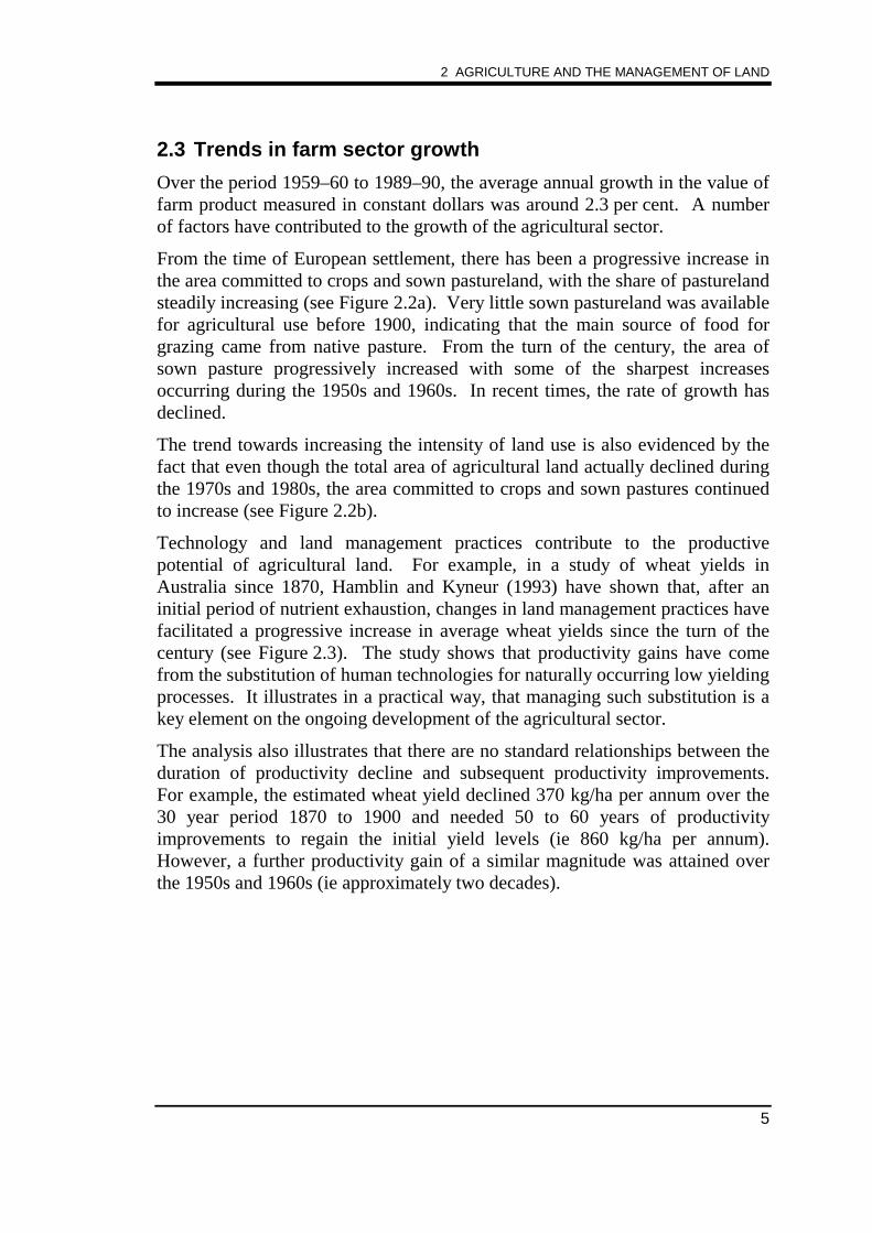
2.3 Trends in farm sector growth
Over the period 1959–60 to 1989–90, the average annual growth in the value offarm product measured in constant dollars was around 2.3 per cent. A numberof factors have contributed to the growth of the agricultural sector.
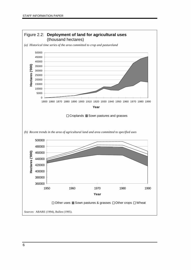
From the time of European settlement, there has been a progressive increase inthe area committed to crops and sown pastureland, with the share of pasturelandsteadily increasing (see Figure 2.2a). Very little sown pastureland was availablefor agricultural use before 1900, indicating that the main source of food forgrazing came from native pasture. From the turn of the century, the area ofsown pasture progressively increased with some of the sharpest increasesoccurring during the 1950s and 1960s. In recent times, the rate of growth hasdeclined.
The trend towards increasing the intensity of land use is also evidenced by thefact that even though the total area of agricultural land actually declined duringthe 1970s and 1980s, the area committed to crops and sown pastures continuedto increase (see Figure 2.2b).
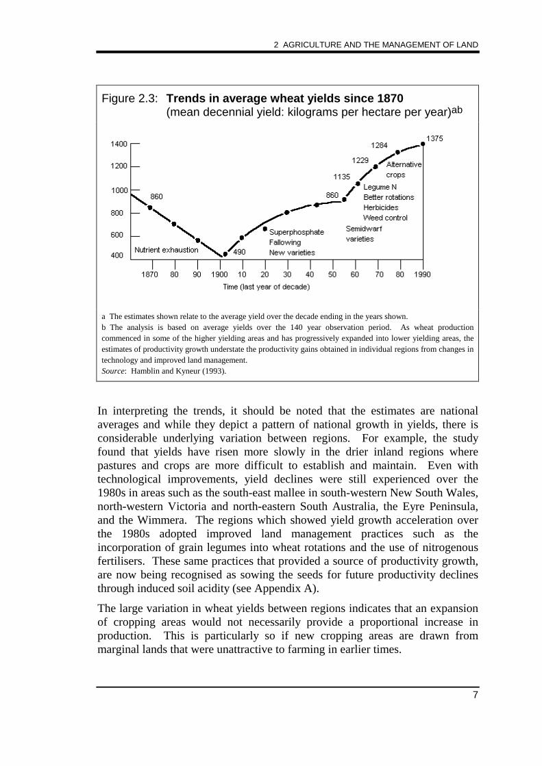
Technology and land management practices contribute to the productivepotential of agricultural land. For example, in a study of wheat yields inAustralia since 1870, Hamblin and Kyneur (1993) have shown that, after aninitial period of nutrient exhaustion, changes in land management practices havefacilitated a progressive increase in average wheat yields since the turn of thecentury (see Figure 2.3). The study shows that productivity gains have comefrom the substitution of human technologies for naturally occurring low yieldingprocesses. It illustrates in a practical way, that managing such substitution is akey element on the ongoing development of the agricultural sector.
The analysis also illustrates that there are no standard relationships between theduration of productivity decline and subsequent productivity improvements.For example, the estimated wheat yield declined 370 kg/ha per annum over the30 year period 1870 to 1900 and needed 50 to 60 years of productivityimprovements to regain the initial yield levels (ie 860 kg/ha per annum).However, a further productivity gain of a similar magnitude was attained overthe 1950s and 1960s (ie approximately two decades).
STAFF INFORMATION PAPER
6
Figure 2.2: Deployment of land for agricultural uses(thousand hectares)
(a) Historical time series of the area committed to crop and pastureland
0
5000
10000
15000
20000
25000
30000
35000
40000
45000
50000
1800 1860 1870 1880 1890 1900 1910 1920 1930 1940 1950 1960 1970 1980 1990
Year
Hec
tare
s (’0
00)
Croplands Sown pastures and grasses
(b) Recent trends in the area of agricultural land and area committed to specified uses
360000
380000
400000
420000
440000
460000
480000
500000
1950 1960 1970 1980 1990
Year
Hec
tare
s (’0
00)
Other uses Sown pastures & grasses Other crops Wheat
Sources: ABARE (1994), Bullen (1995).
2 AGRICULTURE AND THE MANAGEMENT OF LAND
7
Figure 2.3: Trends in average wheat yields since 1870(mean decennial yield: kilograms per hectare per year)ab
a The estimates shown relate to the average yield over the decade ending in the years shown.b The analysis is based on average yields over the 140 year observation period. As wheat productioncommenced in some of the higher yielding areas and has progressively expanded into lower yielding areas, theestimates of productivity growth understate the productivity gains obtained in individual regions from changes intechnology and improved land management.Source: Hamblin and Kyneur (1993).
In interpreting the trends, it should be noted that the estimates are nationalaverages and while they depict a pattern of national growth in yields, there isconsiderable underlying variation between regions. For example, the studyfound that yields have risen more slowly in the drier inland regions wherepastures and crops are more difficult to establish and maintain. Even withtechnological improvements, yield declines were still experienced over the1980s in areas such as the south-east mallee in south-western New South Wales,north-western Victoria and north-eastern South Australia, the Eyre Peninsula,and the Wimmera. The regions which showed yield growth acceleration overthe 1980s adopted improved land management practices such as theincorporation of grain legumes into wheat rotations and the use of nitrogenousfertilisers. These same practices that provided a source of productivity growth,are now being recognised as sowing the seeds for future productivity declinesthrough induced soil acidity (see Appendix A).
The large variation in wheat yields between regions indicates that an expansionof cropping areas would not necessarily provide a proportional increase inproduction. This is particularly so if new cropping areas are drawn frommarginal lands that were unattractive to farming in earlier times.
STAFF INFORMATION PAPER
8
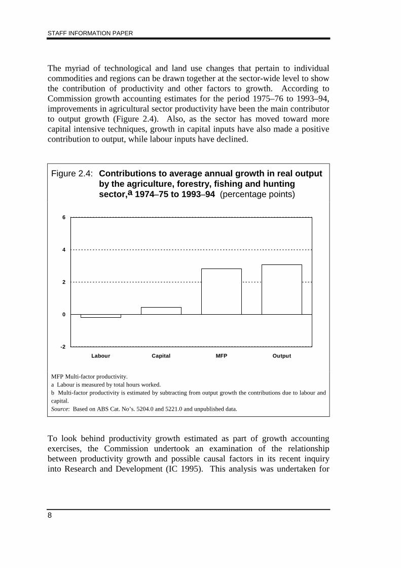
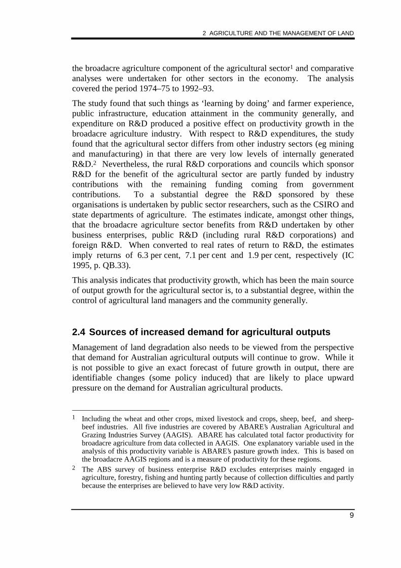
The myriad of technological and land use changes that pertain to individualcommodities and regions can be drawn together at the sector-wide level to showthe contribution of productivity and other factors to growth. According toCommission growth accounting estimates for the period 1975–76 to 1993–94,improvements in agricultural sector productivity have been the main contributorto output growth (Figure 2.4). Also, as the sector has moved toward morecapital intensive techniques, growth in capital inputs have also made a positivecontribution to output, while labour inputs have declined.
Figure 2.4: Contributions to average annual growth in real outputby the agriculture, forestry, fishing and huntingsector,a 1974–75 to 1993–94 (percentage points)
-2
0
2
4
6
Labour Capital MFP Output
MFP Multi-factor productivity.a Labour is measured by total hours worked.b Multi-factor productivity is estimated by subtracting from output growth the contributions due to labour andcapital.Source: Based on ABS Cat. No’s. 5204.0 and 5221.0 and unpublished data.
To look behind productivity growth estimated as part of growth accountingexercises, the Commission undertook an examination of the relationshipbetween productivity growth and possible causal factors in its recent inquiryinto Research and Development (IC 1995). This analysis was undertaken for
2 AGRICULTURE AND THE MANAGEMENT OF LAND
9
the broadacre agriculture component of the agricultural sector1 and comparativeanalyses were undertaken for other sectors in the economy. The analysiscovered the period 1974–75 to 1992–93.
The study found that such things as ‘learning by doing’ and farmer experience,public infrastructure, education attainment in the community generally, andexpenditure on R&D produced a positive effect on productivity growth in thebroadacre agriculture industry. With respect to R&D expenditures, the studyfound that the agricultural sector differs from other industry sectors (eg miningand manufacturing) in that there are very low levels of internally generatedR&D.2 Nevertheless, the rural R&D corporations and councils which sponsorR&D for the benefit of the agricultural sector are partly funded by industrycontributions with the remaining funding coming from governmentcontributions. To a substantial degree the R&D sponsored by theseorganisations is undertaken by public sector researchers, such as the CSIRO andstate departments of agriculture. The estimates indicate, amongst other things,that the broadacre agriculture sector benefits from R&D undertaken by otherbusiness enterprises, public R&D (including rural R&D corporations) andforeign R&D. When converted to real rates of return to R&D, the estimatesimply returns of 6.3 per cent, 7.1 per cent and 1.9 per cent, respectively (IC1995, p. QB.33).
This analysis indicates that productivity growth, which has been the main sourceof output growth for the agricultural sector is, to a substantial degree, within thecontrol of agricultural land managers and the community generally.
2.4 Sources of increased demand for agricultural outputs
Management of land degradation also needs to be viewed from the perspectivethat demand for Australian agricultural outputs will continue to grow. While itis not possible to give an exact forecast of future growth in output, there areidentifiable changes (some policy induced) that are likely to place upwardpressure on the demand for Australian agricultural products.
1 Including the wheat and other crops, mixed livestock and crops, sheep, beef, and sheep-
beef industries. All five industries are covered by ABARE’s Australian Agricultural andGrazing Industries Survey (AAGIS). ABARE has calculated total factor productivity forbroadacre agriculture from data collected in AAGIS. One explanatory variable used in theanalysis of this productivity variable is ABARE’s pasture growth index. This is based onthe broadacre AAGIS regions and is a measure of productivity for these regions.
2 The ABS survey of business enterprise R&D excludes enterprises mainly engaged inagriculture, forestry, fishing and hunting partly because of collection difficulties and partlybecause the enterprises are believed to have very low R&D activity.
STAFF INFORMATION PAPER
10
All things being equal, there are likely increases in demand due to the foodneeds of Australian and foreign residents (through exports) as the population ofAustralia and other countries increases and as incomes grow world-wide.
Australian agricultural producers are also likely to benefit as international tradeliberalisation is extended to this sector. It is generally accepted that tradeliberalisation would tend to raise the average world prices of agricultural andfood products, as export and production subsidies afforded these products inmany countries are scaled down or removed. Australia, with an export orientedand relatively lowly assisted agricultural and food processing sector, wouldexpect to see an increase in demand from these international developments. Forexample:
• simulations of the effects on Australia’s economy of implementation of theUruguay Round suggest agricultural output could expand by 5.5 per centand exports by 7.6 per cent (IC 1994). Subsequent annual growth inagricultural output and export would then continue from the post-Uruguayround output and production bases; and
• simulation of the impact of the implementation of Asia Pacific EconomicCooperation free trade commitments (under the principle ofcomprehensiveness confirmed at the Osaka 1995 meeting of APECmembers) suggests that Australian agricultural output could expand12.3 per cent against a benchmark established after the impact of theUruguay Round and the North Atlantic Free Trade Agreement(Dee et al. 1996). The analysis showed that the liberalisation ofagriculture would be the main force behind gains from the liberalisation ofmerchandise trade, contributing 60 per cent of total gains worldwide.
The Uruguay Round was completed in December 1993 and the agreedliberalisation processes are to be implemented by developed countries by 2001.Currently, liberalisation under the auspices of APEC agreements is to beimplemented by 2010 for developed countries and 2020 for developingcountries. The simulated changes in output are longer-run changes that wouldoccur progressively from the time of policy implementation.
Thus, the management of agricultural land in Australia will be undertaken forthe foreseeable future in an environment of increasing demands for agriculturaloutputs from the Australian industry.
2 AGRICULTURE AND THE MANAGEMENT OF LAND
11
2.5 Government expenditures on agriculture and agriculturalland management
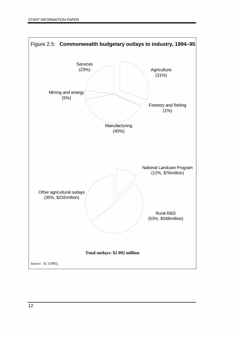
The operation and growth of the agricultural industry is supported by asubstantial level of government involvement. The agricultural sector receivedabout 31 per cent of Commonwealth Government outlays to industry in 1994–95 (ie around $650 million) (see Figure 2.5). Of the total support foragriculture, 12 per cent ($76 million) was allocated directly to the NationalLand Care Program. More than half of the expenditure was allocated to ruralR&D ($348 million) and is managed mainly through grants awarded through therural R&D corporations and direct funding to the Commonwealth Scientific andIndustrial Research Organisation.
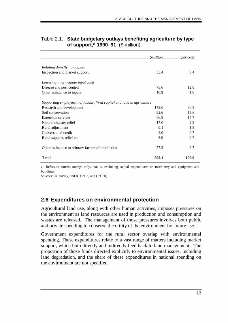
A Commission survey has also estimated that state expenditure benefiting therural sector would be at least $592 million (see 1990–91 estimate, Table 2.1).Around 16 per cent of these expenditures were committed to soil conservationservices, with 30 per cent going to research and development and a further13 per cent to disease and pest control. A comparison with an earlier 1981–82survey shows that expenditures nominated as benefiting soil conservationincreased from 5 per cent to 16 per cent of total expenditures (IC 1993). Overthe same period, total expenditures increased from $355 million to $592 million.The share of disease and pest control remained relatively stable while the shareof general research and extension services declined (from 36 per cent to30 per cent, and 23 per cent to 14 per cent, respectively). Because thecomposition of the general research and extension service categories is notdefined, the relative importance of soil conservation related work included inthose categories in the earlier survey but not in the latter is not evident. Thegrowth in relative importance of soil conservation services could thereforerepresent a combination of increased expenditures on those activities and areclassification of some activities from general categories. In either case, thereported growth of soil conservation expenditures indicates a heightened policyemphasis on it.
STAFF INFORMATION PAPER
12
Figure 2.5: Commonwealth budgetary outlays to industry, 1994–95
Agriculture(31%)
Forestry and fishing(1%)
Manufacturing(40%)
Mining and energy(5%)
Services(23%)
National Landcare Program(12%, $76million)
Rural R&D(53%, $348million)
Other agricultural outlays(35%, $232million)
Total outlays: $2 092 million
Source: IC (1995).
2 AGRICULTURE AND THE MANAGEMENT OF LAND
13
Table 2.1: State budgetary outlays benefiting agriculture by typeof support,a 1990–91 ($ million)
$million per cent
Relating directly to outputsInspection and market support 55.4 9.4
Lowering intermediate input costsDisease and pest control 75.6 12.8Other assistance to inputs 10.9 1.8
Supporting employment of labour, fixed capital and land in agricultureResearch and development 179.6 30.3Soil conservation 92.6 15.6Extension services 86.8 14.7Natural disaster relief 17.0 2.9Rural adjustment 9.1 1.5Concessional credit 4.0 0.7Rural support, relief etc 3.9 0.7
Other assistance to primary factors of production 57.3 9.7
Total 592.1 100.0
a Refers to current outlays only, that is, excluding capital expenditures on machinery and equipment andbuildings.Sources: IC survey, and IC (1993) and (1995b).
2.6 Expenditures on environmental protection
Agricultural land use, along with other human activities, imposes pressures onthe environment as land resources are used in production and consumption andwastes are released. The management of those pressures involves both publicand private spending to conserve the utility of the environment for future use.
Government expenditures for the rural sector overlap with environmentalspending. These expenditures relate to a vast range of matters including marketsupport, which both directly and indirectly feed back to land management. Theproportion of those funds directed explicitly to environmental issues, includingland degradation, and the share of these expenditures in national spending onthe environment are not specified.
STAFF INFORMATION PAPER
14
Nevertheless, some information on environmental expenditures by the publicand private sectors is provided in a recently published nation-wide study ofenvironmental expenditures (ABS 1995b). In addition, ABARE conducted asurvey of farm land care expenditure for 1993–94. The ABS collectionprovides a nation-wide focus on environmental spending and the ABAREsurvey provides a farm focus.
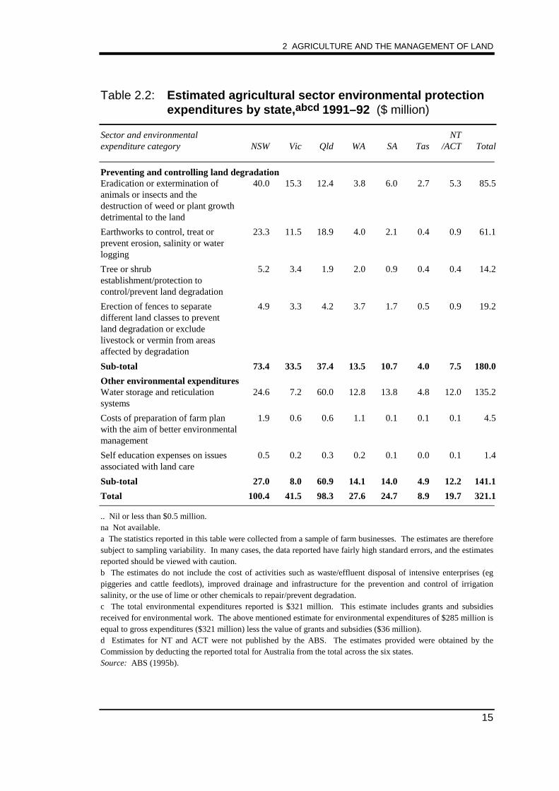
The ABS has estimated that the national level of environmental expenditures in1991–92 was around $5 153 million comprising $2 853 million in publicspending and $2 300 million in private sector industry expenditures. Of thetotal, about 4 per cent ($198 million) was allocated to soil conservation and landmanagement, while a further 5.5 per cent ($285 million) was environmentalexpenditures by farming enterprises. The industry expenditures are net ofgovernment grants and subsidies defined in the study to be concerned withenvironmental protection.
Net environmental protection expenditures by the agriculture sector comprise$321 million in industry spending less $36 million in grants and subsidies. Theindustry outlays of $321 million amount to nearly 2 per cent of the local valueof agricultural production ($18 billion in 1991–92). The scope ofenvironmental expenditures, as estimated, go well beyond measures that areeasily recognisable as anti-degradation activities. The most important item ofexpenditure relates to water storage and reticulation expenditures with around60 per cent of the total expenditure in this category coming from New SouthWales and Queensland (see Table 2.2). The second most important categoryrelates to the extermination of pests and insects. Only in Queensland is thisranking replaced by expenditures on earthworks to control, treat or preventerosion.
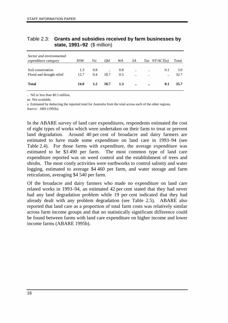
The estimated grants and subsidies are nearly totally comprised of flood anddrought relief (see Table 2.3). These expenditures are essentially short term innature varying from year to year according to climatic conditions and the currentrequirements for industry relief, rather than the longer-term condition ofagricultural land and sustainable agricultural enterprise. Only a small part of thegrant support relates to soil conservation.
2 AGRICULTURE AND THE MANAGEMENT OF LAND
15
Table 2.2: Estimated agricultural sector environmental protectionexpenditures by state,abcd 1991–92 ($ million)
Sector and environmentalexpenditure category NSW Vic Qld WA SA Tas
NT/ACT Total
Preventing and controlling land degradationEradication or extermination ofanimals or insects and thedestruction of weed or plant growthdetrimental to the land
40.0 15.3 12.4 3.8 6.0 2.7 5.3 85.5
Earthworks to control, treat orprevent erosion, salinity or waterlogging
23.3 11.5 18.9 4.0 2.1 0.4 0.9 61.1
Tree or shrubestablishment/protection tocontrol/prevent land degradation
5.2 3.4 1.9 2.0 0.9 0.4 0.4 14.2
Erection of fences to separatedifferent land classes to preventland degradation or excludelivestock or vermin from areasaffected by degradation
4.9 3.3 4.2 3.7 1.7 0.5 0.9 19.2
Sub-total 73.4 33.5 37.4 13.5 10.7 4.0 7.5 180.0
Other environmental expendituresWater storage and reticulationsystems
24.6 7.2 60.0 12.8 13.8 4.8 12.0 135.2
Costs of preparation of farm planwith the aim of better environmentalmanagement
1.9 0.6 0.6 1.1 0.1 0.1 0.1 4.5
Self education expenses on issuesassociated with land care
0.5 0.2 0.3 0.2 0.1 0.0 0.1 1.4
Sub-total 27.0 8.0 60.9 14.1 14.0 4.9 12.2 141.1
Total 100.4 41.5 98.3 27.6 24.7 8.9 19.7 321.1
.. Nil or less than $0.5 million.na Not available.a The statistics reported in this table were collected from a sample of farm businesses. The estimates are thereforesubject to sampling variability. In many cases, the data reported have fairly high standard errors, and the estimatesreported should be viewed with caution.b The estimates do not include the cost of activities such as waste/effluent disposal of intensive enterprises (egpiggeries and cattle feedlots), improved drainage and infrastructure for the prevention and control of irrigationsalinity, or the use of lime or other chemicals to repair/prevent degradation.c The total environmental expenditures reported is $321 million. This estimate includes grants and subsidiesreceived for environmental work. The above mentioned estimate for environmental expenditures of $285 million isequal to gross expenditures ($321 million) less the value of grants and subsidies ($36 million).d Estimates for NT and ACT were not published by the ABS. The estimates provided were obtained by theCommission by deducting the reported total for Australia from the total across the six states.Source: ABS (1995b).
STAFF INFORMATION PAPER
16
Table 2.3: Grants and subsidies received by farm businesses bystate, 1991–92 ($ million)
Sector and environmental expenditure category NSW Vic Qld WA SA Tas NT/ACT(a) Total
Soil conservation 1.3 0.8 .. 0.8 .. .. 0.1 3.0Flood and drought relief 12.7 0.4 18.7 0.5 .. .. .. 32.7
Total 14.0 1.2 18.7 1.3 .. .. 0.1 35.7
.. Nil or less than $0.5 million.na Not available.a Estimated by deducting the reported total for Australia from the total across each of the other regions.Source: ABS (1995b).
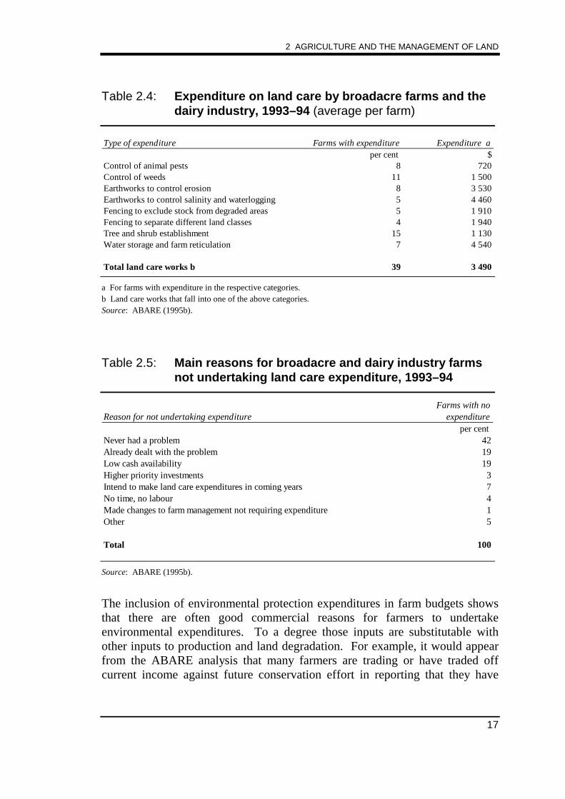
In the ABARE survey of land care expenditures, respondents estimated the costof eight types of works which were undertaken on their farm to treat or preventland degradation. Around 40 per cent of broadacre and dairy farmers areestimated to have made some expenditure on land care in 1993–94 (seeTable 2.4). For those farms with expenditure, the average expenditure wasestimated to be $3 490 per farm. The most common type of land careexpenditure reported was on weed control and the establishment of trees andshrubs. The most costly activities were earthworks to control salinity and waterlogging, estimated to average $4 460 per farm, and water storage and farmreticulation, averaging $4 540 per farm.
Of the broadacre and dairy farmers who made no expenditure on land carerelated works in 1993–94, an estimated 42 per cent stated that they had neverhad any land degradation problem while 19 per cent indicated that they hadalready dealt with any problem degradation (see Table 2.5). ABARE alsoreported that land care as a proportion of total farm costs was relatively similaracross farm income groups and that no statistically significant difference couldbe found between farms with land care expenditure on higher income and lowerincome farms (ABARE 1995b).
2 AGRICULTURE AND THE MANAGEMENT OF LAND
17
Table 2.4: Expenditure on land care by broadacre farms and thedairy industry, 1993–94 (average per farm)
Type of expenditure Farms with expenditure Expenditure aper cent $
Control of animal pests 8 720Control of weeds 11 1 500Earthworks to control erosion 8 3 530Earthworks to control salinity and waterlogging 5 4 460Fencing to exclude stock from degraded areas 5 1 910Fencing to separate different land classes 4 1 940Tree and shrub establishment 15 1 130Water storage and farm reticulation 7 4 540
Total land care works b 39 3 490
a For farms with expenditure in the respective categories.b Land care works that fall into one of the above categories.Source: ABARE (1995b).
Table 2.5: Main reasons for broadacre and dairy industry farmsnot undertaking land care expenditure, 1993–94
Reason for not undertaking expenditureFarms with no
expenditureper cent
Never had a problem 42Already dealt with the problem 19Low cash availability 19Higher priority investments 3Intend to make land care expenditures in coming years 7No time, no labour 4Made changes to farm management not requiring expenditure 1Other 5
Total 100
Source: ABARE (1995b).
The inclusion of environmental protection expenditures in farm budgets showsthat there are often good commercial reasons for farmers to undertakeenvironmental expenditures. To a degree those inputs are substitutable withother inputs to production and land degradation. For example, it would appearfrom the ABARE analysis that many farmers are trading or have traded offcurrent income against future conservation effort in reporting that they have
STAFF INFORMATION PAPER
18
either dealt with the problem (10 per cent of respondents) or plan to undertakeland care works at some future time (7 per cent of respondents).
The analysis indicates that there are trade offs being made by farmers withrespect to environmental expenditures in their total farm operation. Importantquestions for sustainable agriculture may concern the relationship between theexpenditure trade offs being made by farmers, farm profitability and longer-term sustainability. Also of concern would be impediments to sustainable landmanagement faced by individual farmers and imposed by governmentregulations and other institutional arrangements.
2.7 Conclusion
Improvements in productivity have provided one source of growth in theagricultural sector over the longer-term, with output of the farm sectorincreasing despite a longer term decline in the sector’s terms of trade.Productivity growth has also entailed more intensive use of farmlands.
Government and private environmental expenditure is undertaken in order tosupport the capacity of land to meet future agricultural and environmental uses.Such expenditure is part of a much larger national spending on environmentalactivities.
Environmental expenditures are, explicitly or implicitly, intended to sustainsome level of activity given the nature and capacity of the environment. To beeconomically and socially justified, those expenditures need to be accompaniedby net benefits to the community. The next chapter considers sustainableagriculture and the links between the agricultural sector and the environment.
19
CHAPTER 3SUSTAINABILITY AND LAND DEGRADATION
3.1 Introduction
This chapter discusses some of the major concepts that are necessary for anunderstanding of sustainability and land degradation. Sections 3.2 and 3.3outline an environmental-economic framework, and concepts and definitionsthat underlie a consideration of land degradation. Section 3.4 examines landdegradation in the context of ecologically sustainable development whileSection 3.5 discusses some of the driving forces behind the incidence of landdegradation. Section 3.6 considers whether land degradation is a private orsocial problem and Section 3.7 provides a conclusion to the chapter.
3.2 Environmental-economic framework
Introduction
Economic development involves, amongst other things, use of the naturalenvironment. The development of the agricultural sector has progressivelyinvolved more intensive use of land resources for cropping and grazing, andwith this, greater control and pressure on local habitats leading to environmentalchange. The development of the agricultural sector (along with other sectors ofthe economy), therefore, has involved adaptation to a changing environment.
The overall interaction between the production and consumption systems ofhumans and the environment can be conveniently summarised through asimplified presentation of the economy and the environment. This presentationcan then be used to produce a more systematic framework for linking theeconomy and the environment.
Economic activity is normally associated with the production of goods andservices using materials, labour and capital inputs and the consumption of thosecommodities. Production can be thought of as being undertaken by firms (orenterprises) and consumption by households who are also suppliers of labour.Government also enters the economic system as a producer of goods andservices and employer of labour and capital. The value of economic activity isnormally enumerated in monetary terms.
STAFF INFORMATION PAPER
20
Economic problems that involve the dimension of time can be captured bydiscounting, which is a procedure for finding the present value of a futurestream of benefits and costs. The rate at which benefits and costs are convertedto present values is the discount rate.
Discounting
Discount rates are usually positive for two underlying reasons. First, peoplegenerally discount the future because they prefer benefits sooner rather thanlater; and, secondly, if resources are diverted for investment, rather thanconsumption, those resources will be able to yield a higher level of consumptionin a future period.
Discount rates are used to capture both private and social time preferences.Private discount rates refer to the discount rate an individual would use whendeciding whether an investment would be worthwhile. It is the rate of return theindividual would have to receive to make that person willing to trade offconsumption now against consumption in the future — resources not used todaywould be an investment in the future. They indicate the opportunity cost ofcapital for the individual. Private discount rates are applicable in financialanalyses which are undertaken to assess whether an investment is profitable forthe individual undertaking it.
The social discount rate should reflect society’s valuation of the future and thetrade off society makes between consumption now and consumption in thefuture (ie social time preferences). It also represents the social opportunity costof capital funds in the economy as a whole.3 In a social discounting framework,public and private decisions would be appraised on a consistent basis that isconcerned with social welfare. Social discount rates are relevant to economicanalysis which is concerned with whether or not particular projects or policieswill improve community welfare. Other things being equal, the higher thesocial discount rate the greater the emphasis on resource use and investmentsthat provide income after short gestation periods. Benefits from resource use by
3 The social opportunity cost of capital and society’s valuation of the future, that is, the
marginal rate of time preference, are two sides of the same thing. The opportunity cost ofcapital represents the demand side for capital funds while the marginal rate of timepreference represents the supply side. In a perfectly competitive capital market, theequilibrium would occur in the capital market when the demand for capital funds exhaustssupply. The equilibrium social discount rate would be the rate that applied when supplyand demand are in equilibrium. However, capital markets are not always perfectlycompetitive and there are a number of possible approaches to estimating social discountrates. For further discussion of these issues in a cost benefit framework see Perkins(1994).
3 SUSTAINABILITY AND LAND DEGRADATION
21
future generations (or projects with long gestation periods) would be heavilydiscounted.
Social discounting requires that the social costs and benefits of private projects,rather than the financial outlays and receipts, be considered in the social (oreconomic) appraisal of projects. Social analysis therefore differs from privateanalysis in that private analysis does not take into account the external effectswhich are conferred on society but not on the private enterprise making thedecisions (such as down-stream pollution and spillover benefits to others of on-farm research and development). Even if those factors were included in theprivate appraisal of projects, the social discount rate would differ from theprivate discount rate for reasons such as imperfections in the capital market(which drive a wedge between borrowing and lending rates), the effects of taxes(which are costs to the individual, but transfers to society as a whole), and risk(which takes account of differences in riskiness of private and public sectorprojects).
The application of discounting depends on economic and environmental flowsbeing valued in monetary terms. This is not the case when the benefits to futuregenerations are not embodied in current prices or included in analyses throughcontingent valuation methods. Because discounting does not capture all factorsrelevant to sustainable development, formulation of sustainable developmentpolicies that balance the need for environmental resources of future generationsagainst consumption of the current generation must look beyond the applicationof discounting.
Input-output linkages between the environment and economicactivity
The environment consists of all in situ resources such as coal, oil and gas,ferrous and non-ferrous metals, other minerals, land and sea area, soil condition,and biomass comprising all manner of life forms including plants, insects,animals and fish. Environmental processes are most readily expressed inphysical terms (eg litres of water used; hectares of land cleared, degraded orconserved; or tonnes of metal ore mined).
In relation to economic activity, the natural environment serves as a supplier ofresource inputs. These may take the form of inputs to production (includingagriculture) and environmental amenity flows (such as natural beauty, living andrecreational space, and clean air and water). The natural environment alsoserves as a sink for wastes and discharges from industry and from households.
Where there are direct links between economic activity and the environment, apartial measure of the economic value of environmental resources would be
STAFF INFORMATION PAPER
22
embodied in the market values of goods and services. The value is partial in thesense that not all environmental processes are embodied in market processes.They are either not treated in markets or their market prices do not reflectexternal costs such as pollution. For these reasons, a full or even partialmeasure of the economic value of many environmental resources may not beeasily determined or expressed in monetary terms.
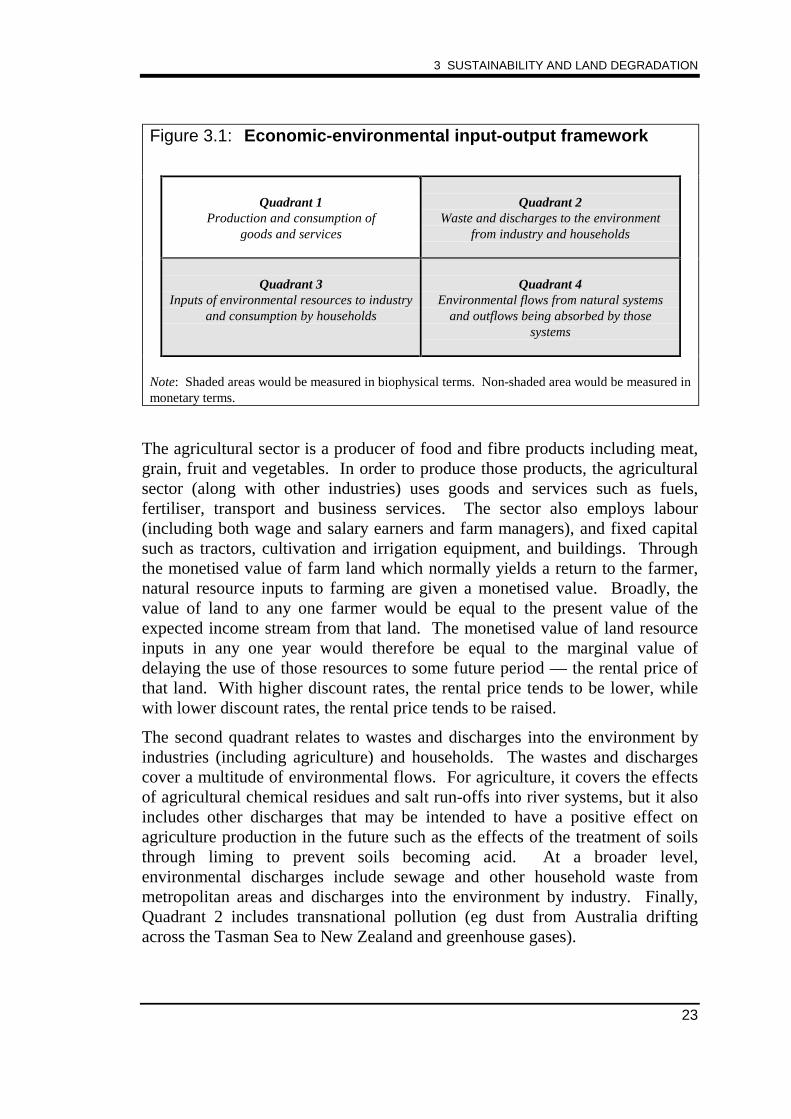
The concepts of intra-system functions and inter-system dependencies arecentral to the following discussion of agricultural land management. To makethe presentation of economic-environmental interactions clearer, the economicand environmental flows and the interaction between the two systems can beportrayed using a matrix presentation of inputs and outputs (see Figure 3.1).The matrix embodies both the monetary and physical aspects of the economic-environmental system.
The economic-environmental input-output matrix covers in its variouscomponents the inputs to industry (including agriculture, mining, manufacturingand services) and outputs from industry (such as wheat, wool, eggs and honeyfrom agriculture). Household use and investment are included to close thesystem. (The presentation of the matrix abstracts from inter-country flowsthrough imports and exports).
The model relates to economic and environmental flows and is divided into fourquadrants, reading from left to right, top to bottom, to capture the economic andenvironmental functions just discussed. In the first quadrant economic activityas conventionally reported in national accounting systems is shown (eg seeAustralian national income and expenditure accounts (ABS catalogueno. 5204.0) and input-output tables (ABS catalogue no. 5209.0). This economicactivity is expressed in monetary units of account and relates to the employmentof labour and capital by industry for the production of goods and services fordomestic use — by industry, households or capital accumulation — or export.When environmental flows have a recognised monetary value, those values areincluded in quadrant 1 as an input to production.4
4 Due to the interest and perceived importance of these flows for economic and
environmental management, they are formally included in a system of satellite accounts tothe internationally recognised System of National Accounts (Commission of the EuropeanCommunities, IMF, OECD, UN, and the World Bank 1993).
3 SUSTAINABILITY AND LAND DEGRADATION
23
Figure 3.1: Economic-environmental input-output framework
Quadrant 1Production and consumption of
goods and services
Quadrant 2Waste and discharges to the environment
from industry and households
Quadrant 3Inputs of environmental resources to industry
and consumption by households
Quadrant 4Environmental flows from natural systems
and outflows being absorbed by thosesystems
Note: Shaded areas would be measured in biophysical terms. Non-shaded area would be measured inmonetary terms.
The agricultural sector is a producer of food and fibre products including meat,grain, fruit and vegetables. In order to produce those products, the agriculturalsector (along with other industries) uses goods and services such as fuels,fertiliser, transport and business services. The sector also employs labour(including both wage and salary earners and farm managers), and fixed capitalsuch as tractors, cultivation and irrigation equipment, and buildings. Throughthe monetised value of farm land which normally yields a return to the farmer,natural resource inputs to farming are given a monetised value. Broadly, thevalue of land to any one farmer would be equal to the present value of theexpected income stream from that land. The monetised value of land resourceinputs in any one year would therefore be equal to the marginal value ofdelaying the use of those resources to some future period — the rental price ofthat land. With higher discount rates, the rental price tends to be lower, whilewith lower discount rates, the rental price tends to be raised.
The second quadrant relates to wastes and discharges into the environment byindustries (including agriculture) and households. The wastes and dischargescover a multitude of environmental flows. For agriculture, it covers the effectsof agricultural chemical residues and salt run-offs into river systems, but it alsoincludes other discharges that may be intended to have a positive effect onagriculture production in the future such as the effects of the treatment of soilsthrough liming to prevent soils becoming acid. At a broader level,environmental discharges include sewage and other household waste frommetropolitan areas and discharges into the environment by industry. Finally,Quadrant 2 includes transnational pollution (eg dust from Australia driftingacross the Tasman Sea to New Zealand and greenhouse gases).
STAFF INFORMATION PAPER
24
Quadrant 3 covers the use by industry and households of environmentalservices. The environment acts as a supplier of inputs to the agricultural sector(eg through water, minerals within the soil, fresh air, solar energy and light).Natural resource or environmental services used by this sector are conceptuallycovered within this part of the framework. The use of the environment by othersectors, such as mining and households is also covered by this quadrant.Quadrant 3 differs from quadrant 1 in that usage of environmental commoditiesis expressed in physical units of account. Therefore, to the extent that someresource flows are also monetised, Quadrant 3 overlaps with Quadrant 1. To theextent that resource and environmental amenity flows are not monetised,quadrant 3 complements quadrant 1.
Quadrants 1, 2 and 3, when taken together, represent a usage and distributionchain for the input of environmental resources into production and consumption,and the flow of residuals back to the environment. Industry sectors are linkedboth directly and indirectly to the environment. For example, for the farmingsector, lime which might be used to improve soil fertility is, at an earlier point inthe production and distribution chain, extracted from concentrations of thatmineral by the mining sector. This is also the case for other fertilisers. Waterused in irrigation is collected in high rainfall areas and transferred through waterdistribution networks to agricultural areas. Therefore, while the direct impact ofenvironmental activities can be focused on individual localities or regions, inthe presence of industrial specialisation and the capacity to transport goods andservices over long distances, the indirect effects are much more widespread.The household sector similarly has direct and indirect links to the environment.The economic and environmental activities of the agricultural sector can befully described within this economic-environmental framework.
Quadrant 4 is concerned with the natural functioning of environmental systems.It has no direct interaction with the economic production and distributionsystem. It includes an enormous range and diversity of bio-physical changesand functions from subtle changes in the earth’s surface brought about, forexample, by the movement of the tectonic plates to the natural functioning oflocalised forests and water courses. However, the ecological activity inQuadrant 4 is integrated with the rest of the extended economic-environmentalframework because economic development involves the increasingly intensiveuse of natural resources, and greater control over and pressure on the naturalenvironment (Quadrant 2). It is also integrated with the production andconsumption system as wastes and discharges from industry and householdsflow into natural systems and must be accommodated/absorbed in competitionwith other, naturally occurring, flows (Quadrant 3). Through environmentalflows conceptually covered in both quadrants 2 and 3, there can be a crowdingout of natural occurring systems. The changes to the environment may be
3 SUSTAINABILITY AND LAND DEGRADATION
25
beneficial to industrial productivity (which historically has been the norm).Nevertheless, changes may also reduce the utility of the environment for someaspects of industrial or household use, and for the continued functioning ofecological systems.
Because many environment services are not formally valued in the economy andlinks between the economy and the environment span many generations, the fulleconomic value of resources is not known. To overcome this information gap,it is tempting and, indeed appropriate, for the community to also determine thelevel and composition of ecological resources that the current generation wishesto bequeath to future generations.
3.3 Concepts and definitions
Concept of sustainable development
In 1980, the World Conservation Strategy was published by the InternationalUnion for Conservation of Natural Resources (IUCN) with advice andassistance from the United Nations Environment Programme (UNEP), WorldWildlife Fund (WWF), and in collaboration with the Food and AgriculturalOrganisation (FAO), and the United Nations Education, Science and CulturalOrganisation (UNESCO). This strategy was concerned with the maintenance ofessential ecological processes, the preservation of genetic diversity and thesustainable utilisation of species and ecosystems.
STAFF INFORMATION PAPER
26
In 1987, the concept of sustainable development was given further impetusworldwide through the report ‘Our Common Future’ issued by the WorldCommission on Environment and Development — the Brundtland Report, afterthe chairman of the Commission. The World Commission on Environment andDevelopment was established as an independent body in 1983 by a resolution ofthe United Nations General Assembly. The Brundtland Report focused on theinteractions between producers, consumers and the environment and concludedthat economic development and environmental protection are aspects of a singleoverall social management problem. Within this system of interactions, theconcept of sustainability does have limits imposed by technology, socialorganisation and the capacity of the environment to absorb the effects of humanactivity. The limits are not absolute in all cases, since there can be substitutionbetween human capital and natural resources and the regeneration of somenatural resources (eg soil fertility, forests). Thus, sustainability cannot bedefined according to predetermined bio-physical criteria. To capture the broadconcept of sustainability the Commission offered the following strategicdefinition:
Sustainable development is development that meets the needs of the present withoutcompromising the ability of future generations to meet their own needs. (WorldCommission on Environment and Development 1987, p. 43)
Finally, adoption of Agenda 21 (UNCED 1992) at the United NationsConference on Environment and Development (UNCED) held in Brazil in June1992 and the establishment of the United Nations Sustainable DevelopmentCommission signifies a high level of international commitment to theachievement of patterns of economic development which are sustainable.
Underlying international developments and interest in the links between theenvironment and economic development is the environmental input-outputframework and a realisation that there are limits to the flow of environmentalservices to production and consumption and the use of the environment for thedischarges of industry and households. However, economic-environmentrelationships are not static and a major influence on the potential for growth(including population growth and rising living standards) is technologicalchange and limits on substitution of environmental factors and man-madetechnologies.
The international consensus on actions adopted at the UNCED does not imposelegally binding commitments on governments or individual land managers toadopt sustainable land management practices. Although the UN SustainableDevelopment Commission will receive reports on environmental matters frommember countries, ultimately, the sustainable development practices would beadopted for domestic land management reasons.
3 SUSTAINABILITY AND LAND DEGRADATION
27
At the national policy level, the principles of ecological sustainabledevelopment have been enunciated in the National Strategy for EcologicallySustainable Development (ESD) (Commonwealth of Australia 1992). For thepurposes of that strategy, ESD is defined in the following way:
... using, conserving and enhancing the community’s resources so that ecologicalprocesses, on which life depends, are maintained, and the total quality of life, now andin the future, can be increased. (Commonwealth of Australia 1992, p. 6)
The essential message of this definition is the same as that provided by theWorld Commission. To provide an additional basis for the implementation ofAustralia’s national strategy, it establishes three core objectives:
• to enhance individual and community well-being and welfare by following a pathof economic development that safeguards the welfare of future generations;
• to provide for equity within and between generations; and
• to protect biological diversity and maintain essential ecological processes and life-support systems. (Commonwealth of Australia 1992, p. 8)
These are also very general guidelines which capture the concept of sustainabledevelopment and provide a basis for the development of an institutionalframework for sustainable development.
The management of agricultural land degradation and the Australian agriculturalindustry are embraced within the broad concept of ecological sustainabledevelopment (Ecologically Sustainable Development Working Group-Agriculture 1991 and Commonwealth of Australia 1991).
Definition of land degradation
Land degradation has negative connotations that imply the loss of something ofvalue. The lost value may be related to the productivity of the land foragriculture (the concern of this study), the environment as a host to naturallyoccurring species of flora and fauna, or the environment as a place for otherhuman activities (eg mining, secondary industries and human habitation or as anassimilator of wastes). Agricultural land degradation is significant because it:
• affects agricultural productivity;
• leads to the additional clearance of forests and native grasslands asexisting land loses productivity;
• places additional demands on other natural resources to repair the land (eglime for neutralising acidity, water for flushing irrigation salinity); and
• leads to off-site pollution and the loss of productivity and amenity values.
STAFF INFORMATION PAPER
28
The existence of such degradation provides a threat to the achievement ofnational ecologically sustainable development objectives.
Johnson and Lewis (1995) have noted that discussions of land degradation havetwo critical aspects, namely that there must be a substantial decrease in thebiological productivity of a land system and that the decrease is the result ofhuman activities rather than natural events. On this basis,
land degradation can be defined as the decline in the biological productivity orusefulness of land resources for their current predominant intended use caused throughthe use of the land by humans.
It encompasses soil degradation and changes in the traditional landscape andvegetation due to human interference. ‘Usefulness’ is a crucial attribute of landdegradation (National Soil Conservation Council (undated), McTainsh andBoughton 1993, Johnson and Lewis 1995). Declining usefulness of landresources indicates that human uses are crowding out pre-existing ecosystems ata rate above what would normally be expected in nature. The changes would beconsidered to be degradation once they impinge on the intended use of the landresources effected. As land resources have many possible uses with changes tothe landscape having both favourable and unfavourable effects depending onuse, the qualification ‘current predominant intended use’ is necessary in order tomake the definition of land degradation workable. Under this definition,desertification due to natural climate change would not be regarded asdegradation while desert-like conditions due to overgrazing or inappropriatetillage practices would.
However, degradation does not necessarily imply an immediate loss inproductivity. For example, biomass productivity could be maintained whiledegradation is present. This could occur during a period of overuse, so that thelonger-term ability of the soil to maintain production is diminished for short-term gain. It could also occur when human technological solutions allowfarming to co-exist with degradation (eg some areas of land may be sacrificed tosalinity to allow an otherwise very productive farming area to continueoperating).
While degradation has negative connotations, improving the condition of theland through land conservation has positive connotations. Land conservationcan be defined as: the prevention, mitigation and control of soil erosion andother forms of land degradation. Conservation is concerned with maintainingthe usefulness of the land and may be oriented to returning the land to someearlier natural condition or to maintaining its utility for farming, depending onthe intended use of the land. It may be achieved through retiring the land fromintensive use with a possible return to low input farming systems or conservingareas for native vegetation. The usefulness of the land can be maintained by
3 SUSTAINABILITY AND LAND DEGRADATION
29
substituting high yielding farming vegetation tolerant of the prevailing form ofdegradation (including tree crops), earthworks and land forming and other landmeasures, either singly or in combination, which enable the maintenance of landutility for future use.
Evaluation of the extent of land degradation also requires a benchmarkrepresenting the original condition of the land against which change can beevaluated. Conceptually, such a benchmark could be established with referenceto the condition of the land (represented in Quadrant 4 of the environmentalinput-output framework) in the absence of human production and consumptionactivities. Such a theoretical benchmark would be impracticable to determine,and possibly not very relevant to current land management decisions.Therefore, some arbitrary benchmark against which to assess the level andchange in land degradation must be chosen. In Australian studies, the arbitrarybenchmark generally chosen is the land condition that existed around 1800, tocoincide with the beginning of European settlement and the farming systemslinked to the modern economy. In this context, the modern economy ischaracterised by the interdependence of urban centres and rural communities,with the rural communities producing a surplus to meet the industrial andconsumer demands of urban populations in return for farm inputs and non-farmconsumer goods.
Rising demand has been met by human ingenuity in the use of natural resourcesand the substitution between natural and human capital. It is self evident thatthe process enables the utility of the land to be maintained for the production offood and rural products although there may be a loss of usefulness of land fornatural ecological systems. Notwithstanding increasing levels of output, therehave been catastrophes and costly errors of judgement which occur as part ofthe development of more productive farming systems (eg excessive andinappropriate tillage of the Victorian Mallee earlier this century). Agriculturalsystems that do not take advantage of ingenuity and technical progress, butrather rely on natural regeneration, would not be expected to provide the highestlevel of income now or in the future. In general, such farming systems arelikely to lack the potential to supply the broader community with sufficient foodto achieve and maintain basic nutritional requirements (see Figure 2.1 andWorld Commission on Environment and Development, 1987).
Types of land degradation
A multitude of causes contribute to the loss of value of land for human andecological purposes. Appendix A sets out in some detail a classification of landdegradation and measures of the severity of each form of degradation, whichhave been used by the Soil Conservation Service (SCS) of New South Wales in
STAFF INFORMATION PAPER
30
its 1987–1988 state-wide survey of land degradation and land use. Such acomprehensive classification, to which the Commission has added other types ofland degradation from other studies, provides a starting point for the linking ofdegradation to farm productivity and environmental issues.
Land degradation can involve the changing mineralisation of the soil, as occursthrough irrigation and dryland salinity, induced soil acidity and heavy metalcontamination of soils. Degradation can also involve changing soil structuresand erosion that occurs with soil structure decline, surface scalding, water andwind erosion and mass movement of slopes. Finally degradation of landresources can involve changes in biological conditions due to such factors aswoody shrub infestation, disappearance of perennial bush and the clearance ofnative vegetation, invasion by feral animals and other pest species, and pollutionfrom organic residues and farm wastes.
3.4 Land degradation and ecologically sustainabledevelopment
Land degradation of some form is likely to occur as human use of land becomesmore specialised and pressure on pre-existing natural environmental functions isincreased. The usefulness of the landscape for some environmental functions isreduced. In addition, specialised and successful farming systems may co-existwith some forms of degradation, such as irrigated agriculture and irrigationsalinity. An important question for the evaluation of sustainability is: will thegeneration of current income from agricultural land use and degradation todaylead to a permanent reduction in national productivity, and will essential lifesupport systems be threatened by the existence of degradation? If thedegradation is irreversible — or if it can only be reversed at an uneconomic cost— those land uses dependent on the availability of non-degraded land resourcesare not sustainable given current technologies.
Sustainable development can be achieved by the introduction of newtechnologies and the substitution of human capital for environmental resources,or by the conservation and replenishment of available resources for future use.In determining the options available to land managers, it is necessary todetermine whether individual land resources are renewable or depletable.Depletable natural resources are those whose replenishment is so slow that theycan be considered to be available for direct human use only once, such as topsoil in Australia, minerals and natural gas. For these resources, developmentcan only continue if new supplies/deposits are found or society has availablesome backstop technologies that can substitute for resource intensivetechnologies.
3 SUSTAINABILITY AND LAND DEGRADATION
31
By definition, renewable resources can be replenished over time; however, itshould be recognised that they can also be driven to extinction if the stockreaches some critical minimum required for regeneration or replenishment. Forexample, the Dodo bird was a renewable resource while a minimum breedingstock remained. Once that breeding stock was depleted, the species becameextinct. Many of the environmental impacts of agricultural activities can beclassed as renewable resources on the basis that repair periods of less than100 years are typical (Ecologically Sustainable Development Working Group-Agriculture 1991). In other cases, the natural repair period is so long that, forpractical purposes, damage could be deemed as permanent (eg loss of nativehabitats, flora and fauna).
Degradation occurs at a regional level and may be a threat to naturally occurringecological systems or to current farming systems. To evaluate environmentalquality in an economic and ecologically meaningful way, an appreciation isneeded of the biogeographic characteristics of each region, the land uses inthose regions and the extent of prevailing land degradation. A nation-widemeasure of environmental quality could then be obtained, taking into accountthe productivity of regions and regional ecologies.
In an effort to capture the biogeographic characteristic of regions at a nationallevel, the Australian Nature Conservation Agency (ANCA) has coordinated anational project to prepare the Interim Biogeographic Regionalisation ofAustralia (IBRA) (Thackway and Cresswell 1995). This classification builds onthe regional classifications developed by state land management authorities, inorder to divide Australia into regions according to biogeographic characteristics(see Appendix B). It has been used in this study to combine information aboutregional land use from the ABS census of agricultural establishments and theNew South Wales survey of land degradation (see Box 3.1).
While land degradation occurs at or is sourced to individual locations, there issubstantial diversity between the spacial range of degradation problems (andbenefits). A substantial number of degradation forms, such as soil structuredecline, induced soil acidity, surface scalding and water and wind erosion, relateto land resources at the farm level. There could be off-site (or external) effectsas soil run-off and nutrient loss induced by degradation enters the atmosphereand waterways. Nevertheless, other types of degradation have wider spacialranges. For example, dryland and irrigation salinity relate to underground watertables and acquifer systems that are not necessarily confined within theboundaries of individual farms, and for which the point of water inception isnormally remote from the point(s) of problem degradation. Off site, the effectscould be negative as the utility of the soils and waterways is reduced due to

STAFF INFORMATION PAPER
32
salting and nutrient run-off, but could also be positive with the increasedavailability of underground water for some farms.
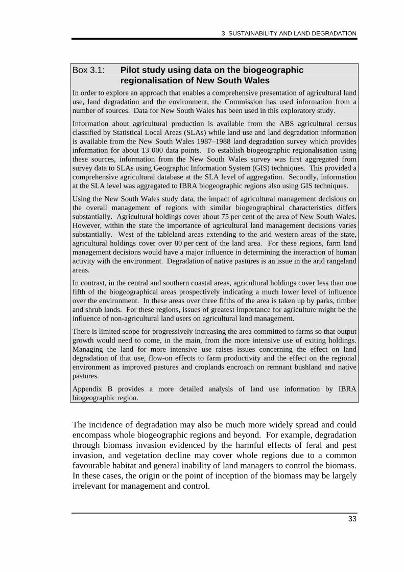
3 SUSTAINABILITY AND LAND DEGRADATION
33
Box 3.1: Pilot study using data on the biogeographicregionalisation of New South Wales
In order to explore an approach that enables a comprehensive presentation of agricultural landuse, land degradation and the environment, the Commission has used information from anumber of sources. Data for New South Wales has been used in this exploratory study.
Information about agricultural production is available from the ABS agricultural censusclassified by Statistical Local Areas (SLAs) while land use and land degradation informationis available from the New South Wales 1987–1988 land degradation survey which providesinformation for about 13 000 data points. To establish biogeographic regionalisation usingthese sources, information from the New South Wales survey was first aggregated fromsurvey data to SLAs using Geographic Information System (GIS) techniques. This provided acomprehensive agricultural database at the SLA level of aggregation. Secondly, informationat the SLA level was aggregated to IBRA biogeographic regions also using GIS techniques.
Using the New South Wales study data, the impact of agricultural management decisions onthe overall management of regions with similar biogeographical characteristics differssubstantially. Agricultural holdings cover about 75 per cent of the area of New South Wales.However, within the state the importance of agricultural land management decisions variessubstantially. West of the tableland areas extending to the arid western areas of the state,agricultural holdings cover over 80 per cent of the land area. For these regions, farm landmanagement decisions would have a major influence in determining the interaction of humanactivity with the environment. Degradation of native pastures is an issue in the arid rangelandareas.
In contrast, in the central and southern coastal areas, agricultural holdings cover less than onefifth of the biogeographical areas prospectively indicating a much lower level of influenceover the environment. In these areas over three fifths of the area is taken up by parks, timberand shrub lands. For these regions, issues of greatest importance for agriculture might be theinfluence of non-agricultural land users on agricultural land management.
There is limited scope for progressively increasing the area committed to farms so that outputgrowth would need to come, in the main, from the more intensive use of exiting holdings.Managing the land for more intensive use raises issues concerning the effect on landdegradation of that use, flow-on effects to farm productivity and the effect on the regionalenvironment as improved pastures and croplands encroach on remnant bushland and nativepastures.
Appendix B provides a more detailed analysis of land use information by IBRAbiogeographic region.
The incidence of degradation may also be much more widely spread and couldencompass whole biogeographic regions and beyond. For example, degradationthrough biomass invasion evidenced by the harmful effects of feral and pestinvasion, and vegetation decline may cover whole regions due to a commonfavourable habitat and general inability of land managers to control the biomass.In these cases, the origin or the point of inception of the biomass may be largelyirrelevant for management and control.
STAFF INFORMATION PAPER
34
The effects of land degradation also affect depletable resources (ie those thatcannot be regenerated or replenished). The loss of topsoil or depletion/pollutionof groundwater reserves is irreversible, for most practical purposes. In addition,the degradation of pre-existing environment through land clearance andcontemporary farming systems effectively replaces those systems based on thatpre-existing environment with new systems. Ultimately, ecological systemssubject to progressive replacement by utilitarian activities like farming could bedepleted. A similar picture applies to other land-using industries such asforestry, hunting and fishing. A different picture applies to the extractiveindustries within the mining sector, which by definition operates byprogressively discovering and depleting mineral deposits. Where agricultureuses fertilisers and additives to maintain soil fertility and structure, it is drawingon the output of the minerals sector. Accordingly, the sustainability of thoseagricultural systems is dependent on the output of the mining sector, which inturn depends on the continued availability of certain non-renewable minerals.
3.5 Farmer incentives and agricultural land degradation
At the individual farm level, action to prevent or ameliorate degradation is likelyto occur if the conservation effort and expense yield a positive stream of farmincome benefits. This would generally occur if the net present value of thenatural resource to the farmer justified the conservation costs givencommercially applicable discount rates. Economic analysis would suggest thatif such returns were not available, farm investment in conservation would not bewarranted.
Economic analysis would also suggest that in the absence of conservation effort,which is the case when a farmer simply mines land resources, farming wouldonly continue while a normal return on fixed capital could be obtained. As theland resource was degraded potential future profits would also be reduced untilultimately, that land would be retired from its degrading use in preference forsome other land use (Appendix D). As farmers must incur material, labour andcapital costs to farm the land, it is unlikely that resources on which farmingactivities depend would be totally depleted — it would not be profitable for thefarmer to do so. Totally depleted, is an extreme concept which in this contextmeans environmental resources are depleted to the point where theirregeneration and conservation is no longer possible (eg all topsoil is lost, soilsbecome poisoned and useless for farming).
The economic choices faced by individual farmers may however be somewhatmore subtle than indicated by these basic distinctions. While the sustainabilityof agricultural resource use may be bio-physically and economically achievable,
3 SUSTAINABILITY AND LAND DEGRADATION
35
the sustainable course of action may not be most profitable from the individualfarmer’s point of view. In evaluating expected returns, individual farmers mayhave several options yielding positive income streams once account is taken ofthe resale value of the property. Some of those options may in fact involveusing (mining) the land resource until the resource levels fall below theminimum required for agriculture. Other options may involveconservation/sustainable farming systems that yield a positive net income fromfarming in perpetuity. In the normal course of events, it would be expected thatthe farmer would choose the option that provided the largest net benefit. If thesustainability options are always the most profitable, it may be said thatagriculture is strongly sustainable (Pagiola 1993).
In other cases, the best alternative use may not be agriculture. For example,sustainable farming may be profitable in a region that is within an area beingrezoned for metropolitan and industrial use. That alternative use would mostprobably attach a land premium to locality rather than soil fertility. The bestoption for the farmer may be to mine the soil up to the point of sale of theproperty for that alternative use. On the other hand, the farmer could persistwith sustainable farming in the area and remain profitable as assessed againstthe cost of material, labour and fixed capital employed if, for his own reasons,he chose to do so. Competition from other alternative land uses such as, mineraldevelopment and retirement from agriculture on lease expiry (or termination)would afford the farmer similar non-conservation incentives.
The concept of sustainability is therefore most relevant where agriculture is thebest use of the land and is likely to remain so for the foreseeable future. Ingeneral some level of conservation farming affording sustainability ofagriculture would be justified in such regions.
The concept of sustainability is also not linked solely to the bio-physicalrequirements of agriculture and alternative land uses. Other factors could alsoinfluence farmer returns and decisions about land resource use. For example,expected declines in the agricultural terms of trade would lower the returns toagriculture relative to other activities given prevailing real discount rates. Itwould then pay farmers to bring forward output and sales effort and postponeconservation efforts. On the other hand, improvements in the terms of trade,would encourage current conservation efforts in order to take advantage ofexpected future real price increases, that is, the rate of growth of the resourcevalue would at least equal the real discount rate. Secondly, conservationexpenditure is one of a number of vehicles for raising the possible level offuture farm outputs. Research and development and changing farmtechnologies and productivity, also raise output potential but may notnecessarily reduce degradation. Some forms of new farming technologies such

STAFF INFORMATION PAPER
36
as feedlot farming may actually increase the levels of some forms ofdegradation such as soil structure decline. Other efforts may be directed at newfarming systems that co-exist with prevailing levels of degradation (eg thedevelopment and use of salt or acid tolerant plants). The yields to thecommunity from these alternatives may be greater than conservation farming,and therefore would be favoured by land managers.
From an individual farmers’ perspective, those forms of degradation that affectproductivity and profitability would be expected to be taken into account in theformation of farm plans and land management strategies. However, even iffarmers had full information concerning the environmental impact of theiroperations, there would remain environmental concerns to the community atlarge that would not be taken into account in farm plans in the normal course ofbusiness. Through the destruction of habitats having little utility forcontemporary agricultural systems, farming could reduce some natural resourcesdependent on those particular habitats below critical levels. For example, whereland clearing leads to the loss of native habitat within a biogeographic region.Secondly, the on-farm use of chemicals and irrigation water may normally beconsidered from the point of view of the individual farming enterprise ratherthan from the point of view of the broader community which takes account ofpotential downstream pollution of rivers and aquifers.
The link between farm productivity and environmental amenity is not entirelydecoupled as some polar interpretations of this distinction could suggest.Returning to the example of tree clearing, while clearing may not initially be anenvironmental issue for the farmer, over clearing can lead to reduced farmproductivity due to, for example, dryland salinity.
Another source of agricultural land degradation can come from the introductionof new farm systems that are intended to improve farm productivity and profitsthrough, amongst other things, reducing the adverse environmental effects ofearlier systems. For example, it is now well documented that improved pasturesand associated use of nitrogenous fertilisers were introduced to raise theproductivity of the land while at the same time reduce the incidence of soilerosion through better ground cover. Those farming systems have beensubsequently found to induce soil acidity, itself a cause of land degradation andlower farm productivity. In another example, chemical weedicides haveenabled a reduction in tillage and degradation through soil structural decline;however, the chemical run-off is a source of environmental pollution.
3 SUSTAINABILITY AND LAND DEGRADATION
37
3.6 A private or a social problem?
It is clear from the above discussion that land degradation cannot be treatedsolely as a problem for individual land-holders or for the current generation ofland managers. The costs of degradation and the benefits of preventing,ameliorating or repairing it facing individual land-holders will, in many cases,differ from the costs and benefits to the community as a whole.
Because the availability of land resources and the effects of conservation anddegradation cannot always be confined to individual holdings, conservation anddegradation will exhibit, to varying degrees, the characteristics of a public good(or bad):
• non-excludability — a potential land resource user cannot be denied accessto all of the land resources (including underground aquifer systems andwater basins) of a locality or region; and
• non-rivalry — a number of users can use a land resource (including‘goods’ such as rainfall but also ‘bads’ such as invasive plant and animalspecies) without changing its availability (or supply) to others in thelocality or region.
These characteristics focus first on the ability of individual farmers to containthe effect of conservation and degradation to their own land (ie the externalitiesof conservation and degradation) and, secondly, on the ability of other landmanagers to isolate themselves from degradation occurring in or originating onother land management areas in the same locality or region.
Forms of erosion such as sheet and rill erosion (a form of water erosion) andwind erosion, might generally be confined to the affected properties.Nevertheless, where declining land conditions cannot be practicably containedwithin a single holding, the land conservation actions of adjacent holdings maynot be fully effective in stopping the advance of the erosion. For irrigationsalinity and pest invasion it may be difficult for an individual land-holder in anaffected area to contain the effects within his property. Similarly, it may not bepossible for other land mangers to isolate themselves from the effects of theseforms of degradation or the conservation efforts of others.
It is clear that land resources and degradation cannot be treated as solely aproblem for individual land-holders. Frequently land resources and degradationspread beyond individual holdings to catchments and broader regions, so thateven on a group basis, land-holders do not necessarily perceive the full socialcosts of degradation.
The private and social division in the management of conservation anddegradation extends beyond the occurrence of land resources and the interaction

STAFF INFORMATION PAPER
38
between farmers in the use of those resources. The recognition and assessmentof land degradation, research towards a solution and implementation ofconservation plans is not costless and trade offs exist between farmer and socialeffort to find and implement conservation programs. To some extent, farmerlearning by doing may be sufficient to cope with a range of degradationproblems. Farm revenues would then cover the cost of such conservationefforts. However, research into land degradation problems that ultimatelybenefit communities of farmers would not be commercially justified by any oneindividual. This is due to the fact that individual farmers are not normally in aposition to appropriate the social benefits of their research to offset their privatecosts. Reliance on the research and development efforts of individual farmers,therefore, is likely to result in conservation efforts being less than the socialoptimum. This would be true even when the degradation problem is sitespecific, such as is the case with induced soil acidity. For this reason, research,development and land management information provided to the agriculturalsector also has public good characteristics (Industry Commission 1995a).
Thus, there are public good aspects and management issues in both theincidence, prevention and treatment of land degradation.
3.7 Conclusion
Broad concepts and principles have been established at the international andnational level for ecologically sustainable development. The agricultural sectoras a user of environmental resources provides one interface for the communitybetween its monetised system of production and consumption, and theenvironment. As the agricultural sector uses environmental resources some landdegradation will inevitably occur. The nature of degradation will change withchanges in technology associated with agricultural production and ourunderstanding of the environment.
Environmental expenditures and technological change make it possible toprevent or ameliorate degradation. However, the extent of the commitment ofresources to the prevention and amelioration of degradation is an empiricalquestion. It requires an examination of the extent of degradation, the costs andbenefits of repair from the community and farming points of view. It alsorequires an appreciation of the incentives facing farmers in their choice offarming systems.
39
CHAPTER 4ECONOMIC EFFECTS OF LAND DEGRADATIONIN AUSTRALIA
4.1 Introduction
The concept of land degradation implies some deterioration in land quality. Theloss in productivity reflects the economic costs of degradation. However,positive economic costs do not necessarily lead to conservation activities toreduce degradation. There are links between levels of degradation, productionand profit and therefore a trade-off exists between higher production anddegradation.
This chapter considers the economic effects of land degradation in Australia andthe costs and benefits of ameliorating activities. Section 4.2 focuses on theextent of land degradation in Australia. Section 4.3 reports selected estimates ofthe production foregone due to degradation and summary results from severalcost-benefit analyses. Section 4.4 outlines the main findings of a Commissionstudy of New South Wales agriculture undertaken to explore the links betweenproduction, profit and degradation.
4.2 The extent of land degradation in Australia
Introduction
The Commission investigated the extent of land degradation in Australia withtwo objectives in mind. The first objective was to investigate land degradationin New South Wales using information from the 1987–1988 SCS landdegradation survey. The aim of this work was to assess whether the informationcould be successfully incorporated into a state-wide model of New South Walesagriculture in order to provide a broad view of degradation and the stateagricultural industry.
The second objective was to undertake a preliminary collection of landdegradation information from the New South Wales and other studies tobroaden the view of land degradation in Australia.
STAFF INFORMATION PAPER
40
Broad picture of degradation
State-wide studies
The Commission has found that there is a long-standing active interest ininvestigating the extent of land degradation. This interest is reflected inpublished results for states as a whole, detailed studies of localities and regionswithin states and individual forms of degradation (see Appendix C). However,while each exercise contains valuable land degradation information for thearea/degradation type under study, integrated nation-wide information islacking.
So far only one national degradation assessment study has been carried out(Woods 1983). This survey, conducted by the Commonwealth and States in acollaborative study of soil conservation over the period 1975 to 1977, focusedon appraising the incidence of land requiring treatment rather than providing aninventory of land degradation. Such an inventory would have had the addedadvantage that it could have been used to assess the effects of degradation or asa benchmark against which future appraisals could be compared. Nevertheless,as it was, the study estimated that a total of about 80 million hectares, or16 per cent of agricultural land required some form of treatment. Over two-thirds of the problems related to water erosion with New South Wales havingthe highest concentration of this problem (around 24 million hectares). Largeareas of vegetation decline (eg woody shrub infestation) were also recorded asrequiring treatment in Queensland, New South Wales and the NorthernTerritory.
Although a national study has not been repeated, more recent data on the extentof land degradation for individual states is available. This information paperhas referred to data for New South Wales, Victoria, Western Australia andTasmania. Each report shows that a number of types of degradation affectsubstantial portions of the states considered.
For New South Wales, the 1987–1988 survey considered the extent and severityof ten forms of land degradation. Over 10 per cent of the land area in that statewas estimated to be affected by severe soil structure decline or gully erosion,while around 4 per cent suffered from severe induced soil acidity and woodyshrub infestation. Severe vulnerability to wind erosion has affected around11 per cent of the land whereas severe vulnerability to sheet and rill erosion (aform of water erosion) affected less than 1 per cent. Around 1 per cent of thestate is also affected by severe salinity. Nevertheless, for each form ofdegradation considered, over three quarters of the state has nil or minor levels ofland degradation.
4 ECONOMIC EFFECTS OF LAND DEGRADATION IN AUSTRALIA
41
The process of assessing the nature and severity of land degradation changessubstantially over time. New forms of degradation emerge and previouslyrecorded forms of degradation receive less attention. For example, the 1967SCS survey of New South Wales land degradation examined only gully, sheetand wind erosion whereas the 1987–1988 survey included those forms oferosion with a much larger range of degradation types. By comparison, the later1987–1988 survey included in its coverage less visible forms of degradation,such as soil structure decline and induced soil acidity.
Studies of land degradation in Victoria indicate a substantial reduction in waterand wind erosion over the years, to the point where the area subject to theseforms of erosion is small compared to the total area of agricultural land.However, other forms of degradation such as induced acidity and soil structuredecline are now assessed to be very widespread. For example, 58 per cent ofdryland pasture is extremely acidic and around 40 per cent of broadacre cropland and 90 per cent of irrigated pasture have severe soil structure decline.Irrigation salinity occurs in one fifth of the area of irrigated pasture andhorticultural land, while dryland salinity occurs in about 1 per cent ofagricultural holdings in Victoria. Based on the area affected, salinity appears tobe less of a problem in Victoria than acidity and soil structure decline.
The most extensive forms of land degradation in Western Australia arevegetation decline and erosion in the rangelands which affects about 8 per centand 3 per cent of the total area of this state, respectively. Of degradationassociated with lands used for cropping and improved pasture, soil structuredecline is the most widespread problem in Western Australia, affecting up to7 per cent of the state. While the reported area of dryland salinity was only0.2 per cent of the state, it is a potentially serious form of degradation becausepotential saline areas are concentrated in the more productive south-westerncoastal areas and the area of saline land could increase five-fold to around1 per cent of the state.
For Tasmania, a survey of degradation on private freehold land was conductedover the years 1992 and 1993. Eight forms of degradation were examined.Taken together, the survey found that almost all private land suffers from someform of degradation. However, when each form of degradation, other than treedecline, is considered individually, it was found that over 80 per cent of privatefreehold land has nil or minor degradation of the type under consideration. Forexample, 85 per cent of freehold land was assessed as having nil to minor soilstructure decline while only one per cent of the land was assessed as havingsevere soil structure decline. For tree decline (eg die-back of foliage), thesurvey found that 40 per cent of private land was affected by moderate toextreme degradation. The least common form of degradation on private land
STAFF INFORMATION PAPER
42
was tunnel erosion for which 5 per cent of land was affected by shallow to deeptunnels.
Overall, the state-wide results cannot be easily compared. Nevertheless, thecoverage of each of the studies to include the less visible forms of degradationsuch as soil structure decline, induced soil acidity and dryland salinity indicatesthat these substantially on-farm forms of degradation are now consideredimportant land management issues along with the more traditional forms ofwind and water erosion. Obviously irrigation salinity is confined to irrigationareas and adjacent areas sharing common underground water systems.
Studies of particular regions or forms of degradation
While state or nation-wide studies can provide a broad picture of degradation, inorder to fully understand degradation and its advance, it is necessary to look inmore detail at individual locations or regions, and at individual forms ofdegradation.
There are a number of studies that have done this. The Commission hasconsidered studies relating to irrigation salinity in the Murray-Darling Basin,dryland salinity across Australia and soil acidification (see Appendix C).
The studies indicate that under current land management practices these types ofdegradation will continue to advance. For example, irrigation salinity couldincrease over the next 30 to 50 years in the Riverine Plains Zone of the DarlingBasin, spreading at rates of between 1 per cent and 3 per cent (per annum)during the 1990s. Estimates of the rates of increase for dryland salinity are notavailable, however across Australia the current level affected is estimated to behalf of the potential level. Degradation from induced soil acidity could advanceat between 0.2 per cent and 1 per cent (per annum) in New South Wales,depending on soil types.
Comparability of studies
One concern for the development of an overall view of degradation and itsseverity is the substantial differences between the estimated areas affected bydegradation provided by the various detailed studies and the state-wide reports(see Appendix C). For example, the New South Wales SCS survey estimatedthat induced soil acidity (ranging from severe to highly acidic) affected around2.8 million hectares whereas an AACM (1995) study found that there werearound 13.5 million hectares of highly acid soils in New South Wales.However, for Victoria, the state study estimate of strong and extremely acid soilis 4.6 million hectares compared to the AACM estimate of 3 million hectares.In the case of dryland salinity a similar variable estimate is provided from acomparison of possible sources. In Victoria, the Land and Water Resources
4 ECONOMIC EFFECTS OF LAND DEGRADATION IN AUSTRALIA
43
R&D Corporation et al. (1992) analysis reported an estimated 135 thousandhectares of area affected, whereas the state report estimated 100 thousandhectares. In addition, data for New South Wales and Western Australia differedbetween sources.
In principle, it should be noted that the different estimates reflect the incidenceof more intensive surveys, improvements in recognising the occurrence ofdegradation, different reference periods and different definitions. Thus,technical explanations could describe the somewhat different pictures ofdegradation provided by the different analyses. To take a forward looking landmanagement perspective, an integrated and consistent view of the extent ofdegradation and its advance, would require comprehensive and consistent datasources assembled for common reference periods.
A closer look at land degradation survey information for New SouthWales
The predominantly location specific nature of land degradation necessitates adetailed understanding of the incidence and severity of the problem at sitelevels. With this in mind, the Commission analysed the New South Wales1987–1988 survey data to obtain a regional disaggregation of land degradation.The 13 000 data points included in the survey were grouped into 185 StatisticalLocal Areas (SLAs) and an index of degradation was estimated for each of the149 SLAs with substantial agricultural activity (see Appendixes B and C). Acomposite index for all degradation types shows that the SLAs with the highestlevels of degradation lie in an area extending from Goulburn in the SouthEastern Highlands across SLAs in the South Western Slopes to the Riverina.
Of the ten types of degradation surveyed, four types — irrigation salinity,dryland salinity, induced soil acidity and soil structure decline — were selectedfor further analysis. For each of these types, separate indexes of degradationwere estimated by SLA. The index results indicate substantial differences in theincidence of degradation across SLAs (see Figure 4.1). For both irrigation anddryland salinity, severe degradation is clustered into a small group of SLAs. Inboth cases, there is another small group of SLAs with moderate salinity. Themost severe dryland salinity extends from SLAs in the Sydney Basin across theSouth Eastern Highlands to the South Western Slopes. These regions tend tohave higher rainfall, high levels of cleared land and sloping countryside, all ofwhich make them more susceptible to dryland salinity than other SLAs in NewSouth Wales. Irrigation salinity, as expected, is concentrated in the irrigationareas of the Riverina.
STAFF INFORMATION PAPER
44
The incidence of induced soil acidity and structure decline, on the other hand, ismuch more widespread. About one-third of SLAs are affected by severe acidityand they fall in the biogeographical regions of the Sydney Basin, South EasternHighlands, South Eastern Slopes and Riverina. However, there is a substantialgroup of SLAs poised with a high incidence of potential problem acid soils.Soil structure decline is even more prevalent and it is focussed in areas withinthe regions of the Sydney Basin, South Western Slopes and Riverina. There isalso a substantial group of SLAs with moderate structural decline.
An important longer-term issue in understanding the processes of degradation,concerns the combination of farm management decisions and regionalbiogeographical characteristics that characterise the grouping of SLAsexhibiting potential induced soil acidity and moderate soil structure without alsoexhibiting severe cases of these forms of degradation. Are these SLAs intransition to more severe degradation , or is there biogeographic and landmanagement reasons why severe degradation was not observed or has beenavoided?
Of these four degradation types, the most widespread are those that are largelyfarm specific, that is, induced soil acidity and soil structure decline. Irrigationsalinity which could impose substantial external effects on others, is highlyconcentrated at the regional level.
4.3 Production loss from land degradation and cost-benefitanalysis of amelioration works
Implicit in the concept of land degradation is the notion that agricultural landuse removes some useful ingredients from the land bringing about adeterioration in its quality and reducing its productivity. To assess the impact ofland degradation, it is relevant to estimate the loss in economic value due todegradation. Two approaches have been traditionally followed. One approachis to estimate the potential productivity of the land, without degradation, in itscurrent use. The concept of a ‘production equivalent of degradation’ is useful intranslating a measure of the incidence of degradation into a standardisednumeraire, that is, dollars of production or revenue. The other approachinvolves analyses of the cost of repair and conservation activities and futurebenefits expected from those activities.
A number of studies report estimates of the production equivalent ofdegradation. They range from a national average of 5 per cent of the value ofagricultural production for all types of degradation to 6 per cent for sheet andrill erosion alone in the Lachlan catchment of New South Wales (see
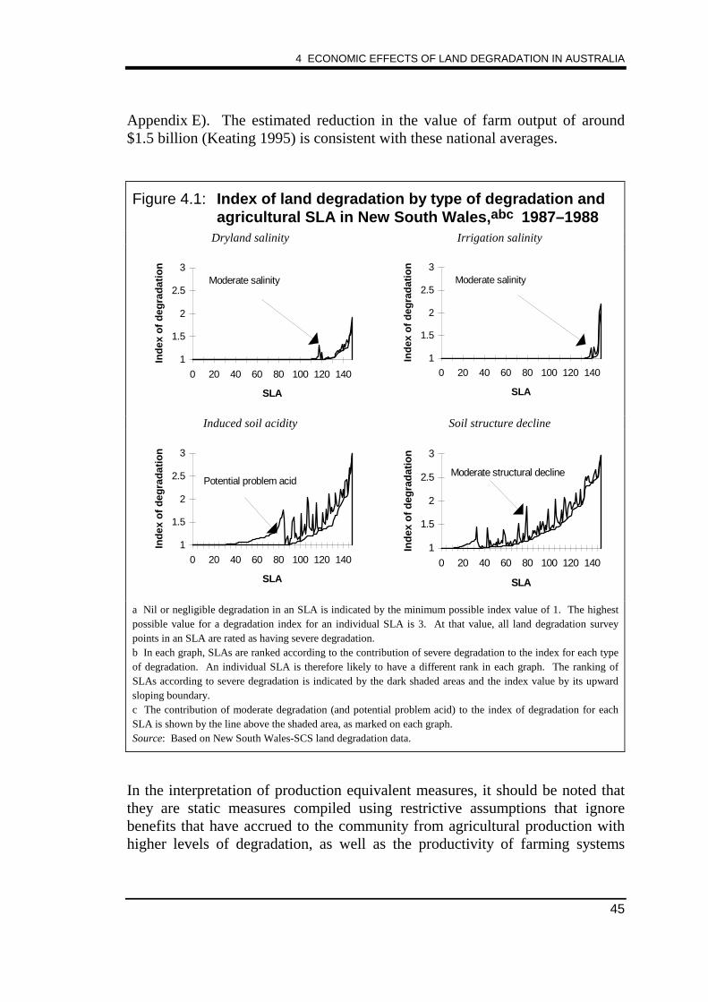
4 ECONOMIC EFFECTS OF LAND DEGRADATION IN AUSTRALIA
45
Appendix E). The estimated reduction in the value of farm output of around$1.5 billion (Keating 1995) is consistent with these national averages.
Figure 4.1: Index of land degradation by type of degradation andagricultural SLA in New South Wales,abc 1987–1988
Dryland salinity Irrigation salinity
1
1.5
2
2.5
3
0 20 40 60 80 100 120 140
SLA
Ind
ex o
f d
egra
dat
ion
Moderate salinity
1
1.5
2
2.5
3
0 20 40 60 80 100 120 140
SLA
Ind
ex o
f d
egra
dat
ion
Moderate salinity
Induced soil acidity Soil structure decline
1
1.5
2
2.5
3
0 20 40 60 80 100 120 140
SLA
Ind
ex o
f d
egra
dat
ion
Potential problem acid
1
1.5
2
2.5
3
0 20 40 60 80 100 120 140
SLA
Ind
ex o
f d
egra
dat
ion
Moderate structural decline
a Nil or negligible degradation in an SLA is indicated by the minimum possible index value of 1. The highestpossible value for a degradation index for an individual SLA is 3. At that value, all land degradation surveypoints in an SLA are rated as having severe degradation.b In each graph, SLAs are ranked according to the contribution of severe degradation to the index for each typeof degradation. An individual SLA is therefore likely to have a different rank in each graph. The ranking ofSLAs according to severe degradation is indicated by the dark shaded areas and the index value by its upwardsloping boundary.c The contribution of moderate degradation (and potential problem acid) to the index of degradation for eachSLA is shown by the line above the shaded area, as marked on each graph.Source: Based on New South Wales-SCS land degradation data.
In the interpretation of production equivalent measures, it should be noted thatthey are static measures compiled using restrictive assumptions that ignorebenefits that have accrued to the community from agricultural production withhigher levels of degradation, as well as the productivity of farming systems
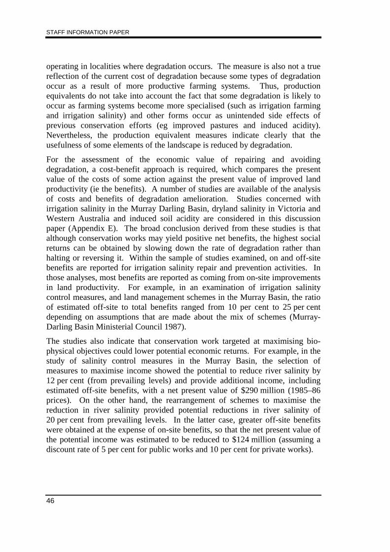
STAFF INFORMATION PAPER
46
operating in localities where degradation occurs. The measure is also not a truereflection of the current cost of degradation because some types of degradationoccur as a result of more productive farming systems. Thus, productionequivalents do not take into account the fact that some degradation is likely tooccur as farming systems become more specialised (such as irrigation farmingand irrigation salinity) and other forms occur as unintended side effects ofprevious conservation efforts (eg improved pastures and induced acidity).Nevertheless, the production equivalent measures indicate clearly that theusefulness of some elements of the landscape is reduced by degradation.
For the assessment of the economic value of repairing and avoidingdegradation, a cost-benefit approach is required, which compares the presentvalue of the costs of some action against the present value of improved landproductivity (ie the benefits). A number of studies are available of the analysisof costs and benefits of degradation amelioration. Studies concerned withirrigation salinity in the Murray Darling Basin, dryland salinity in Victoria andWestern Australia and induced soil acidity are considered in this discussionpaper (Appendix E). The broad conclusion derived from these studies is thatalthough conservation works may yield positive net benefits, the highest socialreturns can be obtained by slowing down the rate of degradation rather thanhalting or reversing it. Within the sample of studies examined, on and off-sitebenefits are reported for irrigation salinity repair and prevention activities. Inthose analyses, most benefits are reported as coming from on-site improvementsin land productivity. For example, in an examination of irrigation salinitycontrol measures, and land management schemes in the Murray Basin, the ratioof estimated off-site to total benefits ranged from 10 per cent to 25 per centdepending on assumptions that are made about the mix of schemes (Murray-Darling Basin Ministerial Council 1987).
The studies also indicate that conservation work targeted at maximising bio-physical objectives could lower potential economic returns. For example, in thestudy of salinity control measures in the Murray Basin, the selection ofmeasures to maximise income showed the potential to reduce river salinity by12 per cent (from prevailing levels) and provide additional income, includingestimated off-site benefits, with a net present value of $290 million (1985–86prices). On the other hand, the rearrangement of schemes to maximise thereduction in river salinity provided potential reductions in river salinity of20 per cent from prevailing levels. In the latter case, greater off-site benefitswere obtained at the expense of on-site benefits, so that the net present value ofthe potential income was estimated to be reduced to $124 million (assuming adiscount rate of 5 per cent for public works and 10 per cent for private works).
4 ECONOMIC EFFECTS OF LAND DEGRADATION IN AUSTRALIA
47
Achieving some predetermined bio-physical objective may not be economicallyfeasible once account is taken of the costs and benefits to agriculture. Forexample, a cost-benefit analysis concerned with the control of dryland salinity inthe Neridup catchment, located north-east of Esperance in Western Australia,finds that a negative marginal benefit would be likely as the rate of advance ofdegradation was targeted to zero (see solid line in Figure 4.2). Assuming thattrees planted to aid in arresting salinity could not be harvested commercially, themaximum net benefit to farmers was estimated to occur when the spread ofdryland salinity is reduced from 88 hectares per year to around 50 hectares peryear. The study also considered the sensitivity of the results to the introductionof commercial forestry. The introduction of commercial forestry was found toreduce the profit maximising rate of spread of degradation from around50 hectares per year to around 40 hectares per year (see broken line, Figure 4.2)
There is a fair degree of variation in the cost-benefit methodologies adopted inthe studies examined. One common feature is the adoption of a real socialdiscount rate to estimate the present value of future streams of costs andbenefits. Because of the adoption of different discount rates, over different timeperiods and for different regions, comparison between studies is not possible, orindeed appropriate.
Figure 4.2: Marginal net benefits from controlling dryland salinitywith and without commercial treesab
-250
-200
-150
-100
-50
0
50
100
150
88 80 70 60 50 40 30 20 10 0
Mar
gin
al b
enef
its
(do
llar
per
h
ecta
re)
Without commercial trees
With commercial trees
Rate of spread of salinity (hectare per year)
a To obtain net benefits, the standard cost benefit approach of comparing cash flows resulting from present farmmanagement practices with cash flows resulting from conservation strategies was adopted.b The reference (or ‘current’) rate of spread of dry land salinity is 88 hectares per year. This is the benchmarkrate of spread for the study.Source: Campbell (1994).
STAFF INFORMATION PAPER
48
Another common feature is the assumption that relative prices are unchanged.Under this assumption, the methodologies capture changes in the volume ofinputs (costs) and outputs (benefits) arising from degradation repair andprevention activity. However, for any given discount rate, they do not capturethe effects of relative price changes. A change in the terms of trade would alterthe attractiveness of agricultural activities compared to other activities in theeconomy, and hence the attractiveness of investing in agriculture through forexample, land degradation repair and prevention.
With no changes in the terms of trade, the money values of a unit of outputwould purchase the same bundle of materials, labour and capital inputs in thefuture as in the current period. With declining terms of trade, the money valueof a unit of output would buy fewer inputs in the future. With an improvementin the terms of trade, additional inputs could be purchased with a unit of outputor profits could be increased. Possible changes in the relative value of industryoutputs, relative to the costs of inputs is not explicitly taken into account bydiscounting so that when no explicit adjustment is made for changes in relativeprices, it is assumed that cost benefit analyses reflect constant relative prices.
In the presence of declining terms of trade, as has typified Australianagriculture, the methodologies adopted could overstate the possible neteconomic benefits to the community of environmental conservation projects.By the same token, were the agricultural terms of trade to improve in the future,the method would have the opposite bias and understate possible benefits.
Generally, it has not been possible to provide cost-benefit estimates revised totest the sensitivity of results to possible terms of trade changes. However, forthe study into the reduction of induced soil acidity (AACM 1995 discussed inAppendix E), a re-estimation of the benefits of liming (ie a standard treatmentfor problem acid soils) has been possible. The original study suggests that overa 15 year period (with a real discount rate of 10 per cent), the net financialbenefits of liming for wheat production in the Western Slopes of New SouthWales has been estimated at $206.50 per hectare with constant terms of trade.Providing for the possible continued decline in agricultural terms of trade, thisnet benefit would be reduced to $114 per hectare. Industry outlook couldtherefore have a substantial impact on farmers assessment of land managementstrategies, given some standard commercial real discount rate.
The problem with off-farm effects of degradation is the inability of otherresource users to exclude themselves from those effects (at least withoutadditional costs to themselves). Some studies do take into account the off-siteeffects of degradation and conservation effort on the productivity of othereconomic activities. Where this is done, off-site benefits vary in importance.For example, a series of land management schemes to control irrigation salinity
4 ECONOMIC EFFECTS OF LAND DEGRADATION IN AUSTRALIA
49
in the Murray-Darling Basin were ranked to maximise, on one hand, communityincome and on the other a reduction of river salinity. These provided netbenefits of $626 million and $420 million (1986 prices) respectively (seeAppendix E). The first group of projects obtained 90 per cent of the totalestimated benefits from local farm based improvements in productivity whereasthe second group of projects obtained only 75 per cent of benefits from farm-based projects with the remaining benefits, in both cases, coming from lowerriver salinity. In a broad economic context, an ecological target of lower riversalinity could therefore be obtained by the community by forgoing agriculturalincome from the farming region.
Overall, the studies considered are oriented towards an economic analysis of thecosts and benefits of conservation activities that may occur in an individuallocality or region. Where appropriate, the external effects of those activities areincorporated in the analysis. The analyses indicate that most of the benefit fromdegradation repair and prevention activities would accrue to the communitythrough on-farms returns, even for irrigation salinity projects. Due to thelocality specific nature of land degradation, it would be useful to examineimpediments to farmer involvement in conservation programs that benefit them.
4.4 An analysis of the state-wide effects of land degradation inNew South Wales
Introduction
To make a start towards establishing a state-wide empirical framework foranalysing degradation, the Commission has estimated a model of New SouthWales agriculture incorporating land degradation. The model uses a snapshot,or a cross section, of the New South Wales agricultural economy in the early1990s to study the effects of four forms of degradation: irrigation salinity,dryland salinity, soil structure decline, and induced soil acidity. The estimatedeffects of degradation on production and profits represent a medium to longer-run perspective. An overview of the model is provided in Box 4.1, while detailsof the model specification and results are provided in Appendix F. Thebiogeographic regionalisation used in the model estimation is discussed inAppendix B.
STAFF INFORMATION PAPER
50
Box 4.1: The Commission’s econometric model of New SouthWales agriculture
The effects of land degradation are examined using a model of agriculture in New SouthWales developed by the Commission. This is an econometric model that is based on theprofit-maximising behaviour of individual farmers.
It is assumed that farmers’ choose both their input and output mixes to maximise profits givena level of fixed factors of production and prevailing levels of land degradation. Thisassumption is suited to the analysis of the Australian agricultural sector, which has manyproducers each having little control over the input and output prices but with each having theopportunity to vary their input and output mixes. Because the model is state-wide, it capturesin aggregate, a snapshot of the production decisions of all farmers and provides an overview(or state-wide) assessment of agriculture and the effects of degradation.
The model evaluates the responses of farmers to changing conditions on the basis of a cross-section of New South Wales agricultural industry data disaggregated into 149 SLAs.Analytical results therefore are based on a comparison of the variability in farmer responses torelative price changes, given land, labour and degradation constraints. The modelincorporates two commodity output categories: crops and other plant products (crops); andanimals and animal products (animal products). It also contains variable inputs divided intofour categories, namely: hired labour; fertiliser; water (including water rates); and othermaterials and services (the numeraire for the model). The fixed factors of production are: thearea of agricultural land holdings; and farmer and farm manager labour; while degradation isanalysed with reference to: dryland salinity; irrigation salinity; soil structure decline; andinduced soil acidity.
In order to account for regional differences in production and income due to interregionalbiogeographical features, the following seven New South Wales regional dummy variableswere included in the model: North Coast; Central and South coast; Tablelands; Central areas;Central-west areas; Western areas; and Irrigation areas.
The model implicitly takes into account the opportunity cost of land degradation to individualfarmers. Within its framework, farmers are treated as choosing between either production inthe current period at the expense of additional degradation, or lower levels of production atsome future, indeterminate, time and less degradation in the current period. Because data aredrawn from a cross-section of state agriculture, the estimated effects of degradation onproduction and profits have a medium to longer-run perspective, even though only data fortwo years are used.
Production, input and price data are drawn from a combination of ABS and ABARE datasources. The reference years for the analysis are 1991–92 and 1992–93. Land degradationdata used in the model were taken from the 1987–1988 Survey of Land Degradationconducted by the SCS of New South Wales. Because of the slow advance of degradation,using data for this earlier year is deemed to provide a useful proxy of the regional intensitiesof degradation.
The specification of the model, model results and data sources are discussed in detail inAppendix F. The biogeographic regionalisation of New South Wales is discussed inAppendix B.
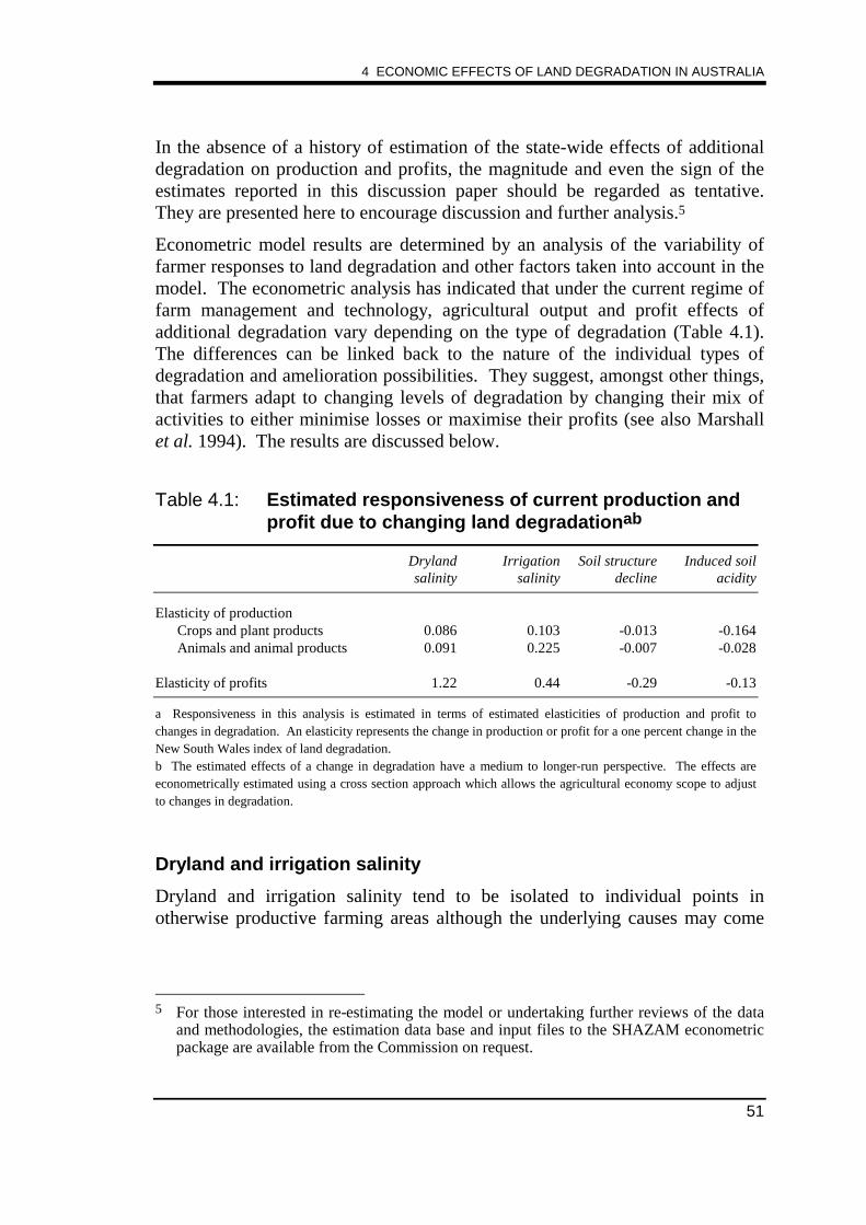
4 ECONOMIC EFFECTS OF LAND DEGRADATION IN AUSTRALIA
51
In the absence of a history of estimation of the state-wide effects of additionaldegradation on production and profits, the magnitude and even the sign of theestimates reported in this discussion paper should be regarded as tentative.They are presented here to encourage discussion and further analysis.5
Econometric model results are determined by an analysis of the variability offarmer responses to land degradation and other factors taken into account in themodel. The econometric analysis has indicated that under the current regime offarm management and technology, agricultural output and profit effects ofadditional degradation vary depending on the type of degradation (Table 4.1).The differences can be linked back to the nature of the individual types ofdegradation and amelioration possibilities. They suggest, amongst other things,that farmers adapt to changing levels of degradation by changing their mix ofactivities to either minimise losses or maximise their profits (see also Marshallet al. 1994). The results are discussed below.
Table 4.1: Estimated responsiveness of current production andprofit due to changing land degradationab
Drylandsalinity
Irrigationsalinity
Soil structuredecline
Induced soilacidity
Elasticity of production Crops and plant products 0.086 0.103 -0.013 -0.164 Animals and animal products 0.091 0.225 -0.007 -0.028
Elasticity of profits 1.22 0.44 -0.29 -0.13
a Responsiveness in this analysis is estimated in terms of estimated elasticities of production and profit tochanges in degradation. An elasticity represents the change in production or profit for a one percent change in theNew South Wales index of land degradation.b The estimated effects of a change in degradation have a medium to longer-run perspective. The effects areeconometrically estimated using a cross section approach which allows the agricultural economy scope to adjustto changes in degradation.
Dryland and irrigation salinity
Dryland and irrigation salinity tend to be isolated to individual points inotherwise productive farming areas although the underlying causes may come
5 For those interested in re-estimating the model or undertaking further reviews of the data
and methodologies, the estimation data base and input files to the SHAZAM econometricpackage are available from the Commission on request.
STAFF INFORMATION PAPER
52
from underground water tables, aquifer systems and regional farming practices.6This confinement of problem salinity would lend support to the notion thatfarmers could be drawn into high levels of land clearance in areas susceptible todryland salinity and to irrigation farming even at the expense of some additionalsalinity problems. This may be particularly so when the farms undertakingclearing or irrigating highly productive lands will not necessarily be the samefarms that experience the problem salinity.
Consistent with this perspective, the econometric estimates indicate that higherlevels of production could be achieved by a shift toward farming activities thatare characterised by higher levels of dryland or irrigation salinity. A shiftentailing a 1 per cent increase in the index of degradation due to dryland salinityis projected to raise crop and animal production by around 0.09 per cent withcrops increasing fractionally more than animal products. A 1 per cent increasein the index of degradation due to irrigation salinity is projected to raise cropand animal production by around 0.1 per cent and 2.3 per cent, respectively.
While there may be incentives to move towards farming activities that areassociated with higher levels of these forms of degradation there are alsoincentives to adapt farming practices to minimise the adverse effects of suchdegradation in areas where it is most severe. Adaptation to irrigation anddryland salinity involves land management strategies that reduce wateraccessions and favour salt resistant crops and pastures. One way for farmers toachieve this is to vary the mix of crops and livestock in farm output. Theeconometric results tentatively suggest that livestock products would befavoured over crop products. Many factors could be at work in determiningthis. In the case of dryland salinity, which tends to occur in hillier areas, wateraccessions may be reduced and water tables controlled by the introduction ofdeep-rooted perennial plants, such as lucerne. When these pastures are grazeddirectly, higher livestock output could occur. On the other hand, whereplantings are cut for hay, crop production (inclusive of lucerne and grass hay)would be favoured. The estimates suggest that cropping may have a slightadvantage over grazing activities. In the case of irrigation salinity, asubstitution from cropping to grazing activities has been estimated to occur asthe severity and extent of irrigation salinity increases. This result is consistentwith farming strategies that lower water accessions and control water tables bysubstituting less irrigation intensive and salt sensitive grazing activities for moreirrigation intensive and salt sensitive cropping activities. 6 The characteristic of these forms of degradation led the New South Wales Soil
Conservation Service to publish measures of dryland and irrigation salinity in terms of thepercentage of land degradation survey data points affected by degradation rather than interms of the area affected. The estimation of land degradation indexes and a furtherdiscussion of this problem is provided in Appendices C and F.
4 ECONOMIC EFFECTS OF LAND DEGRADATION IN AUSTRALIA
53
Overall, the projected increases in production and profits from higher levels ofdryland and irrigation salinity indicate that, at the current level of developmentof the agricultural industry in New South Wales, there are incentives for farmerswho are operating with evident salinity not to move away from those farmingactivities. The regional groupings identified with these farming incentiveswould have moderate to severe degradation as identified in Figure 4.1.Similarly, there are incentives for other farmers to move towards those farmingactivities that co-exist with higher levels of degradation. The regional groupsidentified with these farming incentives would have nil or minor degradation (iean index value of one) in Figure 4.1. In practice, the constraining factors to theextension of farming systems subject to irrigation and dryland salinity are likelyto be the availability of water for irrigation or land for agricultural use in thehigher rainfall areas typically subject to dryland salinity, rather than the adverseeffects of these forms of degradation as such.
Induced soil acidity and soil structure decline
Soil structure decline and induced soil acidity tend to be represented in entirefarming areas leading to a general decline in productivity. In thesecircumstances, the basic method of avoiding the productivity loss would be forindividual farmers to repair or prevent severe degradation.
Consistent with this perspective, the econometrically estimated responses toincreases in induced soil acidity and soil structure decline indicate that lowerlevels of production, state-wide, would eventuate with increased degradation. A1 per cent increase in the index of degradation due to induced soil acidity isprojected to lower crop production by 0.16 per cent and animal product outputby 0.03 per cent. A 1 per cent increase in the index of degradation due to soilstructure decline is projected to lower crop and livestock production by around0.01 per cent. To read the estimates in a different but more positive way, areduction in induced acidity or soil structure decline is projected to increaseproduction and profits, albiet possibly to only a minor extent.
For induced soil acidity and soil structure decline, the strategies wouldnecessarily be directed at minimising farm productivity and profit losses frommore widespread or more severe degradation. In the case of increases ininduced acidity, the estimated substitution of animal products for crops isconsistent with the productivity of pastures being, in general, less acid sensitivethan crop and plant farming systems. Whereas the estimated, but lesspronounced, substitution of livestock for crop production with increased soilstructure decline, is consistent with amelioration strategies involving reducedtillage and the establishment of pasture leys within cropping rotations as ameans of restoring soil fertility.
STAFF INFORMATION PAPER
54
The negative effects on output and profit due to these forms of degradationprovides some rationale for the large groupings of SLAs with potential soilstructural decline and potential induced acidity presented in Figure 4.1. In thecase of these forms of degradation, the incentives appear to be against higherlevels of land degradation.
Other considerations
When individual localities and regions are severely affected by several forms ofdegradation, productivity and profit would be jointly affected by each form.The actual outcome for a farming region from increases in land degradationwould therefore be dependent on the balance between forms of degradation andthe product substitution possibilities for individual farms and localities.
While the Commission’s snapshot analysis of New South Wales data suggeststhat further degradation of land may increase profit in the medium term, it doesnot necessarily imply that degrading more land is a sustainable activity inperpetuity given current technologies. On the other hand, because these resultsare taken from a current snapshot of New South Wales agriculture, they do nottake into account the dynamic effects of technological change and other sourcesof productivity improvement. Technological change and better landmanagement may be able to improve farm productivity and profitability in areassubject to many forms of degradation.
4.5 Conclusion
There are various forms of land degradation with various degrees of intensity.These can have diverse effects on farm output and profitability.
The site-specific nature of land degradation problems means that there are fewshort-cuts to understanding its incidence and severity. Understanding specificproblems and formulating appropriate responses requires a detailed knowledgeof the bio-physical nature of prevailing degradation, its economic effects onfarms and the community generally as well as the incentives farmers face toavoid or ameliorate the various forms of degradation. There is limited nation-wide data to match this requirement.
Nevertheless, available analyses of costs and benefits of amelioration optionsfor farmers and the community indicate that zero degradation, even if it weredeemed desirable from some bio-physical or general ecological point of view,does not necessarily lead to maximum income, as conventionally measured, forthe community. Net benefits to society are possible with some positive levels of
4 ECONOMIC EFFECTS OF LAND DEGRADATION IN AUSTRALIA
55
degradation and even growth in some types of degradation. This result is so,even when off-site (external) effects are considered in the analysis.
The Commission’s own empirical study of land degradation also suggests thatthere are incentives for farmers to co-exist with certain forms of degradation,while there are also positive incentives to avoid some other forms.


PART 2 APPENDICES

STAFF INFORMATION PAPER
58
A1
APPENDIX ACLASSIFICATION OF AGRICULTURAL LANDDEGRADATION IN AUSTRALIA
A.1 Introduction
The analysis of land degradation requires a standardised classification of thetypes of degradation that may be encountered. Such a classification wouldprovide a reference against which benchmark levels might be developed, theprevailing condition of the land resources measured, degradation hazard andpotential changes analysed, and costs and benefits of amelioration considered.
Currently, there is no single standardised classification of land degradationalthough there has been a long history of degradation assessments in Australia.Nevertheless, there are many reports which provide lists of degradation typesand their severity, either according to region or for individual types ofdegradation. While there are common elements between the reports, there arealso differences in degradation descriptions and categories of severity. Alsothere is no standard measurement methodology, measurement unit or timeperiod for reporting adopted by the various monitoring authorities andresearchers. Land degradation has also been the subject of broad assessmentsand evaluations such as McTainsh and Boughton (1993), Land and Water RuralResearch and Development Corporation (1995) and in state of the environmentreporting by state and Commonwealth governments.
The only Australia-wide study of degradation is provided in Woods (1983).This study, which is for the reference year 1975, assessed degradation in termsof the need for treatment, to focus attention on the integration of prevention andreclamation to improve productivity and maintain environmental amenity. Thisapproach was adopted in preference to a land degradation inventory approach.At the time of the survey, the inventory approach was judged to be of limiteduse due to the potential subjectivity of such a classification (with terms such assevere and minor often being subjectively assigned), and the absence of a directlink between damage and repair costs. The successful application of the lessdemanding treatments approach depended mainly on the systematic gathering ofexperiences gained in applying land degradation control treatments.
On the other hand, the New South Wales Soil Conservation Service survey ofland degradation in New South Wales (Graham 1989) adopted an inventory
STAFF INFORMATION PAPER
A2
approach in order to catalogue the severity of each form of land degradation, asdefined for the survey. A similar approach has since been adopted for theassessment of soil and land degradation on freehold land in Tasmania(Grice 1995). The inventory approach adopted in these studies used acombination of criteria based on the degree of vulnerability of the land to soilerosion, possible future soil loss potential, changes in the physicalappearance/characteristics of the land, and the lost service potential due todegradation. The New South Wales survey generally uses as its benchmark theland condition at the time of European settlement 200 years ago (as understoodat the time of the survey). The New South Wales methodology, therefore,considers land that has only become degraded as a result of clearing andfarming techniques introduced in the last 200 years. It does not consider asdegradation land that is inherently poor, such as naturally acidic soils ornaturally occurring salt pans or deterioration due to human intervention thatoccurred before the benchmark period.
In other studies, the concern is with a particular land resource characteristicwhether it is naturally occurring or due to human use For example, the Landand Water Resources RDC-commissioned study of the Economic Feasibility ofAmeliorating Soil Acidification (AACM 1995) reports total areas havingdesignated acidity levels whether naturally occurring or anthropogenic. Somecaution therefore needs to be exercised in making comparisons between studiesand attributing land resource characteristics to the effects of human use ornatural causes.
Unless otherwise stated, the following definitions of the major types of landdegradation, and benchmarks adopted are taken from the Soil ConservationService (SCS) New South Wales, Land Degradation Survey 1987–1988(Graham 1989, SCS-New South Wales 1989, and EPA-New SouthWales 1993). An initial listing of agricultural land degradation categories bybroad physical property is provided in Table A.1. Where New South Walescriteria are not provided, descriptions from other sources are used.
Where source material permits, typical land uses of degraded areas and landvulnerability to further degradation, degrees of severity and management andamelioration possibilities are discussed.
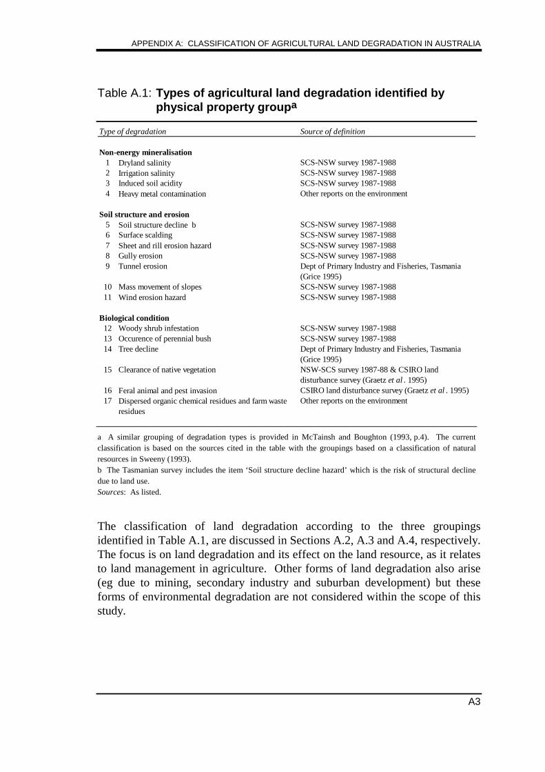
APPENDIX A: CLASSIFICATION OF AGRICULTURAL LAND DEGRADATION IN AUSTRALIA
A3
Table A.1: Types of agricultural land degradation identified byphysical property groupa
Type of degradation Source of definition
Non-energy mineralisation1 Dryland salinity SCS-NSW survey 1987-19882 Irrigation salinity SCS-NSW survey 1987-19883 Induced soil acidity SCS-NSW survey 1987-19884 Heavy metal contamination Other reports on the environment
Soil structure and erosion5 Soil structure decline b SCS-NSW survey 1987-19886 Surface scalding SCS-NSW survey 1987-19887 Sheet and rill erosion hazard SCS-NSW survey 1987-19888 Gully erosion SCS-NSW survey 1987-19889 Tunnel erosion Dept of Primary Industry and Fisheries, Tasmania
(Grice 1995)10 Mass movement of slopes SCS-NSW survey 1987-198811 Wind erosion hazard SCS-NSW survey 1987-1988
Biological condition12 Woody shrub infestation SCS-NSW survey 1987-198813 Occurence of perennial bush SCS-NSW survey 1987-198814 Tree decline Dept of Primary Industry and Fisheries, Tasmania
(Grice 1995)15 Clearance of native vegetation NSW-SCS survey 1987-88 & CSIRO land
disturbance survey (Graetz et al . 1995)16 Feral animal and pest invasion CSIRO land disturbance survey (Graetz et al . 1995)17 Dispersed organic chemical residues and farm waste
residuesOther reports on the environment
a A similar grouping of degradation types is provided in McTainsh and Boughton (1993, p.4). The currentclassification is based on the sources cited in the table with the groupings based on a classification of naturalresources in Sweeny (1993).b The Tasmanian survey includes the item ‘Soil structure decline hazard’ which is the risk of structural declinedue to land use.Sources: As listed.
The classification of land degradation according to the three groupingsidentified in Table A.1, are discussed in Sections A.2, A.3 and A.4, respectively.The focus is on land degradation and its effect on the land resource, as it relatesto land management in agriculture. Other forms of land degradation also arise(eg due to mining, secondary industry and suburban development) but theseforms of environmental degradation are not considered within the scope of thisstudy.
STAFF INFORMATION PAPER
A4
A.2 Induced changes to non-energy mineralisation
Dryland salinity (saline seepage)
Description
Dryland salinity is the build-up of salt in surface soil on non-irrigated areas usually as aresult of rising water tables and subsequent groundwater seepage. (EPA-New SouthWales 1993, p. 71)
Dryland salinity occurs on lands which are outflow zones for saline watertables. It differs from saline scalds which result from the removal of surfacesoil to expose subsoil high in salts. Once saline seepage is established, there isan increased possibility of other types of erosion (eg sheet and rill erosion andgully erosion).
Associated land use and land vulnerability
Dryland salinity can occur naturally. Anthropogenic causes come mainly fromthe clearance of native forest for agricultural and pastoral production with thefinal manifestation being dependent on local/regional geology (eg rockformations guiding underground water flows), climate (eg rainfall in rechargeareas), soil type (eg regulating the flow of water between the surface andgroundwater zones) and farm management. Clearing hillslopes of nativevegetation results in more water entering the soil due to reduced transpirationlevels of shallow rooted pastures and farm crops in comparison with the nativevegetation. Subsequently, the additional water load moves through the soil,dissolving salts which occur naturally in the soil and rock, and flowing laterallyunderground to emerge on the surface lower down the slope as salty water. Thesalt becomes concentrated in these outflow patches, as evaporation occurs,resulting in the death of all but salt-tolerant vegetation.
The bare areas so formed become subject to other types of erosion. Forexample, on grazing land, stock congregate on the sites to lick the salt. Theaccompanying trampling damages any remaining vegetation and disturbs thesurface thus aggravating the erosion problem.
Degree of severity and New South Wales base classification
The severity assessment in the New South Wales survey was based on 100hectare circles centred on sample points. If there was evidence of more thanone severity class anywhere in the area, then the whole circle was assigned tothe highest severity value observed. The severity classes and criteria areprovided in Table A.2.
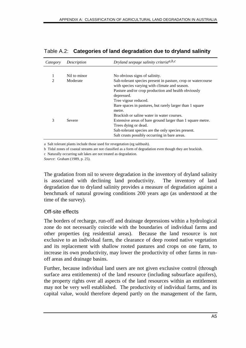
APPENDIX A: CLASSIFICATION OF AGRICULTURAL LAND DEGRADATION IN AUSTRALIA
A5
Table A.2: Categories of land degradation due to dryland salinity
Category Description Dryland seepage salinity criteriaa,b,c
1 Nil to minor No obvious signs of salinity.2 Moderate Salt-tolerant species present in pasture, crop or watercourse
with species varying with climate and season.Pasture and/or crop production and health obviouslydepressed.Tree vigour reduced.Bare spaces in pastures, but rarely larger than 1 squaremetre.Brackish or saline water in water courses.
3 Severe Extensive areas of bare ground larger than 1 square metre.Trees dying or dead.Salt-tolerant species are the only species present.Salt crusts possibly occurring in bare areas.
a Salt tolerant plants include those used for revegetation (eg saltbush).b Tidal zones of coastal streams are not classified as a form of degradation even though they are brackish.c Naturally occurring salt lakes are not treated as degradation.Source: Graham (1989, p. 25).
The gradation from nil to severe degradation in the inventory of dryland salinityis associated with declining land productivity. The inventory of landdegradation due to dryland salinity provides a measure of degradation against abenchmark of natural growing conditions 200 years ago (as understood at thetime of the survey).
Off-site effects
The borders of recharge, run-off and drainage depressions within a hydrologicalzone do not necessarily coincide with the boundaries of individual farms andother properties (eg residential areas). Because the land resource is notexclusive to an individual farm, the clearance of deep rooted native vegetationand its replacement with shallow rooted pastures and crops on one farm, toincrease its own productivity, may lower the productivity of other farms in run-off areas and drainage basins.
Further, because individual land users are not given exclusive control (throughsurface area entitlements) of the land resource (including subsurface aquifers),the property rights over all aspects of the land resources within an entitlementmay not be very well established. The productivity of individual farms, and itscapital value, would therefore depend partly on the management of the farm,
STAFF INFORMATION PAPER
A6
and partly on its proximity to common resources and the use made of thoseresources by others.
The off-site effects of dryland salinity can extend beyond the farm and localarea as the increased level of free salts on the surface may be washed intostreams and rivers. In addition, soil run-off due to secondary erosion couldenter streams and rivers. Secondary erosion could occur once dryland salinityhas reduced plant growth and increased the hazard of the soils to wind andwater erosion.
On-farm management and amelioration possibilities
Despite the fact that individual farms may not have exclusive use of the fullland resource because of the incidence of saline seepage, a number of possibletreatments come from on-farm managements practices designed to limitdegradation. For example, on-farm treatments include:
• reducing stocking rates or totally excluding stock from the effected area;
• using salt tolerant grasses, herbs, shrubs and trees on saline areas;
• surface mulching using old meadow hay or straw to facilitate moisturepenetration;
• surface tillage or deep ripping of the site to assist plant germination;
• subsurface drainage to lower the water table;
• strategic soil conservation works (eg installation of interceptor banks todivert water away from a drainage basin) to isolate affected sites fromrunoff and the risk of secondary soil erosion; and
• changes to the management of the subcatchment (as it is located on anindividual property) to incorporate high water using pastures (eg deeprooted perennial species) and regeneration of timber on groundwaterintake zones.
In a broader context, changes in management practices over a subcatchmentresource may reduce the incidence of saline seepage in individual parts of thecatchment. While a range of catchment wide and individual farm managementstrategies are available, it is important to determine which strategies orcombination of strategies, provides the greatest farm and community incomegains at least cost.

APPENDIX A: CLASSIFICATION OF AGRICULTURAL LAND DEGRADATION IN AUSTRALIA
A7
Irrigation salinity
Description
This is salting associated with irrigation land. Soils become saline when soluble saltsare concentrated in the surface horizon as a result of rising water tables. (SCS-NewSouth Wales 1989, p. 26)
The rising water levels are caused by the application of water additional to therequirements of crops and pasture. Excess water percolates to the water table,causing ground water levels to rise, thus bringing the salts into contact withvegetation. The soluble salts may come from a number of sources including:dissolved salts in the irrigation water; salt in the soil profile that is redistributedin regional groundwater systems through downward water movement; andlateral flow from an impounded source (eg channels or rice paddies) or pumpedfrom sub-artesian sources.
Associated land use and land vulnerability
Irrigation salinity occurs in areas in which irrigation farming is widespread.Areas most susceptible to salinity problems are those with underlying aquifersystems where the natural water table is relatively close to the surface and thesoil is mainly imperviable clay (eg as in the Riverina Plains of southern NewSouth Wales and north central Victoria). For areas under flood irrigation thatincorporate constructed surface bays, the risk of salinity is increased by theabsence of subsurface drainage.
Degree of severity and New South Wales base classification
As for saline seepage, the severity assessment in the New South Wales surveywas made for an 100 hectare circle centred on survey sample points. If therewas evidence of more than one severity class anywhere in the area then thewhole circle was assigned to the highest severity value observed. The severityclasses and criteria are provided in Table A.3.
Each of the categories identified in the inventory of irrigation salinity relates insome way to declining land productivity. The inventory of land degradation dueto irrigation salinity provides a measure of degradation against a benchmark ofno irrigation.
Off-site effects
Within an irrigation area, access to water tables and underground aquifersystems may not be defined by land surface entitlements. The property rights ofindividual farmers over surface areas, therefore, will not define access or

STAFF INFORMATION PAPER
A8
otherwise to subsoil resources relevant to irrigation farming. Thereforeindividual farms may not be able to fully protect themselves from the actions ofother farms working on the same or related hydrological systems.
Further, off-site effects extend outside of the local area affected by irrigationsalinity. The run-off from areas affected by irrigation salinity contain higherthan average levels of salts and other ground minerals, farm fertilisers andchemicals. The run-off lowers water quality in rivers, streams and undergroundwater reserves. The utility of the affected water is reduced for downstreamagricultural use, other industries and household consumption.
Table A.3: Categories of land degradation due to irrigation salinity
Category Description Irrigation salinity criteriaa
1 Nil to minor No obvious signs of salinity.The saline water table is greater than 5 metres from thesurface.
2 Moderate Salt-tolerant species present in pasture, crop or watercoursewith species varying with climate and season.Pasture and/or crop production and health obviouslydepressed.Tree vigour reduced.Bare spaces in pastures, but rarely larger than 1 squaremetre.Brackish or saline water in water courses (includingrevegetated areas).
3 Severe Extensive areas of bare ground larger than 1 square metre.Trees dying or dead.Salt-tolerant species are the only species present.Salt crusts possibly occurring in bare areas.Includes saline lakes that may have encrusted salt on theshore.Watertable above the surface or fluctuates and is within theroot zone of plants (ie less than 2 metres).
a Salt tolerant plants include those used for revegetation (eg saltbush).Source: Graham (1989, p. 27).
On-farm management and amelioration possibilities
The basic treatment for irrigation salinity is through the lowering of water tablesbelow the root zones of pastures and crops. This may be achieved in a numberof ways including: changes in irrigation practice so that only enough water forthe needs of crops and pasture is applied; substitution in favour of crops and
APPENDIX A: CLASSIFICATION OF AGRICULTURAL LAND DEGRADATION IN AUSTRALIA
A9
pastures needing less irrigation water; and surface management (eg deepdrainage channels). The later method may not be very effective in containingand controlling water tables in the most affected districts as water in saturatedareas will tend to seep to unsaturated areas.
Where water tables are already high and are restricting production, mechanicalsystems can be installed/used to divert saline waters and lower water levels.This process could have negative off-site effects if the drained water is allowedto enter unfiltered into the stream and river system. To counter such adverseoff-site effects, saline water may be diverted to evaporative basins (eg throughsalt interception schemes). These systems might be implemented at the farm orregional level.
Induced soil acidity
Description
Soil acidity is a process or set of processes whereby the level of hydrogen ions orcertain toxic elements increases when compared to the pristine land condition. (SCS-New South Wales 1989, p. 29)
This definition is concerned with induced (or additional) acidity, rather than theabsolute level of acidity. The New South Wales land degradation surveyadopted the induced acidity approach, while some soil studies look at the totallevel of soil acidity whether naturally occurring or induced (eg Land and WaterResources RDC 1995). From the point of view of this study, it is acidityinduced by human use that is relevant.
Associated land use and land vulnerability
Many soils are naturally acidic. Other soils may become acidic by the use ofacidifying nitrogen fertilisers; the use of legume dominated pastures which fixhigh levels of nitrogen in excess of pasture requirements; the nitrification of soilorganic compounds and their subsequent leaching from the root zone; theremoval of alkaline products and waste (eg manure); and increased soil organicmatter.
Induced soil acidity affects the chemistry of the soil which in turn affects landproductivity as the relative level of soil nutrients and their availability to plantsvaries with soil pH levels. Problem acid soils are often characterised by a pH ofless than five (measured in a calcium chloride solution). The effects of acidsoils include the release of elements that are detrimental to pasture and cropgrowth. For example, levels of aluminium or manganese increase when the pH
STAFF INFORMATION PAPER
A10
level falls below five. The resulting decreased ground cover increases thesusceptibility of the land to other forms of soil erosion.
Degree of severity and New South Wales base classification
In order to estimate induced soil acidity in the New South Wales survey, a fourhectare quadrant around each sample point was assessed. If more than oneseverity class occurred within the quadrant, then the most severe class wasrecorded. The assessment was a function of local specialist knowledge of soilpH in farm paddocks compared with undisturbed areas, soil buffer capacity(high buffer capacity soils being more resistant to pH decline than lower buffercapacity soils) and the presence of toxic elements (particularly exchangeablealuminium).
The severity of induced soil acidity in New South Wales was divided into threeclasses (see Table A.4).
The categories identified in the inventory of soil acidity relate either to apotential induced acidity problem (Categories 1 and 2) or to severe acidity(Category 3). The inventory of land degradation due to induced acidity providesa measure of degradation against a benchmark of natural conditions in thelocality of the survey point. The overall assessment is productivity based sinceproblem acid conditions are defined in terms of their potential to restrict plantgrowth and farm output potential.
Off-site effects
The off-farm effects that could occur as an indirect consequence of inducedacidification potentially include:
• dissolved organic carbon from soil acids moving into streams and reducingwater quality;
• potential risk of heavy metal contamination or low product quality; and
• reduced plant growth and water use in upper parts of the landscape whereacidification is often severe, increasing the flow of water to the water tablethus increasing dryland salinity in run-off areas and drainage basins.(Hamblin and Williams 1995).
Incidental run-off from individual farms could not be easily excluded fromsurrounding environmental amenities such as streams and rivers.
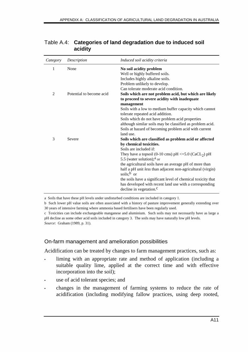
APPENDIX A: CLASSIFICATION OF AGRICULTURAL LAND DEGRADATION IN AUSTRALIA
A11
Table A.4: Categories of land degradation due to induced soilacidity
Category Description Induced soil acidity criteria
1 None No soil acidity problemWell or highly buffered soils.Includes highly alkaline soils.Problem unlikely to develop.Can tolerate moderate acid condition.
2 Potential to become acid Soils which are not problem acid, but which are likelyto proceed to severe acidity with inadequatemanagementSoils with a low to medium buffer capacity which cannottolerate repeated acid addition.Soils which do not have problem acid propertiesalthough similar soils may be classified as problem acid.Soils at hazard of becoming problem acid with currentland use.
3 Severe Soils which are classified as problem acid or affectedby chemical toxicities.Soils are included if:They have a topsoil (0-10 cms) pH <=5.0 (CaCL2) pH5.5 (water solution);a orthe agricultural soils have an average pH of more thanhalf a pH unit less than adjacent non-agricultural (virgin)soils;b orthe soils have a significant level of chemical toxicity thathas developed with recent land use with a correspondingdecline in vegetation.c
a Soils that have these pH levels under undisturbed conditions are included in category 1.b Such lower pH value soils are often associated with a history of pasture improvement generally extending over30 years of intensive farming where ammonia based fertilisers have been regularly used.c Toxicities can include exchangeable manganese and aluminium. Such soils may not necessarily have as large apH decline as some other acid soils included in category 3. The soils may have naturally low pH levels.Source: Graham (1989, p. 31).
On-farm management and amelioration possibilities
Acidification can be treated by changes to farm management practices, such as:
• liming with an appropriate rate and method of application (including asuitable quality lime, applied at the correct time and with effectiveincorporation into the soil);
• use of acid tolerant species; and
• changes in the management of farming systems to reduce the rate ofacidification (including modifying fallow practices, using deep rooted,
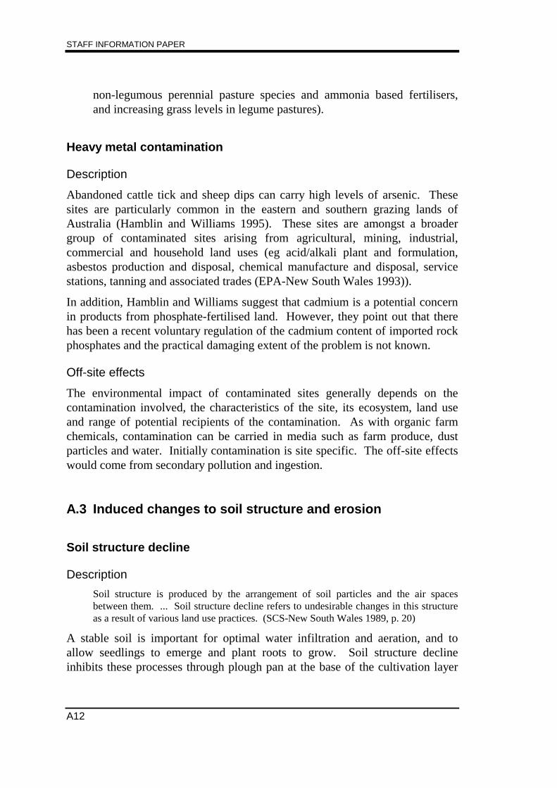
STAFF INFORMATION PAPER
A12
non-legumous perennial pasture species and ammonia based fertilisers,and increasing grass levels in legume pastures).
Heavy metal contamination
Description
Abandoned cattle tick and sheep dips can carry high levels of arsenic. Thesesites are particularly common in the eastern and southern grazing lands ofAustralia (Hamblin and Williams 1995). These sites are amongst a broadergroup of contaminated sites arising from agricultural, mining, industrial,commercial and household land uses (eg acid/alkali plant and formulation,asbestos production and disposal, chemical manufacture and disposal, servicestations, tanning and associated trades (EPA-New South Wales 1993)).
In addition, Hamblin and Williams suggest that cadmium is a potential concernin products from phosphate-fertilised land. However, they point out that therehas been a recent voluntary regulation of the cadmium content of imported rockphosphates and the practical damaging extent of the problem is not known.
Off-site effects
The environmental impact of contaminated sites generally depends on thecontamination involved, the characteristics of the site, its ecosystem, land useand range of potential recipients of the contamination. As with organic farmchemicals, contamination can be carried in media such as farm produce, dustparticles and water. Initially contamination is site specific. The off-site effectswould come from secondary pollution and ingestion.
A.3 Induced changes to soil structure and erosion
Soil structure decline
Description
Soil structure is produced by the arrangement of soil particles and the air spacesbetween them. ... Soil structure decline refers to undesirable changes in this structureas a result of various land use practices. (SCS-New South Wales 1989, p. 20)
A stable soil is important for optimal water infiltration and aeration, and toallow seedlings to emerge and plant roots to grow. Soil structure declineinhibits these processes through plough pan at the base of the cultivation layer

APPENDIX A: CLASSIFICATION OF AGRICULTURAL LAND DEGRADATION IN AUSTRALIA
A13
and compression. A stable soil structure also reduces susceptibility of soil toother types of degradation.
Associated land use and land vulnerability
The most substantial changes can be attributed to cropping practices. Tillagemachinery can pulverise the soil aggregates and generally compact the soil.Eventually, a very dense layer (referred to as ‘plough pan’) forms at the base ofthe cultivation layer. The amount of soil organic matter, part of soil structureand fertility, is also reduced by tillage.
Trampling by stock also causes a decline in soil structure, but this effect isgenerally less severe than effects arising from the use of cultivation machinery.
Different soil groups differ in susceptibility to structural decline. Fine sands,silts and medium sands have little structure to begin with and therefore theirstructure would change little with farming. Coarse sands, loams andsandy/loamy soils (eg light textured brown soils, skeletal soils and red brownearths), and clays and clay loams are more structured and therefore can bedegraded structurally in the short term. With appropriate management, structurecan be re-established in the longer term.
Degree of severity and New South Wales base classification
In order to estimate the severity of soil structure decline in the New SouthWales survey, a four hectare quadrant around each sample point was assessed.If more than one severity class occurred within the quadrant, then the mostsevere class was recorded. The severity of structural decline at each samplepoint was determined by considering the land use, cultivation history andintensity (with an initial assumption that the longer an area had been cropped,the greater the cultivation cycles and the greater the degree of degradation),evidence of hardpans, surface crusts, vulnerability of local soil types tostructural decline, land use rotations and local knowledge. Assessments weremade in comparison to benchmark undisturbed sites in the vicinity of eachsurvey point. The degree of soil structure decline was recorded according to thefollowing regime (see Table A.5).
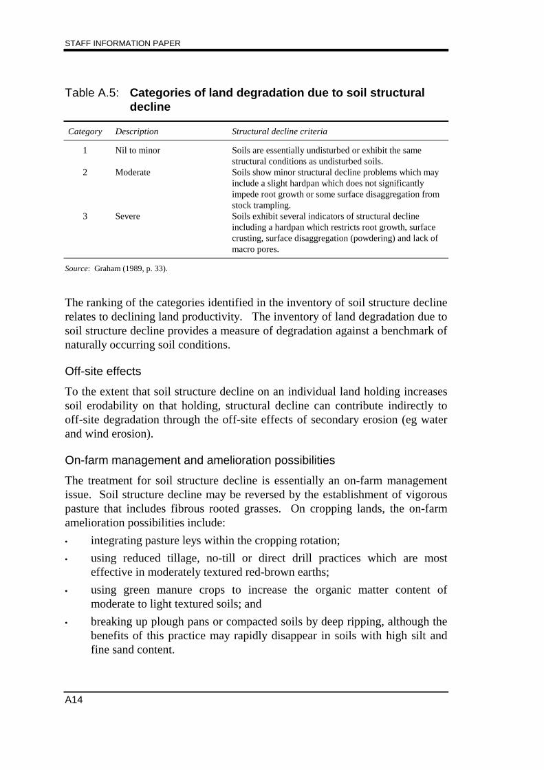
STAFF INFORMATION PAPER
A14
Table A.5: Categories of land degradation due to soil structuraldecline
Category Description Structural decline criteria
1 Nil to minor Soils are essentially undisturbed or exhibit the samestructural conditions as undisturbed soils.
2 Moderate Soils show minor structural decline problems which mayinclude a slight hardpan which does not significantlyimpede root growth or some surface disaggregation fromstock trampling.
3 Severe Soils exhibit several indicators of structural declineincluding a hardpan which restricts root growth, surfacecrusting, surface disaggregation (powdering) and lack ofmacro pores.
Source: Graham (1989, p. 33).
The ranking of the categories identified in the inventory of soil structure declinerelates to declining land productivity. The inventory of land degradation due tosoil structure decline provides a measure of degradation against a benchmark ofnaturally occurring soil conditions.
Off-site effects
To the extent that soil structure decline on an individual land holding increasessoil erodability on that holding, structural decline can contribute indirectly tooff-site degradation through the off-site effects of secondary erosion (eg waterand wind erosion).
On-farm management and amelioration possibilities
The treatment for soil structure decline is essentially an on-farm managementissue. Soil structure decline may be reversed by the establishment of vigorouspasture that includes fibrous rooted grasses. On cropping lands, the on-farmamelioration possibilities include:
• integrating pasture leys within the cropping rotation;
• using reduced tillage, no-till or direct drill practices which are mosteffective in moderately textured red-brown earths;
• using green manure crops to increase the organic matter content ofmoderate to light textured soils; and
• breaking up plough pans or compacted soils by deep ripping, although thebenefits of this practice may rapidly disappear in soils with high silt andfine sand content.
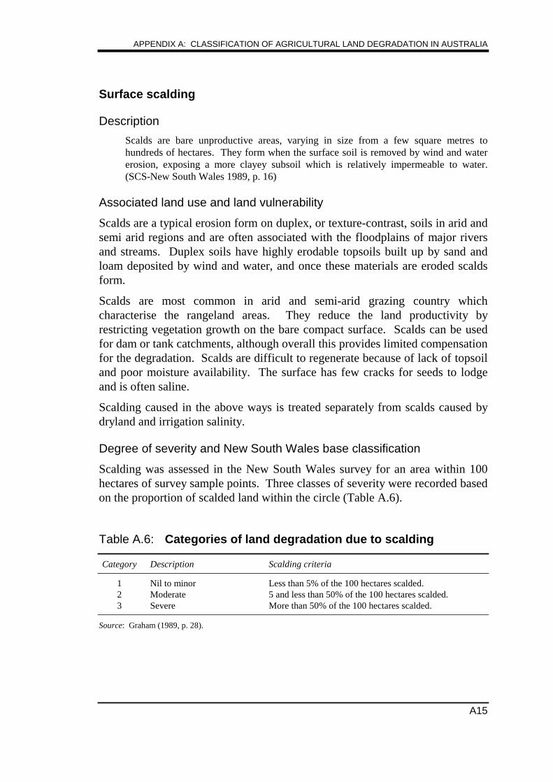
APPENDIX A: CLASSIFICATION OF AGRICULTURAL LAND DEGRADATION IN AUSTRALIA
A15
Surface scalding
Description
Scalds are bare unproductive areas, varying in size from a few square metres tohundreds of hectares. They form when the surface soil is removed by wind and watererosion, exposing a more clayey subsoil which is relatively impermeable to water.(SCS-New South Wales 1989, p. 16)
Associated land use and land vulnerability
Scalds are a typical erosion form on duplex, or texture-contrast, soils in arid andsemi arid regions and are often associated with the floodplains of major riversand streams. Duplex soils have highly erodable topsoils built up by sand andloam deposited by wind and water, and once these materials are eroded scaldsform.
Scalds are most common in arid and semi-arid grazing country whichcharacterise the rangeland areas. They reduce the land productivity byrestricting vegetation growth on the bare compact surface. Scalds can be usedfor dam or tank catchments, although overall this provides limited compensationfor the degradation. Scalds are difficult to regenerate because of lack of topsoiland poor moisture availability. The surface has few cracks for seeds to lodgeand is often saline.
Scalding caused in the above ways is treated separately from scalds caused bydryland and irrigation salinity.
Degree of severity and New South Wales base classification
Scalding was assessed in the New South Wales survey for an area within 100hectares of survey sample points. Three classes of severity were recorded basedon the proportion of scalded land within the circle (Table A.6).
Table A.6: Categories of land degradation due to scalding
Category Description Scalding criteria
1 Nil to minor Less than 5% of the 100 hectares scalded.2 Moderate 5 and less than 50% of the 100 hectares scalded.3 Severe More than 50% of the 100 hectares scalded.
Source: Graham (1989, p. 28).
STAFF INFORMATION PAPER
A16
Each of the categories identified in the inventory of scalding is determined bythe physical appearance of the land. The inventory of land degradation due toscalding provides a measure of degradation against a benchmark of no scalding.
Off-site effects
The direct effects of scalding are localised with the possibility of some erosioncreep across farm boundaries. Nevertheless, once the ground is subject toscalding there is vegetation loss and it becomes vulnerable to other forms oferosion such as wind, sheet and rill erosion. To the extent that these erosiontypes combine with scalding, the off-site effects would be similar to those forthe other erosion groups.
On-farm management and amelioration possibilities
Scalding is a localised form of land degradation and the ameliorationpossibilities are therefore also localised. Rehabilitation techniques aim atimproving the infiltration of runoff water into the scald surface, trappingwindblown seeds and providing an improved environment for seedling growth.For example, water ponds are used to reclaim scalds as they improve themoisture regime by holding runoff water on the scald surface where it can beslowly absorbed. The addition of water also reduces surface salinity and formsan uneven surface which is conducive to revegetation.
Revegetation also depends on an abundant supply of fertile seed. While annualplants establish themselves quickly, to achieve durable regeneration, it may benecessary to reintroduce perennial species such as saltbush by hand sowing orseeding.
Sheet and rill erosion
Description
Sheet and rill erosion are two of several forms of land degradation resultingfrom flowing water. They mainly occur on sloping land where there isinsufficient ground cover to prevent soil loss.
Sheet erosion involves the removal of a fairly uniform layer of soil from the landsurface by raindrop splash and/or runoff. No perceptible channels are formed. Rillerosion is the removal of soil by runoff, with numerous small channels, generally up to30 cm deep being formed. (SCS-New South Wales 1989, p. 4)
APPENDIX A: CLASSIFICATION OF AGRICULTURAL LAND DEGRADATION IN AUSTRALIA
A17
Associated land use and land vulnerability
Sheet and rill erosion are most severe on cultivated lands. Rill erosion typicallyoccurs on recently cultivated or disturbed soils. It also occurs on grasslandswhere pasture cover is minimal or when pastures are cultivated for resowing orestablishment of fodder crops. Similar problems exist in tree plantations duringstages of site preparation and planting.
Sheet and rill erosion can be most significant at the end of a drought whenvegetation cover is negligible and significant amounts of topsoil carryingorganic matter, phosphate fertiliser and reactive clay that make up the majorityof the soil’s fertility can be lost (Hamblin and Williams 1995).
The New South Wales survey considered these two erosion forms togetherbecause farm management techniques for controlling them are usually the same.
Degree of severity and New South Wales base classification
The visible effects of sheet and rill erosion can disappear soon after they occur.Therefore, the New South Wales survey assessed land degradation due to sheetand rill erosion by estimating the vulnerability of land to sheet and rill erosion.The estimated degree of vulnerability is referred to as the erosion ‘hazard’prevailing under current land use, land condition, soil type, and climate.However, the estimate of hazard does not measure the erosion that has occurredin the past, nor does it predict the erosion that could occur with a shift to highlyexploitative land management practices or climatic extremes.
Hazard is indicated using a modified form of the Universal Soil Loss Equation(USLE). The USLE adopted by SCS-New South Wales uses five factors:rainfall erosivity (R); soil erodibility (K); slope length and gradient (LS); groundcover (C); and management practices (P). Hazard was evaluated in the model:
A R K LS C P= * * * * .
The estimated rate of soil loss (A) is measured in tonnes per hectare per annum(see Table A.7).
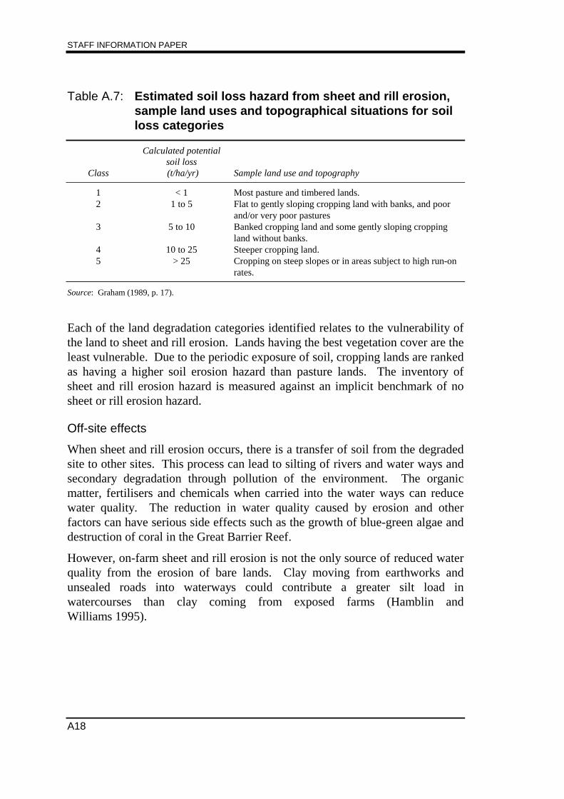
STAFF INFORMATION PAPER
A18
Table A.7: Estimated soil loss hazard from sheet and rill erosion,sample land uses and topographical situations for soilloss categories
Class
Calculated potentialsoil loss (t/ha/yr) Sample land use and topography
1 < 1 Most pasture and timbered lands.2 1 to 5 Flat to gently sloping cropping land with banks, and poor
and/or very poor pastures3 5 to 10 Banked cropping land and some gently sloping cropping
land without banks.4 10 to 25 Steeper cropping land.5 > 25 Cropping on steep slopes or in areas subject to high run-on
rates.
Source: Graham (1989, p. 17).
Each of the land degradation categories identified relates to the vulnerability ofthe land to sheet and rill erosion. Lands having the best vegetation cover are theleast vulnerable. Due to the periodic exposure of soil, cropping lands are rankedas having a higher soil erosion hazard than pasture lands. The inventory ofsheet and rill erosion hazard is measured against an implicit benchmark of nosheet or rill erosion hazard.
Off-site effects
When sheet and rill erosion occurs, there is a transfer of soil from the degradedsite to other sites. This process can lead to silting of rivers and water ways andsecondary degradation through pollution of the environment. The organicmatter, fertilisers and chemicals when carried into the water ways can reducewater quality. The reduction in water quality caused by erosion and otherfactors can have serious side effects such as the growth of blue-green algae anddestruction of coral in the Great Barrier Reef.
However, on-farm sheet and rill erosion is not the only source of reduced waterquality from the erosion of bare lands. Clay moving from earthworks andunsealed roads into waterways could contribute a greater silt load inwatercourses than clay coming from exposed farms (Hamblin andWilliams 1995).
APPENDIX A: CLASSIFICATION OF AGRICULTURAL LAND DEGRADATION IN AUSTRALIA
A19
On-farm management and amelioration possibilities
Sheet and rill erosion is largely an on-farm problem, although having occurred,run-offs of soil would affect other farms and increase sediments in riversystems.
Management and treatment involve maintaining a good ground cover of grasses,herbs or leaf litter. On cultivated lands soil conservation and structural workssuch as contour banks can be used to reduce the velocity of surface run-off,divert run-off to safe disposal sites, and contain sediment within channel banks.Tillage on natural contours can also prevent sheet and rill erosion.
Crop and soil management practices that reduce on-farm sheet and rill erosionon cultivated land include: changes to rotations to reduce the number ofcultivations; stubble retention to protect the ground surface; green manuring toimprove organic matter levels; and reduced or non-tillage systems whichinvolve the use of non-residual herbicides to control weed growth and reducethe level of soil disturbance (although the use of additional chemicals may haveits own adverse effects).
On grazing lands, ground cover can be improved by adjusting stocking rates andremoving stock when ground cover falls below critical limits, evenlydistributing grazing points and applying fertilisers, including trace elements forknown deficiencies. If erosion levels are severe, constructing works to controlsurface runoff across bare areas and assist revegetation can be used for soilconservation.
Gully erosion
Description
A gully is an open incised erosion channel down which water flows during orimmediately after rain.
Gullies are generally deeper than 30 cms. Any erosion channel less than this depth isclassified as rill as it can usually be removed by tillage. Areas of stream bank erosionare included in the assessment of gully erosion. (SCS-New South Wales 1989, p. 6)
The major effects of gully erosion are the removal of fertile topsoil layers,sedimentation of creeks, rivers and water supplies, and the formation ofpathways for the removal of sediments from adjacent areas.
Associated land use and land vulnerability
Gully erosion occurs when small rill streams unite to create a stronger flow. Itis evident in cropping and grazing country under similar conditions to sheet and
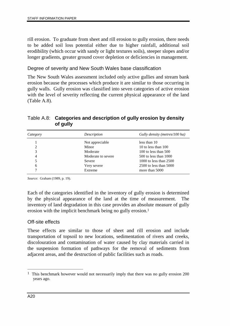
STAFF INFORMATION PAPER
A20
rill erosion. To graduate from sheet and rill erosion to gully erosion, there needsto be added soil loss potential either due to higher rainfall, additional soilerodibility (which occur with sandy or light textures soils), steeper slopes and/orlonger gradients, greater ground cover depletion or deficiencies in management.
Degree of severity and New South Wales base classification
The New South Wales assessment included only active gullies and stream bankerosion because the processes which produce it are similar to those occurring ingully walls. Gully erosion was classified into seven categories of active erosionwith the level of severity reflecting the current physical appearance of the land(Table A.8).
Table A.8: Categories and description of gully erosion by densityof gully
Category Description Gully density (metres/100 ha)
1 Not appreciable less than 102 Minor 10 to less than 1003 Moderate 100 to less than 5004 Moderate to severe 500 to less than 10005 Severe 1000 to less than 25006 Very severe 2500 to less than 50007 Extreme more than 5000
Source: Graham (1989, p. 19).
Each of the categories identified in the inventory of gully erosion is determinedby the physical appearance of the land at the time of measurement. Theinventory of land degradation in this case provides an absolute measure of gullyerosion with the implicit benchmark being no gully erosion.1
Off-site effects
These effects are similar to those of sheet and rill erosion and includetransportation of topsoil to new locations, sedimentation of rivers and creeks,discolouration and contamination of water caused by clay materials carried inthe suspension formation of pathways for the removal of sediments fromadjacent areas, and the destruction of public facilities such as roads.
1 This benchmark however would not necessarily imply that there was no gully erosion 200
years ago.
APPENDIX A: CLASSIFICATION OF AGRICULTURAL LAND DEGRADATION IN AUSTRALIA
A21
On-farm management and amelioration possibilities
On-farm effects include: the removal of the more fertile top layers of soil;lowering of the water table which can adversely affect plants in adjacent areas(in contrast to salinity where the presence of a rising water table is the problem);reduction of the area of arable land; the division of land into smaller parcelsincreasing the costs of farming operations; and damage to farm improvements(such as fences traversing erosion gullies).
Gully erosion is linearly concentrated in comparison to sheet and rill erosionand while gully erosion is restricted to areas with a concentration of waterflows, such areas would not necessarily be confined to individual holdings.Therefore, without containment strategies on a degraded holding or an adjoiningholding sharing the same drainage channels, the erosion would spread betweenproperties.
A number of on-farm management practices are available for treating gullyerosion. These treatments may include soil conservation earthworks and theadoption of management practices that better match the capability of the land.Changing management practices can involve changes in land use. For example,eroded cropping land can be rested by converting it to fallow land, grazing landor possibly allowing the return of native forest. Grazing land may be used lessintensively or withdrawn from production to allow reafforestation to take place.
Tunnel erosion
Description
Tunnel erosion is:
... the transportation of sub-surface soil by water while the surface remains relativelyintact. It relies on the seepage of water into dry soil causing dispersion of soil particlesinto suspension. The dispersed soil is then removed by seepage until the seepage pathgradually enlarges to a tunnel. (Grice 1995, p. 32)
The transported material emerges through a gully wall, an embankment, or isforced to the surface through hydrostatic pressure. Tunnels enlarge during wetperiods and eventually collapse in the normal course of events to form gullies orpotholes.
Associated land use and land vulnerability
In Tasmania, tunnel erosion is largely confined to the south of the state in areasdominated by Permian mudstone and Triassic sandstone. The tunnels form in

STAFF INFORMATION PAPER
A22
complex parent rocks with interbedded sequences or with rapid internaldrainage, depending on the nature of local subsurface systems.
The major problem identified with tunnel erosion is the hazard to livestock andtraffic plus the tendency for tunnels to form gullies.
Degree of severity in Tasmanian base classification
Tunnel erosion was assessed by inspection of the extent of erosion in a typical100 hectare zone of a land system or its component. Tunnel erosion wasclassified into three categories of severity reflecting the incidence of this formof degradation (Table A.9)
Table A.9: Categories and description of tunnel erosion by densityof tunnel
Category Description Tunnel density
1 None No evident tunnel erosion.2 Minor Tunnels present were less than
one metre in depth from groundsurface to tunnel floor.
3 Severe Tunnel depth exceeds onemetre.
Source: Grice (1995, p. 32).
Off-site effects
These would be similar to gully erosion involving transportation of soil to newlocations, sedimentation of rivers and creeks, discolouration and contaminationof water, and the destruction of facilities undermined by tunnels.
Mass movement
Description
Mass movement is a process that involves the downward movement of soil and rockmaterials under the influence of gravity. (SCS-New South Wales 1989, p. 8)
The process is complex and the movement of material may be continual,episodic or catastrophic. There are many forms of mass movement includingsoil creep, earthflow, slumps, land slips, landslides and rock avalanches.
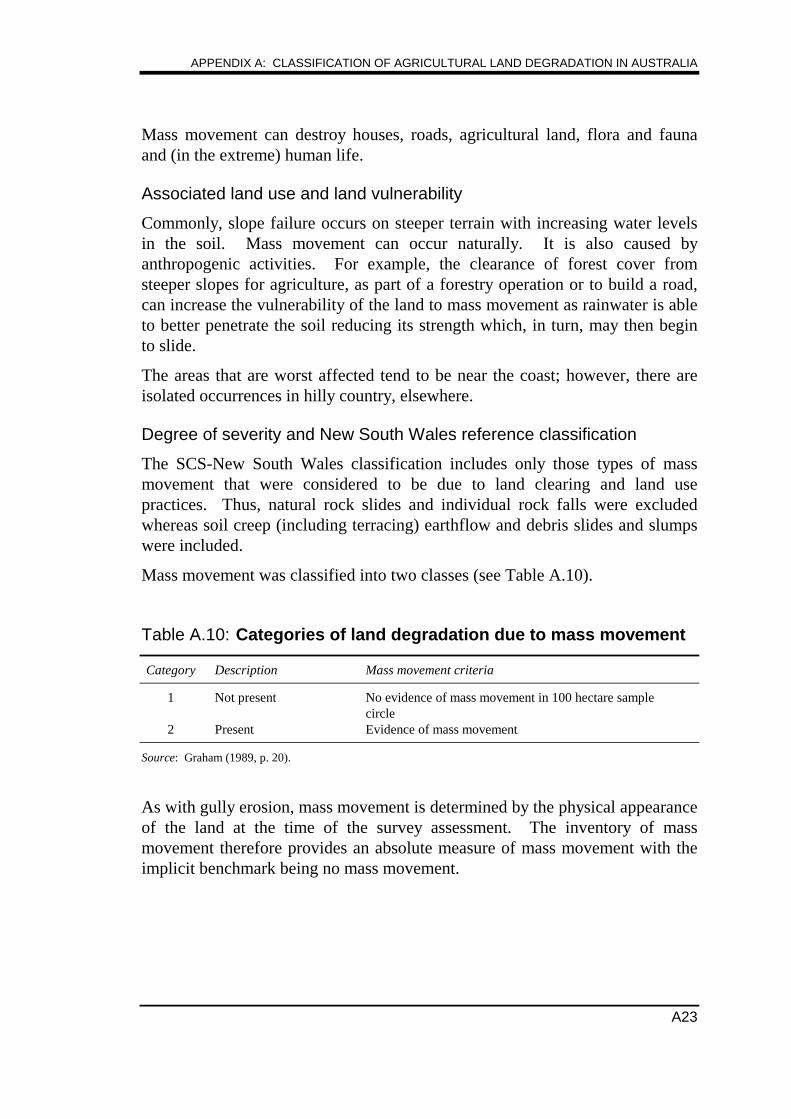
APPENDIX A: CLASSIFICATION OF AGRICULTURAL LAND DEGRADATION IN AUSTRALIA
A23
Mass movement can destroy houses, roads, agricultural land, flora and faunaand (in the extreme) human life.
Associated land use and land vulnerability
Commonly, slope failure occurs on steeper terrain with increasing water levelsin the soil. Mass movement can occur naturally. It is also caused byanthropogenic activities. For example, the clearance of forest cover fromsteeper slopes for agriculture, as part of a forestry operation or to build a road,can increase the vulnerability of the land to mass movement as rainwater is ableto better penetrate the soil reducing its strength which, in turn, may then beginto slide.
The areas that are worst affected tend to be near the coast; however, there areisolated occurrences in hilly country, elsewhere.
Degree of severity and New South Wales reference classification
The SCS-New South Wales classification includes only those types of massmovement that were considered to be due to land clearing and land usepractices. Thus, natural rock slides and individual rock falls were excludedwhereas soil creep (including terracing) earthflow and debris slides and slumpswere included.
Mass movement was classified into two classes (see Table A.10).
Table A.10: Categories of land degradation due to mass movement
Category Description Mass movement criteria
1 Not present No evidence of mass movement in 100 hectare samplecircle
2 Present Evidence of mass movement
Source: Graham (1989, p. 20).
As with gully erosion, mass movement is determined by the physical appearanceof the land at the time of the survey assessment. The inventory of massmovement therefore provides an absolute measure of mass movement with theimplicit benchmark being no mass movement.
STAFF INFORMATION PAPER
A24
Off-site effects
Quite clearly most of the effects relating to mass movement would beconcentrated at the movement site. Off-site effects would be similar to sheet rilland gully erosion including siltation of water ways.
On-farm management and amelioration possibilities
Land damage by mass movement could be expensive to repair and may removedamaged land from agricultural production. In highly unstable lands, theappropriate farm management strategy may be to limit the use of unstable lands,reduce clearing of slopes or adopt engineering approaches such as decreasingslope angles and reducing water levels in the soil.2
Wind erosion
Description
Wind erosion is the detachment and transportation of soil by wind. (SCS-New SouthWales 1989, p. 10)
Extreme examples of wind erosion are the Mallee dust storms of the 1930s, andmore recently, those associated with the droughts of 1982–83 and 1994–95.Unlike water erosion, wind can erode upslope with the angle of air flowchanging quickly. Eroded soil can be transported a great distance.
Associated land use and land vulnerability
Sandy soils in drier areas can be blown away if they are not protected by plantcover and are therefore the most vulnerable. Soil vulnerability is increased byrepeated disturbance of a surface by tillage or grazing stock. The disturbancehas the effect of pulverising soil aggregates (eg into dust) making the soil evenmore susceptible to wind erosion. Vulnerability is further increased by the lossof the finer soil particles which cause a reduction in the soil’s nutrient levels andits ability to retain moisture for plant growth.
Degree of severity and New South Wales base classification
As with sheet and rill erosion, the degree of degradation from wind erosion isassessed by a wind erosion hazard rating. This rating describes the relative
2 Engineering solutions to contain potential mass movement in unstable areas, in general may
be more evident along roadways or in areas subject to residential or other development,than in rural areas because of the greater cost/inconvenience of mass movement in thoseareas.
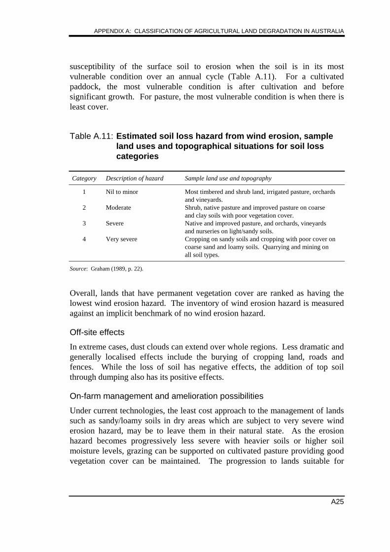
APPENDIX A: CLASSIFICATION OF AGRICULTURAL LAND DEGRADATION IN AUSTRALIA
A25
susceptibility of the surface soil to erosion when the soil is in its mostvulnerable condition over an annual cycle (Table A.11). For a cultivatedpaddock, the most vulnerable condition is after cultivation and beforesignificant growth. For pasture, the most vulnerable condition is when there isleast cover.
Table A.11: Estimated soil loss hazard from wind erosion, sampleland uses and topographical situations for soil losscategories
Category Description of hazard Sample land use and topography
1 Nil to minor Most timbered and shrub land, irrigated pasture, orchardsand vineyards.
2 Moderate Shrub, native pasture and improved pasture on coarseand clay soils with poor vegetation cover.
3 Severe Native and improved pasture, and orchards, vineyardsand nurseries on light/sandy soils.
4 Very severe Cropping on sandy soils and cropping with poor cover oncoarse sand and loamy soils. Quarrying and mining onall soil types.
Source: Graham (1989, p. 22).
Overall, lands that have permanent vegetation cover are ranked as having thelowest wind erosion hazard. The inventory of wind erosion hazard is measuredagainst an implicit benchmark of no wind erosion hazard.
Off-site effects
In extreme cases, dust clouds can extend over whole regions. Less dramatic andgenerally localised effects include the burying of cropping land, roads andfences. While the loss of soil has negative effects, the addition of top soilthrough dumping also has its positive effects.
On-farm management and amelioration possibilities
Under current technologies, the least cost approach to the management of landssuch as sandy/loamy soils in dry areas which are subject to very severe winderosion hazard, may be to leave them in their natural state. As the erosionhazard becomes progressively less severe with heavier soils or higher soilmoisture levels, grazing can be supported on cultivated pasture providing goodvegetation cover can be maintained. The progression to lands suitable for

STAFF INFORMATION PAPER
A26
cropping is more gradual, with some drier, sandy/loamy areas suitable forcultivation for grazing but not suited to cultivation for annual crops.
Land characterised by heavier soils or soils with higher moisture content havelower wind erosion hazard when cropped. On cropping lands, the wind erosionhazard can be reduced through: the retention of crop stubble for as long aspossible after harvest; avoidance of stubble burning; sowing seeds into stubbleresidues; and reduced tillage. In addition, increasing lengths of pasture rotationbetween crops can be used to improve soil structure and reduce wind erosionhazard.
As with sheet and rill erosion, wind erosion is an extensive form of surfacedegradation which could spread between holdings within a locality at risk.Without containment strategies by holdings, the incidence of wind erosion couldspread.
A.4 Induced changes to biological conditions
There are a number of degradation types which were not included in the NewSouth Wales survey of land degradation but which appear to reduce farmproductivity and the utility of the environment as a natural asset. With theexception of woody shrub infestation and perennial bush decline which wereincluded in the New South Wales survey, these forms of agricultural landdegradation include clearance of native vegetation, tree decline, feral and otheranimal invasion, and dispersed organic chemical residues and farm wasteresidues.
Woody shrub infestation
Description
Woody shrubs (woody weeds) are inedible native plants that are rapidly infesting largeareas of semi arid to arid regions. (SCS-New South Wales 1989, p. 8)
Growing up to 3 metres in height, woody shrubs commonly occur as densestands, although they may appear as individual bushes or small clumps. Speciesof native inedible woody shrub in New South Wales include:
• turpentine (Eremophila sturtii);
• budda (Eremophila mitchelli);
• narrowleaf hopbush (Dodonea viscosa ssp. angustissima);
• broadleaf hopbush (Dodonea viscosa ssp. angustifolia);
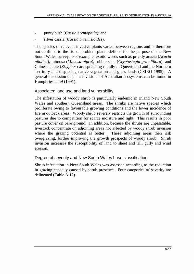
APPENDIX A: CLASSIFICATION OF AGRICULTURAL LAND DEGRADATION IN AUSTRALIA
A27
• punty bush (Cassia eremophila); and
• silver cassia (Cassia artemisioides).
The species of relevant invasive plants varies between regions and is thereforenot confined to the list of problem plants defined for the purpose of the NewSouth Wales survey. For example, exotic weeds such as prickly acacia (Acacianilotica), mimosa (Mimosa pigra), rubber vine (Cryptostegia grandiflora), andChinese apple (Zizyphus) are spreading rapidly in Queensland and the NorthernTerritory and displacing native vegetation and grass lands (CSIRO 1995). Ageneral discussion of plant invasions of Australian ecosystems can be found inHumphries et. al (1991).
Associated land use and land vulnerability
The infestation of woody shrub is particularly endemic in inland New SouthWales and southern Queensland areas. The shrubs are native species whichproliferate owing to favourable growing conditions and the lower incidence offire in outback areas. Woody shrub severely restricts the growth of surroundingpastures due to competition for scarce moisture and light. This results in poorpasture cover on bare ground. In addition, because the shrubs are unpalatable,livestock concentrate on adjoining areas not affected by woody shrub invasionwhere the grazing potential is better. These adjoining areas then riskovergrazing, further improving the growth prospects of woody shrub. Shrubinvasion increases the susceptibility of land to sheet and rill, gully and winderosion.
Degree of severity and New South Wales base classification
Shrub infestation in New South Wales was assessed according to the reductionin grazing capacity caused by shrub presence. Four categories of severity aredelineated (Table A.12).
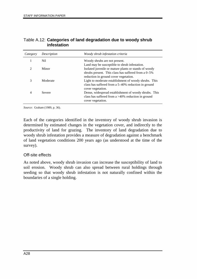
STAFF INFORMATION PAPER
A28
Table A.12: Categories of land degradation due to woody shrubinfestation
Category Description Woody shrub infestation criteria
1 Nil Woody shrubs are not present.Land may be susceptible to shrub infestation.
2 Minor Isolated juvenile or mature plants or stands of woodyshrubs present. This class has suffered from a 0–5%reduction in ground cover vegetation.
3 Moderate Light to moderate establishment of woody shrubs. Thisclass has suffered from a 5–40% reduction in groundcover vegetation.
4 Severe Dense, widespread establishment of woody shrubs. Thisclass has suffered from a >40% reduction in groundcover vegetation.
Source: Graham (1989, p. 36).
Each of the categories identified in the inventory of woody shrub invasion isdetermined by estimated changes in the vegetation cover, and indirectly to theproductivity of land for grazing. The inventory of land degradation due towoody shrub infestation provides a measure of degradation against a benchmarkof land vegetation conditions 200 years ago (as understood at the time of thesurvey).
Off-site effects
As noted above, woody shrub invasion can increase the susceptibility of land tosoil erosion. Woody shrub can also spread between rural holdings throughseeding so that woody shrub infestation is not naturally confined within theboundaries of a single holding.

APPENDIX A: CLASSIFICATION OF AGRICULTURAL LAND DEGRADATION IN AUSTRALIA
A29
On-farm management and amelioration possibilities
The localised nature of woody shrub infestation is essentially determined by theinvasiveness of the weed plant. The relevant solutions begin at the farm level,but could extend beyond individual farms where the weed invasion has gonebeyond the control of individual farmers or it has invaded non-farm land, suchas road sides, reserves and residential areas. Treatments for woody weedinclude:
• prescribed burning which is effective against young and scattered woodyshrubs;
• mechanical control including pushing, chaining, and root ploughing or theuse of land imprinting rollers (or ‘sheep foot’ rollers);
• chemical control by point application for selective treatment; and
• cropping, which is limited to areas of reliable rainfall.
Perennial bush decline
Description
The death of edible perennial bush is a significant form of land degradation in the semi-arid and arid regions of New South Wales. Good perennial bush cover providesprotection of the soil surface from wind erosion, creates more favourable groundsurface conditions for pasture plants and provides an important source of stock fodderduring droughts. (SCS-New South Wales 1989, p. 28)
Associated land use and land vulnerability
Overgrazing of perennial bush can reduce its occurrence or eliminate it. Forexample, in adjoining grazing areas, perennial bush might be seen on one sideof a boundary fence and not on the other as a result of different grazingmanagement practices on either side of the fence.
Historically, perennial bush has not been evenly distributed throughout the semiarid and arid regions. The actual distribution depends on climate, soils andlandforms. As there is no benchmark against which to assess the degree ofdegradation, the New South Wales survey mapped the presence and relativedensity of perennial bush in the State. The species for which incidence wassurveyed included:
• bladder saltbush (Atriplex vesicaria);
• black blue bush (Maireana pyramidata); and
• pearl blue bush (Maireana sedifolia).
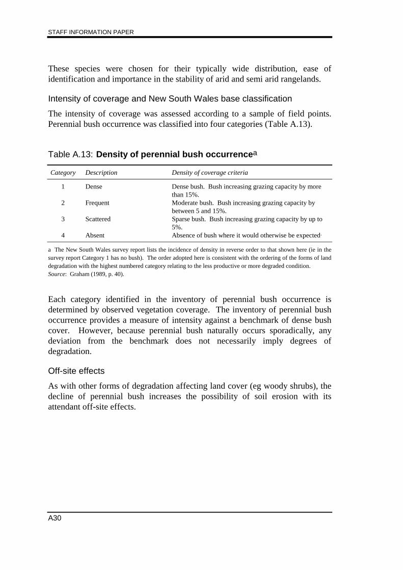
STAFF INFORMATION PAPER
A30
These species were chosen for their typically wide distribution, ease ofidentification and importance in the stability of arid and semi arid rangelands.
Intensity of coverage and New South Wales base classification
The intensity of coverage was assessed according to a sample of field points.Perennial bush occurrence was classified into four categories (Table A.13).
Table A.13: Density of perennial bush occurrencea
Category Description Density of coverage criteria
1 Dense Dense bush. Bush increasing grazing capacity by morethan 15%.
2 Frequent Moderate bush. Bush increasing grazing capacity bybetween 5 and 15%.
3 Scattered Sparse bush. Bush increasing grazing capacity by up to5%.
4 Absent Absence of bush where it would otherwise be expected.
a The New South Wales survey report lists the incidence of density in reverse order to that shown here (ie in thesurvey report Category 1 has no bush). The order adopted here is consistent with the ordering of the forms of landdegradation with the highest numbered category relating to the less productive or more degraded condition.Source: Graham (1989, p. 40).
Each category identified in the inventory of perennial bush occurrence isdetermined by observed vegetation coverage. The inventory of perennial bushoccurrence provides a measure of intensity against a benchmark of dense bushcover. However, because perennial bush naturally occurs sporadically, anydeviation from the benchmark does not necessarily imply degrees ofdegradation.
Off-site effects
As with other forms of degradation affecting land cover (eg woody shrubs), thedecline of perennial bush increases the possibility of soil erosion with itsattendant off-site effects.

APPENDIX A: CLASSIFICATION OF AGRICULTURAL LAND DEGRADATION IN AUSTRALIA
A31
On-farm management and amelioration possibilities
Perennial bush decline is essentially a local problem with the possibletreatments including:
• reseeding of overgrazed areas;
• grazing management strategies to reduce stock concentrations at criticaltimes during the flowering, seeding and seedling establishment phases ofthe plant cycle; and
• excluding stock when bushes are being overgrazed.
Tree decline
Description
Tree decline:
... is the sudden or gradual death of trees (Grice 1995, p. 33).
Associated land use and land vulnerability
In Tasmania (the state which provides the reference for this category), treedecline particularly effects eucalypts on drier areas of agricultural land. TheTasmania study points out that the Phytophthora cinnamomi root rot funguswhich causes dieback of Jarrah in Western Australia is not implicated in the treedecline of agricultural land in Tasmania.
In Tasmania, factors implicated in tree decline include: drought; repeateddefoliation by possums or insects; damage to root systems by cultivation orcompaction by livestock; and changes in the micro climate as surrounding treesare removed. In addition, grazing of seedlings or coppice results in lack ofregeneration and the eventual death of mature stands due to old age. Overall,tree decline was found in Tasmania to be more typical of the lower rainfallareas.
Degree of severity and Tasmanian base classification
The Tasmanian methodology assessed degradation using land systems as‘sample points’. This was deemed appropriate because of the small size of thestate and the complexity of land forms. The vigour of the majority of trees in aland system was assessed by survey field officers and classified according to thefollowing classes of severity (Table A.14). The implicit benchmark for thesurvey is healthy trees.
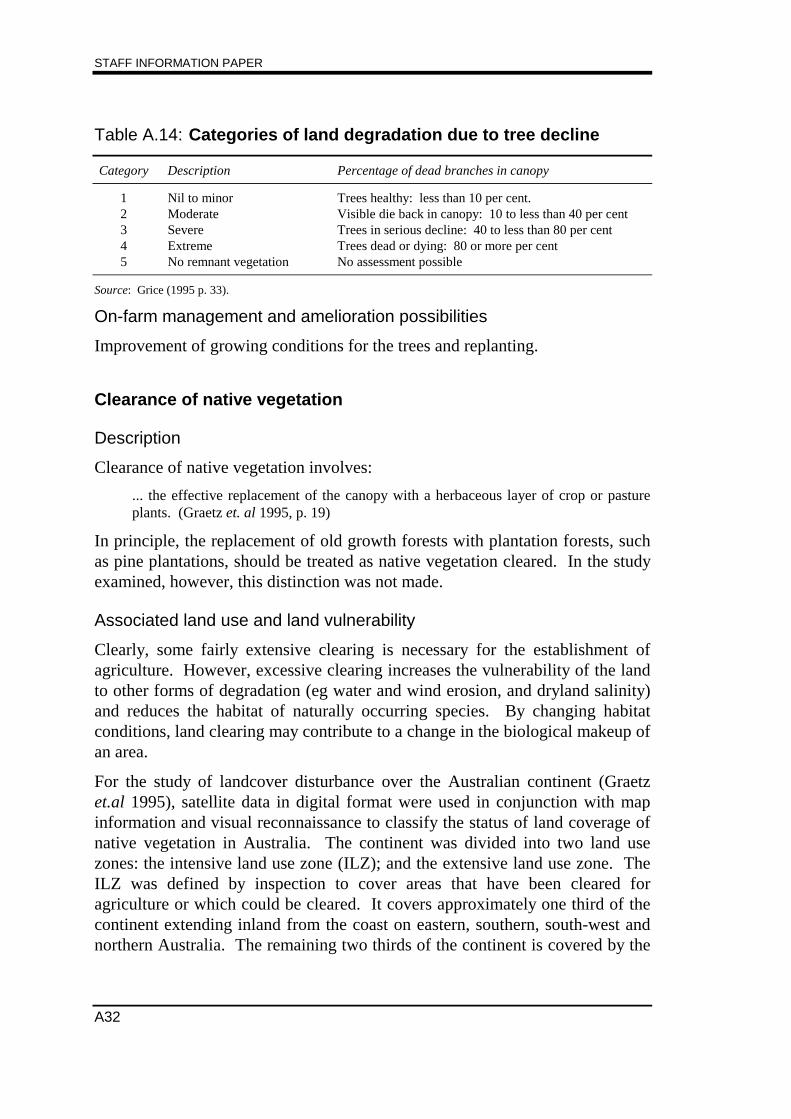
STAFF INFORMATION PAPER
A32
Table A.14: Categories of land degradation due to tree decline
Category Description Percentage of dead branches in canopy
1 Nil to minor Trees healthy: less than 10 per cent.2 Moderate Visible die back in canopy: 10 to less than 40 per cent3 Severe Trees in serious decline: 40 to less than 80 per cent4 Extreme Trees dead or dying: 80 or more per cent5 No remnant vegetation No assessment possible
Source: Grice (1995 p. 33).
On-farm management and amelioration possibilities
Improvement of growing conditions for the trees and replanting.
Clearance of native vegetation
Description
Clearance of native vegetation involves:
... the effective replacement of the canopy with a herbaceous layer of crop or pastureplants. (Graetz et. al 1995, p. 19)
In principle, the replacement of old growth forests with plantation forests, suchas pine plantations, should be treated as native vegetation cleared. In the studyexamined, however, this distinction was not made.
Associated land use and land vulnerability
Clearly, some fairly extensive clearing is necessary for the establishment ofagriculture. However, excessive clearing increases the vulnerability of the landto other forms of degradation (eg water and wind erosion, and dryland salinity)and reduces the habitat of naturally occurring species. By changing habitatconditions, land clearing may contribute to a change in the biological makeup ofan area.
For the study of landcover disturbance over the Australian continent (Graetzet.al 1995), satellite data in digital format were used in conjunction with mapinformation and visual reconnaissance to classify the status of land coverage ofnative vegetation in Australia. The continent was divided into two land usezones: the intensive land use zone (ILZ); and the extensive land use zone. TheILZ was defined by inspection to cover areas that have been cleared foragriculture or which could be cleared. It covers approximately one third of thecontinent extending inland from the coast on eastern, southern, south-west andnorthern Australia. The remaining two thirds of the continent is covered by the
APPENDIX A: CLASSIFICATION OF AGRICULTURAL LAND DEGRADATION IN AUSTRALIA
A33
extensive land use zone (ELZ). The most common form of agriculture in theELZ is extensive pastoral activity that is characterised by the grazing on native(or naturalised3) pasture. The ELZ also covers land made over to communitygroups, unallocated crown land and outback communities. The areas coveredby the ILZ and the ELZ is provided in Table A.15.
Table A.15: Australia-wide coverage of land use zone categories
square kms per cent
Intensive landuse zone 2 983 908 39Extensive landuse zone 4 708 092 61Total 7 692 000 100
Source: Graetz, Wilson and Cambell (1995, p. 20).
Intensity of coverage and base classification
The coverage of native vegetation in the ILZ was divided into one of fourcategories (see Table A.16).
Each category identified in the inventory of native vegetation occurrence in theILZ is determined by an analysis of vegetation coverage as it might occurnaturally. Nevertheless, as mentioned, the methodology adopted does notdistinguish between native and re-afforested areas, with both being classified asuncleared.
The study classified the ELZ into three disturbance classes — slight, substantialand significant. The allocation of the land to one of these three classes wasintended to reflect the contemporary level of disturbance imposed by the twoprincipal agents of land use: grazing of domestic stock; and to a lesser extentrepeated burning (Graetz et. al 1995, p 21).
Off-farm effects
Naturally occurring vegetation is site specific. However, off-site effects thatcan occur from clearing include induced salinity in the forest catchment as watertables rise, reduced biological diversity that may have an anthropocentricrelevance (eg insect eating bats, native flowers for honey bee populations), andpollution arising from soil erosion that follows from land clearing. A property
3 Naturalised pasture refers to introduced pastures that are largely self maintaining under
natural growing conditions.

STAFF INFORMATION PAPER
A34
would have limited scope for containing the effects of clearance within theboundaries of a single land holding and those off-site may also have limitedscope for ameliorating the effects of land clearance elsewhere.
Table A.16: Categories of clearance of native vegetation in theintensive land use zone
Category Description Coverage criteria
1 Uncleared Having an intact canopy relative to all the remnants ofany landcover type. For landcover types with open andsparse canopy types (< 30 per cent of projected foliagecover) it is difficult to separate clearing, the loss ofoverstory, from the effects of overgrazing.
2 Thinned An intermediate class of tree cover between unclearedand cleared.
3 Cleared The effective replacement of the canopy with aherbaceous layer of crop or pasture. The overstory wasassessed to be reduced to < 5 per cent of assessednaturally intact canopy. That is, scattered or no trees.
4 Naturally occurringgrasslands and indeterminate
Assigned to accommodate two cases:(i) where an allocation relating to canopy change wasnot meaningfull eg naturally occurring grassland; and(ii) where technical difficulties prevented fullidentification (the less important of the two cases).
Source: Graetz, Wilson and Cambell (1995, p.19–20).
On-farm management and amelioration possibilities
Vegetation clearance lowers one element of the biological resource available toan individual holding. Where that clearance negatively affects farmproductivity land managers have available the prospect of re-establishing somenative vegetation. However, from the point of view of farm productivity, theappropriate action might be to establish substitute farming systems (egperennials, salt interception and drainage systems). For this reason, theimprovement of productivity would not necessarily involve the re-establish ofnative land cover.
APPENDIX A: CLASSIFICATION OF AGRICULTURAL LAND DEGRADATION IN AUSTRALIA
A35
Feral and other animal invasion4
Description
Feral animals include: the rabbit; fox; cat; and pig which are the most importantin terms of biotic impoverishment on a continental scale (Graetz et al. 1995,p. 22). Other species such as the goat, horse, buffalo and camel are not aswidespread or as influential (although they may cause serious degradationproblems in localities where they do congregate). Graetz et. al have assessedthe relative densities of the main feral species across the continent and were ableto establish a relative coding of none, low, moderate and high densities. Inaddition to feral animal invasion, the populations of native animals (eg the redkangaroo — supposedly the most abundant large mammal in the world) maybecome invasive as habitat changes favour certain species. The invasion ofthose native species could also lead to competition for resources and secondarydegradation, such as wind and water erosion following overgrazing, in acomparable way to feral species.
Each invading species damages the environment in different ways with theseverity of the damage being largely based on the ease with which the specieshave been able to establish themselves, crowd out native species (successfullycompeting for food and space), or prey on native and other species with littlenatural protection.
Off-farm effects
The problem of species invasion is not easily confined by the boundaries ofindividual land holdings. As such, the negative effects to agriculture of feralanimals (eg overgrazing of pastures due to rabbit infestation leading toincreased susceptibility of the land to sheet rill and wind erosion, increasedsusceptibility to gully erosion from rabbit burrows, and loss of young stock andsmall native animals to foxes) cannot be practicably contained or excluded bythe actions of individual land managers. The establishment and infestation ofcertain regions by the feral species provides statistical evidence of this. Theincrease in the kangaroo population supported by permanent watering sources inarid areas and improved pasture has similar effects.
4 In additional to feral animal invasion, feral plant, insect and reptile invasion can also be of
concern as a form of environmental degradation.
STAFF INFORMATION PAPER
A36
Dispersed organic chemical residues and farm waste residues
Description
The residues from farm chemicals such as pesticides and weedicides accumulatein the soil. In addition, farms carry organic matter, such as animal wastes, andnutrients, such as phosphorous, and act as a store of these materials (Cullen andBowmer 1995). It has been suggested (Hamblin and Williams 1995) that therehas been a steady accumulation of organic chemical residues since the 1970swhen pesticides came into general use.
The build up of toxins is a form of land degradation in the sense that theirpresence can lower the marketability of farm produce (eg meat containingchemical residues), and reduce the health of waterways (eg through increasingfrequency of algal blooms, loss of native fish populations and the destruction offloodplain and native vegetation).
Chemical residues can come from broadacre farming (eg cotton growing) andintensive rural industries (eg cattle feedlots, piggeries, dairying and wineries(EPA-New South Wales 1993)). At this stage there does not appear to be anidentifiable classification of degradation severity although readings ofstandardised chemical characteristics are made (eg EPA-New SouthWales 1993).
Off-farm effects — pollution of waterways and other aquifers
An off-farm problem arises more generally when chemicals applied to farmland and animal and plant wastes enter the waterways. The residues change thewater quality potentially reducing its downstream value for use by agriculture,other industries and households. The contamination arises directly as waterbecomes unfit for drinking and indirectly as chemical residues enter the foodchain through animal and plant products. The progressive increase in resistanceof weeds, diseases, and pests that chemicals are intended to control, and theexistence of soil erosion and other land degradation in catchment areascontribute to the severity of the problem.
Individual land managers may have little control over the disbursement ofchemicals and farm residues once they are applied on the holding, althoughfarm or region based interception schemes (as adopted for irrigation salinity)may provide one means of restricting environmental flows. Once farm run-offenters the water ways it mixes with all other water and material entering thesystem and is dispersed widely. Users of the system may not be able to easilyexclude themselves from the effects of the secondary pollution.
B1
APPENDIX BCLASSIFICATION OF AGRICULTURAL REGIONSIN NEW SOUTH WALES
B.1 Introduction
Chapter 3 discusses the need for information about the biogeographiccharacteristics of each region in order to evaluate environmental quality in aneconomic and ecologically meaningful way. In that chapter, reference wasmade to the use of the Interim Biogeographical Regionalisation (IBRA) ofAustralia (Thackway and Cresswell 1995) to combine regional land useinformation from the ABS census of agricultural establishments and the NewSouth Wales survey of land degradation. This appendix provides details of theclassifications adopted and how they are linked as well as information aboutland use drawn from the respective data sources.
Information about agricultural production is available from the ABS agriculturalcensus classified by Statistical Local Areas (SLAs) which are the spatial units inthe Australian Standard Geographical Classification (ABS Cat. No. 1216.0).Land use and land degradation information is available from the New SouthWales 1987–1988 land degradation survey for about 13 000 data points. Toestablish biogeographic regionalisation using these sources, information fromthe New South Wales survey was first aggregated by the National ResourceInformation Centre (NRIC) from survey data to SLA using GeographicInformation System (GIS) techniques. This provided a comprehensiveagricultural data base at the SLA level of aggregation. The SLA spatial unitsthus provided the central building blocks for the analysis. Secondly,information at the SLA level was aggregated to IBRA biogeographic regionsusing a concordance between SLAs and IBRA regions provided by theAustralian Nature Conservation Agency (ANCA).
The land use picture for the SLAs has been drawn from ABS AgriculturalCensus information for 1991–92 and the Soil Conservation Service (SCS)-NewSouth Wales Land Degradation Survey information for 1987–1988. The overallstructure of land use changes sufficiently slowly to enable the information fromboth sources to be combined for analysis. However, the joint use of the twodata sources and the linking of SLA information to biogeographic regions hasnecessitated some classification approximations that are not evident in the broad
STAFF INFORMATION PAPER
B2
regional discussion above but which become more evident once data aredisaggregated to the SLA level.
Section B.2 outlines the IBRA and defines IBRA regions for New South Walesand provides information about land use for these broad regions. Section B.3uses the framework of the SLA classification to discuss the issues relating to thecombination of data sources and land use information. The section alsoprovides a disaggregated analysis of agricultural land coverage of SLAs andland use in New South Wales.
B.2 Interim Biogeographic Regionalisation of Australia
The IBRA was developed for the National Reserve System Conservation Plan(NRSCP) by ANCA in consultation with each state and mainland territory. TheIBRA is based on the biogeographic classifications defined by natureconservation agencies across their respective jurisdictions. The current IBRA(Version 4) contains 80 regions throughout Australia derived on the basis ofexpert knowledge about:
• climate;
• lithology;
• landform;
• vegetation;
• flora and fauna;
• land use; and
• other attributes if needed.
The biogeographic regionalisation of New South Wales is set out in Figure B.1.The name of each region identified in the map is shown in Table B.1 whileAnnex B1 provides standard definitions for each region.
Only three of the 17 regions listed are located entirely in New South Wales (seeTable B.1). This gives a strong indication that regional land management issuesare unlikely to take on an entirely state specific character. With the widespreadoverlapping of regions with state administrative boundaries, the total areacovered by relevant biogeographic regions is about two and a half times the areaof around 801 400 square kilometres falling within New South Wales Stateboundaries. The largest biogeographic regions cover the arid inland areas withthe smaller regions being concentrated around the eastern mountain ranges andcoast.
APPENDIX B: CLASSIFICATION OF AGRICULTURAL REGIONS IN NEW SOUTH WALES
B3
The coverage of regions by agricultural holdings and the average size ofagricultural holding varies substantially (see Table B.2). On the one hand, thebiogeographical regions on the North Coast, and the Central and south coasthave a large number of small agricultural holdings which collectively cover lessthan half of the respective biogeographic regions — well below the averageagricultural holding coverage of 75 per cent for the state as a whole. Thecoastal areas also have a larger than average proportion of area devoted to non-agricultural uses (see Annex B2 for a definition of land uses). For example, inthe South East corner around 79 per cent of the land area is covered by parks,timber and shrub lands which compares to the state average of around22 per cent. The direct influence of farm land management decisions onregional land management is limited in these areas by the low proportion of areacovered by holdings. At the other extreme, regions in the Western areas arecharacterised by a small number of very large holdings covering nearly90 per cent of the land area. Reflecting the arid nature of these regions nearlyall of the land is characterised as native and voluntary pasture (includingnaturalised exotic grasses and legumes used for grazing). Land managementdecisions on agricultural holdings would accordingly be the dominant overallinfluence in regional land management in these areas.
There is substantial variation across the regional groupings between these twoextremes. For example, in the Tablelands group, agricultural holdings in NewEngland and Nandewar occupy over two thirds of the total area whereas in theSouthern highlands around 50 per cent of the area is covered by agriculturalholdings. There are also a larger number of smaller land holdings in theSouthern highlands when compared to the northern tableland regions. Becauseover half of the land in these regions is occupied by agricultural holdings, landmanagement decisions on those holdings would have a major influence onregional land management.
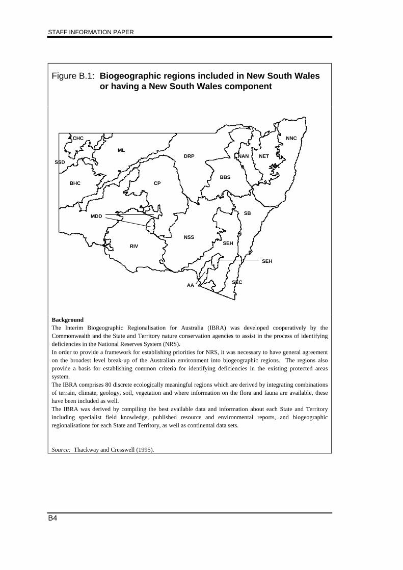
STAFF INFORMATION PAPER
B4
Figure B.1: Biogeographic regions included in New South Walesor having a New South Wales component
BHC
SSD
MLDRP
BBS
NAN NET
NNC
MDD
CP
RIV
NSSSEH
SB
SECAA
SEH
CHC
BackgroundThe Interim Biogeographic Regionalisation for Australia (IBRA) was developed cooperatively by theCommonwealth and the State and Territory nature conservation agencies to assist in the process of identifyingdeficiencies in the National Reserves System (NRS).In order to provide a framework for establishing priorities for NRS, it was necessary to have general agreementon the broadest level break-up of the Australian environment into biogeographic regions. The regions alsoprovide a basis for establishing common criteria for identifying deficiencies in the existing protected areassystem.The IBRA comprises 80 discrete ecologically meaningful regions which are derived by integrating combinationsof terrain, climate, geology, soil, vegetation and where information on the flora and fauna are available, thesehave been included as well.The IBRA was derived by compiling the best available data and information about each State and Territoryincluding specialist field knowledge, published resource and environmental reports, and biogeographicregionalisations for each State and Territory, as well as continental data sets.
Source: Thackway and Cresswell (1995).

APPENDIX B: CLASSIFICATION OF AGRICULTURAL REGIONS IN NEW SOUTH WALES
B5
Table B.1: Biogeographic regions covering New South Walesab
(square kilometres)
Code Region name States covered
Area ofIBRA
region
Coverage ofarea of
Australia
NSWcomponent
of IBRAregion
percent
AA Australian Alps NSW, Vic. 11 718 0.2 4 285BBS Brigalow Belt South Qld, NSW 279 496 3.6 52 458BHC Broken Hill Complex NSW, SA 57 055 0.7 38 222CHC Channel Country Qld, NSW, SA 305 543 4.0 14 289CP Cobar Peneplain NSW 73 501 1.0 73 501DRP Darling Riverine Plain NSW, Qld 105 511 1.4 92 578ML Mulga Lands QLD, NSW 257 850 3.4 65 814MDD Murray-Darling Depression NSW, Vic., SA 197 480 2.6 84 396NAN Nandewar NSW, Qld 27 322 0.4 21 030NET New England Tablelands NSW, Qld 29 347 0.4 27 931NNC NSW North Coast NSW, Qld 60 794 0.8 58 189NSS NSW South West Slopes NSW, Vic. 84 278 1.1 80 874RIV Riverina NSW, Vic. 90 534 1.2 69 068SB Sydney Basin NSW 36 655 0.5 36 655SEC South East Corner Vic., NSW 27 477 0.4 13 459SEH South Eastern Highlands NSW, Vic., ACT 82 576 1.1 48 771SSD Simpson-Strzelecki Dunefields SA, NT, NSW, Qld 277 876 3.6 20 953
Sub total 2 005 013 26.1 802 473
Australia 7 684 968 100.0
a A biogeographic region may cover more than one state. The states covered by a single region are listed indescending order of the area contributed to a biogeographic region.b The total area for Australia and New South Wales shown in the table differ fractionally from the total areas of7 682 300 and 801 600 reported in the Year Book, Australia. The reason for the difference is due to differentprojections used by different spacial data bases.Sources: ABS (1995a), and Thackway and Cresswell (1995).
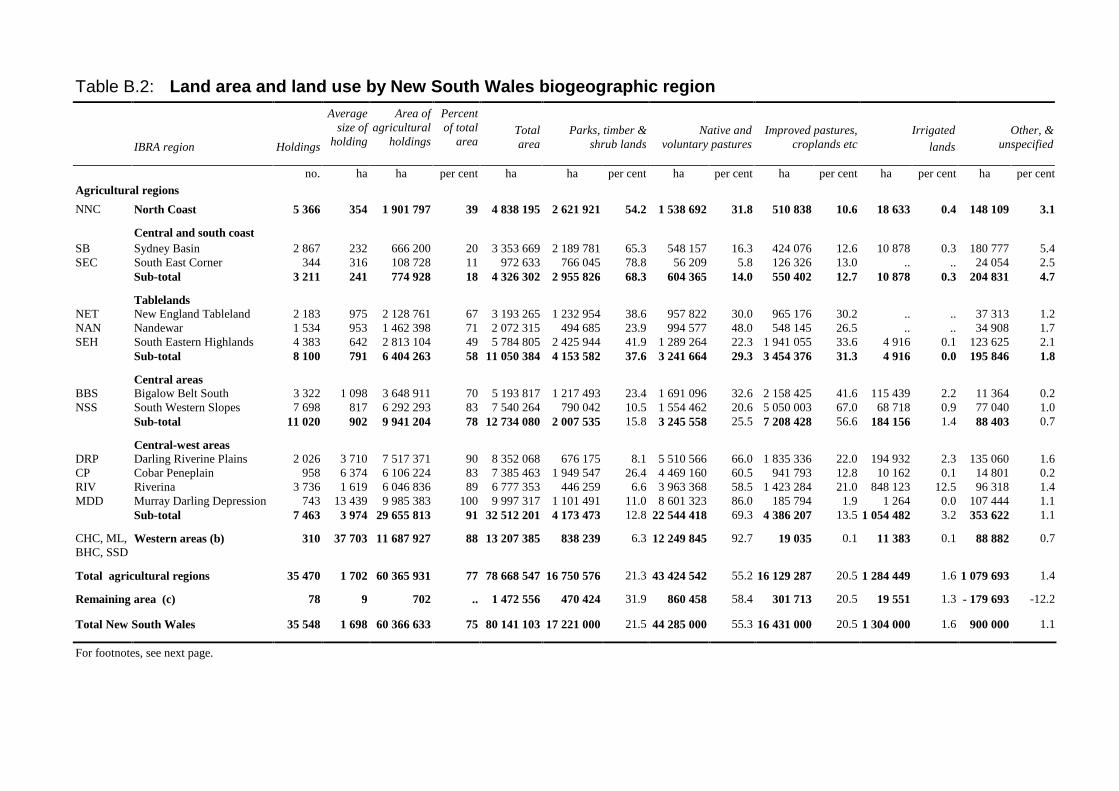
Table B.2: Land area and land use by New South Wales biogeographic region
IBRA region Holdings
Averagesize of
holding
Area ofagricultural
holdings
Percentof total
areaTotalarea
Parks, timber &shrub lands
Native andvoluntary pastures
Improved pastures,croplands etc
Irrigated
lands
Other, &unspecified
no. ha ha per cent ha ha per cent ha per cent ha per cent ha per cent ha per cent
Agricultural regions
NNC North Coast 5 366 354 1 901 797 39 4 838 195 2 621 921 54.2 1 538 692 31.8 510 838 10.6 18 633 0.4 148 109 3.1
Central and south coastSB Sydney Basin 2 867 232 666 200 20 3 353 669 2 189 781 65.3 548 157 16.3 424 076 12.6 10 878 0.3 180 777 5.4SEC South East Corner 344 316 108 728 11 972 633 766 045 78.8 56 209 5.8 126 326 13.0 .. .. 24 054 2.5
Sub-total 3 211 241 774 928 18 4 326 302 2 955 826 68.3 604 365 14.0 550 402 12.7 10 878 0.3 204 831 4.7
TablelandsNET New England Tableland 2 183 975 2 128 761 67 3 193 265 1 232 954 38.6 957 822 30.0 965 176 30.2 .. .. 37 313 1.2NAN Nandewar 1 534 953 1 462 398 71 2 072 315 494 685 23.9 994 577 48.0 548 145 26.5 .. .. 34 908 1.7SEH South Eastern Highlands 4 383 642 2 813 104 49 5 784 805 2 425 944 41.9 1 289 264 22.3 1 941 055 33.6 4 916 0.1 123 625 2.1
Sub-total 8 100 791 6 404 263 58 11 050 384 4 153 582 37.6 3 241 664 29.3 3 454 376 31.3 4 916 0.0 195 846 1.8
Central areasBBS Bigalow Belt South 3 322 1 098 3 648 911 70 5 193 817 1 217 493 23.4 1 691 096 32.6 2 158 425 41.6 115 439 2.2 11 364 0.2NSS South Western Slopes 7 698 817 6 292 293 83 7 540 264 790 042 10.5 1 554 462 20.6 5 050 003 67.0 68 718 0.9 77 040 1.0
Sub-total 11 020 902 9 941 204 78 12 734 080 2 007 535 15.8 3 245 558 25.5 7 208 428 56.6 184 156 1.4 88 403 0.7
Central-west areasDRP Darling Riverine Plains 2 026 3 710 7 517 371 90 8 352 068 676 175 8.1 5 510 566 66.0 1 835 336 22.0 194 932 2.3 135 060 1.6CP Cobar Peneplain 958 6 374 6 106 224 83 7 385 463 1 949 547 26.4 4 469 160 60.5 941 793 12.8 10 162 0.1 14 801 0.2RIV Riverina 3 736 1 619 6 046 836 89 6 777 353 446 259 6.6 3 963 368 58.5 1 423 284 21.0 848 123 12.5 96 318 1.4MDD Murray Darling Depression 743 13 439 9 985 383 100 9 997 317 1 101 491 11.0 8 601 323 86.0 185 794 1.9 1 264 0.0 107 444 1.1
Sub-total 7 463 3 974 29 655 813 91 32 512 201 4 173 473 12.8 22 544 418 69.3 4 386 207 13.5 1 054 482 3.2 353 622 1.1
CHC, ML,BHC, SSD
Western areas (b) 310 37 703 11 687 927 88 13 207 385 838 239 6.3 12 249 845 92.7 19 035 0.1 11 383 0.1 88 882 0.7
Total agricultural regions 35 470 1 702 60 365 931 77 78 668 547 16 750 576 21.3 43 424 542 55.2 16 129 287 20.5 1 284 449 1.6 1 079 693 1.4
Remaining area (c) 78 9 702 .. 1 472 556 470 424 31.9 860 458 58.4 301 713 20.5 19 551 1.3 - 179 693 -12.2
Total New South Wales 35 548 1 698 60 366 633 75 80 141 103 17 221 000 21.5 44 285 000 55.3 16 431 000 20.5 1 304 000 1.6 900 000 1.1
For footnotes, see next page.
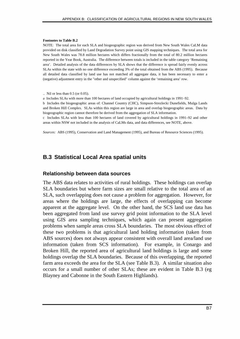
APPENDIX B: CLASSIFICATION OF AGRICULTURAL REGIONS IN NEW SOUTH WALES
B7
Footnotes to Table B.2NOTE: The total area for each SLA and biogeographic region was derived from New South Wales CaLM dataprovided on disk classified by Land Degradation Survey point using GIS mapping techniques. The total area forNew South Wales was 78.8 million hectares which differs fractionally from the total of 80.2 million hectaresreported in the Year Book, Australia. The difference between totals is included in the table category ‘Remainingarea’. Detailed analysis of the data differences by SLA shows that the difference is spread fairly evenly acrossSLAs within the state with no one difference exceeding 3% of the total obtained from the ABS (1995). Becauseall detailed data classified by land use has not matched all aggregate data, it has been necessary to enter a(negative) adjustment entry in the "other and unspecified" column against the ‘remaining area’ row.
.. Nil or less than 0.5 (or 0.05).a Includes SLAs with more than 100 hectares of land occupied by agricultural holdings in 1991–92.b Includes the biogeographic areas of: Channel Country (CHC), Simpson-Strezlecki Dunefields, Mulga Landsand Broken Hill Complex. SLAs within this region are large in area and overlap biogeographic areas. Data bybiogeographic region cannot therefore be derived from the aggregation of SLA information.c Includes SLAs with less than 100 hectares of land covered by agricultural holdings in 1991–92 and otherareas within NSW not included in the analysis of CaLMs data, and data differences, see NOTE, above.
Sources: ABS (1995), Conservation and Land Management (1995), and Bureau of Resource Sciences (1995).
B.3 Statistical Local Area spatial units
Relationship between data sources
The ABS data relates to activities of rural holdings. These holdings can overlapSLA boundaries but where farm sizes are small relative to the total area of anSLA, such overlapping does not cause a problem for aggregation. However, forareas where the holdings are large, the effects of overlapping can becomeapparent at the aggregate level. On the other hand, the SCS land use data hasbeen aggregated from land use survey grid point information to the SLA levelusing GIS area sampling techniques, which again can present aggregationproblems when sample areas cross SLA boundaries. The most obvious effect ofthese two problems is that agricultural land holding information (taken fromABS sources) does not always appear consistent with overall land area/land useinformation (taken from SCS information). For example, in Conargo andBroken Hill, the reported area of agricultural land holdings is large and someholdings overlap the SLA boundaries. Because of this overlapping, the reportedfarm area exceeds the area for the SLA (see Table B.3). A similar situation alsooccurs for a small number of other SLAs; these are evident in Table B.3 (egBlayney and Cabonne in the South Eastern Highlands).
STAFF INFORMATION PAPER
B8
In addition, the boundaries of biogeographic regions do not correspond to SLAboundaries, and not all SLAs fall within a single biogeographic region. Toindicate the biogeographic specialisation of SLAs, the percentage of each SLAfalling within each biogeographic region is reported (see Table B.3). For themajority of SLAs, the specialisation is over 80 per cent, however, for others, thelevel of specialisation is somewhat lower. For example, for Carrathool only halfof the SLA area falls within the Riverina and only 36 per cent of theUnincorporated Far West falls within the Broken Hill Complex. For manybiogeographic regions, gaps and overlaps between region and SLA levelgenerally compensate for one another. Nevertheless, even after taking intoaccount the net effect of all gaps and overlaps, there are still deficiencies. Inparticular agricultural and land use data are not separately available for theAustralian Alps (included in the South east highlands), the Channel Country andthe Simpson-Strzelecki Dunefields (included in the Mulga Lands and theBroken Hill Complex).
Land use
Keeping in mind these methodological issues, the information on land usepresented by biogeographic region in Table B.2 is disaggregated to componentSLAs in this section (see Table B.3). The disparities in farm size, agriculturalholding coverage and land use evident between biogeographic region are alsoevident between SLAs within some biogeographic regions. For example, thereare substantial differences between SLAs within the North Coast biogeographicregion. In this region, while the average coverage of agricultural holdings is39 per cent, agricultural holdings cover less than 20 per cent of areas for SLAssuch as Port Stephens, Coffs Harbour and Nambucca. For this group of SLAs,agricultural land management decisions are likely to have a relatively smallinfluence on overall land management for the area. On the other hand, there isanother group of SLAs in the region in which agricultural holdings cover morethan 50 per cent of area — for Scone the coverage is 80 per cent — andagricultural land management decisions are likely to have a commensuratelylarge effect on regional land management practices.
The major land use in the North Coast biogeographic region is in ‘Parks, timberand shrub lands’, and ‘Native and voluntary pastures’. Together these accountfor around 80 per cent of the region with the relative mix varying betweenSLAs. Some overlap between these areas and farm holdings is likely,particularly as the overall share of farm land rises. However, the extent of thisoverlap is not available.
APPENDIX B: CLASSIFICATION OF AGRICULTURAL REGIONS IN NEW SOUTH WALES
B9
Moving to other regions, the Sydney Basin, South East Corner and SouthEastern Highlands also exhibit substantial variation with respect to the coverageof the area and potential farm influence on overall regional land management.The importance of parks and native pasture in these regions is influenced by theincidence of national parks (eg the Kosciusko National Park would enter intothe South Eastern Highlands which as mentioned above, subsumes theAustralian Alps).
From the tablelands of northern New South Wales, extending inland to thecentral and western areas, the coverage of agricultural land holdings in the totalarea of each SLA is generally high, although some variation between SLAs andbetween regions is evident. For these areas, farm management decisions wouldbe the dominant influence on land management.
Irrigation farming of New South Wales in concentrated in the Riverinabiogeographic region, although there are areas of irrigation farming appearingacross all biogeographic regions (see Table B.3). In the Riverina, farms covernearly 90 per cent of total area with some variation between SLAs. It can beseen that farm size differs substantially between SLAs in this region dependingon the incidence of irrigation farming. For those SLAs in which irrigationfarming is concentrated, the average farm size is well below the regionalaverage, reflecting the intensive nature of irrigation farming as it is currentlypracticed relative to dryland farming.
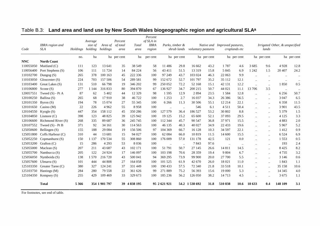
Table B.3: Land area and land use by New South Wales biogeographic region and agricultural SLAa
CodeIBRA region andSLA Holdings
Averagesize of
holdingArea of
holdings
Percentof total
areaTotalarea
Percentof SLA in
IBRAregion
Parks, timber &shrub lands
Native andvoluntary pastures
Improved pastures,croplands etc
Irrigatedlands
Other, & unspecified
no. ha ha per cent ha per cent ha per cent ha per cent ha per cent ha per cent ha per centNNC North Coast110055050 Maitland (C) 111 123 13 641 35 38 549 58 11 486 29.8 16 662 43.2 1 787 4.6 3 685 9.6 4 928 12.8110056400 Port Stephens (S) 106 111 11 724 14 84 224 56 43 411 51.5 13 319 15.8 5 845 6.9 1 242 1.5 20 407 24.2110102700 Dungog (S) 265 378 100 163 45 222 336 100 97 249 43.7 103 024 46.3 22 063 9.9 .. .. .. ..110103050 Gloucester (S) 224 703 157 506 54 289 581 99 152 672 52.7 101 797 35.2 35 112 12.1 .. .. .. ..110103400 Great Lakes (S) 131 510 66 798 19 346 202 99 250 052 72.2 52 168 15.1 42 131 12.2 .. .. 1 850 0.5110106800 Scone (S) 277 1 144 316 833 80 394 870 67 136 927 34.7 200 215 50.7 44 021 11.1 13 706 3.5 .. ..120057551 Tweed (S) - Pt A 87 62 5 402 44 12 329 98 1 595 12.9 2 894 23.5 1 584 12.8 .. .. 6 256 50.7120100250 Ballina (S) 265 68 17 910 38 46 722 100 1 253 2.7 16 037 34.3 26 386 56.5 .. .. 3 047 6.5120101350 Byron (S) 194 78 15 074 27 55 345 100 6 266 11.3 30 506 55.1 12 214 22.1 .. .. 6 358 11.5120101650 Casino (M) 22 226 4 962 55 8 958 100 .. .. 546 6.1 4 511 50.4 .. .. 3 901 43.5120104550 Kyogle (S) 447 354 158 112 45 350 286 100 127 579 36.4 186 527 53.2 30 802 8.8 .. .. 5 379 1.5120104850 Lismore (C) 398 123 48 825 39 125 942 100 19 125 15.2 65 600 52.1 37 093 29.5 .. .. 4 125 3.3120106600 Richmond River (S) 268 335 89 687 36 245 745 100 112 344 45.7 90 547 36.8 37 971 15.5 .. .. 4 883 2.0120107552 Tweed (S) - Pt B 371 92 34 161 30 114 563 100 46 135 40.3 40 027 34.9 22 433 19.6 .. .. 5 967 5.2125050600 Bellingen (S) 155 188 29 084 19 156 506 97 104 369 66.7 16 128 10.3 34 597 22.1 .. .. 1 412 0.9125051800 Coffs Harbour (C) 310 44 13 681 15 94 027 100 62 084 66.0 10 819 11.5 14 600 15.5 .. .. 6 524 6.9125052250 Copmanhurst (S) 150 1 137 170 534 55 308 860 100 176 009 57.0 131 178 42.5 121 0.0 .. .. 1 553 0.5125053200 Grafton (C) 15 286 4 293 53 8 036 100 .. .. 7 843 97.6 .. .. .. .. 193 2.4125055000 Maclean (S) 207 211 43 687 43 102 171 100 51 791 50.7 27 145 26.6 14 811 14.5 .. .. 8 425 8.2125055700 Nambucca (S) 205 122 24 924 17 146 097 100 103 198 70.6 28 359 19.4 9 804 6.7 .. .. 4 735 3.2125056050 Nymboida (S) 138 1 570 216 720 43 500 041 94 369 295 73.9 99 900 20.0 27 700 5.5 .. .. 3 146 0.6125057600 Ulmarra (S) 101 444 44 808 27 164 058 100 101 525 61.9 42 670 26.0 18 021 11.0 .. .. 1 843 1.1125103350 Greater Taree (C) 380 327 124 241 37 331 449 100 190 433 57.5 72 340 21.8 33 518 10.1 .. .. 35 158 10.6125103750 Hastings (M) 284 280 79 558 22 361 626 99 271 889 75.2 56 393 15.6 19 000 5.3 .. .. 14 345 4.0125104350 Kempsey (S) 255 429 109 469 33 329 673 100 185 236 56.2 126 050 38.2 14 713 4.5 .. .. 3 675 1.1
Total 5 366 354 1 901 797 39 4 838 195 95 2 621 921 54.2 1 538 692 31.8 510 838 10.6 18 633 0.4 148 109 3.1
For footnotes, see end of table.
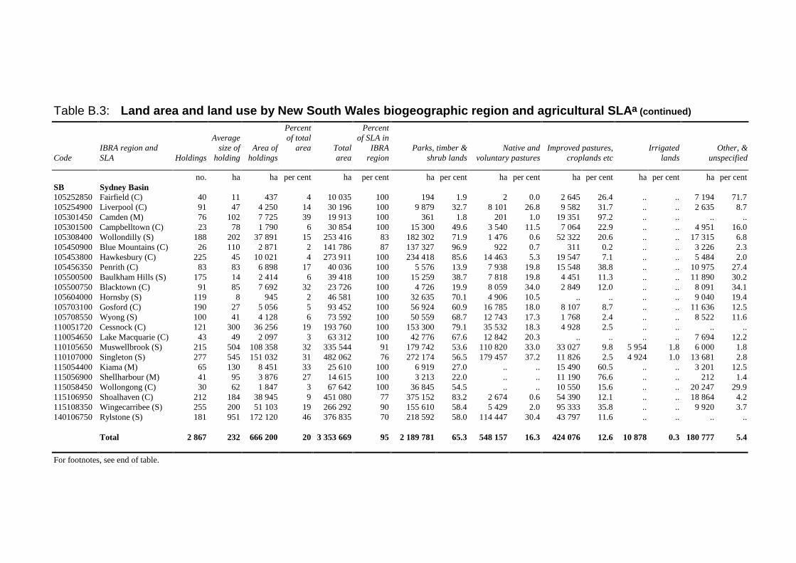
Table B.3: Land area and land use by New South Wales biogeographic region and agricultural SLAa (continued)
CodeIBRA region andSLA Holdings
Averagesize of
holdingArea of
holdings
Percentof total
area Totalarea
Percentof SLA in
IBRAregion
Parks, timber &shrub lands
Native andvoluntary pastures
Improved pastures,croplands etc
Irrigatedlands
Other, &unspecified
no. ha ha per cent ha per cent ha per cent ha per cent ha per cent ha per cent ha per centSB Sydney Basin105252850 Fairfield (C) 40 11 437 4 10 035 100 194 1.9 2 0.0 2 645 26.4 .. .. 7 194 71.7105254900 Liverpool (C) 91 47 4 250 14 30 196 100 9 879 32.7 8 101 26.8 9 582 31.7 .. .. 2 635 8.7105301450 Camden (M) 76 102 7 725 39 19 913 100 361 1.8 201 1.0 19 351 97.2 .. .. .. ..105301500 Campbelltown (C) 23 78 1 790 6 30 854 100 15 300 49.6 3 540 11.5 7 064 22.9 .. .. 4 951 16.0105308400 Wollondilly (S) 188 202 37 891 15 253 416 83 182 302 71.9 1 476 0.6 52 322 20.6 .. .. 17 315 6.8105450900 Blue Mountains (C) 26 110 2 871 2 141 786 87 137 327 96.9 922 0.7 311 0.2 .. .. 3 226 2.3105453800 Hawkesbury (C) 225 45 10 021 4 273 911 100 234 418 85.6 14 463 5.3 19 547 7.1 .. .. 5 484 2.0105456350 Penrith (C) 83 83 6 898 17 40 036 100 5 576 13.9 7 938 19.8 15 548 38.8 .. .. 10 975 27.4105500500 Baulkham Hills (S) 175 14 2 414 6 39 418 100 15 259 38.7 7 818 19.8 4 451 11.3 .. .. 11 890 30.2105500750 Blacktown (C) 91 85 7 692 32 23 726 100 4 726 19.9 8 059 34.0 2 849 12.0 .. .. 8 091 34.1105604000 Hornsby (S) 119 8 945 2 46 581 100 32 635 70.1 4 906 10.5 .. .. .. .. 9 040 19.4105703100 Gosford (C) 190 27 5 056 5 93 452 100 56 924 60.9 16 785 18.0 8 107 8.7 .. .. 11 636 12.5105708550 Wyong (S) 100 41 4 128 6 73 592 100 50 559 68.7 12 743 17.3 1 768 2.4 .. .. 8 522 11.6110051720 Cessnock (C) 121 300 36 256 19 193 760 100 153 300 79.1 35 532 18.3 4 928 2.5 .. .. .. ..110054650 Lake Macquarie (C) 43 49 2 097 3 63 312 100 42 776 67.6 12 842 20.3 .. .. .. .. 7 694 12.2110105650 Muswellbrook (S) 215 504 108 358 32 335 544 91 179 742 53.6 110 820 33.0 33 027 9.8 5 954 1.8 6 000 1.8110107000 Singleton (S) 277 545 151 032 31 482 062 76 272 174 56.5 179 457 37.2 11 826 2.5 4 924 1.0 13 681 2.8115054400 Kiama (M) 65 130 8 451 33 25 610 100 6 919 27.0 .. .. 15 490 60.5 .. .. 3 201 12.5115056900 Shellharbour (M) 41 95 3 876 27 14 615 100 3 213 22.0 .. .. 11 190 76.6 .. .. 212 1.4115058450 Wollongong (C) 30 62 1 847 3 67 642 100 36 845 54.5 .. .. 10 550 15.6 .. .. 20 247 29.9115106950 Shoalhaven (C) 212 184 38 945 9 451 080 77 375 152 83.2 2 674 0.6 54 390 12.1 .. .. 18 864 4.2115108350 Wingecarribee (S) 255 200 51 103 19 266 292 90 155 610 58.4 5 429 2.0 95 333 35.8 .. .. 9 920 3.7140106750 Rylstone (S) 181 951 172 120 46 376 835 70 218 592 58.0 114 447 30.4 43 797 11.6 .. .. .. ..
Total 2 867 232 666 200 20 3 353 669 95 2 189 781 65.3 548 157 16.3 424 076 12.6 10 878 0.3 180 777 5.4
For footnotes, see end of table.
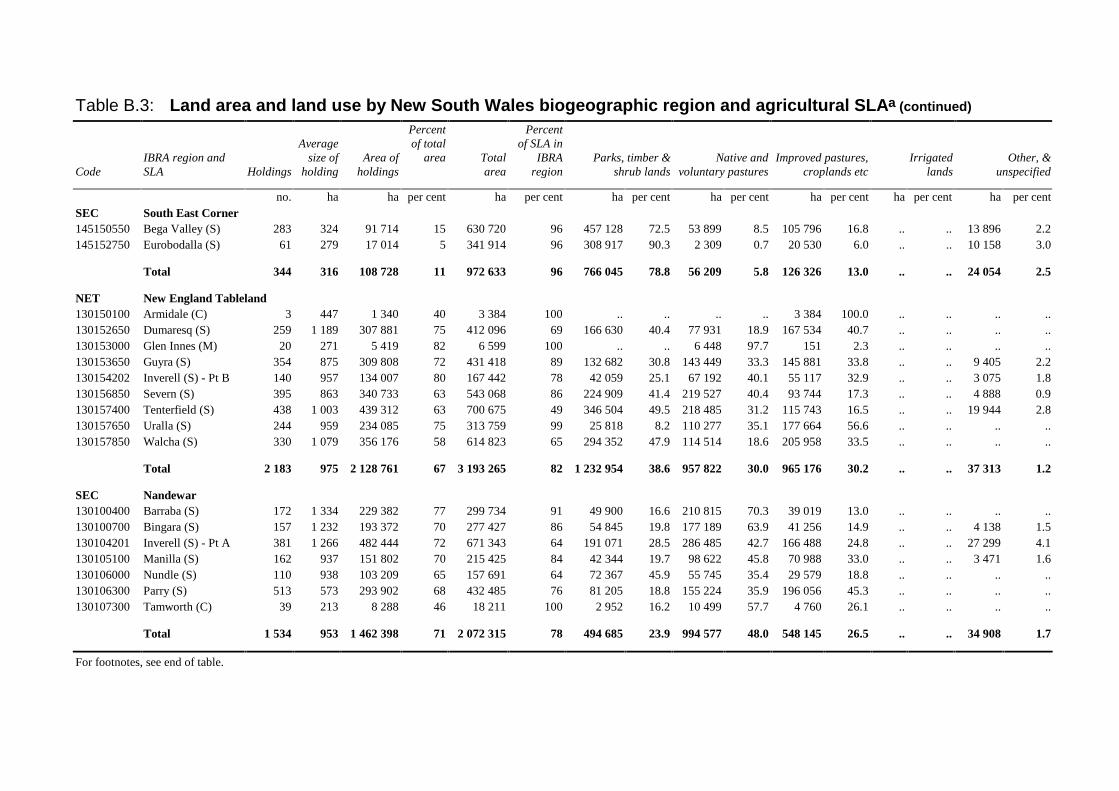
Table B.3: Land area and land use by New South Wales biogeographic region and agricultural SLAa (continued)
CodeIBRA region andSLA Holdings
Averagesize of
holdingArea of
holdings
Percentof total
area Totalarea
Percentof SLA in
IBRAregion
Parks, timber &shrub lands
Native andvoluntary pastures
Improved pastures,croplands etc
Irrigatedlands
Other, &unspecified
no. ha ha per cent ha per cent ha per cent ha per cent ha per cent ha per cent ha per centSEC South East Corner145150550 Bega Valley (S) 283 324 91 714 15 630 720 96 457 128 72.5 53 899 8.5 105 796 16.8 .. .. 13 896 2.2145152750 Eurobodalla (S) 61 279 17 014 5 341 914 96 308 917 90.3 2 309 0.7 20 530 6.0 .. .. 10 158 3.0
Total 344 316 108 728 11 972 633 96 766 045 78.8 56 209 5.8 126 326 13.0 .. .. 24 054 2.5
NET New England Tableland130150100 Armidale (C) 3 447 1 340 40 3 384 100 .. .. .. .. 3 384 100.0 .. .. .. ..130152650 Dumaresq (S) 259 1 189 307 881 75 412 096 69 166 630 40.4 77 931 18.9 167 534 40.7 .. .. .. ..130153000 Glen Innes (M) 20 271 5 419 82 6 599 100 .. .. 6 448 97.7 151 2.3 .. .. .. ..130153650 Guyra (S) 354 875 309 808 72 431 418 89 132 682 30.8 143 449 33.3 145 881 33.8 .. .. 9 405 2.2130154202 Inverell (S) - Pt B 140 957 134 007 80 167 442 78 42 059 25.1 67 192 40.1 55 117 32.9 .. .. 3 075 1.8130156850 Severn (S) 395 863 340 733 63 543 068 86 224 909 41.4 219 527 40.4 93 744 17.3 .. .. 4 888 0.9130157400 Tenterfield (S) 438 1 003 439 312 63 700 675 49 346 504 49.5 218 485 31.2 115 743 16.5 .. .. 19 944 2.8130157650 Uralla (S) 244 959 234 085 75 313 759 99 25 818 8.2 110 277 35.1 177 664 56.6 .. .. .. ..130157850 Walcha (S) 330 1 079 356 176 58 614 823 65 294 352 47.9 114 514 18.6 205 958 33.5 .. .. .. ..
Total 2 183 975 2 128 761 67 3 193 265 82 1 232 954 38.6 957 822 30.0 965 176 30.2 .. .. 37 313 1.2
SEC Nandewar130100400 Barraba (S) 172 1 334 229 382 77 299 734 91 49 900 16.6 210 815 70.3 39 019 13.0 .. .. .. ..130100700 Bingara (S) 157 1 232 193 372 70 277 427 86 54 845 19.8 177 189 63.9 41 256 14.9 .. .. 4 138 1.5130104201 Inverell (S) - Pt A 381 1 266 482 444 72 671 343 64 191 071 28.5 286 485 42.7 166 488 24.8 .. .. 27 299 4.1130105100 Manilla (S) 162 937 151 802 70 215 425 84 42 344 19.7 98 622 45.8 70 988 33.0 .. .. 3 471 1.6130106000 Nundle (S) 110 938 103 209 65 157 691 64 72 367 45.9 55 745 35.4 29 579 18.8 .. .. .. ..130106300 Parry (S) 513 573 293 902 68 432 485 76 81 205 18.8 155 224 35.9 196 056 45.3 .. .. .. ..130107300 Tamworth (C) 39 213 8 288 46 18 211 100 2 952 16.2 10 499 57.7 4 760 26.1 .. .. .. ..
Total 1 534 953 1 462 398 71 2 072 315 78 494 685 23.9 994 577 48.0 548 145 26.5 .. .. 34 908 1.7
For footnotes, see end of table.
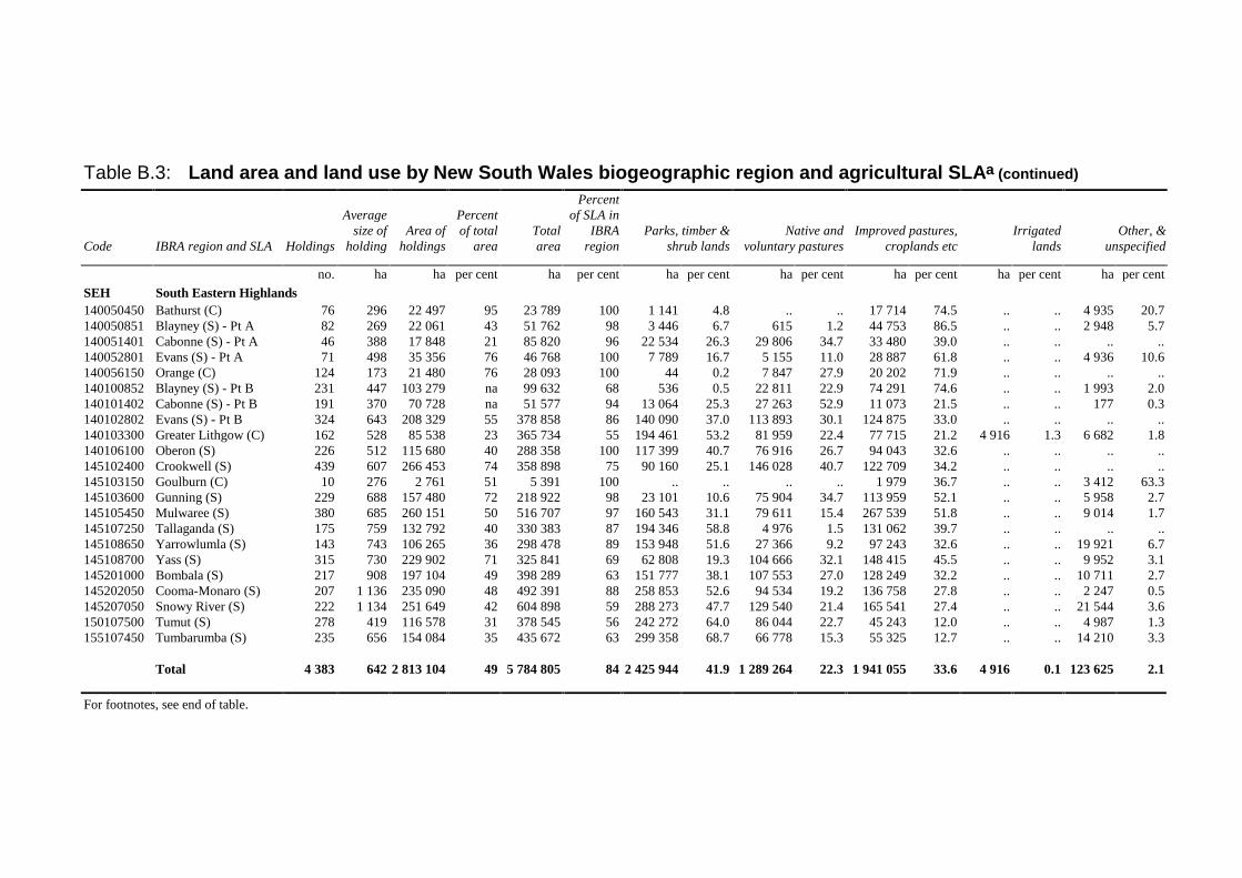
Table B.3: Land area and land use by New South Wales biogeographic region and agricultural SLAa (continued)
Code IBRA region and SLA Holdings
Averagesize of
holdingArea of
holdings
Percentof total
areaTotalarea
Percentof SLA in
IBRAregion
Parks, timber &shrub lands
Native andvoluntary pastures
Improved pastures,croplands etc
Irrigatedlands
Other, &unspecified
no. ha ha per cent ha per cent ha per cent ha per cent ha per cent ha per cent ha per cent
SEH South Eastern Highlands140050450 Bathurst (C) 76 296 22 497 95 23 789 100 1 141 4.8 .. .. 17 714 74.5 .. .. 4 935 20.7140050851 Blayney (S) - Pt A 82 269 22 061 43 51 762 98 3 446 6.7 615 1.2 44 753 86.5 .. .. 2 948 5.7140051401 Cabonne (S) - Pt A 46 388 17 848 21 85 820 96 22 534 26.3 29 806 34.7 33 480 39.0 .. .. .. ..140052801 Evans (S) - Pt A 71 498 35 356 76 46 768 100 7 789 16.7 5 155 11.0 28 887 61.8 .. .. 4 936 10.6140056150 Orange (C) 124 173 21 480 76 28 093 100 44 0.2 7 847 27.9 20 202 71.9 .. .. .. ..140100852 Blayney (S) - Pt B 231 447 103 279 na 99 632 68 536 0.5 22 811 22.9 74 291 74.6 .. .. 1 993 2.0140101402 Cabonne (S) - Pt B 191 370 70 728 na 51 577 94 13 064 25.3 27 263 52.9 11 073 21.5 .. .. 177 0.3140102802 Evans (S) - Pt B 324 643 208 329 55 378 858 86 140 090 37.0 113 893 30.1 124 875 33.0 .. .. .. ..140103300 Greater Lithgow (C) 162 528 85 538 23 365 734 55 194 461 53.2 81 959 22.4 77 715 21.2 4 916 1.3 6 682 1.8140106100 Oberon (S) 226 512 115 680 40 288 358 100 117 399 40.7 76 916 26.7 94 043 32.6 .. .. .. ..145102400 Crookwell (S) 439 607 266 453 74 358 898 75 90 160 25.1 146 028 40.7 122 709 34.2 .. .. .. ..145103150 Goulburn (C) 10 276 2 761 51 5 391 100 .. .. .. .. 1 979 36.7 .. .. 3 412 63.3145103600 Gunning (S) 229 688 157 480 72 218 922 98 23 101 10.6 75 904 34.7 113 959 52.1 .. .. 5 958 2.7145105450 Mulwaree (S) 380 685 260 151 50 516 707 97 160 543 31.1 79 611 15.4 267 539 51.8 .. .. 9 014 1.7145107250 Tallaganda (S) 175 759 132 792 40 330 383 87 194 346 58.8 4 976 1.5 131 062 39.7 .. .. .. ..145108650 Yarrowlumla (S) 143 743 106 265 36 298 478 89 153 948 51.6 27 366 9.2 97 243 32.6 .. .. 19 921 6.7145108700 Yass (S) 315 730 229 902 71 325 841 69 62 808 19.3 104 666 32.1 148 415 45.5 .. .. 9 952 3.1145201000 Bombala (S) 217 908 197 104 49 398 289 63 151 777 38.1 107 553 27.0 128 249 32.2 .. .. 10 711 2.7145202050 Cooma-Monaro (S) 207 1 136 235 090 48 492 391 88 258 853 52.6 94 534 19.2 136 758 27.8 .. .. 2 247 0.5145207050 Snowy River (S) 222 1 134 251 649 42 604 898 59 288 273 47.7 129 540 21.4 165 541 27.4 .. .. 21 544 3.6150107500 Tumut (S) 278 419 116 578 31 378 545 56 242 272 64.0 86 044 22.7 45 243 12.0 .. .. 4 987 1.3155107450 Tumbarumba (S) 235 656 154 084 35 435 672 63 299 358 68.7 66 778 15.3 55 325 12.7 .. .. 14 210 3.3
Total 4 383 642 2 813 104 49 5 784 805 84 2 425 944 41.9 1 289 264 22.3 1 941 055 33.6 4 916 0.1 123 625 2.1
For footnotes, see end of table.
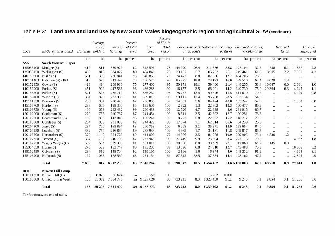
Table B.3: Land area and land use by New South Wales biogeographic region and agricultural SLAa (continued)
Code IBRA region and SLA Holdings
Averagesize of
holdingArea of
holdings
Percentof total
areaTotalarea
Percentof SLA in
IBRAregion
Parks, timber &shrub lands
Native and voluntarypastures
Improved pastures,croplands etc
Irrigatedlands
Other, &unspecified
no. ha ha per cent ha per cent ha per cent ha per cent ha per cent ha per cent ha per centNSS South Western Slopes135055400 Mudgee (S) 419 811 339 979 62 545 596 78 144 020 26.4 211 856 38.8 177 104 32.5 758 0.1 11 857 2.2135058150 Wellington (S) 400 810 324 077 80 404 846 78 23 197 5.7 105 783 26.1 249 461 61.6 8 905 2.2 17 500 4.3140150800 Bland (S) 601 1 309 786 841 93 846 865 72 74 472 8.8 107 686 12.7 664 706 78.5 .. .. .. ..140151403 Cabonne (S) - Pt C 513 670 343 497 75 456 526 96 85 795 18.8 73 193 16.0 289 510 63.4 8 029 1.8 .. ..140152350 Cowra (S) 423 494 208 980 75 277 400 95 50 171 18.1 59 406 21.4 148 255 53.4 16 687 6.0 2 881 1.0140152900 Forbes (S) 451 992 447 566 96 466 288 99 16 157 3.5 66 091 14.2 349 730 75.0 29 364 6.3 4 945 1.1140156200 Parkes (S) 541 898 485 712 83 586 262 96 78 787 13.4 90 876 15.5 411 670 70.2 .. .. 4 929 0.8140158100 Weddin (S) 334 820 273 980 81 339 019 100 59 117 17.4 96 768 28.5 183 134 54.0 .. .. .. ..145101050 Boorowa (S) 238 884 210 478 82 256 095 92 14 361 5.6 104 424 40.8 135 242 52.8 .. .. 2 068 0.8145103700 Harden (S) 238 665 158 300 85 185 601 100 2 322 1.3 22 802 12.3 160 477 86.5 .. .. .. ..145108750 Young (S) 400 659 263 432 99 266 439 100 12 526 4.7 22 898 8.6 231 015 86.7 .. .. .. ..150102000 Coolamon (S) 279 755 210 767 87 241 454 100 8 511 3.5 42 692 17.7 190 251 78.8 .. .. .. ..150102200 Cootamundra (S) 159 893 142 048 95 150 241 100 8 722 5.8 22 802 15.2 118 717 79.0 .. .. .. ..150103500 Gundagai (S) 234 859 201 033 82 244 427 93 17 374 7.1 162 814 66.6 64 239 26.3 .. .. .. ..150104300 Junee (S) 237 700 165 897 83 200 753 100 6 228 3.1 25 871 12.9 168 654 84.0 .. .. .. ..150104950 Lockhart (S) 332 774 256 864 89 288 933 100 4 985 1.7 34 131 11.8 249 817 86.5 .. .. .. ..150105800 Narrandera (S) 320 1 140 364 725 89 411 009 72 14 336 3.5 81 938 19.9 309 905 75.4 4 830 1.2 .. ..150107350 Temora (S) 304 792 240 793 87 277 948 100 27 419 9.9 23 394 8.4 222 173 79.9 .. .. 4 962 1.8150107750 Wagga Wagga (C) 569 684 389 305 81 481 011 100 38 338 8.0 130 469 27.1 312 060 64.9 145 0.0 .. ..155054050 Hume (S) 270 569 153 747 80 193 200 89 13 096 6.8 24 610 12.7 145 488 75.3 .. .. 10 006 5.2155102450 Culcairn (S) 264 552 145 704 92 159 197 100 2 596 1.6 6 374 4.0 145 232 91.2 .. .. 4 995 3.1155103900 Holbrook (S) 172 1 038 178 569 68 261 154 64 87 512 33.5 37 584 14.4 123 162 47.2 .. .. 12 895 4.9
Total 7 698 817 6 292 293 83 7 540 264 90 790 042 10.5 1 554 462 20.6 5 050 003 67.0 68 718 0.9 77 040 1.0
BHC Broken Hill Comp.160101250 Broken Hill (C) 3 8 875 26 624 na 6 752 100 .. .. 6 752 100.0 .. .. .. .. .. ..160108809 Unincorp. Far West 150 51 032 7 654 776 na 9 127 020 36 733 213 8.0 8 323 450 91.2 9 248 0.1 9 854 0.1 51 255 0.6
Total 153 50 205 7 681 400 84 9 133 773 68 733 213 8.0 8 330 202 91.2 9 248 0.1 9 854 0.1 51 255 0.6
For footnotes, see end of table.
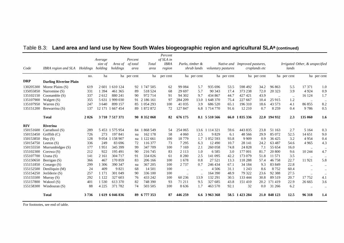
Table B.3: Land area and land use by New South Wales biogeographic region and agricultural SLAa (continued)
Code IBRA region and SLA Holdings
Averagesize of
holdingArea of
holdings
Percentof total
areaTotalarea
Percentof SLA in
IBRAregion
Parks, timber &shrub lands
Native andvoluntary pastures
Improved pastures,croplands etc
Irrigatedlands
Other, & unspecified
no. ha ha per cent ha per cent ha per cent ha per cent ha per cent ha per cent ha per cent
DRP Darling Riverine Plain130205300 Moree Plains (S) 619 2 601 1 610 124 92 1 747 505 62 99 084 5.7 935 696 53.5 598 492 34.2 96 863 5.5 17 371 1.0135055850 Narromine (S) 331 1 394 461 365 89 518 524 68 29 697 5.7 90 343 17.4 373 238 72.0 20 323 3.9 4 924 0.9135102150 Coonamble (S) 337 2 612 880 241 90 972 714 91 94 302 9.7 434 867 44.7 427 421 43.9 .. .. 16 124 1.7135107900 Walgett (S) 355 5 631 1 999 030 91 2 186 161 97 284 209 13.0 1 648 370 75.4 227 667 10.4 25 915 1.2 .. ..135107950 Warren (S) 247 3 640 899 157 85 1 054 293 100 41 035 3.9 686 520 65.1 196 310 18.6 43 573 4.1 86 855 8.2135151200 Brewarrina (S) 137 12 171 1 667 454 89 1 872 872 72 127 847 6.8 1 714 770 91.6 12 210 0.7 8 259 0.4 9 786 0.5
Total 2 026 3 710 7 517 371 90 8 352 068 82 676 175 8.1 5 510 566 66.0 1 835 336 22.0 194 932 2.3 135 060 1.6
RIV Riverina150151600 Carrathool (S) 289 5 453 1 575 954 84 1 868 549 54 254 065 13.6 1 114 321 59.6 443 835 23.8 51 163 2.7 5 164 0.3150153450 Griffith (C) 726 273 197 841 na 162 178 58 4 060 2.5 9 829 6.1 48 566 29.9 85 072 52.5 14 651 9.0150153850 Hay (S) 128 9 054 1 158 907 na 1 122 661 100 18 779 1.7 1 052 593 93.8 9 909 0.9 36 425 3.2 4 954 0.4150154750 Leeton (S) 336 249 83 696 72 116 377 73 7 295 6.3 12 490 10.7 28 141 24.2 63 487 54.6 4 965 4.3150155550 Murrumbidgee (S) 177 1 951 345 399 99 347 709 100 7 169 2.1 260 058 74.8 24 828 7.1 55 654 16.0 .. ..155102300 Corowa (S) 212 922 195 491 90 216 745 83 2 113 1.0 6 585 3.0 177 001 81.7 20 800 9.6 10 244 4.7155107700 Urana (S) 141 2 161 304 717 91 334 026 61 8 280 2.5 141 095 42.2 173 079 51.8 11 571 3.5 .. ..155150650 Berrigan (S) 366 467 170 859 83 206 166 100 1 678 0.8 27 521 13.3 118 288 57.4 46 758 22.7 11 921 5.8155151850 Conargo (S) 299 1 306 390 347 na 367 205 100 2 737 0.7 246 434 67.1 34 184 9.3 83 849 22.8 .. ..155152500 Deniliquin (M) 24 409 9 821 68 14 501 100 .. .. 4 506 31.1 1 243 8.6 8 752 60.4 .. ..155154250 Jerilderie (S) 257 1 171 301 049 90 336 100 100 .. .. 164 390 48.9 79 322 23.6 92 388 27.5 .. ..155155500 Murray (S) 292 1 122 327 603 76 433 242 100 60 236 13.9 132 291 30.5 133 444 30.8 89 519 20.7 17 752 4.1155157800 Wakool (S) 401 1 530 613 370 82 748 390 93 71 211 9.5 327 685 43.8 151 410 20.2 171 419 22.9 26 665 3.6155158300 Windouran (S) 88 4 225 371 782 74 503 505 100 8 636 1.7 463 570 92.1 32 0.0 31 266 6.2 .. ..
Total 3 736 1 619 6 046 836 89 6 777 353 87 446 259 6.6 3 963 368 58.5 1 423 284 21.0 848 123 12.5 96 318 1.4
For footnotes, see end of table.
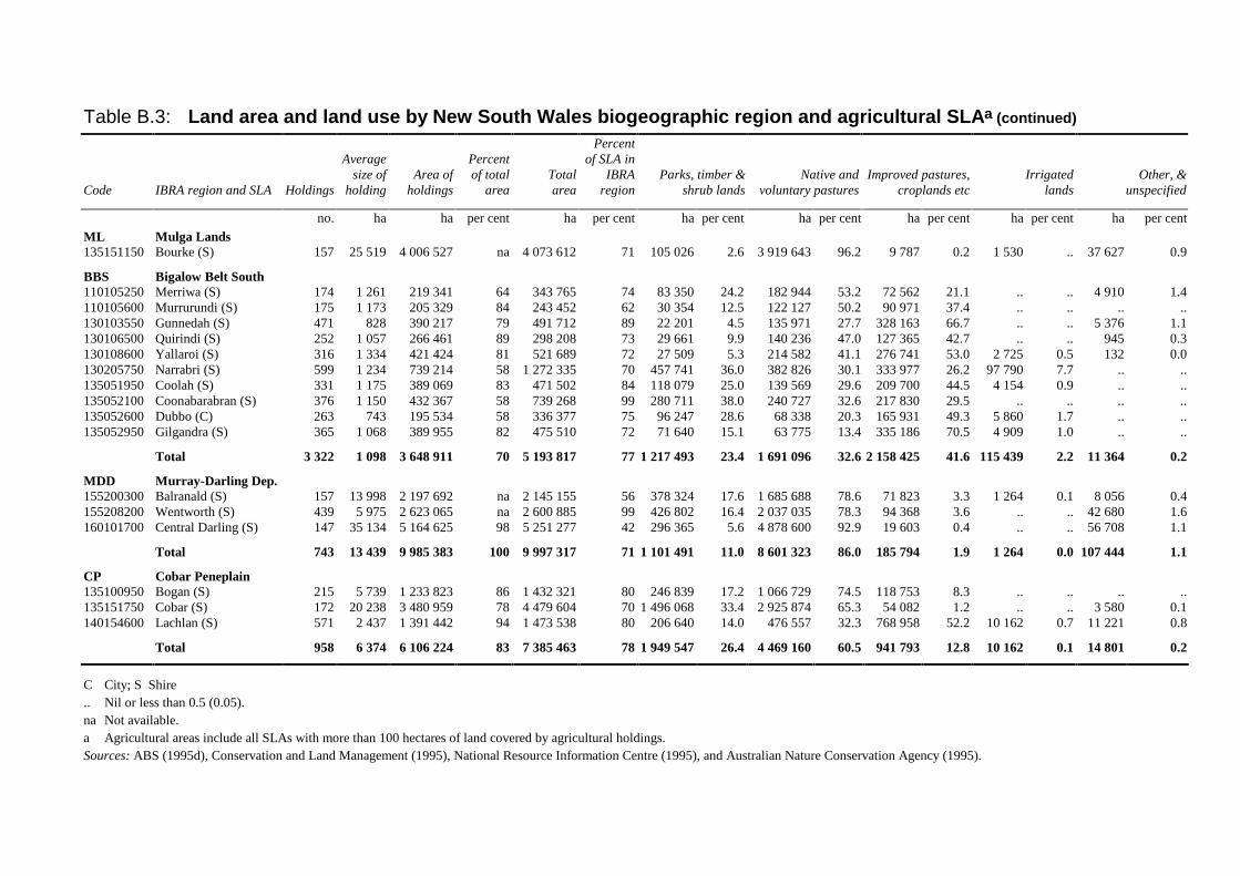
Table B.3: Land area and land use by New South Wales biogeographic region and agricultural SLAa (continued)
Code IBRA region and SLA Holdings
Averagesize of
holdingArea of
holdings
Percentof total
areaTotalarea
Percentof SLA in
IBRAregion
Parks, timber &shrub lands
Native andvoluntary pastures
Improved pastures,croplands etc
Irrigatedlands
Other, &unspecified
no. ha ha per cent ha per cent ha per cent ha per cent ha per cent ha per cent ha per cent
ML Mulga Lands135151150 Bourke (S) 157 25 519 4 006 527 na 4 073 612 71 105 026 2.6 3 919 643 96.2 9 787 0.2 1 530 .. 37 627 0.9
BBS Bigalow Belt South110105250 Merriwa (S) 174 1 261 219 341 64 343 765 74 83 350 24.2 182 944 53.2 72 562 21.1 .. .. 4 910 1.4110105600 Murrurundi (S) 175 1 173 205 329 84 243 452 62 30 354 12.5 122 127 50.2 90 971 37.4 .. .. .. ..130103550 Gunnedah (S) 471 828 390 217 79 491 712 89 22 201 4.5 135 971 27.7 328 163 66.7 .. .. 5 376 1.1130106500 Quirindi (S) 252 1 057 266 461 89 298 208 73 29 661 9.9 140 236 47.0 127 365 42.7 .. .. 945 0.3130108600 Yallaroi (S) 316 1 334 421 424 81 521 689 72 27 509 5.3 214 582 41.1 276 741 53.0 2 725 0.5 132 0.0130205750 Narrabri (S) 599 1 234 739 214 58 1 272 335 70 457 741 36.0 382 826 30.1 333 977 26.2 97 790 7.7 .. ..135051950 Coolah (S) 331 1 175 389 069 83 471 502 84 118 079 25.0 139 569 29.6 209 700 44.5 4 154 0.9 .. ..135052100 Coonabarabran (S) 376 1 150 432 367 58 739 268 99 280 711 38.0 240 727 32.6 217 830 29.5 .. .. .. ..135052600 Dubbo (C) 263 743 195 534 58 336 377 75 96 247 28.6 68 338 20.3 165 931 49.3 5 860 1.7 .. ..135052950 Gilgandra (S) 365 1 068 389 955 82 475 510 72 71 640 15.1 63 775 13.4 335 186 70.5 4 909 1.0 .. ..
Total 3 322 1 098 3 648 911 70 5 193 817 77 1 217 493 23.4 1 691 096 32.6 2 158 425 41.6 115 439 2.2 11 364 0.2
MDD Murray-Darling Dep.155200300 Balranald (S) 157 13 998 2 197 692 na 2 145 155 56 378 324 17.6 1 685 688 78.6 71 823 3.3 1 264 0.1 8 056 0.4155208200 Wentworth (S) 439 5 975 2 623 065 na 2 600 885 99 426 802 16.4 2 037 035 78.3 94 368 3.6 .. .. 42 680 1.6160101700 Central Darling (S) 147 35 134 5 164 625 98 5 251 277 42 296 365 5.6 4 878 600 92.9 19 603 0.4 .. .. 56 708 1.1
Total 743 13 439 9 985 383 100 9 997 317 71 1 101 491 11.0 8 601 323 86.0 185 794 1.9 1 264 0.0 107 444 1.1
CP Cobar Peneplain135100950 Bogan (S) 215 5 739 1 233 823 86 1 432 321 80 246 839 17.2 1 066 729 74.5 118 753 8.3 .. .. .. ..135151750 Cobar (S) 172 20 238 3 480 959 78 4 479 604 70 1 496 068 33.4 2 925 874 65.3 54 082 1.2 .. .. 3 580 0.1140154600 Lachlan (S) 571 2 437 1 391 442 94 1 473 538 80 206 640 14.0 476 557 32.3 768 958 52.2 10 162 0.7 11 221 0.8
Total 958 6 374 6 106 224 83 7 385 463 78 1 949 547 26.4 4 469 160 60.5 941 793 12.8 10 162 0.1 14 801 0.2
C City; S Shire.. Nil or less than 0.5 (0.05).na Not available.a Agricultural areas include all SLAs with more than 100 hectares of land covered by agricultural holdings.Sources: ABS (1995d), Conservation and Land Management (1995), National Resource Information Centre (1995), and Australian Nature Conservation Agency (1995).
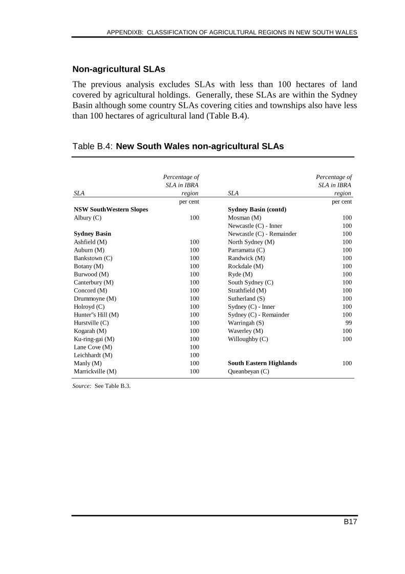
APPENDIXB: CLASSIFICATION OF AGRICULTURAL REGIONS IN NEW SOUTH WALES
B17
Non-agricultural SLAs
The previous analysis excludes SLAs with less than 100 hectares of landcovered by agricultural holdings. Generally, these SLAs are within the SydneyBasin although some country SLAs covering cities and townships also have lessthan 100 hectares of agricultural land (Table B.4).
Table B.4: New South Wales non-agricultural SLAs
SLA
Percentage ofSLA in IBRA
region SLA
Percentage ofSLA in IBRA
regionper cent per cent
NSW SouthWestern Slopes Sydney Basin (contd)Albury (C) 100 Mosman (M) 100
Newcastle (C) - Inner 100Sydney Basin Newcastle (C) - Remainder 100Ashfield (M) 100 North Sydney (M) 100Auburn (M) 100 Parramatta (C) 100Bankstown (C) 100 Randwick (M) 100Botany (M) 100 Rockdale (M) 100Burwood (M) 100 Ryde (M) 100Canterbury (M) 100 South Sydney (C) 100Concord (M) 100 Strathfield (M) 100Drummoyne (M) 100 Sutherland (S) 100Holroyd (C) 100 Sydney (C) - Inner 100Hunter"s Hill (M) 100 Sydney (C) - Remainder 100Hurstville (C) 100 Warringah (S) 99Kogarah (M) 100 Waverley (M) 100Ku-ring-gai (M) 100 Willoughby (C) 100Lane Cove (M) 100Leichhardt (M) 100Manly (M) 100 South Eastern Highlands 100Marrickville (M) 100 Queanbeyan (C)
Source: See Table B.3.
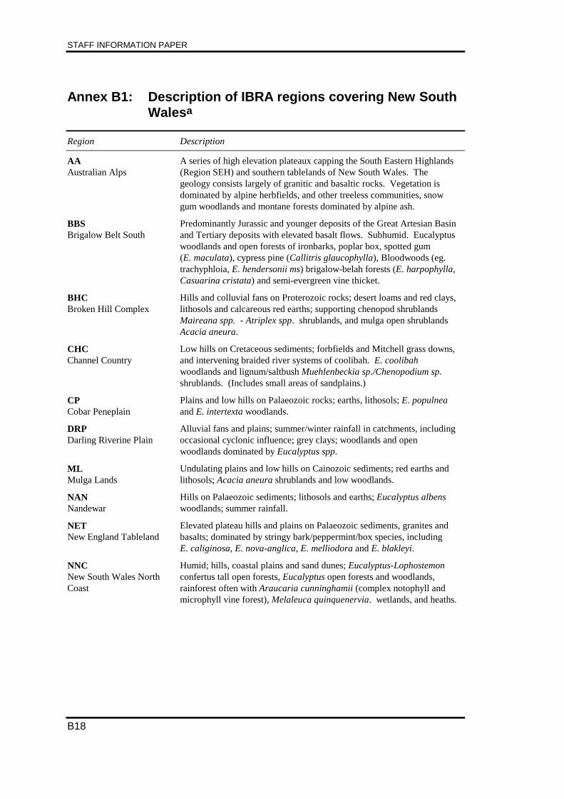
STAFF INFORMATION PAPER
B18
Annex B1: Description of IBRA regions covering New SouthWalesa
Region Description
AAAustralian Alps
A series of high elevation plateaux capping the South Eastern Highlands(Region SEH) and southern tablelands of New South Wales. Thegeology consists largely of granitic and basaltic rocks. Vegetation isdominated by alpine herbfields, and other treeless communities, snowgum woodlands and montane forests dominated by alpine ash.
BBSBrigalow Belt South
Predominantly Jurassic and younger deposits of the Great Artesian Basinand Tertiary deposits with elevated basalt flows. Subhumid. Eucalyptuswoodlands and open forests of ironbarks, poplar box, spotted gum(E. maculata), cypress pine (Callitris glaucophylla), Bloodwoods (eg.trachyphloia, E. hendersonii ms) brigalow-belah forests (E. harpophylla,Casuarina cristata) and semi-evergreen vine thicket.
BHCBroken Hill Complex
Hills and colluvial fans on Proterozoic rocks; desert loams and red clays,lithosols and calcareous red earths; supporting chenopod shrublandsMaireana spp. - Atriplex spp. shrublands, and mulga open shrublandsAcacia aneura.
CHCChannel Country
Low hills on Cretaceous sediments; forbfields and Mitchell grass downs,and intervening braided river systems of coolibah. E. coolibahwoodlands and lignum/saltbush Muehlenbeckia sp./Chenopodium sp.shrublands. (Includes small areas of sandplains.)
CPCobar Peneplain
Plains and low hills on Palaeozoic rocks; earths, lithosols; E. populneaand E. intertexta woodlands.
DRPDarling Riverine Plain
Alluvial fans and plains; summer/winter rainfall in catchments, includingoccasional cyclonic influence; grey clays; woodlands and openwoodlands dominated by Eucalyptus spp.
MLMulga Lands
Undulating plains and low hills on Cainozoic sediments; red earths andlithosols; Acacia aneura shrublands and low woodlands.
NANNandewar
Hills on Palaeozoic sediments; lithosols and earths; Eucalyptus albenswoodlands; summer rainfall.
NETNew England Tableland
Elevated plateau hills and plains on Palaeozoic sediments, granites andbasalts; dominated by stringy bark/peppermint/box species, includingE. caliginosa, E. nova-anglica, E. melliodora and E. blakleyi.
NNCNew South Wales NorthCoast
Humid; hills, coastal plains and sand dunes; Eucalyptus-Lophostemonconfertus tall open forests, Eucalyptus open forests and woodlands,rainforest often with Araucaria cunninghamii (complex notophyll andmicrophyll vine forest), Melaleuca quinquenervia. wetlands, and heaths.

APPENDIXB: CLASSIFICATION OF AGRICULTURAL REGIONS IN NEW SOUTH WALES
B19
Annex B1: Description of IBRA regions covering New SouthWalesa (continued)
Region Description
NSSNew South Wales SouthWest Slopes
An extensive area of foothills and isolated ranges comprising the lowerinland slopes of the Great Dividing Range extending through southernNew South Wales to western Victoria. Vegetation consists of wet/dampsclerophyll forests, peppermint forests and box/ironbark woodlands.
RIVRiverina
An ancient riverine plain and alluvial fans composed of unconsolidatedsediments with evidence of former stream channels. Vegetation consistsof river red gum and black box forests, box woodlands, saltbushshrublands, extensive grasslands and swamp communities.
SBSydney Basin
Mesozoic sandstones and shales; dissected plateaus; forests, woodlandsand heaths; skeletal soils, sands and podzolics.
SECSouth East Corner
A series of deeply dissected near coastal ranges composed of Devoniangranites and Palaeozoic sediments, inland of a series of gently undulatingterraces (piedmont downs) composed of Tertiary sediments and flankedby Quaternary coastal plains, dunefields and inlets. The regional climateis strongly influenced by the Tasman Sea and the close proximity of thecoast to the Great Dividing Range. Vegetation consists of high elevationwoodlands, wet and damp sclerophyll forests interspersed with rain-shadow woodlands in the Snowy River Valley. Lowland and coastalsclerophyll forests, woodlands, warm temperate rainforest and coastalcommunities occur in the lower areas.
SEHSouth Eastern Highlands
Steep dissected and rugged ranges extending across southern and easternVictoria and southern New South Wales. Geology predominantlyPalaeozoic rocks and Mesozoic rocks. Vegetation predominantly wetand dry sclerophyll forests, woodland, minor cool temperate rainforestand minor grassland and herbaceous communities.
SSDSimpson-StrzeleckiDunefields
Arid dunefields and sandplains with sparse shrubland and spinifexhummock grassland, and cane grass on deep sands along dune crests.
a Many of the regions in New South Wales overlap with adjoining states, see Table B.1.Source: Thackway and Cresswell (1995).
STAFF INFORMATION PAPER
B20
Annex B2: Description of land use categories
Parks timber and shrub lands
Nature park and nature reserveLand in public ownership and reserved for the protection of flora and fauna. This land is essentiallyundisturbed.Timber and shrub landsUnlogged forests and previously cleared land which is reverting to native forest. Land used for logging,agricultural and pastoral uses is not included.Logged native forestStands of native forest logged within the last 10 to 20 years.Hardwood plantationLand previously cleared and now covered with a plantation of native hardwood species.Softwood plantationLand previously cleared and now covered with a softwood plantation.
Native and voluntary pastures
Native pastureCleared country or woodland with ground cover of native or naturalised exotic grasses or legumes usedfor grazing.
Improved pasture and croplands etc
Improved pastureCleared or lightly wooded land with a sown ground cover of exotic grasses or legumes and used forgrazing.Cropping - frequentLand regularly cultivated for agricultural production (eg three years of cultivation followed by one yearpasture). Land cultivated for vegetables, flowers or orchards is not included.Cropping infrequentLand used for occasional cultivation (eg one year cultivation followed by three years of pasture).Orchard and vineyardsLand used for the production of fruit and nut trees or vines.Vegetables and flowersLand used for the production of vegetables and flowers.
Irrigated lands
Irrigation - sprayLand irrigated by fixed or travelling spray irrigation systemsIrrigation - floodLand irrigated within bays usually by covering the whole area with a layer of water.
APPENDIXB: CLASSIFICATION OF AGRICULTURAL REGIONS IN NEW SOUTH WALES
B21
Other land uses
UrbanLand within cities or towns including residential and commercial areas.IndustrialLand used for manufacturing or the processing of goods.Quarrying and miningLand used for extractive industries.WaterWater bodies including rivers and lakes but not including offshore or estuarine water bodies.Swamp Swamp land currently under water or with a water table close to the surface; and swampland dryat the time of the survey.
Source: Soil Conservation Service of New South Wales (1989).


C1
APPENDIX CTHE EXTENT OF LAND DEGRADATION INAUSTRALIA
C.1 Introduction
The extent of land degradation in Australia has been of interest over anextended period. This interest has prompted a range of studies. State soilconservation authorities began degradation assessments in the 1930s aimed atpromoting soil conservation measures and establishing soil conservationpriorities (Woods 1983). This appendix reports summary results from publishedstudies of land degradation. Degradation in each state is covered although thepresentation varies with the source of data. The earliest data reported is fromthe erosion survey of New South Wales (Kaleski 1945). There is now quite abody of information about the extent of various types of degradation availablefor periods around the late 1980s and early 1990s. In addition, estimates arebecoming available about the rate of advance of land degradation under currentfarm management practices.
The information presented in this appendix provides an overview of the extentof land degradation in Australia. Section C.2 reports the results of a nationaldegradation study and results of State wide analyses for New South Wales,Victoria, Western Australia and Tasmania. Section C.3 considers the extent ofparticular forms of land degradation, problems encountered in comparingstudies and in the overall measurement of degradation, through review of aselection of special purpose studies. It is in this latter group of studies thatestimates of the advance of degradation are mostly found.
C.2 Estimates of land degradation provided in general studies
Australia-wide degradation study (1975)
Woods (1983) provided information about the incidence of land requiringtreatment or works to ameliorate degradation in respect of the reference year1975. Although now somewhat dated, the study indicates that the concept ofland degradation and its repair was well established and that, with effort,information could be harnessed to provide an economy-wide perspective on

STAFF INFORMATION PAPER
C2
degradation. The published information was drawn from a national degradationassessment carried out by the Commonwealth and States over the period 1975 to1977 in what is known as the Collaborative Soil Conservation Study. To date, afollow up Australia-wide study of degradation using contemporary surveyestimation and measurement techniques has not been made.
The treatment/works approach was adopted for the 1975 survey because it wasassessed at the time that such information would have an immediate applicationin agricultural land management and that information on a degradationinventory basis could not be readily assembled. Although the study providedinformation on areas requiring work, it did not provide judgements concerningthe net benefits of that work, whether the work was likely to be undertaken inthe normal course of land management or whether special policy oradministrative action was required to initiate the work.
The study estimated that a total of 16 per cent (around 80 million hectares) ofagricultural land required amelioration work (see Table C.1). Over two thirdsof this was because of water erosion (including gully, and sheet and rillerosion) with the incidence being concentrated in New South Wales. Otherforms of degradation were also identified in the study. For example, large areasof vegetation decline were apparent in Queensland, New South Wales and theNorthern Territory. In the study, vegetation decline was defined as:
reductions in plant density, plant vigour, the proportion of desirable species and surfacecover which allow soil erosion to accelerate or undesirable species to invade the plantcommunity. (Woods 1983, p. 55)
Vegetation decline occurred in the more arid areas and aspects of it are morepopularly referred to in current studies as ‘woody weed invasion’. Drylandsalinity was also identified as a category of degradation, but the fact that noestimate for this category was reported against New South Wales or Queenslandsuggests that either there was no problem acidity at the time or thatidentification/measurement techniques were not adequate to fully report theincidence of acidity in a national survey. The large ‘other’ category for NewSouth Wales also indicates identification problems. This final catch-allcategory included loss of soil structure, loss of soil fertility and soil pollution.
A substantial amount of information was given about the extent of degradation.However, one of the conclusions of the study was that information on the loss ofproductivity, increased land management cost due to degradation, and the extentand significance of loss of soil structure and fertility was limited.
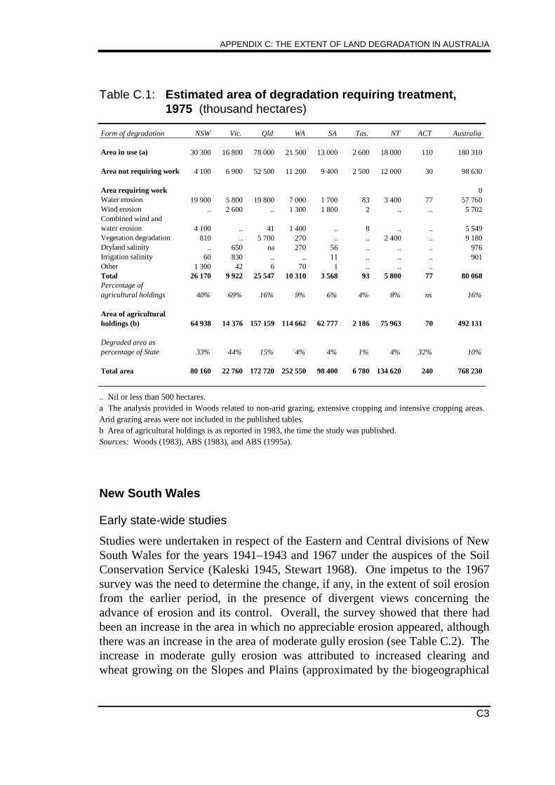
APPENDIX C: THE EXTENT OF LAND DEGRADATION IN AUSTRALIA
C3
Table C.1: Estimated area of degradation requiring treatment,1975 (thousand hectares)
Form of degradation NSW Vic. Qld WA SA Tas. NT ACT Australia
Area in use (a) 30 300 16 800 78 000 21 500 13 000 2 600 18 000 110 180 310
Area not requiring work 4 100 6 900 52 500 11 200 9 400 2 500 12 000 30 98 630
Area requiring work 0Water erosion 19 900 5 800 19 800 7 000 1 700 83 3 400 77 57 760Wind erosion .. 2 600 .. 1 300 1 800 2 .. .. 5 702Combined wind and water erosion 4 100 .. 41 1 400 .. 8 .. .. 5 549Vegetation degradation 810 .. 5 700 270 .. .. 2 400 .. 9 180Dryland salinity .. 650 na 270 56 .. .. .. 976Irrigation salinity 60 830 .. .. 11 .. .. .. 901Other 1 300 42 6 70 1 .. .. ..Total 26 170 9 922 25 547 10 310 3 568 93 5 800 77 80 068Percentage of agricultural holdings 40% 69% 16% 9% 6% 4% 8% ns 16%
Area of agricultural holdings (b) 64 938 14 376 157 159 114 662 62 777 2 186 75 963 70 492 131
Degraded area as percentage of State 33% 44% 15% 4% 4% 1% 4% 32% 10%
Total area 80 160 22 760 172 720 252 550 98 400 6 780 134 620 240 768 230
.. Nil or less than 500 hectares.a The analysis provided in Woods related to non-arid grazing, extensive cropping and intensive cropping areas.Arid grazing areas were not included in the published tables.b Area of agricultural holdings is as reported in 1983, the time the study was published.Sources: Woods (1983), ABS (1983), and ABS (1995a).
New South Wales
Early state-wide studies
Studies were undertaken in respect of the Eastern and Central divisions of NewSouth Wales for the years 1941–1943 and 1967 under the auspices of the SoilConservation Service (Kaleski 1945, Stewart 1968). One impetus to the 1967survey was the need to determine the change, if any, in the extent of soil erosionfrom the earlier period, in the presence of divergent views concerning theadvance of erosion and its control. Overall, the survey showed that there hadbeen an increase in the area in which no appreciable erosion appeared, althoughthere was an increase in the area of moderate gully erosion (see Table C.2). Theincrease in moderate gully erosion was attributed to increased clearing andwheat growing on the Slopes and Plains (approximated by the biogeographical
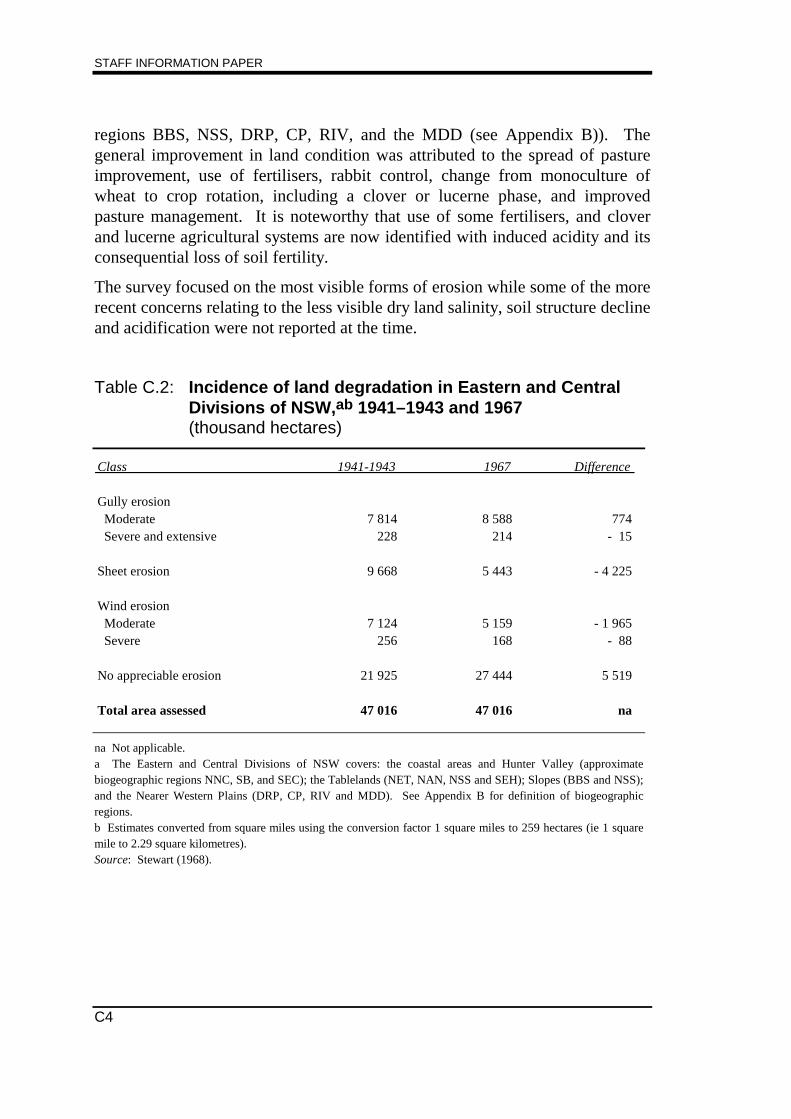
STAFF INFORMATION PAPER
C4
regions BBS, NSS, DRP, CP, RIV, and the MDD (see Appendix B)). Thegeneral improvement in land condition was attributed to the spread of pastureimprovement, use of fertilisers, rabbit control, change from monoculture ofwheat to crop rotation, including a clover or lucerne phase, and improvedpasture management. It is noteworthy that use of some fertilisers, and cloverand lucerne agricultural systems are now identified with induced acidity and itsconsequential loss of soil fertility.
The survey focused on the most visible forms of erosion while some of the morerecent concerns relating to the less visible dry land salinity, soil structure declineand acidification were not reported at the time.
Table C.2: Incidence of land degradation in Eastern and CentralDivisions of NSW,ab 1941–1943 and 1967(thousand hectares)
Class 1941-1943 1967 Difference
Gully erosion Moderate 7 814 8 588 774 Severe and extensive 228 214 - 15
Sheet erosion 9 668 5 443 - 4 225
Wind erosion Moderate 7 124 5 159 - 1 965 Severe 256 168 - 88
No appreciable erosion 21 925 27 444 5 519
Total area assessed 47 016 47 016 na
na Not applicable.a The Eastern and Central Divisions of NSW covers: the coastal areas and Hunter Valley (approximatebiogeographic regions NNC, SB, and SEC); the Tablelands (NET, NAN, NSS and SEH); Slopes (BBS and NSS);and the Nearer Western Plains (DRP, CP, RIV and MDD). See Appendix B for definition of biogeographicregions.b Estimates converted from square miles using the conversion factor 1 square miles to 259 hectares (ie 1 squaremile to 2.29 square kilometres).Source: Stewart (1968).
APPENDIX C: THE EXTENT OF LAND DEGRADATION IN AUSTRALIA
C5
The 1987–1988 Land Degradation Survey
The 1987–1988 Land Degradation Survey was also conducted by the SoilConservation Service of New South Wales (Graham 1989, SCS-New SouthWales 1989). This survey assessed the extent of soil erosion considered in theearlier studies and extended the coverage of land degradation to newdegradation problems such as induced acidity, dryland and irrigation salinityand structural decline. To some extent, these problems arose from efforts toameliorate earlier soil erosion problems and improve farm productivity (egnitrogenous fertilisers and legumes with soil acidification, and heavy farmequipment and cultivation with soil structure decline). The survey differed fromthe Woods study, in that it took an inventory approach to the measurement ofdegradation. The intended uses of the survey results were to provide acomprehensive benchmark for future degradation assessments and the provisionof information for the targeting of programs for the prevention and control ofdegradation.
The survey estimated that over 10 per cent of New South Wales suffers fromsevere soil structure decline or gully erosion and around 4 per cent of the statesuffers from severe induced soil acidity and woody shrub infestation. Althoughthe forgoing surveys are not easily compared at the detailed level, it is evidentthat gully erosion and vegetation degradation have been recognised problemsfor some time.
Four of the most frequently occurring forms of degradation — induced soilacidity, soil structure decline, gully erosion and wind erosion — are locationspecific and therefore largely within the control of individual land holders. Atits initial stages, woody shrub infestation might also be regarded as beingidentified with individual planting or outbreak location(s). However, onceestablished it takes more of a regional dimension, spreading over rivercatchments or whole biogeographic regions. On the other hand, some of thedegradation forms such as dryland and irrigation salinity have a more regionalcharacter and individual farmer decisions will have less influence in reducingdegradation levels. These tend to be among the less frequently recorded formsof degradation and more geographically concentrated. Nevertheless, for eachform of degradation assessed, over three quarters of the state had recorded nil orminor levels.
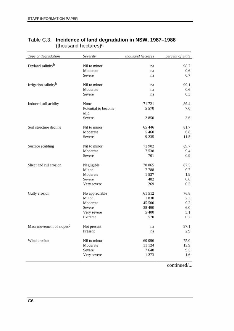
STAFF INFORMATION PAPER
C6
Table C.3: Incidence of land degradation in NSW, 1987–1988(thousand hectares)a
Type of degradation Severity thousand hectares percent of State
Dryland salinityb Nil to minor na 98.7Moderate na 0.6Severe na 0.7
Irrigation salinityb Nil to minor na 99.1Moderate na 0.6Severe na 0.3
Induced soil acidity None 71 721 89.4Potential to becomeacid
5 570 7.0
Severe 2 850 3.6
Soil structure decline Nil to minor 65 446 81.7Moderate 5 460 6.8Severe 9 235 11.5
Surface scalding Nil to minor 71 902 89.7Moderate 7 538 9.4Severe 701 0.9
Sheet and rill erosion Negligible 70 065 87.5Minor 7 788 9.7Moderate 1 537 1.9Severe 482 0.6Very severe 269 0.3
Gully erosion No appreciable 61 512 76.8Minor 1 830 2.3Moderate 45 500 9.2Severe 38 490 6.0Very severe 5 400 5.1Extreme 570 0.7
Mass movement of slopesc Not present na 97.1Present na 2.9
Wind erosion Nil to minor 60 096 75.0Moderate 11 124 13.9Severe 7 648 9.5Very severe 1 273 1.6
continued/...
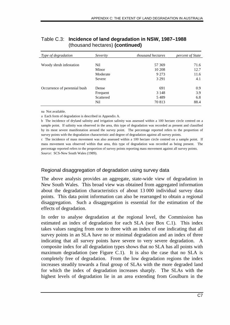
APPENDIX C: THE EXTENT OF LAND DEGRADATION IN AUSTRALIA
C7
Table C.3: Incidence of land degradation in NSW, 1987–1988(thousand hectares) (continued)
Type of degradation Severity thousand hectares percent of State
Woody shrub infestation Nil 57 369 71.6Minor 10 208 12.7Moderate 9 273 11.6Severe 3 291 4.1
Occurrence of perennial bush Dense 691 0.9Frequent 3 148 3.9Scattered 5 489 6.8Nil 70 813 88.4
na Not available.a Each form of degradation is described in Appendix A.b The incidence of dryland salinity and irrigation salinity was assessed within a 100 hectare circle centred on asample point. If salinity was observed in the area, this type of degradation was recorded as present and classifiedby its most severe manifestation around the survey point. The percentage reported refers to the proportion ofsurvey points with the degradation characteristic and degree of degradation against all survey points.c The incidence of mass movement was also assessed within a 100 hectare circle centred on a sample point. Ifmass movement was observed within that area, this type of degradation was recorded as being present. Thepercentage reported refers to the proportion of survey points reporting mass movement against all survey points.Source: SCS-New South Wales (1989).
Regional disaggregation of degradation using survey data
The above analysis provides an aggregate, state-wide view of degradation inNew South Wales. This broad view was obtained from aggregated informationabout the degradation characteristics of about 13 000 individual survey datapoints. This data point information can also be rearranged to obtain a regionaldisaggregation. Such a disaggregation is essential for the estimation of theeffects of degradation.
In order to analyse degradation at the regional level, the Commission hasestimated an index of degradation for each SLA (see Box C.1). This indextakes values ranging from one to three with an index of one indicating that allsurvey points in an SLA have no or minimal degradation and an index of threeindicating that all survey points have severe to very severe degradation. Acomposite index for all degradation types shows that no SLA has all points withmaximum degradation (see Figure C.1). It is also the case that no SLA iscompletely free of degradation. From the low degradation regions the indexincreases steadily towards a final group of SLAs with the more degraded landfor which the index of degradation increases sharply. The SLAs with thehighest levels of degradation lie in an area extending from Goulburn in the
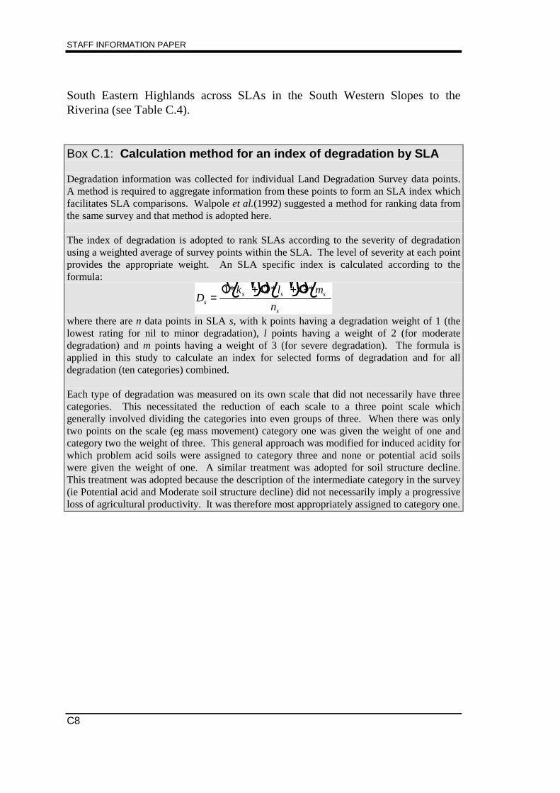
STAFF INFORMATION PAPER
C8
South Eastern Highlands across SLAs in the South Western Slopes to theRiverina (see Table C.4).
Box C.1: Calculation method for an index of degradation by SLA
Degradation information was collected for individual Land Degradation Survey data points.A method is required to aggregate information from these points to form an SLA index whichfacilitates SLA comparisons. Walpole et al.(1992) suggested a method for ranking data fromthe same survey and that method is adopted here.
The index of degradation is adopted to rank SLAs according to the severity of degradationusing a weighted average of survey points within the SLA. The level of severity at each pointprovides the appropriate weight. An SLA specific index is calculated according to theformula:
Dk l m
nss s s
s
=+ +1 2 3* * *����� �
where there are n data points in SLA s, with k points having a degradation weight of 1 (thelowest rating for nil to minor degradation), l points having a weight of 2 (for moderatedegradation) and m points having a weight of 3 (for severe degradation). The formula isapplied in this study to calculate an index for selected forms of degradation and for alldegradation (ten categories) combined.
Each type of degradation was measured on its own scale that did not necessarily have threecategories. This necessitated the reduction of each scale to a three point scale whichgenerally involved dividing the categories into even groups of three. When there was onlytwo points on the scale (eg mass movement) category one was given the weight of one andcategory two the weight of three. This general approach was modified for induced acidity forwhich problem acid soils were assigned to category three and none or potential acid soilswere given the weight of one. A similar treatment was adopted for soil structure decline.This treatment was adopted because the description of the intermediate category in the survey(ie Potential acid and Moderate soil structure decline) did not necessarily imply a progressiveloss of agricultural productivity. It was therefore most appropriately assigned to category one.
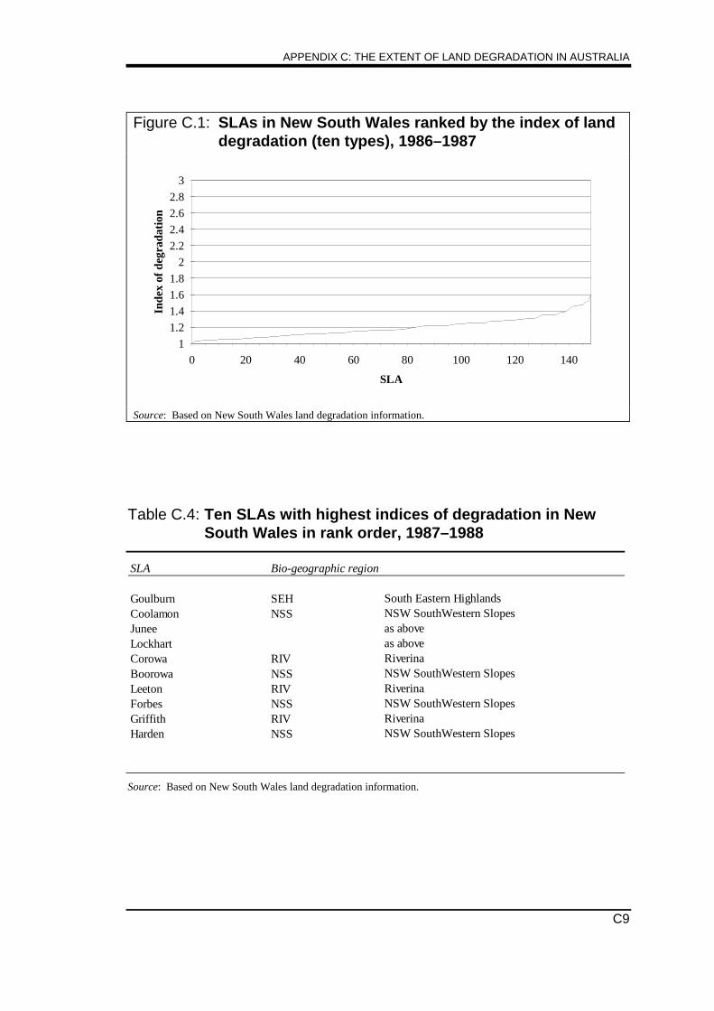
APPENDIX C: THE EXTENT OF LAND DEGRADATION IN AUSTRALIA
C9
Figure C.1: SLAs in New South Wales ranked by the index of landdegradation (ten types), 1986–1987
SLA
Inde
x of
deg
rada
tion
1
1.2
1.4
1.6
1.8
2
2.2
2.4
2.6
2.8
3
0 20 40 60 80 100 120 140
Source: Based on New South Wales land degradation information.
Table C.4: Ten SLAs with highest indices of degradation in NewSouth Wales in rank order, 1987–1988
SLA Bio-geographic region
Goulburn SEH South Eastern HighlandsCoolamon NSS NSW SouthWestern Slopes Junee as aboveLockhart as aboveCorowa RIV RiverinaBoorowa NSS NSW SouthWestern SlopesLeeton RIV RiverinaForbes NSS NSW SouthWestern Slopes Griffith RIV RiverinaHarden NSS NSW SouthWestern Slopes
Source: Based on New South Wales land degradation information.
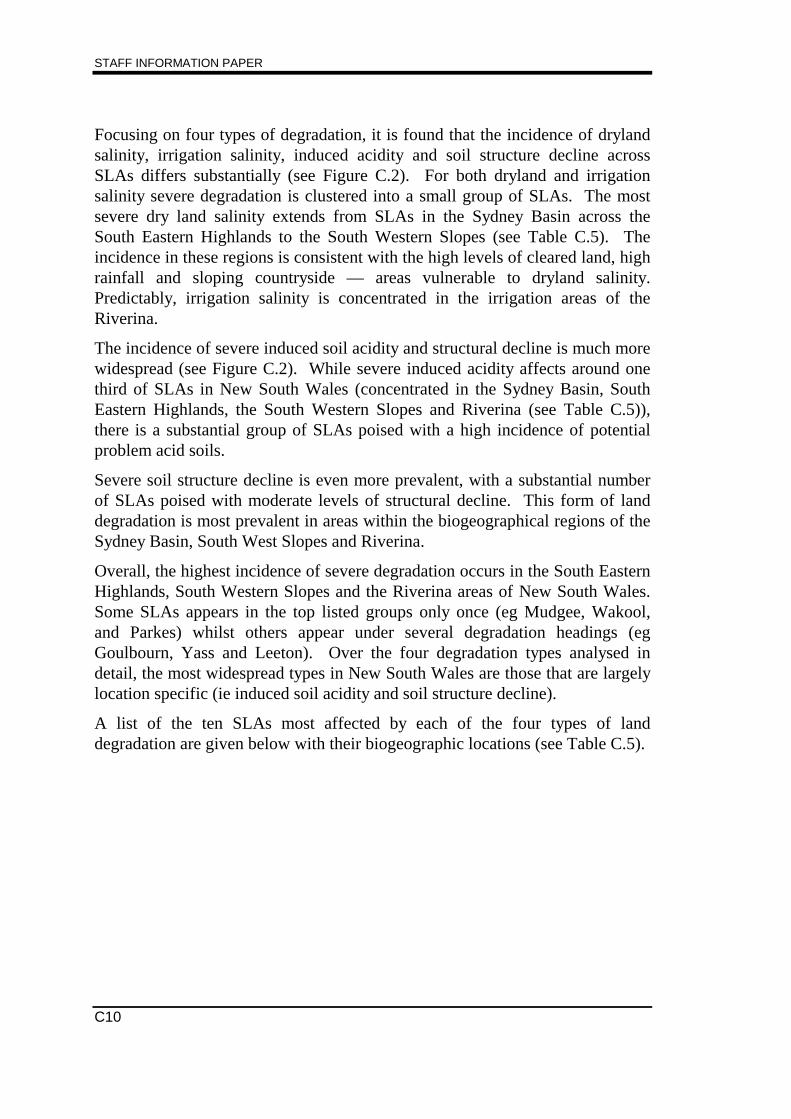
STAFF INFORMATION PAPER
C10
Focusing on four types of degradation, it is found that the incidence of drylandsalinity, irrigation salinity, induced acidity and soil structure decline acrossSLAs differs substantially (see Figure C.2). For both dryland and irrigationsalinity severe degradation is clustered into a small group of SLAs. The mostsevere dry land salinity extends from SLAs in the Sydney Basin across theSouth Eastern Highlands to the South Western Slopes (see Table C.5). Theincidence in these regions is consistent with the high levels of cleared land, highrainfall and sloping countryside — areas vulnerable to dryland salinity.Predictably, irrigation salinity is concentrated in the irrigation areas of theRiverina.
The incidence of severe induced soil acidity and structural decline is much morewidespread (see Figure C.2). While severe induced acidity affects around onethird of SLAs in New South Wales (concentrated in the Sydney Basin, SouthEastern Highlands, the South Western Slopes and Riverina (see Table C.5)),there is a substantial group of SLAs poised with a high incidence of potentialproblem acid soils.
Severe soil structure decline is even more prevalent, with a substantial numberof SLAs poised with moderate levels of structural decline. This form of landdegradation is most prevalent in areas within the biogeographical regions of theSydney Basin, South West Slopes and Riverina.
Overall, the highest incidence of severe degradation occurs in the South EasternHighlands, South Western Slopes and the Riverina areas of New South Wales.Some SLAs appears in the top listed groups only once (eg Mudgee, Wakool,and Parkes) whilst others appear under several degradation headings (egGoulbourn, Yass and Leeton). Over the four degradation types analysed indetail, the most widespread types in New South Wales are those that are largelylocation specific (ie induced soil acidity and soil structure decline).
A list of the ten SLAs most affected by each of the four types of landdegradation are given below with their biogeographic locations (see Table C.5).
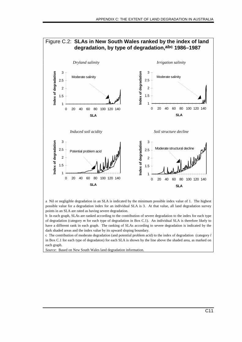
APPENDIX C: THE EXTENT OF LAND DEGRADATION IN AUSTRALIA
C11
Figure C.2: SLAs in New South Wales ranked by the index of landdegradation, by type of degradation,abc 1986–1987
Dryland salinity Irrigation salinity
1
1.5
2
2.5
3
0 20 40 60 80 100 120 140
SLA
Ind
ex o
f d
egra
dat
ion
Moderate salinity
1
1.5
2
2.5
3
0 20 40 60 80 100 120 140
SLA
Ind
ex o
f d
egra
dat
ion
Moderate salinity
Induced soil acidity Soil structure decline
1
1.5
2
2.5
3
0 20 40 60 80 100 120 140
SLA
Ind
ex o
f d
egra
dat
ion
Potential problem acid
1
1.5
2
2.5
3
0 20 40 60 80 100 120 140
SLA
Ind
ex o
f d
egra
dat
ion
Moderate structural decline
a Nil or negligible degradation in an SLA is indicated by the minimum possible index value of 1. The highestpossible value for a degradation index for an individual SLA is 3. At that value, all land degradation surveypoints in an SLA are rated as having severe degradation.b In each graph, SLAs are ranked according to the contribution of severe degradation to the index for each typeof degradation (category m for each type of degradation in Box C.1). An individual SLA is therefore likely tohave a different rank in each graph. The ranking of SLAs according to severe degradation is indicated by thedark shaded areas and the index value by its upward sloping boundary.c The contribution of moderate degradation (and potential problem acid) to the index of degradation (category lin Box C.1 for each type of degradaton) for each SLA is shown by the line above the shaded area, as marked oneach graph.Source: Based on New South Wales land degradation information.
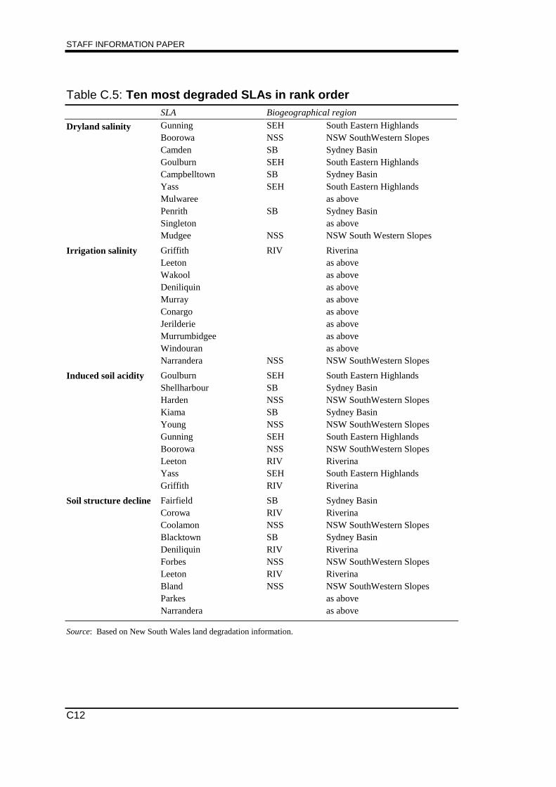
STAFF INFORMATION PAPER
C12
Table C.5: Ten most degraded SLAs in rank orderSLA Biogeographical region
Dryland salinity Gunning SEH South Eastern HighlandsBoorowa NSS NSW SouthWestern SlopesCamden SB Sydney BasinGoulburn SEH South Eastern HighlandsCampbelltown SB Sydney BasinYass SEH South Eastern HighlandsMulwaree as abovePenrith SB Sydney BasinSingleton as aboveMudgee NSS NSW South Western Slopes
Irrigation salinity Griffith RIV RiverinaLeeton as aboveWakool as aboveDeniliquin as aboveMurray as aboveConargo as aboveJerilderie as aboveMurrumbidgee as aboveWindouran as aboveNarrandera NSS NSW SouthWestern Slopes
Induced soil acidity Goulburn SEH South Eastern HighlandsShellharbour SB Sydney BasinHarden NSS NSW SouthWestern SlopesKiama SB Sydney BasinYoung NSS NSW SouthWestern SlopesGunning SEH South Eastern HighlandsBoorowa NSS NSW SouthWestern SlopesLeeton RIV RiverinaYass SEH South Eastern HighlandsGriffith RIV Riverina
Soil structure decline Fairfield SB Sydney BasinCorowa RIV RiverinaCoolamon NSS NSW SouthWestern SlopesBlacktown SB Sydney BasinDeniliquin RIV RiverinaForbes NSS NSW SouthWestern SlopesLeeton RIV RiverinaBland NSS NSW SouthWestern SlopesParkes as aboveNarrandera as above
Source: Based on New South Wales land degradation information.
APPENDIX C: THE EXTENT OF LAND DEGRADATION IN AUSTRALIA
C13
Victoria
Historical accounts of degradation in Victoria extend back to the earliest days ofsettlement (Office of the Commissioner for the Environment — Victoria 1991).According to contemporary assessments, the most visible forms of erosion havebeen substantially reduced and controlled through better land management, asindicated by:
Much of the area used for broadacre cropping is of insignificant or low or inherentsusceptibility to all forms of water erosion, but of low, medium or high susceptibility towind erosion. While clearing, cultivation and fallowing of croplands have promotedwind and water erosion, land management is continually evolving to minimise theseimpacts. (Office of the Commissioner for the Environment — Victoria 1991, p. 146)
and
The establishment of introduced pasture species to replace native grasses adverselyaffected by grazing, and erosion works to counter land degradation initiated during the19th Century has meant that water erosion has diminished as a problem for most landunder permanent pasture. (Office of the Commissioner for the Environment — Victoria1991, p. 164)
Available estimates of the extent of agricultural land degradation in Victoriaindicate that induced acidity and soil structure decline are widespread (see TableC.6). For example, 58 per cent of dry land pasture is assessed as strongly orextremely acid, while around 40 per cent of broadacre cropland and 90 per centof irrigated pasture is assessed as subject to severe soil structure decline. Boththese forms of degradation are farm specific and their extent, in effect, reflectsthe outcome of land management systems adopted with respect to the operationof individual farms.
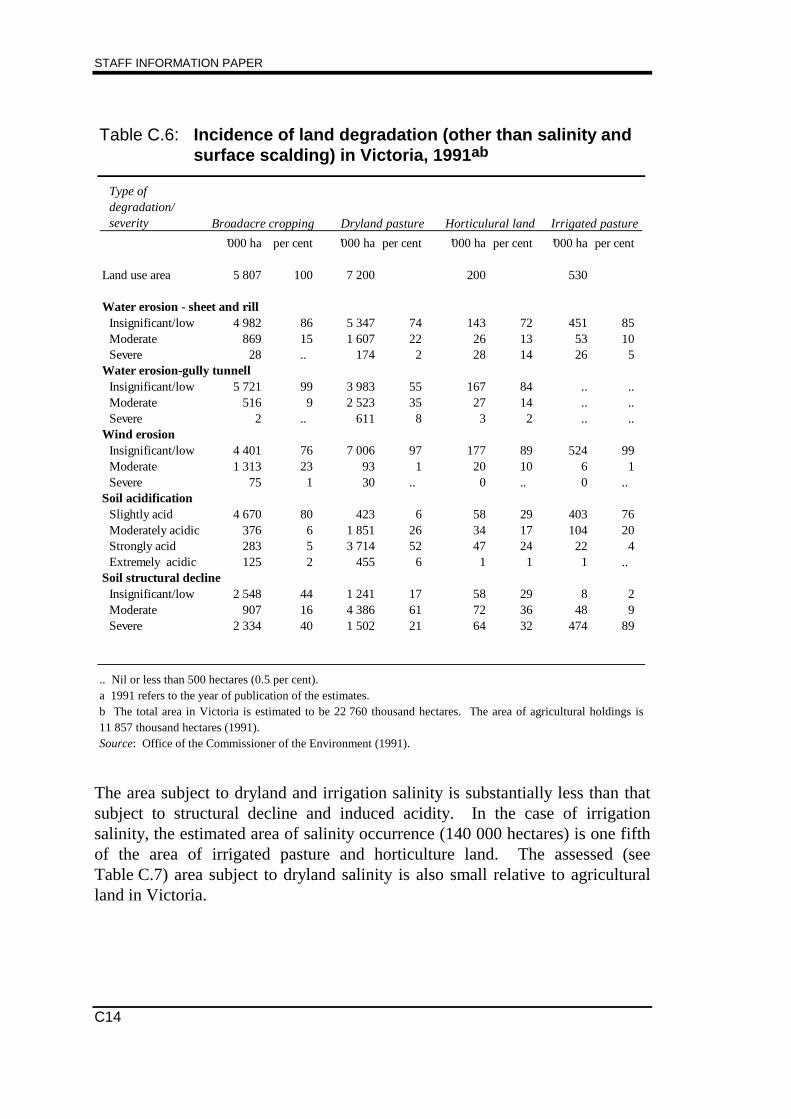
STAFF INFORMATION PAPER
C14
Table C.6: Incidence of land degradation (other than salinity andsurface scalding) in Victoria, 1991ab
Type of degradation/ severity Broadacre cropping Dryland pasture Horticulural land Irrigated pasture
’000 ha per cent ’000 ha per cent ’000 ha per cent ’000 ha per cent
Land use area 5 807 100 7 200 200 530
Water erosion - sheet and rillInsignificant/low 4 982 86 5 347 74 143 72 451 85Moderate 869 15 1 607 22 26 13 53 10Severe 28 .. 174 2 28 14 26 5
Water erosion-gully tunnellInsignificant/low 5 721 99 3 983 55 167 84 .. ..Moderate 516 9 2 523 35 27 14 .. ..Severe 2 .. 611 8 3 2 .. ..
Wind erosionInsignificant/low 4 401 76 7 006 97 177 89 524 99Moderate 1 313 23 93 1 20 10 6 1Severe 75 1 30 .. 0 .. 0 ..
Soil acidificationSlightly acid 4 670 80 423 6 58 29 403 76Moderately acidic 376 6 1 851 26 34 17 104 20Strongly acid 283 5 3 714 52 47 24 22 4Extremely acidic 125 2 455 6 1 1 1 ..
Soil structural declineInsignificant/low 2 548 44 1 241 17 58 29 8 2Moderate 907 16 4 386 61 72 36 48 9Severe 2 334 40 1 502 21 64 32 474 89
.. Nil or less than 500 hectares (0.5 per cent).a 1991 refers to the year of publication of the estimates.b The total area in Victoria is estimated to be 22 760 thousand hectares. The area of agricultural holdings is11 857 thousand hectares (1991).Source: Office of the Commissioner of the Environment (1991).
The area subject to dryland and irrigation salinity is substantially less than thatsubject to structural decline and induced acidity. In the case of irrigationsalinity, the estimated area of salinity occurrence (140 000 hectares) is one fifthof the area of irrigated pasture and horticulture land. The assessed (seeTable C.7) area subject to dryland salinity is also small relative to agriculturalland in Victoria.
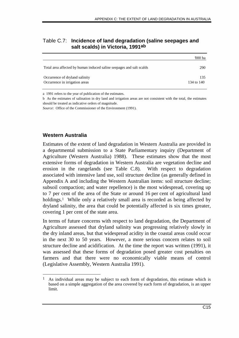
APPENDIX C: THE EXTENT OF LAND DEGRADATION IN AUSTRALIA
C15
Table C.7: Incidence of land degradation (saline seepages andsalt scalds) in Victoria, 1991ab
’000 ha
Total area affected by human induced saline seepages and salt scalds 290
Occurrence of dryland salinity 135Occurrence in irrigation areas 134 to 140
a 1991 refers to the year of publication of the estimates.b As the estimates of salination in dry land and irrigation areas are not consistent with the total, the estimatesshould be treated as indicative orders of magnitude.Source: Office of the Commissioner of the Environment (1991).
Western Australia
Estimates of the extent of land degradation in Western Australia are provided ina departmental submission to a State Parliamentary inquiry (Department ofAgriculture (Western Australia) 1988). These estimates show that the mostextensive forms of degradation in Western Australia are vegetation decline anderosion in the rangelands (see Table C.8). With respect to degradationassociated with intensive land use, soil structure decline (as generally defined inAppendix A and including the Western Australian items: soil structure decline;subsoil compaction; and water repellence) is the most widespread, covering upto 7 per cent of the area of the State or around 16 per cent of agricultural landholdings.1 While only a relatively small area is recorded as being affected bydryland salinity, the area that could be potentially affected is six times greater,covering 1 per cent of the state area.
In terms of future concerns with respect to land degradation, the Department ofAgriculture assessed that dryland salinity was progressing relatively slowly inthe dry inland areas, but that widespread acidity in the coastal areas could occurin the next 30 to 50 years. However, a more serious concern relates to soilstructure decline and acidification. At the time the report was written (1991), itwas assessed that these forms of degradation posed greater cost penalties onfarmers and that there were no economically viable means of control(Legislative Assembly, Western Australia 1991).
1 As individual areas may be subject to each form of degradation, this estimate which is
based on a simple aggregation of the area covered by each form of degradation, is an upperlimit.
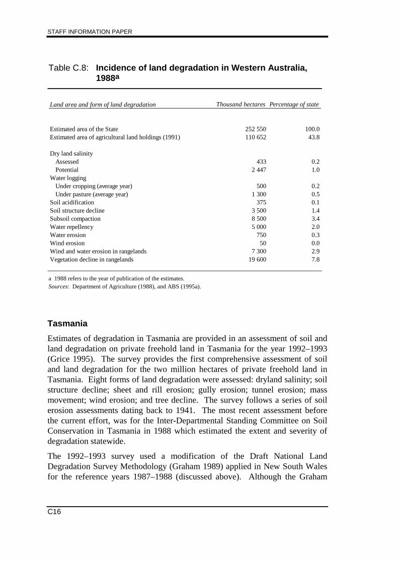
STAFF INFORMATION PAPER
C16
Table C.8: Incidence of land degradation in Western Australia,1988a
Land area and form of land degradation Thousand hectares Percentage of state
Estimated area of the State 252 550 100.0Estimated area of agricultural land holdings (1991) 110 652 43.8
Dry land salinityAssessed 433 0.2Potential 2 447 1.0
Water loggingUnder cropping (average year) 500 0.2Under pasture (average year) 1 300 0.5
Soil acidification 375 0.1Soil structure decline 3 500 1.4Subsoil compaction 8 500 3.4Water repellency 5 000 2.0Water erosion 750 0.3Wind erosion 50 0.0Wind and water erosion in rangelands 7 300 2.9Vegetation decline in rangelands 19 600 7.8
a 1988 refers to the year of publication of the estimates.Sources: Department of Agriculture (1988), and ABS (1995a).
Tasmania
Estimates of degradation in Tasmania are provided in an assessment of soil andland degradation on private freehold land in Tasmania for the year 1992–1993(Grice 1995). The survey provides the first comprehensive assessment of soiland land degradation for the two million hectares of private freehold land inTasmania. Eight forms of land degradation were assessed: dryland salinity; soilstructure decline; sheet and rill erosion; gully erosion; tunnel erosion; massmovement; wind erosion; and tree decline. The survey follows a series of soilerosion assessments dating back to 1941. The most recent assessment beforethe current effort, was for the Inter-Departmental Standing Committee on SoilConservation in Tasmania in 1988 which estimated the extent and severity ofdegradation statewide.
The 1992–1993 survey used a modification of the Draft National LandDegradation Survey Methodology (Graham 1989) applied in New South Walesfor the reference years 1987–1988 (discussed above). Although the Graham
APPENDIX C: THE EXTENT OF LAND DEGRADATION IN AUSTRALIA
C17
methodology was compiled for a nation-wide survey, Grice points out that it hasonly been applied in New South Wales and Tasmania. The methodologyapplied in Tasmania departed from that proposed for the national survey byusing land systems as sample points rather than regular grid sample points.
It was found that almost all private land suffers from, or with current land use issubject to a hazard from, at least one form of degradation. However, in all casesother than tree decline, over 80 per cent of private freehold land has nil to minordegradation (see Table C.9). For tree decline, 50 per cent of the land has nil tominor. The most extensive occurrence of any form of degradation was treedecline with about 40 per cent of land affected by moderate to extreme decline,while the most limited occurrence was tunnel erosion for which 5 per cent of theland was affected by shallow to deep tunnels.
In terms of potential long-term damage, Grice concluded that tree decline andsoil structure decline are less serious problem since both may be treated andland returned to its former productivity. On the other hand, sheet and rill, gully,tunnel and wind erosion hazard, although they too may be treated, arepotentially more serious. Soil transferred when these forms of erosion areactive, represents a permanent loss to the productive potential of the affectedareas.
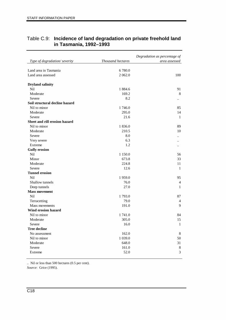
STAFF INFORMATION PAPER
C18
Table C.9: Incidence of land degradation on private freehold landin Tasmania, 1992–1993
Type of degradation/ severity Thousand hectaresDegradation as percentage of
area assessed
Land area in Tasmania 6 780.0Land area assessed 2 062.0 100
Dryland salinityNil 1 884.6 91Moderate 169.2 8Severe 8.2 ..
Soil structural decline hazardNil to minor 1 746.0 85Moderate 295.0 14Severe 21.6 1
Sheet and rill erosion hazardNil to minor 1 836.0 89Moderate 210.5 10Severe 8.0 .. Very severe 6.3 .. Extreme 1.2 ..
Gully erosionNil 1 150.0 56Minor 673.8 33Moderate 224.8 11Severe 12.6 1
Tunnel erosionNil 1 959.0 95Shallow tunnels 76.0 4Deep tunnels 27.0 1
Mass movementNil 1 793.0 87Terracetting 79.0 4Mass movements 191.0 9
Wind erosion hazardNil to minor 1 741.0 84Moderate 305.0 15Severe 16.0 1
Tree declineNo assessment 162.0 8Nil to minor 1 039.0 50Moderate 648.0 31Severe 161.0 8Extreme 52.0 3
.. Nil or less than 500 hectares (0.5 per cent).Source: Grice (1995).
APPENDIX C: THE EXTENT OF LAND DEGRADATION IN AUSTRALIA
C19
C.3 Estimates of land degradation provided in selectedpublished studies
Some specialist studies provide information about individual types of landdegradation and the rate of advance of that degradation given land managementpractices at the time. The studies are not compiled using a commonmethodology or reference periods when compared to either each other or thestate-wide studies. Therefore, the results from individual studies cannot beeasily used to prepare a national inventory of land degradation. Nevertheless,they individually provide information about land degradation that should assistin the development of an overall view of land degradation in relation to landmanagement. The approach adopted in this section is to report three officialstudies relating to irrigation salinity, dryland salinity and soil acidification —topics which are further analysed in the state-wide study of New South Walesagriculture. Other studies are available and could also be drawn upon toprovide a fuller exposition of the extent of land degradation and issues in itsmeasurement. For example: Tothill and Gillies (1992) provide a detailed studyof pasturelands in northern Australia including estimates of the extent ofvegetation decline; and Graetz et al. (1995) and the Department of theEnvironment, Sport and Territories (1995b) provide estimates of the area ofland clearance and the occurrence of selected feral animals in a study oflandcover disturbance in Australia.
Irrigation salinity
Irrigation salinity is associated with the rise in water tables as water accessionsexceed plant use and runoff. The New South Wales survey measured theseverity of salination. While not necessarily measuring the extent and severityof salination, studies have been made of changing water tables in the Murray-Darling Basin irrigation areas. These studies indicate that without interventionwater tables in the Riverine Plains Zone will continue to rise, and 30 to 50 yearprojections are provided (see Table C.10). The estimates show that the rate ofincrease in the area subject to high water tables differs between regions. In theNew South Wales irrigation areas of the Riverine Plains Zone, using thesegrowth rates, the area with high water tables could increase by around 3 per centper year during the 1990s. Because high water table areas are alreadywidespread in Victorian but less so in New South Wales, the potential increasein high water tables areas is less in Victoria (ie estimated to be below 1 per centper year during the 1990s) than in New South Wales.
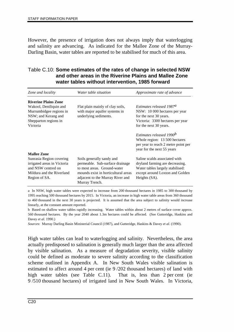
STAFF INFORMATION PAPER
C20
However, the presence of irrigation does not always imply that waterloggingand salinity are advancing. As indicated for the Mallee Zone of the Murray-Darling Basin, water tables are reported to be stabilised for much of this area.
Table C.10: Some estimates of the rates of change in selected NSWand other areas in the Riverine Plains and Mallee Zonewater tables without intervention, 1985 forward
Zone and locality Water table situation Approximate rate of advance
Riverine Plains ZoneWakool, Deniliquin andMurrumbidgee regions inNSW; and Kerang andShepparton regions inVictoria
Flat plain mainly of clay soils,with major aquifer systems inunderlying sediments.
Estimates released 1987a
NSW: 10 000 hectares per yearfor the next 30 years.Victoria: 3300 hectares per yearfor the next 30 years.
Estimates released 1990b
Whole region: 13 500 hectaresper year to reach 2 metre point peryear for the next 55 years
Mallee ZoneSunrasia Region coveringirrigated areas in Victoriaand NSW centred onMildura and the RiverlandRegion of SA.
Soils generally sandy andpermeable. Sub-surface drainageto most areas. Ground-watermounds exist in horticultural areasadjacent to the Murray River andMurray Trench.
Saline scalds associated withdryland farming are decreasing.Water tables largely stabilised:except around Loxton and GoldenHeights (SA).
a In NSW, high water tables were expected to increase from 200 thousand hectares in 1985 to 300 thousand by1995 reaching 500 thousand hectares by 2015. In Victoria, an increase in high water table areas from 360 thousandto 460 thousand in the next 30 years is projected. It is assumed that the area subject to salinity would increaselinearly, at the constant amount reported.b Based on shallow water tables rapidly increasing. Water tables within about 2 metres of surface cover approx.560 thousand hectares. By the year 2040 about 1.3m hectares could be affected. (See Gutteridge, Haskins andDavey et al. 1990.)Sources: Murray Darling Basin Ministerial Council (1987), and Gutteridge, Haskins & Davey et al. (1990).
High water tables can lead to waterlogging and salinity. Nevertheless, the areaactually predisposed to salination is generally much larger than the area affectedby visible salination. As a measure of degradation severity, visible salinitycould be defined as moderate to severe salinity according to the classificationscheme outlined in Appendix A. In New South Wales visible salination isestimated to affect around 4 per cent (ie 9 /202 thousand hectares) of land withhigh water tables (see Table C.11). That is, less than 2 per cent (ie9 /510 thousand hectares) of irrigated land in New South Wales. In Victoria,
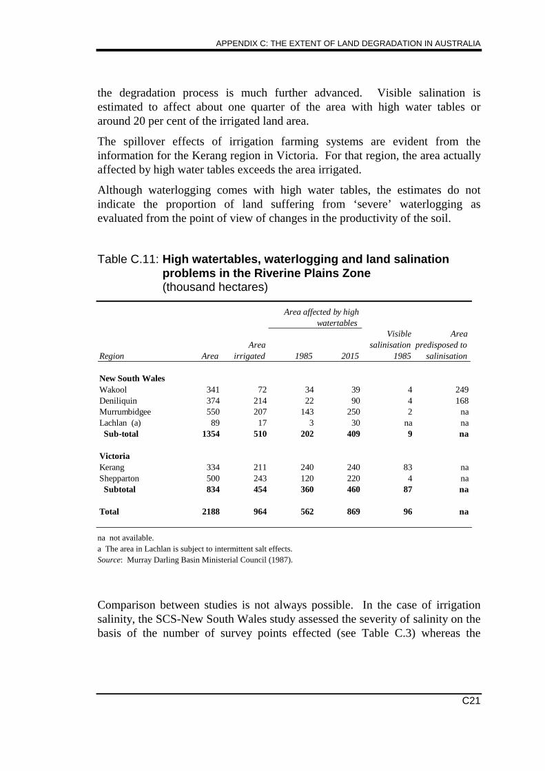
APPENDIX C: THE EXTENT OF LAND DEGRADATION IN AUSTRALIA
C21
the degradation process is much further advanced. Visible salination isestimated to affect about one quarter of the area with high water tables oraround 20 per cent of the irrigated land area.
The spillover effects of irrigation farming systems are evident from theinformation for the Kerang region in Victoria. For that region, the area actuallyaffected by high water tables exceeds the area irrigated.
Although waterlogging comes with high water tables, the estimates do notindicate the proportion of land suffering from ‘severe’ waterlogging asevaluated from the point of view of changes in the productivity of the soil.
Table C.11: High watertables, waterlogging and land salinationproblems in the Riverine Plains Zone(thousand hectares)
Area affected by highwatertables
Region AreaArea
irrigated 1985 2015
Visiblesalinisation
1985
Areapredisposed to
salinisation
New South WalesWakool 341 72 34 39 4 249Deniliquin 374 214 22 90 4 168Murrumbidgee 550 207 143 250 2 naLachlan (a) 89 17 3 30 na na Sub-total 1354 510 202 409 9 na
VictoriaKerang 334 211 240 240 83 naShepparton 500 243 120 220 4 na Subtotal 834 454 360 460 87 na
Total 2188 964 562 869 96 na
na not available.a The area in Lachlan is subject to intermittent salt effects.Source: Murray Darling Basin Ministerial Council (1987).
Comparison between studies is not always possible. In the case of irrigationsalinity, the SCS-New South Wales study assessed the severity of salinity on thebasis of the number of survey points effected (see Table C.3) whereas the
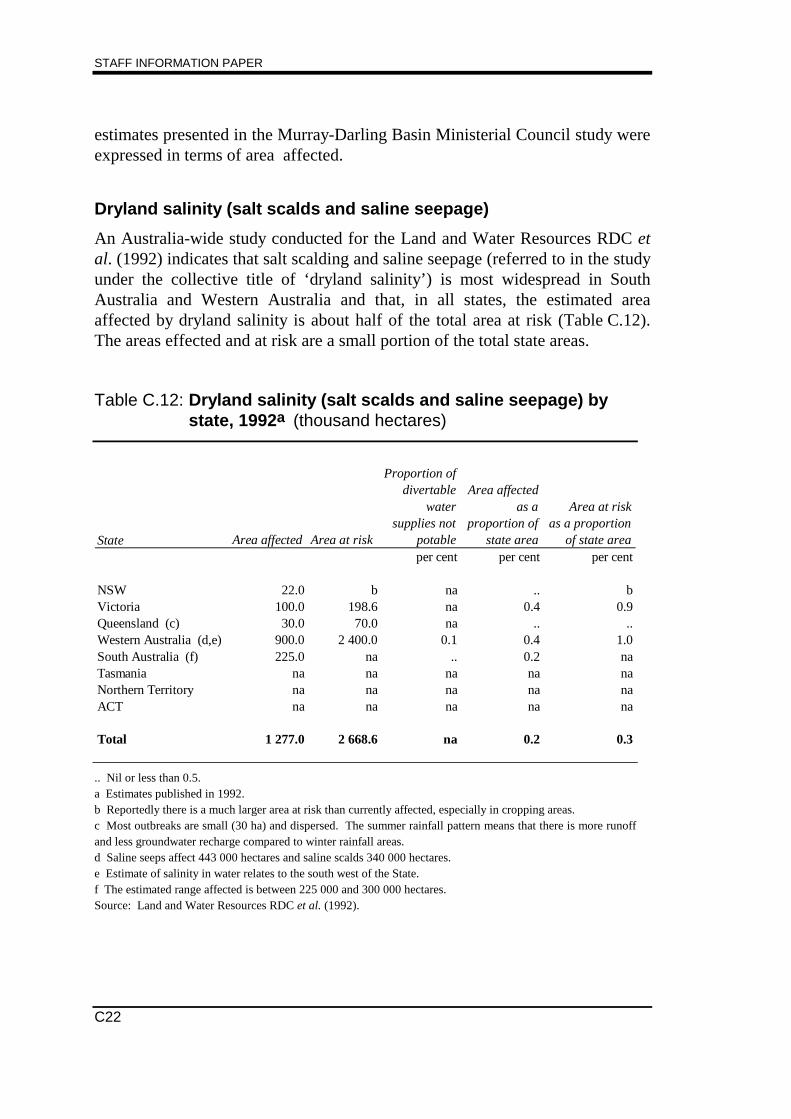
STAFF INFORMATION PAPER
C22
estimates presented in the Murray-Darling Basin Ministerial Council study wereexpressed in terms of area affected.
Dryland salinity (salt scalds and saline seepage)
An Australia-wide study conducted for the Land and Water Resources RDC etal. (1992) indicates that salt scalding and saline seepage (referred to in the studyunder the collective title of ‘dryland salinity’) is most widespread in SouthAustralia and Western Australia and that, in all states, the estimated areaaffected by dryland salinity is about half of the total area at risk (Table C.12).The areas effected and at risk are a small portion of the total state areas.
Table C.12: Dryland salinity (salt scalds and saline seepage) bystate, 1992a (thousand hectares)
State Area affected Area at risk
Proportion ofdivertable
watersupplies not
potable
Area affectedas a
proportion ofstate area
Area at riskas a proportion
of state areaper cent per cent per cent
NSW 22.0 b na .. bVictoria 100.0 198.6 na 0.4 0.9Queensland (c) 30.0 70.0 na .. ..Western Australia (d,e) 900.0 2 400.0 0.1 0.4 1.0South Australia (f) 225.0 na .. 0.2 naTasmania na na na na naNorthern Territory na na na na naACT na na na na na
Total 1 277.0 2 668.6 na 0.2 0.3
.. Nil or less than 0.5.a Estimates published in 1992.b Reportedly there is a much larger area at risk than currently affected, especially in cropping areas.c Most outbreaks are small (30 ha) and dispersed. The summer rainfall pattern means that there is more runoffand less groundwater recharge compared to winter rainfall areas.d Saline seeps affect 443 000 hectares and saline scalds 340 000 hectares.e Estimate of salinity in water relates to the south west of the State.f The estimated range affected is between 225 000 and 300 000 hectares.Source: Land and Water Resources RDC et al. (1992).
APPENDIX C: THE EXTENT OF LAND DEGRADATION IN AUSTRALIA
C23
The estimated areas affected by dryland salinity in this study differ substantiallyfrom the estimates in other studies. This may be because it is a combination oftwo forms of degradation. Induced saline seepage generally follows from landclearing and is typical of higher rainfall areas, whereas saline scalds oftenfollow from overgrazing and occur mainly in arid and semi-arid areas(Appendix A). The fact that both forms of salinity can occur naturally or beinduced by land management decisions may also contribute to the difficulty inobtaining integrated estimates from different studies.
The difference between studies is marked. In Victoria, the study indicates100 000 hectares are affected compared to the state study estimate of 135 000hectares — a one third difference. For Western Australia, the area affectedcould be as high as 900 000 hectares according to the Land and WaterResources RDC et al. (1992) review. Estimates of the components of this totalsuggest that there is 443 000 hectares of saline seepage and 340 000 hectares ofscalding — leaving a reconciliation difference of around 200 000 hectares. Theestimated saline seepage is similar to the Department of Agriculture-WesternAustralian estimate of 433 000 hectares (see Table C.8) while the estimate ofsaline scalding is not shown separately in the state departmental assessment.The area at risk in the two reports is similar.
The Land and Water Resources RDC et al. (1992) review puts the area affectedby dry land salinity in New South Wales at 22 000 hectares. The SCS–NewSouth Wales study separates saline seepages and scalding (ie dryland salinity)and surface scalds (a form of degradation typical of soil erosion in arid areas).The New South Wales study did not make area estimates for dryland salinitydue to difficulty in projecting the area affected from data collected at individualsurvey points.
In addition, for five of the states and territories, no estimates of the area at riskare provided.
Soil acidification
The extent of soil acidification was estimated as part of a Land and WaterResources RDC investigation into the amelioration of soil acidification(AACM 1995). As the survey relates to naturally acid soils rather than inducedacidification, the study does not provide a good indication of the level of landdegradation for two reasons. First, it does not show the shift due to landmanagement decisions from potentially acid soils to problem acid soils, andsecondly, it does not show any shift due to land management systems designedto improve the productivity of the land for certain crops and pastures from
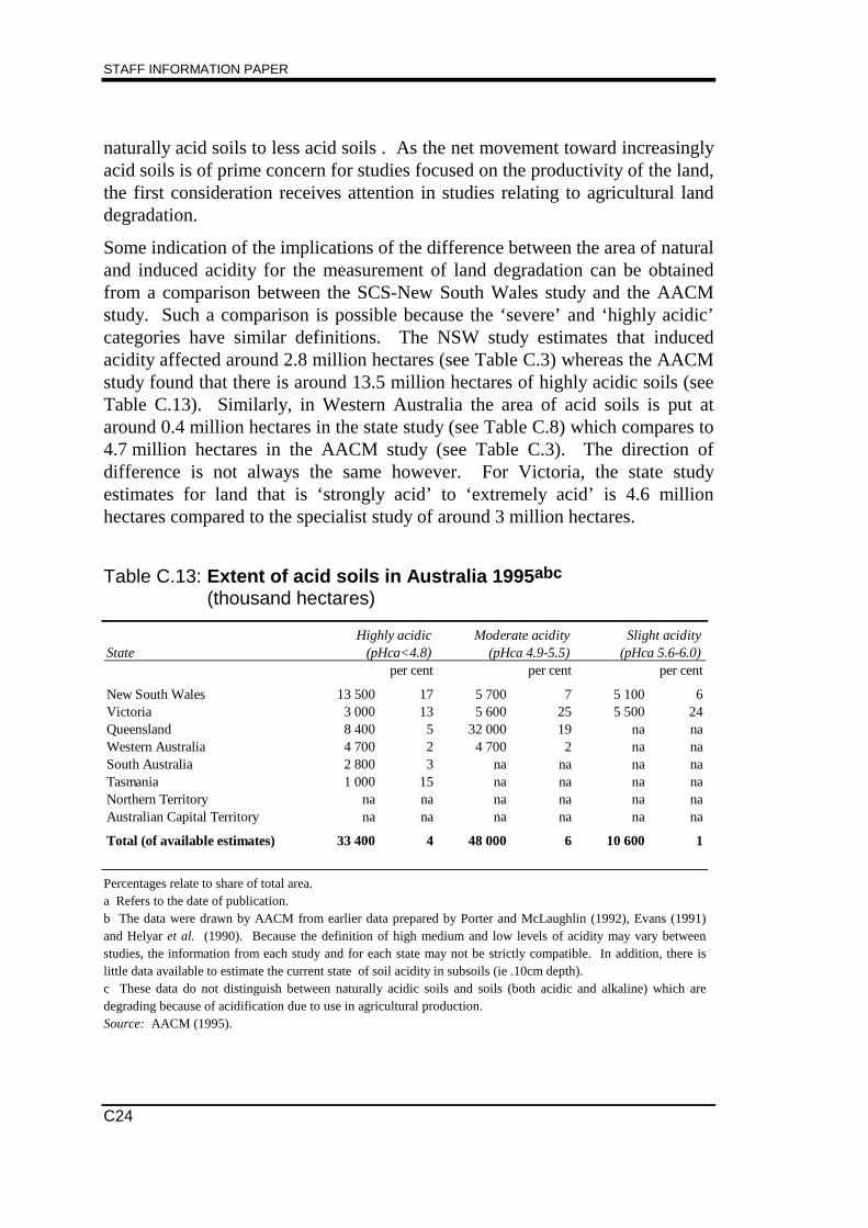
STAFF INFORMATION PAPER
C24
naturally acid soils to less acid soils . As the net movement toward increasinglyacid soils is of prime concern for studies focused on the productivity of the land,the first consideration receives attention in studies relating to agricultural landdegradation.
Some indication of the implications of the difference between the area of naturaland induced acidity for the measurement of land degradation can be obtainedfrom a comparison between the SCS-New South Wales study and the AACMstudy. Such a comparison is possible because the ‘severe’ and ‘highly acidic’categories have similar definitions. The NSW study estimates that inducedacidity affected around 2.8 million hectares (see Table C.3) whereas the AACMstudy found that there is around 13.5 million hectares of highly acidic soils (seeTable C.13). Similarly, in Western Australia the area of acid soils is put ataround 0.4 million hectares in the state study (see Table C.8) which compares to4.7 million hectares in the AACM study (see Table C.3). The direction ofdifference is not always the same however. For Victoria, the state studyestimates for land that is ‘strongly acid’ to ‘extremely acid’ is 4.6 millionhectares compared to the specialist study of around 3 million hectares.
Table C.13: Extent of acid soils in Australia 1995abc
(thousand hectares)
Highly acidic Moderate acidity Slight acidityState (pHca<4.8) (pHca 4.9-5.5) (pHca 5.6-6.0)
per cent per cent per cent
New South Wales 13 500 17 5 700 7 5 100 6Victoria 3 000 13 5 600 25 5 500 24Queensland 8 400 5 32 000 19 na naWestern Australia 4 700 2 4 700 2 na naSouth Australia 2 800 3 na na na naTasmania 1 000 15 na na na naNorthern Territory na na na na na naAustralian Capital Territory na na na na na na
Total (of available estimates) 33 400 4 48 000 6 10 600 1
Percentages relate to share of total area.a Refers to the date of publication.b The data were drawn by AACM from earlier data prepared by Porter and McLaughlin (1992), Evans (1991)and Helyar et al. (1990). Because the definition of high medium and low levels of acidity may vary betweenstudies, the information from each study and for each state may not be strictly compatible. In addition, there islittle data available to estimate the current state of soil acidity in subsoils (ie .10cm depth).c These data do not distinguish between naturally acidic soils and soils (both acidic and alkaline) which aredegrading because of acidification due to use in agricultural production.Source: AACM (1995).
APPENDIX C: THE EXTENT OF LAND DEGRADATION IN AUSTRALIA
C25
Overall, New South Wales is reported as having the largest part of its surfacearea subject to highly acid soils, followed by Tasmania. In addition, slightlyacid and moderately acid soils predominate in Victoria and Queensland.
Degradation in this study is concerned with changing levels of soil acidificationdue principally to agricultural use. Concerning the advance of soil acidification,the AACM study indicates that:
• higher rainfall areas in south western and eastern Australia have thehighest risk of soil acidification;
• more than 55 million hectares of moderately or slightly acidic land (pHCa4.9–6.0) across Australia have the potential to degrade to highly acidicconditions (pHCa <4.8);
• many soils in north east Victoria have acidified by 1 pH unit during thelast 30 to 40 years; and
• modest rates of acidification in New South Wales will result in subsurfaceacidification of 1 pH unit within 23 years for sandy soils and 113 years forclay soils.
In order to provide indicative measures of the possible rate of advance ofacidification, with no change in soil management, the advances reported inpoints three and four in the previous paragraph, are calibrated to a (hypothetical)one fifth increase from a slightly to moderately acidic base, over the periodmentioned for each region.2 The indicative rates of advance calculated on thatbasis are:
• 0.5 percentage points each year for north eastern Victoria for the last fortyyears;
• 1 percentage point each year for the next 20 years for sandy soils in NSW;and
• 0.2 percentage point each year for the next 110 years for clay soils inNSW.
2 One fifth (ie 0.2) is estimated as 1pH over a base of 5.5 pH which is the average of the
range of moderate to slight acidity as reported in Table C.13. The percentage points
change in acidity from a base of 5.5=100 is therefore given by 1
5 5
100 0 2100
.*
.*
yrs yrs≈
where yrs refers to the number of years over which the expected acidification is forecast tooccur. For example, the percentage points change in acidification over the last 40 years in
Victoria is given by 1
5 5
100
400 5
.* .≈ per annum.
STAFF INFORMATION PAPER
C26
These projections indicate that the annual rate of change is sensitive to soiltypes and that even for the soils most vulnerable, the rate of degradation mayappear slow. Although induced acidity may be farm specific, identifying theeffects of degradation on farm productivity and managing appropriateamelioration strategies may be difficult.
D1
APPENDIX DCONCEPTUAL MODEL OF LANDDEGRADATION, FARM OUTPUT AND PROFITS
D.1 Introduction
From the point of view of agricultural land use, most land resources subject todegradation are renewable either through human conservation efforts or naturalprocesses (see Appendix A). While topsoil is normally regarded as a non-renewable resource, its vulnerability to soil erosion (or soil erosion hazard) dueto the action of wind and water can be reduced through conservation efforts.
Sustainable land use in agriculture is therefore a two way process. On one hand,there is a loss of productivity as land resources are used up in currentproduction, while, on the other, conservation expenditure and naturalregeneration can renew those resources and improve productivity for future use.This appendix uses a stylised model of natural resource use to consider thesalient features of this two way process. It is also used to consider how the bio-physical process of land degradation and conservation inter-relate with farmoutputs and profits. A more formal presentation of the basic ideas considered inthis appendix can be found in studies by Clarke (1992), Sweeney (1993) andPagiola (1993) while the presentation used to develop this discussion of landdegradation is adapted from Pearce and Turner (1990).
In principle, there are many levels of land resource use, conservation effort anddegradation consistent with the profitable operation of farming enterprises andsustainability of the agricultural industry. The principles, however, do notprovide prescriptions concerning what those levels should be. That is anempirical question which is considered in other parts of this information paper.
Section D.2 sets out a typical pattern of regeneration of the land condition andfertility following some process of land degradation while Section D.3 linksagricultural activity to changes in land condition and fertility. Distinctions aremade between exploitative and conservation effort, and natural regeneration.Section D.4 places a cost on exploitation effort and Section D.5 discussespossible production outcomes from farmer effort and from the use of landresources in various stages of degradation. Section D.6 then links thediscussion of agricultural revenues and costs to define profits from land use, andthe limits likely to be placed on degradation by standard commercial incentives
STAFF INFORMATION PAPER
D2
to maximise profits. The framework discussion provided in Sections D.2 to D.6is placed in a broader environmental and economic context in Section D.7which considers some of the simplifying assumptions of the stylised model andsome general ecological issues that are not necessarily taken into account inagricultural land management decisions. Section D.8 provides a summary.
D.2 Typical pattern in the regeneration of land resources
The processes of land use and regeneration move forward in time and at anypoint in that continuum, land condition and fertility can be represented as somestock which has value for human or environmental use. The condition of theland does not stand still even without human intervention. Nevertheless, it isgenerally agreed that the intensive use of land by humans speeds and modifiesthe processes of change. This means that there is a requirement forconservation effort if the productivity of the land is to be maintained for futureuse.
In this dynamic context, sustainability of agriculture requires the maintenance ofthe productive capacity of land through time; with the farmer setting out toachieve some economic yield over the years. However, there are both bio-physical forces and economic imperatives at work so that the farmer does notface a static situation. The difficulty with defining a framework for evaluatingthe potential for sustainability is therefore in linking the bio-physical process ofland use with the economic processes that determine the incentives for that use.A useful starting point is the regeneration potential of land condition and itsfertility. This starting point establishes a reference against which the resourceusing effects of agricultural production can be related to the regeneration effectsof conservation and natural processes.
The regeneration potential of land resources are likely to differ depending onthe prevailing condition of the land, with regeneration processes being slowwith highly degraded land. As land conditions improve, the potential for furtherimprovements in condition and fertility as natural processes begin to replacenutrients and chemical, repair soil structure etc, would also improve (seeFigure D.1a). This process could continue until, at the other end of thespectrum, the land resource reaches its potential fertility level and the scope forfurther improvement no longer exists.
By evaluating the expected improvement in land condition and fertility for eachresource level, it is possible to define the rate of regeneration that would occurwith the elapse of time (Figure D.1b). The rate of regeneration so determined isagain depicted as being smallest when the land condition and fertility levels are
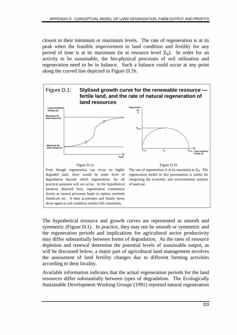
APPENDIX D: CONCEPTUAL MODEL OF LAND DEGRADATION, FARM OUTPUT AND PROFITS
D3
closest to their minimum or maximum levels. The rate of regeneration is at itspeak when the feasible improvement in land condition and fertility for anyperiod of time is at its maximum (ie at resource level Z0). In order for anactivity to be sustainable, the bio-physical processes of soil utilisation andregeneration need to be in balance. Such a balance could occur at any pointalong the curved line depicted in Figure D.1b.
Figure D.1: Stylised growth curve for the renewable resource —fertile land, and the rate of natural regeneration ofland resources
Maximum forland resources
Minimum forland resources
Time
Land condition/fertility (Z)
Regeneration
Zmin
Rmax
ZmaxZ0 Land condition/
fertility (Z)
dZ
dt
Figure D.1aEven though regeneration can occur on highlydegraded land, there would be some level ofdegradation beyond which regeneration, for allpractical purposes will not occur. In the hypotheticalsituation depicted here, regeneration commencesslowly as natural processes begin to replace nutrientschemicals etc. It then accelerates and finally slowsdown again as soil condition reaches full restoration.
Figure D.1bThe rate of regeneration is at its maximum at Z0. Theregeneration model in this presentation is useful forintegrating the economic and environmental analysisof land use.
The hypothetical resource and growth curves are represented as smooth andsymmetric (Figure D.1). In practice, they may not be smooth or symmetric andthe regeneration periods and implications for agricultural sector productivitymay differ substantially between forms of degradation. As the rates of resourcedepletion and renewal determine the potential levels of sustainable output, aswill be discussed below, a major part of agricultural land management involvesthe assessment of land fertility changes due to different farming activitiesaccording to their locality.
Available information indicates that the actual regeneration periods for the landresources differ substantially between types of degradation. The EcologicallySustainable Development Working Groups (1991) reported natural regeneration
STAFF INFORMATION PAPER
D4
periods ranging from around five years for forms of degradation relating to soilnutrient exhaustion and induced top soil acidity to periods approaching100 years for water logging and salinity. These periods relate to bio-physicalprocesses and do not capture the nature or direction of changes in agriculturalsector productivity or profitability. While loss of topsoil is treated as apermanent loss of land resources by the Working Group, the vulnerability of theland to erosion and, through this, topsoil loss, can be treated as a renewableresource within the framework being outlined.
D.3 The link between agricultural land use and changes inland resources
In order to maintain a sustainable system of agriculture (for a given technology),it would be necessary for the use of land resources to be matched by the rate ofregeneration. Where this matching occurs there will be a steady state that issustainable. The curve showing fertility yielded (a flow measure) against landcondition/fertility (a measure of the resource stock) depicts all those points atwhich yield matches regeneration (see Figure D.2). Each of those points issustainable in a steady state. However, there is only one combination ofresource yield (say in the production of wheat) and land resource stocks that isconsistent with a steady state maximum sustainable land resource use. Thisoccurs at the point when the regeneration capability of the land is at itsmaximum. The soil condition and fertility level associated with the maximumsustainable yield (or renewable resource use) is depicted by Z2 with potentialyield being Y2 in Figure D.2.
Use of the land resource to obtain some yield from the soil involves effort onthe part of the farmer through the commitment of labour and the deployment ofcapital equipment and materials. The yield obtained by the farmer is thereforejointly determined by his or her effort and the condition of the soil. Figure D.2depicts how the choice of effort level will determine both yield and resourcestock level. It does this by showing yield as a function of effort (E) andresource stocks (Z), that is Y f E Zn= ( , ) . In this set up, the level of effort E ischosen by the farmer, while yield and the resource stock vary according to thatchoice.
The agricultural industry effort necessary in this set up to obtain maximumsustainable yield is level E2 (Figure D.2). With this amount of effort, yield andresource stock levels adjust so that yield equals the highest possible level ofregeneration. This is depicted in Figure D.2 by the intersection of the yield linewith the land regeneration curve. Effort level E2 could also be committed when
APPENDIX D: CONCEPTUAL MODEL OF LAND DEGRADATION, FARM OUTPUT AND PROFITS
D5
the land has higher (towards Zmax) or lower (towards Zmin) levels of fertility togive differing yields. However, with those effort-resource combinations,regeneration and yield would not coincide and the resource stock would beeither increasing or declining, depending on the circumstances. For example, ifland condition and fertility were above Z2, the level of effort being appliedwould cause resources to be used at a rate above that at which they couldregenerate and there would be a net depletion of the resource stock. On theother hand, if the land condition and fertility level were below Z2, the amount ofeffort would cause the resource stock to be used at a rate below that at which itcould regenerate, and there would be a net addition to the resource stock.
Maximum sustainable resource yield is only one of many different possiblelevels of yield. However, the other possible sustainable yields would beassociated with a different levels of land condition and farmer effort. Forexample, an hypothetical increase in farmer effort — depicted as a shift of effortfrom level E2 to a higher level of effort E3 — could initially yield a temporaryincrease in production as the resource stock was mined. However, becauseregeneration could not keep up with the resource depletion brought about by theadditional effort, the natural resource stock would decline. Providingexploitative effort did not change, a new point on the regeneration/yield curvewould be reached where the resources yielded would be again matched by therate of regeneration. However, in the case depicted in Figure D.2, the newhigher level of effort sustains lower yields.
In agriculture, higher levels of effort may be reflected in higher harvesting costsper unit of output as the crop quality and pasture yields decline withdeteriorating land condition and fertility (ie as the resource stock moves towardZmin in the analytical framework depicted in Figure D.2). For livestock, higheranimal husbandry and mustering costs per animal are likely as animals aregrazed on larger areas due to declining pasture quality that comes withdegradation.
If farmer effort is reduced (eg from E2 to E1), the exploitative use of the landwould decrease and land condition and fertility would increase to Z1.
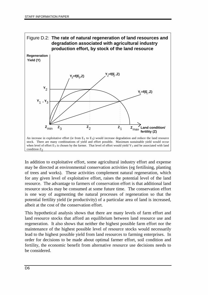
STAFF INFORMATION PAPER
D6
Figure D.2: The rate of natural regeneration of land resources anddegradation associated with agricultural industryproduction effort, by stock of the land resource
1
Y2
Z2 Zmax
Yield (Y)
Zmin Z1
Y =f(E ,Z) 3
1Y
Z3 Land condition/fertility (Z)
Regeneration
Y =f(E ,Z)
Y =f(E ,Z) 2
3, Y
32
1
An increase in exploitative effort (ie from E1 to E3) would increase degradation and reduce the land resourcestock. There are many combinations of yield and effort possible. Maximum sustainable yield would occurwhen level of effort E2 is chosen by the farmer. That level of effort would yield Y2 and be associated with landcondition Z2
In addition to exploitative effort, some agricultural industry effort and expensemay be directed at environmental conservation activities (eg fertilising, plantingof trees and works). These activities complement natural regeneration, whichfor any given level of exploitative effort, raises the potential level of the landresource. The advantage to farmers of conservation effort is that additional landresource stocks may be consumed at some future time. The conservation effortis one way of augmenting the natural processes of regeneration so that thepotential fertility yield (ie productivity) of a particular area of land is increased,albeit at the cost of the conservation effort.
This hypothetical analysis shows that there are many levels of farm effort andland resource stocks that afford an equilibrium between land resource use andregeneration. It also shows that neither the highest possible farm effort nor themaintenance of the highest possible level of resource stocks would necessarilylead to the highest possible yield from land resources to farming enterprises. Inorder for decisions to be made about optimal farmer effort, soil condition andfertility, the economic benefit from alternative resource use decisions needs tobe considered.
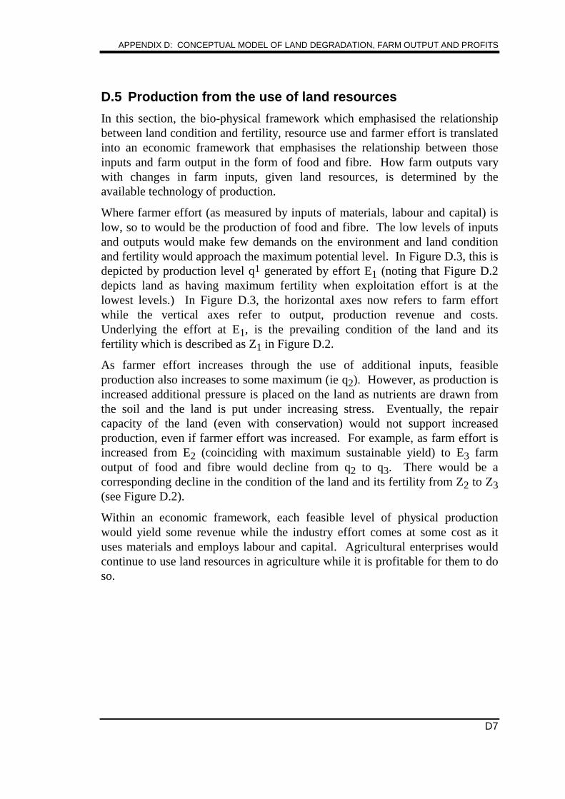
APPENDIX D: CONCEPTUAL MODEL OF LAND DEGRADATION, FARM OUTPUT AND PROFITS
D7
D.5 Production from the use of land resources
In this section, the bio-physical framework which emphasised the relationshipbetween land condition and fertility, resource use and farmer effort is translatedinto an economic framework that emphasises the relationship between thoseinputs and farm output in the form of food and fibre. How farm outputs varywith changes in farm inputs, given land resources, is determined by theavailable technology of production.
Where farmer effort (as measured by inputs of materials, labour and capital) islow, so to would be the production of food and fibre. The low levels of inputsand outputs would make few demands on the environment and land conditionand fertility would approach the maximum potential level. In Figure D.3, this isdepicted by production level q1 generated by effort E1 (noting that Figure D.2depicts land as having maximum fertility when exploitation effort is at thelowest levels.) In Figure D.3, the horizontal axes now refers to farm effortwhile the vertical axes refer to output, production revenue and costs.Underlying the effort at E1, is the prevailing condition of the land and itsfertility which is described as Z1 in Figure D.2.
As farmer effort increases through the use of additional inputs, feasibleproduction also increases to some maximum (ie q2). However, as production isincreased additional pressure is placed on the land as nutrients are drawn fromthe soil and the land is put under increasing stress. Eventually, the repaircapacity of the land (even with conservation) would not support increasedproduction, even if farmer effort was increased. For example, as farm effort isincreased from E2 (coinciding with maximum sustainable yield) to E3 farmoutput of food and fibre would decline from q2 to q3. There would be acorresponding decline in the condition of the land and its fertility from Z2 to Z3(see Figure D.2).
Within an economic framework, each feasible level of physical productionwould yield some revenue while the industry effort comes at some cost as ituses materials and employs labour and capital. Agricultural enterprises wouldcontinue to use land resources in agriculture while it is profitable for them to doso.
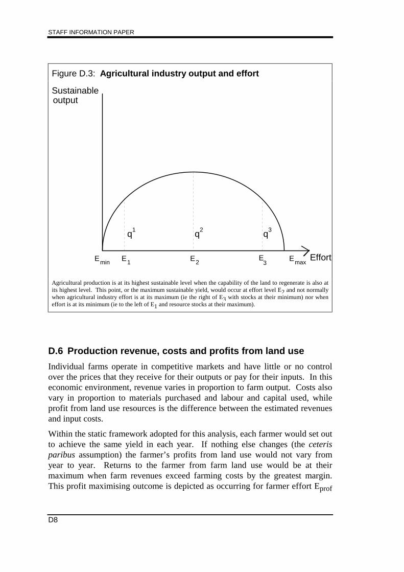
STAFF INFORMATION PAPER
D8
Figure D.3: Agricultural industry output and effort
EffortE 2E 1
q1
E 3
q2 q3
E maxminE
outputSustainable
Agricultural production is at its highest sustainable level when the capability of the land to regenerate is also atits highest level. This point, or the maximum sustainable yield, would occur at effort level E2 and not normallywhen agricultural industry effort is at its maximum (ie the right of E3 with stocks at their minimum) nor wheneffort is at its minimum (ie to the left of E1 and resource stocks at their maximum).
D.6 Production revenue, costs and profits from land use
Individual farms operate in competitive markets and have little or no controlover the prices that they receive for their outputs or pay for their inputs. In thiseconomic environment, revenue varies in proportion to farm output. Costs alsovary in proportion to materials purchased and labour and capital used, whileprofit from land use resources is the difference between the estimated revenuesand input costs.
Within the static framework adopted for this analysis, each farmer would set outto achieve the same yield in each year. If nothing else changes (the ceterisparibus assumption) the farmer’s profits from land use would not vary fromyear to year. Returns to the farmer from farm land use would be at theirmaximum when farm revenues exceed farming costs by the greatest margin.This profit maximising outcome is depicted as occurring for farmer effort Eprof
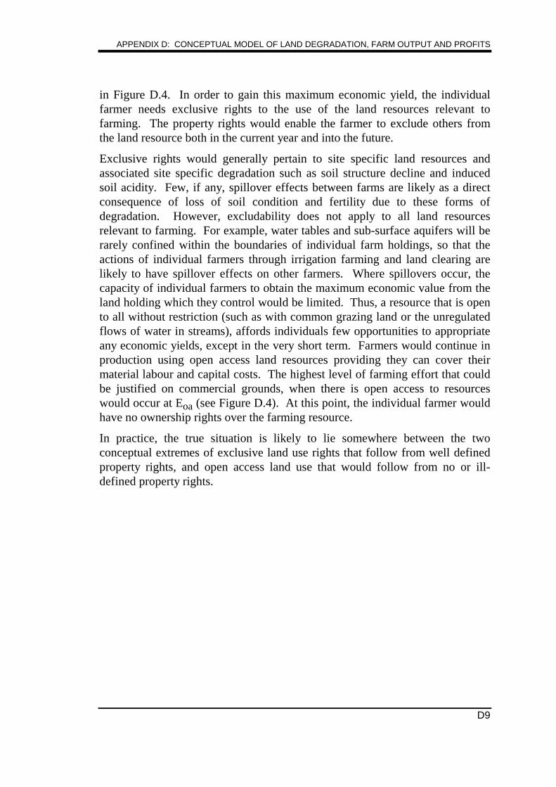
APPENDIX D: CONCEPTUAL MODEL OF LAND DEGRADATION, FARM OUTPUT AND PROFITS
D9
in Figure D.4. In order to gain this maximum economic yield, the individualfarmer needs exclusive rights to the use of the land resources relevant tofarming. The property rights would enable the farmer to exclude others fromthe land resource both in the current year and into the future.
Exclusive rights would generally pertain to site specific land resources andassociated site specific degradation such as soil structure decline and inducedsoil acidity. Few, if any, spillover effects between farms are likely as a directconsequence of loss of soil condition and fertility due to these forms ofdegradation. However, excludability does not apply to all land resourcesrelevant to farming. For example, water tables and sub-surface aquifers will berarely confined within the boundaries of individual farm holdings, so that theactions of individual farmers through irrigation farming and land clearing arelikely to have spillover effects on other farmers. Where spillovers occur, thecapacity of individual farmers to obtain the maximum economic value from theland holding which they control would be limited. Thus, a resource that is opento all without restriction (such as with common grazing land or the unregulatedflows of water in streams), affords individuals few opportunities to appropriateany economic yields, except in the very short term. Farmers would continue inproduction using open access land resources providing they can cover theirmaterial labour and capital costs. The highest level of farming effort that couldbe justified on commercial grounds, when there is open access to resourceswould occur at Eoa (see Figure D.4). At this point, the individual farmer wouldhave no ownership rights over the farming resource.
In practice, the true situation is likely to lie somewhere between the twoconceptual extremes of exclusive land use rights that follow from well definedproperty rights, and open access land use that would follow from no or ill-defined property rights.
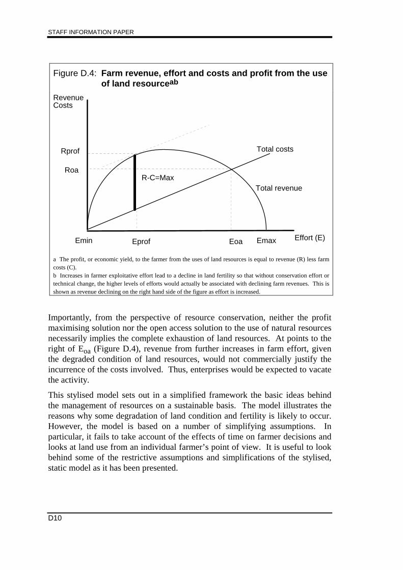
STAFF INFORMATION PAPER
D10
Figure D.4: Farm revenue, effort and costs and profit from the useof land resourceab
R-C=Max
RevenueCosts
Effort (E)
Total costs
Eprof Eoa Emax
Total revenue
Rprof
Roa
Emin
a The profit, or economic yield, to the farmer from the uses of land resources is equal to revenue (R) less farmcosts (C).b Increases in farmer exploitative effort lead to a decline in land fertility so that without conservation effort ortechnical change, the higher levels of efforts would actually be associated with declining farm revenues. This isshown as revenue declining on the right hand side of the figure as effort is increased.
Importantly, from the perspective of resource conservation, neither the profitmaximising solution nor the open access solution to the use of natural resourcesnecessarily implies the complete exhaustion of land resources. At points to theright of Eoa (Figure D.4), revenue from further increases in farm effort, giventhe degraded condition of land resources, would not commercially justify theincurrence of the costs involved. Thus, enterprises would be expected to vacatethe activity.
This stylised model sets out in a simplified framework the basic ideas behindthe management of resources on a sustainable basis. The model illustrates thereasons why some degradation of land condition and fertility is likely to occur.However, the model is based on a number of simplifying assumptions. Inparticular, it fails to take account of the effects of time on farmer decisions andlooks at land use from an individual farmer’s point of view. It is useful to lookbehind some of the restrictive assumptions and simplifications of the stylised,static model as it has been presented.
APPENDIX D: CONCEPTUAL MODEL OF LAND DEGRADATION, FARM OUTPUT AND PROFITS
D11
D.7 Some broader implications of agricultural land use
In a dynamic context, the sustainability of agriculture requires the maintenanceof the productive capacity of the land through time. The availability ofinformation to the individual farmer about the process of degradation, theeffects of discounting, and the availability of alternative land uses, mean that thesimplified model does not capture all of the dynamic changes that effectagriculture.
Degradation is a dynamic process with the rate of change in the condition of theland and its fertility being the result of past farming decisions taken over manyyears. Because the process of degradation is generally regarded as being slow,its effects on farm productivity may only emerge gradually. They would also beintermingled with the effects of other changes such as the weather andtechnology over which individual farmers have little or no control. As part ofthis dynamic process, the forms of degradation may also change so that therecan be lags between the incidence of degradation, initial recognition and thedevelopment of conservation strategies. The degradation problems of onegeneration may have been the solution to previous problems or efforts toimprove farm productivity (eg induced soil acidity is associated with theintroduction of improved subterranean clover pastures and the use ofsuperphosphate and ammonium fertilisers intended to stabilise topsoil andimprove productivity). Farmers may not always be in possession of all theinformation needed to maximise economic yields from land resources.
Discounting is used to capture both social and private time preferences and isrelevant to the assessment of degradation and its effects which are spread overmany years. As social and private discount rates are usually positive, the effectof discounting would lead farmers and the community to value currentproduction above future production. In doing this, private and social discountrates would raise agricultural industry effort above the level that would providethe static maximum sustainable economic yield occurring at Eprof (seeFigure D.4). The static model, therefore, implicitly assumes that the farmers’discount rate is zero with farmers giving equal weight to present and futurereturns. On the other hand, if farmers give little weight to income from land usein the future, they would tend to give little value to the future productivecapacity of the land and would expand production so that only current material,labour and capital costs are covered (ie the open access outcome in the staticmodel). Traditionally, social discount rates are deemed to be lower than privatediscount rates, indicating that, all other things being equal, the communitywould give higher weight to resource conservation for some future use thanindividual farmers.
STAFF INFORMATION PAPER
D12
Because prevailing discount rates are neither zero or approaching infinity (ievery large), the actual land resource use outcome would fall between the twoextremes indicated by the static model. In broad terms, a farming activity wouldonly be sustainable from a farmer point of view if the rate of regeneration ofland resources used in agriculture was at least equal to the prevailing privatediscount rate.
The model as depicted in this appendix only refers to a single commodity andproduction technology. In practice, farmers may be able to choose between anumber of farming activities that are suited to a locality. They may also be ableto choose between continuing farming in the locality or vacating the land to analternative use (such as housing, mining or secondary industry). A farmingactivity would only be sustainable if the present value of its returns were: (i)positive; and (ii) higher than alternative activities not requiring the conservationof the land’s productive capacity through time (Pagiola 1993).
From the perspective of the general ecology of farming regions (includingnatural ecological systems), the stylised model does not address all potentialconcerns. In the model, the productivity of land resources is considered fromthe perspective of their use for the production of food and fibre. Where thereare natural ecological systems that require preservation to satisfy othercommunity needs and depend on land resources not necessary for farming, theirvaluation for farming could be below that of the community. Non-agriculturaluses that could be given a high value include the use of landscapes as habitatsfor native species, water catchments and areas of scenic beauty.
D.8 Summing up
The bio-physical processes of agricultural land use and land degradation can belinked conceptually to commercial incentives faced by farmers. At a conceptuallevel, this framework illustrates that with freedom of entry to and exit from thefarming industry, farming decisions based on purely commercial grounds willnot lead to the total degradation of land resources relevant to farming.
However, farming activities rival traditional ecosystems for the use of allresources within the landscape, and clearly any commercial incentives topreserve all aspects of the landscape are likely to be only incidental to farmingdecisions. Modification of the landscape to suit farming enterprises, even ifsustainable from a farming point of view, could exclude pre-farming ecosystemsof a region. Decisions based on achieving the highest level of farm enterpriseprofits will therefore not necessarily provide the same outcomes as decisionsbased on community values that take into account other land uses including the

APPENDIX D: CONCEPTUAL MODEL OF LAND DEGRADATION, FARM OUTPUT AND PROFITS
D13
preservation of traditional ecologies, natural landscapes, residentialdevelopment and the growth of mining and secondary industries.

E1
APPENDIX EPRODUCTION EQUIVALENT OF DEGRADATION,AND COSTS AND BENEFITS OF AMELIORATION
E.1 Introduction
Implicit in the concept of land degradation is the notion that agricultural landuse removes something from the soil. Without natural regeneration or landmanagement, the productivity of the land would be reduced. Appendix Eoutlines economic concepts which show that levels of production, profit anddegradation are linked and that because of these links, a balance exists betweenincreasing production and allowing more degradation.
Estimates of production lost from degradation and the costs and benefits ofamelioration provide information that illustrates the trade-off between higherproduction and degradation.
The level of degradation can simply be reported as lost productivity (ie a cost).One benchmark against which lost productivity could be assessed would bepotential productivity of the land, without degradation, in its current use. Thisstatic concept is useful in translating bio-physical measures of degradation intoa standardised numeraire, that is, dollars of production or net revenues. Theproduction equivalent measure does not, however, provide an estimate of thecost of achieving a benchmark level of production or indeed, the practicabilityof reaching such a target. For example, a zero degradation measure might onlybe achievable by retiring land from its current use (eg reverting from irrigationfarming to dry land farming to ameliorate irrigation salinity). Alternatively, itmight be achieved through soil treatment programs (eg liming problem acidsoils).
Cost-benefit studies of land management and amelioration possibilities are moreforward looking and are undertaken to examine the feasibility of repair andconservation efforts under various plausible options of land management. Cost-benefit studies provide an account of expected future costs and benefits of aland management or amelioration project in current period values through aprocess of discounting. The benchmark for such an analysis would be noamelioration project. A cost-benefit approach is therefore concerned with gainsfrom future repair and conservation actions.
STAFF INFORMATION PAPER
E2
Degradation amelioration actions, however, may represent only one investmentchoice available to individual land managers to improve farm productivity.Thus, even though a cost-benefit study may show positive returns to anamelioration project against the without-project benchmark, there may be otherprojects available to the farming community that afford even higher gains. Inchoosing between alternative projects, investors would be expected to assess therelative gains available from individual projects in the context of budgetconstraints that they may face. The focus of cost-benefit studies considered inthis appendix is on the expected returns from amelioration projects
This appendix first discusses the concept of the production equivalent ofdegradation and reports selected studies based on this concept (section E.2).Section E.3 discusses some general issues concerning cost-benefit analysis, andconsiders a selection of cost-benefit studies of degradation ameliorationpossibilities. Section E.3 provides a summary of the appendix.
E.2 Static measures of land degradation
Conceptual framework
In order to take a snapshot of degradation and report its severity according to acommon unit of measurement that is readily related to other informationentering into economic management decisions, the level of degradation cansimply be reported as a reduction in the potential agricultural productivity of theland. Such a measure would give degradation an economic meaning that is notdirectly possible through index measures as presented in Appendix C.
One benchmark against which reduced agricultural productivity could beassessed would be potential production using agricultural land, withoutdegradation, in its current use (or likely use if the land is unused). This conceptis useful in translating a measure of the incidence of degradation into astandardised numeraire, that is dollars of production or net revenues. Ameasure based on this concept with respect to production, could be referred toas the production equivalent of degradation. It would be a static measure of thefinancial value of degradation that could be evaluated by assuming competitivemarkets, thus:
(i) the output of each agricultural holding or locality subject to degradation istoo small to influence the price it receives for its produce. In other words,each locality faces infinite elasticities of demand or input supply;
APPENDIX E: PRODUCTION EQUIVALENT OF DEGRADATION AND COSTS AND BENEFITS OFAMELIORATION
E3
(ii) the land is assessed to be predominantly used for agriculture, either in thedegraded state or after the amelioration of degradation;
(iii) the composition of agricultural output in the absence of degradation can beassessed and the appropriate benchmark price for outputs is the currentdomestic market price (reflecting the import substitution or export parityprice for traded produce or the domestic market price for non-tradedproduce); and
(iv) in the absence of degradation, the price of agricultural outputs and goods,services and factors used in production represents the opportunity cost tothe community. This would imply that there are no price or quantitydistortions other than those included in the analysis.
Estimates of the production equivalent of degradation are normally providedwith respect to the negative effects of land modification on agriculturalproduction (eg reported production costs/losses or deviations from potentialoutput). In interpreting such measures, it should be recalled that theenvironment is also modified to improve agricultural productivity, for example,through the clearance of land and native vegetation replacement. Thesemodifications could be deemed as degradation from another perspective,although the cost of such degradation would not be within the scope ofconventional production equivalent measures.
Measures of the production equivalent of degradation that are reported, fromtime to time using the above assumptions (or are loosely based on thoseassumptions) provide broad indicators of the extent of degradation according toa common numeraire. However, they are not true costs of degradation becausethe assumptions ignore benefits that have accrued to the community from pastagricultural production, and the fact that some types of degradation occur as aresult of more productive farming systems. The potential production used as abenchmark also may not be a sustainable or optimal measure when evaluatedagainst economic criteria discussed in Appendix E. The measures therefore donot take into account the key processes and farm decisions that lead todegradation or the land management decisions arising from land degradation.For example, the measures do not take into account:

STAFF INFORMATION PAPER
E4
• the extent to which degradation is compensated by previous income flowsfrom agricultural land use which have provided incentives for degradation.For example, the clearance of land for agriculture, soil structure decline,induced soil acidity and some dryland salinity each represent a form ofland degradation that has been used to produce income from pastactivities;
• the extent to which degradation is uncompensated by previous incomeflows. This occurs when the form of degradation is invasive and hasarisen without the compensating benefits of higher production in thelocality experiencing the degradation. For example, invasion by pestanimals, plants and insects and some cases of irrigation and drylandsalinity and induced river pollution;
• off-site effects or externalities, for example, induced irrigation and drylandsalinity or river pollution occurring remotely from the farming activitiesgiving rise to those forms of degradation;
• the relationship between degradation and other factors affectingagricultural productivity such as the use of heavy machinery, supply ofwater in irrigation areas, cultivation of selected pastures and crops and thetolerance of differing farming systems to different forms of degradation;
• the cost of amelioration or management of the form of degradation; and
• the prospects of substitution between different agricultural land usesemploying current technology and the prospects for technological change.For example, the substitution of salt tolerant for salt sensitive crops, theadoption of more water efficient farm management practices in irrigationareas and the research and development of more acid tolerant farm crops.
Results from selected studies
There is a developing history of the estimation and reporting of productionequivalents of degradation. The format and coverage of these estimates differ.This section reports the results of a selection of studies.
From time to time national overview estimates of the production equivalent ofdegradation are reported. For example, in a recent overview publication, theDepartment of Environment, Sport and Territories estimated that landdegradation cost $1.15 billion annually in lost production (DEST 1995) which isaround 5 per cent of the local value of agricultural production of $23.4 billion in1994–95 (ABS Cat. No. 5206.0). A recent Prime Ministerial statement put theproduction equivalent of degradation at around 6 per cent of agriculturalproduction or about $1.5 billion.
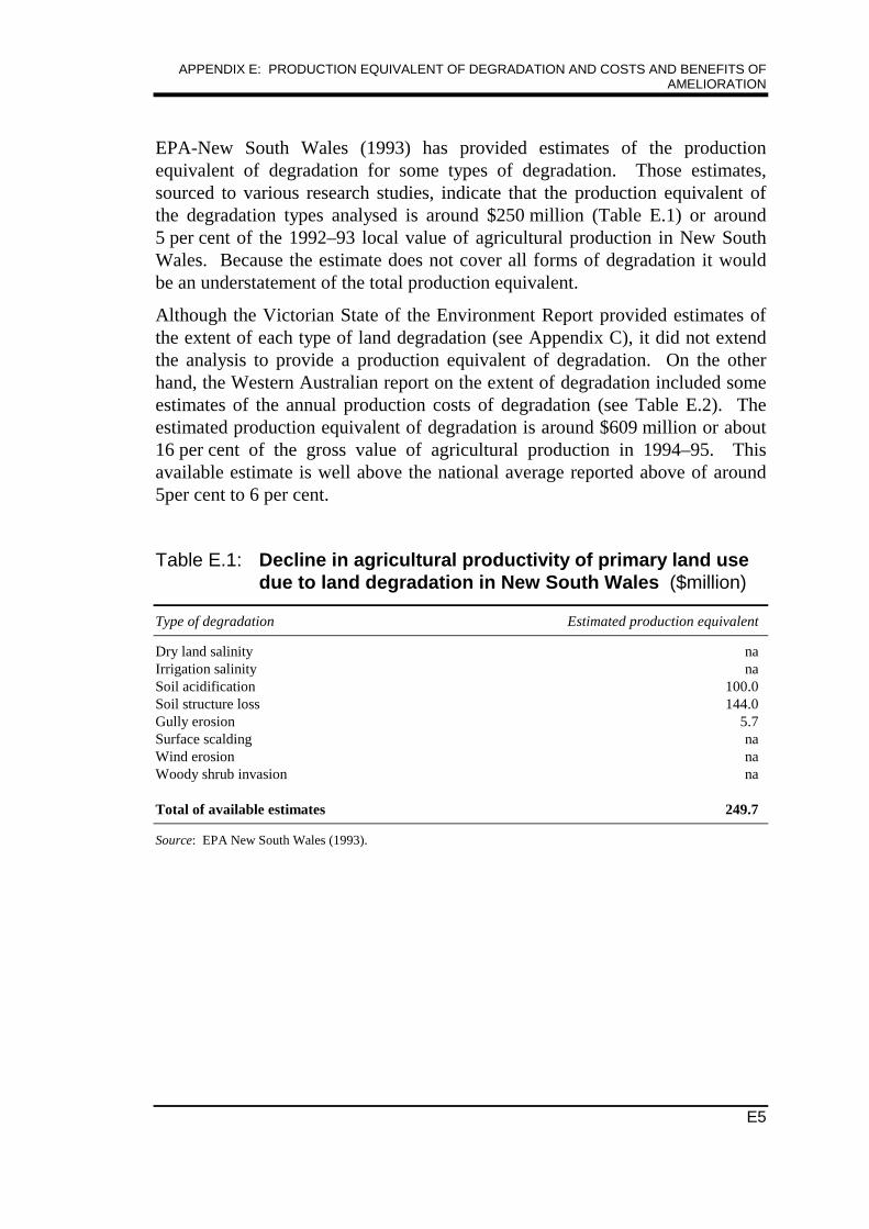
APPENDIX E: PRODUCTION EQUIVALENT OF DEGRADATION AND COSTS AND BENEFITS OFAMELIORATION
E5
EPA-New South Wales (1993) has provided estimates of the productionequivalent of degradation for some types of degradation. Those estimates,sourced to various research studies, indicate that the production equivalent ofthe degradation types analysed is around $250 million (Table E.1) or around5 per cent of the 1992–93 local value of agricultural production in New SouthWales. Because the estimate does not cover all forms of degradation it wouldbe an understatement of the total production equivalent.
Although the Victorian State of the Environment Report provided estimates ofthe extent of each type of land degradation (see Appendix C), it did not extendthe analysis to provide a production equivalent of degradation. On the otherhand, the Western Australian report on the extent of degradation included someestimates of the annual production costs of degradation (see Table E.2). Theestimated production equivalent of degradation is around $609 million or about16 per cent of the gross value of agricultural production in 1994–95. Thisavailable estimate is well above the national average reported above of around5per cent to 6 per cent.
Table E.1: Decline in agricultural productivity of primary land usedue to land degradation in New South Wales ($million)
Type of degradation Estimated production equivalent
Dry land salinity naIrrigation salinity naSoil acidification 100.0Soil structure loss 144.0Gully erosion 5.7Surface scalding naWind erosion naWoody shrub invasion na
Total of available estimates 249.7
Source: EPA New South Wales (1993).
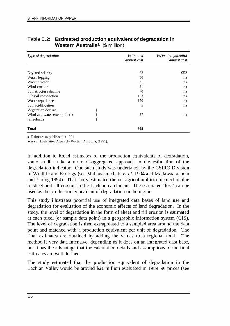
STAFF INFORMATION PAPER
E6
Table E.2: Estimated production equivalent of degradation inWestern Australiaa ($ million)
Type of degradation Estimatedannual cost
Estimated potentialannual cost
Dryland salinity 62 952Water logging 90 naWater erosion 21 naWind erosion 21 naSoil structure decline 70 naSubsoil compaction 153 naWater repellence 150 naSoil acidification 5 naVegetation declineWind and water erosion in therangelands
}}}
37 na
Total 609
a Estimates as published in 1991.Source: Legislative Assembly Western Australia, (1991).
In addition to broad estimates of the production equivalents of degradation,some studies take a more disaggregated approach to the estimation of thedegradation indicator. One such study was undertaken by the CSIRO Divisionof Wildlife and Ecology (see Mallawaarachchi et al. 1994 and Mallawaarachchiand Young 1994). That study estimated the net agricultural income decline dueto sheet and rill erosion in the Lachlan catchment. The estimated ‘loss’ can beused as the production equivalent of degradation in the region.
This study illustrates potential use of integrated data bases of land use anddegradation for evaluation of the economic effects of land degradation. In thestudy, the level of degradation in the form of sheet and rill erosion is estimatedat each pixel (or sample data point) in a geographic information system (GIS).The level of degradation is then extrapolated to a sampled area around the datapoint and matched with a production equivalent per unit of degradation. Thefinal estimates are obtained by adding the values to a regional total. Themethod is very data intensive, depending as it does on an integrated data base,but it has the advantage that the calculation details and assumptions of the finalestimates are well defined.
The study estimated that the production equivalent of degradation in theLachlan Valley would be around $21 million evaluated in 1989–90 prices (see
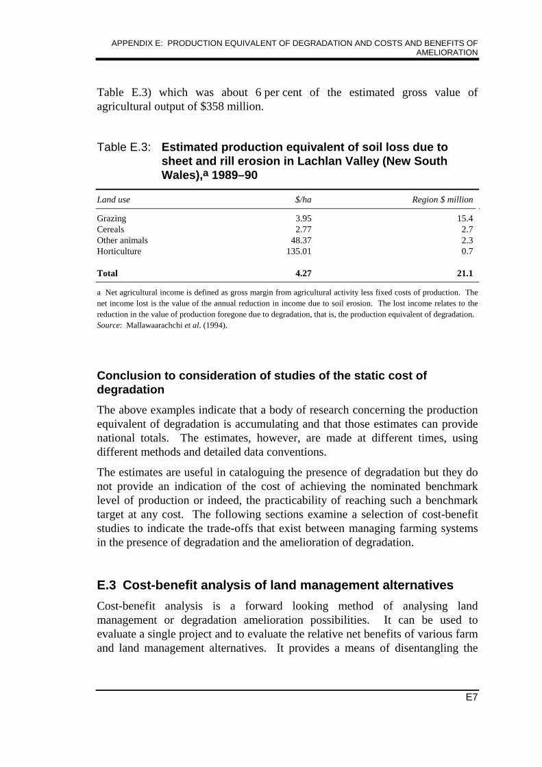
APPENDIX E: PRODUCTION EQUIVALENT OF DEGRADATION AND COSTS AND BENEFITS OFAMELIORATION
E7
Table E.3) which was about 6 per cent of the estimated gross value ofagricultural output of $358 million.
Table E.3: Estimated production equivalent of soil loss due tosheet and rill erosion in Lachlan Valley (New SouthWales),a 1989–90
Land use $/ha Region $ million
Grazing 3.95 15.4Cereals 2.77 2.7Other animals 48.37 2.3Horticulture 135.01 0.7
Total 4.27 21.1
a Net agricultural income is defined as gross margin from agricultural activity less fixed costs of production. Thenet income lost is the value of the annual reduction in income due to soil erosion. The lost income relates to thereduction in the value of production foregone due to degradation, that is, the production equivalent of degradation.Source: Mallawaarachchi et al. (1994).
Conclusion to consideration of studies of the static cost ofdegradation
The above examples indicate that a body of research concerning the productionequivalent of degradation is accumulating and that those estimates can providenational totals. The estimates, however, are made at different times, usingdifferent methods and detailed data conventions.
The estimates are useful in cataloguing the presence of degradation but they donot provide an indication of the cost of achieving the nominated benchmarklevel of production or indeed, the practicability of reaching such a benchmarktarget at any cost. The following sections examine a selection of cost-benefitstudies to indicate the trade-offs that exist between managing farming systemsin the presence of degradation and the amelioration of degradation.
E.3 Cost-benefit analysis of land management alternatives
Cost-benefit analysis is a forward looking method of analysing landmanagement or degradation amelioration possibilities. It can be used toevaluate a single project and to evaluate the relative net benefits of various farmand land management alternatives. It provides a means of disentangling the
STAFF INFORMATION PAPER
E8
relative merits of different projects. Cost-benefit analysis is concerned in oneform with commercial profitability and in another with the worth of a project tosociety, on the assumption that commercial profitability is not always a goodindicator of social worth. The first form of cost-benefit analysis is typicallyreferred to as financial analysis with the second as economic analysis.
Financial analysis emphasises market prices and the financial viability of aproject to its implementor (eg an individual farm). In financial analysis, anindividual enterprise would normally be concerned with maximising after taxincome in the context of current market prices, taxation arrangements andtariffs; and only limited objectives relating to the conduct of the individualproject, or program of closely related projects would be considered.
Economic analysis emphasises the opportunity cost of resources used and theeconomic viability of a project from the point of view of the community. Ineconomic analysis, governments would be more concerned to ensure thatprograms are contributing to community welfare. Such analyses wouldtherefore attempt to remove the effect of market distortions from prices and takeinto account externalities associated with land use as a social cost.
Both financial and economic analyses are concerned with the incremental outputand costs of a project and the evaluation of a stream of net benefits on the basisof their net present value.
The main differences between financial analysis and economic analysis concernthe way in which costs and benefits are defined, the prices used to value costsand benefits, and the selection of discount rates (see Box E.1). In contrast tocosts and benefits in financial analysis, economic costs and benefits are notnarrowly defined in terms of individual farmers cash flows, but rather aredefined in terms of the effect of the project on the community as a whole.
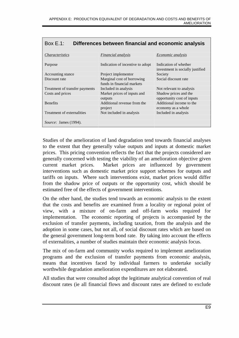
APPENDIX E: PRODUCTION EQUIVALENT OF DEGRADATION AND COSTS AND BENEFITS OFAMELIORATION
E9
Box E.1: Differences between financial and economic analysis
Characteristics Financial analysis Economic analysis
Purpose Indication of incentive to adopt Indication of whetherinvestment is socially justified
Accounting stance Project implementor SocietyDiscount rate Marginal cost of borrowing
funds in financial marketsSocial discount rate
Treatment of transfer payments Included in analysis Not relevant to analysisCosts and prices Market prices of inputs and
outputsShadow prices and theopportunity cost of inputs
Benefits Additional revenue from theproject
Additional income to theeconomy as a whole
Treatment of externalities Not included in analysis Included in analysis
Source: James (1994).
Studies of the amelioration of land degradation tend towards financial analysesto the extent that they generally value outputs and inputs at domestic marketprices. This pricing convention reflects the fact that the projects considered aregenerally concerned with testing the viability of an amelioration objective givencurrent market prices. Market prices are influenced by governmentinterventions such as domestic market price support schemes for outputs andtariffs on inputs. Where such interventions exist, market prices would differfrom the shadow price of outputs or the opportunity cost, which should beestimated free of the effects of government interventions.
On the other hand, the studies tend towards an economic analysis to the extentthat the costs and benefits are examined from a locality or regional point ofview, with a mixture of on-farm and off-farm works required forimplementation. The economic reporting of projects is accompanied by theexclusion of transfer payments, including taxation, from the analysis and theadoption in some cases, but not all, of social discount rates which are based onthe general government long-term bond rate. By taking into account the effectsof externalities, a number of studies maintain their economic analysis focus.
The mix of on-farm and community works required to implement ameliorationprograms and the exclusion of transfer payments from economic analysis,means that incentives faced by individual farmers to undertake sociallyworthwhile degradation amelioration expenditures are not elaborated.
All studies that were consulted adopt the legitimate analytical convention of realdiscount rates (ie all financial flows and discount rates are defined to exclude
STAFF INFORMATION PAPER
E10
the effects of price changes). While adjusting for inflation can be sufficient toaccount for the effects of price changes, if there are relative price changes (ieterms of trade for the sector) inflation adjustments alone would not be sufficientto obtain costs and benefits in ‘real’ prices. If the analyst has good reason tobelieve that the value of output will decline (or increase) over time compared tothe value of other goods and services, the change in relative values should beincorporated in the stream of real net benefits. In the studies consulted, thefarmers’ terms of trade is generally assumed to be constant. In fact, there hasbeen a long history of decline in the agricultural terms of trade (ABARE 1994).According to the principles of cost benefit analysis, an expected continuation ofthe declining agricultural terms of trade would lower the attractiveness offarming, including amelioration efforts, relative to other land uses.
Because the focus of the studies consulted is on degradation management andamelioration projects, other agricultural investment opportunities are not rankedfor consideration in the overall task of agricultural land management. If theimplementation of independent projects is not limited by any budget constraint,projects that yield a positive net present value should be adopted. However, inreality, individual projects may compete for the same land resource on a farm orwithin a region, or there may be budget constraints. Where such conflicts arisethe decision rules for project evaluation need to be extended (Perkins 1994).Projects that compete for the same land resource are mutually exclusive in thesense that both could not proceed simultaneously. For example, a project to usea block for irrigation farming would be mutually exclusive to an alternativeproject to use the same block for dry land farming. For such projects,community welfare (in economic analysis) would be maximised by selecting theproject with the highest net present value after account is taken of on-farm andoff-farm benefits and costs. The individual farmer would maximise farmincome by selecting the project with the highest net present value of on-farmbenefits.
Where there is a single period budget constraint, there will be an incentive toselect projects that yield the greatest net receipts per unit of investment in thatperiod. Such projects would not necessarily have the highest net present valuebut would recover the investment in the shortest possible period. Alternatively,the budget constraint may not be limited to a single period, but rather relate tothe longer term. Where there is a longer-term budget constraint, the targetinternal rate of return (or discount rate) should be raised to the point where theprojects adopted just exhaust the available supply of funds.
In reality, public and private budget constraints on agricultural investment willapply. In addition, once ranked according to the above criteria, amelioration
APPENDIX E: PRODUCTION EQUIVALENT OF DEGRADATION AND COSTS AND BENEFITS OFAMELIORATION
E11
projects may not always be the most advantageous for the farming sector or thecommunity, either in the longer or shorter term.
Costs and benefits of amelioration of irrigation salinity
Murray Basin
The Murray Basin is part of the Murray-Darling Basin in south-eastern Australiaand covers approximately one-seventh of the land area of Australia. The RiverMurray drains central and northern Victoria, parts of southern New South Walesand South Australia. The Darling and Murrumbidgee rivers flow into theMurray. The Darling drains the northern and western region of New SouthWales and southern Queensland; the Murrumbidgee drains central and southernNew South Wales.
Problems of salinity in the Murray are due to significant natural saline flowsinto the river and the fact that it forms the only outlet to the sea for salinegroundwater in the Basin. The River Murray salinity problem is intensified bygroundwater discharge due to rainfall, clearing of vegetation and irrigation.
As part of a program to introduce integrated (or total) catchment management inthe Murray-Darling Basin, a Working Group was established to prepare aSalinity and Drainage Strategy (MDBMC 1987). The supporting analysisincluded, amongst other things, a cost-benefit analysis of ameliorating riversalinity over the next 30 years. Public salt interception schemes werediscounted at a real rate of 5 per cent and private land management schemeswere discounted at the higher private real rate of 10 per cent.
In the analysis, river salinity was treated as a symptom of land degradation aswell as being the result of natural saline conditions in the Basin with both landdegradation and naturally occurring salinity imposing costs on the community.Using river salinity as a reference, the main focus of the study was on schemesthat would reduce river salinity. The benchmark for assessing costs and benefitsof amelioration was the expected production losses as waterlogging becamemore widespread and watertables rose under current management practices overthe next 30 years. Estimates of the production equivalent of degradation due towater logging and salinisation amounted to over 10 per cent of the value ofproduction in 1985–86 rising to around 16 per cent in 2015 (see Table E.4).
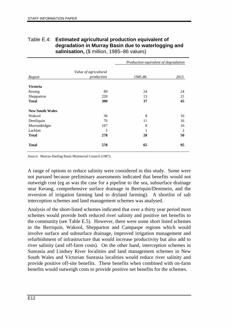
STAFF INFORMATION PAPER
E12
Table E.4: Estimated agricultural production equivalent ofdegradation in Murray Basin due to waterlogging andsalinisation, ($ million, 1985–86 values)
Production equivalent of degradation
RegionValue of agricultural
production 1985-86 2015
VictoriaKerang 80 24 24Shepparton 220 13 21Total 300 37 45
New South WalesWakool 36 8 16Deniliquin 70 11 16Murrumbidgee 167 8 16Lachlan 5 1 2Total 278 28 50
Total 578 65 95
Source: Murray-Darling Basin Ministerial Council (1987).
A range of options to reduce salinity were considered in this study. Some werenot pursued because preliminary assessments indicated that benefits would notoutweigh cost (eg as was the case for a pipeline to the sea, subsurface drainagenear Kerang, comprehensive surface drainage in Berriquin/Denimein, and thereversion of irrigation farming land to dryland farming). A shortlist of saltinterception schemes and land management schemes was analysed.
Analysis of the short-listed schemes indicated that over a thirty year period mostschemes would provide both reduced river salinity and positive net benefits tothe community (see Table E.5). However, there were some short listed schemesin the Berriquin, Wakool, Shepparton and Campaspe regions which wouldinvolve surface and subsurface drainage, improved irrigation management andrefurbishment of infrastructure that would increase productivity but also add toriver salinity (and off-farm costs). On the other hand, interception schemes inSunrasia and Lindsey River localities and land management schemes in NewSouth Wales and Victorian Sunrasia localities would reduce river salinity andprovide positive off-site benefits. These benefits when combined with on-farmbenefits would outweigh costs to provide positive net benefits for the schemes.
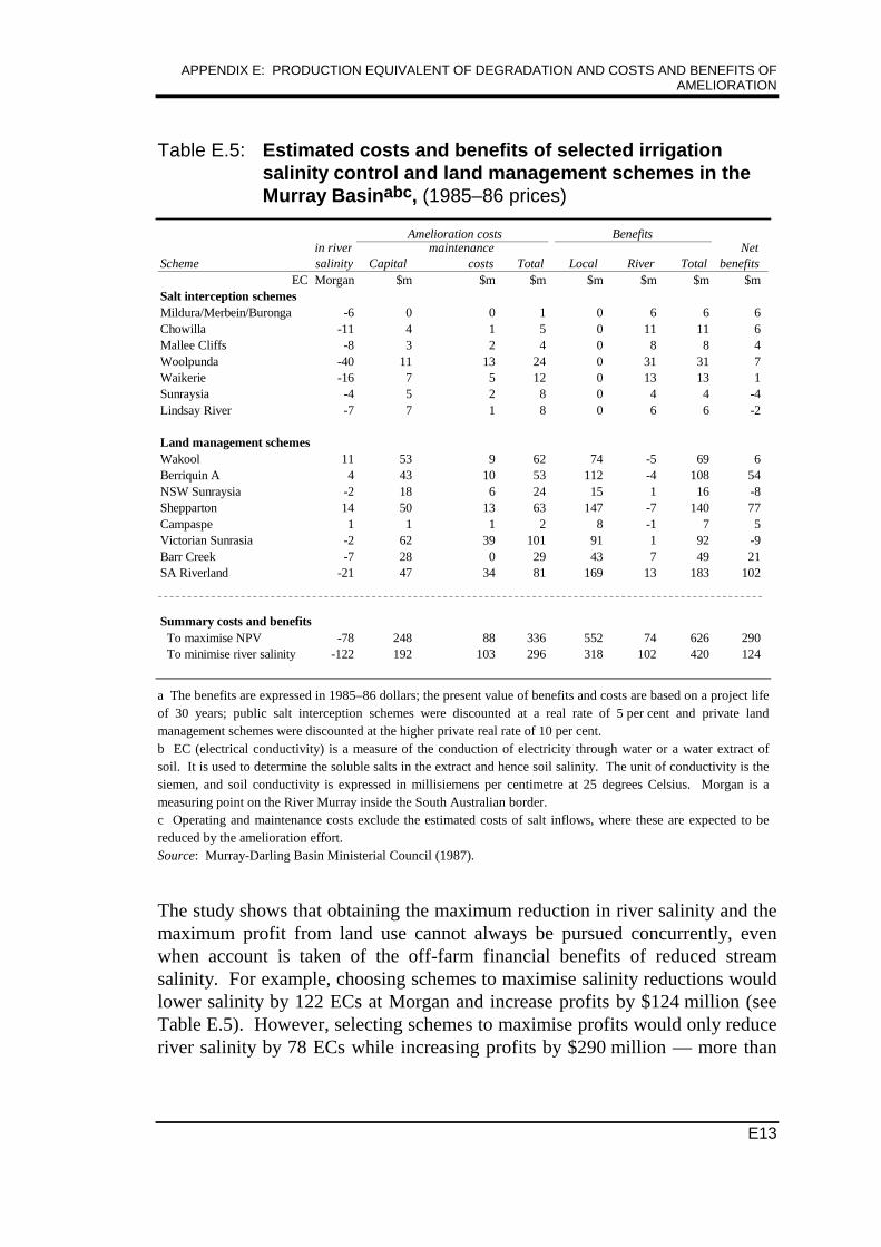
APPENDIX E: PRODUCTION EQUIVALENT OF DEGRADATION AND COSTS AND BENEFITS OFAMELIORATION
E13
Table E.5: Estimated costs and benefits of selected irrigationsalinity control and land management schemes in theMurray Basinabc, (1985–86 prices)
Amelioration costs Benefits
Schemein riversalinity Capital
maintenancecosts Total Local River Total
Netbenefits
EC Morgan $m $m $m $m $m $m $mSalt interception schemesMildura/Merbein/Buronga -6 0 0 1 0 6 6 6Chowilla -11 4 1 5 0 11 11 6Mallee Cliffs -8 3 2 4 0 8 8 4Woolpunda -40 11 13 24 0 31 31 7Waikerie -16 7 5 12 0 13 13 1Sunraysia -4 5 2 8 0 4 4 -4Lindsay River -7 7 1 8 0 6 6 -2
Land management schemesWakool 11 53 9 62 74 -5 69 6Berriquin A 4 43 10 53 112 -4 108 54NSW Sunraysia -2 18 6 24 15 1 16 -8Shepparton 14 50 13 63 147 -7 140 77Campaspe 1 1 1 2 8 -1 7 5Victorian Sunrasia -2 62 39 101 91 1 92 -9Barr Creek -7 28 0 29 43 7 49 21SA Riverland -21 47 34 81 169 13 183 102
Summary costs and benefits To maximise NPV -78 248 88 336 552 74 626 290 To minimise river salinity -122 192 103 296 318 102 420 124
a The benefits are expressed in 1985–86 dollars; the present value of benefits and costs are based on a project lifeof 30 years; public salt interception schemes were discounted at a real rate of 5 per cent and private landmanagement schemes were discounted at the higher private real rate of 10 per cent.b EC (electrical conductivity) is a measure of the conduction of electricity through water or a water extract ofsoil. It is used to determine the soluble salts in the extract and hence soil salinity. The unit of conductivity is thesiemen, and soil conductivity is expressed in millisiemens per centimetre at 25 degrees Celsius. Morgan is ameasuring point on the River Murray inside the South Australian border.c Operating and maintenance costs exclude the estimated costs of salt inflows, where these are expected to bereduced by the amelioration effort.Source: Murray-Darling Basin Ministerial Council (1987).
The study shows that obtaining the maximum reduction in river salinity and themaximum profit from land use cannot always be pursued concurrently, evenwhen account is taken of the off-farm financial benefits of reduced streamsalinity. For example, choosing schemes to maximise salinity reductions wouldlower salinity by 122 ECs at Morgan and increase profits by $124 million (seeTable E.5). However, selecting schemes to maximise profits would only reduceriver salinity by 78 ECs while increasing profits by $290 million — more than
STAFF INFORMATION PAPER
E14
double the best salinity reduction case. In the minimum salinity case,$102 million or 24 per cent of benefits could come from off-site effects whilefor the profit maximising case, $74 million or 10 per cent of benefits couldcome from off-site effects.
The estimated average level of salinity at Morgan (pre Menindee flowregulation) was 618 ECs (MDBMC 1987). The maximum salt reductionschemes would deliver a 20 per cent reduction on this total while the profitmaximisation schemes would lead to a 12 per cent reduction in salinity.
Costs and benefits of amelioration of dryland salinity
Dryland Campaspe Catchment, Victoria
The Campaspe Catchment is located in North Central Victoria and covers about454 800 hectares of which about two thirds is managed for agriculture. Thearea is bounded by the Great Dividing Range to the south and the CampaspeIrrigation District near Rochester to the north. The main land uses are grazingand cropping.
Problem salinity has led to increasing costs mainly through land salting andcontributions to the salt load in local rivers leading to the River Murray. Therelationship between farming systems, recharge and groundwater discharge wasexamined for the Campaspe Dryland Community Working Group on Salinity(Oram and Dumsday 1994).
Oram and Dumsday used a simulation model of groundwater recharge underalternative farm systems to evaluate the impact of land use on soil salting,salinisation of streams and rivers in the catchment, and the contribution of saltflows from the catchment to salinity levels in the River Murray. Theinformation was combined with a cost-benefit analysis to estimate the benefitsfrom the control of salinity, and the move from current agricultural land uses toalternative agricultural land uses. The analysis was undertaken for a 50-yearperiod. The discount rate adopted was a real rate of 4 per cent for off-farmbenefits and 8 per cent for on-farm returns. These rates were applied to theappropriate components of all projects.
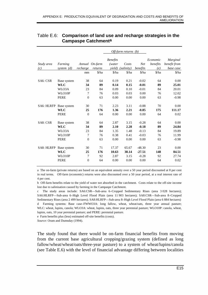
APPENDIX E: PRODUCTION EQUIVALENT OF DEGRADATION AND COSTS AND BENEFITS OFAMELIORATION
E15
Table E.6: Comparison of land use and recharge strategies in theCampaspe Catchmenta
Off-farm returns (b)
Study area (c)
Farming system (d)
Annualrecharge
On-farmreturns
Benefits(wateryield)
Costs(salinity)
Netbenefits
Economicbenefits
(e)
Marginalbenefit from
base casemm $/ha $/ha $/ha $/ha $/ha $/ha
SA6: CSR Base system 38 64 0.19 0.21 -0.02 64 0.00WLC 34 89 0.14 0.15 -0.01 89 25.01WLO3A 23 84 0.09 0.10 -0.01 84 20.01WLO10P 7 76 0.03 0.03 0.00 76 12.02PERE 0 63 0.00 0.00 0.00 63 -0.98
SA6: HLRFP Base system 30 71 2.23 3.11 -0.88 70 0.00WLC 25 176 1.36 2.21 -0.85 175 111.17PERE 0 64 0.00 0.00 0.00 64 0.02
SA8: CSR Base system 38 64 2.87 3.15 -0.28 64 0.00WLC 34 89 2.10 2.28 -0.18 89 24.84WLO3A 23 84 1.35 1.48 -0.13 84 19.89WLO10P 7 76 0.38 0.41 -0.03 76 11.99PERE 0 63 0.00 0.00 0.00 63 -0.98
SA8: HLRFP Base system 30 71 17.37 65.67 -48.30 23 0.00WLC 25 176 10.63 38.14 -27.51 148 84.51WLO10P 7 92 2.87 3.15 -0.28 92 27.74PERE 0 64 0.00 0.00 0.00 64 0.02
a The on-farm (private returns) are based on an equivalent annuity over a 50 year period discounted at 8 per centin real terms. Off-farm (economic) returns were also discounted over a 50 year period, at a real interest rate of4 per cent.b Off-farm benefits relate to the yield of water not absorbed in the catchment. Costs relate to the off-site incomelost due to salinisation caused by farming in the Campaspe Catchment.c The study areas include: SA6:CSR—Sub-area 6–Cropped Sedimentary Rises (area 3 028 hectares);SA6:HLRFP—Sub-area 6–High Level Flood Plain (area 11 903 hectares); SA8:CSR—Sub-area 8–CroppedSedimentary Rises (area 2 499 hectares); SA8:HLRFP—Sub-area 8–High Level Flood Plain (area 6 884 hectares)d Farming systems: Base case–FWWO3A: long fallow, wheat, wheat/oats, three year annual pasture;WLC: wheat, lupins, canola; WLO3A: wheat, lupins, oats, three year perennial pasture; WLO10P: canola, wheat,lupins, oats, 10 year perennial pasture; and PERE: perennial pasture.e Farm benefits plus (less) estimated off-site benefits (costs).Source: Oram and Dumsday (1994).
The study found that there would be on-farm financial benefits from movingfrom the current base agricultural cropping/grazing system (defined as longfallow/wheat/wheat/oats/three-year pasture) to a system of wheat/lupins/canola(see Table E.6) with the level of financial advantage differing between localities
STAFF INFORMATION PAPER
E16
within the region. However, the revised cropping rotation generally wouldprovide only marginal reductions in recharge compared to the base system. Theintroduction of perennial pasture would provide greater reductions ingroundwater recharge, but it was estimated that the additional economic gainsfrom off-site improvement in the form of reduced salinity would not offset thefinancial cost to farmers of reduced groundwater availability (with the effectthat the net off-site benefit is zero).
The study examined 12 farming systems including those reported in Table E.6.Alternatives were rejected if they increased recharge and hence could not berecommended as a salinity control strategy, or they decreased recharge but othermanagement systems achieved the same reduction at a lower cost. The high off-site costs of salinity in sub-area 8: HLRFP occur because of local ground watercharacteristics and proximity to the northern irrigation areas. The estimated off-site costs for this area are higher than the cropped water table rises which havethe highest recharge rates of the group examined.
Overall, the estimates indicate that the alternative yielding the most favourableagricultural industry outcome does not necessarily correspond to the case ofzero salt emissions. It also emphasises the importance of on-site benefitsrelative to off-site costs. As the analysis excludes agricultural practices thatincrease the level of dry land salinity, it has also possibly precluded options thatyield higher economic returns with higher levels of dryland salinity.
Neridup Catchment, Western Australia
The Neridup Catchment is located North East of Esperence, with an averagerainfall of about 500 mm (Campbell 1994). The total area of cleared arable landis 25 000 hectares containing approximately 25 farms. The land is mainly usedfor grazing (wool and beef) and cereal cropping (wheat, barley, oats and lupins).Induced salinity is estimated to cover 2 750 hectares (11 per cent) of the regionwith the biogeographical potential to reach 6 250 hectares (25 per cent) of theregion. Problem salinity is expanding at 87 hectares per year under currentmanagement, implying that the salinisation potential would be reached over40 years. In addition, farm productivity would be reduced through wind erosionand water logging as dryland salinity advances.
A cost-benefit analysis of amelioration possibilities in the region estimated thatthere would be benefits to farmers from the control of the spread of salinityachieved through increasing the area of trees and fodder shrubs and the buildingof salt drains (see Table E.7). The benefits would be realised through higherstocking rates and increases in crop yields. However, targeting a particular levelof salinity spread may not be profitable. For example, on available estimates, it
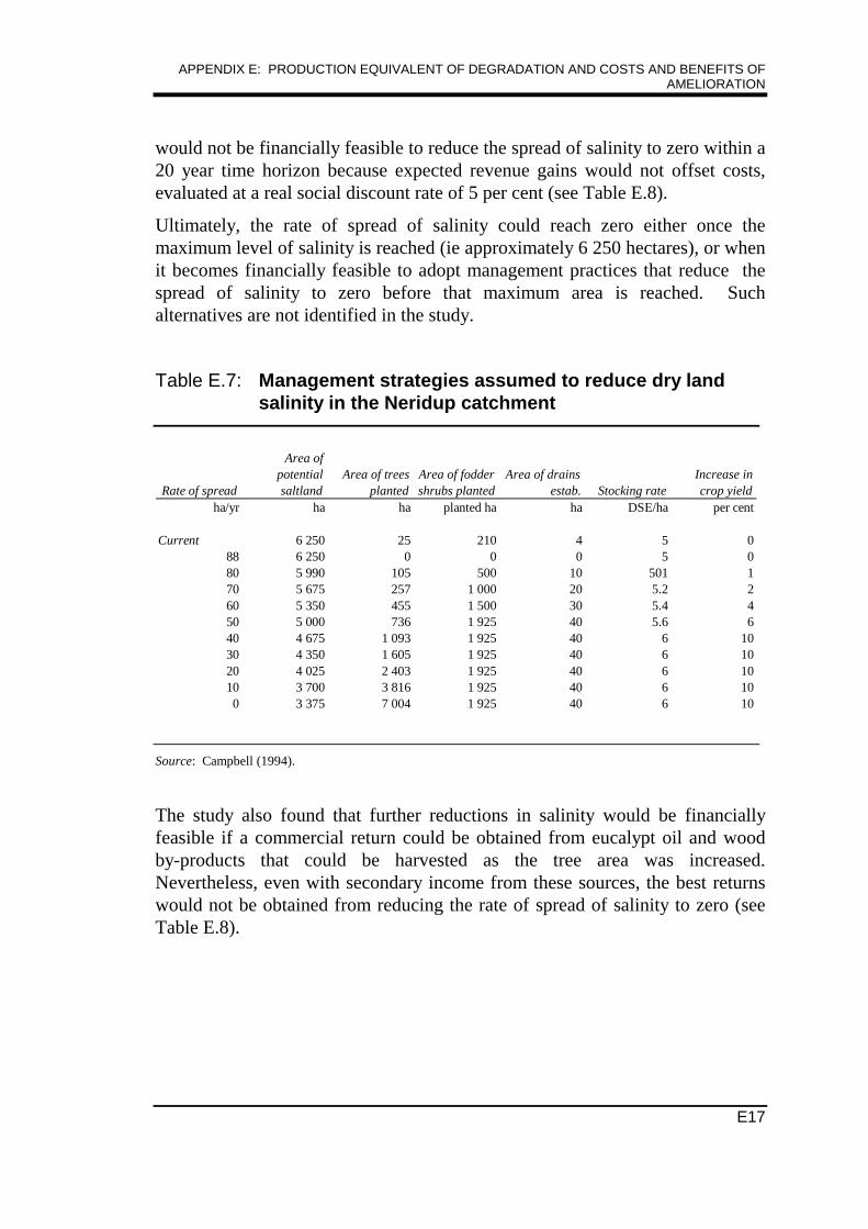
APPENDIX E: PRODUCTION EQUIVALENT OF DEGRADATION AND COSTS AND BENEFITS OFAMELIORATION
E17
would not be financially feasible to reduce the spread of salinity to zero within a20 year time horizon because expected revenue gains would not offset costs,evaluated at a real social discount rate of 5 per cent (see Table E.8).
Ultimately, the rate of spread of salinity could reach zero either once themaximum level of salinity is reached (ie approximately 6 250 hectares), or whenit becomes financially feasible to adopt management practices that reduce thespread of salinity to zero before that maximum area is reached. Suchalternatives are not identified in the study.
Table E.7: Management strategies assumed to reduce dry landsalinity in the Neridup catchment
Rate of spread
Area ofpotentialsaltland
Area of treesplanted
Area of foddershrubs planted
Area of drainsestab. Stocking rate
Increase incrop yield
ha/yr ha ha planted ha ha DSE/ha per cent
Current 6 250 25 210 4 5 088 6 250 0 0 0 5 080 5 990 105 500 10 501 170 5 675 257 1 000 20 5.2 260 5 350 455 1 500 30 5.4 450 5 000 736 1 925 40 5.6 640 4 675 1 093 1 925 40 6 1030 4 350 1 605 1 925 40 6 1020 4 025 2 403 1 925 40 6 1010 3 700 3 816 1 925 40 6 100 3 375 7 004 1 925 40 6 10
Source: Campbell (1994).
The study also found that further reductions in salinity would be financiallyfeasible if a commercial return could be obtained from eucalypt oil and woodby-products that could be harvested as the tree area was increased.Nevertheless, even with secondary income from these sources, the best returnswould not be obtained from reducing the rate of spread of salinity to zero (seeTable E.8).
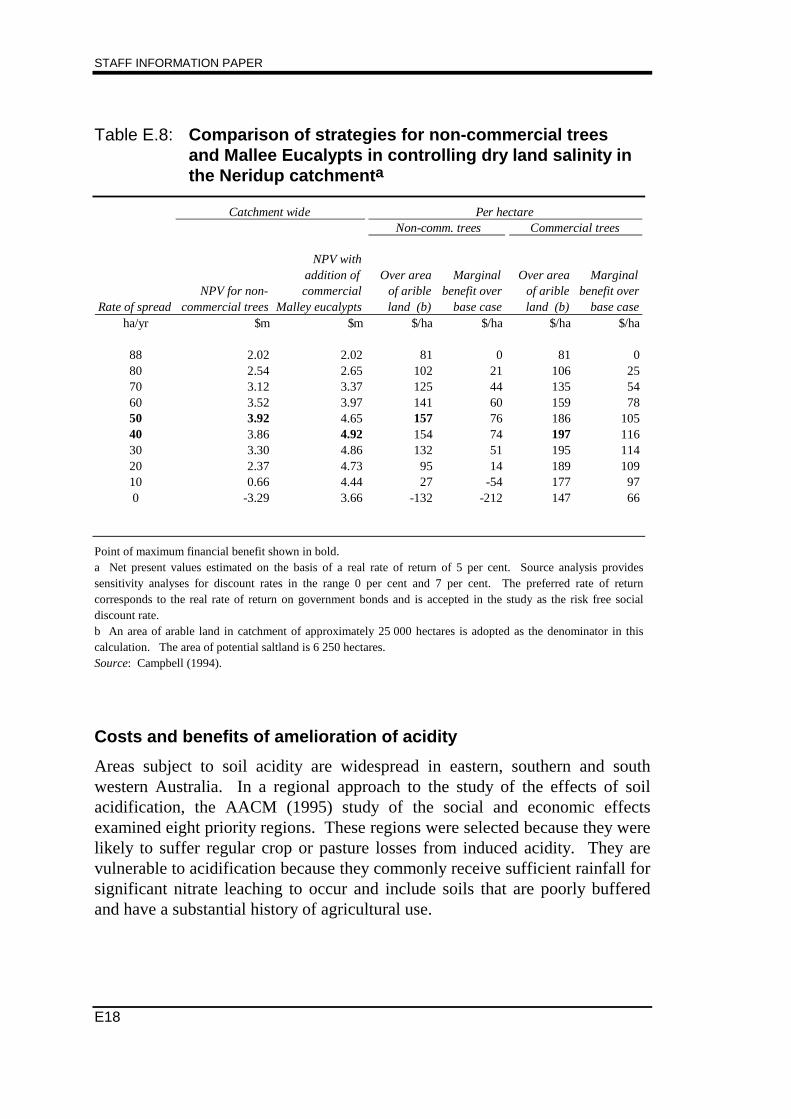
STAFF INFORMATION PAPER
E18
Table E.8: Comparison of strategies for non-commercial treesand Mallee Eucalypts in controlling dry land salinity inthe Neridup catchmenta
Catchment wide Per hectareNon-comm. trees Commercial trees
Rate of spreadNPV for non-
commercial trees
NPV withaddition ofcommercial
Malley eucalypts
Over areaof aribleland (b)
Marginalbenefit over
base case
Over areaof aribleland (b)
Marginalbenefit over
base caseha/yr $m $m $/ha $/ha $/ha $/ha
88 2.02 2.02 81 0 81 080 2.54 2.65 102 21 106 2570 3.12 3.37 125 44 135 5460 3.52 3.97 141 60 159 7850 3.92 4.65 157 76 186 10540 3.86 4.92 154 74 197 11630 3.30 4.86 132 51 195 11420 2.37 4.73 95 14 189 10910 0.66 4.44 27 -54 177 970 -3.29 3.66 -132 -212 147 66
Point of maximum financial benefit shown in bold.a Net present values estimated on the basis of a real rate of return of 5 per cent. Source analysis providessensitivity analyses for discount rates in the range 0 per cent and 7 per cent. The preferred rate of returncorresponds to the real rate of return on government bonds and is accepted in the study as the risk free socialdiscount rate.b An area of arable land in catchment of approximately 25 000 hectares is adopted as the denominator in thiscalculation. The area of potential saltland is 6 250 hectares.Source: Campbell (1994).
Costs and benefits of amelioration of acidity
Areas subject to soil acidity are widespread in eastern, southern and southwestern Australia. In a regional approach to the study of the effects of soilacidification, the AACM (1995) study of the social and economic effectsexamined eight priority regions. These regions were selected because they werelikely to suffer regular crop or pasture losses from induced acidity. They arevulnerable to acidification because they commonly receive sufficient rainfall forsignificant nitrate leaching to occur and include soils that are poorly bufferedand have a substantial history of agricultural use.
APPENDIX E: PRODUCTION EQUIVALENT OF DEGRADATION AND COSTS AND BENEFITS OFAMELIORATION
E19
One method of ameliorating induced soil acidity is through the application oflime. The balance between use and replenishment of soil alkalies can thereforebe illustrated by estimating lime applications required to balance excess acidsand replace alkalinity removed from the soil in farm production against actuallime use. Overall, it is estimated that the current level of lime applications inAustralian agriculture of about 0.5 million tonnes (1989–90) is about onequarter of the lime required to maintain prevailing acidity levels, withbenchmark maintenance applications comprising :
• 0.75 million tonnes per year to maintain the current pH in 7.4 millionhectares thought to be very acid or extremely acid in cropping areas; and
• 1.5 million tonnes per year to maintain the pH in 7.7 million hectares ofmildly acidic soils which are at risk from acidification (AACM 1995).
In addition, around 2.3 million tonnes of lime would be required to treat thesuspected 1.5 million hectares of extremely acid soil (pHCa<4.5) with anameliorative dressing of 1.5 tonnes per hectare.
Despite these physical accounting balances and the fact that lime applicationswould raise soil pH and increase production, a cost-benefit analysis of liming ina number of acid sensitive regions and farming systems shows that suchstrategies are not necessarily profitable (see Table E.9).
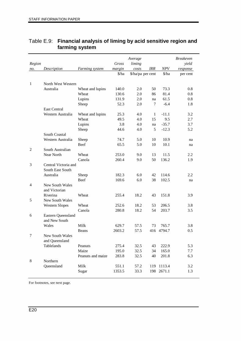
STAFF INFORMATION PAPER
E20
Table E.9: Financial analysis of liming by acid sensitive region andfarming system
Region no. Description Farming system
Gross margin
Average liming
costs IRR NPV
Breakeven yield
response$/ha $/ha/pa per cent $/ha per cent
1 North West Western Australia Wheat and lupins 140.0 2.0 50 73.3 0.8
Wheat 130.6 2.0 86 81.4 0.8Lupins 131.9 2.0 na 61.5 0.8Sheep 52.3 2.0 7 -6.4 1.8
East Central Western Australia Wheat and lupins 25.3 4.0 1 -11.1 3.2
Wheat 49.5 4.0 15 9.5 2.7Lupins 3.8 4.0 na -35.7 3.7Sheep 44.6 4.0 5 -12.3 5.2
South Coastal Western Australia Sheep 74.7 5.0 10 10.9 na
Beef 65.5 5.0 10 10.1 na2 South Australian
Near North Wheat 253.0 9.0 13 11.5 2.2Canola 260.4 9.0 50 136.2 1.9
3 Central Victoria and South East South Australia Sheep 182.3 6.0 42 114.6 2.2
Beef 169.6 6.0 38 102.5 na4 New South Wales
and Victorian Riverina Wheat 255.4 18.2 43 151.8 3.9
5 New South Wales Western Slopes Wheat 252.6 18.2 53 206.5 3.8
Canola 280.8 18.2 54 203.7 3.56 Eastern Queensland
and New South Wales Milk 629.7 57.5 73 765.7 3.8
Beans 2603.2 57.5 416 4794.7 0.57 New South Wales
and Queensland Tablelands Peanuts 275.4 32.5 43 222.9 5.3
Maize 195.0 32.5 34 165.0 7.7Peanuts and maize 283.8 32.5 40 201.8 6.3
8 Northern Queensland Milk 551.1 57.2 119 1113.4 3.2
Sugar 1353.5 33.3 198 2671.1 1.3
For footnotes, see next page.
APPENDIX E: PRODUCTION EQUIVALENT OF DEGRADATION AND COSTS AND BENEFITS OFAMELIORATION
E21
a The base case for the financial analysis of each farming system was the respective system without liming. Areal discount rate of 10 per cent was used and the analysis was conducted over a 15-year period to demonstratethe longer-term benefits of lime application.b Liming costs include the cost of the lime, transport of the lime to the farm site and spreading.c Gross margin per hectare in this analysis is defined as farm cash operating surplus being average yield perhectare less expenses on seed and seed treatment, chemicals, fuel and machinery, repairs and maintenance,labour, interest paid and insurance, and the costs of animal health, fodder, and stock purchases.d The internal rate of return is the discount rate that returns a net present value of zero.e The breakeven yield response to lime is the NPV increase in yield required to cover the NPV of the cost oflime and its application.Source: AACM (1995).
The study shows that the higher returns from liming tend to be associated withfarming systems with the higher gross margins per hectare (see Figure E.2). Notsurprisingly, the AACM study of farm enterprise practices found that limingwas a feature for those activities which are highly acidifying and for which highvalue farming systems were acid sensitive (eg dairying, horticulture, and canolaand lucerne crops). For other farming enterprises, the dominant strategy is touse liming selectively to raise soil pH levels once induced acidification isaffecting productivity or reducing farm capabilities, to grow high value crops.Strategies other than liming for dealing with acidifying soils include:
• dependence on acid tolerant species and cultivars (particularly in pastureenterprises);
• inputs of phosphorus (P), other nutrients and trace elements such asmolybdenum (Mo) to maintain the productivity of acidifying soils;
• use of dolomite rather than lime to avoid a manganese deficiency in dairycattle possibly caused by lime use;
• nitrogen management to reduce acidification rates and promote maximumplant use and minimum excess nitrate production; or
• do no additional work as there are better alternative farm or off-farminvestments.
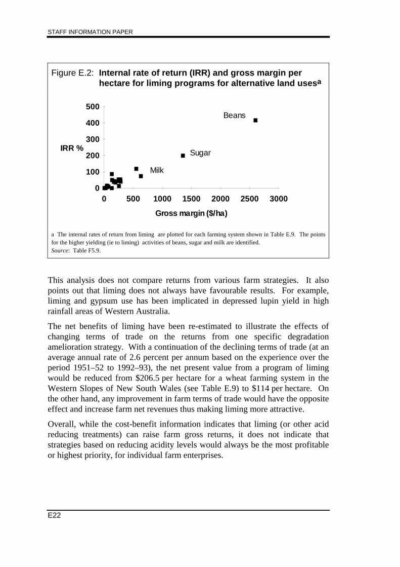
STAFF INFORMATION PAPER
E22
Figure E.2: Internal rate of return (IRR) and gross margin perhectare for liming programs for alternative land usesa
Gross margin ($/ha)
IR R %
0
100
200
300
400
500
0 500 1000 1500 2000 2500 3000
Beans
S ugar
Milk
a The internal rates of return from liming are plotted for each farming system shown in Table E.9. The pointsfor the higher yielding (ie to liming) activities of beans, sugar and milk are identified.Source: Table F5.9.
This analysis does not compare returns from various farm strategies. It alsopoints out that liming does not always have favourable results. For example,liming and gypsum use has been implicated in depressed lupin yield in highrainfall areas of Western Australia.
The net benefits of liming have been re-estimated to illustrate the effects ofchanging terms of trade on the returns from one specific degradationamelioration strategy. With a continuation of the declining terms of trade (at anaverage annual rate of 2.6 percent per annum based on the experience over theperiod 1951–52 to 1992–93), the net present value from a program of limingwould be reduced from $206.5 per hectare for a wheat farming system in theWestern Slopes of New South Wales (see Table E.9) to $114 per hectare. Onthe other hand, any improvement in farm terms of trade would have the oppositeeffect and increase farm net revenues thus making liming more attractive.
Overall, while the cost-benefit information indicates that liming (or other acidreducing treatments) can raise farm gross returns, it does not indicate thatstrategies based on reducing acidity levels would always be the most profitableor highest priority, for individual farm enterprises.
APPENDIX E: PRODUCTION EQUIVALENT OF DEGRADATION AND COSTS AND BENEFITS OFAMELIORATION
E23
E.4 Summing up
Taken alone, static measures of land degradation, such as those provided by theproduction equivalent of degradation, can be used to indicate the economiceffects of degradation. They can even be used to indicate a loss to theagricultural industry and the economy as a whole from degradation. However,such measures need to be interpreted with care as they ignore the income thathas been generated in the past through the use of the land and the trade offsfacing individual farmers and the community in the management of land.
Secondly, land degradation and its amelioration deals with only one aspect ofoverall land management decisions. Therefore, while recent cost-benefit studiesshow that net benefits can be obtained from degradation management andamelioration, they do not comment on how those projects might compare withother investment programs also affecting the land. The analyses show thatenvironmental objectives form one element in land management. They alsoshow that nominating environmental objectives, as a method of rankingprojects, would not necessarily provide the highest returns to the community interms of income. The selection of projects to achieve some environmentalbenefits would therefore need to depend on community judgements that gobeyond the information contained in cost-benefits analyses or the commercialimperatives facing individual farmers.

F1
APPENDIX FESTIMATES OF THE EFFECTS OF LANDDEGRADATION IN NEW SOUTH WALES
F.1 Introduction
In this appendix, an econometric model has been used to analyse the effects ofdegradation on agriculture in New South Wales. Currently, there is no otherstate-wide study analysing economic and land degradation data with which tocompare the Commission’s estimates. In the absence of a history of state-wideor national estimation of the effects of degradation on production and profits,the magnitude and even the sign of the estimates reported in this appendixshould be regarded as tentative. The modelling framework and results arepresented in order to encourage discussion and further analysis.1
The model uses cross-section data for 148 Statistical Local Areas (SLAs) inNew South Wales grouped into broad biogeographic regions (Appendix B).The data for each SLA cover indexes of production and costs for the 1992–93agricultural year. These indexes were estimated from 1991–92 and 1992–93source information drawn from ABS and ABARE series (see Annex F2). Landdegradation information was drawn from the 1987–1988 New South Wales SoilConservation Service state-wide survey of land degradation (see Appendix C).
The cross-sectional analysis captures differences in the responsiveness of SLAsto relative output price and input cost changes given the constraints on changeimposed by natural biogeographical endowments and prevailing levels of landdegradation. In this sense, even though the model is a snapshot of New SouthWales agriculture, it provides a medium- to longer-run perspective on theeffects of degradation.
Section F.2 reports the revenue and cost shares, price index and farm profitinformation underlying the econometric model estimation. Section F.3 providesan overview of the model. This section is supported by a more detailedstatement of the model and its data sources in Annexes F1 and F2. Section F.4provides the estimated responsiveness of agricultural outputs and inputs to
1 For those interested in re-estimating the model or undertaking further reviews of the data
and methodologies, the estimation data base and input files to the SHAZAM econometricpackage are available from the Commission on request.
STAFF INFORMATION PAPER
F2
relative price changes. These estimates are used to make a limited comparisonbetween results of the Commission’s model and other studies of Australian/New South Wales agriculture within a similar econometric framework. SectionF.5 draws land degradation and production information together to provide ananalysis of the snapshot effects of land degradation on farm outputs andprofitability in New South Wales. Section F.6 provides a summary of findings.
F.2 Agricultural output and input shares and price indexes
The agricultural output, input and price index data base, together withinformation on land degradation provide the basis of the Commission’s modelestimation. Details of the sources used to compute the modelling data base areprovided in Annex F.2. This section provides a state-wide summary of theinformation.
On the output side, production from New South Wales agriculture wassummarised by two commodity groups, namely, crops and crop products(henceforth referred to as crops) and animals and animal products (henceforthreferred to as animal products). The first group includes grains, fodder, oilseed, vegetable, and fruit products, while the second group includes livestock,wool, milk, eggs and honey products. Over the period studied, animal productscontributed more than half of the local value of production of New South Walesfarming industry (see Table F.1). This contribution rose fractionally from1991–92 to 1992–93 due to an increase in animal product prices relative to cropprices (see Table F.2).
On the input side, farm inputs were initially divided into four groups, namelyhired labour, fertiliser, water and other materials and services. Total returns tofarm management, capital and land (henceforth referred to as farm surplus orprofit) was then calculated as a residual by deducting the cost of purchasedinputs from the value of farm outputs. The items fertiliser and water use wereseparated in the analysis because of their association with intensive land use andtheir potential to increase the level of degradation. When combined theyaccount for less than 6 per cent of total costs (see Table F.1), with that sharefalling between 1991–92 and 1992–93 due to declining input volumes (seeTable F.3). The remaining intermediate input item — other materials andservices — includes farm expenses such as marketing costs, fuel and chemicalsand farm services (such as contractor, accounting and legal services). Despite asmall increase in average prices paid for items in this group (see Table F.2), itsshare in total costs declined over the two-year period due to a decline in inputvolumes (see Table F.3).
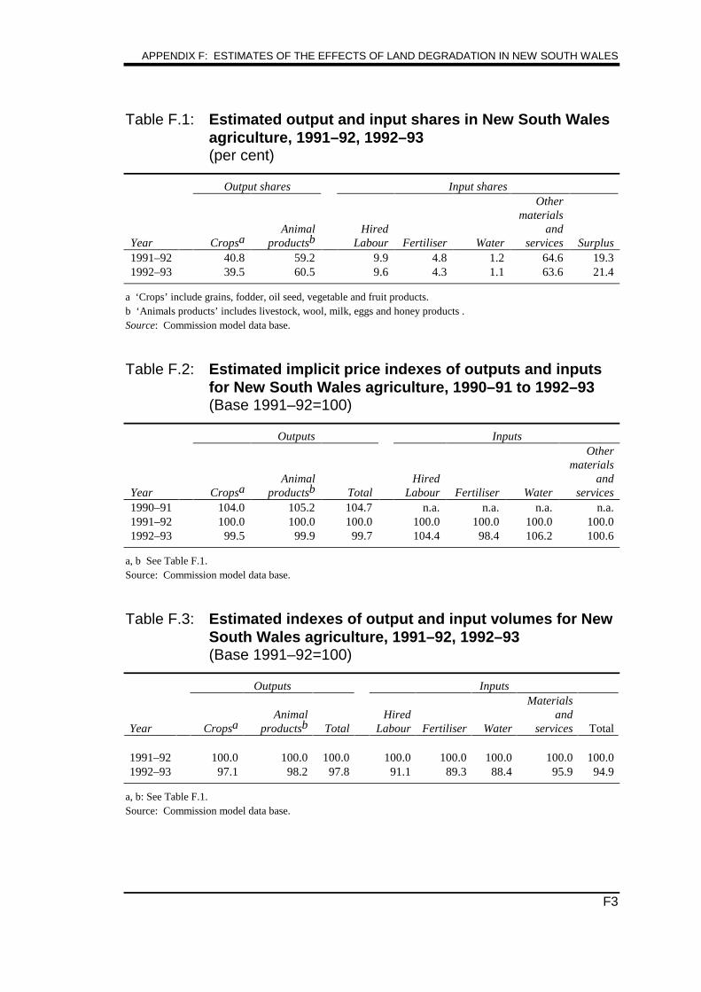
APPENDIX F: ESTIMATES OF THE EFFECTS OF LAND DEGRADATION IN NEW SOUTH WALES
F3
Table F.1: Estimated output and input shares in New South Walesagriculture, 1991–92, 1992–93(per cent)
Output shares Input shares
Year CropsaAnimal
productsbHired
Labour Fertiliser Water
Othermaterials
andservices Surplus
1991–92 40.8 59.2 9.9 4.8 1.2 64.6 19.31992–93 39.5 60.5 9.6 4.3 1.1 63.6 21.4
a ‘Crops’ include grains, fodder, oil seed, vegetable and fruit products.b ‘Animals products’ includes livestock, wool, milk, eggs and honey products .Source: Commission model data base.
Table F.2: Estimated implicit price indexes of outputs and inputsfor New South Wales agriculture, 1990–91 to 1992–93(Base 1991–92=100)
Outputs Inputs
Year CropsaAnimal
productsb TotalHired
Labour Fertiliser Water
Othermaterials
andservices
1990–91 104.0 105.2 104.7 n.a. n.a. n.a. n.a.1991–92 100.0 100.0 100.0 100.0 100.0 100.0 100.01992–93 99.5 99.9 99.7 104.4 98.4 106.2 100.6
a, b See Table F.1.Source: Commission model data base.
Table F.3: Estimated indexes of output and input volumes for NewSouth Wales agriculture, 1991–92, 1992–93(Base 1991–92=100)
Outputs Inputs
Year CropsaAnimal
productsb TotalHired
Labour Fertiliser Water
Materialsand
services Total
1991–92 100.0 100.0 100.0 100.0 100.0 100.0 100.0 100.01992–93 97.1 98.2 97.8 91.1 89.3 88.4 95.9 94.9
a, b: See Table F.1.Source: Commission model data base.
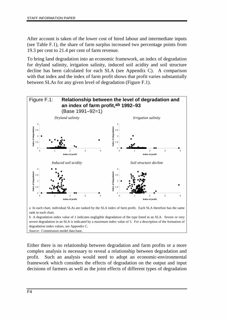
STAFF INFORMATION PAPER
F4
After account is taken of the lower cost of hired labour and intermediate inputs(see Table F.1), the share of farm surplus increased two percentage points from19.3 per cent to 21.4 per cent of farm revenue.
To bring land degradation into an economic framework, an index of degradationfor dryland salinity, irrigation salinity, induced soil acidity and soil structuredecline has been calculated for each SLA (see Appendix C). A comparisonwith that index and the index of farm profit shows that profit varies substantiallybetween SLAs for any given level of degradation (Figure F.1).
Figure F.1: Relationship between the level of degradation andan index of farm profit,ab 1992–93(Base 1991–92=1)
Dryland salinity Irrigation salinity
Index of profit
Ind
ex o
f d
egra
dat
ion
1
1.5
2
2.5
3
0 1 2 3 4
Index of profit
Ind
ex o
f d
egra
dat
ion
1
1.5
2
2.5
3
0 1 2 3 4
Induced soil acidity Soil structure decline
Index of profit
Ind
ex o
f d
egra
dat
ion
1
1.5
2
2.5
3
0 1 2 3 4
Index of profit
Ind
ex o
f d
egra
dat
ion
1
1.5
2
2.5
3
0 1 2 3 4
a In each chart, individual SLAs are ranked by the SLA index of farm profit. Each SLA therefore has the samerank in each chart.b A degradation index value of 1 indicates negligible degradation of the type listed in an SLA. Severe or verysevere degradation in an SLA is indicated by a maximum index value of 3. For a description of the formation ofdegradation index values, see Appendix C.Source: Commission model data base.
Either there is no relationship between degradation and farm profits or a morecomplex analysis is necessary to reveal a relationship between degradation andprofit. Such an analysis would need to adopt an economic-environmentalframework which considers the effects of degradation on the output and inputdecisions of farmers as well as the joint effects of different types of degradation
APPENDIX F: ESTIMATES OF THE EFFECTS OF LAND DEGRADATION IN NEW SOUTH WALES
F5
occurring in the same SLA and biogeographic region in which the SLA islocated.
An econometric model of New South Wales agriculture has been adopted inorder to investigate the relationship between degradation and profits for NewSouth Wales.
F.3 Model outline
The econometric model is based on the profit-maximising behaviour ofindividual farmers. The modelling approach is developed from establishedprocedures for variable profit function analysis. Annex F.1 sets out a detailedspecification of the model adopted.
The model maintains the hypothesis that farmers choose both variable input andoutput mixes to maximise current profits given a set of input and output prices,land degradation and other fixed factors. The assumption that farmers are pricetakers is appropriate because the farm sector produces standard commoditiesthat are typically traded on world markets and is characterised by manyproducers each supplying a small part of total domestic output.
Structure of the model
The model evaluates the responses of farmers to changing conditions on thebasis of a cross section of New South Wales agricultural industry datadisaggregated into 148 SLAs. The model incorporates two commodity outputcategories:
• crops and other plant products (crops); and
• animals and animal products (animal products);
while variable inputs are divided into four categories:
• hired labour;
• fertiliser;
• water (including water rates); and
• other materials and services (the numeraire for the model).
The fixed factors of production are:
• the area of agricultural land holdings; and
• farmer and farm manager labour;
with the effects of degradation being analysed with reference to:
STAFF INFORMATION PAPER
F6
• dryland salinity;
• irrigation salinity;
• soil structure decline; and
• induced soil acidity.
These types of degradation are a subset of the list of degradation types discussedin Appendix A. Of the other types, sheet and rill and wind erosion wereexcluded from the econometric analysis because the relevant degradationindexes are highly correlated with the degradation index for soil structuredecline which is included.
In order to account for biogeographical differences affecting the nature of farmactivity between SLAs, the following six New South Wales regional variableswere included in the model:
• North Coast;
• Central and South coast;
• Tablelands;
• Central areas;
• Central-west areas; and
• Western areas.
In addition, the effects of irrigation farming were captured through an irrigationregional variable. The biogeographical regional groupings are defined in termsof component SLAs as set out in Appendix B. Irrigation areas are all thoseSLAs for which the area of agricultural land irrigated exceeds 10 per cent ofagricultural land holdings in that SLA.
The econometrically estimated model was found to have a high degree ofexplanatory power. Some details about the statistical significance of the model,its estimates and the test results as well as some theoretical properties of themodel are reported in Box F.1. While, with some qualification, the tests provideencouragement for the use of the model, ultimately, it must be evaluated on thebasis of the economic meaningfulness of its estimates and insights that it canadd to the discussion of land degradation and Australian agricultural industry.
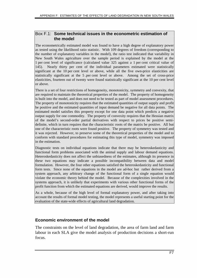
APPENDIX F: ESTIMATES OF THE EFFECTS OF LAND DEGRADATION IN NEW SOUTH WALES
F7
Box F.1: Some technical issues in the econometric estimation ofthe model
The econometrically estimated model was found to have a high degree of explanatory poweras tested using the likelihood ratio statistic. With 109 degrees of freedom (corresponding tothe number of explanatory variables in the model), the ratio test indicated that variability inNew South Wales agriculture over the sample period is explained by the model at the1 per cent level of significance (calculated value 325 against a 1 per cent critical value of145). Nearly thirty per cent of the individual parameters estimated were statisticallysignificant at the 10 per cent level or above, while all the five own-price elasticities arestatistically significant at the 5 .per cent level or above. Among the set of cross-priceelasticities, fourteen out of twenty were found statistically significant at the 10 per cent levelor above.
There is a set of four restrictions of homogeneity, monotonicity, symmetry and convexity, thatare required to maintain the theoretical properties of the model. The property of homogeneityis built into the model, and does not need to be tested as part of model assessment procedures.The property of monotonicity requires that the estimated quantities of output supply and profitbe positive and the estimated quantities of input demand be negative for all data points. Theestimated model satisfies this property except for one data point which predicts a negativeoutput supply for one commodity. The property of convexity requires that the Hessian matrixof the model’s second-order partial derivatives with respect to prices be positive semi-definite, which in turn requires that the characteristic roots of the matrix be positive. All butone of the characteristic roots were found positive. The property of symmetry was tested andit was rejected. However, to preserve some of the theoretical properties of the model and toconform with standard procedures for estimating this type of model, symmetry was imposedin the estimation.
Diagnostic tests on individual equations indicate that there may be heteroskedasticity andfunctional form problems associated with the animal supply and labour demand equations.Heteroskedasticity does not affect the unbiasedness of the estimates, although its presence inthese two equations may indicate a possible incompatibility between data and modelformulation. However, the four other equations satisfied the heteroskedasticity and functionalform tests. Since none of the equations in the model are ad-hoc but rather derived from asystem approach, any arbitrary change of the functional form of a single equation wouldviolate the economic theory behind the model. Because of the complexities involved in thesystems approach, it is unlikely that experiments with various other functional forms of theprofit function from which the estimated equations are derived, would improve the results.
As a whole, because of the high level of formal explanatory power, and after taking intoaccount the results of formal model testing, the model represents a useful starting point for theevaluation of the state-wide effects of agricultural land degradation.
Economic environment of the model
The constraints on the level of land degradation, the area of farm land and farmlabour in each SLA give the model analysis of production decisions a short-runfocus.
STAFF INFORMATION PAPER
F8
In addition, there is substantial variability in the level of degradation betweenSLAs (see Figure F.1). This variability has enabled the assumption of fixeddegradation to be relaxed to give a medium- to longer-run perspective on theeffects of land degradation. The cross-section modelling approach supports theanalysis of this added perspective by evaluating the variability of the level ofland degradation, production and profits between SLAs. The medium- tolonger-run property of the data is used in this study to analyse the effects of achange in degradation for New South Wales agriculture.
Profit maximising (or loss minimising) farmers would be expected to trade offhigher degradation and profit in the current period, against conservation of theland in the current period for production and profit in the future. The outcomeof the trade off made by the farmer is embodied in the measure of farm profit,defined in the model as gross revenue less variable input costs of production.Therefore, the measure of profit reflects both current income and theopportunity cost of future resource use. In this sense, decisions made in thecurrent period involve a consideration of possible future income flows and theoutcome of decisions is captured in the model.
F.4 Responsiveness of agricultural outputs and inputs torelative price changes
The responsiveness of agricultural inputs and outputs to relative price changes ismeasured by own and cross-price elasticities (see Table F.4). The elasticitiesare computed at the sample mean, and represent the state-average for NewSouth Wales. The model estimates elasticities for five items: crops, animalproducts, labour, fertiliser, and water. The elasticities of the numeraire variableother materials and services are not directly estimated, but derived residuallyfrom other parameters (see Annex F.1).
The economic environment relevant for the estimation of price elasticities in themodel has a short-run focus. That is the elasticities are estimated with the areaof agricultural land, farm management labour and land degradation assumedfixed.
Own price effects
The own-price elasticities appear on the diagonal of Table F.4 and report theestimated percentage change in the volume of output (input) for a one percentchange in the price of that output (input) with all other output and input pricesheld constant. For example, a 1 per cent increase in the price of crops would
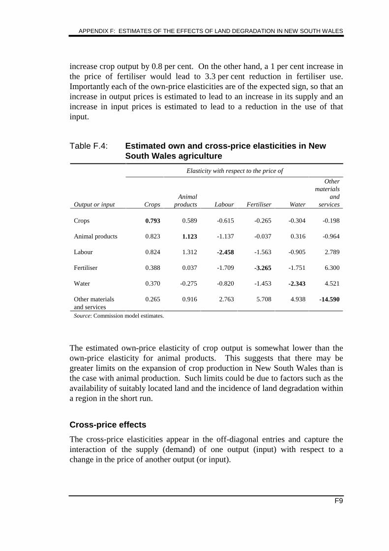
APPENDIX F: ESTIMATES OF THE EFFECTS OF LAND DEGRADATION IN NEW SOUTH WALES
F9
increase crop output by 0.8 per cent. On the other hand, a 1 per cent increase inthe price of fertiliser would lead to 3.3 per cent reduction in fertiliser use.Importantly each of the own-price elasticities are of the expected sign, so that anincrease in output prices is estimated to lead to an increase in its supply and anincrease in input prices is estimated to lead to a reduction in the use of thatinput.
Table F.4: Estimated own and cross-price elasticities in NewSouth Wales agriculture
Elasticity with respect to the price of
Output or input CropsAnimal
products Labour Fertiliser Water
Othermaterials
andservices
Crops 0.793 0.589 -0.615 -0.265 -0.304 -0.198
Animal products 0.823 1.123 -1.137 -0.037 0.316 -0.964
Labour 0.824 1.312 -2.458 -1.563 -0.905 2.789
Fertiliser 0.388 0.037 -1.709 -3.265 -1.751 6.300
Water 0.370 -0.275 -0.820 -1.453 -2.343 4.521
Other materialsand services
0.265 0.916 2.763 5.708 4.938 -14.590
Source: Commission model estimates.
The estimated own-price elasticity of crop output is somewhat lower than theown-price elasticity for animal products. This suggests that there may begreater limits on the expansion of crop production in New South Wales than isthe case with animal production. Such limits could be due to factors such as theavailability of suitably located land and the incidence of land degradation withina region in the short run.
Cross-price effects
The cross-price elasticities appear in the off-diagonal entries and capture theinteraction of the supply (demand) of one output (input) with respect to achange in the price of another output (or input).
STAFF INFORMATION PAPER
F10
On the output side, the analysis finds a complementary relationship betweenanimal products and crops. Thus, a one per cent increase in animal productprices is estimated to lead to an increase in New South Wales animal productoutput of 1.12 per cent and a complementary increase in crop output of0.59 per cent. There are a number of possible explanations for this finding.
In the first instance, animal and crop production are intrinsically complementaryin agriculture due to rotation systems of farming. In addition, thecomplementarity between crops and animal products can be associated withinput-output relationships that exist between these two products. Inspection ofAustralian input-output tables indicates that about 10 per cent of cropproduction goes as an input to the animal product industries either directly ashay and fodder or indirectly through stock feed products (ABS Cat. No. 5209.0).As the expected price of animal products rises and farmers respond by increasedproduction, crops production also needs to expand to meet the increased feeddemand of the animal sector. The extent to which national average linksportrayed in Australian input-output tables are accurate descriptions of regionalrelationships will depend on the agricultural industry structure of the region.The current analysis of New South Wales, as a whole, suggests that inter-industry flows evident at the national level prevail at the state level. Asubregion study may not find the same inter-industry links.
On the input side, the analysis also finds substitution and complementaryrelationships exist among inputs used in the New South Wales agriculturesector. For example, fertiliser and labour appear to be complementary to oneanother as indicated by a negative cross-price elasticity value of -1.71. Thisindicates that with a 1 per cent decrease in the price of labour fertiliser demandwould increase by 1.71 per cent, as labour demand also increases. On the otherhand, other materials and services is found to be a substitute for labour, fertiliserand water. This relationship is indicated by positive signs for the cross-priceelasticities appearing in the other materials and service row and column ofTable F.4. For example, a 1 per cent decrease in the price of labour is estimatedto reduce the demand for other materials and services by 2.8 per cent, as labourdemand increases.
Comparison with other studies
A number of other econometric studies of agriculture in Australia have beenundertaken using similar methodologies. While these studies are not strictlycomparable to this current study due to scope or timing differences, the modelsprovide useful benchmarks against which to consider the results of this study.
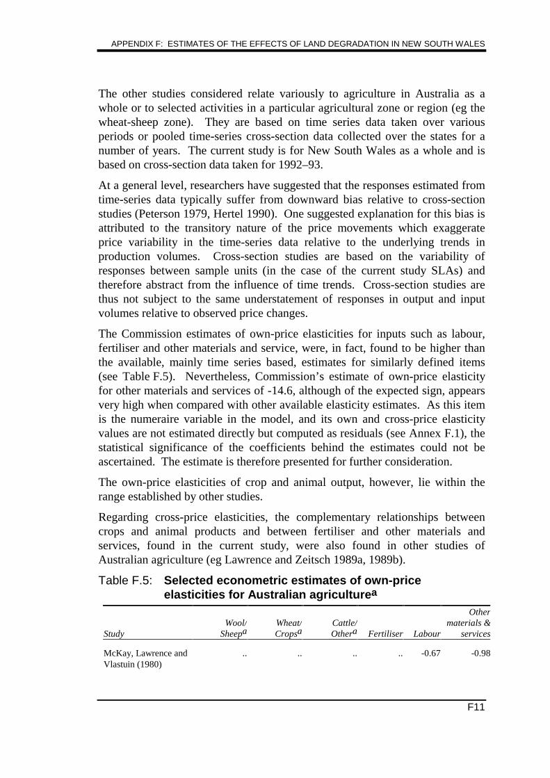
APPENDIX F: ESTIMATES OF THE EFFECTS OF LAND DEGRADATION IN NEW SOUTH WALES
F11
The other studies considered relate variously to agriculture in Australia as awhole or to selected activities in a particular agricultural zone or region (eg thewheat-sheep zone). They are based on time series data taken over variousperiods or pooled time-series cross-section data collected over the states for anumber of years. The current study is for New South Wales as a whole and isbased on cross-section data taken for 1992–93.
At a general level, researchers have suggested that the responses estimated fromtime-series data typically suffer from downward bias relative to cross-sectionstudies (Peterson 1979, Hertel 1990). One suggested explanation for this bias isattributed to the transitory nature of the price movements which exaggerateprice variability in the time-series data relative to the underlying trends inproduction volumes. Cross-section studies are based on the variability ofresponses between sample units (in the case of the current study SLAs) andtherefore abstract from the influence of time trends. Cross-section studies arethus not subject to the same understatement of responses in output and inputvolumes relative to observed price changes.
The Commission estimates of own-price elasticities for inputs such as labour,fertiliser and other materials and service, were, in fact, found to be higher thanthe available, mainly time series based, estimates for similarly defined items(see Table F.5). Nevertheless, Commission’s estimate of own-price elasticityfor other materials and services of -14.6, although of the expected sign, appearsvery high when compared with other available elasticity estimates. As this itemis the numeraire variable in the model, and its own and cross-price elasticityvalues are not estimated directly but computed as residuals (see Annex F.1), thestatistical significance of the coefficients behind the estimates could not beascertained. The estimate is therefore presented for further consideration.
The own-price elasticities of crop and animal output, however, lie within therange established by other studies.
Regarding cross-price elasticities, the complementary relationships betweencrops and animal products and between fertiliser and other materials andservices, found in the current study, were also found in other studies ofAustralian agriculture (eg Lawrence and Zeitsch 1989a, 1989b).
Table F.5: Selected econometric estimates of own-priceelasticities for Australian agriculturea
StudyWool/
SheepaWheat/Cropsa
Cattle/Othera Fertiliser Labour
Othermaterials &
services
McKay, Lawrence andVlastuin (1980)
.. .. .. .. -0.67 -0.98

STAFF INFORMATION PAPER
F12
Wicks and Dillon(1978)
0.25 1.10 0.69 .. .. ..
Vincent, Dixon andPowell (1980)b
0.25 .. 0.48 .. .. ..
Adams (1987) 0.46 .. 0.70 .. .. ..
McKay, Lawrence andVlastuin (1983)
0.72 0.50 0.12 .. -0.47 -0.10
Dewbre, Shaw andCorra (1985)
0.39 0.92 0.34 .. .. ..
Wall and Fisher (1987)c
Regions in NSW only
0.00 to 0.68 0.60 to 0.63 0.16 to 0.24 .. .. ..
Regions in other states
0.00 to 1.89 0.87 to 4.79 0.01 to 1.25 .. .. ..
Lawrence and Zeitsch(1989a)
.. 0.19 .. -1.26 -0.78 -0.33
Lawrence and Zeitsch(1989b)
.. .. .. .. -0.68 -0.53
IC (1995)d 1.23 0.80 .. -3.26 -2.45 -14.59
a Items from source studies are selected to coincide as closely as possible with the items listed in the tablecolumn headings.b Covers the wheat/sheep zone only.c Covers the sheep industry only.d New South Wales agriculture.Sources: As listed in the table.
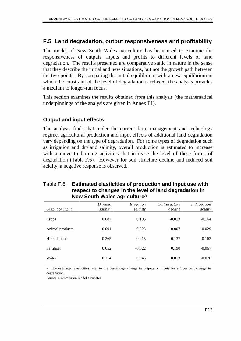
APPENDIX F: ESTIMATES OF THE EFFECTS OF LAND DEGRADATION IN NEW SOUTH WALES
F13
F.5 Land degradation, output responsiveness and profitability
The model of New South Wales agriculture has been used to examine theresponsiveness of outputs, inputs and profits to different levels of landdegradation. The results presented are comparative static in nature in the sensethat they describe the initial and new situations, but not the growth path betweenthe two points. By comparing the initial equilibrium with a new equilibrium inwhich the constraint of the level of degradation is relaxed, the analysis providesa medium to longer-run focus.
This section examines the results obtained from this analysis (the mathematicalunderpinnings of the analysis are given in Annex F1).
Output and input effects
The analysis finds that under the current farm management and technologyregime, agricultural production and input effects of additional land degradationvary depending on the type of degradation. For some types of degradation suchas irrigation and dryland salinity, overall production is estimated to increasewith a move to farming activities that increase the level of these forms ofdegradation (Table F.6). However for soil structure decline and induced soilacidity, a negative response is observed.
Table F.6: Estimated elasticities of production and input use withrespect to changes in the level of land degradation inNew South Wales agriculturea
Output or inputDrylandsalinity
Irrigationsalinity
Soil structuredecline
Induced soilacidity
Crops 0.087 0.103 -0.013 -0.164
Animal products 0.091 0.225 -0.007 -0.029
Hired labour 0.265 0.215 0.137 -0.162
Fertiliser 0.052 -0.022 0.190 -0.067
Water 0.114 0.045 0.013 -0.076
a The estimated elasticities refer to the percentage change in outputs or inputs for a 1 per cent change indegradation.Source: Commission model estimates.
STAFF INFORMATION PAPER
F14
One possible reason for the different effects of additional degradation issuggested by the different nature of dryland and irrigation salinity compared toinduced acidity and soil structure decline. In the case of dryland and irrigationsalinity, the nature of degradation is such that salinity is visible only at somelocalised spots rather than in the entire area (Box F.2). Because of the localisednature of visible severe degradation, a farmer could gain more from the increasein productivity in the cleared or irrigated land than productivity lost from thoseisolated points which develop problem salinity.
On the other hand, induced soil acidity and soil structure decline tends tocharacterise whole farming areas. In this situation, losses in productivity alsotend to be widespread affecting whole farming areas rather than individualpoints on an otherwise productive farm landscape. Thus the gains from farmingactivities which initiated these forms of degradation, are outweighed by thelosses resulting from reduced productivity.
Box F.2: Assessment of degradationDryland and irrigation salinity were assessed within a 100 ha circle centred on a sample point.With evidence of these forms of land degradation found within the circle, the sample pointwas coded as having that form of degradation. The highest severity value observed wasrecorded.
The severity of induced soil acidity and soil structure decline was assigned with respect to afour hectare quadrant around each sample point. The most severe severity class observed wasrecorded.
In the Soil Conservation Service-NSW analysis of its survey data, total areas affected byinduced soil acidity and soil structure decline were estimated by assuming that thedegradation noted for the sample point was representative of the surrounding area, andaggregating the area estimates across sample points using GIS techniques. However, fordryland and irrigation salinity, such aggregate area measures of degradation were not madebecause land degradation at a specific location does not represent the severity of degradationin the area surrounding the survey point.
The essential difference between the two groups of degradation is that the estimates of theseverity of dryland and irrigation salinity should not be viewed as representative of a localityor region while estimates of the severity of induced soil acidity and soil structure decline canbe viewed in that way.
The forms of land degradation and the estimates of the indexes of degradation severity arediscussed in Appendices A and C.
The model estimates also suggest that changing degradation would lead to asubstitution between farm inputs as outputs change. For example, theexpansion of activities associated with dryland and irrigation salinity appears
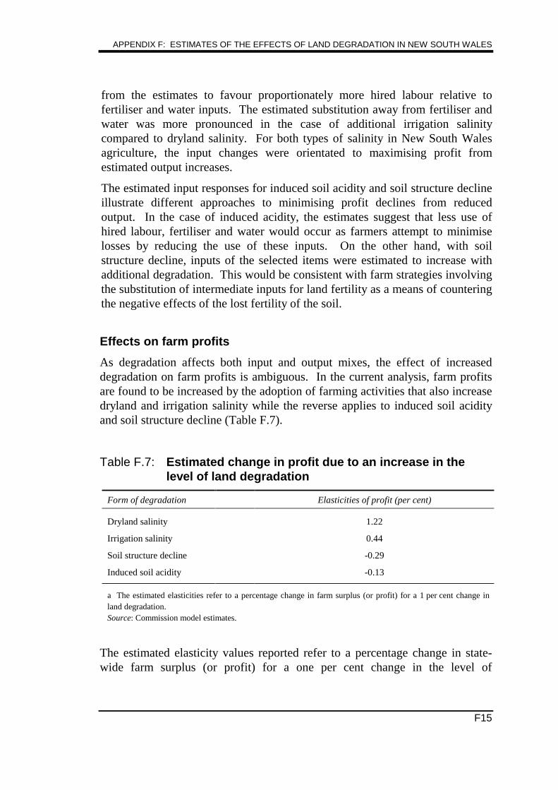
APPENDIX F: ESTIMATES OF THE EFFECTS OF LAND DEGRADATION IN NEW SOUTH WALES
F15
from the estimates to favour proportionately more hired labour relative tofertiliser and water inputs. The estimated substitution away from fertiliser andwater was more pronounced in the case of additional irrigation salinitycompared to dryland salinity. For both types of salinity in New South Walesagriculture, the input changes were orientated to maximising profit fromestimated output increases.
The estimated input responses for induced soil acidity and soil structure declineillustrate different approaches to minimising profit declines from reducedoutput. In the case of induced acidity, the estimates suggest that less use ofhired labour, fertiliser and water would occur as farmers attempt to minimiselosses by reducing the use of these inputs. On the other hand, with soilstructure decline, inputs of the selected items were estimated to increase withadditional degradation. This would be consistent with farm strategies involvingthe substitution of intermediate inputs for land fertility as a means of counteringthe negative effects of the lost fertility of the soil.
Effects on farm profits
As degradation affects both input and output mixes, the effect of increaseddegradation on farm profits is ambiguous. In the current analysis, farm profitsare found to be increased by the adoption of farming activities that also increasedryland and irrigation salinity while the reverse applies to induced soil acidityand soil structure decline (Table F.7).
Table F.7: Estimated change in profit due to an increase in thelevel of land degradation
Form of degradation Elasticities of profit (per cent)
Dryland salinity 1.22
Irrigation salinity 0.44
Soil structure decline -0.29
Induced soil acidity -0.13
a The estimated elasticities refer to a percentage change in farm surplus (or profit) for a 1 per cent change inland degradation.Source: Commission model estimates.
The estimated elasticity values reported refer to a percentage change in state-wide farm surplus (or profit) for a one per cent change in the level of
STAFF INFORMATION PAPER
F16
degradation. In 1992–93, the state-average farm surplus was estimated, fromthe Commission data base, to be $19 per hectare, with substantial regionalvariations around the average. Applying these elasticities to this state-wideaverage suggests that activities that have accompanying higher levels of salinitydegradation would raise the per hectare farm profit by $0.24 for dryland and$0.08 for irrigation salinity. The changes represent 1 per cent and 0.4 per cent,respectively, of state farm surplus. On the other hand, degradation associatedwith soil structure decline and induced soil acidity would lower average farmprofit by $0.06 and $0.03 per hectare, respectively, which represent0.03 per cent and 0.02 per cent, respectively, of state average surplus.
The above financial measures of the state-wide financial effects of degradationare very small when compared to the average profit per hectare. Given that landdegradation is a slow and gradual process, it could take a number of yearsbefore the cumulative negative effects of degradation become of sufficientimportance to enter into the farmer’s land management decision makingprocess.
Dynamic considerations
Because the analysis is based on a snapshot of New South Wales agriculture,estimates represent the likely effects of once and for all, marginal changes inland degradation. Thus, the model estimates do not infer the cumulative effectsof successive increases in degradation that would occur in the continuum ofland use. For example, the extension of farming activities that involve drylandand irrigation salinity could improve New South Wales farm output andprofitability as indicated by the model estimates even at the expense of somemore degradation. Progressively more and more land would be sacrificed todegradation, under prevailing technologies. Ultimately, the cumulative effect ofdryland and irrigation salinity could become negative. This possibility isillustrated in the model estimates of the negative effects of additional inducedsoil acidity and soil structure decline. They illustrate that at some pointdegradation can become so severe or so widespread that further increases reduceproduction and profit.
These analyses are concerned with the effects of degradation and thesubstitution between activities, given current technologies. They do not takeinto account the dynamic effects of technological change and other sources ofproductivity improvement. To be effective, technological changes wouldinvolve a shift to new farming activities that raise the productivity of the land.Such productivity changes could, in principle, be associated with higher orlower levels of degradation. A change that could involve more degradation
APPENDIX F: ESTIMATES OF THE EFFECTS OF LAND DEGRADATION IN NEW SOUTH WALES
F17
could be one that discounts the importance of the immediate condition of theland (eg., poultry farming, piggeries and cattle feedlots). Alternatively, thetechnological change could favour reductions in degradation to improve cropand pasture growth (eg introduction of minimum tillage techniques and/or saltand acid resistant plant species).
F.7 Summing up
An integrated profit function model has been used to analyse production, inputsand land degradation in New South Wales agriculture. The estimated priceelasticities capturing the link between output, inputs and price changes werefound to be of the expected sign. In addition, a substantial proportion of theparameter estimates were also statistically significant according to conventionaltests of significance. The estimates obtained were found to be around a range ofvalues suggested by other studies of Australian agriculture. If anything thecurrent analysis suggests that the input mix for agriculture may be somewhatmore flexible to relative price changes than previously estimated.
On the basis of this general assessment of the model, it was extended to providesome insights into degradation issues in a state-wide framework.
The general findings of the study indicate that at the current level ofdevelopment of the agricultural industry there are positive incentives for farmerswho are operating with evident salinity not to move away from those farmingsystems. However, for farmers who are operating with severely acid soil ordeteriorated structure in soil, the incentives would favour a shift to alternative,more profitable, farming activities. Similarly, in the case of salinity, there areincentives for other farmers to move towards those farming activities thatcoexist with higher levels of degradation. For the other two forms ofdegradation the incentives would appear to discourage a move to activities thatencourage additional induced acidity or soil structure decline.
The model results indicate that land management decisions, as they are appliedto degradation, influence farm production and profits. Depending on farmtechnologies, allowing some additional on-farm degradation may increaseprofits, or it may lead to reduced returns.
STAFF INFORMATION PAPER
F18
Annex F1: Econometric model of agriculture and the effectsof land degradation
Basic theoretical model
Given a set of product and input prices and a number of fixed factors of production such asfamily labour, area of agricultural land holdings, land characteristics, capital stock, weather,etc., farmers make decisions about output and input-mix. Assuming that they exhibit profitmaximising behaviour and that the markets where they operate are competitive, the farmerschoose their output and input mix in such a way that their expected variable profit, defined astotal revenue net of variable factor costs, is maximised. Thus, a farmer’s problem is tomaximise
Π = −PY RX subject to Y f X Z= ( ; ) (1)
where Π is profit, Y and X are vectors of outputs and variable inputs with P and R being
the respective vectors of prices, and Z is a vector of factors that remain fixed in the short-
run.
The first-order conditions of the problem yield optimal levels of outputs Y(P,R;Z) and ofinputs X(P,R;Z). Substituting these expressions for Y and X into (1) yields the indirect profitfunction Π° , which has the same arguments as Y and X,
Π Π∗ ∗= ( , ; )P R Z (2)
By applying Hotelling’s lemma, differentiating (2) with respect to the prices gives a set ofoutput supply and negative of input demand equations. Thus,
∂ ∂Π∗ =( , ; ) / ( , ; )P R Z P Y P R Zi i i=1,...,g (3)
and
∂ ∂Π∗ = −( , ; ) / ( , ; )P R Z R X P R Zj j j=g+1,...,n (4)
Equation (3) and (4) form the basic model representing farmers’ choice of output and input-mix in any one year when they face a given level of fixed factors of production and landdegradation.
Model specification and functional form
A wide range of functional forms is available to model production decisions involved inequations (2) to (4). The most commonly used are Cobb-Douglas or CES. While a Cobb-Douglas function restricts partial elasticities of substitution between all products to be equalto one, the CES form restricts them to be equal, but not necessarily to one. Among the moreflexible functional forms, those commonly used include: generalised Leontief, symmetricgeneralised McFadden, normalised quadratic, and transcendental logarithmic. These flexiblefunctional forms are nonlinear in the variables and they are termed flexible because they aresecond order, or Taylor series, approximations to any underlying actual production functions,
APPENDIX F: ESTIMATES OF THE EFFECTS OF LAND DEGRADATION IN NEW SOUTH WALES
F19
and they do not impose as many restrictions on the production technology as functional formssuch as Cobb-Douglas, CES or CRESH/CRETH.
These flexible functional forms have been developed for a variety of applications of appliedproduction theory, and there is not one particular function that can be expected to suit allpurposes. However, one common limiting factor present in most of these models in the pasthas been their failure to satisfy some curvature condition such as global convexity. Theunderlying economic theory behind deriving production technology from profit function isapplied duality.2 Global convexity of the profit function (that is, decreasing returns to scalein production) is a necessary condition for the duality to hold between profit and productionfunctions. If the condition of convexity does not hold for a model, which is more often thecase, it can be imposed by following one of the methods suggested by Wiley, Schmidt andBramble (1973), Lau (1978) and Jorgensen and Fraumeni (1981). However, Diewert andWales (1987) have shown that when convexity is imposed on a translog function, it collapsesto a Cobb-Douglas form and loses its flexibility. In fact, among the set of flexible functionalforms, the normalised quadratic function developed by Lau (1976) and the symmetricgeneralised McFadden function, developed by Diewert and Wales (1987) are the onlyfunctional forms on which global convexity can be imposed while retaining their flexibility.The normalised quadratic profit function also has the advantage of being self-dual, that is, theproduction function underlying a normalised quadratic profit function is also a quadraticfunction. This property is also shared by some other functional forms, such as Cobb-Douglasor CES, but they imply more rigid production structure.
Examples of studies using a normalised quadratic profit function to estimate the input demandand output supply elasticities are Shumway, Saez and Gottret (1988), Moschini (1988),Coxhead (1988), Maligaya and White (1989), Nehring (1991), Salma (1992), and Polson andShumway (1992). An example of the application of normalised quadratic functional form forAustralian agriculture is Wall and Fisher (1987, 1990) for its sheep industry study. TheSymmetric Generalised MacFadden function, a function similar to normalised quadratic, wasapplied by Lawrence (1990) and Lawrence and Zeitsch (1989a, 1989b) to study Australianagriculture.
The normalised quadratic functional form is adopted in this study to estimate the profit, inputdemand and output supply functions in New South Wales agriculture. The empirical modeluses information on agricultural outputs, commodity inputs, farmers and farm managers, landand land degradation. The variable profit function in (2) in normalised quadratic functionalform in this multi-output multi-input case is given by:
2 In essence duality theory states that under certain regularity conditions, the profit function
and the production function contain the same information about production technology. Adual approach, which uses a profit function rather than a production function, providesmore flexibility and econometrically it is a rigorous approach to the derivation of estimatesof technology parameters.
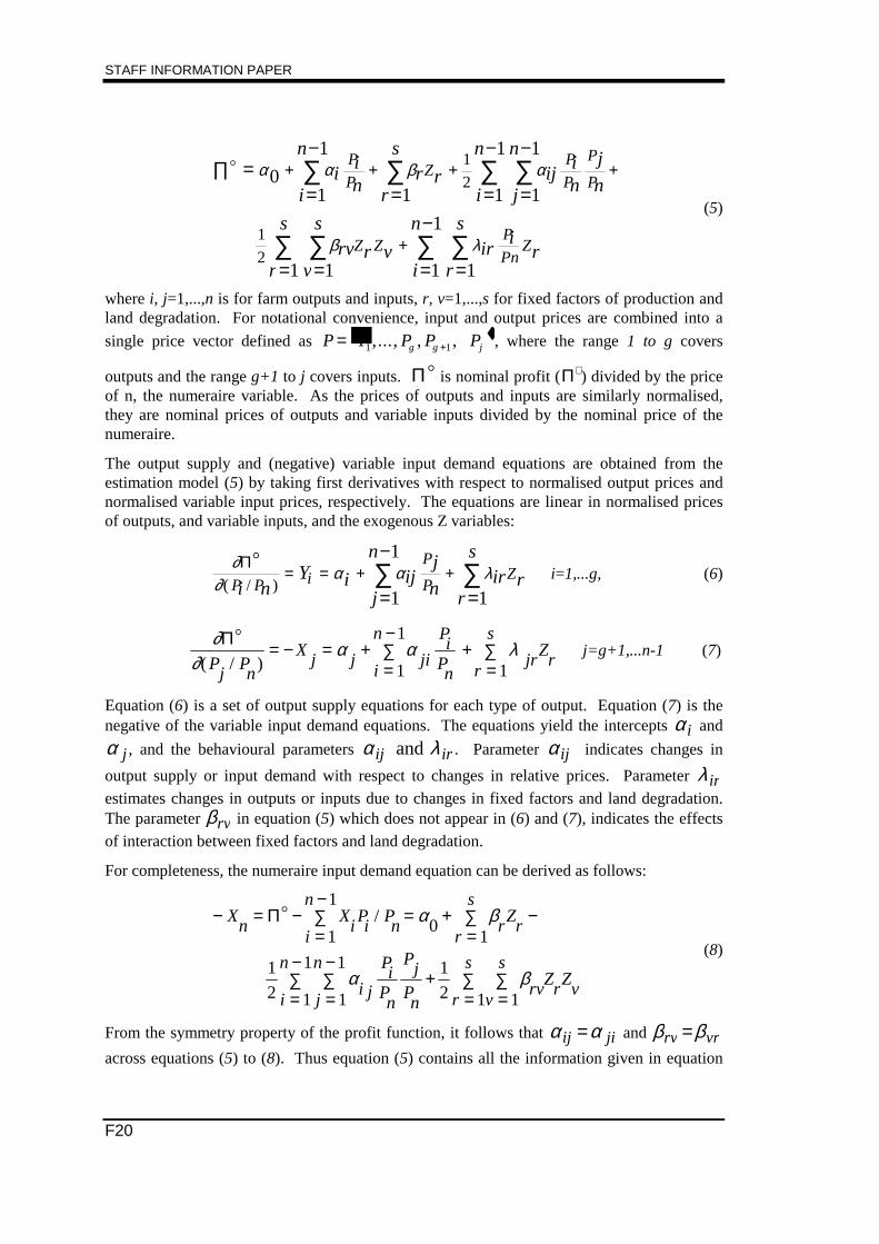
STAFF INFORMATION PAPER
F20
∏ ==
−
= =
−
=
−
= = =
−
=
+ + + +
+
∑ ∑ ∑ ∑
∑ ∑ ∑ ∑
� α α β α
β λ
01
1
1 1
1
1
1
1 1 1
1
1
1
2
1
2
ii
nin
rr
s
ri
nij
j
nin
j
n
r
srv
v
s
r vi
nir
r
si
r
P
PZ
P
P
P
P
Z ZP
PnZ
(5)
where i, j=1,...,n is for farm outputs and inputs, r, v=1,...,s for fixed factors of production andland degradation. For notational convenience, input and output prices are combined into a
single price vector defined as P P P P Pg g j= +1 1,..., , ,� �, where the range 1 to g covers
outputs and the range g+1 to j covers inputs. Π� is nominal profit (Π∗ ) divided by the priceof n, the numeraire variable. As the prices of outputs and inputs are similarly normalised,they are nominal prices of outputs and variable inputs divided by the nominal price of thenumeraire.
The output supply and (negative) variable input demand equations are obtained from theestimation model (5) by taking first derivatives with respect to normalised output prices andnormalised variable input prices, respectively. The equations are linear in normalised pricesof outputs, and variable inputs, and the exogenous Z variables:
∂∂
α α λΠ�
( / )P P iP
PZ
i nY i ij
j
n j
nir
r
s
r= = + +=
−
=∑ ∑
1
1
1 i=1,...g, (6)
∂∂
α α λΠ�
( / )Pj
Pn
Xj j ji
i
n Pi
Pn
jrr
sZ
r= − = +
=
−∑ +
=∑
1
1
1 j=g+1,...n-1 (7)
Equation (6) is a set of output supply equations for each type of output. Equation (7) is thenegative of the variable input demand equations. The equations yield the intercepts α i and
α j , and the behavioural parameters α λij irand . Parameter α ij indicates changes in
output supply or input demand with respect to changes in relative prices. Parameter λ irestimates changes in outputs or inputs due to changes in fixed factors and land degradation.The parameter βrv in equation (5) which does not appear in (6) and (7), indicates the effectsof interaction between fixed factors and land degradation.
For completeness, the numeraire input demand equation can be derived as follows:
− = −=
−∑ = +
=∑ −
=
−∑
=
−∑ +
=∑
=∑
Xn
XiPi
i
nPn r
r
sZ
r
i
n
i jj
n Pi
Pn
Pj
Pn r
s
rvv
sZ
rZ
v
Π�
1
1
01
1
2 1
1
1
1 1
2 1 1
/ α β
α β(8)
From the symmetry property of the profit function, it follows that α αij ji= and β βrv vr=across equations (5) to (8). Thus equation (5) contains all the information given in equation
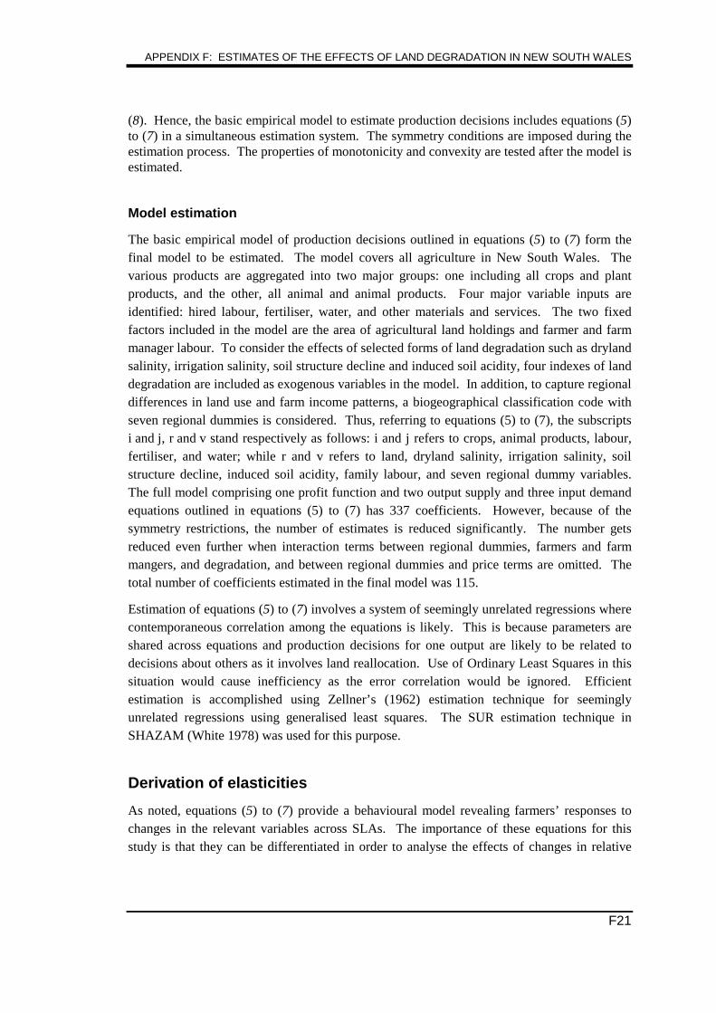
APPENDIX F: ESTIMATES OF THE EFFECTS OF LAND DEGRADATION IN NEW SOUTH WALES
F21
(8). Hence, the basic empirical model to estimate production decisions includes equations (5)to (7) in a simultaneous estimation system. The symmetry conditions are imposed during theestimation process. The properties of monotonicity and convexity are tested after the model isestimated.
Model estimation
The basic empirical model of production decisions outlined in equations (5) to (7) form thefinal model to be estimated. The model covers all agriculture in New South Wales. Thevarious products are aggregated into two major groups: one including all crops and plantproducts, and the other, all animal and animal products. Four major variable inputs areidentified: hired labour, fertiliser, water, and other materials and services. The two fixedfactors included in the model are the area of agricultural land holdings and farmer and farmmanager labour. To consider the effects of selected forms of land degradation such as drylandsalinity, irrigation salinity, soil structure decline and induced soil acidity, four indexes of landdegradation are included as exogenous variables in the model. In addition, to capture regionaldifferences in land use and farm income patterns, a biogeographical classification code withseven regional dummies is considered. Thus, referring to equations (5) to (7), the subscriptsi and j, r and v stand respectively as follows: i and j refers to crops, animal products, labour,fertiliser, and water; while r and v refers to land, dryland salinity, irrigation salinity, soilstructure decline, induced soil acidity, family labour, and seven regional dummy variables.The full model comprising one profit function and two output supply and three input demandequations outlined in equations (5) to (7) has 337 coefficients. However, because of thesymmetry restrictions, the number of estimates is reduced significantly. The number getsreduced even further when interaction terms between regional dummies, farmers and farmmangers, and degradation, and between regional dummies and price terms are omitted. Thetotal number of coefficients estimated in the final model was 115.
Estimation of equations (5) to (7) involves a system of seemingly unrelated regressions wherecontemporaneous correlation among the equations is likely. This is because parameters areshared across equations and production decisions for one output are likely to be related todecisions about others as it involves land reallocation. Use of Ordinary Least Squares in thissituation would cause inefficiency as the error correlation would be ignored. Efficientestimation is accomplished using Zellner’s (1962) estimation technique for seeminglyunrelated regressions using generalised least squares. The SUR estimation technique inSHAZAM (White 1978) was used for this purpose.
Derivation of elasticities
As noted, equations (5) to (7) provide a behavioural model revealing farmers’ responses tochanges in the relevant variables across SLAs. The importance of these equations for thisstudy is that they can be differentiated in order to analyse the effects of changes in relative
STAFF INFORMATION PAPER
F22
prices of inputs and outputs, of production, of land characteristics etc, including the loss orgain from a marginal increase in degradation.
Own- and cross-price elasticities
The first set of key items that can be derived from the model are: own- and cross-priceelasticities of input demand and product supply, derived using the value of each α ij from the
basic model.
The own- and cross-price elasticities of ith output/input to changes in price of the jth item canbe defined as:
ε ∂
∂
α
iji
j
n
j n
i
ijj n
i
YP
P
P P
Y
P P
Y
=
�
�
����
�
�
����∗
= ∗
/
/
For completeness, the elasticity of the numeraire input with respect to ith item is derived fromequation (8) as:
ε ∂ ∂
α
ni ni
n
i n
n
ij j nj
ni n
n
XP
P
P P
X
P PP P
X
=���
���∗
= ∗���
���∗=
−
∑
//
//
1
1
= ∗����
����∗
=
−∑X
P P
Xi ijj
ni n
nε
1
1 /(9)
The linear homogenous property of the profit function in (5) means that:3
ε εijj
n
in
−∑ = −
1
Therefore,
ε εni i ini n
nX
P P
X= − ∗ ∗
/
3 One of the properties of the profit function is that it is linear homogenous in prices,which implies that the sum of price elasticities appearing in each equation in (6) and (7) iszero. This property is imposed by the normalisation process.
APPENDIX F: ESTIMATES OF THE EFFECTS OF LAND DEGRADATION IN NEW SOUTH WALES
F23
or andε ε ε εni ini i n
nnn nj
j
nX P P
X= − ∗
∗= −
=
−∑
/
1
1(10)
Effects on inputs and outputs of a marginal change in land degradation
The second set of key items derived from the model estimates provides elasticities of outputand input with respect to land degradation. Similar to the above definition of elasticities,prices are now replaced by level of land degradation.
The elasticities of output supply with respect to a marginal change in land degradation isderived by partial differentiation of (5) with respect to the index of land degradation. Thus,
the expression ∂∂
λY
Zi
qiq= , where q is the land degradation index, represents the marginal
response of the ith output when qth form of land degradation is changed.
The estimated opportunity cost of land degradation
Other than elasticities, the model can be used to provide an estimate of profit/loss resultingfrom a marginal increase in land degradation. From microeconomic theory it follows that,partial derivative of (2) with respect to the Z variables will give shadow prices of thesevariables, so that:
∂ ∂ ωΠ∗ = =( , ; ) / ( , , )P R Z Z Z P R Zq q q (11)
If, for example, Zq is the stock of qth form of land degradation, and if the overall sign of ωqis negative, expression (11) will provide an estimate of the loss from a marginal increase inthe stock of degradation. If the sign is positive, it will indicate that profit increases as moreland is degraded, and the value given by expression (11) will suggest a magnitude of that gain.
Applying the theory to the empirical model in equation (5), the following expression isobtained for deriving an estimate of loss/gain of additional land degradation:
∂ ∂ ω β β λΠ � ( ; ) /P Z Z ZP
Pq q q rqr
s
r iqi
ni
n= = + +
= =
−∑ ∑
1 1
1(12)
Using the parameters recovered from the model, the estimated loss/gain from an extra unitincrease in the stock of land degradation can be derived.
Model results
The model was estimated using the SUR estimation method in SHAZAM. The estimatedparameters with their t-ratios are presented below in tables Annex Table F1 and AnnexTable F2.

Annex Table F.1: Estimated output supply and input demand equations
Coefficients
Constants Price termsFixed factor
terms Land degradation terms Regional dummy variables
Equations αi αi1 αi2 αi3 αi4 αi5 λi1 λi2 λi3 λi4 λi5 λi6 λi7 λi8 λi9 λi10 λi11 λi12
Supply ofCrops
0.59(0.43)
0.95(2.29)
0.78(4.61)
-0.75(-4.02)
-0.34(-3.74)
-0.37(-3.08)
0.24(0.32)
-0.00(-0.02)
0.13(0.13)
0.10(0.22)
-0.01(-0.05)
-0.17(-0.97)
0.15(0.55)
0.07(0.25)
0.09(0.41)
0.33(1.30)
-0.21(-0.47)
-0.32(-0.55)
Supply ofAnimalproducts
-0.76(-0.69)
0.78(4.61)
1.31(1.97)
-1.33(-1.92)
-0.04(-0.11)
0.31(0.70)
0.57(2.12)
-0.00(-1.41)
0.22(0.65)
0.09(0.52)
-0.01(-0.08)
-0.02(-0.36)
0.51(0.39)
-0.03(-0.20)
-0.01(-0.05)
0.05(0.50)
0.17(0.90)
0.13(0.58)
Demand forLabour -2.74
(-1.63)-0.75
(-4.02)-1.33
(-1.92)2.28
(2.02)1.52
(2.77)0.83
(1.23)-0.67
(-2.28)0.00
(2.14)-0.20
(-0.55)-0.24
(-1.34)-0.09
(-0.96)0.10
(1.47)0.17
(1.21)0.15
(1.11)0.16
(1.54)-0.06
(-0.50)0.07
(0.37)0.08
(0.33)
Demand forFertiliser -6.37
(-6.43)-0.34
(-3.74)-0.04
(-0.11)1.52
(2.77)3.07
(6.59)1.56
(3.19)-0.46
(-3.33)0.00
(1.86)0.02
(0.11)-0.04
(-0.54)-0.12
(-2.73)0.05
(1.50)0.17
(2.60)0.19
(2.94)0.24
(4.79)0.03
(0.60)0.30
(3.14)0.23
(2.04)
Demand forWater
-5.49(-4.25)
-0.37(-3.08)
0.31(0.70)
0.84(1.23)
1.56(3.19)
2.38(3.27)
-0.32(-1.72)
0.00(0.29)
-0.05(-0.20)
-0.11(-0.99)
-0.01(-0.15)
0.06(1.45)
0.01(0.06)
0.77(0.90)
0.08(1.24)
-0.02(-0.39)
0.37(2.93)
0.08(0.57)
0.00 Less than |0.005|.a figures in parentheses are t-ratios.Source: Commission estimates.
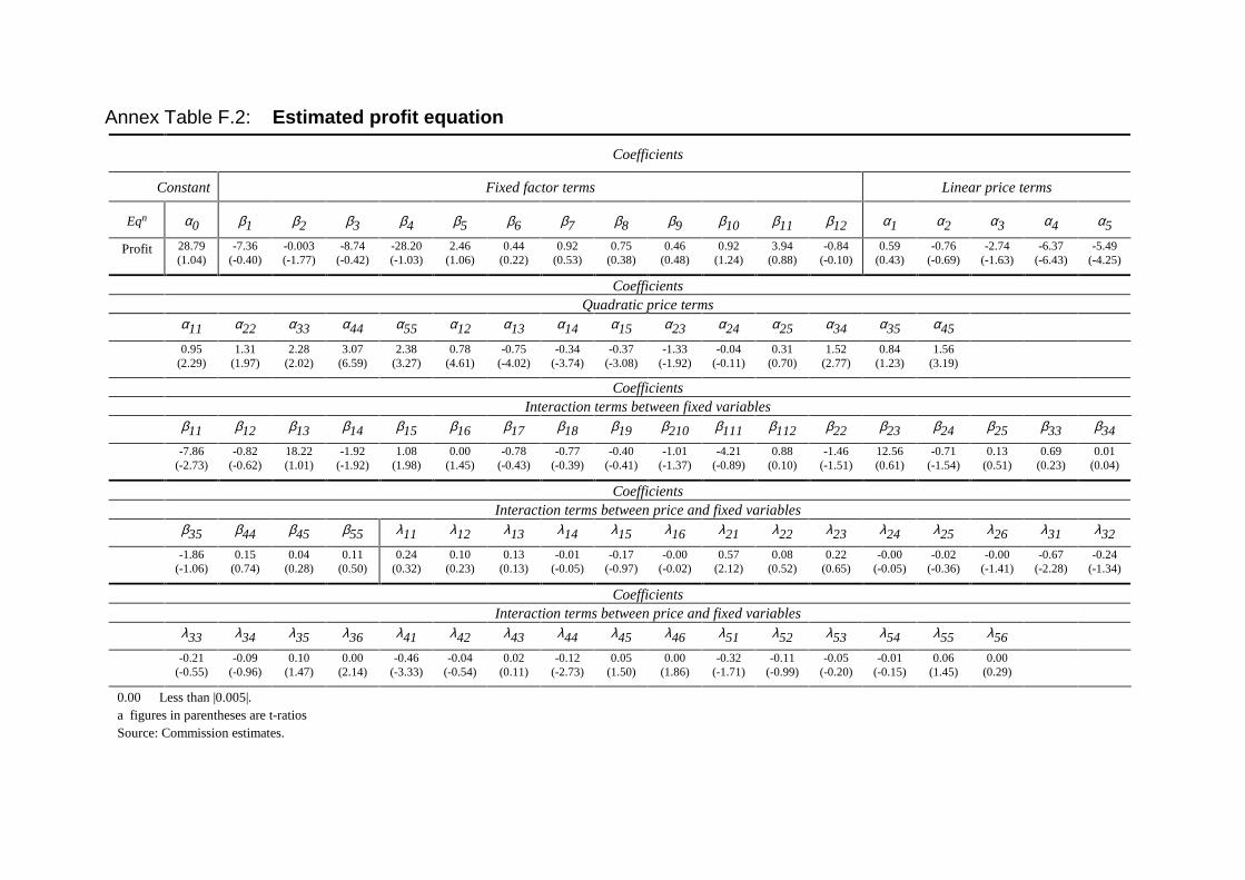
Annex Table F.2: Estimated profit equation
Coefficients
Constant Fixed factor terms Linear price terms
Eqn α0 β1 β2 β3 β4 β5 β6 β7 β8 β9 β10 β11 β12 α1 α2 α3 α4 α5
Profit 28.79(1.04)
-7.36(-0.40)
-0.003(-1.77)
-8.74(-0.42)
-28.20(-1.03)
2.46(1.06)
0.44(0.22)
0.92(0.53)
0.75(0.38)
0.46(0.48)
0.92(1.24)
3.94(0.88)
-0.84(-0.10)
0.59(0.43)
-0.76(-0.69)
-2.74(-1.63)
-6.37(-6.43)
-5.49(-4.25)
CoefficientsQuadratic price terms
α11 α22 α33 α44 α55 α12 α13 α14 α15 α23 α24 α25 α34 α35 α45
0.95(2.29)
1.31(1.97)
2.28(2.02)
3.07(6.59)
2.38(3.27)
0.78(4.61)
-0.75(-4.02)
-0.34(-3.74)
-0.37(-3.08)
-1.33(-1.92)
-0.04(-0.11)
0.31(0.70)
1.52(2.77)
0.84(1.23)
1.56(3.19)
CoefficientsInteraction terms between fixed variables
β11 β12 β13 β14 β15 β16 β17 β18 β19 β210 β111 β112 β22 β23 β24 β25 β33 β34
-7.86(-2.73)
-0.82(-0.62)
18.22(1.01)
-1.92(-1.92)
1.08(1.98)
0.00(1.45)
-0.78(-0.43)
-0.77(-0.39)
-0.40(-0.41)
-1.01(-1.37)
-4.21(-0.89)
0.88(0.10)
-1.46(-1.51)
12.56(0.61)
-0.71(-1.54)
0.13(0.51)
0.69(0.23)
0.01(0.04)
CoefficientsInteraction terms between price and fixed variables
β35 β44 β45 β55 λ11 λ12 λ13 λ14 λ15 λ16 λ21 λ22 λ23 λ24 λ25 λ26 λ31 λ32
-1.86(-1.06)
0.15(0.74)
0.04(0.28)
0.11(0.50)
0.24(0.32)
0.10(0.23)
0.13(0.13)
-0.01(-0.05)
-0.17(-0.97)
-0.00(-0.02)
0.57(2.12)
0.08(0.52)
0.22(0.65)
-0.00(-0.05)
-0.02(-0.36)
-0.00(-1.41)
-0.67(-2.28)
-0.24(-1.34)
CoefficientsInteraction terms between price and fixed variables
λ33 λ34 λ35 λ36 λ41 λ42 λ43 λ44 λ45 λ46 λ51 λ52 λ53 λ54 λ55 λ56
-0.21(-0.55)
-0.09(-0.96)
0.10(1.47)
0.00(2.14)
-0.46(-3.33)
-0.04(-0.54)
0.02(0.11)
-0.12(-2.73)
0.05(1.50)
0.00(1.86)
-0.32(-1.71)
-0.11(-0.99)
-0.05(-0.20)
-0.01(-0.15)
0.06(1.45)
0.00(0.29)
0.00 Less than |0.005|.a figures in parentheses are t-ratiosSource: Commission estimates.
STAFF INFORMATION PAPER
F26
Annex F2: Sources of data for the integrated econometricmodelling data base
Information necessary to undertake a broad economic analysis of agriculture and landdegradation is not available from a single source. Nevertheless, there is a range of sourcesthat individually have components of the information necessary to undertake the analysis.Information has been brought together from these various data bases to form the analyticaldata base used in this study.
The main series used in the analysis were obtained from ABS, ABARE and SCS-New SouthWales sources. For the current pilot study, the data assembled relate to the agriculturalindustry in New South Wales. As not all data from these sources are available for thereference years of the study, that is 1991–92 and 1992–93, the reference year for data usedand any adjustments to place it on a 1991–93 basis are described. With the exception ofinformation about the level of land degradation, the data sources discussed below could alsobe used to construct a similar data base for other years and for the agricultural sector in otherstates.
Economic data
Local value of commodities produced is the value of commodities at the place of production.It is estimated by deducting ex-farm marketing costs from the gross value of commoditiesproduced. Data on gross value of production classified by SLA were obtained from the ABSAgricultural Census. These values were generally converted to the required local value basisusing state-wide local value to gross value ratios obtained from ABS value of commoditiesproduced series (ABS Cat. No. 7503). For the commodities: barley, oats, wool, sheep andbeef cattle, local values were estimated on a regional basis using unit value information fromABARE farm finance surveys and the volume of production from the ABS AgriculturalCensus.
Volume indexes of commodities produced were estimated by revaluing current pricecommodity production series (at local values) derived from ABS production data by ABAREcommodity price indexes. The series were revalued to constant 1991–92 dollars. In a secondstage, individual commodity flows were aggregated to the broad commodity groups used inthe analysis, namely, crops and plant products and animals and animal products. Theinformation was used to estimate aggregate indexes of commodities produced. An index with1991–92=100 was then estimated from the series of values.
Price indexes of commodities produced were estimated for each SLA by reweighting theABARE indexes of prices received by farmers in New South Wales by the level of productionof each commodity in 1991-92. The price index used is therefore a fixed weighted (orLaspeyres) price index. The base period of the price index is 1991–92=100. In the analysis,output prices are lagged one period to indicate that farmers’ land management decisions for
APPENDIX F: ESTIMATES OF THE EFFECTS OF LAND DEGRADATION IN NEW SOUTH WALES
F27
the year are based on prices received in the previous year. This approach conforms to theapproach adopted in comparable studies (see Section F.3).
The area of agricultural land holdings and the area of irrigated land was obtained for eachSLA from the annual Agricultural Census conducted by the ABS.
The number of farmers and farm managers were obtained by SLA from the 1991 PopulationCensus conducted by the ABS.
Industry costs were estimated for each SLA using a three stage process. First, industry coststructures were obtained from Agricultural Finance Survey data published by the ABS (Cat.No. 7507.0) and farm financial information obtained from ABARE farm surveys (ABAREvarious). In many cases, relevant industry data were available for the study reference years of1991-92 and 1992-93. These data were used directly in the analysis. In some cases, relevantinput cost data were only available for other years. These data were adjusted to a 1991–92 or1992–93 basis, as appropriate, using an index of prices paid by New South Wales farmersobtained from ABARE (1995b). For some items, such as water, there was no price dataavailable at the time of estimation. A general price index was used to calculate water costs.In the second stage, each agricultural commodity produced in each SLA was matched to anindustry cost structure and an implicit cost structure for the production of that commodity inthe SLA was estimated. Thirdly, the costs for the SLA were obtained by aggregating the costspertaining to commodities produced. Finally, the costs for each SLA were summarised intothe groups: labour costs, fertiliser costs, water costs (including water rates), and othermaterials and service inputs. Once the estimation process was complete, indexes of currentprice inputs were estimated, with the base year being 1991–92=100.
The number of persons employed as hired labour were estimated by dividing wages andsalaries paid by farm industries by a farm labour wage rate.
Implicit indexes of the volume of intermediate inputs to the production of agriculturalcommodities were estimated by revaluing input costs to 1989–90 prices using ABAREindexes of prices paid by farmers in NSW (ABARE, 1995b). The estimated constant 1989–90price inputs were linked to SLA and then aggregated to summary commodity using theprocedure applied to current price inputs (see above). Indexes of intermediate inputs toproduction were then estimated for each SLA, with the base year being 1991–92=100.
Indexes of prices paid for inputs by SLA were estimated by dividing the index of current priceinputs by the index of constant price inputs with 1991–92=100.
Farm operating surplus (the model estimate of profit) is estimated for each SLA by deductinglabour income and intermediate input costs from an estimate of income from farm production.
Land degradation and other environmental data
An index of land degradation by type of degradation was estimated for each SLA fromapproximately 13000 grid points assessed in the Land Degradation Survey, NSW 1987–1988.

STAFF INFORMATION PAPER
F28
The grid point data were provided on disk by the SCS-New South Wales and linked to SLAsusing GIS techniques by the National Resource Information Centre (NRIC), Bureau ofResource Sciences. An assessment of land degradation in New South Wales using data fromthis survey is provided in Appendix C. Because degradation advances slowly, the 1987–1988data were used as a proxy for the level of degradation prevailing in the 1991 to 1993 period.
REFERENCES 1
REFERENCES
AACM 1995, Social and Economic Feasibility of Ameliorating Soil
Acidification, Land and Water Resources RDC, Canberra.
ABARE 1994, Commodity Statistical Bulletin, ABARE, Canberra.
—— 1995a, Commodity Statistical Bulletin, Supplementary price index data forNew South Wales farms provided on disk, ABARE, Canberra.
—— 1995b, The Land Care Taxation Provisions — Some Issues, in Outlook1995, ABARE, Canberra.
—— various, Farm Survey Data on Microfiche and Data Disk, ABARE,Canberra.
ABS 1983, Selected Agricultural Commodities, Australia 1982–83
(Preliminary) (Cat. No. 7112.0), Canberra.
—— 1988, Selected Agricultural Commodities, Australia, 1987-88, Preliminary(Cat. No. 7112.0), Canberra.
—— 1990, Projections of the Populations of Australia, States and Territories
1989 to 2031 (Cat. No. 3222.0), Canberra.
—— 1994, 1989-90 Australian National Accounts Input-output tables
(Cat. No. 5209.0), Canberra.
—— 1995a, Year Book, Australia 1995 (Cat. No. 1301.0), AGPS, Canberra.
—— 1995b, Cost of Environmental Protection, Selected Industries, 1991–92
(Cat. No. 4603.0), AGPS, Canberra.
—— 1995c, National Income, Expenditure and Product, Australian National
Accounts, September Quarter 1995 (Cat. No. 5206.0), Canberra.
—— 1995d, Small Area Agricultural Commodity Data (Agstats)(Cat. No. 7119.0), Canberra.
—— 1995e, Data provided on the estimated area of each New South WalesSLA, Special Request, Canberra.
STAFF INFORMATION PAPER
REFERENCES 2
—— (various), Australian National Accounts Capital Stock (Cat. No. 5221.0),Canberra.
—— (various), Australian National Accounts National Income, Expenditure
and Product (Cat. No. 5204.0), Canberra.
Adams, P.D. 1987, Agricultural Supply Response in ORANI, Review ofMarketing and Agricultural Economics, 55:213-29.
Australian Nature Conservation Agency (ANCA) (1995), Concordance Between
SLA and Biogeographic Region, Data provided on disk.
Australian Soil Conservation Council (undated), National Soil Conservation
Strategy, AGPS, Canberra.
Bullen, F. 1995, in Graetz R.D., Wilson M.A. and Cambell S.K. 1995,Landcover Disturbance Over the Australian Continent: a Contemporary
Assessment, Biodiversity series, Paper No. 7, Biodiversity Unit,Department of Environment, Sport and Territories, Canberra.
Bureau of Resource Sciences (BRS) 1995, Processing of CaLMs Data in GIS
Framework, Canberra.
Campbell, C. 1994, “Economics of Salinity Management for a Catchment inWestern Australia”, in Webb A A and Price R J 1994, Procedures for
Economic Assessment of Management Options for Dryland Salinity:
Report on a Workshop, Land and Water Resources RDC Occasional PaperSeries No. 6/94, Canberra.
Clarke, H.R. 1992, The Supply of Non-degraded Agricultural Land, AustralianJournal of Agricultural Economics, Vol. 36, No. 1, April 1992.
Commission of the European Communities (CEC), International Monetary Fund(IMF), Organisation for Economic Cooperation and Development(OECD), United Nations (UN), and the World Bank 1993, System of
National Accounts 1993, Brussels/Luxembourg, New York, Paris,Washington.
Commonwealth of Australia 1991, Decade of Landcare Plan: Commonwealth
Component, Commonwealth of Australia, Canberra.
REFERENCES
REFERENCES 3
—— 1992, National Strategy for Ecologically Sustainable Development, AGPS,Canberra.
Commonwealth Scientific and Industrial Organisation (CSIRO) 1995, Weeding
Out Woody Invaders, in Coping with Climate, Ecos 84, Winter 1995.
Conservation and Land Management (CaLM) 1995, 1987–1988 SCS-New South
Wales Land Degradation Survey, Data provided on Disk.
Coxhead, I.A. 1988, Estimating Factor Demand Elasticities for Philippine
Agriculture, paper presented at the 1988 Australian Economic Congress,28 August - 2 September, Canberra.
Cullen, P. and Bowmer, K. 1995, Agriculture, Water and Blue Green Algal
Blooms, in Sustaining the Resource Base, Prime Minister’s Science andEngineering Council, AGPS, Canberra.
Dee, P., Geisler, C. and Watts, G. 1996, The Impact of APEC’s Free Trade
Commitment, Staff Information Paper, AGPS, Canberra.
Department of Agriculture (Western Australia) 1988, "Situation Statement, Soiland Land Conservation Program In Western Australia", Departmental
Submission to the House of Representatives Inquiry into Land
Degradation, Perth.
Department of Environment, Sport and Territories (DEST) 1995a, A Profile,Department of Environment, Sport and Territories, Canberra.
—— 1995b, Native Vegetation Clearance, Habitat Loss and Biodiversity
Decline, Biodiversity Series, Paper No. 6, Biodiversity Unit, Departmentof Environment, Sport and Territories, Canberra.
Department of Primary Industries and Energy Industry (undated), Income
Taxation Deductions for Landcare Related Activities, brochure preparedby the Department of Primary Industries and Energy in consultation withthe Australian Taxation Office and State and Territory GovernmentDepartments, Canberra.
Dewbre, J., Shaw, I., and Corra, G. 1985, The EMABA Model - Structure,
Specifications and Some Results, BAE Occasional Paper, AGPS,Canberra.

STAFF INFORMATION PAPER
REFERENCES 4
Diewert, W.E. and Wales, T.J. 1987, Flexible Functional Forms and Global
Curvature Conditions, Econometrica, 55(1):43-68.
Ecologically Sustainable Development Working Group-Agriculture 1991, Final
Report—Agriculture, AGPS, Canberra.
Environment Protection Authority New South Wales 1993, New South Wales
State of the Environment 1993 Chatswood.
Evans, G. 1991, Acid Soils in Australia: The Issues for Government, Bureau ofRural Resources, Canberra.
Graham, O.P. 1989, Land Degradation Survey of New South Wales 1987–1988:
Methodology, SCS Technical Report No. 7, Soil Conservation Service ofNSW, Chatswood.
Graetz R.D., Wilson M.A. and Cambell S.K. 1995, Landcover Disturbance
Over the Australian Continent: a Contemporary Assessment, Biodiversityseries, Paper No. 7, Biodiversity Unit, Department of Environment, Sportand Territories, Canberra.
Grice, M.S. 1995, Assessment of Soil and Land Degradation on Private
Freehold Land in Tasmania, Department of Primary Industry andFisheries, Tasmania
Gutteridge, Haskins & Davey et al. 1990, Pipeline to the Sea: Pre-feasibility
Study, Report for Murray Darling Basin Commission, Canberra.
Hamblin, A. and Williams, J. 1995, Soils: Key Issues in Sustaining the Land
Resource Base, in Sustaining the Resource Base, Prime Minister’s Scienceand Engineering Council, AGPS, Canberra.
Hamblin, A. and Kyneur, G. 1993, Trends in Wheat Yields and Soil Fertility in
Australia, AGPS, Canberra.
Helyar, K.R., Cregan, P.D. and Godyn, D.L. 1990, Soil acidity in NSW—current pH values and estimates of acidification rates, Australian Journal
of Soil Resources, 28, p.3–37.
Hertel, T.W. 1990, Applied General Equilibrium Analysis of Agricultural
Policies, Staff paper No 90-9, Purdue University.
REFERENCES
REFERENCES 5
Hufschmidt, M.M., James, D.E., Meister, A.D., Bower, B.T. and Dixon, J.A.1983, Environment, Natural Systems, and Development: an Economic
Valuation Guide, Johns Hopkins University Press, Baltimore.
Humphries S.E., Groves, R.H. and Mitchell, D.S. 1991, Plant Invasions: the
Incidence of Environmental Weeds in Australia, Kowari 2, an AustralianNational Parks and Wildlife Service Publication, Canberra.
Huthwaite, Peter 1995, ‘Incentives for Landcare’, in Outlook 95, Proceedings of
the National Agricultural Outlook Conference, Canberra 7–9 February1995, AGPS, Canberra.
Industry Commission 1993, Annual Report 1992–93, AGPS, Canberra.
—— 1994, Annual Report 1993–94, AGPS, Canberra.
—— 1995, Annual Report 1994–95, AGPS, Canberra.
—— 1995a, Research and Development, Report No. 44, AGPS, Canberra.
—— 1995b, Government Support to R&D by Benefiting Industry, Paper
Prepared by the Industry Commission for Its Inquiry into Research and
Development (Report No. 44), Canberra.
International Union for Conservation of Nature and Natural Resources (IUCN)1980, World Conservation Strategy—Living Resource Conservation for
Sustainable Development, prepared by IUCN with advice and assistancefrom UNEP, WWF and in collaboration with FAO and UNESCO, Morges,Switzerland.
James, D.E. 1994, The Application of Economic Techniques in Environmental
Impact Assessment, Environmental Management Volume 4, KluwerAcademic Publishers, Dordrecht
Johnson, D.L. and Lewis, L.A. 1995, Land Degradation: Creation and
Destruction, Blackwell, Oxford.
Jorgenson, D.W. and Fraumeni, B.M. 1981, Relative Prices and Technical
Change, in E.R. Berndt and B.C. Field (eds), Modelling and MeasuringNatural Resource Substitution, MIT Press, Cambridge, Massachusetts: 17-47.

STAFF INFORMATION PAPER
REFERENCES 6
Kaleski, L.G. 1945, The Erosion Survey of NSW, Journal of Soil ConservationService of NSW, October 1963.
Keating, P.J. 1995, Our Land Statement, Speech by the Prime Minister, Albury24 January.
Land and Water RDC 1995, Data Sheets on Natural Resource Issues,Occasional Paper No. 06/95, Land and Water RDC, Canberra.
Land and Water RDC, National Soil Conservation Program, and Murray-Darling Basin Commission 1992, Dryland Salinity R&D, PDP AustraliaPty Ltd.
Lau, L.J. 1976, A Characterization of the Normalized Restricted Profit
Function, Journal of Economic Theory, 12:131-63.
_____ 1978, Testing and Imposing Monotonocity, Convexity and
Quasiconvexity Constraints, in M. Fuss and D. McFadden (eds),Production Economics: a dual approach to theory and applications, Vol. 1,North-Holland Publishers, Amsterdam :409-54.
Lawrence, D. and Zeitsch, J. 1989, A Disaggregated Model of Australian
Agricultural Production Response, contributed paper presented to 33rdannual conference of the Australian Agricultural Economic Society,Christchurch, New Zealand.
_____ 1989b, Estimating Generalised McFadden Profit and Aggregation
Functions for Australian Agriculture, Industries Assistance Commission,Canberra.
Lawrence, D. 1990, A Generalised McFadden for Australian Agriculture,
contributed paper presented to 34th annual conference of the AustralianAgricultural Economic Society, Brisbane.
Legislative Assembly, Western Australia 1991, Select Committee into Land
Conservation, Final Report, Perth.
Maligaya, A.R. and White, F.C. 1989, Agricultural Output Supply and Input
Demand Relationships with Endogenous Land Rents, Southern Journal ofAgricultural Economics, December, 1989, 13-20.
REFERENCES
REFERENCES 7
Mallawaarachchi, T., Young, M., Walker, P., and Smyth, B. 1994, Economic
Assessment of Land Management Options: a GIS-based Natural Resource
Accounting Approach, in Procedures for Economic Management Options
for Dryland Salinity, Report of workshop, Occasional Paper No. 6/94,Land and Water Resources RDC, Canberra.
Mallawaarachchi, T., Young, M. 1994, Economic Costs of Land Degradation:
Assessment, Analysis and Policy Implications, Paper presented at the 38thannual conference of the Australian Agricultural Economics Society,Victoria University, Wellington, New Zealand, February 1994.
Marshall, G., Jones, R. and McGrath, S. 1994, Significance of Farmer Response
for Estimating Agricultural Costs of Land Salinisation, Paper presented tothe 39th Conference of the Agricultural Economics Society, Wellington,New Zealand, February 1994.
McKay, L., Lawrence, D. and Vlastuin, C. 1980, Input Demand and
Substitution in the Australian Sheep Industry, Review of Marketing andAgricultural Economics, 48(2):57-70.
_____ 1983, Profit, Output Supply, and Input Demand Functions for
Multiproduct Firms: the Case of Australian Agriculture, InternationalEconomic Review, 24(2):323-39.
McTainsh G.H., and Boughton W.C. 1993, Land Degradation Processes in
Australia, Longman Cheshire, Melbourne.
Moschini, G. 1988, A Model of Production with Supply Management for the
Canadian Agricultural Sector, American Journal of AgriculturalEconomics, 70(2):318-29.
Murray-Darling Basin Ministerial Council (MDBMC) 1987, Salinity and
Drainage Strategy, Background Paper No. 87/1, Canberra.
National Resource Information Centre (NRIC) 1995, Processing of CaLMs
Data in GIS Framework, Bureau of Resource Sciences, Canberra.
National Soil Conservation Council (undated), National Soil Conservation
Strategy, AGPS, Canberra.
STAFF INFORMATION PAPER
REFERENCES 8
Nehring, R.F. 1991, Output and Input Subsidy Policy Options in Bangladesh,Journal of Agricultural Economics Research, Vol 43(2), spring 1991, 29-41.
Office of the Commissioner of the Environment-Victoria 1991, 1991 State of
the Environment Report, Agriculture and Victoria’s Environment,Government of Victoria, Melbourne.
Oram, D. and Dumday, R. 1994, ’Evaluating the Benefits and Costs of DrylandSalinity Control at the Farm Level: a Case Study in the CampaspeCatchment’, in Webb A.A. and Price R.J. 1994, Procedures for Economic
Assessment of Management Options for Dryland Salinity: Report on a
Workshop, Land and Water Resources RDC Occasional Paper Series No.6/94, Canberra.
Pagiola, S. 1993, Soil Conservation and the Sustainability of Agricultural
Production, A dissertation submitted to the Food Research Institute andthe Committee on Graduate Studies of Stanford University in partialfulfilment of the requirements for a degree of doctor of philosophy.
Pearce, D.W. and Turner, R.K. 1990, Economics of Natural Resources and the
Environment, Harvester Wheatshef, New York.
Perkins, F.C. 1994, Practical Cost Benefit Analysis, Macmillian Educational.
Peterson, W. 1979, International Farm Prices and the Social Costs of Cheap
Food Policies, American Journal of Agricultural Economics, Vol61(1):12-21.
Polson, R.A. and Shumway, C.R., 1992, Production Relationships in South
Central Agriculture, Southern Journal of Agricultural Economics,December, 1992, 121-35.
Porter, W.M. and McLaughlin, M.J. 1992, Evaluation of the Use of Agricultural
Lime in Australia, Report for the Grains R&D Corporation.
Salma, U. 1992, Production Technology and Allocation Decisions in
Agriculture: Bangladesh, Economic Division Working Paper No 92/3,Research School of Pacific Studies, Australian National University,Canberra.
REFERENCES
REFERENCES 9
Shumway, C.R., Saez, R.R. and Gottret, P.E. 1988, Multiproduct Supply and
Input Demand in US Agriculture, American Journal of AgriculturalEconomics, 70(2):330-37.
Soil Conservation Service of NSW 1989, Land Degradation Survey, New South
Wales 1987–1988, Soil Conservation Service of NSW, Chatswood.
Stewart, J. 1968, Erosion Survey of New South Wales Eastern and CentralDivisions Re-Assessment–1967, Journal of the Soil Conservation Service
of NSW, Vol. 24(3), July 1968.
Sweeney, J.L. 1993, Economic Theory of Depletable Resources: an
Introduction, in Handbook of Natural Resource and Energy Economics,Knees, A.V. and Sweeny, J.L. (Editors), Elsevier, Amsterdam.
Thackway, R. and Cresswell, I.D. (Editors) 1995, An Interim Biogeographic
Regionalisation for Australia: a Framework for Establishing the National
System of Reserves, Version 4.0, Australian Nature Conservation Agency,Canberra.
Tothill J.C. and Gillies C. 1992, The Pasture Lands of Northern Australia:
Their Condition, Productivity, and Sustainability. Report prepared for theMeat Research Corporation, Tropical Grasslands Society of Australia,Occasional Publication No. 5, Brisbane.
United Nations Conference on the Environment 1992, Agenda 21 Program of
Action for Sustainable Development: Rio Declaration on the Environment
and Development, UNCED, Rio de Janeiro.
Vincent, D.P., Dixon, P.B. and Powell, A.A. 1980. The Estimation of Supply
Response in Australian Agriculture: the CRESH/CRETH Production
System, International Economic Review, 21(1):221-242.
Wall, C.A., and Fisher, B.S. 1987, Modelling a Multiple Output Production
System: Supply Response in the Australian Sheep Industry, ResearchReport No 11, Department of Agricultural Economics, University ofSydney.
STAFF INFORMATION PAPER
REFERENCES 10
_____ 1990, Supply Response in the Australian Sheep Industry: a Profit
Function Approach, Australian Journal of Agricultural Economics, Vol34(2):147-66.
Walpole, S.C., Sinden, J.A., and Yapp, T.P. 1992, The Opportunity Cost of
Land Degradation on Agriculture in New South Wales, Department ofAgriculture and Business Management, University of New England, andNew South Wales Department of Conservation and Land Management.Armidale and Sydney.
White, K.J. 1978, A General Computer Program for Econometric Methods -
SHAZAM, Econometrica, Vol 46(1):239-40.
Wicks, J.A. and Dillon, J.L. 1978, APMAA Estimates of Supply Elasticities for
Australian Wool, Beef and Wheat, Review of Marketing and Agriculturaleconomics, Vol 46: 48-57.
Wiley, D.E., Schmidt, W.H. and Bramble, W.J. 1973, Studies of a Class of
Covariance Structure Models, Journal of the American StatisticalAssociation, Vol 68(342):317-23.
Woods, L.E. 1983, Land Degradation in Australia, Australian EnvironmentStatistic Project, Department of Home Affairs and Environment, Canberra.
World Commission on Environment and Development (1987), Our Common
Future, OUP, Oxford.