laboratory measurements of porosity, permeability ... · pdf filelaboratory measurements of...

La

C

emf�p�1hnPflat

c

U

©

GEOPHYSICS, VOL. 75, NO. 6 �NOVEMBER-DECEMBER 2010�; P. E191–E204, 14 FIGS., 5 TABLES.10.1190/1.3493633

aboratory measurements of porosity, permeability, resistivity,nd velocity on Fontainebleau sandstones

armen T. Gomez1, Jack Dvorkin2, and Tiziana Vanorio2

s4dF1ptstdts1l

ABSTRACT

The relations among the resistivity, elastic-wave velocity, po-rosity, and permeability in Fontainebleau sandstone samplesfrom the Ile de France region, around Paris, France were experi-mentally revisited. These samples followed a permeability-po-rosity relation given by Kozeny-Carman’s equation. For the re-sistivity measurements, the samples were partially saturated withbrine. Archie’s equation was used to estimate resistivity at 100%water saturation, assuming a saturation exponent, n�2. Usingself-consistent �SC� approximations modeling with grain aspectratio 1, and pore aspect ratio between 0.02 and 0.10, the experi-mental data fall into this theoretical range. The SC curve with thepore aspect ratio 0.05 appears to be close to the values measuredin the entire porosity range. The elastic-wave velocity was mea-

rw

tiTt�tdpcti

ived 12aliforni

.A. E-m

E191

Downloaded 04 Jul 2011 to 128.194.170.136. Redistribution subject to

ured on these dry samples for confining pressure between 0 and0 MPa.Aloading and unloading cycle was used and did not pro-uce any significant hysteresis in the velocity-pressure behavior.or the velocity data, using the SC model with a grain aspect ratioand pore aspect ratios 0.2, 0.1, and 0.05 fit the data at 40 MPa;ore aspect ratios ranging between 0.1, 0.05, and 0.02 were a bet-er fit for the data at 0 MPa. Both velocity and resistivity in cleanandstones can be modeled using the SC approximation. In addi-ion, a linear fit was found between the P-wave velocity and theecimal logarithm of the normalized resistivity, with deviationshat correlate with differences in permeability. Combining thetiff sand model and Archie for cementation exponents between.6 and 2.1, resistivity was modeled as a function of P-wave ve-ocity for these clean sandstones.

INTRODUCTION

Velocity and resistivity of rocks depend on porosity, texture, min-ralogy, and pore fluid. Some of the earliest laboratory measure-ents showing the variation of the acoustic properties of rocks as

unctions of porosity, saturation, and pressure were by Wyllie et al.1956, 1958�. These studies showed that porosity undoubtedly is therimary factor affecting P- and S- wave velocities. Later studiesNur and Simmons, 1969; Domenico, 1976; Mavko, 1980; Murphy,984� have refined our understanding of rock properties showingow pore type and pore fluid distribution �i.e., saturation heteroge-eity� may contribute to variations in the P- and S- wave velocities.ore geometry, in particular, affects pore stiffness which, in turn, in-uences the velocity sensitivity to pressure �Mavko, 1980; Mavkond Nur, 1978; O’Connell and Budiansky, 1974� as well as to satura-ion �Mavko and Mukerji, 1995�.

Similarly, Archie �1942� was the first to show that the ratio of theonductivity of the pore fluid to the bulk conductivity of fully-satu-

Manuscript received by the Editor 4August 2009; revised manuscript rece1Formerly Stanford University, Department of Geophysics, Stanford, C

.S.A. E-mail: [email protected] University, Department of Geophysics, Stanford, California, U.S2010 Society of Exploration Geophysicists.All rights reserved.

ated and clean sandstones corresponds to the formation factor F,hich is related to porosity through the following relation:

F�a

�m �1�

The m and a coefficients, known as the cementation exponent andortuosity factor, are usually determined empirically. In equation 1, as close to 1, and was first introduced by Wyllie and Gregory �1953�.he a coefficient may be considered a reservoir constant according

o Worthington �1993�, although originally Wyllie and Gregory1953� considered it a function of porosity and formation factor ofhe original unconsolidated aggregate before cementation. When theominant electrical conduction mechanism is ionic diffusion in theore fluid, as in the case of clean, well-sorted sands, a has to be 1, be-ause as porosity tends to 1, the conductivity of the rock is equal tohe conductivity of the fluid �Mavko et al., 1998�. The coefficient ms also called the porosity exponent and different studies have related

May 2010; published online 3 November 2010.a; presently Shell Exploration and Production Company, Houston, Texas,

ail: [email protected]; [email protected].

SEG license or copyright; see Terms of Use at http://segdl.org/

ictfmt�rtftspg

va�stfseffpRt

ccttartSa

tr

tg2wmvm

Tscot0tsAti

ct�

0aTr

tm4bpateti�

Gsbe

lHwMss

Fr

E192 Gomez et al.

t to grain and pore shape �Jackson et al., 1978; Ransom, 1984�. Ac-ording to Knight and Endres �2005�, m depends on the geometry ofhe system or the connectedness of the pore space, and is often re-erred to as the cementation factor because of the importance of ce-entation in determining microgeometry. The m coefficient is close

o 2 in sandstones, but it can be as high as 5 in carbonate rocksMavko et al., 1998�. The dependency of the a and m coefficients onock properties has been the subject of multiple studies �see Wor-hington, 1993 for a review�. Such studies report a large number ofactors affecting those constants, including porosity, type of porosi-y, tortuosity, pore geometry, degree of cementation, sorting, grainhape, packing of grains, pressure, and wettability. Schön �1996� re-orts that both parameters, a and m, are controlled by pore channeleometry, including pore shape and connectivity.

In this study, we measure porosity, permeability, resistivity, andelocity in Fontainebleau sandstones. We first examine the perme-bility — porosity relation, and compare it to the Kozeny-CarmanCarman, 1961� relation, and a previous study by Bourbie and Zin-zner �1985�. We then analyze how porosity and permeability relateo resistivity using effective medium models, such as differential ef-ective medium �DEM� �Bruggeman, 1935; Berryman, 1995� andelf-consistent �SC� �Landauer, 1952; Berryman, 1995�, and a semi-mpirical model by Archie �1942�. We follow a similar procedureor P-wave and S-wave velocities as a function of porosity, using ef-ective medium models, including also DEM and SC, and semi-em-irical models, including the stiff sand model �Gal et al., 1998�, theaymer-Hunt-Gardner relation �Raymer et al., 1980�, and Wyllie’s

ime-average equation �Wyllie et al., 1958�.Elastic and electrical methods can contribute in different ways to

haracterizing rock. Each of them has limitations that can be over-ome by integration with the other. The literature shows that labora-ory studies performing joint measurements and analysis of veloci-ies and resistivity of sedimentary rocks are quite scarce �i.e., Polaknd Rapoport, 1956, 1961; Parkhomenko, 1967; Knight, 1991; Car-ara et al., 1999.All these studies only use P-wave velocity and resis-ivity�. In particular, there are no laboratory studies that use P-,-wave velocities and resistivity together to better estimate porositynd permeability of reservoir rocks. Therefore, we examine the rela-

Helium porosity (%)

Tot

alpo

rosi

ty(%

)

30

25

20

15

10

5

00 5 10 15 20 25 30

igure 1. Total porosity estimated from volume and mass versus po-osity measured using helium porosimeter.


ion between resistivity and velocity, and how these two propertieselate to porosity and permeability.

METHOD

The set of core plugs in this study comprises 23 Oligocene Fon-ainebleau sandstones, collected at outcrops in the Ile de France re-ion, around Paris, France. The core plugs have a diameter around.5 cm, and a length ranging between 2.3 and 3.9 cm. Resistivityas measured at 1 kHz at benchtop conditions using the 4-electrodeethod, with the benchtop set-up that is part of the Core Lab’s Ad-

anced Resistivity System Model 300. The instrumental error for theeasured resistivities is �10%.Core plugs were saturated with a 40,000 ppm NaCl solution.

heir water resistivity was monitored for a 48-hour period before theaturated rock resistivity measurements were performed to reach ahemical equilibrium between the rock and the fluid. The resistivityf water was monitored before performing each measurement. Theemperature of the water was 21�1 °C, and its resistivity.17�0.01 ohm·m. Water saturation of 100% was not reached forhese samples, particularly the low-porosity ones, with an averageaturation of 80%, the latter determined by weighing the samples.rchie’s equation was used to estimate the resistivities at full satura-

ion �R0� from the measured resistivity �Rt� at saturation SW assum-ng a saturation exponent �n� of 2, as it follows in equation 2:

R0�RtSWn �2�

This saturation exponent value is consistent with previous publi-ations, such as that by Durand �2003�, who measured three Fon-ainebleau samples with different porosities and found an average n

1.96.If we assume an error in n of 10%, the error in R0 is around 4%, or

.6 ohm·m. Sample A82 has the largest error of around 3 ohm·m,nd sample H27 has the smallest error in R0 of around 0.03 ohm·m.hese errors are a function of saturation, porosity, and the measured

esistivity.For 9 of the 23 core plugs, measurements of P- and S-wave veloci-

y were also performed under variable confining pressure, at one at-osphere pore pressure. Confining pressure was increased to

0 MPa, with 5 MPa increments. The plugs were jacketed with rub-er tubing to isolate them from the confining pressure medium. Theulse transmission technique was used to measure P-wave velocityt 1 MHz frequency and S-wave velocity at 0.7 MHz. The error forhe velocity measurements is around �1%. Three linear potentiom-ters were used to measure length changes of the samples as a func-ion of stress. These length changes were related to changes in poros-ty by assuming that pore contraction was the main cause of straini.e., we assume that the mineral was incompressible�.

Velocity measurements were performed at dry conditions. We useassmann’s �1951� fluid substitution to predict the velocities at full

aturation. This was to avoid velocity dispersion effects that woulde associated with fluid saturated ultrasonic measurements �Mavkot al., 2009�.

Helium porosity, Klinkenberg-corrected nitrogen permeability,ength, diameter and weight of all these plugs were also measured.elium porosity and total porosity estimated from volume andeight are essentially the same, as we can observe from Figure 1.ineralogy of these samples is 100% quartz, with an average grain

ize of 250 micrometers �Bourbie and Zinszner, 1985� �see also CTcan sections in Figure 2�. All the measurements are included in Ta-


bfA

pavps2iwq2

tp

wira

FH577

TR„

S

A

A

A

A

A

A

A

B

B

B

B

B

F

G

G

G

G

G

H

H

H

F

F

Laboratory measurements on sandstones E193

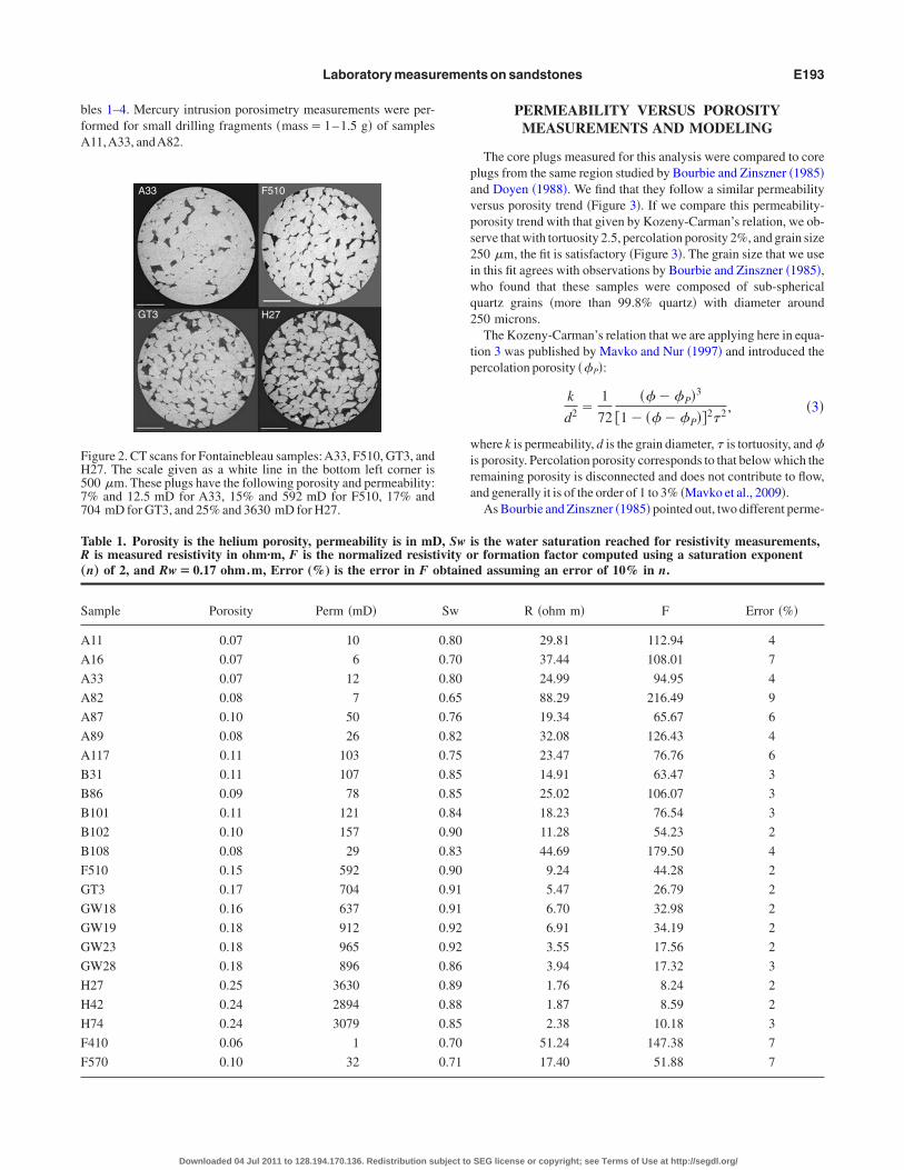
les 1–4. Mercury intrusion porosimetry measurements were per-ormed for small drilling fragments �mass�1–1.5 g� of samples11,A33, andA82.

A33 F510

GT3 H27

igure 2. CT scans for Fontainebleau samples: A33, F510, GT3, and27. The scale given as a white line in the bottom left corner is00 �m. These plugs have the following porosity and permeability:% and 12.5 mD for A33, 15% and 592 mD for F510, 17% and04 mD for GT3, and 25% and 3630 mD for H27.

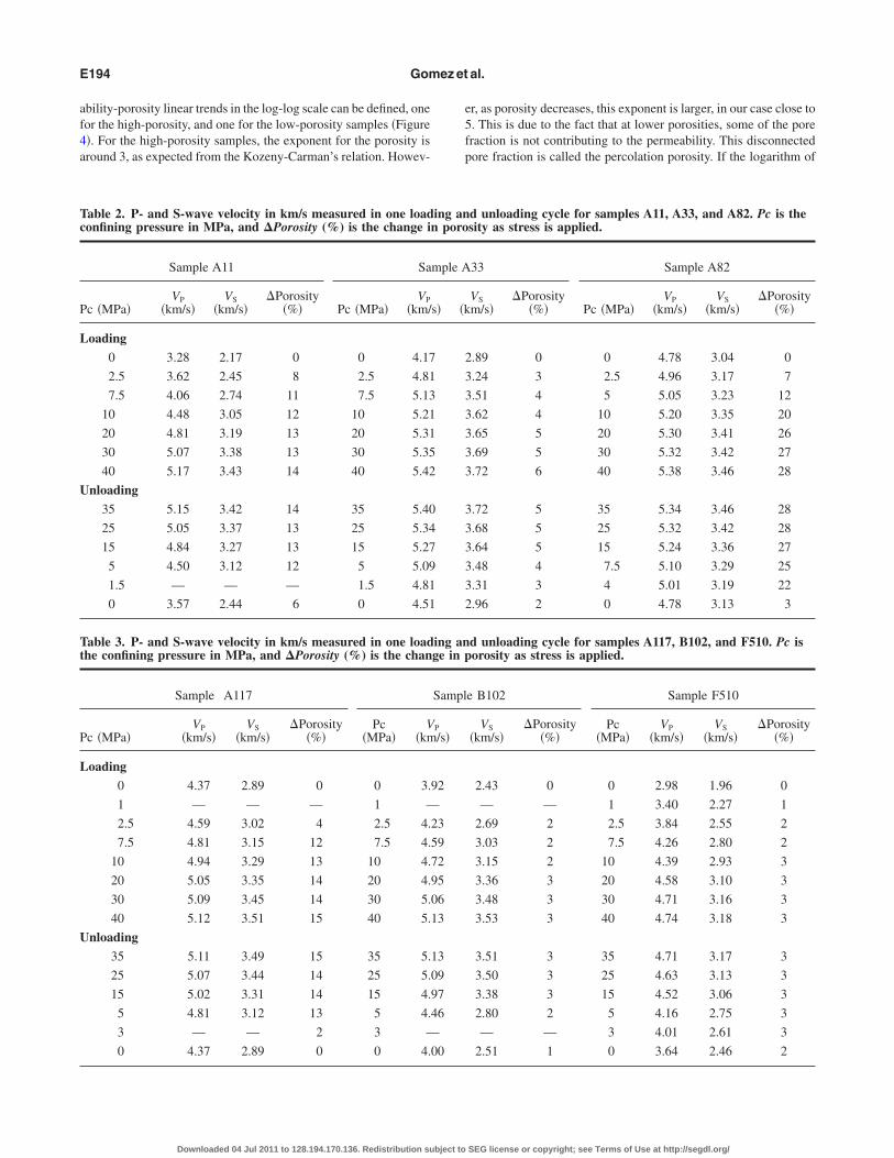
able 1. Porosity is the helium porosity, permeability is in mDis measured resistivity in ohm·m, F is the normalized resist

n… of 2, and Rw�0.17 ohm.m, Error (%) is the error in F o

ample Porosity Perm �mD�

11 0.07 10

16 0.07 6

33 0.07 12

82 0.08 7

87 0.10 50

89 0.08 26

117 0.11 103

31 0.11 107

86 0.09 78

101 0.11 121

102 0.10 157

108 0.08 29

510 0.15 592

T3 0.17 704

W18 0.16 637

W19 0.18 912

W23 0.18 965

W28 0.18 896

27 0.25 3630

42 0.24 2894

74 0.24 3079

410 0.06 1

570 0.10 32


PERMEABILITY VERSUS POROSITYMEASUREMENTS AND MODELING

The core plugs measured for this analysis were compared to corelugs from the same region studied by Bourbie and Zinszner �1985�nd Doyen �1988�. We find that they follow a similar permeabilityersus porosity trend �Figure 3�. If we compare this permeability-orosity trend with that given by Kozeny-Carman’s relation, we ob-erve that with tortuosity 2.5, percolation porosity 2%, and grain size50 �m, the fit is satisfactory �Figure 3�. The grain size that we usen this fit agrees with observations by Bourbie and Zinszner �1985�,ho found that these samples were composed of sub-sphericaluartz grains �more than 99.8% quartz� with diameter around50 microns.

The Kozeny-Carman’s relation that we are applying here in equa-ion 3 was published by Mavko and Nur �1997� and introduced theercolation porosity ��P�:

k

d2 �1

72

�� P�3

�1� �� P��2� 2 , �3�

here k is permeability, d is the grain diameter, � is tortuosity, and �s porosity. Percolation porosity corresponds to that below which theemaining porosity is disconnected and does not contribute to flow,nd generally it is of the order of 1 to 3% �Mavko et al., 2009�.

As Bourbie and Zinszner �1985� pointed out, two different perme-

is the water saturation reached for resistivity measurements,r formation factor computed using a saturation exponentd assuming an error of 10% in n.

R �ohm m� F Error �%�

29.81 112.94 4

37.44 108.01 7

24.99 94.95 4

88.29 216.49 9

19.34 65.67 6

32.08 126.43 4

23.47 76.76 6

14.91 63.47 3

25.02 106.07 3

18.23 76.54 3

11.28 54.23 2

44.69 179.50 4

9.24 44.28 2

5.47 26.79 2

6.70 32.98 2

6.91 34.19 2

3.55 17.56 2

3.94 17.32 3

1.76 8.24 2

1.87 8.59 2

2.38 10.18 3

51.24 147.38 7

17.40 51.88 7

, Swivity obtaine

Sw

0.80

0.70

0.80

0.65

0.76

0.82

0.75

0.85

0.85

0.84

0.90

0.83

0.90

0.91

0.91

0.92

0.92

0.86

0.89

0.88

0.85

0.70

0.71


af4a

e5fp

Tc

P

L

U

Tt

P

L

U

E194 Gomez et al.

bility-porosity linear trends in the log-log scale can be defined, oneor the high-porosity, and one for the low-porosity samples �Figure�. For the high-porosity samples, the exponent for the porosity isround 3, as expected from the Kozeny-Carman’s relation. Howev-

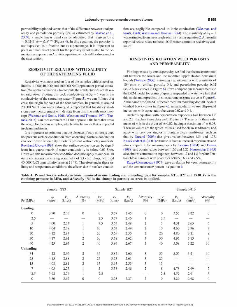
able 2. P- and S-wave velocity in km/s measured in one loadonfining pressure in MPa, and �Porosity (%) is the change i

Sample A11 Sa

c �MPa�VP

�km/s�VS

�km/s��Porosity

�%� Pc �MPa�VP

�km/

oading

0 3.28 2.17 0 0 4.17

2.5 3.62 2.45 8 2.5 4.81

7.5 4.06 2.74 11 7.5 5.13

10 4.48 3.05 12 10 5.21

20 4.81 3.19 13 20 5.31

30 5.07 3.38 13 30 5.35

40 5.17 3.43 14 40 5.42

nloading

35 5.15 3.42 14 35 5.40

25 5.05 3.37 13 25 5.34

15 4.84 3.27 13 15 5.27

5 4.50 3.12 12 5 5.09

1.5 — — — 1.5 4.81

0 3.57 2.44 6 0 4.51

able 3. P- and S-wave velocity in km/s measured in one loadhe confining pressure in MPa, and �Porosity (%) is the chan

Sample A117

c �MPa�VP

�km/s�VS


�%�Pc

�MPa�V

�km

oading

0 4.37 2.89 0 0 3.

1 — — — 1 —

2.5 4.59 3.02 4 2.5 4.

7.5 4.81 3.15 12 7.5 4.

10 4.94 3.29 13 10 4.

20 5.05 3.35 14 20 4.

30 5.09 3.45 14 30 5.

40 5.12 3.51 15 40 5.

nloading

35 5.11 3.49 15 35 5.

25 5.07 3.44 14 25 5.

15 5.02 3.31 14 15 4.

5 4.81 3.12 13 5 4.

3 — — 2 3 —

0 4.37 2.89 0 0 4.


r, as porosity decreases, this exponent is larger, in our case close to. This is due to the fact that at lower porosities, some of the poreraction is not contributing to the permeability. This disconnectedore fraction is called the percolation porosity. If the logarithm of

d unloading cycle for samples A11, A33, and A82. Pc is thesity as stress is applied.

33 Sample A82

VS

m/s��Porosity

�%� Pc �MPa�VP

�km/s�VS


�%�

2.89 0 0 4.78 3.04 0

3.24 3 2.5 4.96 3.17 7

3.51 4 5 5.05 3.23 12

3.62 4 10 5.20 3.35 20

3.65 5 20 5.30 3.41 26

3.69 5 30 5.32 3.42 27

3.72 6 40 5.38 3.46 28

3.72 5 35 5.34 3.46 28

3.68 5 25 5.32 3.42 28

3.64 5 15 5.24 3.36 27

3.48 4 7.5 5.10 3.29 25

3.31 3 4 5.01 3.19 22

2.96 2 0 4.78 3.13 3

d unloading cycle for samples A117, B102, and F510. Pc isorosity as stress is applied.

e B102 Sample F510

VS


�%�Pc

�MPa�VP

�km/s�VS


�%�

2.43 0 0 2.98 1.96 0

— — 1 3.40 2.27 1

2.69 2 2.5 3.84 2.55 2

3.03 2 7.5 4.26 2.80 2

3.15 2 10 4.39 2.93 3

3.36 3 20 4.58 3.10 3

3.48 3 30 4.71 3.16 3

3.53 3 40 4.74 3.18 3

3.51 3 35 4.71 3.17 3

3.50 3 25 4.63 3.13 3

3.38 3 15 4.52 3.06 3

2.80 2 5 4.16 2.75 3

— — 3 4.01 2.61 3

2.51 1 0 3.64 2.46 2

ing ann poro

mple A

s� �k

ing ange in p

Sampl

P

/s�

92

23

59

72

95

06

13

13

09

97

46

00


pr2�npmt

lttcc2scmti

ncRiHo4l

tSwrm

fb1�ttA�i

amTatKa�at

a

Tc

P

L

U


ermeability is plotted versus that of the difference between total po-osity and percolation porosity �2% as estimated by Mavko et al.,009�, a single linear trend can be identified that is given by k

0.0241�� P�3.792 �Figure 4�. In this equation, the porosity isot expressed as a fraction but as a percentage. It is important tooint out that this exponent for the porosity is not related to the ce-entation exponent in Archie’s equation, which will be discussed in

he next section.

RESISTIVITY RELATION WITH SALINITYOF THE SATURATING FLUID

Resistivity was measured on four of the samples with brine of sa-inities 11,000; 40,000; and 100,000 NaCl ppm under partial satura-ion. We applied equation 2 to compute the conductivities at full wa-er saturation. Plotting this rock conductivity at SW�1 versus theonductivity of the saturating water �Figure 5�, we can fit lines thatross the origin for each of the four samples. In general, at around0,000 NaCl ppm water salinity, it is expected that for shaley sand-tones any measurement will deviate from this line with zero inter-ept �Waxman and Smits, 1968; Waxman and Thomas, 1974; Tho-as, 2007�. Our measurement at 11,000 ppm still fits lines that cross

he origin for the four samples, which is the behavior that is expectedn clean sandstones.

It is important to point out that the absence of clay minerals doesot prevent surface conduction from occurring. Surface conductionan occur even when only quartz is present without clay minerals.evil and Glover �1997� show that surface conduction can be signif-

cant in a quartz matrix if water conductivity is below 0.01 S /m.owever, this measurement condition does not apply to our case. Inur experiments measuring resistivity of 23 core plugs, we used0,000 NaCl ppm salinity brine at 21 °C. Therefore under these sa-inity and temperature conditions, the effects due to surface conduc-

able 4. P- and S-wave velocity in km/s measured in one loadonfining pressure in MPa, and �Porosity (%) is the change i

Sample GT3

c �MPa�VP

�km/s�VS


�%�Pc

�MPa�V

�km

oading

0 3.90 2.73 0 0 3.5

2.5 — — — 2.5 3.5

5 4.00 2.74 1 7.5 3.6

10 4.04 2.78 1 10 3.6

20 4.12 2.84 1 20 3.6

30 4.17 2.91 2 30 3.7

40 4.23 2.97 2 40 3.8

nloading

34 4.22 2.95 2 35 3.8

25 4.15 2.88 2 25 3.7

15 4.08 2.81 2 15 3.6

7 4.03 2.75 1 5 3.5

2.5 3.92 2.74 1 2.5 —

0 3.80 2.62 0 0 3.2


ion are negligible compared to ionic conduction �Waxman andmits, 1968; Waxman and Thomas, 1974�. The resistivity at SW�1as estimated from measured resistivity using equation 2.All results

eported below relate to these 100% water saturation resistivity esti-ates.

RESISTIVITY RELATION WITH POROSITYAND PERMEABILITY

Plotting resistivity versus porosity, we find that the measurementsall between the lower and the modified upper Hashin-Shtrikmanounds �Wempe, 2000�, assuming a quartz matrix with resistivity of015 ohm·m, critical porosity 0.4, and percolation porosity 0.02solid black curves in Figure 6�. If we compare our measurements tohe DEM model for grains of quartz suspended in water, we find thathis model underpredicts the measurements �gray curve in Figure 6�.t the same time, the SC effective medium modeling does fit the data

dashed black curves in Figure 6�, in particular if we use ellipsoidalnclusions with aspect ratios between 0.02 and 0.1.

Archie’s equation with cementation exponents �m� between 1.6nd 2.1 matches these data well �Figure 7�. The error in these esti-ates of m is in the order of �0.02, having a maximum of �0.03.hese m values are the typical values used for clean sandstones, andgree with previous studies in Fontainebleau sandstones, such ashat by Durand �2003� that gives values between 1.54 and 1.75.nackstedt et al. �2007� estimate m from numerical experiments and

lso compute it for measurements by Jacquin �1964� and Doyen1988� and obtain values between 1.50 and 2.25. Hausenblas �1995�lso obtains cementation exponent between 1.7 and 1.8 for four Fon-ainebleau samples with porosities between 6.2 and 7.5%.

Raiga-Clemenceau �1977� gave a relation between permeabilitynd the cementation exponent in equation 4:

d unloading cycle for samples GT3, H27 and F410. Pc is thesity as stress is applied.

e H27 Sample F410

VS


�%�Pc

�MPa�VP

�km/s�VS


�%�

2.45 0 0 3.55 2.22 0

2.46 1 2.5 — — —

2.48 2 5 4.31 2.65 6

2.49 2 10 4.60 2.96 7

2.56 2 20 4.80 3.11 8

2.62 3 30 4.95 3.15 9

2.67 3 40 5.08 3.22 10

2.66 3 35 5.06 3.21 10

2.61 3 25 — — —

2.55 3 15 — — —

2.46 2 8 4.78 2.99 7

— — 2.5 4.59 2.91 5

2.27 2 0 4.29 2.68 0

ing ann poro

Sampl

P

/s�

7

7

3

3

9

8

6

4

3

3

8

3


wmstrw

pietss

imuta

tf

bft

aiawHeg

FZmcgr

Fntmlhs

E196 Gomez et al.

m�1.28�2

log k�2, �4�

here k is permeability in mD. If we use this relation, we find ce-entation exponents between 1.64 and 2.21 �Table 5�, which are

imilar to the values discussed above. The mean error in the cemen-ation exponent computed as the difference between the value de-ived from measurements and that obtained from equation 4 is 0.1,hile the median is 0.2.The cementation exponent seems to show some dependence on

orosity, tending to be higher as porosity decreases; i.e., its averages 1.8 for porosities less than 8%, compared to 1.6 for porosities larg-r than 20%. Olsen et al. �2008� give an empirical relation to derivehe cementation exponent from porosity, permeability, and specificurface area. This relation is between cementation exponent �m� andpecific surface area �S� laboratory data:

m�0.09 ln S�1.98. �5�

The cementation exponent in equation 5 was derived from Arch-e’s equation assuming a�1, and resistivity and porosity measure-

ents at fixed water resistivity. Specific surface area was measuredsing the nitrogen adsorption method �Brunauer et al., 1938�. It ishen expressed in equation 6 terms of porosity ��, permeability �k�,nd a constant c, using Kozeny’s equation:

k�c�3

S2 , �6�

Using equations 5 and 6, in equation 7 we obtain the final relationhat Olsen et al. �2008� use to estimate the cementation exponentrom porosity and permeability:

m�0.09 ln��c�3

k��1.98. �7�

Porosity (%)

Per

mea

bilit

y(m

D)

0 5 10 15 20 20 30

410

310

210

110

010

–110

–210

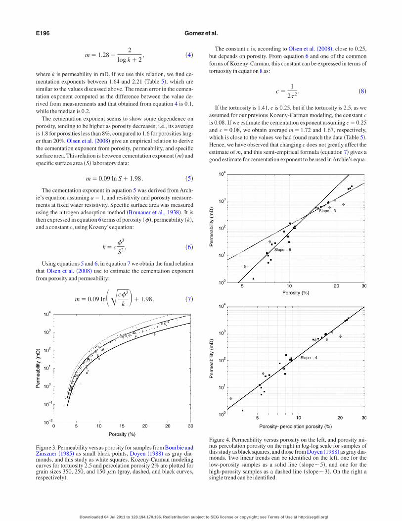
igure 3. Permeability versus porosity for samples from Bourbie andinszner �1985� as small black points, Doyen �1988� as gray dia-onds, and this study as white squares. Kozeny-Carman modeling

urves for tortuosity 2.5 and percolation porosity 2% are plotted forrain sizes 350, 250, and 150 �m �gray, dashed, and black curves,espectively�.


The constant c is, according to Olsen et al. �2008�, close to 0.25,ut depends on porosity. From equation 6 and one of the commonorms of Kozeny-Carman, this constant can be expressed in terms ofortuosity in equation 8 as:

c�1

2� 2 . �8�

If the tortuosity is 1.41, c is 0.25, but if the tortuosity is 2.5, as wessumed for our previous Kozeny-Carman modeling, the constant cs 0.08. If we estimate the cementation exponent assuming c�0.25nd c�0.08, we obtain average m�1.72 and 1.67, respectively,hich is close to the values we had found match the data �Table 5�.ence, we have observed that changing c does not greatly affect the

stimate of m, and this semi-empirical formula �equation 7� gives aood estimate for cementation exponent to be used inArchie’s equa-

Per

mea

bilit

y(m

D)

Porosity (%)

410

310

210

110

010

Slope ~ 5

Slope ~ 3

5 10 20 30

Per

mea

bilit

y(m

D)

Porosity- percolation porosity (%)

410

310

210

110

010

Slope ~ 4

5 10 20 30

igure 4. Permeability versus porosity on the left, and porosity mi-us percolation porosity on the right in log-log scale for samples ofhis study as black squares, and those from Doyen �1988� as gray dia-

onds. Two linear trends can be identified on the left, one for theow-porosity samples as a solid line �slope�5�, and one for theigh-porosity samples as a dashed line �slope�3�. On the right aingle trend can be identified.


ta

Cp

f�deaepvsit�a

Atmmr

fsf�pw7pfat

ttlaArp

w0ad�c2fmmsitt�vifmpAwo

R

a

Fsdfi

F�bat0�g


ion. The mean and the median errors in the cementation exponentre also 0.1 and 0.2.

ementation exponent estimation from mercuryorosimetry

We performed mercury intrusion porosimetry in small drillingragments ��mass�1–1.5 g� of three samples of similar porosity�7%�: A11, A33, and A82, to study the distribution of pore accessiameters. This technique measures the volume of mercury that pen-trates a sample as a function of pressure �Aligizaki, 2006�. Resultsre generally reported using cumulative intrusion curves and differ-ntial pore size distribution plots. Cumulative intrusion curves arelots of the cumulative volume of mercury intruded in the sampleersus the pore throat or pore access diameter. The differential poreize distribution is the differential of the volume of mercury intrudedn the sample versus the pore access diameter. A contact angle be-ween sandstone and mercury of 140° was used for our calculationsMetz and Knofel, 1992; Spearing and Matthews, 1991; Milsch etl., 2008�.

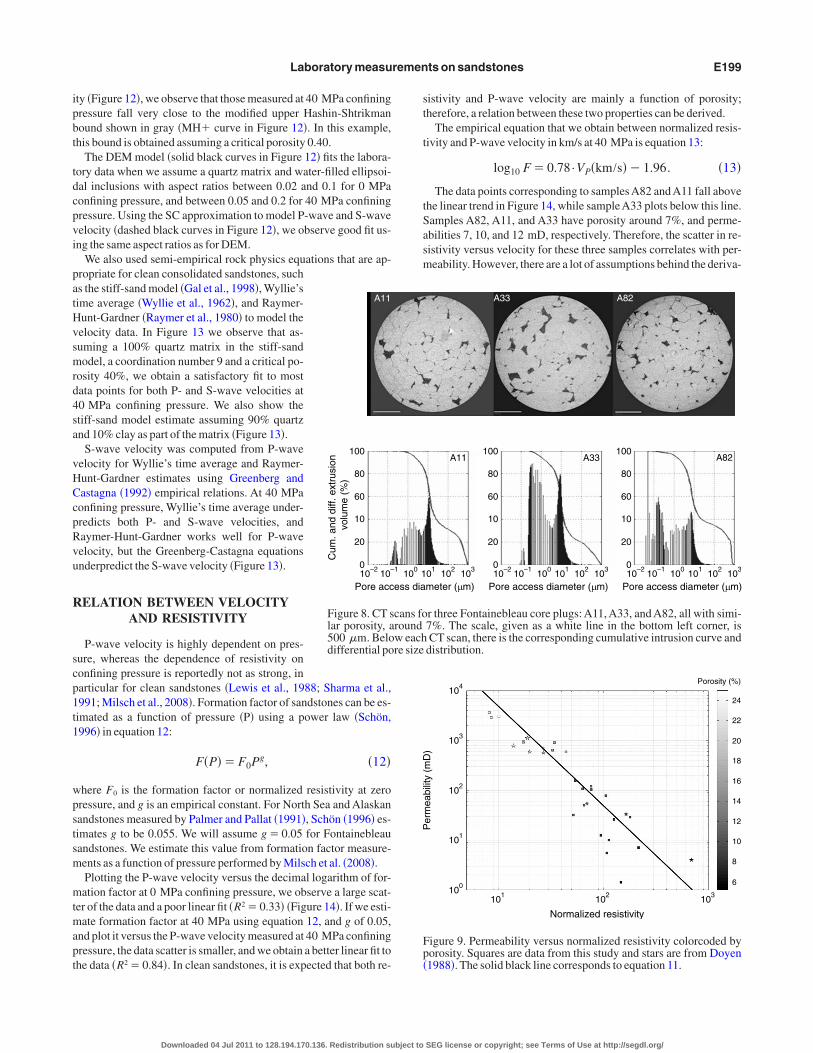
Computed tomography �CT� scans for samples A11, A33, and82 �Figure 8� show that A82 has relatively small macropores, on

he order of 100 microns or less; A11 and A33 have largeracropores, up to 200 microns. This difference in macroporosityay be responsible for the measured larger permeability and lower

esistivity inA11 andA33.Porosity estimates obtained from mercury porosimetry are 8.68%

or A11, 7.18% for A33, and 8.77% for A82. Helium porosity mea-ured for the corresponding core plugs were: 7.33% for A11, 7.18%or A33, and 7.61% for A82. The cumulative intrusion curvesshown as a curve in Figure 8� reveal that samples with the largestorosity, A82 and A11, also have the largest number of pore throatsith diameter larger than 10 �m. The average pore diameters are.0 �m for A11, 3.8 �m for A33, and 3.2 �m for A82. The medianore diameters are 13.0 �m for A11, 8.8 �m for A33, and 9.4 �mor A82. These pore throat distributions are similar as far their meannd median, but they are multimodal �see differential pore size dis-ributions shown as a bar graph in Figure 8�. Comparing the differen-

Cw (S/m)

Co

(S/m

)

1.2

1.0

0.8

0.6

0.4

0.2

0.00 2 4 6 8 10 12 14 16 18 20

y = 0.0813 ×R2 = 0.9903

y = 0.0449 ×R2 = 0.9985

y = 0.011 ×R2 = 0.9987

y = 0.0043 ×R2 = 0.9959

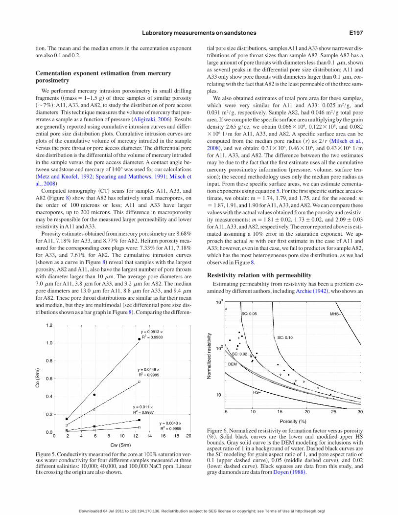
igure 5. Conductivity measured for the core at 100% saturation ver-us water conductivity for four different samples measured at threeifferent salinities: 10,000; 40,000, and 100,000 NaCl ppm. Linearts crossing the origin are also shown.


ial pore size distributions, samplesA11 andA33 show narrower dis-ributions of pore throat sizes than sample A82. Sample A82 has aarge amount of pore throats with diameters less than 0.1 �m, showns several peaks in the differential pore size distribution; A11 and33 only show pore throats with diameters larger than 0.1 �m, cor-

elating with the fact thatA82 is the least permeable of the three sam-les.

We also obtained estimates of total pore area for these samples,hich were very similar for A11 and A33: 0.025 m2 /g, and.031 m2 /g, respectively. Sample A82, had 0.046 m2 /g total porerea. If we compute the specific surface area multiplying by the grainensity 2.65 g /cc, we obtain 0.066�106, 0.122�106, and 0.082106 1 /m for A11, A33, and A82. A specific surface area can be

omputed from the median pore radius �r� as 2 /r �Milsch et al.,008�, and we obtain: 0.31�106, 0.46�106, and 0.43�106 1 /mor A11, A33, and A82. The difference between the two estimatesay be due to the fact that the first estimate uses all the cumulativeercury porosimetry information �pressure, volume, surface ten-

ion�; the second methodology uses only the median pore radius asnput. From these specific surface areas, we can estimate cementa-ion exponents using equation 5. For the first specific surface area es-imate, we obtain: m�1.74, 1.79, and 1.75, and for the second: m

1.87, 1.91, and 1.90 forA11,A33, andA82. We can compare thesealues with the actual values obtained from the porosity and resistiv-ty measurements: m�1.81�0.02, 1.73�0.02, and 2.09�0.03orA11,A33, andA82, respectively. The error reported above is esti-ated assuming a 10% error in the saturation exponent. We ap-

roach the actual m with our first estimate in the case of A11 and33; however, even in that case, we fail to predict m for sampleA82,hich has the most heterogeneous pore size distribution, as we hadbserved in Figure 8.

esistivity relation with permeabilityEstimating permeability from resistivity has been a problem ex-

mined by different authors, including Archie �1942�, who shows an

Porosity (%)

Nor

mal

ized

resi

stiv

ity

5 10 15 20 30

310

210

110

SC: 0.05 MHS+

SC: 0.10

SC: 0.02

DEM

HS–

25

igure 6. Normalized resistivity or formation factor versus porosity%�. Solid black curves are the lower and modified-upper HSounds. Gray solid curve is the DEM modeling for inclusions withspect ratio of 1 in a background of water. Dashed black curves arehe SC modeling for grain aspect ratio of 1, and pore aspect ratio of.1 �upper dashed curve�, 0.05 �middle dashed curve�, and 0.02lower dashed curve�. Black squares are data from this study, andray diamonds are data from Doyen �1988�.


asntpt

w

gti1

w

ml1p

fiba

1v

p

wFwtdt

uc

acptti

ws1ss

TtRer

S

A

A

A

A

A

A

A

B

B

B

B

B

F

G

G

G

G

G

H

H

H

F

FF�

E198 Gomez et al.

verage trend of formation factor versus permeability for sand-tones, but recognizes that the scatter is too large to establish a defi-ite relation between the two properties. Worthington �1997� revisitshis study by Archie and shows how formation factor F decreases asermeability increases according to the following relation in equa-ion 9:

k�� b

F�1/c

. �9�

here b and c are positive empirical constants.Worthington �1997� argues that as water salinity decreases, or

rain size decreases, or the clay content increases, the relation be-ween resistivity and permeability changes and resistivity actuallyncreases as permeability increases in the following form in equation0:

k�gFh. �10�

here g and h are positive empirical constants.Some other relations derived between formation factor and per-eability incorporate other parameters, such as the characteristic

ength of the pore space �Katz and Thompson, 1986; Johnson et al.,986�, the porosity, the specific surface area and the cementation ex-onent �Schwartz et al., 1989�.

If we plot our measured formation factor versus permeability, wend significant scatter, particularly at high resistivity. Still, a trendetween these two variables in the form of equation 9 can be defineds follows in equation 11:

k��702

F�1/0.5

. �11�

The R2 for this trend is 0.92, but the norm of the residuals is32 mD �due to large data scatter at low porosity�; hence, it is notery precise and has to be used with caution �Figure 9�.

VELOCITY RELATION WITH CONFININGPRESSURE AND POROSITY

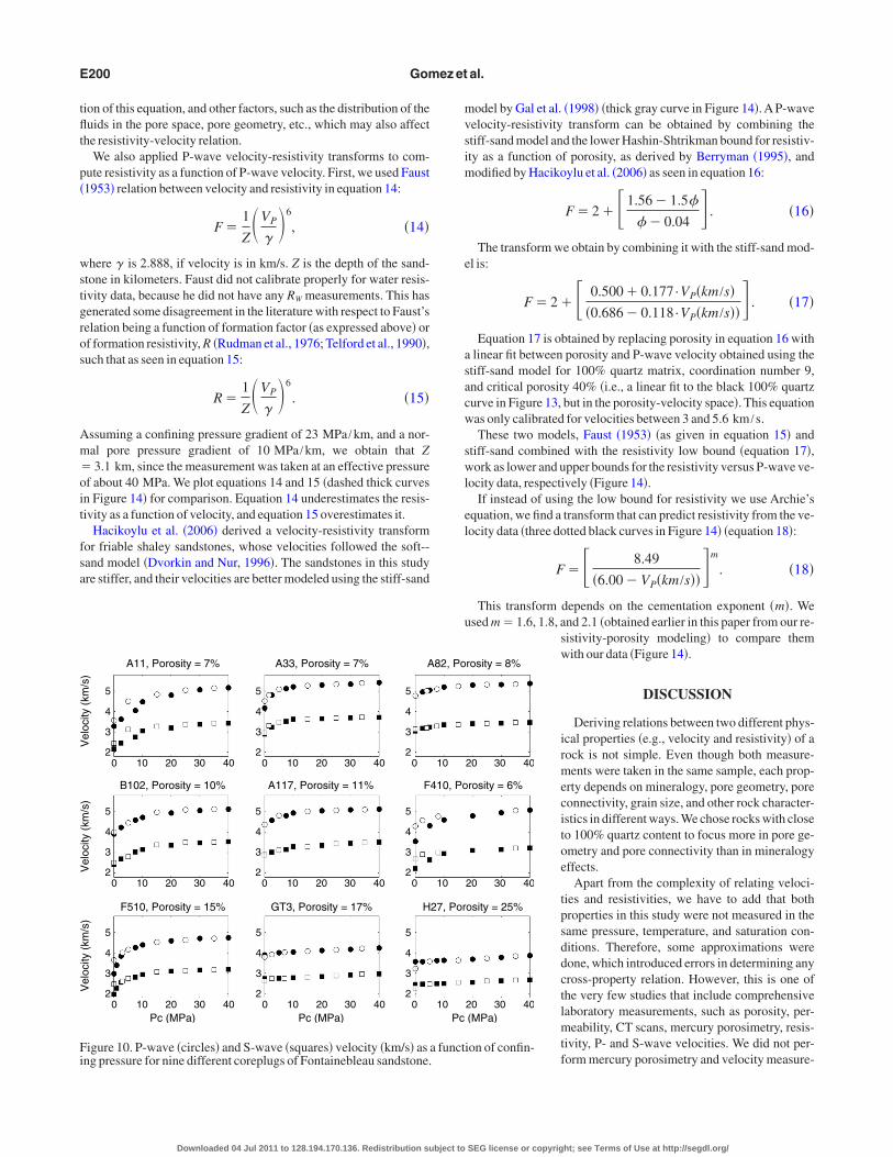
P- and S-wave velocities were measured as functions of confiningressure for 9 samples as shown in Figure 10 �Pwave as circles and S

Porosity (%)

Nor

mal

ized

resi

stiv

ity

310

210

110

5 10 15 20 25 30

2.1

1.8

m = 1.6

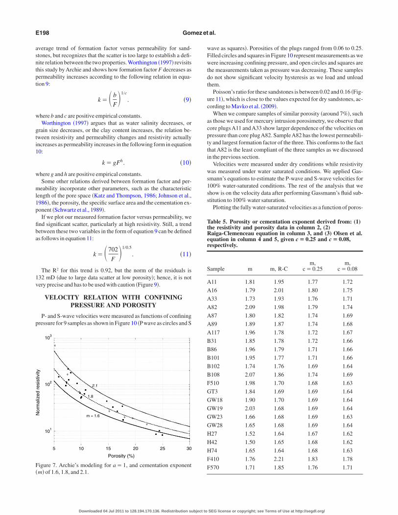
igure 7. Archie’s modeling for a�1, and cementation exponentm� of 1.6, 1.8, and 2.1.


ave as squares�. Porosities of the plugs ranged from 0.06 to 0.25.illed circles and squares in Figure 10 represent measurements as weere increasing confining pressure, and open circles and squares are

he measurements taken as pressure was decreasing. These sampleso not show significant velocity hysteresis as we load and unloadhem.

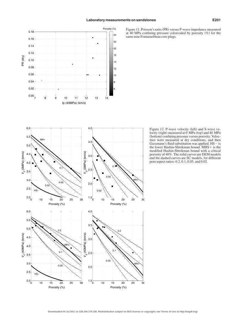
Poisson’s ratio for these sandstones is between 0.02 and 0.16 �Fig-re 11�, which is close to the values expected for dry sandstones, ac-ording to Mavko et al. �2009�.

When we compare samples of similar porosity �around 7%�, suchs those we used for mercury intrusion porosimetry, we observe thatore plugs A11 and A33 show larger dependence of the velocities onressure than core plugA82. SampleA82 has the lowest permeabili-y and largest formation factor of the three. This conforms to the facthat A82 is the least compliant of the three samples as we discussedn the previous section.

Velocities were measured under dry conditions while resistivityas measured under water saturated conditions. We applied Gas-

mann’s equations to estimate the P-wave and S-wave velocities for00% water-saturated conditions. The rest of the analysis that wehow is on the velocity data after performing Gassmann’s fluid sub-titution to 100% water saturation.

Plotting the fully water-saturated velocities as a function of poros-

able 5. Porosity or cementation exponent derived from: (1)he resistivity and porosity data in column 2, (2)aiga-Clemenceau equation in column 3, and (3) Olsen et al.

quation in column 4 and 5, given c�0.25 and c�0.08,espectively.

ample m m, R-Cm,

c�0.25m,

c�0.08

11 1.81 1.95 1.77 1.72

16 1.79 2.01 1.80 1.75

33 1.73 1.93 1.76 1.71

82 2.09 1.98 1.79 1.74

87 1.80 1.82 1.74 1.69

89 1.89 1.87 1.74 1.68

117 1.96 1.78 1.72 1.67

31 1.85 1.78 1.72 1.66

86 1.96 1.79 1.71 1.66

101 1.95 1.77 1.71 1.66

102 1.74 1.76 1.69 1.64

108 2.07 1.86 1.74 1.69

510 1.98 1.70 1.68 1.63

T3 1.84 1.69 1.69 1.64

W18 1.90 1.70 1.69 1.64

W19 2.03 1.68 1.69 1.64

W23 1.66 1.68 1.69 1.63

W28 1.65 1.68 1.69 1.64

27 1.52 1.64 1.67 1.62

42 1.50 1.65 1.68 1.62

74 1.65 1.64 1.68 1.63

410 1.76 2.21 1.83 1.78

570 1.71 1.85 1.76 1.71


ipbt

tdcpvi

patHvsmrd4sa

vHCcpRvu

R

scp1t1

wpstsm

mtmapt

st

t

tSasm

Fp�


ty �Figure 12�, we observe that those measured at 40 MPa confiningressure fall very close to the modified upper Hashin-Shtrikmanound shown in gray �MH� curve in Figure 12�. In this example,his bound is obtained assuming a critical porosity 0.40.

The DEM model �solid black curves in Figure 12� fits the labora-ory data when we assume a quartz matrix and water-filled ellipsoi-al inclusions with aspect ratios between 0.02 and 0.1 for 0 MPaonfining pressure, and between 0.05 and 0.2 for 40 MPa confiningressure. Using the SC approximation to model P-wave and S-waveelocity �dashed black curves in Figure 12�, we observe good fit us-ng the same aspect ratios as for DEM.

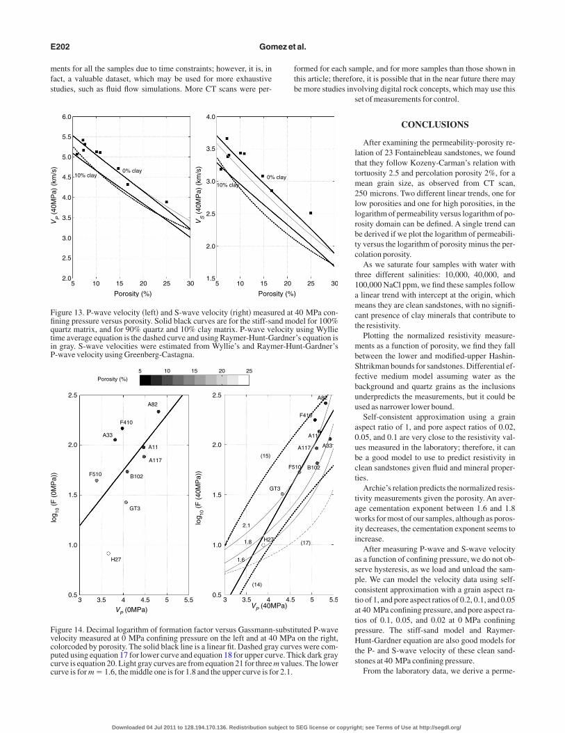
We also used semi-empirical rock physics equations that are ap-ropriate for clean consolidated sandstones, suchs the stiff-sand model �Gal et al., 1998�, Wyllie’sime average �Wyllie et al., 1962�, and Raymer-unt-Gardner �Raymer et al., 1980� to model theelocity data. In Figure 13 we observe that as-uming a 100% quartz matrix in the stiff-sandodel, a coordination number 9 and a critical po-

osity 40%, we obtain a satisfactory fit to mostata points for both P- and S-wave velocities at0 MPa confining pressure. We also show thetiff-sand model estimate assuming 90% quartznd 10% clay as part of the matrix �Figure 13�.

S-wave velocity was computed from P-waveelocity for Wyllie’s time average and Raymer-unt-Gardner estimates using Greenberg andastagna �1992� empirical relations. At 40 MPaonfining pressure, Wyllie’s time average under-redicts both P- and S-wave velocities, andaymer-Hunt-Gardner works well for P-waveelocity, but the Greenberg-Castagna equationsnderpredict the S-wave velocity �Figure 13�.

ELATION BETWEEN VELOCITYAND RESISTIVITY

P-wave velocity is highly dependent on pres-ure, whereas the dependence of resistivity ononfining pressure is reportedly not as strong, inarticular for clean sandstones �Lewis et al., 1988; Sharma et al.,991; Milsch et al., 2008�. Formation factor of sandstones can be es-imated as a function of pressure �P� using a power law �Schön,996� in equation 12:

F�P��F0Pg, �12�

here F0 is the formation factor or normalized resistivity at zeroressure, and g is an empirical constant. For North Sea and Alaskanandstones measured by Palmer and Pallat �1991�, Schön �1996� es-imates g to be 0.055. We will assume g�0.05 for Fontainebleauandstones. We estimate this value from formation factor measure-ents as a function of pressure performed by Milsch et al. �2008�.Plotting the P-wave velocity versus the decimal logarithm of for-ation factor at 0 MPa confining pressure, we observe a large scat-

er of the data and a poor linear fit �R2�0.33� �Figure 14�. If we esti-ate formation factor at 40 MPa using equation 12, and g of 0.05,

nd plot it versus the P-wave velocity measured at 40 MPa confiningressure, the data scatter is smaller, and we obtain a better linear fit tohe data �R2�0.84�. In clean sandstones, it is expected that both re-

A11

Pore acc

Cum

.and

diff.

extr

usio

nvo

lum

e(%

)

100

80

60

10

20

0 –10–210

Figure 8. CT slar porosity, a500 �m. Belodifferential po


istivity and P-wave velocity are mainly a function of porosity;herefore, a relation between these two properties can be derived.

The empirical equation that we obtain between normalized resis-ivity and P-wave velocity in km/s at 40 MPa is equation 13:

log10 F�0.78·VP�km/s��1.96. �13�

The data points corresponding to samples A82 and A11 fall abovehe linear trend in Figure 14, while sample A33 plots below this line.amples A82, A11, and A33 have porosity around 7%, and perme-bilities 7, 10, and 12 mD, respectively. Therefore, the scatter in re-istivity versus velocity for these three samples correlates with per-eability. However, there are a lot of assumptions behind the deriva-

A33 A82

meter (µm) Pore access diameter (µm) Pore access diameter (µm)

31021010

100

80

60

10

20

0 310210110010–110–210

100

80

60

10

20

0 310210110010–110–210

A11 A33 A82

r three Fontainebleau core plugs: A11, A33, and A82, all with simi-7%. The scale, given as a white line in the bottom left corner, isCT scan, there is the corresponding cumulative intrusion curve and

distribution.

Per

mea

bilit

y(m

D)

Normalized resistivity

Porosity (%)

24

22

20

18

16

14

12

10

8

6

410

310

210

110

010 210110 310

igure 9. Permeability versus normalized resistivity colorcoded byorosity. Squares are data from this study and stars are from Doyen1988�. The solid black line corresponds to equation 11.

ess dia10101

cans foroundw eachre size


tflt

p�

wstgros

Am�oit

fsa

mvsim

e

asacw

swl

el

u

Fi

E200 Gomez et al.

ion of this equation, and other factors, such as the distribution of theuids in the pore space, pore geometry, etc., which may also affect

he resistivity-velocity relation.We also applied P-wave velocity-resistivity transforms to com-

ute resistivity as a function of P-wave velocity. First, we used Faust1953� relation between velocity and resistivity in equation 14:

F�1

Z�VP

��6

, �14�

here � is 2.888, if velocity is in km/s. Z is the depth of the sand-tone in kilometers. Faust did not calibrate properly for water resis-ivity data, because he did not have any RW measurements. This hasenerated some disagreement in the literature with respect to Faust’selation being a function of formation factor �as expressed above� orf formation resistivity, R �Rudman et al., 1976; Telford et al., 1990�,uch that as seen in equation 15:

R�1

Z�VP

��6

. �15�

ssuming a confining pressure gradient of 23 MPa /km, and a nor-al pore pressure gradient of 10 MPa /km, we obtain that Z3.1 km, since the measurement was taken at an effective pressure

f about 40 MPa. We plot equations 14 and 15 �dashed thick curvesn Figure 14� for comparison. Equation 14 underestimates the resis-ivity as a function of velocity, and equation 15 overestimates it.

Hacikoylu et al. �2006� derived a velocity-resistivity transformor friable shaley sandstones, whose velocities followed the soft--and model �Dvorkin and Nur, 1996�. The sandstones in this studyre stiffer, and their velocities are better modeled using the stiff-sand

Pc (MPa)Pc (MPa)

Vel

ocity

(km

/s)

Vel

ocity

(km

/s)

Vel

ocity

(km

/s)

F510, Porosity = 15% GT3, Porosity = 17% H

B102, Porosity = 10% A117, Porosity = 11% F

A11, Porosity = 7% A33, Porosity = 7% A

5

4

3

20 10 20 30 40

5

4

3

20 10 20 30 40

5

4

3

20

5

4

3

20 10 20 30 40

5

4

3

20 10 20 30 40

5

4

3

20

5

4

3

20 10 20 30 40

5

4

3

20 10 20 30 40

5

4

3

20

igure 10. P-wave �circles� and S-wave �squares� velocity �km/s� asng pressure for nine different coreplugs of Fontainebleau sandstone.


odel by Gal et al. �1998� �thick gray curve in Figure 14�. A P-waveelocity-resistivity transform can be obtained by combining thetiff-sand model and the lower Hashin-Shtrikman bound for resistiv-ty as a function of porosity, as derived by Berryman �1995�, and

odified by Hacikoylu et al. �2006� as seen in equation 16:

F�2�1.56�1.5�

� �0.04 . �16�

The transform we obtain by combining it with the stiff-sand mod-l is:

F�2� 0.500�0.177·VP�km/s��0.686�0.118·VP�km/s�� . �17�

Equation 17 is obtained by replacing porosity in equation 16 withlinear fit between porosity and P-wave velocity obtained using the

tiff-sand model for 100% quartz matrix, coordination number 9,nd critical porosity 40% �i.e., a linear fit to the black 100% quartzurve in Figure 13, but in the porosity-velocity space�. This equationas only calibrated for velocities between 3 and 5.6 km /s.These two models, Faust �1953� �as given in equation 15� and

tiff-sand combined with the resistivity low bound �equation 17�,ork as lower and upper bounds for the resistivity versus P-wave ve-

ocity data, respectively �Figure 14�.If instead of using the low bound for resistivity we use Archie’s

quation, we find a transform that can predict resistivity from the ve-ocity data �three dotted black curves in Figure 14� �equation 18�:

F� 8.49

�6.00�VP�km/s��m

. �18�

This transform depends on the cementation exponent �m�. Wesed m�1.6, 1.8, and 2.1 �obtained earlier in this paper from our re-

sistivity-porosity modeling� to compare themwith our data �Figure 14�.

DISCUSSION

Deriving relations between two different phys-ical properties �e.g., velocity and resistivity� of arock is not simple. Even though both measure-ments were taken in the same sample, each prop-erty depends on mineralogy, pore geometry, poreconnectivity, grain size, and other rock character-istics in different ways. We chose rocks with closeto 100% quartz content to focus more in pore ge-ometry and pore connectivity than in mineralogyeffects.

Apart from the complexity of relating veloci-ties and resistivities, we have to add that bothproperties in this study were not measured in thesame pressure, temperature, and saturation con-ditions. Therefore, some approximations weredone, which introduced errors in determining anycross-property relation. However, this is one ofthe very few studies that include comprehensivelaboratory measurements, such as porosity, per-meability, CT scans, mercury porosimetry, resis-tivity, P- and S-wave velocities. We did not per-form mercury porosimetry and velocity measure-

(MPa)

osity = 25%

rosity = 6%

rosity = 8%

20 30 40

20 30 40

20 30 40

ion of confin-

Pc

27, Por

410, Po

82, Po

10

10

10

a funct


P
R(d

ry)

Ip (40MPa) (km/s)

Porosity (%)

7 8 9 10 11 12 13 14

0.18

0.16

0.14

0.12

0.10

0.08

0.06

0.04

0.02

0.00

24

22

20

16

14

12

10

8

6

Figure 11. Poisson’s ratio �PR� versus P-wave impedance measuredat 40 MPa confining pressure colorcoded by porosity �%� for thesame nine Fontainebleau core plugs.

Porosity (%) Porosity (%)

V(0

MP

a)(k

m/s

)P

6.0

5.5

5.0

4.5

4.0

3.5

3.0

2.5

2.0

4.0

3.5

3.0

2.5

2.0

1.5

V(0

MP

a)(k

m/s

)S

5 10 15 20 25 30 5 10 15 20 25 30

MH+

0.1

0.050.02

HS–

0.1

0.05

0.02

MH+

Porosity (%) Porosity (%)

V(4

0MP

a)(k

m/s

)P

6.0

5.5

5.0

4.5

4.0

3.5

3.0

2.5

2.0

4.0

3.5

3.0

2.5

2.0

1.5

V(4

0MP

a)(k

m/s

)S

5 10 15 20 25 30 5 10 15 20 25 30

MH+

0.1

0.05

0.2

HS–

0.1

0.05

0.2

MH+

Figure 12. P-wave velocity �left� and S-wave ve-locity �right� measured at 0 MPa �top� and 40 MPa�bottom� confining pressure versus porosity. Veloc-ities were measured at dry conditions, and thenGassmann’s fluid substitution was applied. HS� isthe lower Hashin-Shtrikman bound. MHS� is themodified Hashin-Shtrikman bound with a criticalporosity of 40%. The solid curves are DEM modelsand the dashed curves are SC models, for differentpore aspect ratios: 0.2, 0.1, 0.05, and 0.02.

Downloaded 04 Jul 2011 to 128.194.170.136. Redistribution subject to SEG license or copyright; see Terms of Use at http://segdl.org/

mfs

ftb

FfiqtiP

Fvcpcc

E202 Gomez et al.

ents for all the samples due to time constraints; however, it is, inact, a valuable dataset, which may be used for more exhaustivetudies, such as fluid flow simulations. More CT scans were per-

Porosity (%) Poro

V(4

0MP

a)(k

m/s

)P

6.0

5.5

5.0

4.5

4.0

3.5

3.0

2.5

2.0

4.0

3.5

3.0

2.5

2.0

1.5

V(4

0MP

a)(k

m/s

)S

5 10 15 20 25 30 5 10 15

10% clay0% clay

10% clay0%

igure 13. P-wave velocity �left� and S-wave velocity �right� measuning pressure versus porosity. Solid black curves are for the stiff-sauartz matrix, and for 90% quartz and 10% clay matrix. P-wave veime average equation is the dashed curve and using Raymer-Hunt-Gn gray. S-wave velocities were estimated from Wyllie’s and Raym-wave velocity using Greenberg-Castagna.

V (0MPa)PV (40MP

log

(F(0

MP

a))

10

log

(F(4

0MP

a))

10

2.5

2.0

1.5

1.0

0.53 3.5 4 4.5 5 5.5

2.5

2.0

1.5

1.0

0.53 3.5 4

Porosity (%)

5 10 15 20 25

F410

A82

A33

A117

B102

GT3

H27

F510

A11

(14)

1.6

1.8 H27

G

(15)

2.1

igure 14. Decimal logarithm of formation factor versus Gassmannelocity measured at 0 MPa confining pressure on the left and at 4olorcoded by porosity. The solid black line is a linear fit. Dashed grauted using equation 17 for lower curve and equation 18 for upper cuurve is equation 20. Light gray curves are from equation 21 for threeurve is for m�1.6, the middle one is for 1.8 and the upper curve is f


ormed for each sample, and for more samples than those shown inhis article; therefore, it is possible that in the near future there maye more studies involving digital rock concepts, which may use this

set of measurements for control.

CONCLUSIONS

After examining the permeability-porosity re-lation of 23 Fontainebleau sandstones, we foundthat they follow Kozeny-Carman’s relation withtortuosity 2.5 and percolation porosity 2%, for amean grain size, as observed from CT scan,250 microns. Two different linear trends, one forlow porosities and one for high porosities, in thelogarithm of permeability versus logarithm of po-rosity domain can be defined. A single trend canbe derived if we plot the logarithm of permeabili-ty versus the logarithm of porosity minus the per-colation porosity.

As we saturate four samples with water withthree different salinities: 10,000, 40,000, and100,000 NaCl ppm, we find these samples followa linear trend with intercept at the origin, whichmeans they are clean sandstones, with no signifi-cant presence of clay minerals that contribute tothe resistivity.

Plotting the normalized resistivity measure-ments as a function of porosity, we find they fallbetween the lower and modified-upper Hashin-Shtrikman bounds for sandstones. Differential ef-fective medium model assuming water as thebackground and quartz grains as the inclusionsunderpredicts the measurements, but it could beused as narrower lower bound.

Self-consistent approximation using a grainaspect ratio of 1, and pore aspect ratios of 0.02,0.05, and 0.1 are very close to the resistivity val-ues measured in the laboratory; therefore, it canbe a good model to use to predict resistivity inclean sandstones given fluid and mineral proper-ties.

Archie’s relation predicts the normalized resis-tivity measurements given the porosity. An aver-age cementation exponent between 1.6 and 1.8works for most of our samples, although as poros-ity decreases, the cementation exponent seems toincrease.

After measuring P-wave and S-wave velocityas a function of confining pressure, we do not ob-serve hysteresis, as we load and unload the sam-ple. We can model the velocity data using self-consistent approximation with a grain aspect ra-tio of 1, and pore aspect ratios of 0.2, 0.1, and 0.05at 40 MPa confining pressure, and pore aspect ra-tios of 0.1, 0.05, and 0.02 at 0 MPa confiningpressure. The stiff-sand model and Raymer-Hunt-Gardner equation are also good models forthe P- and S-wave velocity of these clean sand-stones at 40 MPa confining pressure.

From the laboratory data, we derive a perme-

25 30

40 MPa con-del for 100%using Wyllie’s equation isnt-Gardner’s

5 5.5

(17)

10 B102

A117 A33

A11

F410

A82

tuted P-waveon the right,

es were com-ick dark grayes. The lower

sity (%)

20

clay

red atnd molocityardnerer-Hu

Pa)4.5

T3

F5

-substi0 MPay curvrve. Thm valuor 2.1.


antc

ccawAe

mcd

ppTtd

A

A

B

B

B

B

C

C

D

D

D

D

F

G

G

G

H

H

J

J

J

K

K

K

K

L

L

M

M

M

—M

—

M

M

M

N

O

O

P

P

P

—

R

R


bility versus formation factor relation, which has a high R2, but theorm of the residuals is also high. We conclude that overall forma-ion factor is not a good predictor of permeability, even in the case oflean sandstones.

We conclude that both velocity and resistivity in clean sandstonesan be modeled using self-consistent approximation. In addition, wean find a linear fit between the P-wave velocity and the decimal log-rithm of the normalized resistivity, with deviations that correlateith differences in permeability. Combining the stiff sand model andrchie for cementation exponents between 1.6 and 2.1, we can mod-

l resistivity as a function of P-wave velocity.In the future, it would be desirable to perform velocity measure-ents for more samples to have a more complete dataset, and also to

arry out some of the resistivity measurements under pressure in or-er to calibrate our own pressure-resistivity relation.

ACKNOWLEDGMENTS

I would like to acknowledge SRB sponsors for their financial sup-ort. Thanks to Bernard Zinsner at the Institut Français du Pétrole forroviding the samples. Thanks to InGrain for providing CT scans.hanks to Stéphanie Vialle, Stanford University, for her help with

he mercury porosimetry. I would also like to thank Barry Kirken-all, Stanford University, for his help with the resistivity equipment.

REFERENCES

ligizaki, K., 2006, Pore structure of cement-based materials: testing, inter-pretation and requirements: Taylor & Francis.

rchie, G. E., 1942, The electrical resistivity log as an aid in determiningsome reservoir characteristics: Transactions of the American Institute ofMining, Metallurgical, and Petroleum Engineers, 146, 54–62.

erryman, J., 1995, Mixture of Rock Properties, in T. J. Ahrens, ed., Hand-book of physical constants:American Geophysical Union Reference Shelf3, 205–228.

ourbie, T., and B. Zinszner, 1985, Hydraulic and acoustic properties as afunction of porosity in Fontainebleau sandstone: Journal of GeophysicalResearch, 90, B13, 11524–11532, doi: 10.1029/JB090iB13p11524.

ruggeman, D. A. G., 1935, Berechnung verschiedener physikalischer Kon-stanten von heterogenen Substanzen: Annalen der Physik �Leipzig�, 24,no. 7, 636–664, doi: 10.1002/andp.19354160705.Bruggeman.

runauer, S., P. Emmett, and E. Teller, 1938, Adsorption of gases in multi-molecular layers: Journal of the American Chemical Society, 60, no. 2,309–319, doi: 10.1021/ja01269a023.

arman, P. C., 1961, L’écoulement des gaz à travers les milieux poreux: Bib-liothèque des Sciences et des Techniques nucléaires, P.U.F., 52.

arrara, E., A. Mazzacca, R. Pece, N. Roberti, and T. Vanorio, 1999, Evalua-tion of porosity and saturation degree by laboratory joint measurements ofvelocity and resistivity: Pure and Applied Geophysics, 154, no. 2,211–255, doi: 10.1007/s000240050228.

omenico, S. N., 1976, Effect of brine-gas mixture on velocity in an uncon-solidated sand reservoir: Geophysics, 41, 882–894, doi: 10.1190/1.1440670.

oyen, P. M., 1988, Permeability, conductivity and pore geometry of sand-stones: Journal of Geophysical Research, 93, B7, 7729–7740, doi:10.1029/JB093iB07p07729.

urand, C., 2003, Improvement of fluid distribution description duringfloods by combined use of X-ray CT scan and continuous local resistivitymeasurements: Symposium of the Society of CoreAnalysts.

vorkin, J., and A. Nur, 1996, Elasticity of high-porosity sandstones: Theoryfor two North Sea datasets: Geophysics, 61, 1363–1370, , doi: 10.1190/1.1444059.

aust, L. Y., 1953, A velocity function including lithologic variation: Geo-physics, 18, 271–288, doi: 10.1190/1.1437869.

al, D., J. Dvorkin, and A. Nur, 1998, A physical model for porosity reduc-tion in sandstones: Geophysics, 63, 454–459, doi: 10.1190/1.1444346.

assmann, F., 1951, Elasticity of porous media: Uber die elastizitat porosermedien: Vierteljahrsschrift der Naturforschenden Gesselschaft in Zurich,96, 1–23.

reenberg, M. L., and J. P. Castagna, 1992, Shear-wave velocity estimationin porous rocks; theoretical formulation, preliminary verification and ap-


plications: Geophysical Prospecting, 40, no. 2, 195–209, doi: 10.1111/j.1365-2478.1992.tb00371.x.

acikoylu, P., J. Dvorkin, and G. Mavko, 2006, Resistivity-velocity trans-forms revisited: The Leading Edge, 25, 1006–1009, doi: 10.1190/1.2335159.

ausenblas, M., 1995, Stress dependence of the cementation exponent: Soci-ety of CoreAnalysts, 9518.

ackson, P. D., D. T. Smith, and P. N. Stanford, 1978, Resistivity-porosity-particle shape relationships for marine sands: Geophysics, 43, 1250–1276,doi: 10.1190/1.1440891.

acquin, C. G., 1964, Correlation entre la permeabilite et les characteris-tiques geometriques du gres de Fontainebleau: Revue de l’InstitutFrançais du Pétrole, 19, 921–937.

ohnson, D., T. Plona, and H. Kojima, 1986, Probing Porous Media with 1stSound, 2nd Sound, 4th Sound and 3rd Sound: Physics and chemistry of po-rous media-II, in J. Banavar, J. Koplik, and K. Winkler, eds., Proceedingsof the Second International Symposium on the Physics and Chemistry ofPorous Media, 154, 243–277.

atz, A. J., and A. H. Thompson, 1986, Quantitative prediction of permeabil-ity in porous rock: Physical Review B, 34, no. 11, 8179–8181, doi:10.1103/PhysRevB.34.8179.PubMed.

nackstedt, M., C. Arns, A. Sheppard, T. Senden, R. Sok, Y. Cinar, A.Olafuyi, W. Pinczewski, G. Padhy, and M. Ioannidis, 2007, Pore scaleanalysis of electrical resistivity in complex core material: Symposium ofthe Society of CoreAnalysts.

night, R., 1991, Hysteresis in the electrical resistivity of partially saturatedsandstones: Geophysics, 56, 2139–2147, doi: 10.1190/1.1443028.

night, R., and A. Endres, 2005, An Introduction to rock physics principlesfor near-surface geophysics, in D. Butler, ed., Near-Surface Geophysics:SEG Investigations in Geophysics 13, 31–70.

andauer, R., 1952, The electrical resistance of binary metallic mixtures:Journal ofApplied Physics, 23, no. 7, 779–784, doi: 10.1063/1.1702301.

ewis, M., M. Sharma, and H. Dunlap, 1988, Techniques for measuring theelectrical properties of sandstone core: Society of Petroleum EngineersAnnual Technical Conference, 697–703.avko, G., 1980, Velocity and attenuation in partially molten rocks: Journalof Geophysical Research, 85, B10, 5173–5189, doi: 10.1029/JB085iB10p05173.avko, G., and T. Mukerji, 1995, Seismic pore space compressibility andGassmann’s relation: Geophysics, 60, 1743–1749, doi: 10.1190/1.1443907.avko, G., T. Mukerji, and J. Dvorkin, 1998, The rock physics handbook:Cambridge University Press.—–, 2009, The rock physics handbook: Cambridge University Press.avko, G., and A. Nur, 1978, The effect of nonelliptical cracks on the com-pressibility of rocks: Journal of Geophysical Research, 83, B9,4459–4468, doi: 10.1029/JB083iB09p04459.—–, 1997, The effect of a percolation threshold in the Kozeny-Carman re-lation: Geophysics, 62, 1480–1482, doi: 10.1190/1.1444251.etz, F., and D. Knofel, 1992, Systematic mercury porosimetry investiga-tions on sandstones: Materials and Structures, 25, no. 3, 127–136, doi:10.1007/BF02472425.ilsch, H., G. Blocher, and S. Engelmann, 2008, The relationship betweenhydraulic and electrical transport properties in sandstones: An experimen-tal evaluation of several scaling models: Earth and Planetary Science Let-ters, 275, no. 3–4, 355–363, doi: 10.1016/j.epsl.2008.08.031.urphy, W. F. III, 1984, Acoustic measures of partial gas saturation in tightsandstones: Journal of Geophysical Research, 89, B13, 11549–11559, doi:10.1029/JB089iB13p11549.

ur, A., and G. Simmons, 1969, The effect of saturation on velocity in lowporosity rocks: Earth and Planetary Science Letters, 7, no. 2, 183–193, doi:10.1016/0012-821X�69�90035-1.

’Connell, R., and B. Budiansky, 1974, Seismic velocities in dry and saturat-ed cracked solids: Journal of Geophysical Research, 79, no. 35,5412–5426, doi: 10.1029/JB079i035p05412.

lsen, C., T. Hongdul, and I. Lykke Fabricius, 2008, Prediction of Archie’scementation factor from porosity and permeability through specific sur-face: Geophysics, 73, no. 2, E81–E87, doi: 10.1190/1.2837303.

almer, T., and N. Pallat, 1991, The effect of overburden pressure on forma-tion factor for shaly sands, Transactions of 14th European Formation Eval-uation Symposium, paper M.

arkhomenko, E. I., 1967, Electrical properties of rocks: Monographs inGeosciences, Plenum Press.

olak, L., and M. Rapoport, 1956, On the relation between electrical andelastic properties in sedimentary rocks: Prikl Geofiz, v. 15.—–, 1961, On the relation of the velocity of elastic waves to some physicalproperties of sedimentary rocks: Prikl Geofiz, v. 29.

aiga-Clemenceau, J., 1977, The cementation exponent in the formation fac-tor — porosity relation: The effect of permeability: Proceedings of the So-ciety and Petrophysicists and Well Logging Analysts 18th Annual Meet-ing, paper R.

ansom, R., 1984, Acontribution towards a better understanding of the mod-


R

R

R

S

S

S

S

T

T

W

W

W

W

W

W

W

—

—

E204 Gomez et al.

ifiedArchie formation resistivity factor relationship: The LogAnalyst, 25,no. 2, 7–12.

aymer, D. S., E. R. Hunt, and J. S. Gardner, 1980, An improved sonic transittime-to-porosity transform, Proceedings of the Society and Petrophysi-cists and Well LoggingAnalysts 21stAnnual Meeting, paper P.

evil, A., and P. Glover, 1997, Theory of ionic-surface electrical conductionin porous media: Physical Review B: Condensed Matter and MaterialsPhysics, 55, no. 3, 1757–1773, doi: 10.1103/PhysRevB.55.1757.

udman, A., J. Whaley, R. Blakely, and M. Biggs, 1976, Transformation ofresistivity to pseudovelocity logs: AAPG Bulletin, 60, 879–882.

chön, J. H., 1996, Physical properties of rocks: Fundamentals and Princi-ples of Petrophysics: Handbook of Geophysical Exploration. Section I,Seismic Exploration: v. 18.

chwartz, L., P. Sen, and D. Johnson, 1989, Influence of rough surface onelectrolytic conduction in porous media: Physical Review B: CondensedMatter and Materials Physics, 40, no. 4, 2450–2458, doi: 10.1103/Phys-RevB.40.2450.

harma, M., A. Garrouch, and H. Dunlap, 1991, Effects of wettability, poregeometry, and stress on electrical conduction in fluid-saturated rocks: TheLogAnalyst, 32, 511–526.

pearing, M., and G. P. Matthews, 1991, Modeling Characteristic Propertiesof Sandstones: Transport in Porous Media, 6, no. 1, 71–90, doi: 10.1007/BF00136822.

elford, W., L. Geldart, and R. Sheriff, 1990, Applied geophysics: Cam-bridge University Press.

homas, E. C., 2007, Clay minerals and their effect upon the electrical be-


havior of shaly sands: Class notes at Denver Well Logging Society.axman, M., and L. Smits, 1968, Electrical conductivities in oil-bearingshaly sands: SPE Journal, 243, 107–122.axman, M., and E. C. Thomas, 1974, Electrical conductivities in shalysands: Journal of Petroleum Technology, 26, 213–225.empe, W., 2000, Predicting flow properties using geophysical data improv-ing aquifer characterization: Ph.D. dissertation, Stanford University.orthington, P., 1993, The uses and abuses of the Archie equations;, 1, Theformation factor-porosity relationship: Journal of Applied Geophysics,30, no. 3, 215–228, doi: 10.1016/0926-9851�93�90028-W.orthington, P., 1997, Petrophysical estimation of permeability as a functionof scale: Developments in Petrophysics, in M. A. Lovell, and P. K. Harvey,eds., Geological Society Special Publications, 122, 159–168.yllie, M., and A. Gregory, 1953, Formation factors of unconsolidated po-rous media: Influence of particle shape and effect of cementation: Transac-tions of the American Institute of Mining, Metallurgical, and PetroleumEngineers, 198, 103–110.yllie, M., A. Gregory, and G. Gardner, 1956, Elastic wave velocities in het-erogeneous and porous media: Geophysics, 21, 41–70, doi: 10.1190/1.1438217.—–, 1958, An experimental investigation of factors affecting elastic wavevelocities in porous media: Geophysics, 23, 459–493, doi: 10.1190/1.1438493.—–, 1962, Studies of elastic wave attenuation in porous media: Geophys-ics, 27, 569–589, doi: 10.1190/1.1439063.


laboratory measurements of porosity, permeability ... · pdf filelaboratory measurements of...

Documents