labor supply in rbc models + calibration - forsiden ... supply in rbc models + calibration lecture...

Labor supply in RBC models + calibrationLecture 12, ECON 4310

Tord Krogh

October 8, 2012

Tord Krogh () ECON 4310 October 8, 2012 1 / 52

Summary from last lecture

Last lecture (#11) we went through

What a solution is for our basic model

How to linearize the deterministic model

How to linearize the stochastic model


Summary from last lecture II

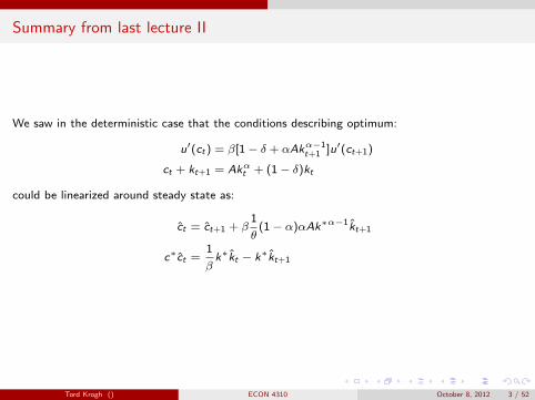
We saw in the deterministic case that the conditions describing optimum:

u′(ct ) = β[1− δ + αAkα−1t+1 ]u′(ct+1)

ct + kt+1 = Akαt + (1− δ)kt

could be linearized around steady state as:

ct = ct+1 + β1

θ(1− α)αAk∗α−1kt+1

c∗ct =1

βk∗kt − k∗kt+1


Summary from last lecture III

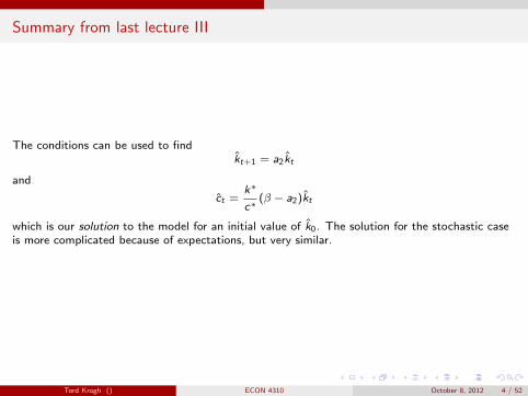
The conditions can be used to findkt+1 = a2kt

and

ct =k∗

c∗(β − a2)kt

which is our solution to the model for an initial value of k0. The solution for the stochastic caseis more complicated because of expectations, but very similar.


Summary from last lecture IV

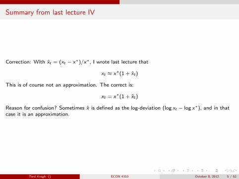
Correction: With xt = (xt − x∗)/x∗, I wrote last lecture that

xt ≈ x∗(1 + xt )

This is of course not an approximation. The correct is:

xt = x∗(1 + xt )

Reason for confusion? Sometimes x is defined as the log-deviation (log xt − log x∗), and in thatcase it is an approximation.


Today’s lecture

Introducing labor supply in the basic modelThe intratemporal optimality conditionFrisch elasticity and IES for labor supply

Labor lotteries

The concept of calibration


Labor supply

Labor supply in the basic model

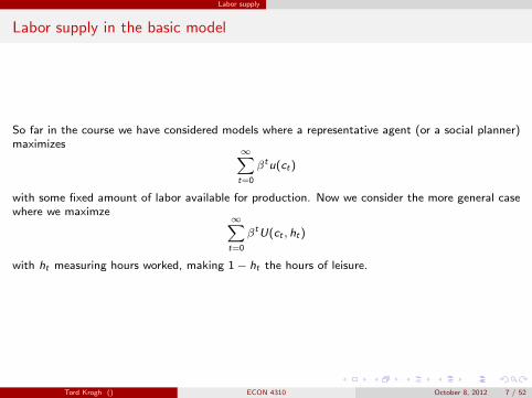
So far in the course we have considered models where a representative agent (or a social planner)maximizes

∞∑t=0

βt u(ct )

with some fixed amount of labor available for production. Now we consider the more general casewhere we maximze

∞∑t=0

βt U(ct , ht )

with ht measuring hours worked, making 1− ht the hours of leisure.


Labor supply

Labor supply in the basic model II

In RBC models we will see that the labor supply response to changes in wages (driven byproductivity shocks) is an important propagation mechanism.


Labor supply

Labor supply in the basic model III

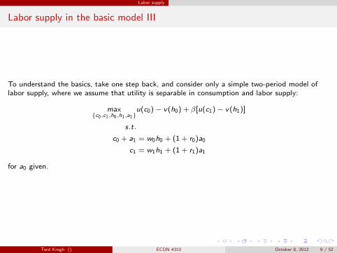
To understand the basics, take one step back, and consider only a simple two-period model oflabor supply, where we assume that utility is separable in consumption and labor supply:

max{c0,c1,h0,h1,a1}

u(c0)− v(h0) + β[u(c1)− v(h1)]

s.t.

c0 + a1 = w0h0 + (1 + r0)a0

c1 = w1h1 + (1 + r1)a1

for a0 given.


Labor supply

Labor supply in the basic model IV

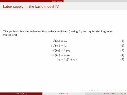
This problem has the following first order conditions (letting λ0 and λ1 be the Lagrangemultipliers)

u′(c0) = λ0 (1)

βu′(c1) = λ1 (2)

v ′(h0) = λ0w0 (3)

βv ′(h1) = λ1w1 (4)

λ0 = λ1(1 + r1) (5)


Labor supply

Labor supply in the basic model V

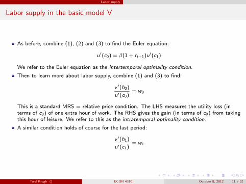
As before, combine (1), (2) and (3) to find the Euler equation:

u′(c0) = β(1 + rt+1)u′(c1)

We refer to the Euler equation as the intertemporal optimality condition.

Then to learn more about labor supply, combine (1) and (3) to find:

v ′(h0)

u′(c0)= w0

This is a standard MRS = relative price condition. The LHS measures the utility loss (interms of c0) of one extra hour of work. The RHS gives the gain (in terms of c0) from takingthis hour of leisure. We refer to this as the intratemporal optimality condition.

A similar condition holds of course for the last period:

v ′(h1)

u′(c1)= w1


Labor supply

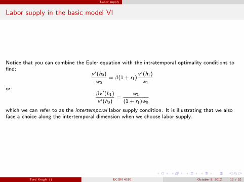
Labor supply in the basic model VI

Notice that you can combine the Euler equation with the intratemporal optimality conditions tofind:

v ′(h0)

w0= β(1 + r1)

v ′(h1)

w1

or:βv ′(h1)

v ′(h0)=

w1

(1 + r1)w0

which we can refer to as the intertemporal labor supply condition. It is illustrating that we alsoface a choice along the intertemporal dimension when we choose labor supply.


Labor supply

Labor supply in the basic model VII

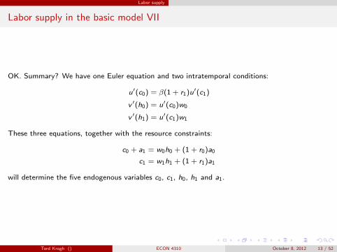
OK. Summary? We have one Euler equation and two intratemporal conditions:

u′(c0) = β(1 + r1)u′(c1)

v ′(h0) = u′(c0)w0

v ′(h1) = u′(c1)w1

These three equations, together with the resource constraints:

c0 + a1 = w0h0 + (1 + r0)a0

c1 = w1h1 + (1 + r1)a1

will determine the five endogenous variables c0, c1, h0, h1 and a1.


Labor supply

Labor supply in the basic model VII

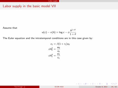
Assume that

u(c)− v(h) = log c − φh1+θ

1 + θ

The Euler equation and the intratemporal conditions are in this case given by:

c1 = β(1 + r1)c0

φhθ0 =w0

c0

φhθ1 =w1

c1


Labor supply

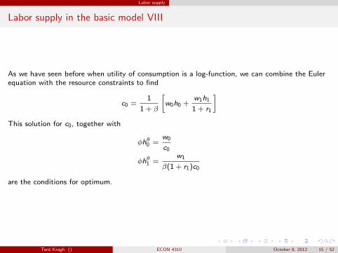
Labor supply in the basic model VIII

As we have seen before when utility of consumption is a log-function, we can combine the Eulerequation with the resource constraints to find

c0 =1

1 + β

[w0h0 +

w1h1

1 + r1

]This solution for c0, together with

φhθ0 =w0

c0

φhθ1 =w1

β(1 + r1)c0

are the conditions for optimum.


Labor supply

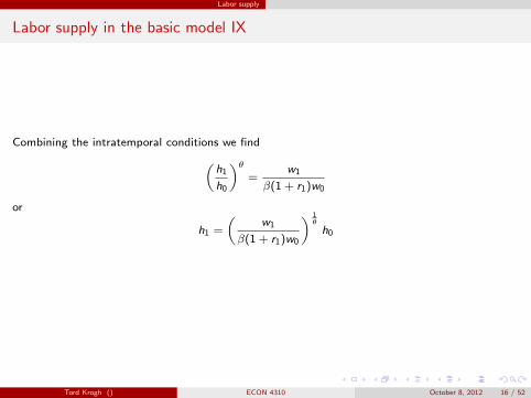
Labor supply in the basic model IX

Combining the intratemporal conditions we find(h1

h0

)θ=

w1

β(1 + r1)w0

or

h1 =

(w1

β(1 + r1)w0

) 1θ

h0


Labor supply

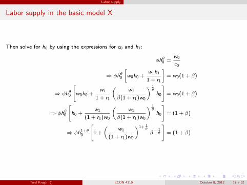
Labor supply in the basic model X

Then solve for h0 by using the expressions for c0 and h1:

φhθ0 =w0

c0

⇒ φhθ0

[w0h0 +

w1h1

1 + r1

]= w0(1 + β)

⇒ φhθ0

[w0h0 +

w1

1 + r1

(w1

β(1 + r1)w0

) 1θ

h0

]= w0(1 + β)

⇒ φhθ0

[h0 +

w1

(1 + r1)w0

(w1

β(1 + r1)w0

) 1θ

h0

]= (1 + β)

⇒ φh1+θ0

[1 +

(w1

(1 + r1)w0

)1+ 1θ

β−1θ

]= (1 + β)


Labor supply

Labor supply in the basic model XI

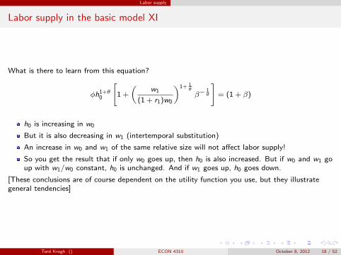
What is there to learn from this equation?

φh1+θ0

[1 +

(w1

(1 + r1)w0

)1+ 1θ

β−1θ

]= (1 + β)

h0 is increasing in w0

But it is also decreasing in w1 (intertemporal substitution)

An increase in w0 and w1 of the same relative size will not affect labor supply!

So you get the result that if only w0 goes up, then h0 is also increased. But if w0 and w1 goup with w1/w0 constant, h0 is unchanged. And if w1 goes up, h0 goes down.

[These conclusions are of course dependent on the utility function you use, but they illustrategeneral tendencies]


Elasticities

Two important elasticities

There are two important elasticities we need to care about:

1 Frisch elasticity: The elasticity of labor supply with respect to the wage, keeping marginalutility of wealth constant. Measures the substitution effect

2 Intertemporal elasticity of substitution (IES) for labor supply: The elasticity of relativelabor supply across periods with respect to the present value of wage growth


Elasticities

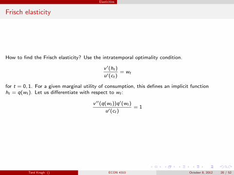
Frisch elasticity

How to find the Frisch elasticity? Use the intratemporal optimality condition.

v ′(ht )

u′(ct )= wt

for t = 0, 1. For a given marginal utility of consumption, this defines an implicit functionht = q(wt ). Let us differentiate with respect to wt :

v ′′(q(wt ))q′(wt )

u′(ct )= 1


Elasticities

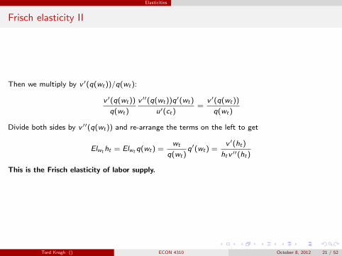
Frisch elasticity II

Then we multiply by v ′(q(wt ))/q(wt ):

v ′(q(wt ))

q(wt )

v ′′(q(wt ))q′(wt )

u′(ct )=

v ′(q(wt ))

q(wt )

Divide both sides by v ′′(q(wt )) and re-arrange the terms on the left to get

Elwt ht = Elwt q(wt ) =wt

q(wt )q′(wt ) =

v ′(ht )

ht v ′′(ht )

This is the Frisch elasticity of labor supply.


Elasticities

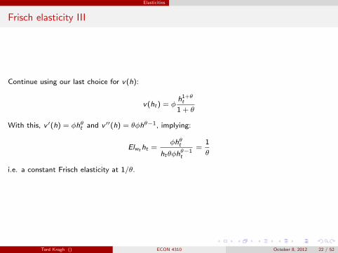
Frisch elasticity III

Continue using our last choice for v(h):

v(ht ) = φh1+θ

t

1 + θ

With this, v ′(h) = φhθt and v ′′(h) = θφhθ−1, implying:

Elwt ht =φhθt

htθφhθ−1t

=1

θ

i.e. a constant Frisch elasticity at 1/θ.


Elasticities

IES for labor supply

What about the IES for labor supply? Keep the particular choice of v(h). To find this elasticity,we use the intertemporal optimality condition for labor:

βv ′(h1)

v ′(h0)=

w1

(1 + r1)w0

which now becomes

β

(h1

h0

)θ=

w1

(1 + r1)w0= W0

where W1 denotes the present value of wage growth.


Elasticities

IES for labor supply II

The IES for labor supply is the elasticity of h1/h0 with respect to W0. To find it, we can eitherfind derivatives etc. like for the Frisch case, or simply use that:

Elx y =d log y

d log x

Taking logs of the intertemporal optimality condition for labor we get:

log β + θ log(h1

h0) = log W0

Hence:

ElW0

h1

h0=

1

θ

In this case the IES for labor supply equals the Frisch elasticity.


Elasticities

Using the elasticities

The higher the Frisch elasticity, the more willing are you to work if the wage increases

The higher the IES for labor supply, the more willing are you to shift the path of labor supplyin response to temporary changes in the wage


Elasticities

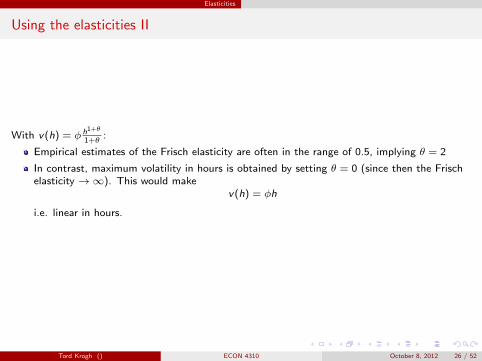
Using the elasticities II

With v(h) = φ h1+θ

1+θ:

Empirical estimates of the Frisch elasticity are often in the range of 0.5, implying θ = 2

In contrast, maximum volatility in hours is obtained by setting θ = 0 (since then the Frischelasticity →∞). This would make

v(h) = φh

i.e. linear in hours.


Elasticities

Using the elasticities III

Since we want to choose values for our structural parameters that are consistent with microevidence, we should also set θ close to 2 in an RBC model.

But values of θ around 2 are often producing too little volatility in labor supply in RBCmodels!

To get more volatile labor supply, one would rather be somewhere closer to θ = 0, in whichcase v(h) is linear in h and we get maximium volatility.

This is a problem

But we know that (e.g. as shown in Kydland and Prescott, 1990) fluctuations in labor supplyseems to be driven primarily by changes in the extensive margin – not so much by the intensive.Can we change our model to account for this?


Elasticities

Labor lotteries

This is the motivation for models of indivisible labor combined with labor lotteries (see Hansen(1984) and Rogerson (1988)).

In the simple model the agent could choose h to be anywhere between zero and one

With indivisible labor, we will require h = {0, 1}, i.e. working becomes a ‘yes/no’ choice

Labor lotteries (Rogerson, 1988) offers an elegant way of introducing this mechanism


Elasticities

Labor lotteries II

Consider the following setting:

There exists a continuum of households on the unit interval, each with a utility function∑∞t=0 β

t [u(ct )− v(ht )]

Hours worked must by each agent is either 0 or 1

All agents agree to join in a ‘labor lottery’: With probability ξt they will have to work, andwith probability 1− ξt they will be unemployed. But no matter if they work or not, all willrecieve the same income (and therefore consumption).

ξt is then chosen by the group or a social planner to maximize welfare

With a continuum of agents, ξt can be interpreted as the share of agents that must work


Elasticities

Labor lotteries III

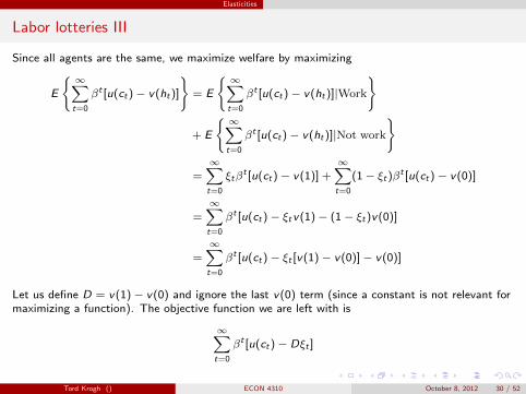
Since all agents are the same, we maximize welfare by maximizing

E

{ ∞∑t=0

βt [u(ct )− v(ht )]

}= E

{ ∞∑t=0

βt [u(ct )− v(ht )]|Work

}

+ E

{ ∞∑t=0

βt [u(ct )− v(ht )]|Not work

}

=∞∑

t=0

ξtβt [u(ct )− v(1)] +

∞∑t=0

(1− ξt )βt [u(ct )− v(0)]

=∞∑

t=0

βt [u(ct )− ξt v(1)− (1− ξt )v(0)]

=∞∑

t=0

βt [u(ct )− ξt [v(1)− v(0)]− v(0)]

Let us define D = v(1)− v(0) and ignore the last v(0) term (since a constant is not relevant formaximizing a function). The objective function we are left with is

∞∑t=0

βt [u(ct )− Dξt ]


Elasticities

Labor lotteries IV

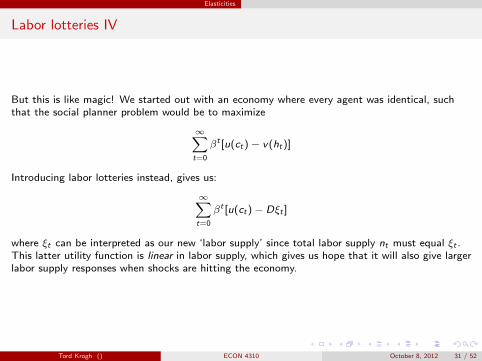
But this is like magic! We started out with an economy where every agent was identical, suchthat the social planner problem would be to maximize

∞∑t=0

βt [u(ct )− v(ht )]

Introducing labor lotteries instead, gives us:

∞∑t=0

βt [u(ct )− Dξt ]

where ξt can be interpreted as our new ‘labor supply’ since total labor supply nt must equal ξt .This latter utility function is linear in labor supply, which gives us hope that it will also give largerlabor supply responses when shocks are hitting the economy.


Elasticities

Labor lotteries V

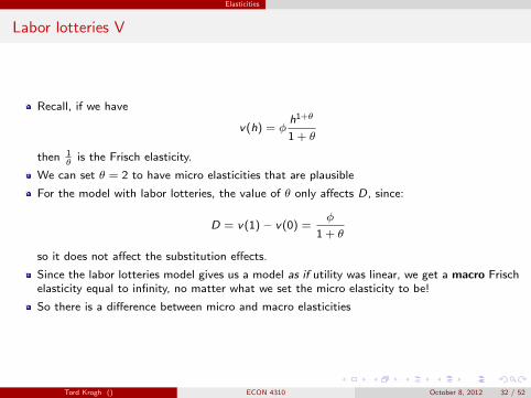
Recall, if we have

v(h) = φh1+θ

1 + θ

then 1θ

is the Frisch elasticity.

We can set θ = 2 to have micro elasticities that are plausible

For the model with labor lotteries, the value of θ only affects D, since:

D = v(1)− v(0) =φ

1 + θ

so it does not affect the substitution effects.

Since the labor lotteries model gives us a model as if utility was linear, we get a macro Frischelasticity equal to infinity, no matter what we set the micro elasticity to be!

So there is a difference between micro and macro elasticities


Elasticities

Labor lotteries VI

Intuition for the possible difference between micro and macro elasticities:

For the micro elasticity, we look at the effect on hours worked from a marginal change in thewage. When hours are changing, your disutility of labor change as well, dampening theimpact

For a macro elasticity, we only look at the effect on aggregate hours worked when the wagelevel changes. If all labor is indivisible, all changes in ours are due to people going fromunemployment to employment. Their disutility of work is constant since work is a zero-onechoice. So there is no dampening effect from changes in disutility of labor.


Elasticities

Labor lotteries VII

RBC models therefore often assume utility functions where utility is linear in labor supply, using alabor lottery argument as fundament.


Basic model with labor lottery


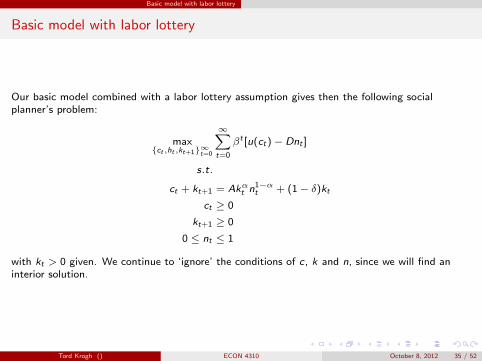
Our basic model combined with a labor lottery assumption gives then the following socialplanner’s problem:

max{ct ,ht ,kt+1}∞t=0

∞∑t=0

βt [u(ct )− Dnt ]

s.t.

ct + kt+1 = Akαt n1−αt + (1− δ)kt

ct ≥ 0

kt+1 ≥ 0

0 ≤ nt ≤ 1

with kt > 0 given. We continue to ‘ignore’ the conditions of c, k and n, since we will find aninterior solution.



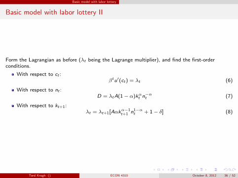
Basic model with labor lottery II

Form the Lagrangian as before (λt being the Lagrange multiplier), and find the first-orderconditions.

With respect to ct :βt u′(ct ) = λt (6)

With respect to nt :D = λt A(1− α)kαt n−αt (7)

With respect to kt+1:λt = λt+1[Aαkα−1

t+1 n1−αt + 1− δ] (8)



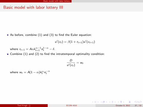
Basic model with labor lottery III

As before, combine (1) and (3) to find the Euler equation:

u′(ct ) = β(1 + rt+1)u′(ct+1)

where rt+1 = Aαkα−1t+1 n1−α

t − δ.

Combine (1) and (2) to find the intratemporal optimality condition:

D

u′(ct )= wt

where wt = A(1− α)kαt n−αt



Basic model with labor lottery IV

With n fixed (before today), optimum required the following conditions to be satisfied:

The Euler equation

The resource constraint

Introducing labor supply and making n be set optimally adds one extra restriction:

The intratemporal optimality condition



Basic model with labor lottery V

Next steps? Like in Lecture 11:

Characterize steady state

Linearize conditions around steady state

Solve the set of linearized equations

Plot impulse-response functions, simulate, calculate moments etc.

We can save this to next lecture.


Calibration

Calibration

One thing we will not save to next lecture is: How should we choose values for the structuralparameters in an RBC model? What is most frequently applied is called calibration.


Calibration

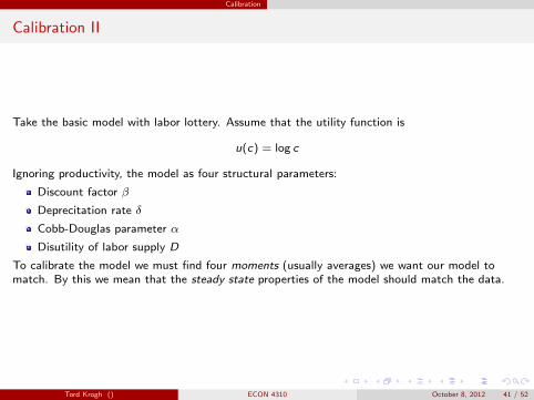
Calibration II

Take the basic model with labor lottery. Assume that the utility function is

u(c) = log c

Ignoring productivity, the model as four structural parameters:

Discount factor β

Deprecitation rate δ

Cobb-Douglas parameter α

Disutility of labor supply D

To calibrate the model we must find four moments (usually averages) we want our model tomatch. By this we mean that the steady state properties of the model should match the data.


Calibration

Calibration III

A standard set of moments to match are:

Average capital share of income

Average investment to capital ratio

Average long-term real interest rate

Average share of available hours spent on work

Let us see how we can use each of these moments to calibrate our model.


Calibration

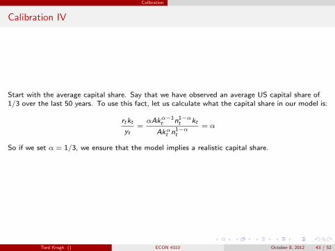
Calibration IV

Start with the average capital share. Say that we have observed an average US capital share of1/3 over the last 50 years. To use this fact, let us calculate what the capital share in our model is:

rt kt

yt=αAkα−1

t n1−αt kt

Akαt n1−αt

= α

So if we set α = 1/3, we ensure that the model implies a realistic capital share.


Calibration

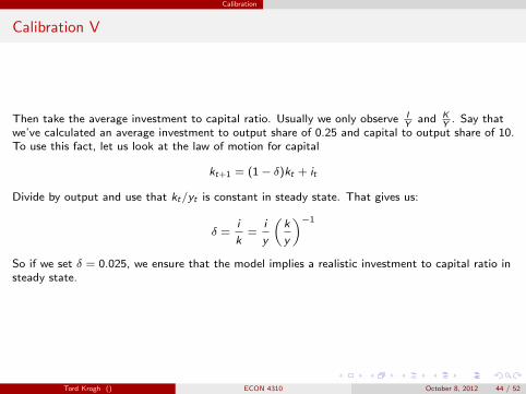
Calibration V

Then take the average investment to capital ratio. Usually we only observe IY

and KY

. Say thatwe’ve calculated an average investment to output share of 0.25 and capital to output share of 10.To use this fact, let us look at the law of motion for capital

kt+1 = (1− δ)kt + it

Divide by output and use that kt/yt is constant in steady state. That gives us:

δ =i

k=

i

y

(k

y

)−1

So if we set δ = 0.025, we ensure that the model implies a realistic investment to capital ratio insteady state.


Calibration

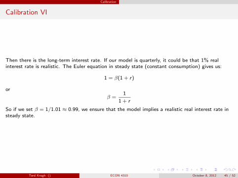
Calibration VI

Then there is the long-term interest rate. If our model is quarterly, it could be that 1% realinterest rate is realistic. The Euler equation in steady state (constant consumption) gives us:

1 = β(1 + r)

or

β =1

1 + r

So if we set β = 1/1.01 ≈ 0.99, we ensure that the model implies a realistic real interest rate insteady state.


Calibration

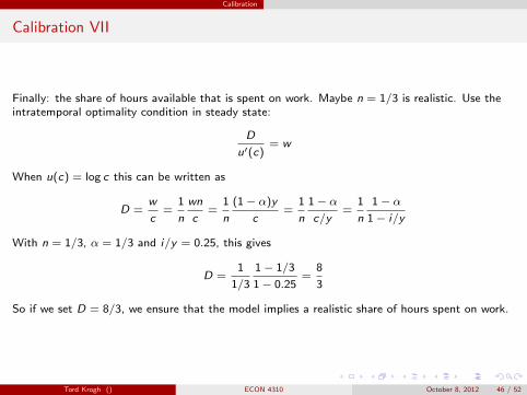
Calibration VII

Finally: the share of hours available that is spent on work. Maybe n = 1/3 is realistic. Use theintratemporal optimality condition in steady state:

D

u′(c)= w

When u(c) = log c this can be written as

D =w

c=

1

n

wn

c=

1

n

(1− α)y

c=

1

n

1− αc/y

=1

n

1− α1− i/y

With n = 1/3, α = 1/3 and i/y = 0.25, this gives

D =1

1/3

1− 1/3

1− 0.25=

8

3

So if we set D = 8/3, we ensure that the model implies a realistic share of hours spent on work.


Calibration

Calibration VIII

Summary? If we want to ensure a capital share equal to 1/3, an investment to capital ratio of2.5%, a real interest rate of 1% and n = 1/3 in our model we just choose:

α = 1/3

δ = 0.025

β = 1/1.01

D = 8/3


Calibration

Calibration IX

Calibrating the model in this way ensures that the model has reasonable long-run properties.

So it is not impressing that our RBC model manages to replicate these facts

The interesting question is: How well will a simple model calibrated to match long-run factsdo when it comes to explain business cycles?


Calibration

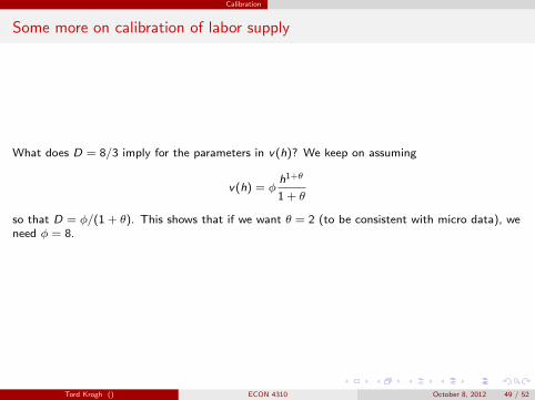
Some more on calibration of labor supply

What does D = 8/3 imply for the parameters in v(h)? We keep on assuming

v(h) = φh1+θ

1 + θ

so that D = φ/(1 + θ). This shows that if we want θ = 2 (to be consistent with micro data), weneed φ = 8.


Calibration

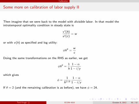
Some more on calibration of labor supply II

Then imagine that we were back to the model with divisible labor. In that model theintratemporal optimality condition in steady state is

v ′(h)

u′(c)= w

or with v(h) as specified and log utility:

φhθ =w

c

Doing the same transformations on the RHS as earlier, we get

φhθ =1

h

1− α1− i/y

which gives

φ =1

h1+θ

1− α1− i/y

If θ = 2 (and the remaining calibration is as before), we have φ = 24.


Calibration

Some more on calibration of labor supply III

So we could of course also calibrate a model with divisible labor to obtain h = 1/3 in steadystate. The effect is an implicit selection of a much larger value of φ.

But that does not change the main difference between the labor lottery and divisible labormodels: The difference in substitution effects!


Calibration

Three things you MUST remember from today

1 What is the Frisch elasticity?

2 Why do we use the labor lotteries model?

3 How do we choose values for the structural parameters in an RBC model?


labor supply in rbc models + calibration - forsiden ... supply in rbc models + calibration lecture...

Documents