labor contract law - arxiv.org · labor contract law—an economic view 3 / 24 introduction:...

1 / 24

Labor Contract Law

-An Economic View

Yaofeng FU*, Ruokun HUANG** and Yiran SHENG***

Department of Finance, School of Economics and Management,

Tsinghua University, Beijing, P. R. China

Abstract: China’s new labor law – Labor Contract Law has been put into practice for over one year.

Since its inception, debates have been whirling around the nation, if not the world. In this article,

we take an economic perspective to analyze the possible impact of the core item–open-ended

employment contract, and we find that it deals poorly with adverse selection, with moral hazard

problems arise, which fails to meet the expectations of law-makers and other parties.

Keyword: Open-ended contract, adverse selection, moral hazards, information asymmetry

Version: Apr 2009

* Yaofeng FU, [email protected], student ID 2006012405. ** Ruokun HUANG, [email protected], [email protected], student ID 2006012402. *** Yiran SHENG, [email protected], student ID 2006012400.

mailto:[email protected]




Labor Contract Law—An Economic View

2 / 24

Contents

Introduction: Overall Debates ........................................................................................................... 3

Economic Evaluation in Organizational Theory Approach ................................................................ 6

Section I A simple model: The methodology of firing employees ............................................ 7

Section II adverse selection ..................................................................................................... 10

One period model ........................................................................................................... 11

Two-period model ........................................................................................................... 11

Three-period model ........................................................................................................ 16

Challenges and further works to be done ....................................................................... 21

Section III Moral Hazard Problem ........................................................................................... 22

Policy Implications and International Experience ................................................................... 23

References ....................................................................................................................................... 24


3 / 24

Introduction: Overall Debates

The Labor Contract Law (hereafter referred as the Law) in China is enacted in

2007 and became effective on the first day of 2008. And the idea of this new

law was proposed in the year 2005. This new law enjoyed huge focus and

popularity nationwide with media coverage for every single article within it. It

was once reported that during the 28th Session of the Standing Committee of

the 10th National People's Congress, which took place on the day of 30th June

2007, the Law was passed with 145 pro-votes and 0 against-vote,

demonstrating a sharp contrast with laws and regulations passed before.

Another example of its popularity is the fact that around 200,000 of pieces of

suggestion were handed in within one month of open consulting from the public.

However, the popularity and majority concern cannot guarantee a perfect law.

In fact, the Law has long been a subject of debate over the years passed since

its inception.

The preliminary debate of this law comes from the fundamental concept within

the law. The basic idea is to protect the “disadvantaged labor” against the

“over-dominant” capital, which have made an indispensable contribution to

China’s economy since its open-up policy in 1979. On one hand, law makers

argue that migrant workers in China have never got the chance to protect their

own rights since the open-up, i.e. they got little symbolic “compensation” for

from the employers if they were hurt or even disabled during their work, and

even got nothing back at all, which is often the case, because they are not

officially hired by their employers – no contracts, no wage guarantee, not to

mention the insurance. On the other hand, economists argue that the law leans

towards the employees, which will results in the consequence of increasing the

labor costs of companies, thus making China losing the low-labor-cost

advantages, which has attracted tremendous amounts of investment from

abroad. As for economists, they believe that a better social welfare system is a

more practical way to tackle with the problems facing migrant workers, rather

than a change of law. And if necessary, the change of law should not deviate

from the stand of protecting both sides simultaneously.

The authors of this article agree with the latter point of view, not simply

because we are the potential economists in the future, but further, evidence

shows that the leaning-towards workers policy is not favorable to all the

workers as a whole, but only a small proportion of employees, who have already

been quite well-off because of their already highly accumulated human capital.

For those in lack of human capital or poor in skills, as in the case of most

migrant workers in China, this policy can create unexpected consequences for

those workers as law-makers cannot anticipate. The underlying mechanism lies


4 / 24

in the fact that the over-protective items in the Law make the employers more

cautious and hesitant when deciding on whether or not to hire a person,

especially in the cases where the job candidates are at the margin of being

accepted due to their not-that-high skills and experiences, making those, for

example, migrant workers lose the potential opportunities of employment

otherwise they would not lose. To summarize, the ideal of those law-makers

may appear noble, i.e. to protect “disadvantaged labor”, however, the impact

may well be the opposite to their intention due to their lack of knowledge of

economics of organizations.

Nowadays, the debate concentrates largely on two other issues instead: should

the law in China coerce employers to sign an open-ended employment contract

with their employees or not, and additionally, should those employers pay a

minimum wage for the workers. The specific items in the law are displayed as

follows:

Article 14 (open-ended contract): “If an Employee proposes or agrees to renew

his employment contract or to conclude an employment contract in any of the

following circumstances, an open-ended employment contract shall be

concluded, unless the Employee requests the conclusion of a fixed-term

employment contract.”

Article 20 (minimum wage rate): “The wages of an Employee on probation may

not be less than the lowest wage level for the same job with the Employer or

less than 80 percent of the wage agreed upon in the employment contract, and

may not be less than the minimum wage rate in the place where the Employer

is located.”

The debate between law-makers and economists centered much on the open-

ended employment contract, which is the core of the new Labor Contract Law

in China, and also the main achievement that law-makers are proud of. Both

sides are using seemingly well-grounded arguments to support their points.

The law-makers argue that the status quo of the labor-capital relation should

be re-established because the workers in China share a “natural” disadvantage

over their employers because of two reasons, one is the lack of effective labor

union (in fact, the union in China mainly concentrates on the internal affairs in

the organizations, rather than protecting the legal rights of the workers); the

other reason lies in the poor welfare system in China, leading to the lack of

proper compensation and protection against possible lay-off. The open-ended

employment contract, they argue, can solve these problems by offering better

protection to workers against this situation, and they often quote the increase

of the contract-signing percentage from less than 30% to 93% in the last year

as an evidence of benefits from the open-ended contracts. On the other side,

the economists, however, believe that this design of law twisted the incentive

of employers and employees as well, making the former less willing to hire and


5 / 24

the latter more “eager” to protect their legal rights, resulting in the

consequence of increasing unemployment. This argument cannot be verified

yet because the current financial crisis can contribute a lot towards the rise in

unemployment rate.

The debate of minimum wage rate among the two parties shows the similar

logic of reasoning, which involves the law-makers intended to protect the

workers, in probation or after being fired, while the economists criticized it

because of the twisted incentive problem.

In conclusion, authors of this article believe that the Labor Contract Law,

especially the articles in which open-ended employment contracts and

minimum wage rate, has brought more harm than benefits to the workers

involved, and the reasons for the argument are as follows: the costs of

employment for companies increase, making them unwilling to hire; on the

other side, the workers have no high incentive to accumulate their human

capital, rather, they will focus on taking legal actions against employers. Both

of these will result in the inflexibility of employment and unemployment,

especially for the “disadvantaged” groups, such as migrant workers, women,

new graduates from college etc., who are supposed to be protected, rather than

harmed.


6 / 24

Economic Evaluation in Organizational

Theory Approach

One of the elementary goals of the new labor contract aims at is making

businesses responsible for fairness and equality in the economy. This is

questioned, if not totally rejected, by modern economic theories. Businesses’

key issue is productivity, inefficient businesses will reduce benefits or close

their doors entirely, an outcome undesirable to the whole society as it leads to

higher unemployment and very likely, greater unfairness.

Various theoretical approaches can be taken to address such issues in detail,

this article focuses on those based on the organizational theories we have

studied in this course. In specific, we address the informational problems arise

from the new restrictions regarding the labor contract terms the LAW imposed

on businesses. Adverse selection and moral hazard issues are analyzed in the

following paragraphs.

Our topic derives from Chapter 3, Article 14, in the LAW, which is stated as

follows:

An Employer and an Employee may conclude an open-ended employment contract upon

reaching a negotiated consensus. If an Employee proposes or agrees to renew his employment

contract or to conclude an employment contract in any of the following circumstances, an

open-ended employment contract shall be concluded, unless the Employee requests the

conclusion of a fixed-term employment contract:

(3)Prior to the renewal, a fixed-term employment contract was concluded on two consecutive

occasions and the Employee is not characterized by any of the circumstances set forth in

Article 39 and items (1) and (2) of Article 40 hereof.

Productivity is the critical concept to understand businesses’ behavior, thus

making information structure of workers’ productivity very essential while

discussing the effectiveness of this item in the LAW. In the following analysis,

we use traditional informational economics concepts, i.e. adverse selection and

moral hazard to emphasize possible market distortions the LAW would

potentially bring. Then, we will discuss a few additional topics regarding

macroeconomic conditions and international experiences, which are quite

important in evaluating the LAW, yet have relative little relevance to our course.


7 / 24

Section I A simple model: The methodology of firing

employees

We are going to give an explanation of how firms fire workers. We claim that

firm cannot observe the true productivity of workers in single period, as what

was assumed in the model in class. We assume that the observation process

need more than one period, by the following model:

Assumption 1

Firm cannot tell the exact productivity of a worker, but can confirm that

(100% confidence level) the productivity are in a particular interval, or

, 1iP a b

Assumption 2

The firm at each period can only discover the relatively some worst workers

(in some interval), or

We can surely distinguish from

,

,

i

i

a c

c b

.

Assumption 3

The firm fire workers, or the workers quit, when the firm discover the worker

,i a c and that c .

Assumption 4

The workers are uniformly distributed from ,l h . The firm at period t can

only observe surely 1

,i l h l l h l

t t

n n

or surely

1

,i l h l h

t

n

. Thus it needs n periods to entirely discover the

workers’ productivity.

Object: Firm wants to hire workers with high productivity.


8 / 24

Model:

When there are n periods, there is one worker work for the firm. If the firm

discovers the employee’s productivity falls in the dark area, he would be fired,

in corresponding period.

The firm fire unqualified workers, whose productivity is less then market

average, step by step from 1st period to jth period, where the remaining workers’

productivity are all above market average.

When there are less than n periods available, say m periods, for a firm to justify

and fire workers,

1st-prd

2nd-prd

3rd-prd

jth-prd


9 / 24

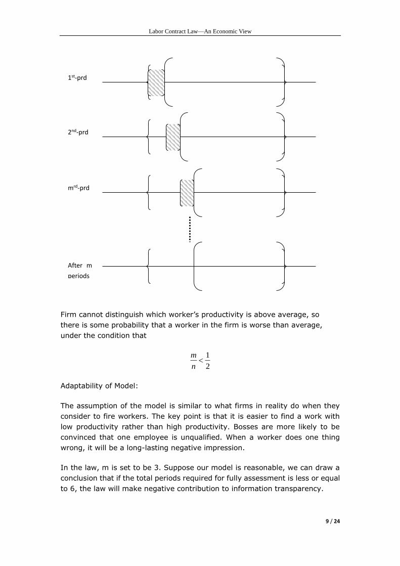
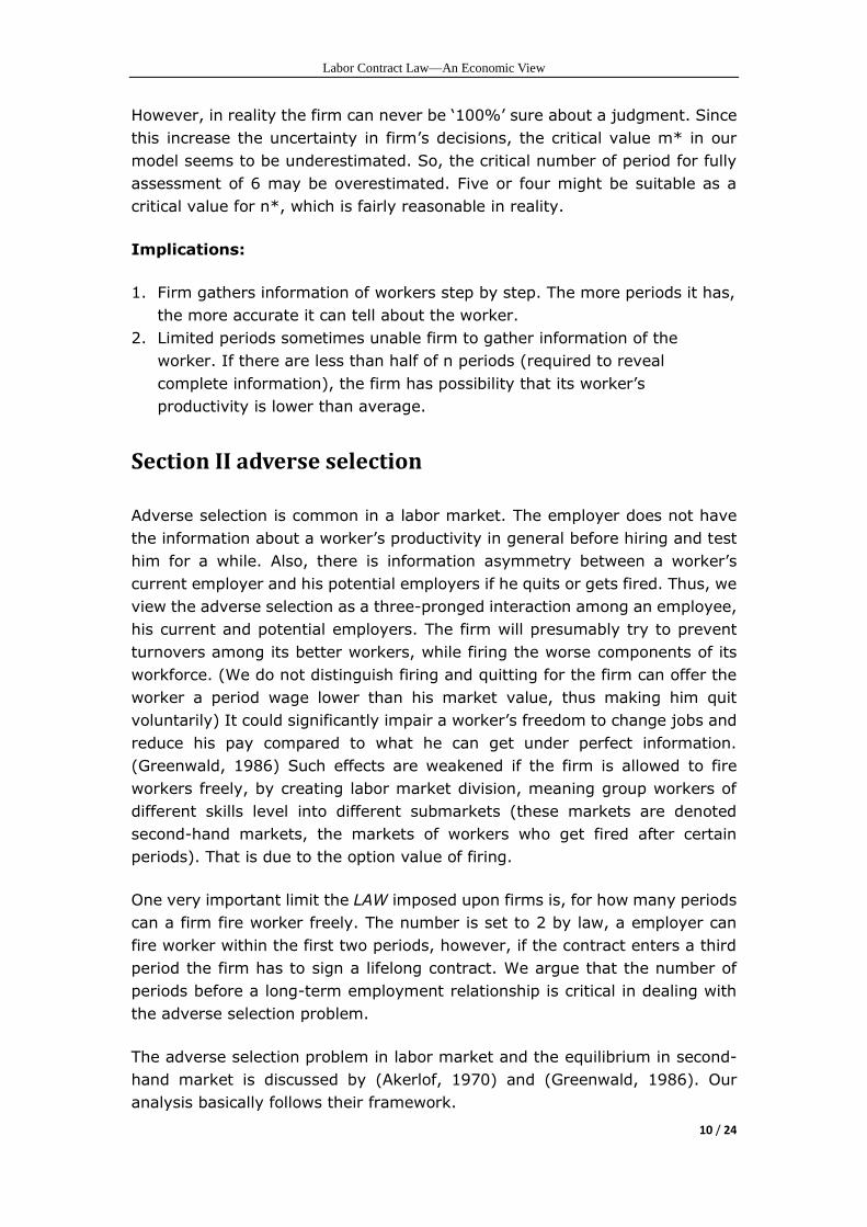
Firm cannot distinguish which worker’s productivity is above average, so

there is some probability that a worker in the firm is worse than average,

under the condition that

1

2

m

n

Adaptability of Model:

The assumption of the model is similar to what firms in reality do when they

consider to fire workers. The key point is that it is easier to find a work with

low productivity rather than high productivity. Bosses are more likely to be

convinced that one employee is unqualified. When a worker does one thing

wrong, it will be a long-lasting negative impression.

In the law, m is set to be 3. Suppose our model is reasonable, we can draw a

conclusion that if the total periods required for fully assessment is less or equal

to 6, the law will make negative contribution to information transparency.

1st-prd

2nd-prd

mrd-prd

After m

periods


10 / 24

However, in reality the firm can never be ‘100%’ sure about a judgment. Since

this increase the uncertainty in firm’s decisions, the critical value m* in our

model seems to be underestimated. So, the critical number of period for fully

assessment of 6 may be overestimated. Five or four might be suitable as a

critical value for n*, which is fairly reasonable in reality.

Implications:

1. Firm gathers information of workers step by step. The more periods it has,

the more accurate it can tell about the worker.

2. Limited periods sometimes unable firm to gather information of the

worker. If there are less than half of n periods (required to reveal

complete information), the firm has possibility that its worker’s

productivity is lower than average.

Section II adverse selection

Adverse selection is common in a labor market. The employer does not have

the information about a worker’s productivity in general before hiring and test

him for a while. Also, there is information asymmetry between a worker’s

current employer and his potential employers if he quits or gets fired. Thus, we

view the adverse selection as a three-pronged interaction among an employee,

his current and potential employers. The firm will presumably try to prevent

turnovers among its better workers, while firing the worse components of its

workforce. (We do not distinguish firing and quitting for the firm can offer the

worker a period wage lower than his market value, thus making him quit

voluntarily) It could significantly impair a worker’s freedom to change jobs and

reduce his pay compared to what he can get under perfect information.

(Greenwald, 1986) Such effects are weakened if the firm is allowed to fire

workers freely, by creating labor market division, meaning group workers of

different skills level into different submarkets (these markets are denoted

second-hand markets, the markets of workers who get fired after certain

periods). That is due to the option value of firing.

One very important limit the LAW imposed upon firms is, for how many periods

can a firm fire worker freely. The number is set to 2 by law, a employer can

fire worker within the first two periods, however, if the contract enters a third

period the firm has to sign a lifelong contract. We argue that the number of

periods before a long-term employment relationship is critical in dealing with

the adverse selection problem.

The adverse selection problem in labor market and the equilibrium in second-

hand market is discussed by (Akerlof, 1970) and (Greenwald, 1986). Our

analysis basically follows their framework.


11 / 24

The model

Under symmetry information, each worker is hired and paid according to his

real productivity, that is wi = θi, the former term denotes his wage, and the

latter term his productivity.

Under asymmetry information, we build up three models with the different

periods within which firms could fire workers freely.

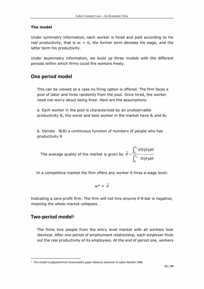
One period model

This can be viewed as a case no firing option is offered. The firm faces a

pool of labor and hires randomly from the pool. Once hired, the worker

need not worry about being fired. Here are the assumptions.

a. Each worker in the pool is characterized by an unobservable

productivity θi, the worst and best worker in the market have θL and θH

b. Denote N(θ) a continuous function of numbers of people who has

productivity θ

The average quality of the market is given by

( )

( )

H

L

H

L

N d

N d

In a competitive market the firm offers any worker it hires a wage level:

w* =

Indicating a zero-profit firm. The firm will not hire anyone if θ-bar is negative,

meaning the whole market collapses.

Two-period model1

The firms hire people from the entry level market with all workers look

identical. After one period of employment relationship, each employer finds

out the real productivity of its employees. At the end of period one, workers

1 This model is adjusted from Greenwald’s paper Adverse Selection in Labor Market 1986.


12 / 24

are offered 2 options. They can either stay with their current employers or

change jobs. In the latter event, they enter a second hand market.

We carry out the same assumptions from 1-period model, to describe the

basic structure of entry level market. Addition assumptions regarding the

second-hand market are as follows:

Assumption c: Employers in the second-hand market have no more

information other than the workers’ employment history to infer the

productivity of its potential workers.

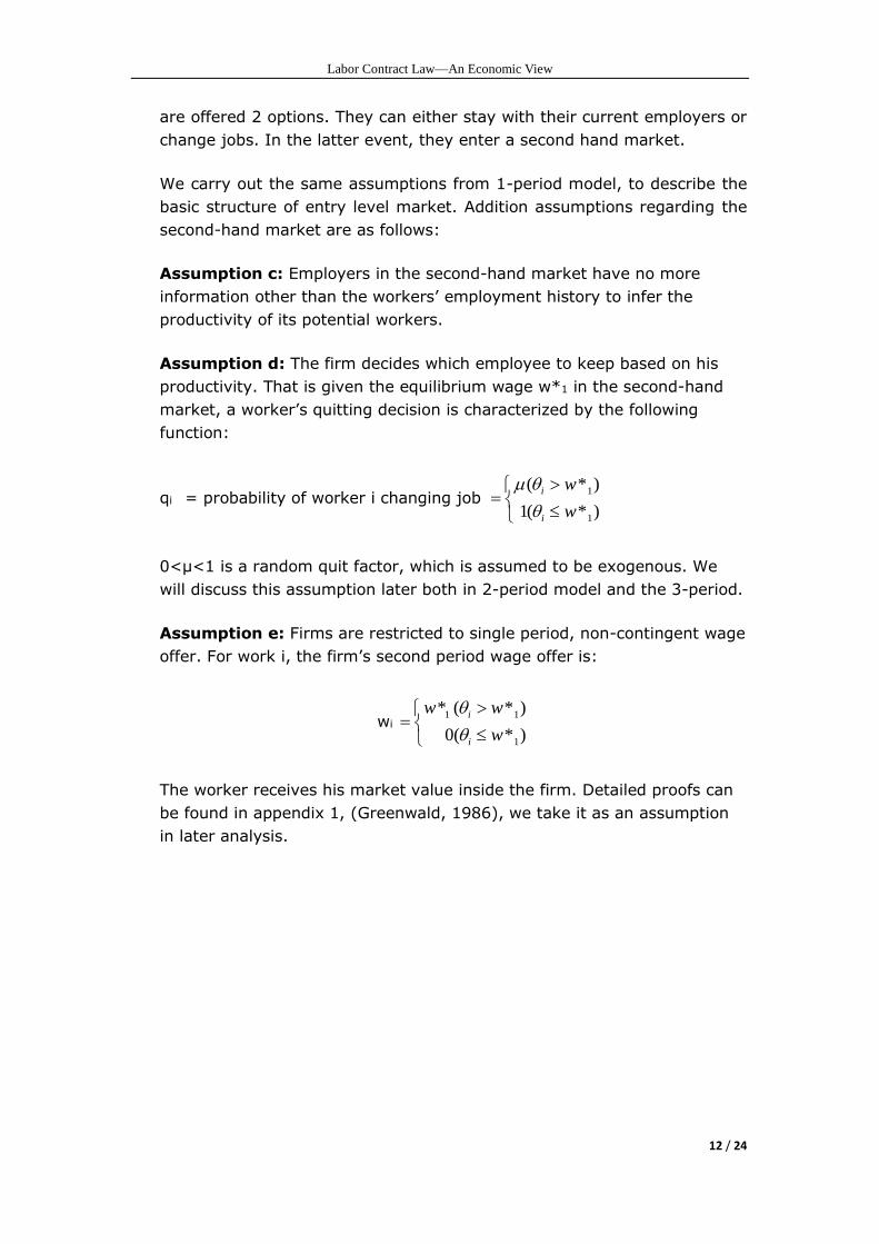
Assumption d: The firm decides which employee to keep based on his

productivity. That is given the equilibrium wage w*1 in the second-hand

market, a worker’s quitting decision is characterized by the following

function:

qi = probability of worker i changing job 1

1

( * )

1( * )

i

i

w

w

0<μ<1 is a random quit factor, which is assumed to be exogenous. We

will discuss this assumption later both in 2-period model and the 3-period.

Assumption e: Firms are restricted to single period, non-contingent wage

offer. For work i, the firm’s second period wage offer is:

wi 1 1

1

* ( * )

0( * )

i

i

w w

w

The worker receives his market value inside the firm. Detailed proofs can

be found in appendix 1, (Greenwald, 1986), we take it as an assumption

in later analysis.


13 / 24

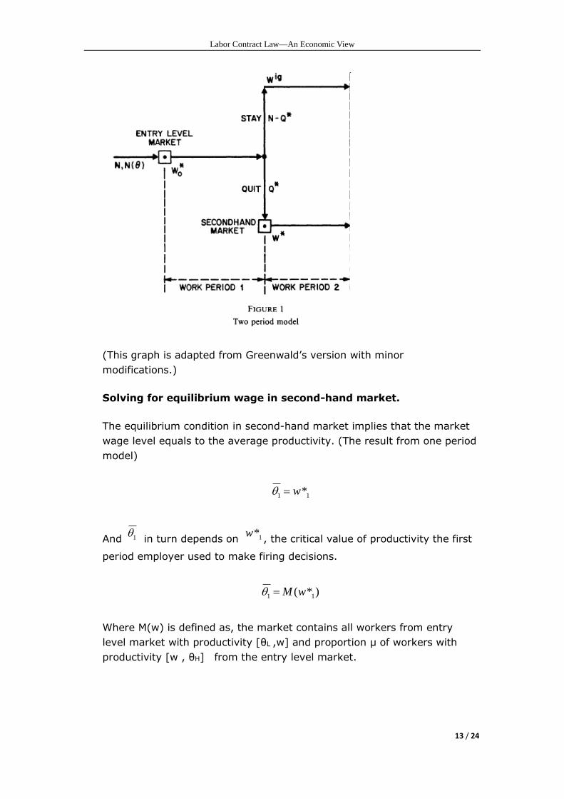
(This graph is adapted from Greenwald’s version with minor

modifications.)

Solving for equilibrium wage in second-hand market.

The equilibrium condition in second-hand market implies that the market

wage level equals to the average productivity. (The result from one period

model)

1 1*w

And 1 in turn depends on 1*w, the critical value of productivity the first

period employer used to make firing decisions.

1 1( * )M w

Where M(w) is defined as, the market contains all workers from entry

level market with productivity [θL ,w] and proportion μ of workers with

productivity [w , θH] from the entry level market.


14 / 24

( ) ( )( )

( ) ( )

H

L

H

L

w

w

w

w

N d N dM w

N d N d

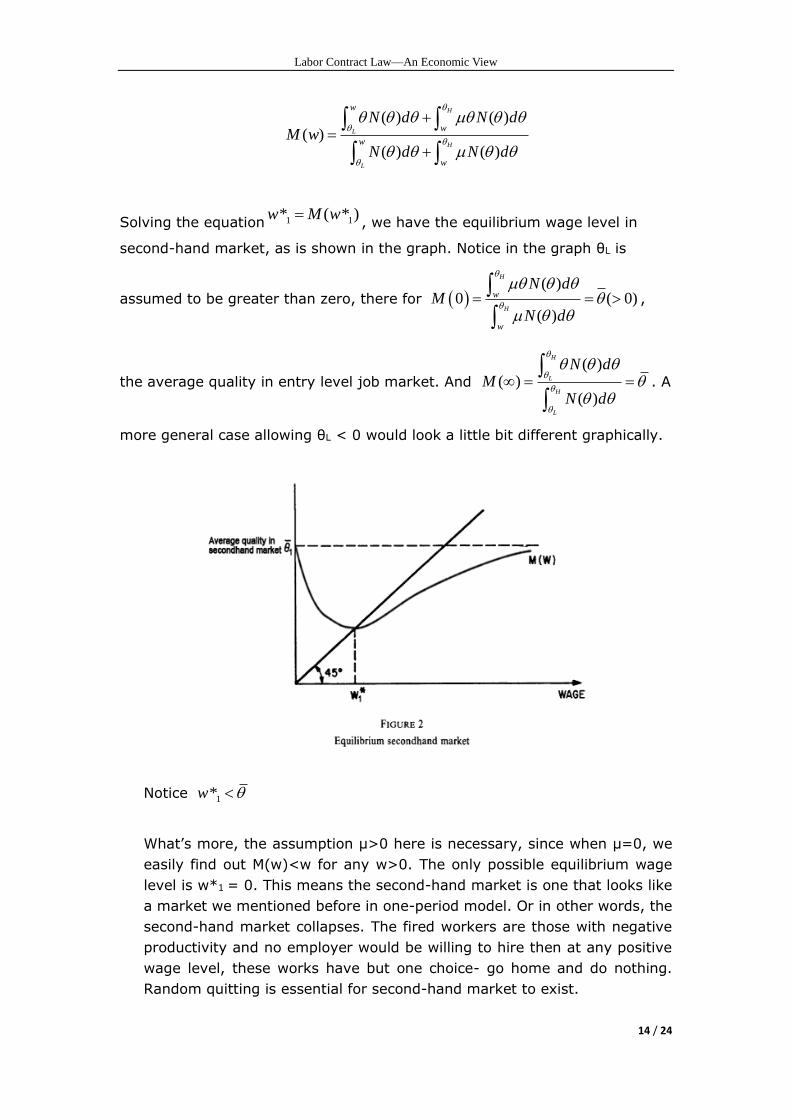
Solving the equation 1 1* ( * )w M w, we have the equilibrium wage level in

second-hand market, as is shown in the graph. Notice in the graph θL is

assumed to be greater than zero, there for ( )

0 ( 0)( )

H

H

w

w

N dM

N d

,

the average quality in entry level job market. And ( )

( )( )

H

L

H

L

N dM

N d

. A

more general case allowing θL < 0 would look a little bit different graphically.

Notice 1*w

What’s more, the assumption μ>0 here is necessary, since when μ=0, we

easily find out M(w)<w for any w>0. The only possible equilibrium wage

level is w*1 = 0. This means the second-hand market is one that looks like

a market we mentioned before in one-period model. Or in other words, the

second-hand market collapses. The fired workers are those with negative

productivity and no employer would be willing to hire then at any positive

wage level, these works have but one choice- go home and do nothing.

Random quitting is essential for second-hand market to exist.


15 / 24

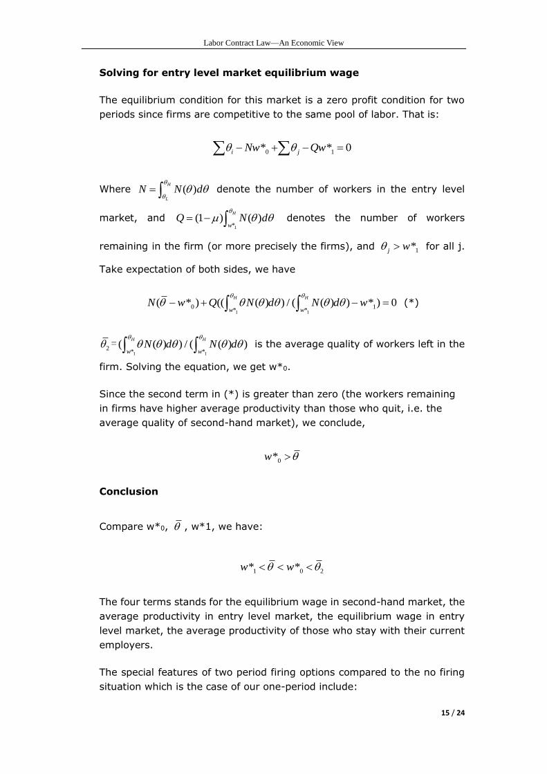
Solving for entry level market equilibrium wage

The equilibrium condition for this market is a zero profit condition for two

periods since firms are competitive to the same pool of labor. That is:

0 1* * 0i jNw Qw

Where ( )H

L

N N d

denote the number of workers in the entry level

market, and 1*

(1 ) ( )H

wQ N d

denotes the number of workers

remaining in the firm (or more precisely the firms), and 1*j w for all j.

Take expectation of both sides, we have

1 10 1

* *( * ) (( ( ) ) / ( ( ) ) * ) 0

H H

w wN w Q N d N d w

(*)

2 =1 1* *

( ( ) ) / ( ( ) )H H

w wN d N d

is the average quality of workers left in the

firm. Solving the equation, we get w*0.

Since the second term in (*) is greater than zero (the workers remaining

in firms have higher average productivity than those who quit, i.e. the

average quality of second-hand market), we conclude,

0*w

Conclusion

Compare w*0, , w*1, we have:

1 0 2* *w w

The four terms stands for the equilibrium wage in second-hand market, the

average productivity in entry level market, the equilibrium wage in entry

level market, the average productivity of those who stay with their current

employers.

The special features of two period firing options compared to the no firing

situation which is the case of our one-period include:


16 / 24

1. For an entry level market with <0, the one period model suggests

there will be no market at all, the workers with positive productivity as

well as the firms will suffer. Within the framework of 2-period model, on

the other hand, the firm will hire from such an negative expected

productivity market as long as the firm can fire those bad workers at the

end of period 1 and keep the good workers and pay them the same as

(perhaps a little bit more) the bad workers’ wage in the second-hand

market, in this case it is 0 (w*1< <0). There will exist a positive

equilibrium wage w*0 in the entry level market, sufficiently large over

. A simplified version of this model is provided in Chapter 3 of our

textbook of this course.

2. Since w*0 is driven up by market competition, there will be free riders in

the entry level market. The bad workers enjoy a high 1st period wage at

the expanse of shrank pay of the good workers. The good workers are

compensated in period 1, but their pay is significantly undermined in the

2nd period, for they are not able to prove their true productivity in the

second-hand market, thus trapped with their current employer and

receive a low pay (w*1) compared to their high productivity( 2 ).

The two-period and 1st period end option of firing manage to solve some

problems but still, the fundamental issues of adverse selection remain

unresolved. What would be a better solution? A 3-period needs to be forged

to answer this question. Now we know the 2-period case provide the first-

degree division of labor markets by creating a second-hand market, and

distinguish the bad workers from the entire work force. If employer is

allowed to fire workers at the end of period 2 before entering into a period

3 (a long-term contract), the labor market will be divided further into 3

second-hand markets, and information regarding workers’ real productivity

is better revealed and classified. This regime is what the LAW offers to the

economy while the old system is even more flexible with infinite periods and

free firing option at the end of each period.

Three-period model

The model follows the same set of assumptions in the previous discussion.

In addition, one more assumption is required here:


17 / 24

Assumption f: Firms have perfect information of a worker’s employment

history. 2

Mathematical notations are carried out as follows.

the average productivity in entry level market

N(θ) the number of workers with productivity θ in entry level market

N The number of workers in the entry level market

N1,Q1 The number of workers in the second market, and the number of

workers who remain with their current employers the end of the

1st period

N2,Q2 The number of workers in the third market, and the number of

workers who stay with their current employers the end of the 2nd

period

N2’,Q2’ The number of workers in the double second market, and the

number of workers who stay with their current employers the end

of the 2nd period

w*0 The equilibrium wage level in the entry level market

w*1 The equilibrium wage level in the second market

w*+ The wage the workers receive who choose to stay with their

current employer after period 1, notice w*+ and w*1 don’t have to

be equal

w*2 The equilibrium wage level in the third market

w*2’ The equilibrium wage level in the double second market

Note the second market means the labor market for laid-off workers at the

end of the first period, and the third market is the market for laid-off

workers at the end of the second period. And the double second market is

the market of twice fired workers at the end of the second period.

2 Here is our major distinction compared to Greenald’s work (1986), which assumes all laid-off workers just enters into a same second-hand market. However, assumption f in our model implies different workers with different employment history are automatically grouped into four sub-markets based on the whether and when they change their job. The four markets and its definition can be found on the next page.


18 / 24

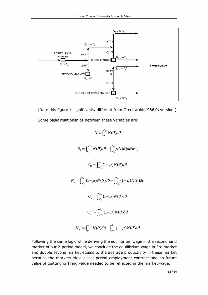
(Note this figure is significantly different from Greenwald(1986)’s version.)

Some basic relationships between these variables are:

( )H

L

N N d

1

*

1*

( ) ( ) *H

L

w

wN N d N d w

1*

(1 ) ( )H

wQ N d

22

* * '(1 ) ( ) (1 ) ( )

H H

w wN N d N d

22

*(1 ) ( )

H

wQ N d

22

* '' (1 ) ( )

H

wQ N d

2

*

2* '

' ( ) (1 ) ( )H

L

w

wN N d N d

Following the same logic while deriving the equilibrium wage in the secondhand

market of our 2-period model, we conclude the equilibrium wage in 3rd market

and double second market equals to the average productivity in these market

because the markets yield a last period employment contract and no future

value of quitting or firing value needed to be reflected in the market wage.


19 / 24

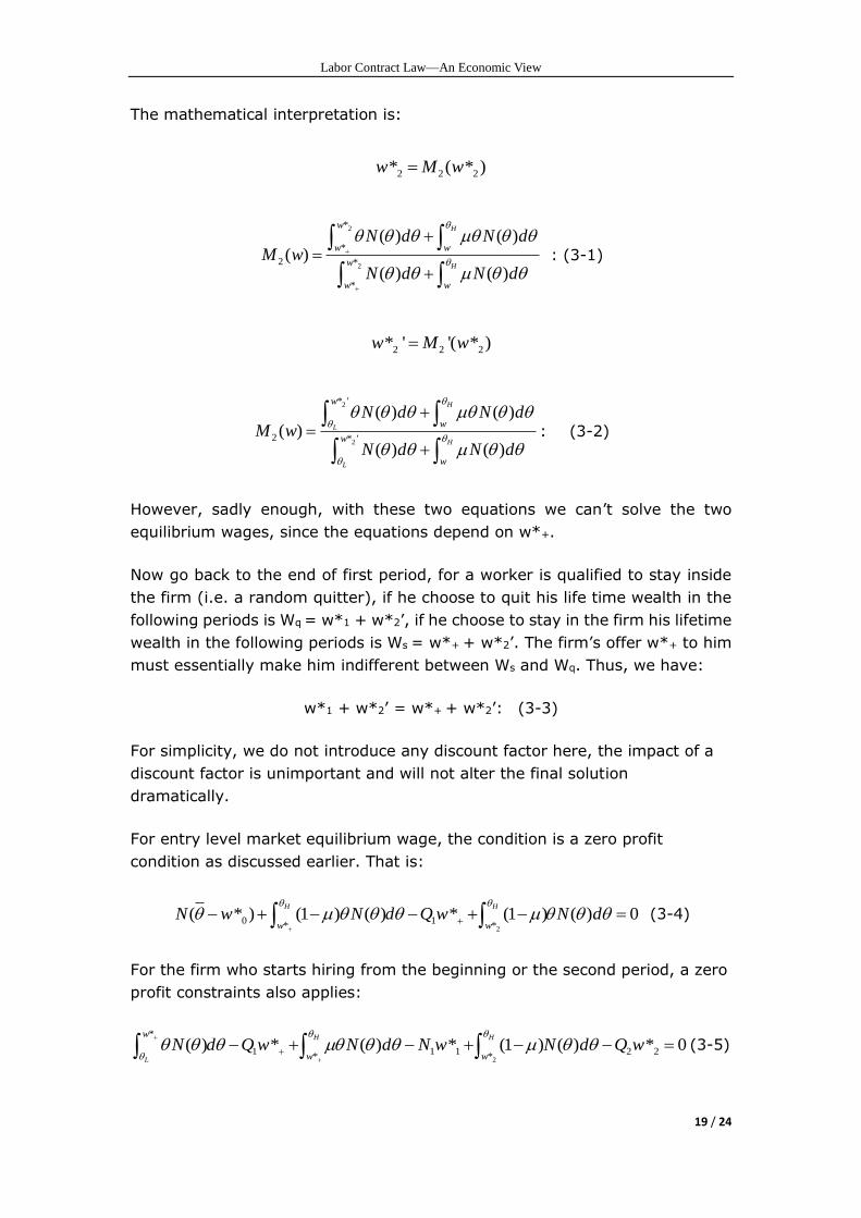
The mathematical interpretation is:

2 2 2* ( * )w M w

2

2

*

*

2 *

*

( ) ( )( )

( ) ( )

H

H

w

w w

w

w w

N d N dM w

N d N d

: (3-1)

2 2 2* ' '( * )w M w

2

2

* '

2 * '

( ) ( )( )

( ) ( )

H

L

H

L

w

w

w

w

N d N dM w

N d N d

: (3-2)

However, sadly enough, with these two equations we can’t solve the two

equilibrium wages, since the equations depend on w*+.

Now go back to the end of first period, for a worker is qualified to stay inside

the firm (i.e. a random quitter), if he choose to quit his life time wealth in the

following periods is Wq = w*1 + w*2’, if he choose to stay in the firm his lifetime

wealth in the following periods is Ws = w*+ + w*2’. The firm’s offer w*+ to him

must essentially make him indifferent between Ws and Wq. Thus, we have:

w*1 + w*2’ = w*+ + w*2’: (3-3)

For simplicity, we do not introduce any discount factor here, the impact of a

discount factor is unimportant and will not alter the final solution

dramatically.

For entry level market equilibrium wage, the condition is a zero profit

condition as discussed earlier. That is:

20 1

* *( * ) (1 ) ( ) * (1 ) ( ) 0

H H

w wN w N d Q w N d

(3-4)

For the firm who starts hiring from the beginning or the second period, a zero

profit constraints also applies:

2

*

1 1 1 2 2* *

( ) * ( ) * (1 ) ( ) * 0H H

L

w

w wN d Q w N d N w N d Q w

(3-5)


20 / 24

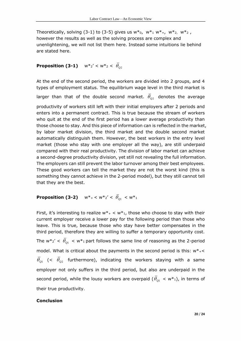
Theoretically, solving (3-1) to (3-5) gives us w*0, w*1 w*+, w*2, w*2 ,

however the results as well as the solving process are complex and

unenlightening, we will not list them here. Instead some intuitions lie behind

are stated here.

Proposition (3-1) w*2’ < w*2 < 2Q

At the end of the second period, the workers are divided into 2 groups, and 4

types of employment status. The equilibrium wage level in the third market is

larger than that of the double second market. 2Q denotes the average

productivity of workers still left with their initial employers after 2 periods and

enters into a permanent contract. This is true because the stream of workers

who quit at the end of the first period has a lower average productivity than

those choose to stay. And this piece of information can is reflected in the market,

by labor market division, the third market and the double second market

automatically distinguish them. However, the best workers in the entry level

market (those who stay with one employer all the way), are still underpaid

compared with their real productivity. The division of labor market can achieve

a second-degree productivity division, yet still not revealing the full information.

The employers can still prevent the labor turnover among their best employees.

These good workers can tell the market they are not the worst kind (this is

something they cannot achieve in the 2-period model), but they still cannot tell

that they are the best.

Proposition (3-2) w*+ < w*2’ < 1Q < w*1

First, it’s interesting to realize w*+ < w*1, those who choose to stay with their

current employer receive a lower pay for the following period than those who

leave. This is true, because those who stay have better compensates in the

third period, therefore they are willing to suffer a temporary opportunity cost.

The w*2’ < 1Q < w*1 part follows the same line of reasoning as the 2-period

model. What is critical about the payments in the second period is this: w*+<

1Q (< 2Q furthermore), indicating the workers staying with a same

employer not only suffers in the third period, but also are underpaid in the

second period, while the lousy workers are overpaid ( 1Q < w*1), in terms of

their true productivity.

Conclusion


21 / 24

To summarize, the internal mechanism of labor productivity division has lagged

effects upon wage payments. After distinguish good and bad workers, the

employer has no incentive to offer the good one better pay consistent with his

real productivity, since the worker cannot prove himself so good if he quit, and

thus receives a wage outside measures the average productivity of a pool of

workers worse than him. The worker has to wait one more period to enjoy a

wage rise (only if the addition period exists). The 2-period mechanism achieves

a 1st-degree productivity distinction and 0-degree wage distinction. The 3-

period mechanism achieves a 2nd-degree productivity distinction and a 1st-

degree wage distinction. If we were to build up a n-period model, the results

will be the same. The adverse selection problem is dealt better if more periods

are offered, but never perfectly. The good workers are better when period’s

numbers increase, but they are always underpaid, only the gap becomes

narrower. Information advantage a current employer possesses gives them the

ex. post power to undermine good employees’ wage, thus benefits in a sense

of lower production costs. This in not parato optimal, obviously. However, ex.

ante competition among employers tends to drive up the upper branch of labor

market equilibrium wage. The relative bad workers receive a better pay at the

cost of a steep under-payment of the good workers in terms of productivity.

The first best solution of perfect information case is never feasible, but can be

approached through the increasing of period’s numbers.

Challenges and further works to be done

1. The only dimension we used to compare 2 and 3-period mechanisms is the

degree of divisions of productivity and wage payments. We say any finite

periods mechanisms cannot achieve a first-best (Pareto optimal) solution,

with only limited improvements offered. However, the welfare

improvements is not provided in the above theory, i.e. compare w*0 + w*2

+ w*+ of the 3-period model with the w*0 + w*1 of the 2-period model. This

is not insignificant in any case, but due to our limited mathematical skills in

solving (3-1) to (3-5), such comparison is not provided. Further study on

this issue should be carried out.

2. The assumption of random quit is not valid as period’s number increases.

We treat the quit rate in different periods as fixed and exogenous, while in

reality the rates could differ significantly across periods. Also, the

exogenous assumption is in question; a better approach should treat μ as

an endogenous variable, a variable the work force as a whole could choose

to maximize their utility. The change could have significant impact upon the

size of different divisions of labor markets.

3. The concept of divisions of labor market itself is not fully consistent with

reality. By some easy calculation, we found the number of sub-markets is


22 / 24

12 1n for n-period model, increasing at a geometric rate. The transaction

costs associated with such an incredible rate is dramatic. Thus it is quite

reasonable to doubt the actual effects we expected to see of labor markets

division as a well the likelihood of such a delicate division happens.

Based on these challenges, it is almost certain that an infinite periods approach

will not bring about too much exciting solution; for one thing, it fails to achieve

a parato efficient outcome, for another, its theoretical effectiveness is quite

limited due to unrealistic assumptions.

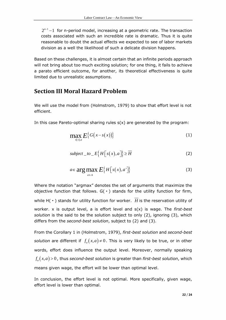
Section III Moral Hazard Problem

We will use the model from (Holmstrom, 1979) to show that effort level is not

efficient.

In this case Pareto-optimal sharing rules s(x) are generated by the program:

,

maxs x a

G x s xE (1)

_ _ ,subject to E H s x a H (2)

'

, 'argmaxa A

a H s x aE

(3)

Where the notation “argmax” denotes the set of arguments that maximize the

objective function that follows. G(·) stands for the utility function for firm,

while H(·) stands for utility function for worker. H is the reservation utility of

worker. x is output level, a is effort level and s(x) is wage. The first-best

solution is the said to be the solution subject to only (2), ignoring (3), which

differs from the second-best solution, subject to (2) and (3).

From the Corollary 1 in (Holmstrom, 1979), first-best solution and second-best

solution are different if , 0af x a . This is very likely to be true, or in other

words, effort does influence the output level. Moreover, normally speaking

, 0af x a , thus second-best solution is greater than first-best solution, which

means given wage, the effort will be lower than optimal level.

In conclusion, the effort level is not optimal. More specifically, given wage,

effort level is lower than optimal.


23 / 24

Policy Implications and International Experience

The open-ended employment contract introduced by the LAW, fixed the free

trial periods number to two, within which the employer can make hiring and

firing decisions independently. The key point here is to protect the workers’

rights while allowing the firms some degree of freedom to hire and select good

workers and fire those with relatively low productivity: a tradeoff between

efficiency and equality.

However, as we argued, with adverse selection problems in presence, the

number of periods the employers have allowing for free employment decisions

is critical in achieving the goal of efficiency, namely reducing adverse selection

to an acceptable level. The procedure introduced by the LAW is characterized

by our 3-period model in section II. And a 2-period free trial is definitely not

enough. Not only in a sense that adverse selection is merely roughly dealt (with

one 1st-degree of compensating identification accomplished), but also in a

manner equality is promoted poorly (significant underpay for the high-end

workers). In fact, as we argued, the inequality arises in labor contract is

preliminarily caused by the adverse selection, i.e. the employer is able to

undermine the compensation to its best workers, who cannot prove their real

productivity to the market due to information asymmetry. In this regard,

eliminating adverse selection and promoting equality become a same goal, yet

the solution offered by the LAW deals with both poorly.

Furthermore, we pointed out the old mechanism existing prior to the LAW,

offering infinite intervals of free trial, also has its limitations. First of all, it

cannot eliminate adverse selection and achieve the first-best solution in perfect

information case, however large the period’s number n is. Also, the

effectiveness of increasing period’s number declines dramatically due to factors

we mentioned at the end of section II. Therefore, returning to the old Labor

Contract Law is also not a good idea. If period’s number prior to open-ended

contract is the only policy tool available to us, the optimal number should be

worked out carefully rather than set to a roughly chosen one.

Also we took into consideration of potential moral hazard problems. The

workers’ incentive to diligent working is weakened, if not significantly distorted,

since the fear to lose jobs resolves once they enter into an open-ended contract

and the employer cannot fire them at will. Unlike adverse selection, which

generally exists before the introduction of the LAW, this problem is exactly

newly brought up the LAW. As there is no ideal theoretical mechanism we can

adapt to deal with moral hazard, we conclude this is one of the unnecessary

costs the LAW generated with no evident benefits created at the same time.


24 / 24

Therefore, we are confident to say the LAW failed to meet its initial expectation

and to satisfy its original goodwill.

In an international perspective, we found Germany and India once had laws

issued with similar content written inside, imposing constraints on firms’ hiring

and firing decisions. Countries with these kinds of laws—Germany, Italy, France,

India and some parts of Canada—bear higher unemployment rates, around nine

and ten percent. This does not include workers leaving these countries and

those not registered, so the true number may be twice the unemployment rate.

However, the countries without these kinds of laws have rates of four or five

percent.

Germany issued a law called co-determination which demanded the businesses’

decisions, arrangements and work conditions should be decided and agreed

both by the employees and the employers. Under this law, the businesses could

not fire any workers unless it was agreed to by the latter. Generally speaking,

the workers could not be fired after they were 40 years old. Eventually,

Germany’s labor market lacked of competitive strength, hurting the economy.

The Industrial Disputes Act (IDA) of India, passed in 1947, set the form of

mediation between employers and employees. The law also states that when a

business wants to fire more than 100 employees, it needs government approval.

Businesses in India found it difficult to fire workers after the law came into

effect.

To sum up, the study of employment contract is still in progress in the world,

and no strong results or explicit implications are made.

References

Akerlof, G. A. (1970, 8). The Market for 'Lemons': Quality Uncertainty and the Market Mechanism.

The Quarterly Journal of Economics , 3 (84), pp. 488-500.

Greenwald, B. C. (1986, 7). Adverse Selection in the Labour Market. The Review of Economic

Studies , pp. 325-347.

Holmstrom, B. (1979). Moral Hazard and Observability. The Bell Journal of Economics , 10 (1), pp.

74-91.

labor contract law - arxiv.org · labor contract law—an economic view 3 / 24 introduction:...

Documents