Koszul Algebras, Castelnuovo-Mumford Regularity, and Generic InitialIdeals

by

Giulio Caviglia

Submitted to the Department of Mathematics

and the Faculty of the Graduate School

of the University of Kansas

in partial fulfillment of the requirements

for the degree of Doctor of Philosophy

Thesis Committee:

Professor Craig Huneke, Chair

Professor Arvin Agah

Professor Rober Brown

Professor Daniel Katz

Professor Bangere Purnaprajna

c© Copyright 2004

by

Giulio Caviglia

All Rights Reserved

ii

Abstract

KOSZUL ALGEBRAS, CASTELNUOVO-MUMFORD REGULARITY, AND

GENERIC INITIAL IDEALS

Giulio Caviglia

The University of Kansas

Advisor: Craig Huneke

August, 2004

The central topics of this dissertation are: Koszul Algebras, bounds for the Castel-

nuovo Mumford regularity, and methods involving the use of generic changes

of coordinates and generic hyperplane restrictions. We give an introduction to

Koszul algebras and prove some criteria to show that an algebra is Koszul. We

use these methods to show that the Pinched Veronese, i.e. the toric ring defined as

K[X3,X2Y,XY 2,Y 3,X2Z,Y 2Z,XZ2,Y Z2,Z3], is Koszul.

The middle chapters are devoted to the Castelnuovo-Mumford regularity. We

give a collection of techniques and formulas to compute the regularity by using

hyperplane sections. For example we obtain some variations of a criterion due to

Bayer and Stillman and a formula for the regularity that involves the postulation

numbers.

We study the combinatorial properties of a special kind of monomial ideal that

we call weakly stable. We employ them to give a uniform bound, depending on

the degree of the generators, for the regularity of all the homogeneous ideals in a

polynomial ring. We also provide bounds for the regularity of the tensor product

and Hom of two modules.

iii

In chapter seven we study some inequalities on the dimension of graded com-

ponents of Tor’s, and in the last chapter we present a modification of Green’s

Hyperplane Restriction Theorem. By using this restriction theorem we obtain a

general strategy to derive variations of the Eakin-Sathaye Theorem on reductions.

iv

Acknowledgment

First of all my heartfelt thanks go to my advisor, Craig Huneke: his suggestions,

his encouragements and his constant presence have been invaluable throughout

these years. Most importantly, I will always keep in mind both his way of thinking

as a mathematician and his dedication as a mentor. He really represents the kind

of mathematician I would like to be.

I am grateful to the whole algebra group at the University of Genoa for their

help. I would like particularly to thank Aldo Conca for all the inspiring conver-

sations we had. His friendly way of sharing his thoughts gave me many ideas

and topics around which my thesis developed. Marilina Rossi and expecially Tito

Valla have always given me important and sensible advice and continuous sup-

port. My thanks are also extended to Enrico Sbarra for our collaboration. In fact,

chapters four and five arose from joint work with him.

I would like to thank Arvin Agah, Robert Brown, Daniel Katz and Bangere

Purnaprajna, who, together with Craig Huneke, are the members of my thesis

committee.

I am grateful to David Eisenbud, Estela Gavosto, Mike Stillman, Bernd Sturm-

fels and, once again, Aldo Conca and Craig Huneke for all the support they gave

me and the time they spent helping me to apply for postdoctoral positions. I would

also like to thank Dale Cutkosky and Hema Srinivasan, Juan Migliore and Clau-

dia Polini, Bernd Ulrich, Mike Stillman and Irena Peeva, and Ngo Viet Trung for

giving me the opportunity to present my results, and for discussing the material

with me.

On a personal note my deepest gratitude goes to my mom, my dad, my grand-

parents and my aunt Bina for making me feel their love and encouragement even

when so many miles divided us.

I would like to thank Stefano for his friendship and support in several critical

moments. His help, together with my officemate Janet’s, was much appreciated.

Thanks also to Silvia, Carmen and Ross, Olga, Mirco, Eric, Bill, Ananth,

Manoj, Neil, Adam, Daniele, Elven, Marco, Antonio, Matteo, my cousin Rick

and his family, and to all my other friends in Italy and everywhere else.

During the first three years of my graduate studies, I was supported by a fel-

lowship from the Italian Institute for Higher Mathematics ”Istituto Nazionale di

Alta Matematica F. Severi”. My fourth year has been supported by the Graduate

Dissertation Fellowship from the University of Kansas. I thank both institutions.

vi

Contents

Abstract v

Acknowledgment vii

Introduction ix

1 Koszul algebras 1

1.1 Koszul filtrations . . . . . . . . . . . . . . . . . . . . . . . . . . 8

1.2 Quadratic Grobner bases and weight functions . . . . . . . . . . . 12

2 The Pinched Veronese is Koszul 16

3 Castelnuovo-Mumford regularity and Hyperplane sections 24

3.1 Castelnuovo-Mumford regularity . . . . . . . . . . . . . . . . . . 25

3.1.1 Partial Regularities and short exact sequences . . . . . . . 25

3.1.2 Regularity of a filter regular hyperplane section . . . . . . 27

3.2 Equivalent definitions of regularity using hyperplane sections . . . 29

3.2.1 Regularity and Postulation Numbers . . . . . . . . . . . . 30

vii

3.2.2 Regularity and hyperplane sections: a general approach . . 32

3.2.3 Bayer and Stillman criterion for detecting regularity and

some similar further criteria . . . . . . . . . . . . . . . . 34

3.2.4 Crystallization principle . . . . . . . . . . . . . . . . . . 38

4 Weakly Stable ideals 40

4.1 General properties of Weakly Stable ideals . . . . . . . . . . . . . 41

4.2 Ideals with high Castelnuovo-Mumford regularity . . . . . . . . . 51

5 Uniform bounds for the Castelnuovo-Mumford regularity 54

5.1 A Bound for the Castelnuovo-Mumford regularity in term of filter

regular sections . . . . . . . . . . . . . . . . . . . . . . . . . . . 56

5.2 Doubly exponential bound for the Castelnuovo-Mumford regularity 59

6 Bounds on the regularity of tensor product and Hom of modules 62

6.1 Castelnuovo-Mumford regularity and complexes of modules . . . 63

6.1.1 Bounds on the regularity of the tensor product . . . . . . . 65

6.1.2 Bounds on the regularity of HomR(M,N) . . . . . . . . . 67

7 Initial ideals, Lex-segments ideals and inequalities on Tor 69

7.1 Initial ideals and inequalities on Tor’s . . . . . . . . . . . . . . . 71

7.2 Pardue’s method and Macaulay estimate on the Hilbert function

of standard graded algebras . . . . . . . . . . . . . . . . . . . . . 74

7.2.1 Polarizations and specializations of monomial ideals . . . 74

7.2.2 A total order on the monomial ideals . . . . . . . . . . . . 78

7.2.3 Results of Macaulay and Pardue . . . . . . . . . . . . . . 80

viii

8 Variations on a Theorem of Eakin and Sathaye and on Green’s Hy-

perplane Restriction Theorem 83

8.1 Macaulay representation of integer numbers . . . . . . . . . . . . 84

8.2 Green’s Hyperplane Restriction Theorem . . . . . . . . . . . . . 85

8.3 Variations of the Theorem of Eakin and Sathaye . . . . . . . . . . 94

References 96

ix

Introduction

In this dissertation we mainly study the three following topics: Koszul Algebras,

bounds for the Castelnuovo Mumford regularity, and methods involving the use of

generic changes of coordinates and generic hyperplane restrictions. The general

approach used in this thesis that unifies the three subjects is trying to reduce the

problems we consider to the study of initial ideals. More generally, the whole

thesis is tied together by the constant effort to compare homological invariants of

a special fiber of a flat family to the ones of a generic fiber.

The first Chapter gives an introduction to the study of Koszul algebra. All the

results presented there are quite standard except for an extension of the notion of

Koszul filtration which is needed for the second chapter.

In the second Chapter we prove that a certain toric ring:

R = K[X3,X2Y,XY 2,Y 3,X2Z,Y 2Z,XZ2,Y Z2,Z3],

called the Pinched Veronese, is Koszul. For about ten years this ring has been

the most famous example for which the Koszulness was unknown . The problem

about the Koszulness of the pinched Veronese was raised by B.Sturmfels in 1993

in a conversation with Irena Peeva. Ever since it has been circulating as a concrete

example to test the efficiency of the new theorems and techniques concerning

Koszul algebras. As far as we know, the main approach employed to attack this

problem was the use of techniques particularly suited for studying semigroup rings

and their associated polytopes. Following a different strategy we achieved our goal

by using a combination of flat deformations and Koszul filtrations.

The Chapters three, four, five and six are dedicated to the study of the Castel-

nuovo-Mumford regularity.

In Chapter three we give a collection of techniques and formulas to compute

the regularity by using hyperplane sections. Some results presented here include

a formula for the regularity that involves the postulation numbers, and several

variations of a criterion due to Bayer and Stillman.

Chapter four is focused on the study of a special kind of monomial ideal that

we call weakly stable. These ideals, which also include Borel-fixed ideals, have

several combinatorial properties: for example, their regularity and projective di-

mension can be described in a combinatorial way and do not depend on the char-

acteristic of the base field.

The importance of weakly stable ideals becomes more clear in Chapter five,

where we employ them to give a different proof of a result of E. Sbarra and the

author. This result gives a uniform bound, depending on the degree of the gen-

erators, for the Castelnuovo-Mumford regularity of all the homogeneous ideals

in a polynomial ring. In particular, it answers a question raised by D.Bayer and

D.Mumford whether the known bound in characteristic zero holds also in positive

characteristic.

Chapter six provides bounds for the regularity of the tensor product and Hom

of two modules. In particular, we extend some results due to J.Sidman and Herzog-

xi

Conca. Using our result on the regularity of tensor product, D.Giaimo recently

proved the Eisenbud-Goto conjecture for the case of connected curves.

In Chapter seven we study some inequalities on the dimension of graded com-

ponents of Tor’s. In particular, we answer a related question asked by A.Conca in

a recent paper. Then we analyze the method of K.Pardue of polarizing a mono-

mial ideal and then specializing it generically. We give a slightly different proof

of his result on the extremality of lex-segment ideals. At the same time we obtain

a different proof of a well-known result of Macaulay on the Hilbert function of a

standard graded algebra.

Chapter eight is devoted to a modification of Green’s Hyperplane Restriction

Theorem. Using this result we obtain a general strategy to derive variations of a

theorem due to Eakin and Sathaye. We recover and extend some recent results on

the Eakin-Sathaye Theorem obtained by O’Carroll.

xii

Chapter 1

Koszul algebras

The aim of this chapter is to recall the notion of a Koszul algebra and prove some

properties about them. A standard graded K-algebra R is said to be Koszul if its

residue field K has a linear free resolution as an R-module. This notion was intro-

duced, in a topological setting, in 1970 by Priddy and later studied in both com-

mutative and non-commutative cases by several authors. In particular R.Froberg

and his collaborators have done an intensive study of the Koszulness and it is not

surprising that, for a while, Koszul Algebras were referred as Froberg Algebras.

A survey containing many results on Koszul algebras can be found in [Fr].

There are important relations between the Koszulness (and more generally the

study of the free resolution of a residue field) and the structure of the non commu-

tative algebra Ext∗R(k,k), i.e the Yoneda-Hopf algebra of K. Moreover the study of

the Koszulness for toric varieties and the connection with the corresponding com-

binatorial objects have given the motivation for the development of interesting

results (see for example [BGT], [HHR] and [St2]).

A well known fact, that we will prove later, is that a Koszul algebra R has to

be quadratic in the sense that there exists a presentation R∼= k[X1, . . . ,Xn]/I where

I is generated by homogeneous forms of degree two. The converse does not hold

2

in general and the first counterexample was found by C.Lech.

Among other things, Koszul algebras are also important because they give, as

we will see, an interesting class of quadratic algebras with rational Poincare series.

Two main classes of algebras which are Koszul are coordinate rings of complete

intersections of quadrics and algebras with relations given by a Grobner basis of

quadrics with respect to some term order. Indeed many classical varieties, like

Grassmannians, Schubert varieties, flag varieties, canonical curves are not only

Koszul but they are presented by a quadratic Grobner basis in their natural em-

bedding. For example Kempf [Ke] proved that the coordinate ring of at most 2n

points of Pn in general position is Koszul and later A.Conca, N.V.Trung, G.Valla

and M.Rossi [CTRV] showed that it also admits a quadratic Grobner basis. Also

the Veronese subalgebra R(d), of a given commutative graded K-algebra R, has a

quadratic Grobner basis for d 0 as shown in [ERT]. This result was later gen-

eralized to a larger class of algebras not necessarily generated in degree one, see

[BGT]. Sturmfels in [St2] has shown that the subring of S = k[x1, . . . ,xn] gener-

ated by the monomials xi11 · · ·xin

n |i1+ · · ·+ in = d,0≤ i1 ≤ s1, . . . ,0≤ in ≤ sn has

a Grobner basis, in a certain ordering, which is not only quadratic but also square-

free. Note that when s1 = · · · = sn = d we get S(d). He called these algebras of

Veronese type. Further generalizations have been done by S.Blum in [Bl].

In the following we denote by R = S/I a standard graded K-algebra where

S = K[X1, . . . ,Xn] is a polynomial ring over a field K and I a homogeneous ideal.

By possibly considering a different presentation we can assume that I does not

contain any linear forms. Let M be a finitely generated graded R-module, and let

F be a free graded resolution of M over R. We have

F : . . . −−−→ Fidi−1−−−→ Fi −−−→ . . . −−−→ F0 −−−→ M −−−→ 0,

3

with Fi =⊕j∈Z

R(− j)bi j , bi j = dimK TorRi (M,K) j and bi = dimK TorR

i (M,K).

When it will be clear from the context, we will try to avoid the more precise

notation bi j(M) and bi(M). Note that since R is not regular, the above resolution

is in general not finite.

Definition 1.0.1. The algebra R is said to be Koszul if the residue field K has a

linear free resolution over R, i.e TorRi (K,K) j = 0 when i 6= j.

The next example is a very easy example of an algebra which is Koszul. In

this case the structure of R is so simple that it is possible to describe every map of

the resolution of K and deduce the Koszulness directly from them.

Example 1.0.2. Let R be algebra K[X ,Y ]/(XY ) and set x and y the class of X and

Y in R. It’s easy to check that the following complex F gives a linear minimal free

resolution of K over R.

F : · · · −−−→ R(−i)2 di−−−→ R(−i+1)2 −−−→ . . . −−−→ R(−1)2

(x,y

)−−−−→ R

where the map between R(−i)2 and R(−i+1)2 is given by

di =

y 0

0 x

when i is odd

x 0

0 y

when i is even and positive.

Therefore R is Koszul.

As we have mentioned above any Koszul algebra is given by quadratic rela-

tions, this fact can be deduced simply by the linearity of the second syzygy of

4

K, see for example [BH] Theorem 2.3.2. We state the result with a sketch of the

proof.

Theorem 1.0.3. Let R= S/I be a Koszul algebra. Then I is generated by quadrics.

Proof. Since R is Koszul, TorRi (K,K) j = 0 whenever i 6= j. In particular we have

that TorR2 (K,K) j = 0 for j 6= 2. It is then enough to show the following claim:

Claim 1. The ideal I is generated by quadrics if and only if TorR2 (K,K) j = 0 for

any j 6= 2.

Proof of the claim Consider the following exact sequence

R(−1)n (x1,...,xn)−−−−−→d1

R −−−→ K −−−→ 0.

We have to show that kerd1 is generated by linear elements if and only if I is

quadratic. Let a1 . . . ,am be a minimal system of homogeneous generators for I.

Since I does not contains any linear forms, we can write ai = ∑ai jX j with ai j

belonging to the homogeneous maximal ideal of S. We denote by ai j the class of

ai j in R. In order to conclude the proof of the claim it is enough to show that the

∑ j ai je j, together with the Koszul relations xie j− x jei, form a minimal system of

generators for kerd1. The fact that they belong to the kernel of d1 is obvious. On

the other hand let (b1, . . . ,bn) be an element of Sn such that its class is annihilated

by di. We get that ∑b jX j ∈ I, and in particular we can write ∑ j b jX j = ∑i ciai =

∑i ci(∑ j ai jX j) for some ci ∈ S. Therefore (∑ j b je j)−∑i ci(∑ j ai je j) is annihilated

by the first map of the Koszul complex (i.e substituting e j for X j) and, by the

exactness of such a complex, it belongs to the submodule generated by the Koszul

relations Xie j −X jei. Reading this fact in the quotient we get that ∑ j ai je j and

xie j− x jei generate kerd1. We still have to show the minimality.

5

Assume that ∑i αi(∑ j ai je j)+∑i< j βi j(xie j− x jei) = 0, where αi and βi j are

homogeneous element of R. We want to prove that αi and βi j belong to (x1, . . . ,xn).

Lifting the previous relation to Sn we get:

∑i

αi(∑j

ai je j)+∑i< j

βi j(Xie j−X jei) ∈ ISn. (1.0.1)

Applying the first map of the Koszul complex of X1, . . . ,Xn to (1.0.1) we de-

duce that ∑i αi(∑ j ai jX j)= ∑i αiai ∈ I and by the minimality of the ai’s we ob-

tain that αi ∈ (X1, . . . ,Xn) for every i. Now, because I does not contain any linear

forms, ∑i< j βi j(Xie j−X jei) is zero in degree 0 or 1 and therefore the βi j’s are in

(X1, . . . ,Xn). Thus the claim is proved and so is the theorem.

Note that, as we said previously, Theorem 1.0.3 gives only a sufficient con-

dition for the Koszulness and, in general, the implication cannot be reversed.

The first counterexample is due to C.Lech and consists of an algebra given by

five generic quadratic forms in K[X1, . . . ,X4]. Before analyzing Lech’s example

we have to recall another characterization of Koszul algebras, first observed by

Froberg.

In the next we will denote by HM(Z) = ∑dimK(Mi)Zi the Hilbert Series of a

finitely generated graded R-module M and by PR(Z) = ∑bi(K)Zi and QR(T,U) =

∑bi j(K)T iU j respectively the Poincare and the bigraded Poincare series of R.

Theorem 1.0.4. The algebra R is Koszul if and only if HR(Z)PR(−Z) = 1.

Proof. Let F = (Fi,di) be a minimal free resolution of K over R. It is clear that

1 = HK(Z) = ∑i≥0 HFi(Z)(−1)i. On the other hand, since Fi =⊕

R(− j)bi j , we see

that HFi(Z) = ∑ j bi jHR(Z)Z j. We can write then

1 = ∑i≥0

∑j

bi jHR(Z)Z j(−1)i = HR(Z)QR(−1,Z).

6

By the unicity of the inverse in K[[Z]] it is now enough to show that R is Koszul if

and only if QR(−1,Z) agrees with PR(−Z), i.e.

∑i≥0

∑j

bi j(−1)iZ j = ∑i≥0

biZi(−1)i. (1.0.2)

If R is Koszul we have bi = bii and bi j = 0 when i 6= j, therefore the equation

(1.0.2) holds true. Assume now that R is not Koszul. Let a be the smallest index

for which baa 6= ba. Note that, because the bi j’s can be computed from a minimal

resolution of K, we have bi j = 0 for j < i. Then subtracting the two terms in (1.0.2)

we obtain

∑i≥0

∑j≥i

bi j(−1)iZ j−∑i≥0

biZi(−1)i,

which is a formal series with (baa−ba)(−1)aZa as lowest non zero term. There-

fore (1.0.2) does not hold.

Note that, substituting Z with −Z, Theorem 1.0.4 gives that R is Koszul if

and only if HR(−Z)PR(Z) = 1. Since the Hilbert series of R can be expressed

in a rational form, Theorem 1.0.4 shows in particular that a Koszul algebra has

a rational Poincare series. In this way we have obtained also a criteria to check

if an algebra could be Koszul: indeed the coefficients in the Poincare series are

dimensions of vector spaces and therefore non-negative. We collect those two

facts in the next corollary.

Corollary 1.0.5. Let R be a Koszul algebra. Then the Poincare series of R is a

rational functions and 1/HR(−Z) has non-negative coefficients.

We are now ready to discuss Lech’s example.

Example 1.0.6 (Lech). Let I be the ideal generated by five generic quadrics in

S = K[X1, . . . ,X4]. Then R = S/I is not Koszul.

7

Proof. In this example the genericity of the quadrics is only needed to force the

Hilbert function of R to have the smallest possible coefficients. Consider for ex-

ample the ideal J defined by (X21 ,X

22 ,X

23 ,X

24 ,X1X2−X3X4). The Hilbert series of

S/J is HS/J(Z) = 1+ 4Z +((4+2−1

2

)− 5)Z2, which has the smallest possible co-

efficients and, therefore, it agrees with the Hilbert series of R. We have

1HR(−Z)

=1

1−4Z +5Z2 = 1+4Z +11Z2 +24Z3 +41Z4−29Z5 + . . . (1.0.3)

Since the negative term −29Z5 appears in (1.0.3), by Corollary 1.0.5 a Koszul

algebra cannot have 1+4Z+5Z2 as Hilbert series and therefore R and S/J are not

Koszul.

Another consequence of Theorem 1.0.4 is that it allows to prove that the co-

ordinate ring of a complete intersection of quadrics is Koszul. The proof relies on

the fact that, by the Tate resolution, it’s possible to compute the Poincare series of

such a ring.

Theorem 1.0.7 (Tate resolution). Let I = (Q1, . . . ,Qr)⊂ S be an ideal generated

by a regular sequence of quadratic forms. Then R = S/I is Koszul.

Proof. Using the Tate resolution [Ta], we know that Poincare series of R is (1+

Z)n/(1− Z2)r. On the other hand, by an easy induction, the Hilbert series of R

is (1− Z2)r/(1− Z)n and therefore 1/HR(−Z) = PR(Z). By Theorem 1.0.4 we

obtain that R is Koszul.

Theorem 1.0.7 can be deduced easily, also from one of the next stronger re-

sults. We omits the proofs because they require some knowledge of spectral se-

quences.

8

Theorem 1.0.8 (Backelin-Froberg). Let f be a homogeneous regular element of

R of degree one or two. Then R is Koszul if and only if R/( f ) is Koszul.

The following result appears as Lemma 6.4 in [CHTV].

Theorem 1.0.9. Let R be a Koszul algebra and J a homogeneous ideal of R having

a linear free resolution over R. Then R/J is Koszul.

Since the polynomial ring S is Koszul (the Koszul complex is a liner resolution

of K), an easy induction shows that either Theorem 1.0.8 or Theorem 1.0.9 implies

Theorem 1.0.7. We will give, later in the chapter, another proof which involves

lifting and initial ideals.

1.1 Koszul filtrations

It is useful, in the study of the Koszulness to give the definition of a Koszul fil-

tration. A possible way of proving that a certain algebra is Koszul is to show that

it admits such a filtration, in particular this notion gives an easy proof, as we see

later, that an algebra with monomial relation is Koszul. In this section we intro-

duce also an extension of this definition which, for instance, plays an important

role (as we see in the next chapter) in proving that the pinched Veronese is Koszul.

We start by recalling the definition of a Koszul filtration introduced by A.Con-

ca, N.V.Trung and G.Valla in [CTV], see also [HHR] for related results.

Definition 1.1.1. Let R be a standard graded K-algebra. A family F of ideals of R

is said to be a Koszul filtration of R if:

1) Every ideal I ∈ F is generated by linear forms.

2) The ideal (0) and the maximal homogeneous ideal M of R belong to F.

9

3) For every I ∈ F different from (0), there exists J ∈ F such that J ⊂ I, I/J is

cyclic and J : I ∈ F.

In [CTV] it is proved that all the ideals belonging to such a filtration have a

linear free resolution over R and in particular, since the homogeneous maximal

ideal is in F, R will be a Koszul algebra.

As we said before, for many purposes, it’s useful to have an extension of this

definition to the case of graded modules. In particular we want to substitute F by

a collection of finitely generated graded modules.

Definition 1.1.2. Let R be a standard graded K-algebra. A family F of finitely

generated graded R-modules is said to be a Koszul filtration for modules if the

following three properties hold:

1) Every module M ∈ F is generated by its nonzero component of lowest degree,

say sM.

2) The zero module belongs to F.

3) For every M ∈ F different from the zero module there exists N ( M, N ∈ F

with N = 0 or sM = sN , such that either M/N has a linear free resolution (i.e

TorRi (M/N,k) j = 0 for all j 6= i+ sM) or the module of first syzygies ΩR

1 (M/N)

of M/N is generated in degree sM +1 and ΩR1 (M/N)(1) ∈ F.

The next proposition shows that all the elements in F have a linear free res-

olution over R. In particular, because of this fact, the problem of proving that

some module M has a linear free resolution over R can be approached by trying to

construct a Koszul filtration containing M.

Proposition 1.1.3. Let R be a standard graded K-algebra and F a Koszul filtration

as defined in (1.1.2). Then every M ∈ F has a linear free resolution over R.

10

The proof of this result is essentially the same as the one for the case of a

Koszul filtration (see [CTV] Prop. 1.2).

Proof. We need to show that for every M ∈ F we have TorRi (M,K) j = 0 for all j 6=

i+ sM. We argue by induction on the index i. If i = 0 the assertion is clearly true;

fix an integer i > 0. If M is the zero module it has obviously a linear resolution,

therefore we can assume that M has a positive minimum number of generators

µ(M). Inducting on µ(M) we can assume that TorRi (N,K) j = 0 whenever j 6= i+

sN , N ∈ F and µ(N)< µ(M). From the third property in Definition 1.1.2 we know

that M has a submodule N ( M with sM = sN and in particular with µ(N)< µ(M).

The short exact sequence

0−→ N −→M −→M/N −→ 0

gives the exact sequence

TorRi (N,K) j −→ TorR

i (M,K) j −→ TorRi (M/N,K) j. (1.1.1)

From the third property in Definition 1.1.2 either M/N has a linear resolution,

so in particular TorRi (M/N,K) j = 0 for j 6= i+ sM, or ΩR

1 (M/N)(1) ∈ F and is

generated in degree sM. The last term in (1.1.1) is TorRi−1(Ω

R1 (M/N)(1),K) j−1.

Since the inductive hypothesis on the index of the Tor applies we deduce that

TorRi (M/N,K) j = TorR

i−1(ΩR1 (M/N)(1),K) j−1 = 0 when j 6= i+ sM. On the other

hand the induction on the minimum number of generators yields TorRi (N,K) j = 0

for j 6= sM + i. Therefore the middle term in (1.1.1) vanishes when j 6= sM + i.

Remark 1.1.4. We consider, in the third property in Definition 1.1.2, the fact of

having a linear free resolution over R as a possible condition for an element M in

F. This is not really essential: indeed if we already know that M has a linear free

11

resolution over R we could add to F all the modules of syzygies of M filtering

them, trivially, with 0. We decide, for the sake of convenience, to try to keep the

family F as small as possible. On the other hand, if we only leave the second part

of condition number 3), it reasonable to ask, given a module M with a linear free

resolution over R, if there always exists a finite family F containing M.

Remark 1.1.5. It’s easy to see that the Koszul filtration is included in our definition

of Koszul filtration for modules. In fact if J ⊂ I are ideals generated by linear

forms (as in Definition 1.1.1) with I/J cyclic, then J : I ∼= ΩR1 (I/J)(1).

Remark 1.1.6. Our definition of Koszul filtration covers also the definition of mod-

ule with linear quotients recently introduced by Conca and Herzog in [CH] in

order to study the linearity of the free resolution of certain modules over a poly-

nomial ring.

The Koszul filtration, already in the original form of [CTV], gives a simple

proof the following

Corollary 1.1.7. Let I be a monomial ideal generated by quadrics. Then R = S/I

is Koszul.

Proof. Define F to be the set of all ideals in R generated by variables and let

M1, . . . ,Mr be a minimal system of monomial generators for I. Note that for any

ideal J ⊆ R generated by variables and any xi 6∈ J, the colon ideal J : xi is equal to

J +(x j such that X j divides some Ml). The ideal J : xi is therefore generated by

variables and it belongs to F. The family F is a Koszul filtration because any ideal

in F can be filtered simply by dropping one variable by its minimal generators. By

Proposition 1.1.3 the maximal ideal (x1, . . . ,xn) ∈ F has a linear free resolution

and consequently R is Koszul.

12

1.2 Quadratic Grobner bases and weight functions

In this section we prove the well known fact, showed first by Froberg, that an alge-

bra R = K[X1 . . . ,Xn]/I is Koszul if, for a certain term order, it can be generated by

a Grobner basis of quadratic forms. This is the natural generalization of Corollary

1.1.7, indeed the proof, after a flat deformation of the algebra, reduces to the case

of an algebra with quadratic monomial relations. More precisely one can say that

if, for a certain term order, in(I) defines a Koszul algebra (that for a monomial

ideal simply means being quadratic) so does I.

It is known that the same result is still true considering, instead of a term order,

a weight function w given by a vector (w1, . . . ,wn) of positive integers and replac-

ing in(I) by the initial ideal inw(I) (not necessary monomial) of I with respect to

w. We present the standard result of this section under this point of view.

The next Lemma 1.2.1 requires the knowledge of some basic properties about

flat families, in particular the ones obtained using weight functions. We refer for

notations and generalities concerning flat families to [Ei] Section 15.8.

Given a weight function w = (w1, . . . ,wn) from Zn to Z we can think about it

as a function defined on monomials of S; moreover given f ∈ S we use inw( f ) for

the sum of all the terms of f that are maximal with respect to w. Given an ideal I

we write inw(I) for the ideal generated by inw( f ) for all f ∈ I. Let A = S[T ] be a

polynomial ring in one variable over S; for any f ∈ S we define f in the following

way: we can write f = ∑uimi where mi are distinct monomials and 0 6= ui ∈ K.

Let a = maxw(mi) and set

f = T a f (T−w1X1, . . . ,T−wnXn).

13

Note that f can be written as inω( f )+gT where g belongs to A. For any ideal

I of S define I to be the ideal of A generated by the elements f for all f ∈ I. Setting

degXi = (1,wi) and degT = (0,1), the algebra S is bigraded and in particular if

I ⊂ S is an homogeneous ideal then I is bihomogeneous. From the definition it

follows that A/((T )+ I) ∼= S/ in(I) and A/((T − 1)+ I) ∼= S/I. Note that T is a

non-zerodivisor on A/I : let T f ∈ I for some f ∈ A. Without loss of generality

we can assume f bihomogeneous and moreover specializing at T = 1 we have

h = f (X1, . . . ,Xn,1) ∈ I, but f is bihomogeneous therefore it holds that f = h ∈ I.

From this fact it follows that also T −1 is a non-zerodivisor for A/I since it is sum

of two non-zerodivisors of different degrees.

Lemma 1.2.1. Let S = K[X1, . . . ,Xn]. Consider a weight given by a vector of posi-

tive integers w = (w1, . . . ,wn) and homogeneous ideals I,J,H such that I ⊆ J and

I ⊆ H. Then

dimK TorS/Ii (S/J,S/H) j ≤ dimK TorS/ inw I

i (S/ inw J,S/ inw H) j.

Proof. Consider the ideals I, J, H of A = S[T ] defined as above. Define Mi to

be TorA/Ii (A/J,A/H). Note that Mi is bigraded and we can make it a Z-graded

module setting (Mi) j =⊕

h∈Z(Mi)( j,h). Since (Mi) j is a finitely generated mod-

ule over K[T ], the structure theorem for modules over a PID applies and we ob-

tain the isomorphism (Mi) j ∼= k[T ]ai j⊕

Bi j where Bi j is the torsion submodule.

Moreover since Bi j has to be homogeneous the structure theorem gives Bi j ∼=⊕bi jh=1 K[T ]/(T dh). Set l1 = T and l2 = T − 1 and consider the following exact

sequence

0 −−−→ A/H ·lr−−−→ A/H −−−→ A/((lr)+ H) −−−→ 0, (1.2.1)

14

for r = 1,2. All the modules appearing in (1.2.1) are over A/I and the multiplica-

tion by li is a zero degree map with respect to the Z−grading. Tensoring with A/J

and passing to the long exact sequence of homologies we have

0→Mi/lrMi→ TorA/Ii (A/J,A/((lr)+ H))→ ker(Mi−1

·lr−→Mi−1)→ 0. (1.2.2)

Since lr is a regular element for A/I and A/J, the middle term is isomorphic

to TorA/((lr)+I)i (A/((lr)+ J),A/((lr)+ H)) (see [Mat] Lemma 2 page 140) which

is TorS/ inw Ii (S/ inw J,S/ inw H)) when r = 1 and is TorS/I

i (S/J,S/H)) for r = 2.

Therefore taking the graded component of degree j in (1.2.2) we obtain:

dimk TorS/ inw Ii (S/ inw J,S/ inw H)) j = ai j +bi j +b(i−1) j, (1.2.3)

dimk TorS/Ii (S/J,S/H)) j = ai j. (1.2.4)

The Lemma follows by comparing (1.2.3) and (1.2.4).

Corollary 1.2.2. Let w be a weight function and I be a homogeneous ideal of

S = K[X1, . . . ,Xn] such that S/ inw(I) is Koszul. Then S/I is Koszul.

Proof. Since S/ inw I is Koszul, dimk TorS/ inw Ii (K,K) j = 0 for any i 6= j. Applying

Lemma 1.2.1 with J = H = (X1, . . . ,Xn), we see that TorS/Ii (K,K) j = 0 for any

i 6= j.

From Corollary 1.2.2 follows:

Theorem 1.2.3 (Froberg). Let I be an ideal an ideal generated by a Grobner basis

of quadrics with respect to some term order. Then R = S/I is Koszul.

Remark 1.2.4. Note that, in general, the above implication cannot be reversed.

The following example, that can be found in [ERT], has been showed to me by

15

Conca. Let S = K[X1, . . . ,Xn] and let I be the ideal generated by (X21 +X2X3,X2

2 +

X1X3,X23 +X1X2). By Theorem 1.0.7 the algebra S/I is Koszul since the generators

of I are a regular sequence of quadratic forms, on the other hand I does not have

a quadratic initial ideal with respect to any term order (even after a change of

coordinate).

The obstruction presented by the above example can somehow be overcome

if one is allowed to take a lifting of the algebra. We present, in this way, another

proof that a regular sequence of quadratic forms defines a Koszul algebra.

Remark 1.2.5. Let I ⊆ S = K[X1, . . . ,Xn] be an ideal generated by a regular se-

quence, say Q1, . . . ,Qr, of quadratic forms. Set A = K[X1, . . . ,Xn,Y1, . . . ,Yr] and

define H = (Q1+Y 21 , . . . ,Q

2r +Y 2

r )⊆ A. Note that H is clearly generated by a reg-

ular sequence of quadrics and y1, . . . ,yr is a regular sequence in A/H, because it

specializes a complete intersection of r quadrics to a complete intersection of r

quadrics. On the other hand any term order for which the Y ’s are greater than the

X’s gives inH = (Y 21 , . . . ,Y

2r ). The ideal H is therefore generated by a Grobner ba-

sis of quadrics. Theorem 1.0.8 says, in particular, that the Koszulness is preserved

taking a quotient by a regular sequence and therefore A/(H +(Y1, . . . ,Yr)) = S/I

is Koszul.

Question 1.2.6. Let R = K[X1, . . . ,Xn]/I be a Koszul algebra. Is it always possible

to find a polynomial ring A = K[X1, . . . ,Xn,Y1, . . . ,Ys] and an ideal J ⊆ A such that

J is generated by a Grobner basis of quadrics and there exists a regular sequence

of linear forms l1, . . . , ls of A with A/(J+(l1, . . . , ls))∼= R?

Chapter 2

The Pinched Veronese is Koszul

An important question, regarding the Koszulness of toric variety, which, as far as

we know, is still open is the following: “Is it true that any quadratic toric varieties

with an isolated singularity is Koszul?” The pinched Veronese, i.e. the K-algebra,

where K is a field, defined as R = K[X3,X2Y,XY 2,Y 3,X2Z,Y 2Z,XZ2,Y Z2,Z3],

has been for a long time the first and the most simple case of the previous ques-

tion where the answer was unknown. The problem about the Koszulness of the

pinched Veronese was raised by B.Sturmfels in the 1993 in a conversation with

Irena Peeva, and after that has been circulating as a concrete example to test the

efficiency of the new theorems and techniques concerning Koszul algebras. The

main goal of the chapeter is to show the following:

Theorem 2.0.7. The algebra R = K[X3,X2Y,XY 2,Y 3,X2Z,Y 2Z,XZ2,Y Z2,Z3],

where K is a field, is Koszul.

The proof is structured in three different steps. First of all we can consider a pre-

sentation for R and write it as R = S/I where I is a homogeneous ideal generated

by quadrics and S is a polynomial ring.

The first step consists in taking the initial ideal of I with respect to a carefully

17

chosen weight ω. By Corollary 1.2.2, it’s then sufficient to show that S/ inω(I)

is Koszul. The use of ω is important because it allows us to study instead of a

binomial ideal, an ideal generated by several quadratic monomials and only five

quadratic binomials. For this purpose the choice of ω needs to be done very care-

fully: taking, for example, the trivial weight ω = (1, . . . ,1) we get inω(I) = I and

we do not make any simplification. On the other hand a generic weight will play

the role of a term order, bringing in the initial ideal some minimal generator of

degree higher than two, and so the ring defined by the initial ideal with respect to

a generic weight cannot be Koszul.

The second reduction consists in writing inω(I) as the sum two ideals: U gen-

erated by the monomial part of inω(I) plus a distinguished binomial of inω(I) and

the ideal (Q1, . . .Q4) given by the remaining four binomials of inω(I). The ideal

U is generated by a Grobner basis of quadrics, so S/U is Koszul. We need the

following fact, which is part of Lemma 6.6 of [CHTV]:

Fact 1. Let T be a Koszul algebra let Q ⊂ T be a quadratic ideal with a linear

free resolution over T. Then T/Q is Koszul.

Using this fact it is enough to show that the class (q1, . . . ,q4) of (Q1, . . . ,Q4)

in S/U has a linear free resolution over S/U. Note that among all the possible

five binomials, the distinguished one we pick is the only one giving at the same

time the Koszulness of S/U and the linearity of the ideal given by the other four.

It’s maybe possible to show that the whole binomial part has a linear resolution

over S modulo the monomial one, but for this purpose the amount of calculations

required seems much higher.

The last part of the proof consists in showing the linearity of the free resolu-

tion of (q1, . . . ,q4) over S/U via the construction of a Koszul filtration containing

18

(q1, . . . ,q4).

Theorem 2.0.7. The algebra R = K[X3,X2Y,XY 2,Y 3,X2Z,Y 2Z,XZ2,Y Z2,Z3] is

Koszul.

Proof. Since R contains all monomials in X ,Y,Z of degree 9 its Hilbert function

is HR(0) = 1, HR(1) = 9 and HR(n) =(3n+2

2

)for n ≥ 2. The Hilbert polynomial

of R is given by(3n+2

2

)and the Krull dimension of R is 3. One computes that the

Hilbert series of R is given by:

HR(Z) =Z4−3Z3 +4Z2 +6Z +1

(1−Z)3 .

Consider a presentation S/kerφ∼= R where S = K[X1, . . . ,X9] and and φ is the

homomorphism from S to R defined by sending Xi to the ith monomial of R in

(X3,X2Y,XY 2,Y 3,X2Z,Y 2Z,XZ2,Y Z2,Z3). Let I be the ideal defined as

I = (X28 −X6X9,X6X8−X4X9,X5X8−X2X9,X2

7 −X5X9,

X6X7−X3X9,X5X7−X1X9,X4X7−X3X8,X3X7−X2X8,

X2X7−X1X8,X26 −X4X8,X5X6−X2X8,X2

5 −X1X7,X4X5−X2X6,

X3X5−X1X6,X23 −X2X4,X2X3−X1X4,X2

2 −X1X3).

It is immediate to see that I ⊆ kerφ. On the other hand also the opposite inclusion

holds, in fact it is sufficient to check that R and S/I have the same Hilbert function.

We will prove this below.

Consider the weight function ω from Z9 to Z given by (3,3,1,3,3,3,2,3,3)

and take its natural extension to the monomials of S. Let J be the ideal generated

by the initial forms with respect to ω of the generators of I given previously. We

19

have

J = (X28 −X6X9,X6X8−X4X9,X5X8−X2X9,X5X9,X6X7,

X1X9,X4X7,X2X8,X1X8,X26 −X4X8,X5X6,X2

5 ,

X4X5−X2X6,X1X6,X2X4,X1X4,X22 ).

We claim that J = inω I: one inclusion is clear and to prove the other is enough

to show, as stated previously, that R/J and R/I have the same Hilbert function.

Consider the degrevlex order σ on the monomials of S. Note first that X2X29 and

X2X6X9 belong to J since X2X29 = (X5X9)X8− (X5X8−X2X9)X9 and X2X6X9 =

(X2X8)X8− (X28 −X6X9)X2, therefore the following ideal

H = (X5X9,X1X9,X28 ,X6X8,X5X8,X2X8,X1X8,X6X7,X4X7,X2

6 ,

X5X6,X1X6,X25 ,X4X5,X2X4,X1X4,X2

2 ,X2X29 ,X2X6X9)

is contained in inσ J. The Hilbert series of S/H is easy to compute and it is

HS/H(Z) =Z4−3Z3+4Z2+6Z+1

(1−Z)3 . Coefficient-wise we have:

HS/kerφ(Z)≤ HS/I(Z) = HS/ inω I(Z)≤ HS/J(Z) = HS/ inσ J(Z)≤ HS/H(Z).

The first and the last term agree, thus all the previous inequalities are in fact equal-

ities, and in particular it follows that kerφ = I, inω I = J and inσ J = H.

Applying Corollary 1.2.2 to S/I and ω, in order to finish the proof of the

theorem it’s enough to show the following

Claim 2. The K-algebra S/J is Koszul.

Proof of the claim. We can write J as a sum of two ideals: one generated by all

the quadratic monomials of J together with the quadratic binomial X6X8−X4X9,

20

namely

U = (X5X9,X1X9,X2X8,X1X8,X6X7,X4X7,X5X6,X1X6,X25 ,X2X4,

X1X4,X22 ,X6X8−X4X9),

and the other one generated by the remaining binomials Q1 = X26 −X4X8, Q2 =

X4X5−X2X6, Q3 =X28 −X6X9 and Q4 =X5X8−X2X9. Note first that U is generated

by a Grobner basis of quadrics with respect to the degrevlex order σ, in fact all

the S-pairs we need to check are:

(X6X8−X4X9)X2− (X2X8)X6 =−(X2X4)X9,

(X6X8−X4X9)X1− (X1X8)X6 =−(X1X9)X4,

(X6X8−X4X9)X7− (X6X7)X8 =−(X4X7)X9, (2.0.1)

(X6X8−X4X9)X5− (X5X6)X8 =−(X5X9)X4,

(X6X8−X4X9)X1− (X1X8)X6 =−(X1X9)X4.

One can observe that for any ideal L = (Xi1, . . . ,Xir) generated by variables, the

ideal U +L is again generated by a Grobner basis of at most quadrics. Indeed there

are no more S-pairs to check than the ones in (2.0.1). Moreover if L is chosen in

a such a way that X6X8−X4X9 ∈ L or X6X8 6∈ L, we obtain that inσ(U) + L =

inσ(U +L), in fact the only case in which this very last equality doesn’t hold is

when X4X9 appears in the sum without being in L. By Theorem 2.2 of [BHV] if

inσ(U)+L= inσ(U +L) then not only S/U is Koszul but also the ideal (L+U)/U

has a linear free resolution over S/U.

Now set S/U = T . In the following we will denote by xi the class of Xi and by

q j the class of Q j in T. Since T is Koszul we can use Fact 1 to conclude the proof

21

of Claim 2 if one shows, and we do, that (q1, . . . ,q4) has a linear free resolution

over T. We prove this by constructing a Koszul filtration F over T containing

(q1, . . . ,q4)(1) because this implies, by Proposition 1.1.3, that (q1, . . . ,q4)(1) has

a linear free resolution over T and so (q1, . . . ,q4) does.

It will be useful to add to F a set of ideals G for which we already know they

have a linear free resolution over T. Setting

G = Ideals (xi1 , . . . ,xir) of T such that X6X8−X4X9 ∈ (Xi1, . . . ,Xir)

or X6X8 6∈ (Xi1, . . . ,Xir),

from what we have seen above any ideal in G has a linear resolution over T.

We define F to be

F = G∪(q1,q2)(1),(q1, . . . ,q4)(1),M1,...,81 ,M1,2,4,6,7,8

1 ,

M1,...,82 ,M1,2,4,5,7,8

2 ,M1,...,103 ,M1,2,3,5,6,7,8,9,10

3 ∪0.

The modules M1,...,81 , M1,2,4,6,7,8

1 , M1,...,82 ,M1,2,4,5,7,8

2 ,M1,...,103 ,M1,2,3,5,6,7,8,9,10

3

are constructed as follows. We consider T -homomorphisms defined by matrices:

M1 =

x7 0 x5 x1 x2 0 0 0

0 x7 x8 0 x6 x5 x2 x1

M2 =

x7 0 −x8 0 x2 −x5 x1 0

0 x7 x6 x5 0 x2 0 x1

M3 =

x6 0 x5 −x8 x4 0 x2 0 x1 0

0 x6 0 x5 0 x4 0 x2 0 x1

M1 : T (−1)8→ T 2, M2 : T (−1)8→ T 2, M3 : T (−1)10→ T 2.

22

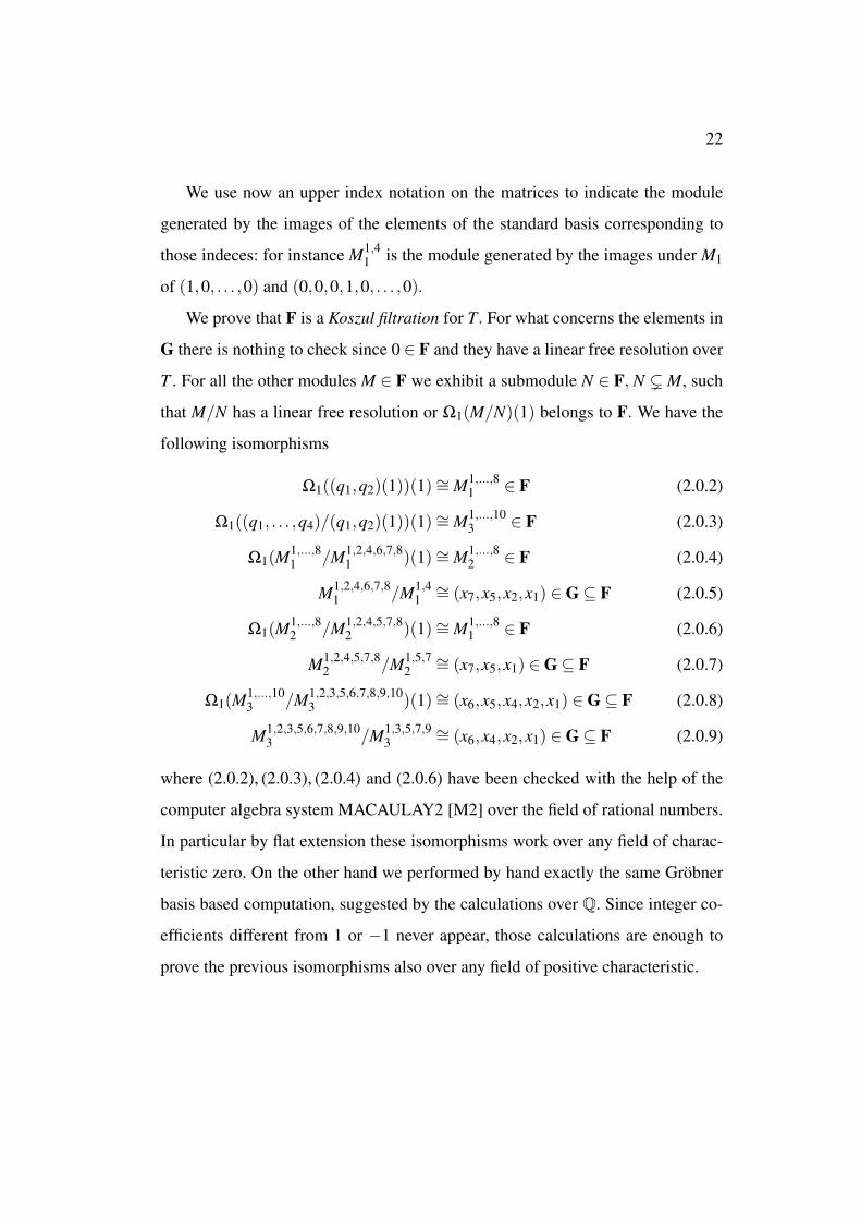
We use now an upper index notation on the matrices to indicate the module

generated by the images of the elements of the standard basis corresponding to

those indeces: for instance M1,41 is the module generated by the images under M1

of (1,0, . . . ,0) and (0,0,0,1,0, . . . ,0).

We prove that F is a Koszul filtration for T. For what concerns the elements in

G there is nothing to check since 0 ∈ F and they have a linear free resolution over

T . For all the other modules M ∈ F we exhibit a submodule N ∈ F, N ( M, such

that M/N has a linear free resolution or Ω1(M/N)(1) belongs to F. We have the

following isomorphisms

Ω1((q1,q2)(1))(1)∼= M1,...,81 ∈ F (2.0.2)

Ω1((q1, . . . ,q4)/(q1,q2)(1))(1)∼= M1,...,103 ∈ F (2.0.3)

Ω1(M1,...,81 /M1,2,4,6,7,8

1 )(1)∼= M1,...,82 ∈ F (2.0.4)

M1,2,4,6,7,81 /M1,4

1∼= (x7,x5,x2,x1) ∈G⊆ F (2.0.5)

Ω1(M1,...,82 /M1,2,4,5,7,8

2 )(1)∼= M1,...,81 ∈ F (2.0.6)

M1,2,4,5,7,82 /M1,5,7

2∼= (x7,x5,x1) ∈G⊆ F (2.0.7)

Ω1(M1,...,103 /M1,2,3,5,6,7,8,9,10

3 )(1)∼= (x6,x5,x4,x2,x1) ∈G⊆ F (2.0.8)

M1,2,3,5,6,7,8,9,103 /M1,3,5,7,9

3∼= (x6,x4,x2,x1) ∈G⊆ F (2.0.9)

where (2.0.2), (2.0.3), (2.0.4) and (2.0.6) have been checked with the help of the

computer algebra system MACAULAY2 [M2] over the field of rational numbers.

In particular by flat extension these isomorphisms work over any field of charac-

teristic zero. On the other hand we performed by hand exactly the same Grobner

basis based computation, suggested by the calculations over Q. Since integer co-

efficients different from 1 or −1 never appear, those calculations are enough to

prove the previous isomorphisms also over any field of positive characteristic.

23

In (2.0.5) and (2.0.7) the modules M1,41 and M1,5,7

2 are clearly isomorphic to

(x7,x4) ∈ G ⊆ F and to (x7,x2,x1) ∈ G ⊆ F respectively. Similarly in (2.0.9) the

module M1,3,5,7,93 is isomorphic to (x6,x5,x4,x2,x1) which belongs to G⊆ F. This

show that F is a Koszul filtration and, as we said before, by Proposition 1.1.3 the

ideal (q1 . . . ,q4)(1) has a linear free resolution over T. Thus the claim is proved

and so is the theorem.

Chapter 3

Castelnuovo-Mumford regularity and Hyperplane sections

This chapter gives an introduction to the methods of computing the Castelnuovo-

Mumford regularity using hyperplane sections. First, we treat the definitions and

some basic properties of the regularity. Second, we explore some equivalent def-

initions of regularity obtained by the use of generic hyperplane sections. Our

focus is on a well-known criterion of Bayer and Stillman (see [BS]) for detect-

ing regularity: we will show how to use a single approach to derive this one and

other similar criteria. More precisely, we deduce from a formula of Serre that

the Castelnuovo-Mumford regularity can be described in terms of the postulation

numbers of filter regular hyperplane restrictions, where the postulation number

α(M) of a module M is defined as the largest nonnegative integer for which the

Hilbert function of M is not equal to the corresponding Hilbert polynomial.

Finally, we draw a parallel comparison between Bayer-Stillman and our crite-

rion. In particular, we obtain, for both of them, a result that is very closely related

to the Crystallization Principle for generic initial ideals.

25

3.1 Castelnuovo-Mumford regularity

We recall the definition of the Castelnuovo-Mumford regularity, and we refer the

reader to [EG], [Ei] and [BS] for further details on the subject.

Definition 3.1.1. Let M be a finitely generated graded R-module and let βi j(M)

denote the graded Betti numbers of M (i.e. the numbers dimK Tori(M,K) j). The

Castelnuovo-Mumford regularity reg(M) of M is

maxi, j j− i|βi j(M) 6= 0.

Remember also this equivalent definition of regularity in terms of the local co-

homology modules of M, which we shall use later. Since the graded local coho-

mology modules H im(M) with support in the maximal graded ideal m of R are Ar-

tinian, one defines Max(H im(M)) as the maximum integer k such that H i

m(M)k 6= 0.

Then

reg(M) = maxiMax(H i

m(M))+ i.

Finally, a finitely generated R-module M is said to be m-regular for some integer

m if and only if reg(M)≤ m.

Example 3.1.2. Let R = K[X1, . . . ,Xn] be a polynomial ring and I = ( f1, . . . , fr) a

homogeneous ideal generated by a regular sequence of forms of degree d1, . . . ,dr.

Looking at the Koszul complex given by f1, . . . , fr we note that the maximum of

j− i|βi j(R/I) 6= 0 is obtained at βra(R/I) where a = ∑r1 di. Therefore reg(R/I)

is (∑r1 di)− r = ∑

r1(di−1).

3.1.1 Partial Regularities and short exact sequences

It is useful to recall the behavior of the regularity with respect to short exact se-

quences. In order to get some more precise statements, that we will need in the

26

next sections, we want to introduce some partial Castelnuovo-Mumford regularity.

We define partial Castelnuovo-Mumford regularities for M with respect to a

set of indices X ⊆ 0, . . . ,n as following:

Definition 3.1.3. Given a set of indices X ⊆ 0, . . . ,n and a finitely generated

graded R-module M we set regX (M) to be:

regX (M) = maxi∈XMax(H i

m(M))+ i.

We say that M is m-regular with respect to X (i.e m-regX ) if regX (M)≤m. Simi-

larly we set regX (M) to be:

regX (M) = maxi∈XMax(Tori(M,K))− i,

and we say that M is m-regX if regX (M)≤ m.

Remark 3.1.4. Note that when X = 0, . . . ,n the m-regX agrees with m-regularity

in the sense of Castelnuovo-Mumford. We notice that, from the Grothendieck van-

ishing theorem, all the local cohomology modules are zero for indexes bigger

than n. On the other hand since the projective dimension of M is always bounded

by n also the modules Tori(M,K) are zero for indexes bigger than n, therefore

it makes sense to use the following notation: given a ∈ Z we set X + a to be

i+a|i ∈ X ⋂0, . . . ,n.

The next lemma describes the behavior of the regularity with respect to X for

exact sequences.

Lemma 3.1.5. Given an exact sequence of finitely generated graded R-module,

0 −−−→ M −−−→ N −−−→ P −−−→ 0,

we have:

27

(1) If M and P are m-regX so is N.

(2) If N is m-regX and P is (m−1)-regX−1 then M is m-regX .

(3) If M is (m+1)-regX+1 and N is m-regX then P is m-regX .

Similarly:

(a) If M and P are m-regX so is N.

(b) If N is m-regX and P is (m+1)-regX+1 then M is m-regX .

(c) If M is (m−1)-regX−1 and N is m-regX then P is m-regX .

Proof. The proof of the first three facts follows from the long exact sequence

of local cohomology modules. The remaining three statement can be proved by

looking at the long exact sequence of Tor’s.

3.1.2 Regularity of a filter regular hyperplane section

Using the definition of Castelnuovo-Mumford regularity that involves the local

cohomology modules, it is easy to see that the regularity behaves quite well under

certain hyperplane section. These sections, called filter regular, are the ones that

avoid all the associated primes different from the homogenous maximal ideal.

More precisely:

Definition 3.1.6. A homogeneous element l ∈ R of degree D is filter regular on

a graded R-module M if the multiplication map l : Mi−D→Mi is injective for all

i 0. A sequence l1, . . . , lr of homogeneous elements of R is called a filter regular

sequence on M if li is filter regular on M/(l1, . . . , li−1)M for i = 1, . . . ,m.

28

Remark 3.1.7. Since H0m(M) = u ∈ M | mku = 0 for some k, then l is filter

regular on M if an only if l is a non-zerodivisor on M/H0m(M).

Remark 3.1.8. The regularity of a module does not change by extending the field

K, therefore we can assume K to be infinite. This will ensure the existence of filter

regular elements (for example any generic element is filter regular).

Proposition 3.1.9. Let M be a finitely generated graded R-module and l ∈ R a

filter regular element on M of degree D. Then for any set of indices X ⊆ 0, . . . ,n

we have:

(1) regX+1(M)≤ regX∪(X+1)(M/lM)−D+1

(2) regX (M/lM)−D+1≤ regX∪(X+1)(M).

Proof. Consider the short exact sequence

0 −−−→ (M/0 :M l)(−d) ·l−−−→ M −−−→ M/lM −−−→ 0.

Note that, since l is filter regular on M, H im((M/0 :M l)(−D))∼= H i

m(M)(−D) for

all i > 0. Looking at the long exact sequence of local cohomology modules, we

have

. . . −−−→ H im(M) −−−→ H i

m(M/lM) −−−→ H i+1m (M)(−D) −−−→

−−−→ H i+1m (M) −−−→ H i+1

m (M/lM) −−−→ . . .

for all i≥ 0.

Let j > regX∪(X+1)(M/lM)−D+1 and i∈ X . Consider the exact sequence of

K-vector spaces given by the graded pieces of degree j− i+D−1 of the previous

sequence. Because of the choice of j, we have

H im(M/lM) j−i+D−1 = H i+1

m (M/lM) j−i+D−1 = 0.

29

Therefore, H i+1m (M)(−D) j−i+D−1 ∼= H i+1

m (M) j−i+D−1, that is H i+1m (M) j−i−1 ∼=

H i+1m (M) j−i+D−1. An induction shows that H i+1

m (M) j−i−1 ∼= H i+1m (M) j−i+sD−1

for any s > 0. Since H i+1m (M) is Artinian, we obtain that H i+1

m (M) j−i−1 = 0 for

all i ∈ X , which implies part (1).

We prove now part (2). Take j > regX∪(X+1)(M) +D− 1 and i ∈ X . From

the choice of j, we have H im(M) j−i = H i+1

m (M)(−D) j−i = 0 for any i ∈ X . In

particular looking at the ( j− i)th graded component of the long exact sequence of

local cohomology modules we get H im(M/lM) j−i = 0 for all i ∈ X , which implies

part (2).

Proposition 3.1.9 has the following corollary:

Corollary 3.1.10. Given a finitely generated graded R-module M and a filter reg-

ular element l of degree D we have:

reg(M/H0m(M))≤ reg(M/lM)−D+1.

Proof. Set X = 0, . . . ,n and note that reg(M/H0m(M)) = regX+1(M). The con-

clusion follows from Proposition 3.1.9 (1).

3.2 Equivalent definitions of regularity using hyperplane sections

As we said in the introduction of this chapter, our main goal is to obtain results

relating regularity and invariants of hyperplane sections. The first example of such

a result is another corollary of Proposition 3.1.9.

Corollary 3.2.1 ([CH] Proposition 1.2). Given a finitely generated graded R-

module M and a filter regular element l of degree D we have:

reg(M) = maxMaxH0m(M), reg(M/lM)−D+1. (3.2.1)

30

Proof. Let X = 0, . . . ,n, and note that reg(M) = maxreg0(M), regX+1(M).

Clearly reg0(M) = MaxH0m(M).

From Proposition 3.1.9 (1) we have regX+1(M)≤ regX∪(X+1)(M/lM)−D+1 =

reg(M/lM)−D+1. Thus we get reg(M)≤maxMaxH0m(M), reg(M/lM)−D+

1. On the other hand, MaxH0m(M) ≤ reg(M) and, by Proposition 3.1.9 (1), we

have regX (M/lM)−D+1≤ regX∪(X+1)(M) = reg(M).

Note that for a finitely generated graded module N of dimension zero H0m(N)=

N, therefore reg(N) = MaxH0m(N). An easy induction on the formula 3.2.1 shows

the known fact:

Theorem 3.2.2 ([CH] Proposition 1.2). Let M be a finitely generated graded R-

module of dimension d. Then reg(M) = maxi∈0,...,dMaxH0m(M/(l1, . . . , li)M)−

∑ij=1(D j−1)) where l1, . . . , ld is a filter regular sequence of degrees D1, . . . ,Dd.

Theorem 3.2.2 can be found in [Gr1] (see Theorem 2.30 (5),(6)) under the

more restricted assumptions that the field K has characteristic zero and the li’s are

generic linear forms.

3.2.1 Regularity and Postulation Numbers

We prove how the Castelnuovo-Mumford regularity of M, with dimM = d, can

be obtained as the maximum of all the postulations numbers of d filter regular

hyperplane sections. More precisely we want to obtain an analogue of Theorem

3.2.2 where the function MaxH0m(N) is replaced by the postulation number α(N).

Below we will denote by HM(i) the value at i of the Hilbert function of M

(i.e HM(i) = dimK Mi), and with PM(i) the corresponding Hilbert polynomial. It is

well-known that PM(i) agrees with HM(i) for i 0. We recall also that, by a the-

orem of Hilbert, the Hilbert series (i.e. the formal series defined as ∑i∈ZHM(i)Zi)

31

has a rational expression h(Z)(1−Z)d where h(Z)∈Z[Z,1/Z]. When a graded R-module

M has dimension 0, we will denote by maxM the degree of its highest nonzero

graded component.

Definition 3.2.3. Let M be a finitely generated graded R-module with Hilbert

series h(Z)(1−Z)d . Let h(Z) = ∑

bi=a ciZi with cb 6= 0. We set the postulation number of

M to be α(M) = b−d.

Remark 3.2.4. It is a well-known fact that the postulation number of M is equal to

the highest degree i for which the Hilbert function differs from the Hilbert poly-

nomial (i.e HM(i)−PM(i) 6= 0). For a proof see for example Proposition 4.1.12 in

[BH]. The following formula of Serre (see [BH] Theorem 4.4.3 for a proof)

HM(i)−PM(i) =d

∑j=0

(−1) j dimK H jm(M)i for all i ∈ Z, (3.2.2)

shows how the postulation number of M can be defined in terms of the local co-

homology modules H im(M).

Theorem 3.2.5. Let M be a finitely generated graded R-module with dim(M) = d.

Then

reg(M) = maxi∈0,...,d

α(M/(l1, . . . , li)M)−i

∑j=1

(D j−1))

where l1, . . . , ld is a filter regular sequence of degrees D1, . . . ,Dd.

Proof. By definition, given any finitely generated graded R-module N and any

i > reg(N), we have H jm(N)i− j = 0. In particular H j

m(N)i = 0, hence from (3.2.2)

it is clear that reg(N)≥ α(N) for every N.

By Corollary 3.2.1, reg(M)≥ reg(M/lM)−deg l +1 for any filter regular el-

ement l, so we have:

reg(M)≥ maxi∈0,...,d

α(M/(l1, . . . , li)M)−i

∑j=1

(D j−1)).

32

We need to prove the reverse inequality. We do an induction on the dimension of

M. If dimM = 0, then reg(M) = MaxH0m(M) which equals to α(M), by (3.2.2).

Assume d > 0. By induction hypothesis we get:

reg(M/l1M) = maxi∈1,...,d

α(M/(l1, l2, . . . , li)M)−i

∑j=2

(D j−1)).

Consequently, setting a = maxi∈0,...,dα(M/(l1, . . . , li)M)−∑ij=1(D j−1)) we

have:

reg(M/l1M)−D1 +1≤ a.

Because of Corollary 3.2.1 we still need to prove that MaxH0m(M)≤ a. By Corol-

lary 3.1.10, since H jm(M)∼= H j

m(M/H0m(M)) for all j > 0, we have H j

m(M)>a− j =

0 for all j > 0. In particular, for any b > a, H jm(M)b = 0 for all j > 0. Hence, by

(3.2.2) we deduce HM(b)−PM(b) = dimK H0m(M)b. But a ≥ α(M) so HM(b)−

PM(b) = 0 for all b > a≥ α(M). Therefore, maxH0m(M)≤ a.

An interesting corollary of the Theorem 3.2.5 is the following:

Corollary 3.2.6. Let M be a finitely generated graded R-module. Let dimM = d,

and let l1, . . . , ld be a filter regular sequence on M of degree D1, . . . ,Dd. Then the

number

maxi∈0,...,d

α(M/(l1, . . . , li)M)−i

∑j=1

(D j−1))

is independent of the choice of the filter regular sequence and of its degrees.

3.2.2 Regularity and hyperplane sections: a general approach

We want to study the general properties of the functions Max(H0m( )) and α( ) on

which Theorem 3.2.2, Theorem 3.2.5 and Corollary 3.2.6 rely.

33

From Remark 3.2.4, the number α(M) is the highest integer i for which the

function φ defined as

φ(i,M0,M1,M2, . . . ,Mn) :=n

∑j=0

(−1) j dimK(M j)i

is not zero at (i,H0m(M),H1

m(M), . . . ,Hnm(M)).

On the other hand Max(H0m(M)) is trivially the highest integer i for which the

function θ defined as

θ(i,M0,M1,M2, . . . ,Mn) := dimK(M0)i

is not zero at (i,H0m(M),H1

m(M), . . . ,Hnm(M)).

It is possible to replace for φ and θ any other function ψ such that, whenever

(M j)>i− j = 0 for all j > 0, we have:

ψ(i,M0,M1,M2, . . . ,Mn) 6= 0 if and only if (M0)i 6= 0. (3.2.3)

For example, instead of α( ) or MaxH0m( ) we could use the function β( ) defined

as:

β(M) = supi | ψ(i,H0m(M),H1

m(M), . . . ,Hnm(M)) 6= 0.

The following result holds:

Theorem 3.2.7. For such a β defined as above we have:

reg(M) = maxi∈0,...,d

β(M/(l1, . . . , li)M)−i

∑j=1

(D j−1))

where M is a finitely generated graded module of dimension d and l1, . . . , ld is a

filter regular sequence of degrees D1, . . . ,Dd.

34

Remark 3.2.8. If two functions ψ1 and ψ2 satisfying the above property (3.2.3)

then also minψ1,ψ2 and maxψ1,ψ2 satisfy (3.2.3). Moreover if we call β1

and β2 the corresponding functions associated with ψ1,ψ2 then minψ1,ψ2 and

maxψ1,ψ2 are associated with minβ1,β2 and maxβ1,β2. This observation

allows us to obtain the following result of independence.

Theorem 3.2.9. Let β1, . . . ,βd be defined as above and let l1, . . . , ld be a filter

regular sequence of forms of degrees D1, . . . ,Dd over a module M of dimension d.

Then the number

maxi∈0,...,d

βi(M/(l1, . . . , li)M)−i

∑j=1

(D j−1)) (3.2.4)

is equal to the regularity of M and therefore does not depend on the filter regular

sequence chosen not on the functions βi.

Proof. Define the function γ1 to be minβi and γ2 to be maxβi. Thanks to

Remark 3.2.8 we can apply Theorem 3.2.7 and get:

reg(M) = maxi∈0,...,d

γ1(M/(l1, . . . , li)M)−i

∑j=1

(D j−1)) ≤

maxi∈0,...,d

βi(M/(l1, . . . , li)M)−i

∑j=1

(D j−1)) ≤

maxi∈0,...,d

γ2(M/(l1, . . . , li)M)−i

∑j=1

(D j−1))= reg(M).

Therefore the middle term is equal to reg(M).

3.2.3 Bayer and Stillman criterion for detecting regularity and some similar

further criteria

In this section we discus the Bayer and Stillman criterion for detecting regularity.

Below we will focus on modules as our main object of study: working with ideals

35

does not give a significant simplification to the treatment. The reader can refer to

Bayer and Stillman’s original paper [BS] for the ideal-theoretic discussion. This

criterion, as outlined in [BS], is a key point for the introduction and the study

of generic initial ideals. Similarly, we will explore consequences of criteria for

regularity in the next chapters: bounds for regularity and the structure of Gins rely

significantly on those criteria.

Consider a finitely generated module M with a minimal presentation as M =

F/N, where F is a free module (maybe with some shifts: i.e. F =⊕R(−i)bi) and

N is a nonzero submodule. The basic question behind these criteria is the follow-

ing: Assuming the knowledge of the highest degree of a minimal homogeneous

generator of N (i.e. maxTor1(M,K) or reg1(M)+1 ), how can one improve the

formulas in Theorem 3.2.1, 3.2.5, 3.2.7, and 3.2.9?

Concerning Theorem 3.2.1 an answer is given by the following criterion of

Bayer and Stillman:

Theorem 3.2.10 (Bayer and Stillman criterion). Let M be a finitely generated

graded module. Let f be a homogenous polynomial such that (0 :M f )a+1 = 0,

for some a ≥ maxreg(M/ f M)− (deg( f )− 1), reg1(M). Then (0 :M f )≥a+1

is zero (if M has positive dimension f is therefore filter regular) and moreover

reg(M)≤ a.

Proof. Write M minimally as F/N where F is a free module. First we want to

show that the degree of the minimal generators of N and N :F f are bounded by

a+ 1. This is equivalent to showing reg1(M) ≤ a and reg1(M/(0 :M f ) ≤ a.

While the first inequality is by assumption, the second follows from the short exact

sequence

0 −−−→ (M/0 :M f )(−deg( f ))· f−−−→ M −−−→ M/ f M −−−→ 0.

36

In fact, using Lemma 3.1.5 we have:

reg1(M/0 :M f )≤maxreg1(M), reg2(M/ f M)+1−deg( f )

which is bounded by a. Now, because (0 :M f ) = (N :F f )/N, the fact that this

module is zero in a degree a+1, greater or equal than the degree of the minimal

generators of N :F f and N, implies ((N :F f )/N)≥a = 0. In particular (0 :M f ) has

finite length and, therefore, if the dimension of M is positive, f is filter regular.

We still have to show that reg(M) ≤ a. Note that since (0 :M f )≥a+1 = 0 then

(0 :M f ∞)≥a+1 = 0. This implies (0 :M f ∞) = H0m(M) and, in particular, it gives

maxH0m(M) ≤ a, that is enough for the dimension zero case. If the dimension of

M is positive we know that f is filter regular and by Corollary 3.2.1 we have

reg(M)≤ maxH0m(M), reg(M/ f M)−deg( f )+1,

which is less than or equal to a.

Remark 3.2.11. Note that in the proof of Theorem 3.2.10, in order to obtain

(0 :M f )≥a+1 =H0m(M)≥a+1 = 0 it was enough to have a≥maxreg2(M/ f M)−

(deg( f )−1), reg1(M).

Corollary 3.2.12. Let M be a finitely generated graded module and let f be a

filter regular element. Set c = maxreg(M/ f M)− (deg( f )−1), reg1M. Then

reg(M) = mina|(0 :M f )a+1 = 0 and a≥ c

= mina−1|H0m(M)a+1 = 0 and a≥ c.

Proof. By the previous Theorem the first term is smaller than or equal to the

second. On the other hand, (0 :M f ) ⊆ (0 :M f ∞) = H0m(M), therefore, the sec-

ond term is smaller than or equal to the third. Corollary 3.2.1 gives reg(M) ≥

37

reg(M/ f M)− (D− 1) and, in particular, reg(M) ≥ c. Since H0m(M)reg(M)+1 is

zero, we have that

reg(M) ∈ a|(0 :M f )a+1 = 0 and a≥ c

which proves that the third term is smaller than or equal to the first.

Remark 3.2.13. Using the notation of the previous section we will consider now a

function ψ satisfying condition (3.2.3). With an abuse of notation we will denote

the function ψ(i,H0m(M),H1

m(M), . . . ,Hnm(M)) by ψ(i,M). Recall that the differ-

ence between the Hilbert polynomial and the Hilbert function of a module is one

of such a ψ.

We can state then two variations of Theorem 3.2.10 and Corollary 3.2.12.

Proposition 3.2.14. Let M be a finitely generated graded module and let ψ be a

function defined as above. Let f be a homogenous filter regular polynomial such

that ψ(a+1,M) = 0, for some a≥maxreg(M/ f M)− (deg( f )−1), reg1(M).

Then ψ(i,M) = 0 for all i≥ a+1 and moreover reg(M)≤ a.

Proof. In order to prove that reg(M)≤ a it is enough to show that the hypotheses

of Theorem 3.2.10 are satisfied. By part (1) of Proposition 3.1.9 we know that

reg1,...,n(M) ≤ reg(M/ f M)− (deg( f )− 1) which is bounded by a. Therefore,

H im(M)a+1−i = 0 and by the properties of ψ we have that ψ(a+ 1,M) = 0. This

implies H0m(M)a+1 = 0, which gives (0 :M f )a+1 = 0.

To prove that ψ(i,M)= 0 for all i≥ a+1 it is enough to observe that ψ(i,M)=

0 if and only if H0m(M)i = 0. This condition is satisfied because we know that

reg(M)≤ a < i, and we can use Corollary 3.2.12.

38

Corollary 3.2.15. Under the same assumptions of Corollary 3.2.12 we have:

reg(M) = mina|ψ(a+1,M) = 0 and a≥ c. (3.2.5)

Proof. We know that for a≥ c the function ψ(a+1,M) is equal to zero if and only

if H0m(M)a+1 = 0. Therefore the result follows directly from Corollary 3.2.12.

3.2.4 Crystallization principle

In this section we want to underline one immediate consequences of Corollary

3.2.15. The choice of the title will be clarified later when we will study some

applications of the result of this section. In particular we will give a proof of the

crystallization principle for generic initial ideals in characteristic zero, by using

this result. Below ψ will denote a function defined in Remark 3.2.13.

The following Lemma is an immediate and direct consequence of Corollary

3.2.12 and Corollary 3.2.15.

Lemma 3.2.16. Let M be a finitely generated graded module and let f be a fil-

ter regular form. Let c ≥ maxreg1M, reg(M/ f M)− (deg( f )− 1) Then the

following sets of indexes are the same:

(1) S1 = j|(0M : f ) j 6= 0, and j ≥ c

(2) S2 = j|H0m(M) j 6= 0 and j ≥ c

(3) S3 = j|ψ( j,M) 6= 0 and j ≥ c

(4) S4 = j|c≤ j ≤ reg(M).

Proof. As we said above the proof follows from Corollary 3.2.12 which shows

S1 = S2 = S4, and from Corollary 3.2.15 which gives S3 = S4.

39

Proposition 3.2.17 (Crystallization Principle). Let M be a finitely generated graded

module over K[x1, . . . ,xn] and let l1, . . . , ln be a filter regular sequence of linear lin-

early independent over K. Let N0 = M, Ni = M/(l1, . . . , li)M and for i > 0 define

ci = maxreg1(M), reg(Ni). Then the following sets of indexes are the same:

(1) S1 = ∪n−1i=0 j|(0Ni : li+1) j 6= 0, and j ≥ ci+1

(2) S2 = ∪n−1i=0 j|H0

m(Ni) j 6= 0 and j ≥ ci+1

(3) S3 = ∪n−1i=0 j|ψ( j,Ni) 6= 0 and j ≥ ci+1

(4) S4 = j| reg1(M)≤ j ≤ reg(M).

Proof. First note that reg1(M) ≥ reg1(N1) ≥ . . . ,≥ reg1(Nn) = 0 moreover

each Ni is a module over a polynomial ring in n− i variables.

Define S1,i = j|(0Ni : li+1) j 6= 0, and j ≥ ci+1 for i = 0, . . . ,n−1, and similarly

define S2,i and S3,i. Set S4,i to be j|ci+1 ≤ j ≤ reg(Ni). To conclude the proof, it

is enough to show the following claim:

Claim 3. For any i = 0, . . . ,d−1 we have S1,i = S2,i = S3,i = S4,i.

Which follows from Lemma 3.2.16 applied to Ni and ci+1.

Remark 3.2.18. Following the same idea as in the proof of Theorem 3.2.9, we

could substitute the third set above for a more general one:

∪n−1i=0 j|ψi( j,Ni) 6= 0 and j ≥ ci+1,

where ψi - exactly as ψ - are functions defined in Remark 3.2.13.

Chapter 4

Weakly Stable Ideals and Castelnuovo-Mumford Regularity

This chapter is devoted to the study of a special kind of monomial ideals called

weakly stable ideals (see Definition 4.1.3). The notion has been introduced by

Enrico Sbarra and the author in [CS] in order to have a combinatorial property

satisfied both by strongly stable ideals and p-Borel ideals. In particular in [CS] we

use weakly stable ideals to reproduce an argument of Giusti to bound uniformly,

in characteristic zero, the Castelnuovo-Mumford regularity of all the ideals gener-

ated at most in degree d. We refer to the next chapter for the proofs of the bounds

in [CS], in particular we show how it is possible to use weakly stable ideals to

give a different proof of these bounds.

It is well known that the regularity of a stable ideal I is equal to the highest

degree of a minimal generator of I. This fact can be deduced, for example, by

looking at the Eliahou-Kervaire resolution of I, see [EK]. On the other hand in the

literature there is no equivalent formula for p-Borel ideals, and the only known

result, which was conjectured by Pardue and recently proved by J.Herzog and

D.Popescu [HP], is a quite complicated formula for the special case of p-Borel

principal ideals.

Later we show how to extend the formula for the regularity of stable ideals to

41

weakly stable ideals. We will prove:

Theorem 4.1.10. Let I ⊂ K[x1 . . . ,xn] be a weakly stable ideal minimally gener-

ated by the monomials u1, . . . ,ur. Assume that u1 > u2 > · · · > ur with respect to

the reverse lexicographic order (note that it is not the degree revlex). Then

reg(I) = maxdegui +C(ui) (A)

where C(ui) is set to be the highest degree of a monomial v in K[X1, . . . ,X j] such

that vui 6∈ (u1, . . . ,ui−1) and X j+1 is the last variable dividing ui.

It will follow easily that when I is strongly stable, the correction term C(ui) is

zero for all i.

In the first section we give the definition of weakly stable ideals and we show

that this combinatorial notion is equivalent to saying that all the primes associated

to such ideals are generated by lex-segments. This property allows us to make use

of the Bayer and Stillman criterion for detecting regularity, and prove that their

regularity does not depend on the characteristic of the base field. On the other

hand, we give an example of a weakly stable ideal for which the Betti numbers

depend on char(K).

In the second section we prove the formula (A) for the Castelnuovo-Mumford

regularity that was mentioned above.

4.1 General properties of Weakly Stable ideals

Strongly stable ideals, stable ideals and p-Borel ideals play an important role in

those areas of Commutative Algebra and Algebraic Geometry where certain ho-

mological invariants, for example projective dimension, Castelnuovo-Mumford

42

regularity and extremal Betti numbers, can be computed by combinatorial prop-

erties of the generic initial ideal. Generic initial ideals ideals are strongly stable

(and in particular stable) when charK = 0 and they are p-Borel if charK = p > 0.

We recall briefly those two notions (see [Pa1] for further details).

Notation 4.1.1. Given a monomial ideal I we define G(I) to be the set of its mini-

mal monomial generators. Given a monomial u we denote maxi such that Xi | u

by m(u) and the value max j such that X ji | u by |u|i. These notion can be nat-

urally extended to a monomial ideal by setting m(I) = maxm(u) with u ∈ G(I)

and |I|i = max|u|i with u ∈ G(I).

A monomial ideal I is strongly stable if for all u ∈ I, whenever Xi | u thenX juXi∈ I, for every j < i.

The wider class of stable ideals is defined by the following weaker exchange

condition on the variables of the monomials: an ideal I is stable if for every mono-

mial u ∈ I, X juXm(u)∈ I, for every j < m(u).

Example 4.1.2. In K[X ,Y,Z] the smallest stable ideal containing XY Z is I =

(X3,X2Y,XY 2,XY Z), which is not strongly stable since X2Z 6∈ I.

Let p be a prime number. Given two integers a and b, we write their p-adic

expansion as a = ∑i ai pi and b = ∑i bi pi respectively. One defines a partial order

≤p by saying that a≤p b if and only if ai ≤ bi for all i.

An ideal I is said to be p-Borel if for every monomial u∈ I, if b is the maximum

integer such that Xbi |u, then

Xaj u

Xai∈ I, for every i < j and a≤p b.

Notation. Given two monomial u and v, we will denote the monomial generator

of the ideal (u) : v∞ simply by u : v∞.

43

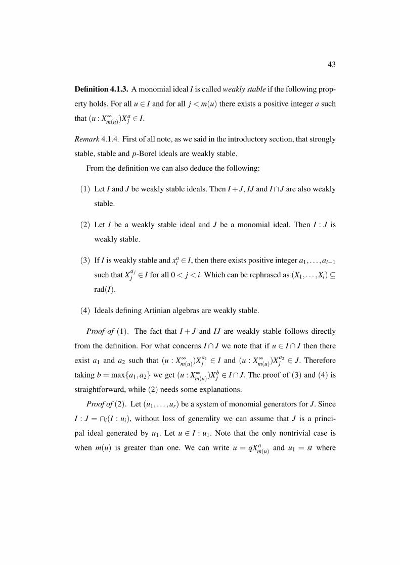
Definition 4.1.3. A monomial ideal I is called weakly stable if the following prop-

erty holds. For all u ∈ I and for all j < m(u) there exists a positive integer a such

that (u : X∞

m(u))Xaj ∈ I.

Remark 4.1.4. First of all note, as we said in the introductory section, that strongly

stable, stable and p-Borel ideals are weakly stable.

From the definition we can also deduce the following:

(1) Let I and J be weakly stable ideals. Then I+J, IJ and I∩J are also weakly

stable.

(2) Let I be a weakly stable ideal and J be a monomial ideal. Then I : J is

weakly stable.

(3) If I is weakly stable and xai ∈ I, then there exists positive integer a1, . . . ,ai−1

such that Xa jj ∈ I for all 0 < j < i. Which can be rephrased as (X1, . . . ,Xi)⊆

rad(I).

(4) Ideals defining Artinian algebras are weakly stable.

Proof of (1). The fact that I + J and IJ are weakly stable follows directly

from the definition. For what concerns I ∩ J we note that if u ∈ I ∩ J then there

exist a1 and a2 such that (u : X∞

m(u))Xa1j ∈ I and (u : X∞

m(u))Xa2j ∈ J. Therefore

taking b = maxa1,a2 we get (u : X∞

m(u))Xbj ∈ I ∩ J. The proof of (3) and (4) is

straightforward, while (2) needs some explanations.

Proof of (2). Let (u1, . . . ,ur) be a system of monomial generators for J. Since

I : J = ∩i(I : ui), without loss of generality we can assume that J is a princi-

pal ideal generated by u1. Let u ∈ I : u1. Note that the only nontrivial case is

when m(u) is greater than one. We can write u = qXam(u) and u1 = st where

44

q,s ∈ K[X1, . . . ,Xm(u)−1] and t ∈ K[Xm(u), . . . ,Xn]. Since qsXam(u)t ∈ I, by apply-

ing several times the property of the weak stability, we obtain qsXbm(u) ∈ I for

some b. On the other hand m(qsXbm(u)) = m(u) and therefore, by weak stability,

for any positive integer j < m(u) there exists a c such that qsXcj ∈ I. In particular

u : X∞

m(u)Xcj = qXc

j belongs to I : s⊆ I : u1.

We show now how the weak stability is in fact equivalent to some other, less

combinatorial, properties.

Set R = K[X1, . . . ,Xn], and let I to be a homogeneous ideal. We recall that a

homogenous element l of degree d is said to be filter regular for R/I = S if the

multiplication by l from Sa to Sd+a is an injective map for a >> 0. This is equiv-

alent to say that l does not belong to any of the associated primes of I different

from the homogeneous maximal ideal. The elements l1, . . . , li form an filter regular

sequence if, for any j = 1, . . . , i, the form l j is regular for R/(l1, . . . , l j−1).

Proposition 4.1.5. Let I ⊆ R be a monomial ideal. Then the following properties

are equivalent.

i) The ideal I is weakly stable.

ii) Any P ∈ Ass(I) is a lex-segment ideal.

iii) The variables Xn,Xn−1, . . . ,X1 are an filter regular sequence for R/I.

Proof. The fact that weak stability implies ii) is an immediate consequence of

Remark 4.1.4. Let P be an associated prime of I, we can then write it as P = I : m

for some monomial m. By Remark 4.1.4 part (2) P is weakly stable. Let Xi be the

variable belonging to P having the greatest index, in particular, by Remark 4.1.4

part (3), (X1, . . . ,Xi)⊆ P. The other inclusion holds by the choice of Xi.

45

Assume now that ii) holds true. It is clear that Xn is a filter regular element.

In order to prove iii), by a decreasing induction, it is enough to show that Xn−1 is

filter regular for K[X1, . . . ,Xn−1]/(I∩K[X1, . . . ,Xn−1]). The result follows because

property ii) is satisfied by I∩K[X1, . . . ,Xn−1].

Assume now that iii) holds. Let u be monomial in I and set J to be I ∩

K[X1, . . . ,Xm(u)]. Since Xm(u) is filter regular in K[X1, . . . ,Xm(u)]/J, the module

(J : X∞

m(u))/J has finite length and therefore for any positive i less than m(u) there

exists an ai for which (u : X∞

m(u))Xaii ∈ J ⊆ I.

A consequence of Proposition 4.1.5 is outlined by the next proposition, which

shows that the regularity and the projective dimension of a weakly stable ideal are

conbinatorial invariants. They are, therefore, independent of the characteristic of

the base field.

Proposition 4.1.6. Let J ⊂ Z[X1, . . . ,Xn] be a weakly stable monomial ideal and

let R = K[X1, . . . ,Xn]. Define the ideal I of R as I = JR. Then reg(I) and the pro-

jective dimension pd(I) depend only on J. Moreover pd(I) = m(I)−1.

Proof. Since I is weakly stable then Xn, . . . ,X1 is a filter regular sequence. Clearly

Xn, . . . ,Xm(I)+1 is a regular sequence for R/I and Xm(I) is a zerodivisor. Then by

Proposition 4.1.5 ii), we know that (X1, . . . ,Xm(I)) is associated to R/I and, there-

fore, depth(R/I) = n−m(I) and pd(I) = m(I)− 1 = m(J)− 1. To complete the

proof we show that reg(R/I), which is reg(I)−1, depends only on J. If n = 1 the

result is clear, moreover reg1 R/I is also clearly independent of R since it is the

highest degree of a minimal monomial generator of J. We can then do an induction

on the number of variables. By using Corollary 3.2.12 we know that reg(R/I) =

mina|(0 :R/I Xn)a+1 = 0 and a ≥ maxreg1(R/I), reg(R/(I +(Xn)). Whether

46

(0 :R/I Xn) is zero in a certain degree is independent of R and, therefore, by induc-

tion, the above set is independent too.

Remark 4.1.7. In general the regularity and the projective dimension of a mono-

mial ideal depend on char(K). The well-known example to show this fact, ob-

tained from the triangulation of P2, is the following: Let R = K[X1,X2, . . . ,X6]

and let I = (X1X2X3,X1X2X4,X1X3X5,X2X4X5,X3X4X5,X2X3X6,X1X4X6,X3X4X6,

X1X5X6,X2X5X6). If char(K) = 0 then R/I has the following resolution:

0 −−−→ R6(−5) −−−→ R15(−4) −−−→ R10(−3) −−−→ R/I −−−→ 0.

Which gives reg(I) = 3 and pd(I) = 2. On the other hand, if char(K) = 2 we have

the following resolution:

0 −−−→ R(−6) −−−→ R6(−5)⊕

R(−6) −−−→ R15(−4) −−−→

R10(−3) −−−→ R/I −−−→ 0,

which provides reg(I) = 4 and pd(I) = 4.

Note that I is not a weakly stable ideal since it does not contain a pure power of

the variable X1.

Proposition 4.1.6 is refined by Theorem 4.1.10 which gives a precise value for

reg I. In particular, Theorem 4.1.10 gives a different proof that the regularity of a

weakly stable ideal does not depend on char(K). Notice that, on the other hand, it

is possible to construct examples of weakly stable ideals whose graded Betti num-

bers depends of char(K). Take an ideal I, for example the one of the triangulation

of P2, whose Betti numbers depend on char(K) and then add a power of the homo-

geneous maximal ideal greater than reg(I). This new ideal, say J, is weakly stable

because it gives and Artinian Algebra and has graded Betti numebers depending

on char(K).

47

Before proving Theorem 4.1.10 it is useful to give the following two Lemmas.

Lemma 4.1.8. Let I be a monomial ideal and let u1 > u2 > · · ·> ur be the minimal

monomial generators of I ordered revlex. Then m((u1 u2, . . . ,ui−1) : ui)< m(ui).

Proof. Set J = (u1 u2, . . . ,ui−1) : ui. It is clear that m(J) ≤ m(u1,u2, . . . ,ui−1) ≤

m(ui). Let v be a minimal generator of J for which m(v) = m(J). We know that

there exists a monomial w such that vui = wu j for some 1≤ j ≤ i−1; this forces

v > w. On the other hand, since v is a minimal generator of J, v and w have no

common nontrivial factor, and in particular we get that m(v)< m(w)≤m(wu j) =

m(vui). This gives m(v)< m(ui).

The next Lemma explains the real meaning of the correction terms C(ui) ap-

pearing in Theorem 4.1.10.

Lemma 4.1.9. Let I ⊂ K[X1 . . . ,Xn] be a weakly stable ideal, and let u1 > u2 >

· · · > ur be the minimal monomial generators of I, ordered in revlex. Let j be

m(ui)−1 and define C(ui) as the highest degree of a monomial v in K[X1, . . . ,X j]

such that vui 6∈ (u1, . . . ,ui−1). Then C(ui) = regR/J where J = ((u1, . . . ,ui−1) : ui).

Proof. By Lemma 4.1.8 we know that m(J)≤ m(ui)−1 = j. Hence Xn, . . . ,X j+1

is a regular sequence for R/J, so regR/J = regR/(J + (Xn, . . . ,X j+1)). On the

other hand, since the ideal (u1, . . . ,ui) is weakly stable, there exist a1, . . . ,a j such

that (ui : X∞j+1)X

all ∈ I, for l = 1 . . . , j. More precisely, since (ui : X∞

j+1)Xall < ui,

we get that (ui : X∞j+1)X

all ∈ (u1, . . . ,ui−1). In particular, (Xa1

1 , . . . ,Xa jj ) ⊆ (J +

(Xn, . . . ,X j+1)), and, therefore, R/(J +(Xn, . . . ,X j+1) Artinian. The Castelnuovo-

Mumford regularity of R/(J +(Xn, . . . ,X j+1) is equal to the degree of its highest

nonzero graded component, which is exactly the highest degree of a monomial v

in K[X1, . . . ,X j] such that vui 6∈ (u1, . . . ,ui−1)K[X1, . . . ,X j+1].

48

We can now prove the following:

Theorem 4.1.10. Let I ⊂ K[X1 . . . ,Xn] be a weakly stable ideal minimally gener-

ated by the monomials u1, . . . ,ur. Assume that u1 > u2 > · · · > ur with respect to

the reverse lexicographic order and let ji be m(ui)−1. Then

reg(I) = maxdegui +C(ui), (A)

where C(ui) is set to be the highest degree of a monomial v in K[X1, . . . ,X j] such

that vui 6∈ (u1, . . . ,ui−1).

Proof. Set α(I) = maxdegui +C(ui). If r = 1 the formula is clear. We can,

therefore, do an induction on the number of generators of I. From the following

short exact sequence:

0→ (u1, . . . ,ur−1)→ I→ ((u1, . . . ,ur−1) : ur)(−degur)→ 0,

we deduce reg(I)≤maxreg((u1, . . . ,ur−1), reg((u1, . . . ,ur−1) : ur)+degur. By

Lemma 4.1.9 reg((u1, . . . ,ur−1) : ur)+ degur is precisely degur +C(ur). By in-

duction we know that reg(u1, . . . ,ur−1) = α((u1, . . . ,ur−1)), and therefore

reg(I)≤maxα((u1, . . . ,ur−1)),degur +C(ur)= α(I).

Assume, by contradiction, that reg I < α(I). Let i be the lowest index for which J,

defined as J = I∩K[X1, . . . ,Xi], satisfies α(J) = α(I). Since Xn . . . ,Xi+1 is a filter

regular sequence for R/I we have that reg(J) = reg(I +(Xn . . . ,Xi+1))≤ reg(I)<

α(I) = α(J). By substituting I for J, without loss of generality, we can assume

that reg(I) < α(I) and α((I ∩K[X1, . . .Xn−1])) < α(I), moreover this inequality

implies that α(I) is obtained at some ul with m(ul) = n. Since reg(I) ≤ α(I)− 1

we know that H0m(R/I) = (I : m∞)/I = (I : Xn

∞)/I is zero in degree α(I)− 1.

49

In particular, ((I : Xn)/I)α(I)−1 = 0. On the other hand, there exists a monomial

v∈K[X1, . . . ,Xn−1] such that v 6∈ (u1, . . . ,ul−1) : ul and deg(vul) = α(I). Note that

since the ui’s are ordered reverse lexicographically m(ul) = n implies m(u j) = n

for all j≥ l, therefore v 6∈ I. The element vul/Xn shows that ((I : Xn)/I)α(I)−1 6= 0

which is a contradiction.

As a corollary we get the well-known fact that the regularity of a strongly

stable ideal is equal to the highest degree of a minimal monomial generator.

Corollary 4.1.11. Let I ⊂ K[X1 . . . ,Xn] be a strongly stable ideal minimally gen-

erated by the monomials u1, . . . ,ur. Then reg(I) = maxdegui.

Proof. We can assume that u1 > u2 > · · · > ur with respect to the reverse lex-

icographic order. By using Theorem 4.1.10 it is enough to show that the cor-

rection terms C(ui) are zero. Since (ui/Xm(ui))X j ∈ I for all j < i we know that

(X1, . . . ,Xm(ui)−1) ⊆ (u1, . . . ,ui−1) : ui. On the other hand, Lemma 4.1.8 gives

the other inclusion, so (u1, . . . ,ui−1) : ui = (X1, . . . ,Xm(ui)−1). This implies that

C(ui) = 0.

The use of weakly stable ideals for investigating the regularity of homoge-

neous ideals is made more clear by the following results.

Lemma 4.1.12. Let I ⊂ K[X1 . . . ,Xn] be a homogeneous ideal. Then Xn, . . . ,Xi is

a filter regular sequence for R/I if and only if it is a filter regular sequence for

R/ inrlex(I).

Proof. For all s, i ≤ s ≤ n, define Js as I + (Xn, . . .Xs) and Hs as (inrlex(I) +

(Xn, . . .Xs)). Since the term-order we are using is the reverse lexicographic or-

der we have inrlex(Js) = Hs. The sequence Xn, . . . ,Xi is a filter regular sequence

50

for R/I (resp. for R/ inrlex I) if and only if (Js−1 : Xs)/Js−1 (resp. (Hs−1 : Xs)/Hs−1)

has finite length for all i≤ s≤ n.

From the short exact sequences

0→ (Js−1 : Xs)/Js−1→ R/Js−1·Xs−→ R/Js−1→ R/Js→ 0

and

0→ (Hs−1 : Xs)/Hs−1→ R/Hs−1·Xs−→ R/Hs−1→ R/Hs→ 0

we deduce that (Js−1 : Xs)/Js−1 and (Hs−1 : Xs)/Hs−1 have the same length since

for any index i the Hilbert function of R/Ji and R/Hi are the same.

Remark 4.1.13. From the above proof we also deduce that (I : Xn)/I and (inrlex(I) :

Xn)/ inrlex(I) have the same Hilbert function.

Corollary 4.1.14. Let I ⊂ K[X1 . . . ,Xn] be a homogeneous ideal. Then Xn, . . . ,X1

is a filter regular sequence for R/I if and only if inrlex(I) is weakly stable.

Proof. The result follows immediately from Lemma 4.1.12 and the equivalence

given by Proposition 4.1.5.

Remark 4.1.15. In the above Corollary, since any nonzero homogeneous form is

filter regular over an Artinian ring, we can substitute Xn, . . .Xd for Xn, . . .X1, with

d = dimR/I.

The next Proposition is a slight extension of the well-know fact that the reg-

ularity and the projective dimension of an ideal are preserved by taking generic

initial ideal with respect to the reverse lexicographic order.

Proposition 4.1.16. Let I ⊂ K[X1 . . . ,Xn] be a homogeneous ideal. If inrlex(I) is

weakly stable, then reg(I) = reg(inrlex(I)) and pd(I) = pd(inrlex(I)).

51

Proof. The fact that the projective dimension is preserved is equivalent to say that

the depth is preserved. Assume that depth(R/I) = a, then since Xn, . . . ,X1 is a

filter regular sequence for R/I we get that Xn, . . . ,Xa is a regular sequence for R/I.

On the other hand the Hilbert functions of R/(I+(Xn, . . . ,Xa)) and R/(inrlex(I)+

(Xn, . . . ,Xa)) = R/ inrlex((I)+(Xn, . . . ,Xa)) are the same, therefore X1, . . . ,Xa is a

regular sequence also for R/ inrlex(I). If depth(R/ inrlex(I)) = b, we deduce that

Xn, . . . ,Xb is regular for R/ inrlex(I), and in the same way, we get depth(R/I)≥ b.

For what concerns the regularity we recall that for any ideal N and for any filter

regular sequence of linear forms ln . . . , l1 for R/N we have

reg(N) = maxMax(N +(ln, . . . , li−1) : li)/(N +(ln, . . . , li−1)

where Max(M) stands for the highest nonzero graded component of a finite length

module M. Keeping the same notation of Lemma 4.1.14, we see that its proof

shows that the Hilbert function of (Js−1 : Xs)/Js−1 and (Hs−1 : Xs)/Hs−1 are the

same. Therefore, by using the above formula, we get reg(I) = reg(inrlex(I)).

In the next section we present an example of a family of ideals with high reg-

ularity. This gives us the opportunity to show how to combine the use of Theorem

4.1.10 and Proposition 4.1.16.

4.2 Ideals with high Castelnuovo-Mumford regularity

Given an ideal I ⊆ K[X1, . . . ,Xn] generated by polynomials of degrees d1, . . . ,dr

we know that maxdi ≤ reg(I). In general, without any assumption on I, the

difference between the degree of the generators and the regularity of I can be very

large. The most famous example in the literature, showing this bad behavior, was

given by Mayr and Meyer in [MM]. This important example consists of a family

52

of ideals of quartics (a variation, due to Jee Koh, gives an ideal of quadrics),

depending on the number of variables of the ring. It is quite natural to ask whether

it is possible to construct examples of ideals with large regularity (with respect to

the degree of the generators) for a fixed polynomial ring. In this setting there is a

uniform bound for the regularity of all the ideals generated in a fixed degree, so

it makes more sense to ask for a family of ideals depending on the degree of the

generators.

The example we give in this section is an extremely simple one: it is given by

two monomial and a binomial of degree d in four variable. The computation of the

regularity for these ideals is obtained quite easily by the use of results concerning

weakly stable ideals.

Example 4.2.1. Let I = (Xd1 ,X

d2 ,X1Xd−1

3 −X2Xd−14 ) be a homogeneous ideal of

K[X1,X2,X3,X4] with d ≥ 2. Then reg(I) = d2−1.

Proof. First we show that:

inrlex(I) = (Xd1 ,X

d2 ,X1Xd−1

3 ,Xd−i1 (X2Xd−1

4 )i for i = 1, . . . ,d−1).

More generally we construct a Grobner basis for I as follow.

Set g1 = X1Xd−13 −X2Xd−1

4 , g2 = Xd2 ,g3 = Xd

1 and then define recursively

g3+i = g2+iXn−13 −g1Xd−i

1 (X2Xd−14 )i−1.

Note that g3+i = Xd−i1 (X2Xd−1

4 )i. By construction we have that all the g j’s be-

long to I, moreover all the S-pairs are reducible. Therefore the g j’s are a Grobner

basis for I. It is immediate to check, using the definition involving the exchange

property, that inrlex(I) is weakly stable. Therefore by Proposition 4.1.16 we know

53

that reg(I) = reg(inrlex(I)). By using Theorem 4.1.10 and by ordering the gener-

ators as Xd1 < Xd

2 < X1Xd3 −1 < Xd−1

1 (X2Xd−14 ) · · · < X1(X2Xd−1

4 )d−1 we have to

find the highest value for deg(u j)+C(u j) where u j is the jth minimal generator.

This maximum is obtained at the very last generator, i.e X1(X2Xd−14 )d−1. We have

that deg(X1(X2Xd−14 )d−1) = 1+d(d−1) and that C(X1(X2Xd−1

4 )d−1) is given, for

example, by Xd−23 . We obtain that reg(I) = 1+d(d−1)+d−2 = d2−1.

This example shows that even with a fixed number of variable and a fixed

number of generators for an ideal I (even with a fixed cardinality of the monomial

supports for the generator of the ideal) the Castelnuovo-Mumford regularity of

I could be much larger than the one corresponding to the complete intersection

case.

Remark 4.2.2. A possible generalization of the above example is given by the fol-

lowing ideals. Let R = K[X1, . . . ,Xr,Y1, . . . ,Yr] and set Id = (Xd1 ,Y

d1 )+(XiXd−1

i+1 −

YiY d−1i+1 )|1≤ i≤ n−1). Computational experiments seem to indicate that reg(Id),

as a function of d, is given by a polynomial P(d) of degree r.

Chapter 5

Uniform bounds for the Castelnuovo-Mumford regularity

In the literature we frequently find attempts bound the Castelnuovo-Mumford reg-

ularity and, in general, the expected results range quite widely, from the well-

behaved examples coming from the algebraic geometry, as suggested by the Ei-

senbud-Goto Conjecture [EG], to the worst case provided by the example of Mayr

and Meyer [MM].

In general, under quite unrestrictive assumptions, the regularity can be very

large. If one works with a homogeneous ideal I in a polynomial ring with n vari-

ables over a field K, a very natural question to ask is whether the regularity can be

bounded just by knowing the highest degree, say d, of a minimal homogeneous

generator.

If charK = 0, as observed in [BM] (Proposition 3.8), from the work of Giusti

[Gi] and Galligo [Ga1], [Ga2] one can derive

reg(I)≤ (2d)2n−2. (A)

On the other hand, in any characteristic, it has been proven by Bayer and

Mumford [BM], using cohomological methods, that

reg(I)≤ (2d)(n−1)!, (B)

55

but in the same paper it is asked whether (A) holds in general independently of

the characteristic.

This question was answered positively by the author and E.Sbarra in [CS]. The

main effort in extending the result to positive characteristic is that Giusti’s proof

utilizes the combinatorial structure of the generic initial ideal, in characteristic

zero, with respect to the reverse lexicographic order. More precisely a key point

in that proof is the following fact known as Crystallization Principle.

CP: Let I be a homogeneous ideal generated in degrees ≤ d. Assume also that

Ginrlex(I) has no generator in degree d +1. Then there are no generators of

Ginrlex(I) of degree higher than d ( [Gr1], Proposition 2.28).

Note that the Crystallization Principle, as stated above, only holds in characteristic

zero. Consider, for instance, the ideal (X2p,Y 2p) in K[X ,Y ] with charK = p 6= 2.

In this case Ginrlex(I) can be computed by observing that the ideal (X2p,Y 2p) is

the ideal generated by the images of X2 and Y 2 under the Frobenius map R→ R,

X → X p. In fact from the next result it follows that Ginrlex(I) = (X2p,X pY p,Y 3p).

Proposition 5.0.3. Let I be a homogeneous ideal of R = K[X1, . . . ,Xn]. Assume

charK = p and let F be the Frobenius map. Then, for any term order τ one has

Ginτ(F(I)) = F(Ginτ(I)).

Proof. Note that the computation of the initial ideal of F(I) can be performed in

K[X p1 , . . . ,X

pn ], i.e. the S-pairs of F(I) are just the p-th power of the S-pairs of

I, so that F(inτ(I)) = inτ(F(I)). This suffices, since by definition Ginτ(F(I)) =

inτ(g(F(I))) = inτ(F(g(I))), where g is a generic change of coordinates.

56

In [CS] we replaced the use of the crystallization principle by using the Bayer

and Stillman criterion for detecting regularity. A posteriori this substitution seems

quite natural, especially in the light of a result such as Proposition 3.2.17. This

Proposition is a generalization of the Crystallization principle and a direct conse-

quence of Bayer and Stillman criterion.

In this chapter we present a proof of the main result of [CS], (i.e. that (A)

holds independently of the characteristic of the base field) quite different from the

one in [CS]. The approach adopted in this chapter makes a more significant use of

weakly stable ideals.

5.1 A Bound for the Castelnuovo-Mumford regularity in term of filterregular sections

Our goal in this section is to prove a bound for the regularity of an ideal by using

the regularity of its hyperplane sections. This theorem appears first in [CS]. The

proof we give in this chapter is simpler in nature and we belive that a deeper anal-

ysis of the combinatorics involved in this proof could give some improvements of

the bounds themselves.

First of all, we need to state and prove a lemma which follows from Bayer and

Stillman Criterion for detecting regularity.

Lemma 5.1.1. Let I ⊆ K[X1, . . . ,Xn] be an ideal generated by homogeneous poly-

nomials of degree less than or equal to d. Let l be a filter regular element for R/I.

Then

reg(I)≤maxreg(I + l),d+λ((I : l)/I),

where λ denotes the length.

57

Proof. Set maxreg(I + l),d to be a and λ((I : l)/I) to be b. Note that ((I :

l)/I) j = 0 for some j ∈ a,a+ 1, . . . ,a+ b since the set of indexes has a cardi-

nality bigger than b. We can use Bayer and Stillman criterion, Theorem 3.2.10, to

get reg(R/I)≤ j−1≤ a+b−1. Therefore reg(I)≤ a+b.

Remark 5.1.2. The use of λ((I : l)/I) to get the above bound does not seem the

best possible choice. In fact it would be much better to consider the number of

nonzero graded components of (I : l)/I (maybe of degree higher than of equal to

reg(I+ l),d). The trouble is that, in the technical part of our proof and especially

in the one appearing in [CS], a bound for these numbers comes only from a bound

for the length. We believe that the advantage of a combinatorial proof is that it

leaves some hope to overcome these problems.

Before proving the next theorem we want to recall the notations we used in

Chapter 4 Section 4.1. We denote by G(I) the set of minimal monomial generators

of a monomial ideal I, we set maxi such that Xi | u to be m(u) and the value

max j such that X ji | u to be |u|i. More generally we define m(I) and |I|i to be

maxm(u) such that u ∈ G(I) and max|u|i such that u ∈ G(I) respectively.

We need to prove first a technical lemma (see [CS]). In the following, given a

monomial ideal I, we will denote by I[i] the contraction I∩K[X1, . . . ,Xi].

Lemma 5.1.3. Let I be a weakly stable ideal. Then |I[i]|i = |I|i. Moreover setting

c to be the greatest index for which I[c] (as an ideal of K[X1, . . . ,Xc]) gives an

Artinian algebra we have |I|i ≤ reg I[i]−1 for all n≥ i > c.

Proof. It is immediate that |I[i]|i ≤ |I|i. Suppose by contradiction that |I[i]|i < |I|i.

Let s be |I[i]|i. Then, there exists u ∈G(I) such that X s+1i | u and m(u)> i. Choose

such a counterexample in a way that m(u) is the smallest possible. Because I

58

is weakly stable it follows that there exists a positive integer k such that the

monomial v =uXk

i

X|u|m(u)m(u)

is in I. Hence there exists p ∈ G(I) such that p | v and

m(p) < m(u). Therefore, |p|i ≤ s, so that p | uXki and p - u. But this implies that

s≥ |p|i ≥ |u|i +1 which is greater than or equal to s+2 and this is impossible.

To show that |I|i ≤ reg I[i]−1 for all n≥ i > m it is enough to prove that |I[i]|iis smaller than the maximum degree of a minimal generator of I[i]. If this is not

true it follows that Xaii ∈ I[i] for some ai. By the weakly stability of I[i] we deduce

that I[i] gives an Artinian algebra, contradicting the choice of i.

Theorem 5.1.4. Let I ⊆ K[X1, . . . ,Xn] be an ideal of height c generated by homo-

geneous polynomials of degree less than or equal to d. Then, if ln, . . . , lc+1 is a

filter-regular sequence of linear forms, one has

reg(I)≤maxd, reg(I+(ln))+λ(R/(I+(ln, . . . , lc+1)))n

∏i=c+2

reg(I+(ln, . . . , li)).

Proof. Performing a change of coordinate we can assume that li = Xi for all n ≥

i≥ c+1. Moreover since the height of I is c we get that Xn, . . . ,X1 is a filter regular

sequence. By Lemma 5.1.1 it is enough to show that

λ((I : Xn)/I)≤ λ(R/(I +(Xn, . . . ,Xc+1)))n

∏i=c+2

reg(I +(Xn, . . . ,Xi)).

Let J = inrlex(I). Due to Lemma 4.1.12 we know that J is a weakly stable ideal

and, moreover, λ((I : Xn)/I) = λ((J : Xn)/J). Note that inrlex(I +(Xn, . . . ,Xi)) =

J+(Xn, . . . ,Xi) for all i, hence by using Proposition 4.1.16 we get

regJ[i−1] = reg(I +(Xn, . . . ,Xi)).

The Theorem is proved if we can show that

λ((J : Xn)/J)≤ λ(R/(J+(Xn, . . . ,Xc+1)))n−1

∏i=c+1

reg(J[i]).

59

Let X = v1, . . . ,vs be the set of all monomials in (J : Xn)\J. For all i, write vi =

wiXain with Xn 6 |wi. Note that if wi = w j, by setting b to be the greatest exponent

for which wiXbn 6∈ I, we deduce vi = wiXb

n = w jXbn = v j and, therefore, i = j.

Hence |X| = |w1, . . . ,ws|. For all i, write wi = tiui with ti ∈ K[X1, . . . ,Xc] and

ui ∈ K[Xc+1, . . . ,Xn]. We can immediately observe that |t1, . . . , ts| ≤ λ(R/(J +

(Xn, . . . ,Xc+1)). On the other hand, since viXn ∈ J, by the weak stability of J, for all

j there exist b j for which viXb jj ∈ J. Since vi 6∈ J we deduce |v j|i≤ |J|i which is less

than reg(J[i]) by Lemma 5.1.3. This shows that |u1, . . . ,us| ≤ ∏n−1i=c+1 reg(J[i]).

Finally we get

|X|= |w1, . . . ,ws| ≤ λ(R/(J+(Xn, . . . ,Xc+1)))n−1

∏i=c+1

reg(J[i]).

Remark 5.1.5. Note that since (R/(I +(Xn, . . . ,Xc+1)) is Artinian and generated

in degree less than or equal to d, its length is bounded by dc.

5.2 Doubly exponential bound for the Castelnuovo-Mumford regularity

We are now ready to use Theorem 5.1.4 to show that the known bound in char-

acteristic zero holds also in any characteristic. This follows as a straightforward

recursive application of Theorem 5.1.4. Our approach, for this section, is the one

of [CS]. The behavior of the regularity in some special case is outlined by the

following remark.

Remark 5.2.1. Let I ⊂ K[X1, . . . ,Xn] be a homogeneous ideal generated in degree

less than or equal to d. If the height of I is n, then I contains a complete intersection

of forms of degree at most d, therefore, reg(I)≤ n(d−1)+1.

60

Furthermore, if I has height one then there exists a homogeneous polynomial

f of degree 0 < a ≤ d such that I = ( f )J and J is an ideal generated in degree

≤ d−a. Thus, the ideal I is a shifted copy of J and reg(I) = reg(J)+a.

Theorem 5.2.2. Let I ⊂ K[X1, . . . ,Xn] be an ideal of height c < n and generated

in degree ≤ d. Then

reg(I)≤ (dc +(d−1)c+1)2n−c−1.

Proof. Let ln, . . . , lc+1 be an almost-regular sequence of linear forms. By virtue of

Theorem 5.1.4 we are able to compute a bound for the regularity of I+(ln, . . . , li),

i≥ c+1, in the following way. First we observe that the regularity of I+(ln, . . . , li)

equals that of its image I in K[X1, . . . ,Xi−1] by restriction. Moreover, the quotient

algebra R/(I + (ln, . . . , lc+1)) ' K[X1, . . . ,Xc]/I is Artinian and its regularity is

bounded by c(d− 1)+ 1. We set B0 to be (d− 1)c+ 1. Now we apply Theorem

5.1.4 to the image of I+(ln, . . . , lc+2) in K[X1, . . . ,Xc+1] and we obtain that reg(I+

(ln, . . . , lc+2)) ≤ (d− 1)c+ 1+ dc. We set the latter to be B1. For all i ≥ 2 we

define recursively Bi to be Bi−1 +∏i−1j=1 B j. It is easy to deduce that Bi = (Bi−1−

Bi−2)Bi−1 +Bi−1 ≤ (Bi−1)2. Hence Bi ≤ (B1)

2i−1for all i≥ 1 and

reg(I)≤ Bn−c ≤ ((d−1)c+1+dc)2n−c−1,

as desired.

The next corollary shows that formula (A) holds in general.

Corollary 5.2.3. Let I ⊂ K[X1, . . . ,Xn] be an ideal generated in degree ≤ d. If

n = 2 then reg(I)≤ 2d−1 otherwise, for n≥ 3, we have

reg(I)≤ ((d2 +2d−1)2n−3≤ (2d)2n−2

.

61

Proof. The case n = 2 is easy. If n ≥ 3, we have only to verify that the worst

possible situation occurs when the height of I is 2. Since the bounds are decreasing

as a function of c, this is equivalent to saying that the case height one is not the

worst possible, and this follows by the discussion in Remark 5.2.1.

Example 5.2.4. One could be interested in a slightly better estimate for the regu-

larity and for this purpose could follow step-by-step the proof of Corollary 5.2.2.

Consider for instance the case of n = 4. As we said before, the worst possible

case is provided by an ideal of height 2. Since B2 = (B1−B0)B1 +B1, we have

that the regularity of a homogeneous ideal in K[X1, . . . ,X4] is bounded by ((d2 +

2d−1)− (2d−1))(d2 +2d−1)+(d2 +2d−1) = d4 +2d3 +2d−1.

Chapter 6

Bounds on the regularity of tensor product and Hom of modules

Let R = K[X1, . . . ,Xn] be a polynomial ring over a field K, M a finitely generated

graded R-module and I ⊂ R and ideal. Recently some work has been done to

study when the Castelnuovo-Mumford regularity of Ir can be bounded by r times

the regularity of I and more generally when the regularity of IM can be bounded

by the sum of the regularity of I and M. This is not always the case, see the

papers of Sturmfels [St1], and Conca, Herzog [CH] for counterexamples. On the

other hand, under the hypothesis that dim(R/I)≤ 1, Chandler[Ch] and Geramita,

Gimigliano and Pitteloud [GGP] showed that reg(Ir)≤ r reg(I). In a recent paper

Conca and Herzog [CH] proved, using similar methods to the one in [Ch] that,

under the same assumption (i.e. dim(R/I) ≤ 1), reg(IM) ≤ reg(I)+ reg(M). An

extension of the latter was recently done by Sidman [Si] who showed that if two

ideals of R, say I and J, define schemes whose intersection is a finite set of points

then reg(IJ)≤ reg(I)+reg(J). She deduced this theorem from a result in the same

paper [Si] which bounded the regularity of a tensor product of sheaves.

In this chapter we show how the same technique as in [Si] can be applied

to prove a stronger statement, i.e that given M and N graded R-modules such

that dimTorR1 (M,N)≤ 1, then reg(M⊗N)≤ reg(M)+ reg(N). It easy to see that

63

this result implies all the previous work mentioned above. This theorem has been

recently applied by Daniel Giaimo [Gi] to prove the Eisenbud-Goto regularity

conjecture for connected absolutely reduced curves. The results of this chapter

can be found in [Ca1].

6.1 Castelnuovo-Mumford regularity and complexes of modules

In the following we will use the notion of partial Castelnuovo mumford regularity

of a mofule M, with respect to a set of indeces X , regX (M), as defined in Chapter

3. The following lemma was inspired by Lemma 1.4 in [Si].

Lemma 6.1.1. Let C be a complex of finitely generated graded R-modules

C : 0 −−−→ Cn −−−→ Cn−1 −−−→ . . . −−−→ C0 −−−→ 0.

If Ci is (m+ i)-regX+i for all i > 0 and the ith homology Hi(C) is (m+ i+ 1)-

regX+i+1 for all i > 0 then:

(1) The ith boundary Bi is (m+ i+1)-regX+i+1 for all i≥ 0.

(2) If C0 is m-regX then so is H0(C).

If Cn−i is (m− i)-regX−i for all i≥ 0 and the (n− i)th homology Hn−i(C) is (m−

i−1)-regX−i−1 for all i > 0 then:

(1’) The (n− i)th cycles Zn−i are (m− i)-regX−i for all i≥ 0.

(2’) In particular Hn(C) is m-regX .

Proof. First we prove (1). Note that when i = n the set X + i+1 is the empty set

(see Remark 3.1.4) and in particular the nth boundary Bn is trivially (m+n+ 1)-

regX+n+1 since there are no conditions to check. We can therefore do a reverse

64

induction on i. Consider the following diagram with exact rows and column:

0y0 −−−→ Bi −−−→ Zi −−−→ Hi(C) −−−→ 0y. . . −−−→ Ci+1 −−−→ Ci −−−→ Ci−1 −−−→ . . .y

0 −−−→ Bi−1 −−−→ Zi−1 −−−→ Hi−1(C) −−−→ 0.y0

By induction we know that Bi is (m+ i+1)-regX+i+1 and by assumption Hi(C) is

(m+ i+1)-regX+i+1 so, applying Lemma 3.1.5 to the top exact row in the diagram

above, we deduce that Zi is (m+ i+1)-regX+i+1 . Now, since Ci is (m+ i)-regX+i,

applying Lemma 3.1.5 to the exact column of the diagram we obtain that Bi−1 is

(m+ i)-regX+i; this completes the induction and proves (1).

We now prove (2). Consider the exact sequence

0 −−−→ B0 −−−→ C0 −−−→ H0 −−−→ 0.

By part (1) we know that B0 is (m+ 1)-regX+1 and by assumption C0 is m-regX

therefore from Lemma 3.1.5 follows H0 is m-regX .

The proof of (1’) and (2’) follow similar lines. Note that since Zn ∼= Hn(C) it

is sufficient to prove (1’). Moreover Z0 =C0 is (m−n)-regX−n; we can therefore

do a reverse induction on i. Apply Lemma 3.1.5 (2) to the last row in the diagram

to get Bn−i is (m− i)-regX−i and then apply Lemma 3.1.5 (2) to the exact column

to get Zn−i+1 is (m− i+1)-regX−i+1 . This complete the induction.

65

6.1.1 Bounds on the regularity of the tensor product

In this section we outline some direct consequences of Lemma 6.1.1 (2). The first

result is following:

Theorem 6.1.2. Let M and N be finitely generated graded R-modules such that

X = a, . . . ,n, for a ≥ 0, M is m-regular (i.e m-reg0,...,n), N is s-regX and

TorRi (M,N) is (m+s+ i+1)-regX+i+1 for all i > 0. Then M⊗R N is (m+s)-regX .

Proof. Take a minimal graded free resolution F : · · · → Fi → ··· → F0 of M.

Note that since M is m-regular the lowest possible shift appearing in Fi is −m− i.

Hence Fi⊗N is (m+ s+ i)-regX and so in particular it is (m+ s+ i)-regX+i . The

homologies of the complex C⊗R N are TorRi (M,N), and by assumption they are

(m+s+ i+1)-regX+i+1, for i > 0. The conclusion follows from Lemma 6.1.1 part

(2) applied to F⊗N after noticing that H0(F⊗N) is M⊗N.

Remark 6.1.3. Note that the condition, “TorRi (M,N) is (m+ s+ i+1)-regX+i+1”,

of Theorem 6.1.2 is clearly satisfied when the Krull dimension of TorRi (M,N) is

less than or equal to the minimum of X + i (since the relevant local cohomology

modules are zero for reasons of dimension).

Setting X = 0, . . . ,n (and noticing that by rigidity of Tor, see [An] Theorem

2.1, dimTorR1 (M,N)≤ 1 is equivalent to dimTorR

i (M,N)≤ 1 for all i≥ 1) we have

the following corollary:

Corollary 6.1.4. Let M be an m-regular finitely generated graded R-module and

N be an n-regular finitely generated graded R-module such that dimTorR1 (M,N)≤

1. Then M⊗N is (m+n)-regular.

From Corollary 6.1.4 we can deduce:

66

Theorem 6.1.5. Let I ⊆ R be an homogeneous ideal and M a finitely generated

graded R-module such that the dimension of TorR1 (M,R/I) is less than or equal to

1. Then reg(IM)≤ reg(I)+ reg(M).

Proof. First note that unless I is the whole ring (in which case the result is obvi-

ous), we can assume that reg(I)> 0. From the exact sequence

0 −−−→ I −−−→ R −−−→ R/I −−−→ 0

we get reg(R/I) = reg(I)−1. By Corollary 6.1.4 reg(M/IM) = reg(M⊗R R/I)≤

reg(M)+reg(I)−1. On the other hand, applying Lemma 3.1.5 (2) to the following

exact sequence:

0 −−−→ IM −−−→ M −−−→ M/IM −−−→ 0,

we obtain reg(IM)≤maxreg(M), reg(M/IM)+1 which is less than or equal to

maxreg(M), reg(M)+ reg(I)−1+1 ≤ reg(M)+ reg(I).

Theorem 6.1.5 implies the following:

Theorem 6.1.6 (Conca, Herzog Theorem 2.5 [CH]). Let I ⊂ R be an homoge-

neous ideal with dimR/I ≤ 1 and M a finitely generated graded R-module. Then

reg(IM)≤ reg(I)+ reg(M).

Theorem 6.1.7 (Sidman Theorem 1.8 [Si]). Let I,J be homogeneous ideals of

R such that the dimension of R/(I + J) is less or equal to 1. Then reg(IJ) ≤

reg(I)+reg(J).

67

Remark 6.1.8. The condition on the Krull dimension of TorR1 (M,N) (or, in the

above theorem, on R/(I + J)) cannot be made weaker. For example one can con-

sider a variation of Example 4.2.1. Set R = [X1, . . . ,X5], I = (Xd1 ,X

d2 ,X1Xd−1

3 −

X2Xd−14 +Xd

5 ) and J = X5. Note that I is a complete intersection, hence reg(I) =

3d− 2. On the other hand, by Example 4.2.1, we know that reg(I + J) = d2−

1, which is bigger than reg(I) + reg(J) = 3d − 1 for d ≥ 4. In this situation

dimR/(I+ J) = dimTorR1 (R/I,R/J) = 2. Moreover this example shows that for a

fixed ring, in this case K[X1, . . . ,X5], the regularity of a special linear hyperplane

section cannot be bounded uniformly by a reg(I)+ b where a and b depend only

on the ring and I is any homogeneous ideal. Some possible questions to ask are

the following:

(1) Is it possible to find a,b,c depending on a fixed ideal J⊂R such that reg(I+

J)≤ a(reg(I))c +b uniformly for any ideal I of R. ?

(2) Assume that J is generated by just a linear form. Is it possible to find a,b,c

such that reg(I + J)≤ a(reg(I))c +b uniformly for any ideal I of any poly-

nomial ring?

6.1.2 Bounds on the regularity of HomR(M,N)

Similar reasoning as in Theorem 6.1.2 can be used to prove a bound for the reg-

ularity of HomR(M,N) where M and N are finitely generated graded R-modules.

In this context the dimensional condition required of TorR1 (M,N) has an analogue

in certain conditions on the depth of ExtiR(M,N).

We prove the following:

Theorem 6.1.9. Let M and N be finitely generated graded R-modules. Let m

be the lowest degree of a homogeneous minimal generator for M, and let X =

68

0, . . . ,a, a≤ n be a set of indices. If N is s-regX and ExtiR(M,N) is (s−m− i−

1)-regX−i−1 for all i > 0, then HomR(M,N) is (s−m)-regX .

Proof. Take a minimal graded free resolution F : · · · → Fi → ··· → F0 of M.

Note that, since the lowest degree of a homogeneous minimal generator for M

is m, the biggest possible shift appearing in Fi is less than or equal to −m− i.

Hence HomR(Fi,N) is (s−m− i)-regX so in particular it is (s−m− i)-regX−i .

The homologies of the complex HomR(F,N) are ExtiR(M,N), and by assump-

tion they are (s−m− i− 1)-regX−i−1 for all i > 0. The conclusion follow from

Lemma 6.1.1 part (2’) applied to HomR(F,N) after noticing that Hn(HomR(F,N))

is HomR(M,N).

Remark 6.1.10. The condition: “ExtiR(M,N) is (s−m− i− 1)-regX−i−1 for all

i > 0” of Theorem 6.1.9 is obtained for example when depthExtiR(M,N) is greater

than or equal to n− i for all i > 0, because in this case H jR+(ExtiR(M,N)) = 0

for j < n− i− 1. On the other hand, since for any prime ideal P of htP < i,

ExtiR(M,N)P = 0, we have dimExtiR(M,N)≤ n− i. Therefore depthExtiR(M,N)≥

n− i if and only if ExtiR(M,N) is Cohen-Macaulay.

Hence we have the following result analogous to Theorem 6.1.4.

Theorem 6.1.11. Let M be a finitely generated graded R-module with m the low-

est degree of a homogeneous minimal generator of M, and let N be a finitely gen-

erated graded R-module such that ExtiR(M,N) is Cohen-Macaulay for all i > 0.

Then reg(HomR(M,N))≤ reg(N)−m.

Chapter 7

Initial ideals, Lex-segments ideals and inequalities on Tor

The starting point for this chapter is an article by Aldo Conca [Co] where he

proves, among other things, the next two interesting inequalities on Tor .

Let K be an infinite field. Given a term order τ on R = K[X1, . . . ,Xn] and a

homogeneous ideal I we denote by ginτ(I) the generic initial ideal with respect to

τ and by Ilex the only lex-segment ideal of R with the same Hilbert function of I.

Conca proved the result below.

Theorem. (Conca) Let I be a homogeneous ideal of R=K[X1, . . . ,Xn], let |K|=∞

and r ≤ n . Then for any term order τ and any generic linear forms l1, . . . , lr we

have

dimK Tori(R/I,R/(l1, . . . , lr)) j ≤ dimK Tori(R/ginτ(I),R/(l1, . . . , lr)) j. (7.0.1)

Moreover, if char(K) = 0, then

dimK Tori(R/I,R/(l1, . . . , lr)) j ≤ dimK Tori(R/Ilex,R/(l1, . . . , lr)) j. (7.0.2)

The first section of this chapter is devoted to the improvement of the formula

(7.0.1). More precisely, we substitute ginτ(I) for inτ(I) and we show that the result

70

is still true even if l1, . . . , lr are generic forms of some fixed degrees d1, . . . ,dr.

Moreover, with this approach r needs not to be smaller than or equal to n.

The second section is motivated by the following conjecture, although the goal

of proving this inequality was not reached.

Conjecture 7.0.12. In any characteristic and for any r,

dimK Tori(R/I,R/(l1, . . . , lr)) j ≤ dimK Tori(R/Ilex,R/(l1, . . . , lr)) j

where l1, . . . , lr are generic forms of certain fixed degrees d1, . . . ,dr.

The strategy that seems reasonable to us is to analyze the proof of a result of

Pardue, [Pa1], where he shows the above formula when (l1, . . . , lr) is the homo-

geneous maximal ideal. In other words, Pardue proved that a lex-segment ideal

has the biggest graded Betti numbers among all the homogeneous ideals with the

same Hilbert function. It is important to mention that this extremality of the lex-

segment ideal was first proved in characteristic zero, using a different method, by

Bigatti and independently by Hulett.

Our hope is that with a better understanding of Pardue’s techniques, and by

using the methods of the first section of this chapter, one could prove the above

conjecture.

The proof of Pardue is based partially on the idea that by performing a certain

sequence of operations (polarizations, generic specializations, and taking initial

ideal) one can transform a monomial ideal into its corresponding lex-segment

ideal. We study this phenomenon very closely, and in particular we give a proof

of Pardue’s theorem where the polarizations we consider are just partial. More-

over the specializations are done precisely with the aim of making a new specific

monomial appear in the ideal. This proof is similar, in a certain way, to a sequence

of little surgical operations for improving the ideal.

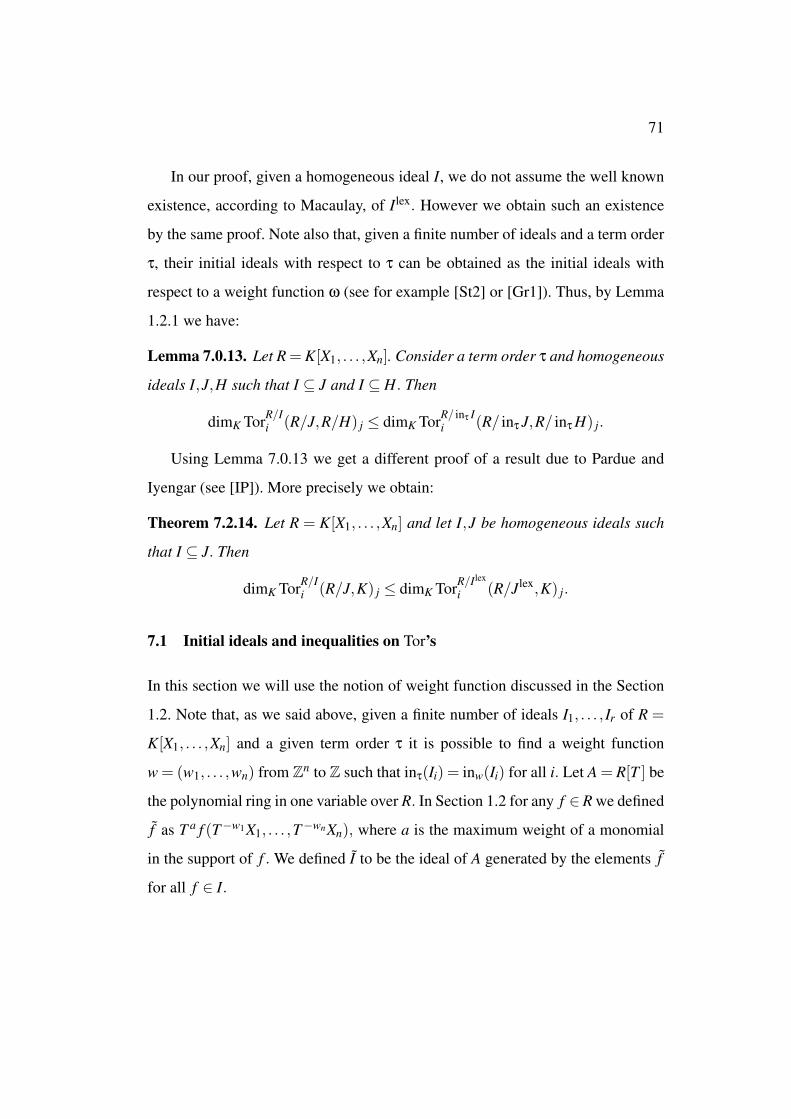
71

In our proof, given a homogeneous ideal I, we do not assume the well known

existence, according to Macaulay, of Ilex. However we obtain such an existence

by the same proof. Note also that, given a finite number of ideals and a term order

τ, their initial ideals with respect to τ can be obtained as the initial ideals with

respect to a weight function ω (see for example [St2] or [Gr1]). Thus, by Lemma

1.2.1 we have:

Lemma 7.0.13. Let R = K[X1, . . . ,Xn]. Consider a term order τ and homogeneous

ideals I,J,H such that I ⊆ J and I ⊆ H. Then

dimK TorR/Ii (R/J,R/H) j ≤ dimK TorR/ inτ I

i (R/ inτ J,R/ inτ H) j.

Using Lemma 7.0.13 we get a different proof of a result due to Pardue and

Iyengar (see [IP]). More precisely we obtain:

Theorem 7.2.14. Let R = K[X1, . . . ,Xn] and let I,J be homogeneous ideals such

that I ⊆ J. Then

dimK TorR/Ii (R/J,K) j ≤ dimK TorR/Ilex

i (R/Jlex,K) j.

7.1 Initial ideals and inequalities on Tor’s

In this section we will use the notion of weight function discussed in the Section

1.2. Note that, as we said above, given a finite number of ideals I1, . . . , Ir of R =

K[X1, . . . ,Xn] and a given term order τ it is possible to find a weight function

w = (w1, . . . ,wn) from Zn to Z such that inτ(Ii) = inw(Ii) for all i. Let A = R[T ] be

the polynomial ring in one variable over R. In Section 1.2 for any f ∈R we defined

f as T a f (T−w1X1, . . . ,T−wnXn), where a is the maximum weight of a monomial

in the support of f . We defined I to be the ideal of A generated by the elements f

for all f ∈ I.

72

Remark 7.1.1. From the definition it follows that A/((T ) + I) ∼= R/ inτ(I) and

A/((T − 1)+ I) ∼= S/I. Moreover, the above isomorphisms are obtained just by

specializing T at 0 and at 1 respectively. In general, for any c ∈ K with c 6= 0 the

ideal I restricted at T−c= 0 is just D(I)⊂R, where D is the change of coordinates

on R induced by the diagonal matrix with diagonal (c−w1, . . . ,c−wn).

Proposition 7.1.2. Let I be a homogenous ideal of R = K[X1, . . . ,Xn]. Assume that

|K|= ∞, and let I be a set of ideals of R such that for any H ∈ I and any diagonal

matrix D ∈ Gln(K) we have D(H) ∈ I. Given two integers i and j, let J ∈ I be an

ideal such that

dimK Tori(R/I,R/J) j = minH∈I

dimK Tori(R/I,R/H) j.

Then for any term order τ we have

dimK Tori(R/I,R/J) j ≤ dimK Tori(R/ inτ(I),R/J) j.

Proof. Consider a weight function w = (w1, . . . ,wn) such that inw(I) = inτ(I).

Let IT=a with a ∈ K be the ideal of R obtained from I by setting T = a. As

we mentioned above, if a = 0 then IT=0 = inτ(I) otherwise for a 6= 0 we have

IT=a = Da(I) where Da is the diagonal matrix with diagonal (a−w1, . . . ,a−wn). We

can calculate dimK Tori(R/IT=a,R/J) j by taking a resolution of R/J and then ten-

soring with R/IT=a. It is easy to see that we can find two matrices, say Aa and Ba,

whose coefficients are rational functions of a such that dimK Tori(R/IT=a,R/J) j =

dimK(kerAa)−dimK(imBa). Therefore, there exists a non-empty Zariski open set

U ⊂A1K such that for any a∈U the value dimK(kerAa)−dimK(imBa) is constant

and minimum. We have, for any a ∈U and a 6= 0, that:

dimK Tori(R/ inτ(I),R/J) j = dimK Tori(R/IT=0,R/J) j≥ dimK Tori(R/IT=a,R/J) j.

73

Since IT=a = Da(I), we can use the change of coordinates induced by D−1a and

obtain:

dimK Tori(R/IT=a,R/J) j = dimK Tori(R/I,R/D−1a (J)) j ≥ dimK Tori(R/I,R/J) j,

where the last inequality depends on the fact that D−1a (J) ∈ I and on the choice of

the ideal J.

An immediate consequence of Proposition 7.1.2 is the next result, which pro-

vides an extension of formula 7.0.1.

Corollary 7.1.3. Let I be a homogeneous ideal of R = K[X1, . . . ,Xn]. Assume that

|K| = ∞ and let J be an ideal generated by r generic forms of degree d1, . . . ,dr.

Then for any i, j and any term order τ we have:

dimK Tori(R/I,R/J) j ≤ dimK Tori(R/ inτ(I),R/J) j.

Proof. We apply Proposition 7.1.2 by using as I the set of all the homogeneous

ideals of R generated by r forms of degree d1, . . . ,dr.We just have to note that

since the forms generating J are generic we have:

dimK Tori(R/I,R/J) j = minH∈I

dimK Tori(R/I,R/H) j

for all i and j.

An important remark to mention is that Corollary 7.1.3 is just a possible way

to apply Proposition 7.1.2. For example, a similar result to Corollary 7.1.3 can be

obtained by considering any ideal constructed, in a given way, by using sums and

products of generic forms of fixed degrees. For instance let I1 = ( f1, . . . , fa) and

I2 = (g1, . . . ,gb) be two ideals generated by generic forms of degrees d1, . . . ,da

74

and h1, . . . ,hb respectively. Then, setting J = I1I2, the formula of Corollary 7.1.3

still holds. In fact, we can employ Proposition 7.1.2 by using as I the set of all the

homogeneous ideals of R obtained as product of two ideals: one generated by a

forms of degrees d1, . . . ,da and one generated by b forms of degree g1, . . . ,gb.

7.2 Pardue’s method and Macaulay estimate on the Hilbert function ofstandard graded algebras

The aim of this section is to show how to use Pardue’s idea [Pa1] to derive at

once his result and the well-known Macaulay estimate on the Hilbert function of

standard graded algebra. Before going into the details of this proof, we give a

brief introduction to polarizations (which sometimes are called distractions) and

generic specializations. See [Pa1], [BH] Lemma 4.2.16, and [BCR] for further

details.

7.2.1 Polarizations and specializations of monomial ideals

In the literature, polarizations are often used to obtain from a monomial ideal, a

new one which is square-free. For example, given I = (X31 ,X

21 X2

2 )⊂ R = K[X1,X2]

by polarizing we get the ideal J = (T1T2T3,T1T2T4T5) ⊆ S = K[X1,X2,T1, . . . ,T5].

This ideal is square-free and encodes all the information of I, in the sense that

there exists a regular sequence for S/J , precisely: T1−X1,T1−X2,T3−X3,T4−

X2,T5−X2, such that I = (J+(T1−X1,T1−X2,T3−X3,T4−X2,T5−X2))∩R. In

other words, by substituting back X1 for T1 and so on, we obtain the ideal I.

This is the kind of polarization considered by Pardue. For our purposes we

prefer to use certain partial polarizations that do not modify the original ideal too

much.

75

For instance, let I ⊆ R = K[X1, . . . ,Xn]. Choose a distinguished variable, say

Xa, and fix an exponent, say b. Let S be the polynomial ring obtained from R by

adjoining the new variable T(a,b). Let m1, . . . ,ms be the minimal system of mono-

mial generators of J. If mi is divisible by Xba define ni = (mi/Xa)T(a,b), otherwise

set ni = mi. The polarization of I obtained by the choice of (a,b) is the ideal J =

(n1, . . . ,ns)⊂ S. From J it is possible to re-obtain I as I = (J +(T(a,b)−Xa))∩R.

Moreover T(a,b)−Xa is a regular element for S/J.

For example, the polarization of I = (X31 ,X

21 X2

2 )⊂ R = K[X1,X2], with respect

to the variable X1 and the exponent 3 (i.e. the pair (1,3)), is

(X21 T(1,3),X

21 X2

2 )⊂ S = K[X1,X2,T(1,3)].

We want to describe these polarizations in a slightly greater generality.

Definition 7.2.1. Let I ⊂ R = K[X1, . . . ,Xn] be a monomial ideal and let G(I) be

the set of its minimal monomial generators. Define Q to be the following set of

integers pairs: (i, j)|0≤ i≤ n,0 < j and let P⊂Q be a finite subset. Let R[P] be

the polynomial ring over R defined as R[T(i, j)|(i, j) ∈ P]. Given a monomial m ∈ R

we set the monomial P(m) ∈ R[P] to be:

m ·

∏(i, j)∈P and

X ji |m

T(i, j)Xi

.

The polarization of I with respect to P is defined as

P(I) = (P(m)|m ∈ I).

It is easy to verify that P(I) is also equal to (P(m)|m ∈ G(I)).

76

We recall some facts about polarizations that are quite easy to prove.

Remark 7.2.2. Let P ⊂ (i, j)|0 ≤ i ≤ n,0 < j be a polarization and let I and J

be monomial ideals.

(1) Note that, by definition, if I ⊂ J then P(I)⊂ P(J).

(2) Each polarization can be factored as a composition of simpler ones. In fact it

is easy to find a sequence of polarizations P1, . . . ,Ps each of them consisting

of only one pair, such that P(I) = Ps Ps−1 · · · P1(I).

(3) In general, P(I + J) = P(I)+P(J) and P(I∩ J) = P(I)∩P(J).

(4) The elements T(i, j)−Xi, for all (i, j) ∈ P, form a regular sequence for the

ring R[P]/P(I). For a proof of this fact one can read, for example, the proof

of Lemma 4.2.16. in [BH]. Another possible way to see this fact is the fol-

lowing: write I = ∩Ii where the Ii are irreducible monomial ideals, i.e. gen-

erated by pure powers of the variables. By part (2) we can assume that the

polarization consists of only one pair, say (a,b). By part (3) we know that

P(I) = ∩P(Ii). Each one the P(Ii) has at most two associated primes, and

clearly T(a,b)−Xa does not belongs to any of these. Therefore, T(a,b)−Xa is

not contained in any prime associated to P(I).

Remark 7.2.3. For any of the elements T(i, j)− Xi choose a variable, say Xl(i, j) .

Since K is an infinite field, the elements T(i, j)−Xi− λ(i, j)Xl(i, j) , where the λ(i, j)

are generic elements in K, are also a regular sequence for R[P]/P(I). Here generic

means that there exists a non-empty Zariski open set of U ⊂ArK such that the λ(i, j)

can be taken to be the entries of any point in U. This open set is, for example, the

one at which the Hilbert function of P(I)+(T(i, j)−Xi−λ(i, j)Xl(i, j)) is maximal and

77

constant. We will denote the ideal (T(i, j)−Xi−λ(i, j)Xl(i, j)) by W, and by P(I)W the

ideal (P(I)+(W ))∩R, obtained by polarizing and then by specializing using W .

Remark 7.2.4. The idea of Pardue is partially based on the isomorphisms below.

Let P be a polarization and let S = R[P]. Set m and n to be the homogeneous

maximal ideals of R and S respectively. Let V be the ideal of S generated by the

T(i, j)−Xi’s , and let W be the ideal of S generated by the T(i, j)−Xi−λ(i, j)Xl(i, j)’s .

We have:

TorR/Ii (R/J,R/m)∼= TorS/(P(I)+(V ))

i (S/(P(J)+(V )),S/(m+(V )).

Since (m+(V )) = n and V is generated by a regular sequence for both S/P(I)

and S/P(J), we get:

TorS/(P(I)+(V ))i (S/(P(J)+(V )),S/(m+(V ))∼= TorS/P(I)

i (S/P(J),S/(n)).

Now, because we also have that n = (m+(W )), in the same way, we deduce that

TorS/P(I)i (S/P(J),S/(n))∼= TorS/(P(I)+(W ))

i (S/(P(J)+(W )),S/(m+(W )). By de-

noting P(I)W and P(J)W the ideals (P(I)+ (W ))∩R and (P(J)+ (W ))∩R we

obtain:

TorR/Ii (R/J,K)∼= TorR/P(I)W

i (R/P(J)W ,K).

Taking the initial ideal with respect to the lexicographic term order: lex, and

applying Lemma 7.0.13, we deduce:

dimK TorR/Ii (R/J,K) j ≤ dimK TorR/ inlex(P(I)W )

i (R/ inlex(P(J)W ),K) j. (7.2.1)

Remark 7.2.5. An important point to make is that a polarization followed by a

specialization is, in a certain way, similar to performing a change of coordinates

(actually any change of coordinate can be obtained in this way), with the advan-

tages that the characteristic of the base field does not create too many problems.

78

For example, let I = (X21 ,X

22 ) ⊂ K[X1,X2] with char(K) = 2. This ideal is fixed

under any change of coordinates. On the other hand, the polarization P = (2,1)

followed by the specialization W = (T(2,1)−X2−λ(2,1)X1) gives the ideal P(I)W =

(X21 ,X2(X2 +λ(2,1)X1)) and in particular inlex(P(I)W ) = (X2

1 ,X1X2,X32 ).

7.2.2 A total order on the monomial ideals

We now want to consider a total order on the monomial ideals of R induced by a

given term order τ. It will be useful to compare, using τ, monomials of different

degree. For this purpose set m > n whenever deg(m)< deg(n).

Definition 7.2.6. Let I and J be two monomial ideals. Let m1 > m2 > · · · > mr

and n1 > n2 > · · ·> ns be the minimal monomial generators, ordered with respect

to τ, of I and J respectively. We say that I >τ J if I ( J or m1 = n1, . . . ,mi = ni

and mi+1 > ni+1.

Lemma 7.2.7. An increasing sequence of monomial ideals, with respect to the

total order above, eventually stabilizes.

Proof. Given a monomial ideal I we denote by I|i the ideal generated by the i

greatest minimal monomial generators of I. When the number of minimal gener-

ators of I is less than i we define I|i = I.

Let I1 ≤ I2 ≤ . . . be a sequence of monomial ideals. For a given monomial

m there are only a finite number of monomials greater than m and therefore

(I1)|1 ≤ (I2)|1 ≤ (I3)|1 ≤ . . . eventually stabilizes. By induction we can assume

that (I1)|a ≤ (I2)|a ≤ (I3)|a ≤ . . . stabilizes, say at (Ib)|a. As above, we observe

that there are only a finite number of monomials greater than the (a+1)th gener-

ator of Ib and, therefore (I1)|a+1 ≤ (I2)|a+1 ≤ (I3)|a+1 ≤ . . . also becomes stable.

79

We have constructed the chain J1 ⊆ J2 ⊆ J3 ⊆ . . . of the ideals Ji at which the

restriction to the first i generators becomes stable. Since R is Noetherian the chain

of the Ji’s also becomes stable and so does the one of the Ii’s .

Before proving the next lemma it is useful to discuss a different way to com-

pare two monomial ideals by using >τ .

Remark 7.2.8. Let I and J be two monomial ideals such that none of them contains

another. Order decreasingly all the monomials in I, and respectively in J, by τ. In

this way we obtain two sequences of monomial mi∈N and ni∈N. Then I >τ J

if and only if m1 = n1, . . . ,m j = n j and m j+1 > n j+1 for some j.

Consider now the task of comparing the initial ideals of two given homoge-

neous ideals I and J of R = K[X1, . . . ,Xn]. First of all, note that a possible way to

describe all the monomials of in(I) of degree d is the following. Let f1, . . . , fr be

a system of generators for the polynomials in I of degree d. Let t1 > t2 > · · ·> ts

be all the monomials of degree d of R. Write any fi as ∑si ai, jt j, and let A be the

matrix given by the ai, j. Define r(d, j) to be the rank of the submatrix consisting of

the first j columns of A. Then t j ∈ (inτ I)d if and only if r(d, j−1) < r(d, j). Given

a homogeneous ideal I we can construct the sequence pii∈N of non-negative

integers consisting of all the ranks:

r(1,1), . . . ,r(1,dimR1),r(2,1), . . . ,r(2,dimR1) . . . ,r(d,1), . . . ,r(d,dimRd) . . .

Similarly, given another homogenous ideal J we can construct its sequence of the

ranks: qii∈N. Assuming there is no containment between inτ(I) and inτ(J) we

have inτ(I)>τ inτ(J) if and only if p1 = q1, . . . , p j = q j and p j+1 > q j+1 for some

index j.

80

Lemma 7.2.9. Let I be a monomial ideal and τ be a term order. For any polar-

ization P and any generic specialization W = ((T(i, j)−Xi−λ(i, j)Xl(i, j))|(i, j) ∈ P)

we have:

I ≤τ inτ(P(I)W ).

Proof. First of all note that inτ(P(I)W ) is constant for a generic choice of the co-

efficients λ(i, j). To simplify the notation let J = inτ(P(I)W ). Since I and J have

the same Hilbert function it is impossible that one ideal is strictly contained in

another. Using the notation of the above Remark 7.2.8, let pii∈N and qii∈N

be the sequences of ranks of I and J respectively. If, by contradiction, I >τ J then

p1 = q1, . . . , p j = q j and p j+1 > q j+1 for some index j. If all the λ(i, j) were zero

we would have p j+1 = q j+1. On the other hand, choosing generic λ(i, j), the ranks

q j+1 can only increase and therefore p j+1 ≤ q j+1. This contradicts our assump-

tion.

7.2.3 Results of Macaulay and Pardue

We are finally ready to prove the Theorems of Macaulay and Pardue.

Definition 7.2.10. We say that a monomial ideal I is a lex-segment ideal if, in

any degree d, the vector space Id is spanned by a lex-segment, i.e. the greatest

dimK(Id) monomials of degree d with respect to the lexicographic term order.

The next lemma is the keystone of the whole chapter.

Lemma 7.2.11. Let I ⊆ R = K[X1, . . . ,Xn] be a monomial ideal, which is not a

lex-segment ideal. Then there exists a polarization P and a generic specialization

W such that in(P(I)W )>lex I.

81

Proof. By Lemma 7.2.9 it is enough to show that there exists a polarization P and

a generic specialization W such that in(P(I)W ) 6= I. We consider two cases.

First, assume that I is not strongly stable. Then there exists a monomial m and

variables Xi and X j with j < i such that Xi|m but (m/Xi)X j 6∈ I. Set P = (i,1)

and let the generic specialization be W = (T(i,1)−Xi−λ(i,1)X j). The ideal P(I)W

contains (m/Xi)(Xi +λ(i,1)X j) and, therefore, (m/Xi)X j ∈ inlex(P(I)W ).

Second, assume that I is strongly stable but not a lex-segment ideal. Let m1 >

m2 > · · · > mr be the minimal monomial generators of I ordered reverse lexico-

graphically. Since I is not a lex-segment ideal there exists a monomial ms such

that (m1,m2, . . . ,ms−1) is a lex-segment ideal while J = (m1,m2, . . . ,ms) is not.

By Remark 7.2.2 part (1), without loss of generality, we can assume that I = J.

Let Xi be the lowest variable dividing ms and write ms = mXai−1Xb

i , with m be-

longing to K[X1, . . . ,Xi−2]. The lowest monomial greater than ms is mXa+1i−1 Xb−1

n ,

which is not in I since I is not a lex-segment ideal. Let V be the vector space

spanned by all the monomials u of S = K[Xi−1,Xi,Xn] of degree a+ b such that

um ∈ I. Note that (V ) is strongly stable but it is not a lex-segment ideal of S. It

is enough to show that there exists a polarization P and a generic specialization

W for the ring S such that inlex(P((V ))W ) 6= (V ). Similarly, without loss of gener-

ality, we can assume that a = 0. We know that Xbi ∈ V and that Xi−1Xb−1

n 6∈ V.

Let c be the greatest integer less than b such that Xi−1Xci Xb−1−c

n 6∈ V, and let

U be the vector space spanned by all the monomials u of S = K[Xi−1,Xi,Xn] of

degree b− c such that Xci u ∈ V. By substituting V for U , without loss of gener-

ality, we can assume that c = 0. After these reductions, we know that Xbi ∈ V

while Xi−1Xb−1n 6∈ V and all the monomials of degree b which are greater than

Xi−1Xb−1n belong to V. Set P = (i, j)|1 ≤ j ≤ b and let the generic specializa-

82

tion to be W = (T(i,1)−Xi−λ(i,1)Xi−1)+(T(i, j)−Xi−λ(i, j)Xn|1 < j ≤ b). We see

that Xi−1Xb−1n ∈ inlex(P((V ))W ). Thus inlex(P((V ))W ) 6= (V ).

Theorem 7.2.12. (Macaulay) Let I ⊆ R = K[X1, . . . ,Xn] be a homogeneous ideal.

Then there exists a lex-segment ideal J with the same Hilbert function of I.

Proof. By taking the initial ideal with respect to the lexicographic term order,

without loss of generality, we can assume that I is monomial. Using Lemma 7.2.7,

we know that there exists a monomial ideal, say J, maximal with respect to <lex

among the monomial ideals with the same Hilbert function of I. By Lemma 7.2.11

J has to be a lex-segment ideal.

We can now give the definition below.

Definition 7.2.13. Let I ⊆ R = K[X1, . . . ,Xn] be a homogeneous ideal. We denote

by Ilex the only lex-segment ideal with the same Hilbert function of I.

Theorem 7.2.14. (Pardue-Iyengar) Let R = K[X1, . . . ,Xn] and let I,J be homoge-

neous ideals such that I ⊆ J. Then

dimK TorR/Ii (R/J,K) j ≤ dimK TorR/Ilex

i (R/Jlex,K) j.

Proof. By Lemma 7.0.13 we can assume that both I and J are monomial ideals.

Let X be the set of all the pairs of ideals (H,L) such that H ⊆ L, H and L have the

same Hilbert function of I and J respectively, and they satisfy:

dimK TorR/Ii (R/J,K) j ≤ dimK TorR/H

i (R/L,K) j.

By Lemma 7.2.7, let (H,L) be a maximal pair in X with respect to the partial order

induced by <lex. If H or L is not a lex-segment ideal, we can use Lemma 7.2.11

and formula (7.2.1) to contradict the maximality of (H,L).

Chapter 8

Variations on a Theorem of Eakin and Sathaye and on Green’s HyperplaneRestriction Theorem

This chapter has been developed around our observation, presented in [Ca3], that

the following theorem according to Eakin and Sathaye, can be viewed, after some

standard reductions, as a corollary of Green’s Hyperplane Restriction Theorem,

which gives an estimate of the Hilbert function of a generic hyperplane restriction

of a standard graded algebra.

Theorem (Eakin-Sathaye). Let (R,m) be a quasi-local ring with infinite residue

field. Let I be an ideal of R, and let i and p be positive integers. If the number of

minimal generators of Ii, denoted by v(Ii), satisfies

v(Ii)<

(i+ p

p

),

then there are elements h1, . . . ,hp in I such that Ii = (h1, . . . ,hp)Ii−1.

A recent generalization of the above result according to L.O’Carroll [O] gave

us the motivation for the following study (see also [HT] for an interesting proof

of the Eakin-Sathaye Theorem). The idea is that, since it is possible to extend

the Theorem of Eakin and Sathaye, it should be also possible to modify Green’s

Hyperplane Restriction Theorem to recover, as corollaries, the result of O’Carroll.

In fact, this is the case.

84

One interesting part of this approach is that we can actually obtain some fur-

ther generalizations of the work of O’Carroll and at the same time give a general

method for deriving variations of the Theorem of Eakin and Sathaye.

The modification of the Hyperplane Restriction Theorem that we present fol-

lows very closely Green’s original proof [Gr2], with the only difference that we

underline the key-properties he needs to build up the inductive step of his proof.

The chapter is divided as follows. First, we give a short introduction to Ma-

caulay representation of integer numbers. This is needed for the understanding of

the Hyperplane Restriction Theorem.

Second, we prove a more general version of the Hyperplane Restriction The-

orem, putting some emphasis on certain special cases where it can be applied. In

fact, our main goal is to obtain a restriction theorem that does not have to deal nec-

essarily with a generic hyperplane, as it is in Green’s original statement. Roughly

speaking, if we know some extra informations about the algebra, it is possible to

obtain the same estimate on the Hilbert function as Green did by restricting to

some partially generic hyperplane.

Finally, we apply the previous work to obtain variations on the Eakin-Sathaye

Theorem.

8.1 Macaulay representation of integer numbers

The following are, nowadays, quite standard facts. An interested reader may look

at [Sta],[Gr1] or [Gr2] for more details on the subject.

Let d be a positive integer. Any positive integer c can then be uniquely ex-

pressed as

c =(

kd

d

)+

(kd−1

d−1

)+ · · ·+

(k1

1

),

85

where the ki’s are non-negative and strictly increasing, i.e. kd > kd−1 > · · ·> k1 ≥

0. This way of writing c is called the d’th Macaulay representation of c, and the

ki’s are called the d’th Macaulay coefficients of c. For instance, setting c = 13 and

d = 3 we get 13 =(5

3

)+(3

2

)+(0

1

).

Remark 8.1.1. An important property of Macaulay representation is that the usual

order on the integers corresponds to the lexicographical order on the arrays of

Macaulay coefficients. In other words, given two positive integers c1 =(kd

d

)+(kd−1

d−1

)+ · · ·+

(k11

)and c2 =

(hdd

)+(hd−1

d−1

)+ · · ·+

(h11

)we have c1 < c2 if and only

if (kd,kd−1, . . . ,k1) is smaller lexicographically than (hd,hd−1, . . . ,h1).

Definition 8.1.2. Let c and d be positive integers. We define c<d> to be

c<d> =

(kd−1

d

)+

(kd−1−1

d−1

)+ · · ·+

(k1−1

1

)where kd, . . . ,k1 are d’th Macaulay coefficients of c. We use the convention that(a

b

)= 0 whenever a < b.

Remark 8.1.3. It is easy to verify that if c1 ≤ c2 then c1<d> ≤ c2<d>. This prop-

erty, as we see further, allows us to iteratively apply the Restriction Theorem to

derive Corollary 8.2.7.

Defining δ = minm|km ≥m we have the alternate representations c =(kd

d

)+(kd−1

d−1

)+ · · ·+

(kδ

δ

)and c<d> =

(kd−1d

)+(kd−1−1

d−1

)+ · · ·+

(kδ−1δ

). Note also that if

kδ 6= δ then (c−1)<d> < c<d>.

8.2 Green’s Hyperplane Restriction Theorem

Let R be a standard graded algebra over an infinite field K. We can write R as

K[X1, . . . ,Xn]/I where I is a homogeneous ideal. The result of Mark Green we

86

discuss below gives an upper bound for the dimension of the dth graded compo-

nent of R/(l), where l is a linear form, in terms of dimension of the dth graded

component of R. This bound is satisfied generically, in the sense that it holds for

any linear form in a certain non-empty Zariski open set U ⊆ P(R1). In other words

we say that Green’s estimate is satisfied by a generic linear form. In general when

we say that a property (P) is satisfied by r generic linear forms we mean that

there exists a non-empty Zariski open set of U ⊆ P(R1)r such that any r-tuple in

U consists of r linear forms satisfying (P).

Green’s result is the following:

Theorem 8.2.1 (Green’s Hyperplane Restriction Theorem). Let R be a standard

graded algebra over an infinite field K, and let l be a generic linear form of R.

Setting S to be R/(l), we have

dimk Sd ≤ (dimK Rd)<d>.

The Hyperplane Restriction Theorem first appeared in [Gr2] where it was

proved with no assumption on the characteristic of the base field K.

A more combinatorial proof can be found in [Gr1] where the characteristic

zero assumption is a working hypothesis. A person interested in reading this last

proof can observe that, with a few minor changes, the arguments in [Gr1] also

work in positive characteristic.

It is important to recall that the numerical bound of Theorem 8.2.1 can be also

interpreted in the following way: let A = K[X1, . . . ,Xn] and let I ⊂ A be a homoge-

neous ideal. Define J = Ilex ⊂ A to be the lex-segment ideal with the same Hilbert

function as I. Let c be the dimension, as a K-vector space, of (A/I)d. By defini-

tion we also have that dimK(A/J)d = c. It is possible to show that dimK(A/(J +

87

(Xn))d = c<d>. Then, for any degree d, Theorem 8.2.1 is equivalent to

dimK(A/I +(l))d ≤ dimK(A/Ilex +(Xn))d.

Recently, in this respect, Aldo Conca has proved the following stronger result

that we have discussed in the previous chapter, see formula (7.0.2): assume the

characteristic of K to be zero and let ln, . . . , lr be generic linear forms of A, then

dimK Tori(A/I,A/(ln, . . . , lr)) j ≤ dimK Tori(A/Ilex,A/(Xn, . . . ,Xr)) j. Conca’s re-

sult, when the index of the Tor is equal to zero, gives Theorem 8.2.1 in char-

acteristic zero.

We want to modify Green’s result in a rather different direction. Our main

focus is to substitute the genericity condition for the linear form with some weaker

assumption. Assume, for example, that the standard graded algebra in Green’s

result is a quotient of the following toric algebra:

S = K[XiYj|0≤ i≤ n1,0≤ j ≤ n2]∼= K[T1, . . . ,Tn1n2]/I.

It is reasonable to think that, for such an algebra, the product of a generic linear

forms in the Xi’s and a generic linear forms in the Yj’s may satisfy the bound

of Theorem 8.2.1. This is in fact true, as we will see further, even though such

an element is not generic. The forms of this type belong in fact to a non-trivial

Zariski closed set of the projective space of linear forms.

Before proving our version of the Hyperplane Restriction Theorem we have to

introduce some notation.

Definition 8.2.2. Let R be a standard graded algebra and let l1, . . . , lr be a set

of linear forms. Let I0,0 = (0) and I1,0 = (l1). For 0 < i ≤ r and 0 ≤ j < d

inductively define the set Ii,j to be

Ii,j = (I : li)|I ∈ Ii−1,j−1∪I +(li)|I ∈ Ii−1,j.

88

Note that the first index keeps track of how many linear forms have been used and

the second one indicates the number of colons that have been performed.

We say that l1, . . . , lr are suitable for the Hyperplane Restriction Theorem in

degree d, property (Gr,d), if they satisfy the next three conditions:

(1) For any I ∈ Ii−1,j, with 0 < i≤ r and m 6⊆ I, we have li 6∈ I.

(2) For any I ∈ Ir,j, we have m⊆ I where m is the homogeneous maximal ideal.

(3) For any I ∈ Ii,j, with i≤ r−2 we have:

dimK((I : li+1)+(li+2))d− j−1 ≤ dimK((I + li+1) : li+2)d− j−1.

Remark 8.2.3. Let n = dimK R1. If property (1) holds, then property (2) is auto-

matically satisfied if r ≥ n+ d− 1. Property (3) is implied by the next stronger

condition.

(3’) For any I ∈ Ii,j with 0≤ i≤ r−2, the Hilbert function of ((I : li+1)+ li+2)

agrees with the Hilbert function of ((I : li+2)+ li+1).

In fact if (3’) is satisfied, for any degree a we have

dimK((I : li+1)+(li+2))a = dimK((I : li+2)+(li+1))a ≤ dimK((I +(li+1)) : li+2)a

where the last inequality comes from ((I : li+2)+(li+1))⊆ ((I +(li+1)) : li+2).

Example 8.2.4. At a first sight the properties (Gr,d) may not seem too easy to

verify. However there are several examples for which it is not hard to find linear

forms, not generic, satisfying our condition. We give a list of the most significant

ones for the variations of the Theorem of Eakin-Sathaye we want to prove.

Let R be a standard graded algebra, dimK R1 = n, |K|= ∞. The following are

examples of r linear forms with r ≥ d +n−1, satisfying (Gr,d).

89

(A) With no further assumptions on R the r linear forms can be taken to be

generic.

(B) Assume R to be the homomorphic image of the Segre ring:

S = K[X1,i1 ·X2.i2 · · ·Xs,is|1≤ i1 ≤ n1, . . . ,1≤ is ≤ ns],

under a map sending the monomials X1,i1 ·X2.i2 · · ·Xs,is to linear forms. Then

the r linear forms can be taken to be the images of l1 · · · ls, where li is a

generic linear form of K[Xi,1, . . . ,Xi,ni].

(C) Assume that char(K) = 0 and that R is the homomorphic image of the

Veronese ring: S = K[Xa11 · · ·X

ass |∑s

i=1 ai = b and ai ≥ 0] under a map send-

ing the monomials Xa11 · · ·X

ass to linear forms. Then the r linear forms can be

taken to be the images of lb, where l is a generic linear form of K[X1, . . . ,Xs].

(D) Assume that char(K) = 0 and that R is the homomorphic image of Segre

products of Veronese rings:

S = K

∏1≤i≤s

1≤ j≤ni

Xai, ji, j such that ∑

jai, j = bi and ai, j ≥ 0

under a map sending the monomials ∏Xai, j

i, j to linear forms. Then the r linear

forms can be taken to be the images of lb11 · · · l

bss , where li is a generic linear

form of K[Xi,1, . . . ,Xi,ni].

(E) Assume that char(K) = 0 and that R is the homomorphic image of the fol-

lowing toric ring:

S = K[Xi1 ·Xi2 · · ·Xis|1≤ i1 ≤ n1, . . . ,1≤ is ≤ ns and n1 ≤ n2 ≤ ·· · ≤ ns]

90

under a map sending the monomials Xi1 ·Xi2 · · ·Xis to linear forms. Then the r

linear forms can be taken to be the images of l1(l1+ l2) · · ·(l1+ l2+ · · ·+ ls),

where li is a generic linear form of K[Xni−1, . . . ,Xni].

Proof. It is easy to see that in all the examples above the elements of S we consider

belong to some products of projective spaces. For example, in (B) an element

written as l1 · · · ls, where li is a linear form of K[Xi,1, . . . ,Xi,ni], corresponds, up

to scalars, to a point in V = Pn1−1×Pn2−1× ·· ·×Pns−1. We have to show that

there exists a non-empty open set of W = V r whose r-tuple satisfy (GR,d). First

of all, note that (2) is satisfied since there exists an open set of U ⊆W such that

any n entries of the points of U are generators for the homogeneous maximal

ideal. Here is where we need the characteristic zero assumption for some of the

examples, otherwise our linear forms may not generate the homogeneous maximal

ideal. Thus we can find a non-empty open set where (1) and (2) are satisfied.

Part (3) needs more explanation. Once we fixed an r-tuple, i.e. a point in W,

any ideal in Ii,j can be identified with a precise sequence of operations: sums

and colons. For any sequence there exists a non-empty Zariski open set of W

for which the Hilbert function of the ideal constructed using such a sequence is

constant. Since r is fixed, the number of possible sequences of sums and colons

is finite. Therefore, there exists a non-empty Zariski open set U ⊂W such that

any ideal in any of the Ii,j′s has a Hilbert function constant on U , which depends

only on the sequence of operations defining the ideal. Since U ⊂W =V r is open

and non-empty, we can find an open and non-empty subset of U closed under any

permutation of the r entries of its elements. Thus, property (3’) is satisfied by the

r-tuples of such open set. In particular, by Remark 8.2.3, condition (3) holds.

Remark 8.2.5. Note that the characteristic assumption in (C),(D) and (E) is es-

91

sential. Let R = K[X21 ,X1X2,X2

2 ]/(X21 ,X

22 )∼= K[Y1,Y2,Y3]/(Y1,Y3,Y 2

2 −Y1Y3) and

assume char(K) = 2. This correspond to the case s = 2 and b = 2 of example (C).

The square of a generic linear form of K[X1,X2] can be written as X21 +λX2

2 and

it has a zero image in R. Property (2) of (Gr,d) is not satisfied. Moreover, a zero

linear form clearly does not satisfy Green’s estimate.

We can now prove the Hyperplane Restriction Theorem. The structure of the

proof is exactly the same as in Green’s paper [Gr2].

Theorem 8.2.6. Let R be a standard graded algebra and let l1, . . . , lr be linear

forms satisfying (Gr,d). Then

dimK(R/(l1))d ≤ (dimK(Rd))<d>.

Proof. Since (0) ∈ I0,0, in order to prove the theorem it is enough to show:

Claim. For any I ∈ Ii,j with i < r we have:

dimK(R/(I +(li+1)))d− j ≤ (dimK(R/I)d− j)<d− j>. (8.2.1)

First of all, we show that the claim holds for all the ideals in Ir−1,j and in Ii,d−1.

By part (2) of (Gr,d), since I ∈ Ir−1,j then m⊆ (I+(lr)) ∈ Ir,j. Because j < d we

have (R/(I+(lr)))d− j = 0 and, therefore, the inequality (8.2.1) holds. If I ∈ Ii,d−1

the inequality (8.2.1) becomes dimK(R/(I + (li+1)))1 ≤ dimK(R/I)1− 1 and it

follows from the part (1) of (Gr,d).

We do a decreasing induction on the double index of Ii,j.

Let I ∈ Ia,d−b with a < r− 1 and b > 1. By induction we know that (8.2.1)

holds for (I + (la+1)) ∈ Ia+1,d−b and for (I : la+1) ∈ Ia+1,d−b+1. Consider the

sequence below:

0→ R(I +(la+1)) : la+2

(−1)·la+2−−→ R

I +(la+1)→ R

I +(la+1)+(la+2)→ 0.

92

By looking at the graded component of degree b we get:

dimK

(R

I +(la+1)

)b= dimK

(R

(I +(la+1)) : la+2

)b−1

+

+dimK

(R

I +(la+1)+(la+2)

)b.

Property (3) of (Gr,d) implies

dimK

(R

(I +(la+1)) : la+2

)b−1≤ dimK

(R

(I : la+1)+(la+2)

)b−1

,

and by using the inductive assumption on I : la+1 and on I +(la+1) we know that

dimK

(R

I+(la+1)

)b≤(

dimK

(R

I:la+1

)b−1

)<b−1>

+(

dimK

(R

I+(la+1)

)b

)<b>

.

To simplify the notation, set c = dimK(R/I)b and cH = dimK(R/(I +(l1)))b.

From the short exact sequence

0→ RI : la+1

(−1)la+1−−→ R

I→ R

I +(la+1)→ 0

we know that dimK

(R

I:la+1

)b−1

= c− cH , therefore the above upper bound for

dimK

(R

I+(la+1)

)b

becomes:

cH ≤ (cH)<b>+(c− cH)<b−1>. (8.2.2)

Write cH =(kb

b

)+(kb−1

b−1

)+ · · ·+

(kδ

δ

). The inequality of the claim, i.e. cH ≤ c<b>,

is equivalent to c≥(kb+1

b

)+(kb−1

b−1

)+ · · ·+

(kδ+1δ

).

If the claim fails we have:

c− cH <

(kb

b−1

)+

(kb−1

b−2

)+ · · ·+

(kδ

δ−1

). (8.2.3)

We use (8.2.2) to derive a contradiction. There are two cases to consider.

If δ = 1 then (8.2.3) becomes c− cH ≤( kb

b−1

)+(kb−1

b−2

)+ · · ·+

(k21

).

93

Thus

(c− cH)<b−1> ≤(

kb−1b−1

)+

(kb−1−1

b−2

)+ · · ·+

(k2−1

1

)and

(cH)<b> ≤(

kb−1b

)+

(kb−1−1

b−1

)+ · · ·+

(k2−1

2

)+

(k1−1

1

).

By adding these two inequalities, (8.2.2) gives

cH ≤(

kb

b

)+

(kb−1

b−1

)+ · · ·+

(k1−1

1

)< cH ,

which is a contradiction.

If δ > 1 then the equation (8.2.3) is c− cH <( kb

b−1

)+(kb−1

b−2

)+ · · ·+

( kδ

δ−1

)and

since kδ−1 > δ−1 applying b−1 the strict inequality is preserved and gives

(c− cH)<b−1> <

(kb−1b−1

)+

(kb−1−1

b−2

)+ · · ·+

(kδ−1δ−1

).

Adding the last inequality with (cH)<b> ≤(kb−1

b

)+(kb−1−1

b−1

)+ · · ·+

(kδ−1δ

)we

obtain the following contradiction

cH <

(kb

b

)+

(kb−1

b−1

)+ · · ·+

(k1

1

)= cH .

A direct consequence of Theorem 8.2.6 is the corollary below.

Corollary 8.2.7. Let R be a standard graded algebra and let l1, . . . , lr be lin-

ear forms satisfying (Gr,d), and let the Macaulay representation of dimK(Rd) be(kdd

)+(kd−1

d−1

)+ · · ·+

(k11

). Then for any p such that 1≤ p≤ r we have

dimK(R/(l1, . . . , lp))d ≤(

kd− pd

)+

(kd−1− p

d−1

)+ · · ·+

(k1− p

1

).

Proof. By Theorem 8.2.6 we have dimK(R/(l1))d ≤(kd−1

d

)+(kd−1−1

d−1

)+ · · ·+(k1−1

1

). Note that the images of l2, . . . , lr satisfy (Gr,d) for R/(l1). We can, there-

fore, apply Theorem 8.2.6 and obtain the result by induction.

94

8.3 Variations of the Theorem of Eakin and Sathaye

We now prove a general version of the Theorem of Eakin and Sathaye.

Theorem 8.3.1. Let (A,m) be a quasi-local ring with infinite residue field K. Let

I be an ideal of A. Let i and p be positive integers. If the number of minimal

generators of Ii, denoted by v(Ii), satisfies v(Ii)<(i+p

i

)then

(a) (Eakin-Sathaye) There are h1, . . . ,hp in I such that Ii = (h1, . . . ,hp)Ii−1.

Moreover:

(b) (O’Carroll) If I = I1 · · · Is, where I j’s are ideals of R, then we can find the

elements h j’s of the form l1 · · · ls with li ∈ Ii.

(c) Assume char(K) = 0. If I = Jb , where J is an ideal of A, then we can find

the elements h j’s of the form lb with l ∈ I.

(d) Assume char(K) = 0. If I = Ib11 · · · I

bss , where I j’s are ideals of A, then we can

find the elements h j’s of the form lb11 · · · l

bss with li ∈ Ii.

(e) Assume char(K) = 0. If I = I1(I1+ I2) · · ·(I1+ · · ·+ Is), where I j’s are ideals

of A, then we can find the elements h j’s of the form l1(l1+ l2) · · ·(l1+ · · ·+ ls)

with li ∈ Ii.

Proof. First of all, note that since v(Ii) is finite, without loss of generality we can

assume that I is also finitely generated: in fact, if H ⊆ I is a finitely generated

ideal such that H i = Ii the result for H implies the one for I. Similarly, we can

also assume that the ideals I j of (b),(d) and (e) and the ideal J of (c) are finitely

generated. By the use of Nakayama’s Lemma, we can replace I by the homoge-

neous maximal ideal of the fiber cone R =⊕

i≥0 Ii/mIi. Note that R is a standard

95

graded algebra finitely generated over the infinite field R/m = K. Moreover, the

algebras R of (a),(b),(c),(d),(e) satisfy the properties of the Example 8.2.4 parts

(A),(B),(C),(D), and (E) respectively. Let l1, . . . , lr as in Example 8.2.4 and assume

also that p ≤ r. The theorem is proved if we can show that (R/(l1, . . . , lp))i = 0.

Note that dimK Ri ≤(i+p

i

)− 1 =

(i+p−1i

)+(i+p−2

i−1

)+ · · ·+

(i+p− ji− j+1

)+ · · ·+

(r1

).

This can be proved directly or by using Remark 8.1.1. In fact, one can first order

the array of Macaulay coefficients using the lexicographic order and then note that

the previous array of (i+ p,0, . . . ,0) is given by (i+ p− 1, i+ p− 2, . . . , p). By

Corollary 8.2.7 we deduce

dimK(R/(l1, . . . , lp))i ≤(

i−1i

)+

(i−2i−1

)+ · · ·+

(01

).

The term on the right hand side is zero and therefore the theorem is proved.

The general principle behind this proof is that in passing to the fiber cone of

R the properties of the ideal I allow us to conclude that R is the quotient of some

particularly nice toric ring. In such a ring it is quite easy to find interesting l1, . . . , lr

satisfying (Gr,d). Finally, a pre image of l1, . . . , lr gives an interesting reduction for

the ideal I.

References

[An] D. Anick. On the homology of associative algebras. Trans. Amer. Math.

Soc. 296 (1986), no. 2, 641–659.

[AH] A. Aramova, J. Herzog. Koszul Cycles and Eliahou-Kervaire Type Reso-

lutions. J. Algebra 181 (1996), 347-370.

[BM] D. Bayer, D. Mumford. What can be computed in Algebraic Geome-

try? Computational algebraic geometry and commutative algebra (Cor-

tona 1991), 1–48, Sympos. Math., XXXIV, Cambridge Univ. Press, Cam-

bridge, 1993.

[BS] D. Bayer, M. Stillman. A criterion for detecting m-regularity. Invent.

Math. 87 (1987) 1-11.

[BCR] A. Bigatti, A. Conca, L. Robbiano. Generic initial ideals and distractions.

Preprint

[Bl] S. Blum. Subalgebras of bigraded Koszul algebras. J. Algebra 242 (2001),

no. 2, 795–809.

97

[BGT] W. Bruns, J. Gubeladze, Ngo Viet Trung. Normal polytopes, triangula-

tions, and Koszul algebras. J. Reine Angew. Math. 485 (1997), 123–160.

[BH] W. Bruns, J. Herzog. Cohen-Macaulay rings, Cambridge Studies in Math-

ematics 39, Cambridge University Press, Cambridge, 1993.

[BHV] W. Bruns, J. Herzog, U. Vetter. Syzygies and walks. ICTP Proceedings

’Commutative Algebra’, A.Simis, N.V.Trung, G.Valla, eds., World Sci-

entific 1994, 36–57.

[Ca1] G. Caviglia. Bound on the Castelnuovo-Mumford regularity of tensor

product, Proc. AMS, to appear.

[Ca2] G. Caviglia. The pinched Veronese is Koszul, J.Alg.Comb., to appear.

[Ca3] G. Caviglia. A Theorem of Eakin and Sathaye and Green’s Hyperplane

Restriction Theorem Proceedings of the Lisbon Conference on Commu-

tative Algebra 2003, to appear.

[CS] G. Caviglia, E. Sbarra. Characteristic-free bound for the Castelnuovo-

Mumford regularity, Comp.Math., to appear.

[Ch] K. Chandler. Regularity of the powers of an ideal. Comm. Algebra 25

(1997), no.12, 3773–3776.

[Co] A. Conca. Kosul homology and extremal properties of Gin and Lex.

Trans. Amer. Math. Soc. 356 (2004),no. 7, 2945–2961.

[CoCoA] CoCoATeam. CoCoA: a system for doing Computations in Commuta-

tive Algebra. Available at http://cocoa.dima.unige.it

98

[CH] A. Conca, J. Herzog. Castelnuovo-Mumford regularity of products of ide-

als Collect. Math. 54 (2003), no. 2, 137–152.

[CHTV] A. Conca, J. Herzog, Ngo Viet Trung, G. Valla. Diagonal subalgebras

of a bigraded algebras and embeddings of blow ups of projective spaces.

American Journal of Mathematics 119.

[CTV] A. Conca, Ngo Viet Trung, G.Valla. Koszul property for points in projec-

tive spaces, 1998, Mathematica Scandinavica.

[CTRV] A. Conca, Ngo Viet Trung, M. Rossi, G. Valla. Grobner flags and Goren-

stein algebras. Compositio Math. 129 (2001), no. 1, 95–121.

[ES] P. Eakin, A. Sathaye. Prestable ideals. J. Algebra 45 (1976), no. 2, 439–

454.

[Ei] D. Eisenbud. Commutative Algebra with a View Toward Algebraic Ge-

ometry. Springer-Verlag, New York, 1995.

[EG] D. Eisenbud, S. Goto. Linear free resolutions and minimal multiplicity. J.

Algebra 88 (1984), 89–133.

[ERT] D. Eisenbud, A. Reeves and B. Totaro. Initial ideals, Veronese subrings,

and rates of algebras. Adv. Math. 109 (1994), 168–187.

[EK] S. Eliahou, M. Kervaire. Minimal resolutions of some monomial ideals.

J. Algebra 129 (1990), 1–25.

[Fr] R. Froberg. Koszul algebras. Advances in commutative ring theory (Fez,

1997), 337–350, Lecture Notes in Pure and Appl. Math.,205, Dekker,

New York, 1999.

99

[Ga1] A. Galligo. Theoreme de division et stabilite en geometrie analytique lo-

cale. Ann. Inst. Fourier (Grenoble) 29 (1979), 107–184.

[Ga2] A. Galligo. A propos du theorem de preparation de Weierstrass. Springer

Lect. Notes in Mathematics 409 (1973), 543–579.

[GGP] A. Geramita, A. Gimigliano,Y. Pitteloud. Graded Betti numbers of some

embedded rational n-folds. Math. Ann. 301 (1995), no. 2, 363–380.

[Gi] M. Giusti. Some effectivity problems in polynomial ideal theory. Eu-

rosam 84. Springer Lect. Notes in Computer Sciences 174 (1984), 159–

171.

[Go] G. Gotzmann. Eine Bedingung fur die Flachheit und das Hilbertpolynom

eines graduierten Ringes. Math. Z. 158 (1978), 61–70.

[M2] D. Grayson, M. Stillman. Macaulay 2: a software system for alge-

braic geometry and commutative algebra, available over the web at

http://www.math.uiuc.edu/Macaualy2.

[Gr1] M. Green. Generic initial ideals. Six lectures on commutative algebra.

Papers from the Summer School on Commutative Algebra held in Bel-

laterra, July 16–26, 1996. Progress in Mathematics, 166, 119–186.

[Gr2] M. Green. Restrictions of linear series to hyperplanes, and some results

of Macaulay and Gotzmann. Algebraic curves and projective geometry

(Trento, 1988), 76–86, Lecture Notes in Math., 1389, Springer, Berlin,

1989.

100

[HHR] J. Herzog, T. Hibi, G.Restuccia. Strongly Koszul algebras. Math. Scand.

86 (2000), 161–178.

[HP] J. Herzog, D. Popescu. On the regularity of p-Borel ideals. Proc. Amer.

Math. Soc. 129 (2001), no. 9, 2563–2570.

[HT] Le Tuan Hoa, Ngo Viet Trung. Borel-fixed ideals and reduction number.

J. Algebra 270 (2003), no. 1, 335–346.

[IP] S. Iyengar, K. Pardue. Maximal minimal resolutions. J. Reine Angew.

Math. 512 (1999), 27–48.

[Ke] G. Kempf. Syzygies for points in projective space. J. Algebra 145 (1992),

no. 1, 219–223.

[Mal] B. Malgrange. Cartan involutiveness = Mumford regularity. Commutative

Algebra: Interactions with Algebraic Geometry, Contemporary Mathe-

matics, 331.

[Mat] H.Matsumura. Commutative ring theory. Translated from the Japanese by

M. Reid. Second edition. Cambridge Studies in Advanced Mathematics,

8. Cambridge University Press, Cambridge, 1989

[MM] E. Mayr, A. Meyer. The complexity of the word problem for commutative

semigroups and polynomial ideals. Advances in Math. 46 (1982), 305–

329.

[Mu] D.Mumford. Lectures on curves on an algebraic surface. With a section

by G. M. Bergman. Annals of Mathematics Studies, No. 59 Princeton

University Press, Princeton, N.J. 1966 xi+200 pp.

101

[O] L. O’Carroll. Around the Eakin-Sathaye Theorem. Preprint 2004.

[Pa1] K. Pardue. Nonstandard borel-fixed ideals. Thesis, Brandeis University,

1994.

[Pa2] K. Pardue. Deformation classes of graded modules and maximal Betti

numbers. Illinois Journal of Mathematics 40(4) (Winter 1996), 564–585.

[Sa] J. Sally. Numbers of generators of ideals in local rings. Marcel Dekker,

Inc., New York-Basel, 1978.

[Si] J.Sidman. On the Castelnuovo-Mumford regularity of products of ideal

sheaves. Adv. Geom. 2 (2002), no.3, 219–229.

[Sta] R. Stanley. Hilbert Function of graded algebra. Advances in Math 28,

(1978), 57–83.

[St1] B. Sturmfels. Four counterexamples in combinatorial algebraic geometry.

J. Algebra 230 (2000), no. 1, 282–294.

[St2] B. Sturmfels. Grobner bases and convex polytopes. University Lecture

Series, 8. American Mathematical Society, Providence, RI, 1996. xii+162

pp.

[Ta] J. Tate. Homology of Noetherian rings and local rings. Illinois J. Math. 1

(1957), 14–27.