knowledge based image annotation refinementlkhan/papers/knowledge-based image annotation... ·...

Knowledge Based Image Annotation Refinement

Yohan Jin & Latifur Khan & B. Prabhakaran

Received: 26 May 2009 /Revised: 26 May 2009 /Accepted: 26 May 2009 /Published online: 25 September 2009# 2009 The Author(s). This article is published with open access at Springerlink.com

Abstract Recently, images on the Web and personalcomputers are prevalent around the human’s life. Toretrieve effectively these images, there are many (Automat-ic Image Annotation) AIA algorithms. However, it stillsuffers from low-level accuracy since it couldn’t overcomethe semantic-gap between low-level features (‘color’,‘texture’ and ‘shape’) and high-level semantic meanings(e.g., ‘sky’, ‘beach’). Namely, AIA techniques annotatesimages with many noisy keywords. In this paper, wepropose a novel approach that augments the classical modelwith generic knowledge-based, WordNet. Our novel ap-proach strives to prune irrelevant keywords by the usage ofWordNet. To identify irrelevant keywords, we investigatevarious semantic similarity measures between keywordsand finally fuse outcomes of all these measures together tomake a final decision using Dempster-Shafer evidencecombination. Furthermore, We can re-formulate the remov-al of erroneous keywords from image annotation probleminto graph-partitioning problem, which is weighted MAX-CUT problem. It is possible that we have too manycandidate keywords for web-images. Hence, we need tohave deterministic polynomial time algorithm for MAX-CUT problem. We show that finding optimal solution forremoving noisy keywords in the graph is NP-Completeproblem and propose a new methodology for Knowledge

Based Image Annotation Refinement (KBIAR) using adeterministic polynomial time algorithm, namely, random-ized approximation graph algorithm. Finally, we demon-strate the superiority of this algorithm over traditional oneincluding the most recent work for a benchmark dataset.

Keywords Image annotation . Image annotationrefinement .WordNet . Semantic-similarity . Max-cutalgorithm

1 Introduction

At present, sales of digital cameras have, since the first halfof 2003, been surpassed by camera phones. It has beenforecast that 860 million camera phones will be shipped in2009, accounting for 89% of all mobile phone handsets(InfoTrends/Cap Ventures). Where multimedia research isconcerned, camera phones pose a new challenge bygenerating a huge amount of images that arise in connec-tion with the management of thousands of personal photocollections. Given such large image databases, we need tocome up an efficient image retrieval system. For efficientcontent recognition and retrieval, we need metadata of images(description of images). Current search engines like Google,Yahoo, including mobiles (e.g., Google Mobile, and Yahoo!Mobile) rely on keyword based retrieval. In many scenarios,we want to find the images related to a specific concept (forexample, tiger) or we want to find the keywords that bestdescribe the contents of an unseen image [13]. Hence, theefficient solution in these scenarios raises the possibility ofseveral interesting applications such as automated imageannotation, browsing support, and auto-illustrate.

Content-based image retrieval (CBIR) computes rele-vance based on the visual similarity of low-level image

J Sign Process Syst (2010) 58:387–406DOI 10.1007/s11265-009-0391-y

This work has been completed when Jin was enrolled at University ofTexas, Dallas.

Y. Jin (*)Data Mining Team, MySpace (Fox Interactive Media),Beverly Hills, CA 90210, USAe-mail: [email protected]

L. Khan : B. PrabhakaranDepartment of Computer Science, University of Texas at Dallas,Richardson, TX 75080, USA

features such as color histograms, textures, shapes, andspatial layout. However, the problem is that visualsimilarity is not semantic similarity. There is a gap betweenlow-level visual features and semantic meanings. The so-called semantic gap is the major problem that needs to besolved for most CBIR approaches. For example, a CBIRsystem may answer a query request for ‘red ball’ with animage of a ‘red rose’. If we provide annotation of imageswith keywords, then a typical way to publish an image datarepository is to create a keyword-based query interface toan image database. Images are retrieved if they contain(some combination of the) keywords specified by the user.

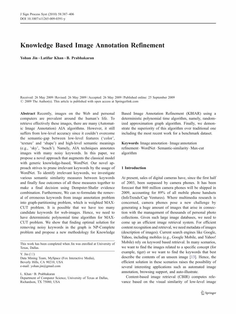
To achieve all these goals several statistical models havebeen proposed. For example, the translation model (TM)[13], the cross-media relevance model (CMRM) [15] and acontinuous relevance model (CRM) [18] can determine aset of keywords that describe visual objects/regions whichappear in an image. However, whatever model we employthe current annotation accuracy is quite low due to theexistence of too many noisy words. Therefore, it is quitedifficult to get a meaningful understanding of images in thismanner. Furthermore, it is impossible to distinguishbetween some keywords such as valley and mountain,garden and tree, cat and tiger, as designations of imagecontent (these keywords are part of the Corel keywords).When a user query is for valley, and the retrieved imagesinclude mountains, the user will be satisfied with this result.Hence, our goal is to facilitate the steps which need to betaken to achieve a semantic understanding of images. Thesemantic meaning of an image will be described by a set ofkeywords, For example, In Fig. 1, two images includepeople, however, the context of people in each image is dif-ferent. The first image (384008) has the keyword-‘the peopleon the beach’ and the second has the keyword-‘the people inthe garden’. Noisy keywords for the first and second imagesIn Fig. 1, are ‘desert snow’ and ‘rock goat’ respectively.

To remove noisy keywords for an image we will utilizethe context of keywords based on semantic similarity. A setof co-occurring keywords that appear in an image willdetermine context. Intuitively, non-correlated keywordsmay be treated as noisy, and discarded. The basic notionof pruning is that a set of keywords associated in an imageoccurring together determine a context for one another,according to which the appropriate senses of the keyword(its appropriate concept) can be determined. Note, forexample, that base, bat, glove may have several interpre-tations as individual terms, but when taken together in animage, the intent is obviously a reference to baseball. Thereference follows from the ability to determine a context forall the keywords. For example, the correlation between‘beach and sand’ that gives a context is greater than ‘snowand sand’ based on semantic similarity given in aknowledge based context, WordNet, and ‘snow’ will bediscarded. On the other hand, ‘people beach’, and ‘peoplegarden’ are both highly correlated.

We will discard an annotated keyword from an imagewhich does not correlate with other annotated keywordsthat appear in the image. For this, first, we investigatevarious semantic similarity measures between keywordswith the usage of WordNet. Each semantic similaritymeasure tries to find the distance between keywords usingseveral different approaches (e.g., node-based, edge-based,gloss-based). In our previous work, we fused thesemeasures Dempster Shafer [1, 36] to make a final decision.In this paper, we also propose a new way of bridging the gapbetween KBIAR problem and the graph approximationproblem. This approach has two important main impacts.First, almost all previous approaches use heuristic thresholdsfor deciding un-related keywords during re-ranking process.Different from heuristic the optimal method, our proposingthe graph approximation algorithm (especially, weighted max-cut in this paper) can deterministically decide noisy nodes

384008:beach people sand desert snow 147066:people flower garden rock goat

Figure 1 An Example of Anno-tations with having noisy andcorrect keywords.

388 J Sign Process Syst (2010) 58:387–406

(keywords) as one set with having at least 0.8785 ratioperformances to the optimal solution [9]. Second, for theproblem of computation complexity, this randomized ap-proximation algorithm can decide irrelevant set in the graphwithin polynomial time. Finally, we compare our approacheswith traditional one including the most recent work anddemonstrate the superiority of our algorithm.

This paper is organized as follows: Section 2 presentsknowledge-based image annotation refinement mechanismsincluding previous work and motivation. Section 3 explainsseveral semantic similarity measures from WordNet alongwith shortcomings, and presents the motivation behindvarious measures. Section 4 presents a modification ofTranslation model along with Demster Shafer evidencetheory. Section 5 presents how we can apply approximatedgraph algorithm in KBIAR problem in polynomial time.

2 Knowledge-Based Image Annotation Refinement

A. Previous work

We can classify most of existing automatic imageannotation algorithms into two categories. First, theyformulate automatic image annotation to classificationproblem with considering keyword (concept) as a uniqueclass of the classifier, which are SVM classifier [32, 34,37], Gaussian Mixture Hierarchical Model [27, 28], BayesPoint Machines [31], 2-dimensional Multi-resolution HiddenMarkov Model [19] and so on.

Second, many statistical models have been published forimage annotation. Mori et al. [23] used a co-occurrencemodel, which estimates the correct probability by countingthe co-occurrence of words with image objects. [13] strivedto map keywords to individual image objects. Both treatedkeywords as one language and blob-tokens as anotherlanguage, allowing the image annotation problem to beviewed as translation between two languages. Using someclassic machine translation models, they annotated a test setof images based on a large number of annotated trainingimages. Based on translation model, Pan et al. [26] haveproposed various methods to discover correlations betweenimage features and keywords. They have applied correla-tion and cosine methods and introduced SVD as well, butthe work is still based on a translation model with theassumption that all features are equally important and noknowledge (KB) base has been used. The problem of thetranslation model is that frequent keywords are associatedwith too many different image segments but infrequentkeywords have little chance of appearing in the annotation.To solve this problem, F. Kang et al. propose two modifiedtranslation models for automatic image annotation andachieve better results [17]. Jeon et al. [15] introduce cross-

media relevance models (CMRM) where the joint distribu-tion of blobs and words is learned from a training set ofannotated images. Unlike translation model, CMRMassumes there is a many to many correlation betweenkeywords and blob tokens rather than one to one.Therefore, CMRM naturally takes into account contextinformation. Furthermore, Lavrenko et al. [18] propose acontinuous relevance model by partitioning an image into afixed number of grids and avoiding segmentation andclustering issues that are observed in previous models.However, in all of this work annotation contains manynoisy keywords and there is no attempt to extends this“limit” of automatic image annotation problem.

B. Motivation

In that, there exists “semantic gap” between concept(keyword) and low-level visual feature values. The way ofimage understanding for human is not depend on low-levelvisual feature, but human would like to rely on their“knowledge” which came from previous personal experi-ences. To bridge the semantic gap, we should try to reflectthe way of human perception for image understanding.WordNet, which is quite famous world knowledge-base forinformation retrieval research area, can be useful resourcefor simulating the human perceptional semantic knowledge.In text retrieval, semantic similarity is very important as abasis for disambiguation and topic classification.

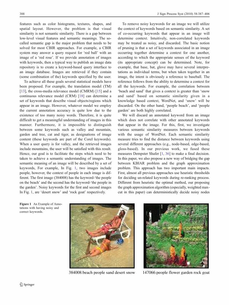
TM model generates a set of keywords, some relevant andsome irrelevant. We consider annotated keywords for animage as words in text document, but there are unrelatedwords. In order to remove irrelevant keywords, we canmeasure semantic similarity between various annotated key-words of images. In Fig. 2, annotated keywords by TM oftwo images (384008, 147066) in Fig. 1, are shown. A set ofkeywords will provide context/semantic of an image. Forexample in Fig. 2, the related keywords in the circle conveysome specified concepts (‘the people in the beach’, ‘thepeople in the garden’) and remove the unrelated keywordsthat appear outside the circle. Here, the circle of semanticsimilarity covers relevant concepts of an image.

C. Image Annotation Improvement through Refinement

Yohan, Khan et al. [1] propose the innovative approachfor improving image annotation using semantic similaritymeasure among annotated keywords. [1] detected irrelevantkeywords among candidate annotated keywords by comb-ing evidence-rule based on semantic similarity in WordNet(TMHD model). For example, if an image has beenannotated with ‘sky’, ‘water’, ‘mountain’, ‘door’ by TMmodel, TMHD model computes the semantic similarity ofone word (yohan et al. [1] called ‘semantic dominance’)over all other candidate words (e.g., ‘sky’ with other

J Sign Process Syst (2010) 58:387–406 389

keywords such as ‘water’, ‘mountain’ and ‘door’). TMHDmodel combined semantic dominance score from threedifferent semantic similarity measurements (JNC, LIN,BNP -see Section 3) and keep only strong candidateannotation keywords whose scores are above the threshold.

Inspired by the idea of Yohan, Khan et al. [1], there havebeen several approaches for improving (automatic imageannotation) AIA problem using the correlation betweenannotated keywords, so called Knowledge-Based ImageAnnotation Refinement(KBIAR) [2–6, 33]. Liu et al. [5]proposes adaptive graphical model for fusing visual contentfeature and keyword correlation. For visual content fea-tures, Liu et al. develop Nearest Spanning Chain. For thecorrelation of keywords, it considers correlation by Word-Net as well as correlation by co-occurrence. Wang et al. [3]propose image annotation refinement by re-ranking theannotations using Random Walk with Restarts algorithm.For random walk restarts, it reformulates image annotationrefinements as a graph ranking problem. For the graphvertices represent each candidate annotation keyword forimages, and “co-occurrence” similarity has been used forthe weight of an edge. Furthermore, Wang et al. [4]proposed a new way of content based image annotationrefinement method as they re-formulating image annotationrefinement problem as a Markov process and candidatekeywords will be assigned to the states of a markov chain.Instead of usingWordNet for semantic similarity, Wang et al.[2] use the Normalized Google Distances (NGD), which isthe distance between two [24] words in terms of contextualrelations. For image annotation refinement process, theypropose conditional random field (CRF) model, which is anundirected graphical model in which a vertex representsconfidence value of each candidate keyword and an edge iscontextual relations between two candidate keywords. Zhou

et al. [6] show an approximation approach for findingoptimal subset annotation keywords of an image based ongreedy algorithm. They use CMRM [15] model formatching probability between image region and keywords.Among several regions of an image, Zhou et al. [6] detectkey-regions by using bipartite graph matching algorithm.

3 Measuring Semantic Similarity

To measure semantic-similarity between two keywords, weuse WordNet and Association rule and will explain these[25] one by one.

A. Semantic Similarity from WordNet

Using semantic similarity, we would like to removenoisy keywords for an image from annotated keywordsgenerated by translation model. However, at the same time,we would like to keep relevant keywords. To do this, firstwe will find relevant concepts from annotated keywords inan image. Next, we will measure similarity between theseconcepts. Finally, some concepts corresponding keywordswill be discarded in which total similarity measure of aconcept with other concepts falls below a certain threshold.

We will use the structure and content of WordNet formeasuring semantic similarity between two concepts. Thecurrent state of the art classifies semantic similarity to threedifferent categories—Node-Based Approach ([16, 22, 29]),Distance-Based Approach ([20]), and Gloss-Based Ap-proach ([12]). In this section, first, we will present variousmeasures to determine semantic similarity between twoconcepts. Second, we will present the drawbacks of eachmeasure. Finally, we will present a hybrid model by fusingthese various measures.

snow

0.62870.5954

0.19840.2343

0.6812

0.3215

flower

garden

rock

goat

people

0.65320.5364

0.47630.5155

0.2977

0.31290.1131

concept of image

desert

sand

beach people

#semantic distance= 1- semantic similarity

Figure 2 Concept detection &noisy words exclusion withinannotation using semanticsimilarity.


1) Resnik Measure (RIK)

Resnik et al. [29] introduce first Information Content(IC) notion by relying node based approach. Higher valueof IC (Information Content) means that the concept hasmore specific and detailed information. For example, cable-television has more specific information than television.RIK first uses Corpus (in our case SemCor2.0) to get theprobabilities of each concept and compute how many timesthe concept appears in the Corpus (Eq. 1).

freqðcÞ ¼X

n2wordðcÞcountðnÞ ð1Þ

In Eq. 1, word (c) is the set of words subsumed byconcept c. Next, the probabilities of each concept arecalculated by the following relative frequency.

Pr obðcÞ ¼ freqðcÞN

ð2Þ

If only one root node is selected, the probability of thatnode will be 1. This is because root node concept subsumesevery concept in WordNet. Second, RIK calculates IC of aconcept by taking the negative logarithm of abovementioned probability. Finally, semantic similarity betweentwo concepts will be calculated in the following way. First,RIK determines lowest common subsumer (LCS) betweentwo concepts and then for that LCS concept IC will bedetermined.

IC conceptð Þ ¼ � log Pr ob conceptð Þ ð3Þ

sim w1;w2ð Þ ¼ maxc1;c2

sim c1; c2ð Þ½ � ð4Þ

Note that a keyword may be associated with more thanone concept in WordNet. However, the keyword will be

associated with a single concept. For example, keyword w1and w2 are associated with a set of concepts c1 and c2respectively. Base on that, pair wise similarity between setof concepts c1 and c2 are calculated and keep pair (c1, c2)which yields maximum value. Therefore, word similaritytakes into account the maximal information content over allconcepts of which both words could be an instance. RIKmeasure does neither consider the IC value of two concepts/keywords, nor the distance between concepts/keywords inthe WordNet. If we consider the similarity between studioand house in Fig. 3, the LCS will be the building and its ICvalue will be 9.23. However, this value will be the same asthe value between house and apartment. This is theweakness of RIK measure.

2) Jiang and Conrath Measure (JNC)

Jiang et al. [16] use the same notion of the InformationContent and takes into account the distance betweenselected concepts. In regard to this, JNC combines node-based and edge-base approach. Let us consider the aboveexample. Hence, the two different pair of keywords (studioand house, studio and apartment) has the same semanticsimilarity based on RIK measure. There is no way todiscern the semantic similarity between them. However,with regard to semantic similarity between two concepts,JNC uses the IC values of these concepts along with the ICvalue of LCS of these two concepts. Therefore, thesimilarity will be different since the IC value of houseand apartment are not the same.

similarity c1; c2ð Þ ¼ 1

IC c1ð Þ þ IC c2ð Þ � 2 � IC lcs c1; c2ð Þð Þ ð5Þ

3) Lin Measure (LIN)

Lin et al. [22] follows the similarity theorem, use theratio of the commonality and information amounts essentialfor describing each concept. Commonality between twoconcepts is the Information Content of LCS. In reality, Linmeasure has the close relation of JNC.

similarity c1; c2ð Þ ¼ 2 � IC lcs c1; c2ð Þð ÞIC c1ð Þ þ IC c2ð Þ ð6Þ

4) Leacock and Chodorow Measure (LNC)

A Leacock et al. [20] measure only between nounconcepts by following IS-A relations in the WordNet1.7hierarchy. LNC computes the shortest number of interme-diate nodes from one noun to reach the other noun concept.This is a measurement that human can think intuitivelyabout the semantic distance between two nouns. Unfortu-nately, WordNet1.7 has a different root node. Therefore, no

object(2.79)

artifact(4.70)

structure(8.30) decoration

designdoorbuilding(9.23)

house apartment

studio

Figure 3 An example of information content in the WordNet.


common ancestor between two keywords can happen. Toavoid that, LNC measure introduces the hypothetical rootnode which can merge multiple-root tree into one-root tree.

similarity c1; c2ð Þ ¼ max � log ShortestLength c1; c2ð Þ= 2 � Dð Þð Þ½ �ð7Þ

5) Banerjee and Pedersen Measure (BNP)

Banerjee et al. [12] use the gloss-overlap to compute thesimilarity. Originally, Gloss-overlaps were first used by [21]to perform word sense disambiguation. The more sharetheir glosses, the more relate two words. BNP not onlyconsiders the gloss of target word but also augments withthe shared glosses by looking over all relations includinghypernym, hyponym, meronym, holonym, troponym.Based on that, BNP measures proliferate their glossvocabulary. By gathering all glosses between A and Bthrough all relations in WordNet, BNP calculates thesimilarity between two concepts. If the relations betweentwo concepts are gloss, hyponym and hypernym, then,related pairs = {(gloss, gloss), (hype, hype),(hypo, hypo),(hype, gloss), (gloss, hype)}.

similarity A;Bð Þ ¼X

a2related�pairs;b2related�pairs

score aðAÞ þ bðBÞð Þ ð8Þ

Here, BNP computes the score by counting the numberof sharing word and especially if same words appearedconsecutively, and assign the score of n2 where n is theshared consecutive word.

B. Comparison of Various Methods

Every measure has some shortcomings. On the one hand,RIK measure cannot differentiate the two keywords whichhave the same LCS. On the other hand, JNC and LINaddress this problem. Their measures give the differentsimilarity value of a pair of keywords having a sameancestor by considering its IC. However, JNC and LIN aresensitive to the Corpus. Based on Corpus, JNC and LINmay end up with different values. Furthermore, LNCmeasure has additional limitation. For some keywords, SL(Shortest Length) value does not reflect true similarity. Forexample, furniture will be more closely related with door ascompared to sky. However, with LNC, SL for furniture anddoor and SL for furniture and sky will be 8 in both cases.Due to the structural property of WordNet, it is quitedifficult to discriminate between such keywords with LNC.BNP measure relies heavily on shared glosses. If thereexists no common word in the augmented glosses byconsidering every possible relation in WordNet, then thisapproach will fail to get semantic distance. For example,there is no shared word between glosses of sky and jet,which causes the score between sky and jet, is 0. From the

above discussion, it is obvious that we cannot solely rely ona single method. We need to fuse all these measurestogether to get rid of noisy keywords.

C. Co-Occurrence

We use the Apriori algorithm [7] for finding co-occurrence probability, which is based on the idea oflevel-wise search. The level-wise search is an iterativeapproach in which, (m+1) — item sets are explored basedon the previous m-item sets. At first, the 1-itemset (L1) isfound, then each i-item sets (Li) is used to find i+1-itemsets(Li+1) until no more frequent k-item sets can be found. Inour paper, we choose frequent sets until 2-itemset since weonly consider a pair occurrence. So, when we compute theco-occurrence μ(wi, wj) between wi, wj by dividing thefrequency Ψ(wi ∩ wj) in L2 set by the frequency Ψ(wi) inL1 set.

m wi;wj

� � ¼ P wi ! wj

� �

¼ P wj wij� �

¼ < wi \ wj

� � 2 L2< wið Þ 2 L1

ð9Þ

4 The Proposed Approaches for Applying SemanticSimilarity for Enhancing Image Annotation Accuracy

A. TMHD (Translational Model based Hybrid Dempster)Approach

Here, we propose how we can apply similarity measureto remove unrelated keywords. For this, we rely on theannotated keywords of each image. To remove noisykeywords from each image, we determine correlationbetween keywords produced by TM model. Intuitively,highly correlated keywords will be kept and non-correlatedkeywords will be thrown away. For example, annotation foran image by TM model is: sky, sun, water, people, window,mare, scotland. Since scotland is not correlated with otherkeywords, it will be treated as noisy keyword. Hence, ourstrategy will be as follows: First, in an image for eachannotated keyword, we determine the similarity score withother annotated keywords appeared in that image based onvarious methods (JNC, LIN, BNP). Second, we combinethese scores for each keyword using Dempster-ShaferTheory. This combined score for each keyword willdemonstrate how correlated this keyword with otherannotated keywords in that image. Therefore, non correlat-ed keywords will get lower score. Finally, scores ofkeywords that fall below a certain threshold will bediscarded by treating as noisy words.

1) Dempster-Shafer Evidence Combination

Dempster-Shafer Theory [36] (also known as theory ofbelief functions) is a mathematical theory of evidence


which is considered to be a generalization of the Bayesiantheory of subjective probability. Since a belief functionrather than a Bayesian probability distribution is the bestrepresentation of a chance the Dempster-Shafer theory [14]differs from the Bayesian Theory. A further difference isthat probability values are assigned to sets of possibilitiesrather than single events. Nor does the Dempster-Shaferframework specify priors and conditionals, unlike Bayesianmethods which often map unknown priors to randomvariables. The Dempster-Shafer theory is based on twoideas. The first idea is the notion of obtaining degrees ofbelief for one question based on subjective probabilities fora related question, and Dempster’s rule for combining suchdegree of belief when they are based on independent itemsof evidence. Since we use independent sources of evidence,namely, JNC and LIN, BNP measure, we are interested inthe latter part of the Dempster-Shafer theory, namely,Dempster’s rule.

Inspired by Aslodogan et al [14]’s application ofDempster-Shafer theory for combining two different webevidences (image, text) on the personal images. We try toapply this to combine different similarity measurementsfor removing noisy keywords among the candidateannotation keywords. Consider an image that containsthree different annotation keywords A, B and C. Eachkeyword has a semantic distance to other keywords. Weare interested in evaluating semantic similarity betweenthe annotated words (i.e., A, B, or C), which will be usefulto decide whether each keyword is noisy or not. We mayform the following propositions which correspond toproper subsets of θ:

PA The measure will give the similarity dominancefor A.

PB The measure will give the similarity dominancefor B.

PC The measure will give the similarity dominancefor C.

PA, PB The measure will give the similarity dominancefor A or B.

PB, PC The measure will give the similarity dominancefor B or C.

PC, PA The measure will give the similarity dominancefor C or A.

Each measure would give the similarity dominance,which is the combined similarity value of a keyword withinone image (for this example, A, B, C). With thesepropositions, 2θ would consist of the following:

2q ¼ PAf g; PBf g; PCf g; PA;PBf g; PB;PCf g; PC;PAf g; PA;PB;PCf g; ff g

In many applications basic probabilities for every propersubset of θ may not be available. In these cases a non-zero

m(θ) accounts for all those subsets for which we have nospecific belief. Since we expect the measures (JNC, LIN,BNP) to evaluate semantic dominance about only onekeyword at a time (not to calculate the similarity dominanceof two different keywords at the same time), we havepositive evidence for each keywords only,

m yð Þ > 0 : y PAf g; PBf g; PCf gf gThe uncertainty of the evidence m(θ) in this scenario is

m qð Þ ¼ 1� b

¼ 1�X

y�qm yð Þ

Where, β is the summation of belief.

2) Using Dempster-Shafer Theory in Removing NoisyAnnotation Keywords

We have three sources of evidence: the output of JNC,LIN and BNP, which three different measures alreadyshow good performance with the standard data sets. (seethe Result Section) Since JNC, LIN, BNP we observedgive better result over other method. From now on, wefocus on these three methods. If we combine these threedifferent measures into one measure by giving differentweights, we need to know the importance of eachmeasure in an image. This may vary from image toimage and set of annotations. Furthermore, in one image,JNC would play a main role in discarding noisykeywords; on the other hand, in another image BNP isvery important to remove the noisy keywords there.Hence, the TMHD model can predict the semanticsimilarity for a set of keywords in an image bycombining Dempster’s Rule for three evidences in thefollowing way:

mJNC;LIN ;BNP ¼

PA;B;C�q;A\B\C¼H

mJNCðAÞmLIN ðBÞmBNPðCÞP

A;B;C�q;A\B\C 6¼fmJNCðAÞmLIN ðBÞmBNPðCÞ ð10Þ

In the case of semantic similarity prediction, we cansimplify this formulation because we have only belieffor singleton classes (i.e., the final prediction is onlyone keyword) and the body of evidence itself (m(θ)).This means for any proper subset A of θ for which wehave no specific belief, m(A)=0. For example, we wouldhave the following terms in the numerator of aboveformula:

mJNC PBð ÞmLIN PBð ÞmBNP PBð Þ;mJNC PBð ÞmLIN PB;PCð ÞmBNP PBð Þ;mJNC PBð ÞmLIN PA;PBð ÞmBNP PBð Þ . . .mJNC PBð ÞmLIN Pqð ÞmBNP PBð Þ; mJNC PA;PBð ÞmLIN PBð ÞmBNP PBð Þ; . . .mJNC Pqð ÞmLIN PBð ÞmBNP PBð ÞAfter eliminating zero terms we get the simplified

Dempster’s combination rule and we are interested in


ranking the hypotheses, we can get further simplifiedequation where the denominator is independent of anyparticular hypothesis (i.e., same for all) as follows:

mJNC;LIN ;BNP PBð Þ /X

x;y;z2PB;q

mJNCðxÞmLIN ðyÞmBNPðzÞ ð11Þ

The ∝ is the “is proportional to” relationship. mJNC(θ),mLIN(θ) and mBNP(θ) represent the uncertainty in thebodies of evidence for the mJNC, mLIN, mBNP respectively.

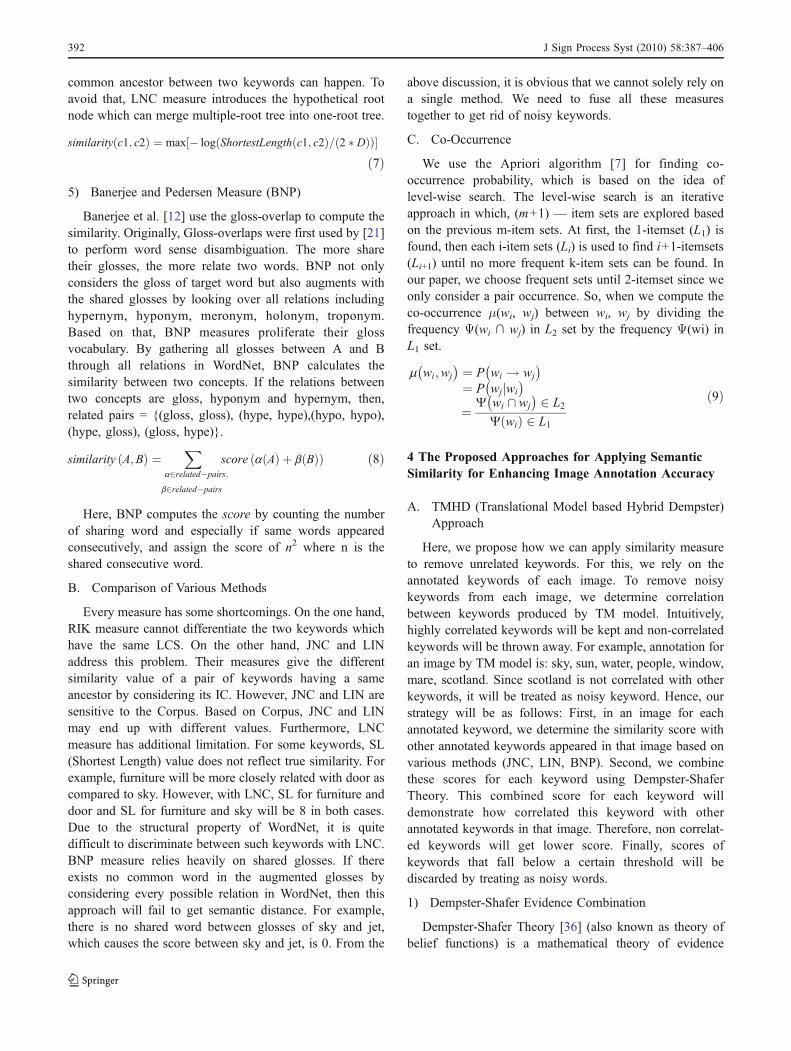
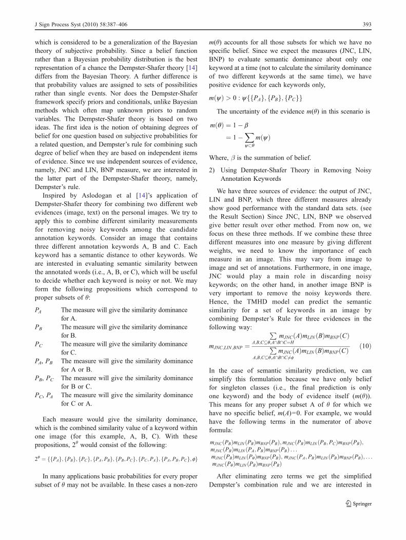
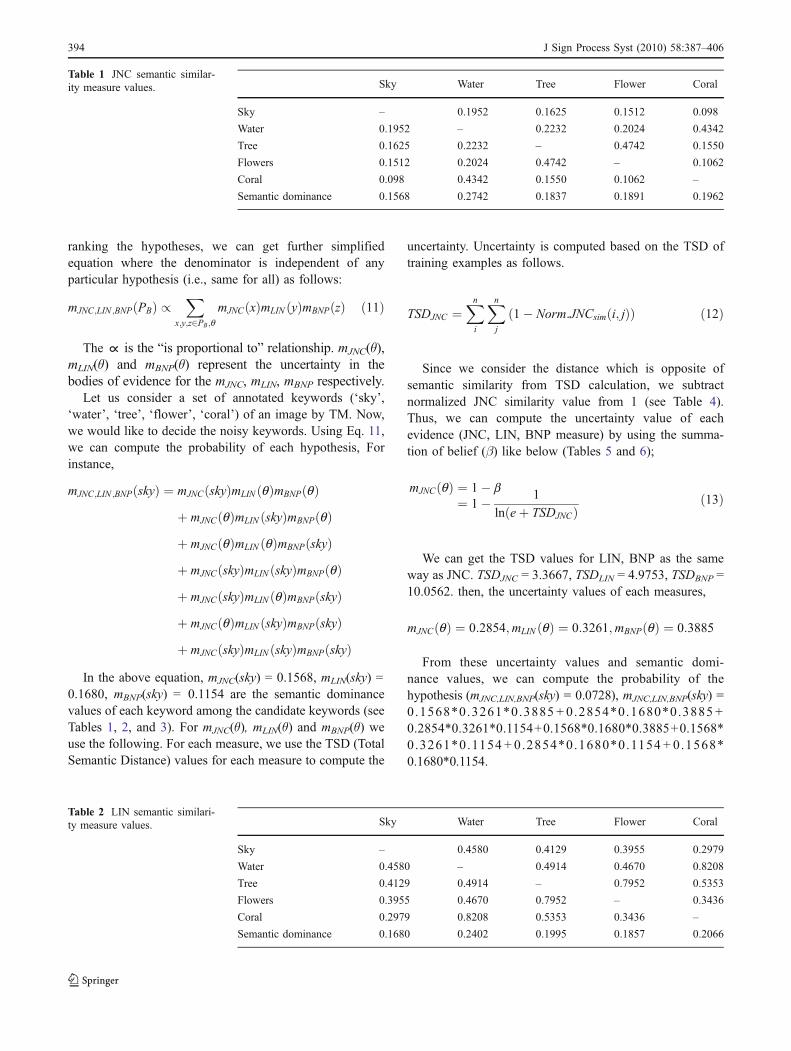
Let us consider a set of annotated keywords (‘sky’,‘water’, ‘tree’, ‘flower’, ‘coral’) of an image by TM. Now,we would like to decide the noisy keywords. Using Eq. 11,we can compute the probability of each hypothesis, Forinstance,

mJNC;LIN ;BNP skyð Þ ¼ mJNC skyð ÞmLIN qð ÞmBNP qð Þþ mJNC qð ÞmLIN skyð ÞmBNP qð Þþ mJNC qð ÞmLIN qð ÞmBNP skyð Þþ mJNC skyð ÞmLIN skyð ÞmBNP qð Þþ mJNC skyð ÞmLIN qð ÞmBNP skyð Þþ mJNC qð ÞmLIN skyð ÞmBNP skyð Þþ mJNC skyð ÞmLIN skyð ÞmBNP skyð Þ

In the above equation, mJNC(sky) = 0.1568, mLIN(sky) =0.1680, mBNP(sky) = 0.1154 are the semantic dominancevalues of each keyword among the candidate keywords (seeTables 1, 2, and 3). For mJNC(θ), mLIN(θ) and mBNP(θ) weuse the following. For each measure, we use the TSD (TotalSemantic Distance) values for each measure to compute the

uncertainty. Uncertainty is computed based on the TSD oftraining examples as follows.

TSDJNC ¼Xn

i

Xn

j

1� Norm:JNCsim i; jð Þð Þ ð12Þ

Since we consider the distance which is opposite ofsemantic similarity from TSD calculation, we subtractnormalized JNC similarity value from 1 (see Table 4).Thus, we can compute the uncertainty value of eachevidence (JNC, LIN, BNP measure) by using the summa-tion of belief (β) like below (Tables 5 and 6);

mJNC qð Þ ¼ 1� b¼ 1� 1

ln eþ TSDJNCð Þð13Þ

We can get the TSD values for LIN, BNP as the sameway as JNC. TSDJNC = 3.3667, TSDLIN = 4.9753, TSDBNP =10.0562. then, the uncertainty values of each measures,

mJNC qð Þ ¼ 0:2854;mLIN qð Þ ¼ 0:3261;mBNP qð Þ ¼ 0:3885

From these uncertainty values and semantic domi-nance values, we can compute the probability of thehypothesis (mJNC,LIN,BNP(sky) = 0.0728), mJNC,LIN,BNP(sky) =0.1568*0.3261*0.3885 + 0.2854*0.1680*0.3885 +0.2854*0.3261*0.1154+0.1568*0.1680*0.3885+0.1568*0.3261*0.1154 + 0.2854*0.1680*0.1154 + 0.1568*0.1680*0.1154.

Sky Water Tree Flower Coral

Sky – 0.1952 0.1625 0.1512 0.098

Water 0.1952 – 0.2232 0.2024 0.4342

Tree 0.1625 0.2232 – 0.4742 0.1550

Flowers 0.1512 0.2024 0.4742 – 0.1062

Coral 0.098 0.4342 0.1550 0.1062 –

Semantic dominance 0.1568 0.2742 0.1837 0.1891 0.1962

Table 1 JNC semantic similar-ity measure values.


Sky – 0.4580 0.4129 0.3955 0.2979

Water 0.4580 – 0.4914 0.4670 0.8208

Tree 0.4129 0.4914 – 0.7952 0.5353

Flowers 0.3955 0.4670 0.7952 – 0.3436

Coral 0.2979 0.8208 0.5353 0.3436 –


Table 2 LIN semantic similari-ty measure values.


Like this, we can do the same computation for othercandidate keywords. We can get the final combinationresult from the simplified equation.

mJNC;LIN ;BNP skyð Þ ¼ 0:0728P

mJNC;LIN ;BNP waterð Þ ¼ 0:1719P

mJNC;LIN ;BNP treeð Þ ¼ 0:0945P

mJNC;LIN ;BNP flowerð Þ ¼ 0:1215P

mJNC;LIN ;BNP coralð Þ ¼ 0:1978P

Since the denominator is the same, and we are onlyinterested in the ranking, we can simplify it by thefollowing way.

mJNC,LIN,BNP(sky) = 0.1303, mJNC,LIN,BNP(water) = 0.3077,mJNC,LIN,BNP(tree) = 0.1692, mJNC,LIN,BNP(flower) = 0.2175,mJNC,LIN,BNP(coral) = 0.1751. Then, we can remove key-words that below a certain threshold value (for this image,0.17). Then, ‘tree’, ‘sky’ will be treated as noisy keywordand the remaining annotation words are ‘water’, ‘flower’,‘coral’ (Fig. 4).

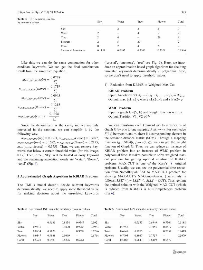
5 Approximated Graph Algorithm in KBIAR Problem

The TMHD model doesn’t decide relevant keywordsdeterministically; we need to apply some threshold valuefor making decision about the un-related keywords

(‘crystal’, ‘anemone’, ‘reef’-see Fig. 5). Here, we intro-duce an approximation based graph algorithm for decidingunrelated keywords deterministically in polynomial time,so we don’t need to apply threshold values.

1) Reduction from KBIAR to Weighted Max-Cut

KBIAR ProblemInput: Annotated Set Ak ¼ ak1; ak2; . . . ; aknf g; SDMn�nOutput: max {s1, s2}, where s1,s2⊂Ak and s1∩s2=ϕ

WMC ProblemInput: a graph G=(V, E) and weight function w (i, j)Output: Partition V1, V2 of V

We can transform each keyword aki to a vertex vi ofGraph G by one to one mapping f(:aki→vi). For each edgeE(i, j) between vi and vj, there is a corresponding element inthe semantic distance matrix (SDM). Through a mappingfunction (g : SDM(i, j)→w(i, j)), we can get the weightfunction of Graph G. Thus, we can reduce an instance ofKBIAR problem into an instance of WMC problem inpolynomial time. It makes possible to solve weighted max-cut problem for getting optimal solution of KBIARproblem. MAX-CUT is one of the Karp’s [8] originalproblem. Usually, we can see the polynomial-time reduc-tion from NotAllEqual-3SAT to MAX-CUT problem forshowing MAX-CUT’s NP-Completeness. (Transitivity isfollows; 3SAT �p 6¼ 3SAT �p MAX � CUT ). Thus, gettingthe optimal solution with the Weighted MAX-CUT (whichis reduced from KBIAR) is NP-Completeness problem(Fig 6).


Sky – 2 2 2 0

Water 2 – 4 5 2

Tree 2 4 – 29 4

Flowers 2 5 29 – 2

Coral 0 2 4 2 –


Table 3 BNP semantic similar-ity measure values.

Table 4 Normalized JNC semantic similarity measure values.


Sky – 0.9535 0.8834 0.9347 0.5921

Water 0.9535 – 0.9820 0.9968 0.6983

Tree 0.8834 0.9820 – 0.9699 0.6296

Flowers 0.9347 0.9968 0.9699 – 0.6764

Coral 0.5921 0.6983 0.6296 0.6764 –

Table 5 Normalized LIN semantic similarity measure values.


Sky – 0.7553 0.6949 0.7364 0.5188

Water 0.7553 – 0.7955 0.8417 0.9843

Tree 0.6949 0.7955 – 0.7757 0.8419

Flowers 0.7905 0.8967 0.7757 – 0.5679

Coral 0.5188 0.9843 0.8419 0.5679 –


2) Optimal Solution of WMC Problem

Let us represent WMC problem as integer quadraticproblem (WMC-IQP);

Maximize

1

2

Xn

j¼1

Xj�1

i¼1w i; jð Þ 1� mi � mj

� � ð14Þ

Subject to mi 2 �1; 1f g; 1 � i � n; where n ¼ Vj j

mi is the membership binary values, in that, if adjacentvertices ma, mb are belong to different set V1, V2respectively by the current cut, then the membershipvalues for each ma, mb will be different (−1,1). So, 1−ma×mb value is 2, if ma, mb are in same set, then 1−ma × mb

value is 0, then its weight value doesn’t count as the totalweight of a cut instance. The instance that makes themaximum total weight of cut would be optimal partition V1,V2 of the graph. If we find the maximum cut in non-

deterministic way, then we can guess an assignment of eachvertex’s set and compute the optimal value of the above IQP(Integer Quadratic Problem). To do this thoroughly (namely,check with every possible combinations), we need exponen-tial amount of time (2n). To find max-cut in polynomial time,we need an approximation scheme for MAX-CUT problem.

3) Randomized Approximation WMC (Weighted Max-Cut) in KBIAR

Our work is based on Goeman [9]’s randomized 0.87856approximation scheme for finding maximum-cut that isconstructed with each image’s candidate annotation key-words and semantic similarity between those words.Goeman et al. [9] showed the way of relaxing frominteger quadratic problem to semi-definite programming byincreasing the dimensions of membership value mi from 1to n dimensions and constructing a matrix M such that mi,j

is corresponding to each inner product mi·mj. As a step ofrelaxation, it relaxes membership variable conditions;

1� dimensional variable of unit norm

!Relaxation 2� dimensional vector space of unit norm

Let us define WMC 2-relaxation problem (WMC-2VQP);

Maximize1

2

Xn

j¼1

Xj�i

i¼1w i; jð Þ 1� mi � mj

� �

Subject to mi � mj mi 2 R2; 1 � i � n; where n ¼ Vj jIf we have a feasible solution of WMC-IQP, then it also

can be easily a feasible solution to WMC-2IQP since 2-

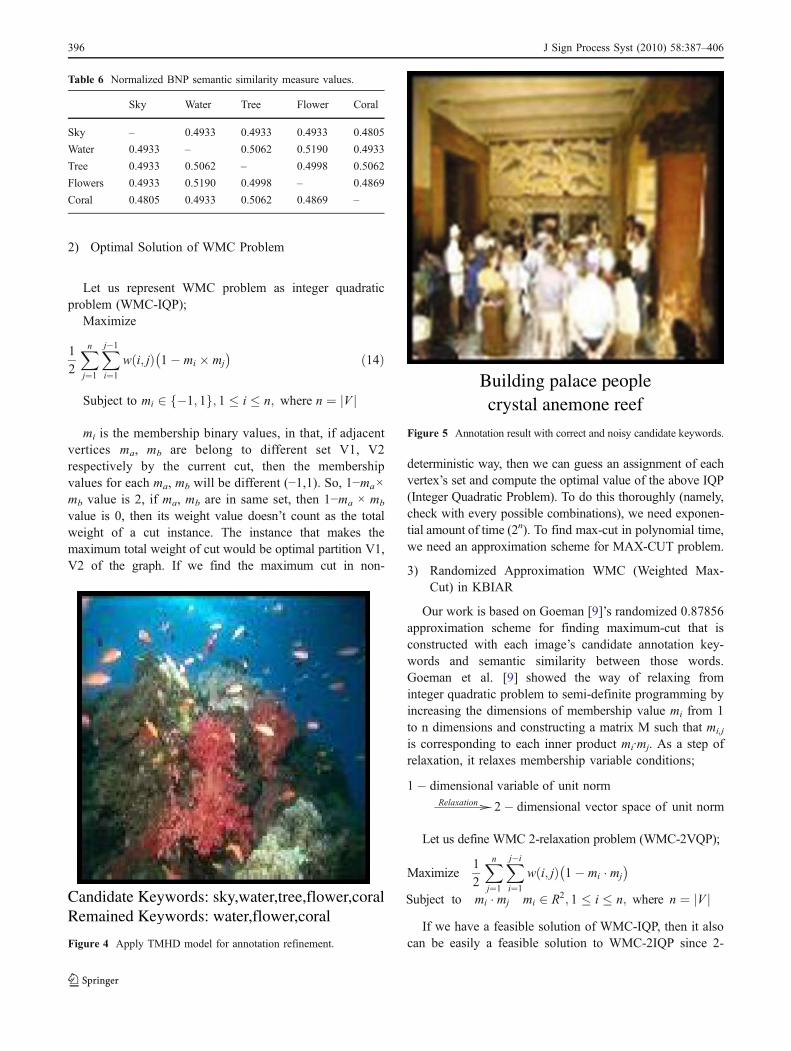
Building palace peoplecrystal anemone reef

Figure 5 Annotation result with correct and noisy candidate keywords.

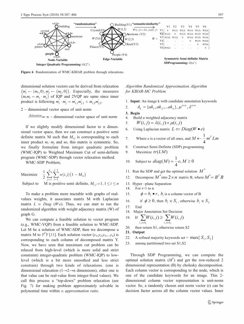
Candidate Keywords: sky,water,tree,flower,coralRemained Keywords: water,flower,coral

Figure 4 Apply TMHD model for annotation refinement.

Table 6 Normalized BNP semantic similarity measure values.


Sky – 0.4933 0.4933 0.4933 0.4805

Water 0.4933 – 0.5062 0.5190 0.4933

Tree 0.4933 0.5062 – 0.4998 0.5062

Flowers 0.4933 0.5190 0.4998 – 0.4869

Coral 0.4805 0.4933 0.5062 0.4869 –


dimensional solution vectors can be derived from relaxation�m0i mi; 0ð Þ;m0j

�mj; 0

��. Especially, the measures�

mimj ¼ m0i � m

0j

�of IQP and 2VQP are same since inner

product is following m0i � m

0j ¼ m

0i;1m

0j;1 þ m

0

i;2m0j;2.

2� dimensional vector space of unit norm

!Relaxation n� dimensional vector space of unit norm

If we slightly modify dimensional factor to n dimen-sional vector space, then we can construct a positive semidefinite matrix M such that Mi,j is corresponding to eachinner product mi • mj and so, this matrix is symmetric. So,we finally formulate from integer quadratic problem(WMC-IQP) to Weighted Maximum Cut of semi-definiteprogram (WMC-SDP) through vector relaxation method.

WMC-SDP Problem;

Maximize1

2

Xn

j¼1

Xj�1

i¼1w i; jð Þ 1�Mi;j

� �

Subject to M is positive semi�definite; Mi; j¼1; 1� i � n

To make a problem more tractable with graphs of real-values weights, it associates matrix M with Laplacianmatrix L ⇐ Diag (W·e). Thus, we can start to run therandomized algorithm with weight adjacency matrix (W) ofgraph G.

We can compute a feasible solution to vector program(e.g., WMC-VQP) from a feasible solution to WMC-SDP.Let M be a solution of WMC-SDP, then we decompose amatrix M to YTY [11]. Each solution vector (y1,y2,y3,...yn) iscorresponding to each column of decomposed matrix Y.Now, we have seen that maximum cut problem can berelaxed from high-level (which is more solid and strictconstraint) integer-quadratic problem (WMC-IQP) to low-level (which is a bit more smoothed and less strictconstrain) through two kinds of relaxations. (one isdimensional relaxation (1→2→n dimensions), other one isthat value can be real-value from integer-fixed values). Wecall this process a “top-down” problem relaxation (seeFig. 7) for making problem approximately solvable inpolynomial time within α approximation ratio.

Algorithm Randomized Approximation Algorithmfor KBIAR-MC Problem

Through SDP Programming, we can compute theoptimal solution matrix (M*) and get the row-reduced 2dimensional representation (B) by cholesky decomposition.Each column vector is corresponding to the node, which isone of the candidate keywords for an image. This 2-dimensional column vector representation is unit-normvector. So, a randomly chosen unit norm vector (r) can bedecision factor across all the column vector values. Inner

building< 1,1>

< 1 1> < 1 1>crystal

“randomization” Building(V1)

A (V2)Crystal(V6)

)62()52()42()32(0)12(

)6,1()5,1()4,1()3,1()2,1(0

WWWWW

WWWWW

V1 V2 V3 V4 V5 V6V1V2

“semanticsimilarity”

)2,1(W ),(),(),( jijijiW< 1,1> < , >

< 1,1>< 1,1>

anemone

reef

people

palace

Anemone

Reef(V3)

( )

Palace(V5) 0........)1,6(

)6,5(0........

)6,4()5,4(0......

)6,3()5,3()4,3(0)2,3()1,3(

,,,,,

W

W

WW

WWWWW

V2V3V4V5V6

)3,2(W)6,5(W W

< 1,1>people People V4

Node Variable Edge Variable Symmetric Semi definite Matrix

Integer Quadratic Programming: )2( nO SDProgramming: )( 3nO

Figure 6 Randomization of WMC-KBIAR problem through relaxations.


product result (ϕ=bi · r) can separate each node into twosets (Fig. 8). To decide a major set, we compare thesummation value of semantic similarity (see Line 19)among all candidate words assigned to a set.

4) Complexity Analysis

Basically, MAX-CUT problem belongs to NP-completeproblem, which is one of the Karp’s [8] original problem.

Usually, we can see the polynomial-time reduction fromNAE-3SAT to MAX-CUT problem for showing MAX-CUT’s NP-Completeness. In that, if we find the maximumcut in non-deterministic way, then we can guess anassignment of each vertex’s set and compute the numberof edges which are cross the two set. To do this thoroughly(namely, check with every possible combinations), we needexponential amount of time (2n). To find max-cut inpolynomial time, we need an approximation scheme forMAX-CUT problem. In the Approximation Class, Vega etal. [38] showed that dense weighted max-cut and metricmax-cut can have a polynomial time approximation scheme(namely, PTAS) ([39] demonstrated a reduction from metricmax-cut to dense max-cut problem). However, if we haveto deal with general max-cut problem, then it is belong toAPX-Complete class. ([40]. - MAX-3SAT ≥AP MAX-2SAT≥AP MAX-NAE3SAT ≥AP MAX-CUT). Crescenzi et al.[41] claim that non-weighted version of MAX-CUT also ashard as weighted version of MAX-CUT problem byshowing AP reduction from weighted MAX-CUT toMAX-CUT. After Sahni and Gonzalez [42] showed thetrivial 1/2 approximation algorithm, there was no realprogress until the Goemans et al. [9]’s a randomizedapproximation approach appear. Our work is based onGoeman’s randomized approximation scheme for findingmaximum-cut that is constructed with each image’scandidate annotation keywords and semantic similarity

Figure 7 Flow of the Randomized Approximation Scheme using 2-way approaches (Top-down-“relaxation” and Bottom-up-“solving”).

1959.02189.05124.00121.00686.00

9806.09757.08586.09999.09976.01B

}3,2,1{1 bbbS 0,1, rbSbi ii

}6,5,4{2 bbbS 0,2, rbSbj jj

Figure 8 2-dimensional mapping into the random-hyper plane for thecut decision.


between those words. This approximation algorithm can getthe maximal cut which is 0.87856 times the optimalsolution [9]. In terms of running time, after randomizinginto semi-definite matrix, it uses semi-definite programming(it needs O

ffiffiffinp

logW þ log 1="ð Þð Þ iterations, each iterationcan be implemented in O(n3) time. After that, it uses anincomplete cholesky decomposition process, which takesO(n3). Consequently, if we use this randomized approxima-tion algorithm, then it takes O c

ffiffiffinp

n3ð Þ and get the maximalcut that has a 0.87856 times measure of optimal solution.

6 Experiment and Results

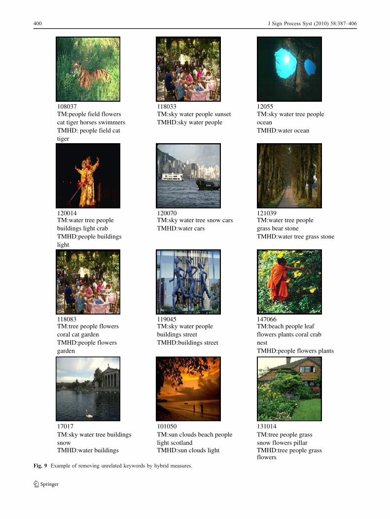
In this section, first, we present the set up of our experi-ments. Next, we compare our results with other techniques.We use a data set that contains 5,000 images from 50 StockPhoto Cds ([13]). Each Cd contains 100 images on thesame topic. We use 4,500 images as training set and theremaining 500 images as testing set. The image segmenta-tion algorithm is the normalized cut [30]. Each image isrepresented as 30 dimensional vector, which corresponds to30 low-level features. The vocabulary contains 374 differ-ent keywords. We reprocess the data set as follows. First,we cluster a total of 42,379 image objects from 4,500training images into 500 blobs using K-means algorithmand weighted selection method. Next, we apply EMalgorithm to annotate keywords for each images automat-ically. This will be known as TM model. Finally, we applyhybrid measures (TMHD) to get rid of some noisyannotated keywords. In Fig. 9, we demonstrate the powerof the approach, THMD over TM. For example, one of theexample image (108037) includes very unrelated keywords(horse, swimmers) which could make the CBIR systemmisunderstand the image. After post processing, the imagedoes not only excludes those noisy keywords, but alsokeeps ‘cat’ as annotation. However, ‘cat’ does not make bigsemantic difference for understanding this image. Let usconsider the image with identifier 147066 (the last image).This image has a set of noisy keywords (beach, coral, crab,nest). We can see TM generates these noisy keywords,while TMHD discards all these noisy/irrelevant keywordsand keeps only relevant ones. However, if we consider thesecond image (identifier 17017), in Fig. 9, TMHD discardsthe irrelevant keyword ‘sky’ along with the relevantkeywords ‘tree’. Therefore, TMHD discards occasionallysome relevant keywords.

1) Comparison of Various Measures

Here we would like to demonstrate the superiority ofTMHD over various methods and using different measures.We report the results using two sets and based on two

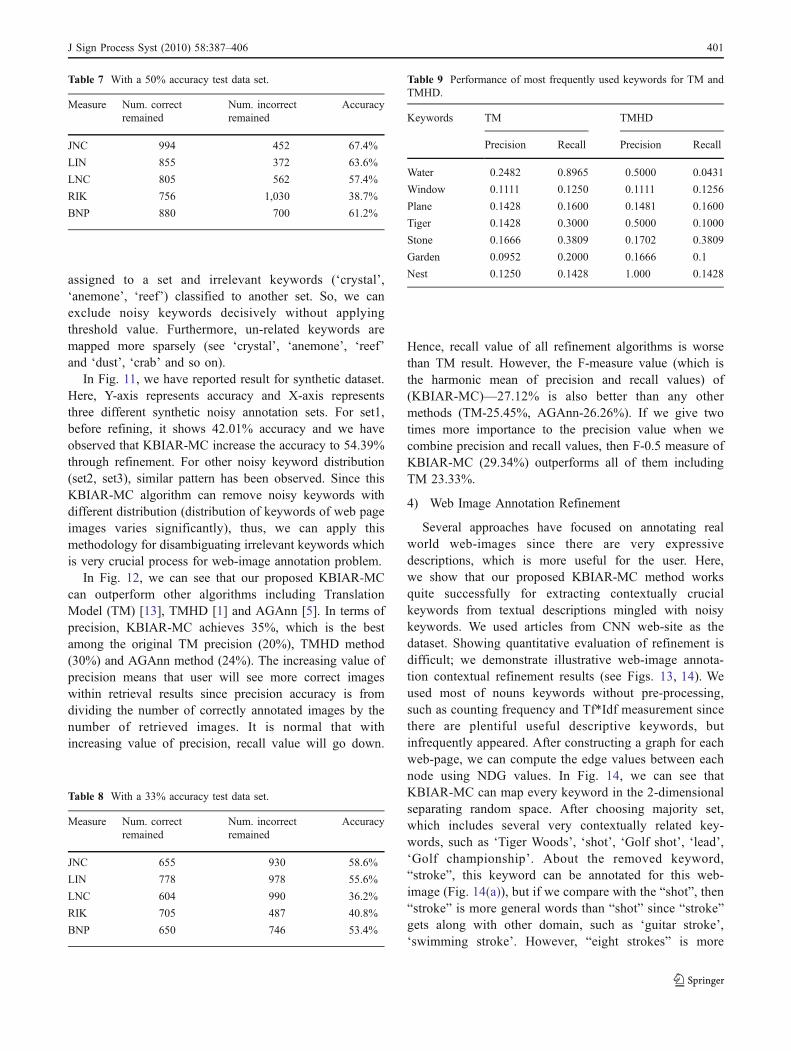
accuracy levels (50% and 33%). We prepare the two sets asfollows. Initially, we select 500 images along with sixmanually annotated correct keywords. For the first set, weprepare dataset with 50% accuracy in keyword annotation,which means that the ratio of correct and incorrectkeywords of an image is 0.5:0.5. To achieve this, weremove three correct keywords from an image and insertthree noisy keywords randomly. Similarly, we construct thesecond dataset with 33% accuracy. In Table 7, given thefirst dataset with 50% accuracy, JNC improves the accuracyto 67.4%. Here, JNC measure chooses 994 correct key-words out of 1,500 keywords and removes 1,058 incorrectkeywords from 1,500 keywords. Furthermore, notice thatJNC, LIN, and BNP measures outperform RIK and LNCmeasures. In Table 8, with dataset 2 (accuracy 33%),accuracy of JNC, LIN, BNP measures are still greater than50% even with 67% noisy keywords in the images. Thisdemonstrates the power of the semantic similarity meas-ures. From these two tables, JNC, LIN and BNP are thebest measures regardless of the distribution of noisykeywords. Therefore, in TMHD, we combine all thesethree measures (JNC, LIN and BNP), and ignore the othertwo (RIK and LNC).

2) Comparison of TMHD with TM

Here we report results based on most frequently usedkeywords for TMHD and TM. Recall that TMHD considershybrid measures. For the keyword ‘nest’, we observe thatthe precision of TMHD (100%) is substantially higher thanprecision of TM (12.5%), on the other hand, the recall is thesame in both cases (14.28%). This happens due to the removalof only noisy keywords and not discarding relevant keywords(i.e., recall is the same). For all keywords, precision of TMHDhas increased as compared to TM at some extent. Note thatwhen precision increases, recall drops. However, here weobserve that, except for the keywords, ‘water’, ‘tiger’, and‘garden’, recall is the same in both models. On average, theprecision values of TM and TMHD models are 14.21%, and33.11% respectively. This number demonstrates that TMHDis 56.87% better than TM (Tables 7, 8 and 9).

3) Performance Analysis ofMax-Cut Refinement Algorithm

For implementation of randomized approximation ofweight-max-cut algorithm, we utilized the SDTP3 Matlabsoftware [10, 35] for computing semi-definite programmingpart in the whole approximation algorithm. To see the effectof refinement in the various distribution of noisy keywords,we use synthetic annotation data where we vary distributionof noisy keywords. However, when report, precision, recalland F-measure, we use original dataset. In Fig. 10, we cansee the 2d-mapping result examples of coral data set. Therelated keywords (‘building’, ‘palace’, ‘people’) has been


TM:beach people leaf147066

TMHD:buildings streetbuildings streetTM:sky water people119045

gardenTMHD:people flowers coral cat gardenTM:tree people flowers118083

TMHD:water tree grass stonegrass bear stoneTM:water tree people121039

flowers plants coral crab

flowersTMHD:tree people grasssnow flowers pillarTM:tree people grass131014

TMHD:sun clouds lightlight scotlandTM:sun clouds beach people101050

TMHD:water buildingssnowTM:sky water tree buildings17017

TMHD:people flowers plantsnest

TMHD:water cars

cat tiger horses swimmersTM:people field flowers108037

TMHD: people field cat

TM:sky water tree snow cars120070

lightTMHD:people buildings buildings light crabTM:water tree people120014

TMHD:water oceanoceanTM:sky water tree people12055

TMHD:sky water peopleTM:sky water people sunset118033

tiger

Fig. 9 Example of removing unrelated keywords by hybrid measures.


assigned to a set and irrelevant keywords (‘crystal’,‘anemone’, ‘reef’) classified to another set. So, we canexclude noisy keywords decisively without applyingthreshold value. Furthermore, un-related keywords aremapped more sparsely (see ‘crystal’, ‘anemone’, ‘reef’and ‘dust’, ‘crab’ and so on).

In Fig. 11, we have reported result for synthetic dataset.Here, Y-axis represents accuracy and X-axis representsthree different synthetic noisy annotation sets. For set1,before refining, it shows 42.01% accuracy and we haveobserved that KBIAR-MC increase the accuracy to 54.39%through refinement. For other noisy keyword distribution(set2, set3), similar pattern has been observed. Since thisKBIAR-MC algorithm can remove noisy keywords withdifferent distribution (distribution of keywords of web pageimages varies significantly), thus, we can apply thismethodology for disambiguating irrelevant keywords whichis very crucial process for web-image annotation problem.

In Fig. 12, we can see that our proposed KBIAR-MCcan outperform other algorithms including TranslationModel (TM) [13], TMHD [1] and AGAnn [5]. In terms ofprecision, KBIAR-MC achieves 35%, which is the bestamong the original TM precision (20%), TMHD method(30%) and AGAnn method (24%). The increasing value ofprecision means that user will see more correct imageswithin retrieval results since precision accuracy is fromdividing the number of correctly annotated images by thenumber of retrieved images. It is normal that withincreasing value of precision, recall value will go down.

Hence, recall value of all refinement algorithms is worsethan TM result. However, the F-measure value (which isthe harmonic mean of precision and recall values) of(KBIAR-MC)—27.12% is also better than any othermethods (TM-25.45%, AGAnn-26.26%). If we give twotimes more importance to the precision value when wecombine precision and recall values, then F-0.5 measure ofKBIAR-MC (29.34%) outperforms all of them includingTM 23.33%.

4) Web Image Annotation Refinement

Several approaches have focused on annotating realworld web-images since there are very expressivedescriptions, which is more useful for the user. Here,we show that our proposed KBIAR-MC method worksquite successfully for extracting contextually crucialkeywords from textual descriptions mingled with noisykeywords. We used articles from CNN web-site as thedataset. Showing quantitative evaluation of refinement isdifficult; we demonstrate illustrative web-image annota-tion contextual refinement results (see Figs. 13, 14). Weused most of nouns keywords without pre-processing,such as counting frequency and Tf*Idf measurement sincethere are plentiful useful descriptive keywords, butinfrequently appeared. After constructing a graph for eachweb-page, we can compute the edge values between eachnode using NDG values. In Fig. 14, we can see thatKBIAR-MC can map every keyword in the 2-dimensionalseparating random space. After choosing majority set,which includes several very contextually related key-words, such as ‘Tiger Woods’, ‘shot’, ‘Golf shot’, ‘lead’,‘Golf championship’. About the removed keyword,“stroke”, this keyword can be annotated for this web-image (Fig. 14(a)), but if we compare with the “shot”, then“stroke” is more general words than “shot” since “stroke”gets along with other domain, such as ‘guitar stroke’,‘swimming stroke’. However, “eight strokes” is more

Table 9 Performance of most frequently used keywords for TM andTMHD.

Keywords TM TMHD

Precision Recall Precision Recall

Water 0.2482 0.8965 0.5000 0.0431

Window 0.1111 0.1250 0.1111 0.1256

Plane 0.1428 0.1600 0.1481 0.1600

Tiger 0.1428 0.3000 0.5000 0.1000

Stone 0.1666 0.3809 0.1702 0.3809

Garden 0.0952 0.2000 0.1666 0.1

Nest 0.1250 0.1428 1.000 0.1428

Table 7 With a 50% accuracy test data set.

Measure Num. correctremained

Num. incorrectremained

Accuracy

JNC 994 452 67.4%

LIN 855 372 63.6%

LNC 805 562 57.4%

RIK 756 1,030 38.7%

BNP 880 700 61.2%

Table 8 With a 33% accuracy test data set.

Measure Num. correctremained

Num. incorrectremained

Accuracy

JNC 655 930 58.6%

LIN 778 978 55.6%

LNC 604 990 36.2%

RIK 705 487 40.8%

BNP 650 746 53.4%


close to “shot” since “eight stroke” expressions usuallyused in Golf Domain. This is quite good example ofKBIAR-MC can semantically group contextual similarwords as the neighbors in the 2-dimensional separatingrandom space. KBIAR-MC can also refine keywords

iteratively. Among the selected words, which are quiteclosely mapped in Fig. 14(b) When we run KBIAR-MCagain with remaining keywords, then we can removeadditionally unrelated keywords (‘town’, ‘terror’, ‘terror-

building,palace,peoplecrystal,anemone,reef

Refined"Annotation:building,palace,people

colstume,people,streetvillage,sphinx,light,dust,crab

Refined"Annotation:costume,people,street,village

Figure 10 Result examples ofrandom space separation frommax-cut refinement algorithm.

Set1 Set2 Set30

0.2

0.4

0.6

0.8

1

Synthetic Noisy DataSet

Acc

urac

y

max–cut refinementun–refined noisy set

Figure 11 Accuracy enhancement through weighted max-cut refine-ment with synthetic noisy dataset.

TM TMHD AGAnn KBIARMC0

0.1

0.2

0.3

0.4

Acc

urac

y

PrecisionRecall

F–1 MeasureF–0.5 Measure

Figure 12 Refrinement performance comparison between severalapproaches.


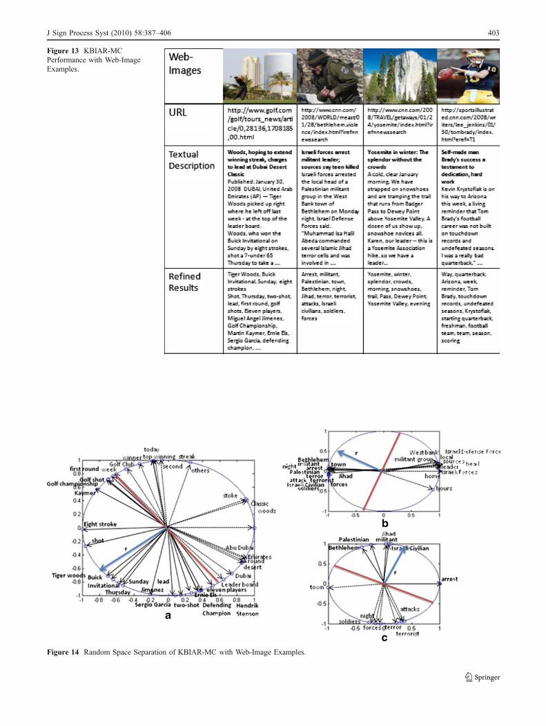
Figure 13 KBIAR-MCPerformance with Web-ImageExamples.

Figure 14 Random Space Separation of KBIAR-MC with Web-Image Examples.


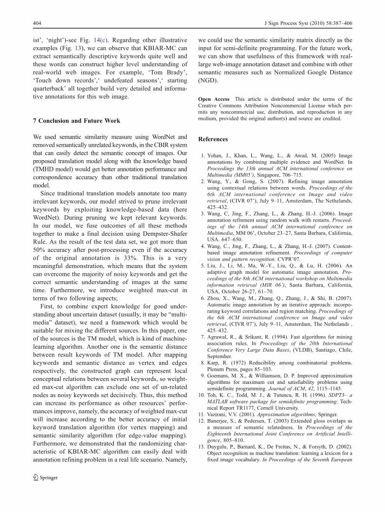
ist’, ‘night’)-see Fig. 14(c). Regarding other illustrativeexamples (Fig. 13), we can observe that KBIAR-MC canextract semantically descriptive keywords quite well andthese words can construct higher level understanding ofreal-world web images. For example, ‘Tom Brady’,‘Touch down records’,‘ undefeated seasons’,‘ startingquarterback’ all together build very detailed and informa-tive annotations for this web image.

7 Conclusion and Future Work

We used semantic similarity measure using WordNet andremoved semantically unrelated keywords, in the CBIR systemthat can easily detect the semantic concept of images. Ourproposed translation model along with the knowledge based(TMHD model) would get better annotation performance andcorrespondence accuracy than other traditional translationmodel.

Since traditional translation models annotate too manyirrelevant keywords, our model strived to prune irrelevantkeywords by exploiting knowledge-based data (hereWordNet). During pruning we kept relevant keywords.In our model, we fuse outcomes of all these methodstogether to make a final decision using Dempster-ShaferRule. As the result of the test data set, we got more than50% accuracy after post-processing even if the accuracyof the original annotation is 33%. This is a verymeaningful demonstration, which means that the systemcan overcome the majority of noisy keywords and get thecorrect semantic understanding of images at the sametime. Furthermore, we introduce weighted max-cut interms of two following aspects;

First, to combine expert knowledge for good under-standing about uncertain dataset (usually, it may be “multi-media” dataset), we need a framework which would besuitable for mixing the different sources. In this paper, oneof the sources is the TM model, which is kind of machine-learning algorithm. Another one is the semantic distancebetween result keywords of TM model. After mappingkeywords and semantic distance as vertex and edgesrespectively, the constructed graph can represent localconceptual relations between several keywords, so weight-ed max-cut algorithm can exclude one set of un-relatednodes as noisy keywords set decisively. Thus, this methodcan increase its performance as other resources’ perfor-mances improve, namely, the accuracy of weighted max-cutwill increase according to the better accuracy of initialkeyword translation algorithm (for vertex mapping) andsemantic similarity algorithm (for edge-value mapping).Furthermore, we demonstrated that the randomizing char-acteristic of KBIAR-MC algorithm can easily deal withannotation refining problem in a real life scenario. Namely,

we could use the semantic similarity matrix directly as theinput for semi-definite programming. For the future work,we can show that usefulness of this framework with real-large web-image annotation dataset and combine with othersemantic measures such as Normalized Google Distance(NGD).

Open Access This article is distributed under the terms of theCreative Commons Attribution Noncommercial License which per-mits any noncommercial use, distribution, and reproduction in anymedium, provided the original author(s) and source are credited.

References

1. Yohan, J., Khan, L., Wang, L., & Awad, M. (2005) Imageannotations by combining multiple evidence and WordNet. InProceedings the 13th annual ACM international conference onMultimedia (MM05’), Singapore, 706–715.

2. Wang, Y., & Gong, S. (2007). Refining image annotationusing contextual relations between words. Proceedings of the6th ACM international conference on Image and videoretrieval, (CIVR 07’), July 9–11, Amsterdam, The Nethelands,425–432.

3. Wang, C, Jing, F., Zhang, L., & Zhang, H.-J. (2006). Imageannotation refinment using random walk with restarts. Proceed-ings of the 14th annual ACM international conference onMultimedia, MM 06’, October 23–27, Santa Barbara, California,USA. 647–650.

4. Wang, C., Jing, F., Zhang, L., & Zhang, H.-J. (2007). Content-based image annotation refinement. Proceedings of computervision and pattern recognition. CVPR’07.

5. Liu, J., Li, M., Ma, W.-Y., Liu, Q., & Lu, H. (2006). Anadaptive graph model for automatic image annotation. Pro-ceedings of the 8th ACM international workshop on Multimediainformation retrieval (MIR 06’), Santa Barbara, California,USA, October 26-27, 61–70.

6. Zhou, X., Wang, M., Zhang, Q., Zhang, J., & Shi, B. (2007).Automatic image annotation by an iterative approach: incorpo-rating keyword correlations and region matching. Proceedings ofthe 6th ACM international conference on Image and videoretrieval, (CIVR 07’), July 9–11, Amsterdam, The Nethelands ,425–432.

7. Agrawal, R., & Srikant, R. (1994). Fast algorithms for miningassociation rules. In Proceedings of the 20th InternationalConference Very Large Data Bases, (VLDB), Santiago, Chile,September.

8. Karp, R. (1972) Reducibility among combinatorial problems.Plenum Press, pages 85–103.

9. Goemans, M. X., & Williamson, D. P. Improved approximationalgorithms for maximum cut and satisfiability problems usingsemidefinite programming. Journal of ACM, 42, 1115–1145.

10. Toh, K. C., Todd, M. J., & Tutuncu, R. H. (1996). SDPT3– aMATLAB software package for semidefinite programming. Tech-nical Report TR1177, Cornell University.

11. Vazirani, V.V. (2001). Approximation algorithms, Springer.12. Banerjee, S., & Pedersen, T. (2003) Extended gloss overlaps as

a measure of semantic relatedness. In Proceedings of theEighteenth International Joint Conference on Artificial Intelli-gence, 805–810.

13. Duygulu, P., Barnard, K., De Freitas, N., & Forsyth, D. (2002).Object recognition as machine translation: learning a lexicon for afixed image vocabulary. In Proceedings of the Seventh European


Conference on Computer Vision (ECCV) Part IV, Copenhagen,Denmark, 97–112.

14. Aslandogan, Y. A. & Yu, C.-T. (2000). Diogenes: A web searchagent for content based indexing of personal images. InProceedings of ACM SIGIR 2000, Athens, Greece, pages 481–482.

15. Jeon, J., Lavrenko, V., & Manmatha, R. (2003). Automatic imageannotation and retrieval using cross-media relevance models.Proceedings of the 26th Annual International ACM SIGIRConference ,Toronto, Canada, 119–126.

16. Jiang, J., & Conrath, D. (1997). Semantic similarity based on corpusstatistics and lexical taxonomy. In Procedeeings on InternationalConference on Research in Computational Linguistics, Taiwan.

17. Kang, F., Jin, R., & Chai, J. Y. (2004). Regularizing translationmodels for better automatic image annotation. In Proceedings ofThe Thirteenth Conference on Information and KnowledgeManagement, 2004, Washington D. C., USA, Nov. 8-13, 350-359.

18. Lavrenko, V. Feng, S. L., & Manmatha (2004). Statistical modelsfor automatic video annotation and retrieval. InternationalConference on Acoustics, Speech and Signal Processing,(ICASSP) Montreal, QC, Canada, 17–21.

19. Li, J., & Wang, J. Z. Automatic linguistic indexing of pictures bya statistical modeling approach. IEEE Transaction on PatternAnalysis and Machine Intelligence, 25(9), 1075–1088.

20. Leacock, C., & Chodorow, M. (1998). Combining local context andWordNet similarity for word sense identification. WordNet:Anelectronic lexical database. In C. Fellbaum (Ed.), MIT Press, 265–283.

21. Lesk, M. (1986). Automatic sense disambiguation machinereadable dictionaries: How to tell a pine cone from an ice creamcone. In Proceedings of the 5th annual international conference onSystems documentation, Toronto, Ontario, Canada. ACM Press,NewYork, NY, USA, 24–26.

22. Lin, D. (1997). Using syntactic dependency as a local context toresolve word sense ambiguity. In Proceedings of the 35th AnnualMeeting of the Association for Computational Linguistics.Madrid, Spain, 64–71.

23. Mori, Y., Takahashi, H., & Oka, R. (1999). Image-to-wordtransformation based on dividing and vector quantizing imageswith words. In MISRM’99 Frist International Workshop onMultimedia Intelligent Storage and Retrieval Management,Orlando, Florida.

24. Cilibrasi, R. L., & Vitanyi, P. M. B. (2007). The Google similaritydistance. IEEE Transactions on Knowledge and Data Engineer-ing, 19(3).

25. Miller, G. Beckwith, R. Fellbaum, C. Gross, D. & Miller, K.(1990). WordNet: an on-line lexical database. InternationalJournal of Lexicography, 3(4), 235–244.

26. Pan, J. Y., Yang, H. J., Faloutsos, C., & Duygulu, P. (2004).Automatic multimedia cross-modal correlation discovery. InProceedings of the 10th ACM SIGKDD Conference KDD 2004.Seattle, WA, 653–658.

27. Carneiro, G., & Vasconcelos, N. (2005). A database centric viewof semantic image annotation and retrieval. In Proceedings of the28th Annual international ACM SIGIR Conference on Researchand Development in information Retrieval. Salvador, Brazil, 2005.

28. Carneiro, G., & Vasconcelos, N. (2005). Formulating semanticimage annotation s a supervised learning problem. In Proceedingsof the 2005 IEEE Computer Society Conference on ComputerVision and Pattern Recognition (CVPR05’).

29. Resnik, P. (1995). Using information content to evaluate semanticsimilarity in a taxonomy. In Proceedings of the 14th InternationalJoint Conference on Artificial Intelligence, 448–453.

30. Shi, J., & Malik, J. Normalized cuts and image segmentation.IEEE Transactions on Pattern Analysis and Machine Intelligence,22(8), 888–905.

31. Chang, E. Kingshy, G. Sychay, G. & Wu, G. (2003). CBSA:content-based soft annotation for multimodal image retrieval usingBayes point machines. IEEE Trans on CSVT, 13(1), 26–28.

32. Cusano, C., Ciocca, G., & Schettini, R. (2004). Image annotationusing SVM. In Proceedings of internet imaging IV, Vol. SPIE 5304.

33. Yohan Jin, Kibum Jin, L. Khan, & B. Prabhakaran (2008). Therandomized approximating graph algorithm for image annotationrefinement problem. Intl. Conf. on Computer Vision (CVPR).Workshop on Semantic Learning Application in Multimedia.

34. Y. Gao, J. Fan, H. Luo, X. Xue, & R. Jain (2006). Automaticimage annotation by incorporating feature hierarchy and boostingto scale up SVM classifiers. In Proceedings of the 14th AnnualACM International Conference on Multimedia (Santa Barbara,CA, USA, October 23–27).

35. Helmberg, C. Rendl, F. Vanderbei, R. & Wolkowicz, H. (1996).An integer-point method for semidefinite programming. SIAMJournal on Optimization, 6, 342–361.

36. G. Shafer (1976). A mathematical theory of evidence. PrincetonUniversity Press.

37. C. Yang, M. Dong, & J. Hua (2006) Region-based imageannotation using asymmetrical support vector machine-basedmultiple-instance learning. In Proceedings of the 2006 IEEEComputer Society Conference on Computer Vision and PatternRecognition, June 17–22.

38. Fernandez de la Vega, W., & Karpinski, M. (1998). Polynomialtime approximation of dense weighted instances of MAX-CUT.Technical Report TR98-064, ECCC, to appear in RandomizedStructures & Algorithms.

39. Fernandez de la Vega, W., & Kenyon, C. (1998). A randomizedapproximation scheme for metric MAX-CUT’, Proc. 39th Ann.IEEE Symp. on Foundations of Comput. Sci., IEEE ComputerSociety, 468–471.

40. Ausiello, G., & Crescenzi, P. Complexity and approximation.Springer

41. Crescenzi, P., Silvestri, R., & Trevisan, L. (1996). To weight or not toweight:Where is the question?’, Proc. 4th Israel Symp. on Theory ofComputing and Systems, IEEE Computer Society, 68–77.

42. Sahni, S. & Gonzales, T. (1976). P-complete approximationproblems. Journal of the ACM, 23, 555–565.

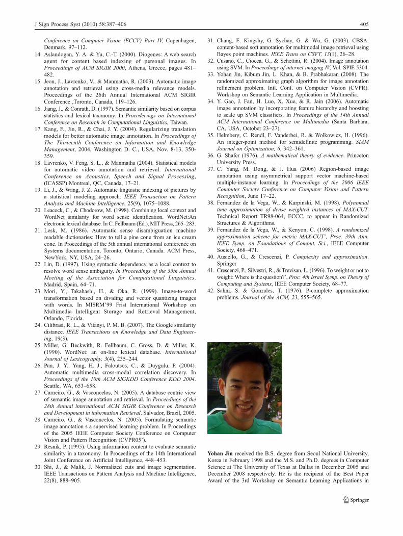
Yohan Jin received the B.S. degree from Seoul National University,Korea in February 1998 and the M.S. and Ph.D. degrees in ComputerScience at The University of Texas at Dallas in December 2005 andDecember 2008 respectively. He is the recipient of the Best PaperAward of the 3rd Workshop on Semantic Learning Applications in


Multimedia 2008 IEEE Conference on Computer Vision and PatternRecognition (CVPR). He is currently working at Data-Mining Teamof MySpace Inc. from September 2008.

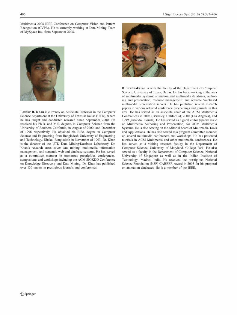
Latifur R. Khan is currently an Associate Professor in the ComputerScience department at the University of Texas at Dallas (UTD), wherehe has taught and conducted research since September 2000. Hereceived his Ph.D. and M.S. degrees in Computer Science from theUniversity of Southern California, in August of 2000, and Decemberof 1996 respectively. He obtained his B.Sc. degree in ComputerScience and Engineering from Bangladesh University of Engineeringand Technology, Dhaka, Bangladesh in November of 1993. Dr. Khanis the director of the UTD Data Mining/Database Laboratory. Dr.Khan’s research areas cover data mining, multimedia informationmanagement, and semantic web and database systems. He has servedas a committee member in numerous prestigious conferences,symposiums and workshops including the ACM SIGKDD Conferenceon Knowledge Discovery and Data Mining. Dr. Khan has publishedover 130 papers in prestigious journals and conferences.

B. Prabhakaran is with the faculty of the Department of ComputerScience, University of Texas, Dallas. He has been working in the areaof multimedia systems: animation and multimedia databases, author-ing and presentation, resource management, and scalable Webbasedmultimedia presentation servers. He has published several researchpapers in various refereed conference proceedings and journals in thisarea. He has served as an associate chair of the ACM MultimediaConferences in 2003 (Berkeley, California), 2000 (Los Angeles), and1999 (Orlando, Florida). He has served as a guest editor (special issueon Multimedia Authoring and Presentation) for ACM MultimediaSystems. He is also serving on the editorial board of Multimedia Toolsand Applications. He has also served as a program committee memberon several multimedia conferences and workshops. He has presentedtutorials in ACM Multimedia and other multimedia conferences. Hehas served as a visiting research faculty in the Department ofComputer Science, University of Maryland, College Park. He alsoserved as a faculty in the Department of Computer Science, NationalUniversity of Singapore as well as in the Indian Institute ofTechnology, Madras, India. He received the prestigious NationalScience Foundation (NSF) CAREER Award in 2003 for his proposalon animation databases. He is a member of the IEEE.


knowledge based image annotation refinementlkhan/papers/knowledge-based image annotation... ·...

Documents