knots, graphs and surfaces - math.csi.cuny.eduikofman/ribbon_graphs.pdf · knots, graphs and...
TRANSCRIPT
Knots, graphs and surfaces
Ilya Kofman
College of Staten Island and The Graduate CenterCity University of New York (CUNY)
May 30, 2012
Ilya Kofman (CUNY – CSI & GC) Knots, graphs and surfaces 1 / 33
Early knot theory
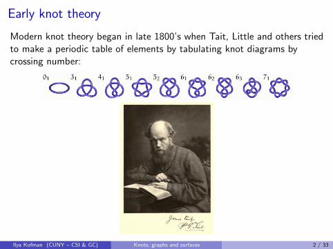
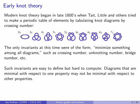
Modern knot theory began in late 1800’s when Tait, Little and others triedto make a periodic table of elements by tabulating knot diagrams bycrossing number:
The only invariants at this time were of the form, “minimize somethingamong all diagrams,” such as crossing number, unknotting number, bridgenumber, etc.
Such invariants are easy to define but hard to compute: Diagrams that areminimal with respect to one property may not be minimal with respect toother properties.
Ilya Kofman (CUNY – CSI & GC) Knots, graphs and surfaces 2 / 33
Early knot theory
Modern knot theory began in late 1800’s when Tait, Little and others triedto make a periodic table of elements by tabulating knot diagrams bycrossing number:
The only invariants at this time were of the form, “minimize somethingamong all diagrams,” such as crossing number, unknotting number, bridgenumber, etc.
Such invariants are easy to define but hard to compute: Diagrams that areminimal with respect to one property may not be minimal with respect toother properties.
Ilya Kofman (CUNY – CSI & GC) Knots, graphs and surfaces 2 / 33
Tait graph
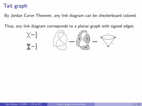
By Jordan Curve Theorem, any link diagram can be checkerboard colored.
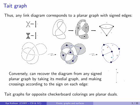
Thus, any link diagram corresponds to a planar graph with signed edges:
��������������������������������������������
��������������������������������������������
��������������������������������������������
��������������������������������������������
�������������������������������������������������������
�������������������������������������������������������
�������������������������������������������������������
�������������������������������������������������������
����������������������������������������������������������������������������������������
����������������������������������������������������������������������������������������
���������������
���������������
������������
������������
���������������������������������������������������������������������������������������������������
���������������������������������������������������������������������������������������������������
������������������������������
������������������������������������
������������������������
������������������������������
������������������������������������������������������������������������������������������������������������������������
������������������������������������������������������������������������������������������������������������������������
������������������������������������������������������������������������������������������������������������������������������������������������������������������������������������������������������������
������������������������������������������������������������������������������������������������������������������������������������������������������������������������������������������������������������
������������������������������������������������������������������������������������������������������������������������������������������������������������������������������������������������������������������������������������������������������������������������������������������������������������������������������������������������������������������������������������������������������������������������������
������������������������������������������������������������������������������������������������������������������������������������������������������������������������������������������������������������������������������������������������������������������������������������������������������������������������������������������������������������������������������������������������������������������������������
���������
���������
������������
������������
������������
������������
������������
Ilya Kofman (CUNY – CSI & GC) Knots, graphs and surfaces 3 / 33

Tait graph
By Jordan Curve Theorem, any link diagram can be checkerboard colored.
Thus, any link diagram corresponds to a planar graph with signed edges:
��������������������������������������������
��������������������������������������������
��������������������������������������������
��������������������������������������������
�������������������������������������������������������
�������������������������������������������������������
�������������������������������������������������������
�������������������������������������������������������
����������������������������������������������������������������������������������������
����������������������������������������������������������������������������������������
���������������
���������������
������������
������������
���������������������������������������������������������������������������������������������������
���������������������������������������������������������������������������������������������������
������������������������������
������������������������������������
������������������������
������������������������������
������������������������������������������������������������������������������������������������������������������������
������������������������������������������������������������������������������������������������������������������������
������������������������������������������������������������������������������������������������������������������������������������������������������������������������������������������������������������
������������������������������������������������������������������������������������������������������������������������������������������������������������������������������������������������������������
������������������������������������������������������������������������������������������������������������������������������������������������������������������������������������������������������������������������������������������������������������������������������������������������������������������������������������������������������������������������������������������������������������������������������
������������������������������������������������������������������������������������������������������������������������������������������������������������������������������������������������������������������������������������������������������������������������������������������������������������������������������������������������������������������������������������������������������������������������������
���������
���������
������������
������������
������������
������������
������������
Ilya Kofman (CUNY – CSI & GC) Knots, graphs and surfaces 3 / 33
Tait graph
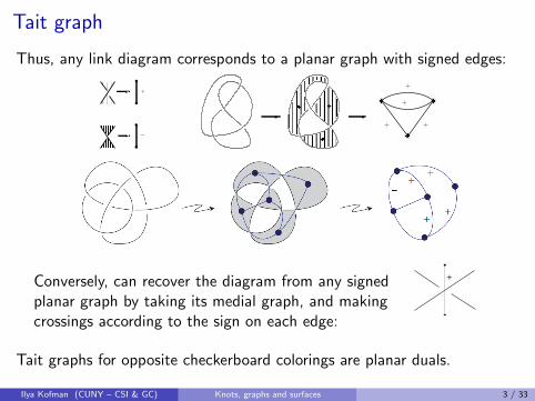
Thus, any link diagram corresponds to a planar graph with signed edges:
��������������������������������������������
��������������������������������������������
��������������������������������������������
��������������������������������������������
�������������������������������������������������������
�������������������������������������������������������
�������������������������������������������������������
�������������������������������������������������������
����������������������������������������������������������������������������������������
����������������������������������������������������������������������������������������
���������������
���������������
������������
������������
���������������������������������������������������������������������������������������������������
���������������������������������������������������������������������������������������������������
������������������������������
������������������������������������
������������������������
������������������������������
������������������������������������������������������������������������������������������������������������������������
������������������������������������������������������������������������������������������������������������������������
������������������������������������������������������������������������������������������������������������������������������������������������������������������������������������������������������������
������������������������������������������������������������������������������������������������������������������������������������������������������������������������������������������������������������
������������������������������������������������������������������������������������������������������������������������������������������������������������������������������������������������������������������������������������������������������������������������������������������������������������������������������������������������������������������������������������������������������������������������������
������������������������������������������������������������������������������������������������������������������������������������������������������������������������������������������������������������������������������������������������������������������������������������������������������������������������������������������������������������������������������������������������������������������������������
���������
���������
������������
������������
������������
������������
������������
Conversely, can recover the diagram from any signedplanar graph by taking its medial graph, and makingcrossings according to the sign on each edge:
Tait graphs for opposite checkerboard colorings are planar duals.
Ilya Kofman (CUNY – CSI & GC) Knots, graphs and surfaces 3 / 33
Tait graph
Thus, any link diagram corresponds to a planar graph with signed edges:
��������������������������������������������
��������������������������������������������
��������������������������������������������
��������������������������������������������
�������������������������������������������������������
�������������������������������������������������������
�������������������������������������������������������
�������������������������������������������������������
����������������������������������������������������������������������������������������
����������������������������������������������������������������������������������������
���������������
���������������
������������
������������
���������������������������������������������������������������������������������������������������
���������������������������������������������������������������������������������������������������
������������������������������
������������������������������������
������������������������
������������������������������
������������������������������������������������������������������������������������������������������������������������
������������������������������������������������������������������������������������������������������������������������
������������������������������������������������������������������������������������������������������������������������������������������������������������������������������������������������������������
������������������������������������������������������������������������������������������������������������������������������������������������������������������������������������������������������������
������������������������������������������������������������������������������������������������������������������������������������������������������������������������������������������������������������������������������������������������������������������������������������������������������������������������������������������������������������������������������������������������������������������������������
������������������������������������������������������������������������������������������������������������������������������������������������������������������������������������������������������������������������������������������������������������������������������������������������������������������������������������������������������������������������������������������������������������������������������
���������
���������
������������
������������
������������
������������
������������
Conversely, can recover the diagram from any signedplanar graph by taking its medial graph, and makingcrossings according to the sign on each edge:
Tait graphs for opposite checkerboard colorings are planar duals.
Ilya Kofman (CUNY – CSI & GC) Knots, graphs and surfaces 3 / 33
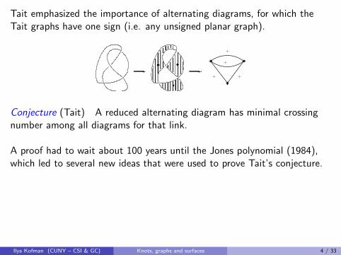
Tait emphasized the importance of alternating diagrams, for which theTait graphs have one sign (i.e. any unsigned planar graph).
������������������������������������������������������������������������������������������������������������������������
������������������������������������������������������������������������������������������������������������������������
������������������������������������������������������������������������������������������������������������������������������������������������������������������������������������������������������������
������������������������������������������������������������������������������������������������������������������������������������������������������������������������������������������������������������
������������������������������������������������������������������������������������������������������������������������������������������������������������������������������������������������������������������������������������������������������������������������������������������������������������������������������������������������������������������������������������������������������������������������������
������������������������������������������������������������������������������������������������������������������������������������������������������������������������������������������������������������������������������������������������������������������������������������������������������������������������������������������������������������������������������������������������������������������������������
���������
���������
������������
������������
������������
������������
������������
Conjecture (Tait) A reduced alternating diagram has minimal crossingnumber among all diagrams for that link.
A proof had to wait about 100 years until the Jones polynomial (1984),which led to several new ideas that were used to prove Tait’s conjecture.
Ilya Kofman (CUNY – CSI & GC) Knots, graphs and surfaces 4 / 33
Aside: Seifert surface
A turning point in knot theory was the discovery of the Alexanderpolynomial (1920’s), and its reinterpretation by Seifert (1930’s).
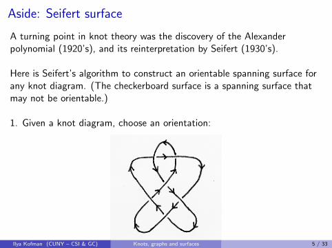
Here is Seifert’s algorithm to construct an orientable spanning surface forany knot diagram. (The checkerboard surface is a spanning surface thatmay not be orientable.)
1. Given a knot diagram, choose an orientation:
Ilya Kofman (CUNY – CSI & GC) Knots, graphs and surfaces 5 / 33

Aside: Seifert surface
A turning point in knot theory was the discovery of the Alexanderpolynomial (1920’s), and its reinterpretation by Seifert (1930’s).
Here is Seifert’s algorithm to construct an orientable spanning surface forany knot diagram. (The checkerboard surface is a spanning surface thatmay not be orientable.)
2. Splice the diagram according to the orientation:
Ilya Kofman (CUNY – CSI & GC) Knots, graphs and surfaces 5 / 33
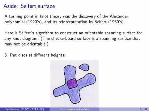
Aside: Seifert surface
A turning point in knot theory was the discovery of the Alexanderpolynomial (1920’s), and its reinterpretation by Seifert (1930’s).
Here is Seifert’s algorithm to construct an orientable spanning surface forany knot diagram. (The checkerboard surface is a spanning surface thatmay not be orientable.)
3. Put discs at different heights:
Ilya Kofman (CUNY – CSI & GC) Knots, graphs and surfaces 5 / 33
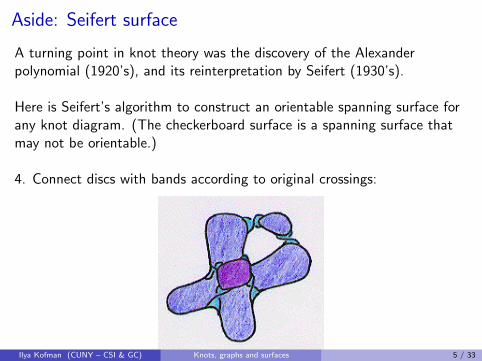
Aside: Seifert surface
A turning point in knot theory was the discovery of the Alexanderpolynomial (1920’s), and its reinterpretation by Seifert (1930’s).
Here is Seifert’s algorithm to construct an orientable spanning surface forany knot diagram. (The checkerboard surface is a spanning surface thatmay not be orientable.)
4. Connect discs with bands according to original crossings:
Ilya Kofman (CUNY – CSI & GC) Knots, graphs and surfaces 5 / 33
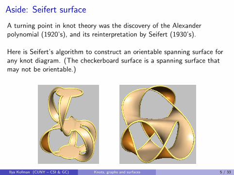
Aside: Seifert surface
A turning point in knot theory was the discovery of the Alexanderpolynomial (1920’s), and its reinterpretation by Seifert (1930’s).
Here is Seifert’s algorithm to construct an orientable spanning surface forany knot diagram. (The checkerboard surface is a spanning surface thatmay not be orientable.)
Ilya Kofman (CUNY – CSI & GC) Knots, graphs and surfaces 5 / 33
Aside: Seifert surface
The minimum genus of all Seifert surfaces for a given knot Kis called the genus of K , g(K ).
For any alternating diagram, Seifert’s algorithm produces the minimalgenus Seifert surface.
Unusual property: the genus of a knot can detect Conway mutation.
From the Seifert surface, can construct the Seifert matrix to get otherimportant invariants: determinant, signature, Alexander polynomial.
Ilya Kofman (CUNY – CSI & GC) Knots, graphs and surfaces 5 / 33
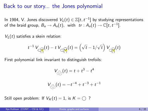
Back to our story... the Jones polynomial
In 1984, V. Jones discovered VL(t) ∈ Z[t, t−1] by studying representationsof the braid group, Bn → An(t), with tr : An(t)→ C[t, t−1].
VL(t) satisfies a skein relation:
t−1 V (t)− t V (t) =(√
t − 1/√
t)
V (t)
First polynomial link invariant to distinguish trefoils:
V (t) = t + t3 − t4
V (t) = −t−4 + t−3 + t−1
Still open problem: If VK (t) = 1, is K =© ?
Ilya Kofman (CUNY – CSI & GC) Knots, graphs and surfaces 6 / 33
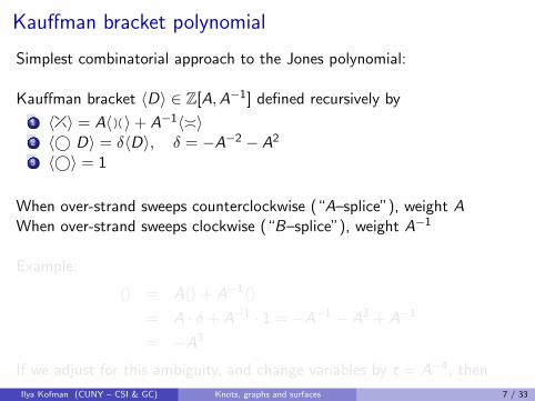
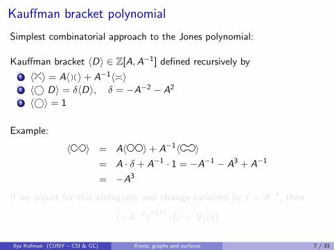
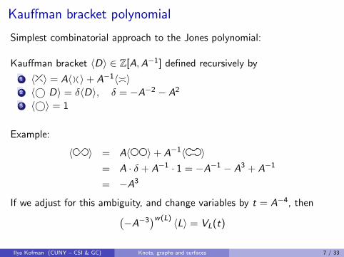
Kauffman bracket polynomial
Simplest combinatorial approach to the Jones polynomial:
Kauffman bracket 〈D〉 ∈ Z[A,A−1] defined recursively by
1 〈 〉 = A〈 � 〉+ A−1〈�〉2 〈© D〉 = δ〈D〉, δ = −A−2 − A2
3 〈©〉 = 1
When over-strand sweeps counterclockwise (“A–splice”), weight AWhen over-strand sweeps clockwise (“B–splice”), weight A−1
Example:
〈〉 = A〈〉+ A−1〈〉= A · δ + A−1 · 1 = −A−1 − A3 + A−1
= −A3
If we adjust for this ambiguity, and change variables by t = A−4, then(−A−3
)w(L) 〈L〉 = VL(t)Ilya Kofman (CUNY – CSI & GC) Knots, graphs and surfaces 7 / 33
Kauffman bracket polynomial
Simplest combinatorial approach to the Jones polynomial:
Kauffman bracket 〈D〉 ∈ Z[A,A−1] defined recursively by
1 〈 〉 = A〈 � 〉+ A−1〈�〉2 〈© D〉 = δ〈D〉, δ = −A−2 − A2
3 〈©〉 = 1
Example:
〈 〉 = A〈 〉+ A−1〈 〉= A · δ + A−1 · 1 = −A−1 − A3 + A−1
= −A3
If we adjust for this ambiguity, and change variables by t = A−4, then(−A−3
)w(L) 〈L〉 = VL(t)
Ilya Kofman (CUNY – CSI & GC) Knots, graphs and surfaces 7 / 33
Kauffman states
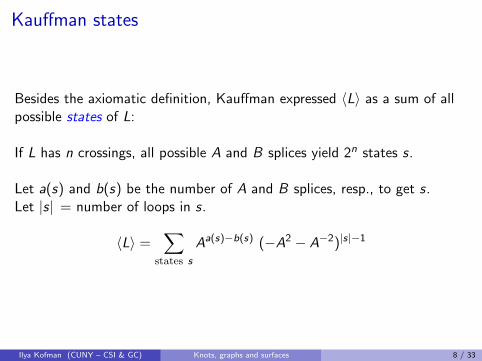
Besides the axiomatic definition, Kauffman expressed 〈L〉 as a sum of allpossible states of L:
If L has n crossings, all possible A and B splices yield 2n states s.
Let a(s) and b(s) be the number of A and B splices, resp., to get s.Let |s| = number of loops in s.
〈L〉 =∑
states s
Aa(s)−b(s) (−A2 − A−2)|s|−1
Ilya Kofman (CUNY – CSI & GC) Knots, graphs and surfaces 8 / 33
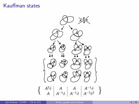
Kauffman states
{ A3δ A A A−1δA A−1δ A−1δ A−3δ2
}Ilya Kofman (CUNY – CSI & GC) Knots, graphs and surfaces 8 / 33
Turaev surface
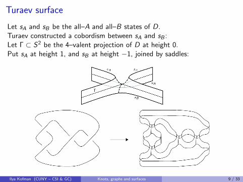
Let sA and sB be the all–A and all–B states of D.Turaev constructed a cobordism between sA and sB :Let Γ ⊂ S2 be the 4–valent projection of D at height 0.Put sA at height 1, and sB at height −1, joined by saddles:
Ilya Kofman (CUNY – CSI & GC) Knots, graphs and surfaces 9 / 33
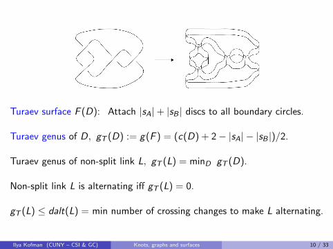
Turaev surface F (D): Attach |sA|+ |sB | discs to all boundary circles.
Turaev genus of D, gT (D) := g(F ) = (c(D) + 2− |sA| − |sB |)/2.
Turaev genus of non-split link L, gT (L) = minD gT (D).
Non-split link L is alternating iff gT (L) = 0.
gT (L) ≤ dalt(L) = min number of crossing changes to make L alternating.
Ilya Kofman (CUNY – CSI & GC) Knots, graphs and surfaces 10 / 33
Proof of Tait’s conjecture
Conjecture (Tait) A reduced alternating diagram D has minimal crossingnumber among all diagrams for the alternating link L.
The proof follows from two claims:
1. Although defined for diagrams, the Jones polynomial VL(t) is a linkinvariant.
2. sA and sB contribute the extreme terms ±tα and ±tβ of VL(t).
max degA〈D〉 −min degA〈D〉 ≤ 2(c(D) + sA(D) + sB(D)− 2)
with equality if D is alternating (generally, adequate).
So for any link `, span V`(t) = α− β ≤ c(`)− gT (`), with equality if ` isadequate. Thus,
span VL(t) = c(L) if L is alternating.
Ilya Kofman (CUNY – CSI & GC) Knots, graphs and surfaces 11 / 33
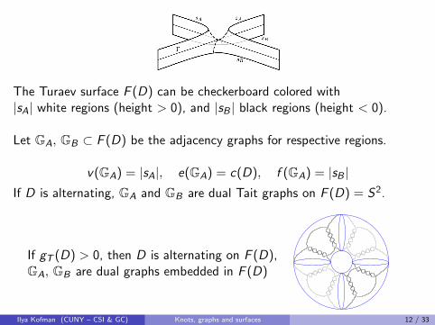
The Turaev surface F (D) can be checkerboard colored with|sA| white regions (height > 0), and |sB | black regions (height < 0).
Let GA, GB ⊂ F (D) be the adjacency graphs for respective regions.
v(GA) = |sA|, e(GA) = c(D), f (GA) = |sB |If D is alternating, GA and GB are dual Tait graphs on F (D) = S2.
If gT (D) > 0, then D is alternating on F (D),GA, GB are dual graphs embedded in F (D)
Ilya Kofman (CUNY – CSI & GC) Knots, graphs and surfaces 12 / 33
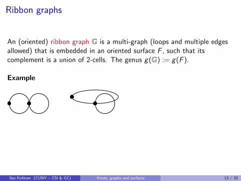
Ribbon graphs
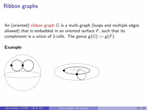
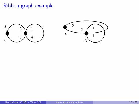
An (oriented) ribbon graph G is a multi-graph (loops and multiple edgesallowed) that is embedded in an oriented surface F , such that itscomplement is a union of 2-cells. The genus g(G) := g(F ).
Example
Ilya Kofman (CUNY – CSI & GC) Knots, graphs and surfaces 13 / 33
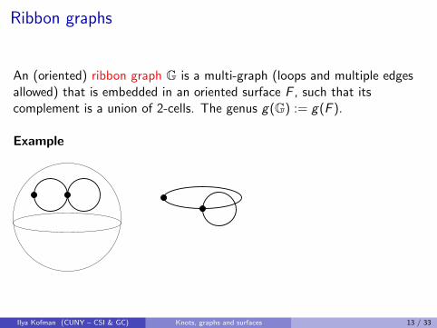
Ribbon graphs
An (oriented) ribbon graph G is a multi-graph (loops and multiple edgesallowed) that is embedded in an oriented surface F , such that itscomplement is a union of 2-cells. The genus g(G) := g(F ).
Example
Ilya Kofman (CUNY – CSI & GC) Knots, graphs and surfaces 13 / 33
Ribbon graphs
An (oriented) ribbon graph G is a multi-graph (loops and multiple edgesallowed) that is embedded in an oriented surface F , such that itscomplement is a union of 2-cells. The genus g(G) := g(F ).
Example
Ilya Kofman (CUNY – CSI & GC) Knots, graphs and surfaces 13 / 33
Algebraic definition
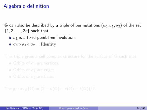
G can also be described by a triple of permutations (σ0, σ1, σ2) of the set{1, 2, . . . , 2n} such that
σ1 is a fixed-point-free involution.
σ0 ◦ σ1 ◦ σ2 = Identity
This triple gives a cell complex structure for the surface of G such that
Orbits of σ0 are vertices.
Orbits of σ1 are edges.
Orbits of σ2 are faces.
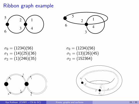
The genus g(G) = (2− v(G) + e(G)− f (G))/2.
Ilya Kofman (CUNY – CSI & GC) Knots, graphs and surfaces 14 / 33
Algebraic definition
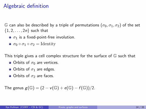
G can also be described by a triple of permutations (σ0, σ1, σ2) of the set{1, 2, . . . , 2n} such that
σ1 is a fixed-point-free involution.
σ0 ◦ σ1 ◦ σ2 = Identity
This triple gives a cell complex structure for the surface of G such that
Orbits of σ0 are vertices.
Orbits of σ1 are edges.
Orbits of σ2 are faces.
The genus g(G) = (2− v(G) + e(G)− f (G))/2.
Ilya Kofman (CUNY – CSI & GC) Knots, graphs and surfaces 14 / 33
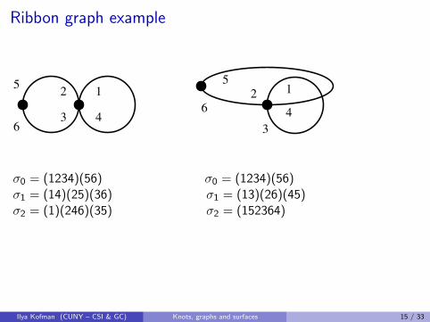
Ribbon graph example
Ilya Kofman (CUNY – CSI & GC) Knots, graphs and surfaces 15 / 33
Ribbon graph example
43
125
6
6
1
3
4
2
5
Ilya Kofman (CUNY – CSI & GC) Knots, graphs and surfaces 15 / 33
Ribbon graph example
43
125
6
6
1
3
4
2
5
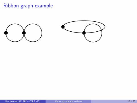
σ0 = (1234)(56) σ0 = (1234)(56)σ1 = (14)(25)(36) σ1 = (13)(26)(45)σ2 = (1)(246)(35) σ2 = (152364)
Ilya Kofman (CUNY – CSI & GC) Knots, graphs and surfaces 15 / 33
Ribbon graph example
43
125
6
6
1
3
4
2
5
σ0 = (1234)(56) σ0 = (1234)(56)σ1 = (14)(25)(36) σ1 = (13)(26)(45)σ2 = (1)(246)(35) σ2 = (152364)
Ilya Kofman (CUNY – CSI & GC) Knots, graphs and surfaces 15 / 33
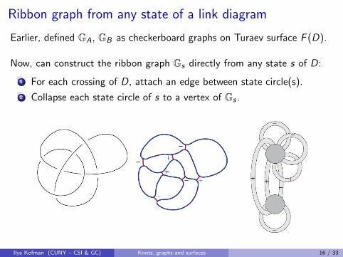
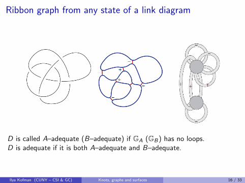
Ribbon graph from any state of a link diagram
Earlier, defined GA, GB as checkerboard graphs on Turaev surface F (D).
Now, can construct the ribbon graph Gs directly from any state s of D:
1 For each crossing of D, attach an edge between state circle(s).
2 Collapse each state circle of s to a vertex of Gs .
Ilya Kofman (CUNY – CSI & GC) Knots, graphs and surfaces 16 / 33
Ribbon graph from any state of a link diagram
D is called A–adequate (B–adequate) if GA (GB) has no loops.D is adequate if it is both A–adequate and B–adequate.
Ilya Kofman (CUNY – CSI & GC) Knots, graphs and surfaces 16 / 33
Applications to geometry and topology of S3 − K
We highlight some recent results by Futer, Kalfagianni, Purcell.
Main idea: Relate certain stable coefficients of colored Jones polynomialsto fibering data and hyperbolic volume bounds using incompressible statesurfaces.
Gs ⊂ Fs , state surface constructed like Seifert surface; Gs is spine for Fs .Fs is orientable (i.e. a Seifert surface) iff Gs is bipartite.
Thm. (Ozawa) FA is incompressible and ∂–incompressible in S3 − L iff Lis A–adequate. Similarly for FB .
Ilya Kofman (CUNY – CSI & GC) Knots, graphs and surfaces 17 / 33
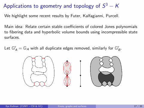
Applications to geometry and topology of S3 − K
We highlight some recent results by Futer, Kalfagianni, Purcell.
Main idea: Relate certain stable coefficients of colored Jones polynomialsto fibering data and hyperbolic volume bounds using incompressible statesurfaces.
Let G′A = GA with all duplicate edges removed, similarly for G′B .
Ilya Kofman (CUNY – CSI & GC) Knots, graphs and surfaces 17 / 33
Applications to geometry and topology of S3 − K
We highlight some recent results by Futer, Kalfagianni, Purcell.
Main idea: Relate certain stable coefficients of colored Jones polynomialsto fibering data and hyperbolic volume bounds using incompressible statesurfaces.
Thm. If D is an A–adequate diagram of a hyperbolic link K ,
vol(S3 − K ) ≥ v8(χ−(G′A)− E (D))
Thm. S3 − K fibers over S1 with fiber FA iff G′A is a tree.
If K is A–adequate, let βK = penultimate coefficient of JnK (t), which
stabilizes for n > 1.
Cor. S3 − K fibers over S1 with fiber FA iff βK = 0.
Ilya Kofman (CUNY – CSI & GC) Knots, graphs and surfaces 17 / 33
Related polynomial invariants
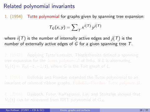
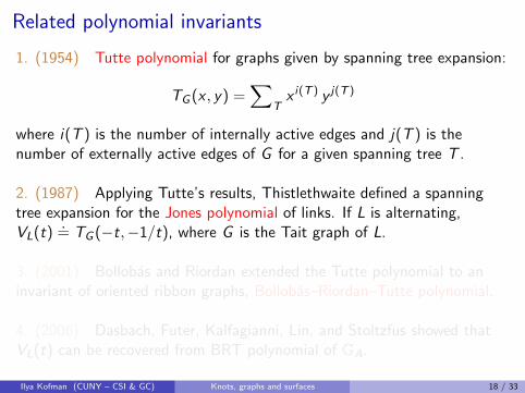
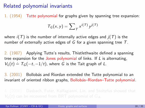
1. (1954) Tutte polynomial for graphs given by spanning tree expansion:
TG (x , y) =∑
Tx i(T ) y j(T )
where i(T ) is the number of internally active edges and j(T ) is thenumber of externally active edges of G for a given spanning tree T .
2. (1987) Applying Tutte’s results, Thistlethwaite defined a spanningtree expansion for the Jones polynomial of links. If L is alternating,VL(t)
.= TG (−t,−1/t), where G is the Tait graph of L.
3. (2001) Bollobas and Riordan extended the Tutte polynomial to aninvariant of oriented ribbon graphs, Bollobas–Riordan–Tutte polynomial.
4. (2006) Dasbach, Futer, Kalfagianni, Lin, and Stoltzfus showed thatVL(t) can be recovered from BRT polynomial of GA.
Ilya Kofman (CUNY – CSI & GC) Knots, graphs and surfaces 18 / 33
Related polynomial invariants
1. (1954) Tutte polynomial for graphs given by spanning tree expansion:
TG (x , y) =∑
Tx i(T ) y j(T )
where i(T ) is the number of internally active edges and j(T ) is thenumber of externally active edges of G for a given spanning tree T .
2. (1987) Applying Tutte’s results, Thistlethwaite defined a spanningtree expansion for the Jones polynomial of links. If L is alternating,VL(t)
.= TG (−t,−1/t), where G is the Tait graph of L.
3. (2001) Bollobas and Riordan extended the Tutte polynomial to aninvariant of oriented ribbon graphs, Bollobas–Riordan–Tutte polynomial.
4. (2006) Dasbach, Futer, Kalfagianni, Lin, and Stoltzfus showed thatVL(t) can be recovered from BRT polynomial of GA.
Ilya Kofman (CUNY – CSI & GC) Knots, graphs and surfaces 18 / 33
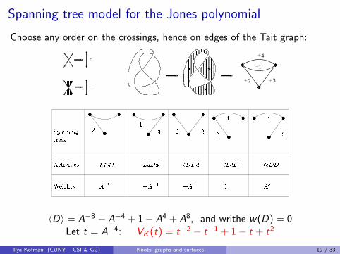
Spanning tree model for the Jones polynomial
Choose any order on the crossings, hence on edges of the Tait graph:
��������������������������������������������
��������������������������������������������
��������������������������������������������
��������������������������������������������
�������������������������������������������������������
�������������������������������������������������������
�������������������������������������������������������
�������������������������������������������������������
����������������������������������������������������������������������������������������
����������������������������������������������������������������������������������������
���������������
���������������
������������
������������
���������������������������������������������������������������������������������������������������
���������������������������������������������������������������������������������������������������
������������������������������
������������������������������������
������������������������
������������������������������
������������������������������������������������������������������������������������������������������������������������
������������������������������������������������������������������������������������������������������������������������
������������������������������������������������������������������������������������������������������������������������������������������������������������������������������������������������������������
������������������������������������������������������������������������������������������������������������������������������������������������������������������������������������������������������������
������������������������������������������������������������������������������������������������������������������������������������������������������������������������������������������������������������������������������������������������������������������������������������������������������������������������������������������������������������������������������������������������������������������������������
������������������������������������������������������������������������������������������������������������������������������������������������������������������������������������������������������������������������������������������������������������������������������������������������������������������������������������������������������������������������������������������������������������������������������
32
4
1���������
���������
������������
������������
������������
������������
������������
〈D〉 = A−8 − A−4 + 1− A4 + A8, and writhe w(D) = 0Let t = A−4: VK (t) = t−2 − t−1 + 1− t + t2
Ilya Kofman (CUNY – CSI & GC) Knots, graphs and surfaces 19 / 33
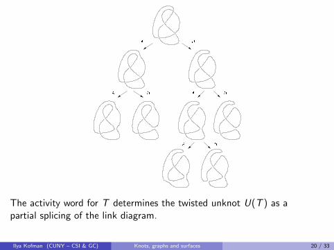
The activity word for T determines the twisted unknot U(T ) as apartial splicing of the link diagram.
Ilya Kofman (CUNY – CSI & GC) Knots, graphs and surfaces 20 / 33
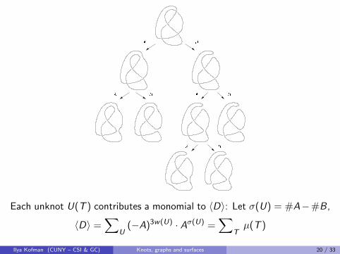
Each unknot U(T ) contributes a monomial to 〈D〉: Let σ(U) = #A−#B,
〈D〉 =∑
U(−A)3w(U) · Aσ(U) =
∑Tµ(T )
Ilya Kofman (CUNY – CSI & GC) Knots, graphs and surfaces 20 / 33
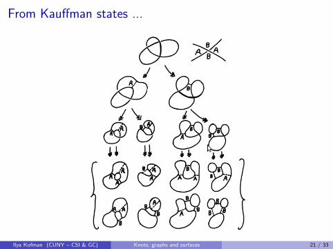
From Kauffman states ...
Ilya Kofman (CUNY – CSI & GC) Knots, graphs and surfaces 21 / 33
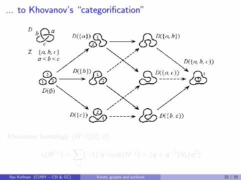
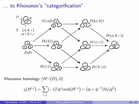
... to Khovanov’s “categorification”
Khovanov homology {H i , j(D), ∂}
χ(H i , j) =∑i , j
(−1)iq jrank(H i , j) = (q + q−1)VL(q2)
Ilya Kofman (CUNY – CSI & GC) Knots, graphs and surfaces 22 / 33
... to Khovanov’s “categorification”
Khovanov homology {H i , j(D), ∂}
χ(H i , j) =∑i , j
(−1)iq jrank(H i , j) = (q + q−1)VL(q2)
Ilya Kofman (CUNY – CSI & GC) Knots, graphs and surfaces 22 / 33
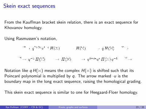
Skein exact sequences
From the Kauffman bracket skein relation, there is an exact sequence forKhovanov homology.
Using Rasmussen’s notation,
Notation like q H(�) means the complex H(�) is shifted such that itsPoincare polynomial is multiplied by q. The arrow marked ·u is theboundary map in the long exact sequence, raising the homological grading.
This skein exact sequence is similar to one for Heegaard-Floer homology.
Ilya Kofman (CUNY – CSI & GC) Knots, graphs and surfaces 23 / 33
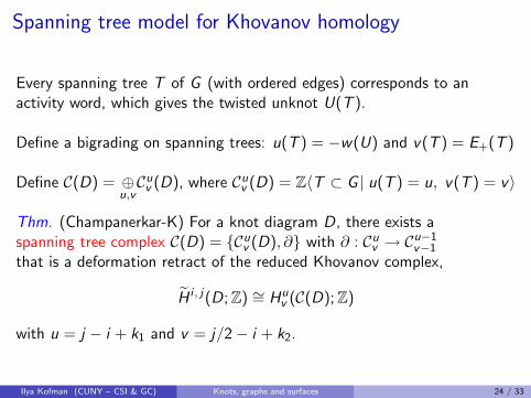
Spanning tree model for Khovanov homology
Every spanning tree T of G (with ordered edges) corresponds to anactivity word, which gives the twisted unknot U(T ).
Define a bigrading on spanning trees: u(T ) = −w(U) and v(T ) = E+(T )
Define C(D) = ⊕u,vCu
v (D), where Cuv (D) = Z〈T ⊂ G | u(T ) = u, v(T ) = v〉
Thm. (Champanerkar-K) For a knot diagram D, there exists aspanning tree complex C(D) = {Cu
v (D), ∂} with ∂ : Cuv → Cu−1
v−1
that is a deformation retract of the reduced Khovanov complex,
H i , j(D; Z) ∼= Huv (C(D); Z)
with u = j − i + k1 and v = j/2− i + k2.
Ilya Kofman (CUNY – CSI & GC) Knots, graphs and surfaces 24 / 33
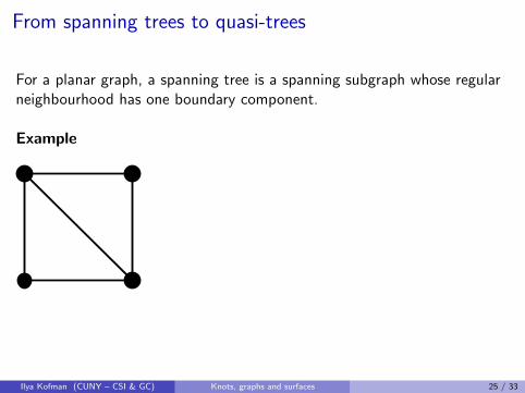
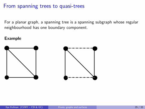
From spanning trees to quasi-trees
For a planar graph, a spanning tree is a spanning subgraph whose regularneighbourhood has one boundary component.
Example
Ilya Kofman (CUNY – CSI & GC) Knots, graphs and surfaces 25 / 33
From spanning trees to quasi-trees
For a planar graph, a spanning tree is a spanning subgraph whose regularneighbourhood has one boundary component.
Example
Ilya Kofman (CUNY – CSI & GC) Knots, graphs and surfaces 25 / 33
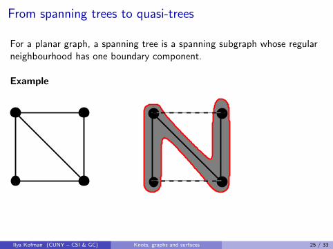
From spanning trees to quasi-trees
For a planar graph, a spanning tree is a spanning subgraph whose regularneighbourhood has one boundary component.
Example
Ilya Kofman (CUNY – CSI & GC) Knots, graphs and surfaces 25 / 33
Quasi-trees
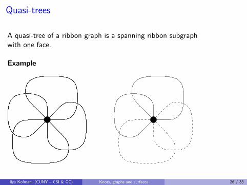
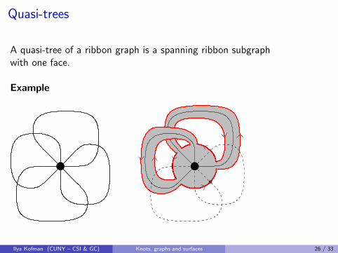
A quasi-tree of a ribbon graph is a spanning ribbon subgraphwith one face.
Example
Ilya Kofman (CUNY – CSI & GC) Knots, graphs and surfaces 26 / 33
Quasi-trees
A quasi-tree of a ribbon graph is a spanning ribbon subgraphwith one face.
Example
Ilya Kofman (CUNY – CSI & GC) Knots, graphs and surfaces 26 / 33
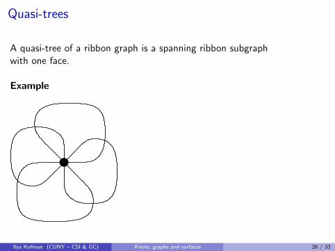
Quasi-trees
A quasi-tree of a ribbon graph is a spanning ribbon subgraphwith one face.
Example
Ilya Kofman (CUNY – CSI & GC) Knots, graphs and surfaces 26 / 33
Quasi-trees
A quasi-tree of a ribbon graph is a spanning ribbon subgraphwith one face.
Example
Ilya Kofman (CUNY – CSI & GC) Knots, graphs and surfaces 26 / 33
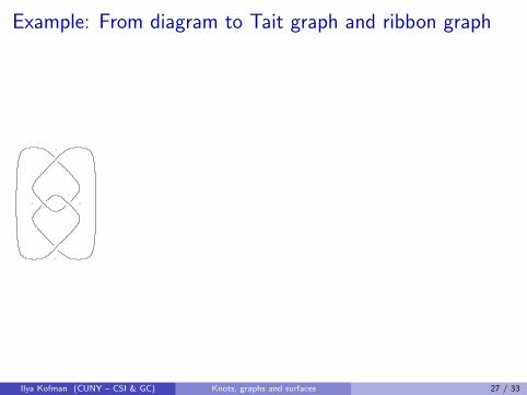
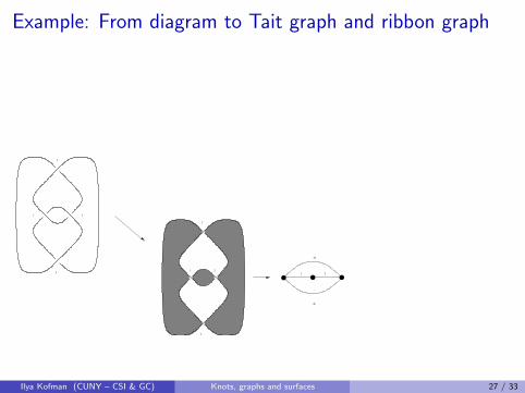
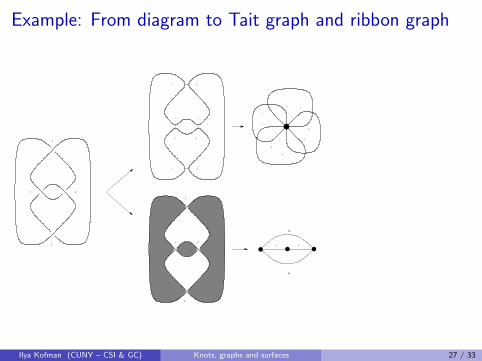
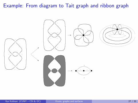
Example: From diagram to Tait graph and ribbon graph
3b
21
4b
1
1 2
3
4
3
4
3
8
1 2
1
6
7
2
3
8
4
2 4
5
7
65
6 8
5 7
1 2
3 4
Ilya Kofman (CUNY – CSI & GC) Knots, graphs and surfaces 27 / 33
Example: From diagram to Tait graph and ribbon graph
3b
21
4b
1
1 2
3
4
3
4
3
8
1 2
1
6
7
2
3
8
4
2 4
5
7
65
6 8
5 7
1 2
3 4
Ilya Kofman (CUNY – CSI & GC) Knots, graphs and surfaces 27 / 33
Example: From diagram to Tait graph and ribbon graph
3b
21
4b
1
1 2
3
4
3
4
3
8
1 2
1
6
7
2
3
8
4
2 4
5
7
65
6 8
5 7
1 2
3 4
Ilya Kofman (CUNY – CSI & GC) Knots, graphs and surfaces 27 / 33
Example: From diagram to Tait graph and ribbon graph
3b
21
4b
1
1 2
3
4
3
4
3
8
1 2
1
6
7
2
3
8
4
2 4
5
7
65
6 8
5 7
1 2
3 4
Ilya Kofman (CUNY – CSI & GC) Knots, graphs and surfaces 27 / 33
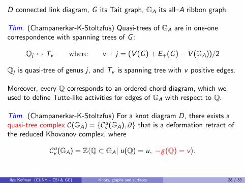
D connected link diagram, G its Tait graph, GA its all–A ribbon graph.
Thm. (Champanerkar-K-Stoltzfus) Quasi-trees of GA are in one-onecorrespondence with spanning trees of G :
Qj ↔ Tv where v + j = (V (G ) + E+(G )− V (GA))/2
Qj is quasi-tree of genus j , and Tv is spanning tree with v positive edges.
Moreover, every Q corresponds to an ordered chord diagram, which weused to define Tutte-like activities for edges of GA with respect to Q.
Thm. (Champanerkar-K-Stoltzfus) For a knot diagram D, there exists aquasi-tree complex C(GA) = {Cu
v (GA), ∂} that is a deformation retract ofthe reduced Khovanov complex, where
Cuv (GA) = Z〈Q ⊂ GA| u(Q) = u, −g(Q) = v〉.
Ilya Kofman (CUNY – CSI & GC) Knots, graphs and surfaces 28 / 33
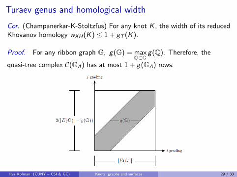
Turaev genus and homological width
Cor. (Champanerkar-K-Stoltzfus) For any knot K , the width of its reducedKhovanov homology wKH(K ) ≤ 1 + gT (K ).
Proof. For any ribbon graph G, g(G) = maxQ⊂G
g(Q). Therefore, the
quasi-tree complex C(GA) has at most 1 + g(GA) rows.
Ilya Kofman (CUNY – CSI & GC) Knots, graphs and surfaces 29 / 33
Turaev genus and homological width
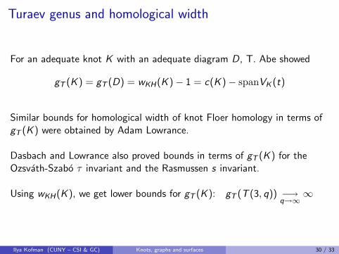
For an adequate knot K with an adequate diagram D, T. Abe showed
gT (K ) = gT (D) = wKH(K )− 1 = c(K )− spanVK (t)
Similar bounds for homological width of knot Floer homology in terms ofgT (K ) were obtained by Adam Lowrance.
Dasbach and Lowrance also proved bounds in terms of gT (K ) for theOzsvath-Szabo τ invariant and the Rasmussen s invariant.
Using wKH(K ), we get lower bounds for gT (K ): gT (T (3, q)) −→q→∞
∞
Ilya Kofman (CUNY – CSI & GC) Knots, graphs and surfaces 30 / 33
Turaev genus and homological width
For an adequate knot K with an adequate diagram D, T. Abe showed
gT (K ) = gT (D) = wKH(K )− 1 = c(K )− spanVK (t)
Similar bounds for homological width of knot Floer homology in terms ofgT (K ) were obtained by Adam Lowrance.
Dasbach and Lowrance also proved bounds in terms of gT (K ) for theOzsvath-Szabo τ invariant and the Rasmussen s invariant.
Using wKH(K ), we get lower bounds for gT (K ): gT (T (3, q)) −→q→∞
∞
Ilya Kofman (CUNY – CSI & GC) Knots, graphs and surfaces 30 / 33

Related open problems
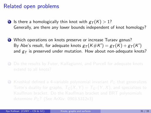
1 Is there a homologically thin knot with gT (K ) > 1?Generally, are there any lower bounds independent of knot homology?
2 Which operations on knots preserve or increase Turaev genus?By Abe’s result, for adequate knots gT (K#K ′) = gT (K ) + gT (K ′)and gT is preserved under mutation. How about non-adequate knots?
3 Do the results by Futer, Kalfagianni, and Purcell for adequate knotsextend to all knots?
4 Krushkal defined a 4-variable polynomial invariant PG that generalizesTutte’s duality for graphs, TG (X ,Y ) = TG∗(Y ,X ), and specializes toKauffman bracket. Do the Kauffman bracket and BRT polynomialsdetermine PG? (See ArXiv: 0903.5312v3)
Ilya Kofman (CUNY – CSI & GC) Knots, graphs and surfaces 31 / 33
Related open problems
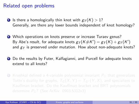
1 Is there a homologically thin knot with gT (K ) > 1?Generally, are there any lower bounds independent of knot homology?
2 Which operations on knots preserve or increase Turaev genus?By Abe’s result, for adequate knots gT (K#K ′) = gT (K ) + gT (K ′)and gT is preserved under mutation. How about non-adequate knots?
3 Do the results by Futer, Kalfagianni, and Purcell for adequate knotsextend to all knots?
4 Krushkal defined a 4-variable polynomial invariant PG that generalizesTutte’s duality for graphs, TG (X ,Y ) = TG∗(Y ,X ), and specializes toKauffman bracket. Do the Kauffman bracket and BRT polynomialsdetermine PG? (See ArXiv: 0903.5312v3)
Ilya Kofman (CUNY – CSI & GC) Knots, graphs and surfaces 31 / 33
Related open problems
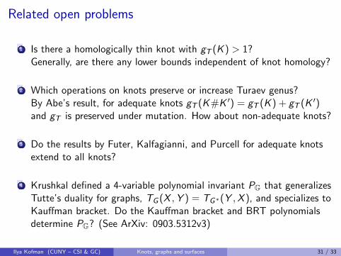
1 Is there a homologically thin knot with gT (K ) > 1?Generally, are there any lower bounds independent of knot homology?
2 Which operations on knots preserve or increase Turaev genus?By Abe’s result, for adequate knots gT (K#K ′) = gT (K ) + gT (K ′)and gT is preserved under mutation. How about non-adequate knots?
3 Do the results by Futer, Kalfagianni, and Purcell for adequate knotsextend to all knots?
4 Krushkal defined a 4-variable polynomial invariant PG that generalizesTutte’s duality for graphs, TG (X ,Y ) = TG∗(Y ,X ), and specializes toKauffman bracket. Do the Kauffman bracket and BRT polynomialsdetermine PG? (See ArXiv: 0903.5312v3)
Ilya Kofman (CUNY – CSI & GC) Knots, graphs and surfaces 31 / 33
Further reading from recent accessible papers
1 Jones polynomials, volume and essential knot surfaces: Asurvey by Futer, Kalfagianni, and Purcell. ArXiv: 1110.6388 (2011).
2 Partials duals of plane graphs, separability and the graphs ofknots by Moffatt. AGT 12 (2012) 1099-1136. ArXiv: 1007.4219(2012).
3 A Turaev surface approach to Khovanov homology by Dasbachand Lowrance. ArXiv: 1107.2344 (2011).
Thank you!
Ilya Kofman (CUNY – CSI & GC) Knots, graphs and surfaces 32 / 33
Image credits
p.2 Dror Bar-Natan, Wikipedia entry for Peter Guthrie Taitp.3 (second figure) Moffatt article abovep.5 (Seifert algorithm) Sharon Goldwaterp.5 (last two images) Produced with SeifertView by Jarke J. van Wijkp.8 Louis Kauffman Knots and Physicsp.9 (first figure) FKP article above, (second figure) Tetsuya Abep.16 Moffatt article abovep.17 FKP article abovep.22 Dror Bar-Natanp.29 Dasbach-Lowrance article above
(Almost) all other figures by Abhijit Champanerkar
Ilya Kofman (CUNY – CSI & GC) Knots, graphs and surfaces 33 / 33