keyhole effect in mimo wireless channels: measurements and theory

3596 IEEE TRANSACTIONS ON WIRELESS COMMUNICATIONS, VOL. 5, NO. 12, DECEMBER 2006

Keyhole Effect in MIMO Wireless Channels:Measurements and Theory

Peter Almers, Student Member, IEEE, Fredrik Tufvesson, Member, IEEE, and Andreas F. Molisch, Fellow, IEEE

Abstract— It has been predicted theoretically that for someenvironments, the capacity of wireless multiple-input multiple-output systems can become very low even for uncorrelatedsignals; this effect has been termed ”keyhole” or ”pinhole”.In this paper the first unique measurements of this effect arepresented. The measurements were performed in a controlledindoor environment that was designed to obtain a keyhole chan-nel. We analyze limitations due to measurement imperfectionsfor measurement-based capacity calculations and keyhole inves-tigations. We further present a bound for the higher eigenmodesas a function of the finite measurement signal-to-noise ratio andmultipath component leakage. The bound is compared to themeasurement results and shows excellent agreement. Finally, weanalyze the envelope distribution and, as expected from theory,it follows a double-Rayleigh distribution.

Index Terms— Keyhole, pinhole, MIMO, measurements, eigen-value, double-Rayleigh, capacity.

I. INTRODUCTION

MULTIPLE-INPUT multiple-output (MIMO) wirelesscommunication systems have multi-element antenna

arrays at both the transmitter and the receiver side. It hasbeen shown that they have the potential for large information-theoretic capacities, since the system can provide severalindependent communication channels between transmitter andreceiver [1], [2]. In an ideal multipath channel, the MIMOcapacity is approximately N times the capacity of a single-antenna system, where N is the smaller of the number oftransmit and receive antenna elements. Correlated signals atthe antenna elements lead to a decrease in the capacity - thiseffect has been investigated both theoretically [3], [4], andexperimentally [5]. It has recently been predicted theoreticallythat for some propagation scenarios, the MIMO channel ca-pacity can be low (i.e., comparable to the single-input single-output (SISO) capacity) even though the signals at the antennaelements are uncorrelated [6], [7], [8], [9], [10]. This effecthas been termed “keyhole” or “pinhole.”

The keyhole effect is related to scenarios where rich scatter-ing around the transmitter and receiver leads to low correlationof the signals, while other propagation effects, like diffraction

Manuscript received February 1, 2005; revised May 3, 2005; acceptedOctober 3, 2005. The associate editor coordinating the review of this paperand approving it for publication was M. Shafi. Parts of this material has beenpresented at IEEE GlobeCom 2004, San Francisco, USA.

P. Almers is with the Dept. of Electroscience, Lund University, Box 118,SE-221 00 Lund, Sweden (email: [email protected]).

F. Tufvesson is with the Dept. of Electroscience, Lund University, Box 118,SE-221 00 Lund, Sweden (email: [email protected]).

A. F. Molisch is with Mitsubishi Electric Research Labs, Cambridge, MA,USA, and also at the Department of Electroscience, Lund University, Box118, SE-22100 Lund, Sweden (email: [email protected]).

Digital Object Identifier 10.1109/TWC.2006.05025.

or waveguiding, lead to a rank reduction of the transfer func-tion matrix. Several previous measurement campaigns havesearched for the keyhole effect due to corridors, tunnels, ordiffraction in real environments [11]. While some indicationsfor rank reduction have been found, to our knowledge, nounambiguous measurements of a keyhole have been presentedin the literature.

In this paper, we present:

• Results of a measurement campaign that for the first timeunambiguously shows the keyhole effect experimentally.This includes the measured eigenvalue distribution.

• Separation of correlation and keyhole effects on outagecapacity.

• A confirmation by measurements of the theory for theenvelope statistics of a keyhole channel.

• An analysis of the impact of measurement noise onkeyhole channels.

• An upper bound for the eigenvalue for measured keyholechannels, as a function of the measurement signal-to-noise ratio (SNR).

In [12] we presented measurement results for a 6 × 6keyhole (rank-1) channel. In this paper we present extendedmeasurements (including both rank-1 and rank-3 channels)and an extensive analysis including bounds for the capacityof low rank systems. For reference and completeness we alsoinclude some results from the letter [12]. The measurementswere performed in a controlled indoor environment, wherethe propagation from one room to the next could only occurthrough a waveguide or a hole in the wall. The measurementresults show almost ideal keyhole properties; the capacity islow, the rank of the transfer matrix is nearly one though thecorrelation between the antenna elements is low.

The rest of the paper is organized as follows: after somebackground information on general MIMO channels (Sec. II)and low-rank MIMO channels (Sec. III), we describe thesetup of our experiment, describing both environment andmeasurement equipment in Sec. IV. As noise can never beperfectly excluded in an experiment, Sec. V gives an analysisof its impact on the measured eigenvalue distributions. Sec. VIthen derives upper bounds on the higher-order eigenvalues ofthe transfer function depending on the SNR. Sec. VII finallyprovides the measurement results, providing data for boththe eigenvalue distribution, the information-theoretic capacityresulting from it, and the amplitude distribution. A summaryconcludes the paper.

1536-1276/06$20.00 c© 2006 IEEE

ALMERS et al.: KEYHOLE EFFECT IN MIMO WIRELESS CHANNELS: MEASUREMENTS AND THEORY 3597

II. MIMO CHANNELS

In this paper we assume a single-user MIMO system withNT transmit and NR receive antenna elements, and flat fading.We use the conventional MIMO model and the received signalvector, y of size NR × 1 is written as

y = Hx + n, (1)

where H is the channel transfer matrix between the transmitterand the receiver of size NR × NT normalized as,

E[‖H‖2

F

]= NRNT. (2)

Further, x is the transmitted signal vector, andn ∈CN (

0, σ2nI[NR×1]

)represents noise, where I[NR×1]

is the identity vector.For equal power allocation between the transmitter elements

(no waterfilling), the instantaneous channel capacity [bit/s/Hz]for the channel model in (1) can be calculated as [2]

C = log2

(det(I +

γeval

NTWH

)), (3)

or expressed in singular values

C =K∑

k=1

log2

(1 +

γeval

NT|sk (H)|2

), (4)

where

WH={

HH†

H†Hfor NR ≤ NT

for NT < NR, (5)

[·]† denotes the complex conjugate transpose, and sk (H), isthe k :th singular value of H. Further, γeval is the evaluationSNR, i.e., the signal-to-noise ratio (SNR) that the capacity isevaluated for, defined as

γeval =E[h (k, l)h† (k, l)

]E [n (k)n† (k)]

=σ2

h

σ2n

=1σ2

n

, (6)

where E [·] is the expectation1, h (k, l) and n (k) are the k, l :thentry in H and k :th entry in n, respectively, σ2

h is the powerof the complex entries in H, and normalized to one from (2).It is assumed that x has unit energy.

When measuring a MIMO transfer matrix, the measuredquantity will consist of contributions not only from multi-path components (MPCs) but also from measurement noise.The measured keyhole transfer matrix can be modelled as

Hmeas= Hkey+Nmeas, (7)

where Nmeas∈CN(0, σ2

nmeasI)

denotes the measurement noisematrix. The measurement SNR, γmeas, can then be defined as

γmeas =E[hkey (k, l)h†

key (k, l)]

E[nmeas (k, l)n†

meas (k, l)] =

σ2hkey

σ2nmeas

. (8)

1For a deterministic channel, the expectation is taken over the noiserealizations only. For a randomly varying channel (as will be considered inthe remainder of the paper), the expectation is taken also over the channelrealizations.

III. LOW RANK MIMO CHANNELS

The channel capacity is highly dependent on the distributionof the singular values of the normalized channel transfermatrix H, see Eq. 4. The two extreme cases for the singularvalue distributions of H, in a capacity sense, are:

• equally strong singular values → maximum MIMO ca-pacity, which is min (NR, NT) times higher than for theSISO channel.

• only one non-zero singular value → minimum MIMOcapacity, with only the receiver array gain affecting thecapacity.

A skew singular value distribution occurs when the correla-tions of the signals at the receiver and/or transmitter antennaelements are high. However, a skew singular value distributioncan also occur with a low correlation between the antennaelements due to the rank of the propagation channel. Withzero correlation and only one non-zero singular value it istermed keyhole or pinhole channel [6], [7], [8], [9].

A. Correlated channels

It is well known that correlation between the antennaelements at the transmitter and/or the receiver reduces thecapacity [3], [4], [13], hence the (complex) spatial correlationis an important parameter in describing MIMO channels. Ahigh correlation between receiver and/or transmitter elementscould be a result of mutual coupling between elements and/ordue to propagation channel effects such as low angular spread,strong line-of-sight (LOS), or a small number of MPCs. In thissection we define the most common correlations measures.

The full correlation, R, between all possible combinationsof the entries in the channel matrix, H, is defined as

R = E[vec (H) · vec (H)†

], (9)

where the operator vec(·) stacks the columns in the matrix ina column vector. If the receive correlation is the same for alltransmitted MPCs, R can be decomposed as [14], [15]

R = RT⊗RR, (10)

where ⊗ is the Kronecker product. The marginal correlationmatrices are

RR =1

NTE[HH†

], (11)

and

RT =1

NRE[H†H

]T, (12)

where [·]T is the matrix transpose. RR and RT describe thecorrelation between the signals at receiver and transmitterelements, respectively. The Kronecker model’s tractability forMIMO channel theoretical investigations has made it morewidespread than the full correlation model. According tothe Kronecker model, the channel, and thus the capacity, iscompletely determined by the correlations at transmitter andreceiver side. In order to compare the capacity reduction dueto receive and transmit correlation to the capacity reductiondue to the keyhole effect, we use the Kronecker model andthe full correlation model described below.


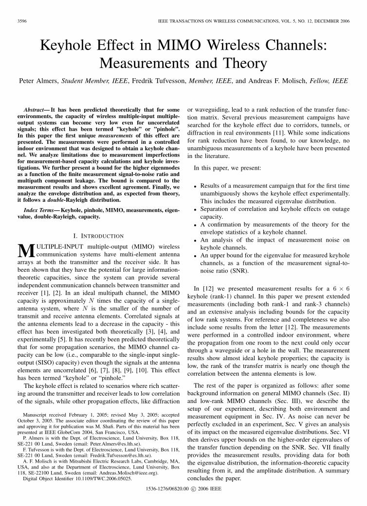
Fig. 1. Overview of the measurement setup.

Correlated MIMO channel snapshots can be generated fromboth the correlation matrix as

vec (Hfull) = R1/2·vec (Gfull) , (13)

and [3]

HKron =1

tr (RR)R1/2

R GKronRT/2T , (14)

where the former equation is generally valid, and the latter isvalid if the correlation matrix can be decomposed accordingto (10). Gfull and GKron are CN (0, I) distributed matricesof size NR × NT, and the matrix square root is defined asA1/2

(A1/2

)†= A.

The full correlation matrix is estimated from the measure-ments as

R =1M

M∑m=1

vec (H) · vec (H)† , (15)

and the marginal correlation matrices as

RR =1

MNT

M∑m=1

HmH†m, (16)

and

RT =1

MNR

M∑m=1

[H†

mHm

]T, (17)

where M denotes the number of different realizations.

B. Keyhole channels

As mentioned in the introduction, keyhole channels requirerich scattering environments around the two arrays withoutline-of-sight (LOS), together with a low rank connectionbetween the two scattering environments. Examples of keyholescenarios are

• Local rich scattering environments separated by a largedistance [10].

• Rich scattering environments connected by a rank-1propagation path, see Fig. 1 and [7], [12].

• Rich scattering environments connected via diffractionsover an edge.

Since the models in (14) and (13) only considers complexGaussian channels with spatial correlation, they cannot model

a keyhole2. In [10] a generalization of the Kronecker modelis presented

H =1√S

R1/2R GRT1/2GTR

T/2T , (18)

where GR and GT are both i.i.d. complex Gaussian matricesdistributed as CN (0, I), and where T1/2 describes the transfermatrix between the transmitter and receiver environments (i.e.,the scatterers around transmitter and receiver), and S is anormalization factor. For a perfect keyhole, e.g., a single-mode waveguide between the transmitter and the receiverenvironment, T1/2 has rank one. This results in a total channeltransfer matrix, H, of rank one as well, even though R1/2

R ,R1/2

T , GR and GT have full rank. The keyhole transfer matrixcan then be modeled as [8], [7]

Hkey = gRg†T, (19)

where gR,gT are column vectors distributed as,

gR,gT∈CN(0, σ2

keyI)

, and clearly the entries areuncorrelated [7].

When comparing the statistical properties of the entries inthe channel matrix of an i.i.d. and a keyhole channel, someinteresting differences are found.

• For i.i.d. channels the amplitudes of the entries in thetransfer matrix, H, are Rayleigh distributed, but show adouble-Rayleigh distribution for the keyhole channels:

f|hkey| (h) =h

σ4key

K0

(h

σ2key

), (20)

• The i.i.d. channel has uncorrelated and independent rowand column entries, whereas the keyhole channels hasuncorrelated but dependent row and column entries.

IV. KEYHOLE MEASUREMENT SETUP

To fulfill the keyhole scenario discussed in the previoussection, the measurements were performed with one antennaarray located inside a shielded chamber, and the other arrayin the adjacent room. A hole in the chamber wall was theonly propagation path between the two rooms. Fig. 1 showsthe layout of the measurement setup. The measurements wereperformed using a vector network analyzer (Rohde & SchwarzZVC at 3.5 − 4.0 GHz and a HP 8720C at 4.9 − 5.4 GHz).Linear virtual arrays with 6− 10 antenna positions and omni-directional conical antennas were used both at the transmitterand the receiver; the measurements were done during nighttime to ensure a static environment.

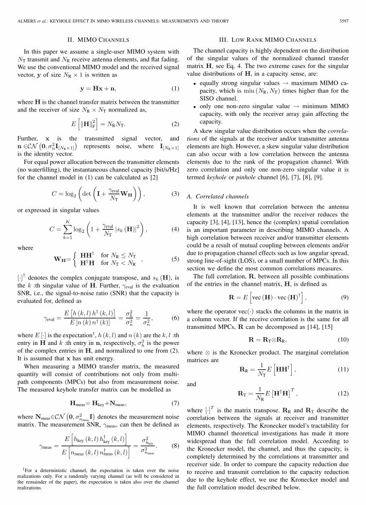
Two different rectangular waveguides were attached to thehole as in Fig. 2. The cut-off frequencies of a rectangularwaveguide are [17]

fco =1

2√

με

√(m

a

)2

+(n

b

)2

, (21)

where a is the width of the wave guide, b is the hight ofthe waveguide and m, n designate the mode. Further, μ and

2In the case of a keyhole, the instantaneous correlation [16] will be ableto predict a keyhole. However, the correlation used for the Kronecker modelis the mean correlation and is not able to predict the keyhole channel. It willtherefore overestimate the capacity for MIMO keyhole channels.


Fig. 2. Photo of the waveguide attached to the shielded chamber.

4 4.5 5 5.5 60

10

20

30

40

50

60

Frequency [GHz]

WG−II/WG−III

2.5 3 3.50

20

40

60

80

100

120

140

160

180

Frequency [GHz]

Mod

e at

tenu

atio

n [d

B]

WG−I

m=1 n=0m=2 n=0m=0 n=1m=1 n=1

m=1 n=0m=2 n=0m=0 n=1m=1 n=1

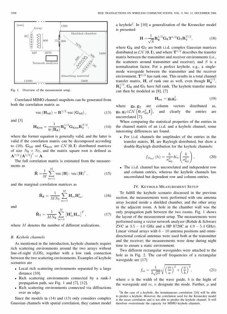
Fig. 3. Propagating mode attenuation.

ε are the absolute permeability and the absolute permittivityof the material filling the waveguide (air). The attenuation ofa propagating mode is theoretically zero at frequencies abovethat mode’s cut-off frequency, fco. Below the cut-off frequencythere is no true propagation but only significant attenuation.It is dependent on the length of the wave guide, z, and thefrequency distance to the cut-off frequency of that mode. Theattenuation is in the order of ∼ e−δ(f)z where [17]

δ (f) = h

√1 −

(f

fco

)2

, (22)

and

h =

√(mπ

a

)2

+(nπ

b

)2

. (23)

In Fig. 3 the attenuation of the first four propagating modesof the two different wave guides are plotted, where TE10 isf co = 3.19 GHz and fco = 2.59 GHz for WG-I and WG-II/WG-III, respectively. Note that the cut-off frequency, fco,are the same for (m = 2, n = 0) and (m = 0, n = 1) for WG-II/WG-III.

Two additional hole configurations without waveguideswere also measured. This gives us the following five setups:

1) A hole of size 47 × 22 mm with a 250 mm longwaveguide attached. We measured 101 complex transferfunctions at 3.5− 4 GHz, separated by 5 MHz spacing(referred to as WG-I).

2) A hole of size 58 × 29 mm with a 150 mm longwaveguide attached. We measured 51 complex transferfunctions at 3.5−4 GHz, separated by 10 MHz spacing(referred to as WG-II).

3) A hole of size 58 × 29 mm with a 150 mm longwaveguide attached. We measured 51 complex transferfunctions at 4.9 − 5.4 GHz, separated with 10 MHz(referred to as WG-III).

4) A hole of size 47 × 22 mm without waveguide, 101complex transfer functions separated with 5 MHz at3.5 − 4 GHz were taken (”small hole” or SH).

5) A hole of size 300 × 300 mm without waveguide, 101complex transfer functions separated with 5 MHz at3.5 − 4 GHz were taken (”large hole” or LH).

This means that as the measurement frequency increases inthe WG-III measurements, the waveguide shows a transitionfrom a one-moded wave guide to a three-moded waveguideaccording to Fig. 3.

The received signal was amplified by 30 dB with an externallow noise power amplifier to achieve a high measurementSNR. The measurement SNR was estimated to be 26 dBand 21 dB for WG-I and WG-II, respectively, where noiseincludes thermal noise, interference and possible channelchanges during the measurements. The large hole is intendedas test measurement, in which we do not anticipate a keyholeeffect but rather a full rank channel.

V. EFFECT OF MEASUREMENT NOISE ON

CHANNEL CAPACITY

In this section we analyze the influence of the nonidealityof measured transfer functions when calculating the capacity[18], and analyze its effect on our experiment. For keyholemeasurements, the measured transfer matrix normally consistsof the nominal keyhole transfer matrix, MPC leakage, andnoise, so that it can be modelled as in (7) with Nmeas alsoincludes the leakage components as

Nmeas = Hleak + N, (24)

where N ∈CN (0, σ2

n I)

denotes thermal noise. The MPCleakage describes MPCs propagating between the transmitterand the receiver via other paths than through the keyhole. Theleakage matrix together with non-static channel effect (varia-tions of the channel during the measurement time) is modelledby a complex Gaussian matrix Hleak∈CN

(0, σ2

hleakI). Using

a worst-case scenario (with respect to the resulting deviationfrom the capacity of an ideal keyhole channel), it is assumedto have independent entries.

Under these assumptions the noise leads to the same de-struction of the keyhole effect as leakage. In order to check theeffect on the evaluated capacity, we lump the two terms into asingle matrix as in (24). Assuming that Hkey, Hleak and N in(7) and (24) are independent, the measurement SNR (includingleakage) from a keyhole measurement point of view, γmeas, can


0 5 10 15 20 25 300

5

10

15

20

25

Evaluation SNR [dB]

50%

out

age

capa

city

[bit/

s/H

z]

sim., γmeas

= 20 dBWG−II, γ

meas = 21 dB

sim., γmeas

= 25 dBWG−I, γ

meas = 26 dB

sim., γmeas

= 30 dBsim., γ

meas = ∞ dB

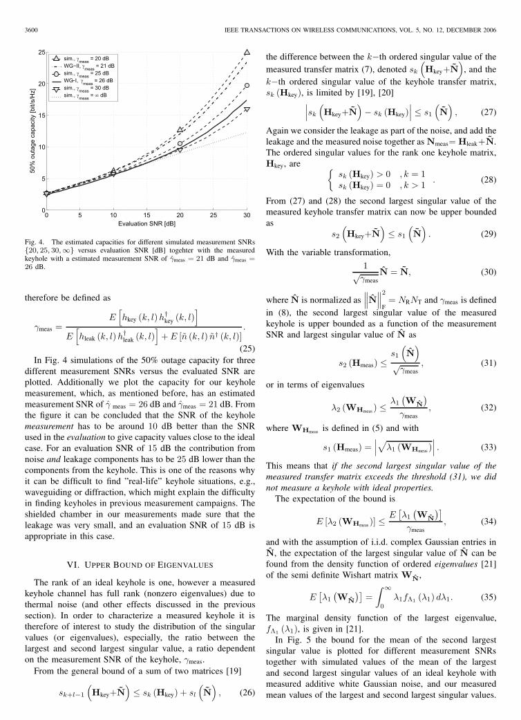
Fig. 4. The estimated capacities for different simulated measurement SNRs{20, 25, 30,∞} versus evaluation SNR [dB] togehter with the measuredkeyhole with a estimated measurement SNR of γmeas = 21 dB and γmeas =26 dB.

therefore be defined as

γmeas =E[hkey (k, l)h†

key (k, l)]

E[hleak (k, l)h†

leak (k, l)]

+ E [n (k, l) n† (k, l)].

(25)In Fig. 4 simulations of the 50% outage capacity for three

different measurement SNRs versus the evaluated SNR areplotted. Additionally we plot the capacity for our keyholemeasurement, which, as mentioned before, has an estimatedmeasurement SNR of γ meas = 26 dB and γmeas = 21 dB. Fromthe figure it can be concluded that the SNR of the keyholemeasurement has to be around 10 dB better than the SNRused in the evaluation to give capacity values close to the idealcase. For an evaluation SNR of 15 dB the contribution fromnoise and leakage components has to be 25 dB lower than thecomponents from the keyhole. This is one of the reasons whyit can be difficult to find ”real-life” keyhole situations, e.g.,waveguiding or diffraction, which might explain the difficultyin finding keyholes in previous measurement campaigns. Theshielded chamber in our measurements made sure that theleakage was very small, and an evaluation SNR of 15 dB isappropriate in this case.

VI. UPPER BOUND OF EIGENVALUES

The rank of an ideal keyhole is one, however a measuredkeyhole channel has full rank (nonzero eigenvalues) due tothermal noise (and other effects discussed in the previoussection). In order to characterize a measured keyhole it istherefore of interest to study the distribution of the singularvalues (or eigenvalues), especially, the ratio between thelargest and second largest singular value, a ratio dependenton the measurement SNR of the keyhole, γmeas.

From the general bound of a sum of two matrices [19]

sk+l−1

(Hkey+N

)≤ sk (Hkey) + sl

(N)

, (26)

the difference between the k−th ordered singular value of themeasured transfer matrix (7), denoted sk

(Hkey+N

), and the

k−th ordered singular value of the keyhole transfer matrix,sk (Hkey), is limited by [19], [20]∣∣∣sk

(Hkey+N

)− sk (Hkey)

∣∣∣ ≤ s1

(N)

, (27)

Again we consider the leakage as part of the noise, and add theleakage and the measured noise together as Nmeas= Hleak+N.The ordered singular values for the rank one keyhole matrix,Hkey, are {

sk (Hkey) > 0 , k = 1sk (Hkey) = 0 , k > 1 . (28)

From (27) and (28) the second largest singular value of themeasured keyhole transfer matrix can now be upper boundedas

s2

(Hkey+N

)≤ s1

(N)

. (29)

With the variable transformation,

1√γmeas

N = N, (30)

where N is normalized as∥∥∥N∥∥∥2

F= NRNT and γmeas is defined

in (8), the second largest singular value of the measuredkeyhole is upper bounded as a function of the measurementSNR and largest singular value of N as

s2 (Hmeas) ≤s1

(N)

√γmeas

, (31)

or in terms of eigenvalues

λ2 (WHmeas ) ≤λ1

(WN

)γmeas

, (32)

where WHmeas is defined in (5) and with

s1 (Hmeas) =∣∣∣√λ1 (WHmeas )

∣∣∣ . (33)

This means that if the second largest singular value of themeasured transfer matrix exceeds the threshold (31), we didnot measure a keyhole with ideal properties.

The expectation of the bound is

E [λ2 (WHmeas)] ≤E[λ1

(WN

)]γmeas

, (34)

and with the assumption of i.i.d. complex Gaussian entries inN, the expectation of the largest singular value of N can befound from the density function of ordered eigenvalues [21]of the semi definite Wishart matrix WN,

E[λ1

(WN

)]=∫ ∞

0

λ1fΛ1 (λ1) dλ1. (35)

The marginal density function of the largest eigenvalue,fΛ1 (λ1), is given in [21].

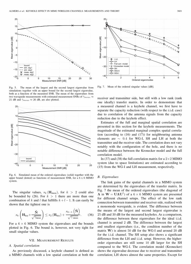
In Fig. 5 the bound for the mean of the second largestsingular value is plotted for different measurement SNRstogether with simulated values of the mean of the largestand second largest singular values of an ideal keyhole withmeasured additive white Gaussian noise, and our measuredmean values of the largest and second largest singular values.


−5 0 5 10 15 20 25 30−20

−15

−10

−5

0

5

10

15

20

Measurement SNR [dB]

Mea

n ei

genv

alue

[dB

]

boundsim. eig. 1sim. eig. 2meas. eig. 1meas. eig. 2

Fig. 5. The mean of the largest and the second largest eigenvalue fromsimulations together with an upper bound for the second largest eigenvalue,both as a function of the measured SNR. The mean of the eigenvalues fromtwo waveguide measurements with estimated measurement SNRs of γmeas ≈21 dB and γmeas ≈ 26 dB, are also plotted.

−5 0 5 10 15 20 25−40

−30

−20

−10

0

10

20

Measurement SNR [dB]

Mea

n ei

genv

alue

[dB

]

boundsimulation

Fig. 6. Simulated mean of the ordered eigenvalues (solid) together with theupper bound (dotted) as functions of measurement SNR, for a 6 x 6 MIMOsystem.

The singular values, sk (Hmeas), for k > 2 could alsobe bounded by (26). For k > 1 there are more than onecombination of k and l that fullfills k + l− 1. It can easily beshown that the tightest one is

sk

(Hkey+

N√γmeas

)≤ s2 (Hkey) +

sk−1

(N)

√γ meas

. (36)

For a 6 × 6 MIMO system the eigenvalues and the boundsplotted in Fig. 6. The bound is, however, not very tight forsmall singular values.

VII. MEASUREMENT RESULTS

A. Spatial correlation

As previously discussed, a keyhole channel is defined asa MIMO channels with a low spatial correlation at both the

1 2 3 4 5 6−40

−30

−20

−10

0

10

20

Ordered eigenmodes

Mea

n ei

genv

alue

[dB

]

i.i.d.LHFull corr. modelKronecker modelSHWG−IIWG−I

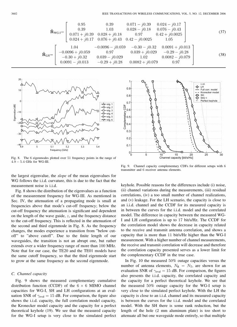
Fig. 7. Mean of the ordered singular values [dB].

receiver and transmitter side, but still with a low rank (rankone ideally) transfer matrix. In order to demonstrate thata measured channel is a keyhole channel, we first have toseparate the capacity reduction (with respect to the i.i.d. case)due to correlation of the antenna signals from the capacityreduction due to the keyhole effect.

Estimates of the full and marginal spatial correlation arepresented in this section for the keyhole measurements. Themagnitude of the estimated marginal complex spatial correla-tion (according to (16) and (17)) for neighbouring antennaelements are ∼ 0.4 for WG-I, SH and LH at both thetransmitter and the receiver side. The correlation does not varynotably with the configuration of the hole, and there is nonotable difference between the Kronecker model and the fullcorrelation model.

In (37) and (38) the full correlation matrix for a 2×2 MIMOsystem (due to space limitations) are estimated according to(15) from the WG-I and LH measurement, respectively.

B. Eigenvalues

The link gains of the spatial channels in a MIMO systemare determined by the eigenvalues of the transfer matrix. InFig. 7 the mean of the ordered eigenvalues (the diagonal ofΛ in W = UΛU†) of a 6 × 6 MIMO system are presentedfor different channel setups. The effect of the low rankconnection between transmitter and receiver side, realized witha monomode waveguide, is evident. The difference betweenthe means of the largest and second largest eigenvalue is25 dB and 30 dB for the measured keyholes. As a comparison,the difference between these eigenvalues for the ideal i.i.d.channel is around 2 dB. The difference between the largestand smallest eigenvalues (i.e., the condition number of thematrix W) is almost 50 dB for the WG-I and around 20 dBfor the i.i.d. channel. The SH setup also shows a significantdifference from the LH and i.i.d. setup. However, the higher-order eigenvalues are still some 10 dB larger for the SHcompared to the WG-I. The correlation model (Kronecker)shows the eigenvalue decrease due to receiver and transmittercorrelation; LH shows almost the same properties. Except for


RWG-I=

⎡⎢⎢⎣

0.95 0.39 0.071 − j0.39 0.024− j0.170.39 1.03 0.028 − j0.18 0.076− j0.43

0.071 + j0.39 0.028 + j0.18 0.97 0.42 + j0.00250.024 + j0.17 0.076 + j0.43 0.42 − j0.0025 1.05

⎤⎥⎥⎦ (37)

RLH=

⎡⎢⎢⎣

1.04 −0.0096− j0.059 −0.30 − j0.32 0.0091 + j0.013−0.0096 + j0.059 0.97 0.039 + j0.029 −0.29− j0.28−0.30 + j0.32 0.039− j0.029 1.02 0.0082− j0.079

0.0091− j0.013 −0.29 + j0.28 0.0082 + j0.079 0.97

⎤⎥⎥⎦ (38)

4.9 5 5.1 5.2 5.3 5.4−40

−30

−20

−10

0

10

20

Frequency [GHz]

Eige

nval

ue [d

B] eig. 1eig. 2eig. 3eig. 4eig. 5eig. 6

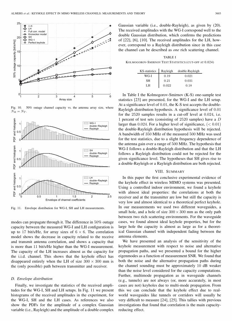
Fig. 8. The 6 eigenmodes plotted over 51 frequency points in the range of4.9 − 5.4 GHz for WG-III.

the largest eigenvalue, the slope of the mean eigenvalues forWG follows the i.i.d. curvature, this is due to the fact that themeasurement noise is i.i.d.

Fig. 8 shows the distribution of the eigenvalues as a functionof the measurement frequency for WG-III. As mentioned inSec. IV, the attenuation of a propagating mode is small atfrequencies above that mode’s cut-off frequency; below thecut-off frequency the attenuation is significant and dependenton the length of the wave guide, z, and the frequency distanceto the cut-off frequency. This is reflected in the attenuation ofthe second and third eigenmode in Fig. 8. As the frequencychanges, the modes experience a transition from ”below cut-off” to ”above cutoff”. Due to the finite length of ourwaveguides, the transition is not an abrupt one, but ratherextends over a wider frequency range of more than 100 MHz.Note that for our case, the TE20 and the TE01 models havethe same cutoff frequency, so that the third eigenmode startto grow at the same frequency as the second eigenmode.

C. Channel capacity

Fig. 9 shows the measured complementary cumulativedistribution function (CCDF) of the 6 × 6 MIMO channelcapacities for WG-I, SH and LH configurations at an eval-uation SNR of γeval = 15 dB. For comparison, the figure alsoshows the i.i.d. capacity, the full correlation model capacity,the Kronecker model capacity and the capacity for a perfecttheoretical keyhole (19). We see that the measured capacityfor the WG-I setup is very close to the simulated perfect

0 5 10 15 20 25 300

0.1

0.2

0.3

0.4

0.5

0.6

0.7

0.8

0.9

1

Channel capacity [bit/s/Hz]

Com

plem

etar

y C

DF

i.i.d.LHFull corr. modelKronecker modelSHWG−IPerfect keyhole

Fig. 9. Channel capacity complementary CDFs for different setups with 6transmitter and 6 receiver antenna elements.

keyhole. Possible reasons for the differences include (i) noise,(ii) channel variations during the measurements, (iii) residualcorrelations, (iv) a too small number of channel realizations,and (v) leakage. For the LH scenario, the capacity is close toan i.i.d. channel and the CCDF for its measured capacity isin between the curves for the i.i.d. model and the correlatedmodel. The difference in capacity between the measured WG-I and LH configuration is up to 17 bit/s/Hz. The CCDF forthe correlation model shows the decrease in capacity relatedto the receive and transmit antenna correlation, and shows acapacity that is more than 11 bit/s/Hz higher than the WG-Imeasurement. With a higher number of channel measurements,the receive and transmit correlation will decrease and thereforethe correlation capacity presented serves as a lower limit forthe complementary CCDF in the true case.

In Fig. 10 the measured 50% outage capacities versus thenumber of antenna elements, NR = NT, are shown for anevaluation SNR of γeval = 15 dB. For comparison, the figuresalso presents the i.i.d. capacity, the correlated capacity andthe capacity for a perfect theoretical keyhole. We see thatthe measured 50% outage capacity for the WG-I setup isvery close to the simulated perfect keyhole. With the LH thecapacity is close to an i.i.d. channel and its measured capacityis between the curves for the i.i.d. model and the correlatedmodel. With the SH there is some rank reduction, but thelength of the hole (2 mm aluminum plate) is too short toattenuate all but one waveguide mode entirely, so that multiple


1 2 3 4 5 60

5

10

15

20

25

Array size

50%

out

age

capa

city

[bit/

s/H

z]

i.i.d.LHFull corr. modelKronecker modelSHWG−IPerfect keyhole

Fig. 10. 50% outage channel capacity vs. the antenna array size, whereNR = NT .

0

0.5

1

PD

F an

d hi

stog

ram

WG−Idouble−RayleighRayleigh

0

0.5

1

PD

F an

d hi

stog

ram

SHdouble−RayleighRayleigh

0 0.5 1 1.5 2 2.50

0.5

1

Envelope of channel coefficients

PD

F an

d hi

stog

ram

LHdouble−RayleighRayleigh

Fig. 11. Envelope distribution for WG-I, SH and LH measurements.

modes can propagate through it. The difference in 50% outagecapacity between the measured WG-I and LH configuration isup to 17 bit/s/Hz, for array sizes of 6 × 6. The correlationmodel shows the decrease in capacity related to the receiveand transmit antenna correlation, and shows a capacity thatis more than 11 bit/s/Hz higher than the WG-I measurement.The capacity of the LH increases almost as the capacity forthe i.i.d. channel. This shows that the keyhole effect hasdisappeared entirely when the LH of size 300 × 300 mm isthe (only possible) path between transmitter and receiver.

D. Envelope distribution

Finally, we investigate the statistics of the received ampli-tudes for the WG-I, SH and LH setups. In Fig. 11 we presenthistograms of the received amplitudes in the experiment, forthe WG-I, SH and the LH cases. As references we alsoshow the PDFs for the amplitude of a complex Gaussianvariable (i.e., Rayleigh) and the amplitude of a double complex

Gaussian variable (i.e., double-Rayleigh), as given by (20).The received amplitudes with the WG-I correspond well to thedouble Gaussian distribution, which confirms the predictionsof [22], [6], [10]. The received amplitudes for the LH, how-ever, correspond to a Rayleigh distribution since in this casethe channel can be described as one rich scattering channel.

TABLE I

KOLMOGOROV-SMIRNOV TEST STATISTICS (CUT-OFF AT 0.024)

KS-statistics Rayleigh double-Rayleigh

WG-I 0.19 0.021

SH 0.21 0.031

LH 0.022 0.18

In Table I the Kolmogorov-Smirnov (K-S) one-sample teststatistics [23] are presented, for the WG-I and the LH setup.At a significance level of 0.01, the K-S test accepts the double-Rayleigh distribution hypothesis. A significance level of 0.01for the 2520 samples results in a cut-off level at 0.024, i.e.1 percent of test sets (consisting of 2520 samples) have a Dlarger than 0.024. For a higher level of significance, (< 0.01)the double-Rayleigh distribution hypothesis will be rejected.A bandwidth of 350 MHz of the measured 500 MHz was usedfor the test statistics, due to a slight frequency dependence ofthe antenna gain over a range of 500 MHz. The hypothesis thatWG-I follows a double-Rayleigh distribution and that the LHfollows a Rayleigh distribution could not be rejected for thegiven significance level. The hypotheses that SH gives rise toa double-Rayleigh or a Rayleigh distribution are both rejected.

VIII. SUMMARY

In this paper the first conclusive experimental evidence ofthe keyhole effect in wireless MIMO systems was presented.Using a controlled indoor environment, we found a keyholewith almost ideal properties: the correlations at both thereceiver and at the transmitter are low but still the capacity isvery low and almost identical to a theoretical perfect keyhole.In our measurements we used two different waveguides, asmall hole, and a hole of size 300× 300 mm as the only pathbetween two rich scattering environments. For the waveguidecases, we found almost ideal keyhole properties, but for thelarge hole the capacity is almost as large as for a theoret-ical Gaussian channel with independent fading between theantenna elements.

We have presented an analysis of the sensitivity of thekeyhole measurement with respect to noise and alternativepropagation paths, and we presented a bound for the highereigenmodes as a function of measurement SNR. We found thatboth the noise and the alternative propagation paths duringthe channel sounding must be approximately 10 dB weakerthan the noise level considered for the capacity computations.Further, multimode propagation as in waveguide channels(e.g., tunnels) are not always (or, more accurately, in mostcases are not) keyholes due to multi-mode propagation. Fromthis we can conclude that the keyhole effect due to real-world waveguides like tunnels or corridors will usually bevery difficult to measure [24], [25]. This tallies with previousinvestigations that found that correlation is the main capacity-reducing effect.


ACKNOWLEDGEMENT

Part of this work was financed by an INGVAR grant fromthe Swedish Foundation for Strategic Research.

REFERENCES

[1] J. H. Winters, “On the capacity of radio communications systemswith diversity in Rayleigh fading environments,” IEEE J. Sel. AreasCommun., vol. 5, pp. 871-878, June 1987.

[2] G. J. Foschini and M. J. Gans, “On limits of wireless communications infading environments when using multiple antennas,” Wireless PersonalCommun., vol. 6, pp. 311-335, 1998.

[3] D. Shiu, G. J. Foschini, M. J. Gans, and J. M. Kahn, “Fading correlationand its effect on the capacity of multi-element antenna systems,” IEEETrans. Commun., vol. 48, pp. 502-513, Mar. 2000.

[4] C. N. Chuah, D. N. C. Tse, J. M. Kahn, and R. A. Valenzuela, “Capacityscaling in MIMO wireless systems under correlated fading,” IEEE Trans.Inf. Theory, vol. 48, pp. 637-650, Mar. 2002.

[5] A. F. Molisch, M. Steinbauer, M. Toeltsch, E. Bonek, and R. S. Thoma,“Capacity of MIMO systems based on measured wireless channels,”IEEE J. Sel. Areas Commun., vol. 20, pp. 561-569, Apr. 2002.

[6] D. Chizhik, G. J. Foschini, and R. A. Valenzuela, “Capacities ofmultielement transmit and receive antennas: correlations and keyholes,”IEEE Electron. Lett., vol. 36, pp. 1099-1100, June 2000.

[7] S. Loyka and A. Kouki, “On MIMO channel capacity, correlations, andkeyholes: analysis of degenerate channels,” IEEE Trans. Commun., vol.50, pp. 1886-1888, Dec. 2002.

[8] D. Gesbert, H. Blcskei, D. A. Gore, and A. J. Paulraj, “MIMOwireless channels: capacity and performance prediction,” in Proc. IEEEGLOBECOM 2000, vol. 2, pp. 1083-1088.

[9] D. Chizhik, G. J. Foschini, M. J. Gans, and R. A. Valenzuela, “Key-holes, correlations, and capacities of multielement transmit and receiveantennas,” IEEE Trans. Commun., vol. 1, pp. 361-368, Apr. 2002.

[10] D. Gesbert, H. Blcskei, D. A. Gore, and A. J. Paulraj, “Outdoor MIMOwireless channels: models and performance prediction,” IEEE Trans.Commun., vol. 50, pp. 1926-1934, Dec. 2002.

[11] D. Chizhik, J. Ling, P. W. Wolniansky, R. A. Valenzuela, N. Costa, andK. Huber, “Multiple-input-multiple-output measurements and modelingin manhattan, IEEE J. Sel. Areas Commun., vol. 21, pp. 321-331, Apr.2003.

[12] P. Almers, F. Tufvesson, and A. F. Molisch, “Measurement of keyholeeffect in a wireless multiple-input multiple-output (MIMO) channel,”IEEE Commun. Lett., vol. 7, pp. 373-375, Aug. 2003.

[13] R. R. Mueller, “A random matrix model of communication via antennaarrays,” IEEE Trans. Inf. Theory, vol. 48, pp. 2495-2506, Sept. 2002.

[14] C. Oestges, B. Clerckx, D. Vanhoenacker-Janvier, and A. Paulraj,“Impact of diagonal correlations on mimo capacity: application togeometrical scattering models, in Proc. IEEE VTC 2003/Fall, vol. 1,pp. 394-398.

[15] K. Yu, “Modeling of multiple-input multiple-output radio propagationchannels,” Licentiate Thesis, July 2002, KTH, Sweden.

[16] S. Loyka and A. Kouki, “New compound upper bound on MIMOchannel capacity,” IEEE Commun. Lett., vol. 6, pp. 96-98, Mar. 2002.

[17] D. K. Cheng, Field and Wave Electromagnetics, Second Edition. Addi-son.Wesley, 1989.

[18] P. Kyritsi, R. A. Valenzuela, and D. C. Cox, “Channel and capacityestimation errors,” IEEE Commun. Lett., vol. 6, pp. 517-519, Dec. 2002.

[19] R. A. Horn and C. R. Johnson, Topix in Matrix Analysis. London:Cambridge University Press, 1991.

[20] G. H. Golub and C. F. V. Loan, Matrix Computations, Second Edition.London: Johns Hopkins University Press, 1989.

[21] I. E. Telatar, “Capacity of multi-antenna Gaussian channels,” EuropeanTrans. Telecommun., vol. 10, Nov./Dec. 1999.

[22] V. Erceg, S. J. Fortune, J. Ling, A. J. R. Jr., and R. A. Valenzuela,“Comparisons of a computer-based propagation prediction tool withexperimental data collected in urban microcellular environments,” IEEEJ. Sel. Areas Commun., vol. 15, pp. 677-684, May 1997.

[23] F. J. Massey, The Kolmogorov-Smirnov test for goodness of t,” J.American Statistical Association, vol. 46, pp. 68-78, Mar. 1951.

[24] S. Loyka, “Multiantenna capacities of waveguide and cavity channels,”in Proc. IEEE CCECE 2003, vol. 3, pp. 1509-1514.

[25] S. Loyka, “Multiantenna capacities of waveguide and cavity channels,IEEE Trans. Veh. Technol., vol. 54, pp. 863-872, May 2005.

Peter Almers received the M.S. degree in elec-trical engineering in 1998 from Lund Universityin Sweden. In 1998, he joined the radio researchdepartment at TeliaSonera AB (formerly Telia AB),in Malmo, Sweden, mainly working with WCDMAand 3GPP standardization physical layer issues. Pe-ter is currently working towards the Ph.D. degree atthe Department of Electroscience, Lund University.He has participated in the European research ini-tiatives COST273, and is currently involved in theEuropean network of excellence “NEWCOM” and

the NORDITE project “WILATI.” Peter received an IEEE Best Student PaperAward at PIMRC in 2002.

Fredrik Tufvesson was born in Lund, Sweden in1970. He received the M.S. degree in ElectricalEngineering in 1994, the Licentiate Degree in 1998and his Ph.D. in 2000, all from Lund Universityin Sweden. After almost two years at a startupcompany, Fiberless Society, Fredrik is now asso-ciate professor at the department of Electroscienceworking on channel measurements and modeling forMIMO and UWB systems. His research interestsalso include channel estimation and synchronizationproblems for wireless communication, especially for

wireless OFDM systems.

Andreas F. Molisch (S’89, M’95, SM’00, F’05)received the Dipl. Ing., Dr. techn., and habilitationdegrees from the Technical University Vienna (Aus-tria) in 1990, 1994, and 1999, respectively. From1991 to 2000, he was with the TU Vienna, becomingan associate professor there in 1999. From 2000-2002, he was with the Wireless Systems ResearchDepartment at AT&T (Bell) Laboratories Researchin Middletown, NJ. Since then, he has been withMitsubishi Electric Research Labs, Cambridge, MA.He is also professor and chairholder for radio sys-

tems at Lund University, Sweden.Dr. Molisch has done research in the areas of SAW filters, radiative

transfer in atomic vapors, atomic line filters, smart antennas, and widebandsystems. His current research interests are MIMO systems, measurement andmodeling of mobile radio channels, cooperative communications, and UWB.Dr. Molisch has authored, co-authored or edited four books (among them therecent textbook Wireless Communications, Wiley-IEEE Press), eleven bookchapters, some 95 journal papers, and numerous conference contributions.

Dr. Molisch is an editor of the IEEE Transactions on Wireless Commu-nications, co-editor of a recent special issue on MIMO and smart antennasin the Journal of Wireless Communications and Mobile Computing, and co-editor of a recent special issue on UWB in IEEE Journal on Selected Areasin Communications.

He has been member of numerous TPCs, vice chair of the TPC of VTC2005 spring, and will be general chair of ICUWB 2006. He has participatedin the European research initiatives COST 231, COST 259, and COST273,where he was chairman of the MIMO channel working group, and is alsochairman of Commission C (signals and systems) of URSI (InternationalUnion of Radio Scientists). Dr. Molisch is a Fellow of the IEEE and recipientof several awards.

keyhole effect in mimo wireless channels: measurements and theory

Documents