X. Zhao et al.Int. J. Environ. Sci. Tech., 8 (1), 137-148, Winter 2011ISSN: 1735-1472© IRSEN, CEERS, IAU

*Corresponding Author Email: zyshen@bnu.edu.cn Tel.: +8610 5880 0398; Fax: +8610 5880 0398

Received 7 July 2010; revised 5 October 2010; accepted 24 November 2010; available online 1 December 2010

Key uncertainty sources analysis of water quality model using the first order error method

1X. Zhao; 1*Z. Y. Shen; 2M. Xiong; 3J. Qi

1State Key Laboratory of Water Environment Simulation, School of Environment, Beijing Normal University, Beijing 100875, P. R. China

2Bureau of Hydrology, Changjiang Water Resources Commission, Wuhan, Hubei Province 430010,

P. R. China

3Beijing Municipal Research Institute of Environmental Protection, Beijing 100037, P. R. China 

ABSTRACT: In this study, key uncertainty sources analysis was undertaken for a dynamic water model using a Firstorder error analysis method. First, a dynamic water quality model for the Three Gorges Reservoir Regions wasestablished using data after impoundment by the environmental fluid dynamics code model package. Model calibrationand verification were then conducted using measured data collected during 2004 and 2006. Four statistical indices wereemployed to assess the modeling efficiency. The results indicated that the model simulated the variables well, with mostrelative error being less than 25 %. Next, input and parameter uncertainty analysis were conducted for ammonianitrogen, nitrate nitrogen, total nitrogen, and dissolved oxygen at 3 grid cells located in the upper, middle and downstreamportions of the research area. For the nitrogen related variables, input from Zhutuo Station, the Jialingjiang River, andthe Wujiang River were the main sources of uncertainty. Point and nonpoint sources also accounted for a large ratio ofuncertainty. Moreover, nitrification contributed some uncertainty to the estimated ammonia nitrogen and nitrate nitrogen.However, reaeration was found to be a key source of uncertainty for dissolved oxygen, especially at the middle anddownstream reaches. The analysis conducted in this study gives a quantitative assessment for uncertainty sources ofeach variable, and provides guidance for further pollutant loading reduction in the Three Gorge Reservoir Region.

Key words: Dissolved oxygen; Environmental Fluid Dynamics Code; Model; Nitrogen; Water quality

INTRODUCTIONRecently, water quality models have been widely

employed worldwide for water environment assessmentand prediction in various water bodies including lakes,reservoirs, oceans, rivers and estuaries, a case in pointis oil spill model in estuaries water (Nagheeby andKolahdoozan, 2010; Kuok et al., 2010). Indeed, in theUnited States, water quality models have becomeessential tools for estimating the distribution of thetotal maximum daily load (TMDL) and developing bestmanagement practices (BMPs), (EPA, 2009; Turner etal., 2009; Iginosa and Okoh, 2009; Chen et al., 2010).The transport and fate of water quality constituents inthe water column are simulated using modelingmodules such as river and stream water Quality Model

(QUAL2K), (Chapra et al., 2007), water quality analysissimulation program (WASP) (Wool et al., 2001),environmental fluid dynamics code (EFDC) (Tetra Tech,2007)and MIKE11 (DHI, 2003), which describe theproblems related to chemical and biological processesthrough deterministic partial differential equations(Igwe et al., 2008; Shah et al., 2009). These models aredeterministic because they provide a single responsefor each set of parameters, initial and boundaryconditions (Bobba et al., 1996). However, there isalways uncertainty associated with models. In general,uncertainty comes from four aspects when modelingwater quality (Radwan et al., 2004): (I) structuraluncertainties; specifically, basic processesmathematically characterizing changes in variables inthe water column may not be always identical in

X. Zhao et al.

138

different models, and some processes may be ignoredor combined with others. For example, in the EFDCmodel (Tetra Tech, 2007), organic nitrogen is dividedinto refractory particulate organic nitrogen, liableparticulate organic nitrogen and dissolved organicnitrogen; however, in the WASP (Wool et al., 2001)model, it is a single variable; (II) parameter uncertainty;specifically, a set of parameters suitable for one modelmay be lower quality than in other models as a result ofdifferent climatic, topographic, and hydrodynamicconditions; (III) input uncertainty; specifically, futureloadings based on projections may be over or underestimated; and (IV) measurement uncertainty,measurement results are closely related to researcher’sexperiences and precision of instruments.

Many methods have been proposed to assess theuncertainty associated with various resourcesquantitatively, including the following: first order erroranalysis (FOEA), which is a procedure based on firstorder terms in the Taylor series expansion of thedependent variable around its mean value with respectto one or more independent variables (Bobba et al.,1996; Abrishamchi et al., 2005); Monte Carlo (Tomassiniand Reichert, 2007), which uses a large number ofsimulations with the values for stochastic inputs oruncertain variables being selected at random from theirassumed parent probability distributions to establishan expected range of model uncertainty; Markov ChainMonte Carlo, a modified MC method that includes theMarkov chain analysis (Tomassini and Reichert, 2007);generalized likelihood uncertainty estimation, whichworks with multiple sets of factors, typically via MonteCarlo sampling, and applies likelihood measures toestimate the predictive uncertainty of the model (Rattoand Saltelli, 2001; Soner Kara and Onut, 2010); pointestimation method (PEM), in which the probabilitydistribution function (PDF) of each random inputvariable is represented by a number Np of discretepoints located according to the first, second and thirdmoments of the PDF, and the joint PDF of Nparparameters is represented by the array of projectedpoints (Franceschini and Tsai, 2010).

For large, complex dynamic models with disperseparameter distributions, FOEA may be computationallyfeasible, and do not specify parameter distributions,which is an important issue to consider in methodssuch as MC. Unfortunately, the effect of differentchoices of distributions is difficult to assess (USEPA,1999). Furthermore, FOEA provides a very clear

approach to uncertainty analysis by decomposing thevariance of each output into the sum of contributionsfrom each input. Therefore it allows explicitconsideration of the combined effects of parametersensitivity and parameter uncertainty in thedetermination of the key parameters affecting model-prediction uncertainty and is easy to update the riskestimation when new information becomes available(Zhang and Yu, 2004). So, FOEA is a more suitable toolfor uncertainty analysis in the Three Gorges ReservoirRegion (TGRR). Modeling research has beenundertaken for more than 20 years in the TGRR. In1991, the Report on the Impact of the Three GorgesProject (TGP) on Ecology and the Environment wascompleted by the Changjiang Water ResourcesProtection Institute in cooperation with the ChineseAcademy of Sciences and other institutes. However,due to technical limitations, qualitative evaluation ofthe effects of water impoundment on water quality wasonly preliminarily conducted in this study, and only afew empirical formulas and simple mathematical modelswere used (Yu, 2008). From 1989 to 2001, the ChongqingEnvironmental Science Institute in cooperation withresearch institutes from the United Kingdom andDenmark launched a series of hydrodynamic and waterquality simulations in the Chongqing section of theTGRR using 2-D and quasi 2-D vertically mixed models.In their study, the chemical oxygen demand (COD),NH4-N, Biochemical oxygen demand (BOD5) and otherwater quality parameters were simulated; however,changes in the water environment throughout the entirereservoir were not considered.1 In 1996, a systemicresearch program known as the Water Pollution Controlin the Three Gorges Reservoir Area Program waslaunched by the Three Gorges Project ConstructionCommission of the State Council and several researchorganizations (Huang et al., 2006). Three topics wereincluded in this program: (1) identification of currentpollution loads and forecast of the pollution trend; (2)analysis of changes in water quality caused by waterimpoundment; and (3) assignment of the aquaticenvironmental capacity of pollutants to meet specifiedwater quality standards. To predict the waterenvironmental quality under different impoundmentconditions, a 1-D hydrodynamic and water qualitymodel was developed by the China Institute of WaterResources and Hydropower Research for the entirereservoir area, from the dam to about 660 km upstream(Liet al., 2002). However, due to restrictions in the basic

X. Zhao et al.

139

Int. J. Environ. Sci. Tech., 8 (1), 137-148, Winter 2011

data, the model does not take into account the impactof sediments and some biochemical processes had tobe simplified. For example, phosphorus was treated asa conservative substance in the model. In this study, alarge scale dynamic water quality model was providedfor the whole TGRR, and the modeling task has beenlasted about 10 months from March, 2008. Whencompared to previously conducted modeling practices,data from 2004 and 2006 were used to calibrate andvalidate the model, and these data can further reflectchanges in water quality after impoundment.Additionally, the latest measured point and nonpointsources data were used as important external sourcesof variables and the model kinetic processes were morecomplex than forgone models. Next, detailed input andparameter uncertainty analysis was conducted usingthe FOEA method because a great deal of uncertaintyanalysis in water quality modeling is grouped in staticand simple kinetic processes such as QUAL2E, whilethey are relatively rare for dynamic and complex modelsystems.

MATERIALS AND METHODSStudy Area

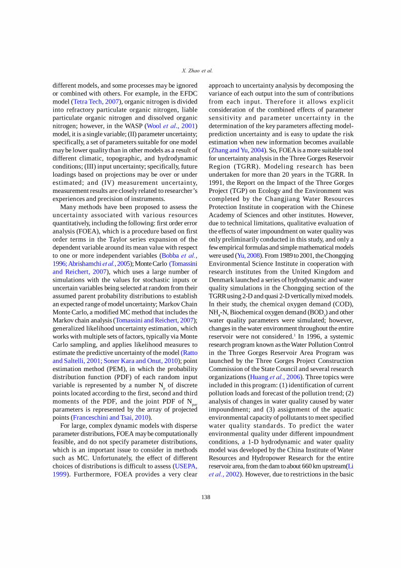
The TGRR ranges from Chongqing City to YichangCity, Hubei Province (106°16´~111°28´E,28°56´~31°44´N) (Fig. 1). This region refers to the area

affected by the water impoundment of the TGP andcovers an area of 54,000 km2 (Zhang et al., 2009). Mostof this area is mountainous, with the western portionhaving an elevation ranging from 1000 to 2500 m andthe eastern portion having an elevation of about 500 -900 m. The study area is subject to the tropical monsoonclimate of Northern Asia and has an annual meantemperature, precipitation, evaporation rate and windspeed of 18 °C, 1170 mm, 1300 mm and 1.4 m/s,respectively. In the TGRR, water is quite plentiful, withan average flow of 40.56 billion m3 per year, of whichunderground runoff accounts for about 21 %. However,the temporal and spatial distribution of water in theregion is very uneven and the Northwest is short ofwater during the spring and winter. There are more than200 tributaries with a drainage area that is greater than100 km2 in the TGRR, including the Jialing, Wujiangand Daninghe rivers (Deng, 2007).

Model DescriptionThe EFDC model package, which was originally

developed by John Hamrick at the Virginia Institute ofMarine Science (VIMS), is a general purpose three-dimensional modeling package for flow, pollutanttransport and biogeochemical processes in surfacewater systems including rivers, lakes, estuaries,reservoirs, wetlands and coastal regions(Tetra Tech,

Fig. 1: Location of monitoring stations in the TGRR

SitesBranchMain stream of the Yangtze RiverThe three Gorges Reservoir Region

0 50 100 200 km

Zhutuo

Beibei

Cuntan

Changshou

Qingxichang

Zhongxian

Wanzhou

FengjieWushan

BadongMiaohe

Legend

China

X. Zhao et al.

140

Uncertainty analysis of water quality model using first order error method

2007). The structure of the EFDC model includes fourmajor modules: (1) a hydrodynamic sub-model, (2) awater quality sub-model, (3) a sediment transport sub-model and (4) a toxics sub-model. The water columnwater quality model simulates the spatial and temporaldistributions of 21 state variables in the water column.For each state variable, a mass conservation equation(Eq. 1) is established:

( ) ( ) ( )

czyx SzCK

zyCK

yxCK

x

zCw

yCv

xCu

tC

+⎟⎠⎞

⎜⎝⎛

∂∂

∂∂

+⎟⎟⎠

⎞⎜⎜⎝

⎛∂∂

∂∂

+⎟⎠⎞

⎜⎝⎛

∂∂

∂∂

=∂

∂+

∂∂

+∂

∂+

∂∂

(1)

where C is the concentration of a water quality statevariable; u, v and w are the water velocity componentsin the x, y and z directions, respectively, and Kx, Ky andKz are the turbulent diffusivities in the x, y and zdirections, respectively. In addition, Sc represents theinternal and external sources and sinks of the waterquality state variable, which are those generated/consumed by kinetic processes. The kineticformulations in the model are primarily from CE-QUAL-ICM (Cerco and Cole, 1994).

Data PreparationIn this study, the basic data sets required to

develop the models included bathymetry, hydrology,meteorological data and water quality data. Atopographic map with a resolution of 1:25,000 wasused to delineate the channel characteristics, andbathymetry data collected from along the river wasobtained from the available literature (Huang et al.,2006). Hydrology and water quality data, includingthe DO, BOD5, NH4-N, NO3-N and TN, collected from2003 to 2007 at 12 monitoring stations in the researcharea were obtained from the Bureau of Hydrology,Changjiang Water Resources Commission.Meteorological data from 2003 to 2007 weredownloaded from the website maintained by theChingqing Meteorological Bureau. Industrial andmunicipal point pollution sources for each county anddistrict in 2002 in the TGRR were obtained from theChina Environmental Science Research Institute(CRAES), and data from 2004 to 2007 were obtainedfrom the Three Gorges Bulletins (MEP, 2010). Non-point source nutrient emission data were obtainedfrom Zhen et al. (2009).

Model Configuration, Calibration and ValidationSEAGRID (Denham, 2006) was applied to create

orthogonal curvilinear grids, while the GEFDC softwarewas used to create dxdy.inp and lxly.inp files(Tetra Tech,2007). For the initial condition, the water surface elevation(WSE) and water quality variables for each active cellwere interpolated based on monitoring data collectedalong the Changjiang River. For water variables, variousspecies of nitrogen and carbon were estimated accordingto Ji (2008) and field data. Zhutuo, Beibei and WulongStations were treated as the inflow boundary, while theopen boundary was the downstream area of the ThreeGorges Dam. Meteorological conditions were used asthe driving function for the model. Default parameterswere initially used to run the model and were lateradjusted during calibration with the data from 2004.Model validation was conducted using the data from2006. Simulation results were evaluated using 4 pre-defined statistics parameters: Average error (AE), Relativeerror (RE); Average absolute error (AAE) and Root meansquare error (RMSE).

FOEA methodIn FOEA, a function Y=f(X), was approximated by afirst order Taylor series expansion around the expectedX:

∑=

∂∂−+=p

i Xiieie eXYXXXYY

1)/)(()( (2)

where Y = the concentration of the constituentsimulated in the selected water quality model; Xe = thevector of uncertain basic variables representing theexpansion point; p= the number of basic variables Xi.The expansion point is commonly the mean value (orsome other convenient central value) of the basicvariables. Thus, the expected value and variance ofthe performance function can be expressed as follows:

)()(m

XYYE ≈ (3)

[ ])XX)(XX(E)X/Y(

)X/Y()Y(Var

jiimiimXj

p

1i

p

1i mXi2Y

−−∂∂

∑∑ ∂∂≈== =

σ (4)

whereσY =the standard deviation of Y; and Xm =thevector of mean values of the basic variables. If thebasic variables are statistically independent, thevariance of Y becomes

[ ]∑=

∂∂==p

i iiYXYYVar

1

22 )/()( σσ (5)where σi= the standard deviation of variables Xi.

X. Zhao et al.

141

Int. J. Environ. Sci. Tech., 8 (1), 137-148, Winter 2011

When 0→∆X , Equation (4) becomes

∑= ∆

∆=

P

ii

i XYXVarYVar

1

2))(()( (6)

Then

∑=

∆∆=

P

i

i

i YXYXVar

YYVar

1 2

2

2

)/()()( (7)

/

)/()()(1 22

2

22∑=

∆∆=

P

ii

i

i

i

XYXY

XXVar

YYVar

(8)

[ ] [ ]∑= ∆

∆=

P

iiii

i

XXYY

XX

Y 1 2

2

2

2

)

2

2

)/()/(((Y) σσ

(9)

[ ] [ ]∑= ⎥

⎦

⎤⎢⎣

⎡∆∆

=P

iii

i XXYYXCV

1

2

22

/()/()(SD(Y) (10)

[ ] [ ]∑=

=P

i iiSXCV

1

222 )()(SD(Y) (11)

where Var(Xi)=the variance of basic variables;SD(Y)=the standard deviation of the output;CV(X)=the coefficient of variation; Si=the normalizedsensitivity coefficient.

RESULTS AND DISCUSSIONModel Calibration and Verification

Based on the availability of the measured data, thedata obtained from the Cuntan, Qingxichang andWanzhou monitoring stations (Fig. 1) were selectedfor parameter calibration and verification. The modeled

Table 1: Simulated Results analysis in Cuntan, Qingxichang and Wanzhou Stations

2004 2006 Station ID Variable AE RE AAE RMS AE RE AAE RMS Cuntan WSE (m) -0.77 0.49 0.79 1.02 -0.14 0.63 1.01 8.31 Qingxichang WSE(m) 0.76 0.56 0.79 0.94 0.91 0.67 0.96 8.08 Wanzhou WSE (m) -0.4 0.29 0.4 0.65 -0.11 0.14 0.2 0.3 Cuntan Temperature (℃) -0.27 4.88 1.05 1.41 -0.28 4.96 1.05 1.36 Qingxichang Temperature (℃) -0.83 8.19 1.75 2.14 -0.74 6.01 1.29 1.61 Wanzhou Temperature (℃) -0.4 5.57 1.21 1.58 -0.3 5.67 1.23 1.59 Cuntan DO (g/m3) -0.22 5.97 0.54 0.64 1.73 23.3 1.73 1.78 Qingxichang DO (g/m3) -0.16 7.01 0.63 0.77 1.82 24.57 1.82 1.93 Wanzhou DO (g/m3) -0.17 5.84 0.47 0.59 0.53 8.65 0.68 0.78 Cuntan NH4-N (g/m3) 0.05 44.58 0.07 0.08 -0.02 24.48 0.05 0.07 Qingxichang NH4-N (g/m3) 0.01 42.56 0.07 0.09 0.01 17.56 0.03 0.04 Wanzhou NH4-N g/m3) -0.04 35.93 0.07 0.1 -0.03 24.64 0.06 0.07 Cuntan NO3-N (g/m3) -0.09 7.85 0.11 0.15 0.01 9.67 0.12 0.16 Qingxichang NO3-N (g/m3) -0.17 11.99 0.18 0.21 0.02 13.05 0.17 0.26 Wanzhou NO3-N (g/m3) -0.15 12.06 0.18 0.22 0.02 8.87 0.12 0.15 Cuntan TN (g/m3) 0.06 11.68 0.22 0.26 -0.1 13.55 0.24 0.42 Qingxichang TN (g/m3) 0.05 13.85 0.26 0.3 -0.14 0.63 1.01 8.31 Wanzhou TN (g/m3) 0.17 14.27 0.25 0.31 0.91 0.67 0.96 8.08

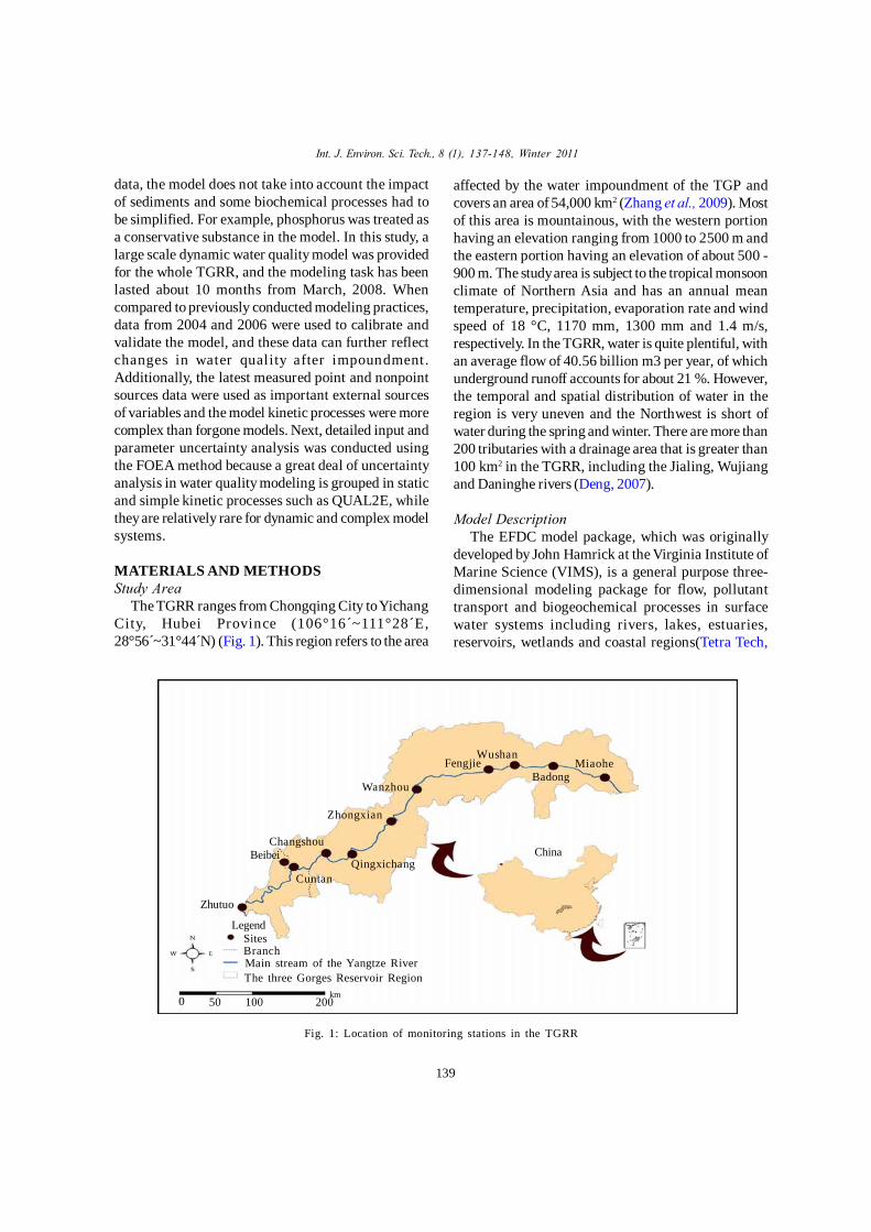
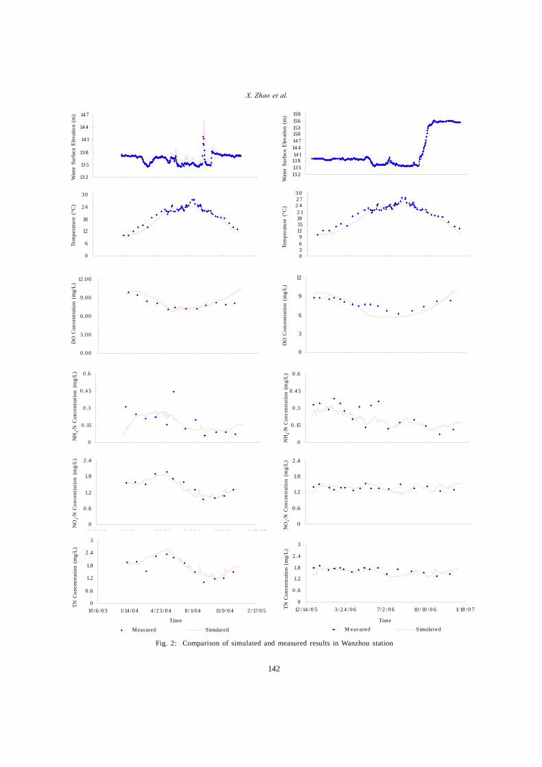
periods were 2004 and 2006. The time step was 60s, andit took about 1 h to complete model implementation.The simulation results were compared with measureddata as follows: a time series comparison at each station,a longitudinal profile comparison for the entire reservoirregion, and a statistical table (Table 1). For the purposeof simplicity, this paper only provides the time seriescomparison for Wanzhou Station.

Figs. 2a-f provide a comparison of results obtainedfor Wanzhou station during the calibration period. Fig.2a shows that the simulated and measured WSEmatched very well before and after the high flow period,and that the simulation results were slightly larger thanthe corresponding measured values during the highflow period. This may have been caused by abundantinflows from other ignored tributaries in the reservoirregion such as the Yulin River, the Zhuxi River and theXiaojiang River. These findings indicate that theextreme peak value of the measured data cannot alwaysbe reproduced in the modeling process. With respectto temperature (Fig. 2b), the computations are in goodagreement with the observed data. The DOconcentration is important for supporting the aquaticecosystem, and prolonged exposures to less than 60 %oxygen saturation may result in altered behavior, growthreduction, adverse reproductive effects and mortality.Fish will begin to feel stress when the DO drops toabout 4 mg/L and will swim away from areas in whichthe DO is below 3 mg/L. Fish that are unable to swimaway from such areas and shell fish will begin to die

X. Zhao et al.

142

Fig. 2: Comparison of simulated and measured results in Wanzhou station

Wat

er S

urfa

ce E

leva

tion

(m)

DO

Con

cent

ratio

n (m

g/L)

NH

4-N C

once

ntra

tion

(mg/

L)N

O3-N

Con

cent

ratio

n (m

g/L)

TN C

once

ntra

tion

(mg/

L)Te

mpe

ratu

re (

°C)

13 2

13 5

13 8

141

14 4

14 7

10 /6 /03 1/14 /04 4 /23 /0 4 8 /1/0 4 11/9 /04 2 /17/05

0

6

12

18

24

30

10 /6 /0 3 1/14 /04 4 /2 3 /0 4 8 /1/0 4 11/9 /04 2 /17/0 5

0 .00

3 .00

6 .00

9 .00

12 .00

10 /6 /0 3 1/14 /0 4 4 /23 /04 8 /1/0 4 11/9 /04 2 /17/05

0

0 .15

0 .3

0 .4 5

0 .6

10 / 6 / 0 3 1/ 14 / 0 4 4 / 2 3 /0 4 8 / 1/ 0 4 11/ 9 / 0 4 2 / 17/0 5

0

0 .6

1.2

1.8

2 .4

10 /6 /0 3 1/14 /0 4 4 /2 3 /0 4 8 /1/0 4 11/9 /0 4 2 /17/0 5

0

0 .6

1.2

1.8

2 .4

3

10 /6 /03 1/14 /04 4 /23 /0 4 8 /1/04 11/9 /04 2 /17/0 5

Measured Simulated

Time

Wat

er S

urfa

ce E

leva

tion

(m)

DO

Con

cent

ratio

n (m

g/L)

NH

4-N C

once

ntra

tion

(mg/

L)N

O3-N

Con

cent

ratio

n (m

g/L)

TN C

once

ntra

tion

(mg/

L)Te

mpe

ratu

re (

°C)

13 213 513 814 114 414 7150153156159

12 /14 /0 5 3 /2 4 /0 6 7/2 /0 6 10 /10 /0 6 1/18 /0 7

0369

1215182 1

2 42 73 0

12 / 14 / 0 5 3 /2 4 / 0 6 7/ 2 /0 6 10 /10 /0 6 1/ 18 / 0 7

0

3

6

9

12

12/14/05 3/24/06 7/2/06 10/10/06 1/18/07

0

0 .15

0 .3

0 .4 5

0 .6

12 /14 /0 5 3 /2 4 /0 6 7/2 /0 6 10 /10 /0 6 1/18 /0 7

0

0 .6

1.2

1.8

2 .4

12 /14 /0 5 3 /2 4 /0 6 7/2 /06 10 /10 /0 6 1/18 /07

0

0 .6

1.2

1.8

2 .4

3

12 /14 /0 5 3 / 2 4 / 0 6 7/2 / 0 6 10 / 10 /0 6 1/18 /0 7

M eas ured Simula tedTime

X. Zhao et al.Int. J. Environ. Sci. Tech., 8 (1), 137-148, Winter 2011

when the DO is below this level (Karim et al., 2002).The comparison plot in Fig. 2c indicates that themeasured change in DO concentration was duplicatedby the model. The change in the temporal NH4-Nconcentration was also represented by the model (Fig.2d), but larger discrepancies existed at some times,possibly due to the enormous variation in fieldmeasured data, which ranged from <0.1 mg/l duringthe low flow period to 0.45 mg/l in the high flow period.The NO3-N (Fig. 2e) and TN (Fig. 2f) showed the sametrend, which was likely because NO3-N accounts forthe highest ratio of the TN in the TGRR (Huang etal., 2006). The simulated NO3-N and TN were close tothe field data, which was probably due to the factthat the NO3-N concentration was less affected byexternal loads such as non-point sources during thehigh flow period.

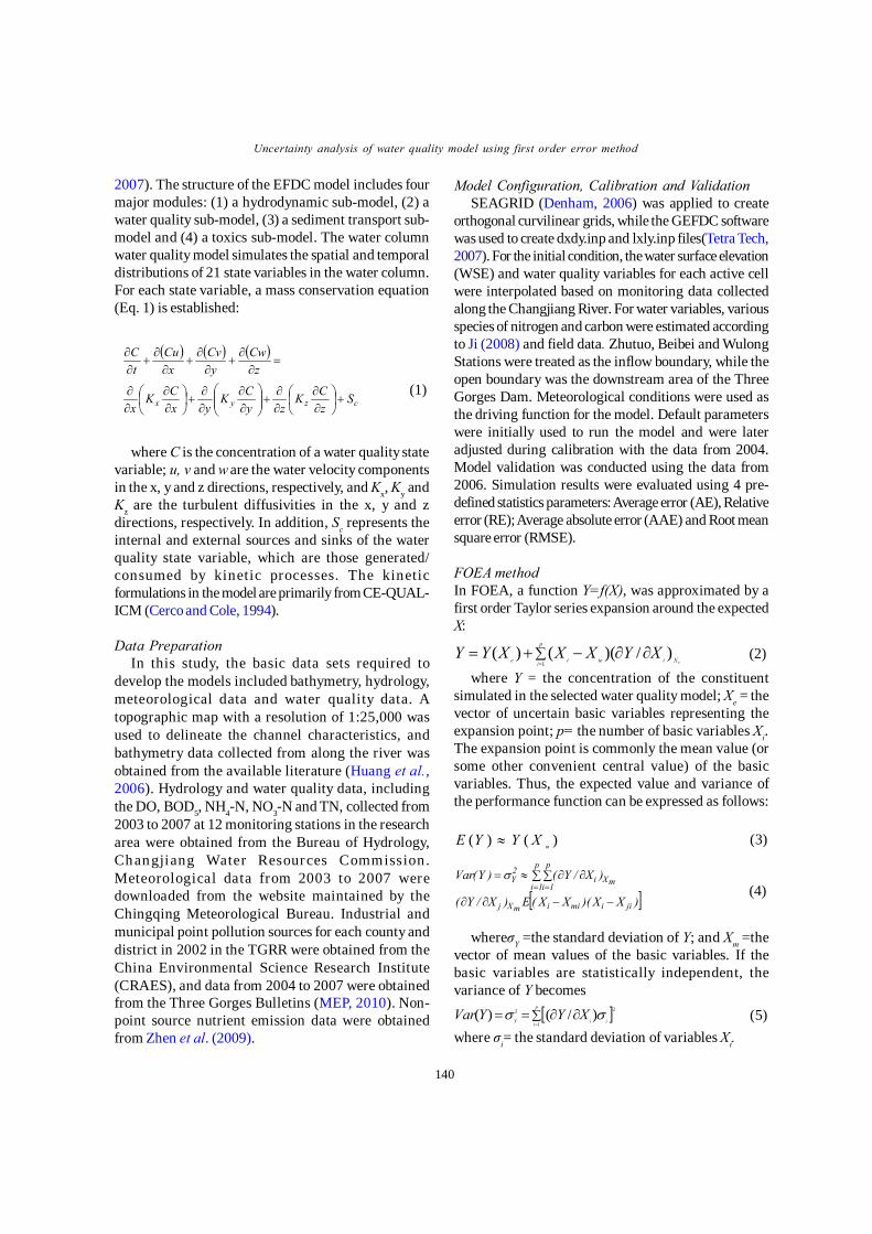
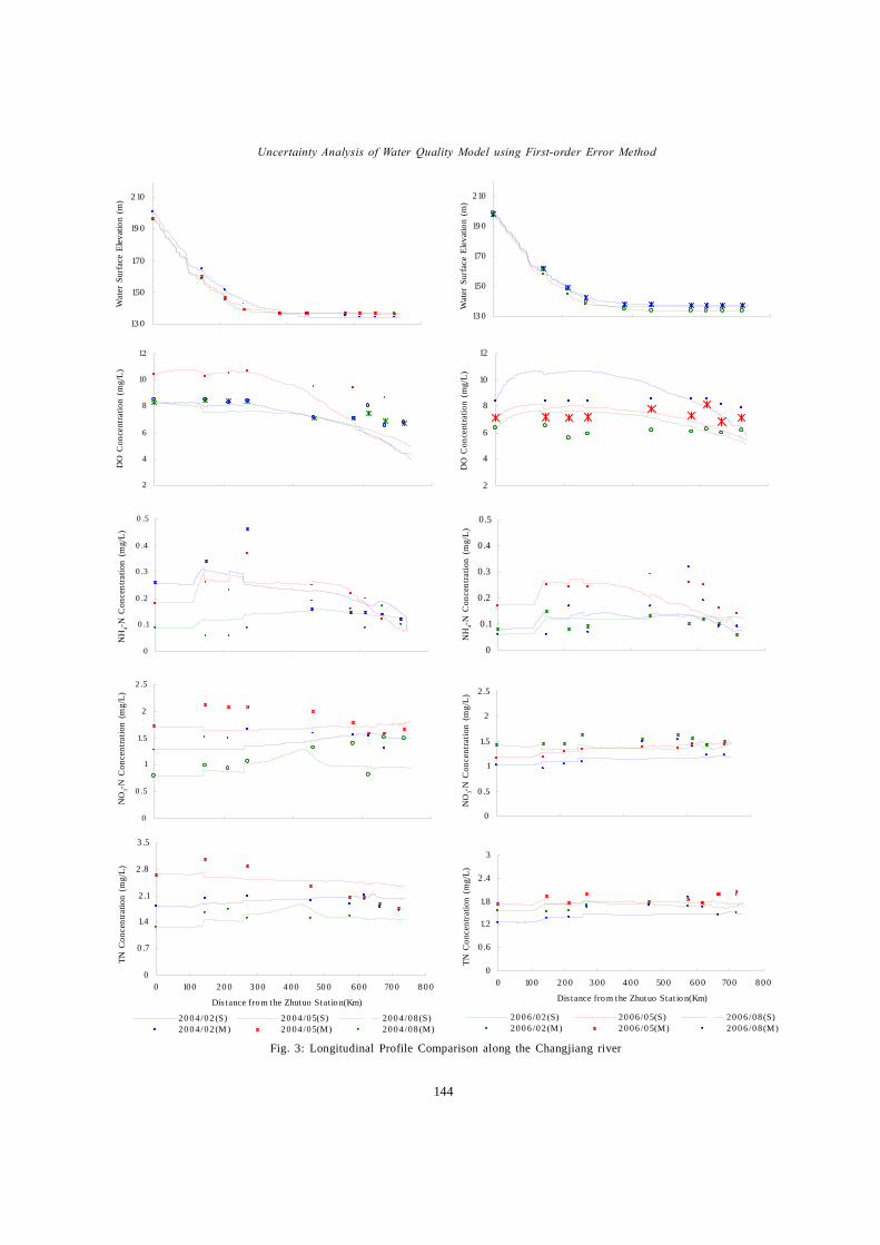
Figs. 2a’-f’ provide a comparison of the resultsobtained in Wanhzou during the verification period.The WSE (Fig. 2a’) and temperature (Fig. 2b’) weremodeled well by the model. Overall, the profile of theDO concentration (Fig. 2c’) matched the simulatedvalues well, despite some divergences near May, 2006.Some of the measured NH4-N concentrations werehigher than the simulated values during the first halfof 2006 (Fig. 2d’), and the same condition appearedduring the TN simulation (Fig. 2f’). There was also ahigh fit between the measured and simulated NO3-Nconcentration during 2006 (Fig. 2e’). These resultswere similar to those obtained during the calibrationprocess. Fig. 3 provides a longitudinal profilecomparison along the Changjiang River for thecalibration and verification period using field data fromnine stations. The dates were 2004-2-10, 2004-5-10,2004-8-10, 2006-2-10, 2006-5-10, and 2006-8-10. Figs3a and a’ indicate that the simulated WSE along theriver was satisfactory for the three flow periods. Thesimulated DO concentrations matched the measuredDO data in the upper section for each flow period(Figs. 3b and b’), but were lower than the measuredDO for the downstream stations near the Three GorgesDam. During the field measurement of DO, only thesurface DO concentration was measured; however,in the model, the simulated DO was the averaged valuealong the water depth (Tetra Tech, 2007). For NH4-N(Figs. 3c and c’), the simulation results in the averageflow period were better than in the other two periods.There was also a sharp increase in NH4-N from thedistance from 140 km to 160 km due to industrial and

domestic load emissions in Chongqing City. A largedecrease was observed at the location at which theJialingjiang River joins the impoundment area, andthe NH4-N level continued to decay until theChangshou District (214 km from the Zhutuo station),where an increase in NH4-N concentration appeared.However, after the merge with the Wujiang River (258km), the NH4-N decreased and remained low until theWanzhou District (458 km). Generally, the NO3-N(Fig.3d and Fig.3d’) and TN (Figs. 3e and e’) have thesame simulation efficacy, although an increase in TNoccurred at Chongqing City due to a large dischargeof NH4-N in the region (MEP, 2010). Table 1summarizes the error analyses of six modeled andobserved variables at three stations during thecalibration and verification periods, respectively. Theresults in Table 1 show that the modeling errors werelow. Taking RE as an example, during 2004, the REsvaried from 0.29 % for WSE at the Cuntan station to44.58 % for NH4-N at the same station. In addition,the REs were less than 15 % except for those of NH4-N. Similarly, the REs of NH4-N were also higher in2006, with the highest value of 24.64 % being observedat the Wanzhou station. This may have been causedby the large range of field data from less than 0.1 mg/l to greater than 0.5 mg/L, and the complexity ofsources and sinks (MEP, 2010).

Uncertainty analysisUncertainty analysis was conducted using the

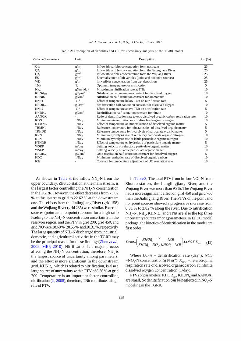
FOEA method, and three gird cells, grid 200, grid450, and grid 700, were selected to represent theupper, middle, and lower reaches. The base modelwith calibrated parameters was implemented for theentire modeling period (1 y) and changes wereconducted from upstream input, the JianglingjiangRiver input, the Wujiang River input, point andnonpoint source input, wet deposition and relatedparameters for each variable with a disturbance of5 %. The annual mean output of variables from thethree grid cells was compared with those of thebase model to calculate the normalized sensitivitycoefficient (Si), while the CV values for variablesand parameters were determined according tostudies conducted by Brown and Barnwell (1987)and Zhang and Yu (2004). Table 2 lists detailedmodel variables and parameters, units, descriptions,and CV values for uncertainty analysis using theTGRR model.

143

X. Zhao et al.Uncertainty Analysis of Water Quality Model using First-order Error Method

Fig. 3: Longitudinal Profile Comparison along the Changjiang river

144

Wat

er S

urfa

ce E

leva

tion

(m)

DO

Con

cent

ratio

n (m

g/L)

NH

4-N C

once

ntra

tion

(mg/

L)N

O3-N

Con

cent

ratio

n (m

g/L)

TN C

once

ntra

tion

(mg/

L)

13 0

150

170

19 0

2 10

0 2 0 0 4 0 0 6 0 0 8 0 0

2

4

6

8

10

12

0 2 0 0 4 0 0 6 0 0 8 0 0

0

0 .1

0 .2

0 .3

0 .4

0 .5

0 2 0 0 4 0 0 6 0 0 8 0 0

0

0 .5

1

1.5

2

2 .5

0 2 0 0 4 0 0 6 0 0 8 0 0

0

0 .7

1.4

2 .1

2 .8

3 .5

0 100 20 0 300 400 50 0 600 70 0 80 0

Dis tance from the Zhutuo Stat io n(Km)

20 0 4 /02 (S) 20 04 /05(S) 200 4 /08 (S)20 0 4 /02 (M ) 20 04 /05(M) 200 4 /08 (M)

Wat

er S

urfa

ce E

leva

tion

(m)

DO

Con

cent

ratio

n (m

g/L)

NH

4-N C

once

ntra

tion

(mg/

L)N

O3-N

Con

cent

ratio

n (m

g/L)

TN C

once

ntra

tion

(mg/

L)

13 0

150

170

19 0

2 10

0 2 00 400 6 00 8 00

2

4

6

8

10

12

0 2 0 0 4 0 0 6 0 0 8 0 0

0

0.1

0.2

0.3

0.4

0.5

0 200 400 600 800

0

0 .5

1

1.5

2

2 .5

0 20 0 40 0 600 800

0

0 .6

1.2

1.8

2 .4

3

0 100 2 00 3 00 40 0 500 60 0 70 0 8 00

Dis tance fro m the Zhutuo Stat io n(Km)

20 0 6 /02(S) 20 06 /0 5(S) 20 0 6 /08(S)20 0 6 /02(M) 20 06 /0 5(M) 20 0 6 /08(M)

X. Zhao et al.Int. J. Environ. Sci. Tech., 8 (1), 137-148, Winter 2011

Table 2: Description of variables and CV for uncertainty analysis of the TGRR model

Variable/Parameters Unit Description CV (%)

Q1i g/m3 Inflow ith varibles concentration form upstream 25 Q2i g/m3 Inflow ith varibles concentration form the Jialingjiang River 25 Q3i g/m3 Inflow ith varibles concentration form the Wujiang River 25 ES g/m3 External source of ith varibles (point and nonpoint sources) 25 WD g/m3 ith varibles concentration from wet deposition 25 TNit ℃ Optimum temperature for nitrification 5 Nitm gNm-3/day Mmaximum nitrification rate at TNit 10 KHNitDO gO2/m3 Nitrification half-saturation constant for dissolved oxygen 10 KHNitN gN/m3 Nitrification half-saturation constant for ammonium 10 KNit1 ℃-2 Effect of temperature below TNit on nitrification rate 5 KRORDO g O/m3 denitrification half-saturation constant for dissolved oxygen 10 KNit2 ℃-2 Effect of temperature above TNit on nitrification rate 5 KHDNN gN/m3 Denitrification half-saturation constant for nitrate 10 AANOX - Ratio of denitrification rate to oxic dissolved organic carbon respiration rate 10 KDN 1/Day Minimum mineralization rate of dissolved organic nitrogen 10 KTMNL 1/Day  Effect of temperature on mineralization of dissolved organic matter 5 TRMNL 1/Day  Reference temperature for mineralization of dissolved organic matter 5 TRHDR 1/Day  Reference temperature for hydrolysis of particulate organic matter 5 KRN 1/Day Minimum hydrolysis rate of refractory particulate organic nitrogen 10 KLN 1/Day Minimum hydrolysis rate of labile particulate organic nitrogen 10 KTHDR 1/Day Effect of temperature on hydrolysis of particulate organic matter 5 WSRP m/day Settling velocity of refractory particulate organic matter 10 WSLP m/day Settling velocity of labile particulate organic matter 10 KHORDO gO2/m3 Oxic respiration half-saturation constant for dissolved oxygen 5 KDC 1/Day Minimum respiration rate of dissolved organic carbon 10 KTr - Constant for temperature adjustment of DO reaeration rate. 10  

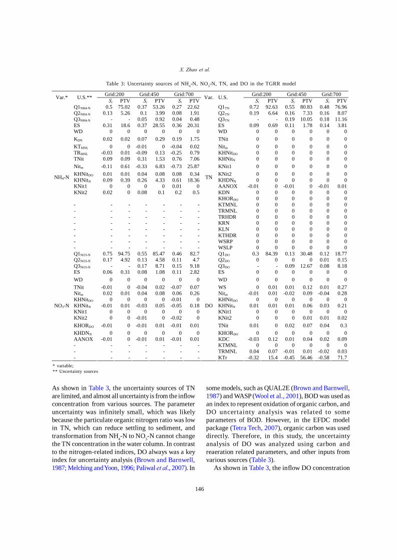
As shown in Table 3, the inflow NN4-N from theupper boundary, Zhutuo station at the main stream, isthe largest factor controlling the NH4-N concentrationin the TGRR. However, the effect decreases from 75.02% at the upstream grid to 22.62 % at the downstreamone. The effects from the Jialingjiang River (grid 158)and the Wujiang River (grid 285) were similar. Externalsources (point and nonpoint) account for a high ratioleading to the NH4-N concentration uncertainty in thereservoir region, and the PTV in grid 200, grid 450, andgrid 700 were 18.60 %, 28.55 %, and 20.31 %, respectively.The large quantity of NH4-N discharged from industrial,domestic, and agricultural activities in the TGRR maybe the principal reason for these findings(Zhen et al.,2009; MEP, 2010). Nitrification is a major processaffecting the NH4-N concentration; therefore, Nitm isthe largest source of uncertainty among parameters,and the effect is more significant in the downstreamgrid. KHNitN, which is related to nitrification, is also alarge source of uncertainty with a PTV of 8.36 % at grid700. Temperature is an important factor controllingnitrification (Ji, 2008); therefore, TNit contributes a highrate of PTV.

In Table 3, The total PTV from inflow NO3-N fromZhutuo station, the Jianglingjiang River, and theWujiang River was more than 95 %. The Wujiang Riverhad a more significant effect on gird 450 and grid 700than the Jialingjiang River. The PTVs of the point andnonpoint sources showed a progressive increase from0.31 % to 2.82 % along the river. Due to nitrificationNH4-N, Nitm, KHNitN, and TNit are also the top threeuncertainty sources among parameters. In EFDC modelpackage, the kinetics of denitrification in the model arefirst order:

DOC

NDO

DO KAANOXNOKHDN

NODOKHOR

KHORDenit ⋅⎟⎟⎠

⎞⎜⎜⎝

⎛+⎟⎟

⎠

⎞⎜⎜⎝

⎛+

=3

3 (12)

Where Denit = denitrification rate (day-1); NO3=NO3-N concentration(g N m-3); KDOC =heterotrophicrespiration rate of dissolved organic carbon at infinitedissolved oxygen concentration (1/day).

PTVs of parameters, KHORDO, KHDNN and AANOX,are small, So denitrification can be neglected in NO3-Nmodeling in the TGRR.

145

X. Zhao et al.

Table 3: Uncertainty sources of NH4-N, NO3-N, TN, and DO in the TGRR model

Grid:200 Grid:450 Grid:700 Grid:200 Grid:450 Grid:700 Var.* U.S.** Si PTV Si PTV Si PTV Var. U.S. Si PTV Si PTV Si PTVQ1NH4-N 0.5 75.02 0.37 53.26 0.27 22.62 Q1TN 0.72 92.63 0.55 80.83 0.48 76.96Q2NH4-N 0.13 5.26 0.1 3.99 0.08 1.91 Q2TN 0.19 6.64 0.16 7.33 0.16 8.07Q3NH4-N - - 0.05 0.92 0.04 0.48 Q3TN - - 0.19 10.05 0.18 11.16ES 0.31 18.6 0.37 28.55 0.36 20.31 ES 0.09 0.69 0.11 1.78 0.14 3.81WD 0 0 0 0 0 0 WD 0 0 0 0 0 0KDN 0.02 0.02 0.07 0.29 0.19 1.75 TNit 0 0 0 0 0 0KTMNL 0 0 -0.01 0 -0.04 0.02 Nitm 0 0 0 0 0 0TRMNL -0.03 0.01 -0.09 0.13 -0.25 0.79 KHNitDO 0 0 0 0 0 0TNit 0.09 0.09 0.31 1.53 0.76 7.06 KHNitN 0 0 0 0 0 0Nitm -0.11 0.61 -0.33 6.83 -0.73 25.87 KNit1 0 0 0 0 0 0KHNitDO 0.01 0.01 0.04 0.08 0.08 0.34 KNit2 0 0 0 0 0 0KHNitN 0.09 0.39 0.26 4.33 0.61 18.36 KHDNN 0 0 0 0 0 0KNit1 0 0 0 0 0.01 0 AANOX -0.01 0 -0.01 0 -0.01 0.01KNit2 0.02 0 0.08 0.1 0.2 0.5 KDN 0 0 0 0 0 0 KHORDO 0 0 0 0 0 0- - - - - - - KTMNL 0 0 0 0 0 0- - - - - - - TRMNL 0 0 0 0 0 0- - - - - - - TRHDR 0 0 0 0 0 0- - - - - - - KRN 0 0 0 0 0 0- - - - - - - KLN 0 0 0 0 0 0- - - - - - - KTHDR 0 0 0 0 0 0- - - - - - - WSRP 0 0 0 0 0 0

NH4-N

- - - - - - -

TN

WSLP 0 0 0 0 0 0Q1NO3-N 0.75 94.75 0.55 85.47 0.46 82.7 Q1DO 0.3 84.39 0.13 30.48 0.12 18.77Q2NO3-N 0.17 4.92 0.13 4.58 0.11 4.7 Q2DO 0 0 0 0 0.01 0.15Q3NO3-N - - 0.17 8.71 0.15 9.18 Q3DO - - 0.09 12.67 0.08 8.18ES 0.06 0.31 0.08 1.08 0.11 2.82 ES 0 0 0 0 0 0WD 0 0 0 0 0 0 WD 0 0 0 0 0 0TNit -0.01 0 -0.04 0.02 -0.07 0.07 WS 0 0.01 0.01 0.12 0.01 0.27Nitm 0.02 0.01 0.04 0.08 0.06 0.26 Nitm -0.01 0.01 -0.02 0.09 -0.04 0.28KHNitDO 0 0 0 0 -0.01 0 KHNitDO 0 0 0 0 0 0KHNitN -0.01 0.01 -0.03 0.05 -0.05 0.18 KHNitN 0.01 0.01 0.01 0.06 0.03 0.21KNit1 0 0 0 0 0 0 KNit1 0 0 0 0 0 0KNit2 0 0 -0.01 0 -0.02 0 KNit2 0 0 0 0.01 0.01 0.02KHORDO -0.01 0 -0.01 0.01 -0.01 0.01 TNit 0.01 0 0.02 0.07 0.04 0.3KHDNN 0 0 0 0 0 0 KHORDO 0 0 0 0 0 0AANOX -0.01 0 -0.01 0.01 -0.01 0.01 KDC -0.03 0.12 0.01 0.04 0.02 0.09- - - - - - - KTMNL 0 0 0 0 0 0- - - - - - - TRMNL 0.04 0.07 -0.01 0.01 -0.02 0.03

NO3-N

- - - - - - -

DO

KTr -0.32 15.4 -0.45 56.46 -0.58 71.7 

As shown in Table 3, the uncertainty sources of TNare limited, and almost all uncertainty is from the inflowconcentration from various sources. The parameteruncertainty was infinitely small, which was likelybecause the particulate organic nitrogen ratio was lowin TN, which can reduce settling to sediment, andtransformation from NH4-N to NO3-N cannot changethe TN concentration in the water column. In contrastto the nitrogen-related indices, DO always was a keyindex for uncertainty analysis (Brown and Barnwell,1987; Melching and Yoon, 1996; Paliwal et al., 2007). In

some models, such as QUAL2E (Brown and Barnwell,1987) and WASP (Wool et al., 2001), BOD was used asan index to represent oxidation of organic carbon, andDO uncertainty analysis was related to someparameters of BOD. However, in the EFDC modelpackage (Tetra Tech, 2007), organic carbon was useddirectly. Therefore, in this study, the uncertaintyanalysis of DO was analyzed using carbon andreaeration related parameters, and other inputs fromvarious sources (Table 3).

As shown in Table 3, the inflow DO concentration

* variable;** Uncertainty sources

146

X. Zhao et al.Int. J. Environ. Sci. Tech., 8 (1), 137-148, Winter 2011

from the Zhutuo station was dominant at grid 200 witha PTV of 84.39 %, but the effect decreased rapidly alongthe Changjiang River, with the PTV being 18.77 % atgrid 700. The uncertainty from the Jialingjiang Riverwas also small, and lower than that of the WujiangRiver. In the downstream reaches, reaeration becomesthe largest source of uncertainty for DO, and PTVs ofKTr increased significantly from 15.40 % at grid 200 to71.70 % at grid 700. Water temperature is a primaryfactor leading to larger DO concentration uncertainty,which can be reflected by TNit indirectly. Thesefindings are comparable to those of Brown andBarnwell (1987) and Abrishamchi et al. (2005) byQUAL2E. Nitrification and oxidation of organic carbonalso contributed somewhat to DO uncertainty (e.g. PTVof Nitm is 0.28 % at the grid 700).

CONCLUSIONIn this study, the input and parameter uncertainty

analysis was conducted using the FOEA method for somewater quality variables in a water quality model. DO was ageneral variable in various uncertainty analyses, but NH4-N, NO3-N, and TN were scarce. Uncertainty analysis staticwater quality models were more common than dynamicones. When compared to previously developed waterquality models, the Three Gorges Model was superior inthe following aspects: (1) it employed adequate and newerfield data, which presents water quality conditions afterimpoundment; (2) it had long calibration and verificationperiods (lasting 1 y), which enabled it to better reflect thewater quality of the TGR during low, average and highflow periods; (3) it considered more complex biochemicalprocesses. The calibration and the verification resultsrevealed that the model developed here can simulate thetransport and fate of each variable satisfactorily with smallerrors. The results of the hydrodynamics were best andthe RE values were less than 1 %. Based on the calibratedmodel, input and parameter uncertainty analysis wereconducted systematically for NH4-N, NO3-N, TN, and DOat three grid cells located in the upper, middle anddownstream portions of the research area. Based on theresults of this study, the following conclusions can bedrawn: (a) for nitrogen related variables, inflow fromupstream, two tributaries and external sources were themain sources of uncertainty; (2) for NH4-N and NO3-N,nitrification related parameters also contributed to theuncertainty; (3) for DO, reaeration is a key source ofuncertainty, especially at middle and downstreamreaches.

ACKNOWLEDGEMENTSMany thanks are given to Mr. Paul M. Craig at

Dynamic Solution LLC. for providing the full versionEFDC Explorer software and his guidance. This studywas supported by the National Natural ScienceFoundation of China (NO. 40771193) and Program forChangjiang Scholars and Innovative Research Teamin University (No.IRT0809).

REFERENCESAbrishamchi, A.; Tajrishi, M.; Shafieian, P., (2005).

Uncertainty analysis in QUAL2E model of Zayandeh-RoodRiver. Water Environ. Res., 77 (3), 279-286 (8 pages).

Bobba, A. G.; Singh, V. P.; Bengtsson, L., (1996). Applicationof First-Order and Monte Carlo analysis in watershed waterquality models. Water Res. Manage., 10 (3), 219-240 (22pages) .

Brown, L. C.; Barnwell, T. O., (1987). The enhanced streamwater quality models QUAL2E and QUAL2E-UNCAS:Documentation and user manual. US EPA, Athens, Georgia,USA.

Cerco, C. F.; Cole, T. M., (1994). Three-dimensionaleutrophication model of Chesapeake Bay: Volume1, mainreport. US Army Engineer Waterways Experiment Station,Vicksburg, Mississippi, USA.

Chapra, S.; Pelletier, G.; Tao, H., (2007). QUAL2K: A modelingframework for simulating river and stream water quality,version 2.07: documentation and users manual. Civil andEnviron. Eng. Dept., Tufts University, Medford,Massachusetts, USA.

Chen, H. W.; Yu, R. F.; Liaw, S. L.; Huang, W. C., (2010). Informationpolicy and management framework for environmental protectionorganization with ecosystem conception. Int. J. Environ.Sci. Tech., 7 (2), 313-326 (14 pages).

Deng, C. G., (2007). The study of eutrophication in the threegorges reservoir region. Chinese Environment Press, Beijing.

Denham, C. R., (2006). SeaGrid orthogonal grid maker formatlab.

DHI, (2003). MIKE 11: A modelling system for rivers andchannels:short introduction tutorial. DHI Software,Hørsholm, Denmark.

EPA, (2009). Total maximum daily loads for the NimishillenCreek watershed. OhioEPA, Columbus, Ohio, USA.

Franceschini, S.; Tsai, C. W., (2010). Assessment of uncertaintysources in water quality modeling in the Niagara River. Adv.Water Res., 33 (4), 493-503 (11 pages).

Huang, Z. L.; Li, Y. L.; Chen, Y. C.; Li, J. X.; Xing, Z. G.,(2006). Water quality prediction and water environmentalcarrying capacity calculation for Three Gorges Reservoir.China Waterpower Publisher, Beijing.

Igbinosa, E. O.; Okoh, A. I ., (2009). Impact of dischargewastewater effluents on the physico-chemical qualities of areceiving watershed in a typical rural community. Int. J.Environ. Sci. Tech., 6 (2), 175-182 (8 ages).

Igwe, J. C.; Abia, A. A.; Ibeh, C. A., (2008). Adsorption kineticsand intraparticulate diffusivities of Hg, As and Pb ions onunmodified and thiolated coconut fiber. Int. J. Environ. Sci.Tech., 5 (1), 83-92 (10 pages).

Ji, Z. G., (2008). Hydrodynamics and water quality: Modeling

147

X. Zhao et al.Uncertainty Analysis of Water Quality Model using First-order Error Method

rivers, lakes and estuaries. Wiley-Interscience, Hoboken,New Jersey.

Karim, M. R.; Sekine, M.; Ukita, M., (2002). Simulation ofeutrophication and associated occurrence of hypoxic andanoxic condition in a coastal bay in Japan. Mar. Pollut.Bull., 45 (1-12), 280-285 (6 pages).

Kuok, K. K.; Harun, S.; Shamsuddin, S. M., (2010). Particleswarm optimization feedforward neural network for modelingrunoff. Int. J. Environ. Sci. Tech., 7 (1), 67-78 (12 pages).

Li, J . X.; Liao, W. G.; Huang, Z. L., (2002). Numericalsimulation of water quality for the Three Gorges ProjectReservoir. Shuili Xuebao(China), 12, 7-10 (4 pages).

Melching, C. S.; Yoon, C. G., (1996). Key sources ofuncertainty in QUAL2E model of Passaic River. J. WaterRes. Plan. Manage., 122 (2), 105–113 (9 pages).

MEP, (2010). Three Gorges Bulletin. Ministry ofEnvironmental Protection, Beijing, China.

Nagheeby, M.; Kolahdoozan, M., (2010). Numerical modelingof two-phase fluid flow and oil slick transport in estuarinewater. Int. J. Environ. Sci. Tech., 7 (4), 771-784 (14 pages).

Paliwal, R.; Sharma, P.; Kansal, A., (2007). Water qualitymodelling of the river Yamuna (India) using QUAL2E-UNCAS. J. Environ. Manage., 83 (2), 131-144 (14 pages).

Radwan, M.; Willems, P.; Berlamont, J., (2004). Sensitivityand uncerta inty analysis for river quality modeling. J.Hydroinform., 6 (2), 83-99 (17 pages).

Ratto, M.; Saltelli, A., (2001). GLUEWIN user manual, inmodel assessment in integrated procedures for environmentalimpact evaluation: Software prototypes. Joint ResearchCentre of European Commission, Institute for the Protectionand Security of the Citizen., Ispra, Italy.

Shah, B. A.; Shah, A. V.; Singh, R. R., (2009). Sorption isothermsand kinetics of chromium uptake from wastewater usingnatural sorbent material. Int. J. Environ. Sci. Tech., 6 (1),83-92 (14 pages).

Soner Kara, S.; Onut, S., (2010). A stochastic optimizationapproach for paper recycling reverse logistics network

design under uncertainty. Int. J. Environ. Sci. Tech., 7(4), 67-78 (14 pages) .

Tetra Tech, I ., (2007). Theenvironmental flu id dynamicscode user manual US EPA Version 1 .01. Tetr a Tech,Inc., Fairfax,Virginia ,USA.

Tomassin i, L .; Reichert, P., (2 007 ). Robust Bayesianuncerta inty analysis of climate system properties usingMarkov Chain Monte Carlo methods. J. Climate, 20 (7),1239-1254 (16 pages) .

Turner, D., F. ;Pelletier, G. J.; Kasper, B., (2009). DissolvedOxygen and pH Modeling of a Periphyton Dominated,Nutrient Enriched River. J. Environ. Eng., 135 (8), 645-652 (8 pages) .

USEPA, (1999). Protocol for developing nutrient TMDLsfirst edition. USEPA, Washington,D.C. USA.

Wool, T.A.; Ambrose, R. B.;Martin, J. L.; Comer, E. A.,(2001). Water quality analysis simulation program(WASP) version 6 .0 draft: user ’ s manual. USEnvironmental Protection Agency-Region 4 , Atlanta ,USA.

Yu, X. Z., (2008). Simulation study on the effect of sedimenton phosphorus on the Three Gorges Reservoir.Ph.D.dissertation, Shool of Environment, Beijing NormalUniversity.

Zhang, H. X.; Yu, S. L., (2004). Applying the First-OrderError analysis in determining the margin of safety fortotal maximum daily load computations. J. Environ. Eng.ASCE, 130 (6), 664-673 (10 pages) .

Zhang, J . X.; Liu , Z. J .; Sun, X. X., (2009). Changinglandscape in the Three Gorges Reservoir Area of YangtzeRiver from 1977 to 2005: Land use/land cover, vegetationcover changes estimated using multi-source satellite data.Int. J. Appl. Earth Obs., 11 (6), 403-412 (10 pages) .

Zhen, B. H.; Wang, L. J.; B., G., (2009). Load of non-pointsource pollutants from upstream rivers into Three GorgesReservoir. Res. Environ., 22 (2), 125-131 (7 pages) .

How to cite this article: (Harvard style)Zhao, X.; Shen, Z. Y.; Xiong, M.; Qi, J., (2011). Key uncertainty sources analysis of water quality model using the first order errormethod. Int. J. Environ. Sci. Tech., 8 (1), 137-148.

AUTHOR (S) BIOSKETCHESZhao, X., Ph.D. Scholar, State Key Laboratory of Water Environment Simulation, School of Environment, Beijing Normal University,Beijing 100875, P. R. China. Email: zhaoxin@mail.bnu.edu.cn

Shen, Z. Y., Ph.D., Full Professor, State Key Laboratory of Water Environment Simulation, School of Environment, Beijing NormalUniversity, Beijing 100875, P. R. China. Email: zyshen@bnu.edu.cn

Xiong, M., Ph.D., Bureau of Hydrology, Changjiang Water Resources Commission, Wuhan, Hubei Province 430010, P. R. China. Email:Xiongming@cjh.com.cn

Qi, J., Ph.D., Beijing Municipal Research Institute of Environmental Protection, Beijing 100037, P. R. China. Email: qijun@foxmail.com

148