kernel smoothing methods (part 1) - georgetown...

Kernel Smoothing Methods (Part 1)

Henry Tan

Georgetown University

April 13, 2015

Georgetown University Kernel Smoothing 1

Introduction - Kernel Smoothing

Previously

Basis expansions and splines.

Use all the data to minimise least squares of a piecewise definedfunction with smoothness constraints.

Kernel Smoothing

A different way to do regression.

Not the same inner product kernel we’ve seen previously


Kernel Smoothing

In Brief

For any query point x0, the value of the function at that point f (x0) issome combination of the (nearby) observations, s.t., f (x) is smooth.

The contribution of each observation xi , f (xi ) to f (x0) is calculated usinga weighting function or Kernel Kλ(x0, xi ).

λ - the width of the neighborhood


Kernel Introduction - Question

Question

Sicong 1) Comparing Equa. (6.2) and Equa. (6.1), it is using the Kernelvalues as weights on yi to calculate the average. What could be theunderlying reason for using Kernel values as weights?

Answer

By definition, the kernel is the weighting function.The goal is to give more importance to closer observations withoutignoring observations that are further away.


K-Nearest-Neighbor Average

Consider a problem in 1 dimension x-A simple estimate of f (x0) at any point x0 is the mean of the k pointsclosest to x0.

f (x) = Ave(yi |xi ∈ Nk(x)) (6.1)


KNN Average Example

True functionKNN averageObservations contributing to f (x0)


Problem with KNN Average

Problem

Regression function f (x) is discontinuous - “bumpy”.Neighborhood set changes discontinuously.

Solution

Weigh all points such that their contribution drop off smoothly withdistance.


Epanechnikov Quadratic Kernel Example

Estimated function is smoothYellow area indicates the weight assigned to observations in that region.


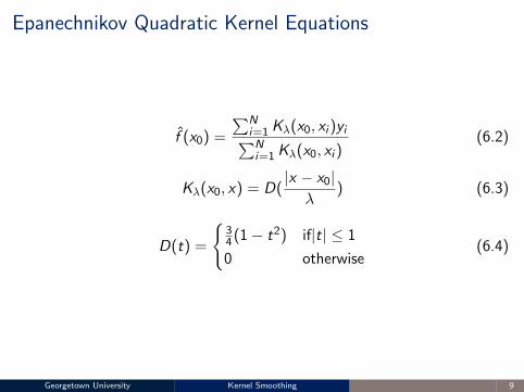
Epanechnikov Quadratic Kernel Equations

f (x0) =

∑Ni=1 Kλ(x0, xi )yi∑Ni=1 Kλ(x0, xi )

(6.2)

Kλ(x0, x) = D(|x − x0|

λ) (6.3)

D(t) =

{34(1− t2) if|t| ≤ 1

0 otherwise(6.4)


KNN vs Smooth Kernel Comparison


Other Details

Selection of λ - covered later

Metric window widths vs KNN widths - bias vs variance

Nearest Neigbors - multiple observations with same xi - replace withsingle observation with average yi and increase weight of thatobservation

Boundary problems - less data at the boundaries (covered soon)


Popular Kernels

Epanechnikov Compact (only local observations have non-zero weight)

Tri-cube Compact and differentiable at boundary

Gaussian density Non-compact (all observations have non-zero weight)


Popular Kernels - Question

Question

Sicong2) The presentation in Figure. 6.2 is pretty interesting, it mentions that“The tri-cube kernel is compact and has two continuous derivatives at theboundary of its support, while the Epanechnikov kernel has none.” Canyou explain this more in detail in class?

Answer

Tricube Kernel - D(t) =

{(1− |t|3)3 if|t| ≤ 1;

0 otherwise

D ′(t) = 3 ∗ (−3t2)(1− |t|3)2

Epanechnikov Kernel - D(t) =

{34 (1− t2) if|t| ≤ 1;

0 otherwise


Problems with the Smooth Weighted Average

Boundary Bias

At some x0 at a boundary, more of the observations are on one side of the x0 -The estimated value becomes biased (by those observations).


Local Linear Regression

Constant vs Linear Regression

Technique described previously : equivalent to local constant regression ateach query point.Local Linear Regression : Fit a line at each query point instead.

Note

The bias problem can exist at an internal query point x0 as well if theobservations local to x0 are not well distributed.


Local Linear Regression


Local Linear Regression Equations

minα(x0),β(x0)

N∑i=1

Kλ(x0, x1)[yi − α(x0)− β(x0)xi ]2 (6.7)

Solve a separate weighted least squares problem at each target point (i.e.,solve the linear regression on a subset of weighted points).

Obtain f (x0) = α(x0) + β(x0)x0where α, β are the constants of the solution above for the query point x0


Local Linear Regression Equations 2

f (x0) = b(x0)T (BTW(x0)B)−1BTW(x0)y (6.8)

=N∑i=1

li (x0)yi (6.9)

6.8 : General solution to weighted local linear regression6.9 : Just to highlight that this is a linear model (linear contribution fromeach observation).


Question - Local Linear Regression Matrix

Question

Yifang1. What is the regression matrix in Equation 6.8? How does not Equation6.9 derive from 6.8?

Answer

Apparently, for a linear model (i.e., the solution is comprised of a linearsum of observations), the least squares minimization problem has thesolution as given by Equation 6.8.Equation 6.9 can be obtained from 6.8 by expansion, but it isstraightforward since y only shows up once.


Historical (worse) Way of Correcting Kernel Bias

Modifying the kernel based on “theoretical asymptotic mean-square-errorconsiderations” (don’t know what this means, probably not important).

Linear local regression : Kernel correction to first order (automatic kernelcarpentry)


Locally Weighted Regression vs Linear Regression -Question

Question

Grace 2. Compare locally weighted regression and linear regression that welearned last time. How does the former automatically correct the modelbias?

Answer

Interestingly, simply by solving a linear regression using local weights, thebias is accounted for (since most functions are approximately linear at theboundaries).


Local Linear Equivalent Kernel

Dots are the equivalent kernel weight li (x0) from 6.9Much more weight are given to boundary points.


Bias Equation

Using a taylor series expansion on f (x0) =N∑i=1

li (x0)f (xi ),

the bias f (x0)− f (x0) is dependent only on superlinear terms.

More generally, polynomial-p regression removes the bias of p-order terms.


Local Polynomial Regression

Local Polynomial Regression

Similar technique - solve the least squares problem for a polynomialfunction.

Trimming the hills and Filling the valleys

Local linear regression tends to flatten regions of curvature.


Question - Local Polynomial Regression

Question

Brendan 1) Could you use a polynomial fitting function with an asymptoteto fix the boundary variance problem described in 6.1.2?

Answer

Ask for elaboration in class.


Question - Local Polynomial Regression

Question

Sicong 3) In local polynomial regression, can the parameter d also be avariable rather than a fixed value? As in Equa. (6.11).

Answer

I don’t think so. It seems that you have to choose the degree of yourpolynomial before you can start solving the least squares minimizationproblem.


Local Polynomial Regression - Interior Curvature Bias


Cost to Polynomial Regression

Variance for Bias

Quadratic regression reduces the bias by allowing for curvature.Higher order regression also increases variance of the estimated function.


Variance Comparisons


Final Details on Polynomial Regression

Local linear removes bias dramatically at boundaries

Local quadratic increases variance at boundaries but doesn’t helpmuch with bias.

Local quadratic removes interior bias at regions of curvature

Asymptotically, local polynomials of odd degree dominate localpolynomials of even degree.


Kernel Width λ

Each kernel function Kλ has a parameter which controls the size of thelocal neighborhood.

Epanechnikov/Tri-cube Kernel , λ is the fixed size radius around thetarget point

Gaussian kernel, λ is the standard deviation of the gaussian function

λ = k for KNN kernels.


Kernel Width - Bias Variance Tradeoff

Small λ = Narrow Window

Fewer observations, each contribution is closer to x0:High variance (estimated function will vary a lot.)Low bias - fewer points to bias function

Large λ = Wide Window

More observations over a larger area:Low variance - averaging makes the function smootherHigher bias - observations from further away contribute to the value at x0


Local Regression in Rp

Previously, we considered problems in 1 dimension.Local linear regression fits a local hyperplane, by weighted least squares,with weights from a p-dimensional kernel.

Example : dimensions p = 2, polynomial degree d = 2

b(X ) = (1,X1,X2,X21 ,X

22 ,X1X2)

At each query point x0 ∈ Rp, solve

minβ(x0)

N∑i=1

Kλ(x0, x1)(yi − b(xi )Tβ(x0))2

to obtain fit f (x0) = b(x0)T β(x0)


Kernels in Rp

Radius based Kernels

Convert distance based kernel to radius based: D( x−x0λ )→ D( ||x−x0||λ )

The Euclidean norm depends on the units in each coordinate - eachpredictor variable has to be normalised somehow, e.g., unit standarddeviation, to weigh them properly.


Question - Local Regression in Rp

Question

YifangWhat is the meaning of “local” in local regression? Equation 6.12 uses akernel mixing polynomial kernel and radial kernel?

Answer

I think “local” still means weighing observations based on distance fromthe query point.


Problems with Local Regression in Rp

Boundary problem

More and more points can be found on the boundary as p increases.Local polynomial regression still helps automatically deal with boundaryissues for any p

Curse of Dimensionality

However, for high dimensions p > 3, local regression still isn’t very useful -As with the problem with Kernel width,

difficult to maintain localness of observations (for low bias)

sufficient samples (for low variance)

Since the number of samples increases exponentially in p.

Non-visualizable

Goal of getting a smooth fitting function is to visualise the data which isdifficult in high dimensions.


Structured Local Regression Models in Rp

Structured Kernels

Use a positive semidefinite matrix A to weigh the coordinates (instead ofnormalising all of them) -

Kλ,A(x0, x) = D( (x−x0)TA(x−x0)λ )

Simplest form is the diagonal matrix which simply weighs the coordinateswithout considering correlations.General forms of A are cumbersome.


Question - ANOVA Decomposition and Backfitting

Question

Brendan 2. Can you touch a bit on the backfitting described in 6.4.2? Idon’t understand the equation they give for estimating gk .


Structured Local Regression Models in Rp - 2

Structured Regression Functions

Ignore high order correlations, perform iterative backfitting on eachsub-function.

In more detail

Analysis-of-variance (ANOVA) decomposition form-

f (X1,X2, ...,Xp) = α +∑jgj(Xj) +

∑k<l

gkl(Xk ,Xl) + ...

Ignore high order cross terms, e.g., gklm(Xk ,Xl ,Xm) (to reduce complexity)

Iterative backfitting -Assume that all terms are known except for some gk(Xk).Perform local (polynomial) regression to find gk(Xk).Repeat for all terms, and repeat until convergence.


Structured Local Regression Models in Rp - 3

Varying Coefficients Model

Perform regression over some variables while keeping others constant.

Select the first p out of q predictor variables from (X1,X2, ...,Xq) andexpress the function asf (X ) = α(Z ) + β1(Z )X1 + ...+ βq(Z )Xq

where for any given z0, the coefficients α, βi are fixed.

This can be solved using the same locally weighted least squares problem.


Varying Coefficients Model Example

Human Aorta Example

Predictors - (age, gender, depth) , Response - diameterLet Z be (gender, depth) and model diameter as a function of depth


Question - Local Regression vs Structured Local Regression

Question

Tavish1. What is the difference between Local Regression and Structured LocalRegression? And is there any similarity between the “structuring”described in this chapter to the one described in previous one where theinput are transformed/structured into a different inputs that are fed tolinear models?

Answer

Very similar I think. But the interesting thing is that different methodshave different “natural” ways to perform the transformations orsimplifications.


Discussion Question

Question

Tavish3)As a discussion question and also to understand better, this main idea ofthis chapter to find the best parameters for kernels keeping in mind thevariance-bias tradeoff. I would like to know more as to how a goodfit/model can be achieved and what are the considerations for trading offvariance for bias and vice-versa? It would be great if we can discuss someexamples.

Starter Answer

As far as the book goes - if you want to examine the boundaries, use alinear fit for reduced bias. If you care more abount interior points, use aquadratic fit to reduce internal bias (without as much of a cost in internalvariance).


kernel smoothing methods (part 1) - georgetown...

Documents