kernel ridge vs. principal component regression: minimax ...djhsu/papers/kernel-reg-ejs.pdfkernel...

Electronic Journal of StatisticsVol. 11 (2017) 1022–1047ISSN: 1935-7524DOI: 10.1214/17-EJS1258

Kernel ridge vs. principal component

regression: Minimax bounds and the

qualification of regularization operators

Lee H. Dicker

Department of Statistics and BiostatisticsRutgers UniversityPiscataway, NJ

e-mail: [email protected]

Dean P. Foster

Amazon Inc.New York, NY

e-mail: [email protected]

and

Daniel Hsu

Department of Computer ScienceColumbia University

New York, NYe-mail: [email protected]

Abstract: Regularization is an essential element of virtually all kernelmethods for nonparametric regression problems. A critical factor in theeffectiveness of a given kernel method is the type of regularization thatis employed. This article compares and contrasts members from a generalclass of regularization techniques, which notably includes ridge regressionand principal component regression. We derive an explicit finite-sample riskbound for regularization-based estimators that simultaneously accounts for(i) the structure of the ambient function space, (ii) the regularity of thetrue regression function, and (iii) the adaptability (or qualification) of theregularization. A simple consequence of this upper bound is that the riskof the regularization-based estimators matches the minimax rate in a vari-ety of settings. The general bound also illustrates how some regularizationtechniques are more adaptable than others to favorable regularity prop-erties that the true regression function may possess. This, in particular,demonstrates a striking difference between kernel ridge regression and ker-nel principal component regression. Our theoretical results are supportedby numerical experiments.

MSC 2010 subject classifications: 62G08.

∗DH acknowledges support from NSF grants DMR-1534910 and IIS-1563785 and a SloanResearch Fellowship; LHD’s work was partially supported by NSF grants DMS-1208785 andDMS-1454817.

1022

http://projecteuclid.org/ejs

http://dx.doi.org/10.1214/17-EJS1258

mailto:[email protected]



Kernel ridge vs. principal component regression 1023

Keywords and phrases: Nonparametric regression, reproducing kernelHilbert space.

Received August 2016.

1. Introduction

Suppose that the observed data consists of zi = (yi,xi), i = 1, . . . , n, whereyi ∈ Y ⊆ R and xi ∈ X ⊆ R

d. Suppose further that z1, . . . , zn ∼ ρ are iid fromsome probability distribution ρ on Y × X . Let ρ(· | x) denote the conditionaldistribution of yi given xi = x ∈ X and let ρX denote the marginal distributionof xi. Our goal is to use the available data to estimate the regression functionof y on x,

f†(x) =

∫Yy dρ(y | x) ,

which minimizes the mean-squared prediction error∫Y×X

(y − f(x)

)2dρ(y,x)

over ρX -measurable functions f : X → R. More specifically, for an estimator fdefine the risk

Rρ(f) = E

[∫ (f†(x)− f(x)

)2

dρX (x)

]= E

[‖f† − f‖2ρX

], (1)

where the expectation is computed over z1, . . . , zn, and ‖ · ‖ρX denotes the norm

on L2(ρX ); we seek estimators f which minimize Rρ(f).This is a version of the random design nonparametric regression problem.

There is a vast literature on nonparametric regression, along with a huge varietyof corresponding methods (e.g., Gyorfi et al., 2002; Wasserman, 2006). In thispaper, we focus on regularization and kernel methods for estimating f†.1 Mostof our results apply to general regularization operators. However, our motivatingexamples are two well-known regularization techniques: Kernel ridge regression(which we refer to as “KRR”; KRR is also known as Tikhonov regularization)and kernel principal component regression (“KPCR”; also known as spectralcut-off regularization).

Our main theorem is a new upper bound on the risk of a general class ofkernel-regularization methods, which includes both KRR and KPCR (Theo-rem 1). The theorem substantially generalizes previously published bounds (seeSection 2 for a discussion of related work) and illustrates the dependence of therisk on three important features: (i) the structure of the ambient reproducingkernel Hilbert space (RKHS), (ii) the specific regularization technique employed,and (iii) the regularity (often interpreted as smoothness) of the function to be

1Here, we mean “kernel” as in reproducing kernel Hilbert space, rather than kernel-smoothing, which is another popular approach to nonparametric regression.

1024 L. H. Dicker et al.

estimated. One consequence of the theorem is that the regularization methodsstudied in this paper (including KRR and KPCR) achieve the minimax rate forestimating f† in a variety of settings. A second consequence is that certain reg-ularization methods (including KPCR, but not KRR) may adapt to favorableregularity of f† to attain even faster convergence rates, while others (notablyKRR) are limited in this regard due to a well-known saturation effect (Neubauer,1997; Mathe, 2005; Bauer et al., 2007). This illustrates a striking advantage thatKPCR may have over KRR in these settings.

2. Related work

Kernel ridge regression has been studied extensively in the literature. Indeed,bounds for KRR that are similar to our Theorem 1 have been derived by Capon-netto and De Vito (2007). Moreover, it is well-known that KRR is minimax inmany of the settings considered in this paper, such as those described in Corol-laries 1–3 (Caponnetto and De Vito, 2007; Zhang, 2005; Zhang et al., 2013; Linet al., 2016). However, these cited results apply only to KRR, while the resultsin this paper apply to a substantially larger class of regularization operators(including, for example, KPCR).

Beyond KRR, there has also been significant research into more general regu-larization methods, like those considered in this paper. However, our bounds aresharper than previously published results on general regularization operators.For instance, unlike our Theorem 1, the bounds of Bauer et al. (2007) do notillustrate the dependence of the risk on the ambient Hilbert space. Thus, whileour approach immediately implies that many of the regularization methods un-der consideration are minimax optimal, it seems difficult (if not impossible) todraw this conclusion using the approach of Bauer et al. (2007). General regu-larization operators are also studied by Caponnetto and Yao (2010), but theirresults apply to semi-supervised settings where an additional pool of unlabeleddata is available.

One of the major practical implications of this paper is that KPCR mayhave significant advantages over KRR in some settings. This has been observedpreviously by other researchers; others have even noted that Tikhonov regular-ization (KRR) saturates, while spectral cut-off regularization (KPCR) does not(Mathe, 2005; Bauer et al., 2007; Lo Gerfo et al., 2008). Our results (Theorem1 and Corollaries 1–3) sharpen these observations by precisely quantifying theadvantages of unsaturated regularization operators in terms of adaptability andminimaxity. In other related work, Dhillon et al. (2013) have illustrated thepotential advantages of KPCR over KRR in finite-dimensional problems withlinear kernels; though their work is not framed in terms of saturation and generalregularization operators, it relies on similar concepts.

After the initial submission of our work, we became aware of simultaneousindependent work by Blanchard and Mucke (2016) that proves upper boundson the risk for a comparable class of regularization methods (which includesKRR and KPCR), as well as minimax lower bounds that match the upper


bounds; their results are specialized to RKHS’s where the covariance opera-tor has polynomially decaying eigenvalues. Compared to that work, our resultsrequire a weaker moment condition on the noise for risk bounds, apply to amuch broader class of RKHS’s, and also consider target functions that live infinite-dimensional subspaces (see Proposition 1). Another distinguishing featureof the present work is that it contains numerical experiments that illustrate theimplications of our theoretical bounds in some practical settings (Section 6).

Other important recent work was pointed out to us by a reviewer. Optimalrates in expectation for KRR and more general regularization methods are de-rived by Lin et al. (2016) and Guo et al. (2016), respectively, for distributedlearning problems. The bounds in the latter paper, when specialized to the non-distributed setting, are similar to those in this paper and by Blanchard andMucke (2016). However, the results in this paper are more general (for non-distributed learning), because they do not require continuity of the kernel andhave weaker conditions on the output variable.

The main engine behind the technical results in this paper is a collection oflarge-deviation results for Hilbert-Schmidt operators. The required machinery isdeveloped in the Appendices. These results build on straightforward extensionsof results of Tropp (2015). Our most precise results for KPCR and achievingparametric rates for estimation over finite-dimensional subspaces (Proposition 1)rely on slightly different arguments, which are based on well-known eigenvalueperturbation results that have been adapted to handle Hilbert-Schmidt opera-tors (e.g., the Davis-Kahan sinΘ theorem (Davis and Kahan, 1970)).

3. Statistical setting and assumptions

Our basic assumption on the distribution of z = (y,x) ∼ ρ is that the residualvariance is bounded; more specifically, we assume that there exists a constantσ2 > 0 such that ∫

Y

[y − f†(x)

]2dρ(y | x) ≤ σ2 (2)

for almost all x ∈ X . Zhang et al. (2013) also assume (2); this assumptionis slightly weaker than the analogous assumption used by Bauer et al. (2007)(equation (1) in their paper). Note that (2) holds if y is bounded almost surelyor if y = f†(x) + ε, where ε is independent of x, E(ε) = 0, and Var(ε) = σ2.

Let K : X ×X → R be a symmetric positive-definite kernel function. We as-sume thatK is bounded—i.e., that there exists κ2 > 0 such that supx∈X K(x,x)≤ κ2. Additionally, we assume that there is a countable orthonormal basis{ψj}∞j=1 ⊆ L2(ρX ) and a sequence of corresponding real numbers t21 ≥ t22 ≥· · · ≥ 0 such that

K(x, x) =

∞∑j=1

t2jψj(x)ψj(x) , x, x ∈ X , (3)

where the convergence is absolute and uniform over x, x ∈ X . Mercer’s theoremand various generalizations give conditions under which representations like (3)


are known to hold (Carmeli et al., 2006); one of the simplest examples is whenX is a compact Hausdorff space, ρX is a probability measure on the Borel setsof X , and K is continuous. Observe that

∞∑j=1

t2j =

∞∑j=1

t2j

∫Xψj(x)

2 dρX (x) =

∫XK(x,x) dρX (x) ≤ κ2 ;

in particular, {t2j} ∈ �1(N). Additionally, t2j and ψj are eigenvalues and eigen-

functions, respectively, of the linear transformation T : L2(ρX ) → L2(ρX ) de-fined by

(Tf)(x) =

∫Xf(x)K(x, x) dρX (x) =

∞∑j=1

t2j 〈f, ψj〉L2(ρX )ψj(x), (4)

for f ∈ L2(ρX ), x ∈ X , where 〈·, ·〉L2(ρX ) denotes the inner product on L2(ρX ).Let H ⊆ L2(ρX ) be the RKHS corresponding to K (Aronszajn, 1950) and let

φj = tjψj , j = 1, 2, . . .. It follows from basic facts about RKHSs that {φj}∞j=1

is an orthonormal basis for H (if t2J > t2J+1 = 0, then{φj

}J

j=1is an orthonormal

basis for H). Furthermore, H is characterized by

H =

⎧⎨⎩f =

∞∑j=1

θjψj ∈ L2(ρX );∞∑j=1

θ2jt2j

< ∞

⎫⎬⎭

and the inner product

〈f, f〉H =

⟨ ∞∑j=1

θjψj ,

∞∑j=1

θjψj

⟩H

=

∞∑j=1

θj θjt2j

(the corresponding norm is denoted by ‖ · ‖H). Our main assumption on therelationship between y, x, and the kernel K is that

f† ∈ H . (5)

This is a regularity or smoothness assumption on f†. Many of the results in thispaper can be modified, so that they apply to settings where f† /∈ H, by replacingf† with an appropriate projection of f† and including an approximation errorterm in the corresponding bounds. This approach leads to the study of oracleinequalities (Zhang, 2005; Zhang et al., 2013; Koltchinskii, 2006; Steinwart et al.,2009; Hsu et al., 2014), which we do not pursue in detail here. However, investi-gating oracle inequalities for general regularization operators may be of interestfor future research, as most existing work focuses on ridge regularization.

Another interpretation of condition (5) is that it is a minimal regularity con-dition on f† for ensuring that f† can be estimated consistently using the kernelmethods considered below. One key aspect of the upper bounds in Section 5 is


that they show f† can be estimated more efficiently, if it satisfies stronger reguar-lity conditions (and if the regularization method used is sufficiently adaptable).A convenient way to formulate a collection of regularity conditions with varyingstrengths, which will be useful in the sequel, is as follows. For ζ ≥ 0, define theHilbert space

Hζ =

⎧⎨⎩f =

∞∑j=1

θjψj ∈ L2(ρX );

∞∑j=1

θ2j

t2(1+ζ)j

< ∞

⎫⎬⎭ . (6)

Then H = H0 and Hζ2 ⊆ Hζ1 whenever ζ2 ≥ ζ1 ≥ 0. The norm on Hζ is

defined by ‖f‖2Hζ=

∑∞j=1

θ2j

t2(1+ζ)j

. Additionally, positive integers J define the

finite-rank subspace

H◦J =

⎧⎨⎩f =

J∑j=1

θjψj ∈ L2(ρX ); θ1, . . . , θJ ∈ R

⎫⎬⎭ . (7)

We have the inclusion H◦J ⊆ H◦

J+1 and, if t21, . . . , t2J > 0, then H◦

J ⊆ Hζ for

any ζ ≥ 0. In particular, it is clear from (6)–(7) that f† ∈ Hζ is a strongerregularity condition than f† ∈ H and that f† ∈ H◦

J is an even stronger condition(provided the t2j are strictly positive). Conditions such as f† ∈ Hζ and f† ∈ H◦

J

are known as source conditions elsewhere in the literature (e.g., Bauer et al.,2007; Caponnetto and Yao, 2010).

4. Regularization

As discussed in Section 1, our goal is find estimators f that minimize the risk (1).In this paper, we focus on regularization-based estimators for f†. In order to pre-cisely describe these estimators, we require some additional notation for variousoperators that will be of interest, and some basic definitions from regularizationtheory.

4.1. Finite-rank operators of interest

For x ∈ X , defineKx ∈ H byKx(x) = K(x, x), x ∈ X . LetX = (x1, . . . ,xn)� ∈

Rn×d and y = (y1, . . . , yn)

� ∈ Rn. Additionally, define the finite-rank linear

operators SX : H → Rn and TX : H → H (both depending on X) by

SXf = (〈f,Kx1〉H, . . . , 〈f,Kxn〉H)� = (f(x1), . . . , f(xn))� ,

TXf =1

n

n∑i=1

〈f,Kxi〉HKxi =1

n

n∑i=1

f(xi)Kxi , (8)

where f ∈ H. Let 〈·, ·〉Rn denote the normalized inner-product on Rn, defined

by 〈v, v〉Rn = n−1v�v for v = (v1, . . . , vn)�, v = (v1, . . . , vn)

� ∈ Rn. Then


the adjoint of SX with respect to 〈·, ·〉H and 〈·, ·〉Rn , S∗X : Rn → H, is given

by S∗Xv = 1

n

∑ni=1 viKxi . Additionally, we have TX = S∗

XSX . Finally, observethat SXS∗

X : Rn → Rn is given by the n × n matrix SXS∗

X = n−1K, whereK = (K(xi,xj))1≤i,j≤n; K is the kernel matrix, which is ubiquitous in kernelmethods and enables finite computation.

4.2. Basic definitions

A family of functions gλ : [0,∞) → [0,∞) indexed by λ > 0 is called a regular-ization family if it satisfies the following three conditions:2

R1 sup0<t≤κ2 |tgλ(t)| < 1.R2 sup0<t≤κ2 |1− tgλ(t)| ≤ 1.R3 sup0<t≤κ2 |gλ(t)| < λ−1.

The main idea behind a regularization family is that it “looks” similar to t �→1/t, but is better-behaved near t = 0, i.e., it is bounded by λ−1. An importantquantity that is related to the adaptability of a regularization family is thequalification of the regularization. The qualification of the regularization family{gλ}λ>0 is defined to be the maximal ξ ≥ 0 such that

sup0<t≤κ2

|1− tgλ(t)|tξ ≤ λξ .

If a regularization family has qualification ξ, we say that it “saturates at ξ.”Two regularization families that are the major motivation for the results in thispaper are ridge (Tikhonov) regularization, where gλ(t) = 1

t+λ , and principalcomponent (spectral cut-off) regularization, where

gλ(t) =1

t1{t ≥ λ} . (9)

Observe that ridge regularization has qualification 1 and principal componentregularization has qualification ∞. Another example of a regularization familywith qualification∞ is the Landweber iteration, which can be viewed as a specialcase of gradient descent (see, e.g., Rosasco et al., 2005; Bauer et al., 2007; LoGerfo et al., 2008).

4.3. Estimators

Given a regularization family {gλ}λ>0, we define the gλ-regularized estimatorfor f†,

fλ = gλ(TX)S∗Xy . (10)

Here, gλ is applied to the spectrum of the self-adjoint finite-rank operatorTX via the functional calculus (see, e.g., Reed and Simon, 1980, Ch. 7); this

2This definition follows Engl et al. (1996) and Bauer et al. (2007), but is slightly morerestrictive.


is a generalization of standard matrix functions (Tropp, 2015, Ch. 2). Since

S∗Xgλ(K/n) = gλ(TX)S∗

X , we have the finitely computable representation fλ =S∗Xgλ(K/n)y =

∑ni=1 γiKxi , where (γ1, . . . , γn)

� = gλ(K/n)y/n; computingthe γi involves an eigenvalue decomposition of the matrix K. The dependenceof fλ on the regularization family is implicit; our results hold for any regular-ization family except where explicitly stated otherwise. The estimators fλ arethe main focus of this paper.

5. Main results

5.1. General bound on the risk

Theorem 1. Let fλ be the estimator defined in (10) with regularization family{gλ}λ>0. Let 0 ≤ δ ≤ 1 and assume that there is some κ2

δ > 0 such that

supx∈X

∞∑j=1

t2(1−δ)j ψj(x)

2 ≤ κ2δ < ∞ (11)

Assume that the source condition f† ∈ Hζ holds for some ζ ≥ 0, and thatgλ has qualification at least max{(ζ + 1)/2, 1}. Define the effective dimension

dλ =∑∞

j=1

t2jt2j+λ

. Finally, assume that (8/3 + 2√5/3)κ2

δ/n ≤ λ1−δ ≤ κ2δ. The

following risk bound holds:

Rρ(fλ) ≤ 2ζ+3‖f†‖2Hζλζ+1 +

4dλσ2

n(12)

+ 4dλ

(‖f†‖2Ht21 +

κ2σ2

λn

)exp

(−3λ1−δn

28κ2δ

)

+ 1{ζ > 1} · 16ζ2(3/2)ζ−1 · ‖f†‖2Hζ(t21 + λ)ζ−1κ4

(34

n+

15

n2

).

Theorem 1 is proved in the Appendices. The first two terms in the upperbound (12) are typically the dominant terms. In the upper bound (12), theinteraction between the kernel K and the distribution ρX is reflected in theeffective dimension dλ (see, e.g., Zhang, 2005; Caponnetto and De Vito, 2007).The regularity of f† enters through norm of f† (both the H- and Hζ-norms)and the exponent on λ.

The condition (11) in Theorem 1 is always satisfied by taking δ = 0 and κ20 =

κ2. Requiring (11) with δ > 0 imposes additional conditions on the RKHSH. ForCorollary 1 below (which applies when the eigenvalues {t2j} have polynomial-

decay), we take δ = 0 and κ20 = κ2. The stronger condition with δ > 0 is

required to obtain obtain minimax rates for kernels where the eigenvalues {t2j}have exponential or Gaussian-type decay (see Corollaries 2–3).

Risk bounds on general regularization estimators similar to fλ were previ-ously obtained by Bauer et al. (2007). However, their bounds (e.g., Theorem


10 of Bauer et al., 2007) are independent of the ambient RKHS H, i.e., theydo not depend on the eigenvalues {t2j}. Our bounds are tighter than those ofBauer et al. because we take advantage of the structure of H. In contrast withour Theorem 1, the results of Bauer et al. do not give minimax bounds (noteasily, at least), because minimax rates must depend on the t2j .

5.2. Implications for kernels characterized by their eigenvalues’ rateof decay

We now state consequences of Theorem 1 that give explicit rates for estimatingf† via fλ, for any regularization family, under specific assumptions about thedecay rate of the eigenvalues {t2j}.

We first consider the case where the eigenvalues have polynomial decay.

Corollary 1. Assume that C ≥ 0 and ν > 1/2 are constants such that 0 <t2j ≤ Cj−2ν for all j = 1, 2, . . .. Assume the source condition f† ∈ Hζ for someζ ≥ 0, and that gλ has qualification at least max{(ζ + 1)/2, 1}. Finally, takeλ = C ′n− 2ν

2ν(ζ+1)+1 for a suitable constant C ′ > 0 so that the conditions on λfrom Theorem 1 are satisfied. Then

Rρ(fλ) = O

({‖f†‖2Hζ

+ σ2}· n− 2ν(ζ+1)

2ν(ζ+1)+1

),

where the constants implicit in the big-O may depend on κ2, C, C ′, ν, and ζ,but nothing else.

Remark 1. Observe that if gλ has qualification at least max{(ζ + 1)/2, 1}(and the other conditions of Corollary 1 are met), then fλ obtains the min-imax rate for estimating functions over Hζ (Pinsker, 1980). Thus, if gλ has

higher qualification, then fλ can effectively adapt to a broader range of subspacesHζ ⊆ H = H0. In particular, KPCR (with infinite qualification) can adapt tosource conditions with arbitrary ζ ≥ 0; on the other hand, KRR satisfies theconditions of Corollary 1 only when ζ ≤ 1, because KRR has qualification 1.

Remark 2. As mentioned earlier, a very similar result for polynomial decayeigenvalues was independently and simultaneously obtained by Blanchard andMucke (2016) for essentially the same class of regularization operators. OurTheorem 1, from which the corollary follows, applies to a broader class of kernelsthan results by Blanchard and Mucke.

When the eigenvalues {t2j} have exponential or Gaussian-type decay, the ratesare nearly the same as in finite dimensions.

Corollary 2. Assume that C,α ≥ 0 are constants such that 0 < t2j ≤ Ce−αj

for all j = 1, 2, . . .. Assume that gλ has qualification at least 1 and that (11)holds for any 0 < δ ≤ 1. Finally, take λ = C ′n−1 log(n) for a suitable constantC ′ > 0 so that the conditions on λ from Theorem 1 are satisfied. Then

Rρ(fλ) = O

({‖f†‖2H + σ2

}· log(n)

n

),


where the constants implicit in the big-O may depend on κ2, C, C ′, α, δ, andκ2δ, but nothing else.

Corollary 3. Assume that C,α ≥ 0 are constants such that 0 < t2j ≤ Ce−αj2

for all j = 1, 2, . . .. Assume that gλ has qualification at least 1 and that (11)holds for any 0 < δ ≤ 1. Finally, take λ = C ′n−1

√log(n) for a suitable constant

C ′ > 0 so that the conditions on λ from Theorem 1 are satisfied. Then

Rρ(fλ) = O

({‖f†‖2H + σ2

}·√log(n)

n

),

where the constants implicit in the big-O may depend on κ2, C, C ′, α, δ, andκ2δ, but nothing else.

Remark 3. In Corollaries 2 –3, we get minimax estimation over H = H0

(Pinsker, 1980). However, our bounds are not refined enough to pick up anypotential improvements which may be had if a stronger source condition is sat-isfied (e.g., f† ∈ Hζ for ζ > 0). This is typical in settings like this because theminimax rate is already quite fast, i.e., within a log-factor of the parametric raten−1.

5.3. Parametric rates for finite-dimensional kernels and subspaces

If the kernel has finite rank (i.e., t2j = 0 for j sufficiently large), then it follows

directly from Theorem 1 that Rρ(fλ) = O({‖f†‖2H + σ2}/n). If the kernel hasinfinite rank, but f† is contained in the finite-dimensional subspace H◦

J for someJ < ∞, then Theorem 1 can still be applied, provided gλ has high qualification.Indeed, if gλ has infinite qualification and f† ∈ H◦

J , then it follows that f† ∈Hζ for all ζ ≥ 0 and Theorem 1 implies that for any 0 < α ≤ 1, Rρ(fλ) =O({‖f†‖2H + σ2}/n1−α) for appropriately chosen λ. In fact, we can improve onthis rate for KPCR. The next proposition implies that the risk of KPCR matchesthe parametric rate n−1 for f† ∈ H◦

J ; the proof requires a different argument,based on eigenvalue perturbation theory (found in the Appendices).

Proposition 1. Let fKPCR,λ be the KPCR estimator, with principal componentregularization (9), and assume that f† ∈ H◦

J . Let 0 < r < 1 be a constant andlet λ = (1− r)t2J . If rt

2J ≥ κ2/n1/2 + κ2/(3n), then

Rρ(fKPCR,λ) ≤ 1

n·{34κ6

r2t4J‖f†‖2H +

3κ2

(1− r)t2Jσ2

}

+ κ2‖f†‖2H

⎧⎨⎩ 15κ4

n2r2t4J+ 4 exp

(− nr2t4J2κ4 + 2κ2rt2J/3

)⎫⎬⎭ .

Proposition 1 implies that KPCR may reach the parametric rate for estimat-ing f† ∈ H◦

J . On the other hand, it is known that KRR may perform dramati-cally worse than KPCR in these settings due to the saturation effect (see, e.g.,Caponnetto and De Vito, 2007; Dicker, 2016; Dhillon et al., 2013).


6. Numerical experiments

6.1. Simulated data

This simulation study shows how KPCR is able to adapt to highly structuredsignals, while KRR requires more favorable structure from the ambient RKHS.

For this experiment, we take X = {1, 2, . . . , 213}. The data distribution ρ onY ×X is specified as follows. The marginal distribution on X is ρX (x) ∝ x−1/2,

the regression function f† is given by f†(x) =∑5

j=1 1{x = j}, and ρ(· | x) is

normal with mean f†(x) and variance 1/4.

To compute fλ, we use the discrete kernel K(x, x) = 1{x = x}. For eachx ∈ X , the estimate of f†(x) is based on an empirical average; regularizationvia KRR and KPCR has the effect of shrinking the empirical estimate of f†(x)towards zero.

Using an iid sample of size n = 213, we compute fλ (either KRR or KPCR)for λ in a discrete grid of 210 values uniformly spaced between 10−5 and 0.02,and then choose the value of λ for which fλ has smallest validation mean-squared error n−1

∑ni=1(y

vi − fλ(x

vi ))

2, computed using a separate iid sample{(xv

i , yvi )}ni=1 of size n = 213.

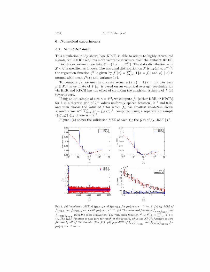
Figure 1(a) shows the validation-MSE of each fλ; the plot of ρX -MSE ‖f† −

Fig 1. (a) Validation-MSE of fKRR,λ and fKPCR,λ for ρX (x) ∝ x−1/2 vs. λ. (b) ρX -MSE of

fKRR,λ and fKPCR,λ vs. λ with ρX (x) ∝ x−1/2. (c) The estimated functions fKRR,λKRRand

fKPCR,λKPCRfrom the same simulation. The regression function f† is f†(x) =

∑5j=1 1{x =

j}. The KRR function is non-zero for much of the domain, while the KPCR function is zero

for nearly all of the domain (like f†). (d) ρX -MSE of fKRR,λKRRand fKPCR,λKPCR

for

ρX (x) ∝ x−α vs. α.


fλ‖2L2(ρX ) in Figure 1(b) has roughly the same shape, just shifted down by σ2 =

1/4. The selected λ is λKRR = 0.001534 for KRR, and λKPCR = 0.001573 for

KPCR. These choices of λ yield the final estimators, fKRR,λKRRand fKPCR,λKPCR

;

the ρX -MSE is 0.0034 for KRR, and 0.0003 for KPCR. In Figure 1(c), we plot

the functions fKRR,λKRRand fKPCR,λKPCR

to show the effect of regularization.The KRR function is non-zero for much of the domain, while the KPCR functionis zero for nearly all of the domain (like f†).

We repeat the above simulation for different marginal distributions ρX (x) ∝x−α, for 1/2 ≤ α ≤ 2, which imply different eigenvalue sequences {t2j}. Themean and standard deviation of the ρX -MSE’s over 10 repetitions are shown inFigure 1(d). This confirms KPCR’s to adapt to the regularity of f†, regardlessof the ambient RKHS; KRR requires more structure to achieve similar results.

6.2. Real data

We also compared KRR and KPCR using three “weighted degree” kernels de-signed for recognizing splice sites in genetic sequences (Sonnenburg, 2008).3 The3300 samples are divided into a training set (1000), validation set (1100), and

testing set (1200). For each kernel, we use the training data to compute fλ for λin a discrete grid of 210 equally-spaced values between 10−5 and 0.4, and selectthe value of λ on which the MSE of fλ on the validation set is smallest. TheMSE on the testing set and the intrinsic dimension dλ for the selected λ (on thetraining data) are as follows:

Kernel 1 Kernel 2 Kernel 3

MSE of fKRR,λKRR0.181452 0.172223 0.167745

MSE of fKPCR,λKPCR0.187059 0.168067 0.164159

dλKRR175.6879 373.0029 738.0712

dλKPCR170.9016 275.3560 581.1381

KRR outperforms KPCR with Kernel 1, where the intrinsic dimension of thekernel is low, while the reverse happens with Kernels 2 and 3, where the intrinsicdimensions are high. This resonates with our theoretical results, which suggestthat KRR requires low intrinsic dimension to perform most effectively.

7. Discussion

Our unified analysis for a general class of regularization families in nonparamet-ric regression highlights two important statistical properties. First, the resultsshow minimax optimality for this general class in several commonly studied set-tings, which was only previously established for specific regularization methods.Second, the results demonstrate the adaptivity of certain regularization families

3We use the first three kernels for the data obtained from http://mldata.org/repository/

data/viewslug/mkl-splice/.

http://mldata.org/repository/data/viewslug/mkl-splice/

http://mldata.org/repository/data/viewslug/mkl-splice/


to subspaces of the RKHS, showing that these techniques may take advantage ofadditional smoothness properties that the signal may possess. It is notable thatthe most well-studied family, KRR/Tikhonov regularization, does not possessthis adaptability property.

Appendix A: Proof of Theorem 1

To provide some intuition behind fλ and our proof strategy, consider the oper-ator T defined in (4), as applied to an element f ∈ H,

Tf =

∫X〈f,Kx〉HKx dρX (x) .

Observe that T is a “population” version of the operator TX , defined in (8).Unlike TX , T often has infinite rank; however, we still might expect that T ≈ TX

for large n, where the approximation holds in some suitable sense.We also have a large-n approximation for S∗

Xy. For f ∈ H,

〈f, S∗Xy〉H =

1

n

n∑i=1

yi〈f,Kxi〉H ≈∫Y×X

yf(x)dρ(y,x)

=

∫Xf†(x)f(x) dρX (x) = 〈f, f†〉L2(ρX ) = 〈f, Tf†〉H ,

where we have used the identity φj = tjψj to obtain the last equality. It fol-lows that S∗

Xy ≈ Tf†. Hence, to recover f† from y, it would be natural toapply the inverse of T to S∗

Xy. However, T is not invertible whenever it hasinfinite rank, and regularization becomes necessary. We thus arrive at the chainof approximations which help motivate fλ:

fλ = gλ(TX)S∗Xy ≈ gλ(T )Tf

† ≈ f† ,

where gλ(T ) may be viewed as an approximate inverse for a suitably chosenregularization parameter λ.

A.1. Bias-variance decomposition

The proof of Theorem 1 is based on a simple bias-variance decomposition of therisk of fλ. Let ε = (y1 − f†(x1), . . . , yn − f†(xn))

� ∈ Rn.

Proposition 2. The risk Rρ(fλ) has the decomposition

Rρ(fλ) = Bρ(fλ) + Vρ(fλ) , (13)

where Bρ(fλ) and Vρ(fλ) are defined as

Bρ(fλ) = E

[∥∥∥T 1/2{I − gλ(TX)TX}f†∥∥∥2H

],

Vρ(fλ) = E

[∥∥∥T 1/2gλ(TX)S∗Xε

∥∥∥2H

].


Our proof separately bounds the bias Bρ(fλ) and variance Vρ(fλ) terms from

Proposition 2. Taken together, these bounds imply a bound on Rρ(fλ).

A.2. Translation to vector and matrix notation

We first note that the Hilbert space H is isometric to �2(N) via the isometricisomorphism ι : H → �2(N), given by

ι :∞∑j=1

αjφj �→ (α1, α2, . . . )� (14)

(we take all elements of �2(N) to be infinite-dimensional column vectors). Us-ing this equivalence, we can convert elements of H and linear operators on Happearing in Proposition 2 into (infinite-dimensional) vectors and matrices, re-spectively, which we find simpler to analyze in the sequel.

Define the (infinite-dimensional) diagonal matrix

T = diag(t21, t22, . . . ) ,

and the vectorβ = (β1, β2, . . . )

� ∈ �2(N) ,

where βi = 〈f†, φi〉H. Next, define the n×∞ (random) matrices

Ψ = (ψj(xi))1≤i≤n;1≤j<∞ ,

Φ = ΨT = (φj(xi))1≤i≤n;1≤j<∞ .

Observe that

SX = Φ ◦ ι ,

S∗X = ι−1 ◦

(1

nΦ�

),

T = ι−1 ◦T ◦ ι .

Also, for 1 ≤ i ≤ n, let φiφ�i be the ∞ × ∞ matrix whose (j, j′)-th entry is

φj(xi)φj′(xi), and define

Σ =1

n

n∑i=1

φiφ�i =

1

nΦ�Φ .

Finally, let I = diag(1, 1, . . . ), and let ‖ · ‖ = ‖ · ‖�2(N) denote the norm on�2(N). In these matrix and vector notations, the bias-variance decompositionfrom Proposition 2 translates to the following:

Bρ(fλ) = E

[∥∥∥T1/2{I− gλ(Σ)Σ}β∥∥∥2] ,


Vρ(fλ) =1

n2E

[∥∥∥T1/2gλ(Σ)Φ�ε∥∥∥2] .

The boundedness of the kernel implies

tr(T) ≤ κ2 ,

‖φiφ�i ‖ ≤ κ2 ,

‖Σ‖ ≤ κ2 ,

where the norms are the operator norms in �2(N).

A.3. Probabilistic bounds

For 0 < r < 1, define the event

Ar =

{∥∥∥(T+ λI)−1/2(Σ −T)(T+ λI)−1/2∥∥∥ ≥ r

}, (15)

and let Acr denote its complement. Our bounds on bias Bρ(fλ) and variance

Vρ(fλ) are based on analysis in the event Acr (for a constant r). Therefore, we

also need to show that Acr has large probability (equivalently, show that Ar has

small probability).

Lemma 1. Assume that

supx∈X

∞∑j=1

t2(1−δ)j ψj(x)

2 ≤ κ2δ < ∞ (16)

for some 0 ≤ δ < 1, κ2δ > 0. Further assume that λ1−δ ≤ κ2

δ. If r ≥√κ2δ/(λ

1−δn) + κ2δ/(3λ

1−δn), then

P (Ar) ≤ 4dλ exp

(− λ1−δnr2

2κ2δ(1 + r/3)

).

Proof. The proof is an application of Lemma 5. Define, for 1 ≤ i ≤ n,

Xi =1

n(T+ λI)−1/2{φiφ

�i −T}(T+ λI)−1/2 ,

as well as Y =∑n

i=1 Xi. We have

Y = (T+ λI)−1/2(Σ −T)(T+ λI)−1/2 .

It is clear that E[Xi] = 0. Observe that

∞∑j=1

t2jt2j + λ

ψj(xi)2 ≤ max

j≥1

t2δjt2j + λ

∞∑j=1

t2(1−δ)j ψj(xi)

2


≤ κ2δ max

j≥1

t2δjt2j + λ

≤ κ2δ

λ1−δ, (17)

where the last inequality uses the inequality of arithmetic and geometric means.Therefore, by the assumption λ1−δ ≤ κ2

δ ,

‖Xi‖ ≤ 1

nmax

{‖(T+ λI)−1/2φiφ

�i (T+ λI)−1/2‖ ,

‖(T+ λI)−1/2T(T+ λI)−1/2‖}

=1

nmax

⎧⎨⎩

∞∑j=1

t2jt2j + λ

ψj(xi)2 , max

j≥1

t2jt2j + λ

⎫⎬⎭ ≤ κ2

δ

λ1−δn.

Moreover,

E[X2i ]

=1

n2E

[(T+ λI)−1/2φiφ

�i (T+ λI)−1φiφ

�i (T+ λI)−1/2 − (T+ λI)−2T2

]

=1

n2E

⎡⎢⎣⎧⎨⎩

∞∑j=1

t2jψj(xi)2

t2j + λ

⎫⎬⎭(T+ λI)−1/2φiφ

�i (T+ λI)−1/2 − (T+ λI)−2T2

⎤⎥⎦ .

Combining this with (17) gives

‖E[Y2]‖ ≤ κ2δ

λ1−δn

∥∥∥∥E[(T+ λI)−1/2φ1φ�1 (T+ λI)−1/2

]∥∥∥∥=

κ2δ

λ1−δn‖(T+ λI)−1T‖ ≤ κ2

δ

λ1−δn

and

tr(E[Y2]

)≤ κ2

δ

λ1−δntr

(E

[(T+ λI)−1/2φ1φ

�1 (T+ λI)−1/2

])

=κ2δ

λ1−δntr((T+ λI)−1T

)=

dλκ2δ

λ1−δn.

Applying Lemma 5 with V = R = κ2δ/(λ

1−δn) and D = dλ, gives

P(‖Y‖ ≥ r

)≤ 4dλ exp

(− λ1−δnr2

2κ2δ(1 + r/3)

).

Lemma 2.

E

[‖Σ −T‖2

]≤ 34κ4

n+

15κ4

n2.

Proof. The proof is an application of Lemma 6. Define, for 1 ≤ i ≤ n, Xi =1n (φiφ

�i −T), and also define Y =

∑ni=1 Xi, so Y = Σ −T. Clearly E[Xi] = 0

and ‖Xi‖ ≤ κ2/n. Additionally, since E[Y2] = n−1E[‖φ1‖2φ1φ

�1 −T2], we have

‖E[Y2]‖ ≤ κ4/n and tr(E[Y2]) ≤ κ4/n. The claim thus follows by applyingLemma 6 with V = κ4/n, D = 1, and R = κ2/n.


A.4. Bias bound

Lemma 3. Assume that β = Tζ/2α for some ζ ≥ 0 and that gλ has qualificationat least max{(ζ + 1)/2, 1}. For any 0 < r ≤ 1/2,

Bρ(fλ) ≤ 2ζ+2

1− r‖α‖2λζ+1 + t21 · ‖β‖2 · P (Ar)

+ 1{ζ > 1} · 8ζ2(1 + r)ζ−1

1− r· ‖α‖2 · ‖T+ λI‖ζ−1 · E

[‖Σ −T‖2

].

Proof. Define hλ(Σ) = I−Σgλ(Σ). Since |1− sgλ(s)| ≤ 1 for 0 < s ≤ κ2 and‖Σ‖ ≤ κ2, we have

‖hλ(Σ)‖ ≤ 1 .

Moreover, using β = Tζ/2α,

Bρ(fλ) = E

[∥∥∥T1/2hλ(Σ)β∥∥∥2]

≤ E

[∥∥∥T1/2hλ(Σ)Tζ/2∥∥∥2 · 1{Ac

d}]· ‖α‖2

+ ‖T1/2‖2 · ‖hλ(Σ)‖2 · ‖β‖2 · P (Ad)

≤ E

[∥∥∥T1/2hλ(Σ)Tζ/2∥∥∥2 · 1{Ac

d}]· ‖α‖2 + t21 · ‖β‖2 · P (Ad) .

The rest of the proof involves bounding E[‖T1/2hλ(Σ)Tζ/2‖2 ·1{Acr}]. We sep-

arately consider two cases: (i) ζ ≤ 1, and (ii) ζ > 1.Case 1: ζ ≤ 1. Since gλ has qualification at least 1, it follows that |(s+λ)(1−

sgλ(s))| ≤ 2λ for 0 < s ≤ κ2. This implies∥∥∥T1/2hλ(Σ)Tζ/2∥∥∥2 ≤

∥∥∥T1/2(Σ + λI)−1/2∥∥∥2 · ∥∥(Σ + λI)hλ(Σ)

∥∥2·∥∥∥Tζ/2(Σ + λI)−1/2

∥∥∥2≤ 4λ2 ·

∥∥∥T1/2(Σ + λI)−1T1/2∥∥∥

·∥∥∥Tζ/2(Σ + λI)−1Tζ/2

∥∥∥ . (18)

For 0 ≤ z ≤ 1,∥∥∥Tz/2(Σ + λI)−1Tz/2∥∥∥

=∥∥∥Tz/2

{(Σ −T) + (T+ λI)

}−1Tz/2

∥∥∥≤

∥∥∥Tz/2(T+ λI)−1/2∥∥∥2 · ∥∥∥(T+ λI)1/2

{(Σ −T) + (T+ λI)

}−1(T+ λI)1/2

∥∥∥=

∥∥∥Tz(T+ λI)−1∥∥∥ ·

∥∥∥∥(I− (T+ λI)−1/2(T−Σ)(T+ λI)−1/2)−1

∥∥∥∥


≤ λz−1 ·∥∥∥∥(I− (T+ λI)−1/2(T−Σ)(T+ λI)−1/2

)−1∥∥∥∥ , (19)

where the final inequality uses the fact sz/(s + λ) ≤ λz−1 for 0 ≤ z ≤ 1 ands ≥ 0. The final quantity in (19) is bounded above by λz−1/(1− r) on the eventAc

r, so applying this inequality with z = 1 and z = ζ to (18) gives

∥∥∥T1/2hλ(Σ)Tζ/2∥∥∥2 · 1{Ac

r} ≤ 4λ2 · 1

1− r· λ

ζ−1

1− r=

4λζ+1

(1− r)2.

So the bias in this case is bounded as

Bρ(fλ) ≤(

2

1− r

)2

· ‖α‖2 · λζ+1 + t21 · ‖β‖2 · P (Ar) .

Case 2: ζ > 1. We have∥∥∥T1/2hλ(Σ)Tζ/2∥∥∥2 ≤

∥∥∥T1/2(Σ + λI)−1/2∥∥∥2 · ∥∥∥(Σ + λI)1/2hλ(Σ)Tζ/2

∥∥∥2=

∥∥∥T1/2(Σ + λI)−1T1/2∥∥∥ ·

∥∥∥(Σ + λI)1/2hλ(Σ)Tζ/2∥∥∥2

≤∥∥∥T1/2(Σ + λI)−1T1/2

∥∥∥·∥∥∥(Σ + λI)1/2hλ(Σ)(T+ λI)ζ/2

∥∥∥2 . (20)

The first factor on the right-hand side of (20) can be bounded using (19) on theevent Ac

r. For the second factor, we have∥∥∥(Σ + λI)1/2hλ(Σ)(T+ λI)ζ/2∥∥∥

≤∥∥∥(Σ + λI)(ζ+1)/2hλ(Σ)

∥∥∥+

∥∥∥∥(Σ + λI)1/2hλ(Σ){(T+ λI)ζ/2 − (Σ + λI)ζ/2

}∥∥∥∥≤ (2λ)(ζ+1)/2 + 2λ1/2 ·

∥∥∥(T+ λI)ζ/2 − (Σ + λI)ζ/2∥∥∥ . (21)

Above, the first inequality is due to the triangle inequality, and the secondinequality uses the facts that gλ has qualification at least (ζ + 1)/2, and that(s+ λ)(z+1)/2 ≤ 2−1+(z+1)/2(s(z+1)/2 + λ(z+1)/2) for s ≥ 0 and z ≥ 1.

We now bound ‖(T + λI)ζ/2 − (Σ + λI)ζ/2‖ in terms of ‖T − Σ‖. First,observe that on the event Ac

r,

‖T−Σ‖ ≤ ‖T+ λI‖ · ‖(T+ λI)−1/2(T−Σ)(T+ λI)−1/2‖ < r · ‖T+ λI‖ ,

and, consequently,

‖Σ + λI‖ ≤ (1 + r) · ‖T+ λI‖ .

For any constant s > 0, define


As =1

(1 + r + s)‖T+ λI‖ · (T+ λI) ,

Bs =1

(1 + r + s)‖T+ λI‖ · (Σ + λI) .

Then, on the event Acr, applying Lemma 7 and Lemma 8 gives∥∥∥Aζ/2

s −Bζ/2s

∥∥∥ ≤ 2ζ ·∥∥∥A1/2

s −B1/2s

∥∥∥≤ ζ ·

{λ

(1 + r + s)‖T+ λI‖

}−1/2

· ‖As −Bs‖

= ζ ·{λ · (1 + r + s)‖T+ λI‖

}−1/2 · ‖T−Σ‖ .

Taking s → 0, it follows that on Acr,∥∥∥(T+ λI)ζ/2 − (Σ + λI)ζ/2

∥∥∥ ≤ ζ · λ−1/2 ·{(1 + r)‖T+ λI‖

}(ζ−1)/2

· ‖T−Σ‖ . (22)

Combining (21) and (22) gives∥∥(Σ + λI)1/2hλ(Σ)(T+ λI)ζ/2∥∥

≤ (2λ)(ζ+1)/2 + 2ζ ·{(1 + r)‖T+ λI‖

}(ζ−1)/2 · ‖T−Σ‖ .

Using this together with (19) in (20) and∥∥∥T1/2hλ(Σ)Tζ/2∥∥∥2 · 1{Ac

r}

≤ 1

1− r·((2λ)(ζ+1)/2 + 2ζ ·

{(1 + r)‖T+ λI‖

}(ζ−1)/2 · ‖T−Σ‖)2

.

Therefore

Bρ(fλ) ≤‖α‖21− r

·(2 · (2λ)ζ+1 + 8ζ2 ·

{(1 + r)‖T+ λI‖

}ζ−1 · E[‖T−Σ‖2

])+ t21 · ‖β‖2 · P (Ar).

A.5. Variance bound

Lemma 4. For any 0 < r < 1,

Vρ(fλ) ≤ 2

1− r· dλσ

2

n+

κ2σ2

λn· P (Ar) .

Proof. The assumption on ε = (ε1, . . . , εn)� implies E[εi] = 0, E[εiεj ] = 0 for

i �= j, and E[ε2i ] ≤ σ2. So, by Von Neumann’s inequality,

Vρ(fλ) =1

n2E

[∥∥∥T1/2gλ(Σ)Φ�ε∥∥∥2] ≤ σ2

nE

[tr(Tgλ(Σ)2Σ

)].


Using Von Neumann’s inequality together with tr(T) ≤ κ2 and gλ(s)2s ≤ 1/λ

for 0 < s ≤ κ2,

tr(Tgλ(Σ)2Σ

)≤ tr(T)

∥∥∥gλ(Σ)2Σ∥∥∥ ≤ κ2

λ.

Therefore

Vρ(fλ) ≤ σ2

nE

[tr(Tgλ(Σ)2Σ

)· 1{Ac

r}]+

κ2σ2

λn· P (Ar) .

Using Von Neumann’s inequality twice more, and (s + λ)gλ(s)2s ≤ 2 for 0 <

s ≤ κ2, we have

tr(Tgλ(Σ)2Σ

)= tr

(T(Σ + λI)−1(Σ + λI)gλ(Σ)2Σ

)≤ tr

(T(Σ + λI)−1

)∥∥∥(Σ + λI)gλ(Σ)2Σ∥∥∥

≤ 2tr(T(Σ + λI)−1

)= 2tr

(T(T+ λI)−1(T+ λI)1/2(Σ + λI)−1(T+ λI)1/2

)≤ 2tr

(T(T+ λI)−1

)∥∥∥(T+ λI)1/2(Σ + λI)−1(T+ λI)1/2∥∥∥

= 2dλ

∥∥∥∥(I− (T+ λI)1/2(T−Σ)−1(T+ λI)1/2)−1

∥∥∥∥ .This final quantity is bounded above by 2dλ/(1− r) on the event Ac

d.

A.6. Finishing the proof of Theorem 1

Using the bias-variance decomposition from Proposition 2, we apply the biasbound (Lemma 3) and variance bound (Lemma 4) to obtain a bound on therisk:

Rρ(fλ) = Bρ(fλ) + Vρ(fλ)

≤ 2ζ+2

1− r‖α‖2λζ+1 + t21 · ‖β‖2 · P (Ar)

+ 1{ζ > 1} · 8ζ2(1 + r)ζ−1

1− r· ‖α‖2 · (t21 + λ)ζ−1 · E

[‖Σ −T‖2

]

+2

1− r· dλσ

2

n+

κ2σ2

λn· P (Ar) .

Now set r = 1/2, and apply Lemma 1 to bound P (Ar). Note that the assumption(8/3+2

√5/3)κ2

δ/n ≤ λ1−δ satisfies the conditions on r in Lemma 1 for r = 1/2.Finally, apply Lemma 2 to bound E[‖Σ −T‖2].

Appendix B: Proof of Proposition 1

Let t21 ≥ t22 ≥ · · · ≥ 0 denote the eigenvalues of Σ and define T = diag(t21, t22, ...).

Let U be an orthogonal transformation satisfying Σ = UTU�. Additionally, let


hλ(t) = I{t ≤ λ}, define J = Jλ = inf{j; t2j > λ}, and write U = (U− U+),

where U− is the ∞× J matrix comprised of the first J columns of U , and U+

consists of the remaining columns of U . Finally, define T− = diag(t21, . . . , t2J),

T+ = diag(t2J+1

, t2J+2

, ...), and define the ∞× J matrix U− = (IJ 0)�, where

IJ is the J × J identity matrix.

Now consider the bias term Bρ(fKPCR,λ) = E

[∥∥∥T1/2hλ(Σ)β∥∥∥2], and observe

that ∥∥∥T1/2hλ(Σ)β∥∥∥2 =

∥∥∥T1/2U+U�+U−U

�−β

∥∥∥2 ≤ κ2∥∥∥U�

+U−

∥∥∥2 ‖f†‖2H .

Thus,

Bρ(fKPCR,λ) ≤ κ2‖f†‖2HE

(∥∥∥U�+U−

∥∥∥2 · 1{J ≥ J})+ κ2‖f†‖2HP (J < J) . (23)

Now we bound ‖U�+U−‖ on the event {J ≥ J}. We derive this bound from basic

principles, but it is essentially the Davis-Kahan inequality (Davis and Kahan,1970). Let D = Σ −T. Then

DU− = ΣU− −TU− = ΣU− − U−T−

andU�−DU+ = U�

−ΣU+ −T−U�−U+ = U�

−U+T+ −T−U�−U+.

Next notice that

‖D‖ ≥ ‖U�−DU+‖ ≥ ‖T−U

�−U+‖ − ‖U�

−U+T+‖≥ t2J‖U�

−U+‖ − (1− r)t2J‖U�−U+‖ = rt2J‖U�

−U+‖ .

Thus,

‖U�−U+‖ ≤ 1

rt2J‖D‖ (24)

on the event {J > J}.Next we bound P (J < J) = P (t2J ≤ λ) = P{t2J ≤ (1 − r)t2J}. By Weyl’s

inequality,|t2J − t2J | ≤ ‖D‖ = ‖Σ −T‖

and, by Lemma 5,

P(‖Σ −T‖ ≥ rt2J

)≤ 4 exp

(− nr2t4J2κ4 + 2κ2rt2J/3

),

provided rt2J ≥ κ2/n1/2 + κ2/(3n). Thus,

P (J < J) = P{t2J ≤ (1− r)t2J

}


≤ P (‖D‖ ≥ rt2J) ≤ 4 exp

(− nr2t4J2κ4 + 2κ2rt2J/3

). (25)

Combining (23)–(25) and using Lemma 2 gives

Bρ(fKPCR,λ) ≤ κ2

r2t4J‖f†‖2HE

[‖Σ −T‖2

]

+ 4κ2‖f†‖2H exp

(− nr2t4J2κ4 + 2κ2rt2J/3

)

≤ κ2

r2t4J‖f†‖2H

(34κ4

n+

15κ4

n2

)


(− nr2t4J2κ4 + 2κ2rt2J/3

).

Next, we combine this bound on Bρ(fKPCR,λ) with the variance bound Lemma4 (taking r = 0 in the lemma) to obtain

Rρ(fKPCR,λ) = Bρ(fλ) + Vρ(fλ)

≤ κ2

r2t4J‖f†‖2H

(34κ4

n+

15κ4

n2

)


(− nr2t4J2κ4 + 2κ2rt2J/3

)+

2dλσ2

n+

κ2σ2

λn

≤ κ2

r2t4J‖f†‖2H

(34κ4

n+

15κ4

n2

)


(− nr2t4J2κ4 + 2κ2rt2J/3

)+

3κ2σ2

(1− r)t2Jn

=1

n

{34κ6

r2t4J‖f†‖2H +

3κ2

(1− r)t2Jσ2

}

+ κ2‖f†‖2H

⎧⎨⎩ 15κ4

n2r2t4J+ 4 exp

(− nr2t4J2κ4 + 2κ2rt2J/3

)⎫⎬⎭ .

This completes the proof of the proposition.

Appendix C: Additional proofs and tools

C.1. Sums of random operators

Lemma 5. Let R > 0 be a positive real constant and consider a finite se-quence of self-adjoint Hilbert-Schmidt operators {Xi}ni=1 satisfying E[Xi] = 0


and ‖Xi‖ ≤ R almost surely. Define Y =∑n

i=1 Xi and suppose there areconstants V,D > 0 satisfying ‖E[Y2]‖ ≤ V and tr(E[Y2]) ≤ V D. For allt ≥ V 1/2 +R/3,

P(‖Y‖ ≥ t

)≤ 4D exp

(− t2

2(V +Rt/3)

).

Proof. This is a straightforward generalization of Tropp (2015, Theorem 7.7.1),using the arguments from Minsker (2011, Section 4) to extend from self-adjointmatrices to self-adjoint Hilbert-Schmidt operators.

Lemma 6. In the same setting as Lemma 5,

E

[‖Y‖2

]≤ (2 + 32D)V +

(2 + 128D

9

)R2 .

Proof. The proof is based on integrating the tail bound from Lemma 5:

E

[‖Y‖2

]=

∫ ∞

0

P(‖Y‖ ≥ t1/2

)dt

≤(V 1/2 +

R

3

)2

+

∫ ∞

(V 1/2+R3 )

24D exp

(− t

2(V +Rt1/2/3)

)dt

≤(V 1/2 +

R

3

)2

+

∫ 9V 2/R2

0

4D exp

(− t

4V

)dt

+

∫ ∞

9V 2/R2

4D exp

(−3t1/2

4R

)dt

=

(V 1/2 +

R

3

)2

+ 16V D

{1− exp

(− 9V

4R2

)}

+128R2D

9

{9V

4R2+ 1

}exp

(− 9V

4R2

)

=

(V 1/2 +

R

3

)2

+ 16V D

{1 + exp

(− 9V

4R2

)}+

128R2D

9exp

(− 9V

4R2

)

≤ (2 + 32D)V +

(2 + 128D

9

)R2 .

C.2. Differences of powers of bounded operators

Lemma 7. Let A and B be non-negative self-adjoint operators with ‖A‖ < 1and ‖B‖ < 1. For any γ ≥ 1,

‖Aγ −Bγ‖ ≤ 2γ‖A−B‖ .


Proof. The proof considers three possible cases for the value of γ: (i) γ is aninteger, (ii) 1 < γ < 2, and (iii) γ is a non-integer larger than two.

Case 1: γ is an integer. In this case, we have the following identity:

Aγ −Bγ =

γ∑j=1

Aj−1(A−B)Bγ−j .

So, by the triangle inequality,

‖Aγ −Bγ‖ ≤ ‖A−B‖γ∑

j=1

‖Aj−1‖‖Bγ−j‖ ≤ γ‖A−B‖ .

Case 2: 1 < γ < 2. Pick 0 < r < 1 such that ‖A‖ < r and ‖B‖ < r, and fix0 < t < (1− r)/2. Define At = A+ tI and Bt = B+ tI, and(

γ

k

)=

γ(γ − 1) · · · (γ − k + 1)

k!, k = 1, 2, . . . .

Then, using the power series (1 + s)γ = 1 +∑∞

k=1

(γk

)sk for −1 < s < 1,

Aγt −Bγ

t =∞∑k=1

(γ

k

){(At−I)k−(Bt−I)k} =

∞∑k=1

(γ

k

) k∑j=1

Aj−1(A−B)Bk−j .

Convergence is assured because ‖At−I‖ ≤ 1−t and ‖Bt−I‖ ≤ 1−t. Moreover,

‖Aγt −Bγ

t ‖ ≤ ‖A−B‖∞∑k=1

∣∣∣∣∣(γ

k

)∣∣∣∣∣k∑

j=1

‖At − I‖j−1‖Bt − I‖k−j

≤ ‖A−B‖∞∑k=1

∣∣∣∣∣(γ

k

)∣∣∣∣∣k(1− t)k−1

= γ‖A−B‖

⎧⎨⎩1 +

∞∑k=1

∣∣∣∣∣(γ − 1

k

)∣∣∣∣∣(1− t)k

⎫⎬⎭

= γ‖A−B‖{2− (1− (1− t))γ−1

}≤ 2γ‖A−B‖ .

Above, we have used the power series 1−(1−s)γ−1 =∑∞

k=1 |(γ−1k

)|sk at s = 1−t.

Taking t → 0 yields‖Aγ −Bγ‖ ≤ 2γ‖A−B‖ .

Case 3: γ is a non-integer larger larger than two. We can write γ = k + qfor an integer k ≥ 2 and real number 0 < q < 1. Applying the results from theprevious two cases gives

‖Aγ −Bγ‖ = ‖(Ak)γ/k − (Bk)γ/k‖ ≤ 2γ

k‖Ak −Bk‖ ≤ 2γ‖A−B‖ .


Lemma 8. Pick any real numbers r, γ ∈ (0, 1). Let A and B be non-negativeself-adjoint operators, each with spectrum contained in [r, 1). Then

‖Aγ −Bγ‖ ≤ γrγ−1‖A−B‖ .

Proof. Since ‖A− I‖ ≤ 1− r and ‖B− I‖ ≤ 1− r, the proof is similar to thatof Lemma 7:

‖Aγ −Bγ‖ ≤ γ‖A−B‖

⎧⎨⎩1 +

∞∑k=1

∣∣∣∣∣(γ − 1

k

)∣∣∣∣∣(1− r)k

⎫⎬⎭ = γrγ−1‖A−B‖ .

Above, we have used the power series (1−s)γ−1 = 1+∑∞

k=1 |(γ−1k

)|sk at s = 1−r

(which differs from the case in Lemma 7 because 0 < γ < 1).

References

Aronszajn, N. (1950). Theory of reproducing kernels. T. A. Math. Soc. 68337–404.

Bauer, F., Pereverzev, S. and Rosasco, L. (2007). On regularization al-gorithms in learning theory. J. Complexity 23 52–72.

Blanchard, G. and Mucke, N. (2016). Optimal rates for regularization ofstatistical inverse learning problems. arXiv preprint arXiv:1604.04054.

Caponnetto, A. and De Vito, E. (2007). Optimal rates for the regularizedleast-squares algorithm. Found. Comput. Math. 7 331–368. MR2335249

Caponnetto, A. and Yao, Y. (2010). Cross-validation based adaptationfor regularization operators in learning theory. Anal. Appl. 8 161–183.MR2646909

Carmeli, C., De Vito, E. and Toigo, A. (2006). Vector valued reproducingkernel Hilbert spaces of integrable functions and Mercer theorem. Anal. Appl.4 377–408.

Davis, C. and Kahan, W. M. (1970). The rotation of eigenvectors by a per-turbation. III. SIAM J. Numer. Anal. 7 1–46. MR0264450

Dhillon, P. S., Foster, D. P., Kakade, S. M. and Ungar, L. H. (2013). Arisk comparison of ordinary least squares vs ridge regression. J. Mach. Learn.Res. 14 1505–1511.

Dicker, L. H. (2016). Ridge regression and asymptotic minimax estimationover spheres of growing dimension. Bernoulli 22 1–37.

Engl, H. W.,Hanke, M. andNeubauer, A. (1996). Regularization of InverseProblems. Mathematics and Its Applications, Vol. 375, Springer.

Guo, Z. C., Lin, S. B. and Zhou, D. X. (2016). Learning theory of distributedspectral algorithms. Preprint.

Gyorfi, L., Kohler, M., Krzyzak, A. and Walk, H. (2002). A DistributionFree Theory of Nonparametric Regression. Springer.

Hsu, D., Kakade, S. M. and Zhang, T. (2014). Random design analysis ofridge regression. Found. Comput. Math. 14 569–600. MR3201956

http://www.ams.org/mathscinet-getitem?mr=2335249





Koltchinskii, V. (2006). Local Rademacher complexities and oracle inequali-ties in risk minimization. Ann. Stat. 34 2593–2656. MR2329442

Lin, S. B., Guo, X. and Zhou, D. X. (2016). Distributed learning with reg-ularized least squares. arXiv preprint arXiv:1608.03339.

Lo Gerfo, L., Rosasco, L., Odone, F., De Vito, E. and Verri, A. (2008).Spectral algorithms for supervised learning. Neural Comput. 7 1873–1897.

Mathe, P. (2005). Saturation of regularization methods for linear ill-posedproblems in Hilbert spaces. SIAM J. Numer. Anal. 42 968–973.

Minsker, S. (2011). On some extensions of Bernstein’s inequality for self-adjoint operators. arXiv preprint arXiv:1112.5448.

Neubauer, A. (1997). On converse and saturation results for Tikhonov regu-larization of linear ill-posed problems. SIAM J. Numer. Anal. 34 517–527.

Pinsker, M. S. (1980). Optimal filtration of square-integrable signals in Gaus-sian noise. Probl. Inf. Transm. 16 52–68.

Reed, M. and Simon, B. (1980). Methods of Modern Mathematical Physics;Volume 1, Functional Analysis. Academic Press.

Rosasco, L., De Vito, E. and Verri, A. (2005). Spectral methods for reg-ularization in learning theory. Tech. Rep. DISI-TR-05-18, Universita degliStudi di Genova, Italy.

Sonnenburg, S. (2008). Machine Learning for Genomic Sequence Analysis.Ph.D. thesis, Fraunhofer Institute FIRST. Supervised by K.-R. Muller andG. Ratsch.

Steinwart, I.,Hush, D. and Scovel, C. (2009). Optimal rates for regularizedleast squares regression. In Conference on Learning Theory.

Tropp, J. A. (2015). An introduction to matrix concentration inequalities.arXiv preprint arXiv:1501.01571.

Wasserman, L. (2006). All of Nonparametric Statistics. Springer.Zhang, T. (2005). Learning bounds for kernel regression using effective data

dimensionality. Neural Comput. 17 2077–2098.Zhang, Y., Duchi, J. C. and Wainwright, M. J. (2013). Divide and conquer

kernel ridge regression. In Conference on Learning Theory.


kernel ridge vs. principal component regression: minimax ...djhsu/papers/kernel-reg-ejs.pdfkernel...

Documents