journal of nepal mathematical society (jnms), vol. 2 ... · journal of nepal mathematical society...
TRANSCRIPT

Journal of Nepal Mathematical Society (JNMS), Vol. 2, Issue 1 (2019); A. A. Ansari, P. Kumar, M. Alam
Heterogeneous Oblate Primaries inPhoto-gravitational CR5BP with Kite Configuration
Abdullah A. Ansari1,3, Prashant Kumar2,3, Mehtab Alam3
1 Department of Mathematics, College of Science Al-Zulfi, Majmaah University, KSA2 Division of Mathematics, School of Basic and Applied Sciences,
Galgotias University, Greater Noida, U. P., India.3 International Center for Advanced Interdisciplinary Research (ICAIR)
Ratiya Marg, Sangam Vihar, New Delhi, India 110062
Correspondence to: Abdullah A. Ansari, Email: [email protected]
Abstract: This paper presents the investigation of the motion of infinitesimal body in the circular restrictedfive-body problem in which four bodies are taken as heterogeneous oblate spheroid with different densities inthree layers and sources of radiation pressure. These four primaries are moving on the circumference of acircle and form a kite configuration. After evaluating the equations of motion and Jacobi-integral, we studythe numerical part of the paper such as equilibria, zero-velocity curves and regions of motion. Finally, weexamine the stability of the equilibria and observed that all the equilibria are unstable.
Keywords: Heterogeneous oblate spheroid, CR5BP, Kite configuration, Equilibria, Zero-velocity curves,Stability
1 Introduction
The restricted problem is one of the attracting and interesting problem in the field of mechanics andastronomy due to its applications. The history of restricted problem starts before four centuries with Eulerand Lagranges in 1772. The restricted problem studied in three-body, four-body and five-body by manyresearchers with many perturbations as the different shapes of the primaries (oblate, triaxial, heterogeneous,finite straight segments etc.), solar radiation pressure, albedo effect, yarkovsky effects, drags, resonances,Coriolis and centrifugal forces, variable mass, etc. In the restricted three-body problem (R3BP), thetwo bodies, known as primaries, are moving in circular orbits around their common center of mass andthird body, known as infinitesimal body, are moving in space under the influence of these primaries but notinfluencing them. Many mathematicians have studied this problem with many perturbations as: Radzievskii[15, 16], Chernikov [9], Bhatnagar and Hallan [8], Singh and Lake [21], Suraj et al. [22, 23], Abouelmagdand Mostafa [2], Shalini et al. [19, 20], Ansari et al. [5], etc.
In the restricted four-body problem (R4BP), three-bodies are forming either Eulerian configuration orLagrangian configuration. And the fourth body is moving under the influence of these four primaries butnot affecting them. Many researchers have investigated this problem as: Kalvouridis et al. [10], Papadakis[14], Abdullah et al. [1], Baltagianis [7], Kumari and Kushvah [11], Ansari et al.[3, 4], etc.On the other hand, in the restricted five-body problem (R5BP), four primaries are moving in their mutualgravitational forces and the fifth body is moving under the influence of them but not influencing them.Many scientists have illustrated this problem as: Ollongren [13], Marchesin et al. [12], Shahbaz et al. [18],Shoaib et al. [17], Zotos et al. [24], Ansari et al. [6].
This paper is organized as follows: In the second section, we have determined the equations of motion andJacobian integral. In the third section, we have done the numerical works. In the fourth section, we haveexamined the stability of the equilibria. And finally, we have concluded the problem.
2 Description of the Problem and Equations of Motion
Here, we have considered the restricted five-body problem with circular kite configuration. In which fourbodies, taken as heterogeneous oblate spheroid with separate densities of three layers and also sources ofradiation, are placed at the circumference of the circle with radius R and also these four primaries areforming circular kite (P1P2P3P4) which has two triangles. P1P2P3 is an equilateral triangle with side `,
1
Heterogeneous Oblate Primaries in Photo-gravitational CR5BP with Kite Configuration
x
y
z
m (x, y, z)
O
m\2 (x
2 ,y2 ,0)
m3 (x3,y3,0)m\4 (x
4 ,y4 ,0)
m1 (x1,0,0)P1
P2
P3
P4
F1 r1F2r2
P
F3 r3
F4 r4
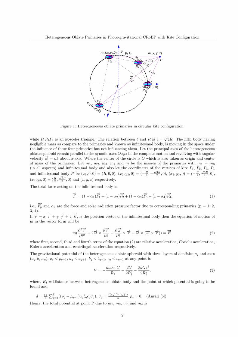
Figure 1: Heterogeneous oblate primaries in circular kite configuration.
while P1P3P4 is an isosceles triangle. The relation between ` and R is ` =√
3R. The fifth body havingnegligible mass as compare to the primaries and known as infinitesimal body, is moving in the space underthe influence of these four primaries but not influencing them. Let the principal axes of the heterogeneousoblate spheroid remain parallel to the synodic axes Oxyz in the complete motion and revolving with angularvelocity −→ω = nk about z-axis. Where the center of the circle is O which is also taken as origin and centerof mass of the primaries. Let m1, m2, m3, m4 and m be the masses of the primaries with m1 = m3
(in all aspects) and infinitesimal body and also let the coordinates of the vertices of kite P1, P2, P3, P4
and infinitesimal body P be (x1, 0, 0) = (R, 0, 0), (x2, y2, 0) = (−R2 ,−√
3R2 , 0), (x3, y3, 0) = (−R2 ,
√3R2 , 0),
(x4, y4, 0) = (R2 ,√
3R2 , 0) and (x, y, z) respectively.
The total force acting on the infinitesimal body is
−→F = (1− α1)
−→F1 + (1− α2)
−→F2 + (1− α3)
−→F3 + (1− α4)
−→F4, (1)
i.e.,−→Fp and αp are the force and solar radiation pressure factor due to corresponding primaries (p = 1, 2,
3, 4).
If −→r = x−→i + y
−→j + z
−→k , is the position vector of the infinitesimal body then the equation of motion of
m in the vector form will be
m(∂2−→r∂t2
+ 2−→ω × ∂−→r∂t
+∂−→ω∂t×−→r +−→ω × (−→ω ×−→r )) =
−→F . (2)
where first, second, third and fourth terms of the equation (2) are relative acceleration, Coriolis acceleration,Euler’s acceleration and centrifugal acceleration respectively.
The gravitational potential of the heterogeneous oblate spheroid with three layers of densities ρq and axes(aq, bq, cq), ρq < ρq+1, aq < aq+1, bq < bq+1, cq < cq+1 at any point is
V = −mass GR1
− dG
2R31
− 3dGz2
2R51
. (3)
where, R1 = Distance between heterogeneous oblate body and the point at which potential is going to befound and
d = 4π3
∑3q=1((ρq − ρq+1)aqbqcqσq), σq =
((aq)2−(cq)2)5 , ρ4 = 0. (Ansari [5])
Hence, the total potential at point P due to m1, m2, m3 and m4 is
2
Journal of Nepal Mathematical Society (JNMS), Vol. 2, Issue 1 (2019); A. A. Ansari, P. Kumar, M. Alam
V =
4∑p=1
(−mpG
rp− dpG
2r3p
− 3dpGz2
2r5p
), (4)
with,r2p = (x− xp)2 + (y − yp)2 + z2. (5)
To fix the units, the sum of the masses m1+ m2+ m3 + m4 = M = 1, the radius of the circle is consideredas unity i.e. R = 1, and unit of time is chosen in such a way that G = 1 and n = 1. Let µp =
mp
M , µ2 = µ
and µ4 = αµ, ⇒ µ1 = µ3 = 1−µ−αµ2 .
Hence from equation (2), the dimensionless equations of motion in the cartesian form will bex− 2y = ∂Ψ
∂x
y + 2x = ∂Ψ∂y
z = ∂Ψ∂z
(6)
where, ∂Ψ∂x ,
∂Ψ∂y and ∂Ψ
∂z are the partial derivatives of Ψ w.r.to x, y and z respectively, and
Ψ =1
2(x2 + y2) +
4∑p=1
βp(µprp
+dp2r3p
+3dpz
2
2r5p
),
βp = 1− αp, dp =4π
3
3∑q=1
((δpq − δpq+1)(Apq)
2Cpqσpq ),
Apq =apqR,Cpq =
cpqR, σpq =
((apq)2 − (cpq)
2)
5R2.(p = 1, 2, 3, 4)
After multiplying one by one in the system (6) with x, y, z respectively and adding, we get the Jacobi-Integral as
v2 = 2Ψ− C. (7)
where v2 = x2 + y2 + z2 is the velocity of the infinitesimal body and C is the Jacobi-Integral constant whichis conserved.
3 Analysis of the Problem
In this section, we have numerically investigated the equilibria, zero-velocity curves and regions of motion inthree planes (x-y, x-z and y-z planes) and shown the dynamical behaviour of the infinitesimal body. (In thecomplete investigation, we have taken: µ = 0.3, α = 0.01, d1 = d3 = 9.83933× 10⁻¹⁸, d2 = 1.58302× 10⁻⁷,d4 = 3.13153× 10⁻⁸, β1 = β2 = β3 = β4 = β.)(Ansari [5])
3.1 Evolution of equilibria
To evaluate the equilibrium points, we have to put right hand sides of system (6) equal to zero. i.e.,
∂Ψ
∂x= 0, (8)
∂Ψ
∂y= 0, (9)
∂Ψ
∂z= 0. (10)
After solving these equations by Mathematica software, we got figure 2, figure 3 and figure 4 in x-y, x-zand y-z plane respectively.
3
Heterogeneous Oblate Primaries in Photo-gravitational CR5BP with Kite Configuration
3.1.1 Equilibria in x-y plane
In this plane, we have plotted the equilibrium points at four different values of β (0.5, 0.8, 0.9, 1). Atβ = 0.5 and 0.8, we got four equilibrium points (L1, L2, L3, L4) in figures 2a and 2b respectively, whileβ = 0.9 and 1, we got one extra i.e. five equilibrium points (L1, L2, L3, L4, L5) in figures 2c and 2erespectively. Figures 2d and 2f are the zoomed figures of the figures 2c and 2e respectively. Red stars aredenoted as the locations of the photo-gravitational primaries (m1, m2, m3 and m4). From all the figures,we observed that equilibrium points are near the primaries except one. i.e., L1 is near m1, L3 is near m3,L4 is near m2, L5 is near m4 while L2 is near the origin. And also it is observed that as we increase thevalue of β these equilibrium points start moving away.
Therefore, we can say that these shapes of the primaries as heterogeneous and radiation factor have greatimpact as we know in the classical case of restricted three-body problem, researchers got five equilibriumpoints where three are collinear and two are non-collinear.
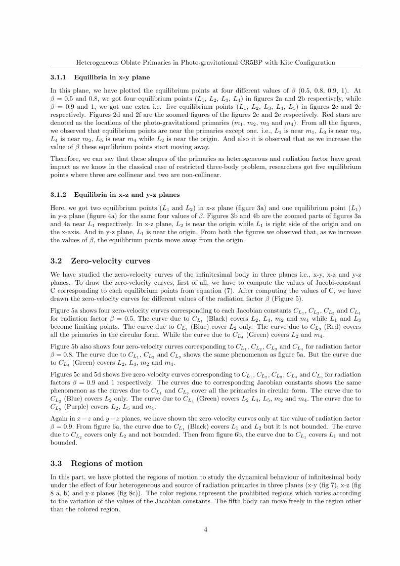
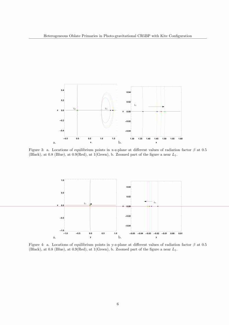
3.1.2 Equilibria in x-z and y-z planes
Here, we got two equilibrium points (L1 and L2) in x-z plane (figure 3a) and one equilibrium point (L1)in y-z plane (figure 4a) for the same four values of β. Figures 3b and 4b are the zoomed parts of figures 3aand 4a near L1 respectively. In x-z plane, L2 is near the origin while L1 is right side of the origin and onthe x-axis. And in y-z plane, L1 is near the origin. From both the figures we observed that, as we increasethe values of β, the equilibrium points move away from the origin.
3.2 Zero-velocity curves
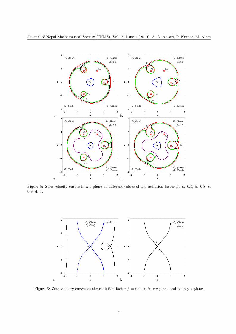
We have studied the zero-velocity curves of the infinitesimal body in three planes i.e., x-y, x-z and y-zplanes. To draw the zero-velocity curves, first of all, we have to compute the values of Jacobi-constantC corresponding to each equilibrium points from equation (7). After computing the values of C, we havedrawn the zero-velocity curves for different values of the radiation factor β (Figure 5).
Figure 5a shows four zero-velocity curves corresponding to each Jacobian constants CL1, CL2
, CL3and CL4
for radiation factor β = 0.5. The curve due to CL1(Black) covers L2, L4, m2 and m4 while L1 and L3
become limiting points. The curve due to CL2 (Blue) cover L2 only. The curve due to CL3 (Red) coversall the primaries in the circular form. While the curve due to CL4 (Green) covers L2 and m4.
Figure 5b also shows four zero-velocity curves corresponding to CL1, CL2
, CL3and CL4
for radiation factorβ = 0.8. The curve due to CL1
, CL2and CL3
shows the same phenomenon as figure 5a. But the curve dueto CL4 (Green) covers L2, L4, m2 and m4.
Figures 5c and 5d shows five zero-velocity curves corresponding to CL1, CL2
, CL3, CL4
and CL5for radiation
factors β = 0.9 and 1 respectively. The curves due to corresponding Jacobian constants shows the samephenomenon as the curves due to CL1
and CL3cover all the primaries in circular form. The curve due to
CL2 (Blue) covers L2 only. The curve due to CL4 (Green) covers L2 L4, L5, m2 and m4. The curve due toCL5 (Purple) covers L2, L5 and m4.
Again in x−z and y−z planes, we have shown the zero-velocity curves only at the value of radiation factorβ = 0.9. From figure 6a, the curve due to CL1
(Black) covers L1 and L2 but it is not bounded. The curvedue to CL2 covers only L2 and not bounded. Then from figure 6b, the curve due to CL1 covers L1 and notbounded.
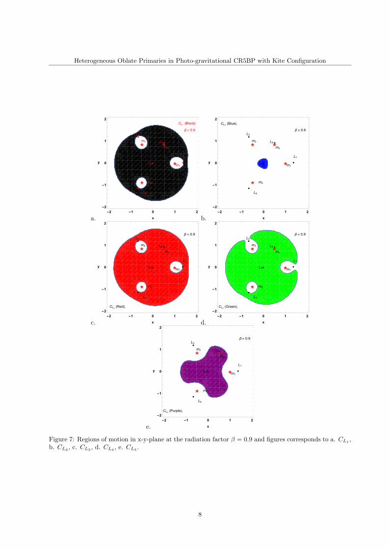
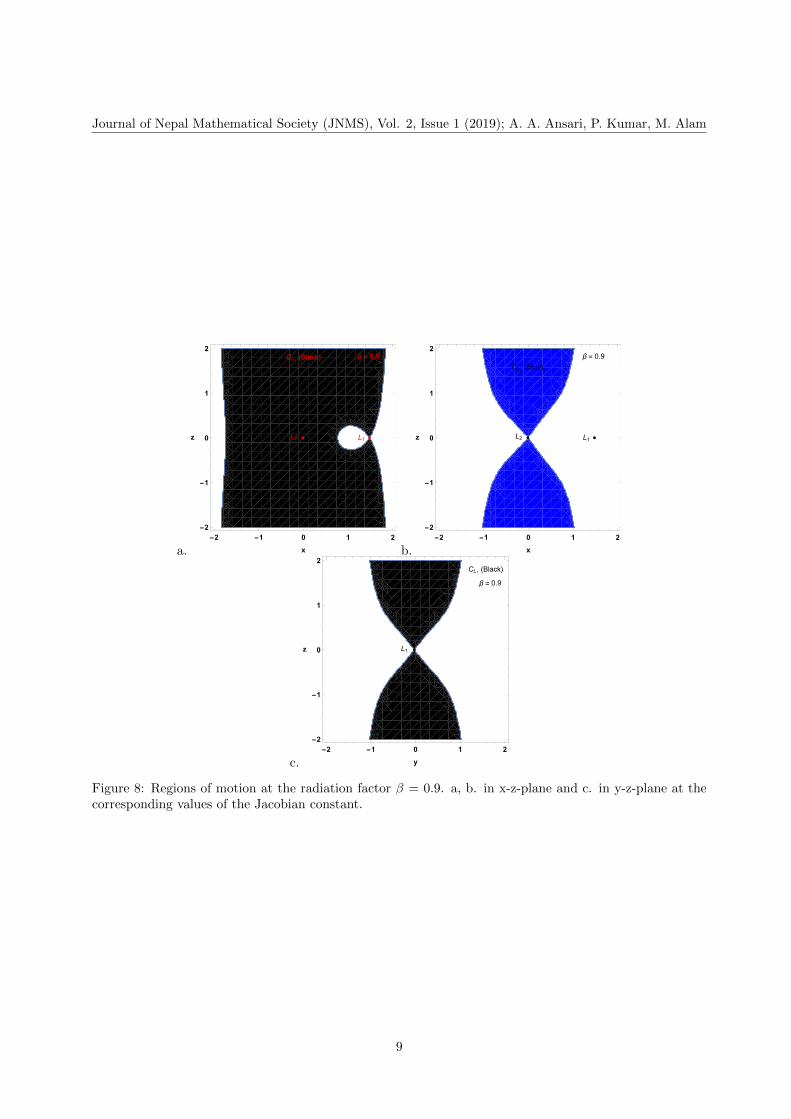
3.3 Regions of motion
In this part, we have plotted the regions of motion to study the dynamical behaviour of infinitesimal bodyunder the effect of four heterogeneous and source of radiation primaries in three planes (x-y (fig 7), x-z (fig8 a, b) and y-z planes (fig 8c)). The color regions represent the prohibited regions which varies accordingto the variation of the values of the Jacobian constants. The fifth body can move freely in the region otherthan the colored region.
4

Journal of Nepal Mathematical Society (JNMS), Vol. 2, Issue 1 (2019); A. A. Ansari, P. Kumar, M. Alam
a.
L1L2
L3
L4
β = 0.5
*m1
* m\2
*m3
*m\4
-2 -1 0 1 2-2
-1
0
1
2
x
y
b.
L1L2
L3
L4
β = 0.8
*m1
* m\2
*m3
*m\4
-2 -1 0 1 2-2
-1
0
1
2
x
y
c.
L1L2
L3
L4
L5
β = 0.9
*m1
* m\2
*m3
*m\4
-2 -1 0 1 2-2
-1
0
1
2
x
y
d.
L5
β = 0.9
*m\4
0.2 0.3 0.4 0.5 0.60.80
0.82
0.84
0.86
0.88
0.90
0.92
0.94
x
y
e.
L1L2
L3
L4
L5
β = 1
*m1
* m\2
*m3
*m\4
-2 -1 0 1 2-2
-1
0
1
2
x
y
f.
L5
β = 1
* m\4
0.2 0.3 0.4 0.5 0.60.80
0.82
0.84
0.86
0.88
0.90
0.92
0.94
x
y
Figure 2: Locations of equilibrium points in x-y-plane at different values of radiation factor β. a. at 0.5,b. at 0.8, c. at 0.9, d. zoomed part of figure c near L5, e. at 1 and f. zoomed part of figure e near L5.
5
Heterogeneous Oblate Primaries in Photo-gravitational CR5BP with Kite Configuration
a.
L1L2
-0.5 0.0 0.5 1.0 1.5
-0.4
-0.2
0.0
0.2
0.4
x
z
b.
L1
1.30 1.35 1.40 1.45 1.50 1.55 1.60
-0.04
-0.02
0.00
0.02
0.04
x
z
Figure 3: a. Locations of equilibrium points in x-z-plane at different values of radiation factor β at 0.5(Black), at 0.8 (Blue), at 0.9(Red), at 1(Green), b. Zoomed part of the figure a near L1.
a.
L1
-1.0 -0.5 0.0 0.5 1.0-1.0
-0.5
0.0
0.5
1.0
y
z
b.
L1
-0.05 -0.04 -0.03 -0.02 -0.01 0.00 0.01
-0.04
-0.02
0.00
0.02
0.04
y
z
Figure 4: a. Locations of equilibrium points in y-z-plane at different values of radiation factor β at 0.5(Black), at 0.8 (Blue), at 0.9(Red), at 1(Green), b. Zoomed part of the figure a near L1.
6
Journal of Nepal Mathematical Society (JNMS), Vol. 2, Issue 1 (2019); A. A. Ansari, P. Kumar, M. Alam
a.
L1L2
L3
L4
CL1 (Black)CL2 (Blue),
CL3 (Red), CL4 (Green)
β = 0.5
*m1
* m\2
*m3
*m\4
-2 -1 0 1 2-2
-1
0
1
2
x
y
b.
L1L2
L3
L4
CL1 (Black)CL2 (Blue),
CL3 (Red), CL4 (Green)
β = 0.8
*m1
* m\2
*m3
*m\4
-2 -1 0 1 2-2
-1
0
1
2
x
y
c.
L1
L2
L3
L4
L5
CL1 (Black)CL2 (Blue),
CL3 (Red),CL4 (Green)CL5 (Purple)
β = 0.9
*m1
* m\2
*m3
*m\4
-2 -1 0 1 2-2
-1
0
1
2
x
y
d.
L1L2
L3
L4
L5
CL1 (Black)CL2 (Blue),
CL3 (Red),CL4 (Green)CL5 (Purple)
β = 1.0
*m1
* m\2
*m3
*m\4
-2 -1 0 1 2-2
-1
0
1
2
x
y
Figure 5: Zero-velocity curves in x-y-plane at different values of the radiation factor β. a. 0.5, b. 0.8, c.0.9, d. 1.
a.
L1L2
β = 0.9CL1 (Black)CL2 (Blue),
-2 -1 0 1 2-2
-1
0
1
2
x
z
b.
L1
CL1 (Black)
β = 0.9
-2 -1 0 1 2-2
-1
0
1
2
y
z
Figure 6: Zero-velocity curves at the radiation factor β = 0.9. a. in x-z-plane and b. in y-z-plane.
7
Heterogeneous Oblate Primaries in Photo-gravitational CR5BP with Kite Configuration
a.
L1
L2
L3
L4
L5
CL1 (Black)
β = 0.9
*m1
* m\2
*m3
*m\4
-2 -1 0 1 2-2
-1
0
1
2
x
y
b.
L1
L2
L3
L4
L5
CL2 (Blue),
β = 0.9
*m1
* m2
*m3
*m4
-2 -1 0 1 2-2
-1
0
1
2
x
y
c.
L1
L2
L3
L4
L5
CL3 (Red),
β = 0.9
*m1
* m2
*m3
*m4
-2 -1 0 1 2-2
-1
0
1
2
x
y
d.
L1
L2
L3
L4
L5
CL4 (Green),
β = 0.9
*m1
* m2
*m3
*m4
-2 -1 0 1 2-2
-1
0
1
2
x
y
e.
L1
L2
L3
L4
L5
CL5 (Purple),
β = 0.9
*m1
* m2
*m3
*m4
-2 -1 0 1 2-2
-1
0
1
2
x
y
Figure 7: Regions of motion in x-y-plane at the radiation factor β = 0.9 and figures corresponds to a. CL1,
b. CL2, c. CL3
, d. CL4, e. CL5
.
8
Journal of Nepal Mathematical Society (JNMS), Vol. 2, Issue 1 (2019); A. A. Ansari, P. Kumar, M. Alam
a.
L1L2
β = 0.9CL1 (Black)
-2 -1 0 1 2-2
-1
0
1
2
x
z
b.
L1L2
β = 0.9
CL2 (Blue),
-2 -1 0 1 2-2
-1
0
1
2
x
z
c.
L1
CL1 (Black)
β = 0.9
-2 -1 0 1 2-2
-1
0
1
2
y
z
Figure 8: Regions of motion at the radiation factor β = 0.9. a, b. in x-z-plane and c. in y-z-plane at thecorresponding values of the Jacobian constant.
9
Heterogeneous Oblate Primaries in Photo-gravitational CR5BP with Kite Configuration
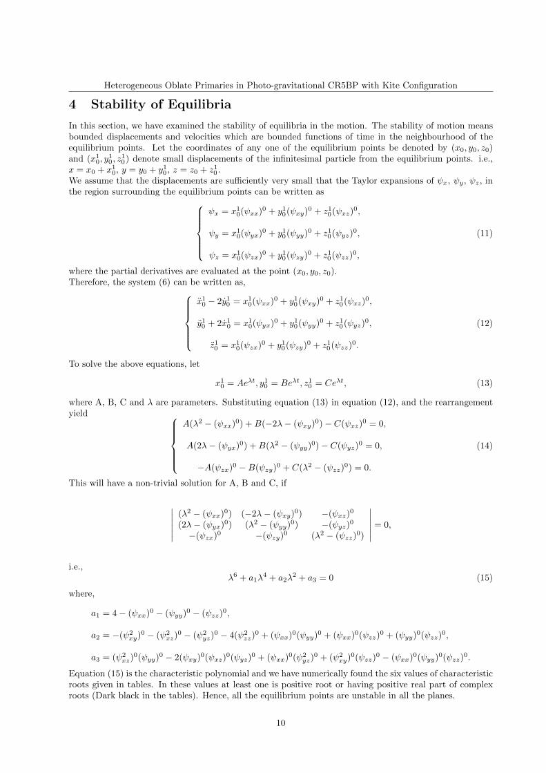
4 Stability of Equilibria
In this section, we have examined the stability of equilibria in the motion. The stability of motion meansbounded displacements and velocities which are bounded functions of time in the neighbourhood of theequilibrium points. Let the coordinates of any one of the equilibrium points be denoted by (x0, y0, z0)and (x1
0, y10 , z
10) denote small displacements of the infinitesimal particle from the equilibrium points. i.e.,
x = x0 + x10, y = y0 + y1
0 , z = z0 + z10 .
We assume that the displacements are sufficiently very small that the Taylor expansions of ψx, ψy, ψz, inthe region surrounding the equilibrium points can be written as
ψx = x10(ψxx)0 + y1
0(ψxy)0 + z10(ψxz)
0,
ψy = x10(ψyx)0 + y1
0(ψyy)0 + z10(ψyz)
0,
ψz = x10(ψzx)0 + y1
0(ψzy)0 + z10(ψzz)
0,
(11)
where the partial derivatives are evaluated at the point (x0, y0, z0).Therefore, the system (6) can be written as,
x10 − 2y1
0 = x10(ψxx)0 + y1
0(ψxy)0 + z10(ψxz)
0,
y10 + 2x1
0 = x10(ψyx)0 + y1
0(ψyy)0 + z10(ψyz)
0,
z10 = x1
0(ψzx)0 + y10(ψzy)0 + z1
0(ψzz)0.
(12)
To solve the above equations, let
x10 = Aeλt, y1
0 = Beλt, z10 = Ceλt, (13)
where A, B, C and λ are parameters. Substituting equation (13) in equation (12), and the rearrangementyield
A(λ2 − (ψxx)0) +B(−2λ− (ψxy)0)− C(ψxz)0 = 0,
A(2λ− (ψyx)0) +B(λ2 − (ψyy)0)− C(ψyz)0 = 0,
−A(ψzx)0 −B(ψzy)0 + C(λ2 − (ψzz)0) = 0.
(14)
This will have a non-trivial solution for A, B and C, if
∣∣∣∣∣∣(λ2 − (ψxx)0) (−2λ− (ψxy)0) −(ψxz)
0
(2λ− (ψyx)0) (λ2 − (ψyy)0) −(ψyz)0
−(ψzx)0 −(ψzy)0 (λ2 − (ψzz)0)
∣∣∣∣∣∣ = 0,
i.e.,λ6 + a1λ
4 + a2λ2 + a3 = 0 (15)
where,
a1 = 4− (ψxx)0 − (ψyy)0 − (ψzz)0,
a2 = −(ψ2xy)0 − (ψ2
xz)0 − (ψ2
yz)0 − 4(ψ2
zz)0 + (ψxx)0(ψyy)0 + (ψxx)0(ψzz)
0 + (ψyy)0(ψzz)0,
a3 = (ψ2xz)
0(ψyy)0 − 2(ψxy)0(ψxz)0(ψyz)
0 + (ψxx)0(ψ2yz)
0 + (ψ2xy)0(ψzz)
0 − (ψxx)0(ψyy)0(ψzz)0.
Equation (15) is the characteristic polynomial and we have numerically found the six values of characteristicroots given in tables. In these values at least one is positive root or having positive real part of complexroots (Dark black in the tables). Hence, all the equilibrium points are unstable in all the planes.
10

Journal of Nepal Mathematical Society (JNMS), Vol. 2, Issue 1 (2019); A. A. Ansari, P. Kumar, M. Alam
Radiation factor β Equilibria Corresponding Characteristic Roots0.5 1.364, 0.01 2.35721332, - 1.90974176 i, 1.90974176 i, - 2.35721332,
- 1.97720535 i, 1.97720535 i-0.0109, -0.0185 - 0.49941429 - 0.99999692 i, - 0.49941429 + 0.99999692 i,
0.49941429 + 0.99999692 i, 0.49941429 - 0.99999692 i,- 0.70628673 i, 0.70628673 i.
-0.67, 1.182 -2.42607259, - 1.95211201 i, 1.95211201 i, - 2.01868444 i,2.01868444 i, 2.42607259.
-0.67, -1.1582 -2.47287855, - 1.98117884 i, 1.98117884 i, - 2.04693700 i,2.04693700 i, 2.47287855.
0.8 1.454, 0.001 -2.07603417, - 1.74172796 i, 1.74172796 i, - 1.81005567 i,1.81005567 i, 2.07603417.
-0.0109, -0.0195 - 0.63168818 - 0.99998827 i, - 0.63168818 + 0.99998827 i,0.63168818 + 0.99998827 i, 0.63168818 - 0.99998827 i,
- 0.89336770 i, 0.89336770 i.-0.72, 1.267 - 2.04385981, - 1.72284988 i, 1.72284988 i, - 1.79141038 i,
1.79141038 i, 2.04385981.-0.72, -1.242 - 2.04040081, - 1.72107142 i, 1.72107142 i, - 1.78916186 i,
1.78916186 i, 2.04040081.0.9 1.454, 0.001 - 2.25221769, - 1.84738147 i, 1.84738147 i, - 1.91302538 i,
1.91302538 i, 2.25221769.-0.0109, -0.0195 - 0.67000480 - 0.99998566 i, - 0.67000480 + 0.99998566 i,
0.67000480 + 0.99998566 i, 0.67000480 - 0.99998566 i,- 0.94755953 i, 0.94755953 i.
-0.732, 1.28367 - 2.02696867, - 1.71332677 i, 1.71332677 i, - 1.78132347 i,1.78132347 i, 2.02696867.
-0.712, -1.2682 - 2.02753039, - 1.71398738 i, 1.71398738 i, - 1.78131488 i,1.78131488 i, 2.02753039.
0.51, 0.91 - 7.62240806, - 5.41881682 i, 5.41881682 i, - 5.46177308 i,5.46177308 i, 7.62240806.
1.0 1.514, 0.001 - 1.86697631, - 1.62146153 i, 1.62146153 i, - 1.69010738 i,1.69010738 i, 1.86697631.
-0.0109, -0.0195 - 0.70624540 - 0.99998289 i, - 0.70624540 + 0.99998289 i,0.70624540 - 0.99998289 i, 0.70624540 + 0.99998289 i,
- 0.99881545 i, 0.99881545 i.-0.732, 1.29367 - 2.10256574, - 1.75820925 i, 1.75820925 i, - 1.82468704 i,
1.82468704 i, 2.10256574.-0.732, -1.2682 - 2.09086345, - 1.75158070 i, 1.75158070 i, - 1.81758933 i,
1.81758933 i, 2.09086345.0.51, 0.91 - 7.62240806, - 5.41881682 i, 5.41881682 i, - 5.46177308 i,
5.46177308 i, 7.62240806.
Table 1: Corresponding characteristic roots of equilibria for the different values of radiation factor β inx-y-plane.
11
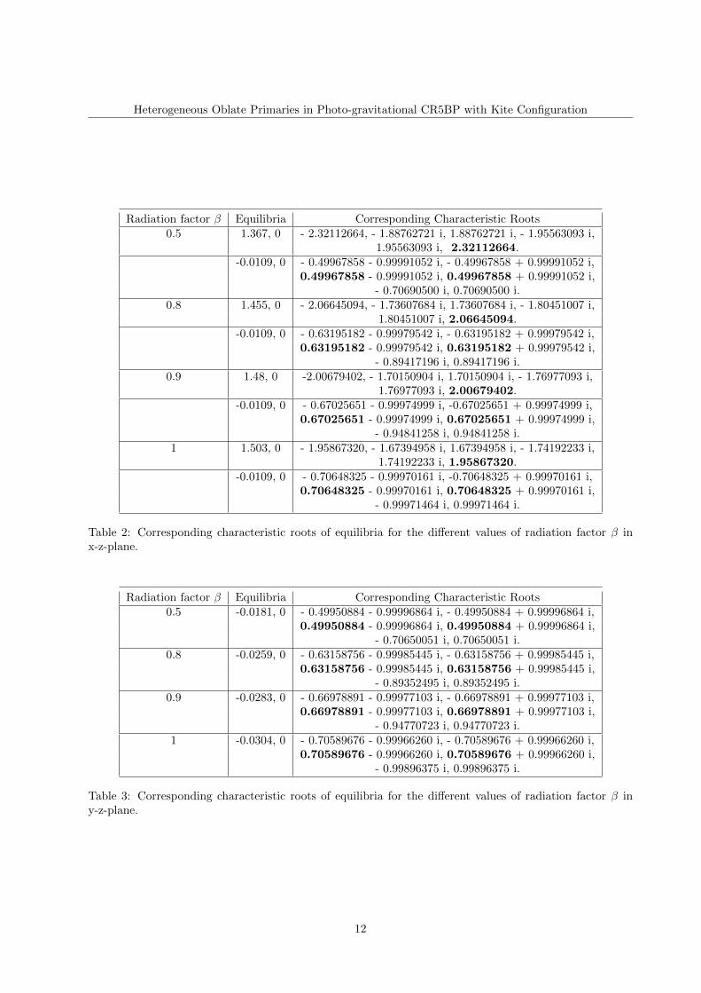
Heterogeneous Oblate Primaries in Photo-gravitational CR5BP with Kite Configuration
Radiation factor β Equilibria Corresponding Characteristic Roots0.5 1.367, 0 - 2.32112664, - 1.88762721 i, 1.88762721 i, - 1.95563093 i,
1.95563093 i, 2.32112664.-0.0109, 0 - 0.49967858 - 0.99991052 i, - 0.49967858 + 0.99991052 i,
0.49967858 - 0.99991052 i, 0.49967858 + 0.99991052 i,- 0.70690500 i, 0.70690500 i.
0.8 1.455, 0 - 2.06645094, - 1.73607684 i, 1.73607684 i, - 1.80451007 i,1.80451007 i, 2.06645094.
-0.0109, 0 - 0.63195182 - 0.99979542 i, - 0.63195182 + 0.99979542 i,0.63195182 - 0.99979542 i, 0.63195182 + 0.99979542 i,
- 0.89417196 i, 0.89417196 i.0.9 1.48, 0 -2.00679402, - 1.70150904 i, 1.70150904 i, - 1.76977093 i,
1.76977093 i, 2.00679402.-0.0109, 0 - 0.67025651 - 0.99974999 i, -0.67025651 + 0.99974999 i,
0.67025651 - 0.99974999 i, 0.67025651 + 0.99974999 i,- 0.94841258 i, 0.94841258 i.
1 1.503, 0 - 1.95867320, - 1.67394958 i, 1.67394958 i, - 1.74192233 i,1.74192233 i, 1.95867320.
-0.0109, 0 - 0.70648325 - 0.99970161 i, -0.70648325 + 0.99970161 i,0.70648325 - 0.99970161 i, 0.70648325 + 0.99970161 i,
- 0.99971464 i, 0.99971464 i.
Table 2: Corresponding characteristic roots of equilibria for the different values of radiation factor β inx-z-plane.
Radiation factor β Equilibria Corresponding Characteristic Roots0.5 -0.0181, 0 - 0.49950884 - 0.99996864 i, - 0.49950884 + 0.99996864 i,
0.49950884 - 0.99996864 i, 0.49950884 + 0.99996864 i,- 0.70650051 i, 0.70650051 i.
0.8 -0.0259, 0 - 0.63158756 - 0.99985445 i, - 0.63158756 + 0.99985445 i,0.63158756 - 0.99985445 i, 0.63158756 + 0.99985445 i,
- 0.89352495 i, 0.89352495 i.0.9 -0.0283, 0 - 0.66978891 - 0.99977103 i, - 0.66978891 + 0.99977103 i,
0.66978891 - 0.99977103 i, 0.66978891 + 0.99977103 i,- 0.94770723 i, 0.94770723 i.
1 -0.0304, 0 - 0.70589676 - 0.99966260 i, - 0.70589676 + 0.99966260 i,0.70589676 - 0.99966260 i, 0.70589676 + 0.99966260 i,
- 0.99896375 i, 0.99896375 i.
Table 3: Corresponding characteristic roots of equilibria for the different values of radiation factor β iny-z-plane.
12
Journal of Nepal Mathematical Society (JNMS), Vol. 2, Issue 1 (2019); A. A. Ansari, P. Kumar, M. Alam
5 Conclusion
In this study, we have performed the behavior of the motion of infinitesimal body in the restricted five-bodyproblem under the assumption that the four primaries are heterogeneous in shapes and sources of radiationpressure. After evaluating the equations of motion, we numerically execute the equilibria, zero-velocitycurves and regions of motion in three planes i.e. x-y, x-z and y-z planes, for different values of radiationfactor β. In the x-y plane, at β = 0.5 and 0.8, we got four equilibria but at 0.9 and 1, we got five equilibria.In the x-z plane, we got two equilibria at β = 0.9. And in the y-z plane, we got only one equilibrium point atβ = 0.9. As far as zero-velocity and regions of motion are concerned, we have plotted these in three planesand explained in detail in the concerning sections. On the other hand, for stability, we have examined itnumerically and found that all the equilibria are unstable.
References
[1] Abdullah, Ahmad, I. and Bhatnagar, K.B., 2009, Periodic orbits of collision in the plane circularproblem of four bodies with one of the primaries as an oblate body, Global Sci-Tech, Al-Falah’sJournal of Science and Technology, 1(1), Jan-March.
[2] Abouelmagd, E. I. and Mostafa, A., 2015, Out-of-plane equilibrium points locations and forbiddenmovement regions in the restricted three-body problem with variable mass, Astrophysics Space Sci.,357, 58, DOI 10.1007/s10509-015-2294-7.
[3] Ansari, A. A., 2016, The Photogravitational Circular Restricted Four-body Problem with VariableMasses, Journal of Engineering and Applied Sciences(Majmaah University), 3(2), November.
[4] Ansari, A. A., Kellil, R. and Alhussain, Z., 2017, The effect of perturbations on the circular restrictedfour-body problem with variable masses, Journal of Mathematics and Computer Science, 17(3), 365-377.
[5] Ansari, A. A., Alhussain, Z. and Prasad, S., 2018, The circular restricted three-body problem whenboth the primaries are heterogeneous spheroid of three layers and infinitesimal body varies it’s mass,Journal Of Astrophysics and Astronomy, 39, 57.
[6] Ansari, A. A. and Alhussain, Z., 2018, The restricted five-body problem with cyclic kite configuration,Accepted for publication in Journal of Dynamical Systems and Geometric Theories.
[7] Baltagiannis, A.N. and Papadakis, K.E., 2011, Equilibrium points and their stability in therestricted four-body problem, International Journal of Bifurcation and Chaos, 21, 2179, DOI10.1142/S0218127411029707.
[8] Bhatnagar, K. B. and Hallan, P. P., 1978, Effect of perturbations in coriolis and centrifugal forces onthe stability of equilibrium points in the restricted problem, Celest. Mech. Dyn. Astr., 18, 105–112.
[9] Chernikov, Yu. A., 1970, The photogravitational restricted three-body problem, Soviat Astron A. J.,14, 1.
[10] Kalvouridis, T.J., Arribas, M. and Elipe, A., 2007, Parametric evolution of periodic orbits inthe restricted four-body problem with radiation pressure, Planet. Space Sci., 55, 475-493, DOI10.1016/j.pss.2006.07.005.
[11] Kumari, R. and Kushvah, B. S., 2014, Stability regions of equilibrium points in the restricted four-bodyproblem with oblateness effects, Astrophysics and Space Sci., 349, 693-704.
[12] Marchesin, M. and Vidal, C., 2013, Special restricted rhomboidal five-body problem and horizontalstability of its periodic solutions, Celest. Mech. Dyn. Astro., 115, 261-279, DOI 10.1007/s10569-012-9462-7.
[13] Ollongren, A., 1988, On a particular restricted five-body problem: An analysis with computer algebra,J. Symbolic computation, 6, 117-126.
13
Heterogeneous Oblate Primaries in Photo-gravitational CR5BP with Kite Configuration
[14] Papadakis, K.E., 2007, Asymptotic orbits in the restricted four-body problem, Planet. Space Sci., 55,1368–1379, DOI 10.1016/j.pss.2007.02.005.
[15] Radzievskii, V. V., 1950, The restricted problem of three bodies taking account of light pressure, Akad.Nauk. USSR, Astron. J., 27, 250.
[16] Radzievskii, V. V., 1953, The photo-gravitational restricted three-body problem, Astron. Z., 30(3),265.
[17] Shoaib, M., Kashif, A.R. and Csillik, I.S., 2017, On the planar central configurations of rohomboidaland triangular four-and five-body problems, Astrophys Space Sci., 362, 182.
[18] Shahbaz, Ullah M., Bhatnagar, K.B. and Hassan, M.R., 2014, Sitnikov problem in the cyclic kiteconfiguration, Astrophys Space Sci., 354, 301-309.
[19] Shalini, K., Ansari, A. A., and Ahmad, F., 2016, Existence and Stability of L4 of the R3BP Whenthe Smaller Primary is a Heterogeneous Triaxial Rigid Body with N Layers, J. Appl. Environ. Biol.Sci., 6(1), 249-257.
[20] Shalini, K., Suraj, M. S. and Aggarwal, R., 2017, The Non-linear stability of L4 in the R3BP when thesmaller primary is a Heterogeneous Spheroid, J. of Astronaut Sci., 64(1), 18-49, DOI 10.1007/s40295-016-0093-1.
[21] Singh, J. and Leke, O., 2010, Stability of photogravitational restricted three body problem with variablemass, Astrophysics Space Sci., 326 (2), 305-314.
[22] Suraj, M. S., Hassan, M. R. and Asique, M. C., 2014, The Photo-Gravitational R3BP when thePrimaries are Heterogeneous Spheroid with Three Layers, J. of Astronaut Sci., 61, 133-155, DOI10.1007/s40295-014-0026-9.
[23] Suraj, M. S., Aggarwal, R., Shalini, K. and Asique, M. C., 2018, Out-of-Plane Equilibrium points andregions of motion in Photogravitational R3BP when the Primaries are Heterogeneous Spheroid withThree Layers, New Astronomy, 63(8), 15-26.
[24] Zotos, E.E. and Suraj, M.S., 2018, Basins of attraction of equilibrium points in the planar circularrestricted five-body problem, Astrophys Space Sci., 363, 20, http:doi.org/10.1007/s10509-017-3240-7.
14