journal of empirical finance the forward discount … · portfolio-balance models of risk premiums....

Journal of EMPIRICAL FINANCE

E L S E V I E R Journal of Empirical Finance 3 (1996) 123-192

The forward discount anomaly and the risk premium: A survey of recent evidence

Charles Engel Department (~f Economics. University of Washington. Seattle. WA 98195. USA

NBER, Cambridge MA, USA

Received 20 September 1995

Abstract

Forward exchange rate unbiasedness is rejected in tests from the current floating exchange rate era. This paper surveys advances in this area since the publication of Hodrick's (1987) survey. It documents that the change in the future exchange rate is generally negatively related to the forward discount. Properties of the expected forward forecast error are reviewed. Issues such as the relation of uncovered interest parity to real interest parity, and the implications of uncovered interest parity for cointegration of various quantities are discussed. The modeling and testing for risk premiums is surveyed. Included in this area are tests of the consumption CAPM, tests of the latent variable model, and portfolio-balance models of risk premiums. General equilibrium models of the risk premium are examined and their empirical implications explored. The survey does not cover the important areas of learning and peso problems, tests of rational expectations based on survey data, or the models of irrational expectations and speculative bubbles.

JEL classification: F30

Keywords: Forward discount anomaly; Risk premiums; Models of risk premiums; Testing efficiency of forward markets

I. I n t r o d u c t i o n

In 1987, Rober t Hodr ick surveyed the tests o f e f f ic iency of forward markets for foreign exchange . At that t ime, the most puzz l ing aspect o f forward market

behav ior was that there appeared to be a large condi t ional bias i f the forward rate

0927-5398/96/$15.00 © 1996 Elsevier Science B.V. All rights reserved SSDIO927-5398(95)OOOI6-X

124 c. Enge I / Jou rna I o! Empirical Finance 3 (1996) 123-192

were used to forecast the future spot exchange rate. Hodrick concluded, " W e do not yet have a model of expected returns that fits the da ta" (p. 157).

This paper is intended as a survey of the developments in the empirical literature on forward market efficiency since the publication of Hodr ick ' s book. Dozens of papers have been written which explore this issue. This paper is limited in scope. We will examine a few of the major findings, and provide a framework for judging the significance of recent research.

The conclusions of the survey can be summarized as: First, empirical tests routinely reject the null hypothesis that the forward rate is a condit ionally unbiased predictor of future spot rates. Second, models of the risk premium have been unsuccessful at explaining the magnitude of this failure of unbiasedness.

Some progress has been made toward understanding the empirical findings when one allows for peso problems, learning, and possibly a group of agents whose irrational expectations lead to speculative bubbles through a bandwagon effect. A likely outcome of future research is that risk premia, peso problems, learning, irrational speculative bubbles, as well as the effects of small transactions costs will be found to play a role in explaining forward rate bias. However, this survey is limited only to those studies which have assumed rational expectations and attempted to attribute the forward rate bias to a foreign exchange risk premium.

A useful starting point is to consider the regression of the change in the log of the spot exchange rate on the forward discount (expressed in log form):

s , + , - s, = ~, + 1 3 ( f , - s , ) + . , + , . ( 1 )

where s t is the log of the spot price of foreign currency at time t, f , is the log of the one-period forward exchange rate at time t, and IIt is the regression error. This regression appears frequently in the literature. Generally, the null hypothesis tested is that a = 0, 13 = 1 and u,+ 1 has a conditional mean of zero. Under that null hypothesis, the log of the forward rate provides an unbiased forecast of the log of

i the future spot exchange rate. Let ~ represent the estimate of 13. If the estimator is consistent, we have

Cov(g - s , , s , + , - s , )

p l i m ( ~ ) = 13 = V a r ( f , - so) '

where VarO refers to variance, and CovO is covariance. If expectations are rational, then

s,+ l - s, = E , ( s , + l ) - st + ~ , + ,

where E t represents the mathematical expectation conditional on information

i See Section 2.2 below, which relates the null hypothesis to risk-neutral behavior of investors.

C. Engel / Journal of Empirical Finance 3 (1996) 123-192 125

available to the market at time t, and with %+ t uncorrelated with time t variables. In that case,

C o v ( f r - s,, s¢+, - st) = C o v ( f t - s , , E , ( s , + , ) - st).

We shall define

rp re =- f ~ - E t ( s , + , ) . (2)

The term rpf e refers to the foreign exchange risk premium. The notion is that under risk neutrality, agents would drive f , into equality with E, (s ,+ 1), so that expected profits from forward market speculation would be zero. If f, > E,(st+ i), then the investor incurs a premium from buying the foreign currency forward at time t relative to its expected price on the spot market at time t + 1. Later we shall examine more closely the meaning of 'risk premium' in this context. The superscript ' re ' refers to the risk premium when expectations are rational.

Since, from Eq. (2) we have that

E,(s ,+ t) - s, = f , - s , - rpf ~,

we can write

C o v ( f , - s , , E , ( s , + , ) - - s t )

= Var( f , - s,) - C o v ( f , - s, , rp~, ~)

= Var( f , - s,) - Cov(E, ( s,+ l ) - s, , rpf ~) - Var(rprt~).

We have

pl im(~) = 1 - 13rp,

where

C o v ( E , ( s , + , ) - s , , rp, ~) + Var( rPt e)

13,,, = Var ( f , - s,)

This formulation is interesting because, in fact, when Eq. (1) is estimated, a consistent finding is that 13 < 1, which means 13rp > 0. Bilson (1981) and Fama (1984) document the finding that ~ < 1. Many recent studies have confirmed that finding, not just for dollar exchange rates, but for a large number of exchange rates and time periods (see, for example, Bekaert and Hodrick, 1993; Backus et al., 1993; Mark et al., 1993). Froot (1990) notes that the average value of ~ over 75 published estimates is - 0 . 8 8 . Only a few of the estimates are greater than zero, and none is greater than 1.

It appears from the definition of 13,e that low values of ~ can be explained under rational expectations if Var(rp r~) is large. But, as Fama (1984) notes, to explain a value of 13 < 0 , we need C o v ( E , ( s , + l ) - s , , r p ~ ) < O in models of rational expectations. Specifically, 13 < 0 implies

Var ( f , - s,) < Cov (E,( s, +t ) - st , rp~, ~) + Var( rpr, ~ ) .

126 C. Engel / Journal ~f Empirical Finance 3 (1996) 123-192

Since

Var(f , - s,) = Var( rpt ¢) + 2Cov(E,( st+ ' ) - s , , rp; ~ )

+ Var(Et(s ,+ 1) - s t ) ,

13 < 0 requires

C o v ( E t ( S , + l ) - s t , rprt e) + V a r ( E t ( s / + t ) - s t ) < O.

From this equation, 13 < 0 implies Cov(Et(s t+ 1) - strp re) < 0, and Var(rpt e) > Var(Et(s,+ l) - s t ) . As we shall discuss below, models of the foreign exchange risk premium should be consistent with these two inequalities.

Until now we have considered the estimate of 13 in large samples, where we have a consistent estimator. In finite samples we can write

= C o y ( f , - s , . s , . , - s , )

V a r ( f / - s,)

where the overbar refers to an estimate. Following the derivations above,

- ~ = 1 - - ~ r t - - ~ ......

where

~.,.,. = C ° v ( f t - s t ' E ' ( s t + ' ) - s t + , )

Var(f~ - s,)

~.,., represents the deviation of the estimate of 13 in a particular sample from its probability limit. ~ may not equal 13 because of small-samplebias, or because of sampling variation. When the estimator of 13 is consistent, 13.~s is zero in large samples (that is, pl im(~,,) = 0.)

The literature discusses two reasons why ~.~, might not be zero in a particular sample. Both situations arise when agents' information set differs from that of the econometrician. First, consider the case of a change in regime for the stochastic process driving s t . The agent may use information efficiently, but information about the new stochastic process for s t is revealed only gradually. Over a period of time there could be a positive covariance of ft - s, and E t ( s t + I ) - St+ l, and thus a positive value for 13.~..,.. The econometrician has more information than the agent did at the beginning of the sample, so the econometrician recognizes this positive covariation but the agent could not have foreseen it. This covariance goes to zero as agents learn more about the stochastic process for st. An alternative case is one in which agents have more information than the econometrician. Specifi- cally, agents may form their expectations using the correct distribution for exchange rates, but the ex post sample does not contain all of the events that agents think will occur with the correct frequency of occurrence. For example, suppose over some sub-period in our sample agents rationally expect a large increase in s, but that increase does not occur. Then, we would see high values of

C. Engel / Journal t~f Ernpirical Finance 3 (1996) 123-192 127

f t - st at the same time we seen high values of El(st+ l) - st+ i. Thus, we might find a positive value for ~.~.~. This is an example of the 'peso problem' . Again, in large samples this covariance goes to zero if agents' expectations are rational.

Now, suppose that the market ' s subjective conditional probability distribution for the exchange rate is not the same as the true distribution conditional on information available to the market - that is, agents' expectations are not rational. Let E~(s ,+~) represent the market ' s expectation of the future exchange rate, where it is not necessarily the case that Era(s,+ t) is equal to Et(s~+ I)- We define

r p t = f , - E m ( s t + , ) .

We can write

where

~ rp ~"

~ss

and

C o y ( E l ( S , + , ) - s t, rpt) + V---~( rpt )

Var( f , - s , )

C o y ( i , - st, E , ( s t+ l) - s t+ , )

Va r ( f , - s t )

Coy( f , - s , , E ~ ( s , + l ) - E, ( s ,+ l) )

Var( f t - s t )

This last term will be positive if the forward discount is correlated with the expectational error. That is, 13ie will be positive if the forward discount tends to be higher when the market ' s expectation of the future exchange rate is higher than is rational. Positive values of 13rp, 13,s and ~ie could all contribute to the finding that

is less than one (and usually negative). This survey focuses on 13re v~ 0 among the possible explanations for finding

4= 1. Section 2 covers some general ground, carefully defining the risk premium and discussing some of the issues in testing forward rate unbiasedness. Then, Section 3 surveys papers that have searched for a foreign exchange risk premium. Section 4 offers some conclusions.

Learning and peso problems, irrational expectations and speculative bubbles are not reviewed. Lewis (1994) and Evans (1995) contain excellent discussions of the peso problem and topics related to ~s, . Frankel and Rose (1994) survey the literature on irrational expectations and speculative bubbles - the models of ~ e . The appendix provides citations for many papers in these areas. Finally, two topics closely related to forward-rate unbiasedness are also omitted for space considera- tions - the work on futures rates in foreign exchange markets, and the work on foreign exchange risk premia present in equity pricing models.

128 C E;tgel / Journal qf Empirical Finance 3 (1996) 123-192

2. General issues

2.1. Empirical regularities

The finding of a negative estimate of 13 in regression (1) is a robust finding. Recent studies which have confirmed this finding include Backus et al. (1993) who use monthly data on one-month forward rates and the corresponding future spot rates for the Canadian dollar, French franc, mark, yen and pound all relative to the dollar from July 1974 to April 1990. In all cases they find ~ is significantly less than one, and negative. They state that this finding is robust for other currencies (the lira, Belgian franc, guilder, Swiss franc) and is true even when non-dollar cross rates are examined. Mark et al. (1993) confirm the finding on monthly rates for the French franc, yen and pound relative to the dollar from January 1976 to August 1988. Froot and Frankel (1989) find ~ is significantly less than zero for the pound, mark, Swiss franc and yen relative to the dollar for a number of sampling periods between 1976 and 1985. Baillie (1989) suggests estimating bivariate VARs for s t - st_ l and f t - s t . He presents estimates for weekly mark/dol lar rates from April 1973 to June 1980. He also finds that the forward rate is not an unbiased predictor of the future spot rate. Bekaert (1992) confirms this finding in a multivariate VAR study using s t - s t_ ~ and ft - st for three currencies - the mark, pound and yen relative to the dollar- with one-month and three-month forward rates sampled weekly from January 1, 1975 to July 19, 1991.

McCallum (1994) reports an average value for ~ of - 4 , using yen, mark and pound rates against the dollar, monthly from January 1978 to July 1990. This result is typical of the many studies that have estimated Eq. (1). It is useful to keep this value of 13 in mind. If the forward discount contains all of the information useful in forecasting exchange rates, then the standard deviation of Et(st+ I) - s t is four times the, standard deviation of the forward discount, 2 Hence, the implied standard deviation of rp~ e is five times the standard deviation of the forward discount. One of the major tasks of the literature is to explain why rp~ ~ has such a large variance.

Byers and Peel (1991), MacDonald and Taylor (1990), and MacDonald and Taylor (1991) also find evidence of a negative ~ using data from the 1920s on the pound and French franc relative to the dollar. McFarland et al. (1994) use 1920s data on the pound, French franc, dollar, Belgian franc and lira to test forward rate unbiasedness. They regress the log of the future spot exchange rate on the log of the forward rate, and then test ~ = 1 using a test statistic whose distribution allows for the non-stationarity of the exchange rates, They find ~ < 1 (though not less than zero) and rdject the null hypothesis.

2 This follows by taking the standard deviation of the left- and right-hand sides of Eq. (1), with 13=-4.

c. E n g e l / J o u r n a l ,:~f Empirical Finance 3 (1996) 123-192 129

However, Mayfield and Murphy (1992) sound a dissenting note. They estimate a version of Eq. (1) simultaneously for the French franc, Swiss franc and mark relative to the dollar. They find when they allow a common time-varying intercept term for the three currencies, that they can no longer reject ~ = 1. 3

Flood and Rose (1994) present evidence that the finding of ~ < 0 may only apply to floating exchange rate regimes. Pooling daily data on Australian dollar, Canadian dollar, French franc, mark, yen, Swiss franc and pound exchange rates relative to the dollar from 1981 to October 1984, they find [3 is significantly less than zero. However, when they use data for exchange rates that are fixed within the EMS, their results are different. Over the same time period, they use data for the Belgian franc, krone, French franc, punt, lira and guilder against the mark. There they estimate ~ = 0.58. They still find ~ significantly less than one, however. Also, they re-estimate theequation omitting the dates at which exchange rate realignments occur, and find 13 = 0.25. They argue that the difference in the two estimates of ~ is a measure of the peso problem.

Bekaert and 1-iodrick (1992) consider the predictability of st+ j - f t - Under the null hypothesis of Eq. (1) (e~ = 0, 13 = 1), st+ l - f , should be unforecastable. As in the studies above, they can reject the null hypothesis. They find that they are able to explain up to 40% of the innovation variance in E~=l(sr+j+ l - - f t+j) with monthly data when n equals twelve. They consider spot and forward rates for monthly yen, mark and pound rates relative to the dollar from 1981:1 to 1989:12. For each currency, they estimate a VAR whose elements contain st+ ~ - f , , the forward discount at time t, the dollar return between time t and t + 1 on U.S. equities, the foreign currency return between time t and t + 1 on foreign equities, and the dividend yield (in own currency terms) from each of the two countries. The R2s for the twelve-month horizon forecasts of ~2'~j= ~(st+j+ I - f r + j ) are 26% for the yen, 40% for the pound and 30% for the mark.

It appears that most of the power for forecasting ET= I(s,+i+l --f~+j) comes from the forward discount. And, consistent with the literature summarized above, higher values of f t - st are associated with lower values of Y"'~j= i(s,+j+ J - f t + j ) . They calculate the implied slope coefficient in a regression of n-horizon values of ET=l(s ,+ j+l - - f~+j ) on the forward discount. That is the covariance of Y~=l(s~+j+l - f~+j) with f t - s t divided by the variance of f ~ - s t . At the one-month horizon, a 1% increase in the forward discount is associated with a 6 - 8 % decrease in the excess return on uncovered foreign positions. At the twelve-month horizon, a 1% increase in f t - s t is associated with about a 4% decrease in E"j= i(s,+~+l - f r + j ) for all currencies. 4

3 Other studies which confirm the Fama result are Choi and Kim (1991), Chrystal and Thornton (1988), Kearney and MacDonald (1991), Marston (1993) and Pittis (1992).

4 Bekaert and Hodrick also find that the forward premium has power for forecasting excess returns on equities.

130 C. Engel / Journal ~)[ Empirical Finance 3 (I 996) 123 - 192

Cornell (1989) argues that estimates of 13 are biased toward finding 13 < 1 because of measurement error of two types. First, most empirical studies use an average of bid and ask rates, or simply bid or ask rates. Forward market participants, however, bear transactions costs as reflected in the bid-ask spread. Also, Cornell argues that most studies slightly misalign their data. That is, they do not find exactly the future spot exchange rate that corresponds to the forward rate in their data. Cornell suggests these problems are mitigated by using the lagged forward discount as the right-hand-side variable in regression (1). Cornell performs this regression on two data sets. One is the Fama (1984) data set, which uses one-month forward rates, and the spot rate four weeks later, with a non-overlapping sample from August 31, 1975 to December 10, 1982. The other uses end-of-month rates from January 1975 to December 1982. Cornell finds he cannot reject 13 = 1 for the Canadian dollar /U.S, dollar rate, but does reject this null for the French franc, yen, guilder, pound and mark relative to the dollar.

Bekaert and Hodrick (1993), furthermore, carefully measure spot and forward rates so that there are no sampling errors. Using weekly data from 1975 to 1989 for the mark, pound and yen relative to the dollar, they find ~ is significantly negative, and that the estimated coefficient is not much different when the correctly sampled data is used as opposed to the usual incorrectly sampled data. They also use data on the b id-ask spread, and demonstrate that taking into account transactions costs changes the estimates of 13 trivially.

Some other empirical regularities have been mentioned in the literature. The forward discount is very persistent, but probably stationary (see Mark et al., 1993; Baillie and Bollerslev, 1994). 5 s,+~ and f, are cointegrated, with a cointegrating vector near [1, - 1] (Mark et al., 1993; Hakkio and Rush, 1989). These studies are discussed in detail in Section 2.3 below.

Several studies, including Bekaert (1992), Canova (1991), Canova and Ito (1991), Canova and Marrinan (1993), Cheung (1993) and Mark et al. (1993), have examined the properties of time series estimates of the rational expectations risk premium, rp: ~ = - f , - E , ( s , + t). These studies construct forecasts of st+ l conditional on time t information, from which they form an estimate of the rational expectations risk premium, rp~t ~, then investigate the time dependence of the first and second moments of these measures of letre.

It is important to recognize that even though we refer to rp~, ~ as a 'risk premium', f t - Et(st+ 1) is in fact a risk premium only if agents have rational expectations. That is, r p t ~ = r p t only if E , ( s , + i ) = E t ( s , + l ) . Also, even if expectations are rational, the measures of rp: e may suffer from sampling error in smaller samples. There would be evidence that rp~ e is in fact a risk premium if the measure of rp: ~ were found to be determined by the economic variables to which theory says it should be related. For example, in Section 3 below, many studies

5 However, see Crowder (1994), who finds evidence that the forward premium is non-stationary.


which relate rp~ e to functions of consumption or asset supplies are examined. But, a pure time series study of rp~: provides no evidence that the measure of rp~ ~ is a measure of a risk premium.

This does not mean that time-series studies of rp~, ~ have limited value. In fact, they are useful as a description of the behavior of f t - E,(st+l)- Models of the foreign exchange risk premium which assume rational expectations must be able to account for the time-series properties of these measures of rp~ ~, assuming the measures are unbiased. Indeed, this is the task of several of the papers described in Section 3 below (for example, Backus et al., 1993; Canova and Marrinan, 1993; and Bekaert, 1994b). Alternatively, models of learning or peso problems would need to confront these measures of f t - E t ( s t + i). In a model in which expectations are not rational but there is no risk premium (so f t = E m ( S t + l ) ) , these measures provide a time series of the deviations from rational expectations, Era(s,+ m) - E,(s ,÷ I)"

Cheung considers a Kalman filter model for f t - E t (S t+l ) . He treats rp~ ~ as an unobserved variable which is assumed to follow a low-order ARMA process. Furthermore, innovations in rp~ e are allowed to be correlated with s t - E t _ l ( s t ) , the error from the previous period's forecast. Measures of the rational expectations risk premium are constructed for three dollar exchange rates: the pound, the mark and the yen. Monthly data from July 1973 to December 1987 are employed. Cheung finds that the constructed rp re exhibit a great deal of persistence, are negatively correlated with his measures of s t - E t_ l(St), and are highly variable (although with a somewhat lower variance than s t - E t_ i(st).) 6

Mark et al. (1993) develop a time-series model for spot and forward exchange rates that is able to reproduce these empirical regularities. It is a model in which the spot and forward rate are driven by a common component which follows a random walk. The spot and forward rates also contain stationary components which are not identical, but are related by a vector ARMA(1, 1) process. They find that ~ is negative, that there is a great deal of persistence in the forward discount, and that fr and Et(st+ l) have a cointegrating vector of [1, - 1 ] .

The finding by Cheung that measures of ft - Et(s,+ l) exhibit a large unconditional variance is confirmed by Bekaert (1994b) and Backus et al. (1993). Bekaert also replicates Cheung's result that f t - E t ( S t ÷ l ) has a high degree of serial correlation, and finds that the conditional variance of f , - E t ( s t ÷ l) exhibits clustering. Canova (1991) and Canova and Ito (1991) appear to agree that f t - E t ( s t + 1) exhibits high volatility, although paradoxically Canova and Ito simultaneously argue that " the volatility of the series was substantial" but that " i t was virtually constant over t ime" (p. 140). Essentially, the latter statement means

6 In a similar study, Nijman et al. (1993) also find evidence of persistence in re Related studies rp t . are Fraser and Taylor (1990) and Taylor (1988).

132 C. Engel / Jou rnal (~[ Empirical Finance 3 (1996) 123-192

that their measure of rp[ ~ is not forecastable, but they agree with other authors that its variance is large.

Canova and Marrinan (1993) confirm these basic characteristics for rp~e: that it has a large variance, it is highly serially correlated and it exhibits heteroskedasticity due to volatility clustering. They consider returns from speculation in the French franc, pound, yen, mark, Swiss franc and Canadian dollar (relative to the U.S. dollar) at one-month and three-month horizons. Their data is monthly, covering 1974:7-1986:10 for one-month rates and 1975:1-1991:9 for three-month rates. On the one-month investments, the average (across currencies) standard deviation of rp[ ~ is 4.97 annualized percentage points. On the three-month investments, the comparable number is 7.17. On the one-month returns the first autocorrelation is, on average, 0.81, while for the three-month numbers it is 0.90.

One common feature of these studies is that the estimate of rp[ e switches signs during the sample periods investigated. If rp[ ~ does represent a risk premium, the studies indicate that dollar assets swing from periods in which they are considered much safer than foreign assets to periods in which they are much riskier.

2.2. The null hypothesis in real ternls

One of the appealing features of regression (I) is that its null hypothesis simply states that fe should be an unbiased predictor of s,+ i, a hypothesis which does not rely on particular assumptions about the environment of agents in the economy, the nature of preferences or of technology.

To some degree this simplicity is illusory. It is commonly argued that this null hypothesis is of interest because it represents the equilibrium condition when markets are efficient, agents are risk-neutral and have rational expectations. However, agents value returns in real terms. The real return on a financial asset will depend on the environment and preferences of the risk-neutral agent.

For concreteness in this section, let us suppose that there are two countries: the U.S. and Germany. S t represents the level of the dol lar /mark exchange rate, and F t is the corresponding one-period forward rate. Pt s is the dollar price level for U.S. consumers. The condition for the absence of real profit opportunities for the American from forward market speculation is 7

Et p s+, = 0. (3)

If we assume all variables are conditionally log-normally distributed (an analyti- cally convenient assumption that we will maintain throughout this section), we can write Eq. (3) as

E,( st+ , ) =f~ - 0.5" Vart( st+ l ) ~'- Covt( St+l, pt$+l ), (4)

7 On this point, see Frenkel and Razin (1980), Engel (1984). Engel (1992a) and Sibert (1989).

c. Engel / Journal t~f Empirical Finance 3 (1996) 123-191 133

where the variables in small letters are the logs of the variables in capital letters. Note that for the risk-neutral American agent, we do not have Et(st+ l) = f , .

The forward rate is not necessarily a conditionally unbiased predictor of the future spot exchange rate, as long as 0 .5. Vart(st+ t) - C o v t ( s t + l, pSt+ l) is not equal to zero. These two terms are commonly referred to as the 'Jensen's Inequality Terms' (JIT). McCulloch (1975) argued that the Jensen's inequality term is likely to be very small empirically. McCulloch 's claim has been refined and verified by a number of authors (see, for example, Frenkel and Razin, 1980; Engel, 1984; Cumby, 1988; Hodrick, 1989b; Backus et al., 1993).

Cumby constructs the variable r,+ 1 = (S,+1 - F t ) P J S , Pt+I, which should have a conditional mean of zero if hypothesis (3) is correct. He regresses this variable on time t information, such as the forward discount at time t. His tests are for the pound, mark, Canadian dollar, Swiss franc and French franc, with the U.S. dollar, pound and mark as the base, monthly, from January 1974 to December 1986. The price data is the CPI of the base currency. In all cases, he rejects the null hypothesis that r,+ 1 has a conditional mean of zero - the same result he finds when (St+ l - F t ) / S t is the left-hand side variable. Hodrick also regresses rt+ ~ on time t information that consists of the forward discount and r t. His data consist of quarterly observations from 1973:III to 1987:IV for the mark, pound, Canadian dollar, Belgian franc, French franc, guilder and Swiss franc against the dollar and the pound. In all but a couple of cases he rejects the null hypothesis that the time t variables have no explanatory power for r,+ t . So, Cumby and Hodrick confirm that expressing returns as in Eq. (3) does not alter the conclusion that the risk-neutral efficient markets hypothesis is rejected.

Bekaert and Hodrick (1993) consider the possibility that the estimate of 13 in Eq. (1) might be biased because the - 2Vart(~ st+ 1) term from Eq. (4) is omitted from Eq. (1), and f t - st may be correlated with that term. 8 They find substantial evidence to indicate that omitting Vart (s t+ ~) from regression (1) is not responsible for finding ~ < 0. For example, they estimate regression (1), but include Var,(st+ ~). Vart(st+ ~) is estimated with a GARCH-in-mean model. This estimation is performed for weekly observations of 30-day forward contracts for the yen /do l la r and mark /do l la r rates from January_ 1975 to December 1989. Even with the inclusion of Vart(st+l), they find 13 significantly less than one, and, in fact, significantly less than zero. They also perform a Monte Carlo analysis which indicates that OLS estimates of ~ are not badly biased if Vart(st+ ~), is incorrectly excluded from the regression.

Baillie and Bollerslev (1990) perform a similar analysis, using weekly observations of 30-day forward rates for the pound, mark, Swiss franc and French franc

8 They do not concern themselves with the Covt(st+ 1, P~+ x) term. This may be reasonable, since in practice this covariance is very small.

134 C. Engel/Journal ofEmpirical Filzance 3 (1996) 123-192

relative to the dollar from March 1, 1980 to February 2, 1989. Unlike Bekaert and Hodrick, they restrict ~ to be one. They consider the GARCH-in-mean model

s,+l - f t = 3'Var,(st+ z) + ut+l-

They find for all currencies except the pound/dol lar that they cannot reject = 0. However, we can note that in no case can they reject ",/= - 0 . 5 , as Eq. (4)

might suggest. In the empirical literature on testing for a foreign exchange risk premium, the

JIT can be ignored because of their small size. It will be helpful, though, for us to note that a more properly defined risk premium would be:

trp r° =Jr - E t (S ,+ l ) -- 0-5 " Var t ( s ,+ , ) + Cov, (s ,+ , , p ~ ; s ) = ~pr° _ JIT.

Here, t rpf e stands for the ' true' rational expectations risk premium. We introduce the notation p~ffs at this stage to represent the log of the dollar value of prices paid by Americans. This is exactly the same quantity as p s+l mentioned earlier, but for the rest of this section we need to distinguish carefully between prices paid by Americans and prices paid by Germans.

We note that the definition of the true risk premium depends upon the investor we are considering. A risk neutral German investor would require

Et(s ,+ z ) =f~ - 0 .5- Var,( s,+ t ) + Cov,(s,+ l , pS+GE), (5)

where p$+~E is the dollar value of prices paid by Germans. That is, p$+~E is defined as the log of the dol lar /mark exchange rate plus the log of the mark price level for Germans p~+~'6E :

pS;GIE =_ p D~ ,GE + S,+ ~.

Condition (5) is equivalent to condition (4) when purchasing power parity holds:

pS~S = pS,;GE =_ p ~ . G E + St+,-

If purchasing power parity does not hold, then investors in the U.S. and Germany evaluate real returns differently, so that there would be no equilibrium with risk-neutral investors in each country. To be perfectly correct, testing risk-neutral efficient markets requires either assuming purchasing power parity or choosing the price index for the risk neutral investor. But, in practice, since the JIT are small and can be ignored, this is not an important issue.

The null hypothesis that et = 0, [3 = 1 (and that u,+ i has a conditional mean of zero) in Eq. (1) is equivalent to the hypothesis that

rPf ~ =-ft - El(St+ , ) = 0. (6)

Using the covered interest parity relation,

f~ = i~ - i~ °M + s,, (7)

C Engel / Journal of Empirical Finance 3 (1996) 123-192 135

the null hypothesis when the JIT are ignored can be written as

i, s = i DM + E,(s t+ , - s , ) . (8)

If we pay attention to the JIT, then when the U.S. investor is assumed to be risk neutral, the null can be written as

is,=i~, M + E,( s,+ , - s,) + ½Var,(s ,+,) - Cov, (s ,+ , , p~S+%s). (9)

When the German investor is assumed to be risk neutral, the null is

i~i=i~ M + E,( s , . , - st) + ½Varr(St+,) - Cov, (s ,+ , , p~+~E). (10)

Recall that relations (9) and (10) are inconsistent, except when PPP holds. We can express Eqs. (8), (9) and (10) as

iSi-E,(PS,+~S-P~'Us) = [ iDM-E/A,p,+DMcE p D M . O E ) ] ,

+ Et [ ( p S+GE _ ptS.CE) _ ( p,*+ULS _ p$.US)] + JIT.

(ll)

The Jensen's inequality terms, of course, are different in (8), (9) and (10). In Eq. (8), these terms are ignored, so JIT = 0. From Eq. (9), if we are considering returns from the perspective of the U.S. investor,

JIV = ½Vat,( s,+ ,) - Cov , ( s ,+ , , p S;~s).

From the perspective of the German investor, Eq. (10) tells us

JIT = ½Var,( s,+ ,1 - Covt (s ,+ , , p~+Ge).

The left-hand side of Eq. (1 !) is the ex ante real interest rate in the U.S. - the nominal dollar interest rate less the expected rate of inflation of dollar prices paid by U.S. residents. The first bracketed term on the right-hand side of this equation is the ex ante real interest rate in Germany - the nominal mark interest rate less the expected rate of inflation of mark prices paid by German residents. The second term in brackets on the right-hand side represents ex ante deviations from purchasing power parity.

Eq. (11) says that if ex ante real interest rates in the U.S. and Germany are equal, and relative PPP holds, then uncovered interest parity holds. However, the converse is not true. Uncovered interest parity does not imply real interest rate equality and PPP. That is, Eqs. (8), (9) and (10) imply that the sum of the differences in real interest rates and the deviation from ex ante PPP are zero, but they do not imply that real interest rates are equal or that PPP holds. If uncovered interest parity holds, there could still be ex ante real interest differences and a failure of ex ante PPP.

To be perfectly clear, Eq. (11) is equivalent to

iS,--Et(pSt+~S--p~,'us)=iDtM--Et(pD+MI"US--pDM'US)+JIT. (12)

136 C. Engel/Journal ol Empirical Finance 3 (1996) 123-192

This says that the ex ante real return on U.S. assets is equal to the ex ante real return on German assets, where the real return in both cases is evaluated by Americans. That is, the real return on the right-hand side of Eq. (12) is the mark interest rate less the expected change in U.S. dollar prices corrected by the expected change in the exchange rate. Eq. (12) is not the same as the usual notion of real interest rate equality - that ex ante real rates in the U.S. equal ex ante real rates in Germany:

l, '$ - E , (p:SgU, s _ p~,US) = 't")M -EZra, P,+DM,'CE __ pDM .C;e) + JIT. (13)

This holds only if PPP holds along with Eq. (12). One reason for going through these representations of uncovered interest parity

is that there is some confusion in the literature on the relation of uncovered interest parity to purchasing power parity and real interest rate equality. Generally, the literature ignores the issues of Jcnsen's inequality, and uses Eq. (8) to express the condition of rational expectations uncovered interest parity. Capital market efficiency (along with risk neutrality) implies rational expectations uncovered interest parity. Goods market integration implies ex ante PPP. Together they imply rational expectations real interest parity. We can decompose deviations from rational expectations real interest parity, DRRIP, into the sum of deviations from rational expectations uncovered interest parity, DRUIP, and deviations from ex ante PPP, DEPPP:

DRRIP = DRUIP + DEPPP.

Real interest parity has no meaning independent of the notion that it holds when capital markets are efficient and PPP holds. So, there is no point in 'decomposing' failures of uncovered interest parity into failures of real interest parity and failures of PPP. There is no independent interpretation of failures of real interest parity.

Korajczyk (1985) and Levine (1989) test

E , ( s , + , ) - f , = ' - ' t,s _ = r t r , + , r27, ) , where r,+, --- i~ - E,( p s+us _ p S.Us), and r,G+ e, --- ip M - E,( pD+'J.GE __ p,DM.GE). Us-

ing Eq. (8), Korajczyk's test is equivalent to testing

E,[(p~+~E--pS,'OE)--(-S't'S--p*,'U'S)]p,+, = 0 .

That is, Korajczyk and Levine test for ex ante purchasing power parity. This is an interesting hypothesis to test, but, in spite of the discussion in Korajczyk and Levine, it is not directly related to uncovered interest parity. If one rejects this null, one has found evidence that goods markets are not integrated, but not that short-term capital market efficiency fails. It does not imply a failure of uncovered interest parity, or the existence of a risk premium under rational expectations. Finding that DEPPP does not equal zero does not explain why DRUIP is not zero.

Levine (1991) tests the hypothesis that

E , ( s , + , ) - - f l = E , [ ( p S , + ~ E - - p * , C E ) - - ( p S , + t ' I S - - p ~ ' U s ) ] + k


where k is a constant. This hypothesis can be rewritten as

• s _ E , ( pS+~s _ p~.Us) = iDM _ E , ( pD+M.CE _ pDM.~E) + k. I t

That is, Levine tests whether the real interest rate in the U.S. (as evaluated by Americans) is equal to the real interest rate in Germany (as evaluated by Germans) plus a constant. He tests whether DRRIP = k, a constant. In essence this null hypothesis states that DRUIP is perfectly negatively correlated with DEPPP. There is no theory that would imply this, since DRUIP refers to international capital markets, and DEPPP to goods markets, and they are not likely to be l inked in this particular way. Indeed, Levine acknowledges this: " N o model is tested or examined in this paper" (p. 368). Nonetheless, the null hypothesis is not rejected. This is a potentially interesting finding - the variables which help explain DEPPP also explain DRUIP - but its ultimate meaning is not yet clear.

Canova (1991) decomposes deviations from uncovered interest parity into deviations from ex ante real interest equality and deviations from ex ante PPP. He then investigates whether the time series properties of deviations from uncovered interest parity can be explained more by the deviations from ex ante PPP or the deviations from real interest rate equality. This decomposit ion turns things on their head. Canova writes DRUIP = DRRIP - DEPPP. Efficiency of the forward market does not require either ex ante PPP or ex ante real interest rate equality. Both could fail, and fail wildly, yet uncovered interest parity could still hold. Indeed, it is interesting that the most widely cited empirical model of exchange rates - the Frankel (1979b) version of the Dornbusch (1976) model - is a model in which uncovered interest parity holds, but PPP does not hold and real interest rates are different at home and abroad. Indeed, the failure of PPP and the real interest differential are usually mentioned as the defining features of the Dornbusch- Frankel model. It is a dubious proposit ion that examining PPP deviations and real interest rate differentials can yield insight into the failure of uncovered interest parity.

Bekaert (1994b) discusses some of the reasons for the failure of equilibrium models of the risk premium to explain the behavior of rpr, L 9 He points out that under the assumptions of these models, PPP must hold. He then observes that since PPP does not hold in the data, the source of the failure of these models might be related to their assumptions of PPP. The failure of PPP is likely to interact with the foreign exchange risk premium in complex ways in general equilibrium. It does not follow that we can gain insight into the problem by using the decomposi- tion of Canova, which in fact Bekaert employs.

Canova (1991), Bekaert (1994b) and Gokey (1994) all report evidence that when failures of uncovered interest parity are ' decomposed ' into deviations from

9 These models are surveyed in Section 3, below.

138 C. Engel / Journal t?f Empirical Finance 3 (1996) 123-192

ex ante PPP and failures of real interest parity, the former accounts for most of the failure of uncovered interest parity. Huang (1990), on the other hand, 'decomposes ' failures of ex ante PPP into failures of uncovered interest parity and deviations from real interest parity. That is, Huang writes DEPPP = D R R I P - DRUIP. These decomposi t ions should be contrasted with the idea in Frankel and MacArthur (1988) that failures of real interest parity can be decomposed into failures of uncovered interest parity and failures of ex ante PPP. This latter decomposit ion makes sense - real interest parity could fail either because ex ante PPP fails (goods markets are not integrated) or because uncovered interest parity fails (capital markets are not integrated).

All of the above discussion concerned equilibrium conditions for risk-neutral investors with rational expectations. DRUIP could be non-zero either because rational expectations fail, or because there is a risk premium.

Marston (1994) makes an interesting point. Suppose that DEPPP equals zero but DRRIP does not. Then, from the preceding discussion, it would follow that the reason for the failure of real interest parity is that DRUIP is not zero. But, note that real interest parity, (Eq. (13) for example) does not involve expectations of the exchange rate. If a failure of rational expectations leads to the failure of real interest parity, it must be because expectations about domestic or foreign inflation are biased. Since ex ante PPP is assumed to hold, if there is a bias in the exchange rate forecast, it would have to equal exactly the bias in the forecasts of the inflation differentials. The only other possibili ty is that there is no bias in expectations about either inflation or exchange rates. In this case, the failure of the parity conditions would have to be attributable to a foreign exchange risk premium. So, if we were to find that DEPPP was zero but DRRIP was not, we would conclude either that expectations are biased in a very special way or that there is a foreign exchange risk premium.

In any event, in Mars ton ' s tests, DRRIP and DEPPP are both non-zero. Marston concludes that this is evidence that there must be both failures of rational expectations and a foreign exchange risk premium. However, Mars ton 's conclusions do not seem just if ied since real interest parity might fail s imply because ex ante PPP fails. It is actually not possible to draw inferences from this exercise about the reasons why DRUIP is not zero.

2.3. Uni t roots a n d co in t egra t ion

Consider the time-series properties of regression (1). Numerous studies have confirmed that the spot and forward exchange rates for the major industrialized countries have a unit root, but are difference stationary. Given that s,+ 1 - s t is stationary, we can use standard statistical procedures to test the null hypothesis that e~ = 0 and 13 = 1. As Hodrick (1987) emphasizes, there is a good deal of evidence that exchange rates are condit ionally heteroskedastic. So, the standard errors of estimates of a and 13 ought to be adjusted to account for this.

C. Engel / J,:,,urnal of Empirical Finance 3 (1996) 123-192 139

If St+ t -- st is stationary, then the null hypothesis (6) actually requires that the forward discount be stationary. The null hypothesis can be written f t - s , = E r ( s , + l ) - - s t = s t + l - s t - - ~ - t + ~ , where et+l is the forecast error. The forecast error must be stationary under rational expectations - if it were not, it would be predictable from past values. If st+ l - st is stationary, then f t - st must be also. If one were to conclude the forward discount were non-stationary, then, given the stationarity of st+ ~ - s t, one could reject the null of forward rate unbiasedness. Mark et al. (1993) test the stationarity of the forward discount using monthly data on the pound/dol lar , French f ranc/dol lar and yen/dol la r exchange rates from January 1976 to August 1988. They reject the null hypothesis of non-stationarity.

Crowder (1994) reaches the opposite conclusion. Using monthly observations of spot and one-month forward exchange rates for the pound, mark and Canadian dollar relative to the U.S. dollar from January 1974 to December 1991, Crowder cannot reject the null of non-stationarity of the forward discount. Furthermore, using the test proposed by Kwiatowski et al. (1992), he rejects the null of stationarity for the forward discounts in all three cases.

By contrast, Baillie and Bollerslev (1994) find evidence of fractional integration in the forward discounts. They fail to reject a unit root in f t - s t with Crowder 's data, using augmented Dickey-Ful ler tests. However, they note that these tests have very low power against an alternative of fractional integration. They find that they can reject that the null that the forward discount is I(0) using the test of Kwiatowski et al. (1992). However, they note that this test has high power not only when the alternative is I(1), but also when the alternative is fractional integration.

Thus, they estimate an ARFIMA model for these three exchange rates, using an approximate time domain maximum likelihood estimator. They find that the Caoadian dollar forward discount is I(0.45), while the mark forward discount is I(0.77) and the pound forward discount is I(0.55). These findings for the latter two currencies indicate the forward discounts have infinite variance. But, in all three cases, there is mean-reverting behavior in the forward discount, and the order of integration is significantly less than one and greater than zero.

Intuitively, the forward discount demonstrates a great deal of persistence, or ' long memory ' . Under rational expectations, if the forward discount is fractionally integrated and the spot rate is I(1), the risk-neutral efficient markets hypothesis must be rejected, l0 That is because f t - st = s t + l - s t - Et+l under this null hypothesis. Since ~t+l must be white noise under rational expectations, the forward discount must have the same order of integration as the change in the spot rate. If we allow a risk premium under rational expectations, then the efficient markets hypothesis could hold even with a fractionally integrated forward discount

l0 Baillie and Bollerslev note that there is wide agreement that the spot rate is i(1).

140 c. Enge l / Journal t~]Empirical Finance 3 (1996) 123-192

and spot rates that are I(l), but the risk premium would have to be fractionally integrated:

f t - s , = E , ( s , + , ) - s t + r p f ~ = s , + , - s , - ~ t + , +rp~ e.

Baillie et al. (1996) provide some evidence that is suggestive in this respect. They find that the variance of exchange rates is fractionally integrated when modeled as a GARCH process. While, as Section 2 emphasizes, theoretically the risk premium is not directly related to the variance of the exchange rate but rather to the covariance of the exchange rate with real variables, this finding is potentially illuminating. It is possible that the appropriate covariance also displays long memory, but this is a subject for future research.

Regression (1), which is the centerpiece for much of the work in this area, may not be well-specified because the left-hand-side variable (st+ I - s t) and the right-hand-side variable ( f , - s t) have different degrees of integration. When the order of integration ft - st is between - 0 . 5 and 0.5, then the forward discount is stationary, and the estimate of 13 in regression (1) is consistent. If the absolute value of the order of integration of f , - s t is > 0.5, then the forward discount is non-stationary, so estimates of 13 in Eq. (1) are not consistent. The study of series in international finance which are fractionally integrated is a field in its infancy, and promises to yield many further insights.

The null hypothesis (6) also implies that st+ l and f t are cointegrated (given that they each have a unit root), as Hakkio and Rush (1989) have noted. That is because st+ t - f , = ~t+ ~, where ~t+J is the forecast error which must be stationary under rational expectations. Furthermore, the cointegrating vector must be [ 1 , - 1]. Suppose the cointegrating vector for st+ l and f, were [1 , -~ / ] , -,/vs 1. Then st+ l - f t would be cointegrated with ( ' , / - l)ft, which would imply st+ l - f ~

is non-stationary. Note that since st+ l - f t = s ,+ l - st - ( f t - s t ) , if the forward discount is stationary and the exchange rate is difference stationary, then st+ 1 - f t

is stationary. Using monthly data from July 1975 to October 1986 on the pound/dol lar and

mark/dol lar exchange rates, Hakkio and Rush test for cointegration of ft and st+ using the Engle and Granger (1987) test. ~ They reject the null that spot and forward rates are not cointegrated.

Evans and Lewis (1993) find evidence that st+ 1 and f~ are not cointegrated. They estimate the number of common trends for spot and forward rates for the pound, mark and yen relative to the dollar on monthly data from January 1975 to December 1989. If the forward and spot rates are cointegrated, they should find no more than three common trends in this data, but they cannot reject the hypothesis

I I Some other studies that have tested for cointegration of s,+ i and ft are Copeland (1993), Jung and Wieland (1990), Sosvilla-Rivero and Park (1992), and Tronzano (1992). See Dwyer and Wallace (1992) for a general discussion of the relevance of cointegration tests for market efficiency.

C. Engel/Journal of Empirical Finance 3 (1996) 123-192 141

that there are at least four using the Johansen (1988) test. Evans and Lewis (1994) test the joint null hypothesis that b = 1 in the regressions

st+ t = a + b " f t + u t ÷ l

for the same three currencies over the same time period using the Stock and Watson (1993) test. They reject this hypothesis. Mark et al. in contrast, conclude on the basis of single-equation estimation for the currencies and time periods noted above that st+ 1 and ft are cointegrated. Also using Stock and Watson 's procedure, they cannot reject the hypothesis that the cointegrating vector is [1, - 1]. Ngama (1992) finds mixed results. He examines daily spot, two-, six- and twelve-month forward rates for the Canadian dollar, French franc, mark, pound, Swiss franc and yen relative to the dollar from January 1, 1983 to December 31, 1987. For most currencies the cointegrating vector is near [ 1 , - 1], but for the Canadian dollar and U.K. pound one can reject the hypothesis of [1, - 1] using the methods of Phillips and Hansen (1990). Furthermore, at the two-month horizon for these two currencies Ngama can reject the null of no cointegration (implying a cointegrating vector other than [ 1 , - 1]), but not at the six- or twelve-month horizons.

The finding of Evans and Lewis (1994) would be consistent with the hypothesis under rational expectations that the risk premium has a unit root, since

f , - s , + l = rp~°-- ~t+l

could be non-stationary if rp~ e is. However, they argue that their findings probably do not reflect non-stationarity of rp~L Instead, they argue that there may be sampling variation due to a peso problem.

To summarize the tests for stationarity and cointegration of s, and f, , and s,+ 1 and ft: Some have found s , - f r is I(0); some have found it is I(1); some have found it is fractionally integrated. Some have found st+ l and ft are cointegrated with cointegrating vector [1, - 1 ] ; some have found they are cointegrated but not with cointegrating vector [1, - 1]; and some have found they are not cointegrated. These conflicting results hold on tests for the same set of currencies. To some extent these conflicts may arise from different sampling periods, but more likely they result from different properties of the various test statistics employed.

Horvath and Watson (1994) make a strong case that f , and s t are cointegrated with cointegrating vector [ 1 , - 1]. They use the forward and spot rate data of Bekaert and Hodrick (1993) - weekly rates for the pound, mark, Swiss franc and yen relative to the dollar from January 1975 to December 1989. They develop a test for cointegration when the cointegrating vector (or, in general, some elements of the cointegrating vector) is known. Imposing that the cointegrating vector is [1, - 1], they strongly reject the null hypothesis of no cointegration in all cases. They note that their test retains power against the null of no cointegration even if the cointegrating vector is slightly different than [1, - 1 ] .

While the null hypothesis (6) implies that st+ , and f, are cointegrated with a

142 C. Engel/Journal t~f Empirical Finance 3 (1996) 123-191

cointegrating vector of [1, - 1], the converse is not true - a finding of cointegration of st+ 1 and ft does not imply that relation (6) is true. Indeed, consider regression 1 when ot 4 :0 or 13 4: 1. In that case, the null is not true. But, Eq. (1) can be written as

s,+, - f , = a + (13 - 1 ) ( f , - s,) + %+, .

The right-hand side of this equation is stationary when the forward discount and the forecast error are stationary, so st+ 1 - f , is stationary, but the null hypothesis (6) fails.

For example, Barnhart and Szakmary (1991) find that spot and forward rates are cointegrated, with a cointegrating vector near [1, - 1]. They examine monthly dollar rates for the pound, mark, yen and Canadian dollar from January 1974 to November 1988. Despite their finding that the cointegration vector is close to [1, - 1], they conclude on the basis of regressions like Eq. (1) that the markets are not efficient.

Clarida and Taylor (_1993) initially note that they can reject the null hypothesis (6) because they find 13 is significantly less than one 12 using 4-, 13-, 26-, and 52-week forward exchange rates and spot rates for the pound and mark relative to the dollar. The data is weekly from 1977:1 to 1990:26. They do, however, find that the spot rate is cointegrated with forward rates. Specifically, for each currency they consider the system of the four forward rates and the spot rate. They cannot reject the null hypothesis in each case that there are no more than four cointegrating vectors, but can reject the null that there are no more than three. This indicates that there is a single common trend for each system. Furthermore, they cannot reject the hypothesis that the cointegrating vectors are such that the four forward discounts are stationary. That is, they cannot reject the multivariate version of the hypothesis that the cointegrating vectors are [1, - 1 ] .

Clarida and Taylor (1993) go on to show that the forward discounts are useful in predicting future spot rates, even though relation (6) is rejected. The root- mean-squared error from the forecast of the exchange rate based on a vector error correction model was 50% smaller than the RMSE from a random-walk forecasting model. Clarida and Taylor 's point is that rejection of hypothesis (6) does not mean that the forward rate has no predictive power. Indeed, given that ~ is not only significantly less than one, but also usually found to be significantly less than zero, one might expect even a single equation forecasting model such as (1) to have predictive power. But, one should interpret Clarida and Taylor 's results with caution. These results do not say that using the forward rate itself as the forecast of the future spot rate improves on the current spot rate in terms of RMSE.

Indeed, one should interpret these results in light of the findings of Bekaert and Hodrick (1992) and others. Bekaert and Hodrick, recall, find that they are able to

12 And, keeping with the findings in the literature, they in fact find ~ is significantly less than zero.


predict ET= ~(s,+)+, - f t + j ) with a fairly high degree of precision on monthly data when n equals 12. As explanatory variables, they use lagged values of the forward forecast error, lagged excess returns on equities, the forward discount, and dividend yields. The forward discount seems to embody most of the predictive power for the forward forecast error. This suggests that the forward rate's power in predicting future spot rates arises not as an unbiased forecaster of future spot rates, but from its ability to predict the bias in the forward forecast.

If spot and forward rates are cointegrated, an adjustment must be made to tests performed by Hakkio (1981) and Baillie et al. (1983). These authors suggest a VAR approach to testing the null hypothesis (6) when the sampling interval is shorter than the length of forward contracts. Suppose we have weekly data on one-month forward contracts, so that the null hypothesis of interest is E,(st+ 4) - f t = 0. Hakkio, for example, suggests estimating a VAR in which s t - s t _ l and

ft - f , - i are each regressed on M lags of each of these variables, where the lag length M is determined by some optimality criterion. Let x,_l represent the vector with 2 M elements that contains as its first M elements the M lags of s t - s , _ 1 and as its next M elements the M lags of f t - f ~ - 1. Once the parameters of the VAR are estimated, one can construct optimal forecasts of s,+ 4 - s t + 3 based on information up until time t - 1 as some linear function of x,_ I, say b'xt-1, where b is a function of the estimated VAR parameters. An optimal forecast of f t - f t - i based on time t - 1 information is also a linear function of xt- 1, say c - x t_ ~, where c is a function of the estimated VAR parameters. Hakkio then suggests testing hypothesis (6) by testing the hypothesis that b = c.

In fact, as Hodrick (1987) points out, the test of Hakkio (1986) and Baillie et ai. (1983) is equivalent to testing Et_ l(st+4) = E,_ l(ft)- This hypothesis must be true if Eq. (6) is true, by the law of iterated expectations. However, Eq. (6) is a stronger restriction, which is not tested. Yet, both papers reject the null hypothesis, so, presumably they would reject the stronger restriction.

Baillie (1989) points out that these VARs are misspecified if s, and ft are cointegrated. When two variables are cointegrated, a correct specification of the VAR requires adding error-correction terms. If the cointegrating vector is known to be [1, - 1], then lags of the forward discount must be included in the VAR. This approach is followed in Hakkio and Rush (1989), Baillie (1989) and Bekaert (1992), for example. In all cases, the authors reject the null hypothesis (6).

Interestingly, Ito (1988) proposes a VAR estimation similar to Hakkio (1986) and Baillie et al. (1983) except that he uses the level of the log of the exchange rate (rather than the difference of the log), and domestic and foreign interest rates. Ito argues that there is no strong evidence that the exchange rate contains a unit root, citing the study by Hakkio (1986) which indicates that standard tests for unit roots have little power to reject the null hypothesis of a unit root. If, in fact, the exchange rate and the interest rates are stationary variables, than a VAR in levels is appropriate when the sample size is very large. However, even if the exchange rates do not literally have a unit root, but do not show a strong tendency to return

144 c. Engel / Journal ~[ Empirical Finance 3 (1996) 123-192

to the mean within the sample, then the usual asymptotic distribution theory would not perform well. In this case, it is probably better to impose the unit root assumption. ]3

Contrary to Hakkio (1981) and Baillie et al. (1983), Ito tests the restrictions that hypothesis (6) places on his VAR directly, rather than testing Et_l(St+ 4) = E t_ l(ft). Ito uses monthly data on three-month interest rates and the y e n / d o l l a r exchange rate. He rejects the null hypothesis (6) for the period January 1973 to March 1977, but fails to reject the null for the periods April 1977 to December 1980 or January 1981 to March 1985.

Ito and Quah (1989) argue that the null hypothesis (6) involves highly non-linear restrictions on the parameters of the VAR. These tests are likely to be unreliable when, for example, the VAR consists of weekly observations of exchange rates and 13-week (90-day) interest rates. They propose a frequency domain estimation technique in which the constraints imposed by Eq. (6) are linear. Using weekly data on 90-day interest rates and the y e n / d o l l a r exchange rate, from 1981 to 1984, Ito and Quah are unable to reject hypothesis (6). As in Ito (1988), Ito and Quah (1989) treat exchange rates as stationary variables.

Hakkio and Rush (1989), Baillie and Bollerslev (1989), Diebold et al. (1994) and others J4 also note that 'weak-form eff iciency' requires that spot rates not be cointegrated with any other spot exchange rate. The idea is that if two variables are cointegrated, then at least one of them is predictable from the other one. Weak-form efficiency states that the market is efficient only if the asset price follows a martingale. Thus, many authors have tested for the cointegration of exchange rates with other exchange rates, or with other economic variables. Frequently they find that exchange rates are cointegrated, and therefore weak-form efficiency is rejected.

However, weak-form efficiency is of no interest. As Hodrick (1987) states

Much confusion has been generated by claims that the exchange rate ought to follow a random walk in an efficient market. This is simply false. There can be an expected rate of depreciation of one currency relative to another, and hence tests of the autocorrelations of exchange rates are relatively uninteresting except in the sense of providing interesting stylized facts. [p. 154]

Under the null hypothesis of Eq. (I) , the log of the forward rate is an unbiased predictor of future spot rates. Using covered interest parity, Eq. (7), the spot rate

-s and it °M (the one period nominal dollar would be an unbiased predictor only if t, and mark interest rates, respectively) were constant. Is Since interest rate differen-

13 See Hamilton (1994, p. 516). 14 See MacDonald and Taylor (1989), Coleman (1990), Copeland (1991), Alexander and Johnson

(1992) and Sephton and Larsen (1991). t5 In fact, a = 0, 13 = 1 only if i~ - i~ M = 0 for all t.

C. Engel / Journal qf Empirical Finance 3 (1996) 123-192 145

tials are not constant, efficiency does not imply the exchange rate change is unforecastable.

Consider the following highly stylized model. In each of two countries, real money demand is constant but for a stationary random error, so expressing variables in log terms:

mt = Pt + et,

mr" = Pt* + ~t'-

Assume purchasing power parity holds:

St = Pt -- Pt* "

Defining n, =- m, - m ; , and "qt = e~ - et these equations imply

st = n t + "fit.

Now, let the money supply processes follow the process

,,,+, = , , , - , ; ( s , - sl) + u,+,. Here, s j is the exchange rate for the currency of some third country relative to

the home country, which we assume contains a unit root. Using the solution for the exchange rate, we have

st+,=st-'V(st--sl)+u,+, + ~ ,+ , - nt -

So, s, is cointegrated with s[ . So far we have said nothing about market efficiency. We have specified the demand and supply of money in each country, and the goods market equilibrium (PPP). This simple example shows that the cointegration properties of spot exchange rates need not depend at all on whether international financial markets are efficient.

If we further assume that risk-neutral market efficiency describes capital markets, we can use the uncovered interest parity condition (8) and the covered interest parity condition (7) to determine the forward rate:

f t = E t ( s , ÷ i ) = s t - - ~ ( s t - - s / ) - - ' q , .

There is no violation of market efficiency here even though s t is cointegrated with s{. Dwyer and Wallace (1992) effectively demonstrate that there is no connection between cointegration of spot exchange rates and lack of market efficiency. 16

A particularly sophisticated version of this incorrect argument is advanced by Crowder (1994). He notes that spot rates are cointegrated, and hence predictable with an error-correction term. He then argues that this is consistent with efficiency if there is a risk premium. He shows that if the forward discount is non-stationary,

16 Baffes (1994) also argues that cointegration of exchange rates is neither necessary not sufficient for efficiency, although his intuitive explanation is based on a confusing argument that currencies (such as the mark and the pound) are not "separate assets'.

146 C Engel /Journal ~)f Empirical Finance 3 (1996) 123-192

then efficient markets require that the risk premium be non-stationary. He then finds evidence to support non-stationarity of forward discounts, which thus implies under efficient markets that the risk premium is not stationary. But, he argues that spot rates are forecastable with a stationary error correction term. He states that since the risk premium is non-stationary, the error correction term does not represent a risk premium. He concludes this is a violation of market efficiency. However, this conclusion is not warranted. Efficient markets do not require that exchange rates not be forecastable, so the fact that they can be forecasted with a stationary term is in no way inconsistent with the conclusion that the risk premium is non-stationary.

Returning to our simple model above, we do not need to alter the equilibrium conditions of the money market or the goods market. We have the same equation for the exchange rate,

s ,+, = s , - ~ , ( s t - s / ) + u , + , + ~ t + t - ~ , .

Now, instead of imposing the risk-neutral version of market efficiency, we allow there to be a risk premium, so we have

f t - - E , ( s , + , ) + rp re = st - ~t( s , - s / ) - -q, + rp re.

Here, we can see that if rp~ e is non-stationary, then the forward discount will be as well. However, the market is efficient and s t is cointegrated with s/. The point is simply that we derived the result that s t is cointegrated with s{ without any reference to the capital markets. The cointegration properties of the spot rate need not even depend on capital market conditions. While this is an extreme example, it is meant to show that efficiency of international capital markets in general will not have implications for the cointegration properties of spot ex-

17 change rates.

2.4. M o d e l s o f e x o g e n o u s rp~ ~

As we noted above, rp~ ~ is, by definition, the conditional bias in the forward forecast of the exchange rate. The forward rate might be a biased forecast because there is a foreign exchange risk premium, or because expectations are not rational. Section 3 of this paper surveys work that pursues the possibil i ty that rp~, ~ arises from a risk premium. If rp~ ~ represents a risk premium, then models of risk-averse behavior ought to put restrictions on how rp~ ¢ behaves. This literature asks whether the restrictions imposed by models of rational risk-averse individuals are consistent with the observed time-series properties of rp~ ~, and its comovements with other variables such as interest rates, the forward discount and exchange rates.

Boyer and Adams (1988) and McCallum (1994), in contrast, do not attempt to model rp~ e, but instead take it to be exogenous. They both model rp[ ~ as an

17 See Engel (1995) for an elaboration of this point.


exogenous, serially uncorrelated stochastic process. (McCallum also considers the restriction that Fp re follow a first-order autoregressive process.) They then ask

r e whether there are plausible economic scenarios under which an exogenous rpr , so modeled, could be negatively correlated with Et(st+l)-st, s o a s t o yield a negative ~ in regression (1). In other words, given an exogenous risk premium, could exchange rates react endogenously in such a way as to produce the negative

The model of Boyer and Adams (1988) can be briefly summarized. They assume that money demand at home and abroad is a function of the money supplies and interest rates. The exchange rate is taken as relative money supplies less relative money demands:

s , = m t - m t + / ( i , - i t ' ) ,

where f is the interest semi-elasticity of money demand. The money supply domestically is determined by

m , = ~ t + d( i , - i ; ) ,

while

Using covered interest parity,

i , - i• = E , ( s ,+ , ) - s, + rp~ e.

If ~ , and ~ " follow random walks, and if rp~t ¢ is exogenous and serially uncorrelated, then the solution to the model yields

E , ( s , + ~) - s, = - ( t + d ) ( i , - i, ). Hence, the estimate of ~ from regression (1) should be negative when f + d is

positive. Note that this model implies negative values of ~ even when the money supplies follow random walks (d = 0).

McCallum (1994) considers the more plausible case in which central banks target interest rates according to the function

i , - i ; = X ( s , - s , _ l ) + c r ( i , _ 1 - 1 , _ l ) + ~ , .

McCallum assumes rp~ ~ is exogenous. When rp r¢ follows a first-order serially-correlated process, with correlation coefficient p,

p - - o " Et(s,+ l ) - s , = - - - - - ~ ( i , - i ; ) .

If p is small enough relative to tr, then this formulation also captures negative values of ~ in regression (1). This model is not too different from Boyer and Adams's. If the parameter d in Boyer and Adam's model is set equal to 1 / h - f , then Boyer and Adams's policy-makers will be following the same rule as McCallum's, with tr = 1.

While these models are able to produce a negative value for ~ in regression (1) (and reproduce some important features of the time series of exchange rates and

148 C. Engel / Joulvtal (~[ Empirical k'inance 3 (1996) 123-192

interest rates), it seems unlikely that the behavior of rp[ e in these models could be reconciled with existing models of risk averse behavior. Can we build a general equilibrium model with monetary feedback rules such as those in Boyer and Adams or McCal lum and produce a series for rp[ ~ that has the properties assumed by these authors?

Another possible answer comes from McCal lum (1994). He argues that rp[ ~

might not be a risk premium, and it might not even represent deviations from rational expectations. Instead, he states that it might "represent t ime-varying aggregation or other effects" (p. 108). That is uncovered interest parity does not hold exactly.

rp[ ~ is exactly the conditional bias in the forward forecast of the forward exchange rate. If it is not zero, then there are expected profit opportunities (subject to the caveats mentioned above concerning the JIT). It is not clear what sorts of 'aggregation errors ' would leave those profits unexploited if individuals are not risk averse. Putting this aside, there is still the problem that rp[ ~ appears to be highly variable. As was discussed in Section 2.1., given that McCallum finds ~ is about - 4 , the standard deviation of rp[ ~ is approximately five times the standard deviation of the forward discount. These are large 'aggregation errors' indeed!

The models surveyed in Section 3 do not specify the behavior of rp[ ~

exogenously. Instead, they model rational individuals with rational expectations, and derive properties of the foreign exchange risk premium. The task of these papers is to explain why ~ could be - 4 when behavior is so constrained.

3. The rational expectations risk premium

If participants in foreign exchange markets are risk averse, then they might not require the same rate of return on domestic and foreign assets. That is, there might be a foreign exchange risk premium.

It is not true that investors should be rewarded for holding foreign assets simply because to hold them requires that they bear some foreign exchange risk. This fallacy was debunked by Frankel (1979a). Indeed, there is almost a logical inconsistency in that statement. If Americans were to receive a risk premium for holding mark assets, the expected return on mark assets would exceed the expected return on dollar assets. If Germans were to be rewarded for holding dollar assets, the reverse would have to be true. As Frankel emphasizes, most foreign exchange risk is diversifiable. Investors should not be rewarded for taking on unnecessary risk. In modern models of returns on financial assets, a risk premium is awarded only when the return on an asset covaries with some benchmark (such as the return on the market portfolio, or the aggregate marginal rate of substitution in consumption) that makes risk undiversifiable. The foreign exchange risk premium depends on the relative riskiness of domestic and foreign nominal assets.

c. Engel /Journal t~f Empirical Finance 3 (1996) 123-192 149

Suppose that Americans evaluated returns in dollar terms, and Germans evaluated returns in mark terms. Suppose also that for Americans there would be a 'foreign exchange risk premium' awarded for holding German bonds. That is, the expected return on German bonds would exceed the return on safe American assets. But in this case, Germans would be getting a lower return on American assets than on their own safe asset. The risk premium on foreign assets must be negative for Germans if it is positive for Americans. t8

This section discusses several models of the foreign exchange risk premium based on optimizing behavior. In each of the studies, a model is estimated which is more general than the theoretical optimizing model - although the properties of this more general model are usually not discussed. Then, the theoretical model of interest is taken to be the null hypothesis which imposes restrictions on the general model. Frequently, authors take a 'failure to reject the null hypothesis' as evidence in favor of the theoretical model.

One can imagine two circumstances under which the null hypothesis would not be rejected. In one case, the alternative, more general model has a great deal of explanatory power, but the null 's ability to explain the data is only slightly worse. The other case is one in which the alternative has little ability to explain the data, and the null does not either. Clearly we would like to know which of these two cases is true. In the first case, the theoretical model is supported by the data, while in the second it is not. Without further diagnosis, knowing only that the null has not been rejected cannot distinguish the two cases. At issue is the power of the test to reject the null. If the alternative hypothesis has explanatory power, than failing to reject the null is meaningful. If the alternative has no explanatory power, than a failure to reject the null does not tell us much. This point, of course, applies whenever one wishes to interpret the failure to reject the null hypothesis as evidence in favor of the null.

This problem of interpretation should be kept in mind in evaluating the studies discussed below. Some offer evidence that fails to reject a particular model of the risk premium, but few offer positive evidence that there is a foreign exchange risk premium.

3.1. Tests o f consumption Euler equations

At a general level, many of these models share the property that a no-arbitrage condition holds:

1 = E t ( q , + l R [ + t ) . (14)

Here qt+l is a positive random variable, which is referred to as the 'pricing

~8 Actually there is a narrow range for the forward rate in which Americans and Germans could both be earning risk premiums on their holdings of foreign assets. This is because of the Jensen's inequality term that arises owing to the fact that Americans and Germans use a different numeraire in evaluating returns. McCulloch (1975) argues this range is very narrow.

150 C Engel / Journal q[ Empirical Finance 3 (1996) 123 - 192

kernel', and R[+~ is the return on asset j. More specifically, in a model of intertemporal utility maximization under uncertainty, the pricing kernel might be the intertemporal marginal rate of substitution. For example, when utility is additively time-separable we would have the familiar condition

l = E r R~+l u'(Ct) '

where C r represents the consumption of an investor at time t, [3 is the discount factor in the individual's utility function, and R[+ 1 is the real return on any asset j.

Eq. (15) must hold for both foreign and domestic assets. If R~+ I is the real return on dollar assets in terms of the representative consumer 's preferences, and RD+MI is the real return on mark assets, then we have

0=F., ( R ~ , + , - R ° , y , ) . ' ( c , ) '

which can be written as

( (F,-St+,)P, [3u'(C,+,) ) (16) 0=E, s-7~+; " . ' ( c , ) '

where Pt is the dollar price level. If we assume that variables are log-normally distributed, this relation can be written as

E , ( s , + , ) = f , - 0 . 5 - Var t ( s ,+ , ) + Cov , ( s ,+ l , p,+, ) -Covr(s,+,,a,+,). (17)

Here, at+ 1 is the log of the intertemporal marginal rate of substitution. Frequently the empirical literature further specializes Eq. (17) to the case in

which utility is of the constant relative risk aversion form:

1 . ( c , ) = ~ c ] - ~

where "y is the coefficient of relative risk aversion. In this case, (17) can be written a s

E,(s,+ 1) = f , - 0.5. Var,(~,+,) + Cov,(~,+,, Pr+,) + y COV,(S,.,, C,+,). (18)

The rational expectations risk premium is given by

rpf¢ = 0 .5 . V a r t ( s , + , ) - Cov , ( s t+ , , p ,+, ) - ~ /Cov t (s ,+ , , c t + , ) , (19)

and the ' true' rational expectations risk premium is

trpf e = - ~/Covr( s ,+, , c,+, ). (20)

C. Engel / Journal ¢~f Empirical Finance 3 (1996) 123-192 151

Note that the true risk premium is zero when investors are risk neutral ( ' , /= 0), while the same is not true of rp[ ~.

Eqs. (16)-(20) should hold for any consumer-investor. Under some circumstances, the consumption decisions of individuals can be aggregated across members of a group of consumers, so that these equations hold for aggregate per capita consumption of that group. These models do not assume that domestic and foreign investors face different environments or consume different bundles. 19 Instead they assume a representative consumer or investor - a utility-maximizing individual whose environment and preferences do not depend on the location of his residence.

While many empirical studies have examined whether the model of the risk premium given by Eq. (19) could explain the failure of the null hypothesis of uncovered interest parity (6), a prima facie case can be made against this model. Under a set of assumptions that are reasonable in the representative investor framework, the risk premium in Eq. (19) is exactly the same size (but of the opposite sign) as the Jensen's inequality terms discussed above. As we have seen, there is wide agreement that empirically the JIT are small and do not explain the failure of (6). It would follow that model (19) also could not explain the failure of uncovered interest parity.

Of course in Eq. (19), rp r~ could be arbitrarily large in absolute value if consumers are assumed to have enough risk aversion (so that ",/ is large enough), assuming the covariance of the exchange rate and consumption is non-zero. But, with plausible values of ~, rp[ ~ is small. Krugman (1981) states that " A widely accepted 'reasonable' value for [~/] is 2." 20 This implies that one is indifferent between a four percent reduction in consumption and accepting a gamble that reduces consumption by 20 percent or increases consumption by 20 percent with equal probability. In Eq. (19) replace ",/ with 2, and rewrite the equation as

rp~ ~ = 0.5" Vart(st+ i) - 2 C o v t ( s , + , , p , + , + c t + , ) + Cov,(st+ , , P ,+ l )

= Var , ( s ,+ , ) - Covt(s ,+ l , p,+, + c ,+ , )

- [ 0 . 5 . Va r , ( s ,+ l ) - Cov , ( s ,+ , , p ,+ , ) ]

= V a r , ( s , + , - P , + l - c ,+ , ) - V a r y ( p , + , + c ,+ , ) - J I T , (21)

where the JIT are the Jensen's inequality terms defined above as

JIT =- 0.5 • Var , ( s ,+ l ) - Covt(s,+ i, P t+ t ) .

19 See the survey of Stulz (1994), who classifies international models of returns on equities by whether they make the representative investor assumption, or allow investor heterogeneity across borders.

2o There is some dispute in the literature over how large "y can be and still be reasonable. Mehra and Prescott (1985) are unwilling to consider values of ",/ above 10. Romer (1995) contends that 5' = 4 is "toward the high end of values that are viewed as plausible." On the other hand, Kandel and Stambaugh (1991) argue that ~t = 29 is not unreasonable.

152 (_2 Engel /Journal o['Empirical Finance 3 (1996) 123-192

Let Pt* be prices expressed in the foreign currency. In the representative agent model, PPP holds, so Pt" = P t - st- So, Eq. (21) can be written as

rp f ~ = Var,( p,*+, + c,+, ) - Var,( p,+, + c, +, ) - JIT. (22)

If the variance of nominal consumption expressed in mark terms, Vart(p,~t + ct+l), should equal the variance of nominal consumption expressed in dollar terms, Vart(pr+l + ct+l), then the rational expectations risk premium from Eq. (20) equals the negative of the Jensen's inequality terms. It is easy to imagine circumstances under which the variance of nominal consumption at home and abroad will be very similar. So, the absolute value of rp[ e in this model is about equal to the absolute value of the JIT. That is to say, under plausible assumptions, the representative investor framework with time-separable expected utility maximizing consumers cannot generate a risk premium that would be large enough to explain the empirical puzzles.

Mark (1985) was the earliest to test Eq. (16) directly. He assumes utility takes the constant relative risk aversion form. Like many of the tests discussed in this section and the next, Mark estimates the Euler Eq. (16) and tests the overidentifying restrictions using the Hansen (1982) Generalized Method of Moments (GMM) technique. 2t The model is estimated jointly for the Canadian dollar, mark, guilder and pound relative to the dollar, on monthly data from March 1973 to July 1983. Mark chooses to use the aggregate per capita consumption in the United States as his consumption variable. He tries two different measures: consumption of non- durables, and consumption of non-durables and services. He deflates by monthly population estimates. He uses the consumption deflator as the measure of prices.

Mark 's findings are typical of the results that appear in the subsequent literature. First, his estimate of the coefficient of relative risk aversion (-/) is much larger than is generally viewed to be plausible. He reports values above 40 when the measure of consumption is non-durables plus services. Particularly when the forward discount and its lags are used as instruments, the overidentifying restrictions do not hold well and are rejected.

Hodrick (1989b) updates and expands Mark 's study to include seven exchange rates. His data consist of quarterly observations from 1973:III to 1987:IV for the mark, pound, Canadian dollar, Belgian franc, French franc, guilder and Swiss franc against the dollar and the pound. When the dollar is used as the base currency, the consumption measure is U.S. expenditure on non-durables and services, and when the pound is the base currency, U.K. expenditure on non- durables is used as the consumption measure. With the U.S.data, Hodrick estimates a value of ",/ equal to 60.9. In contrast to Mark, he does not reject the overidentifying restrictions of the model. With the U.K. data, the estimate of 2~ is

21 Very nice discussions of this now familiar technique are contained in Hodrick (1987) and Hamilton (1994).

C Engel / Journal ~[" Empirical Finance 3 (1996) 123- / 92 153

2.15, and not significantly different from zero. Again, he does not reject the overidentifying restrictions.

Modjtahedi (1991) performs an analysis similar to that of Mark (1985), but for forward rates of maturities of one, three and six months. His data are monthly from July 1973 to July 1988 for the pound, Canadian dollar, mark and yen relative to the dollar. As does Mark, Modjtahedi tries both U.S. consumption of non-durables and non-durables plus services for his measure of consumption. The results are similar to Mark - the model is rejected. In fact, Modjtahedi 's rejection is much stronger than Mark's, As with Mark, the forward discounts appear to be the instruments with the greatest explanatory power.

Kaminsky and Peruga (1990) estimate Eq. (18) for the mark, yen and pound relative to the dollar on monthly data from April 1975 to June 1985. They use U.S. expenditure on non-durable plus services as the measure of consumption, and the consumption deflator as the measure of prices. Under rational expectations Eq. (18) can be rewritten as

sJ+,-f/= - 0 . 5 " Vart(s/+ l) + C°v,(s/+ 1, P,+i) + "y Cov/(s /+l ,Ct+l)

+ e{+,, (23)

for each currency j. Stacking these currencies into a vector, along with consumption and prices, Kaminsky and Peruga write:

zt+, = Bo + B,( L ) z , + D0vec(Ht+ , ) + v,+ l, (24)

where

: ; . .= [c ,+.- c,, p,+,- p,, (s,. . - z ) s ,+ . - z ) o,,,, ( s ,+ , -z ) '"] ,

and Fit+ 1 is the covariance matrix of the vector of errors vt+ 1" lit+ 1 is modeled using a vector version of the Bollerslev (1986) GARCH model.

Kaminsky and Peruga (1990) estimate Eq. (24) subject to the restrictions imposed by Eq. (23). Their maximum likelihood estimate of ~/, the coefficient of relative risk aversion, is 372.4, although with a standard error of 274.18. Note, however, that the likelihood ratio test of "y = 0 rejects this hypothesis, in contrast to the inference from the Wald test. The restriction that the coefficients on the own variance of the exchange rate be - 1 /2 , and that the coefficients on the covariance of the exchange rate with the price level be one is not rejected. While a series of specification tests for further heteroskedasticity, serial correlation and non-normality indicate no misspecification, the model fails on grounds similar to the ones found by Mark. The estimated residuals, vt+ 1, should be uncorrelated with any time t information, but in fact are forecastable using the forward discount.

Backus et al. ( t993) estimate a version of Eq. (14) in which qt+J is taken from the first-order conditions for an individual's intertemporal optimization problem

154 C. Engel / Journal q/" Empirical Finance 3 (1996) 123 - 192

(as in Eq. (17)), but where agents utility is not separable over time. Individuals are assumed to maximize

U t = E t t+~ ,

where u(d) takes the constant relative risk aversion form, but

dr = ct - "qct- I "

In this case,

q,+, = [3[0U,+ i/Oct+, ]~[OUt~Oct]. (25)

If the parameter "q is positive there is habit persistence - higher current consumption requires higher future consumption to maintain the same level of future utility. If it is negative, it represents durability, since current expenditures raise future utility. Backus et al. (1993) estimate their version of Eq. (14) using GMM jointly on monthly exchange rate data from July 1974 to April 1990 for the Canadian dollar, French franc, mark and yen relative to the dollar. U.S. expenditures on nondurables and services, excluding clothing and medical care, are used as the consumption measure, and the implicit consumption deflator is used to measure prices. The authors use the forward discounts and lags of consumption growth and inflation as instruments.

The authors first report their results with "q constrained to be zero, for comparability with Mark (1985). Like Mark, they find their estimate of the coefficient of relative risk aversion, ",/, is quite large - 52.8. When they estimate the more general model, they find "q is negative, indicating durability. Because xl is negative, the authors point out that the estimate of ",/ must be even larger than with the time-separable utility function. Their point estimate of ~/ is 107.4. They also strongly reject the overidentifying restrictions of the model.

Backus et al. (1993) investigate the dimensions along which the model fails. When utility takes more general forms than the time-separable, constant discount form, we can still write Eq. (16) as

O = E t ( ( F t - S t + ' ) P t f ~ + i "qt+I) , (26)

where qt+) in this case is defined in Eq. (25). Given stochastic processes for consumption, prices and exchange rates, Eqs. (14), (25) and (26) have implications for the moments of qt+~, the forward discount and the nominal return from forward market speculation, ( f t - st+ it~s, • Backus et al. (1993) approximate the stochastic processes for consumption, prices and exchange rates with an eight-state Markov chain. They then investigate whether they can choose values for the utility discount factor, the degree of habit persistence and the degree of risk aversion so


that the moments for qt+l, the forward discount and the return from forward market speculation implied by Eqs. (14), (25) and (26) are close to the moments of these variables in the data. The main problem, it appears, in matching these moments is rectifying the high degree of autocorrelation in the forward discount with the low variance in q,+l that occurs in the data.

The general conclusions we can reach from the studies which employ consumption data is that the model does not work very well. Generally, consumption data is not variable enough to explain the high variance of ex ante returns from foreign exchange speculation without implausibly large estimates of the coefficient of relative risk aversion. Furthermore, the models do not capture the predictive power of the forward discount for future exchange rates. Thus, when the forward discounts are used as instruments, the overidentifying restrictions of the GMM estimates are generally rejected. In the estimation of Kaminsky and Peruga, the residuals were found to be correlated with the forward discounts.

This latter point is worth emphasizing, since it is tempting to draw parallels between the empirical failure of models of the foreign exchange risk premium, and the failure of closed-economy asset-pricing models. In the domestic asset-pricing literature, there are two well-known problems related to the issues discussed here. First, Mehra and Prescott (1985) have argued that the equity premium is too large given the low variability of consumption growth. Second, Hansen and Singleton (1982) and many others have rejected Euler equations such as Eq. (15), irrespec- tive of the degree of risk aversion. This literature has proposed some solutions to these problems. For example, introducing utility functions that allow for 'first- order' risk aversion helps account for the equity premium puzzle. 22 Another possible solution, proposed by Reitz (1988), is that the equity premium is a reward for taking the risk of rare but dramatic changes in consumption. Similarly, Labadie (1986) argues that the equity premium puzzle can be resolved in the context of an overlapping-generations model. There, the degree of risk aversion needed to generate the observed equity premia is quite reasonable. Constantinides and Duffie (1992) argue that heterogeneity in the form of idiosyncratic labor shocks can account for the empirical failure of standard Euler equations that use aggregate consumption measures. These approaches have not been explored as extensively in the international context. However, the forward discount puzzle is not so simple as the equity premium puzzle. International economists face not only the problem that a high degree of risk aversion is needed to account for estimated values of rp~t e. There is also the question of why the forward discount is such a good predictor of s t + l - f t . There is no evidence that the proposed solutions to the puzzles in domestic financial markets can shed light on this problem.

22 See Section 3.4 below for a discussion of 'first-order' risk aversion.

156 C. Engel / Journal (~f Empirical Finance 3 (1996) 123 - 192

3.2. The latent variable model and the intertemporal CAPM

Another formulation of the intertemporal asset pricing model does not use consumption data. Eq. (14) can be rewritten as

1 Cov , (q ,+ l ,R /+ , ) E , ( R / + , ) - E t ( q , + , ) Et (q ,+t ) (27)

Let R°+I be the return on an asset that has a zero conditional covariance with qt+ 1- Then

1 0

E t ( R ' + ' ) - E , ( q t + , ) '

SO

- C o v , ( q , + ], R/+ l) E t ( R / + , - Rt°+l) = E t ( q , + , )

Rb+ ~ is a return on the mean-variance frontier which can be written as a weighted average of R°+l and the minimum second moment return. Using these relations, we can write down the intertemporal CAPM version of Eq. (14):

0 ) b 0 Et(R{+ I - R , + I ) = 1 3 t E t ( R t + I - R , + , ) , (28)

where

C o v t ( b Rt+ i, R,J+ i)

13]= Var,(Rtb+ 1 )

A version of Eq. (28) could be also be derived if R{+ 1 were reinterpreted as the nominal return on asset j, and qt+ i were replaced by q,+IPt/P,+ 1. In this case,

o R,+ 1 would be the payoff on an asset whose return is uncorrelated with q,+ 1 PIP ,+ ]" 23

The model derived in Eq. (28) does not specify the benchmark. In a general equilibrium setting, the benchmark would be a complicated function of exogenous variables driving the system, and tastes and technologies. However, when the model is specialized only so far as assuming intertemporal expected utility maximization, then the benchmark is related to the intertemporal marginal rate of substitution. In that case, Eq. (28) is algebraically equivalent to the Euler equations tested by Mark (1985), Hodrick (1989b), and Backus et al. (1993) for the appropriate measure of the benchmark.

In general, 13{ would vary over time. Without embedding the condition in a general equilibrium framework, one cannot exactly specify the time path for [3].

23 See Hodrick (1987, p. 15) for a complete derivation of these relationships.

C. Engel / Journal of Empirical Finance 3 (1996) 123- / 92 157

However, consider two assets, i and j. Suppose that [3't/[3 [ were a constant, call it h. Then, from Eq. (28), the ratio of the excess returns on these two assets, E~(R't+l - R ~ + l ) / E t ( R ~ + l ° J - -R° t+ l )= h. This observation is the basis for the latent variable model, first implemented by Hansen and Hodrick (1983).

For example, suppose a projection of RI+ 1 - Rt°+ i on time t information can be represented by the equation

= Y'~ ' (29) RI+, - R°+, x, + k = l

where x~ are m variables in the time t information set. Likewise, we might project R[+ l - R°+ l on the same variables:

- R°+, = E x, + ul÷ , . kffil

These equations can be estimated by GMM, imposing the cross-equation constraints that a k/'qk = ~ for k = 1 . . . . . m.

Early work with this model met with mixed success. Hansen and Hodrick (1983), Hodrick and Srivastava (1984), Campbell and Clarida (1987) and Giovan- nini and Jorion (1987) test versions of the latent-variable model. Hansen and Hodrick use (S,+ l - F t ) / S , as the measure of excess returns in their version of Eq. (29). They match 30-day forward exchange rates for five currencies relative to the dollar with their corresponding future spot rate, using twice-weekly observations from February 1976 to December 1980. They use lagged forecast errors as the instruments, x, k. They find that these instruments have significant power for rejecting the unbiasedness hypothesis. Furthermore, they do not reject the cross- equation restrictions implied by the latent variable model. However, Hodrick and Srivastava find contradictory results on an updated sample (through 1982), and using the forward discounts as instruments. That is, while the unbiasedness hypothesis could still be rejected, the restrictions of the latent variable model were also rejected.

Campbell and Clarida consider the excess returns (relative to the three-month Eurodollar rate) on the following three investment strategies: roll over three one-month Eurodollar deposits; purchase a three-month Eurocurrency deposit and sell the proceeds three-months hence at the going spot rate; roll over three one-month Eurocurrency deposits and sell the profits at the prevailing spot rate three months hence. The first alternative investment entails term-structure risk in dollar deposits; the second, foreign exchange risk; and the third, foreign exchange risk and Eurocurrency term-structure risk. Campbell and Clarida hypothesize that the excess returns on each of these investments are proportional to a latent variable. They test the model for mark and pound deposits, using weekly data from the beginning of 1976 to the end of 1982. They do not reject the restrictions imposed by the latent variable model.

Huang (1989) and Lewis (1990) can be viewed as attempts to find the reasons

158 C. Engel /Journal e~f Empirical Finance 3 (1996) 123-192

why the results of these studies are contradictory. Huang considers the returns from taking a k-period open position in foreign currency j : (S/+ k - Ft!k)/S / where F,! k is the forward rate on a k-period contract. First, Huang tests the latent variable across nine currencies relative to the dollar at each of four horizons. Then, he tests the model on each currency across the four horizons. The nine currencies are the Canadian dollar, pound, Belgian franc, French franc, mark, lira, guilder, Swiss franc and yen, and the maturities are one-, three-, six- and twelve-month. His data are weekly from February 9, 1976 to May 9, 1986.

In each of his cross-currency tests, the instruments are the forward discounts for all of the currencies at the corresponding horizon (that is, for his test on the one-month maturities, he uses one-month forward discounts, etc.) He rejects the restrictions of the latent variable model for the one-month horizon, but not for any of the other horizons. In the cross-maturity tests for each currency, he uses the forward discounts for all horizons in each test. For all nine exchange rates, the data cannot reject the constraints imposed by the latent variable model. So, it appears that the problem with the model may lie with the one-month cross-currency returns.

Lewis considers tests similar to those in Campbell and Clarida. However, while Campbell and Clarida look only at the returns on alternative investments at a three-month horizon, Lewis considers one-month as well as three-month horizons. In one set of tests, Lewis considers three investment strategies that are risky relative to holding a one-month Eurodollar deposit: rolling over four one-week Eurodollar deposits; investing in a one-month Eurocurrency asset and converting the proceeds at the spot-rate one month hence; and, rolling over four one-week Eurocurrency deposits (and converting the proceeds at the spot rate one-month hence). 24 She also considers the analogous strategies at a three-month horizon. As in Campbell and Clarida, Lewis uses data on Europound and Euromark foreign deposits for these tests. Lewis ' data is weekly from February 6, 1976 to May 19, 1986.

In another set of tests, Lewis considers only the returns from investing in a one-month Eurocurrency deposit, converted into dollars at the end-of-month spot exchange rate, relative to the return on a one-month Eurodollar rate. She tests the analogous model on three-month rates. In these cases, Lewis uses data from four currencies relative to the d o l l a r - the pound, the mark, the guilder and the Swiss franc. The data are weekly from October 12, 1979 to September 24, 1982.

In both sets of tests, Lewis does not reject the restrictions of the latent variable model at the three-month horizon, but does reject it for investments at the

24 In the actual tests performed, neither Lewis nor Campbell and Clarida convert the returns of the third strategy into dollar terms. They argue that this reduces the collinearity of returns from the three strategies, although it does mean that the returns from the three strategies are not strictly comparable since they are in different currencies.


one-month horizon. This result appears to be robust to several different choices of instruments and sub-time-periods. The results from the Lewis and Huang studies taken together suggest that the failure of the latent variable model occurs primarily when it is applied to investments with one-month horizons.

Cumby (1988) also tests the latent-variable model for three-month holding periods on Eurocurrency deposits. He considers three sets of exchange rates (all relative to the dollar): the mark, Canadian dollar, Swiss franc; the mark, pound, Swiss franc; and the mark, pound, French franc. His data are monthly, from January 1974 to December 1986. In all three cases, he decisively rejects the restrictions of the latent variable model.

Cumby's results appear to be in conflict with Lewis and Huang, who do not reject the latent variable model when it is tested using excess returns on foreign investments at three-month horizons across currencies. There are three reasons why Cumby's tests may be more powerful. Cumby uses real excess returns, while Huang and Lewis test the model in nominal terms. Cumby's sample period is slightly longer than that in Huang and Lewis (although he samples monthly, while they sample weekly). Also, Cumby's instruments differ from those in the Huang and Lewis study. Cumby uses forward discounts, lagged inflation, lagged consumption growth, lagged industrial production growth and the U.S. terms of trade, while Huang and Lewis use only the forward discounts.

The conflicting results in this case are an example of the problem posed at the beginning of this section. How should we interpret a failure to reject the null hypothesis (as in Huang and Lewis)? Do we fail to reject the null because the model does a good job in explaining the data, or because our test has low power? Conversely, if we reject the null hypothesis, is it because the null is far from being true? Or is it in fact a fairly useful description of the world, but the test is so powerful that the null is rejected even when it is nearly true? It is precisely these questions which motivate the procedure proposed by Cumby and Huizinga (1992). They point out that if the latent variable model is true, then excess returns on the assets considered should be ex ante perfectly correlated. Since the expected returns on each asset in this model are proportional to the excess return on the benchmark, then the expected return on some asset j is proportional to the expected return on another asset k.

There is a natural way to gauge the success of the latent variable model. In the tests of the latent variable model we have considered, the expected return on each asset is approximated by running a regression such as (29) for each asset i. If the latent variable model is true, the fitted values from these regressions should be highly correlated across assets. Cumby and Huizinga propose examining the correlation coefficients of these fitted values, and they provide a calculation for the standard error of such a correlation coefficient.

Cumby and Huizinga implement their technique with the data used in Bekaert and Hodrick (1992), described above in Section 2. Cumby and Huizinga project s , + l - f t for the yen, mark and pound (relative to the dollar) on the forward

160 C. Engel / Journal t?[ Empirical Finance 3 (1996) 123-192

discounts for these three currencies at time t, and on the dividend yield over the previous month in the U.S., U.K., Japan and Germany. Recall that this data is monthly from March 1975 to December 1989. The latent variable model is decisively rejected when the overidentifying restrictions of the model are tested.

They calculate the correlation coefficients of the projections, and their standard errors, for all of the pairs of currencies. They find correlation coefficients (standard errors) of: 0.328 (0.286) for the yen/dol la r and pound/dol la r projections; 0.423 (0.284) for the yen /do l la r and mark/dollar ; and, 0.657 (0.186) for the pound/dol lar and mark/dollar . Note that in all cases, the 95% confidence interval for the correlation coefficient estimate would not include one, which is consistent with the finding that the latent variable model would be rejected. 25 Yet, there is a great deal more interesting information that can be gleaned from these statistics. We see that the pound/dol lar and mark/dol lar ex ante returns are highly correlated, and the correlation coefficient is estimated with a great deal of precision. So, even though the latent variable model is rejected, it is still helpful to find such a high degree of correlation. In contrast, the estimated correlation for ex ante returns on yen/dol la r and pound/dol la r rates is low, but is not estimated very precisely.

Several papers allow the J f 3 , / f 3 t from Eq. (28) to vary over time. These include Giovannini and Jorion (1987), Mark (1988) and Cumby (1988).

Giovannini and Jorion note that there is a good deal of evidence of heteroskedasticity in asset returns. In particular, they find that interest rates have power in explaining the volatility of excess returns on investments in foreign bonds and the U.S. stock market. They argue that since [3{ represents a covariance divided by a variance, that it should vary over time in a way that is related to interest rates. That is, 13't = ~/ji t, where L t is a vector of interest rates. So, they model the excess return on asset j as

m

RI+, - R°+, = ' kx, + u{+ , , k = l

where the vector of coefficients ot k is common across all assets j. They estimate this model for excess returns (above the Eurodollar rate) on one-week Eurocur- rency deposits in pounds, marks, guilders and Swiss francs, and the excess returns on the U.S. stock market. The data is weekly from July 12, 1974 to December 28, 1984. They reject the restrictions of the latent variable model if [3 s is forced to be constant. However, when 13] is allowed to depend on the U.S. interest and the interest rate in country j, they do not reject the latent variable model.

25 Strictly speaking, these standard errors cannot be used to test the null that the correlation coefficient is equal to one, since under that null the asymptotic distribution of the correlation

coefficient estimate degenerates and the reported standard errors are not correct.

C. Engel /Journal of Empirical Finance 3 (1996) 123-192 161

Mark (1988) tests a version of Eq. (28) in which

S,+ I - F~ R~+ i - F,

Mark assumes the benchmark is a weighted average of the return on stock-market indexes in the U.S., Germany, Switzerland, Japan and Britain. He then tests the model for exchange rates of the latter four countries against the dollar on monthly data from July 1973 to December 1985. Returns on one-month U.S. Treasury bills are used as the measure of R ° t+ l "

Mark uses rational expectations to write Eq. (28) as

Cov,(R,~+,, R,~+, ) E,(R b - R°+,) + u~+ (30) R:+ ' - R°+' = Var,(R,~+,) ' + ' ,-

Mark hypothesizes a model for excess returns on the benchmark:

R~+ o = A x t + 1 -- R t + l Ut+l,

where x, is a vector of information available at time t. Mark uses alternatively the lagged excess returns on the benchmark and the time t conditional variance of v,+ l (modeled as an ARCH-in-mean) as measures of x,.

Mark then specifies

u:+ : , + , = By, + "q:+ ,,

and

U2+I = CZt ~- l i t + l ,

where Yt and z, are in the time t information set (and specified as the lagged value of the dependent variable.) These four equations are estimated simultaneously using GMM.

In general the restrictions imposed by the model are not rejected under either specification of the process driving excess returns on the benchmark portfolio. In addition, Mark can reject the hypothesis that the [3[ are constant.

It can be seen that Mark ' s specification is nested in that of Giovannini and Jorion. Giovannini and Jorion allow [3~ to vary over time, as does Mark. But Mark imposes the restriction that the [3] is equal to B y J C z , . That is, Mark actually imposes the restriction that [3{ equal b j b Cov,(R,+ t, R, + l ) / V ar,( Rt+ l ).

Mark ' s version of the intertemporal CAPM is very sophisticated and he fails to reject the restrictions of the model. On the other hand, as with many of the studies discussed in this section, Mark does not provide a measure of how much of the movements in (S,+ l - F , ) / F , are explained by the model. Consider what is at issue. The unrestricted alternative version of the model can be written as

ay, R [ + , - R ° + , = -A'x, + u{+,.

1 6 2 C. E n g e l / J o u r n a l o f Empirical Finance 3 (1996) 123-192

The restrictions that the null imposes on the alternative are /~= A, /~ = B and C" = C. The failure to reject the null hypothesis is an interesting finding only if the alternative model has a great deal of explanatory power for excess returns. Indeed, Mark suggests that the R 2 for the model of Rb+j is low, which would, in turn, imply low explanatory power for R[+ 1-

McCurdy and Morgan (I 991) estimate a model which is similar to Mark's. The major differences are, first, that the expected return on the benchmark is assumed to be a function of interest rates and a moving average error term (while Mark assumed it was a function of its own variance and its own lagged value.) Second, while Mark uses univariate ARCH models for Cov,(R~+ i, RtJ+ J) and Vart(Rtb+ l), McCurdy and Morgan estimate a multivariate GARCH model for the covariance matrix of R~+ 1 and R{+ 1. However, McCurdy and Morgan estimate their model currency by currency, while Mark estimates his jointly across his currencies. They find mixed support for the model when it is estimated with weekly observations of excess returns on 7-day Eurocurrency deposits in pounds, Canadian dollars, marks, yen and Swiss francs from January 1980 to December 1988. There is some evidence that adding an intercept to Eq. (30) or adding some other variables to the equation would improve the explanatory power of the model, but they also find that the benchmark itself has significant predictive power.

When the appropriate benchmark is perfectly correlated with the intertemporal marginal rate of substitution in consumption, then the tests of Mark (1988) and McCurdy and Morgan (1991), which use a measure of equity returns as the benchmark, would be misspecified. Eq. (14) is more general, because it is an arbitrage condition, and does not rely on a specific model of utility. However, there is no model of the risk premium that has been explicitly derived that implies that the return on equities would be the correct benchmark. If the model were found to provide a good description of excess returns in foreign exchange markets, there would be some ambiguity about whether these predicted excess returns actually represent risk premiums.

Cumby (1988) undertakes an analysis which is in some ways similar to that of Mark (1988). We can rewrite Eq. (30) as

_ b " ( 3 1 ) R[+, - R°+, - Cov,(R,+ l, R]+,)'PRt + utJ+l ,

where

E , ( R , b + , - g ° t + l )

PR, = Vat,( R~+, )

PR, is sometimes referred to as 'the price of risk'. Cumby then derives an • ' 0 unbiased estimate of u[+ j by projecting R]+ l - R,+ l on a set of time t informa-

tion:

u,J+, R[+, o X ix,. (32) ^ " ~ -- R t + I --

Analogously, an estimate of ut+b I is gotten by projecting R~+ t - R°+ J on a set of

C. Engel / Journal t~f Empirical Finance 3 (1996) 123-192 163

time t information. Cumby then calculates a measure of Covt(R~+j, R [ + ) ) f o r each asset j by projecting ^b u[+l u,+ 1 on time t information:

°'jht = Oix, + ~i,+ ,"

Cumby estimates this model for real excess returns on the pound, mark, Canadian dollar, Swiss franc and French franc Eurodeposits (relative to the return on Eurodollar deposits). As the benchmark, Cumby uses the rate of growth of real U.S. consumption of nondurables plus services per capita. The data are monthly from January 1974 to December 1986. He tests the hypothesis that the 0J are equal across currencies, and cannot reject the hypothesis.

Cumby ' s approach is similar in spirit to that of Mark. However, Cumby makes an approximation that Mark does not. Eq. (32) assumes that we can get a

^ " " 0 reasonable measure of the forecast error u]+ i by a linear projection of R[+ j - Rt+ l

onto x t . However, Eq. (31) suggests that the model for Et(R[+ l - R°+ 1) might be very nonlinear. Cumby essentially assumes that the projection error is small. 26

On the other hand, Cumby goes beyond the formal test of the overidentifying restrictions, to ask how well the model performs in terms of explaining excess returns. Cumby argues that if the model fits well, then if we regress (R[+ t -

0 1 0 R t + I ) / ( R t + 1 - R t + I) o n ~jbt/l~'lb,, we should expect to find a positive slope coefficient equal to one. Cumby chooses the mark as asset number 1. He finds that in all cases the slope coefficients are close to zero, and only in two cases are they even positive. So, it appears that the formal failure to reject the restrictions of the model are more an indication of low power of the test than of a model with strong predictive capabilities.

3.3. Restrict ions on the pr ic ing kernel

Consider again Eq. (14) which is reproduced here for convenience:

1 = E t ( q t + , R [ + l ) .

This equation is purely an arbitrage condition. It holds for the returns on any asset j in the absence of arbitrage opportunities. We could define the pricing kernel, qt+ I, either for returns expressed in real terms, or in nominal terms. Using the observed behavior of returns on various assets in the economy, we can ask what can be inferred about the pricing kernel given that relation (14) must hold.

Hansen and Jagannathan (1991) derive one simple implication. Consider the return on a zero net investment - one in which one borrows at rate RIt+ i in order

• i " Then taking to invest in an asset that earns rate R[+ j. Define t't+ i ~ Rt+ i - R[+ 1. the unconditional expectation of Eq. (14):

E ( q r ) = C o v ( q , r ) + E ( q ) E ( r ) = 0.

26 See his footnote 19, p. 293.

164 C. Engel / Journal O[ Empirical Finance 3 (1996) 123-192

Since Cov(q, r) < sd(q)sd(r) , where sd refers to the standard deviation, we can write

sd(q)/E(q) > ]E( r ) l / s d ( r ) . (33)

The right-hand side of Eq. (33), which is known as the 'Sharpe ratio', can be considered a lower bound for sd(q)/E(q). It is easy to calculate this lower bound for any zero net investment. We can then compare this lower bound to sd(q)/E(q) for particular choices of the pricing kernel.

Bekaert and Hodrick (1992) consider the return on an investment strategy that essentially involves going short in domestic bonds and long in foreign bonds if the right-hand side of Eq. (1) is positive, and taking the opposite position if it is negative. In fact, the size of the position is scaled so when the expected return from taking an open position is larger, greater exposure is taken. Furthermore, they actually consider the return on a portfolio of open positions in yen, pound, mark and dollar assets, and allow the forward discounts in each of these currencies, as well as dividend yields for all four countries, to be used to predict expected returns. For returns on this portfolio, they calculate a Sharpe ratio of 0.776.

This is an extremely large value. For example, it is much larger than the Sharpe ratio of 0.17 calculated by Breen et al. (1989) for equity investments financed by borrowing short-term. 27 Moreover, even a Sharpe ratio of 0.17 is far larger than sd(q)/E(q) when q is taken to be the intertemporai marginal rate of substitution from a variety of models of intertemporal utility maximization, unless one assumes extremely large degrees of risk aversion.

If we consider the case in which qt+ 1 and asset returns are conditionally jointly log-normally distributed, then we can write Eq. (14) as

• s 0, (34) E t ( l o g ( q , + , ) ) + t, =

where qt+J is the pricing kernel that is appropriate for returns denominated in dollars in this case. We also have

E , ( l o g ( q , + l ) ) + E t ( s t + , - s , ) + i D M + C o v t ( l o g ( q t + , ) , s t + , ) = 0 . (35)

Backus et al. (1994) ask whether any random variable q,+l can be devised that has a stochastic process which allows both Eqs. (34) and (35) to hold, given the observed stochastic processes of "$ i DM and I t ' S t + 1 "

Since Backus et al. (1994) do not require that qt+l be constrained by any particular model of the pricing kernel - it is entirely arbitrary - it seems like a simple task to construct a variable that would satisfy Eqs. (34) and (35). However, this turns out to be surprisingly difficult to accomplish. One way to demonstrate

27 L u n m e r and Nishiotis (1995) find that when t ransact ions costs are taken into account , these Sharpe

ratios drop to close to zero.


the difficulties (although this is not precisely the way Backus et al. (1994) pose the problem) is to note that Eqs. (34) and (35) imply

rp~ e = Cov,(log ( q,+, ), s,+, ).

Earlier we discussed Fama's point that estimates of 13 < 0 in Eq. (1) imply C°v(Et(s,+ l) - s,, rp~ ~) < 0, and Var(rp~ ~) > Var(Er(s,+ i) - s,). What is needed, then, is a process for log(q,+ j) that has a time-varying covariance with the exchange rate, and this covariance must have a variance that is greater than Var(E~(s,+ t ) - s,) and have a negative covariance with E~(s,+ l ) - st.

Ultimately, Backus et al. (1994) find a stochastic process for qt+l that satisfies these properties. (In fact, they express their results in terms of a joint stochastic process for qt+l and qt+ l(St+ 1/St ).) However, it is useful to consider what this conclusion means. Since Eq. (14) is a no-arbitrage condition, what Backus et al. (1994) actually show is that there is an absence of a particular set of arbitrage opportunities. This does not mean there is evidence for a foreign exchange risk premium, for example. The absence of arbitrage is consistent with a wide-range of possible behavior, including a variety of types of market inefficiency. Having found a stochastic process for qt+l that is consistent with Eqs. (34) and (35), the next step is to build a model of the pricing kernel that is consistent with this stochastic process for qt+l. Perhaps that can be accomplished in an efficient markets model, and perhaps not.

3.4. General equilibrium models o f the risk premium

As noted in the introductory section, Fama (1984) pointed out that a finding of a negative [3 coefficient in regression (1) implies

Cov(Et (s ,+ j) - st, rp re) < -- Var (E t ( St+ l ) -- st) .

Fama questioned whether this relation could be generated by a general equilibrium model of the exchange rate. As Dumas (1993) emphasizes, the models of the risk premium we have examined so far (as well as those in Section 3.5) are partial equilibrium in nature, in that they take the stochastic process of asset returns as given. A fully general equilibrium model relates those processes to underlying exogenous variables.

The Lucas (1982) model is a natural starting place for examining the foreign exchange risk premium in general equilibrium. It is a tractable model with testable implications. Hodrick and Srivastava (1986) were the first to examine the behavior of the risk premium in this model. The Lucas model is a two-country general equilibrium model. Individuals in the home country are endowed with a 'fruit tree', that yields domestic output. Output (and all other random variables in the model) are assumed to follow a Markov process. In the foreign country, residents own trees which produce a different type of fruit.

Individuals in the two countries have identical preferences and get utility from both types of goods. They maximize an infinite horizon expected utility function

166 C Engel / Journal q[ Empirical Finance 3 (1996) 123-192

which has a constant discount rate and is addit ively separable over time. In order to buy goods, individuals must satisfy a cash-in-advance constraint. They must pay for domestic goods with domestic money and foreign goods with foreign money. They cannot consume the fruit of the trees they own. Money is injected into the system through transfers from the government. The domestic government gives money transfers to domestic residents (the transfers are a random variable), and the foreign government gives money to foreign residents.

Six assets are traded - the two monies, shares in the two types of fruit trees, and shares in claims to transfers of the two types of money. The ability to trade the latter four assets allows perfect risk-pooling. The realizations of the stochastic variables - the outputs and the money transfers - are revealed at the beginning of the period. Then, individuals acquire the money they need to make the goods purchases they desire. There is no need for precautionary balances, because individuals have full information about their wealth and prices, so they can determine exactly how much of each type of money is needed to make their purchases. With wealth that was not spent on goods, individuals acquire shares of the remaining four assets to carry into the next period. Dividends on shares of real assets acquired this period are paid this period, and money transfers occur at the beginning of the next period.

We can easily solve for variables we are interested in when we assume utility is of the form of constant relative risk aversion, with constant expenditure shares. The solutions in terms of the moments of the exogenous variables assuming log-normality are given by

ft - s, = E t ( ( m , + , - m r ) - ( m r + , - m t ) )

- 0 . 5 - [ V a r t ( m , + , ) - V a r t ( m / + l ) ]

+ ¢x(l - ",/)Cov,( mr+ 1 - mr'+ 1, Yt+,)

+ ( 1 - e~)( l - -y) Cov , (m ,+ , - m,'+,, y , + , ) , (36)

E , ( s , + , ) - s, = E , ( ( m,+, - m,) - ( m,'+, - mr* ) ) . (37)

r p f c =- f , - E, ( s ,+ l ) = - 0 . 5 . [ V a r , ( m , + , ) - V a r , ( m L , ) ]

+ e~(l - 7) C o v , ( m , + , - m L l , y,+~)

+ ( 1 - o L ) ( 1 - ' y ) C o v , ( m , + ~ - m ~ + , , y , *+ , ) . (38)

t rp[ e - - f t - f t rn = - a~/Cov, ( mr+ ' - m ,+ , , Yt+, )

- ( 1 - o t ) ~ C o v , ( m , + , - mr+ ,, y , + , ) . (39)

In these equations, m, is the log of the money supply, y, is the log of output, and the asterisk represents the foreign country values. The share spent on domestic goods is e~ and the coefficient of relative risk aversion is ~. ft r~ is the value the forward rate would take on if individuals were risk neutral.

Eq. (39) shows the solution for the ' t rue ' risk premium. As Engel (1992a)

C. Engel /Journal qf Empirical Finance 3 (1996) 123-192 167

emphasizes, 28 the source of risk in this model is the correlation of output shocks with monetary shocks. It is easy to understand why this is true. With constant expenditure shares, the exchange rate is a function only of domestic and foreign money. Consumption, in equilibrium, is a function only of output. The risk premium on any asset arises from the covariance of the asset return with the marginal rate of substitution of consumption. For the exchange rate to have a non-zero covariance with the marginal rate of substitution, the money supplies must be correlated with the output shocks.

Hodrick and Srivastava (1986) examine the covariance of Et(s ,+ t) - s t and rp~t ~ as given in Eqs. (37) and (38). 29 Engel (1992a) argues that the true risk premium in their model is zero. 30 That occurs for two separate reasons: they assume risk-neutral investors (~ /= 0), and they assume output shocks are uncorrelated with money shocks (which from Eq. (39) would imply trp~t ~ = 0 even if

~ 0). Since the true risk premium is zero, the expression for rp~, e that Hodrick and Srivastava investigate is comprised only of the Jensen 's inequality terms (recall rprt ~ = t rp t ~ + JIT). The JIT are widely agreed to be incapable of explaining the forward rate forecast bias, so the properties of rp r~ in their model could not account for the empirical findings of strongly negative [3s in Eq. (1).

Recent studies which have examined the ability of general equilibrium models related to the Lucas (1982) model to explain the forward forecast bias puzzle include Hodrick (1989a), Macklem (1991), Canova and Marrinan (1993), Dutton (1993), Bekaert (1994a), Bekaert (1994b) and Bekaert et al. (1994). The Lucas model introduces money into a general equilibrium framework using cash-in-advance constraints. An alternative framework is the overlapping generations model in which money is a store of value. This was developed by Sibert (1989) and Smith (1991). Hakkio and Sibert (1995) and Sibert (1992) examine the ability of this model to explain the empirical properties of rp[ ~.

A 'back-of- the-envelope ' calculation of the type performed by Engel (1992a) provides some perspective on why the Lucas model has problems delivering a plausible explanation for the forward rate forecast bias. Take the most favorable case for generating a large value of trprt ~ from Eq. (39), a perfect positive correlation of q ,+l - q t + l with Yt+l and Yt+ i- On a monthly basis, an extreme estimate of the conditional standard deviation of q , + l - q t + l , Y t+ l , and Yt*+t would be 0.015 for industrialized countries. For example, if these variables could

2s Also, see Boyle (1990) and Macklem (1991) for discussion of returns in this model. 29 In fact, Hodrick and Srivastava calculate expected percentage changes rather than expected log

changes in variables, which yield slightly different expressions. 3o Dunon (1993) appears to argue that the risk premium would always be zero in this model because

it assumes complete contingent claims. However, this argument seems to ignore the presence of aggregate risk in output and money shocks.

168 C. Engel/Journal ~{f Empirical Finance 3 (1996) 123-192

be approximated by random walks, we would be choosing 95% confidence intervals for their monthly growth rates of plus or minus 3 percentage points. Then, choose a large value for the coefficient of relative risk aversion, ~, of 10. Then, from Eq. (39),

t rp[ ~ = - 1 0 . ( 0 . 0 1 5 ) - ( 0 . 0 1 5 ) = - 0 . 0 0 2 2 5 .

So, the largest monthly risk premium we could explain is - 0 . 2 2 5 percentage points. If the conditional correlation of qt+ l - qT+ t with Yt+ 1 and Yt~- J swung from positive one to negative one, the model could generate a risk premium of +0 .225 percentage points.

It is difficult to cite a single measure of how large the forward rate forecast bias actually is, but again some rough calculations are revealing. For example, in McCal lum's (1994) estimates of Eq. (1) on monthly data, the average value for 13 is about - 4 . Other variables besides the forward discount may be useful in predicting changes in exchange rates, but if we assume that they are uncorrelated with the forward discount (or, at least, not negatively correlated with it), then a lower bound on the standard deviation of rprr e, from Eq. (1), is [13 - l l ' s d ( f t - s t) = 5 • sd(ft - st). Backus et al. (1993) report a measure of the standard deviation of the monthly forward discount for five major currencies relative to the dollar. The average value is 0.0025. Thus, one standard deviation of rp[ ~ is 5 - (0 .0025) = 0.0125. Since the Lucas model can, at best, explain fluctuations that range from plus 0.00225 to - 0 . 0 0 2 2 5 , it is clearly not up to the task of explaining the forward forecast puzzle. 31 The two standard deviation range for re re is an order of magnitude wider than the widest fluctuations the Lucas model could explain.

Hodrick (1989a) examines the Svensson (1985) cash-in-advance model. Svens- son 's model is very similar to Lucas ' except that money to make purchases at time t must be carried over from time t - 1, when the realization of the time t random variables is not known. Flodrick adds to the model a government that taxes and purchases goods. By making distributional assumptions, he derives closed-form solutions, analogous to Eqs. (36)-(39) . While he does not examine the mode l ' s ability to explain rp[ ~, he does look at the empirical distribution of exchange rates implied by the model. In equilibrium, the exchange rate should depend on the first and second moments of output shocks, money supply shocks and government spending shocks. Hodrick estimates an equation relating the exchange rate to the first and second moments of domestic and foreign output and money for the mark, yen and pound relative to the dollar on monthly data from April 1973 to January 1987. He finds that there is no significant relation between the second moments and the exchange rate.

Macklem (1991) simulates a version of the Lucas model, and examines the

31 Here. we have ignored the Jensen's inequality terms that separate rp[ e from trp[ °.

c. Engel / Journal of Empirical Finance 3 (1996) 123-192 169

properties of the foreign exchange risk premium. Macklem takes the foreign price level as an exogenously given random variable, so that the solution for the exchange rate, interest rates and risk premium are functions of the stochastic process for foreign prices, domestic money and output. He approximates the stochastic processes for these three variables with Markov processes that have a finite number of states. The transition probabilities between the states are chosen so that the means, standard deviations and first-order serial correlations of the variables match those of the data. (The data are the U.S. money supply and per capita consumption. The parameters for the stochastic processes for foreign prices are chosen so that the moments for the exchange rate generated by the model match that of the pound/dol la r rate.) Macklem must determine the parameters of the utility function. He chooses a coefficient of relative risk aversion of five, and a discount rate of 4 percent annually.

Macklem finds that the model produces a forward discount whose stochastic behavior reasonably approximates that of the forward discount on the dol lar /pound rate. The standard deviation of the generated forward discount is more than half of the standard deviation of the actual forward discount, although the serial correlation is considerably smaller. The variance of the risk premium generated by the model is extremely small. It is essentially zero - its standard deviation is one thousandth of the standard deviation of the generated forward discount. The model 's generated value for 13 in regression (1) is very close to one, even when the variance of the exogenous stochastic processes is allowed to change dramatically over time. Indeed, with a large degree of variability in the variance of these processes, the generated value of 13 can fall only as low as 0.76. But, when the variance is allowed to change this much over time, the serial correlation of the generated forward discounts turn out to be extremely small, and sometimes negative.

Dutton (1993) simulates a version of the Lucas model in which only domestic output is variable, and it has a constant variance. Hence, his measure of rprt e is constant, but it is found to be very small.

Canova and Marrinan (1993) solve a version of the Lucas model in which governments purchase a fraction of the output. They solve for rp~ ~, as in equation (38) under the assumption that the exogenous variables are conditionally log-normally distributed. They assume that these variables follow a multivariate AR(I ) process, and the conditional variances follow a GARCH (1, I) process. They assume that the exogenous variables are uncorrelated, so that the only variables which affect the risk premium are the variances of the money supplies and government spending shares.

They estimate the parameters of the money supply processes for the U.S. and the rest of the world, where the rest of the world is defined to be an average of the variables from the U.K., Germany and Japan. To get the stochastic processes for government spending shares, Canova and Marrinan choose the parameters of the AR(1) and GARCH(1, 1) processes so that the mean, variance and autocorrelation

170 C Engel /Journal r~f Empirical Finance 3 (1996) 123-192

of rp[ e generated by the model are as close as possible to these moments of rp[ e

in the data. This is done by a numerical algorithm that chooses the parameters of the AR(1) and G A R C H ( I , 1) for the government spending shares (and the parameters of the utility function) to minimize the distance of the generated moments of rp~ e from the actual moments, subject to the constraint that the unconditional mean and variance of government spending shares of the generated time-series equals these moments of the variables in the data.

The findings of Canova and Marrinan are surprising. While they have some problems matching all of the moments of rp[ ~ closely, they are able to generate values for rprt ~ that are generally close to observed values. Indeed, in contrast to all of the other studies which simulate versions of the Lucas model, they find values for the standard deviation of rp[ ~ that are comparable to those found in the data. For example, on one-month returns, they simulate a value for the standard deviation of rp[ ~ of i 5.16 (where returns are expressed in annualized percentages), while in the data the comparable value is actually smaller: 4.97 on average across five currencies which they examine.

Canova and Marrinan argue that the source of this very large standard deviation for r p r~ is the t ime-varying variance of government spending shares in their model. If they constrain that variance to be constant over time, the standard deviation of rp[ e falls from 15.16 to 0.01.

What is especially unsettling about the Canova and Marrinan results is that the main reason the standard deviation of r p re is so large in their model is that the Jensen 's inequality term is large. Indeed, for the monthly returns which we have been discussing, the estimated degree of risk aversion is zero, so that all of the variation in rp[ ~ comes from variation in the JIT. That is very problematic, since empirical work suggests that the standard deviation of the JIT is very small, and nowhere near the 15.16 value simulated by Canova and Marrinan.

Bekaert (1994b) simulates Svensson's version of the cash-in-advance model. Bekaert, like Macklem, approximates the exogenous forcing processes with a Markov chain. In contrast to Macklem, Bekaert does not take the foreign price level as exogenous to the home country. Bekaer t ' s system of exogenous variables, then, includes domestic and foreign output (assumed to equal consumption) and money. He allows general correlation between these variables. Also, in contrast to the other studies cited above, Bekaert does not rely on a constant expenditure share utility function. As do Canova and Marrinan, Bekaert estimates the parameters of the utility function so that moments of variables generated by the model are close to the moments of those variables in the data. Bekaert chooses the parameters to minimize the distance between the mode l ' s mean, variance and first autocovariance of exchange rate changes and the forward discount (or the exchange rate change and the forward bias, in a second set of estimates) and the sample moments of those variables. Bekaert calibrates his model using money, consumption and the exchange rate for the U.S. and Japan.

As with most of these studies, Bekaert finds that the standard deviation of rp[ e


generated by the model is extremely small. 32 The simulated standard deviations take on the value of 0.011 using the moments from one calibration, and 0.037 in the other (where these are expressed in annualized percentages.) His model produces virtually no serial correlation in the forward discount, and a value of [3 in equation (1) essentially equal to one.

Bekaert explores the sensitivity of his results to several changes. He finds that raising the degree of risk aversion can increase the simulated value of rp[ ~, but when this occurs the standard deviation of the simulated forward discount is unrealistically high. He considers the habit-persistence preferences that Backus et al. (1993) examine. Again, in order to generate values of rp[ e that have a high enough standard deviation, the forward discount must be negatively serially correlated and have a very large standard deviation.

Bekaert (1994a) simulates a version of the Lucas model in which the cash-in- advance constraint is replaced by a transactions-costs function. That is, agents incur transactions costs in order to make purchases, but those transactions costs are lower the more money agents hold. Bekaert also allows for a very general type of expected utility function that can exhibit durability in the short run and habit persistence in the long run. In addition, Bekaert allows for t ime-varying heteroskedasticity in the exogenous forcing processes. This study produces simulated moments for the forward discount, the exchange rate and the risk premium that are much closer to those observed in the data than any other simulation surveyed in this section. However, it must be noted that the results are still very far from reproducing the sample moments for these variables.

Bekaert is interested in explaining the persistence and the variance of the forward discount, exchange rate and risk premium in weekly data. He provides a set of summary statistics for the d o l l a r / p o u n d rate calculated on weekly data from 1975 to 1990. The exogenous variables in the model are money and output (which Bekaert measures by per capita consumption of non-durables) for the two countries. Bekaert estimates A R I M A models for these variables at the quarterly frequency. He notes that at this frequency there is little evidence of GARCH. However, he points out that because of t ime-aggregation, there could be substantial G A R C H at the weekly interval without any sign of it showing up in the quarterly data. Hence, he chooses GARCH and A R I M A parameters for his weekly model of the stochastic processes that produce a quarterly A R I M A model whose behavior mimics the est imated A R I M A model (which appears to have homoskedastic errors on quarterly data).

Bekaert chooses the parameters of the utility function to produce reasonable values of velocity and average interest rates. He finds that when habit persistence

32 Engel (1992b) shows that in the Svensson model, rp~ e is composed of three terms: the true risk premium, the Jensen's inequality term, and a liquidity premium. Bekaert does not decompose rp~ e into these terms.

172 C. Engel / Journal ~?f Empirical Finance 3 (1996) 123 - 192

is combined with GARCH errors, the standard deviation of the model 's simulated rp[ e is increased substantially. In fact, the standard deviation is 60 times larger than the one produced by the cash-in-advance Lucas model with time-separable preferences. Nonetheless, it is still only 1/60th the standard deviation of the sample rp[ ~. In addition, the model is unsuccessful because the standard deviation of exchange rate changes in the model is three times larger than the sample value, and the estimated 13 from Eq. 1 is positive (while it has a value of - 2 . 1 in the data.)

Bekaert is able to produce a simulated value for the standard deviation of rp[ ~

that is close (within a 95% confidence interval) to the sample value for this standard deviation by choosing appropriate values for short-run durability and long-run habit persistence in utility. However, with these parameters, the simulated forward discount and change in the exchange rate are much more variable than the sample values of these variables. In addition, the estimated 13 from Eq. (1) is still positive. Bekaert was unable to produce a negative value for 13 in any simulation.

Bekaert et al. (1994) note that all of the models described above assume preferences of the 'second-order risk aversion' form. They investigate the properties of a model that is similar to the one Bekaert (1994a) studies, but with preferences that exhibit 'first-order risk aversion'. As Epstein and Zin (1990) explain, under expected utility, for gambles that are small relative to the individual's consumption and have a zero mean, the risk premium is proportional to the variance of the percentage change in consumption generated by the gamble. For utility functions that exhibit first-order risk aversion, the risk premium is proportional to the standard deviation of the percentage change in consumption - which implies the risk premium is much larger, since the standard deviation is much greater than the variance for gambles that are small relative to consumption levels.

The notion of a 'reasonable' degree of risk aversion in models of expected utility is usually derived from a subjective evaluation of aversion to gambles with a large amount of risk. The attractive feature of utility specifications that allow first-order risk aversion is that they can generate larger risk premiums for small gambles, while maintaining a plausible constant of relative risk aversion. The particular form of the utility function investigated by Bekaert et al. (1994) is one in which individuals have 'disappointment aversion' as in Gul (1991).

They approximate the stochastic process for the four exogenous variables - U.S. and Japanese money and output - using a discrete Markov chain. They choose the switching probabilities for this chain so that the moments of the process match those of a first-order VAR with homoskedastic errors for these four variables. They then simulate the model using a range of parameters for the utility function.

The standard deviation of rp[ ~ as generated from the model is greatly increased by allowing more first-order risk aversion. But, the model still is unable to match the standard deviation of the fitted values for regression (1), run on monthly


observations of three-month U.S.-Japanese rates from January 1976 to December 1989. The estimated standard deviation of rp~ e is 12.14%, while the model can do no better than a standard deviation of 0.356%. The model also is unable to replicate the estimate of 13 from Eq. (1), which was found to be - 4 . 0 2 with the U.S.-Japanese data.

Related work is undertaken by Hakkio and Sibert (1995) and Sibert (1992). They investigate the properties of a foreign exchange risk premium in an overlapping generations model. Agents in the model are allowed to buy or sell forward contracts. Aside from those contracts, the only other asset agents hold is their own currency. So, while money is held in the Lucas model for transactions purposes, it is held as a store of wealth in these models. Since there are no nominal bonds, money is not dominated as a store of value.

Hakkio and Sibert investigate the behavior of the model under a standard time-separable utility function. They approximate the stochastic processes for domestic and foreign output and money with a finite Markov process. They calibrate both the domestic and foreign processes to quarterly U.S. M2 and real GNP from 1973:2 to 1990:3. The amount of correlation between the series is chosen arbitrarily. The risk premia generated from this model are extremely small in magnitude. The standard deviation of their generated risk premium is one to two orders of magnitude smaller than observed in the data.

Sibert (1992) extends the analysis of Hakkio and Sibert by examining nonstandard utility functions. Sibert considers two alternatives. First is the habit-persistence utility functions which retain the expected utility framework but are not time-separable. Second is the ordinal certainty equivalence functions, which jettisons the expected utility assumption of state separability. In fact, Sibert finds neither utility function is able to generate risk premiums that are very variable for plausible degrees of risk aversion.

3.5. Portfolio-balance models

The portfolio balance approach to the risk premium grows out of an older literature which sought to explain the composition of investors' portfolios. This approach continues to attract attention in part because it offers a potential channel through which sterilized intervention by central banks could affect exchange rates. Typically, a portfolio balance model would start with investors who maximize a function of the mean and variance of the return on their portfolio over the coming period. So, this approach assumes a much shorter horizon for investors than the typical intertemporal model discussed above.

It is sometimes argued that the portfolio balance model is of little interest because it is derived under such restrictive assumptions. However, Giovannini and Jorion (1989) show that mean-variance optimization is consistent with general intertemporal optimization when the elasticity of intertemporal substitution is equal to one. Their consumers maximize an infinite horizon utility function that

1 7 4 C. Engel / Journal c~f Empirical Finance 3 (1996) 123-192

allows the coefficient of relative risk aversion to differ from the inverse of the elasticity of intertemporal substitution, so that constraining the elasticity of intertemporal substitution to unity does not constrain the degree of risk aversion. So, the portfolio balance model is a potentially revealing case of the general intertemporal model, if we accept the plausible assumption that the intertemporal elasticity of substitution is near one.

Take a simplified version of the model set out in Engel (1994a). There are two countries. In the home country, individuals at time t maximize

+ Et(W,+, ) - - - Var,(W,+ ~).

2W,

Investors want to have higher return, but dislike variance. The parameter qb is related to the coefficient of relative risk aversion. We will assume that investors evaluate returns in domestic currency, while foreigners evaluate returns in terms of their own currency. Such an assumption would be consistent with expected utility maximization if there were no inflation risk. Since the variance of prices is dwarfed by the variance of foreign exchange rates, that assumption is probably not too harmful.

Suppose the only two assets available are home country bonds and foreign country bonds. Let h, represent the fraction of wealth invested in the foreign country bonds. Then

E , (W,+ , ) = W,[(1 + i ,)(1 - X,) + (1 + i ;)X,Et(St+,/S,)] , and

• * "~ 2 Var,( W,+, ) = W,2( 1 + t, ) -h , Var,(S,+ , /S ,) .

We have assumed that the one period return between time t and t + 1 on domestic bonds in domestic currency terms, i,, and the analogous return on foreign bonds in foreign currency terms, i t are known at time t. The only uncertainty arises from the value in period t + 1 of the domestic currency price of foreign currency, St+ l-

The first-order condition can be written as

(1 + it )Et( St+ , /S,) - (1 + i t ) = ~bh,(l +i;)2Vart(St+,/St) . (40)

Assume that In(s,+ I) =-- st+ 1 is conditionally normally distributed. Then, following Engel (1994a), Eq. (40) can be written as

E , ( s / + , ) - st + i t - it + 0 .5 -Var t ( s ,+ l) = + h t V a r t ( s , + , ) . (41)

In the foreign country, investors maximize a function of the mean and variance of wealth expressed in foreign terms. If h~ represents the fraction of wealth that foreigners invest in their own bonds, then by analogy to Eq. (41), their first-order condition can be written

- E t ( s , + , ) + s t - i t + i , + 0.5- Vart(st+,) = dp(1 - h : ) Var t ( s ,+ , ) .

(42)

C. Engel / Journal qf Empirical Finance 3 (1996) 123-192 175

Let ix, be the share of total wealth held by domestic residents. Multiplying Eq. (41) by IX, and Eq. (42) by - ( 1 - Ixt), and adding them together, we have

E , ( s t + , ) - s t + i ; - i t

= [ - 0 . 5 + (1 - do)(1 - I x , ) + do(IX,h, + ( 1 - I x t ) h ; ) ] V a r t ( s t + t ) .

(43)

Note that Ixth, + (1 - IXt)h~ simply equals the value of foreign bonds held in the world as a fraction of world wealth. Call this variable -hi- So, we have

Et(s ,+ l ) - s, + i7 - i t = Var t ( s t+ , ) [(1 - do)(l - Ix,) - 0.5]

+ doVart ( St+l )~t . (44)

Eq. (44) relates the differential on expected returns between foreign and domestic bonds to the share of foreign bonds in world wealth, to the share of wealth held by domestic residents, and to the variance of the exchange rate. Eq. (44) can be thought of as a restriction on a more general portfolio balance model that relates relative returns to asset supplies and wealth shares:

E t ( s , + , ) - s t + i ; - i , = ~ , + 8t(1 - Ix,) + ~/t-ht. (45)

The time-varying parameters a , , 8, and ~/t are not restricted in the portfolio balance model. But, if asset demands are derived from mean-variance optimization, then from Eq. ( 4 4 ) w e must have

a , = - 0.5 • Vart(s,+ i ),

8t = (1 - do) - Var t ( s ,+ , ) ,

and

~, = +Var , ( s ,+ l) .

Much of the portfolio balance literature involves estimating versions of Eq. (44) by maximum-likelihood techniques, and testing the restrictions that (44) imposes on versions of (45). The various studies differ on how Vart(s,+ 1) is modeled - as a constant, as following a GARCH process or as being a function of observed economic variables. Also, much of the literature assumes that all investors care about dollar denominated wealth, so Ixt is assumed to equal 1.

Note that Eqs. (44) and (45) do not require information on the values of bonds denominated in each currency held in each country. They only require the value of total bonds held in the world denominated in each country, and the share of wealth held by each country. That is useful, because the more detailed data are not reliably available. 33

33 Tesar and Werner (1994) is a recent study which employs country by country data on asset holdings to estimate a portfolio balance model.

176 C. Engel / Journal q/Empirical Finance 3 (1996) 123-192

Lewis (1988a) estimates a simple portfolio balance model based on an equation like (45) for the U.S., U.K., West Germany, Canada and Japan. She uses monthly data on government bond holdings for each of these countries, and Eurocurrency rates from January 1975 to December 1981. In general, her findings are not favorable to the portfolio balance model. The supplies of bonds have little explanatory power for excess returns. Also, an increase in the share of bonds from country j should require a higher relative return on bonds from country j. But, for two of the four bonds, the coefficients are negative. 34

Engel and Rodrigues (1989) estimate a version of Eq. (44) for the demand for the government bonds of six countries (the U.S., France, Germany, Italy, Japan and the U.K.) on monthly data from April 1973 to December 1984. Engel and Rodrigues assume that all investors evaluate returns in the same terms, so that the equation they estimate is equivalent to Eq. (41). However, they derive their model for real returns, where inflation is measured as a weighted average of the inflation rates from the six countries (converted into dollar terms). They use ARCH models as well as models which relate the variance to economic data to model the variance of relative returns. Their results are generally unfavorable to the m e a n - variance model. Their estimates of ~b are either not significantly different from zero, or negative. The mean-variance model requires + be positive and significant. Furthermore, the restrictions that the mean-variance model places on the portfolio balance model are strongly rejected.

Giovannini and Jorion (1989) also estimate a model equivalent to Eq. (41) on nominal dollar returns for government bonds of the U.S., Germany, the U.K. and Switzerland, and for the U.S. stock market. Their data is weekly from July 1974 to December 1986. 35 They test several different models of variance, some of which contain the model of Engel and Rodrigues as a special case. They model variances as following a vector first order GARCH process, while also letting the variance depend on observed values of interest rates. They find that their models allow for considerably more persistence in conditional variances than the model of Engel and Rodrigues. Nonetheless, the CAPM performs equally miserably. Their estimates of the coefficient of risk aversion, ~b, are not significantly different from zero. In all cases, the restrictions that CAPM puts on the portfolio-balance model are rejected.

Lyons (1988) estimates a version of the model given by Eq. (41). He allows the variance of returns to be time-varying, but in contrast to Engel and Rodrigues (1989) and Giovannini and Jorion (1989), he does not model Vart(st÷ 1) as following an ARCH process. Instead he backs out a measure of the conditional variance from foreign exchange option prices. He estimates the model for the

34 Other recent studies which estimate portfolio balance models include Bandopadhyaya (1991), Belongia and Ott (1989), and Bomhoff and Koedijk (1988).

35 Weekly data for the bond supplies is obtained through interpolation of the monthly data.


mark, yen and pound relative to the dollar, using monthly data on returns and asset values from April 1983 to December 1985. The results of the model are disap- pointing. As in Engel-Rodrigues and Giovannini-Jorion, the estimates of + are not significantly different from zero, and, in fact, the point estimates are negative.

Thomas and Wickens (1993) extend the analysis by including data on equities as well as bonds for all of the countries in their study. They examine monthly data from June 1976 to December 1987 using data for Japan, Germany, the U.S. and the U.K. They express all returns in dollar terms, and examine a model based on Eq. (41) derived from the perspective of investors concerned with the mean and variance of dollar returns. They allow the conditional variance of returns to change over time according to a vector ARCH process. Their findings are as negative as the other studies. Their estimate of qb is significantly different from zero, but negative. They strongly reject the restrictions CAPM places on Eq. (45).

Engel (1994a) allows for home-country bias as in Eq. (44). That is, he allows residents of each country to maximize a function of the mean and variance of returns expressed in terms of their own currency. Like Thomas and Wickens, Engel uses both bond and stock data for the countries in his study - the U.S., Japan and Germany. The data is monthly from September 1977 to September 1992. The variance is assumed to follow a first-order vector GARCH process.

The model estimated by Engel performs in many ways better than earlier reported models. The coefficient of risk aversion is estimated to be 4.65, and is marginally significantly different from zero. The model is not rejected when tested against a more general portfolio-balance model. Since Engel 's version of international CAPM seems to perform better than any of the previous versions reported in the literature, it is interesting to examine the risk premiums generated in his model. The standard deviation of the risk premium on German bonds relative to U.S. bonds is 0.000253, and 0.000605 for the return on Japanese bonds relative to U.S. bonds. 36 We can compare these estimates to the standard deviation of the risk premiums estimated from Eq. (1). Above we suggested a rough standard is to take 5 times the standard deviation of the forward discounts reported in Backus et al. (1993). McCallum (1994) reports an average slope coefficient in regression (1) of about - 4 . Eq. (1) suggests, then, that the standard deviation of r p [ e is about 5 times the standard deviation of f t - s t . For the mark/dol lar rate this value for r p [ e

is 0.0090, while for the yen/dol la r rate it is 0.0150. So, the risk premiums implied by Eq. (1) are more than an order of magnitude greater than those from the estimated CAPM. This observation is consistent with the Frankel (1988) discussion.

Engel and Rodrigues (1993) and Tesar and Werner (1994) use methods similar to the preceding papers to estimate versions of international CAPM using only equity shares and returns. Engel and Rodrigues use equity data for 10 OECD

36 These standard deviations are not actually reported in Engel (1994a).

178 c . E n g e l / J o u r n a l ~[' E m p i r i c a l F i n a n c e 3 ( I 996) 123 - 192

countries from June 1973 to July 1988. They describe minimum distance estimators that can be used to estimate these models that are computationally less burdensome than maximum likelihood techniques. They find little support for the CAPM. Tesar and Werner ' s study is notable in that it uses data on the equity investment positions of agents in one country - the U.S. They estimate a constant variance version of Eq. (41) on quarterly data from 1978:1 to 1991:3. They strongly reject the restrictions CAPM places on the portfolio-balance model.

The studies that estimate CAPM described in this section, as well as the studies that estimate models based on Euler equations, assume that the first-order conditions from the consumer ' s optimization problem hold exactly. That is, there are no errors in the demand equation in the traditional sense. One consequence of that assumption is that a rejection of the model is a rejection of the condition that the Euler equations are exactly correct. Furthermore, traditional questions of identification arise if the demand equations were not assumed to hold exactly. But, these identification issues are finessed when it is assumed there are no errors in the demand equation. Black and Salemi (1988) add an error term to Eq. (44), and address these issues with an instrumental variables technique. 37

Their results are in many ways encouraging. First, they can reject the restrictions imposed by the assumption in the bulk of the literature that Eq. (44) holds without error. Second, they fail to reject the cross-equation restrictions that arise between Eqs. (44) and (45). Finally, their estimate of dO is statistically significant, and takes on a plausible value, 4.08. Unfortunately, they do not provide an assessment of how well the model is able to explain the forward rate forecast bias implied by estimates of Eq. (1).

Lewis (1988b), like Black and Salemi, allows an error term in the demand function for bonds. Eq. (44) can be generalized to the case in which inflation is stochastic in each country, and different between the countries:

E t ( S , + l ) - s t + i ; - i t = - 0 . 5 • V a r t ( s t + l ) q- dOVar,(s,+ t) 'h t

+ ( 1 - dO)[Ix, C o v , ( s , + , , p , + , ) + (1 - I x t )Cov , ( s ,+ l , s,+, + P , + l ) ] -

(46)

Here, Pt is the price level in the home country, and Pt* is the price level in the foreign country which is expressed in foreign currency terms. This equation reduces to Eq. (44) when Pt and Pt* are constants.

Lewis adds an error to a version of Eq. (46), and then estimates it simultaneously with a VAR that determines s t , P t and PT- The model was estimated for Canadian dollar, pound, French franc, mark and yen returns relative to the dollar. The data are monthly and cover the period January 1975 to December 1981. Her

37 One problem with simply adding an error term to Eq. (44) is that the estimates of the parameters depends on how the error term is added in. For example, adding an error term directly to Eq. (44) is different than dividing both sides of Eq. (44) by ~bVar~(st+ i) and then adding an error.

C. Engel/Journal t~f Empirical Finance 3 (1996) 123-192 179

findings in this modified system are quite similar to most of those reported in this section. The estimate of qb is not significantly different from zero, and the overidentifying restrictions of the model are strongly rejected. The portfolio balance model based on mean-variance optimization does a poor job of explaining ex ante returns.

4. Conclusions

Two general conclusions can be drawn from the literature: First, the variance of Et(st+ l) - s t is too large to be explained in conventional models of the foreign exchange risk premium. Second, the forward discount, f t - s t , is too strongly (negatively) correlated with subsequent changes in the exchange rate to be consistent with these models.

The first conclusion is based on evidence from estimates of models of the risk premium, and from simulations of general equilibrium models. In the former, when the degree of risk aversion is estimated, the data generally imply that investors are incredibly risk averse. The models are rejected if a credible degree of risk aversion is imposed. Similar results emerge from the general equilibrium models. Extremely high degrees of risk aversion are required for the models to match the observed variability of Et(st+ I) - s t. In this sense, the forward forecast puzzle is like the equity premium puzzle - it is difficult to explain the implied 'risk premia' with standard models and plausible levels of risk aversion.

The second inference - that the forward discount is inexplicably highly correlated with s t - s t + 1 - has no counterpart in the literature on equity returns. Here we find that the forward discount has much stronger power for forecasting st+ 1 - - f t than for forecasting consumption, or other variables that are supposed to explain the foreign exchange risk premium. Hence, when the forward discount is used as an instrument in tests of consumption Euler equations or the consumption CAPM, the models are rejected. Furthermore, the general equilibrium models are unable to replicate the large negative covariance of f t - st and st+ l - st for any degree of risk aversion. This is true even when nonstandard utility functions are employed.

There are four general directions the literature might go to explain the forward rate forecast bias. First would be to extend the risk premium analysis. The peso problem offers a second approach. Third are the studies which employ survey data of expectations of exchange rates. These studies explore the possibility that expectations are not rational. Finally, there is the possibility of inefficiency in the international financial markets arising from various frictions.

Black (1994) notes that central banks are relatively large players in currency markets. In a world of risk averse investors, the central bank could play a role in driving a wedge between the forward rate and the market 's expectations of future spot rates. None of the general equilibrium models reviewed in Section 3 introduce

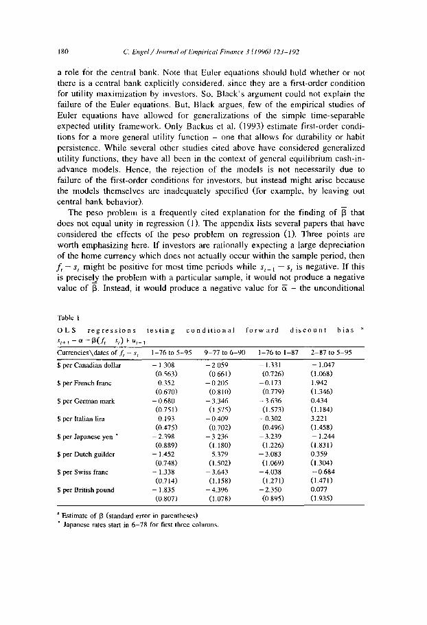
180 C. E n g e l / J o u r n a l ¢?f Emp i r i ca l F inance 3 (1996) 1 2 3 - 1 9 2

a role for the central bank. Note that Euler equat ions should hold whether or not

there is a central bank expl ici t ly considered, since they are a f irst-order condi t ion for utility max imiza t ion by investors. So, B lack ' s a rgument could not expla in the

fai lure o f the Euler equations. But, Black argues, few of the empir ical studies of

Euler equat ions have a l lowed for general iza t ions o f the s imple t ime-separable expec ted utility f ramework . Only Backus et al. (1993) es t imate f irs t-order condi-

t ions for a more general utility funct ion - one that a l lows for durabil i ty or habit

persistence. Whi le several other studies ci ted above have considered genera l ized

utility functions, they have all been in the context o f general equi l ibr ium cash-in-

advance models . Hence , the reject ion o f the mode ls is not necessar i ly due to

failure o f the f irst-order condi t ions for investors, but instead might arise because

the mode l s themse lves are inadequate ly specif ied (for example , by leaving out

central bank behavior) .

The peso p rob lem is a f requent ly cited explanat ion for the f inding of ~ that

does not equal unity in regress ion (1). The appendix lists several papers that have

cons idered the effects o f the peso p rob lem on regression (1). Three points are

worth emphas iz ing here. I f investors are rat ional ly expect ing a large deprecia t ion

o f the home currency which does not actually occur within the sample period, then

f t - st might be posi t ive for most t ime per iods whi le s t + i - s t is negat ive. I f this is precise¿__y the problem with a part icular sample, it would not produce a negat ive

value o f 13. Instead, it wou ld produce a negat ive value for ~ - the uncondi t ional

Table 1

O L S r e g r e s s i o n s t e s t i n g

st+ I = et + f 3 ( f , - s t ) + ut+ 1

c o n d i t i o n a l f o r w a r d d i s c o u n t b i a s a

Currencies\dates of f t - sf 1-76 to 5-95 9-77 to 6-90 1-76 to 1-87 2-87 to 5-95

$ per Canadian dollar - 1.308 -2.059 - 1.331 - 1.047 (0.563) (0.661) (0.726) (1.068)

$ per French franc 0.352 - 0.205 - 0.173 1.942 (0.670) (0.810) (0.779) (1.346)

$ per German mark - 0.680 - 3.346 - 3.636 0.434 (0.751) (1.575) (I.573) (1.184)

$ per Italian lira 0.193 - 0.409 - 0.302 3.221 (0.475) (0.702) (0.496) (1.458)

$ per Japanese yen * - 2.398 - 3.236 - 3.239 - 1.244 (0.889) (1.180) (1.226) (1.831)

$ per Dutch guilder - 1.452 - 5.379 - 3.083 0.359 (0.748) (1.502) (1.069) (1.304)

$ per Swiss franc - 1.338 - 3.643 -4.038 -0.684 (0.714) (1.158) (1.271) (1.471)

$ per British pound - 1.835 -4.396 -2.350 0.077 (0.807) (1.078) (0.895) (1.935)

a Estimate of 13 (standard error in parentheses) * Japanese rates stasa in 6-78 for first three columns.

c. Engel / Journal o'[ Empirical Finance 3 (I 996) 123-192 181

expectation of s,+ L - - s t would appear biased within the sample. To produce a negative value for 13, it must be the case that when the expected depreciation is greater than average within the sample (so f t - s t is greater than its sample average), the actual appreciation is greater than its sample average (s,+ l - s r is more negative than its sample average.)

Second, in virtually all of the empirical studies cited above, the forward discount changes sign during the sample. Sometimes f, - s, is positive within the sample, indicating an expected depreciation, and sometimes it is negative, indicating an exp__ected appreciation. Hence, if the peso problem is to explain negative values of [3, it must explain the puzzle of why the unobserved event changes within the sample from being a large expected depreciation to a large expected appreciation.

Third, one might suspect the peso problem could not be an explanation for the finding of ~ < 1, since that finding occurs over such a wide variety of samples. As was noted earlier, the bias appears in studies for dozens of currencies relative to the dollar over virtually all sub-periods of the recent floating regime (post-1973). It also occurs for non-dollar floating rates, and it occurs for other time periods (such as the 1920s).

On the other hand, consider the estimates of Eq. (1) for one-month forward rates reported in Table 1, for eight currencies relative to the dollar. 38 For six of the eight exchange rates, ~ is significantly less than one over the entire sample of January 1976 to May 1995. Still, that result is less impressive than when the regression is run over McCal lum ' s (1994) time period of September 1977 to June 1990. In the latter time period, seven of the eight estimates of 13 are significantly less than one. Moreover, all of the estimates are less than zero, and they are all smaller than the estimates from the January 1976-May 1995 time period. So, while the case against unbiasedness is strong over the entire sample, it does not seem nearly as strong as it seems if one only were to look at McCal lum ' s sample.

If we split the sample into the period leading up to the Louvre accord, and the post-Louvre period, the coefficients appear to change dramatically. Such a split might be sensible, since the long swings in the dollar that appeared before the Louvre accord appear to have disappeared since. Here, Table 1 shows that pre-Louvre, all the estimates of 13 are negative, and seven of the eight are significantly less than one. Post-Louvre, no estimates of 13 are significantly less than one. In fact, five are positive.

This evidence suggests there is room for the peso problem to explain the apparent bias in estimates of 13. Still, one must be cautious about drawing

38 The data are end of month, average of bid and ask rates, obtained from Datastream. All data begin in January 1976, except for forward rates for the Japanese yen which begin in June 1978. All data go through June 1995. The exchange rates obtained are all in terms of British pounds, but were converted to dollar exchange rates.

182 C. Engel / Journal qf Empirical Finance 3 (1996) 123-192

conclusions too hastily from this exercise. One can always find evidence that is more or less favorable towards a hypothesis in selected sub-samples, so the true significance of the sample split in Table 1 is unclear. Moreover, even in the case most favorable to the unbiasedness hypothesis - the post-Louvre period - six of the eight point estimates of [3 are less than one.

Another tack has been to use data from surveys of foreign exchange traders to obtain an independent measure of agents ' exchange rate expectations. These data tend to show systematic bias in the reported expectations. Indeed, these expectations seem to be even more biased than the forward rate. 39 The appendix lists a large number of papers that have employed survey data.

If, based on the survey data, one is to adopt the stance that expectations are not rational, there are three important questions that must be answered.

First, if expectations are not rational, what are they? Perhaps there is no alternative model of expectations that can summarize how market participants actually forecast the future. If that is true, then economists will have severe problems understanding the economy, because expectations play a critical role in almost any economic transaction.

Second, why are agents acting irrationally? If agents are making forecasts that are systematically biased, it surely would be easy and nearly costless to correct those forecasts. Perhaps there are institutional constraints that lead to the forward rate bias. Take a simple example. A foreign exchange trader might be rewarded by his company for his batting average - the proportion of profitable trades he makes. If some currency changes are large but infrequent, the trader would bet against those changes. If many traders are following this practice, the forward rate would be biased. Even this example is not satisfactory, however. Why would the trader be rewarded for such a practice?

Third, even if the bias in some agents ' expectations impart a bias to the forward rate, why are there not rational agents who bet such large sums against the biased agents that the forward rate bias is el iminated? Perhaps the rational agents are much more risk averse than the biased agents, and therefore are unwilling to take the large uncovered positions necessary to drive the forward rate back to its unbiased level.

Another approach that has received only a bit of attention in the foreign exchange literature is the role of market frictions. He and Modest (1995) indicate that in many financial markets, frictions such as short-sale, borrowing, and solvency constraints, as well as transactions costs could substantially affect the Euler-equation estimates. In foreign exchange markets, all of these problems are much less severe than in many other financial markets. However, Baldwin (1990) argues that even very small transactions costs could lead to substantial forward

39 See, for example, Frankel and Froot (1987) and Froot and Frankel (1989).


rate bias. 40 Luttmer and Nishiotis (1995) incorporate transactions costs into calculations of the Hansen-Jagannathan bounds for models of international asset pricing. The introduction of transactions costs makes it much more plausible that excess returns on international bonds are consistent with standard measures of the intertemporal marginal rate of substitution in consumption.

Progress in any scientific field is usually made in small increments. While Hodr ick ' s (1987) conclusion - " W e do not yet have a model of expected returns that fits the da ta" - is equally applicable today, progress has been made. What we have learned since 1987 is that many simple explanations for the forward exchange rate bias do not work. We have ruled many things out, but have not yet settled on the ' t rue ' story.

Acknowledgements

I would like to thank Robert Hodrick, Nelson Mark, Richard Baillie and an anonymous referee for detailed comments on an earlier draft. I also thank Geert Bekaert, Fischer Black, Menzie Chinn, Jeffrey Frankel and participants at semi- nars at the Federal Reserve Board, the Federal Reserve Bank of Kansas City and New York University for useful comments, and Mike Hendrickson for excellent research assistance. Some of the work on this paper was completed while I was a Visiting Scholar at the Federal Reserve Bank of Kansas City and at the Board of Governors of the Federal Reserve System. The views expressed in this paper are my own and do not necessarily reflect those of the Federal Reserve. I also acknowledge assistance from the National Science Foundation, NSF grant # S B R - 932078.

Appendix A

Studies which have considered issues such as the peso problem, learning and shifts in regime include Bachman (1992), Bates (1994), Engel (1994b), Engel and Hamilton (1990), Evans and Lewis (1993), Evans and Lewis (1994), Goodhart et al. (1992), Kaminsky (1993), Kaminsky and Peruga (1991), and Lewis (1988c), Lewis (1989a), Lewis (1989b). Lewis (1994) and Evans (1995) survey this literature.

Survey data on exchange rate expectations has been employed by Cavaglia et al. (1993), Chinn and Frankel (1994), Frankel and Chinn (1993), Frankel and Froot (1987), Froot and Frankel (1989), Froot and Ito (1989), Ito (1990), Ito

4o See also Bossaerts and Hillion (1991), Goodhart and Taylor (1992), Hollifield and Uppal (1994) and Luttmer (1995).

184 c. Engel / Journal t~[ Empirical Finance 3 (1996) 123-192

(1994) , L iu and M a d d a l a (1992a) , L iu and M a d d a l a (1992b) , M a c D o n a l d (1990) ,

M a c D o n a l d (1992) , M a c D o n a l d and Tor r ance (1989) , M a c D o n a l d and T o r r a n c e

(1990) , Pope and Peel (1991) , T a y l o r ( 1 9 8 9 ) and W e e and S iong (1993) . Takag i

(1990) and Franke l and Rose (1994) su rvey this l i terature.

F ranke l and Froo t ( 1990a ) of fer a poss ib le exp lana t ion for the fo rward rate bias.

The mode l they presen t i n v o l v e s the in te rac t ion o f ' cha r t i s t s ' and ' f u n d a m e n t a -

l i s t s ' , and offers a theory o f the d y n a m i c s of e x c h a n g e rates and in teres t rates.

Empi r i ca l suppor t for the i r a p p r o a c h can be g l eaned f rom E i c h e n b a u m and E v a n s

(1994) and Gri l l i and R o u b i n i (1994) . Re la t ed papers inc lude A l l en and T a y l o r

(1990) , F ranke l and Froo t (1990b) , and Froo t and T h a l e r (1990) .

A s ign that marke t s m i g h t not be e f f ic ien t is i f t echn ica l t r ad ing rules are

prof i tab le . Sura ja ras and S w e e n e y ( 1 9 9 2 ) and L e v i c h and T h o m a s (1993) exp lo re

this poss ib i l i ty .

References

Alexander, C.O. and A. Johnson, 1992, Are foreign exchange markets really efficient?, Economics Letters 40, 449-453.

Allen, Helen and Mark P. Taylor, 1990, Chartists, noise and fundamentals in the London foreign exchange market, Economic Journal 100, supplement, 49-59.

Bachman, Daniel, 1992, The effect of political risk on the forward exchange bias: The case of elections, Journal of International Money and Finance 11, 208-219.

Backus, David, Allan Gregory and Chris Telmer, 1993, Accounting for forward rates in markets for foreign currency, Journal of Finance 48, 1887-1908.

Backus, David K., Silverio Foresi and Chris I. Telmer, 1994, The forward premium anomaly: Three examples in search of a solution (Stern School of Business, New York University, New York).

Baffes, John, 1994, Does comovement among exchange rates imply market inefficiency?, Economics Letters 44, 273-280.

Baillie, Richard T., 1989, Tests of rational expectations and market efficiency, Econometric Reviews 8, 151-186.

Baillie, Richard T. and Tim Bollerslev, 1989, Common stochastic trends in a system of exchange rates, Journal of Finance 44, 167-181.

Baillie, Richard T. and Tim Bollerslev, 1990, A multivariate generalized ARCH approach to modeling risk premia in forward foreign exchange markets, Journal of International Money and Finance 9, 309-324.

Baillie, Richard T. and Tim Bollerslev, 1994, The long memory of the forward premium, Journal of International Money and Finance 13, 565-571.

Baillie, Richard T., Tim Bollerslev and Hans Ole ,~E. Mikkelsen, 1996, Fractionally integrated generalized autoregressive conditional heteroskedasticiy, Journal of Econometrics, forthcoming.

Baillie, Richard T., Robert E. Lippens and Patrick C. McMahon, 1983, Testing rational expectations and efficiency in the foreign exchange market, Econometrica 51, 553-563.

Baldwin, Richard E., 1990, Reinterpreting the failure of foreign exchange market efficiency tests: Small transactions costs, big hysteresis bands, Working paper no. 3319 (NBER, Cambridge, MA).

Bandopadhyaya, Arindam, 1991, Speculative efficiency and risk premium in the market for foreign exchange: In search of the true specimen, Economics Letters 36, 299-304.

Barnhar't, Scott W. and Andrew C. Szakmary, 1991, Testing the unbiased forward rate hypothesis: Evidence on unit roots, co-integration and stochastic coefficients, Journal of Financial and Quantitative Analysis 26, 245-267.

C. Engel / Journal t~] Empirical Finance 3 (1996) 123-192 185

Bates, David, 1994, Dollar jump fears, 1984-1992, Working paper no. 94-2 (Wharton School, University of Pennsylvania, Philadelphia, PA) .

Bekaert, Geert, 1992, The time-variation of expected returns and volatility in foreign exchange markets, Journal of Business and Economics Statistics, forthcoming.

Bekaert, Geert, 1994a, The time variation of risk and return in foreign exchange markets: A general equilibrium perspective, Working paper no. 4818 (National Bureau of Economic Research, Cambridge, MA).

Bekaert, Geert, 1994b, Exchange rate volatility and deviations from unbiasedness in a cash-in-advance model, Journal of International Economics 36, 29-52.

Bekaert, Geert and Robert J. Hodrick, 1992, Characterizing predictable components in excess returns on equity and foreign exchange markets, Journal of Finance 47 ,467-509 .

Bekaert, Geert and Robert J. Hodrick, 1993, On biases in the measurement of foreign exchange risk premiums, Journal of International Money and Finance 12, 115-138.

Bekaert, Geert, Robert J. Hodrick and David A. Marshall, 1994, The implications of first-order risk aversion for asset market risk premiums, Working paper no. 4624 (National Bureau of Economic Research, Cambridge, MA).

Belongia, Michael T. and Mack Ott, 1989, The U.S. monetary policy regime, interest differentials and dollar exchange rate risk premia, Journal of International Money and Finance 8, 137-145.

Bilson, John F.O., 1981, The "speculative efficiency' hypothesis, Journal of Business 54, 435-452. Black, Fischer, 1994, Personal correspondence with the author. Black, Stanley W. and Michael K. Salemi, 1988, FIML estimation of the dollar-deutschemark risk

premium in a portfolio model, Journal of International Money and Finance 25, 250-270. Bollerslev, Tim, 1986, Generalized autoregressive conditional heteroskedasticity, Journal of Economet-

rics 31, 307-327. Bomhoff, Eduard and Kees G. Koedijk, 1988, Bilateral exchange rates and risk premia, Journal of

International Money and Finance 7, 205-220. Bossaerts, Peter and Pierre Hillion, 1991, Market microstructure effects of government intervention in

the foreign exchange market, Review of Financial Studies 4, 513-541. Boyer, R.A. and C.F. Adams, 1988, Forward premia and risk premia in a simple model of exchange

rate determination, Journal of Money, Credit and Banking 20, 633-644. Boyle, G., 1990, International interest rates, exchange rates, and the stochastic structure of supply,

Journal of Finance 45 ,655-671 . Breen, William, Lawrence Glosten and Ravi Jagannathan, 1989, Economic significance of predictable

variations in stock index returns, Review of Financial Studies 4, 1177-1189. Byers, J.D. and D.A. Peel, 1991, Some evidence on the efficiency of the sterling-dollar and

sterling-franc forward exchange rates in the interwar period, Economics Letters 35, 317-322. Campbell, John Y. and Richard H. Clarida, 1987, The term structure of Euromarket interest rates: An

empirical investigation, Journal of Monetary Economics 19, 25-44. Canova, Fabio, 1991, An empirical analysis of ex ante profits from forward speculation in foreign

exchange markets, Review of Economics and Statistics 73 ,489-496. Canova, Fabio and Takatoshi ito, 1991, The time-series properties of the risk premium in the

yen/dollar exchange market, Journal of Applied Econometrics 6, 125-142. Canova, Fabio and Jane Marrinan, 1993, Profits, risk and uncertainty in foreign exchange markets,

Journal of Monetary Economics 32, 259-286. Cavaglia, Stefano, Willem F.C. Verschoor and Christian C.P. Wolff, 1993, Further evidence on

exchange rate expectations, Journal of International Money and Finance 12, 78-98. Cheung, Yin-Wong, 1993, Exchange rate risk premiums, Journal of International Money and Finance

12, 182-194. Chinn, Menzie and Jeffrey A. Frankel, 1994, Patterns in exchange rate forecasts for twenty-five

currencies, Journal of Money, Credit and Banking 26, 759-769.

186 C. Engel / Journal t?[ Empirical Finance 3 (1996) 123-192

Choi, Seugmook and Benjamin J.C. Kim, 1991, Monetary policy regime changes and the risk premium in foreign exchange markets: A GARCH application, Economics Letters 37, 447-452.

Chrystal, K. Alec and Daniel L. Thornton, 1988, On the information content of spot and forward exchange rates, Journal of International Money and Finance 7, 321-330.

Clarida, Richard H. and Mark P. Taylor, 1993, The term structure of forward exchange risk premia and the forecastability of spot exchange rates: Correcting the errors, Working paper no. 4442 (NBER, Cambridge, MA).

Coleman, Mark, 1990, Cointegration-based tests of daily foreign exchange market efficiency, Eco- nomics Letters 32, 53-59.

Constantinides, George M. and Darrell Duffle, 1992, Asset pricing with heterogeneous consumers, Working paper (Graduate School of Business, University of Chicago, Chicago, IL).

Copeland, Laurence S., 1991, Cointegration tests of daily foreign exchange data, Oxford Bulletin of Economics and Statistics 53, 185-198.

Copeland, Laurence S., 1993, Efficiency of the forward market day by day and month by month, Applied Financial Economics 3, 79-87.

Cornell, Bradford, 1989, The impact of data errors on measurement of the foreign exchange risk premium, Journal of International Money and Finance 8, 147-157.

Crowder, William J., 1994, Foreign exchange market efficiency and common stochastic trends, Journal of International Money and Finance 13, 551-564.

Cumby, Robert E., 1988, Is it risk? Explaining deviations from uncovered interest panty, Journal of Monetary Economics 22, 279-299.

Cumby, Robert E. and John Huizinga, 1992, Investigating the correlation of unobserved expectations: Expected returns in equity and foreign exchange markets and other examples, Journal of Monetary Economics 30, 217-253.

Diebold, Francis X., Javier Gardeazabal and Kamil Yilmaz, 1994, On cointegration and exchange rate dynamics, Journal of Finance 49, 727-735.

Dornbusch, Rudiger, 1976, Expectations and exchange rate dynamics, Journal of Political Economy 84, 1161-1176.

Dumas, Bernard, 1993, Partial- vs. general-equilibrium models of the international capital market, Working paper no. 4446 (National Bureau of Economic Research, Cambridge, MA).

Dutton, John, 1993, Real and monetary shocks and risk premia in forward markets for foreign exchange, Journal of Money, Credit and Banking 25, 731-754.

Dwyer, Gerald P. and Myles S. Wallace, 1992, Cointegration and market efficiency, Journal of International Money and Finance 11, 318-327.

Eichenbaum, Martin and Charles L. Evans, 1994, Some empirical evidence on the effects of monetary policy shocks on exchange rates (Northwestern University, Evanston, IL).

Engel, Charles M., 1984, Testing for the absence of expected real profits from forward market speculation, Journal of International Economics 17, 309-324.

Engel, Charles M., 1992a, On the foreign exchange risk premium in a general equilibrium model, Journal of International Economics 32, 305-319.

Engel, Charles M., 1992b, The risk premium and the liquidity premium in foreign exchange markets, International Economic Review 33, 871-879.

Engel, Charles M., 1994a, Tests of CAPM on an international portfolio of bonds and stocks, In: Jeffrey A. Frankel, ed., The internationalization of equity markets (University of Chicago Press, Chicago, IL).

Engel, Charles M., 1994b, Can the Markov switching model forecast exchange rates?, Journal of International Economics 36, 151 - 165.

Engel, Charles M., 1995, A note on cointegration and international capital market efficiency, Journal of International Money and Finance, forthcoming.

Engle, Robert F. and Clive W.J. Granger, 1987, Cointegration and error correction: Representation, estimation and testing, Econometrica 55, 251-276.

C. Engel /Journal t~[Empirical Finance 3 (1996) 123-192 187

Engel, Charles M. and James D. Hamilton, 1990, Long swings in the dollar: Are they in the data and do markets know it?, American Economic Review 80, 689-713.

Engel, Charles M. and Anthony P. Rodrigues, 1989, Tests of international CAPM with time-varying covariances, Journal of Applied Econometrics 4, 119-138.

Engel, Charles M. and Anthony P. Rodrigues, 1993, Tests of mean-variance efficiency of international equity markets, Oxford Economic Papers 45, 403-421.

Epstein, Larry G. and Stanley E. Zin, 1990, 'First-order' risk aversion and the equity premium puzzle, Journal of Monetary Economics 26, 387-407.

Evans, Martin, D., 1995, Peso problems: Their theoretical and empirical implications, In: C.R. Rao, ed., Handbook of Statistics: Statistical Methods in Finance, forthcoming.

Evans, Martin D. and Karen Lewis, 1993, Trends in excess returns in currency and bond markets, European Economic Review 37, 1005-1019.

Evans, Martin D. and Karen K. Lewis, 1994, Do long term swings in the dollar affect estimates of the risk premia?, Review of Financial Studies, forthcoming.

Fama, Eugene, 1984, Forward and spot exchange rates, Journal of Monetary Economics 14, 319-338. Flood, Robert P. and Andrew K. Rose, 1994, Fixes: Of the forward discount puzzle, Working paper no.

4928 (National Bureau of Economic Research, Cambridge, MA). Frankel, Jeffrey A., 1979a, The diversifiability of exchange risk, Journal of International Economics 9,

379-393. Frankel, Jeffrey A., 1979b, On the mark: A theory of floating exchange rates based on real interest

differentials, American Economic Review 69, 601-622. Frankel, Jeffrey A., 1988, Recent estimates of time-variation in the conditional variance and in the

exchange risk premium, Journal of International Money and Finance 7, 115-125. Frankel, Jeffrey A. and Menzie Chinn, 1993, Exchange rate expectations and the risk premium: Tests

for a cross-section of 17 currencies, Review of International Economics I, 136-144. Frankel, Jeffrey A. and Kenneth A. Froot, 1987, Using survey data to test standard propositions

regarding exchange rate expectations, American Economic Review 77, 133-153. Frankel, Jeffrey A. and Kenneth A. Froot, 1990a, Chartists, fundamentalists, and the demand for

dollars, In: Anthony Courakis and Mark Taylor, eds., Private behavior and government policy in interdependent economies (Clarendon Press, Oxford).

Frankel, Jeffrey A. and Kenneth A. Froot, 1990b, Understanding the U.S. dollar in the eighties: The expectations of chartists and fundamentalists, Papers and Proceedings of the American Economic Association, 181 - 185.

Frankel, Jeffrey A. and Alan T. MacArthur, 1988, Political versus currency premia in international real interest differentials: A study of forward rates for 24 countries, European Economic Review 32, 1083-1121.

Frankel, Jeffrey A. and Andrew K. Rose, 1994, An empirical characterization of nominal exchange rates, In: Gene Grossman and Kenneth Rogoff, eds., The handbook of international economics (North-Holland, Amsterdam) forthcoming.

Fraser, Patricia and Mark P. Taylor, 1990, Modelling risk in the interwar foreign exchange market, Scottish Journal of Political Economy 37, 241-258.

Frenkel, Jacob A. and Assaf Razin, 1980, Stochastic prices and tests of efficiency of foreign exchange markets, Economics Letters 6, 165-170.

Froot, Kenneth A., 1990, Short rates and expected asset returns, Working paper no. 3247 (National Bureau of Economic Research, Cambridge, MA).

Froot, Kenneth A. and Jeffrey A. Frankel, 1989, Forward discount bias: Is it an exchange risk premium?, Quarterly Journal of Economics 104, 139-161.

Froot, Kenneth A. and Takatoshi Ito, 1989, On the consistency of short-run and long-run expectations, Journal of International Money and Finance 8, 487-510.

Froot, Kenneth and Richard H. Thaler, 1990, Anomalies: Foreign exchange, Journal of Economic Perspectives 4, no. 3, 179-192.

188 C Engel/Journal of Empirical Finance 3 (1996) 123-192

Giovannini, Alberto and Philippe Jorion, 1987, Interest rates and risk premia in the stock market and in the foreign exchange market, Journal of I ntemational Money and Finance 6, 107-124.

Giovannini, Alberto and Philippe Jorion, 1989, Time-variation of risk and return in the foreign exchange and stock markets, Journal of Finance 44, 307-326.

Gokey, Timothy C., 1994, What explains the risk premium in foreign exchange returns?, Journal of International Money and Finance 13, 729-738.

Goodhart, C.A.E.; P.C. McMahon and Y.L. Ngama, 1992, Does the forward premium/discount help to predict the future change in the exchange rate?, Scottish Journal of Political Economy 39, 129-140.

Goodhart, Charles A.E. and Mark P. Taylor, 1992, Why don't individuals speculate in forward foreign exchange?, Scottish Journal of Political Economy 39, 1-13.

Grilli, Vittorio and Nouriel Roubini, 1994, Liquidity and exchange rates: Puzzling evidence from the G-7 countries (Yale University, New Haven, CT).

Gul, Faruk, 1991, A theory of disappointment aversion, Econometrica 59, 667-686. Hakkio, Craig S., 1981, Expectations and the forward exchange rate, International Economic Review

22, 663-678. Hakkio, Craig S., 1986, Does the exchange rate follow a random walk? A Monte Carlo study of four

tests for a random walk, Journal of International Money and Finance 5, 221-229. Hakkio, Craig S. and Mark Rush, 1989, Market efficiency and cointegration: An application to the

sterling and deutschemark exchange markets, Journal of International Money and Finance 8, 75-88.

Hakkio, Craig S. and Anne Sibert, 1995, The foreign exchange risk premia: Is it real?, Journal of Money, Credit and Banking 27, 301-317.

Hamilton, James D., 1994, Time series analysis (Princeton University Press, Princeton, N J)). Hansen, Lars Peter, 1982, Large sample properties of generalized method of moments estimators,

Econometrica 50, 1029-1054. Hansen, Lars Peter and Robert J. Hodrick, 1983, Risk averse speculation in the forward foreign

exchange market: An econometric analysis of linear models, In: Jacob A. Frenkel, ed., Exchange rates and international macroeconomics (University of Chicago Press, Chicago, IL).

Hansen, Lars Peter and Ravi Jagannathan, 1991, Implications of security market data for models of dynamic economies, Journal of Political Economy 99, 225-262.

Hansen, Lars Peter and Kenneth Singleton, 1982, Generalized instrumental variables estimation of nonlinear rational expectations models, Econometrica 50, 1269-1286.

He, Hua and David Modest, 1995, Market frictions and consumption-based asset pricing, Journal of Political Economy 103, 94-117.

Hodrick, Robert J., 1987, The empirical evidence on the efficiency of forward and futures foreign exchange markets (Harwood, Char).

Hodrick, Robert J., 1989a, Risk, uncertainty and exchange rates, Journal of Monetary Economics 23, 433-459.

Hodrick, Robert J., 1989b, U.S. international capital flows: Perspectives from rational maximizing models, Carnegie-Rochester Conference Series on Public Policy 30, 231-288.

Hodrick, Robert J. and Sanjay Srivastava, 1984, An investigation of risk and return in forward foreign exchange, Journal of International Money and Finance 3, 1-29.

Hodrick, Robert J. and Sanjay Srivastava, 1986, The covariation of risk premiums and expected future spot rates, Journal of International Money and Finance 5 (supplement), 5-21.

Hollifield, Burton and Raman Uppal, 1994, A test of uncovered interest parity in segmented international commodity markets (Faculty of Commerce and Business Administration, University of British Columbia, Vancouver, BC).

Horvath, Michael T.K. and Mark W. Watson, 1994, Testing for cointegration when some of the cointegrating vectors are known, Technical working paper no, 171 (National Bureau of Economic Research, Cambridge, MA).


Huang, Roger D., 1989, An analysis of intertemporal pricing for forward exchange contracts, Journal of Finance 44, 183-194.

Huang, Roger D., 1990, Risk and parity in purchasing power, Journal of Money, Credit and Banking 22, 338-356.

lto, Takatoshi, 1988, Use of (time-domain) vector autoregressions to test uncovered interest panty, Review of Economics and Statistics 70, 296-305.

lto, Takatoshi, 1990, Foreign exchange rate expectations: Micro survey data, American Economic Review 80, 434-449.

Ito, Takatoshi, 1994, Short-run and long-run expectations of the yen/dollar exchange rate, Journal of the Japanese and International Economies 8, 119-143.

Ito, Takatoshi and Danny Quah, 1989, Hypothesis testing with restricted spectral density matrices, with an application to uncovered interest parity, International Economic Review 30, 203-215.

Johansen, Soren, 1988, Statistical analysis of cointegrating factors, Journal of Economic Dynamics and Control 12, 231-254.

Jung, Alexander C. and Volker Wieland, 1990, Forward rates and spot rates in the European Monetary System: Forward market efficiency, Weltwirtschaftliches Archiv 126, 615-629.

Kaminsky, Graciela, 1993, Is there a peso problem? Evidence from the dollar/pound exchange rate, 1976-1987, American Economic Review 83, 450-472.

Kaminsky, Graciela and Rodrigo Peruga, 1990, Can a time-varying risk premium explain excess returns in the forward market for foreign exchange?, Journal of International Economics 28, 47-70.

Kaminsky, Graciela and Rodrigo Peruga, 1991, Credibility crises: The dollar in the early 1980s, Journal of International Money and Finance 10, 170-192.

Kandel, Shmuel and Robert F. Stambaugh, 1991, Asset returns and intertemporal preferences, Journal of Monetary Economics 27, 39-71.

Kearney, Colm and Ronald MacDonald, 1991, Efficiency in the forward foreign exchange market: Weekly tests of the Australian/U.S. dollar exchange rate, January 1984-March 1987, Economic Record 67, 237-242.

Korajczyk, Robert A., 1985, The pricing of forward contracts for foreign exchange, Journal of Political Economy 93, 346-368.

Krugman, Paul, 1981, Consumption preferences, asset demands, and distribution effects in international financial markets, Working paper no. 651 (National Bureau of Economic Research, Cambridge, MA).

Kwiatowski, Denis, P.C.B. Phillips, Peter Schmidt and Yongcheol Shin, 1992, Testing the null hypothesis of stationarity against the alternative of a unit root: How sure are we that economic time series have a unit root?, Journal of Econometrics 54, 159-178.

Labadie, Pamela, 1986, Comparative dynamics and risk premia in an overlapping generations model, Review of Economic Studies 53, 139-152.

Levich, Richard M. and Lee R. Thomas III, 1993, The significance of technical trading-rule profits in the foreign exchange market: A bootstrap approach, Journal of International Money and Finance 12, 451-474.

Levine, Ross, 1989, The pricing of forward exchange rates, Journal of International Money and Finance 8, 163-179.

Levine, Ross, 1991, An empirical inquiry into the nature of the forward exchange rate bias, Journal of International Economics 30, 359-369.

Lewis, Karen K., 1988a, Testing the portfolio balance model: A multi-lateral approach, Journal of International Economics 24, 109-127.

Lewis, Karen K., 1988b, Inflation risk and asset market disturbances: The mean-variance model revisited, Journal of International Money and Finance 7, 273-288.

Lewis, Karen K., 1988c, The persistence of the 'peso problem' when policy is noisy, Journal of International Money and Finance 7, 1-1 I.

190 C. Engel / Journal t?f Empirical Finance 3 (1996) 123-192

Lewis, Karen K., 1989a, Changing beliefs and systematic rational forecast errors with evidence from foreign exchange, American Economic Review 79, 621-636.

Lewis, Karen K., 1989b, Can learning affect exchange-rate behavior?, Journal of Monetary Economics 23, 79-100.

Lewis, Karen K., 1990, The behavior of eurocurrency returns across different holding periods and regimes, Journal of Finance 45, 1211-1236.

Lewis, Karen, 1994, Puzzles in international financial markets, In: Gene Grossman and Kenneth Rogoff, eds., The handbook of international economics (North-Holland, Amsterdam) forthcoming.

Liu, Peter C. and G.S. Maddala, 1992a, Rationality of survey data and tests for market efficiency in the foreign exchange markets, Journal of International Money and Finance 1 I, 366-381.

Liu, Peter C. and G.S. Maddala, 1992b, Using survey data to test market efficiency in the foreign exchange markets, Empirical Economics 17, 303-332.

Lucas, Robert E., 1982, Interest rates and currency prices in a two-country world, Journal of Monetary Economics 10, 335-360.

Luttmer, Erzo, 1995, Asset pricing in economies with friction, Working paper no. 151 (Kellogg Graduate School of Management, Northwestern University, Evanston, IL).

Luttmer, Erzo, and George Nishiotis, 1995, Joint restrictions on preferences with non-traded goods and partially integrated financial markets (Kellogg Graduate School of Management, Northwestern University, Evanston, IL).

Lyons, Richard K., 1988, Tests of the foreign exchange risk premium using the expected second moments implied by option pricing, Journal of International Money and Finance 7, 91-108.

MacDonald, Ronald, 1990, Are foreign exchange market forecasters "rational'? Some survey-based tests, The Manchester School of Economics and Social Studies 58, 229-241.

MacDonald, Ronald, 1992, Exchange rate survey data: A disaggregated G-7 approach, The Manchester School of Economics and Social Studies 60, 147-162.

MacDonald, Ronald and Mark P. Taylor, 1989, Foreign exchange market efficiency and cointegration: Some evidence from the recent float, Economics Letters 29, 63-68.

MacDonald, Ronald and Mark P. Taylor, 1990, The term structure of forward foreign exchange premia: The inter-war experience, The Manchester School of Economics and Social Studies 58, 54-65.

MacDonald, Ronald and Mark P. Taylor, 1991, Risk, efficiency and speculation in the 1920s foreign exchange market: An overlapping data analysis, Weltwirtschaftliches Archiv 127, 500-523.

MacDonald, Ronald and Thomas S. Torrance, 1989, Some survey-based tests of uncovered interest parity, In: Ronald MacDonald and Mark P. Taylor, eds., Exchange rates and open economy macroeconomics (Blackwell, Oxford).

MacDonald, Ronald and Thomas S. Torrance, 1990, Expectations formation and risk in four foreign exchange markets, Oxford Economic Papers 42, 544-561.

Macklem, R. Tiff, 1991, Forward exchange rates in artificial economies, Journal of International Money and Finance 10, 365-391.

Mark, Nelson, 1985, On time varying risk premia in the foreign exchange market: An econometric analysis, Journal of Monetary Economics 16, 3-18.

Mark, Nelson, 1988, Time varying betas and risk premia in the pricing of forward foreign exchange contracts, Journal of Financial Economics 22, 335-354.

Mark, Nelson, Yangru Wu and Weike Hai, 1993, Understanding spot and forward exchange rate regressions (Ohio State University, Columbus, OH).

Marston, Richard C., 1993, Interest differentials under fixed and flexible exchange rates: The effects of capital controls and exchange risk, In: Michael D. Bordo and Barry Eichengreen, eds., A retrospective on the Bretton Woods system: Lessons for international monetary reform (University of Chicago Press, Chicago, IL).

Marston, Richard C., 1994, Tests of three parity conditions: Distinguishing risk premia and systematic forecast errors, Working paper no. 4923 (National Bureau of Economic Research, Cambridge, MA).


Mayfield, E. Scott and Robert G. Murphy, 1992, Interest rate parity and the exchange risk premium: Evidence from panel data, Economics Letters 40, 319-324.

McCallum, Bennett T., 1994, A reconsideration of the uncovered interest parity relationship, Journal of Monetary Economics 33, 105-132.

McCulloch, J. Huston, 1975, Operational aspects of the Siegel paradox, Quarterly Journal of Eco- nomics 89, 170-172.

McCurdy, Thomas H. and leuan Morgan, 1991, Tests for a systematic component in deviations from uncovered interest parity, Review of Economic Studies 58, 587-602.

McFarland, James W., Patrick C. McMahon, and Yerima Ngama, 1994, Forward exchange rates and expectations during the 1920s: A re-examination of the evidence, Journal of International Finance 13,627-636.

Mehra, Rajnish and Edward C. Prescott, 1985, The equity premium: A puzzle, Journal of Monetary Economics 15, 145-162.

Modjtahedi, Bagher, 1991, Multiple maturities and time-varying risk premia in forward exchange markets: An econometric analysis, Journal of International Economics 30, 69-86.

Ngama, Yerima C., 1992, Testing the efficiency of thin forward foreign exchange markets: An application of instrumental variable multiple regression with integrated, I(1), variables, Manchester School of Economic and Social Studies 60, 169-180.

Nijman, Theo, Franz C. Palm and Christian C.P. Wolff, 1993, Premia in forward foreign exchange as unobserved components: A note, Journal of Business and Economic Statistics 11, 361-365.

Phillips, Peter C.B. and Bruce E, Hansen, 1990, Statistical inference in instrumental variables regression with 1(1) processes, Review of Economic Studies 57, 99-125.

Pittis, Nikitas, 1992, Causes of the forward bias: Non-rational expectations versus risk premia, Applied Economics 24, 317-325.

Pope, Peter F. and David A. Peel, 1991, Forward foreign exchange rates and risk premia: A reappraisal, Journal of International Money and Finance 10, 443-456.

Reitz, Thomas A., 1988, The equity risk premium: a solution, Journal of Monetary Economics 22, 117-131.

Romer, David, 1995, Advanced macroeconomics (McGraw-Hill, New York). Sephton, Peter S. and Hans K. Larsen, 1991, Tests of exchange market efficiency: Fragile evidence

from cointegration tests, Journal of International Money and Finance 10, 561-570. Sibert, Anne, 1989, The risk premium in the foreign exchange market, Journal of Money, Credit and

Banking 21, 49-65. Sibert, Anne, 1992, Can unconventional preferences explain risk premia in the foreign exchange

market?, Working paper (Department of Economics, University of Kansas, Lawrence, KS). Smith, William T., 1991, Forward exchange rates in general equilibrium, Journal of International

Money and Finance 10, 497-511. Sosvilla-Rivero, Simon and Young B. Park, 1992, Further tests on the forward exchange unbiasedness

hypothesis, Economics Letters 40, 325-331. Stock, James H. and Mark W. Watson, 1993, A simple estimator of cointegrating vectors in higher

order integrated systems, Econometrica 61,783-820. Stulz, Rene, 1994, International portfolio choice and asset pricing: An integrative survey, Working

paper no. 4645 (NBER, Cambridge, MA). Surajaras, Patchara and Richard J. Sweeney, 1992, Profit-making speculation in foreign exchange

markets (Westview Press Press, Boulder, CO). Svensson, Lars E.O., 1985, Currency prices, terms of trade and interest rates: A general equilibrium

asset-pricing cash-in-advance approach, Journal of International Economics 18, 17-41. Takagi, Shinji, 1990, Exchange rate expectations: A survey of survey studies, IMF Staff Papers 38,

156-183. Taylor, Mark P., 1988, A DYMIMIC model of forward foreign exchange risk, with estimates for three

major exchange rates, Manchester School of Economics and Social Studies 56, 55-68.

192 C. Engel / Journal t?/Empirical Finance 3 (1996) 123-192

Taylor, Mark P., 1989, Expectations, risk and uncertainty in the foreign exchange market: Some results based on survey data, Manchester School of Economics and Social Studies 57, 142-153.

Tesar, Linda L. and lngrid M. Werner, 1994, International equity transactions and U.S. portfolio choice, in: Jeffrey A. Frankel, ed., The internationalization of equity markets (Chicago University Press, Chicago, IL).

Thomas, S.H. and M.R. Wickens, 1993, An international CAPM for bonds and equities, Journal of International Money and Finance 12, 390-412.

Tronzano, Marco, 1992, Efficiency in German and Japanese foreign exchange markets: Evidence from cointegration techniques, Weltwirtschaftliches Archiv 128, 1-20.

Wee Beng, Gan and Wong Keng Siong, 1993, Exchange rate expectations and risk premium in the Singapore/U.S. dollar exchange rate: Evidence from survey data, Applied Financial Economics 3, 365-373.

journal of empirical finance the forward discount … · portfolio-balance models of risk premiums....

Documents