A global construction of homogeneous planar STIT tessellations

Joseph Mecke, Friedrich-Schiller-Universität Jena,

Werner Nagel, Friedrich-Schiller-Universität Jena,

Viola Weiß, Fachhochschule Jena

AbstractHomogeneous (stationary) random tessellations of the Euclidean plane are constructedwhich have the characteristic property to be stable with respect to iteration (or nesting),STIT for short. A new approach is presented that describes the tessellation in the wholeplane. So far, it was only known how to construct those tessellations within boundedwindows.

Key words:stochastic geometry; random tessellation; Poisson point processes; itera-tion/nesting of tessellations; stability of distributions

AMS subject classification:60D05, 52A22

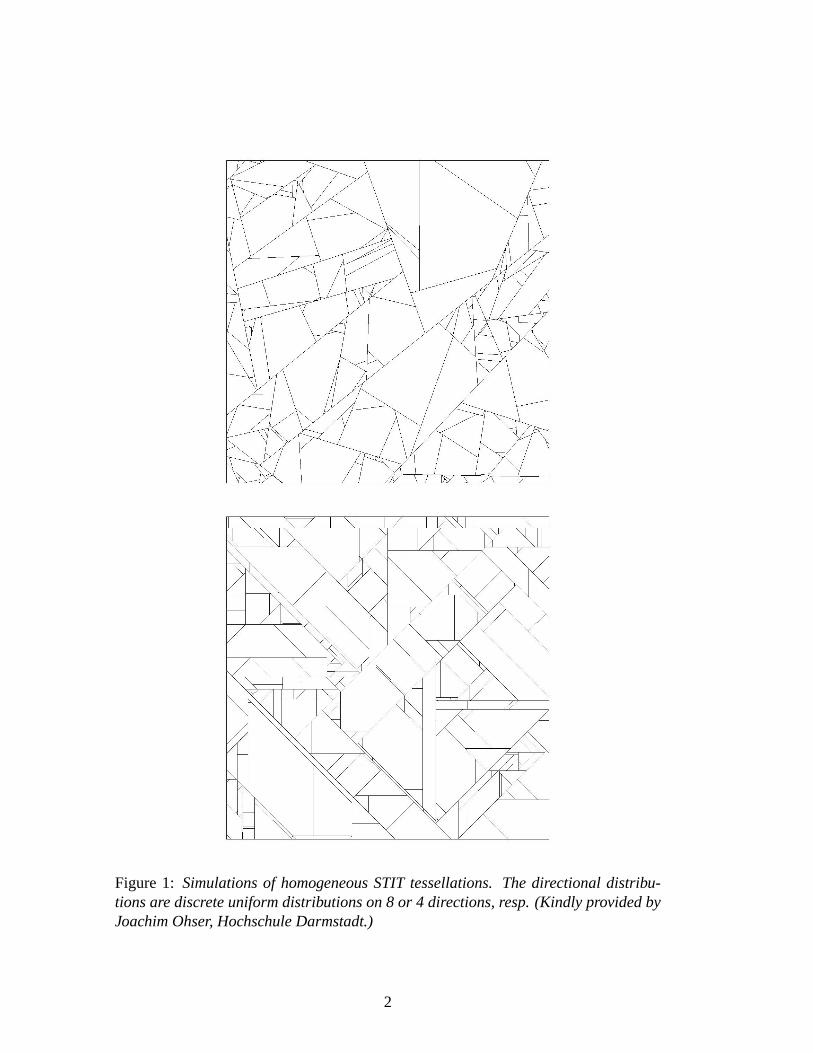
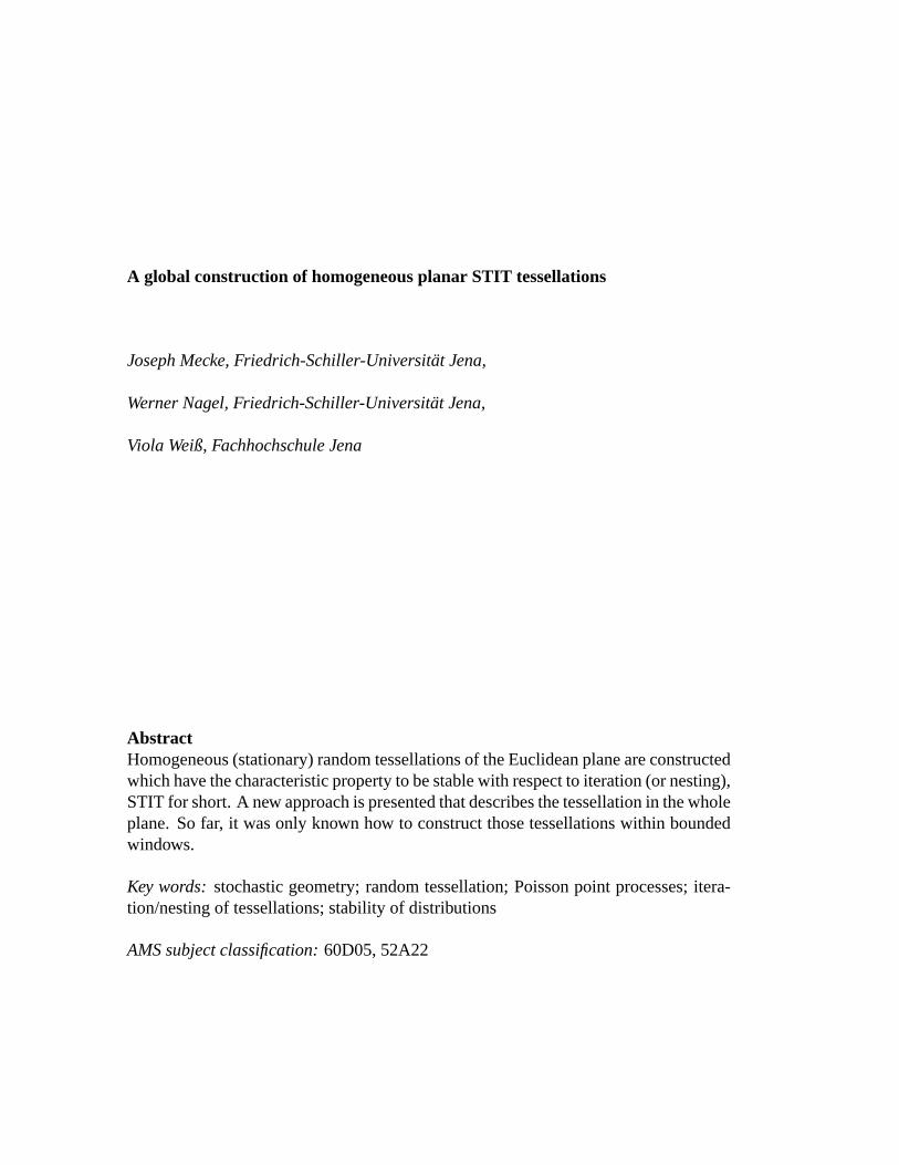
Figure 1: Simulations of homogeneous STIT tessellations. The directional distribu-tions are discrete uniform distributions on 8 or 4 directions, resp. (Kindly provided byJoachim Ohser, Hochschule Darmstadt.)

2

Figure 2:Simulations of homogeneous STIT tessellations. The directional distributionsare: Horizontal and vertical with 5/12 and the other two directions with 1/12 each(top), and directional distribution with density|cosα|/2 (bottom). (Kindly providedby Joachim Ohser, Hochschule Darmstadt.)

3

1 Introduction

In an earlier paper [7] a new type of random tessellations was introduced, the so-calledSTIT tessellations. This name indicates that a characteristic feature is their stochasticstability with respect to the operation iteration (or nesting) of tessellations. The exis-tence and a uniqueness result were already shown and a geometric construction wasdescribed that can be carried out in any bounded window. But it was not clear how toextend the construction to the whole infinite plane or space.In the present paper an alternative construction of the planar STIT tessellations is de-veloped, and this construction is not restricted to a window. Basically, the constructionis given by a deterministic map of a Poisson point processΠ on [0,π)×R× (0,∞),whereR denotes the set of real numbers. The points are interpreted as marked linesin the plane where the mark indicates the time of birth of the line. Thus, for any timet > 0 the set of all lines that are already born, forms a tessellation. The key idea is toconsider theo-cells, i.e. the cells containing the origin, as a process depending on thetime t. This sequence ofo-cells is monotonically decreasing. Since they are filling thewhole plane they give rise to a non-homogeneous (i.e. spatially non-stationary) tessel-lation Ψt where the cells are the set differences in the descending sequence ofo-cells.In a final step, the cells of the tessellationΨt are subdivided by an iteration/nesting ofa tessellation according to the above mentioned ’old’ construction in [7] for boundedwindows.A random tessellation in the plane can be described as a random ensemble of non-overlapping compact convex polygons – the cells – that fill the plane. Equivalently, itcan be considered as the random closed set – RACS for short – of all the boundariesof the cells. We will deliberately make use of both the definitions.In order to prove that the new construction indeed yields a homogeneous STIT tessel-lation its capacity functional is calculated and it is shown that it coincides with thatone which was given in [7].In the appendix we recall the definitions of iteration and of STIT.

2 The construction

The construction starts with an auxiliary spatial-temporal line process in the plane.The generated sequences ofo-cells is then used as the ’rough material’. Finally, thisensemble of convex polygons is divided further by random chords. This last step canalso be understood as a generalized iteration of tessellations.

2.1 A birth process for lines in the plane

In the Euclidean planeR2 we denote a line byg(α, p) = {(x,y) ∈ R2 : x cosα +y sinα = p}, (α, p) ∈ [0,π)×R, i.e. the line with the signed distancep ∈ R fromthe origin and the normal directionα ∈ [0,π) w.r.t. the abscissa axis.

4

The starting point is a Poisson point processΠ on the space[0,π)×R× (0,∞) withthe intensity measure

Λ = ϑ × `× `+ (1)

whereϑ is a probability measure that is not concentrated on a single point, i.e.ϑ({α})<1 for all α ∈ [0,π), ` is the Lebesgue measure onR, and`+ is its restriction to(0,∞),i.e. `+(·) = `(·∩ (0,∞)).To point(α, p, t) ∈ [0,π)×R× (0,∞) that belongs toΠ there corresponds the birth ofthe lineg(α, p) at timet.For t > 0 define

Γt = {g(α, p) : (α, p,s) ∈Π, s< t}. (2)

This is a homogeneous (spatially stationary, i.e. its distribution is invariant w.r.t. trans-lations in the plane) line process with directional distributionϑ and length intensity(mean total line length per unit area)LA(Γt) = t. Thus we have a stochastic process(Γt)t>0 on the space of line ensembles. The definition yields

Γt1 ⊆ Γt2 for t1 < t2. (3)

Furthermore, due to the properties of Poisson processΠ, the line processesΓt andΓt2 \Γt1 are independent ift ≤ t1 < t2.

2.2 The process of cells that contain the origin

For all t > 0 the Poisson line processΓt is a.s. (almost surely) not empty. Since itis assumed that the directional distributionϑ is not concentrated in a single point,Γt

a.s. generates a tessellation with a compact convex polygonZt that contains the origino in its interior. This polygon will be referred to as theo-cell of Γt . This yields thestochastic process(Zt)t>0. In the following, several of the assertions hold a.s. even ifwe do not indicate this everywhere.The isotony (3) implies

Zt1 ⊇ Zt2 for t1 < t2. (4)

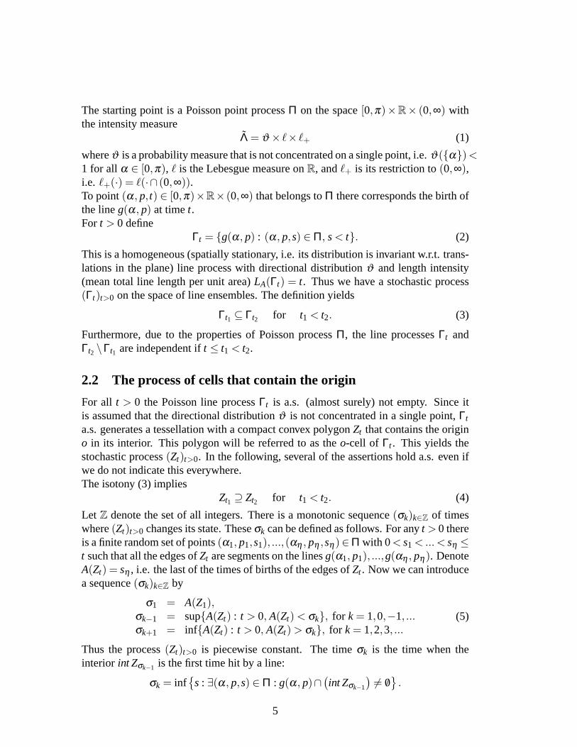
Let Z denote the set of all integers. There is a monotonic sequence(σk)k∈Z of timeswhere(Zt)t>0 changes its state. Theseσk can be defined as follows. For anyt > 0 thereis a finite random set of points(α1, p1,s1), ...,(αη , pη ,sη)∈Π with 0< s1 < ... < sη ≤t such that all the edges ofZt are segments on the linesg(α1, p1), ...,g(αη , pη). DenoteA(Zt) = sη , i.e. the last of the times of births of the edges ofZt . Now we can introducea sequence(σk)k∈Z by

σ1 = A(Z1),σk−1 = sup{A(Zt) : t > 0, A(Zt) < σk}, for k = 1,0,−1, ...σk+1 = inf{A(Zt) : t > 0, A(Zt) > σk}, for k = 1,2,3, ...

(5)

Thus the process(Zt)t>0 is piecewise constant. The timeσk is the time when theinterior int Zσk−1 is the first time hit by a line:

σk = inf{

s : ∃(α, p,s) ∈Π : g(α, p)∩(int Zσk−1

)6= /0

}.

5

Since for anyt > 0 we haveA(Zt)≤ t we obtain limk→−∞ σk = 0. On the other hand,limk→∞ σk = ∞ since for allt > 0

P(∃(α, p,s) ∈Π : s≥ t, g(α, p)∩ (int Zt) 6= /0) = 1.

It is crucial for the construction that the process of theo-cells fills the whole plane.

Lemma 1 ⋃k∈Z

Zσk = R2 a.s. (6)

Proof: Forx ∈ R2 and t > 0 denote byBx the circle of radius 1 and centerx andby (α1, p1,s1), ...,(αξ , pξ ,sξ ) ∈ Π the finite set with 0< s1 < ... < sξ ≤ t such that{g(α1, p1), ...,g(αξ , pξ )} is the set of all lines inΓt that intersect the setconv(Bx∪{o}), i.e. the convex hull ofBx and the origin. Thenx∈ int Zσk for all σk < s1. Thus

P(∃k∈ Z : Bx ⊂ Zσk) = 1.

With (4) and a coverage ofR2 by circlesBx, x from a countable set, the proof can becompleted. �On the other hand one can show that

⋂k∈Z Zσk = {o}.

2.3 A preliminary tessellation ofR2

Foru > 0 we define a tessellationΨu that is derived from the sequence(Zσk)k∈Z usingonly thoseZσk with σk ≤ u. The cells ofΨu are

Zu and Zσk−1 \Zσk, σk < u, (7)

whereB denotes the topological closure of a setB⊂ R2. All these cells are compact,convex and have a pairwise disjoint interior. Since, according to (5),Zσk = Zσk−1 ∩g(α, p)+1 with (α, p,σk) ∈ Π andg(α, p)+1 the closed half-plane that contains theorigin and is generated by the lineg(α, p). Due to (6) the cells fill the plane, i.e.

Zu∪⋃

σk<u

Zσk−1 \Zσk = R2.

The random tessellationΨu is non-homogeneous (spatially non-stationary). Intu-itively, the older cells ofΨu with σk−1, σk close to the time 0 (the moment of the’Big Bang’) are very far from the origino∈ R2 and they are stochastically larger thanthe younger ones. Also(Ψu)u>0 is a process of tessellations.

6

2.4 The final steps of the construction

Foru> 0 the random tessellationΦu is now constructed on the basis ofΨu. Sequencesof additional chords are nested into the cells ofΨu. In each of the cells the nestedtessellation is equivalent to that one which is given in [7] for bounded windows. Werecall this here briefly and adapt it to the present situation.Assign to each cellZσk−1 \Zσk, σk < u of Ψu, i.e. with the exception ofZu, a randomtessellationY(u−σk,Zσk−1 \Zσk) as it is defined in [7] and also described below.

2.4.1 Construction ofY(t,W) in a fixed window W

Let W be a compact convex polygon,t > 0 and the distributionϑ on [0,π) as it wasintroduced in 2.1. Denote by[W] the set of all linesg with g∩W 6= /0 and

Λ([W]) = Λ({(α, p,s) ∈ [0,π)×R× (0,∞) : g(α, p) ∈ [W], 0 < s≤ 1}) .

Let {(τ j ,γ j)}, j = 1,2, ... be an i.i.d. sequence of pairs of independent random vari-ables. Theτ j are exponentially distributed with parameterΛ([W]) and theγ j are ran-dom lines with the distributionΛ([W])−1Λ(· ∩ [W]), i.e. they have the directionaldistributionϑ . The idea is the following. After the lifetimeτ1 the polygonW is di-vided by the random chordW∩ γ1 into the two closed polygonsW∩ γ+1 andW∩ γ−1

whereγ+1 andγ−1 denote the two closed half-planes generated byγ1. Then these twopolygons are treated separately, their lifetimes, that begin at timeτ1, areτ2 andτ3 re-spectively. At the end of their lifetimes appear(W∩ γ

−11 )∩ γ

+12 , (W∩ γ

−11 )∩ γ

−12 and

(W∩γ+11 )∩γ

+13 , (W∩γ

+11 )∩γ

−13 . Some of these intersections can also be empty. This

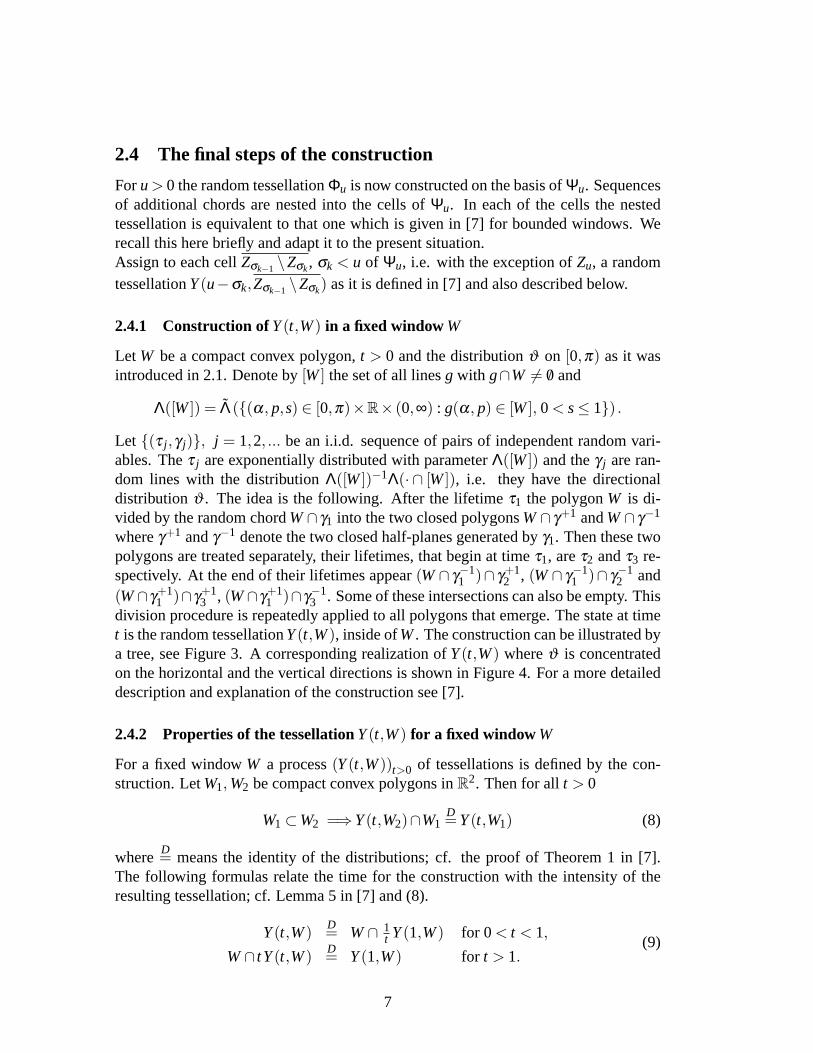
division procedure is repeatedly applied to all polygons that emerge. The state at timet is the random tessellationY(t,W), inside ofW. The construction can be illustrated bya tree, see Figure 3. A corresponding realization ofY(t,W) whereϑ is concentratedon the horizontal and the vertical directions is shown in Figure 4. For a more detaileddescription and explanation of the construction see [7].

2.4.2 Properties of the tessellationY(t,W) for a fixed window W

For a fixed windowW a process(Y(t,W))t>0 of tessellations is defined by the con-struction. LetW1, W2 be compact convex polygons inR2. Then for allt > 0

W1 ⊂W2 =⇒Y(t,W2)∩W1D= Y(t,W1) (8)

whereD= means the identity of the distributions; cf. the proof of Theorem 1 in [7].

The following formulas relate the time for the construction with the intensity of theresulting tessellation; cf. Lemma 5 in [7] and (8).

Y(t,W) D= W∩ 1t Y(1,W) for 0 < t < 1,

W∩ tY(t,W) D= Y(1,W) for t > 1.(9)

7

-0 t

Wτ1

γ1

W∩ γ+11

τ3γ3

W∩ γ−11

τ2 γ2

W∩ γ+11 ∩ γ

+13

τ7γ7

W∩ γ+11 ∩ γ

−13

τ6 γ6

W∩ γ−11 ∩ γ

+12

τ5

W∩ γ−11 ∩ γ

−12

τ4

...τ15

...τ14 γ14

...τ29

γ29

...τ28

...τ13

...τ12

...τ59

...τ58

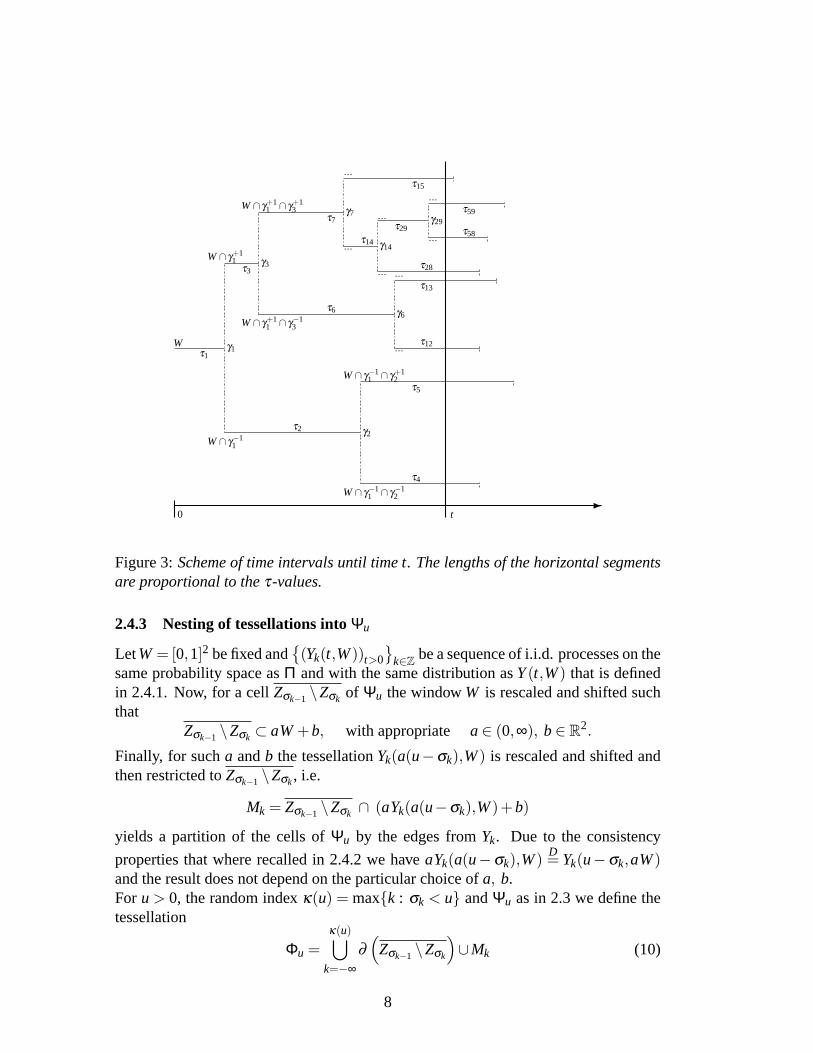
Figure 3:Scheme of time intervals until time t. The lengths of the horizontal segmentsare proportional to theτ-values.

2.4.3 Nesting of tessellations intoΨu

LetW = [0,1]2 be fixed and{(Yk(t,W))t>0

}k∈Z be a sequence of i.i.d. processes on the

same probability space asΠ and with the same distribution asY(t,W) that is definedin 2.4.1. Now, for a cellZσk−1 \Zσk of Ψu the windowW is rescaled and shifted suchthat

Zσk−1 \Zσk ⊂ aW+b, with appropriate a∈ (0,∞), b∈ R2.

Finally, for sucha andb the tessellationYk(a(u−σk),W) is rescaled and shifted andthen restricted toZσk−1 \Zσk, i.e.

Mk = Zσk−1 \Zσk ∩ (aYk(a(u−σk),W)+b)

yields a partition of the cells ofΨu by the edges fromYk. Due to the consistency

properties that where recalled in 2.4.2 we haveaYk(a(u−σk),W) D= Yk(u−σk,aW)and the result does not depend on the particular choice ofa, b.For u > 0, the random indexκ(u) = max{k : σk < u} andΨu as in 2.3 we define thetessellation

Φu =κ(u)⋃

k=−∞∂

(Zσk−1 \Zσk

)∪Mk (10)

8

γ1

γ3

γ2γ7

γ14

γ29

γ6

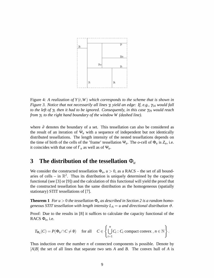
Figure 4: A realization of Y(t,W) which corresponds to the scheme that is shown inFigure 3. Notice that not necessarily all linesγi yield an edge: If, e.g.,γ14 would fallto the left ofγ1 then it had to be ignored. Consequently, in this caseγ29 would reachfrom γ1 to the right hand boundary of the window W (dashed line).

where∂ denotes the boundary of a set. This tessellation can also be considered asthe result of an iteration ofΨu with a sequence of independent but not identicallydistributed tessellations. The length intensity of the nested tessellations depends onthe time of birth of the cells of the ’frame’ tessellationΨu. Theo-cell of Φu is Zu, i.e.it coincides with that one ofΓu as well as ofΨu.

3 The distribution of the tessellationΦu

We consider the constructed tessellationΦu, u > 0, as a RACS – the set of all bound-aries of cells – inR2. Thus its distribution is uniquely determined by the capacityfunctional (see [3] or [9]) and the calculation of this functional will yield the proof thatthe constructed tessellation has the same distribution as the homogeneous (spatiallystationary) STIT tessellations of [7].

Theorem 1 For u> 0 the tessellationΦu as described in Section 2 is a random homo-geneous STIT tessellation with length intensity LA = u and directional distributionϑ .

Proof: Due to the results in [8] it suffices to calculate the capacity functional of theRACSΦu, i.e.

TΦu(C) = P(Φu∩C 6= /0) for all C∈

{n⋃

i=1

Ci : Ci compact convex, n∈ N

}.

Thus induction over the numbern of connected components is possible. Denote by[A|B] the set of all lines that separate two setsA and B. The convex hull ofA is

9

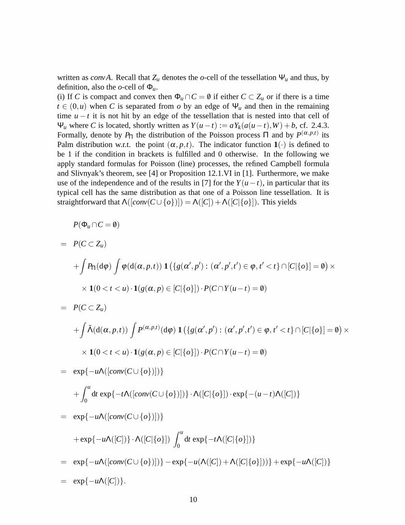
written asconvA. Recall thatZu denotes theo-cell of the tessellationΨu and thus, bydefinition, also theo-cell of Φu.(i) If C is compact and convex thenΦu∩C = /0 if eitherC⊂ Zu or if there is a timet ∈ (0,u) whenC is separated fromo by an edge ofΨu and then in the remainingtime u− t it is not hit by an edge of the tessellation that is nested into that cell ofΨu whereC is located, shortly written asY(u− t) := aYk(a(u− t),W)+ b, cf. 2.4.3.Formally, denote byPΠ the distribution of the Poisson processΠ and byP(α,p,t) itsPalm distribution w.r.t. the point(α, p, t). The indicator function1(·) is defined tobe 1 if the condition in brackets is fulfilled and 0 otherwise. In the following weapply standard formulas for Poisson (line) processes, the refined Campbell formulaand Slivnyak’s theorem, see [4] or Proposition 12.1.VI in [1]. Furthermore, we makeuse of the independence and of the results in [7] for theY(u− t), in particular that itstypical cell has the same distribution as that one of a Poisson line tessellation. It isstraightforward thatΛ([conv(C∪{o})]) = Λ([C])+Λ([C|{o}]). This yields

P(Φu∩C = /0)

= P(C⊂ Zu)

+∫

PΠ(dϕ)∫

ϕ(d(α, p, t)) 1({g(α ′, p′) : (α ′, p′, t ′) ∈ ϕ, t ′ < t}∩ [C|{o}] = /0

)×

× 1(0 < t < u) ·1(g(α, p) ∈ [C|{o}]) ·P(C∩Y(u− t) = /0)

= P(C⊂ Zu)

+∫

Λ(d(α, p, t))∫

P(α,p,t)(dϕ) 1({g(α ′, p′) : (α ′, p′, t ′) ∈ ϕ, t ′ < t}∩ [C|{o}] = /0

)×

× 1(0 < t < u) ·1(g(α, p) ∈ [C|{o}]) ·P(C∩Y(u− t) = /0)

= exp{−uΛ([conv(C∪{o})])}

+∫ u

0dt exp{−tΛ([conv(C∪{o})])} ·Λ([C|{o}]) ·exp{−(u− t)Λ([C])}

= exp{−uΛ([conv(C∪{o})])}

+exp{−uΛ([C])} ·Λ([C|{o}])∫ u

0dt exp{−tΛ([C|{o}])}

= exp{−uΛ([conv(C∪{o})])}−exp{−u(Λ([C])+Λ([C|{o}]))}+exp{−uΛ([C])}

= exp{−uΛ([C])}.

10

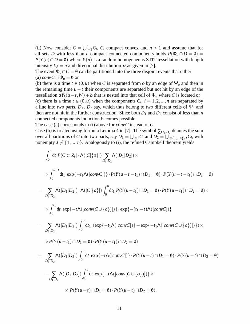
(ii) Now considerC =⋃n

i=1Ci , Ci compact convex andn > 1 and assume that forall setsD with less thann compact connected components holdsP(Φu∩D = /0) =P(Y(u)∩D = /0) whereY(u) is a random homogeneous STIT tessellation with lengthintensityLA = u and directional distributionϑ as given in [7].The eventΦu∩C = /0 can be partitioned into the three disjoint events that either(a)convC∩Φu = /0 or(b) there is a timet ∈ (0,u) whenC is separated fromo by an edge ofΨu and then inthe remaining timeu− t their components are separated but not hit by an edge of thetessellationaYk(u− t,W)+b that is nested into that cell ofΨu whereC is located or(c) there is a timet ∈ (0,u) when the componentsCi , i = 1,2, ...,n are separated bya line into two parts,D1, D2 say, which thus belong to two different cells ofΨu andthen are not hit in the further construction. Since bothD1 andD2 consist of less thannconnected components induction becomes possible.The case (a) corresponds to (i) above forconvCinstead ofC.Case (b) is treated using formula Lemma 4 in [7]. The symbol∑D1,D2

denotes the sumover all partitions ofC into two parts, sayD1 =

⋃i∈JCi andD2 =

⋃i∈{1,...n}\JCi , with

nonemptyJ 6= {1, ...,n}. Analogously to (i), the refined Campbell theorem yields∫ u

0dt P(C⊂ Zt) ·Λ([C|{o}]) ∑

D1,D2

Λ([D1|D2])×

×∫ u−t

0dt1 exp{−t1Λ([convC])} ·P(Y(u− t− t1)∩D1 = /0) ·P(Y(u− t− t1)∩D2 = /0)

= ∑D1,D2

Λ([D1|D2]) ·Λ([C|{o}])∫ u

0dt1 P(Y(u− t1)∩D1 = /0) ·P(Y(u− t1)∩D2 = /0)×

×∫ t1

0dt exp{−tΛ([conv(C∪{o})])} ·exp{−(t1− t)Λ([convC])}

= ∑D1,D2

Λ([D1|D2])∫ u

0dt1 (exp{−t1Λ([convC])}−exp{−t1Λ([conv(C∪{o})])})×

×P(Y(u− t1)∩D1 = /0) ·P(Y(u− t1)∩D2 = /0)

= ∑D1,D2

Λ([D1|D2])∫ u

0dt exp{−tΛ([convC])} ·P(Y(u− t)∩D1 = /0) ·P(Y(u− t)∩D2 = /0)

− ∑D1,D2

Λ([D1|D2])∫ u

0dt exp{−tΛ([conv(C∪{o})])}×

× P(Y(u− t)∩D1 = /0) ·P(Y(u− t)∩D2 = /0).

11

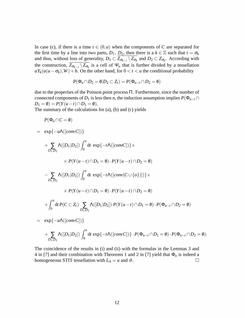
In case (c), if there is a timet ∈ (0,u) when the components ofC are separated forthe first time by a line into two parts,D1, D2, then there is ak ∈ Z such thatt = σk

and thus, without loss of generality,D1 ⊂ Zσk−1 \Zσk andD2 ⊂ Zσk. According withthe construction,Zσk−1 \Zσk is a cell of Ψu that is further divided by a tessellationaYk(a(u−σk),W)+b. On the other hand, for 0< t < u the conditional probability

P(Φu∩D2 = /0|D2 ⊂ Zt) = P(Φu−t ∩D2 = /0)

due to the properties of the Poisson point processΠ. Furthermore, since the number ofconnected components ofD1 is less thenn, the induction assumption impliesP(Φu−t∩D1 = /0) = P(Y(u− t)∩D1 = /0).The summary of the calculations for (a), (b) and (c) yields

P(Φu∩C = /0)

= exp{−uΛ([convC])}

+ ∑D1,D2

Λ([D1|D2])∫ u

0dt exp{−tΛ([convC])}×

× P(Y(u− t)∩D1 = /0) ·P(Y(u− t)∩D2 = /0)

− ∑D1,D2

Λ([D1|D2])∫ u

0dt exp{−tΛ([conv(C∪{o})])}×

× P(Y(u− t)∩D1 = /0) ·P(Y(u− t)∩D2 = /0)

+∫ u

0dt P(C⊂ Zt) ∑

D1,D2

Λ([D1|D2])·P(Y(u− t)∩D1 = /0) ·P(Φu−t ∩D2 = /0)

= exp{−uΛ([convC])}

+ ∑D1,D2

Λ([D1|D2])∫ u

0dt exp{−tΛ([convC])} ·P(Φu−t ∩D1 = /0) ·P(Φu−t ∩D2 = /0).

The coincidence of the results in (i) and (ii) with the formulas in the Lemmas 3 and4 in [7] and their combination with Theorems 1 and 2 in [7] yield thatΦu is indeed ahomogeneous STIT tessellation withLA = u andϑ . �

12

4 Outlook on a process of cell division that is homoge-neous in the plane

Our construction ofΦu suggests the following:To every cell ofΦu there can be assigned a time of birth at which it appears as one ofthe two parts in which a former cell is subdivided by a straight line generated byΠ orby the algorithms of nesting. All cells which have a time of birth smaller thans, s< u,form a tessellationΦs. In this way, we have constructed a stochastic process(Φs)0<s<u

on the time intervall(0,u), the states of which are tessellations of the plane.It can be shown thatΦs is distributed asΦs. This allows us to replace the notationΦs

by Φs. In particular, the random tessellationsΦs are STIT tessellations. Furthermore,they are homogeneous in the plane. But much more stronger, we guess that the processas a whole is spatially homogeneous. This can be expressed in an equivalent way:

Conjecture 1 For any0< s1 < ... < sn < u the distribution of the n-tuple[Φs1, ..,Φsn]is invariant under all shifts of the plane; n= 1,2,3, ...

Our process has the Markov property. It should be constructed on the whole positivetime axis.Summarizing the above considerations, we formulate:

Conjecture 2 Given a non-degenerate directional distributionϑ , there exists a sto-chastic process(Φt)t>0, the states of wich are tessellations of the Euclidean plane. Ithas the following properties.1. The process is homogeneous in the plane in the sense of Conjecture 1.2. For every t> 0 the random stateΦt is a homogeneous STIT tessellation with lengthintensity t and directional distributionϑ .3. For 0 < s< t < ∞ the net of edges ofΦs is a subset of the net of edges ofΦt .4. The process has the Markov property.5. Given 0 < s < t < ∞, the transition fromΦs to Φt can be regarded as an itera-tion procedure, whereΦs is the frame, and the cells ofΦs are filled according to thedistribution of Φt−s.

From property 2 we conclude thatt Φt is distributed asΦ1, i.e. up to a scaling factorall 1-dimensional distributions are the same.The process may be interpreted as a process of cell divisions. After a certain lifetimeevery cell is divided into two parts by a straight cut. The set of points in time in whicha cell division happens anywhere in the plane is dense in(0,∞) but countable.Some parts of Conjecture 2 are already proved implicitly in the preceding paragraphs.

13

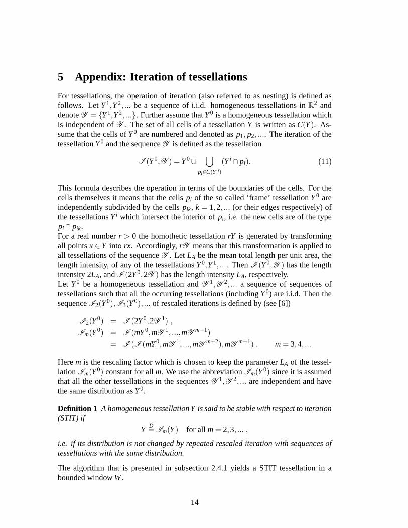
5 Appendix: Iteration of tessellations

For tessellations, the operation of iteration (also referred to as nesting) is defined asfollows. Let Y1,Y2, ... be a sequence of i.i.d. homogeneous tessellations inR2 anddenoteY = {Y1,Y2, ...}. Further assume thatY0 is a homogeneous tessellation whichis independent ofY . The set of all cells of a tessellationY is written asC(Y). As-sume that the cells ofY0 are numbered and denoted asp1, p2, .... The iteration of thetessellationY0 and the sequenceY is defined as the tessellation

I (Y0,Y ) = Y0∪⋃

pi∈C(Y0)

(Yi ∩ pi). (11)

This formula describes the operation in terms of the boundaries of the cells. For thecells themselves it means that the cellspi of the so called ’frame’ tessellationY0 areindependently subdivided by the cellspik, k = 1,2, ... (or their edges respectively) ofthe tessellationsYi which intersect the interior ofpi , i.e. the new cells are of the typepi ∩ pik.For a real numberr > 0 the homothetic tessellationrY is generated by transformingall pointsx∈Y into rx. Accordingly,rY means that this transformation is applied toall tessellations of the sequenceY . Let LA be the mean total length per unit area, thelength intensity, of any of the tessellationsY0,Y1, .... ThenI (Y0,Y ) has the lengthintensity 2LA, andI (2Y0,2Y ) has the length intensityLA, respectively.Let Y0 be a homogeneous tessellation andY 1,Y 2, ... a sequence of sequences oftessellations such that all the occurring tessellations (includingY0) are i.i.d. Then thesequenceI2(Y0),I3(Y0), ... of rescaled iterations is defined by (see [6])

I2(Y0) = I (2Y0,2Y 1) ,

Im(Y0) = I (mY0,mY 1, ...,mY m−1)= I (I (mY0,mY 1, ...,mY m−2),mY m−1) , m= 3,4, ...

Herem is the rescaling factor which is chosen to keep the parameterLA of the tessel-lationIm(Y0) constant for allm. We use the abbreviationIm(Y0) since it is assumedthat all the other tessellations in the sequencesY 1,Y 2, ... are independent and havethe same distribution asY0.

Definition 1 A homogeneous tessellation Y is said to be stable with respect to iteration(STIT) if

YD= Im(Y) for all m= 2,3, ... ,

i.e. if its distribution is not changed by repeated rescaled iteration with sequences oftessellations with the same distribution.

The algorithm that is presented in subsection 2.4.1 yields a STIT tessellation in abounded windowW.

14

A list of references concerning iteration was given in [6]. An approach to iterationwhich is more general than described above was developed in [2]. In the present paperthe step of the construction in paragraph 2.4.3 uses the idea of nesting of independentbut not identically distributed tessellations into a non-homogeneous ’frame’ tessella-tion.

References[1] DALEY, D. J. AND VERE-JONES, D. (1988).An introduction to the theory of point processes.

Springer Verlag, New York.

[2] M AIER, R., SCHMIDT, V. (2003). Stationary iterated tessellations.Adv. Appl. Prob. (SGSA)35,337–353.

[3] M ATHÉRON, G. (1975).Random sets and integral geometry.John Wiley & Sons, New York,London.

[4] M ECKE, J. (1967). Stationäre zufällige Maße auf lokalkompakten Abelschen Gruppen.Z.Wahrscheinlichkeitstheorie verw. Geb.9, 36–58.

[5] M ECKE, J. (1980). Palm methods for stationary random mosaics. InCombinatorial Principles inStochastic Geometry(ed. R.V. Ambartzumjan). Armenian Academy of Sciences Publ., Erevan,124–132.

[6] NAGEL, W. AND WEISS, V. (2003). Limits of sequences of stationary planar tessellations.Adv.Appl. Prob. (SGSA)35,123–138.

[7] NAGEL, W. AND WEISS, V. (2005). The crack tessellations – characterization of the stationaryrandom tessellations which are stable with respect to iteration.Adv. Appl. Prob. (SGSA)37,859–883.

[8] NORBERG, T. (1984). Convergence and existence of random set distributions.Ann. Prob.12,726–732.

[9] STOYAN , D., KENDALL , W. S. AND MECKE, J. (1995).Stochastic Geometry and its Applica-tions. 2nd edn. Wiley, Chichester.

15