jop reference handbook - jop: a tiny java processor … · jop reference handbook building embedded...
TRANSCRIPT
JOP Reference Handbook

JOP Reference HandbookBuilding Embedded Systems with a Java Processor
Martin Schoeberl
Copyright c© 2009 Martin Schoeberl
Martin SchoeberlStrausseng. 2-10/2/55A-1050 Vienna, Austria
Email: [email protected] the accompanying web site on http://www.jopdesign.com/ andthe JOP Wiki at http://www.jopwiki.com/
Published 2009 by CreateSpace,http://www.createspace.com/
All rights reserved. No part of this publication may be reproduced, stored in a retrieval system, ortransmitted in any form or by any means, electronic, mechanical, recording or otherwise, withoutthe prior written permission of Martin Schoeberl.
Library of Congress Cataloging-in-Publication Data
Schoeberl, Martin
JOP Reference Handbook: Building Embedded Systemswith a Java Processor / Martin SchoeberlIncludes bibliographical references and index.ISBN 978-1438239699
Manufactured in the United States of America.Typeset in 11pt Times by Martin Schoeberl
Foreword
This book is about JOP, the Java Optimized Processor. JOP is an implementation of theJava virtual machine (JVM) in hardware. The main implementation platform is a field-programmable gate array (FPGA). JOP began as a research project for a PhD thesis. In themean time, JOP has been used in several industrial applications and as a research platform.JOP is a time-predictable processor for hard real-time systems implemented in Java.
JOP is open-source under the GNU GPL and has a growing user base. This book iswritten for all of you who build this lively community. For a long time the PhD thesis,some research papers, and the web site have been the main documentation for JOP. A PhDthesis focus is on research results and implementation details are usually omitted. Thisbook complements the thesis and provides insight into the implementation of JOP and theaccompanying JVM. Furthermore, it gives you an idea how to build an embedded real-timesystem based on JOP.
V

Acknowledgements
Many users of JOP contributed to the design of JOP and to the tool chain. I also wantto thank the students at the Vienna University of Technology during the four years of thecourse “The JVM in Hardware” and the students from CBS, Copenhagen at an embed-ded systems course in Java for the interesting questions and discussions. Furthermore, thequestions and discussions in the Java processor mailing list provided valuable input for thedocumentation now available in form of this book. The following list of contributors to JOPis roughly in chronological order.
Ed Anuff wrote testmon.asm to perform a memory interface test and BlockGen.java to con-vert Altera .mif files to Xilinx memory blocks. Flavius Gruian wrote the initial version ofJOPizer to generate the .jop file from the application classes. JOPizer is based on the opensource library BCEL and is a substitute to the formerly used JavaCodeCompact from Sun.Peter Schrammel and Christof Pitter have implemented the first version of long bytecodes.Rasmus Pedersen based a class on very small information systems on JOP and invited my toco-teach this class in Copenhagen. During this time the first version of the WCET analysistool was developed by Rasmus. Rasmus has also implemented an Eclipse plugin for the JOPdesign flow. Alexander Dejaco and Peter Hilber have developed the I/O interface board forthe LEGO Mindstorms. Christof Pitter designed and implemented the chip-multiprocessor(CMP) version of JOP during his PhD thesis. Wolfgang Puffitsch first contribution to JOPwas the finalization of the floating point library SoftFloat. Wolfgang, now an active de-veloper of JOP, contributed several enhancements (e.g., exceptions, HW field access, datacache,...) and works towards real-time garbage collection for the CMP version of JOP.Alberto Andriotti contributed several JVM test cases. Stefan Hepp has implemented an op-timizer at bytecode level during his Bachelor thesis work. Benedikt Huber has redesignedthe WCET analysis tool for JOP during his Master’s thesis. Trevor Harmon, who imple-mented the WCET tool Volta for JOP during his PhD thesis, helped me with proofreadingof the handbook.
Furthermore, I would like to thank Walter Wilhelm from EEG for taking the risk to ac-cept a JOP based hardware for the Kippfahrleitung project at a very early developmentstage of JOP. The development of JOP has received funding from the Wiener Innova-tionsfoderprogram (Call IKT 2004) and from the EU project JEOPARD.

Contents
Foreword v
Acknowledgements vii
1 Introduction 11.1 A Quick Tour on JOP . . . . . . . . . . . . . . . . . . . . . . . . . . . . . 1
1.1.1 Building JOP and Running “Hello World” . . . . . . . . . . . . . . 11.1.2 The Design Structure . . . . . . . . . . . . . . . . . . . . . . . . . 2
1.2 A Short History . . . . . . . . . . . . . . . . . . . . . . . . . . . . . . . . 31.3 JOP Features . . . . . . . . . . . . . . . . . . . . . . . . . . . . . . . . . 41.4 Is JOP the Solution for Your Problem? . . . . . . . . . . . . . . . . . . . . 61.5 Outline of the Book . . . . . . . . . . . . . . . . . . . . . . . . . . . . . . 6
2 The Design Flow 92.1 Introduction . . . . . . . . . . . . . . . . . . . . . . . . . . . . . . . . . . 9
2.1.1 Tools . . . . . . . . . . . . . . . . . . . . . . . . . . . . . . . . . 92.1.2 Getting Started . . . . . . . . . . . . . . . . . . . . . . . . . . . . 102.1.3 Xilinx Spartan-3 Starter Kit . . . . . . . . . . . . . . . . . . . . . 11
2.2 Booting JOP — How Your Application Starts . . . . . . . . . . . . . . . . 122.2.1 FPGA Configuration . . . . . . . . . . . . . . . . . . . . . . . . . 122.2.2 Java Download . . . . . . . . . . . . . . . . . . . . . . . . . . . . 122.2.3 Combinations . . . . . . . . . . . . . . . . . . . . . . . . . . . . . 132.2.4 Stand Alone Configuration . . . . . . . . . . . . . . . . . . . . . . 14
2.3 The Design Flow . . . . . . . . . . . . . . . . . . . . . . . . . . . . . . . 152.3.1 Tools . . . . . . . . . . . . . . . . . . . . . . . . . . . . . . . . . 152.3.2 Targets . . . . . . . . . . . . . . . . . . . . . . . . . . . . . . . . 16
2.4 Eclipse . . . . . . . . . . . . . . . . . . . . . . . . . . . . . . . . . . . . . 182.5 Simulation . . . . . . . . . . . . . . . . . . . . . . . . . . . . . . . . . . . 19
2.5.1 JopSim Simulation . . . . . . . . . . . . . . . . . . . . . . . . . . 192.5.2 VHDL Simulation . . . . . . . . . . . . . . . . . . . . . . . . . . 20
X CONTENTS
2.6 Files Types You Might Encounter . . . . . . . . . . . . . . . . . . . . . . 212.7 Information on the Web . . . . . . . . . . . . . . . . . . . . . . . . . . . . 232.8 Porting JOP . . . . . . . . . . . . . . . . . . . . . . . . . . . . . . . . . . 23
2.8.1 Test Utilities . . . . . . . . . . . . . . . . . . . . . . . . . . . . . 232.9 Extending JOP . . . . . . . . . . . . . . . . . . . . . . . . . . . . . . . . 24
2.9.1 Native Methods . . . . . . . . . . . . . . . . . . . . . . . . . . . . 252.9.2 A new Peripheral Device . . . . . . . . . . . . . . . . . . . . . . . 252.9.3 A Customized Instruction . . . . . . . . . . . . . . . . . . . . . . 262.9.4 Dependencies and Configurations . . . . . . . . . . . . . . . . . . 27
2.10 Directory Structure . . . . . . . . . . . . . . . . . . . . . . . . . . . . . . 282.10.1 The Java Sources for JOP . . . . . . . . . . . . . . . . . . . . . . 30
2.11 The JOP Hello World Exercise . . . . . . . . . . . . . . . . . . . . . . . . 302.11.1 Manual build . . . . . . . . . . . . . . . . . . . . . . . . . . . . . 302.11.2 Using make . . . . . . . . . . . . . . . . . . . . . . . . . . . . . . 312.11.3 Change the Java Program . . . . . . . . . . . . . . . . . . . . . . . 312.11.4 Change the Microcode . . . . . . . . . . . . . . . . . . . . . . . . 312.11.5 Use a Different Target Board . . . . . . . . . . . . . . . . . . . . . 322.11.6 Compile a Different Java Application . . . . . . . . . . . . . . . . 322.11.7 Simulation . . . . . . . . . . . . . . . . . . . . . . . . . . . . . . 332.11.8 WCET Analysis . . . . . . . . . . . . . . . . . . . . . . . . . . . 33
3 Java and the Java Virtual Machine 353.1 Java . . . . . . . . . . . . . . . . . . . . . . . . . . . . . . . . . . . . . . 35
3.1.1 History . . . . . . . . . . . . . . . . . . . . . . . . . . . . . . . . 373.1.2 The Java Programming Language . . . . . . . . . . . . . . . . . . 38
3.2 The Java Virtual Machine . . . . . . . . . . . . . . . . . . . . . . . . . . . 393.2.1 Memory Areas . . . . . . . . . . . . . . . . . . . . . . . . . . . . 403.2.2 JVM Instruction Set . . . . . . . . . . . . . . . . . . . . . . . . . 403.2.3 Methods . . . . . . . . . . . . . . . . . . . . . . . . . . . . . . . 423.2.4 Implementation of the JVM . . . . . . . . . . . . . . . . . . . . . 43
3.3 Embedded Java . . . . . . . . . . . . . . . . . . . . . . . . . . . . . . . . 443.4 Summary . . . . . . . . . . . . . . . . . . . . . . . . . . . . . . . . . . . 45
4 Hardware Architecture 474.1 Overview of JOP . . . . . . . . . . . . . . . . . . . . . . . . . . . . . . . 474.2 Microcode . . . . . . . . . . . . . . . . . . . . . . . . . . . . . . . . . . . 49
4.2.1 Translation of Bytecodes to Microcode . . . . . . . . . . . . . . . 49
CONTENTS XI
4.2.2 Compact Microcode . . . . . . . . . . . . . . . . . . . . . . . . . 514.2.3 Instruction Set . . . . . . . . . . . . . . . . . . . . . . . . . . . . 524.2.4 Bytecode Example . . . . . . . . . . . . . . . . . . . . . . . . . . 534.2.5 Microcode Branches . . . . . . . . . . . . . . . . . . . . . . . . . 544.2.6 Flexible Implementation of Bytecodes . . . . . . . . . . . . . . . . 544.2.7 Summary . . . . . . . . . . . . . . . . . . . . . . . . . . . . . . . 55
4.3 The Processor Pipeline . . . . . . . . . . . . . . . . . . . . . . . . . . . . 554.3.1 Java Bytecode Fetch . . . . . . . . . . . . . . . . . . . . . . . . . 564.3.2 Microcode Instruction Fetch . . . . . . . . . . . . . . . . . . . . . 574.3.3 Decode and Address Generation . . . . . . . . . . . . . . . . . . . 594.3.4 Execute . . . . . . . . . . . . . . . . . . . . . . . . . . . . . . . . 604.3.5 Interrupt Logic . . . . . . . . . . . . . . . . . . . . . . . . . . . . 614.3.6 Summary . . . . . . . . . . . . . . . . . . . . . . . . . . . . . . . 62
4.4 The Stack Cache . . . . . . . . . . . . . . . . . . . . . . . . . . . . . . . 634.4.1 Java Computing Model . . . . . . . . . . . . . . . . . . . . . . . . 634.4.2 Access Patterns on the Java Stack . . . . . . . . . . . . . . . . . . 664.4.3 JVM Stack Access Revised . . . . . . . . . . . . . . . . . . . . . 674.4.4 A Two-Level Stack Cache . . . . . . . . . . . . . . . . . . . . . . 694.4.5 Summary . . . . . . . . . . . . . . . . . . . . . . . . . . . . . . . 72
4.5 The Method Cache . . . . . . . . . . . . . . . . . . . . . . . . . . . . . . 734.5.1 Method Cache Architecture . . . . . . . . . . . . . . . . . . . . . 734.5.2 WCET Analysis . . . . . . . . . . . . . . . . . . . . . . . . . . . 754.5.3 Caches Compared . . . . . . . . . . . . . . . . . . . . . . . . . . 774.5.4 Summary . . . . . . . . . . . . . . . . . . . . . . . . . . . . . . . 79
5 Runtime System 815.1 A Real-Time Profile for Embedded Java . . . . . . . . . . . . . . . . . . . 81
5.1.1 Application Structure . . . . . . . . . . . . . . . . . . . . . . . . . 825.1.2 Threads . . . . . . . . . . . . . . . . . . . . . . . . . . . . . . . . 825.1.3 Scheduling . . . . . . . . . . . . . . . . . . . . . . . . . . . . . . 835.1.4 Memory . . . . . . . . . . . . . . . . . . . . . . . . . . . . . . . . 835.1.5 Restrictions on Java . . . . . . . . . . . . . . . . . . . . . . . . . 865.1.6 Interaction of RtThread, the Scheduler, and the JVM . . . . . . . . 875.1.7 Implementation Results . . . . . . . . . . . . . . . . . . . . . . . 875.1.8 Summary . . . . . . . . . . . . . . . . . . . . . . . . . . . . . . . 89
5.2 A Profile for Safety Critical Java . . . . . . . . . . . . . . . . . . . . . . . 895.2.1 Introduction . . . . . . . . . . . . . . . . . . . . . . . . . . . . . . 89
XII CONTENTS
5.2.2 SCJ Level 1 . . . . . . . . . . . . . . . . . . . . . . . . . . . . . . 905.3 JVM Architecture . . . . . . . . . . . . . . . . . . . . . . . . . . . . . . . 94
5.3.1 Runtime Data Structures . . . . . . . . . . . . . . . . . . . . . . . 945.3.2 Class Initialization . . . . . . . . . . . . . . . . . . . . . . . . . . 985.3.3 Synchronization . . . . . . . . . . . . . . . . . . . . . . . . . . . 995.3.4 Booting the JVM . . . . . . . . . . . . . . . . . . . . . . . . . . . 100
6 Worst-Case Execution Time 1036.1 Microcode WCET Analysis . . . . . . . . . . . . . . . . . . . . . . . . . . 104
6.1.1 Microcode Path Analysis . . . . . . . . . . . . . . . . . . . . . . . 1046.1.2 Microcode Low-level Analysis . . . . . . . . . . . . . . . . . . . . 1056.1.3 Bytecode Independency . . . . . . . . . . . . . . . . . . . . . . . 1056.1.4 WCET of Bytecodes . . . . . . . . . . . . . . . . . . . . . . . . . 106
6.2 WCET Analysis of the Java Application . . . . . . . . . . . . . . . . . . . 1096.2.1 High-Level WCET Analysis . . . . . . . . . . . . . . . . . . . . . 1096.2.2 WCET Annotations . . . . . . . . . . . . . . . . . . . . . . . . . . 1106.2.3 ILP Formulation . . . . . . . . . . . . . . . . . . . . . . . . . . . 1116.2.4 An Example . . . . . . . . . . . . . . . . . . . . . . . . . . . . . 1136.2.5 Dynamic Method Dispatch . . . . . . . . . . . . . . . . . . . . . . 1156.2.6 Cache Analysis . . . . . . . . . . . . . . . . . . . . . . . . . . . . 1176.2.7 WCET Analyzer . . . . . . . . . . . . . . . . . . . . . . . . . . . 120
6.3 Evaluation . . . . . . . . . . . . . . . . . . . . . . . . . . . . . . . . . . . 1226.3.1 Benchmarks . . . . . . . . . . . . . . . . . . . . . . . . . . . . . . 1226.3.2 Analysis and Measurements . . . . . . . . . . . . . . . . . . . . . 124
6.4 Discussion . . . . . . . . . . . . . . . . . . . . . . . . . . . . . . . . . . . 1266.4.1 On Correctness of WCET Analysis . . . . . . . . . . . . . . . . . 1266.4.2 Is JOP the Only Target Architecture? . . . . . . . . . . . . . . . . 1266.4.3 Object-oriented Evaluation Examples . . . . . . . . . . . . . . . . 1276.4.4 WCET Analysis for Chip-multiprocessors . . . . . . . . . . . . . . 1276.4.5 Co-Development of Processor Architecture and WCET Analysis . . 1286.4.6 Further Paths to Explore . . . . . . . . . . . . . . . . . . . . . . . 128
6.5 Summary . . . . . . . . . . . . . . . . . . . . . . . . . . . . . . . . . . . 1286.6 Further Reading . . . . . . . . . . . . . . . . . . . . . . . . . . . . . . . . 129
6.6.1 WCET Analysis . . . . . . . . . . . . . . . . . . . . . . . . . . . 1296.6.2 WCET Analysis for Java . . . . . . . . . . . . . . . . . . . . . . . 1306.6.3 WCET Analysis for JOP . . . . . . . . . . . . . . . . . . . . . . . 131
CONTENTS XIII
7 Real-Time Garbage Collection 1337.1 Introduction . . . . . . . . . . . . . . . . . . . . . . . . . . . . . . . . . . 133
7.1.1 Incremental Collection . . . . . . . . . . . . . . . . . . . . . . . . 1357.1.2 Conservatism . . . . . . . . . . . . . . . . . . . . . . . . . . . . . 1357.1.3 Safety Critical Java . . . . . . . . . . . . . . . . . . . . . . . . . . 135
7.2 Scheduling of the Collector Thread . . . . . . . . . . . . . . . . . . . . . . 1367.2.1 An Example . . . . . . . . . . . . . . . . . . . . . . . . . . . . . 1377.2.2 Minimum Heap Size . . . . . . . . . . . . . . . . . . . . . . . . . 1397.2.3 Garbage Collection Period . . . . . . . . . . . . . . . . . . . . . . 143
7.3 SCJ Simplifications . . . . . . . . . . . . . . . . . . . . . . . . . . . . . . 1497.3.1 Simple Root Scanning . . . . . . . . . . . . . . . . . . . . . . . . 1497.3.2 Static Memory . . . . . . . . . . . . . . . . . . . . . . . . . . . . 150
7.4 Implementation . . . . . . . . . . . . . . . . . . . . . . . . . . . . . . . . 1517.4.1 Heap Layout . . . . . . . . . . . . . . . . . . . . . . . . . . . . . 1527.4.2 The Collector . . . . . . . . . . . . . . . . . . . . . . . . . . . . . 1537.4.3 The Mutator . . . . . . . . . . . . . . . . . . . . . . . . . . . . . 157
7.5 Evaluation . . . . . . . . . . . . . . . . . . . . . . . . . . . . . . . . . . . 1617.5.1 Scheduling Experiments . . . . . . . . . . . . . . . . . . . . . . . 1627.5.2 Measuring Release Jitter . . . . . . . . . . . . . . . . . . . . . . . 1677.5.3 Measurements . . . . . . . . . . . . . . . . . . . . . . . . . . . . 1697.5.4 Discussion . . . . . . . . . . . . . . . . . . . . . . . . . . . . . . 171
7.6 Analysis . . . . . . . . . . . . . . . . . . . . . . . . . . . . . . . . . . . . 1727.6.1 Worst Case Memory Consumption . . . . . . . . . . . . . . . . . . 1727.6.2 WCET of the Collector . . . . . . . . . . . . . . . . . . . . . . . . 172
7.7 Summary . . . . . . . . . . . . . . . . . . . . . . . . . . . . . . . . . . . 1737.8 Further Reading . . . . . . . . . . . . . . . . . . . . . . . . . . . . . . . . 173
8 Low-level I/O 1778.1 Hardware Objects . . . . . . . . . . . . . . . . . . . . . . . . . . . . . . . 177
8.1.1 An Example . . . . . . . . . . . . . . . . . . . . . . . . . . . . . 1778.1.2 Definition . . . . . . . . . . . . . . . . . . . . . . . . . . . . . . . 1798.1.3 Access Control . . . . . . . . . . . . . . . . . . . . . . . . . . . . 1808.1.4 Using Hardware Objects . . . . . . . . . . . . . . . . . . . . . . . 1828.1.5 Hardware Arrays . . . . . . . . . . . . . . . . . . . . . . . . . . . 1828.1.6 Garbage Collection . . . . . . . . . . . . . . . . . . . . . . . . . . 1828.1.7 Hardware Object Creation . . . . . . . . . . . . . . . . . . . . . . 1848.1.8 Board Configurations . . . . . . . . . . . . . . . . . . . . . . . . . 184
XIV CONTENTS
8.1.9 Implementation . . . . . . . . . . . . . . . . . . . . . . . . . . . . 1858.1.10 Legacy Code . . . . . . . . . . . . . . . . . . . . . . . . . . . . . 189
8.2 Interrupt Handlers . . . . . . . . . . . . . . . . . . . . . . . . . . . . . . . 1908.2.1 Synchronization . . . . . . . . . . . . . . . . . . . . . . . . . . . 1908.2.2 Interrupt Handler Registration . . . . . . . . . . . . . . . . . . . . 1938.2.3 Implementation . . . . . . . . . . . . . . . . . . . . . . . . . . . . 1938.2.4 An Example . . . . . . . . . . . . . . . . . . . . . . . . . . . . . 194
8.3 Standard Devices . . . . . . . . . . . . . . . . . . . . . . . . . . . . . . . 1958.3.1 The System Device . . . . . . . . . . . . . . . . . . . . . . . . . . 1958.3.2 The UART . . . . . . . . . . . . . . . . . . . . . . . . . . . . . . 195
9 The SimpCon Interconnect 1979.1 Introduction . . . . . . . . . . . . . . . . . . . . . . . . . . . . . . . . . . 197
9.1.1 Features . . . . . . . . . . . . . . . . . . . . . . . . . . . . . . . . 1989.1.2 Basic Read Transaction . . . . . . . . . . . . . . . . . . . . . . . . 1989.1.3 Basic Write Transaction . . . . . . . . . . . . . . . . . . . . . . . 199
9.2 SimpCon Signals . . . . . . . . . . . . . . . . . . . . . . . . . . . . . . . 1999.2.1 Master Signal Details . . . . . . . . . . . . . . . . . . . . . . . . . 1999.2.2 Slave Signal Details . . . . . . . . . . . . . . . . . . . . . . . . . 201
9.3 Slave Acknowledge . . . . . . . . . . . . . . . . . . . . . . . . . . . . . . 2029.4 Pipelining . . . . . . . . . . . . . . . . . . . . . . . . . . . . . . . . . . . 2049.5 Interconnect . . . . . . . . . . . . . . . . . . . . . . . . . . . . . . . . . . 2049.6 Examples . . . . . . . . . . . . . . . . . . . . . . . . . . . . . . . . . . . 206
9.6.1 I/O Port . . . . . . . . . . . . . . . . . . . . . . . . . . . . . . . . 2069.6.2 SRAM interface . . . . . . . . . . . . . . . . . . . . . . . . . . . 208
9.7 Available VHDL Files . . . . . . . . . . . . . . . . . . . . . . . . . . . . 2109.7.1 Components . . . . . . . . . . . . . . . . . . . . . . . . . . . . . 2109.7.2 Bridges . . . . . . . . . . . . . . . . . . . . . . . . . . . . . . . . 211
9.8 Why a New Interconnection Standard? . . . . . . . . . . . . . . . . . . . . 2119.8.1 Common SoC Interconnections . . . . . . . . . . . . . . . . . . . 2119.8.2 What’s Wrong with the Classic Standards? . . . . . . . . . . . . . 2139.8.3 Evaluation . . . . . . . . . . . . . . . . . . . . . . . . . . . . . . 214
9.9 Summary . . . . . . . . . . . . . . . . . . . . . . . . . . . . . . . . . . . 216
10 Chip Multiprocessing 21710.1 Memory Arbitration . . . . . . . . . . . . . . . . . . . . . . . . . . . . . . 217
10.1.1 Main Memory . . . . . . . . . . . . . . . . . . . . . . . . . . . . 217
CONTENTS XV
10.1.2 I/O Devices . . . . . . . . . . . . . . . . . . . . . . . . . . . . . . 21810.2 Booting a CMP System . . . . . . . . . . . . . . . . . . . . . . . . . . . . 21810.3 CMP Scheduling . . . . . . . . . . . . . . . . . . . . . . . . . . . . . . . 219
10.3.1 One Thread per Core . . . . . . . . . . . . . . . . . . . . . . . . . 22010.3.2 Scheduling on the CMP System . . . . . . . . . . . . . . . . . . . 220
11 Evaluation 22511.1 Hardware Platforms . . . . . . . . . . . . . . . . . . . . . . . . . . . . . . 22511.2 Chip Area and Clock Frequency . . . . . . . . . . . . . . . . . . . . . . . 22611.3 Performance . . . . . . . . . . . . . . . . . . . . . . . . . . . . . . . . . . 22811.4 Applications . . . . . . . . . . . . . . . . . . . . . . . . . . . . . . . . . . 230
11.4.1 The Kippfahrleitung . . . . . . . . . . . . . . . . . . . . . . . . . 23111.4.2 The SCADA Device TeleAlarm . . . . . . . . . . . . . . . . . . . 23511.4.3 Support for Single Track Railway Control . . . . . . . . . . . . . . 23711.4.4 Communication and Common Design Patterns . . . . . . . . . . . 23911.4.5 Discussion . . . . . . . . . . . . . . . . . . . . . . . . . . . . . . 240
11.5 Summary . . . . . . . . . . . . . . . . . . . . . . . . . . . . . . . . . . . 241
12 Related Work 24312.1 Java Coprocessors . . . . . . . . . . . . . . . . . . . . . . . . . . . . . . . 243
12.1.1 Jazelle . . . . . . . . . . . . . . . . . . . . . . . . . . . . . . . . . 24312.2 Java Processors . . . . . . . . . . . . . . . . . . . . . . . . . . . . . . . . 244
12.2.1 picoJava . . . . . . . . . . . . . . . . . . . . . . . . . . . . . . . . 24412.2.2 aJile JEMCore . . . . . . . . . . . . . . . . . . . . . . . . . . . . 24612.2.3 Cjip . . . . . . . . . . . . . . . . . . . . . . . . . . . . . . . . . . 24712.2.4 Lightfoot . . . . . . . . . . . . . . . . . . . . . . . . . . . . . . . 24712.2.5 LavaCORE . . . . . . . . . . . . . . . . . . . . . . . . . . . . . . 24812.2.6 Komodo, jamuth . . . . . . . . . . . . . . . . . . . . . . . . . . . 24812.2.7 FemtoJava . . . . . . . . . . . . . . . . . . . . . . . . . . . . . . 24812.2.8 jHISC . . . . . . . . . . . . . . . . . . . . . . . . . . . . . . . . . 24912.2.9 SHAP . . . . . . . . . . . . . . . . . . . . . . . . . . . . . . . . . 24912.2.10 Azul . . . . . . . . . . . . . . . . . . . . . . . . . . . . . . . . . . 249
13 Summary 25113.1 A Real-Time Java Processor . . . . . . . . . . . . . . . . . . . . . . . . . 25113.2 A Resource-Constrained Processor . . . . . . . . . . . . . . . . . . . . . . 25313.3 Future Work . . . . . . . . . . . . . . . . . . . . . . . . . . . . . . . . . . 254
XVI CONTENTS
A Publications 257
B Acronyms 265
C JOP Instruction Set 267
D Bytecode Execution Time 297
E Printed Circuit Boards 309E.1 Cyclone FPGA Board . . . . . . . . . . . . . . . . . . . . . . . . . . . . . 310E.2 Baseio Board . . . . . . . . . . . . . . . . . . . . . . . . . . . . . . . . . 314E.3 Dspio Board . . . . . . . . . . . . . . . . . . . . . . . . . . . . . . . . . . 319E.4 Simpexp Board . . . . . . . . . . . . . . . . . . . . . . . . . . . . . . . . 325
Bibliography 327
Index 343
1 Introduction
This handbook introduces a Java processor for embedded real-time systems, in particu-lar the design of a small processor for resource-constrained devices with time-predictableexecution of Java programs. This Java processor is called JOP – which stands for Java Op-timized Processor –, based on the assumption that a full native implementation of all Javabytecode instructions is not a useful approach.
1.1 A Quick Tour on JOP
In the following section we will give a quick overview on JOP and a short description howto get JOP running within an FPGA. A detailed description of the build process can befound in Chapter 2. JOP is a soft-core written in VHDL plus tools in Java, a simplified Javalibrary (JDK), and application examples. JOP is delivered in source only.
1.1.1 Building JOP and Running “Hello World”
To build JOP you first have to download the source tree. A Makefile (or an Ant file) containsall necessary steps to build the tools, the processor, and the application. Configuration ofthe FPGA and downloading the Java application is also part of the Makefile.
In this description we assume the FPGA board Cycore (see Appendix E.1). This board isthe default target for the Makefile. The board has to be connected to the power supply andto the PC via a ByteBlaster download cable and a serial cable.
The FPGA is configured via the ByteBlaster cable. The Java application is downloadedafter the FPGA configuration via the serial cable. Besides the download the serial cableis also used as a communication link between JOP and the PC. System.out and System.inrepresent this serial link on JOP.
In order to build the whole system you need a Java compiler1 and an FPGA compiler.In our case we use the free web edition of Quartus from Altera.2 As we use make and
1Download the Java SE Development Kit (JDK) from http://java.sun.com/javase/downloads/index.jsp.
2http://www.altera.com/
2 1 INTRODUCTION
the preprocessor from the GNU compiler collection, Cygwin3 should be installed underWindows.
When all tools are setup correctly4 a simple make should build the tools, the processor,compile the “Hello World” example, configure the FPGA and download the application.The whole build process will take a few minutes. After typing
make
you see a lot of messages from the various tools. However, the last lines should be actualmessages received from JOP. It should look similar to the following:
JOP start V 2008082160 MHz, 1024 KB RAM, 1 CPUsHello World from JOP!
JVM exit!
Note that JOP prints some internal information, such as version and memory size, at startup.After that, the message “Hello World from JOP!” can be seen. Our first program runs onJOP!
As a next step, locate the Hello World example in the source tree5 and change the outputmessage. The tools and the processor have been built already. So we do not need to compileeverything from scratch. Use the following make target to just compile the Java applicationand download the processor and the application:
make japp
The compile process should now be faster and the output similar to before.The Hello World application is the default target in the Makefile. See Chapter 2 for a
description how this target can be changed. In case you use a different FPGA board youcan find information on how to change the build process also in Chapter 2.
1.1.2 The Design Structure
Browsing the source tree of JOP can give the impression that the design is complex. How-ever, the basic structure is not that complex. The design consists of three entities:
1. The processor JOP
3http://www.cygwin.com/4Check at the command prompt that javac is in the path.5.../jop/java/target/src/test/test/HelloWorld.java
1.2 A SHORT HISTORY 3
2. Supporting tools
3. The Java library and applications
The different entities are also reflected during the configuration and download process.The download is a two step process:
1. Configuration of the FPGA: JOP is downloaded via a FPGA download cable (e.g.,ByteBlaster on the PCs parallel port). After FPGA configuration the processor au-tomatically starts and listens to the second channel (the serial line) for the softwaredownload.
2. Java application download: the compiled and linked application is downloaded usu-ally via a serial line. JOP stores the application in the main memory and starts exe-cution at main() after the download.
Further details of the source structure can be found in Section 2.10.
1.2 A Short History
The first version of JOP was created in 2000 based on the adaptation of earlier processordesigns created between 1995 and 2000. The first version was written in Altera’s proprietaryAHDL language. The first program (3 bytecode instructions) ran on JOP on October 2,2000. The first approach was a general purpose accumulator/register machine with 16-bitinstructions, 32-bit registers, and a pipeline length of 3. It used the on-chip block memoryto implement (somehow unusual) 1024 registers.
The JVM was implemented in the assembler of that machine. That concept was similar tothe microcode in the current JOP version. The decoding of the bytecode was performed by along jump table. In the best case (assuming a local, single cycle memory) a simple bytecode(e.g. iadd) took 12 cycles for fetch and decode and additional 11 cycles for execution.
A redesign followed in April 2001, now coded in VHDL. The second version of JOPintroduced features to speed up the implementation of the JVM with specific instructions forthe stack access and a dedicated stack pointer. The register file was reduced to 16 entries andthe instruction width reduced to 8 bits. The pipeline contained 5 stages and special supportfor decoding bytecode instructions was added – a first version of the dynamic bytecode tomicrocode address translation as it is used in the current version of JOP. The enhancementswithin JOP2 resulted in the reduction of the execution time for a simple bytecode to 3cycles. A great enhancement, compared to the 23 cycles in JOP1.
4 1 INTRODUCTION
The next redesign (JOP3) followed in June 2001. The challenge was to execute simplebytecodes fully pipelined in a single cycle. The microcode instruction set was changed toimplement a stack machine and the execution stage combined with the on-chip stack cache.Microcode instructions where coded in 16 bit and the pipeline was reduced to four stages.JOP3 is the basis of JOP as it is described in this handbook. The later changes have notbeen so radical to call them a redesign.
The first real-world application of JOP was in the project Kippfahrleitung (see Sec-tion 11.4.1). At the start of the project (October 2001) JOP could only execute a singlestatic method stored in the on-chip memory. The project greatly pushed the developmentof JOP. After successful deployment of the JOP-based control system in the field, severalprojects followed (TeleAlarm, Lift, the railway control system). The source of the commer-cial applications is part of the JOP distribution. Some of these applications are now used asa test bench for embedded Java performance and to benchmark WCET analysis tools.
More details and the source code of JOP16, JOP27 and the first JOP38 version are avail-able on the web site.
1.3 JOP Features
This book presents a hardware implementation of the Java virtual machine (JVM), targetingsmall embedded systems with real-time constraints. JOP is designed from the ground upwith time-predictable execution of Java bytecode as a major design goal. All functionalunits, and especially the interactions between them, are carefully designed to avoid anytime dependency between bytecodes.
JOP is a stack computer with its own instruction set, called microcode in this book.Java bytecodes are translated into microcode instructions or sequences of microcode. Thedifference between the JVM and JOP is best described as the following:
The JVM is a CISC stack architecture, whereas JOP is a RISC stack architec-ture.
The architectural features and highlights of JOP are:
• Dynamic translation of the CISC Java bytecodes to a RISC, stack based instructionset (the microcode) that can be executed in a 3 stage pipeline.
6http://www.jopdesign.com/jop1.jsp7http://www.jopdesign.com/jop2.jsp8http://www.jopdesign.com/jop3.jsp
1.3 JOP FEATURES 5
• The translation takes exactly one cycle per bytecode and is therefore pipelined. Com-pared to other forms of dynamic code translation the translation does not add anyvariable latency to the execution time and is therefore time predictable.
• Interrupts are inserted in the translation stage as special bytecodes and are transparentto the microcode pipeline.
• The short pipeline (4 stages) results in short conditional branch delays and a hard toanalyze branch prediction logic or branch target buffer can be avoided.
• Simple execution stage with the two topmost stack elements as discrete registers. Nowrite back stage or forwarding logic is needed.
• Constant execution time (one cycle) for all microcode instructions. The microcodepipeline never stalls. Loads and stores of object fields are handled explicitly.
• No time dependencies between bytecodes result in a simple processor model for thelow-level WCET analysis.
• Time predictable instruction cache that caches whole methods. Only invoke and re-turn instruction can result in a cache miss. All other instructions are guaranteed cachehits.
• Time predictable data cache for local variables and the operand stack. Access to localvariables is a guaranteed hit and no pipeline stall can happen. Stack cache fill andspill is under microcode control and analyzable.
• No prefetch buffers or store buffers that can introduce unbounded time dependenciesof instructions. Even simple processors can contain an instruction prefetch buffer thatprohibits exact WCET values. The design of the method cache and the translation unitavoids the variable latency of a prefetch buffer.
• Good average case performance compared with other non real-time Java processors.
• Avoidance of hard to analyze architectural features results in a very small design.Therefore an available real estate can be used for a chip multi-processor solution.
• JOP is the smallest hardware implementation of the JVM available to date. This factenables usage of low-cost FPGAs in embedded systems. The resource usage of JOPcan be configured to trade size against performance for different application domains.
6 1 INTRODUCTION
• JOP is actually in use in several real-world applications showing that a Java basedembedded system implemented in an FPGA is a viable option.
JOP is implemented as a soft-core in a field programmable gate array (FPGA) givinga lot of flexibility for the overall hardware design. The processor can easily be extendedby peripheral components inside the same chip. Therefore, it is possible to customize thesolution exactly to the needs of the system.
1.4 Is JOP the Solution for Your Problem?
I had a lot of fun, and still have, developing and using JOP. However, should you useJOP? JOP is a processor design intended as a time predictable solution for hard real-timesystems. If your application or research focus is on those systems and you prefer Java asprogramming language, JOP is the right choice. If you are interested in larger, dynamicsystems, JOP is the wrong choice. If average performance is important for you and you donot care about worst-case performance other solutions will probably do a better job.
1.5 Outline of the Book
Chapter 2 gives a detailed introduction into the design flow of JOP. It explains how theindividual parts are compiled and which files have to be changed when you want to extendJOP or adapt it to a new hardware platform. The chapter is concluded by an exercise toexplore the different steps in the design flow.
Chapter 3 provides background information on the Java programming language, the exe-cution environment, and the Java virtual machine, for Java applications. If you are alreadyfamiliar with Java and the JVM, feel free to skip this chapter.
Chapter 4 is the main chapter in which the architecture of JOP is described. The moti-vation behind different design decisions is given. A Java processor alone is not a completeJVM. Chapter 5 describes the runtime environment on top of JOP, including the definitionof a real-time profile for Java and the description of the scheduler in Java.
In Chapter 6 worst-case execution time (WCET) analysis for JOP is presented. It isshown how the time-predictable bytecode instructions form the basis of WCET analysis ofJava applications.
Garbage collection (GC) is an important part of the Java technology. Even in real-timesystems new real-time garbage collectors emerge. In Chapter 7 the formulas to calculate
1.5 OUTLINE OF THE BOOK 7
the correct scheduling of the GC thread are given and the implementation of the real-timeGC for JOP is explained.
JOP uses a simple and efficient system-on-chip interconnection called SimpCon to con-nect the memory controller and peripheral devices to the processor pipeline. The defini-tion of SimpCon and the rationale behind the SimpCon specification is given in Chapter 9.Based on a SimpCon memory arbiter, chip-multiprocessor (CMP) versions of JOP can beconfigured. Chapter 10 gives some background information on the JOP CMP system.
In Chapter 11, JOP is evaluated with respect to size and performance. This is followedby a description of some commercial real-world applications of JOP. Other hardware im-plementations of the JVM are presented in Chapter 12. Different hardware solutions fromboth academia and industry for accelerating Java in embedded systems are analyzed.
Finally, in Chapter 13, the work is summarized and the major contributions are presented.This chapter concludes with directions for future work using JOP and real-time Java. Amore theoretical treatment of the design of JOP can be found in the PhD thesis [123],which is also available as book [131].

2 The Design Flow
This chapter describes the design flow for JOP — how to build the Java processor and aJava application from scratch (the VHDL and Java sources) and download the processor toan FPGA and the Java application to the processor.
2.1 Introduction
JOP [123], the Java optimized processor, is an open-source development platform availablefor different targets (Altera and Xilinx FPGAs and various types of FPGA boards). To sup-port several targets, the resulting design-flow is a little bit complicated. There is a Makefileavailable and when everything is set up correctly, a simple
make
should build everything from the sources and download a Hello World example. However,to customize the Makefile for a different target it is necessary to understand the completedesign flow. It should be noted that an Ant1 based build process is also available.
2.1.1 Tools
All needed tools are freely available.
• Java SE Development Kit (JDK) Java compiler and runtime
• Cygwin GNU tools for Windows. Packages cvs, gcc and make are needed
• Quarts II Web Edition VHDL synthesis, place and route for Altera FPGAs
The PATH variable should contain entries to the executables of all packages (java and javac,Cygwin bin, and Quartus executables). Check the PATH at the command prompt with:
1http://ant.apache.org/
10 2 THE DESIGN FLOW
javacgccmakegitquartus map
All the executables should be found and usually report their usage.
2.1.2 Getting Started
This section shows a quick step-by-step build of JOP for the Cyclone target in the minimalconfiguration. All directory paths are given relative to the JOP root directory jop. The buildprocess is explained in more detail in one of the following sections.
Download the Source
Create a working directory and download JOP from the GIT server:
git clone git : // www.soc.tuwien.ac.at/jop.git
For a write access clone (for developers) use following URL:
git clone ssh: // [email protected]/home/git/jop.git
All sources are downloaded to a directory jop. For the following command change to thisdirectory. Create the needed directories with:
make directories
Tools
The tools contain Jopa, the microcode assembler, JopSim, a Java based simulation of JOP,and JOPizer, the application builder. The tools are built with following make command:
make tools
Assemble the Microcode JVM, Compile the Processor
The JVM configured to download the Java application from the serial interface is built with:
make jopser
This command also invokes Quartus to build the processer. If you want to build it withinQuartus follow the following instructions:
2.1 INTRODUCTION 11
1. Start Quartus II and open the project jop.qpf from directory quartus/cycmin in Quartuswith File – Open Project....
2. Start the compiler and fitter with Processing – Start Compilation.
3. After successful compilation the FPGA is configured with Tools – Programmer andStart .
Compiling and Downloading the Java Application
A simple Hello World application is the default application in the Makefile. It is built anddownloaded to JOP with:
make japp
The “Hello World” message should be printed in the command window.For a different application change the Makefile targets or override the make variables at
the command line. The following example builds and runs some benchmarks on JOP:
make japp −e P1=bench P2=jbe P3=DoAll
The three variables P1, P2, and P3 are a shortcut to set the directory, the package name,and the main class of the application.
USB based Boards
Several Altera based boards use an FTDI FT2232 USB chip for the FPGA and Java programdownload. To change the download flow for those boards change the value of the followingvariable in the Makefile to true:
USB=true
The Java download channel is mapped to a virtual serial port on the PC. Check the portnumber in the system properties and set the variable COM PORT accordingly.
2.1.3 Xilinx Spartan-3 Starter Kit
The Xilinx tool chain is still not well supported by the Makefile or the Ant design flow.Here is a short list on how to build JOP for a Xilinx board:
make toolscd asmjopsercd ..
12 2 THE DESIGN FLOW
Now start the Xilinx IDE wirh the project file jop.npl. It will be converted to a new(binary) jop.ise project. The .npl project file is used as it is simple to edit (ASCII).
• Generate JOP by double clicking ’Generate PROM, ACE, or JTAG File’
• Configure the FPGA according to the board type
The above is a one step build for the processor. The Java application is built and down-loaded by:
make java appmake download
Now your first Java program runs on JOP/Spartan-3!
2.2 Booting JOP — How Your Application Starts
Basically this is a two step process: (a) configuration of the FPGA and (b) downloading theJava application. There are different possibilities to perform these steps.
2.2.1 FPGA Configuration
FPGAs are usually SRAM based and lose their configuration after power down. Thereforethe configuration has to be loaded on power up. For development the FPGA can be config-ured via a download cable (with JTAG commands). This can be done within the IDEs fromAltera and Xilinx or with command line tools such as quartus pgm or jbi32.
For the device to boot automatically, the configuration has to be stored in non volatilememory such as Flash. Serial Flash is directly supported by an FPGA to boot on power up.Another method is to use a standard parallel Flash to store the configuration and additionaldata (e.g. the Java application). A small PLD reads the configuration data from the Flashand shifts it into the FPGA. This method is used on the Cyclone and ACEX boards.
2.2.2 Java Download
When the FPGA is configured the Java application has to be downloaded into the mainmemory. This download is performed in microcode as part of the JVM startup sequence.The application is a .jop file generated by JOPizer. At the moment there are three options:
Serial line JOP listens to the serial line and the data is written into the main memory. Asimple echo protocol performs the flow control. The baud rate is usually 115 kBaud.
2.2 BOOTING JOP — HOW YOUR APPLICATION STARTS 13
USB Similar to the serial line version, JOP listens to the parallel interface of the FTDIFT2232 USB chip. The FT2232 performs the flow control at the USB level and theecho protocol is omitted.
Flash For stand alone applications the Java program is copied from the Flash (relativeFlash address 0, mapped Flash address is 0x800002) to the main memory (usually a32-bit SRAM).
The mode of downloading is defined in the JVM (jvm.asm). To select a new mode, theJVM has to be assembled and the complete processor has to be rebuilt – a full make run.The generation is performed by the C preprocessor (gcc) on jvm.asm. The serial version isgenerated by default; the USB or Flash version are generated by defining the preprocessorvariables USB or FLASH.
VHDL Simulation To speed up the VHDL simulation in ModelSim there is a forth methodwhere the Java application is loaded by the test bench instead of JOP. This version is gener-ated by defining SIMULATION. The actual Java application is written by jop2dat into a plaintext file (mem main.dat) and read by the simulation test bench into the simulated main mem-ory.
There are four small batch-files in directory asm that perform the JVM generation: jopser,jopusb, jopflash, and jopsim.
2.2.3 Combinations
Theoretically all variants to configure the FPGA can be combined with all variations todownload the Java application. However, only two combinations are useful:
1. For VHDL or Java development configure the FPGA via the download cable anddownload the Java application via the serial line or USB.
2. For a stand-alone application load the configuration and the Java program from theFlash.
2All addresses in JOP are counted in 32-bit quantities. However, the Flash is connected only to the lower 8bits of the data bus. Therefore a store of one word in the main memory needs four loads from the Flash.
14 2 THE DESIGN FLOW
2.2.4 Stand Alone Configuration
The Cycore board can be configured to configure the FPGA and load the Java programfrom Flash at power up. In order to prepare the Cycore board for this configuration theFlash must be programmed. Depending on the I/O capabilities several options are possible:
SLIP With a SLIP connection the Flash can be programmed via TFTP. For this configura-tion a second serial line is needed.
Ethernet With an Ethernet connection (e.g., the baseio board) TFTP can be used for Flashprogramming.
Serial Line With a single serial line the utilities util.Mem.java and amd.exe can be used toprogram the Flash.
The following text describes the Flash programming and PLD reconfiguration for a standalone configuration. Fist we have to build a JOP version that will load a Java program fromthe Flash:
make jopflash
As usual a jop.sof file will be generated. For easier reading of the configuration it will beconverted to jop.ttf. This file will be programmed into the Flash starting at address 0x40000.Therefore, we need to save that file and rebuild a JOP version that loads a Java program (theFlash programmer) from the serial line:
copy quartus\cycmin\jop.ttf ttf \cycmin.ttfmake jopser
As a next step we will build the Java program that will be programmed into the Flash andsave a copy of the .jop file. Hello.java is the embedded version of a Hello World program thatblinks the WD LED at 1 Hz.
make java app −e P1=test P2=test P3=Hellocopy java\target\dist\bin\Hello.jop .
To program the Flash the programmer tool util.Mem will run on JOP and amd.exe is used atthe PC side:
make japp −e P1=common P2=util P3=Mem COM FLAG=amd Hello.jop COM1amd ttf\cycmin.ttf COM1
As a last step the PLD will be programmed to enable FPGA configuration form the Flash:
2.3 THE DESIGN FLOW 15
make pld conf
The board shall now boot after a power cycle and the LED will blink. To read the outputfrom the serial line the small utility e.exe can be used.
In the case the PLD configuration shall be changed back to JTAG FPGA configurationfollowing make command will reset the PLD:
make pld init
Note, that in a stand alone configuration the watchdog (WD) pin has to be toggled everysecond (e.g., by invoking util.Timer.wd(). When the WD is not toggled the FPGA will bereconfigured after 1.6 seconds.
Due to wrong file permissions the Windows executables amd.exe and USBRunner.exe willnot have the execution permission set. Change the setting with the Windows Explorer. Thetool amd.exe can also be rebuilt with:
make cprog
2.3 The Design Flow
This section describes the design flow to build JOP in greater detail.
2.3.1 Tools
There are a few tools necessary to build and download JOP to the FPGA boards. Most ofthem are written in Java. Only the tools that access the serial line are written in C.3
Downloading
These little programs are already compiled and the binaries are checked in into the reposi-tory. The sources can be found in directory c src.
down.exe The workhorse to download Java programs. The mandatory argument is theCOM-port. Optional switch -e keeps the program running after the download andechoes the characters from the serial line (System.out in JOP) to stdout. Switch -usbdisables the echo protocol to speed up the download over USB.
3The Java JDK still comes without the javax.comm package and getting this optional package correctly in-stalled is not that easy.
16 2 THE DESIGN FLOW
e.exe Echoes the characters from the serial line to stdout. Parameter is the COM-port.
amd.exe A utility to send data over the serial line to program the on-board Flash. Thecomplementary Java program util.Mem must be running on JOP.
USBRunner.exe Download the FPGA configuration via USB with the FTDI2232C chip(dpsio board).
Generation of Files
These tools are written in Java and are delivered in source form. The source can be foundunder java/tools/src and the class files are in jop-tools.jar in directory java/tools/dist/lib.
Jopa The JOP assembler. Assembles the microcoded JVM and produces on-chip memoryinitialization files and VHDL files.
BlockGen converts Altera memory initialization files to VHDL files for a Xilinx FPGA.
JOPizer links a Java application and converts the class information to the format that JOPexpects (a .jop file). JOPizer uses the bytecode engineering library4 (BCEL).
Simulation
JopSim reads a .jop file and executes it in a debug JVM written in Java. Command lineoption -Dlog=”true” prints a log entry for each executed JVM bytecode.
pcsim simulates the BaseIO expansion board for Java debugging on a PC (using the JVMon the PC).
2.3.2 Targets
JOP has been successfully ported to several different FPGAs and boards. The main distri-bution contains the ports for the FPGAs:
• Altera Cyclone EP1C6 or EP1C12
• Xilinx Spartan-3
• Altera Cyclone-II (Altera DE2 board)
4http://jakarta.apache.org/bcel/
2.3 THE DESIGN FLOW 17
• Xilinx Virtex-4 (ML40x board)
• Xilinx Spartan-3E (Digilent Nexys 2 board)
For the current list of the supported FPGA boards see the list at the web site.5 Besidesthe ports to different FPGAs there are ports to different boards.
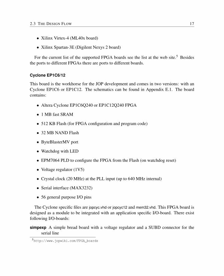
Cyclone EP1C6/12
This board is the workhorse for the JOP development and comes in two versions: with anCyclone EP1C6 or EP1C12. The schematics can be found in Appendix E.1. The boardcontains:
• Altera Cyclone EP1C6Q240 or EP1C12Q240 FPGA
• 1 MB fast SRAM
• 512 KB Flash (for FPGA configuration and program code)
• 32 MB NAND Flash
• ByteBlasterMV port
• Watchdog with LED
• EPM7064 PLD to configure the FPGA from the Flash (on watchdog reset)
• Voltage regulator (1V5)
• Crystal clock (20 MHz) at the PLL input (up to 640 MHz internal)
• Serial interface (MAX3232)
• 56 general purpose I/O pins
The Cyclone specific files are jopcyc.vhd or jopcyc12 and mem32.vhd. This FPGA board isdesigned as a module to be integrated with an application specific I/O-board. There existfollowing I/O-boards:
simpexp A simple bread board with a voltage regulator and a SUBD connector for theserial line
5http://www.jopwiki.com/FPGA_boards
18 2 THE DESIGN FLOW
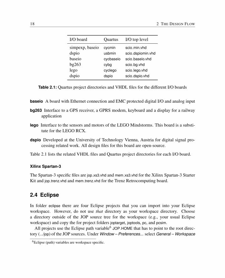
I/O board Quartus I/O top level
simpexp, baseio cycmin scio min.vhddspio usbmin scio dspiomin.vhdbaseio cycbaseio scio baseio.vhdbg263 cybg scio bg.vhdlego cyclego scio lego.vhddspio dspio scio dspio.vhd
Table 2.1: Quartus project directories and VHDL files for the different I/O boards
baseio A board with Ethernet connection and EMC protected digital I/O and analog input
bg263 Interface to a GPS receiver, a GPRS modem, keyboard and a display for a railwayapplication
lego Interface to the sensors and motors of the LEGO Mindstorms. This board is a substi-tute for the LEGO RCX.
dspio Developed at the University of Technology Vienna, Austria for digital signal pro-cessing related work. All design files for this board are open-source.
Table 2.1 lists the related VHDL files and Quartus project directories for each I/O board.
Xilinx Spartan-3
The Spartan-3 specific files are jop xs3.vhd and mem xs3.vhd for the Xilinx Spartan-3 StarterKit and jop trenz.vhd and mem trenz.vhd for the Trenz Retrocomputing board.
2.4 Eclipse
In folder eclipse there are four Eclipse projects that you can import into your Eclipseworkspace. However, do not use that directory as your workspace directory. Choosea directory outside of the JOP source tree for the workspace (e.g., your usual Eclipseworkspace) and copy the for project folders joptarget, joptools, pc, and pcsim.
All projects use the Eclipse path variable6 JOP HOME that has to point to the root direc-tory (.../jop) of the JOP sources. Under Window – Preferences... select General – Workspace
6Eclipse (path) variables are workspace specific.
2.5 SIMULATION 19
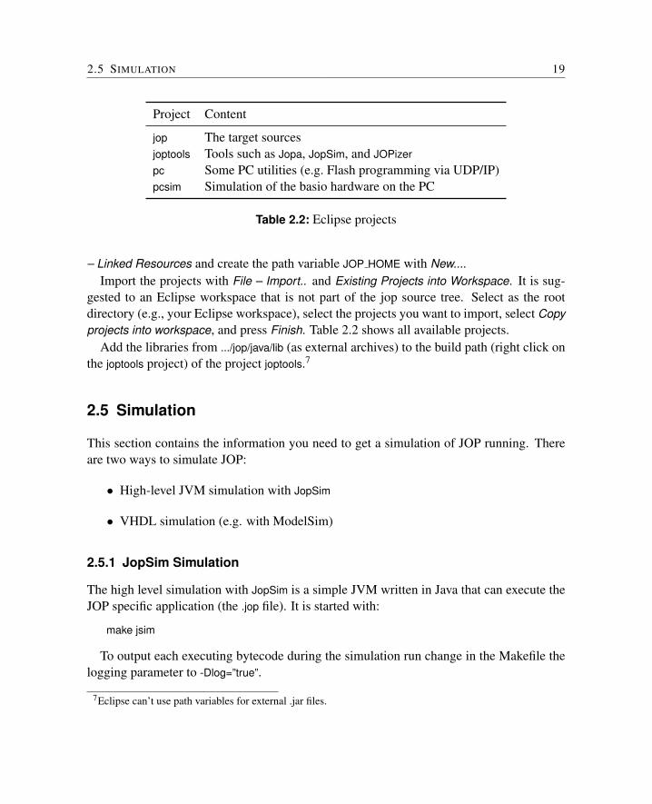
Project Content
jop The target sourcesjoptools Tools such as Jopa, JopSim, and JOPizerpc Some PC utilities (e.g. Flash programming via UDP/IP)pcsim Simulation of the basio hardware on the PC
Table 2.2: Eclipse projects
– Linked Resources and create the path variable JOP HOME with New....Import the projects with File – Import.. and Existing Projects into Workspace. It is sug-
gested to an Eclipse workspace that is not part of the jop source tree. Select as the rootdirectory (e.g., your Eclipse workspace), select the projects you want to import, select Copyprojects into workspace, and press Finish. Table 2.2 shows all available projects.
Add the libraries from .../jop/java/lib (as external archives) to the build path (right click onthe joptools project) of the project joptools.7
2.5 Simulation
This section contains the information you need to get a simulation of JOP running. Thereare two ways to simulate JOP:
• High-level JVM simulation with JopSim
• VHDL simulation (e.g. with ModelSim)
2.5.1 JopSim Simulation
The high level simulation with JopSim is a simple JVM written in Java that can execute theJOP specific application (the .jop file). It is started with:
make jsim
To output each executing bytecode during the simulation run change in the Makefile thelogging parameter to -Dlog=”true”.
7Eclipse can’t use path variables for external .jar files.
20 2 THE DESIGN FLOW
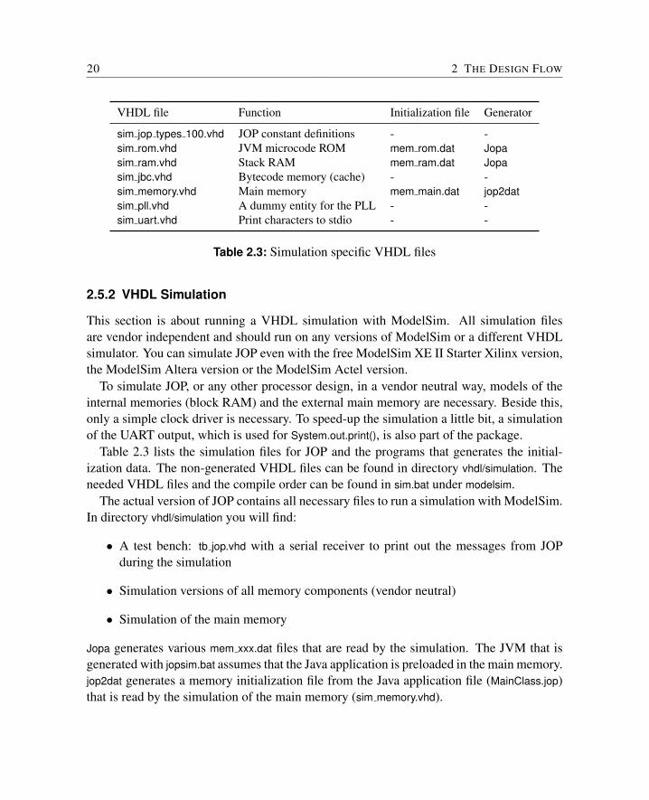
VHDL file Function Initialization file Generator
sim jop types 100.vhd JOP constant definitions - -sim rom.vhd JVM microcode ROM mem rom.dat Jopasim ram.vhd Stack RAM mem ram.dat Jopasim jbc.vhd Bytecode memory (cache) - -sim memory.vhd Main memory mem main.dat jop2datsim pll.vhd A dummy entity for the PLL - -sim uart.vhd Print characters to stdio - -
Table 2.3: Simulation specific VHDL files
2.5.2 VHDL Simulation
This section is about running a VHDL simulation with ModelSim. All simulation filesare vendor independent and should run on any versions of ModelSim or a different VHDLsimulator. You can simulate JOP even with the free ModelSim XE II Starter Xilinx version,the ModelSim Altera version or the ModelSim Actel version.
To simulate JOP, or any other processor design, in a vendor neutral way, models of theinternal memories (block RAM) and the external main memory are necessary. Beside this,only a simple clock driver is necessary. To speed-up the simulation a little bit, a simulationof the UART output, which is used for System.out.print(), is also part of the package.
Table 2.3 lists the simulation files for JOP and the programs that generates the initial-ization data. The non-generated VHDL files can be found in directory vhdl/simulation. Theneeded VHDL files and the compile order can be found in sim.bat under modelsim.
The actual version of JOP contains all necessary files to run a simulation with ModelSim.In directory vhdl/simulation you will find:
• A test bench: tb jop.vhd with a serial receiver to print out the messages from JOPduring the simulation
• Simulation versions of all memory components (vendor neutral)
• Simulation of the main memory
Jopa generates various mem xxx.dat files that are read by the simulation. The JVM that isgenerated with jopsim.bat assumes that the Java application is preloaded in the main memory.jop2dat generates a memory initialization file from the Java application file (MainClass.jop)that is read by the simulation of the main memory (sim memory.vhd).
2.6 FILES TYPES YOU MIGHT ENCOUNTER 21
In directory modelsim you will find a small batch file (sim.bat) that compiles JOP andthe test bench in the correct order and starts ModelSim. The whole simulation process(including generation of the correct microcode) is started with:
make sim
After a few seconds you should see the startup message from JOP printed in ModelSim’scommand window. The simulation can be continued with run -all and after around 6 mssimulation time the actual Java main() method is executed. During those 6 ms, which willprobably be minutes of simulation, the memory is initialized for the garbage collector.
2.6 Files Types You Might Encounter
As there are various tools involved in the complete build process, you will find files withvarious extensions. The following list explains the file types you might encounter whenchanging and building JOP.
The following files are the source files:
.vhd VHDL files describe the hardware part and are compiled with either Quartus orXilinx ISE. Simulation in ModelSim is also based on VHDL files.
.v Verilog HDL. Another hardware description language. Used more in the US.
.java Java — the language that runs native on JOP.
.c There are still some tools written in C.
.asm JOP microcode. The JVM is written in this stack oriented assembler. Files are as-sembled with Jopa. The result are VHDL files, .mif files, and .dat files for ModelSim.
.bat Usage of these DOS batch files still prohibit running the JOP build under Unix.However, these files get less used as the Makefile progresses.
.xml Project files for Ant. Ant is an attractive substitution to make. Future distributionson JOP will be ant based.
Quartus II and Xilinx ISE need configuration files that describe your project. All files areusually ASCII text files.
.qpf Quartus II Project File. Contains almost no information.
22 2 THE DESIGN FLOW
.qsf Quartus II Settings File defines the project. VHDL files that make up your projectare listed. Constraints such as pin assignments and timing constraints are set here.
.cdf Chain Description File. This file stores device name, device order, and programmingfile name information for the programmer.
.tcl Tool Command Language. Can be used in Quartus to automate parts of the designflow (e.g. pin assignment).
.npl Xilinx ISE project. VHDL files that make up your project are listed. The actualversion of Xilinx ISE converts this project file to a new format that is not in ASCIIanymore.
.ucf Xilinx Foundation User Constraint File. Constraints such as pin assignments andtiming constraints are set here.
The Java tools javac and jar produce following file types from the Java sources:
.class A class file contains the bytecodes, a symbol table and other ancillary informationand is executed by the JVM.
.jar The Java Archive file format enables you to bundle multiple files into a single archivefile. Typically a .jar file contains the class files and auxiliary resources. A .jar file isessentially a zip file that contains an optional META-INF directory.
The following files are generated by the various tools from the source files:
.jop This file makes up the linked Java application that runns on JOP. It is generated byJOPizer and can be either downloaded (serial line or USB) or stored in the Flash (orused by the simulation with JopSim or ModelSim)
.mif Memory Initialization File. Defines the initial content of on-chip block memoriesfor Altera devices.
.dat memory initialization files for the simulation with ModelSim.
.sof SRAM Output File. Configuration file for Altera devices. Used by the Quartusprogrammer or by quartus pgm. Can be converted to various (or too many) differentformat. Some are listed below.
2.7 INFORMATION ON THE WEB 23
.pof Programmer Object File. Configuration for Altera devices. Used for the Flash loaderPLDs.
.jbc JamTM STAPL Byte Code 2.0. Configuration for Altera devices. Input file for jbi32.
.ttf Tabular Text File. Configuration for Altera devices. Used by flash programmingutilities (amd and udp.Flash to store the FPGA configuration in the boards Flash.
.rbf Raw Binary File. Configuration for Altera devices. Used by the USB downloadutility (USBRunner) to configure the dspio board via the USB connection.
.bit Bitstream File. Configuration file for Xilinx devices.
2.7 Information on the Web
Further information on JOP and the build process can be found on the Internet at the fol-lowing places:
• http://www.jopdesign.com/ is the main web site for JOP
• http://www.jopwiki.com/ is a Wiki that can be freely edited by JOP users.
• http://tech.groups.yahoo.com/group/java-processor/ hosts a mailing listfor discussions on Java processors in general and mostly on JOP related topics
2.8 Porting JOP
Porting JOP to a different FPGA platform or board usually consists of adapting pin defini-tions and selection of the correct memory interface. Memory interfaces for the SimpConinterconnect can be found in directory vhdl/memory.
2.8.1 Test Utilities
To verify that the port of JOP is successful there are some small test programs in asm/src.To run the JVM on JOP the microcode jvm.asm is assembled and will be stored in an on-chip ROM. The Java application will then be loaded by the first microcode instructionsin jvm.asm into an external memory. However, to verify that JOP and the serial line areworking correctly, it is possible to run small test programs directly in microcode.
24 2 THE DESIGN FLOW
One test program (blink.asm) does not need the main memory and is a first test step beforetesting the possibly changed memory interface. testmon.asm can be used to debug the mainmemory interface. Both test programs can be built with the make targets jop blink test andjop testmon.
Blinking LED and UART output
The test is built with:
make jop blink test
After download, the watchdog LED should blink and the FPGA will print out 0 and 1 onthe serial line. Use a terminal program or the utility e.exe to check the output from the serialline.
Test Monitor
Start a terminal program (e.g. HyperTerm) to communicate with the monitor program andbuild the test monitor with:
make jop testmon
After download the program prints the content of the memory at address 0. The programunderstands following commands:
• A single CR reads the memory at the current addres and prints out the address andmemory content
• addr=val; writes val into the memory location at address addr
One tip: Take care that your terminal program does not send an LF after the CR.
2.9 Extending JOP
JOP is a soft-core processor and customizing it for an application is an interesting opportu-nity.
2.9 EXTENDING JOP 25
2.9.1 Native Methods
The native language of JOP is microcode. A native method is implemented in JOP mi-crocode. The interface to this native method is through a special bytecode. The mappingbetween native methods and the special bytecode is performed by JOPizer. When adding anew (special) bytecode to JOP, the following files have to be changed:
1. jvm.asm implementation
2. Native.java method signature
3. JopInstr.java mapping of the signature to the name
4. JopSim.java simulation of the bytecode
5. JVM.java (just rename the method name)
6. Startup.java (only when needed in a class initializer)
7. WCETInstruction.java timing information
First implement the native code in JopSim.java for easy debugging. The real microcodeis added in jvm.asm with a label for the special byctecode. The naming convention is jop-sys name. In Native.java provide a method signature for the native method and enter themapping between this signature and the name in jvm.asm and in JopInstr.java. Provide theexecution time in WCETInstruction.java for WCET analysis.
The native method is accessed by the method provided in Native.java. There is no callingoverhead involved in the mechanism. The native method gets substituted by JOPizer with aspecial bytecode.
2.9.2 A new Peripheral Device
Creation of a new peripheral devices involves some VHDL coding. However, there areseveral examples in jop/vhdl/scio available.
All peripheral components in JOP are connected with the SimpCon [127] interface. Fora device that implements the Wishbone [94] bus, a SimpCon-Wishbone bridge (sc2wb.vhd)is available (e.g., it is used to connect the AC97 interface in the dspio project).
For an easy start use an existing example and change it to your needs. Take a look intosc test slave.vhd. All peripheral components (SimpCon slaves) are connected in one moduleusually named scio xxx.vhd. Browse the examples and copy one that best fits your needs.
26 2 THE DESIGN FLOW
In this module the address of your peripheral device is defined (e.g. 0x10 for the primaryUART). This I/O address is mapped to a negative memory address for JOP. That means0xffffff80 is added as a base to the I/O address.
By convention this address mapping is defined in com.jopdesign.sys.Const. Here is theUART example:
// use negative base address for fast constant load// with bipushpublic static final int IO BASE = 0xffffff80;...public static final int IO STATUS = IO BASE+0x10;public static final int IO UART = IO BASE+0x10+1;
The I/O devices are accessed from Java by native8 functions: Native.rdMem() and Na-tive.wrMem() in pacakge com.jopdesign.sys. Again an example with the UART:
// busy wait on free tx buffer// no wait on an open serial line , just wait// on the baud ratewhile ((Native.rdMem(Const.IO STATUS)&1)==0) {
;}Native.wrMem(c, Const.IO UART);
Best practise is to create a new I/O configuration scio xxx.vhdl and a new Quartus projectfor this configuration. This avoids the mixup of the changes with a new version of JOP. Forthe new Quartus project only the three files jop.cdf, jop.qpf, and jop.qsf have to be copied in anew directory under quartus. This new directory is the project name that has to be set in theMakefile:
QPROJ=yourproject
The new VHDL module and the scio xxx.vhdl are added in jop.qsf. This file is a plainASCII file and can be edited with a standard editor or within Quartus.
2.9.3 A Customized Instruction
A customized instruction can be simply added by implementing it in microcode and map-ping it to a native function as described before. If you want to include a hardware module
8These are not real functions and are substituted by special bytecodes on application building with JOPizer.
2.9 EXTENDING JOP 27
that implements this instruction a new microinstruction has to be introduced. Besides map-ping this instruction to a native method the instruction has also be added to the microcodeassembler Jopa.
2.9.4 Dependencies and Configurations
As JOP and the JVM are a mix of VHDL and Java files, of changes some configurations orchanges in central data structures needs an update in several files.
Speed Configuration
By default, JOP is configured for 80 Mhz. To build the 100 MHz configuration, edit quar-tus/cycmin/jop.qsf and change jop config 80 to jop config 100.
Method Cache Configuration
The default configuration (for the Altera Cyclone) is a 4 KB method cache configured with16 blocks (i.e., a variable block cache). For the Xilinx targets, the cache size is 2KB becauseXilinx does not (or did not) support easily configurable block RAMs.
To change from a variable block cache to a dual-block cache, you will need to edit thetop-level VHDL. Here is an example from vhdl/top/jopcyc.vhd:
entity jop is
generic (ram cnt : integer := 2; −− clock cycles for external ram
−− rom cnt : integer := 3; −− clock cycles for external rom OK for 20 MHzrom cnt : integer := 15; −− clock cycles for external rom for 100 MHzjpc width : integer := 12; −− address bits of java bytecode pc = cache sizeblock bits : integer := 4 −− 2∗block bits is number of cache blocks
);
The power of 2 of the jpc width is the cache size, and the power of 2 of the block bits is thenumber of blocks. To simulate a dual block cache, block bits has to be set to 1. (To use asingle block cache, cache.vhd has to be modified to force a miss at the cache lookup.)
Stack Size
The on-chip stack size can be configured by changing following constants:
28 2 THE DESIGN FLOW
• ram width in jop config xx.vhd
• STACK SIZE in com.jopdesign.sys.Const
• RAM LEN in com.jopdesign.sys.Jopa
Changing the Class Format
The constants for the offsets of fields in the class format are found in:
• JOPizer: CLS HEAD, dump()
• GC.java uses CLASS HEADR
• JMV.java uses CLASS HEADR + offset (checkcast, instanceof)
2.10 Directory Structure
The top-level directories of the distribution are:
asm Microcode source files. The microcode part of the JVM and test files.
boards Pictures and text for the Eclipse plugin
c src Some utilities in C (e.g. down.exe and e.exe).
doc LATEXsources for this handbook and short notes.
eclipse Eclipse project files
ext External VHDL and Verilog sources
java All Java files
lib External .jar filespc Tools on the PCpcsim High-level simulation on the PCtarget The Java sources for JOPtools All Java tools
jbc FPGA configuration files for jbi32.exe (generated)
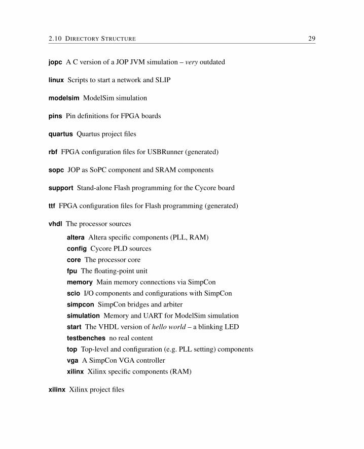
2.10 DIRECTORY STRUCTURE 29
jopc A C version of a JOP JVM simulation – very outdated
linux Scripts to start a network and SLIP
modelsim ModelSim simulation
pins Pin definitions for FPGA boards
quartus Quartus project files
rbf FPGA configuration files for USBRunner (generated)
sopc JOP as SoPC component and SRAM components
support Stand-alone Flash programming for the Cycore board
ttf FPGA configuration files for Flash programming (generated)
vhdl The processor sources
altera Altera specific components (PLL, RAM)
config Cycore PLD sources
core The processor core
fpu The floating-point unit
memory Main memory connections via SimpCon
scio I/O components and configurations with SimpCon
simpcon SimpCon bridges and arbiter
simulation Memory and UART for ModelSim simulation
start The VHDL version of hello world – a blinking LED
testbenches no real content
top Top-level and configuration (e.g. PLL setting) components
vga A SimpCon VGA controller
xilinx Xilinx specific components (RAM)
xilinx Xilinx project files
30 2 THE DESIGN FLOW
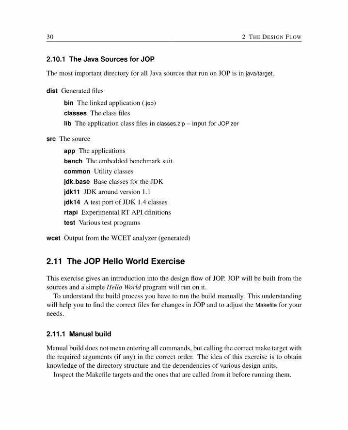
2.10.1 The Java Sources for JOP
The most important directory for all Java sources that run on JOP is in java/target.
dist Generated files
bin The linked application (.jop)classes The class fileslib The application class files in classes.zip – input for JOPizer
src The source
app The applicationsbench The embedded benchmark suitcommon Utility classesjdk base Base classes for the JDKjdk11 JDK around version 1.1jdk14 A test port of JDK 1.4 classesrtapi Experimental RT API dfinitionstest Various test programs
wcet Output from the WCET analyzer (generated)
2.11 The JOP Hello World Exercise
This exercise gives an introduction into the design flow of JOP. JOP will be built from thesources and a simple Hello World program will run on it.
To understand the build process you have to run the build manually. This understandingwill help you to find the correct files for changes in JOP and to adjust the Makefile for yourneeds.
2.11.1 Manual build
Manual build does not mean entering all commands, but calling the correct make target withthe required arguments (if any) in the correct order. The idea of this exercise is to obtainknowledge of the directory structure and the dependencies of various design units.
Inspect the Makefile targets and the ones that are called from it before running them.
2.11 THE JOP HELLO WORLD EXERCISE 31
1. Create your working directory
2. Download the sources from the opencores CVS server
3. Connect the FPGA board to the PC (and the power supply)
4. Perform the build as described in Section 2.1.2.
As a result you should see a message at your command prompt.
2.11.2 Using make
In the root directory (jop) there is a Makefile. Open it with an editor and try to find thecorresponding lines of code for the steps you did in the first exercise. Reset the FPGA bycycling the power and run the build with a simple
make
The whole process should run without errors and the result should be identical to theprevious exercise.
2.11.3 Change the Java Program
The whole build process is not necessary when changing the Java application. Once theprocessor is built, a Java application can be built and downloaded with the following maketarget:
make japp
Change HelloWorld.java and run it on JOP. Now change the class name that contains the main()method from HelloWorld to Hello and rerun the Java application build. Now an embeddedversion of “Hello World” should run on JOP. Besides the usual greeting on the standardoutput, the LED on the FPGA board should blink at a frequency of 1 Hz. The first periodictask, an essential abstraction for real-time systems, is running on JOP!
2.11.4 Change the Microcode
The JVM is written in microcode and several .vhdl files are generated during assembly. Fora test change only the version string9 in jvm.asm to the actual date and run a full make.
9The actual version date will probably be different from the actual sources.
32 2 THE DESIGN FLOW
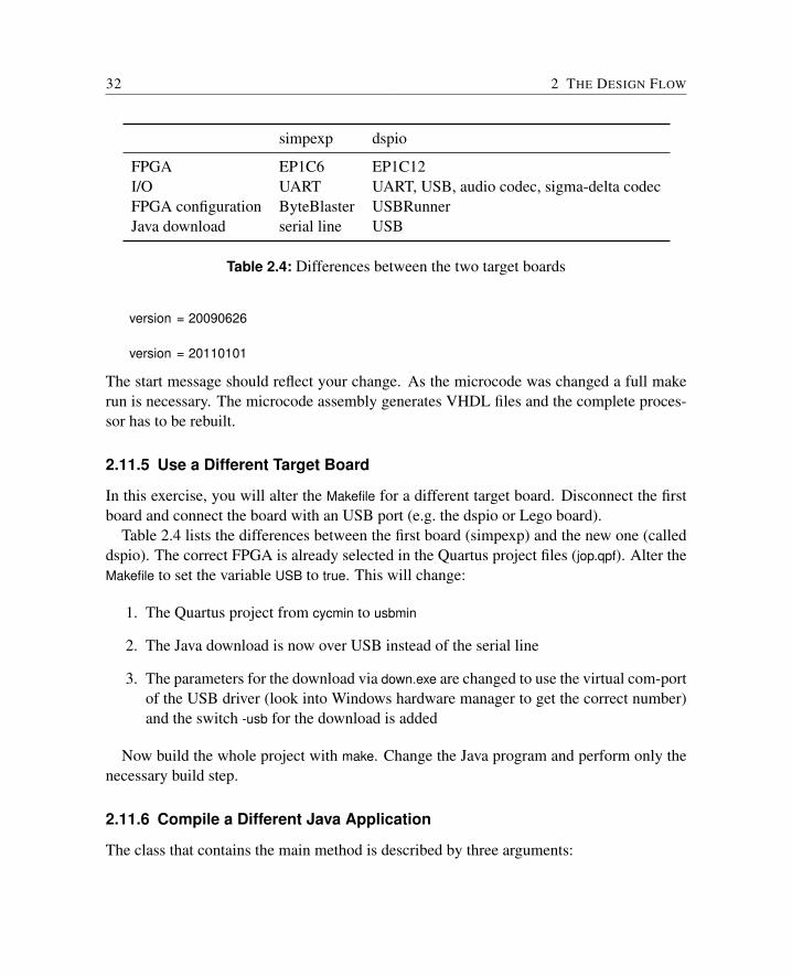
simpexp dspio
FPGA EP1C6 EP1C12I/O UART UART, USB, audio codec, sigma-delta codecFPGA configuration ByteBlaster USBRunnerJava download serial line USB
Table 2.4: Differences between the two target boards
version = 20090626
version = 20110101
The start message should reflect your change. As the microcode was changed a full makerun is necessary. The microcode assembly generates VHDL files and the complete proces-sor has to be rebuilt.
2.11.5 Use a Different Target Board
In this exercise, you will alter the Makefile for a different target board. Disconnect the firstboard and connect the board with an USB port (e.g. the dspio or Lego board).
Table 2.4 lists the differences between the first board (simpexp) and the new one (calleddspio). The correct FPGA is already selected in the Quartus project files (jop.qpf). Alter theMakefile to set the variable USB to true. This will change:
1. The Quartus project from cycmin to usbmin
2. The Java download is now over USB instead of the serial line
3. The parameters for the download via down.exe are changed to use the virtual com-portof the USB driver (look into Windows hardware manager to get the correct number)and the switch -usb for the download is added
Now build the whole project with make. Change the Java program and perform only thenecessary build step.
2.11.6 Compile a Different Java Application
The class that contains the main method is described by three arguments:
2.11 THE JOP HELLO WORLD EXERCISE 33
1. The first directory relative to java/target/src (e.g. app or test)
2. The package name (e.g. dsp)
3. The main class (e.g. HalloWorld)
These three values are used by the Makeile and are set in the variables P1, P2, and P3 inthe Makefile.
Change the Makefile to compile the embedded Java benchmark jbe.DoAll. The parame-ters for the Java application can also be given to the make with following command linearguments:
make −e P1=bench P2=jbe P3=DoAll
The three variables P1, P2, and P3 are a shortcut to set the main class of the application.You can also directly set the variables TARGET APP PATH and MAIN CLASS.
2.11.7 Simulation
This exercise will give you a full view of the possibilities to debug JOP system code or theprocessor itself. There are two ways to simulate JOP: A simple debugging JVM written inJava (JopSim as part of the tool package) that can execute jopized applications and a VHDLlevel simulation with ModelSim. The make targets are jsim and sim.
2.11.8 WCET Analysis
An important step in real-time system development is the analysis of the WCET of theindividual tasks. Compile and run the WCET example Loop.java in package wcet. You cananalyze the WCET of the method measure() with following make command:
make java app wcet −e P1=test P2=wcet P3=Loop
Change the code in Loop.java to enable measurement of the execution time and compare itwith the output of the static analysis. In this simple example the WCET can be measured.However, be aware that most non-trivial code needs static analysis for safe estimates ofWCET values.

3 Java and the Java Virtual Machine
Java technology consists of the Java language definition, a definition of the standard li-brary, and the definition of an intermediate instruction set with an accompanying executionenvironment. This combination helps to make write once, run anywhere possible.
The following chapter gives a short overview of the Java programming language. A moredetailed description of the Java Virtual Machine (JVM) and the explanation of the JVMinstruction set, the so-called bytecodes, follows. The exploration of dynamic instructioncounts of typical Java programs can be found in Section ??.
3.1 Java
Java is a relatively new and popular programming language. The main features that havehelped Java achieve success are listed below:
Simple and object oriented: Java is a simple programming language that appears verysimilar to C. This ‘look and feel’ of C means that programmers who know C, canswitch to Java without difficulty. Java provides a simplified object model with singleinheritance1.
Portability: To accommodate the diversity of operating environments, the Java compilergenerates bytecodes – an architecture neutral intermediate format. To guarantee plat-form independence, Java specifies the sizes of its basic data types and the behavior ofits arithmetic operators. A Java interpreter, the Java virtual machine, is available onvarious platforms to help make ‘write once, run anywhere’ possible.
Availability: Java is not only available for different operating systems, it is available at nocost. The runtime system and the compiler can be downloaded from Sun’s websitefor Windows, Linux, and Solaris. Sophisticated development environments, such asNetbeans or Eclipse, are available under the GNU Public License.
1Java has single inheritance of implementation – only one class can be extended. However, a class canimplement several interfaces, which means that Java has multiple interface inheritance.
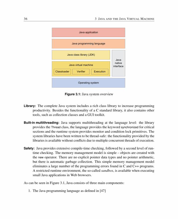
36 3 JAVA AND THE JAVA VIRTUAL MACHINE
Operating system
Java virtual machine
Javanative
interface
Java class library (JDK)
Java application
Java programming language
Classloader Verifier Execution
Figure 3.1: Java system overview
Library: The complete Java system includes a rich class library to increase programmingproductivity. Besides the functionality of a C standard library, it also contains othertools, such as collection classes and a GUI toolkit.
Built-in multithreading: Java supports multithreading at the language level: the libraryprovides the Thread class, the language provides the keyword synchronized for criticalsections and the runtime system provides monitor and condition lock primitives. Thesystem libraries have been written to be thread-safe: the functionality provided by thelibraries is available without conflicts due to multiple concurrent threads of execution.
Safety: Java provides extensive compile-time checking, followed by a second level of run-time checking. The memory management model is simple – objects are created withthe new operator. There are no explicit pointer data types and no pointer arithmetic,but there is automatic garbage collection. This simple memory management modeleliminates a large number of the programming errors found in C and C++ programs.A restricted runtime environment, the so-called sandbox, is available when executingsmall Java applications in Web browsers.
As can be seen in Figure 3.1, Java consists of three main components:
1. The Java programming language as defined in [47]
3.1 JAVA 37
2. The class library, defined as part of the Java specification. All implementations ofJava have to contain the library as defined by Sun
3. The Java virtual machine (defined in [82]) that loads, verifies and executes the binaryrepresentation (the class file) of a Java program
The Java native interface supports functions written in C or C++. This combination issometimes called Java technology to emphasize the fact that Java is more than just anotherobject-oriented language.
However, a number of issues have slowed down the broad acceptance of Java. The orig-inal presentation of Java as an Internet language led to the misconception that Java wasnot a general-purpose programming language. Another obstacle was the first implementa-tion of the JVM as an interpreter. Execution of Java programs was very slow compared tocompiled C/C++ programs. Although advances in its runtime technology, in particular thejust-in-time compiler, have closed the performance gap, it is still a commonly held viewthat Java is slow.
3.1.1 History
The Java programming language originated as part of the Green project specifically for anembedded device, a handheld wireless PDA. In the early ’90s, Java, which was originallyknown as Oak [143, 144], was created as the programming tool for this device. The device(known as *7) was a small SPARC-based hardware device with a tiny embedded OS. How-ever, the *7 was never released as a product and Java was officially released in 1995 as thenew language for the Internet. Over the years, Java technology has become a programmingtool for desktop applications, web servers and server applications. These application do-mains resulted in the split of the Java platform into the Java standard edition (J2SE) and theenterprise edition (J2EE) in 1999. With every new release, the library (defined as part ofthe language) continued to grow. Java for embedded systems was clearly not an area Sunwas interested in pursuing. However, with the arrival of mobile phones, Sun again becameinterested in this embedded market. Sun defined different subsets of Java, which have nowbeen combined into the Java Micro Edition (J2ME).
In 1999, a document defining the requirements for real-time Java was published by theNIST [88]. Based on these requirements, two groups defined specifications for real-timeJava: the Real-Time Core Extension [141] published under the J Consortium and the Real-Time Specification for Java (RTSJ) [25]. A comparison of these two specifications and acomparison with Ada 95’s Real-Time Annex can be found in [30]. The RTSJ was the firstJava Specification Request (JSR 1) under the Java Community Process (JCP) and started
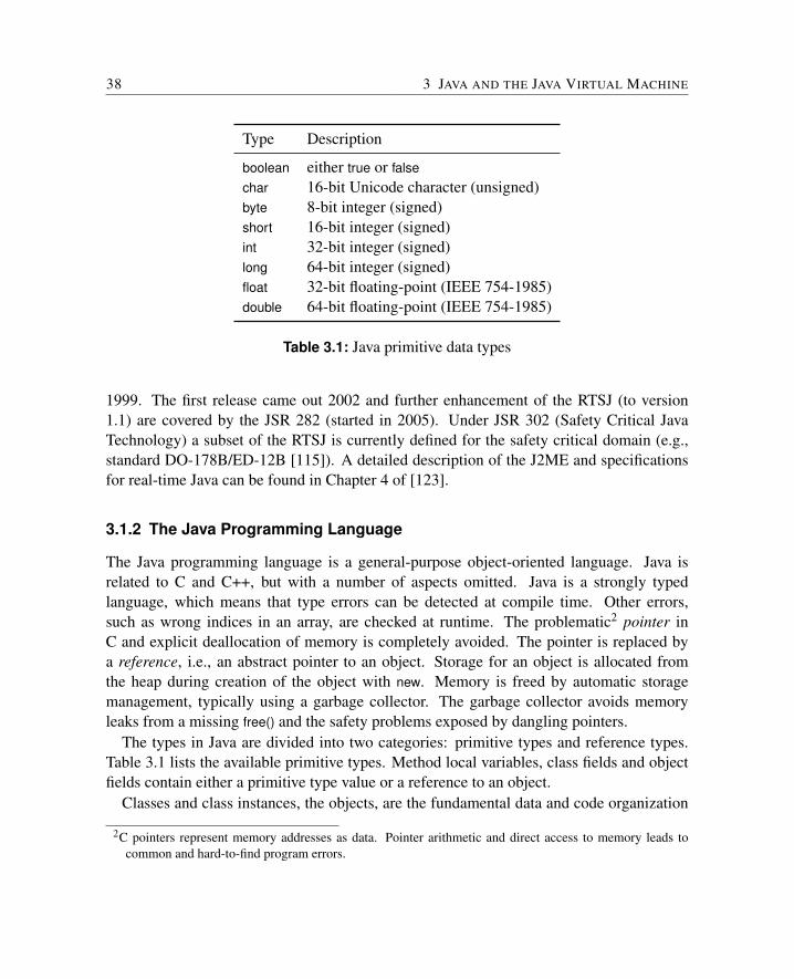
38 3 JAVA AND THE JAVA VIRTUAL MACHINE
Type Description
boolean either true or falsechar 16-bit Unicode character (unsigned)byte 8-bit integer (signed)short 16-bit integer (signed)int 32-bit integer (signed)long 64-bit integer (signed)float 32-bit floating-point (IEEE 754-1985)double 64-bit floating-point (IEEE 754-1985)
Table 3.1: Java primitive data types
1999. The first release came out 2002 and further enhancement of the RTSJ (to version1.1) are covered by the JSR 282 (started in 2005). Under JSR 302 (Safety Critical JavaTechnology) a subset of the RTSJ is currently defined for the safety critical domain (e.g.,standard DO-178B/ED-12B [115]). A detailed description of the J2ME and specificationsfor real-time Java can be found in Chapter 4 of [123].
3.1.2 The Java Programming Language
The Java programming language is a general-purpose object-oriented language. Java isrelated to C and C++, but with a number of aspects omitted. Java is a strongly typedlanguage, which means that type errors can be detected at compile time. Other errors,such as wrong indices in an array, are checked at runtime. The problematic2 pointer inC and explicit deallocation of memory is completely avoided. The pointer is replaced bya reference, i.e., an abstract pointer to an object. Storage for an object is allocated fromthe heap during creation of the object with new. Memory is freed by automatic storagemanagement, typically using a garbage collector. The garbage collector avoids memoryleaks from a missing free() and the safety problems exposed by dangling pointers.
The types in Java are divided into two categories: primitive types and reference types.Table 3.1 lists the available primitive types. Method local variables, class fields and objectfields contain either a primitive type value or a reference to an object.
Classes and class instances, the objects, are the fundamental data and code organization
2C pointers represent memory addresses as data. Pointer arithmetic and direct access to memory leads tocommon and hard-to-find program errors.
3.2 THE JAVA VIRTUAL MACHINE 39
structures in Java. There are no global variables or functions as there are in C/C++. Eachmethod belongs to a class. This ‘everything belongs to a class or an object’ combined withthe class naming convention, as suggested by Sun, avoids name conflicts in even the largestapplications.
New classes can extend exactly one superclass. Classes that do not explicitly extend asuperclass become direct subclasses of Object, the root of the whole class tree. This singleinheritance model is extended by interfaces. Interfaces are abstract classes that only definemethod signatures and provide no implementation. A concrete class can implement severalinterfaces. This model provides a simplified form of multiple inheritance.
Java supports multitasking through threads. Each thread is a separate flow of control,executing concurrently with all other threads. A thread contains the method stack as threadlocal data – all objects are shared between threads. Access conflicts to shared data areavoided by the proper use of synchronized methods or code blocks.
Java programs are compiled to a machine-independent bytecode representation as definedin [82]. Although this intermediate representation is defined for Java, other programminglanguages (e.g., ADA [33]) can also be compiled into Java bytecodes.
3.2 The Java Virtual Machine
The Java virtual machine (JVM) is a definition of an abstract computing machine that exe-cutes bytecode programs. The JVM specification [82] defines three elements:
• An instruction set and the meaning of those instructions – the bytecodes
• A binary format – the class file format. A class file contains the bytecodes, a symboltable and other ancillary information
• An algorithm to verify that a class file contains valid programs
In the solution presented in this book, the class files are verified, linked and transformed intoan internal representation before being executed on JOP. This transformation is performedwith JOPizer and is not executed on JOP. We will therefore omit the description of the classfile and the verification process.
The instruction set of the JVM is stack-based. All operations take their arguments fromthe stack and put the result onto the stack. Values are transferred between the stack andvarious memory areas. We will discuss these memory areas first, followed by an explanationof the instruction set.
40 3 JAVA AND THE JAVA VIRTUAL MACHINE
3.2.1 Memory Areas
The JVM contains various runtime data areas. Some of these areas are shared betweenthreads, whereas other data areas exist separately for each thread.
Method area: The method area is shared among all threads. It contains static class in-formation such as field and method data, the code for the methods and the constantpool. The constant pool is a per-class table, containing various kinds of constantssuch as numeric values or method and field references. The constant pool is similarto a symbol table.
Part of this area, the code for the methods, is very frequently accessed (during in-struction fetch) and therefore is a good candidate for caching.
Heap: The heap is the data area where all objects and arrays are allocated. The heap isshared among all threads. A garbage collector reclaims storage for objects.
JVM stack: Each thread has a private stack area that is created at the same time as thethread. The JVM stack is a logical stack that contains following elements:
1. A frame that contains return information for a method2. A local variable area to hold local values inside a method3. The operand stack, where all operations are performed
Although it is not strictly necessary to allocate all three elements to the same type ofmemory we will see in Section 4.4 that the argument-passing mechanism regulatesthe layout of the JVM stack.
Local variables and the operand stack are accessed as frequently as registers in astandard processor. A Java processor should provide some caching mechanism ofthis data area.
The memory areas are similar to the various segments in conventional processes (e.g. themethod code is analogous to the ‘text’ segment). However, the operand stack replaces theregisters in a conventional processor.
3.2.2 JVM Instruction Set
The instruction set of the JVM contains 201 different instructions [82]. This bytecodes canbe grouped into the following categories:
3.2 THE JAVA VIRTUAL MACHINE 41
Load and store: Load instructions push values from the local variables onto the operandstack. Store instructions transfer values from the stack back to local variables. 70different instructions belong to this category. Short versions (single byte) exist toaccess the first four local variables. There are unique instructions for each basic type(int, long, float, double and reference). This differentiation is necessary for the bytecodeverifier, but is not needed during execution. For example iload, fload and aload alltransfer one 32-bit word from a local variable to the operand stack.
Arithmetic: The arithmetic instructions operate on the values found on the stack and pushthe result back onto the operand stack. There are arithmetic instructions for int, floatand double. There is no direct support for byte, short or char types. These values arehandled by int operations and have to be converted back before being stored in a localvariable or an object field.
Type conversion: The type conversion instructions perform numerical conversions be-tween all Java types: as implicit widening conversions (e.g., int to long, float or double)or explicit (by casting to a type) narrowing conversions.
Object creation and manipulation: Class instances and arrays (that are also objects) arecreated and manipulated with different instructions. Objects and class fields are ac-cessed with type-less instructions.
Operand stack manipulation: All direct stack manipulation instructions are type-less andoperate on 32-bit or 64-bit entities on the stack. Examples of these instructions aredup, to duplicate the top operand stack value, and pop, to remove the top operandstack value.
Control transfer: Conditional and unconditional branches cause the JVM to continue ex-ecution with an instruction other than the one immediately following. Branch tar-get addresses are specified relative to the current address with a signed 16-bit off-set. The JVM provides a complete set of branch conditions for int values and refer-ences. Floating-point values and type long are supported through compare instruc-tions. These compare instructions result in an int value on the operand stack.
Method invocation and return: The different types of methods are supported by four in-structions: invoke a class method, invoke an instance method, invoke a method thatimplements an interface and an invokespecial for an instance method that requires spe-cial handling, such as private methods or a superclass method.
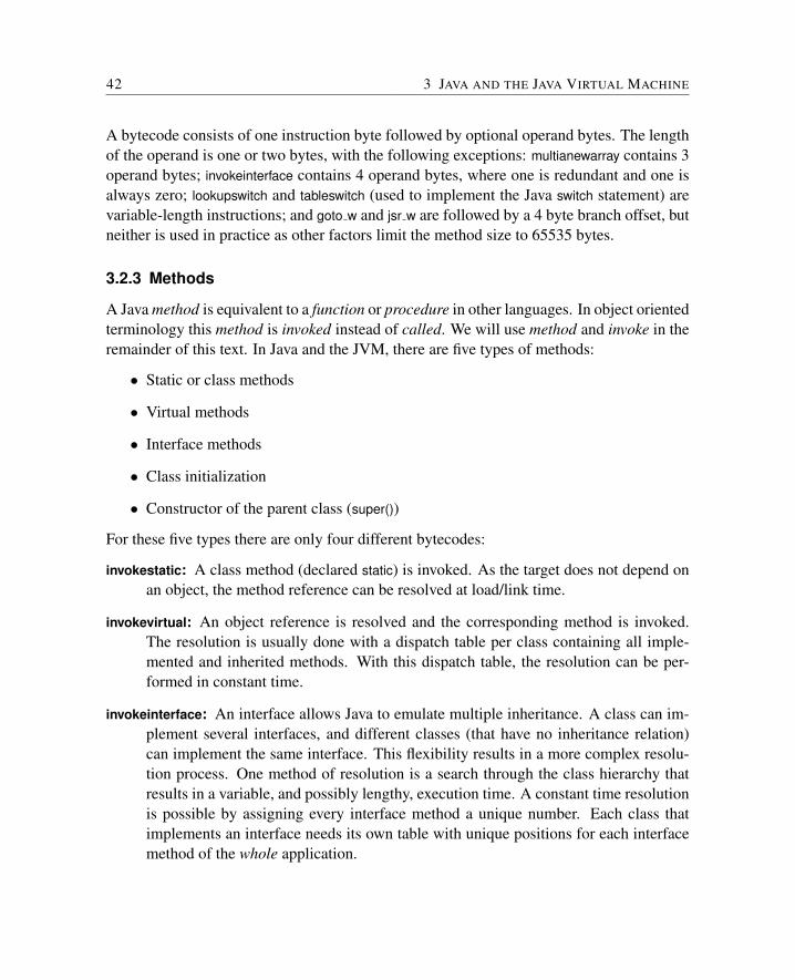
42 3 JAVA AND THE JAVA VIRTUAL MACHINE
A bytecode consists of one instruction byte followed by optional operand bytes. The lengthof the operand is one or two bytes, with the following exceptions: multianewarray contains 3operand bytes; invokeinterface contains 4 operand bytes, where one is redundant and one isalways zero; lookupswitch and tableswitch (used to implement the Java switch statement) arevariable-length instructions; and goto w and jsr w are followed by a 4 byte branch offset, butneither is used in practice as other factors limit the method size to 65535 bytes.
3.2.3 Methods
A Java method is equivalent to a function or procedure in other languages. In object orientedterminology this method is invoked instead of called. We will use method and invoke in theremainder of this text. In Java and the JVM, there are five types of methods:
• Static or class methods
• Virtual methods
• Interface methods
• Class initialization
• Constructor of the parent class (super())
For these five types there are only four different bytecodes:
invokestatic: A class method (declared static) is invoked. As the target does not depend onan object, the method reference can be resolved at load/link time.
invokevirtual: An object reference is resolved and the corresponding method is invoked.The resolution is usually done with a dispatch table per class containing all imple-mented and inherited methods. With this dispatch table, the resolution can be per-formed in constant time.
invokeinterface: An interface allows Java to emulate multiple inheritance. A class can im-plement several interfaces, and different classes (that have no inheritance relation)can implement the same interface. This flexibility results in a more complex resolu-tion process. One method of resolution is a search through the class hierarchy thatresults in a variable, and possibly lengthy, execution time. A constant time resolutionis possible by assigning every interface method a unique number. Each class thatimplements an interface needs its own table with unique positions for each interfacemethod of the whole application.
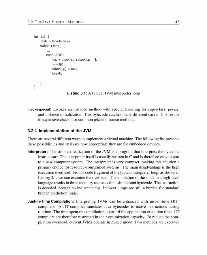
3.2 THE JAVA VIRTUAL MACHINE 43
for (;;) {instr = bcode[pc++];switch ( instr ) {
...case IADD:
tos = stack[sp]+stack[sp−1];−−sp;stack[sp] = tos;break;
...}
}Listing 3.1: A typical JVM interpreter loop
invokespecial: Invokes an instance method with special handling for superclass, private,and instance initialization. This bytecode catches many different cases. This resultsin expensive checks for common private instance methods.
3.2.4 Implementation of the JVM
There are several different ways to implement a virtual machine. The following list presentsthese possibilities and analyses how appropriate they are for embedded devices.
Interpreter: The simplest realization of the JVM is a program that interprets the bytecodeinstructions. The interpreter itself is usually written in C and is therefore easy to portto a new computer system. The interpreter is very compact, making this solution aprimary choice for resource-constrained systems. The main disadvantage is the highexecution overhead. From a code fragment of the typical interpreter loop, as shown inListing 3.1, we can examine the overhead: The emulation of the stack in a high-levellanguage results in three memory accesses for a simple iadd bytecode. The instructionis decoded through an indirect jump. Indirect jumps are still a burden for standardbranch prediction logic.
Just-In-Time Compilation: Interpreting JVMs can be enhanced with just-in-time (JIT)compilers. A JIT compiler translates Java bytecodes to native instructions duringruntime. The time spent on compilation is part of the application execution time. JITcompilers are therefore restricted in their optimization capacity. To reduce the com-pilation overhead, current JVMs operate in mixed mode: Java methods are executed
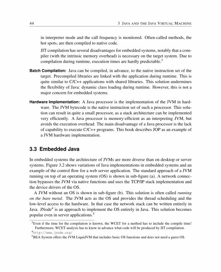
44 3 JAVA AND THE JAVA VIRTUAL MACHINE
in interpreter mode and the call frequency is monitored. Often-called methods, thehot spots, are then compiled to native code.
JIT compilation has several disadvantages for embedded systems, notably that a com-piler (with the intrinsic memory overhead) is necessary on the target system. Due tocompilation during runtime, execution times are hardly predictable.3
Batch Compilation: Java can be compiled, in advance, to the native instruction set of thetarget. Precompiled libraries are linked with the application during runtime. This isquite similar to C/C++ applications with shared libraries. This solution underminesthe flexibility of Java: dynamic class loading during runtime. However, this is not amajor concern for embedded systems.
Hardware Implementation: A Java processor is the implementation of the JVM in hard-ware. The JVM bytecode is the native instruction set of such a processor. This solu-tion can result in quite a small processor, as a stack architecture can be implementedvery efficiently. A Java processor is memory-efficient as an interpreting JVM, butavoids the execution overhead. The main disadvantage of a Java processor is the lackof capability to execute C/C++ programs. This book describes JOP as an example ofa JVM hardware implementation.
3.3 Embedded Java
In embedded systems the architecture of JVMs are more diverse than on desktop or serversystems. Figure 3.2 shows variations of Java implementations in embedded systems and anexample of the control flow for a web server application. The standard approach of a JVMrunning on top of an operating system (OS) is shown in sub-figure (a). A network connec-tion bypasses the JVM via native functions and uses the TCP/IP stack implementation andthe device drivers of the OS.
A JVM without an OS is shown in sub-figure (b). This solution is often called runningon the bare metal. The JVM acts as the OS and provides the thread scheduling and thelow-level access to the hardware. In that case the network stack can be written entirely inJava. JNode4 is an approach to implement the OS entirely in Java. This solution becomespopular even in server applications.5
3Even if the time for the compilation is known, the WCET for a method has to include the compile time!Furthermore, WCET analysis has to know in advance what code will be produced by JIT compilation.
4http://www.jnode.org/5BEA System offers the JVM LiquidVM that includes basic OS functions and does not need a guest OS.
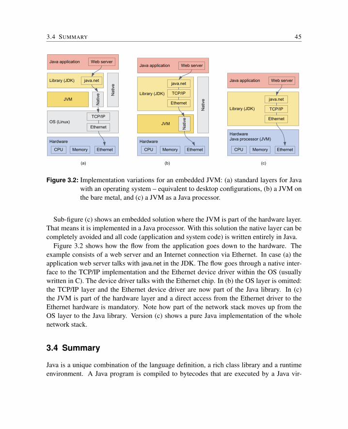
3.4 SUMMARY 45
HardwareJava processor (JVM)
Library (JDK)
CPU Memory Ethernet
java.net
TCP/IP
Ethernet
Java application Web server
Hardware
OS (Linux)
JVM
Nat
ive
Library (JDK)
CPU Memory Ethernet
java.net
TCP/IP
Ethernet
Java application
Nat
ive
Web server
Hardware
JVM
Nat
ive
Library (JDK)
CPU Memory Ethernet
java.net
TCP/IP
Ethernet
Java application
Nat
ive
Web server
(a) (b) (c)
Figure 3.2: Implementation variations for an embedded JVM: (a) standard layers for Javawith an operating system – equivalent to desktop configurations, (b) a JVM onthe bare metal, and (c) a JVM as a Java processor.
Sub-figure (c) shows an embedded solution where the JVM is part of the hardware layer.That means it is implemented in a Java processor. With this solution the native layer can becompletely avoided and all code (application and system code) is written entirely in Java.
Figure 3.2 shows how the flow from the application goes down to the hardware. Theexample consists of a web server and an Internet connection via Ethernet. In case (a) theapplication web server talks with java.net in the JDK. The flow goes through a native inter-face to the TCP/IP implementation and the Ethernet device driver within the OS (usuallywritten in C). The device driver talks with the Ethernet chip. In (b) the OS layer is omitted:the TCP/IP layer and the Ethernet device driver are now part of the Java library. In (c)the JVM is part of the hardware layer and a direct access from the Ethernet driver to theEthernet hardware is mandatory. Note how part of the network stack moves up from theOS layer to the Java library. Version (c) shows a pure Java implementation of the wholenetwork stack.
3.4 Summary
Java is a unique combination of the language definition, a rich class library and a runtimeenvironment. A Java program is compiled to bytecodes that are executed by a Java vir-
46 3 JAVA AND THE JAVA VIRTUAL MACHINE
tual machine. Strong typing, runtime checks and avoidance of pointers make Java a safelanguage. The intermediate bytecode representation simplifies porting of Java to differentcomputer systems. An interpreting JVM is easy to implement and needs few system re-sources. However, the execution speed suffers from interpreting. JVMs with a just-in-timecompiler are state-of-the-art for desktop and server systems. These compilers require largeamounts of memory and have to be ported for each processor architecture, which meansthey are not the best choice for embedded systems. A Java processor is the implementationof the JVM as a concrete machine. A Java processor avoids the slow execution model of aninterpreting JVM and the memory requirements of a compiler, thus making it an interestingexecution system for Java in embedded systems.
4 Hardware Architecture
This chapter presents the architecture of JOP and the motivation behind the various dif-ferent design decisions we faced. The first sections give an overview of JOP, describe themicrocode and the pipeline.
Pipelined instruction processing calls for high memory bandwidth. Caches are needed inorder to avoid bottlenecks resulting from the main memory bandwidth. As seen in Chap-ter 3, there are two memory areas that are frequently accessed by the JVM: the stack andthe method area. In this chapter, time-predictable cache solutions for both areas that areimplemented in JOP are presented.
4.1 Overview of JOP
This section gives an overview of JOP architecture. Figure 4.1 shows JOP’s major functionunits. A typical configuration of JOP contains the processor core, a memory interface anda number of I/O devices. The module extension provides the link between the processorcore, and the memory and I/O modules.
The processor core contains the three microcode pipeline stages microcode fetch, decodeand execute and an additional translation stage bytecode fetch. The ports to the other mod-ules are the two top elements of the stack (TOS and NOS), input to the top-of-stack (Data),bytecode cache address and data, and a number of control signals. There is no direct con-nection between the processor core and the external world.
The memory controller implements the simple memory load and store operations andthe field and array access bytecodes. It also contains the method cache. The memory in-terface provides a connection between the main memory and the memory controller. Theextension module controls data read and write. The busy signal is used by the microcodeinstruction wait1 to synchronize the processor core with the memory unit. The core readsbytecode instructions through dedicated buses (BC address and BC data) from the memory
1The busy signal can also be used to stall the whole processor pipeline. This was the change made to JOP byFlavius Gruian [48]. However, in this synchronization mode, the concurrency between the memory accessmodule and the main pipeline is lost.
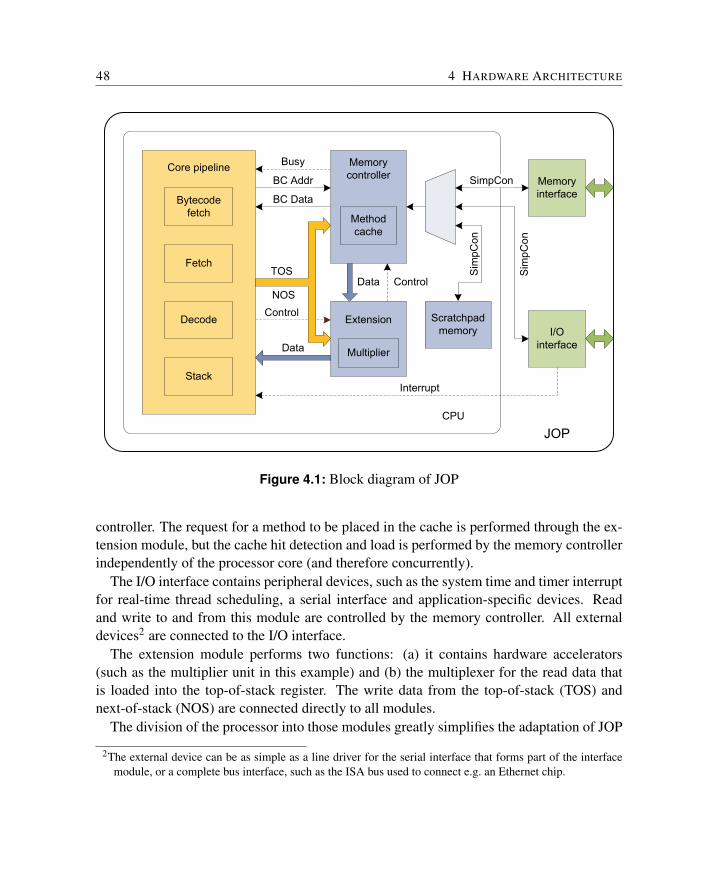
48 4 HARDWARE ARCHITECTURE
Control
JOP
Busy
BC Addr
BC Data
CPU
Scratchpadmemory I/O
interface
Memoryinterface
Data
Extension
Multiplier
Memorycontroller
Methodcache
SimpCon
Sim
pCon
Sim
pCon
Data
Interrupt
Control
Core pipeline
Bytecodefetch
Fetch
Decode
Stack
TOS
NOS
Figure 4.1: Block diagram of JOP
controller. The request for a method to be placed in the cache is performed through the ex-tension module, but the cache hit detection and load is performed by the memory controllerindependently of the processor core (and therefore concurrently).
The I/O interface contains peripheral devices, such as the system time and timer interruptfor real-time thread scheduling, a serial interface and application-specific devices. Readand write to and from this module are controlled by the memory controller. All externaldevices2 are connected to the I/O interface.
The extension module performs two functions: (a) it contains hardware accelerators(such as the multiplier unit in this example) and (b) the multiplexer for the read data thatis loaded into the top-of-stack register. The write data from the top-of-stack (TOS) andnext-of-stack (NOS) are connected directly to all modules.
The division of the processor into those modules greatly simplifies the adaptation of JOP
2The external device can be as simple as a line driver for the serial interface that forms part of the interfacemodule, or a complete bus interface, such as the ISA bus used to connect e.g. an Ethernet chip.
4.2 MICROCODE 49
for different application domains or hardware platforms. Porting JOP to a new FPGA boardusually results in changes in the memory interface alone. Using the same board for differentapplications only involves making changes to the I/O interface. JOP has been ported toseveral different FPGAs and prototyping boards and has been used in different real-worldapplications (see Chapter 11), but it never proved necessary to change the processor core.
4.2 Microcode
The following discussion concerns two different instruction sets: bytecode and microcode.Bytecodes are the instructions that make up a compiled Java program. These instructionsare executed by a Java virtual machine. The JVM does not assume any particular im-plementation technology. Microcode is the native instruction set for JOP. Bytecodes aretranslated, during their execution, into JOP microcode. Both instruction sets are designedfor an extended3 stack machine.
4.2.1 Translation of Bytecodes to Microcode
To date, no hardware implementation of the JVM exists that is capable of executing allbytecodes in hardware alone. This is due to the following: some bytecodes, such as new,which creates and initializes a new object, are too complex to implement in hardware. Thesebytecodes have to be emulated by software.
To build a self contained JVM without an underlying operating system, direct access tothe memory and I/O devices is necessary. There are no bytecodes defined for low-levelaccess. These low-level services are usually implemented in native functions, which meansthat another language (C) is native to the processor. However, for a Java processor, bytecodeis the native language.
One way to solve this problem is to implement simple bytecodes in hardware and toemulate the more complex and native functions in software with a different instruction set(sometimes called microcode). However, a processor with two different instruction setsresults in a complex design.
Another common solution, used in Sun’s picoJava [145], is to execute a subset of thebytecode native and to use a software trap to execute the remainder. This solution entailsan overhead (a minimum of 16 cycles in picoJava, see 12.2.1) for the software trap.
3An extended stack machine is one in which there are instructions available to access elements deeper downin the stack.
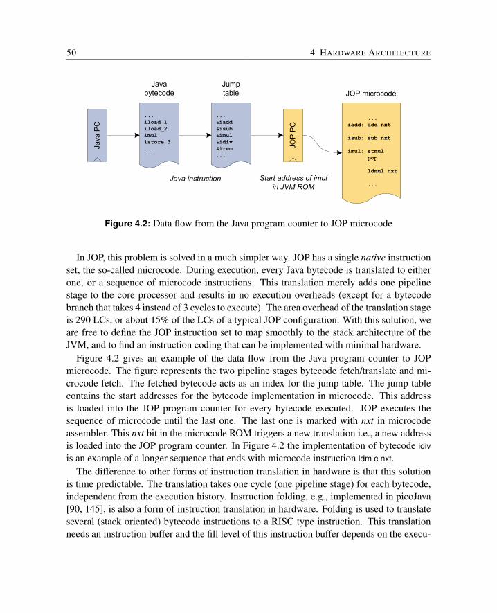
50 4 HARDWARE ARCHITECTURE
Java
PC
JOP
PC
...iload_1iload_2imulistore_3...
...iadd: add nxt
isub: sub nxt
imul: stmulpop...ldmul nxt
...
...&iadd&isub&imul&idiv&irem...
Javabytecode
Jumptable JOP microcode
Java instruction Start address of imulin JVM ROM
Figure 4.2: Data flow from the Java program counter to JOP microcode
In JOP, this problem is solved in a much simpler way. JOP has a single native instructionset, the so-called microcode. During execution, every Java bytecode is translated to eitherone, or a sequence of microcode instructions. This translation merely adds one pipelinestage to the core processor and results in no execution overheads (except for a bytecodebranch that takes 4 instead of 3 cycles to execute). The area overhead of the translation stageis 290 LCs, or about 15% of the LCs of a typical JOP configuration. With this solution, weare free to define the JOP instruction set to map smoothly to the stack architecture of theJVM, and to find an instruction coding that can be implemented with minimal hardware.
Figure 4.2 gives an example of the data flow from the Java program counter to JOPmicrocode. The figure represents the two pipeline stages bytecode fetch/translate and mi-crocode fetch. The fetched bytecode acts as an index for the jump table. The jump tablecontains the start addresses for the bytecode implementation in microcode. This addressis loaded into the JOP program counter for every bytecode executed. JOP executes thesequence of microcode until the last one. The last one is marked with nxt in microcodeassembler. This nxt bit in the microcode ROM triggers a new translation i.e., a new addressis loaded into the JOP program counter. In Figure 4.2 the implementation of bytecode idivis an example of a longer sequence that ends with microcode instruction ldm c nxt.
The difference to other forms of instruction translation in hardware is that this solutionis time predictable. The translation takes one cycle (one pipeline stage) for each bytecode,independent from the execution history. Instruction folding, e.g., implemented in picoJava[90, 145], is also a form of instruction translation in hardware. Folding is used to translateseveral (stack oriented) bytecode instructions to a RISC type instruction. This translationneeds an instruction buffer and the fill level of this instruction buffer depends on the execu-
4.2 MICROCODE 51
tion history. The length of this history that has to be considered for analysis is not bounded.Therefore this form of instruction translation is not exactly time predictable.
4.2.2 Compact Microcode
For the JVM to be implemented efficiently, the microcode has to fit to the Java bytecode.Since the JVM is a stack machine, the microcode is also stack-oriented. However, the JVMis not a pure stack machine. Method parameters and local variables are defined as locals.These locals can reside in a stack frame of the method and are accessed with an offsetrelative to the start of this locals area.
Additional local variables (16) are available at the microcode level. These variables serveas scratch variables, like registers in a conventional CPU. Furthermore, the constant poolpointer (cp), the method pointer (mp), and pointers to the method tables of JVM.java andJVMHelp.java are stored in these variables. The 16 variables are located in the on-chip stackmemory. However, arithmetic and logic operations are performed on the stack.
Some bytecodes, such as ALU operations and the short form access to locals, are directlyimplemented by an equivalent microcode instruction (with a different encoding). Addi-tional instructions are available to access internal registers, main memory and I/O devices.A relative conditional branch (zero/non zero of TOS) performs control flow decisions atthe microcode level. For optimum use of the available memory resources, all instructionsare 8 bits long. There are no variable-length instructions and every instruction, with theexception of wait, is executed in a single cycle. To keep the instruction set this dense, thefollowing concept is applied: immediate values and branch offsets are addressed throughone indirection. The instruction just contains an index for the constants.
Two types of operands, immediate values and branch distances, normally force an in-struction set to be longer than 8 bits. The instruction set is either expanded to 16 or 32 bits,as in typical RISC processors, or allowed to be of variable length at byte boundaries. A firstimplementation of the JVM with a 16-bit instruction set showed that only a small numberof different constants are necessary for immediate values and relative branch distances.
In the current realization of JOP, the different immediate values are collected while themicrocode is being assembled and are put into the initialization file for the on-chip memory.These constants are accessed indirectly in the same way as the local variables. They aresimilar to initialized variables, apart from the fact that there are no operations to changetheir value during runtime, which would serve no purpose and would waste instructioncodes. The microcode local variables, the microcode constants and the stack share the sameon-chip memory. Using a single memory block simplifies the multiplexer in the executionstage.
52 4 HARDWARE ARCHITECTURE
A similar solution is used for branch distances. The assembler generates a VHDL filewith a table for all found branch constants. This table is indexed using instruction bits dur-ing runtime. These indirections during runtime make it possible to retain an 8-bit instructionset, and provide 16 different immediate values and 32 different branch constants. For a gen-eral purpose instruction set, these indirections would impose too many restrictions. As themicrocode only implements the JVM, this solution is a viable option.
To simplify the logic for instruction decoding, the instruction coding is carefully chosen.For example, one bit in the instruction specifies whether the instruction will incrementor decrement the stack pointer. The offset to access the locals is directly encoded in theinstruction. This is not the case for the original encoding of the equivalent bytecodes (e.g.iload 0 is 0x1a and iload 1 is 0x1b). Whenever a multiplexer depends on an instruction,the selection is directly encoded in the instruction.
4.2.3 Instruction Set
JOP implements 54 different microcode instructions. These instructions are encoded in 8bits. With the addition of the nxt and opd bits in every instruction, the effective instructionlength is 10 bits.
Bytecode equivalent: These instructions are direct implementations of bytecodes and re-sult in one cycle execution time for the bytecode (except st and ld): pop, and, or, xor,add, sub, st<n>, st, ushr, shl, shr, nop, ld<n>, ld, dup
Local memory access: The first 16 words in the internal stack memory are reserved forinternal variables. The next 16 words contain constants. These memory locations areaccessed using the following instructions: stm, stmi, ldm, ldmi, ldi
Register manipulation: The stack pointer, the variable pointer and the Java programcounter are loaded or stored with: stvp, stjpc, stsp, ldvp, ldjpc, ldsp, star
Bytecode operand: The operand is loaded from the bytecode RAM, converted to a 32-bitword and pushed on the stack with: ld opd 8s, ld opd 8u, ld opd 16s, ld opd 16u
External memory access: The autonomous memory subsystem and the I/O subsystem areaccessed by using the following instructions: stmra, stmwa, stmwd, wait, ldmrd, stbcrd,ldbcstart, stald, stast, stgf, stpf, stcp
Multiplier: The multiplier is accessed with: stmul, ldmul
Microcode branches: Two conditional branches in microcode are available: bz, bnz
4.2 MICROCODE 53
iadd: add nxt // 1 to 1 mapping
// a and b are scratch variables for the// JVM code.swap: stm a // save TOS in variable a
stm b // save TOS−1 in variable bldm a // push a on stackldm b nxt // push b on stack and fetch next bytecode
Listing 4.1: Implementation of iadd and swap
Bytecode branch: All 17 bytecode branch instructions are mapped to one instruction: jbr
A detailed description of the microcode instructions can be found in Appendix C.
4.2.4 Bytecode Example
The example in Figure 4.1 shows the implementation of a single cycle bytecode and aninfrequent bytecode as a sequence of JOP instructions. The suffix nxt marks the last in-struction of the microcode sequence. In this example, the iadd bytecode is mapped to theequivalent add microcode and executed in a single cycle, whereas swap takes four cycles toexecute, and after the last instruction (ldm b nxt), the first instruction for the next bytecode isexecuted. The scratch variables, as shown in the second example, are stored in the on-chipmemory that is shared with the stack cache.
Some bytecodes are followed by operands of between one and three bytes in length (ex-cept lookupswitch and tableswitch). Due to pipelining, the first operand byte that follows thebytecode instruction is available when the first microcode instruction enters the executionstage. If this is a one-byte long operand, it is ready to be accessed. The increment of theJava program counter after the read of an operand byte is coded in the JOP instruction (anopd bit similar to the nxt bit).
In Listing 4.2, the implementation of sipush is shown. The bytecode is followed by atwo-byte operand. Since the access to bytecode memory is only one4 byte per cycle, opdand nxt are not allowed at the same time. This implies a minimum execution time of n+1cycles for a bytecode with n operand bytes.
4The decision is to avoid buffers that would introduce time dependencies over bytecode boundaries.
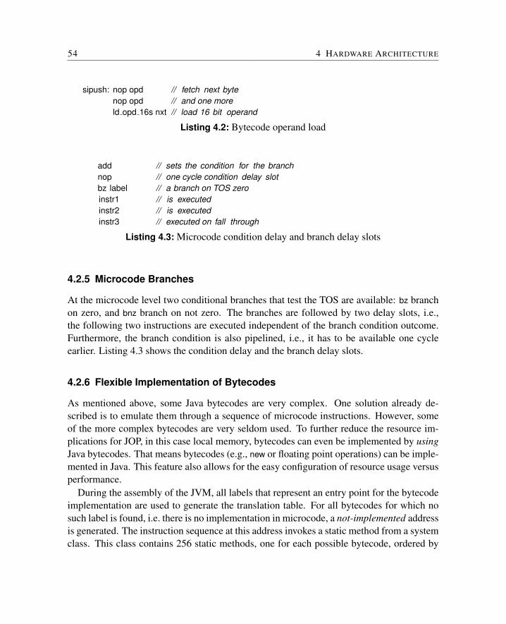
54 4 HARDWARE ARCHITECTURE
sipush: nop opd // fetch next bytenop opd // and one moreld opd 16s nxt // load 16 bit operand
Listing 4.2: Bytecode operand load
add // sets the condition for the branchnop // one cycle condition delay slotbz label // a branch on TOS zeroinstr1 // is executedinstr2 // is executedinstr3 // executed on fall through
Listing 4.3: Microcode condition delay and branch delay slots
4.2.5 Microcode Branches
At the microcode level two conditional branches that test the TOS are available: bz branchon zero, and bnz branch on not zero. The branches are followed by two delay slots, i.e.,the following two instructions are executed independent of the branch condition outcome.Furthermore, the branch condition is also pipelined, i.e., it has to be available one cycleearlier. Listing 4.3 shows the condition delay and the branch delay slots.
4.2.6 Flexible Implementation of Bytecodes
As mentioned above, some Java bytecodes are very complex. One solution already de-scribed is to emulate them through a sequence of microcode instructions. However, someof the more complex bytecodes are very seldom used. To further reduce the resource im-plications for JOP, in this case local memory, bytecodes can even be implemented by usingJava bytecodes. That means bytecodes (e.g., new or floating point operations) can be imple-mented in Java. This feature also allows for the easy configuration of resource usage versusperformance.
During the assembly of the JVM, all labels that represent an entry point for the bytecodeimplementation are used to generate the translation table. For all bytecodes for which nosuch label is found, i.e. there is no implementation in microcode, a not-implemented addressis generated. The instruction sequence at this address invokes a static method from a systemclass. This class contains 256 static methods, one for each possible bytecode, ordered by
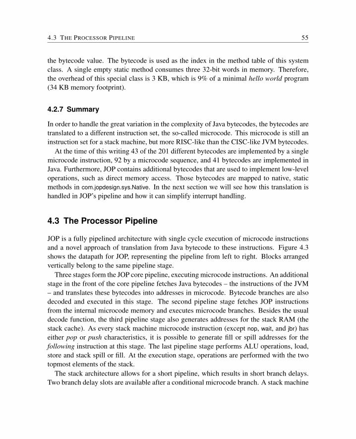
4.3 THE PROCESSOR PIPELINE 55
the bytecode value. The bytecode is used as the index in the method table of this systemclass. A single empty static method consumes three 32-bit words in memory. Therefore,the overhead of this special class is 3 KB, which is 9% of a minimal hello world program(34 KB memory footprint).
4.2.7 Summary
In order to handle the great variation in the complexity of Java bytecodes, the bytecodes aretranslated to a different instruction set, the so-called microcode. This microcode is still aninstruction set for a stack machine, but more RISC-like than the CISC-like JVM bytecodes.
At the time of this writing 43 of the 201 different bytecodes are implemented by a singlemicrocode instruction, 92 by a microcode sequence, and 41 bytecodes are implemented inJava. Furthermore, JOP contains additional bytecodes that are used to implement low-leveloperations, such as direct memory access. Those bytecodes are mapped to native, staticmethods in com.jopdesign.sys.Native. In the next section we will see how this translation ishandled in JOP’s pipeline and how it can simplify interrupt handling.
4.3 The Processor Pipeline
JOP is a fully pipelined architecture with single cycle execution of microcode instructionsand a novel approach of translation from Java bytecode to these instructions. Figure 4.3shows the datapath for JOP, representing the pipeline from left to right. Blocks arrangedvertically belong to the same pipeline stage.
Three stages form the JOP core pipeline, executing microcode instructions. An additionalstage in the front of the core pipeline fetches Java bytecodes – the instructions of the JVM– and translates these bytecodes into addresses in microcode. Bytecode branches are alsodecoded and executed in this stage. The second pipeline stage fetches JOP instructionsfrom the internal microcode memory and executes microcode branches. Besides the usualdecode function, the third pipeline stage also generates addresses for the stack RAM (thestack cache). As every stack machine microcode instruction (except nop, wait, and jbr) haseither pop or push characteristics, it is possible to generate fill or spill addresses for thefollowing instruction at this stage. The last pipeline stage performs ALU operations, load,store and stack spill or fill. At the execution stage, operations are performed with the twotopmost elements of the stack.
The stack architecture allows for a short pipeline, which results in short branch delays.Two branch delay slots are available after a conditional microcode branch. A stack machine
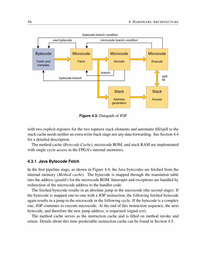
56 4 HARDWARE ARCHITECTURE
Bytecode
Fetch and translate
Microcode
Fetch
Microcode
Decode
Microcode
Execute
Stack
Addressgeneration
Stack
Access
next bytecode
bytecode branch condition
microcode branch condition
branch
bytecode branch spill,fill
Figure 4.3: Datapath of JOP
with two explicit registers for the two topmost stack elements and automatic fill/spill to thestack cache needs neither an extra write-back stage nor any data forwarding. See Section 4.4for a detailed description.
The method cache (Bytecode Cache), microcode ROM, and stack RAM are implementedwith single cycle access in the FPGA’s internal memories.
4.3.1 Java Bytecode Fetch
In the first pipeline stage, as shown in Figure 4.4, the Java bytecodes are fetched from theinternal memory (Method cache). The bytecode is mapped through the translation tableinto the address (jpaddr) for the microcode ROM. Interrupts and exceptions are handled byredirection of the microcode address to the handler code.
The fetched bytecode results in an absolute jump in the microcode (the second stage). Ifthe bytecode is mapped one-to-one with a JOP instruction, the following fetched bytecodeagain results in a jump in the microcode in the following cycle. If the bytecode is a complexone, JOP continues to execute microcode. At the end of this instruction sequence, the nextbytecode, and therefore the new jump address, is requested (signal nxt).
The method cache serves as the instruction cache and is filled on method invoke andreturn. Details about this time-predictable instruction cache can be found in Section 4.5.
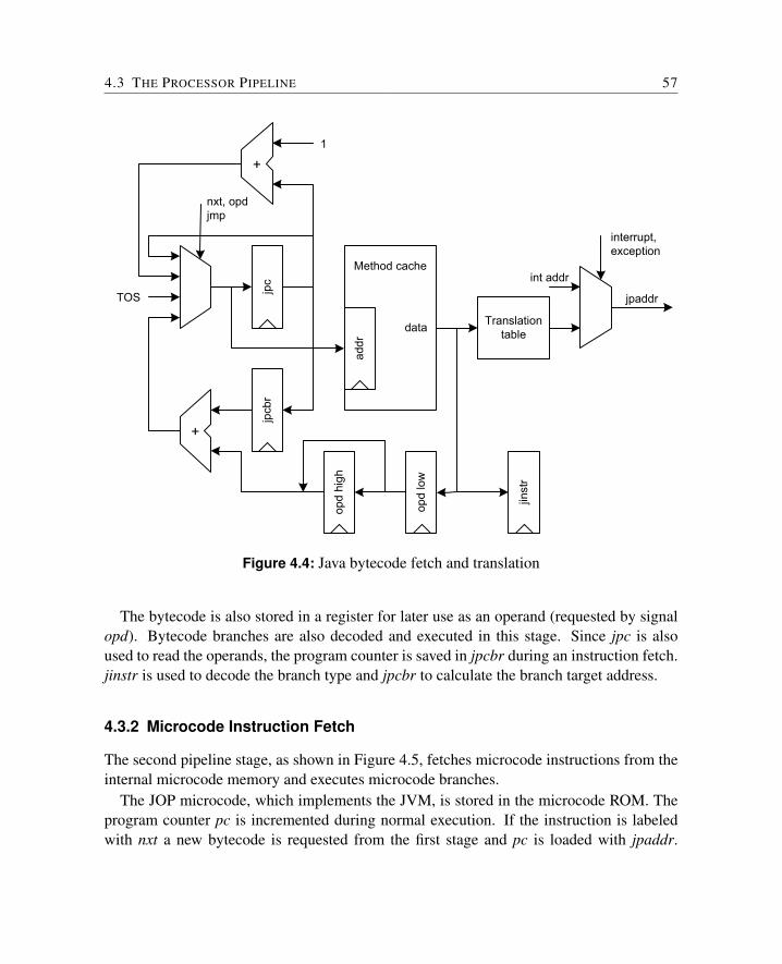
4.3 THE PROCESSOR PIPELINE 57
jpc
jpcb
rMethod cache
addr
data
1
nxt, opdjmp
TOS
opd
high
opd
low
jinst
r
Translationtable
jpaddr
interrupt,exception
int addr
+
+
Figure 4.4: Java bytecode fetch and translation
The bytecode is also stored in a register for later use as an operand (requested by signalopd). Bytecode branches are also decoded and executed in this stage. Since jpc is alsoused to read the operands, the program counter is saved in jpcbr during an instruction fetch.jinstr is used to decode the branch type and jpcbr to calculate the branch target address.
4.3.2 Microcode Instruction Fetch
The second pipeline stage, as shown in Figure 4.5, fetches microcode instructions from theinternal microcode memory and executes microcode branches.
The JOP microcode, which implements the JVM, is stored in the microcode ROM. Theprogram counter pc is incremented during normal execution. If the instruction is labeledwith nxt a new bytecode is requested from the first stage and pc is loaded with jpaddr.
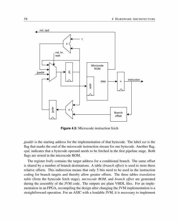
58 4 HARDWARE ARCHITECTURE
pc
jpcb
r
MicrocodeROM
addr
data
1
nxt, br,wait
jpaddr
ir
+
+Branchoffset
instruction
nxt, opd
Figure 4.5: Microcode instruction fetch
jpaddr is the starting address for the implementation of that bytecode. The label nxt is theflag that marks the end of the microcode instruction stream for one bytecode. Another flag,opd, indicates that a bytecode operand needs to be fetched in the first pipeline stage. Bothflags are stored in the microcode ROM.
The register brdly contains the target address for a conditional branch. The same offsetis shared by a number of branch destinations. A table (branch offset) is used to store theserelative offsets. This indirection means that only 5 bits need to be used in the instructioncoding for branch targets and thereby allow greater offsets. The three tables translationtable (from the bytecode fetch stage), microcode ROM, and branch offset are generatedduring the assembly of the JVM code. The outputs are plain VHDL files. For an imple-mentation in an FPGA, recompiling the design after changing the JVM implementation is astraightforward operation. For an ASIC with a loadable JVM, it is necessary to implement
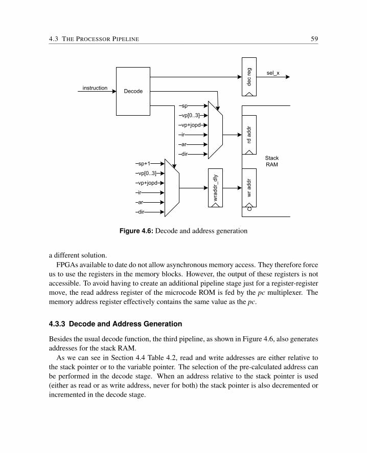
4.3 THE PROCESSOR PIPELINE 59
Decode
sp
vp[0..3]
vp+jopd
ir
ar
dir
sp+1
vp[0..3]
vp+jopd
ir
ar
dirw
radd
r_dl
y
instruction
dec
reg
rd a
ddr
wr a
ddr
sel_x
StackRAM
Figure 4.6: Decode and address generation
a different solution.FPGAs available to date do not allow asynchronous memory access. They therefore force
us to use the registers in the memory blocks. However, the output of these registers is notaccessible. To avoid having to create an additional pipeline stage just for a register-registermove, the read address register of the microcode ROM is fed by the pc multiplexer. Thememory address register effectively contains the same value as the pc.
4.3.3 Decode and Address Generation
Besides the usual decode function, the third pipeline, as shown in Figure 4.6, also generatesaddresses for the stack RAM.
As we can see in Section 4.4 Table 4.2, read and write addresses are either relative tothe stack pointer or to the variable pointer. The selection of the pre-calculated address canbe performed in the decode stage. When an address relative to the stack pointer is used(either as read or as write address, never for both) the stack pointer is also decremented orincremented in the decode stage.
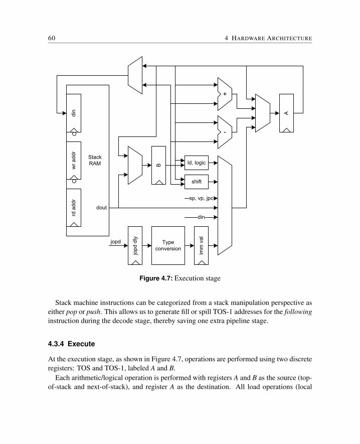
60 4 HARDWARE ARCHITECTURE
StackRAM
din
wr a
ddr
rd a
ddr
ld, logic
shift
imm
val
sp, vp, jpc
dout
din
B
Typeconversion
jopd
dlyjopd
-
+
AFigure 4.7: Execution stage
Stack machine instructions can be categorized from a stack manipulation perspective aseither pop or push. This allows us to generate fill or spill TOS-1 addresses for the followinginstruction during the decode stage, thereby saving one extra pipeline stage.
4.3.4 Execute
At the execution stage, as shown in Figure 4.7, operations are performed using two discreteregisters: TOS and TOS-1, labeled A and B.
Each arithmetic/logical operation is performed with registers A and B as the source (top-of-stack and next-of-stack), and register A as the destination. All load operations (local
4.3 THE PROCESSOR PIPELINE 61
variables, internal register, external memory and periphery) result in a value being loadedinto register A. There is no need for a write-back pipeline stage. Register A is also thesource for the store operations. Register B is never accessed directly. It is read as animplicit operand or for stack spill on push instructions. It is written during the stack spillwith the content of the stack RAM or the stack fill with the content of register A.
Beside the Java stack, the stack RAM also contains microcode variables and constants.This resource-sharing arrangement not only reduces the number of memory blocks neededfor the processor, but also the number of data paths to and from the register A.
The inverted clock on data-in and on the write address register of the stack RAM is usedto perform the RAM write in the same cycle as the execute operation.
A stack machine with two explicit registers for the two topmost stack elements and auto-matic fill/spill needs neither an extra write-back stage nor any data forwarding. Details ofthis two-level stack architecture are described in Section 4.4.
4.3.5 Interrupt Logic
Interrupts and (precise) exceptions are considered hard to implement in a pipelined proces-sor [62], meaning implementation tends to be complex (and therefore resource consuming).In JOP, the bytecode-microcode translation is used cleverly to avoid having to handle inter-rupts and exceptions (e.g., stack overflow) in the core pipeline.
Interrupts are implemented as special bytecodes. These bytecodes are inserted by thehardware in the Java instruction stream. When an interrupt is pending and the next fetchedbyte from the bytecode cache is an instruction (as indicated by the nxt bit in the microcode),the associated special bytecode is used instead of the instruction from the bytecode cache.The result is that interrupts are accepted at bytecode boundaries. The worst-case preemp-tion delay is the execution time of the slowest bytecode that is implemented in microcode.Bytecodes that are implemented in Java (see Section 4.2.6) can be interrupted.
The implementation of interrupts at the bytecode-microcode mapping stage keeps inter-rupts transparent in the core pipeline and avoids complex logic. Interrupt handlers can beimplemented in the same way as standard bytecodes are implemented i.e. in microcode orJava.
This special bytecode can result in a call of a JVM internal method in the context of theinterrupted thread. This mechanism implicitly stores almost the complete context of thecurrent active thread on the stack. This feature is used to implement the preemptive, fixedpriority real-time scheduler in Java [118].
The main source for an interrupt is the µs accurate timer interrupt used by the real-timescheduler. I/O device interrupts can also be connected to the interrupt controller. Hardware
62 4 HARDWARE ARCHITECTURE
generated exceptions, such as stack overflow or array bounds checks, generate a systeminterrupt. The exception reason can be found in a register.
4.3.6 Summary
In this section, we have analyzed JOP’s pipeline. The core of the stack machine constitutesa three-stage pipeline. In the following section, we will see that this organization is anoptimal solution for the stack access pattern of the JVM.
An additional pipeline stage in front of this core pipeline stage performs bytecode fetchand the translation to microcode. This organization has zero overheads for more complexbytecodes and results in the short pipeline that is necessary for any processor without branchprediction. This additional translation stage also presents an elegant way of incorporatinginterrupts virtually for free.
4.4 THE STACK CACHE 63
4.4 The Stack Cache
The Java programming language defines not only the language but also a binary represen-tation of the program and an abstract machine, the JVM, to execute this binary. The JVM issimilar to the Forth abstract machine in that it is also a stack machine. However, the usageof the stack differs from Forth in such a way that a Forth processor is not an ideal hardwareplatform to execute Java programs.
In this section, the stack usage in the JVM is analyzed. We will see that, besides theaccess to the top elements of the stack, an additional access path to an arbitrary element ofthe stack is necessary for an efficient implementation of the JVM.
As the stack is a heavily accessed memory region, the stack – or part of it – has to beplaced in the upper level of the memory hierarchy. This part of the stack is referred to as astack cache. We will show that the JVM does not need a full three-port access to the stack.This allows for a simple and elegant design of the stack cache for a Java processor.
Other stack cache implementations use three port memories (e.g., in Komodo [76]) ordiscrete register files (e.g., picoJava [145] and the aJile JEMCore [55]). The comparison ofthe JOP stack organization with the other two approaches can be found in [121].
4.4.1 Java Computing Model
The JVM is not a pure stack machine in the sense of, for instance, the stack model in Forth.The JVM operates on a LIFO stack as its operand stack. The JVM supplies instructions toload values on the operand stack, and other instructions take their operands from the stack,operate on them and push the result back onto the stack. For example, the iadd instructionpops two values from the stack and pushes the result back onto the stack. These instruc-tions are the stack machine’s typical zero-address instructions. The maximum depth of thisoperand stack is known at compile time. In typical Java programs, the maximum depth isvery small. To illustrate the operation notation of the JVM, Table 4.1 shows the evaluationof an expression for a stack machine notation and the JVM bytecodes. Instruction iload nloads an integer value from a local variable at position n and pushes the value on TOS.
The JVM contains another memory area for method local data. This area is known aslocal variables. Primitive type values, such as integer and float, and references to objects arestored in these local variables. Arrays and objects cannot be allocated in a local variable, asin C/C++. They have to be placed on the heap. Different instructions transfer data betweenthe operand stack and the local variables. Access to the first four elements is optimizedwith dedicated single byte instructions, while up to 256 local variables are accessed with atwo-byte instruction and, with the wide modifier, the area can contain up to 65536 values.
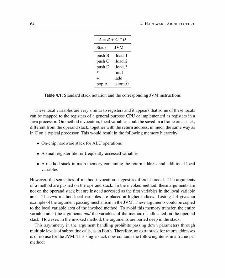
64 4 HARDWARE ARCHITECTURE
A = B + C * D
Stack JVM
push B iload 1push C iload 2push D iload 3* imul+ iaddpop A istore 0
Table 4.1: Standard stack notation and the corresponding JVM instructions
These local variables are very similar to registers and it appears that some of these localscan be mapped to the registers of a general purpose CPU or implemented as registers in aJava processor. On method invocation, local variables could be saved in a frame on a stack,different from the operand stack, together with the return address, in much the same way asin C on a typical processor. This would result in the following memory hierarchy:
• On-chip hardware stack for ALU operations
• A small register file for frequently-accessed variables
• A method stack in main memory containing the return address and additional localvariables
However, the semantics of method invocation suggest a different model. The argumentsof a method are pushed on the operand stack. In the invoked method, these arguments arenot on the operand stack but are instead accessed as the first variables in the local variablearea. The real method local variables are placed at higher indices. Listing 4.4 gives anexample of the argument passing mechanism in the JVM. These arguments could be copiedto the local variable area of the invoked method. To avoid this memory transfer, the entirevariable area (the arguments and the variables of the method) is allocated on the operandstack. However, in the invoked method, the arguments are buried deep in the stack.
This asymmetry in the argument handling prohibits passing down parameters throughmultiple levels of subroutine calls, as in Forth. Therefore, an extra stack for return addressesis of no use for the JVM. This single stack now contains the following items in a frame permethod:
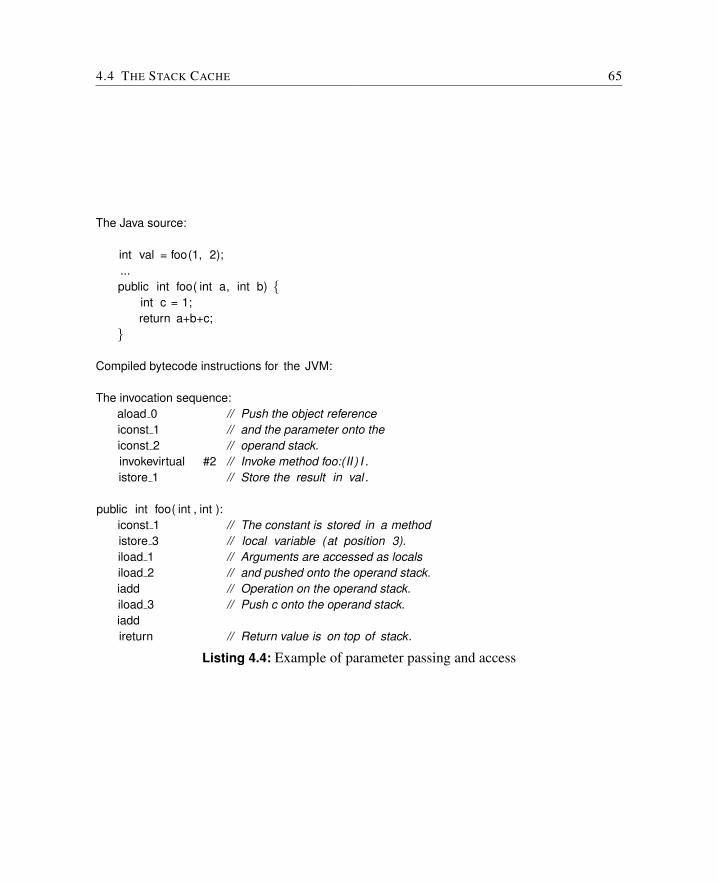
4.4 THE STACK CACHE 65
The Java source:
int val = foo(1, 2);...public int foo( int a, int b) {
int c = 1;return a+b+c;
}
Compiled bytecode instructions for the JVM:
The invocation sequence:aload 0 // Push the object referenceiconst 1 // and the parameter onto theiconst 2 // operand stack.invokevirtual #2 // Invoke method foo:(II ) I .istore 1 // Store the result in val .
public int foo( int , int ):iconst 1 // The constant is stored in a methodistore 3 // local variable (at position 3).iload 1 // Arguments are accessed as localsiload 2 // and pushed onto the operand stack.iadd // Operation on the operand stack.iload 3 // Push c onto the operand stack.iaddireturn // Return value is on top of stack.
Listing 4.4: Example of parameter passing and access
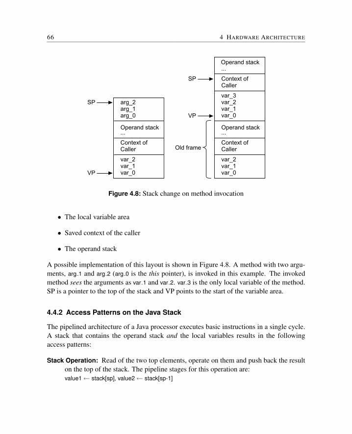
66 4 HARDWARE ARCHITECTURE
var_2var_1var_0
Operand stack
arg_2arg_1arg_0
var_2var_1var_0
Context ofCaller
Operand stack
var_3var_2var_1var_0
Context ofCaller
VP
SP
VP
Old frame
SP
Context ofCaller
Operand stack
... ...
...
Figure 4.8: Stack change on method invocation
• The local variable area
• Saved context of the caller
• The operand stack
A possible implementation of this layout is shown in Figure 4.8. A method with two argu-ments, arg 1 and arg 2 (arg 0 is the this pointer), is invoked in this example. The invokedmethod sees the arguments as var 1 and var 2. var 3 is the only local variable of the method.SP is a pointer to the top of the stack and VP points to the start of the variable area.
4.4.2 Access Patterns on the Java Stack
The pipelined architecture of a Java processor executes basic instructions in a single cycle.A stack that contains the operand stack and the local variables results in the followingaccess patterns:
Stack Operation: Read of the two top elements, operate on them and push back the resulton the top of the stack. The pipeline stages for this operation are:value1← stack[sp], value2← stack[sp-1]
4.4 THE STACK CACHE 67
result← value1 op value2, sp← sp-1stack[sp]← result
Variable Load: Read a data element deeper down in the stack, relative to a variable baseaddress pointer (VP), and push this data on the top of the stack. This operation needstwo pipeline stages:value← stack[vp+offset], sp← sp+1stack[sp]← value
Variable Store: Pop the top element of the stack and write it in the variable relative to thevariable base address:value← stack[sp]stack[vp+offset]← value, sp← sp-1
For pipelined execution of these operations, a three-port memory or register file (two readports and one write port) would be necessary.
In following section, we will discuss access patterns of the JVM and their implication onthe functional units of the pipeline. A fast and small architecture for the stack cache of aJava processor is described.
4.4.3 JVM Stack Access Revised
If we analyze the JVM’s access patterns to the stack in more detail, we can see that a two-port read is only performed with the two top elements of the stack. All other operationswith elements deeper in the stack, local variables load and store, only need one read port.If we only implement the two top elements of the stack in registers, we can use a standardon-chip RAM with one read and one write port.
We will show that all operations can be performed with this configuration. Let A be thetop-of-stack, B the element below top-of-stack. The memory that serves as the second levelcache is represented by the array sm. Two indices in this array are used: p points to thelogical third element of the stack and changes as the stack grows or shrinks, v points to thebase of the local variables area in the stack and n is the address offset of a variable. op is a
68 4 HARDWARE ARCHITECTURE
two operand stack operation with a single result (i.e. a typical ALU operation).
Case 1: ALU operationA← A op BB← sm[p]p← p – 1The two operands are provided by the two top level registers. A single read accessfrom sm is necessary to fill B with a new value.
Case 2: Variable load (Push)sm[p+1]← BB← AA← sm[v+n]p← p + 1One read access from sm is necessary for the variable read. The former TOS valuemoves down to B and the data previously in B is written to sm.
Case 3: Variable store (Pop)sm[v+n]← AA← BB← sm[p]p← p - 1The TOS value is written to sm. A is filled with B and B is filled in an identicalmanner to Case 1, needing a single read access from sm.
We can see that all three basic operations can be performed with a stack memory with oneread and one write port. Assuming a memory is used that can handle concurrent read andwrite access, there is no structural access conflict between A, B and sm. That means that alloperations can be performed concurrently in a single cycle.
As we can see in Figure 4.8 the operand stack and the local variables area are distinctregions of the stack. A concurrent read from and write to the stack is only performed on avariable load or store. When the read is from the local variables area the write goes to theoperand area; a read from the operand area is concurrent with a write to the local variablesarea. Therefore there is no concurrent read and write to the same location in sm. Thereis no constraint on the read-during-write behavior of the memory (old data, undefined ornew data), which simplifies the memory design. In a design where read and write-backare located in different pipeline stages, as in the architectures described above, either the
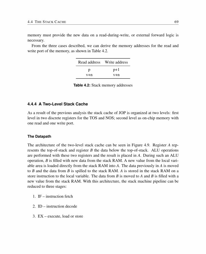
4.4 THE STACK CACHE 69
memory must provide the new data on a read-during-write, or external forward logic isnecessary.
From the three cases described, we can derive the memory addresses for the read andwrite port of the memory, as shown in Table 4.2.
Read address Write address
p p+1v+n v+n
Table 4.2: Stack memory addresses
4.4.4 A Two-Level Stack Cache
As a result of the previous analysis the stack cache of JOP is organized at two levels: firstlevel in two discrete registers for the TOS and NOS; second level as on-chip memory withone read and one write port.
The Datapath
The architecture of the two-level stack cache can be seen in Figure 4.9. Register A rep-resents the top-of-stack and register B the data below the top-of-stack. ALU operationsare performed with these two registers and the result is placed in A. During such an ALUoperation, B is filled with new data from the stack RAM. A new value from the local vari-able area is loaded directly from the stack RAM into A. The data previously in A is movedto B and the data from B is spilled to the stack RAM. A is stored in the stack RAM on astore instruction to the local variable. The data from B is moved to A and B is filled with anew value from the stack RAM. With this architecture, the stack machine pipeline can bereduced to three stages:
1. IF – instruction fetch
2. ID – instruction decode
3. EX – execute, load or store
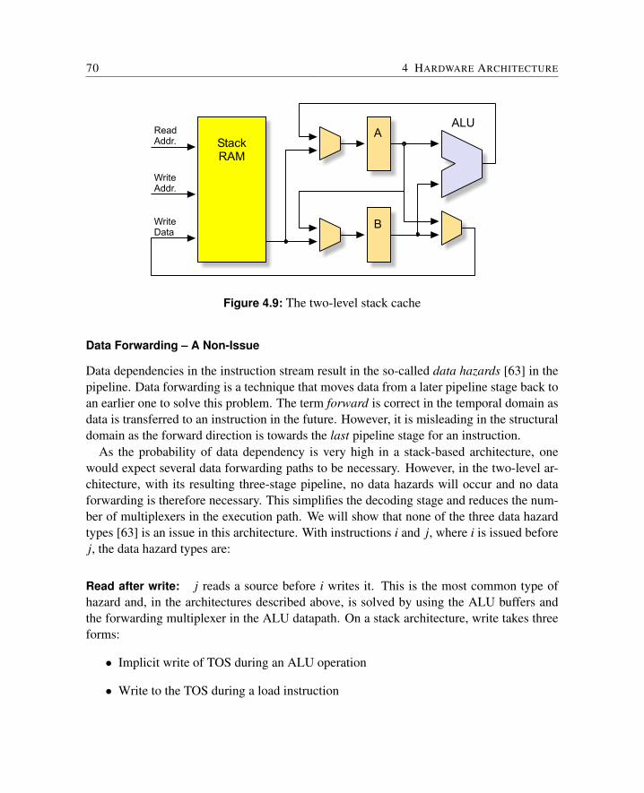
70 4 HARDWARE ARCHITECTURE
ALUReadAddr.
WriteAddr.
WriteData
StackRAM
A
B
Figure 4.9: The two-level stack cache
Data Forwarding – A Non-Issue
Data dependencies in the instruction stream result in the so-called data hazards [63] in thepipeline. Data forwarding is a technique that moves data from a later pipeline stage back toan earlier one to solve this problem. The term forward is correct in the temporal domain asdata is transferred to an instruction in the future. However, it is misleading in the structuraldomain as the forward direction is towards the last pipeline stage for an instruction.
As the probability of data dependency is very high in a stack-based architecture, onewould expect several data forwarding paths to be necessary. However, in the two-level ar-chitecture, with its resulting three-stage pipeline, no data hazards will occur and no dataforwarding is therefore necessary. This simplifies the decoding stage and reduces the num-ber of multiplexers in the execution path. We will show that none of the three data hazardtypes [63] is an issue in this architecture. With instructions i and j, where i is issued beforej, the data hazard types are:
Read after write: j reads a source before i writes it. This is the most common type ofhazard and, in the architectures described above, is solved by using the ALU buffers andthe forwarding multiplexer in the ALU datapath. On a stack architecture, write takes threeforms:
• Implicit write of TOS during an ALU operation
• Write to the TOS during a load instruction
4.4 THE STACK CACHE 71
• Write to an arbitrary entry of the stack with a store instruction
A read also occurs in three different forms:
• Read two top values from the stack for an ALU operation
• Read TOS for a store instruction
• Read an arbitrary entry of the stack with the load instruction
With the two top elements of the stack as discrete registers, these values are read, operatedon and written back in the same cycle. No read that depends on TOS or TOS-1 suffersfrom a data hazard. Read and write access to a local variable is also performed in the samepipeline stage. Thus, the read after write order is not affected. However, there is also anadditional hidden read and write: the fill and spill of register B:
B fill: B is written during an ALU operation and on a variable store. During an ALUoperation, the operands are the values from A and the old value from B. The newvalue for B is read from the stack memory and does not depend on the new valueof A. During a variable store operation, A is written to the stack memory and doesnot depend on B. The new value for B is also read from the stack memory andit is not obvious that this value does not depend on the written value. However, thevariable area and the operand stack are distinct areas in the stack (this changes only onmethod invocation and return), guaranteeing that concurrent read/write access doesnot produce a data hazard.
B spill: B is read on a load operation. The new value of B is the old value of A and doesnot therefore depend on the stack memory read. B is written to the stack. For the readvalue from the stack memory that goes to A, the argument concerning the distinctstack areas in the case of B fill described above still applies.
Write after read: j writes a destination before it is read by i. This cannot take place as allreads and writes are performed in the same pipeline stage keeping the instruction order.
Write after write: j writes an operand before it is written by i. This hazard is not presentin this architecture as all writes are performed in the same pipeline stage.
72 4 HARDWARE ARCHITECTURE
4.4.5 Summary
In this section, the stack architecture of the JVM was analyzed. We have seen that the JVMis different from the classical stack architecture. The JVM uses the stack both as an operandstack and as the storage place for local variables. Local variables are placed in the stack ata deeper position. To load and store these variables, an access path to an arbitrary positionin the stack is necessary. As the stack is the most frequently accessed memory area in theJVM, caching of this memory is mandatory for a high-performing Java processor.
A common solution, found in a number of different Java processors, is to implementthis stack cache as a standard three-port register file with additional support to address thisregister file in a stack like manner. The architectures presented above differ in the realizationof the register file: as a discrete register or in on-chip memory. Implementing the stackcache as discrete registers is very expensive. A three-port memory is also an expensiveoption for an ASIC and unusual in an FPGA. It can be emulated by two memories with asingle read and write port. However, this solution also doubles the amount of memory.
Detailed analysis of the access patterns to the stack showed that only the two top elementsof the stack are accessed in a single cycle. Given this fact, the architecture uses registers tocache only the two top elements of the stack. The next level of the stack cache is providedby a simple on-chip memory. The memory automatically spills and fills the second register.Implementing the two top elements of the stack as fixed registers, instead of elements thatare indexed by a stack pointer, also greatly simplifies the overall pipeline.
4.5 THE METHOD CACHE 73
4.5 The Method Cache
Worst-case execution time (WCET) analysis [109] of real-time programs is essential forany schedulability analysis. To provide a low WCET value, a good processor model is nec-essary. However, caches for the instructions and data is a classic example of the paradigmMake the common case fast, which complicates WCET analysis. Avoiding or ignoring thisfeature in real-time systems, due to its unpredictable behavior, results in a very pessimisticWCET value. Plenty of effort has gone into research into integrating the instruction cachein the timing analysis of tasks [11, 60, 81] and the influence of the cache on task preemption[78, 31]. The influence of different cache architectures on WCET analysis is described in[61].
We will tackle this problem from the architectural side – an instruction cache organizationin which simpler and more accurate WCET analysis is more important than average caseperformance.
In this section, we will explore the method cache, as it is implemented in JOP, with anovel replacement policy. In Java bytecode only relative branches exist, and a method istherefore only left when a return instruction has been executed.5 It has been observed thatmethods are typically short (see [123]) in Java applications. These properties are utilizedby a cache architecture that stores complete methods. A complete method is loaded intothe cache on both invocation and return. This cache fill strategy lumps all cache missestogether and is very simple to analyze.
The method cache was first presented in [120] and is now also used by the Java processorSHAP [102]. Furthermore, the idea has been adapted for a processor that executes compiledC programs [86].
4.5.1 Method Cache Architecture
In this section, we will develop a solution for a time-predictable instruction cache. TypicalJava programs consist of short methods. There are no branches out of the method and allbranches inside are relative. In the described architecture, the full code of a method isloaded into the cache before execution. The cache is filled on invocations and returns. Thismeans that all cache fills are lumped together with a known execution time. The full loadedmethod and relative addressing inside a method also result in a simpler cache. Tag memoryand address translation are not necessary.
In the method cache several cache blocks (similar to cache lines) are used for a method.The main difference from a conventional cache is that the blocks for a method are all loaded
5An uncaught exception also results in a method exit.
74 4 HARDWARE ARCHITECTURE
a() {for (;;) {
b ();c ();
}...
}Listing 4.5: Code fragment for the replacement example
at once and need to be consecutive. Choosing the block size is now a major design decision.Smaller block sizes allow better memory usage, but the search time for a hit also increases.
With varying numbers of blocks per method, an LRU replacement is impractical. Whenthe method found to be LRU is smaller than the loaded method, this new method invalidatestwo cached methods.
For the replacement, we will use a pointer next that indicates the start of the blocks to bereplaced on a cache miss. Two practical replace policies are:
Next block: At the very first beginning, next points to the first block. When a method oflength l is loaded into the block n, next is updated to (n + l) mod block count. Thisreplacement policy is effectively FIFO.
Stack oriented: next is updated in the same way as before on a method load. It is alsoupdated on a method return – independent of a resulting hit or miss – to point to thefirst block of the leaving method.
We will show the operation of these different replacement policies in an example with threemethods: a(), b() and c() of block sizes 2, 2 and 1. The cache consists of 4 blocks and istherefore too small to hold all the methods during the execution of the code fragment shownin Listing 4.5. Tables 4.3 and 4.4 show the cache content during program execution for bothreplacement policies. The content of the cache blocks is shown after the execution of theinvoke or return instruction. An uppercase letter indicates that this block has been newlyloaded. A right arrow depicts the block to be replaced on a cache miss (the next pointer).The last row shows the number of blocks that are filled during the execution of the program.
In this example, the stack oriented approach needs fewer fills, as only methods b() andc() are exchanged and method a() stays in the cache. However, if, for example, method b()is the size of one block, all methods can be held in the cache using the the next block policy,
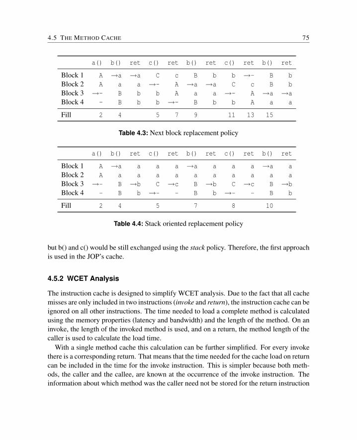
4.5 THE METHOD CACHE 75
a() b() ret c() ret b() ret c() ret b() ret
Block 1 A →a →a C c B b b →- B bBlock 2 A a a →- A →a →a C c B bBlock 3 →- B b b A a a →- A →a →aBlock 4 - B b b →- B b b A a a
Fill 2 4 5 7 9 11 13 15
Table 4.3: Next block replacement policy
a() b() ret c() ret b() ret c() ret b() ret
Block 1 A →a a a a →a a a a →a aBlock 2 A a a a a a a a a a aBlock 3 →- B →b C →c B →b C →c B →bBlock 4 - B b →- - B b →- - B b
Fill 2 4 5 7 8 10
Table 4.4: Stack oriented replacement policy
but b() and c() would be still exchanged using the stack policy. Therefore, the first approachis used in the JOP’s cache.
4.5.2 WCET Analysis
The instruction cache is designed to simplify WCET analysis. Due to the fact that all cachemisses are only included in two instructions (invoke and return), the instruction cache can beignored on all other instructions. The time needed to load a complete method is calculatedusing the memory properties (latency and bandwidth) and the length of the method. On aninvoke, the length of the invoked method is used, and on a return, the method length of thecaller is used to calculate the load time.
With a single method cache this calculation can be further simplified. For every invokethere is a corresponding return. That means that the time needed for the cache load on returncan be included in the time for the invoke instruction. This is simpler because both meth-ods, the caller and the callee, are known at the occurrence of the invoke instruction. Theinformation about which method was the caller need not be stored for the return instruction
76 4 HARDWARE ARCHITECTURE
to be analyzed.
With more than one method in the cache, a cache hit detection has to be performed aspart of the WCET analysis. If there are only two blocks, this is trivial, as (i) a hit on invokeis only possible if the method is the same as the last invoked (e.g. a single method in a loop)and (ii) a hit on return is only possible when the method is a leaf in the call tree. In the lattercase, it is always a hit.
When the cache contains more blocks (i.e. more than two methods can be cached), a partof the call tree has to be taken into account for hit detection. The method cache furthercomplicates the analysis, as the method length also determines the cache content. However,this analysis is still simpler than a cache modeling of a direct-mapped instruction cache, ascache block replacement depends on the call tree instead of instruction addresses.
WCET analysis of cache hits for the method cache is most beneficial for methods invokedin a loop, where the methods are classified as first miss. The basic idea of the method cacheanalysis is as follows: Within a loop it is statically analyzed if all methods invoked and theinvoking method, which contains the loop, fit together in the method cache. If this is thecase, all methods will at most miss once. The concrete implementation of the the analysisalgorithm is described in [66].
Except for leaf methods, the cache load can be triggered by an invoke instruction ofby a return instruction. On an invoke some of the miss penalty is hidden by concurrentmicrocode execution. Therefore, we have to assume the higher cost of loading methodsinto the cache on a return instruction for non-leaf methods. Leaf nodes can naturally onlymiss on an invoke.
In traditional caches, data access and instruction cache fill requests can compete for themain memory bus. For example, a load or store at the end of the processor pipeline com-petes with an instruction fetch that results in a cache miss. One of the two instructions isstalled for additional cycles by the other instruction. With a data cache, this situation canbe even worse. The worst-case scenario for the memory stall time for an instruction fetchor a data load is two miss penalties when both cache reads are a miss. This unpredictablebehavior leads to very pessimistic WCET bounds.
A method cache, with cache fills only on invoke and return, does not interfere with dataaccess to the main memory. Data in the main memory is accessed with getfield and put-field, instructions that never overlap with invoke and return. This property removes anotheruncertainty found in traditional cache designs.
4.5 THE METHOD CACHE 77
4.5.3 Caches Compared
In this section, we compare two different cache architectures in a quantitative way. Al-though our primary concern is predictability, performance remains important. We willtherefore first present the results from a conventional direct-mapped instruction cache.These measurements provide a baseline for the evaluation of the described cache archi-tecture.
Cache performance varies with different application domains. As the system is intendedfor real-time applications, the benchmark for these tests should reflect this fact. However,there are no standard benchmarks available for embedded real-time systems. A real-timeapplication was therefore adapted to create this benchmark. The application is from onenode of a distributed motor control system [117] (see also Section 11.4.1). A simulation ofthe environment (sensors and actors) and the communication system (commands from themaster station) forms part of the benchmark for simulating the real-world workload.
The data for all measurements was captured using a simulation of JOP and running theapplication for 500,000 clock cycles. During this time, the major loop of the application wasexecuted several hundred times, effectively rendering any misses during the initializationcode irrelevant to the measurements. As the embedded application is quite small (1366LOC), small instruction caches have been simulated.
WCET analysis based comparison of the method cache and of standard instruction cachesis currently under development. Therefore, we perform only average case measurements fora comparison between a time-predictable cache organization and a standard cache organiza-tion. With a simulation of JOP, we measure the cache misses and miss penalties for differentconfigurations of the method cache and a direct-mapped cache. The miss penalty and theresulting effect on the execution time depend on the main memory system. Therefore, wesimulate three different memory technologies: static RAM (SRAM), synchronous DRAM(SDRAM), and double data rate (DDR) SDRAM. For the SRAM, a latency of 1 clock cy-cle and an access time of 2 clock cycles per 32-bit word are assumed. For the SDRAM,a latency of 5 cycles (3 cycles for the row address and 2 cycles for the CAS latency) isassumed. The SDRAM delivers one word (4 bytes) per cycle. The DDR SDRAM has ashorter latency of 4.5 cycles and transfers data on both the rising and falling edge of theclock signal.
The resulting miss cycles are scaled to the bandwidth consumed by the instruction fetchunit. The result is the number of cache fill cycles per fetched instruction byte. In otherwords: the average main memory access time in cycles per instruction byte. A value of 0.1means that for every 10 fetched instruction bytes, one clock cycle is spent to fill the cache.
Table 4.5 shows the result for different configurations of a direct-mapped cache. Which
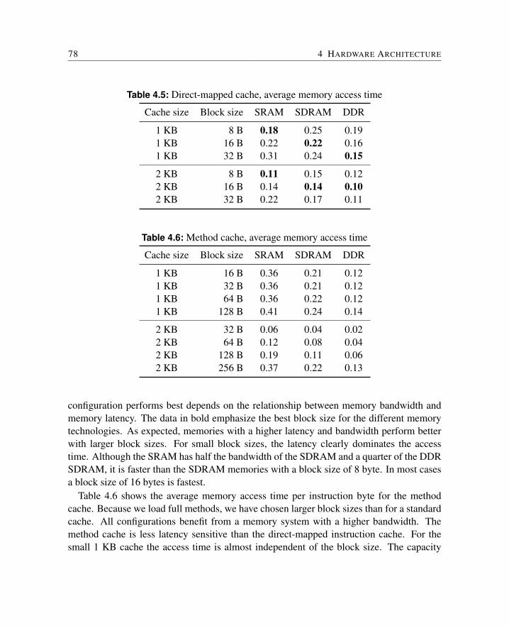
78 4 HARDWARE ARCHITECTURE
Table 4.5: Direct-mapped cache, average memory access time
Cache size Block size SRAM SDRAM DDR
1 KB 8 B 0.18 0.25 0.191 KB 16 B 0.22 0.22 0.161 KB 32 B 0.31 0.24 0.15
2 KB 8 B 0.11 0.15 0.122 KB 16 B 0.14 0.14 0.102 KB 32 B 0.22 0.17 0.11
Table 4.6: Method cache, average memory access time
Cache size Block size SRAM SDRAM DDR
1 KB 16 B 0.36 0.21 0.121 KB 32 B 0.36 0.21 0.121 KB 64 B 0.36 0.22 0.121 KB 128 B 0.41 0.24 0.14
2 KB 32 B 0.06 0.04 0.022 KB 64 B 0.12 0.08 0.042 KB 128 B 0.19 0.11 0.062 KB 256 B 0.37 0.22 0.13
configuration performs best depends on the relationship between memory bandwidth andmemory latency. The data in bold emphasize the best block size for the different memorytechnologies. As expected, memories with a higher latency and bandwidth perform betterwith larger block sizes. For small block sizes, the latency clearly dominates the accesstime. Although the SRAM has half the bandwidth of the SDRAM and a quarter of the DDRSDRAM, it is faster than the SDRAM memories with a block size of 8 byte. In most casesa block size of 16 bytes is fastest.
Table 4.6 shows the average memory access time per instruction byte for the methodcache. Because we load full methods, we have chosen larger block sizes than for a standardcache. All configurations benefit from a memory system with a higher bandwidth. Themethod cache is less latency sensitive than the direct-mapped instruction cache. For thesmall 1 KB cache the access time is almost independent of the block size. The capacity
4.5 THE METHOD CACHE 79
misses dominate. From the 2 KB configuration we see that smaller block sizes result in lesscache misses. However, smaller block sizes result in more hardware for the hit detectionsince the method cache is in effect fully associatively. Therefore, we need a balance betweenthe number of blocks and the performance.
The cache conflict is high for the small configuration with 1 KB cache. The direct-mapped cache, backed up with a low-latency main memory, performs better than the methodcache. When high-latency memories are used, the method cache performs better than thedirect mapped cache. This is expected as the long latency for a transfer is amortized whenmore data (the whole method) is filled in one request.
A small block size of 32 Bytes is needed in the 2 KB method cache to outperform thedirect mapped cache with the low-latency main memory as represented by the SRAM. Forhigher latency memories (SDRAM and DDR), a method cache with a block size of 128bytes outperforms the direct mapped instruction cache.
The comparison does not show if the method cache is more easily predictable than othercache solutions. It shows that caching full methods performs similarly to standard cachingtechniques.
4.5.4 Summary
From the properties of the Java language – usually small methods and relative branches– we derived the novel idea of a method cache, i.e. a cache organization in which wholemethods are loaded into the cache on method invocation and the return from a method. Thiscache organization is time-predictable, as all cache misses are lumped together in these twoinstructions. Using only one block for a single method introduces considerable overheadsin comparison with a conventional cache, but is very simple to analyze. We extended thiscache to hold more methods, with several smaller blocks per method.
Comparing these organizations quantitatively with a benchmark derived from a real-timeapplication, we have seen that the method cache performs similarly to (and in some configu-rations even better than) a direct-mapped cache. Only filling the cache on method invocationand return simplifies WCET analysis and removes another source of uncertainty, as there isno competition for the main memory access between instruction cache and data cache.

5 Runtime System
A Java processor alone is not a complete JVM. This chapter describes the definition of areal-time profile for Java and the description of the JVM internal data structures to representclasses and objects.
5.1 A Real-Time Profile for Embedded Java
As standard Java is under-specified for real-time systems and the RTSJ does not fit forsmall embedded systems a new and simpler real-time profile is defined in this section andimplemented on JOP. The guidelines of the specification are:
• High-integrity profile
• Easy syntax
• Easy to implement
• Low runtime overhead
• No syntactic extension of Java
• Minimum change of Java semantics
• Support for time measurement if a WCET analysis tool is not available
• Known overheads (documentation of runtime behavior and memory requirements ofevery JVM operation and all methods have to be provided)
The real-time profile under discussion is inspired by the restricted versions of the RTSJdescribed in [111] and [77]. It is intended for high-integrity real-time applications and as atest case to evaluate the architecture of JOP as a Java processor for real-time systems.
The proposed definition is not compatible with the RTSJ. Since the application domainfor the RTSJ is different from high-integrity systems, it makes sense for it not to be compat-ible with the RTSJ. Restrictions can be enforced by defining new classes (e.g. setting thread
82 5 RUNTIME SYSTEM
priority in the constructor of a real-time thread alone, enforcing minimum interarrival timesfor sporadic events).
To verify that this specification is expressive enough for high-integrity real-time appli-cations, Ravenscar-Java (RJ) [77], with the additional necessary RTSJ classes, has beenimplemented on top of it. However, RJ inherits some of the complexity of the RTSJ. There-fore, the implementation of RJ has a larger memory and runtime overhead than this simplespecification.
When the specification for Safety-Critical Java (JSR 302)1 [64] will be finalized the pro-file will be adapted for this specification.
5.1.1 Application Structure
The application is divided in two different phases: initialization and mission. All non time-critical initialization, global object allocations, thread creation and startup are performedin the initialization phase. All classes need to be loaded and initialized in this phase. Themission phase starts after invocation of startMission(). The number of threads is fixed and theassigned priorities remain unchanged. The following restrictions apply to the application:
• Initialization and mission phase
• Fixed number of threads
• Threads are created at initialization phase
• All shared objects are allocated at initialization
5.1.2 Threads
Concurrency is expressed with two types of schedulable objects:
Periodic activities are represented by threads that execute in an infinite loop invoking wait-ForNextPeriod() to get rescheduled in predefined time intervals.
Asynchronous sporadic activities are represented by event handlers. Each event handleris in fact a thread, which is released by an hardware interrupt or a software generatedevent (invocation of fire()). Minimum interarrival time has to be specified on creationof the event handler.
1http://jcp.org/en/jsr/detail?id=302
5.1 A REAL-TIME PROFILE FOR EMBEDDED JAVA 83
The classes that implement the schedulable objects are:
RtThread represents a periodic task. As usual task work is coded in run(), which getsinvoked on missionStart(). A scoped memory object can be attached to an RtThread atcreation.
SwEvent represents a software-generated event. It is triggered by fire() and needs to over-ride handle().
Listing 5.1 shows the definition of the basic classes. Listing 5.2 shows the principlecoding of a worker thread. An example for creation of two real-time threads and an eventhandler can be seen in Listing 5.3.
5.1.3 Scheduling
The scheduler is a preemptive, priority-based scheduler with unlimited priority levels anda unique priority value for each schedulable object. No real-time threads or events arescheduled during the initialization phase.
The design decision to use unique priority levels, instead of FIFO within priorities, isbased on following facts: Two common ways to assign priorities are rate monotonic and, ina more general form, deadline monotonic assignment. When two tasks are given the samepriority, we can choose one of them and assign a higher priority to that task and the task setwill still be schedulable. This results in a strictly monotonic priority order and we do notneed to deal with FIFO order. This eliminates queues for each priority level and results in asingle, priority ordered task list with unlimited priority levels.
Synchronized blocks are executed with priority ceiling emulation protocol. In the currentimplementation top priority is assumed for all objects. This avoids priority inversions onobjects that are not accessible from the application (e.g. objects inside a library).
5.1.4 Memory
The profile does not support a garbage collector.2 All memory should be allocated at theinitialization phase. Without a garbage collector, the heap implicitly becomes immortalmemory (as defined by the RTSJ). Scoped memory is currently in a prototyping stage, butwill be supported in the future.
2This restriction can be relaxed when the real-time GC for JOP is used (see Chapter 7).
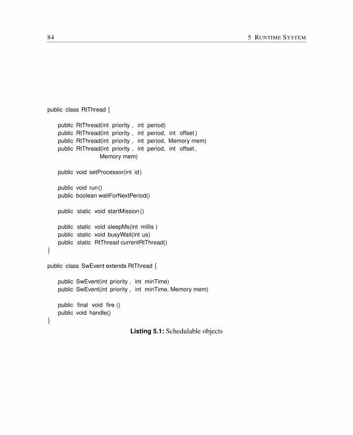
84 5 RUNTIME SYSTEM
public class RtThread {
public RtThread(int priority , int period)public RtThread(int priority , int period, int offset )public RtThread(int priority , int period, Memory mem)public RtThread(int priority , int period, int offset ,
Memory mem)
public void setProcessor(int id )
public void run()public boolean waitForNextPeriod()
public static void startMission ()
public static void sleepMs(int millis )public static void busyWait(int us)public static RtThread currentRtThread()
}
public class SwEvent extends RtThread {
public SwEvent(int priority , int minTime)public SwEvent(int priority , int minTime, Memory mem)
public final void fire ()public void handle()
}Listing 5.1: Schedulable objects
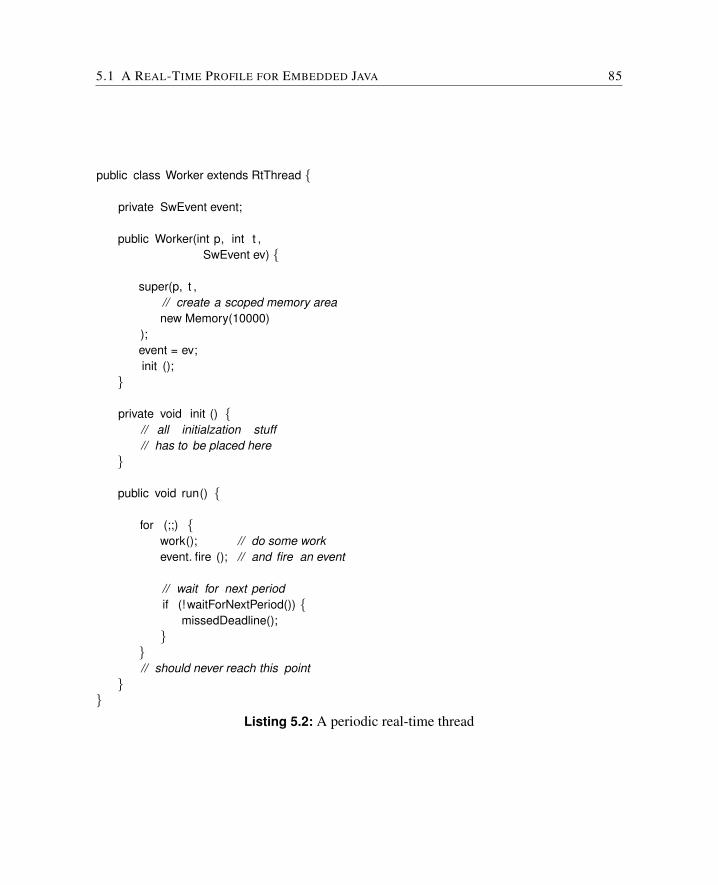
5.1 A REAL-TIME PROFILE FOR EMBEDDED JAVA 85
public class Worker extends RtThread {
private SwEvent event;
public Worker(int p, int t ,SwEvent ev) {
super(p, t ,// create a scoped memory areanew Memory(10000)
);event = ev;init ();
}
private void init () {// all initialzation stuff// has to be placed here
}
public void run() {
for (;;) {work(); // do some workevent. fire (); // and fire an event
// wait for next periodif (! waitForNextPeriod()) {
missedDeadline();}
}// should never reach this point
}}
Listing 5.2: A periodic real-time thread
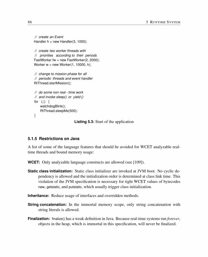
86 5 RUNTIME SYSTEM
// create an EventHandler h = new Handler(3, 1000);
// create two worker threads with// priorities according to their periodsFastWorker fw = new FastWorker(2, 2000);Worker w = new Worker(1, 10000, h);
// change to mission phase for all// periodic threads and event handlerRtThread.startMission();
// do some non real−time work// and invoke sleep() or yield ()for (;;) {
watchdogBlink();RtThread.sleepMs(500);
}Listing 5.3: Start of the application
5.1.5 Restrictions on Java
A list of some of the language features that should be avoided for WCET analyzable real-time threads and bound memory usage:
WCET: Only analyzable language constructs are allowed (see [109]).
Static class initialization: Static class initializer are invoked at JVM boot. No cyclic de-pendency is allowed and the initialization order is determined at class link time. Thisviolation of the JVM specification is necessary for tight WCET values of bytecodesnew, getstatic, and putstatic, which usually trigger class initialization.
Inheritance: Reduce usage of interfaces and overridden methods.
String concatenation: In the immortal memory scope, only string concatenation withstring literals is allowed.
Finalization: finalize() has a weak definition in Java. Because real-time systems run forever,objects in the heap, which is immortal in this specification, will never be finalized.
5.1 A REAL-TIME PROFILE FOR EMBEDDED JAVA 87
Dynamic Class Loading: Due to the implementation and WCET analysis complexity dy-namic class loading is avoided.
5.1.6 Interaction of RtThread, the Scheduler, and the JVM
Figure 5.1 shows an interaction example of the scheduler, the application, and the JVM.The interaction diagram shows the message sequences between two application tasks, thescheduler, the JVM and the hardware. The hardware represents interrupt and timer logic.Task 2 is a periodic task with a higher priority than Task 1.
The first event is a timer event to unblock Task 2 for a new period. The generated timerevent results in a call of the scheduler. The scheduler performs its scheduling decision andissues a context switch to Task 2. With every context switch the timer is reprogrammedto generate an interrupt at the next time triggered event for a higher priority task. Task 2performs the periodic work and ceases execution by invocation of waitForNextPeriod(). Thescheduler is called and requests an interrupt from the hardware resulting in the same callsequence as with a timer. The software generated interrupt imposes negligible overheadand results in a single entry point for the scheduler. Task 1 is the only ready task in thisexample and is resumed by the scheduler.
5.1.7 Implementation Results
The initial idea was to implement scheduling and dispatching in microcode. However, manyJava bytecodes have a one to one mapping to a microcode instruction, resulting in a singlecycle execution. The performance gain of an algorithm coded in microcode is thereforenegligible. As a result, almost all of the scheduling is implemented in Java. Only a smallpart of the dispatcher, a memory copy, is implemented in microcode and exposed with aspecial bytecode.
Experimental results of basic scheduling benchmarks, such as periodic thread jitter, con-text switch time for threads and asynchronous events, can be found in [119].
To implement system functions, such as scheduling, in Java, access to JVM and processorinternal data structures have to be available. However, Java does not allow memory accessor access to hardware devices. In JOP, this access is provided by additional bytecodes.In the Java environment, these bytecodes are represented as static native methods. Thecompiled invoke instruction for these methods (invokestatic) is replaced by these additionalbytecodes in the class file. This solution provides a very efficient way to incorporate low-level functions into a pure Java system. The translation can be performed during classloading to avoid non-standard class files.
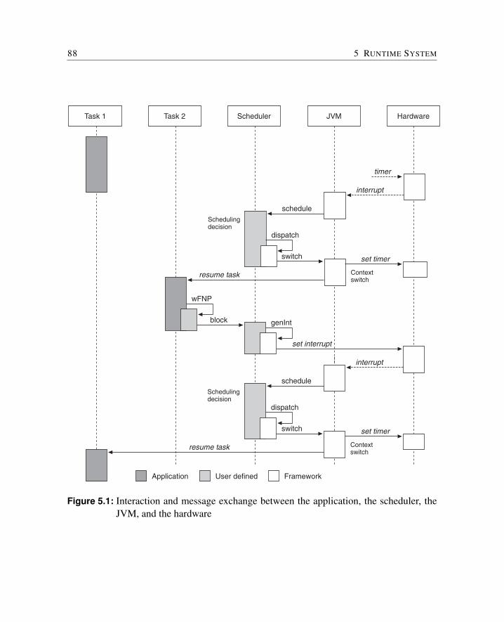
88 5 RUNTIME SYSTEM
Task 1 SchedulerTask 2 JVM Hardware
block genInt
set interrupt
interrupt
schedule
dispatch
switch
resume task
Schedulingdecision
Contextswitch
wFNP
interrupt
schedule
dispatch
Schedulingdecision
Contextswitch
timer
User defined FrameworkApplication
resume task
set timer
set timer
switch
Figure 5.1: Interaction and message exchange between the application, the scheduler, theJVM, and the hardware
5.2 A PROFILE FOR SAFETY CRITICAL JAVA 89
A pure Java system, without an underlying RTOS, is an unusual system with some inter-esting new properties. Java is a safer execution environment than C (e.g. no pointers) andthe boundary between kernel and user space can become quite loose. Scheduling, usuallypart of the operating system or the JVM, is implemented in Java and executed in the samecontext as the application.
This property provides an easy path to a framework for user-defined scheduling. In [118]a framework for a user defined scheduler for JOP is presented. The events that result in thescheduling decision are listed. Hooks for these events allow the implementation of a userdefined scheduler.
5.1.8 Summary
This section consider a simple profile for real-time Java and the implementation of real-timescheduling on a Java processor. The novelty of the described approach is in implementingfunctions usually associated with an RTOS in Java. That means that real-time Java is notbased on an RTOS, and therefore not restricted to the functionality provided by the RTOS.With JOP, a self-contained real-time system in pure Java becomes possible. The imple-mentation of the specification is successfully used as the basis for a commercial real-timeapplication in the railway industry.
5.2 A Profile for Safety Critical Java
The proposed profile is an refinement of the profile described in Section 5.1. Further de-velopment of applications on JOP shall be based on this profile and the current applications(e.g. OBB bg and Lift) should be migrated to this profile.
5.2.1 Introduction
Safety-critical Java (SCJ) builds upon a broad research base on using Java (and Ada) forhard real-time systems, sometimes also called high integrity systems. The Ravenscar profiledefines a subset of Ada to support development of safety-critical systems [39]. Based onthe concepts of Ravenscar Ada a restriction of the RTSJ was first proposed in [111]. Theserestrictions are similar to SCJ level 1 without the mission concept. The idea was furtherextended in [77] and named the Ravenscar Java profile (RJ). RJ is an extended subset ofRTSJ that removes features considered unsafe for high integrity systems. Another profilefor safety-critical systems was proposed within the EU project HIJA [1].
90 5 RUNTIME SYSTEM
PERC Pico from Aonix [6] defines a Java environment for hard real-time systems. PERCPico defines its own class hierarchy for real-time Java classes which are based on the RTSJlibraries, but are not a strict subset thereof. PERC Pico introduces stack-allocated scopes,an elaborate annotation system, and an integrated static analysis system to verify scopesafety and analyze memory and CPU time resource requirements for hard real-time softwarecomponents. Some of the annotations used to describe the libraries of the SCJ are derivedindirectly from the annotation system used in PERC Pico.
Another definition of a profile for safety-critical Java was published in [137]. In contrastto RJ the authors of that profile argue for new classes instead of reusing RTSJ based classesto avoid inheriting unsafe RTSJ features and to simplify the class hierarchy. A proposalfor mission modes within the former profile [126] permits recycling CPU time budgets fordifferent phases of the application. Compared to the mission concept of SCJ that proposalallows periodic threads to vote against the shutdown of a mission. The concept of missionmemory is not part of that proposal.
In this chapter we focus on the safety-critical Java (SCJ) specification, a new standardfor safety critical applications developed by the JSR 302 expert group [64]. We should notethat the JSR 302 has not been finalized, thus we present the version from [126]. Whenthe JSR 302 stabilizes it will be implemented for JOP and will be the future version of thereal-time profile.
5.2.2 SCJ Level 1
Level 1 of the SCJ requires that all threads be defined during an initial initialization phase.This phase is run only once at virtual machine startup. The second phase, called the missionphase, begins only when all threads have been started. This phase runs until virtual ma-chine shutdown. Level 1 supports only two kinds of schedulable objects: periodic threadsand sporadic events. The latter can be generated by either hardware or software. This re-strictions keeps the schedulability analysis simple. In SCJ priority ceiling emulation is thedefault monitor control policy. The default ceiling is top priority.
The Java wait and notify primitives are not allowed in SCJ level 0 and 1. This furthersimplifies analysis. The consequence is that a thread context switch can only occur if ahigher priority thread is released or if the current running thread yields (in the case of SCJby returning from the run() method).
In the RTSJ, periodic tasks are expressed by unbounded loops with, at some point, a callto the waitForNextPeriod() (or wFNP() for short) method of class RealtimeThread. This has theeffect of yielding control to the scheduler which will only wake the thread when its nextperiod starts or shortly thereafter. In SCJ, as a simplification, periodic logic is encapsulated
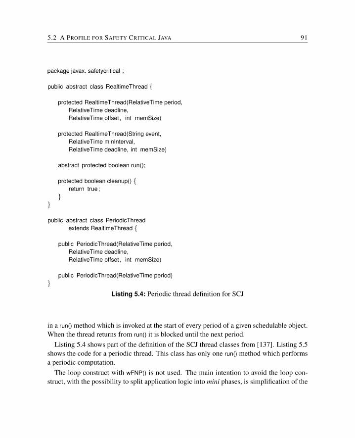
5.2 A PROFILE FOR SAFETY CRITICAL JAVA 91
package javax. safetycritical ;
public abstract class RealtimeThread {
protected RealtimeThread(RelativeTime period,RelativeTime deadline,RelativeTime offset, int memSize)
protected RealtimeThread(String event,RelativeTime minInterval,RelativeTime deadline, int memSize)
abstract protected boolean run();
protected boolean cleanup() {return true;
}}
public abstract class PeriodicThreadextends RealtimeThread {
public PeriodicThread(RelativeTime period,RelativeTime deadline,RelativeTime offset, int memSize)
public PeriodicThread(RelativeTime period)}
Listing 5.4: Periodic thread definition for SCJ
in a run() method which is invoked at the start of every period of a given schedulable object.When the thread returns from run() it is blocked until the next period.
Listing 5.4 shows part of the definition of the SCJ thread classes from [137]. Listing 5.5shows the code for a periodic thread. This class has only one run() method which performsa periodic computation.
The loop construct with wFNP() is not used. The main intention to avoid the loop con-struct, with the possibility to split application logic into mini phases, is simplification of the
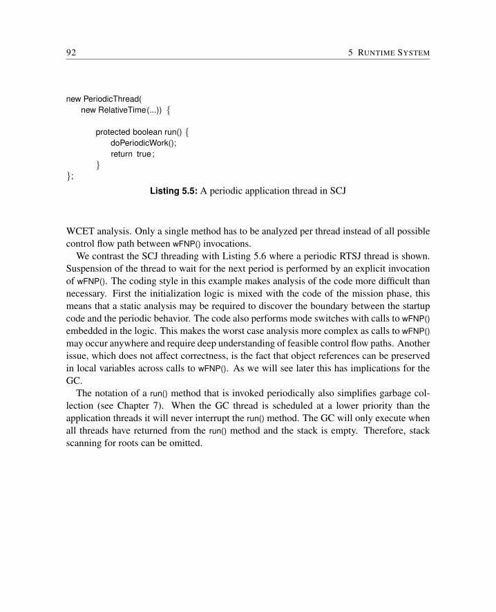
92 5 RUNTIME SYSTEM
new PeriodicThread(new RelativeTime(...)) {
protected boolean run() {doPeriodicWork();return true;
}};
Listing 5.5: A periodic application thread in SCJ
WCET analysis. Only a single method has to be analyzed per thread instead of all possiblecontrol flow path between wFNP() invocations.
We contrast the SCJ threading with Listing 5.6 where a periodic RTSJ thread is shown.Suspension of the thread to wait for the next period is performed by an explicit invocationof wFNP(). The coding style in this example makes analysis of the code more difficult thannecessary. First the initialization logic is mixed with the code of the mission phase, thismeans that a static analysis may be required to discover the boundary between the startupcode and the periodic behavior. The code also performs mode switches with calls to wFNP()embedded in the logic. This makes the worst case analysis more complex as calls to wFNP()may occur anywhere and require deep understanding of feasible control flow paths. Anotherissue, which does not affect correctness, is the fact that object references can be preservedin local variables across calls to wFNP(). As we will see later this has implications for theGC.
The notation of a run() method that is invoked periodically also simplifies garbage col-lection (see Chapter 7). When the GC thread is scheduled at a lower priority than theapplication threads it will never interrupt the run() method. The GC will only execute whenall threads have returned from the run() method and the stack is empty. Therefore, stackscanning for roots can be omitted.
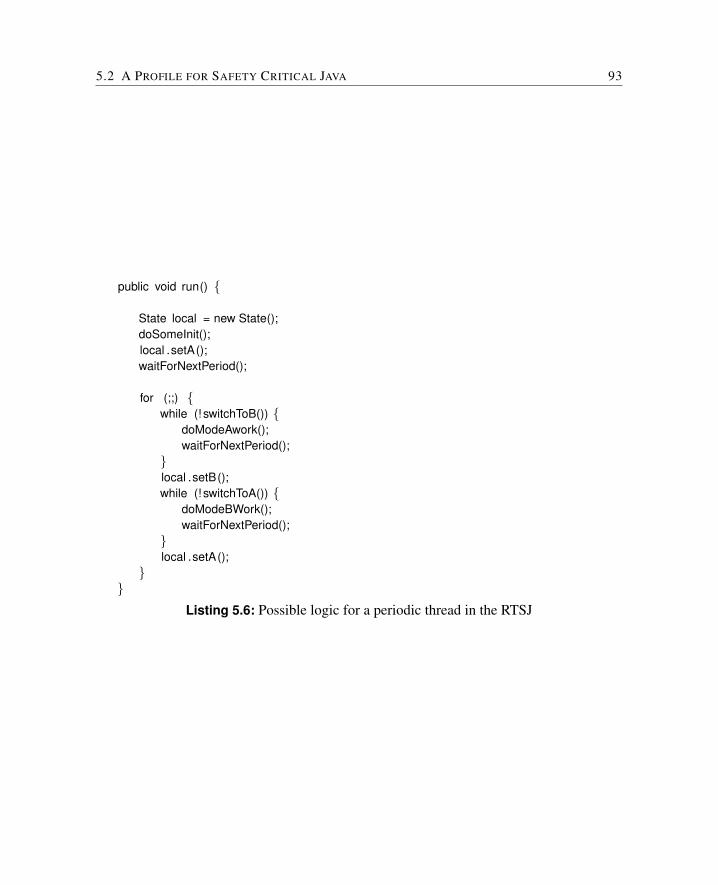
5.2 A PROFILE FOR SAFETY CRITICAL JAVA 93
public void run() {
State local = new State();doSomeInit();local .setA();waitForNextPeriod();
for (;;) {while (! switchToB()) {
doModeAwork();waitForNextPeriod();
}local .setB();while (! switchToA()) {
doModeBWork();waitForNextPeriod();
}local .setA();
}}
Listing 5.6: Possible logic for a periodic thread in the RTSJ
94 5 RUNTIME SYSTEM
5.3 JVM Architecture
This section presents the details of the implementation of the JVM on JOP. The represen-tation of objects and the stack frame is chosen to support JOP as a processor for real-timesystems. However, since the data structures are realized through microcode they can beeasily changed for a system with different needs.
5.3.1 Runtime Data Structures
Memory is addressed as 32-bit data, which means that memory pointers are incremented forevery four bytes. No single byte or 16-bit access is necessary. The abstract type referenceis a pointer (via a handle indirection) to memory that represents the object or an array. Thereference is pushed on the stack before an instruction can operate on it. A null reference isrepresented by the value 0.
Stack Frame
On invocation of a method, the invoker’s context is saved in a newly allocated frame on thestack. It is restored when the method returns. The saved context consists of the followingregisters:
SP: Immediately before invocation, the stack pointer points to the last argument for thecalled function. This value is reduced by the argument count (i.e. the arguments areconsumed) and saved in the new stack frame.
PC: The pointer to the next bytecode instruction after the invoke instruction.
VP: The pointer to the memory area on the stack that contains the locals.
CP: The pointer to the constant pool of the class from the invoking method.
MP: The pointer to the method structure of the invoking method.
SP, PC and VP are registers in JOP while CP and MP are local variables of the JVM.Figure 5.2 provides an example of the stack before and after invoking a method. In thisexample, the called method has two arguments and contains two local variables. If themethod is a virtual one, the first argument is the reference to the object (the this-pointer).The arguments implicitly become locals in the called method and are accessed in the sameway as local variables. The start of the stack frame (Frame in the figure) needs not to be
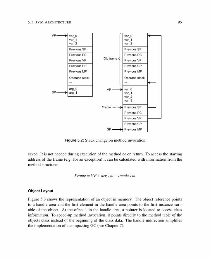
5.3 JVM ARCHITECTURE 95
var_0var_1var_2
Previous SP
Previous MP
Previous CP
Previous VP
Previous PC
Operand stack...
arg_0arg_1
var_0var_1var_2
Previous SP
Previous MP
Previous CP
Previous VP
Previous PC
Operand stack...
var_0var_1var_2var_3
Previous SP
Previous MP
Previous CP
Previous VP
Previous PC
VP
SPVP
Frame
SP
Old frame
Figure 5.2: Stack change on method invocation
saved. It is not needed during execution of the method or on return. To access the startingaddress of the frame (e.g. for an exception) it can be calculated with information from themethod structure:
Frame = V P+arg cnt + locals cnt
Object Layout
Figure 5.3 shows the representation of an object in memory. The object reference pointsto a handle area and the first element in the handle area points to the first instance vari-able of the object. At the offset 1 in the handle area, a pointer is located to access classinformation. To speed-up method invocation, it points directly to the method table of theobjects class instead of the beginning of the class data. The handle indirection simplifiesthe implementation of a compacting GC (see Chapter 7).
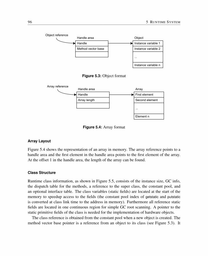
96 5 RUNTIME SYSTEM
Instance variable 1
Method vector base
Handle
Instance variable 2
...
Instance variable n
Object referenceHandle area Object
Figure 5.3: Object format
First element
Array length
Handle
Second element
...
Element n
Array referenceHandle area Array
Figure 5.4: Array format
Array Layout
Figure 5.4 shows the representation of an array in memory. The array reference points to ahandle area and the first element in the handle area points to the first element of the array.At the offset 1 in the handle area, the length of the array can be found.
Class Structure
Runtime class information, as shown in Figure 5.5, consists of the instance size, GC info,the dispatch table for the methods, a reference to the super class, the constant pool, andan optional interface table. The class variables (static fields) are located at the start of thememory to speedup access to the fields (the constant pool index of getstatic and putstaticis converted at class link time to the address in memory). Furthermore all reference staticfields are located in one continuous region for simple GC root scanning. A pointer to thestatic primitive fields of the class is needed for the implementation of hardware objects.
The class reference is obtained from the constant pool when a new object is created. Themethod vector base pointer is a reference from an object to its class (see Figure 5.3). It
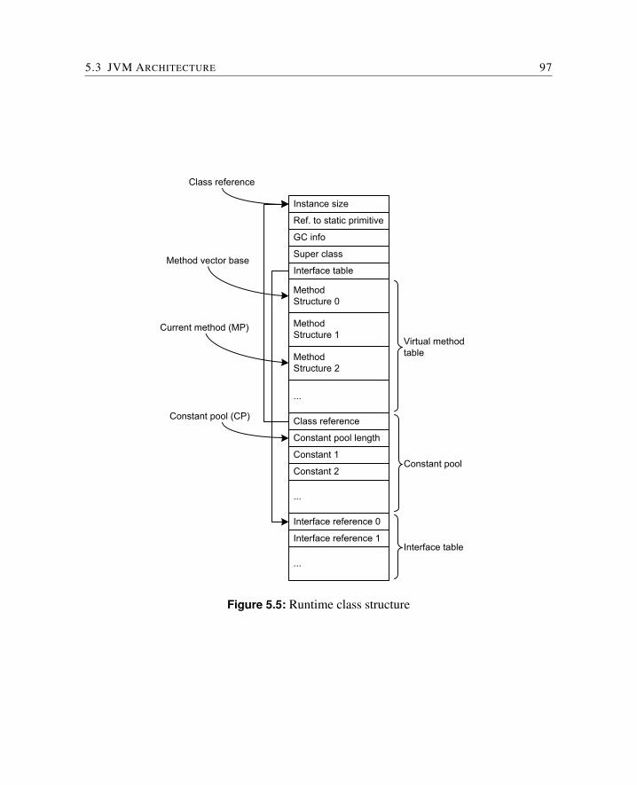
5.3 JVM ARCHITECTURE 97
Constant pool length
Instance size
Ref. to static primitive
GC info
Super class
Interface table
MethodStructure 0
Class reference
Interface reference 0
MethodStructure 1
MethodStructure 2
...
Constant 1
Constant 2
...
Interface reference 1
...
Virtual method table
Constant pool
Interface table
Class reference
Method vector base
Current method (MP)
Constant pool (CP)
Figure 5.5: Runtime class structure
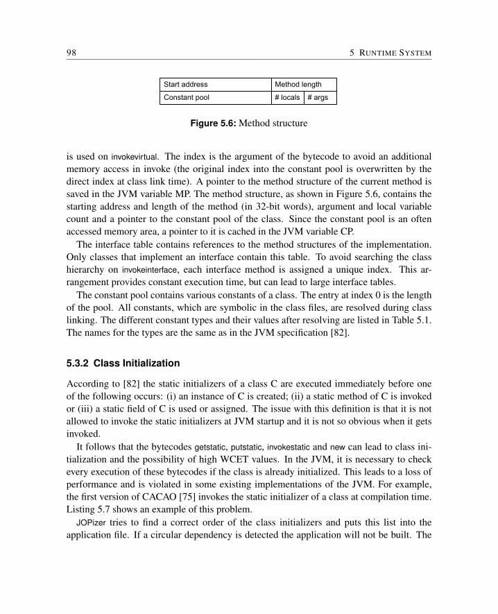
98 5 RUNTIME SYSTEM
Method length
# locals # args
Start address
Constant pool
Figure 5.6: Method structure
is used on invokevirtual. The index is the argument of the bytecode to avoid an additionalmemory access in invoke (the original index into the constant pool is overwritten by thedirect index at class link time). A pointer to the method structure of the current method issaved in the JVM variable MP. The method structure, as shown in Figure 5.6, contains thestarting address and length of the method (in 32-bit words), argument and local variablecount and a pointer to the constant pool of the class. Since the constant pool is an oftenaccessed memory area, a pointer to it is cached in the JVM variable CP.
The interface table contains references to the method structures of the implementation.Only classes that implement an interface contain this table. To avoid searching the classhierarchy on invokeinterface, each interface method is assigned a unique index. This ar-rangement provides constant execution time, but can lead to large interface tables.
The constant pool contains various constants of a class. The entry at index 0 is the lengthof the pool. All constants, which are symbolic in the class files, are resolved during classlinking. The different constant types and their values after resolving are listed in Table 5.1.The names for the types are the same as in the JVM specification [82].
5.3.2 Class Initialization
According to [82] the static initializers of a class C are executed immediately before oneof the following occurs: (i) an instance of C is created; (ii) a static method of C is invokedor (iii) a static field of C is used or assigned. The issue with this definition is that it is notallowed to invoke the static initializers at JVM startup and it is not so obvious when it getsinvoked.
It follows that the bytecodes getstatic, putstatic, invokestatic and new can lead to class ini-tialization and the possibility of high WCET values. In the JVM, it is necessary to checkevery execution of these bytecodes if the class is already initialized. This leads to a loss ofperformance and is violated in some existing implementations of the JVM. For example,the first version of CACAO [75] invokes the static initializer of a class at compilation time.Listing 5.7 shows an example of this problem.
JOPizer tries to find a correct order of the class initializers and puts this list into theapplication file. If a circular dependency is detected the application will not be built. The
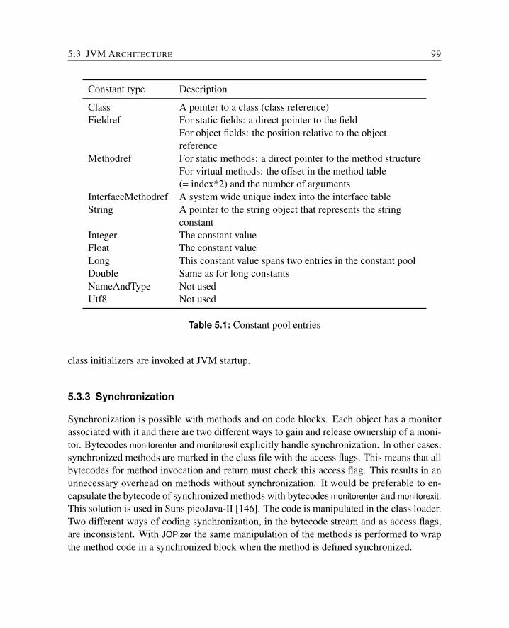
5.3 JVM ARCHITECTURE 99
Constant type Description
Class A pointer to a class (class reference)Fieldref For static fields: a direct pointer to the field
For object fields: the position relative to the objectreference
Methodref For static methods: a direct pointer to the method structureFor virtual methods: the offset in the method table(= index*2) and the number of arguments
InterfaceMethodref A system wide unique index into the interface tableString A pointer to the string object that represents the string
constantInteger The constant valueFloat The constant valueLong This constant value spans two entries in the constant poolDouble Same as for long constantsNameAndType Not usedUtf8 Not used
Table 5.1: Constant pool entries
class initializers are invoked at JVM startup.
5.3.3 Synchronization
Synchronization is possible with methods and on code blocks. Each object has a monitorassociated with it and there are two different ways to gain and release ownership of a moni-tor. Bytecodes monitorenter and monitorexit explicitly handle synchronization. In other cases,synchronized methods are marked in the class file with the access flags. This means that allbytecodes for method invocation and return must check this access flag. This results in anunnecessary overhead on methods without synchronization. It would be preferable to en-capsulate the bytecode of synchronized methods with bytecodes monitorenter and monitorexit.This solution is used in Suns picoJava-II [146]. The code is manipulated in the class loader.Two different ways of coding synchronization, in the bytecode stream and as access flags,are inconsistent. With JOPizer the same manipulation of the methods is performed to wrapthe method code in a synchronized block when the method is defined synchronized.
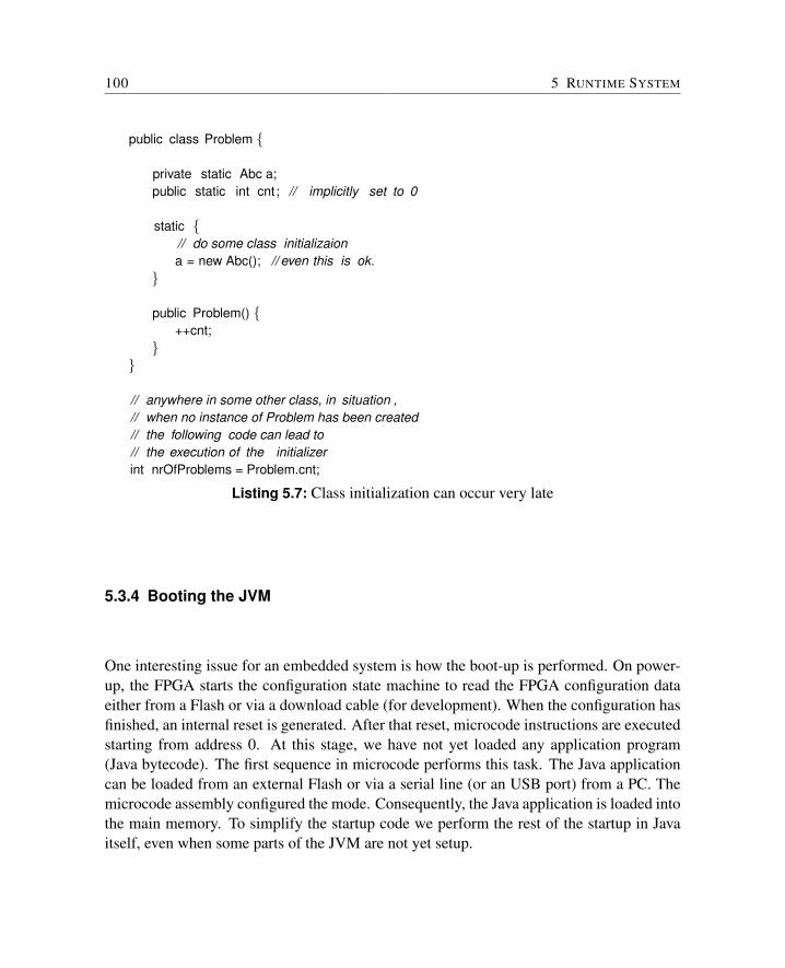
100 5 RUNTIME SYSTEM
public class Problem {
private static Abc a;public static int cnt; // implicitly set to 0
static {// do some class initializaiona = new Abc(); // even this is ok.
}
public Problem() {++cnt;
}}
// anywhere in some other class, in situation ,// when no instance of Problem has been created// the following code can lead to// the execution of the initializerint nrOfProblems = Problem.cnt;
Listing 5.7: Class initialization can occur very late
5.3.4 Booting the JVM
One interesting issue for an embedded system is how the boot-up is performed. On power-up, the FPGA starts the configuration state machine to read the FPGA configuration dataeither from a Flash or via a download cable (for development). When the configuration hasfinished, an internal reset is generated. After that reset, microcode instructions are executedstarting from address 0. At this stage, we have not yet loaded any application program(Java bytecode). The first sequence in microcode performs this task. The Java applicationcan be loaded from an external Flash or via a serial line (or an USB port) from a PC. Themicrocode assembly configured the mode. Consequently, the Java application is loaded intothe main memory. To simplify the startup code we perform the rest of the startup in Javaitself, even when some parts of the JVM are not yet setup.
5.3 JVM ARCHITECTURE 101
In the next step, a minimal stack frame is generated and the special method Startup.boot()is invoked. From now on JOP runs in Java mode. The method boot() performs the followingsteps:
1. Send a greeting message to stdout
2. Detect the size of the main memory
3. Initialize the data structures for the garbage collector
4. Initialize java.lang.System
5. Print out JOP’s version number, detected clock speed, and memory size
6. Invoke the static class initializers in a predefined order
7. Invoke the main method of the application class

6 Worst-Case Execution Time
Worst-case execution time (WCET) estimates of tasks are essential for designing and veri-fying real-time systems. WCET estimates can be obtained either by measurement or staticanalysis. The problem with using measurements is that the execution times of tasks tendto be sensitive to their inputs. As a rule, measurement does not guarantee safe WCET es-timates. Instead, static analysis is necessary for hard real-time systems. Static analysis isusually divided into a number of different phases:
Path analysis generates the control flow graph (a directed graph of basic blocks) of theprogram and annotates (manual or automatic) loops with bounds.
Low-level analysis determines the execution time of basic blocks obtained by the pathanalysis. A model of the processor and the pipeline provides the execution time forthe instruction sequence.
Global low-level analysis determines the influence of hardware features such as caches onprogram execution time. This analysis can use information from the path analysis toprovide less pessimistic values.
WCET Calculation The final WCET is calculated by transforming the control flow graphwith the timing information of basic blocks1 with the program annotations for loopsto an integer linear programming (ILP) problem. This problem is solved by an ILPsolver. This approach is also called implicit path enumeration (IPET).
For the low-level analysis, a good timing model of the processor is needed. The mainproblem for the low-level analysis is the execution time dependency of instructions in mod-ern processors that are not designed for real-time systems. JOP is designed to be an easytarget for WCET analysis. The WCET of each bytecode can be predicted in terms of thenumber of cycles it requires. There are no timing dependencies between bytecodes.
WCET analysis has to be done at two levels: at the microcode level and at the bytecodelevel. The microcode WCET analysis is performed only once for a processor configuration
1A basic block is a sequence of instructions without any jumps or jump targets within this sequence.
104 6 WORST-CASE EXECUTION TIME
and described in the next section. The result from this microcode analysis is the timingmodel of the processor. The timing model is the input for WCET analysis at the bytecodelevel (i.e. the Java application) as explained in Section 6.2.
The first WCET analysis tool that targets JOP has been developed by Rasmus Pedersen[134]. Benedikt Huber implemented a new version of the analyzer with support of byte-codes implemented in Java and a better method cache approximation has [67]. The newtool also contains a module to extract the low-level bytecode timing from the microcodeassembler program (jvm.asm) automatically.
6.1 Microcode WCET Analysis
Each bytecode is implemented by microcode. We can obtain the WCET of a single byte-code by performing WCET analysis at the microcode level. To prove that there are notime dependencies between bytecodes, we have to show that no processor states are sharedbetween different bytecodes.
6.1.1 Microcode Path Analysis
To obtain the WCET values for the individual bytecodes we perform the path analysis atthe microcode level. First, we have to ensure that a number of restrictions (from [109]) ofthe code are fulfilled:
• Programs must not contain unbounded recursion. This property is satisfied by thefact that there exists no call instruction in microcode.
• Function pointers and computed gotos complicate the path analysis and should there-fore be avoided. Only simple conditional branches are available at the microcodelevel.
• The upper bound of each loop has to be known. This is the only point that has to beverified by inspection of the microcode.
To detect loops in the microcode we have to find all backward branches (e.g. with a negativebranch offset).2 The branch offsets can be found in a VHDL file (offtbl.vhd) that is generatedduring microcode assembly. In the current implementation of the JVM there are ten differ-ent negative offsets. However, not each offset represents a loop. Most of these branches
2The loop branch can be a forward branch. However, the basic blocks of the loop contain at least one backwardbranch. Therefore we can identify all loops by searching for backward branches only.

6.1 MICROCODE WCET ANALYSIS 105
are used to share common code. Three branches are found in the initialization code of theJVM. They are not part of a bytecode implementation and can be ignored. The only loopthat is found in a regular bytecode is in the implementation of imul to perform a fixed delay.The iteration count for this loop is constant.
A few bytecodes are implemented in Java3 and can be analyzed in the same way as appli-cation code. The bytecodes idiv and irem contain a constant loop. The bytecode lookupswitch4
performs a linear search through a table of branch offsets. The WCET depends on the tablesize that can be found as part of the instruction.
As the microcode sequences are very short, the calculation of the control flow graph foreach bytecode is done manually.
6.1.2 Microcode Low-level Analysis
To calculate the execution time of basic blocks in the microcode, we need to establish thetiming of microcode instructions on JOP. All microcode instructions except wait execute ina single cycle, reducing the low-level analysis to a case of merely counting the instructions.
The wait instruction is used to stall the processor and wait for the memory subsystem tofinish a memory transaction. The execution time of the wait instruction depends on the mem-ory system and, if the memory system is predictable, has a known WCET. A main memoryconsisting of SRAM chips can provide this predictability and this solution is therefore ad-vised. The predictable handling of DMA, which is used for the instruction cache fill, isexplained in Section 4.5. The wait instruction is the only way to stall the processor. Hard-ware events, such as interrupts (see Section 4.3.5), do not stall the processor.
Microcode is stored in on-chip memory with single cycle access. Each microcode in-struction is a single word long and there is no need for either caching or prefetching at thisstage. We can therefore omit the low-level analysis. No pipeline analysis [42], with itspossible unbounded timing effects, is necessary.
6.1.3 Bytecode Independency
We have seen that all microcode instructions except wait take one cycle to execute and aretherefore independent of other instructions. This property directly translates to indepen-dency of bytecode instructions.
3The implementation can be found in the class com.jopdesign.sys.JVM.4lookupswitch is one way of implementing the Java switch statement. The other bytecode, tableswitch, uses
an index in the table of branch offsets and has therefore a constant execution time.
106 6 WORST-CASE EXECUTION TIME
The wait microcode instruction provides a convenient way to hide memory access time.A memory read or write can be triggered in microcode and the processor can continuewith microcode instructions. When the data from a memory read is needed, the processorexplicitly waits, with the wait instruction, until it becomes available.
For a memory store, this wait could be deferred until the memory system is used next(similar to a write buffer). It is possible to initiate the store in a bytecode such as putfield andcontinue with the execution of the next bytecode, even when the store has not been com-pleted. In this case, we introduce a dependency over bytecode boundaries, as the state of thememory system is shared. To avoid these dependencies that are difficult to analyze, eachbytecode that accesses memory waits (preferably at the end of the microcode sequence) forthe completion of the memory request.
Furthermore, if we would not wait at the end of the store operation we would have toinsert an additional wait at the start of every read operation. Since read operations are morefrequent than write operations (15% vs. 2.5%, see [123]), the performance gain from thehidden memory store is lost.
6.1.4 WCET of Bytecodes
The control flow of the individual bytecodes together with the basic block length (thatdirectly corresponds with the execution time) and the time for memory access result in theWCET (and BCET) values of the bytecodes. These values can be found in Appendix D.
Basic Bytecodes
Most bytecode instructions that do not access memory have a constant execution time.They are executed by either one microcode instruction or a short sequence of microcodeinstructions. The execution time in clock cycles equals the number of microinstructionsexecuted. As the stack is on-chip, it can be accessed in a single cycle. We do not need toincorporate the main memory timing into the instruction timing. Most simple bytecodesexecute in a single cycle. Table 6.1 shows example instructions, their timing, and theirmeaning. Access to object, array, and class fields depend on the timing of the main memory.
Object Oriented Bytecodes
Object oriented instructions, array access, and invoke instructions access the main memory.Therefore, we have to model the memory access time. We assume a simple SRAM with aconstant access time. Access time that exceeds a single cycle includes additional wait states
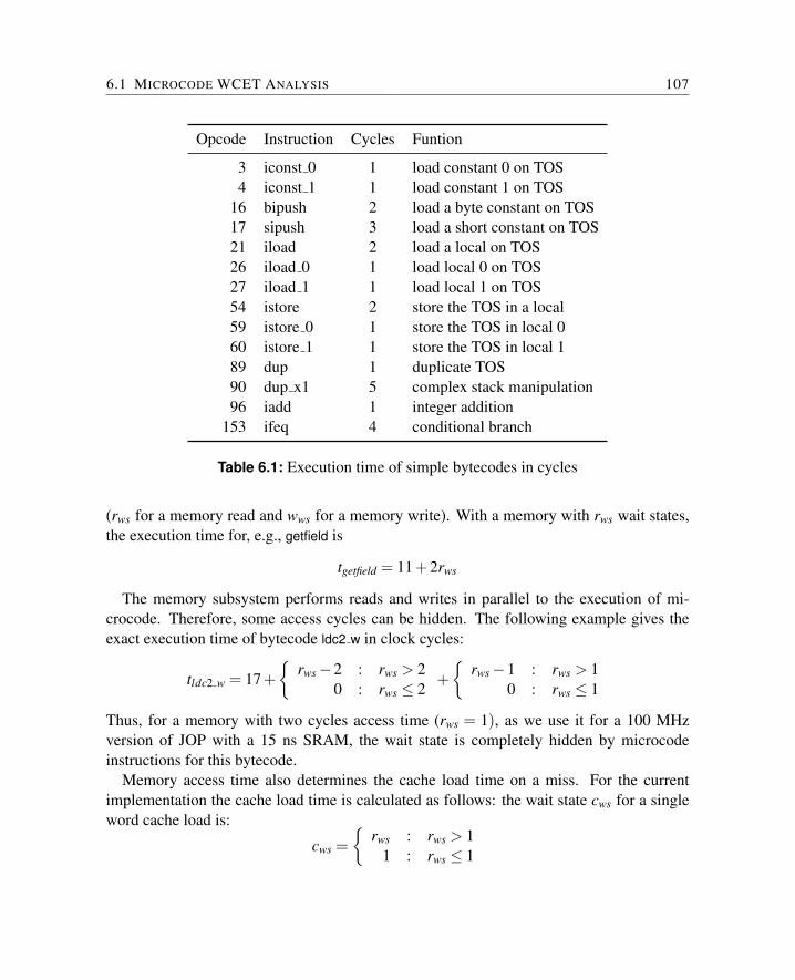
6.1 MICROCODE WCET ANALYSIS 107
Opcode Instruction Cycles Funtion
3 iconst 0 1 load constant 0 on TOS4 iconst 1 1 load constant 1 on TOS
16 bipush 2 load a byte constant on TOS17 sipush 3 load a short constant on TOS21 iload 2 load a local on TOS26 iload 0 1 load local 0 on TOS27 iload 1 1 load local 1 on TOS54 istore 2 store the TOS in a local59 istore 0 1 store the TOS in local 060 istore 1 1 store the TOS in local 189 dup 1 duplicate TOS90 dup x1 5 complex stack manipulation96 iadd 1 integer addition
153 ifeq 4 conditional branch
Table 6.1: Execution time of simple bytecodes in cycles
(rws for a memory read and wws for a memory write). With a memory with rws wait states,the execution time for, e.g., getfield is
tgetfield = 11+2rws
The memory subsystem performs reads and writes in parallel to the execution of mi-crocode. Therefore, some access cycles can be hidden. The following example gives theexact execution time of bytecode ldc2 w in clock cycles:
tldc2 w = 17+{
rws−2 : rws > 20 : rws ≤ 2
+{
rws−1 : rws > 10 : rws ≤ 1
Thus, for a memory with two cycles access time (rws = 1), as we use it for a 100 MHzversion of JOP with a 15 ns SRAM, the wait state is completely hidden by microcodeinstructions for this bytecode.
Memory access time also determines the cache load time on a miss. For the currentimplementation the cache load time is calculated as follows: the wait state cws for a singleword cache load is:
cws ={
rws : rws > 11 : rws ≤ 1
108 6 WORST-CASE EXECUTION TIME
On a method invoke or return, the respective method has to be loaded into the cache on acache miss. The load time l is:
l ={
6+(n+1)(1+ cws) : cache miss4 : cache hit
where n is the size of the method in number of 32-bit words. For short methods, the loadtime of the method on a cache miss, or part of it, is hidden by microcode execution. As anexample, the exact execution time for the bytecode invokestatic is:
t = 74+ rws +{
rws−3 : rws > 30 : rws ≤ 3
+{
rws−2 : rws > 24 : rws ≤ 2
+{
l−37 : l > 370 : l ≤ 37
For invokestatic a cache load time l of up to 37 cycles is completely hidden. For theexample SRAM timing the cache load of methods up to 36 bytes long is hidden. The WCETanalysis tool, as described in the next section, knows the length of the invoked method andcan therefore calculate the time for the invoke instruction cycle accurate.
Bytecodes in Java
Bytecodes can be implemented in Java on JOP. In this case, a static method from a JVMinternal class gets invoked when such a bytecode is executed. For WCET analysis thisbytecode is substituted by an invoke instruction to this method. The influence on the cache(the bytecode execution results in a method load) can be analyzed in the same way as forordinary static methods.
Native Methods
Most of the JVM internal functionality in JOP, such as input, output, and thread scheduling,is implemented in Java. However, Java and the JVM do not allow direct access to memory,peripheral devices or processor registers. For this low-level access to system resources,we need native methods. For a Java processor, the native language is still Java bytecode.We solve this issue by substituting the native method invocation by a special bytecodeinstruction on class loading. Those special bytecodes are implemented in JOP microcodein the same way as regular bytecodes (see Section 4.2. The execution time of the nativemethods (or in other words special bytecodes) is given in the same way as the executiontime for standard bytecodes.
6.2 WCET ANALYSIS OF THE JAVA APPLICATION 109
6.2 WCET Analysis of the Java Application
In hard real-time systems, the estimation of the worst-case execution time (WCET) is essen-tial. WCET analysis is in general an undecidable problem. Program restrictions, as givenin [109], make this problem decidable:
1. Programs must not contain any recursion
2. Absence of function pointers
3. The upper bound of each loop has to be known
Recursive algorithms have to be transformed to iterative ones. For our WCET analyzer,the loop bounds are detected by data-flow analysis or have to be annotated in the programsource. However, we want to relax the second restriction regarding function pointers. Func-tion pointers are similar to inherited or overridden methods: they are dispatched at runtime.For an object-oriented language this mechanism is fundamental. In contrast to functionpointers, e.g., in C, we can statically analyze which methods can be invoked when thewhole program is known. Therefore, we allow dynamic dispatching of methods in Java inour analysis.
We replace the function pointer restriction by the following restriction: Dynamic classloading is not allowed. As the full application has to be available for WCET analysis,dynamic class loading cannot be supported. For embedded real-time systems this is not asevere restriction.
6.2.1 High-Level WCET Analysis
The high-level WCET analysis, presented in this section, is based on standard technologies[110, 79]. From the class files that make up the application, the relevant information isextracted. The CFG of the basic blocks is extracted from the bytecodes. Annotations forthe loop counts are either provided by the data-flow analysis or are extracted from commentsin the source. Furthermore, the class hierarchy is examined to find all possible targets for amethod invoke and the data-flow analysis tightens the set of possible receivers.
Java bytecode generation has to follow stringent rules [82] in order to pass the class fileverification of the JVM. Those restrictions lead to an analysis friendly code; e.g. the stacksize is known at each instruction. The control flow instructions are well defined. Branchesare relative and the destination is within the same method. In the normal program, there is
110 6 WORST-CASE EXECUTION TIME
no instruction that loads a branch destination in a local variable or onto the stack.5 Detectionof basic blocks in Java bytecode and construction of the CFG is thus straight forward.
In Java class files there is more information available than in compiled C/C++ executa-bles. All links are symbolic and it is possible to reconstruct the class hierarchy from theclass files. Therefore, we can statically determine all possible targets for a virtual methodinvoke.
WCET analysis at the bytecode level has several advantages when the execution time ofthe individual bytecodes are known. When compiled with debug information referencesto the source are stored in the class file. With this information it is possible to extractannotations in the Java source code. We use this feature to annotated loop bounds withincomments in the Java source. This form of annotation is simple and less intrusive than usinga predefined dummy class as suggested in [23].
6.2.2 WCET Annotations
Simple loop bounds are detected by the data-flow analysis [104]. For cases where thebounds are not detectable, we additionally support annotations in the source. The annota-tions are written as comments (see Listing 6.1). It would be more convenient to use standardJava annotations introduced with Java 1.5, as they are checked at compile time. However,at the moment Java annotations are not allowed at code block level. A proposal to removethis restriction is currently under review (JSR 308). When compiling Java, the source lineinformation is included in the class file. Therefore, when a loop is detected in the CFG,the relevant source line for the loop header is looked up in the source and the annotation isextracted from the comment.
Annotations given as source comments are simple and less intrusive than using a prede-fined dummy class [23]. Two variants of the loop bounding annotation are supported: onewith an exact bound6 (=) and one that places an upper bound on the iterations (<=). Theextension to more elaborate annotations, as suggested in [109] and [23], can provide eventighter WCET bounds.
5The exception are bytecodes jsr and ret that use the stack and a local variable for the return address of amethod local subroutine. This construct can be used to implement the finally clauses of the Java program-ming language. However, this problematic subroutine can be easily inlined [12]. Furthermore, Sun’s Javacompilers version 1.4.2 and later compile finally blocks without subroutines.
6The exact bound has been used to find best-case values for some test settings.
6.2 WCET ANALYSIS OF THE JAVA APPLICATION 111
6.2.3 ILP Formulation
The calculation of the WCET is transformed to an ILP problem [110]. In the CFG, eachvertex represents a basic block Bi with execution time ci. With the basic block executionfrequency ei the WCET is:
WCET = maxN
∑i=1
ciei
The sum is the objective function for the ILP problem. The maximum value of this expres-sion results in the WCET of the program.
Furthermore, each edge is also assigned an execution frequency f . These executionfrequencies represent the control flow through the WCET path. Two primary constraintsform the ILP problem: (i) For each vertex, the sum of f j for the incoming edges has to beequal to the sum of the fk of the outgoing edges; (ii) The frequency of the edges connectingthe loop body with the loop header, is less than or equal to the frequency of the edgesentering the loop multiplied by the loop bound.
From the CFG, which represents the program structure, we can extract the flow con-straints. With the execution frequency f of the edges and the two sets Ii for the incomingedges to basic block Bi and Oi for the outgoing edges, the execution frequency ei of Bi is:
ei = ∑j∈Ii
f j = ∑k∈Oi
fk
The frequencies f are the integer variables calculated by solving the ILP problem. Further-more, we add two special vertices to the graph: The start node S and the termination nodeT . The start node S has only one outgoing edge that points to the first basic block of theprogram. The execution frequency fs of this edge is set to 1. The termination node T hasonly incoming edges with the sum of the frequencies also set to 1; all return statements ofa method are connected to the node T . This means that the program is executed once andcan only terminate once through T .
Loop bounds are additional constraints for the ILP problem. A special vertex, the loopheader, is connected by following edges:
1. Incoming edges that enter the loop with frequency fh
2. One outgoing edge entering the loop body with frequency fl
3. Incoming edges that close the loop
4. One loop exit edge
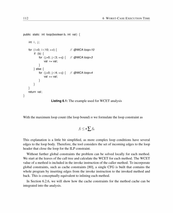
112 6 WORST-CASE EXECUTION TIME
public static int loop(boolean b, int val ) {
int i , j ;
for ( i=0; i<10; ++i) { // @WCA loop=10if (b) {
for ( j=0; j<3; ++j) { // @WCA loop=3val ∗= val ;
}} else {
for ( j=0; j<4; ++j) { // @WCA loop=4val += val;
}}
}return val ;
}Listing 6.1: The example used for WCET analysis
With the maximum loop count (the loop bound) n we formulate the loop constraint as
fl ≤ n∑ fh
This explanation is a little bit simplified, as more complex loop conditions have severaledges to the loop body. Therefore, the tool considers the set of incoming edges to the loopheader that close the loop for the ILP constraint.
Without further global constraints the problem can be solved locally for each method.We start at the leaves of the call tree and calculate the WCET for each method. The WCETvalue of a method is included in the invoke instruction of the caller method. To incorporateglobal constraints, such as cache constraints [80], a single CFG is built that contains thewhole program by inserting edges from the invoke instruction to the invoked method andback. This is conceptually equivalent to inlining each method.
In Section 6.2.6, we will show how the cache constraints for the method cache can beintegrated into the analysis.
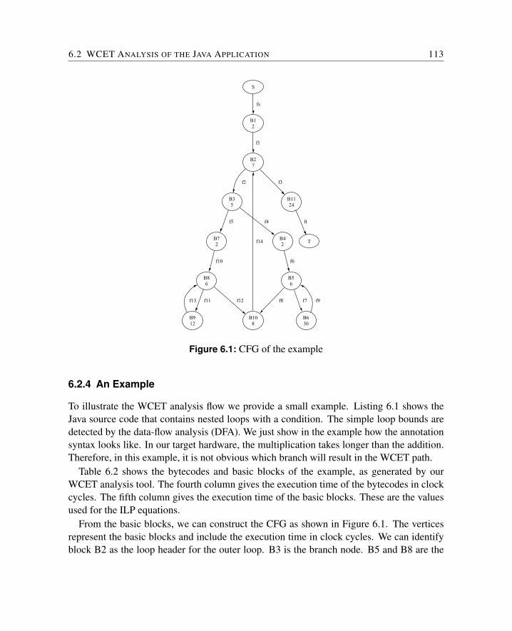
6.2 WCET ANALYSIS OF THE JAVA APPLICATION 113
S
B12
fs
B27
f1
B35
f2
B1124
f3
B42
f4
B72
f5
T
ft
B56
f6
B86
f10
B630
f7
B108
f8 f9
f14
f12
B912
f11f13
Figure 6.1: CFG of the example
6.2.4 An Example
To illustrate the WCET analysis flow we provide a small example. Listing 6.1 shows theJava source code that contains nested loops with a condition. The simple loop bounds aredetected by the data-flow analysis (DFA). We just show in the example how the annotationsyntax looks like. In our target hardware, the multiplication takes longer than the addition.Therefore, in this example, it is not obvious which branch will result in the WCET path.
Table 6.2 shows the bytecodes and basic blocks of the example, as generated by ourWCET analysis tool. The fourth column gives the execution time of the bytecodes in clockcycles. The fifth column gives the execution time of the basic blocks. These are the valuesused for the ILP equations.
From the basic blocks, we can construct the CFG as shown in Figure 6.1. The verticesrepresent the basic blocks and include the execution time in clock cycles. We can identifyblock B2 as the loop header for the outer loop. B3 is the branch node. B5 and B8 are the
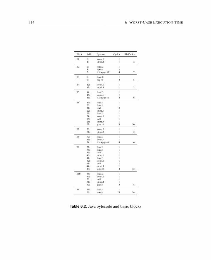
114 6 WORST-CASE EXECUTION TIME
Block Addr. Bytecode Cycles BB Cycles
B1 0: iconst 0 11: istore 2 1 2
B2 2: iload 2 13: bipush 25: if icmpge 55 4 7
B3 8: iload 0 19: ifeq 30 4 5
B4 12: iconst 0 113: istore 3 1 2
B5 14: iload 3 115: iconst 3 116: if icmpge 48 4 6
B6 19: iload 1 120: iload 1 121: imul 1922: istore 1 123: iload 3 124: iconst 1 125: iadd 126: istore 3 127: goto 14 4 30
B7 30: iconst 0 131: istore 3 1 2
B8 32: iload 3 133: iconst 4 134: if icmpge 48 4 6
B9 37: iload 1 138: iload 1 139: iadd 140: istore 1 141: iload 3 142: iconst 1 143: iadd 144: istore 3 145: goto 32 4 12
B10 48: iload 2 149: iconst 1 150: iadd 151: istore 2 152: goto 2 4 8
B11 55: iload 1 156: ireturn 23 24
Table 6.2: Java bytecode and basic blocks
6.2 WCET ANALYSIS OF THE JAVA APPLICATION 115
loop headers for the inner loops.From the CFG, we can extract the flow constraints by the following fact: The execution
frequency of a basic block is equal to the execution frequency of all incoming edges andequal to the execution frequency of all outgoing edges. E.g., for block B2 the executionfrequency e2 is:
e2 = f1 + f14 = f2 + f3
The loop constraints are formulated by constraining the frequency of the loop’s backedges. The loop bounds are automatically transferred from the DFA module or extractedfrom the source annotations. For the outer loop in the example this is:
f14 = 10 f1
In Listing 6.2, the resulting equations for the integer linear programming problem, asgenerated by our tool, are listed. We use the open-source ILP solver lp solve.7
The ILP solver lp solve gives a result of 1393 cycles. We run this example on the Javaprocessor for verification. As the execution time depends only on a single boolean variable,b (see Listing 6.1), it is trivial to measure the actual WCET. We measure the execution timewith a cycle counter for the execution time of the outer loop, i.e., from the start of blockB1 until the exit of the loop at block B2. The last block, B11, which contains the returnstatement, is not part of the measurement. The measured result is 1369 cycles. When weadd the 24 cycles for the block B11 to our measured WCET, we get 1393 cycles. Thismeasured result is exactly the same as the analytical result!
6.2.5 Dynamic Method Dispatch
Dynamic runtime-dispatching of inherited or overridden instance methods is a key featureof object-oriented programming. Therefore, we allow dynamic methods as a controlledform of function pointers. The full class hierarchy can be extracted from the class files ofthe application. From the class hierarchy, we can extract all possible receiver methods foran invocation. When all possible receivers are included as alternatives, the resulting WCETbound can be very pessimistic. Therefore, this set can be tightened by a flow-sensitivereceiver analysis [104].
We include all possible receivers as alternatives in the ILP constraints. It has to be notedthat, without further analysis or annotations, this can lead to pessimistic WCET estimates.
7http://lpsolve.sourceforge.net/5.5/
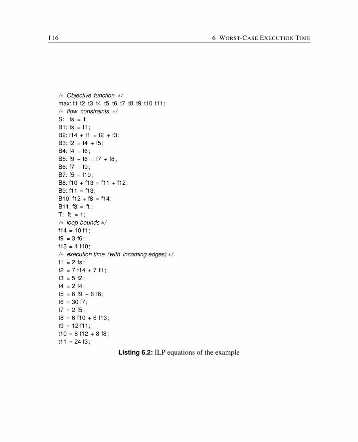
116 6 WORST-CASE EXECUTION TIME
/∗ Objective function ∗/max: t1 t2 t3 t4 t5 t6 t7 t8 t9 t10 t11;/∗ flow constraints ∗/S: fs = 1;B1: fs = f1 ;B2: f14 + f1 = f2 + f3 ;B3: f2 = f4 + f5 ;B4: f4 = f6 ;B5: f9 + f6 = f7 + f8 ;B6: f7 = f9 ;B7: f5 = f10;B8: f10 + f13 = f11 + f12;B9: f11 = f13;B10: f12 + f8 = f14;B11: f3 = ft ;T: ft = 1;/∗ loop bounds ∗/f14 = 10 f1;f9 = 3 f6 ;f13 = 4 f10;/∗ execution time (with incoming edges) ∗/t1 = 2 fs ;t2 = 7 f14 + 7 f1 ;t3 = 5 f2 ;t4 = 2 f4 ;t5 = 6 f9 + 6 f6 ;t6 = 30 f7;t7 = 2 f5 ;t8 = 6 f10 + 6 f13;t9 = 12 f11;t10 = 8 f12 + 8 f8 ;t11 = 24 f3;
Listing 6.2: ILP equations of the example
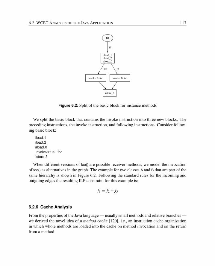
6.2 WCET ANALYSIS OF THE JAVA APPLICATION 117
B1
iload_1iload_2aload_0
f1
invoke A.foo
f2
invoke B.foo
f3
istore_3
Figure 6.2: Split of the basic block for instance methods
We split the basic block that contains the invoke instruction into three new blocks: Thepreceding instructions, the invoke instruction, and following instructions. Consider follow-ing basic block:
iload 1iload 2aload 0invokevirtual fooistore 3
When different versions of foo() are possible receiver methods, we model the invocationof foo() as alternatives in the graph. The example for two classes A and B that are part of thesame hierarchy is shown in Figure 6.2. Following the standard rules for the incoming andoutgoing edges the resulting ILP constraint for this example is:
f1 = f2 + f3
6.2.6 Cache Analysis
From the properties of the Java language — usually small methods and relative branches —we derived the novel idea of a method cache [120], i.e., an instruction cache organizationin which whole methods are loaded into the cache on method invocation and on the returnfrom a method.
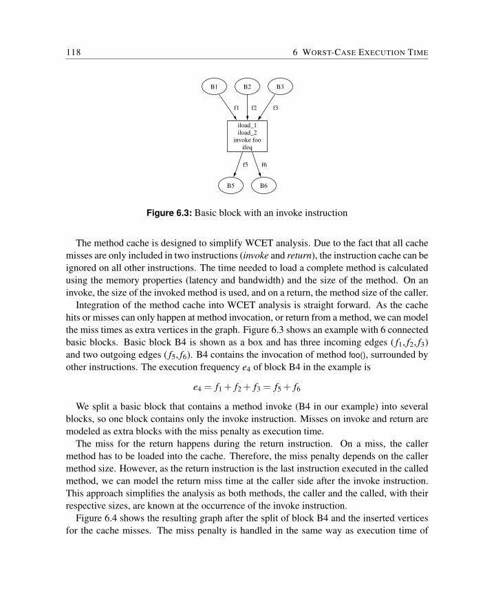
118 6 WORST-CASE EXECUTION TIME
B1
iload_1iload_2
invoke fooifeq
f1
B5
f5
B6
f6
B2
f2
B3
f3
Figure 6.3: Basic block with an invoke instruction
The method cache is designed to simplify WCET analysis. Due to the fact that all cachemisses are only included in two instructions (invoke and return), the instruction cache can beignored on all other instructions. The time needed to load a complete method is calculatedusing the memory properties (latency and bandwidth) and the size of the method. On aninvoke, the size of the invoked method is used, and on a return, the method size of the caller.
Integration of the method cache into WCET analysis is straight forward. As the cachehits or misses can only happen at method invocation, or return from a method, we can modelthe miss times as extra vertices in the graph. Figure 6.3 shows an example with 6 connectedbasic blocks. Basic block B4 is shown as a box and has three incoming edges ( f1, f2, f3)and two outgoing edges ( f5, f6). B4 contains the invocation of method foo(), surrounded byother instructions. The execution frequency e4 of block B4 in the example is
e4 = f1 + f2 + f3 = f5 + f6
We split a basic block that contains a method invoke (B4 in our example) into severalblocks, so one block contains only the invoke instruction. Misses on invoke and return aremodeled as extra blocks with the miss penalty as execution time.
The miss for the return happens during the return instruction. On a miss, the callermethod has to be loaded into the cache. Therefore, the miss penalty depends on the callermethod size. However, as the return instruction is the last instruction executed in the calledmethod, we can model the return miss time at the caller side after the invoke instruction.This approach simplifies the analysis as both methods, the caller and the called, with theirrespective sizes, are known at the occurrence of the invoke instruction.
Figure 6.4 shows the resulting graph after the split of block B4 and the inserted verticesfor the cache misses. The miss penalty is handled in the same way as execution time of
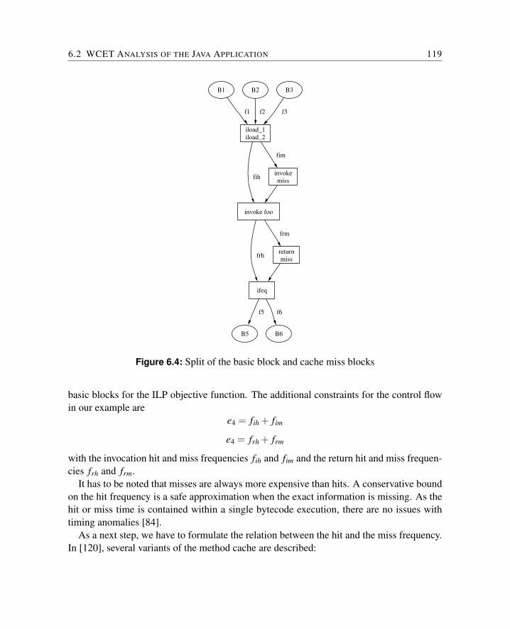
6.2 WCET ANALYSIS OF THE JAVA APPLICATION 119
B1
iload_1iload_2
f1
invoke foo
fihinvokemiss
fim
B2
f2
B3
f3
ifeq
frhreturnmiss
frm
B5
f5
B6
f6
Figure 6.4: Split of the basic block and cache miss blocks
basic blocks for the ILP objective function. The additional constraints for the control flowin our example are
e4 = fih + fim
e4 = frh + frm
with the invocation hit and miss frequencies fih and fim and the return hit and miss frequen-cies frh and frm.
It has to be noted that misses are always more expensive than hits. A conservative boundon the hit frequency is a safe approximation when the exact information is missing. As thehit or miss time is contained within a single bytecode execution, there are no issues withtiming anomalies [84].
As a next step, we have to formulate the relation between the hit and the miss frequency.In [120], several variants of the method cache are described:
120 6 WORST-CASE EXECUTION TIME
1. A single block that can only cache a single method
2. Several blocks that each can cache a single method
3. A variable block cache where a method can span several blocks
The first two variants are simple to integrate into WCET analysis, but lead to high WCETbounds. In the following, the analysis of the third variant is described, details on analysisof the first two variants can be found in [134].
The variable block cache divides the cache in several blocks similar to cache lines ina conventional cache. However, a single method has to be loaded in a continuous regionof the cache. The effective replacement policy of the variable block cache is FIFO. FIFOcaches need a long access history for standard classification techniques [112]. Due to theFIFO replacement, one can construct examples where a method in a loop can be classifiedas single miss, but that miss does not need to happen at the first iteration or it can happenon a return from an invoked method.
WCET analysis of cache hits for the method cache is most beneficial for methods invokedin a loop, where the methods are classified as first miss. The basic idea of the method cacheanalysis is as follows: Within a loop it is statically analyzed if all methods invoked andthe invoking method, which contains the loop, fit together in the method cache. If this isthe case, all methods miss at most once in the loop. The concrete implementation of theanalysis algorithm is a little bit different.
However, the miss of a method that is not a leaf method can happen either at invoke ofthis method or on the return (from a deeper nested method) to this method. On JOP someof the cache load cycles can be hidden due to the concurrent execution of microcode. Atthe more complex invoke instruction more cash load time is hidden. Therefore, the misspenalty on a return is higher. All methods from the fitting set that are not leafs need toconsider the miss penalty of a return bytecode. Leaf nodes can naturally only miss on aninvoke.
With the variable block cache, it could be argued that WCET analysis becomes too com-plex, but the technique presented above is easy to apply and only needs to perform a simplestatic analysis. In contrast to a direct-mapped instruction cache, we only need to considerinvoke instructions and do not need to know the actual bytecode address of any instruction.
6.2.7 WCET Analyzer
The WCET analyzer (WCA) is an open source Java program first described in [134] andlater redesigned [66]. It is based on the standard IPET approach [110], as described in Sec-
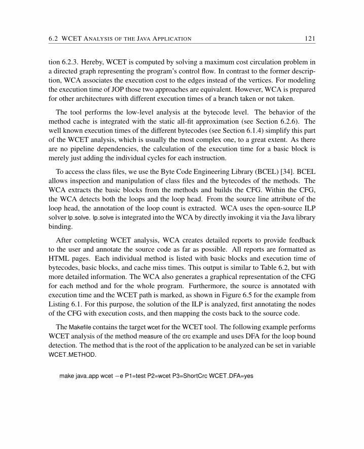
6.2 WCET ANALYSIS OF THE JAVA APPLICATION 121
tion 6.2.3. Hereby, WCET is computed by solving a maximum cost circulation problem ina directed graph representing the program’s control flow. In contrast to the former descrip-tion, WCA associates the execution cost to the edges instead of the vertices. For modelingthe execution time of JOP those two approaches are equivalent. However, WCA is preparedfor other architectures with different execution times of a branch taken or not taken.
The tool performs the low-level analysis at the bytecode level. The behavior of themethod cache is integrated with the static all-fit approximation (see Section 6.2.6). Thewell known execution times of the different bytecodes (see Section 6.1.4) simplify this partof the WCET analysis, which is usually the most complex one, to a great extent. As thereare no pipeline dependencies, the calculation of the execution time for a basic block ismerely just adding the individual cycles for each instruction.
To access the class files, we use the Byte Code Engineering Library (BCEL) [34]. BCELallows inspection and manipulation of class files and the bytecodes of the methods. TheWCA extracts the basic blocks from the methods and builds the CFG. Within the CFG,the WCA detects both the loops and the loop head. From the source line attribute of theloop head, the annotation of the loop count is extracted. WCA uses the open-source ILPsolver lp solve. lp solve is integrated into the WCA by directly invoking it via the Java librarybinding.
After completing WCET analysis, WCA creates detailed reports to provide feedbackto the user and annotate the source code as far as possible. All reports are formatted asHTML pages. Each individual method is listed with basic blocks and execution time ofbytecodes, basic blocks, and cache miss times. This output is similar to Table 6.2, but withmore detailed information. The WCA also generates a graphical representation of the CFGfor each method and for the whole program. Furthermore, the source is annotated withexecution time and the WCET path is marked, as shown in Figure 6.5 for the example fromListing 6.1. For this purpose, the solution of the ILP is analyzed, first annotating the nodesof the CFG with execution costs, and then mapping the costs back to the source code.
The Makefile contains the target wcet for the WCET tool. The following example performsWCET analysis of the method measure of the crc example and uses DFA for the loop bounddetection. The method that is the root of the application to be analyzed can be set in variableWCET METHOD.
make java app wcet −e P1=test P2=wcet P3=ShortCrc WCET DFA=yes
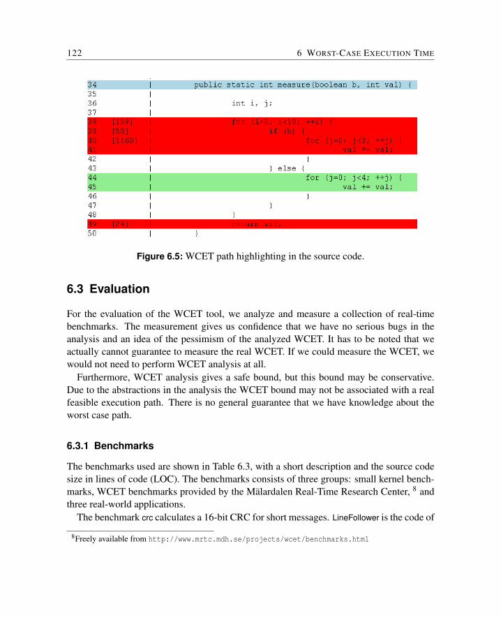
122 6 WORST-CASE EXECUTION TIME
Figure 6.5: WCET path highlighting in the source code.
6.3 Evaluation
For the evaluation of the WCET tool, we analyze and measure a collection of real-timebenchmarks. The measurement gives us confidence that we have no serious bugs in theanalysis and an idea of the pessimism of the analyzed WCET. It has to be noted that weactually cannot guarantee to measure the real WCET. If we could measure the WCET, wewould not need to perform WCET analysis at all.
Furthermore, WCET analysis gives a safe bound, but this bound may be conservative.Due to the abstractions in the analysis the WCET bound may not be associated with a realfeasible execution path. There is no general guarantee that we have knowledge about theworst case path.
6.3.1 Benchmarks
The benchmarks used are shown in Table 6.3, with a short description and the source codesize in lines of code (LOC). The benchmarks consists of three groups: small kernel bench-marks, WCET benchmarks provided by the Malardalen Real-Time Research Center, 8 andthree real-world applications.
The benchmark crc calculates a 16-bit CRC for short messages. LineFollower is the code of
8Freely available from http://www.mrtc.mdh.se/projects/wcet/benchmarks.html
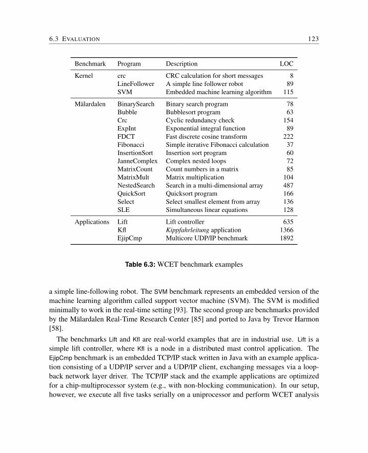
6.3 EVALUATION 123
Benchmark Program Description LOC
Kernel crc CRC calculation for short messages 8LineFollower A simple line follower robot 89SVM Embedded machine learning algorithm 115
Malardalen BinarySearch Binary search program 78Bubble Bubblesort program 63Crc Cyclic redundancy check 154ExpInt Exponential integral function 89FDCT Fast discrete cosine transform 222Fibonacci Simple iterative Fibonacci calculation 37InsertionSort Insertion sort program 60JanneComplex Complex nested loops 72MatrixCount Count numbers in a matrix 85MatrixMult Matrix multiplication 104NestedSearch Search in a multi-dimensional array 487QuickSort Quicksort program 166Select Select smallest element from array 136SLE Simultaneous linear equations 128
Applications Lift Lift controller 635Kfl Kippfahrleitung application 1366EjipCmp Multicore UDP/IP benchmark 1892
Table 6.3: WCET benchmark examples
a simple line-following robot. The SVM benchmark represents an embedded version of themachine learning algorithm called support vector machine (SVM). The SVM is modifiedminimally to work in the real-time setting [93]. The second group are benchmarks providedby the Malardalen Real-Time Research Center [85] and ported to Java by Trevor Harmon[58].
The benchmarks Lift and Kfl are real-world examples that are in industrial use. Lift is asimple lift controller, where Kfl is a node in a distributed mast control application. TheEjipCmp benchmark is an embedded TCP/IP stack written in Java with an example applica-tion consisting of a UDP/IP server and a UDP/IP client, exchanging messages via a loop-back network layer driver. The TCP/IP stack and the example applications are optimizedfor a chip-multiprocessor system (e.g., with non-blocking communication). In our setup,however, we execute all five tasks serially on a uniprocessor and perform WCET analysis
124 6 WORST-CASE EXECUTION TIME
Measured Estimated PessimismProgram (cycles) (cycles) (ratio)
crc 1449 1513 1.04LineFollower 2348 2411 1.03SVM 104880 107009 1.02
BinarySearch 631 636 1.01Bubble 1262717 1815734 1.44Crc 191825 383026 2.00ExpInt 324419 429954 1.33FDCT 19124 19131 1.00Fibonacci 1127 1138 1.01InsertionSort 8927 15410 1.73JanneComplex 886 6991 7.89MatrixCount 16420 16423 1.00MatrixMult 1088497 1088509 1.00NestedSearch 51777 64687 1.25QuickSort 9942 115383 11.61Select 5362 55894 10.42SLE 20408 50514 2.48
Lift 5446 8466 1.55Kfl 10411 39555 3.80EjipCmp 15297 21965 1.44
Table 6.4: Measured and estimated WCET with result in clock cycles
for the aggregation of the five tasks.The configuration of JOP for the evaluation is with a 4 KB method cache configured for
16 blocks. The memory access times are 2 cycles for a read and 3 cycles for a write.
6.3.2 Analysis and Measurements
Table 6.4 shows the measured execution time and the analyzed WCET. The last columngives an idea of the pessimism of the WCET analysis. It has to be noted (again) that weactually cannot guarantee to measure the real WCET. If we could measure the WCET, wewould not need to perform WCET analysis at all. The WCET analysis result of a methodis defined as follows: WCA reports the WCET of the executable code within a method
6.3 EVALUATION 125
including the return statement. The invoke of the to-be-analyzed method is not part of theanalysis. With respect to cache analysis the return from the method does not include anymiss time – invoke and return miss time are considered as part of the invoke instruction. Forthe measurement we use a cycle counter and take a time stamp before the first instructionof the method and after the return from the method.
For very simple programs, such as crc, robot, and SVM the pessimism is quite low. Thesame is true for several of the benchmarks from the Malardalen benchmark suit. Someare almost cycle accurate. The small overestimation of, e.g., 5 cycles for BinarySearch,results from our measurement methodology and the definition of what the WCET of asingle method is. To avoid instrumenting all benchmarks with time stamp code we wrapthe benchmarks in a method measure(), vary which benchmark is invoked in measure(), andanalyze this method. Therefore, measure() contains an invoke and the control is return tomeasure(). In the case of small benchmarks the method cache still contains measure() onthe return from the benchmark method. However, WCA does not include measure() as apossible method for the static method cache analysis (it is performed on a invoke and noinvoke of measure() is seen by WCA). Therefore, the return from the benchmark method isclassified as miss.
The pessimism of most of the other benchmarks, including the two applications Lift andEjipCmp, are in an acceptable range below a factor of 2. Three benchmarks, JanneCom-plex, QuickSort, and Select, stand out with a high pessimism. JanneComplex is an artificialbenchmark with a complex loop dependency of an inner loop and the annotation results in aconservative estimation. However, it has to be noted that the benchmarks from Malardalenare designed to challenge WCET tools. We assume that a safety-critical programmer wouldnot use QuickSort as a first choice for time-predictable code.
The pessimism of Kfl is quite high. The difference between the measurement, and theanalysis in the Kfl example, results from the fact that our measurement does not cover theWCET path. We only simulate input values and commands for the mission phase. However,the main loop of Kfl also handles service functions. Those functions are not part of themission phase, but make up the WCET path. If we omit the non-feasible path to the serviceroutine the WCET drops down to 22875 and the overestimation is 2.2.
The Kfl example show the issue when a real-time application is developed without aWCET analysis tool available. Getting the feedback from the analysis earlier in the de-sign phase can help the programmer to adapt to a WCET aware programming style. Inone extreme, this can end up in the single-path programming style [108]. A less radicalapproach can use some heuristics for a WCET aware programming style. For instance,avoiding the service routines in the application main loop.
The results given in Table 6.4 are comparable to the results presented in [134]. Most
126 6 WORST-CASE EXECUTION TIME
benchmarks now take less cycles than in 2006 as the performance of JOP has been ad-vanced. The exceptions are two benchmarks, LineFollower and Kfl, which now have a higherWCET. The line-following robot example was rewritten in a more object-oriented way. Fi-nally, the different number for the Kfl resulted from a bug in the WCA that was correctedafter the publication in 2006.
6.4 Discussion
We found that the approach of a time-predictable processor and static WCET analysis isa feasible solution for future safety-critical systems. However, there are some remainingquestions that are discussed in the following sections.
6.4.1 On Correctness of WCET Analysis
Safe WCET approximation depends on the correct modeling of the target architecture andthe correct implementation of the analysis tools. During the course of this paper we havefound a bug in the WCA from 2006 and have also found bugs in the low-level timingdescription of JOP. However, the open-source approach for the processor and the toolsincreases the chance that bugs are found. Furthermore, we have compared the results of thenew implementation of WCA with two independent implementations of WCET analysisfor JOP: The Volta project by Trevor Harmon [57] and the former implementation of WCA[134]. The results differ only slightly due to different versions of JOP that Volta, used anda less accurate cache analysis implemented in the second tool. It should be noted that JOPand the WCA are still considered on-going research prototypes for real-time systems. Wewould not (yet) suggest to deploy JOP in the next safety-critical application.
6.4.2 Is JOP the Only Target Architecture?
JOP is the primary low-level target for the WCET analysis tool as it is: (a) a simple proces-sor, (b) open-source, and (c) the execution timing is well-documented (see Appendix D).Furthermore, the JOP design is actually the root of a family of Java processors. FlaviusGruian has built a JOP compatible processor, with a different pipeline organization, withBluespec Verilog [50]. The SHAP Java processor [157], although now with a differentpipeline structure and hardware assisted garbage collection, also has its roots in the JOPdesign. We assume that these processors are also WCET analysis friendly. The questionremains how easy the analysis can be adapted for other Java processors.
6.4 DISCUSSION 127
The same analysis is not possible for other Java processors. Either the information on thebytecode execution time is missing9 or some processor features (e.g., the high variabilityof the latency for a trap in picoJava) would result in very conservative WCET estimates.Another example that prohibits exact analysis is the mechanism to automatically fill andspill the stack cache in picoJava [145, 146]. The time when the memory (cache) is occupiedby this spill/fill action depends on a long instruction history. Also the fill level of the 16-byte-deep prefetch buffer, which is needed for instruction folding, depends on the executionhistory. All these automatic buffering features have to be modeled quite conservatively. Apragmatic solution is to assume empty buffers at the start of a basic block. As basic blocksare quite short, most of the buffering/prefetching does not help to lower the WCET.
Only for the Cjip processor is the execution time well documented [69]. However, themeasured execution time of some bytecodes is higher than the documented values [123].Therefore the documentation is not complete to provide a safe processor model of the Cjipfor WCET analysis.
The real-time Java processor jamuth [149] is a possible target for the WCA. There ison-going work with Sascha Uhrig to integrate the timing model of jamuth into the WCA. Apreliminary version of that model has been tested. The analysis tool need to be changed tomodel a few pipeline dependencies.
Still, WCET analysis of Java programs on RISC processors with a compiling JVM is achallenge. With a compiling JVM, the WCET friendly bytecodes are further compiled intomachine code. Information is lost in the second transformation. This is not the case with adedicated Java processor such as JOP.
6.4.3 Object-oriented Evaluation Examples
Most of the benchmarks used are written in a rather conservative programming style. TheMalardalen benchmarks are small kernels that do not stress the cache analysis. We wouldlike to use more object-oriented real-time examples for the evaluation. Then, we can eval-uate if object-oriented programming style with dynamic method dispatch and rather smallmethods is a feasible option for future real-time systems.
6.4.4 WCET Analysis for Chip-multiprocessors
Chip-multiprocessors (CMP) are now considered as the future technology for high-performance embedded systems. Christof Pitter has built a CMP version of JOP thatincludes a time-predictable memory arbiter [97]. During the course of his thesis he has
9We tried hard to get this information for the aJile processor.
128 6 WORST-CASE EXECUTION TIME
adapted the low-level timing calculation of the WCET tool to integrate the memory accesstimes with the time-sliced arbiter. Therefore, it is possible to derive WCET values for tasksrunning on a CMP system with shared main memory. To best of our knowledge, this is thefirst time-predictable CMP system where WCET analysis is available.
The first estimation of bytecode timings for the CMP system considers only individualbytecodes. However, with variable memory access times due to memory arbitration thisestimate is conservative. An extension to basic block analysis and using model checkingto analyze possible interactions between the memory arbitration process and the programexecution should result in tighter WCET estimates.
The JOP CMP system showed the importance of tighter method cache analysis. Com-pared to the simple approach of the original WCA tool, the new static cache approximationyielded in 15% tighter WCET estimates for a 8 core CMP system.
6.4.5 Co-Development of Processor Architecture and WCET Analysis
JOP is an example of a time-predictable computer architecture. An extension of this ap-proach to RISC and VLIW based processors is presented in [132]. We consider a co-development of time-predictable computer architecture and WCET analysis for the archi-tectural features as an ideal approach for future real-time systems. A new time-predictablefeature (e.g., a data cache organization) can only be evaluated when the analysis is avail-able. The analysis, and what can be analyzed within practical execution time and memorydemands, shall guide the computer architect of future time-predictable processors.
6.4.6 Further Paths to Explore
The combination of a bytecode based optimizer (a prototype is available as part of the JOPsources) with WCET analysis can be applied to minimize the WCET path. The optimizercan be guided by the results from the application. This iterative flow can be used to mini-mize the worst-case path instead of the average-case path in the application.
6.5 Summary
In this chapter, the WCET analysis tool based on the ILP approach has been presented. Thearchitecture of the Java processor greatly simplifies the low-level part of WCET analysis, asit can be performed at the Java bytecode level. An instruction cache, named method cache,stores complete methods, and is integrated into the WCET analysis tool.
6.6 FURTHER READING 129
The WCET analysis tool, with the help of DFA detected loop bounds, provides WCETvalues for the schedulability analysis. Complex loops still need to be annotated in thesource. A receiver type analysis helps to tighten the WCET of object-oriented programs.We have also integrated the method cache into the analysis. The cache can be analyzed atthe method level and does not need the full program CFG. Besides the calculation of theWCET, the tool provides user feedback by generating bytecode listings with timing infor-mation and a graphical representation of the CFG with timing and frequency information.This representation of the WCET path through the code can guide the developer to writeWCET aware real-time code.
The experiments with the WCET analyzer tool have demonstrated that we have achievedour goal: JOP is a simple target for WCET analysis. Most bytecodes have a single executiontime (WCET = BCET), and the WCET of a task (the analysis at the bytecode level) dependsonly on the control flow. No pipeline or data dependencies complicate the low-level part ofWCET analysis.
6.6 Further Reading
There are a lot of papers available on WCET analysis and modeling of low-level processorfeatures. This section gives an overview of the related work for our WCET analyzer.
6.6.1 WCET Analysis
Shaw presents in [139] timing schemas to calculate minimum and maximum executiontime for common language constructs. The rules allow to collapse the CFG of a programuntil a final single value represents the WCET. However, with this approach it is not straightforward to incorporate global low-level attributes, such as pipelines or caches. The resultingbounds are not tight enough to be practically useful.
Computing the WCET with an integer linear programming (ILP) solver is proposed in[110] and [79]. The approach is named graph-based and implicit path enumeration respec-tively. We base our WCET analyzer on the ideas from these two groups.
The WCET is calculated by transforming the calculation to an integer linear program-ming problem. Each basic block10 is represented by an edge ei in the T-graph (timinggraph) with the weight of the execution time of the basic block. Vertices vi in the graphrepresent the split and join points in the control flow. Furthermore, each edge is also as-signed an execution frequency fi. The constraints resulting from the T-graph and additional
10A basic block is a sequence of instructions without any jumps or jump targets within this sequence.
130 6 WORST-CASE EXECUTION TIME
functional constraints (e.g. loop bounds) are solved by an ILP solver. The T-graph is similarto a CFG, where the execution time is modeled in the vertices. The motivation to model theexecution time in the edges results from the observation that most basic blocks end with aconditional branch. A conditional branch usually has a different execution time, dependingon whether it is taken or not. This difference is represented by two edges with differentweights.
In [79] a similar approach with ILP is proposed. However, they use the CFG as the basisto build the ILP problem. The approach is extended to model the instruction cache withcache conflict graphs. The evaluation with an Intel i960 processor shows tight results forsmall programs [80]. However, the conservative modeling of the register window (over-flow/underflow on each function call/return) adds 50 cycles to each call and return. Thisobservation is another argument for a WCET aware processor architecture.
WCET analysis of object-oriented languages is presented by Gustafsson [51]. Gustafssonuses abstract interpretation for automatic flow analysis to find loop bounds and in feasiblepaths. The work is extended to a modular WCET tool with instruction cache analysis andpipeline analysis [43]. A summary of new complexities to WCET analysis is given in [52].
Cache memories for the instructions and data are classic examples of the paradigm: Makethe common case fast. Avoiding or ignoring this feature in real-time systems, due to itsunpredictable behavior, results in a very pessimistic WCET bound. Plenty of effort has goneinto research to integrate the instruction cache into the timing analysis of tasks [11, 60],the cache’s influence on task preemption [78, 31], and integration of the cache analysiswith the pipeline analysis [59]. Heckmann et. al described the influence of different cachearchitectures on WCET analysis [61].
An overview of WCET related research is presented in [107] and [152].
6.6.2 WCET Analysis for Java
WCET analysis at the bytecode level became a research topic, at the time Java was consid-ered for future real-time systems. WCET analysis at the bytecode level was first consideredin [23]. It is argued that the well formed intermediate representation of a program in Javabytecode, which can also be generated from compilers for other languages (e.g. Ada), iswell suited for a portable WCET analysis tool. In that paper, annotations for Java and Adaare presented to guide WCET analysis at bytecode level. The work is extended to addressthe machine-dependent low-level timing analysis [21]. Worst-case execution frequenciesof Java bytecodes are introduced for a machine independent timing information. Pipelineeffects (on the target machine) across bytecode boundaries are modeled by a gain time forbytecode pairs.
6.6 FURTHER READING 131
In [106] a portable WCET analysis is proposed. The abstract WCET analysis is per-formed on the development site and generates abstract WCET information. The concreteWCET analysis is performed on the target machine by replacing abstract values within theWCET formulae by the machine dependent concrete values.
In [22], an extension of [23] and [21], an approach how the portable WCET informationcan be embedded in the Java class file is given. It is suggested that the final WCET calcula-tion is performed by the target JVM. The calculation is performed for each method and thestatic call tree is traversed by a recursive call of the WCET analyzer.
6.6.3 WCET Analysis for JOP
A strong indication that JOP is a WCET friendly design, are that other real-time analysisprojects use JOP as the primary target platform. The first IPET based WCET analysistool that includes the timing model of JOP is presented in [134]. A simplified version ofthe method cache, the two block cache, is analyzed for invocations in inner loops. TrevorHarmon developed a tree-based WCET analyzer for interactive back-annotation of WCETestimates into the program source [57, 56]. The tool is extended to integrate JOP’s twoblock method cache [58]. Model checking is used to analyze the timing and schedulingproperties of a complete application within a single model [24]. However, even with asimple example, consisting of two periodic and two sporadic tasks, this approach leads to avery long analysis time. In contrast to that approach our opinion is that a combined WCETanalysis and schedulability analysis is infeasible for non-trivial applications. Therefore,we stay in the WCET analysis domain, and consider the well established schedulabilityanalysis as an extra step.
Compared to those three tools, which also target JOP, our presented WCET tool is en-hanced with: (a) analysis of bytecodes that are implemented in Java; (b) integration ofdata-flow analysis for loop bounds and receiver methods; (c) a tighter IPET based methodcache analysis; and (d) an evaluation of model checking for exact modeling of the methodcache.

7 Real-Time Garbage Collection
Automatic memory management or garbage collection greatly simplifies development oflarge systems. However, garbage collection is usually not used in real-time systems due tothe unpredictable temporal behavior of current implementations of a garbage collector. Inthis chapter we describe a concurrent collector that is scheduled periodically in the sameway as ordinary application threads. We provide an upper bound for the collector periodso that the application threads will never run out of memory. This chapter is based onfollowing papers: [124, 138, 135].
7.1 Introduction
Garbage Collection (GC) is an essential part of the Java runtime system. GC enables au-tomatic dynamic memory management which is essential to build large applications. Au-tomatic memory management frees the programmer from complex and error prone explicitmemory management (malloc and free).
However, garbage collection is considered unsuitable for real-time systems due to the un-predictable blocking times introduced by the GC work. One solution, used in the Real-TimeSpecification for Java (RTSJ) [25], introduces new thread types with program-managed,scoped memory for dynamic memory requirements. This scoped memory (and static mem-ory called immortal memory) is not managed by the GC, and strict assignment rules be-tween different memory areas have to be checked at runtime. This programming modeldiffers largely from standard Java and is difficult to use [87, 101].
We believe that for the acceptance of Java for real-time systems, the restrictions imposedby the RTSJ are too strong. To simplify creation of possible large real-time applications,most of the code should be able to use the GC managed heap. For a collector to be used inreal-time systems two points are essential:
• The GC has to be incremental with a short maximum blocking time that has to beknown
• The GC has to keep up with the garbage generated by the application threads to avoidout-of-memory stalls
134 7 REAL-TIME GARBAGE COLLECTION
The first point is necessary to limit interference between the GC thread and high-prioritythreads. It is also essential to minimize the overhead introduced by read- and write-barriers,which are necessary for synchronization between the GC thread and the application threads.The design of a GC within these constraints is the topic of this chapter.
The second issue that has to be considered is scheduling the GC so that the GC collectsenough garbage. The memory demands (static and dynamic) by the application threadshave to be analyzed. These requirements, together with the properties of the GC, resultin scheduling parameters for the GC thread. We will provide a solution to calculate themaximum period of the GC thread that will collect enough memory in each collector cycleso we will never run out of memory. The collector cycle depends on the heap size and theallocation rate of the application threads.
To distinguish between other garbage collectors and a collector for (hard) real-time sys-tems we define a real-time collector as follows:
A real-time garbage collector provides time predictable automatic memorymanagement for tasks with a bounded memory allocation rate with minimaltemporal interference to tasks that use only static memory.
The collector presented in this chapter is based on the work by Steele [142], Dijkstra [38]and Baker [19]. However, the copying collector is changed to perform the copy of an objectconcurrently by the collector and not as part of the mutator work. Therefore we name itconcurrent-copy collector.
We will use the terms first introduced by Dijkstra with his On-the-Fly concurrent col-lector [38]. The application is called the mutator to reinforce that the application changes(mutates) the object graph while the GC does the collection work. The GC process is simplycalled collector. In the following discussion we will use the color scheme of white, gray,and black objects:
Black indicates that the object and all immediate descendants have been visited by thecollector.
Grey objects have been visited, but the descendants may not have been visited by the col-lector, or the mutator has changed the object.
White objects are unvisited. At the beginning of a GC cycle all objects are white. At theend of the tracing, all white objects are garbage.
At the end of a collection cycle all black objects are live (or floating garbage) and allwhite objects are garbage.
7.1 INTRODUCTION 135
7.1.1 Incremental Collection
An incremental collector can be realized in two ways: either by doing part of the work oneach allocation of a new object or by running the collector as an independent process. Fora single-threaded application, the first method is simpler as less synchronization betweenthe application and the collector is necessary. For a multi-threaded environment there isno advantage by interleaving collector work with object allocation. In this case we needsynchronization between the collector work done by one thread and the manipulation of theobject graph performed by the other mutator thread. Therefore we will consider a concur-rent solution where the collector runs in its own thread or processor. It is even possible torealize the collector as dedicated hardware [49].
7.1.2 Conservatism
Incremental collector algorithms are conservative, meaning that objects becoming unreach-able during collection are not collected by the collector — they are floating garbage. Manyapproaches exist to reduce this conservatism in the general case. However, algorithms thatcompletely avoid floating garbage are impractical. For different conservative collectors theworst-case bounds are all the same (i.e., all objects that become unreachable during col-lection remain floating garbage). Therefore the level of conservatism is not an issue forreal-time collectors.
7.1.3 Safety Critical Java
In [137] a profile for safety critical Java (SCJ) is defined. SCJ has two interesting propertiesthat may simplify the implementation of a real-time collector. Firstly, the split betweeninitialization and mission phase, and secondly the simplified threading model (which alsomandates that self-blocking operations are illegal in the mission phase). During initializa-tion of the application a SCJ virtual machine does not have to meet any real-time constraints(other than possibly a worst case bound on the entire initialization phase). It is perfectlyacceptable to use a non-real-time GC implementation during this phase – even a stop-the-world GC. As the change from initialization to mission phase is explicit, it is clear when thevirtual machine must initiate real-time collection and which code runs during the missionphase.
Simplifying the threading model has the following advantage, if the collector thread runsat a lower priority than all other threads in the system, it is the case that when it runs allother threads have returned from their calls to run(). This is trivially true due to the priority
136 7 REAL-TIME GARBAGE COLLECTION
preemptive scheduling discipline.1 Any thread that has not returned from its run() methodwill preempt the GC until it returns. This has the side effect that the GC will never see aroot in the call stack of another thread. Therefore, the usually atomic operation of scanningcall stacks can be omitted in the mission phase. We will elaborate on this property inSection 7.3.
7.2 Scheduling of the Collector Thread
The collector work can be scheduled either work based or time based. On a work basedscheduling, as performed in [140], an incremental part of the collector work is performed atobject allocation. This approach sounds quite natural as threads that allocate more objectshave to pay for the collector work. Furthermore, no additional collector thread is necessary.The main issue with this approach is to determine how much work has to be done on eachallocation – a non trivial question as collection work consists of different phases. A moresubtle question is: Why should a high frequency (and high priority) thread increase itsWCET by performing collector work that does not have to be done at that period? Leavingthe collector work to a thread with a longer period allows higher utilization of the system.
On a time based scheduling of the collector work, the collector runs in its own thread.Scheduling this thread as a normal real-time thread is quite natural for a hard real-timesystem. The question is: which priority to assign to the collector thread? The Metronomecollector [18] uses the highest priority for the collector. Robertz and Henriksson [113] andSchoeberl [124] argue for the lowest priority. When building hard real-time systems theanswer must take scheduling theory into consideration: the priority is assigned according tothe period, either rate monotonic [83] or more general deadline monotonic [13]. Assumingthat the period of the collector is the longest in the system and the deadline equals the periodthe collector gets the lowest priority.
In this section we provide an upper bound for the collector period so that the applica-tion threads will never run out of memory. The collector period, besides the WCET ofthe collector, is the single parameter of the collector that can be incorporated in standardschedulability analysis.
The following symbols are used in this section: heap size for a mark-compact collector(HMC) and for a concurrent-copying collector (HCC) containing both semi-spaces, period ofthe GC thread (TGC), period of a single mutator thread (TM), period of mutator thread i (Ti)from a set of threads, and memory amount allocated by a single mutator (a) or by mutator i(ai) from a set of threads.
1If we would allow blocking in the application threads, we would also need to block the GC thread.
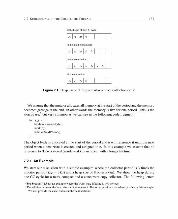
7.2 SCHEDULING OF THE COLLECTOR THREAD 137
l7f6f5f4
after compaction
l7f6f5f4
before compaction
g3g2g1
l5f4
in the middle (marking)
g1 g2 g3
g1 g2 g3 l4
at the begin of the GC cycle
Figure 7.1: Heap usage during a mark-compact collection cycle
We assume that the mutator allocates all memory at the start of the period and the memorybecomes garbage at the end. In other words the memory is live for one period. This is theworst-case,2 but very common as we can see in the following code fragment.
for (;;) {Node n = new Node();work(n);waitForNextPeriod();
}
The object Node is allocated at the start of the period and n will reference it until the nextperiod when a new Node is created and assigned to n. In this example we assume that noreference to Node is stored (inside work) to an object with a longer lifetime.
7.2.1 An Example
We start our discussion with a simple example3 where the collector period is 3 times themutator period (TGC = 3TM) and a heap size of 8 objects (8a). We show the heap duringone GC cycle for a mark-compact and a concurrent-copy collector. The following letters
2See Section 7.2.3 for an example where the worst-case lifetime is two periods.3The relation between the heap size and the mutator/collector proportion is an arbitrary value in this example.
We will provide the exact values in the next sections.
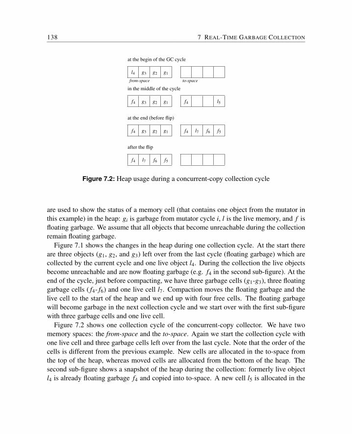
138 7 REAL-TIME GARBAGE COLLECTION
l5f4
f5f6l7f4
g1g2g3f4
in the middle of the cycle
g1g2g3f4
at the end (before flip)
f4 l7 f6 f5
after the flip
to-space
at the begin of the GC cycle
from-space
l4 g3 g2 g1
Figure 7.2: Heap usage during a concurrent-copy collection cycle
are used to show the status of a memory cell (that contains one object from the mutator inthis example) in the heap: gi is garbage from mutator cycle i, l is the live memory, and f isfloating garbage. We assume that all objects that become unreachable during the collectionremain floating garbage.
Figure 7.1 shows the changes in the heap during one collection cycle. At the start thereare three objects (g1, g2, and g3) left over from the last cycle (floating garbage) which arecollected by the current cycle and one live object l4. During the collection the live objectsbecome unreachable and are now floating garbage (e.g. f4 in the second sub-figure). At theend of the cycle, just before compacting, we have three garbage cells (g1-g3), three floatinggarbage cells ( f4- f6) and one live cell l7. Compaction moves the floating garbage and thelive cell to the start of the heap and we end up with four free cells. The floating garbagewill become garbage in the next collection cycle and we start over with the first sub-figurewith three garbage cells and one live cell.
Figure 7.2 shows one collection cycle of the concurrent-copy collector. We have twomemory spaces: the from-space and the to-space. Again we start the collection cycle withone live cell and three garbage cells left over from the last cycle. Note that the order of thecells is different from the previous example. New cells are allocated in the to-space fromthe top of the heap, whereas moved cells are allocated from the bottom of the heap. Thesecond sub-figure shows a snapshot of the heap during the collection: formerly live objectl4 is already floating garbage f4 and copied into to-space. A new cell l5 is allocated in the
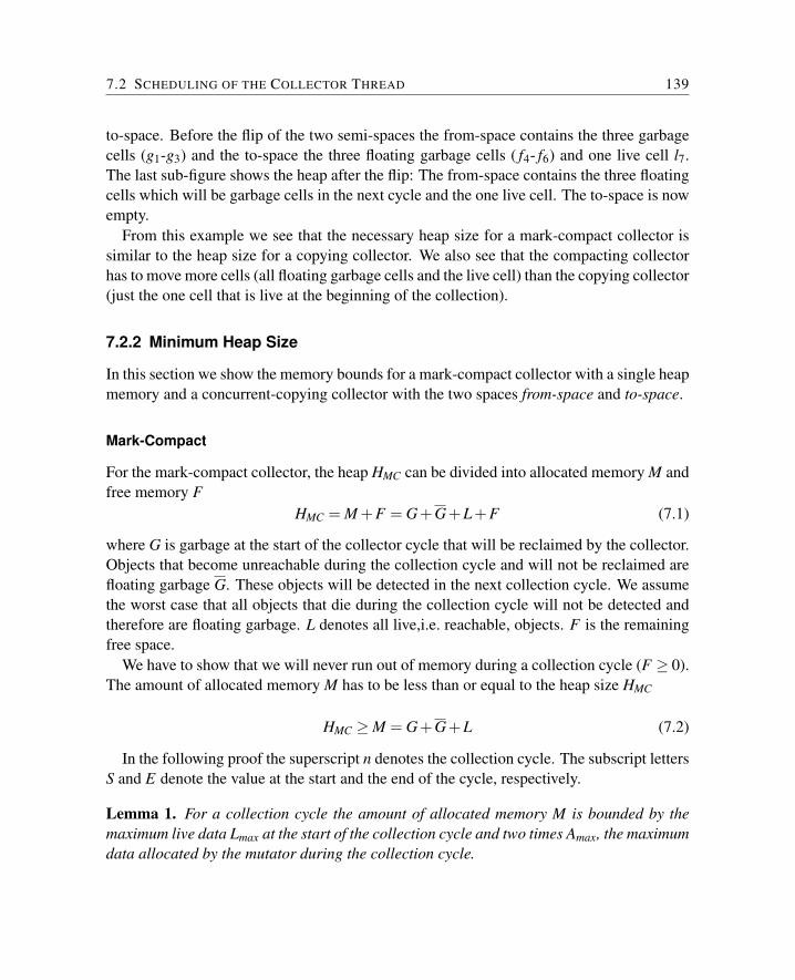
7.2 SCHEDULING OF THE COLLECTOR THREAD 139
to-space. Before the flip of the two semi-spaces the from-space contains the three garbagecells (g1-g3) and the to-space the three floating garbage cells ( f4- f6) and one live cell l7.The last sub-figure shows the heap after the flip: The from-space contains the three floatingcells which will be garbage cells in the next cycle and the one live cell. The to-space is nowempty.
From this example we see that the necessary heap size for a mark-compact collector issimilar to the heap size for a copying collector. We also see that the compacting collectorhas to move more cells (all floating garbage cells and the live cell) than the copying collector(just the one cell that is live at the beginning of the collection).
7.2.2 Minimum Heap Size
In this section we show the memory bounds for a mark-compact collector with a single heapmemory and a concurrent-copying collector with the two spaces from-space and to-space.
Mark-Compact
For the mark-compact collector, the heap HMC can be divided into allocated memory M andfree memory F
HMC = M +F = G+G+L+F (7.1)
where G is garbage at the start of the collector cycle that will be reclaimed by the collector.Objects that become unreachable during the collection cycle and will not be reclaimed arefloating garbage G. These objects will be detected in the next collection cycle. We assumethe worst case that all objects that die during the collection cycle will not be detected andtherefore are floating garbage. L denotes all live,i.e. reachable, objects. F is the remainingfree space.
We have to show that we will never run out of memory during a collection cycle (F ≥ 0).The amount of allocated memory M has to be less than or equal to the heap size HMC
HMC ≥M = G+G+L (7.2)
In the following proof the superscript n denotes the collection cycle. The subscript lettersS and E denote the value at the start and the end of the cycle, respectively.
Lemma 1. For a collection cycle the amount of allocated memory M is bounded by themaximum live data Lmax at the start of the collection cycle and two times Amax, the maximumdata allocated by the mutator during the collection cycle.
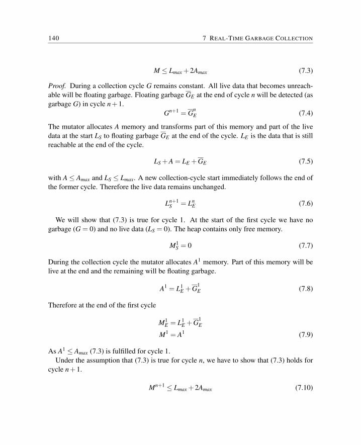
140 7 REAL-TIME GARBAGE COLLECTION
M ≤ Lmax +2Amax (7.3)
Proof. During a collection cycle G remains constant. All live data that becomes unreach-able will be floating garbage. Floating garbage GE at the end of cycle n will be detected (asgarbage G) in cycle n+1.
Gn+1 = GnE (7.4)
The mutator allocates A memory and transforms part of this memory and part of the livedata at the start LS to floating garbage GE at the end of the cycle. LE is the data that is stillreachable at the end of the cycle.
LS +A = LE +GE (7.5)
with A≤ Amax and LS ≤ Lmax. A new collection-cycle start immediately follows the end ofthe former cycle. Therefore the live data remains unchanged.
Ln+1S = Ln
E (7.6)
We will show that (7.3) is true for cycle 1. At the start of the first cycle we have nogarbage (G = 0) and no live data (LS = 0). The heap contains only free memory.
M1S = 0 (7.7)
During the collection cycle the mutator allocates A1 memory. Part of this memory will belive at the end and the remaining will be floating garbage.
A1 = L1E +G1
E (7.8)
Therefore at the end of the first cycle
M1E = L1
E +G1E
M1 = A1 (7.9)
As A1 ≤ Amax (7.3) is fulfilled for cycle 1.Under the assumption that (7.3) is true for cycle n, we have to show that (7.3) holds for
cycle n+1.
Mn+1 ≤ Lmax +2Amax (7.10)
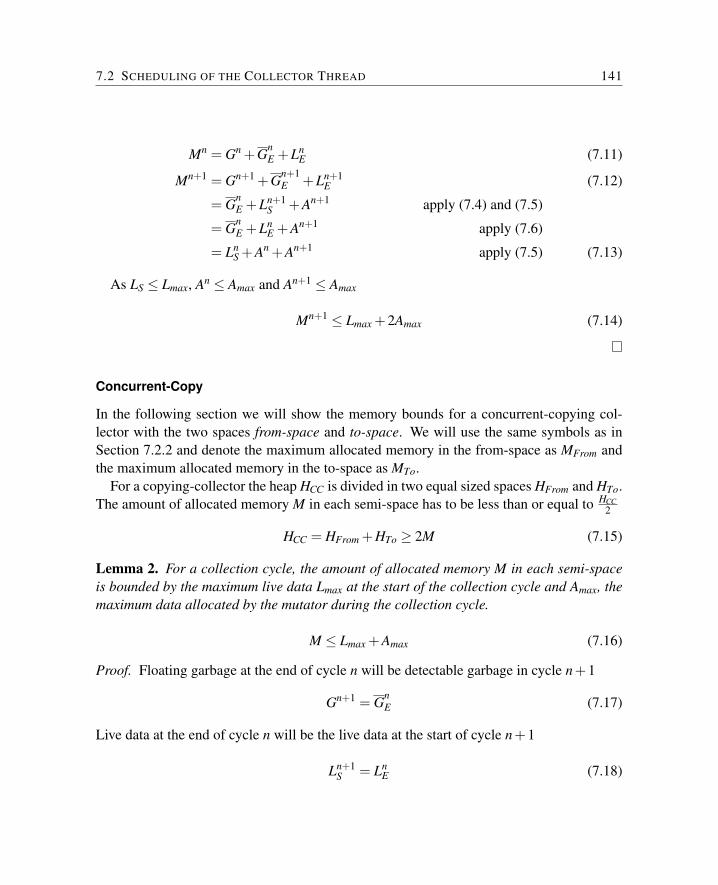
7.2 SCHEDULING OF THE COLLECTOR THREAD 141
Mn = Gn +GnE +Ln
E (7.11)
Mn+1 = Gn+1 +Gn+1E +Ln+1
E (7.12)
= GnE +Ln+1
S +An+1 apply (7.4) and (7.5)
= GnE +Ln
E +An+1 apply (7.6)
= LnS +An +An+1 apply (7.5) (7.13)
As LS ≤ Lmax, An ≤ Amax and An+1 ≤ Amax
Mn+1 ≤ Lmax +2Amax (7.14)
Concurrent-Copy
In the following section we will show the memory bounds for a concurrent-copying col-lector with the two spaces from-space and to-space. We will use the same symbols as inSection 7.2.2 and denote the maximum allocated memory in the from-space as MFrom andthe maximum allocated memory in the to-space as MTo.
For a copying-collector the heap HCC is divided in two equal sized spaces HFrom and HTo.The amount of allocated memory M in each semi-space has to be less than or equal to HCC
2
HCC = HFrom +HTo ≥ 2M (7.15)
Lemma 2. For a collection cycle, the amount of allocated memory M in each semi-spaceis bounded by the maximum live data Lmax at the start of the collection cycle and Amax, themaximum data allocated by the mutator during the collection cycle.
M ≤ Lmax +Amax (7.16)
Proof. Floating garbage at the end of cycle n will be detectable garbage in cycle n+1
Gn+1 = GnE (7.17)
Live data at the end of cycle n will be the live data at the start of cycle n+1
Ln+1S = Ln
E (7.18)
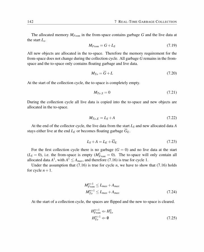
142 7 REAL-TIME GARBAGE COLLECTION
The allocated memory MFrom in the from-space contains garbage G and the live data atthe start Ls.
MFrom = G+LS (7.19)
All new objects are allocated in the to-space. Therefore the memory requirement for thefrom-space does not change during the collection cycle. All garbage G remains in the from-space and the to-space only contains floating garbage and live data.
MTo = G+L (7.20)
At the start of the collection cycle, the to-space is completely empty.
MTo S = 0 (7.21)
During the collection cycle all live data is copied into the to-space and new objects areallocated in the to-space.
MTo E = LS +A (7.22)
At the end of the collector cycle, the live data from the start LS and new allocated data Astays either live at the end LE or becomes floating garbage GE .
LS +A = LE +GE (7.23)
For the first collection cycle there is no garbage (G = 0) and no live data at the start(LS = 0), i.e. the from-space is empty (M1
From = 0). The to-space will only contain allallocated data A1, with A1 ≤ Amax, and therefore (7.16) is true for cycle 1.
Under the assumption that (7.16) is true for cycle n, we have to show that (7.16) holdsfor cycle n+1.
Mn+1From ≤ Lmax +Amax
Mn+1To ≤ Lmax +Amax (7.24)
At the start of a collection cycle, the spaces are flipped and the new to-space is cleared.
Hn+1From⇐ Hn
To
Hn+1To ⇐ /0 (7.25)
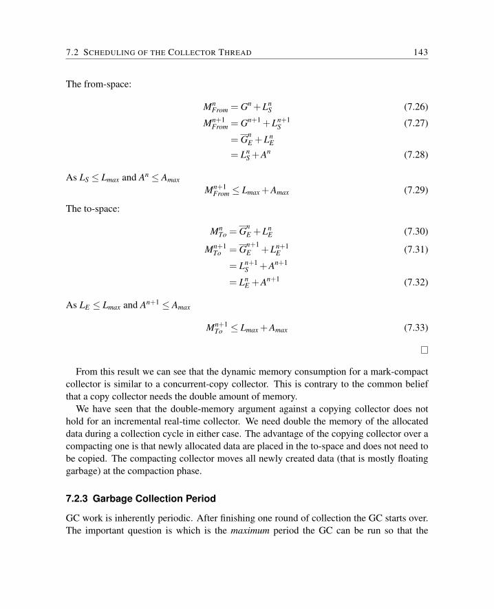
7.2 SCHEDULING OF THE COLLECTOR THREAD 143
The from-space:
MnFrom = Gn +Ln
S (7.26)
Mn+1From = Gn+1 +Ln+1
S (7.27)
= GnE +Ln
E
= LnS +An (7.28)
As LS ≤ Lmax and An ≤ Amax
Mn+1From ≤ Lmax +Amax (7.29)
The to-space:
MnTo = Gn
E +LnE (7.30)
Mn+1To = Gn+1
E +Ln+1E (7.31)
= Ln+1S +An+1
= LnE +An+1 (7.32)
As LE ≤ Lmax and An+1 ≤ Amax
Mn+1To ≤ Lmax +Amax (7.33)
From this result we can see that the dynamic memory consumption for a mark-compactcollector is similar to a concurrent-copy collector. This is contrary to the common beliefthat a copy collector needs the double amount of memory.
We have seen that the double-memory argument against a copying collector does nothold for an incremental real-time collector. We need double the memory of the allocateddata during a collection cycle in either case. The advantage of the copying collector over acompacting one is that newly allocated data are placed in the to-space and does not need tobe copied. The compacting collector moves all newly created data (that is mostly floatinggarbage) at the compaction phase.
7.2.3 Garbage Collection Period
GC work is inherently periodic. After finishing one round of collection the GC starts over.The important question is which is the maximum period the GC can be run so that the
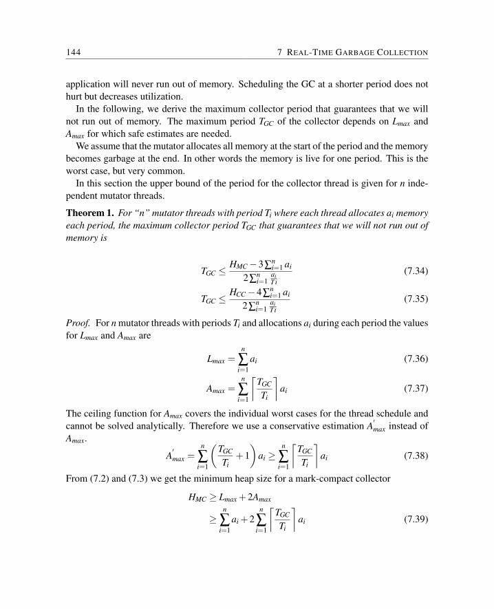
144 7 REAL-TIME GARBAGE COLLECTION
application will never run out of memory. Scheduling the GC at a shorter period does nothurt but decreases utilization.
In the following, we derive the maximum collector period that guarantees that we willnot run out of memory. The maximum period TGC of the collector depends on Lmax andAmax for which safe estimates are needed.
We assume that the mutator allocates all memory at the start of the period and the memorybecomes garbage at the end. In other words the memory is live for one period. This is theworst case, but very common.
In this section the upper bound of the period for the collector thread is given for n inde-pendent mutator threads.
Theorem 1. For “n” mutator threads with period Ti where each thread allocates ai memoryeach period, the maximum collector period TGC that guarantees that we will not run out ofmemory is
TGC ≤HMC−3∑
ni=1 ai
2∑ni=1
aiTi
(7.34)
TGC ≤HCC−4∑
ni=1 ai
2∑ni=1
aiTi
(7.35)
Proof. For n mutator threads with periods Ti and allocations ai during each period the valuesfor Lmax and Amax are
Lmax =n
∑i=1
ai (7.36)
Amax =n
∑i=1
⌈TGC
Ti
⌉ai (7.37)
The ceiling function for Amax covers the individual worst cases for the thread schedule andcannot be solved analytically. Therefore we use a conservative estimation A
′max instead of
Amax.
A′max =
n
∑i=1
(TGC
Ti+1)
ai ≥n
∑i=1
⌈TGC
Ti
⌉ai (7.38)
From (7.2) and (7.3) we get the minimum heap size for a mark-compact collector
HMC ≥ Lmax +2Amax
≥n
∑i=1
ai +2n
∑i=1
⌈TGC
Ti
⌉ai (7.39)
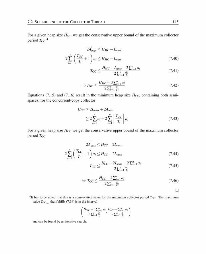
7.2 SCHEDULING OF THE COLLECTOR THREAD 145
For a given heap size HMC we get the conservative upper bound of the maximum collectorperiod TGC
4
2A′max ≤ HMC−Lmax
2n
∑i=1
(TGC
Ti+1)
ai ≤ HMC−Lmax (7.40)
TGC ≤HMC−Lmax−2∑
ni=1 ai
2∑ni=1
aiTi
(7.41)
⇒ TGC ≤HMC−3∑
ni=1 ai
2∑ni=1
aiTi
(7.42)
Equations (7.15) and (7.16) result in the minimum heap size HCC, containing both semi-spaces, for the concurrent-copy collector
HCC ≥ 2Lmax +2Amax
≥ 2n
∑i=1
ai +2n
∑i=1
⌈TGC
Ti
⌉ai (7.43)
For a given heap size HCC we get the conservative upper bound of the maximum collectorperiod TGC
2A′max ≤ HCC−2Lmax
2n
∑i=1
(TGC
Ti+1)
ai ≤ HCC−2Lmax (7.44)
TGC ≤HCC−2Lmax−2∑
ni=1 ai
2∑ni=1
aiTi
(7.45)
⇒ TGC ≤HCC−4∑
ni=1 ai
2∑ni=1
aiTi
(7.46)
4It has to be noted that this is a conservative value for the maximum collector period TGC. The maximumvalue TGCmax that fulfills (7.39) is in the interval(
HMC−3∑ni=1 ai
2∑ni=1
aiTi
,HMC−∑
ni=1 ai
2∑ni=1
aiTi
)and can be found by an iterative search.
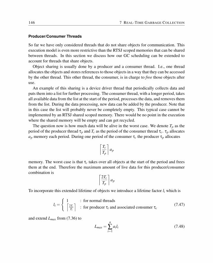
146 7 REAL-TIME GARBAGE COLLECTION
Producer/Consumer Threads
So far we have only considered threads that do not share objects for communication. Thisexecution model is even more restrictive than the RTSJ scoped memories that can be sharedbetween threads. In this section we discuss how our GC scheduling can be extended toaccount for threads that share objects.
Object sharing is usually done by a producer and a consumer thread. I.e., one threadallocates the objects and stores references to those objects in a way that they can be accessedby the other thread. This other thread, the consumer, is in charge to free those objects afteruse.
An example of this sharing is a device driver thread that periodically collects data andputs them into a list for further processing. The consumer thread, with a longer period, takesall available data from the list at the start of the period, processes the data, and removes themfrom the list. During the data processing, new data can be added by the producer. Note thatin this case the list will probably never be completely empty. This typical case cannot beimplemented by an RTSJ shared scoped memory. There would be no point in the executionwhere the shared memory will be empty and can get recycled.
The question now is how much data will be alive in the worst case. We denote Tp as theperiod of the producer thread τp and Tc as the period of the consumer thread τc. τp allocatesap memory each period. During one period of the consumer τc the producer τp allocates⌈
Tc
Tp
⌉ap
memory. The worst case is that τc takes over all objects at the start of the period and freesthem at the end. Therefore the maximum amount of live data for this producer/consumercombination is ⌈
2Tc
Tp
⌉ap
To incorporate this extended lifetime of objects we introduce a lifetime factor li which is
li =
{1 : for normal threads⌈
2TcTi
⌉: for producer τi and associated consumer τc
(7.47)
and extend Lmax from (7.36) to
Lmax =n
∑i=1
aili (7.48)
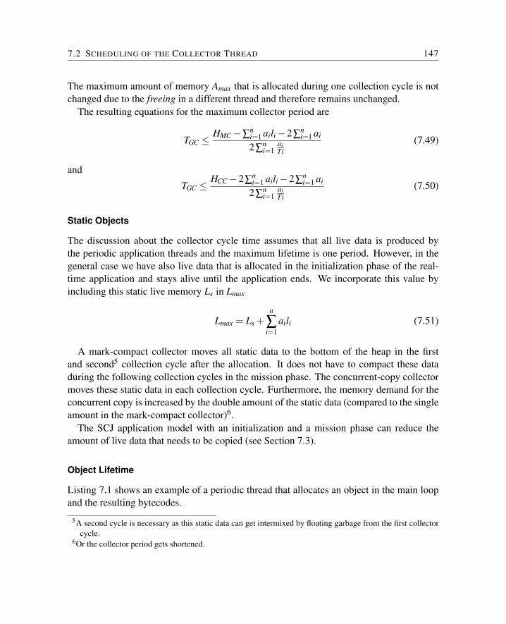
7.2 SCHEDULING OF THE COLLECTOR THREAD 147
The maximum amount of memory Amax that is allocated during one collection cycle is notchanged due to the freeing in a different thread and therefore remains unchanged.
The resulting equations for the maximum collector period are
TGC ≤HMC−∑
ni=1 aili−2∑
ni=1 ai
2∑ni=1
aiTi
(7.49)
and
TGC ≤HCC−2∑
ni=1 aili−2∑
ni=1 ai
2∑ni=1
aiTi
(7.50)
Static Objects
The discussion about the collector cycle time assumes that all live data is produced bythe periodic application threads and the maximum lifetime is one period. However, in thegeneral case we have also live data that is allocated in the initialization phase of the real-time application and stays alive until the application ends. We incorporate this value byincluding this static live memory Ls in Lmax
Lmax = Ls +n
∑i=1
aili (7.51)
A mark-compact collector moves all static data to the bottom of the heap in the firstand second5 collection cycle after the allocation. It does not have to compact these dataduring the following collection cycles in the mission phase. The concurrent-copy collectormoves these static data in each collection cycle. Furthermore, the memory demand for theconcurrent copy is increased by the double amount of the static data (compared to the singleamount in the mark-compact collector)6.
The SCJ application model with an initialization and a mission phase can reduce theamount of live data that needs to be copied (see Section 7.3).
Object Lifetime
Listing 7.1 shows an example of a periodic thread that allocates an object in the main loopand the resulting bytecodes.
5A second cycle is necessary as this static data can get intermixed by floating garbage from the first collectorcycle.
6Or the collector period gets shortened.
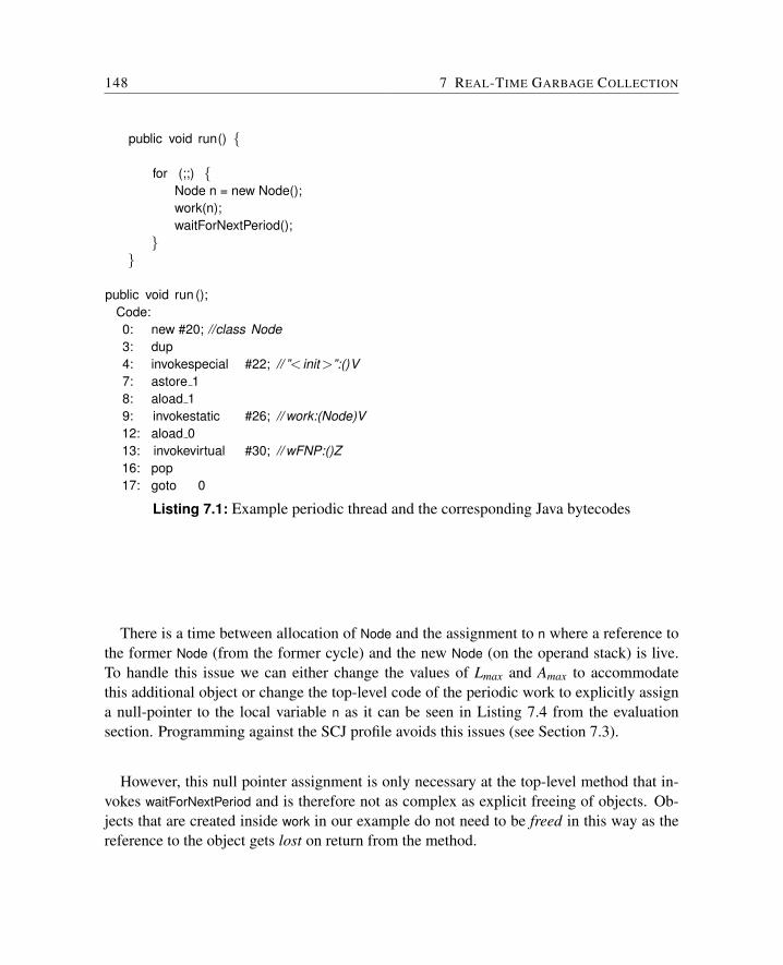
148 7 REAL-TIME GARBAGE COLLECTION
public void run() {
for (;;) {Node n = new Node();work(n);waitForNextPeriod();
}}
public void run ();Code:0: new #20; //class Node3: dup4: invokespecial #22; // ”< init >”:()V7: astore 18: aload 19: invokestatic #26; // work:(Node)V12: aload 013: invokevirtual #30; // wFNP:()Z16: pop17: goto 0
Listing 7.1: Example periodic thread and the corresponding Java bytecodes
There is a time between allocation of Node and the assignment to n where a reference tothe former Node (from the former cycle) and the new Node (on the operand stack) is live.To handle this issue we can either change the values of Lmax and Amax to accommodatethis additional object or change the top-level code of the periodic work to explicitly assigna null-pointer to the local variable n as it can be seen in Listing 7.4 from the evaluationsection. Programming against the SCJ profile avoids this issues (see Section 7.3).
However, this null pointer assignment is only necessary at the top-level method that in-vokes waitForNextPeriod and is therefore not as complex as explicit freeing of objects. Ob-jects that are created inside work in our example do not need to be freed in this way as thereference to the object gets lost on return from the method.
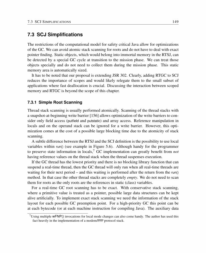
7.3 SCJ SIMPLIFICATIONS 149
7.3 SCJ Simplifications
The restrictions of the computational model for safety critical Java allow for optimizationsof the GC. We can avoid atomic stack scanning for roots and do not have to deal with exactpointer finding. Static objects, which would belong into immortal memory in the RTSJ, canbe detected by a special GC cycle at transition to the mission phase. We can treat thoseobjects specially and do not need to collect them during the mission phase. This staticmemory area is automatically sized.
It has to be noted that our proposal is extending JSR 302. Clearly, adding RTGC to SCJreduces the importance of scopes and would likely relegate them to the small subset ofapplications where fast deallocation is crucial. Discussing the interaction between scopedmemory and RTGC is beyond the scope of this chapter.
7.3.1 Simple Root Scanning
Thread stack scanning is usually performed atomically. Scanning of the thread stacks witha snapshot-at-beginning write barrier [156] allows optimization of the write barriers to con-sider only field access (putfield and putstatic) and array access. Reference manipulation inlocals and on the operand stack can be ignored for a write barrier. However, this opti-mization comes at the cost of a possible large blocking time due to the atomicity of stackscanning.
A subtle difference between the RTSJ and the SCJ definition is the possibility to use localvariables within run() (see example in Figure 5.6). Although handy for the programmerto preserve state information in locals,7 GC implementation can greatly benefit from nothaving reference values on the thread stack when the thread suspenses execution.
If the GC thread has the lowest priority and there is no blocking library function that cansuspend a real-time thread, then the GC thread will only run when all real-time threads arewaiting for their next period – and this waiting is performed after the return from the run()method. In that case the other thread stacks are completely empty. We do not need to scanthem for roots as the only roots are the references in static (class) variables.
For a real-time GC root scanning has to be exact. With conservative stack scanning,where a primitive value is treated as a pointer, possible large data structures can be keptalive artificially. To implement exact stack scanning we need the information of the stacklayout for each possible GC preemption point. For a high-priority GC this point can beat each bytecode (or at each machine instruction for compiling Java). The auxiliary data
7Using multiple wFNP() invocations for local mode changes can also come handy. The author has used thisfact heavily in the implementation of a modem/PPP protocol stack.
150 7 REAL-TIME GARBAGE COLLECTION
structure to capture the stack layout (and information which machine register will hold areference for compiled Java) can get quite large [92] or require additional effort to compute.
With a low-priority GC and the RTSJ model of periodic thread coding with wFNP() thenumber of GC preemption points is decreased dramatically. When the GC runs all threadswill be in wFNP(). Only the stack information for those places in the code have to beavailable. It is also assumed that wFNP() is not invoked very deep in the call hierarchy.Therefore, the stack high will be low and the resulting blocking time short.
As mentioned before, the SCJ style periodic thread model results in an empty stack atGC runtime. As a consequence we do not have to deal with exact stack scanning and needno additional information about the stack layout.
7.3.2 Static Memory
A SCJ copying collector will perform best when all live data is produced by periodic threadsand the maximum lifetime of a newly allocated object is one period. However, some datastructures allocated in the initialization phase stay alive for the whole application lifetime.In an RTSJ application this data would be allocated in immortal memory. With a real-timeGC there is no notion of immortal memory, instead we will use the term static memory.Without special treatment, a copying collector will move this data at each GC cycle. Fur-thermore, the memory demand for the collector increases by the amount of the static data.
As those static objects (mostly) live forever, we propose a solution similar to the im-mortal memory of the RTSJ. All data allocated during the initialization phase (where noapplication threads are scheduled) is considered potentially static. As part of the transitionto the mission phase a special collection cycle in a stop-the-world fashion is performed.Objects that are still alive after this cycle are assumed to live forever and make up the staticmemory area. The remaining memory is used for the garbage collected heap.
This static memory will still be scanned by the collector to find references into the heapbut it is not collected. The main differences between our static memory and the immortalmemory of the RTSJ are:
This static live data will still be scanned by the collector to find references into the heapbut it is not collected. The main differences between our immortal memory and the memoryareas of the RTSJ are:
• The choice of allocation context is implicit. There is no need to specify where anobject must be allocated. We do not have to state explicitly which data belongs to theapplication life-time data. This information is implicitly gathered by the start-missiontransition.
7.4 IMPLEMENTATION 151
• References from the static memory to the garbage collected heap are allowed contraryto the fact in the RTSJ that references to scoped memories, that have to be usedfor dynamic memory management without a GC, are not allowed from immortalmemory.
The second fact greatly simplifies communication between threads. For a typical produc-er/consumer configuration the container for the shared data is allocated in immortal memoryand the actual data in the garbage collected heap. With this immortal memory solution theactual Lmax only contains allocated memory from the periodic threads.
7.4 Implementation
The collector for JOP is an incremental collector [124, 138] based on the copy collectorby Cheney [32] and the incremental version by Baker [19]. To avoid the expensive readbarrier in Baker’s collector all object copies are performed concurrently by the collector.The collector is concurrent and resembles the collectors presented by Steele [142] and Di-jkstra et al. [38]. Therefore we call it the concurrent-copy collector.
The collector and the mutator are synchronized by two barriers. A Brooks-style [29]forwarding directs the access to the object either into tospace or fromspace. The forward-ing pointer is kept in a separate handle area as proposed in [89]. The separate handle areareduces the space overheads as only one pointer is needed for both object copies. Further-more, the indirection pointer does not need to be copied. The handle also contains otherobject related data, such as type information, and the mark list. The objects in the heap onlycontain the fields and no object header.
The second synchronization barrier is a snapshot-at-beginning write-barrier [156]. Asnapshot-at-beginning write-barrier synchronizes the mutator with the collector on a refer-ence store into a static field, an object field, or an array.
The whole collector, the new operation, and the write barriers are implemented in Java(with the help of native functions for direct memory access). The object copy operationis implemented in hardware and can be interrupted by mutator threads after each wordcopied [135]. The copy unit redirects the access to the object under copy, depending on theaccessed field, either to the original or the new version of the object.
Although we show the implementation on a Java processor, the GC is not JOP specificand can also be implemented on a conventional processor.
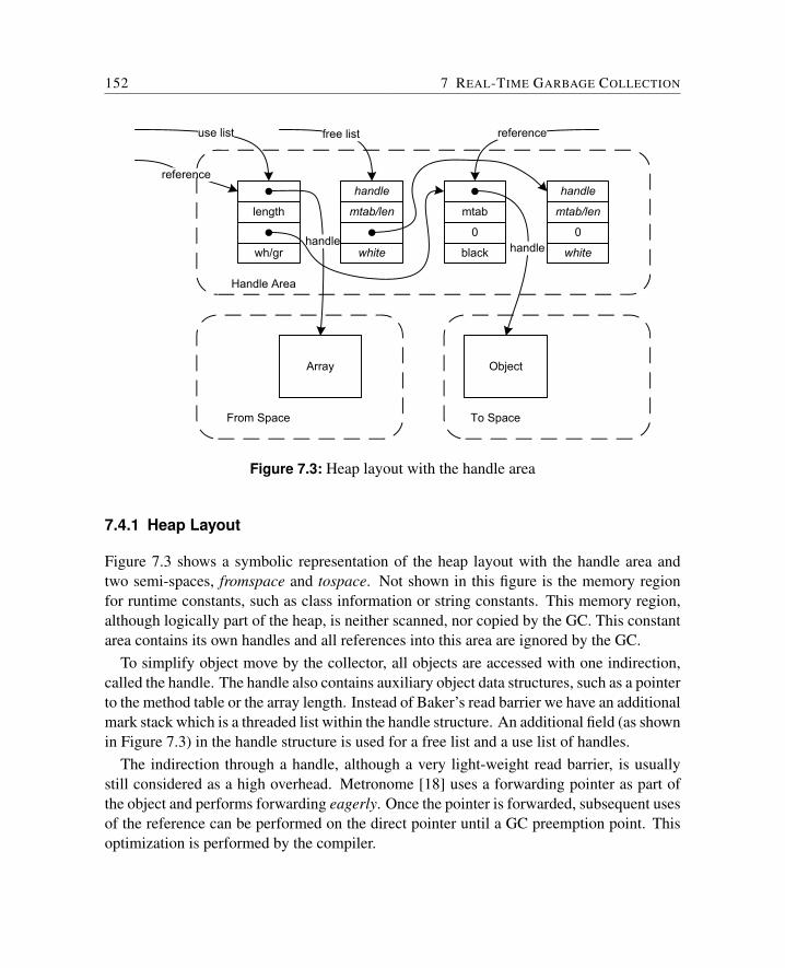
152 7 REAL-TIME GARBAGE COLLECTION
length
wh/gr
Array
handle
handle
mtab/len
white
0
mtab
black
handle
0
mtab/len
white
Object
reference
use list free list
handle
From Space To Space
Handle Area
reference
Figure 7.3: Heap layout with the handle area
7.4.1 Heap Layout
Figure 7.3 shows a symbolic representation of the heap layout with the handle area andtwo semi-spaces, fromspace and tospace. Not shown in this figure is the memory regionfor runtime constants, such as class information or string constants. This memory region,although logically part of the heap, is neither scanned, nor copied by the GC. This constantarea contains its own handles and all references into this area are ignored by the GC.
To simplify object move by the collector, all objects are accessed with one indirection,called the handle. The handle also contains auxiliary object data structures, such as a pointerto the method table or the array length. Instead of Baker’s read barrier we have an additionalmark stack which is a threaded list within the handle structure. An additional field (as shownin Figure 7.3) in the handle structure is used for a free list and a use list of handles.
The indirection through a handle, although a very light-weight read barrier, is usuallystill considered as a high overhead. Metronome [18] uses a forwarding pointer as part ofthe object and performs forwarding eagerly. Once the pointer is forwarded, subsequent usesof the reference can be performed on the direct pointer until a GC preemption point. Thisoptimization is performed by the compiler.
7.4 IMPLEMENTATION 153
JOP uses a hardware based optimization for this indirection [125]. The indirection isunconditionally performed in the memory access unit. Furthermore, null pointer checksand array bounds checks are done in parallel to this indirection.
There are two additional benefits from an explicit handle area instead of a forwardingpointer: (a) access to the method table or array size needs no indirection, and (b) the for-warding pointer and the auxiliary data structures do not need to be copied by the GC.
The fixed handle area is not subject to fragmentation as all handles have the same sizeand are recycled at a sweep phase with a simple free list. However, the reserved space hasto be sized (or the GC period adapted) for the maximum number of objects that are live orare floating garbage.
7.4.2 The Collector
The collector can operate in two modes: (1) as stop-the-world collector triggered on al-location when the heap is full, or (2) as concurrent real-time collector running in its ownthread.
The real-time collector is scheduled periodically at the lowest priority and within eachperiod it performs the following steps:
Flip An atomic flip exchanges the roles of tospace and fromspace.
Mark roots All static references are pushed onto the mark stack. Only a single push oper-ation needs to be atomic. As the thread stacks are empty we do not need an atomicscan of thread stacks.
Mark and copy An object is popped from the mark stack, all referenced objects, whichare still white, are pushed on the mark stack, the object is copied to tospace and thehandle pointer is updated.
Sweep handles All handles in the use list are checked if they still point into tospace (blackobjects) or can be added to the handle free list.
Clear fromspace At the end of the collector work the fromspace that contains only whiteobjects is initialized with zero. Objects allocated in that space (after the next flip) arealready initialized and allocation can be performed in constant time.
To reduce blocking time, a hardware unit performs copies of objects and arrays in an inter-ruptible fashion, and records the copy position on an interrupt. On an object or array accessthe hardware knows whether the access should go to the already copied part in the tospace
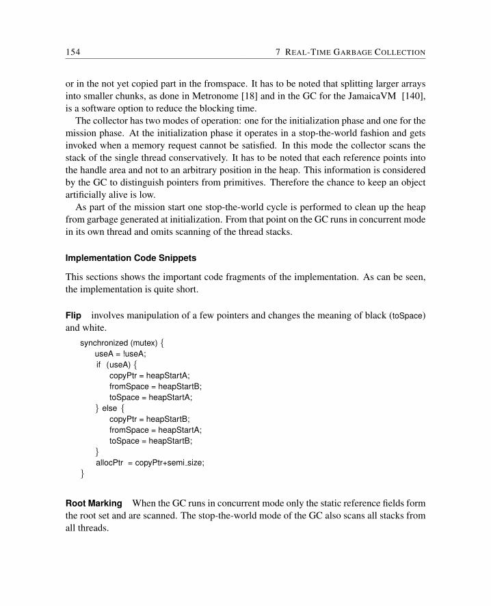
154 7 REAL-TIME GARBAGE COLLECTION
or in the not yet copied part in the fromspace. It has to be noted that splitting larger arraysinto smaller chunks, as done in Metronome [18] and in the GC for the JamaicaVM [140],is a software option to reduce the blocking time.
The collector has two modes of operation: one for the initialization phase and one for themission phase. At the initialization phase it operates in a stop-the-world fashion and getsinvoked when a memory request cannot be satisfied. In this mode the collector scans thestack of the single thread conservatively. It has to be noted that each reference points intothe handle area and not to an arbitrary position in the heap. This information is consideredby the GC to distinguish pointers from primitives. Therefore the chance to keep an objectartificially alive is low.
As part of the mission start one stop-the-world cycle is performed to clean up the heapfrom garbage generated at initialization. From that point on the GC runs in concurrent modein its own thread and omits scanning of the thread stacks.
Implementation Code Snippets
This sections shows the important code fragments of the implementation. As can be seen,the implementation is quite short.
Flip involves manipulation of a few pointers and changes the meaning of black (toSpace)and white.
synchronized (mutex) {useA = !useA;if (useA) {
copyPtr = heapStartA;fromSpace = heapStartB;toSpace = heapStartA;
} else {copyPtr = heapStartB;fromSpace = heapStartA;toSpace = heapStartB;
}allocPtr = copyPtr+semi size;
}
Root Marking When the GC runs in concurrent mode only the static reference fields formthe root set and are scanned. The stop-the-world mode of the GC also scans all stacks fromall threads.
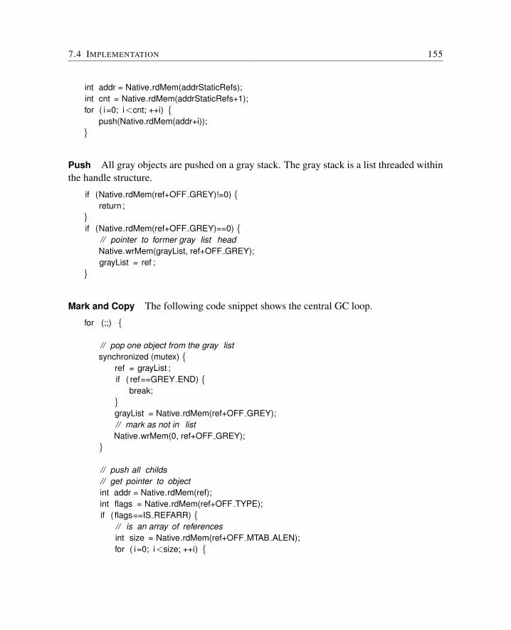
7.4 IMPLEMENTATION 155
int addr = Native.rdMem(addrStaticRefs);int cnt = Native.rdMem(addrStaticRefs+1);for ( i=0; i<cnt; ++i) {
push(Native.rdMem(addr+i));}
Push All gray objects are pushed on a gray stack. The gray stack is a list threaded withinthe handle structure.
if (Native.rdMem(ref+OFF GREY)!=0) {return ;
}if (Native.rdMem(ref+OFF GREY)==0) {
// pointer to former gray list headNative.wrMem(grayList, ref+OFF GREY);grayList = ref ;
}
Mark and Copy The following code snippet shows the central GC loop.
for (;;) {
// pop one object from the gray listsynchronized (mutex) {
ref = grayList ;if ( ref==GREY END) {
break;}grayList = Native.rdMem(ref+OFF GREY);// mark as not in listNative.wrMem(0, ref+OFF GREY);
}
// push all childs// get pointer to objectint addr = Native.rdMem(ref);int flags = Native.rdMem(ref+OFF TYPE);if ( flags==IS REFARR) {
// is an array of referencesint size = Native.rdMem(ref+OFF MTAB ALEN);for ( i=0; i<size; ++i) {
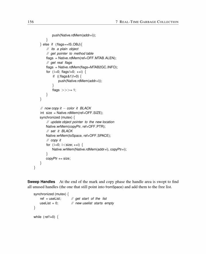
156 7 REAL-TIME GARBAGE COLLECTION
push(Native.rdMem(addr+i));}
} else if ( flags==IS OBJ){// its a plain object// get pointer to method tableflags = Native.rdMem(ref+OFF MTAB ALEN);// get real flagsflags = Native.rdMem(flags+MTAB2GC INFO);for ( i=0; flags !=0; ++i) {
if (( flags&1)!=0) {push(Native.rdMem(addr+i));
}flags >>>= 1;
}}
// now copy it − color it BLACKint size = Native.rdMem(ref+OFF SIZE);synchronized (mutex) {
// update object pointer to the new locationNative.wrMem(copyPtr, ref+OFF PTR);// set it BLACKNative.wrMem(toSpace, ref+OFF SPACE);// copy itfor ( i=0; i<size; ++i) {
Native.wrMem(Native.rdMem(addr+i), copyPtr+i);}copyPtr += size;
}}
Sweep Handles At the end of the mark and copy phase the handle area is swept to findall unused handles (the one that still point into fromSpace) and add them to the free list.
synchronized (mutex) {ref = useList; // get start of the listuseList = 0; // new uselist starts empty
}
while ( ref !=0) {
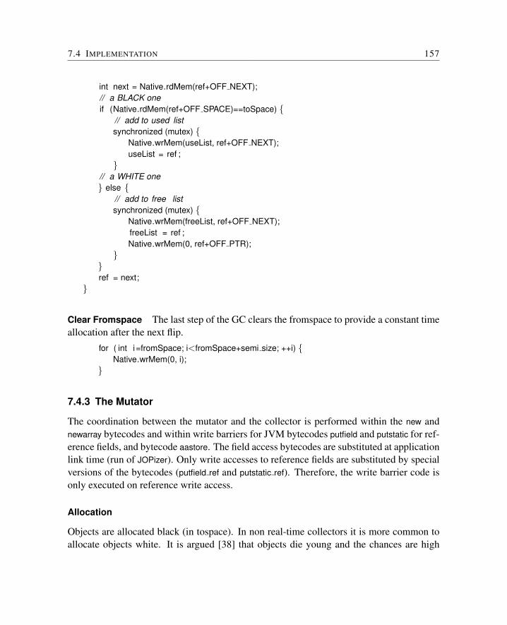
7.4 IMPLEMENTATION 157
int next = Native.rdMem(ref+OFF NEXT);// a BLACK oneif (Native.rdMem(ref+OFF SPACE)==toSpace) {
// add to used listsynchronized (mutex) {
Native.wrMem(useList, ref+OFF NEXT);useList = ref ;
}// a WHITE one} else {
// add to free listsynchronized (mutex) {
Native.wrMem(freeList, ref+OFF NEXT);freeList = ref ;Native.wrMem(0, ref+OFF PTR);
}}ref = next;
}
Clear Fromspace The last step of the GC clears the fromspace to provide a constant timeallocation after the next flip.
for ( int i=fromSpace; i<fromSpace+semi size; ++i) {Native.wrMem(0, i);
}
7.4.3 The Mutator
The coordination between the mutator and the collector is performed within the new andnewarray bytecodes and within write barriers for JVM bytecodes putfield and putstatic for ref-erence fields, and bytecode aastore. The field access bytecodes are substituted at applicationlink time (run of JOPizer). Only write accesses to reference fields are substituted by specialversions of the bytecodes (putfield ref and putstatic ref). Therefore, the write barrier code isonly executed on reference write access.
Allocation
Objects are allocated black (in tospace). In non real-time collectors it is more common toallocate objects white. It is argued [38] that objects die young and the chances are high
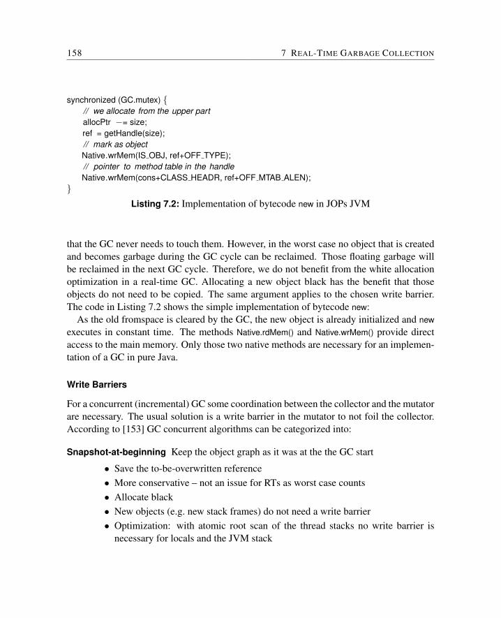
158 7 REAL-TIME GARBAGE COLLECTION
synchronized (GC.mutex) {// we allocate from the upper partallocPtr −= size;ref = getHandle(size);// mark as objectNative.wrMem(IS OBJ, ref+OFF TYPE);// pointer to method table in the handleNative.wrMem(cons+CLASS HEADR, ref+OFF MTAB ALEN);
}Listing 7.2: Implementation of bytecode new in JOPs JVM
that the GC never needs to touch them. However, in the worst case no object that is createdand becomes garbage during the GC cycle can be reclaimed. Those floating garbage willbe reclaimed in the next GC cycle. Therefore, we do not benefit from the white allocationoptimization in a real-time GC. Allocating a new object black has the benefit that thoseobjects do not need to be copied. The same argument applies to the chosen write barrier.The code in Listing 7.2 shows the simple implementation of bytecode new:
As the old fromspace is cleared by the GC, the new object is already initialized and newexecutes in constant time. The methods Native.rdMem() and Native.wrMem() provide directaccess to the main memory. Only those two native methods are necessary for an implemen-tation of a GC in pure Java.
Write Barriers
For a concurrent (incremental) GC some coordination between the collector and the mutatorare necessary. The usual solution is a write barrier in the mutator to not foil the collector.According to [153] GC concurrent algorithms can be categorized into:
Snapshot-at-beginning Keep the object graph as it was at the the GC start
• Save the to-be-overwritten reference• More conservative – not an issue for RTs as worst case counts• Allocate black• New objects (e.g. new stack frames) do not need a write barrier• Optimization: with atomic root scan of the thread stacks no write barrier is
necessary for locals and the JVM stack
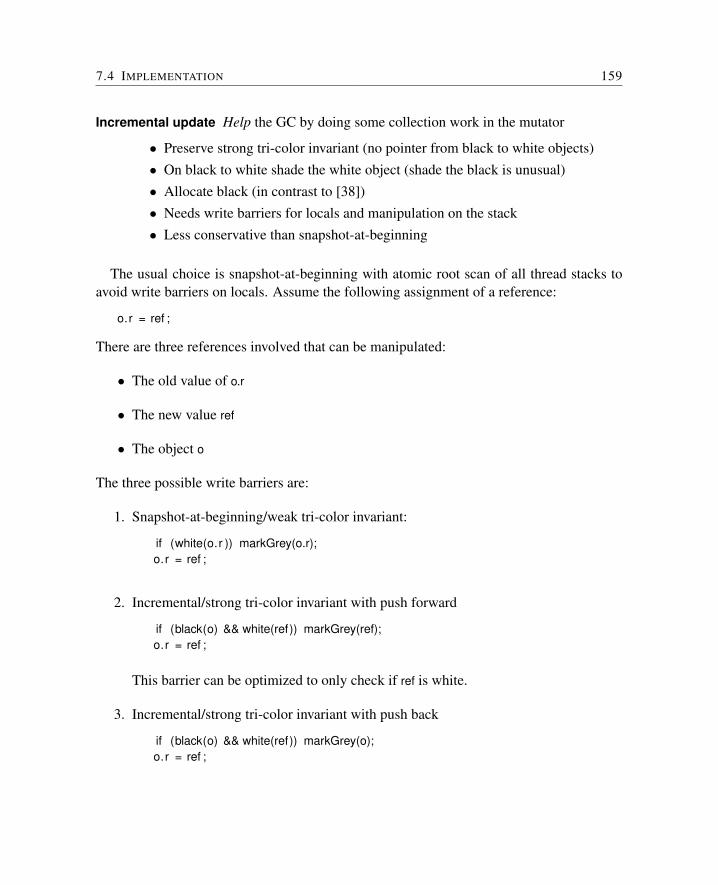
7.4 IMPLEMENTATION 159
Incremental update Help the GC by doing some collection work in the mutator
• Preserve strong tri-color invariant (no pointer from black to white objects)• On black to white shade the white object (shade the black is unusual)• Allocate black (in contrast to [38])• Needs write barriers for locals and manipulation on the stack• Less conservative than snapshot-at-beginning
The usual choice is snapshot-at-beginning with atomic root scan of all thread stacks toavoid write barriers on locals. Assume the following assignment of a reference:
o.r = ref ;
There are three references involved that can be manipulated:
• The old value of o.r
• The new value ref
• The object o
The three possible write barriers are:
1. Snapshot-at-beginning/weak tri-color invariant:
if (white(o.r )) markGrey(o.r);o.r = ref ;
2. Incremental/strong tri-color invariant with push forward
if (black(o) && white(ref)) markGrey(ref);o.r = ref ;
This barrier can be optimized to only check if ref is white.
3. Incremental/strong tri-color invariant with push back
if (black(o) && white(ref)) markGrey(o);o.r = ref ;
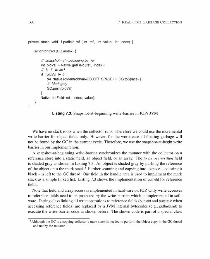
160 7 REAL-TIME GARBAGE COLLECTION
private static void f putfield ref ( int ref , int value, int index) {
synchronized (GC.mutex) {
// snapshot−at−beginning barrierint oldVal = Native.getField( ref , index);// Is it white?if (oldVal != 0
&& Native.rdMem(oldVal+GC.OFF SPACE) != GC.toSpace) {// Mark greyGC.push(oldVal)
}Native.putField( ref , index, value);
}}
Listing 7.3: Snapshot-at-beginning write-barrier in JOPs JVM
We have no stack roots when the collector runs. Therefore we could use the incrementalwrite barrier for object fields only. However, for the worst case all floating garbage willnot be found by the GC in the current cycle. Therefore, we use the snapshot-at-begin writebarrier in our implementation.
A snapshot-at-beginning write-barrier synchronizes the mutator with the collector on areference store into a static field, an object field, or an array. The to be overwritten fieldis shaded gray as shown in Listing 7.3. An object is shaded gray by pushing the referenceof the object onto the mark stack.8 Further scanning and copying into tospace – coloring itblack – is left to the GC thread. One field in the handle area is used to implement the markstack as a simple linked list. Listing 7.3 shows the implementation of putfield for referencefields.
Note that field and array access is implemented in hardware on JOP. Only write accessesto reference fields need to be protected by the write-barrier, which is implemented in soft-ware. During class linking all write operations to reference fields (putfield and putstatic whenaccessing reference fields) are replaced by a JVM internal bytecodes (e.g., putfield ref) toexecute the write-barrier code as shown before. The shown code is part of a special class
8Although the GC is a copying collector a mark stack is needed to perform the object copy in the GC threadand not by the mutator.
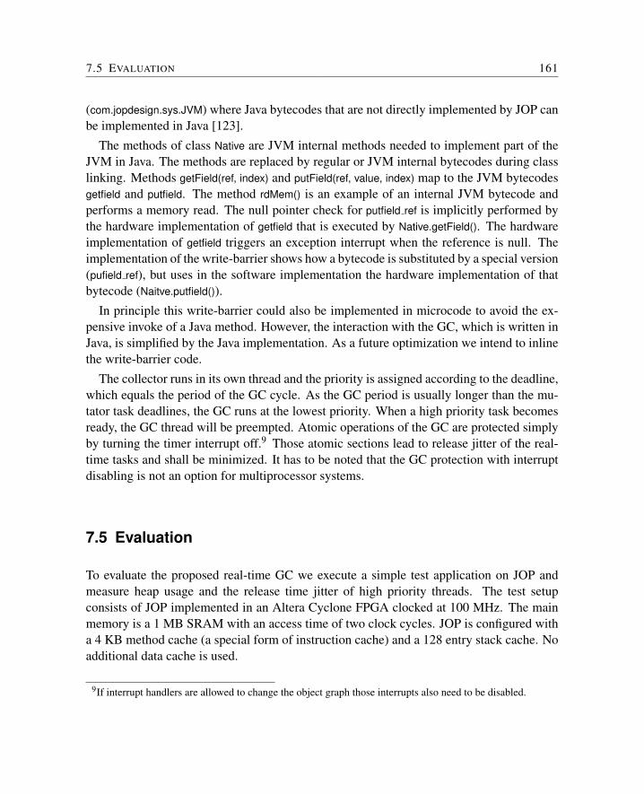
7.5 EVALUATION 161
(com.jopdesign.sys.JVM) where Java bytecodes that are not directly implemented by JOP canbe implemented in Java [123].
The methods of class Native are JVM internal methods needed to implement part of theJVM in Java. The methods are replaced by regular or JVM internal bytecodes during classlinking. Methods getField(ref, index) and putField(ref, value, index) map to the JVM bytecodesgetfield and putfield. The method rdMem() is an example of an internal JVM bytecode andperforms a memory read. The null pointer check for putfield ref is implicitly performed bythe hardware implementation of getfield that is executed by Native.getField(). The hardwareimplementation of getfield triggers an exception interrupt when the reference is null. Theimplementation of the write-barrier shows how a bytecode is substituted by a special version(pufield ref), but uses in the software implementation the hardware implementation of thatbytecode (Naitve.putfield()).
In principle this write-barrier could also be implemented in microcode to avoid the ex-pensive invoke of a Java method. However, the interaction with the GC, which is written inJava, is simplified by the Java implementation. As a future optimization we intend to inlinethe write-barrier code.
The collector runs in its own thread and the priority is assigned according to the deadline,which equals the period of the GC cycle. As the GC period is usually longer than the mu-tator task deadlines, the GC runs at the lowest priority. When a high priority task becomesready, the GC thread will be preempted. Atomic operations of the GC are protected simplyby turning the timer interrupt off.9 Those atomic sections lead to release jitter of the real-time tasks and shall be minimized. It has to be noted that the GC protection with interruptdisabling is not an option for multiprocessor systems.
7.5 Evaluation
To evaluate the proposed real-time GC we execute a simple test application on JOP andmeasure heap usage and the release time jitter of high priority threads. The test setupconsists of JOP implemented in an Altera Cyclone FPGA clocked at 100 MHz. The mainmemory is a 1 MB SRAM with an access time of two clock cycles. JOP is configured witha 4 KB method cache (a special form of instruction cache) and a 128 entry stack cache. Noadditional data cache is used.
9If interrupt handlers are allowed to change the object graph those interrupts also need to be disabled.
162 7 REAL-TIME GARBAGE COLLECTION
7.5.1 Scheduling Experiments
In this section we test an implementation of the concurrent-copy garbage collector on JOP.The tests are intended to get some confidence that the formulas for the collector periods arecorrect. Furthermore we visualize the actual heap usage of a running system.
The examples are synthetic benchmarks that emulate worst-case execution time (WCET)by executing a busy loop after allocation of the data. The WCET of the collector wasmeasured to be 10.4 ms when executing it with scheduling disabled during one collectioncycle for example 1 and 11.2 ms for example 2. We use 11 ms and 12 ms respectively asthe WCET of the collector for the following examples10.
Listing 7.4 shows our worker thread with the busy loop. The data is allocated at the startof the period and freed after the simulated execution. waitForNextPeriod blocks until the nextrelease time for the periodic thread.
For the busy loop to simulate real execution time, and not elapsed time, the constantMIN US has to be less than the time for two context switches, but larger than the executiontime of one iteration of the busy loop. In this case only cycles executed by the busy loop arecounted for the execution time and interruption due to a higher priority thread is not part ofthe execution time measurement.
In our example we use a concurrent-copy collector with a heap size (for both semi-spaces)of 100 KB. At startup the JVM allocates about 3.5 KB data. We incorporate11 these 3.5 KBas static live data Ls.
Independent Threads
The first example consists of two threads with the properties listed in Table 7.1. Ti is theperiod, Ci the WCET, and ai the maximum amount of memory allocated each period. Notethat the period for the collector thread is also listed in the table although it is a result of theworker thread properties and the heap size.
With the periods Ti and the memory consumption ai for the two worker threads we cal-
10It has to be noted that measuring execution time is not a safe method to estimate WCET values.11The suggested handling of static data to be moved to immortal memory at mission start is not yet imple-
mented.
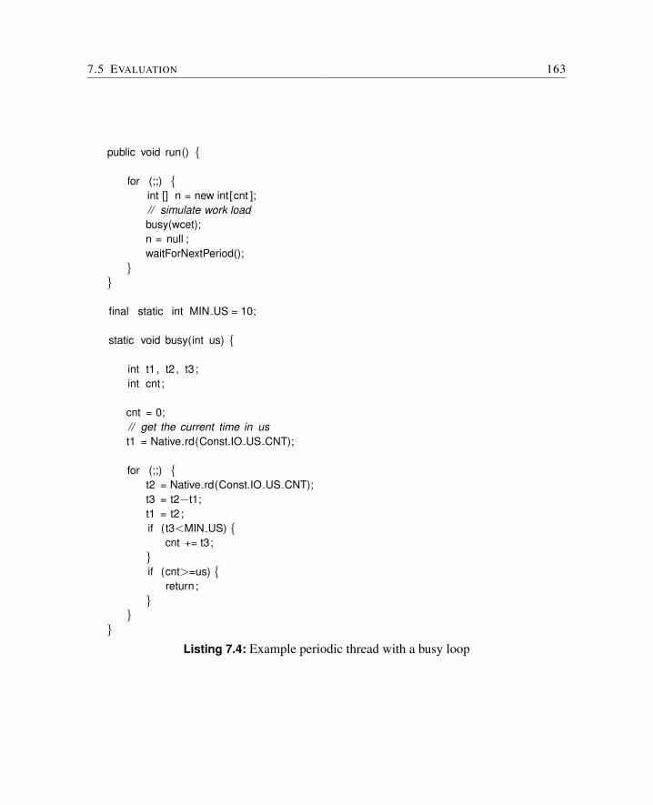
7.5 EVALUATION 163
public void run() {
for (;;) {int [] n = new int[cnt ];// simulate work loadbusy(wcet);n = null ;waitForNextPeriod();
}}
final static int MIN US = 10;
static void busy(int us) {
int t1 , t2 , t3 ;int cnt;
cnt = 0;// get the current time in ust1 = Native.rd(Const.IO US CNT);
for (;;) {t2 = Native.rd(Const.IO US CNT);t3 = t2−t1;t1 = t2 ;if ( t3<MIN US) {
cnt += t3;}if (cnt>=us) {
return ;}
}}
Listing 7.4: Example periodic thread with a busy loop
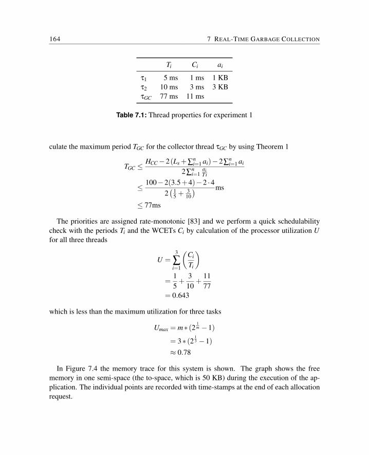
164 7 REAL-TIME GARBAGE COLLECTION
Ti Ci ai
τ1 5 ms 1 ms 1 KBτ2 10 ms 3 ms 3 KBτGC 77 ms 11 ms
Table 7.1: Thread properties for experiment 1
culate the maximum period TGC for the collector thread τGC by using Theorem 1
TGC ≤HCC−2(Ls +∑
ni=1 ai)−2∑
ni=1 ai
2∑ni=1
aiTi
≤ 100−2(3.5+4)−2 ·42( 1
5 + 310
) ms
≤ 77ms
The priorities are assigned rate-monotonic [83] and we perform a quick schedulabilitycheck with the periods Ti and the WCETs Ci by calculation of the processor utilization Ufor all three threads
U =3
∑i=1
(Ci
Ti
)=
15
+310
+1177
= 0.643
which is less than the maximum utilization for three tasks
Umax = m∗ (21m −1)
= 3∗ (213 −1)
≈ 0.78
In Figure 7.4 the memory trace for this system is shown. The graph shows the freememory in one semi-space (the to-space, which is 50 KB) during the execution of the ap-plication. The individual points are recorded with time-stamps at the end of each allocationrequest.

7.5 EVALUATION 165
30000
40000
50000
60000
ory
(Byt
e)
0
10000
20000
30000
40000
50000
60000
0 100 200 300 400 500 600
Free
Mem
ory
(Byt
e)
Time (ms)
Figure 7.4: Free memory in experiment 1
In the first milliseconds we see allocation requests that are part of the JVM startup (mostof it is static data). The change to the mission phase is delayed 100 ms and the first alloca-tion from a periodic thread is at 105 ms. The collector thread also starts at the same timeand the first semi-space flip can be seen at 110 ms (after one allocation from each workerthread). We see the 77 ms period of the collector in the jumps in the free memory graphafter the flip. The different memory requests of two times 1 KB from thread τ1 and onetime 3 KB from thread τ2 can be seen every 10 ms.
In this example the heap is used until it is almost full, but the application never runs outof memory and no thread misses a deadline. From the regular allocation pattern we also seethat this collector runs concurrently. With a stop-the-world collector we would notice gapsof 10 ms (the measured execution time of the collector) in the graph.
Producer/Consumer Threads
For the second experiment we split our thread τ1 to a producer thread τ1 and a consumerthread τ3 with a period of 30 ms. We assume after the split that the producer’s WCET ishalved to 500 us. The consumer thread is assumed to be more efficient when working onlager blocks of data than in the former example (C3=2 ms instead of 6*500 µs). The rest ofthe setting remains the same (the worker thread τ2). Table 7.2 shows the thread properties
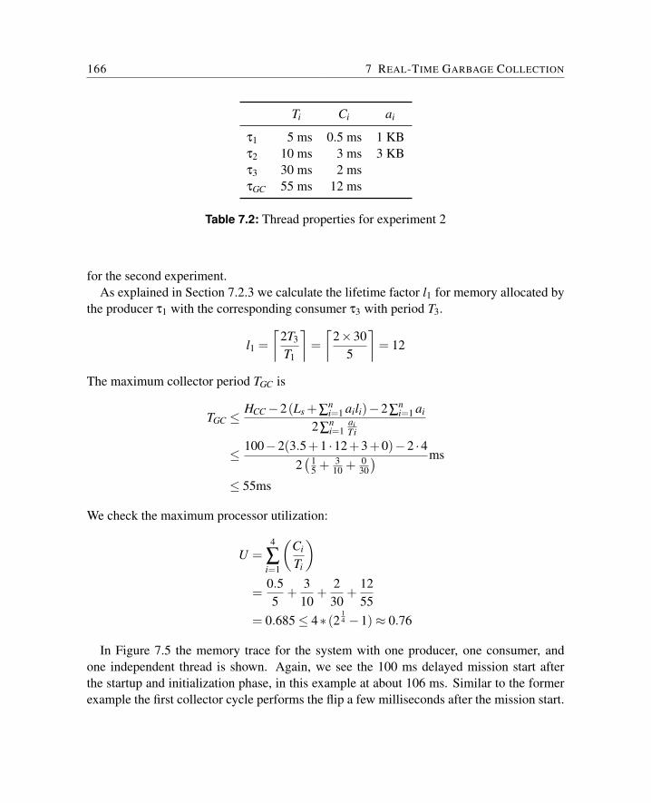
166 7 REAL-TIME GARBAGE COLLECTION
Ti Ci ai
τ1 5 ms 0.5 ms 1 KBτ2 10 ms 3 ms 3 KBτ3 30 ms 2 msτGC 55 ms 12 ms
Table 7.2: Thread properties for experiment 2
for the second experiment.As explained in Section 7.2.3 we calculate the lifetime factor l1 for memory allocated by
the producer τ1 with the corresponding consumer τ3 with period T3.
l1 =⌈
2T3
T1
⌉=⌈
2×305
⌉= 12
The maximum collector period TGC is
TGC ≤HCC−2(Ls +∑
ni=1 aili)−2∑
ni=1 ai
2∑ni=1
aiTi
≤ 100−2(3.5+1 ·12+3+0)−2 ·42(1
5 + 310 + 0
30
) ms
≤ 55ms
We check the maximum processor utilization:
U =4
∑i=1
(Ci
Ti
)=
0.55
+310
+230
+1255
= 0.685≤ 4∗ (214 −1)≈ 0.76
In Figure 7.5 the memory trace for the system with one producer, one consumer, andone independent thread is shown. Again, we see the 100 ms delayed mission start afterthe startup and initialization phase, in this example at about 106 ms. Similar to the formerexample the first collector cycle performs the flip a few milliseconds after the mission start.
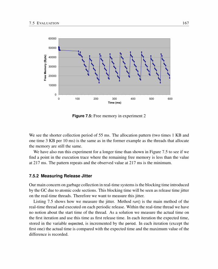
7.5 EVALUATION 167
30000
40000
50000
60000
ory
(Byt
e)
0
10000
20000
30000
40000
50000
60000
0 100 200 300 400 500 600
Free
Mem
ory
(Byt
e)
Time (ms)
Figure 7.5: Free memory in experiment 2
We see the shorter collection period of 55 ms. The allocation pattern (two times 1 KB andone time 3 KB per 10 ms) is the same as in the former example as the threads that allocatethe memory are still the same.
We have also run this experiment for a longer time than shown in Figure 7.5 to see if wefind a point in the execution trace where the remaining free memory is less than the valueat 217 ms. The pattern repeats and the observed value at 217 ms is the minimum.
7.5.2 Measuring Release Jitter
Our main concern on garbage collection in real-time systems is the blocking time introducedby the GC due to atomic code sections. This blocking time will be seen as release time jitteron the real-time threads. Therefore we want to measure this jitter.
Listing 7.5 shows how we measure the jitter. Method run() is the main method of thereal-time thread and executed on each periodic release. Within the real-time thread we haveno notion about the start time of the thread. As a solution we measure the actual time onthe first iteration and use this time as first release time. In each iteration the expected time,stored in the variable expected, is incremented by the period. In each iteration (except thefirst one) the actual time is compared with the expected time and the maximum value of thedifference is recorded.
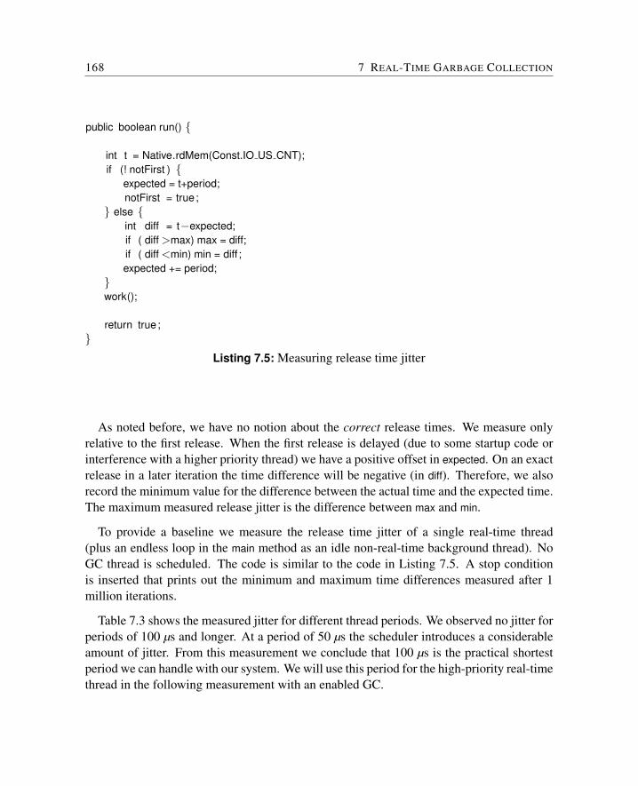
168 7 REAL-TIME GARBAGE COLLECTION
public boolean run() {
int t = Native.rdMem(Const.IO US CNT);if (! notFirst ) {
expected = t+period;notFirst = true;
} else {int diff = t−expected;if ( diff >max) max = diff;if ( diff <min) min = diff ;expected += period;
}work();
return true;}
Listing 7.5: Measuring release time jitter
As noted before, we have no notion about the correct release times. We measure onlyrelative to the first release. When the first release is delayed (due to some startup code orinterference with a higher priority thread) we have a positive offset in expected. On an exactrelease in a later iteration the time difference will be negative (in diff). Therefore, we alsorecord the minimum value for the difference between the actual time and the expected time.The maximum measured release jitter is the difference between max and min.
To provide a baseline we measure the release time jitter of a single real-time thread(plus an endless loop in the main method as an idle non-real-time background thread). NoGC thread is scheduled. The code is similar to the code in Listing 7.5. A stop conditionis inserted that prints out the minimum and maximum time differences measured after 1million iterations.
Table 7.3 shows the measured jitter for different thread periods. We observed no jitter forperiods of 100 µs and longer. At a period of 50 µs the scheduler introduces a considerableamount of jitter. From this measurement we conclude that 100 µs is the practical shortestperiod we can handle with our system. We will use this period for the high-priority real-timethread in the following measurement with an enabled GC.
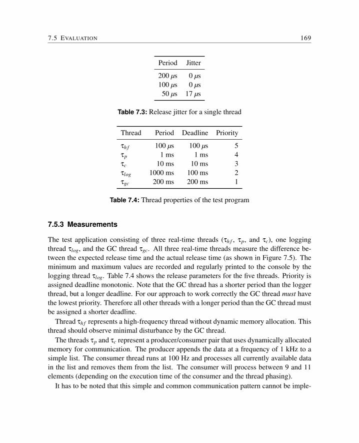
7.5 EVALUATION 169
Period Jitter
200 µs 0 µs100 µs 0 µs50 µs 17 µs
Table 7.3: Release jitter for a single thread
Thread Period Deadline Priority
τh f 100 µs 100 µs 5τp 1 ms 1 ms 4τc 10 ms 10 ms 3τlog 1000 ms 100 ms 2τgc 200 ms 200 ms 1
Table 7.4: Thread properties of the test program
7.5.3 Measurements
The test application consisting of three real-time threads (τh f , τp, and τc), one loggingthread τlog, and the GC thread τgc. All three real-time threads measure the difference be-tween the expected release time and the actual release time (as shown in Figure 7.5). Theminimum and maximum values are recorded and regularly printed to the console by thelogging thread τlog. Table 7.4 shows the release parameters for the five threads. Priority isassigned deadline monotonic. Note that the GC thread has a shorter period than the loggerthread, but a longer deadline. For our approach to work correctly the GC thread must havethe lowest priority. Therefore all other threads with a longer period than the GC thread mustbe assigned a shorter deadline.
Thread τh f represents a high-frequency thread without dynamic memory allocation. Thisthread should observe minimal disturbance by the GC thread.
The threads τp and τc represent a producer/consumer pair that uses dynamically allocatedmemory for communication. The producer appends the data at a frequency of 1 kHz to asimple list. The consumer thread runs at 100 Hz and processes all currently available datain the list and removes them from the list. The consumer will process between 9 and 11elements (depending on the execution time of the consumer and the thread phasing).
It has to be noted that this simple and common communication pattern cannot be imple-
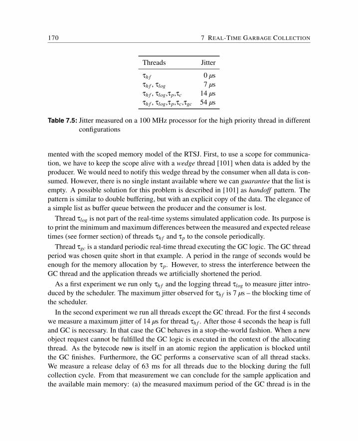
170 7 REAL-TIME GARBAGE COLLECTION
Threads Jitter
τh f 0 µsτh f , τlog 7 µsτh f , τlog,τp,τc 14 µsτh f , τlog,τp,τc,τgc 54 µs
Table 7.5: Jitter measured on a 100 MHz processor for the high priority thread in differentconfigurations
mented with the scoped memory model of the RTSJ. First, to use a scope for communica-tion, we have to keep the scope alive with a wedge thread [101] when data is added by theproducer. We would need to notify this wedge thread by the consumer when all data is con-sumed. However, there is no single instant available where we can guarantee that the list isempty. A possible solution for this problem is described in [101] as handoff pattern. Thepattern is similar to double buffering, but with an explicit copy of the data. The elegance ofa simple list as buffer queue between the producer and the consumer is lost.
Thread τlog is not part of the real-time systems simulated application code. Its purpose isto print the minimum and maximum differences between the measured and expected releasetimes (see former section) of threads τh f and τp to the console periodically.
Thread τgc is a standard periodic real-time thread executing the GC logic. The GC threadperiod was chosen quite short in that example. A period in the range of seconds would beenough for the memory allocation by τp. However, to stress the interference between theGC thread and the application threads we artificially shortened the period.
As a first experiment we run only τh f and the logging thread τlog to measure jitter intro-duced by the scheduler. The maximum jitter observed for τh f is 7 µs – the blocking time ofthe scheduler.
In the second experiment we run all threads except the GC thread. For the first 4 secondswe measure a maximum jitter of 14 µs for thread τh f . After those 4 seconds the heap is fulland GC is necessary. In that case the GC behaves in a stop-the-world fashion. When a newobject request cannot be fulfilled the GC logic is executed in the context of the allocatingthread. As the bytecode new is itself in an atomic region the application is blocked untilthe GC finishes. Furthermore, the GC performs a conservative scan of all thread stacks.We measure a release delay of 63 ms for all threads due to the blocking during the fullcollection cycle. From that measurement we can conclude for the sample application andthe available main memory: (a) the measured maximum period of the GC thread is in the
7.5 EVALUATION 171
range of 4 seconds; (b) the estimated execution time for one GC cycle is 63 ms. It has tobe noted that measurement is not a substitution for static timing analysis. Providing WCETestimates for a GC cycle is a challenge for future work.
In our final experiment we enabled all threads. The GC is scheduled periodically at200 ms as the lowest priority thread – the scenario we argue for. The GC logic is set intothe concurrent mode on mission start. In this mode the thread stacks are not scanned forroots. Furthermore when an allocation request cannot be fulfilled the application is stopped.This radical stop is intended for testing. In a more tolerant implementation either an out-of-memory exception can be thrown or the requesting thread has to be blocked, its threadstack scanned and released when the GC has finished its cycle.
We ran the experiment for several hours and recorded the maximum release jitter of thereal-time threads. For this test we used slightly different periods (prime numbers) to avoidthe regular phasing of the threads. The harmonic relation of the original periods can leadto too optimistic measurements. The applications never ran out of memory. The maximumjitter observed for the high priority task τh f was 54 µs. The maximum jitter for task τp was108 µs. This higher value on τp is expected as the execution interferes with the executionof the higher priority task τh f .
7.5.4 Discussion
With our measurements we have shown that quite short blocking times are achievable.Scheduling introduces a blocking time of about 7–14 µs and the GC adds another 40 µsresulting in a maximum jitter of the highest priority thread of 54 µs. In our first implemen-tation we performed the object copy in pure Java, resulting in blocking times around 200 µs.To speedup the copy we moved this function to microcode. However, the microcoded mem-cpy still needs 18 cycles per 32-bit word copy. Direct support in hardware can lead to acopy time of 4–5 clock cycles per word.
The maximum blocking time of 54 µs on a 100 MHz processor is less than blocking timesreported for other solutions.
Blocking time for Metronome (called pause times in the papers) is reported to be 6 ms[17] on a 500 MHz PowerPC at 50% CPU utilization. Those large blocking times are dueto the scheduling of the GC at the highest priority with a polling based yield within the GCthread. A fairer comparison is against the jitter of the pause time. In [16] the variation ofthe pause time is given between 500 µs and 2.4 ms on a 1 Ghz machine. It should be notedthat Metronome is a GC intended for mixed real-time systems whereas we aim only forhard real-time systems.
Robertz performed a similar measurement as we did for his thesis [114] with a time-
172 7 REAL-TIME GARBAGE COLLECTION
triggered GC on a 350 MHz PowerPC. He measured a maximum jitter of 20 µs (±10 µs)for a high priority task with a period of 500 µs.
It has to be noted that our experiment is a small one and we need more advanced real-time applications for the evaluation of real-time GC. The problem is that it is hard to findeven static based real-time application benchmarks (at least applications written for safetycritical Java). Running standard benchmarks that measure average case performance (e.g.,SPEC jvm98) is not an option to evaluate a real-time collector.
7.6 Analysis
To integrate GC into the WCET and scheduling analysis we need to know the worst-casememory consumption including the maximum lifetime of objects and the WCET of thecollector itself.
7.6.1 Worst Case Memory Consumption
Similar to the necessary WCET analysis of the tasks that make up the real-time system, aworst case memory allocation analysis of the tasks is necessary. For objects that are notshared between tasks this analysis can be performed by the same methods known from theWCET analysis. We have to find the worst-case program path that allocates the maximumamount of memory.
The analysis of memory consumption by objects that are shared between tasks for com-munication is more complex as an inter-task analysis is necessary.
7.6.2 WCET of the Collector
For the schedulability analysis the WCET of the collector has to be known. The collectorperforms following steps12:
1. Traverse the live object graph
2. Copy the live data
3. Initialize the free memory
12These steps can be distinct steps as in the mark-compact collector or interleaved as in the concurrent-copycollector.
7.7 SUMMARY 173
The execution time of the first step depends on the maximum amount of live data andthe number of references in each object. The second step depends on the size of the liveobjects. The last step depends on the size of the memory that gets freed during the collec-tion cycle. For a concurrent-copy collector this time is constant as a complete semi-spacegets initialized to zero. It has to be noted that this initialization could also be done at theallocation of the objects (as the LTMemory from the RTSJ implies). However, initializationin the collector is more efficient and the necessary time is easier to predict.
The maximum allocated memory and the type of the allocated objects determine the con-trol flow (the flow facts) of the collector. Therefore, this information has to be to incorporateinto WCET analysis of the collector thread.
7.7 Summary
In this chapter we have presented a real-time garbage collector in order to benefit from amore dynamic programming model for real-time applications. The collector is incrementaland scheduled as a normal real-time thread and, according to its deadline, assigned thelowest priority in the system. The restrictions from the SCJ programming model and thelow priority result in two advantages: (a) avoidance of stack root scanning and (b) shortblocking time of high priority threads. At 100 MHz we measured 40 µs maximum blockingtime introduced by the GC thread.
To guarantee that the applications will not run out of memory, the period of the collectorthread has to be short enough. We provided the maximum collector periods for a mark-compact collector type and a concurrent-copy collector. We have also shown how a longerlifetime due to object sharing between threads can be incorporated into the collector periodanalysis.
A critical operation for a concurrent, compacting GC is the atomic copy of large arrays.JOP has been extended by a copy unit that can be interrupted. This unit is integrated withthe memory access unit and redirects the access to either fromspace or tospace dependingon the array/field index and the value of the copy pointer.
7.8 Further Reading
Garbage collection was first introduced for list processing systems (LISP) in the 1960s.The first collectors were stop-the-world collectors that are called when a request for a newelement can not be fulfilled. The collector, starting from pointers known as the root set,scans the whole graph of reachable objects and marks these objects live. In a second phase
174 7 REAL-TIME GARBAGE COLLECTION
the collector sweeps the heap and adds unmarked objects to the free list. On the markedobjects, which are live, the mark is reset in preparation for the next cycle.
However, this simple sweep results in a fragmented heap which is an issue for objectsof different sizes. An extension, called mark-compact, moves the objects to compact theheap instead of the sweep. During this compaction all references to the moved objects areupdated to point to the new location.
Both collectors need a stack during the marking phase that can grow in the worst-case upto the number of live objects. Cheney [32] presents an elegant way how this mark stack canbe avoided. His GC is called copying-collector and divides the heap into two spaces: theto-space and the from-space. Objects are moved from one space to the other as part of thescan of the object graph.
However, all the described collectors are still stop-the-world collectors. The pause timeof up to seconds in large interactive LISP applications triggered the research on incrementalcollectors that distribute collection work more evenly [142, 38, 19]. These collectors weresometimes called real-time although they do not fulfill hard real-time properties that weneed today. A good overview of GC techniques can be found in [72] and in the GC surveyby Wilson [153].
Baker [19] extends Cheneys [32] copying collector for incremental GC. However, it usesan expensive read barrier that moves the object to the to-space as part of the mutator work.Baker proposes the Treadmill [20] to avoid copying. However, this collector works onlywith objects of equal size and still needs an expensive read barrier.
In [116] a garbage-collected memory module is suggested to provide a real-time collec-tor. A worst-case delay time of 1µs is claimed without giving the processor speed.
Metronome is a collector intended for soft real-time systems [18]. Non real-time appli-cations are used (SPECjvm98) in the experiments. They propose a collector with constantutilization to meet real-time requirements. However, utilization is not a real-time measureper se; it should be schedulability or response time instead. In contrast to our proposal theGC thread is scheduled at the highest priority in short periods. To ensure that, despite thehigh priority of the GC thread, mutator threads will be scheduled, the GC thread runs onlyfor a fraction of time within a time window. This fraction and the size of the time windowcan be adjusted for different work loads.
Although not mandated, all commercial and academic implementations of the RTSJ [140,26, 14, 10] and related real-time Java systems [6] also contain a real-time garbage collector.
In [95] two collectors based on [38] and [20] are implemented on a multithreaded micro-controller. Higuera suggests in [65] the use of hardware features from picoJava to speed upRTSJ memory region protection and garbage collection.
The work closest to our scheduling analysis is presented in [113]. The authors provide
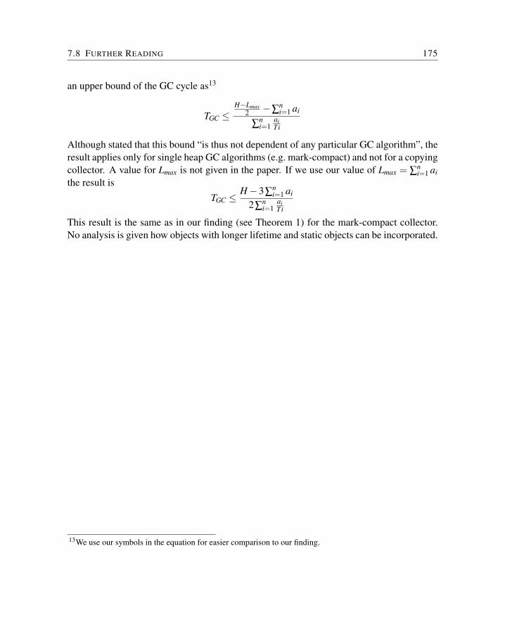
7.8 FURTHER READING 175
an upper bound of the GC cycle as13
TGC ≤H−Lmax
2 −∑ni=1 ai
∑ni=1
aiTi
Although stated that this bound “is thus not dependent of any particular GC algorithm”, theresult applies only for single heap GC algorithms (e.g. mark-compact) and not for a copyingcollector. A value for Lmax is not given in the paper. If we use our value of Lmax = ∑
ni=1 ai
the result isTGC ≤
H−3∑ni=1 ai
2∑ni=1
aiTi
This result is the same as in our finding (see Theorem 1) for the mark-compact collector.No analysis is given how objects with longer lifetime and static objects can be incorporated.
13We use our symbols in the equation for easier comparison to our finding.

8 Low-level I/O
The following section describes the low-level mechanism for I/O access and interrupts onJOP. As JOP is a Java processor no native functions (usually written in C) are available toaccess I/O directly or use C written interrupt handler. We need access to those low-levelfunctionality from Java for an embedded system. In the following a hardware abstractionlayer (HAL) in Java is proposed, where I/O devices are mapped to Java objects and interrupthandlers can be implemented in Java as Runnable. This section is based on [133] and [74].
8.1 Hardware Objects
Hardware objects map object fields to device registers. Therefore, field access with byte-codes putfield and getfield accesses device registers. With a correct class that represents adevice, access to it is safe – it is not possible to read or write to an arbitrary memory ad-dress. A memory area (e.g., a video frame buffer) represented by an array is protected byJava’s array bounds check. Representing I/O devices as first class objects has followingbenefits:
Object-oriented: An object representing a hardware device is the most natural integrationinto an OO language
Safe: The safety of Java is not compromised. We can access only those device registersthat are represented by the class definition
Efficient Device register access is performed by single bytecodes getfield and putfield. Weavoid expensive native calls.
8.1.1 An Example
Let us consider a simple I/O device, e.g. a parallel input/output (PIO) device – a commondevice in embedded systems for control applications. The PIO provides an interface be-tween I/O registers and I/O pins. The host captures data on the input pins with a registerread and drives data to the output pins with a register write. The example PIO contains two
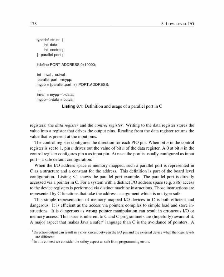
178 8 LOW-LEVEL I/O
typedef struct {int data;int control ;
} parallel port ;
#define PORT ADDRESS 0x10000;
int inval , outval ;parallel port ∗mypp;mypp = (parallel port ∗) PORT ADDRESS;...inval = mypp−>data;mypp−>data = outval;
Listing 8.1: Definition and usage of a parallel port in C
registers: the data register and the control register. Writing to the data register stores thevalue into a register that drives the output pins. Reading from the data register returns thevalue that is present at the input pins.
The control register configures the direction for each PIO pin. When bit n in the controlregister is set to 1, pin n drives out the value of bit n of the data register. A 0 at bit n in thecontrol register configures pin n as input pin. At reset the port is usually configured as inputport – a safe default configuration.1
When the I/O address space is memory mapped, such a parallel port is represented inC as a structure and a constant for the address. This definition is part of the board levelconfiguration. Listing 8.1 shows the parallel port example. The parallel port is directlyaccessed via a pointer in C. For a system with a distinct I/O address space (e.g. x86) accessto the device registers is performed via distinct machine instructions. Those instructions arerepresented by C functions that take the address as argument which is not type-safe.
This simple representation of memory mapped I/O devices in C is both efficient anddangerous. It is efficient as the access via pointers compiles to simple load and store in-structions. It is dangerous as wrong pointer manipulation can result in erroneous I/O ormemory access. This issue is inherent to C and C programmers are (hopefully) aware of it.A major aspect that makes Java a safer2 language than C is the avoidance of pointers. A
1Direction output can result in a short circuit between the I/O pin and the external device when the logic levelsare different.
2In this context we consider the safety aspect as safe from programming errors.
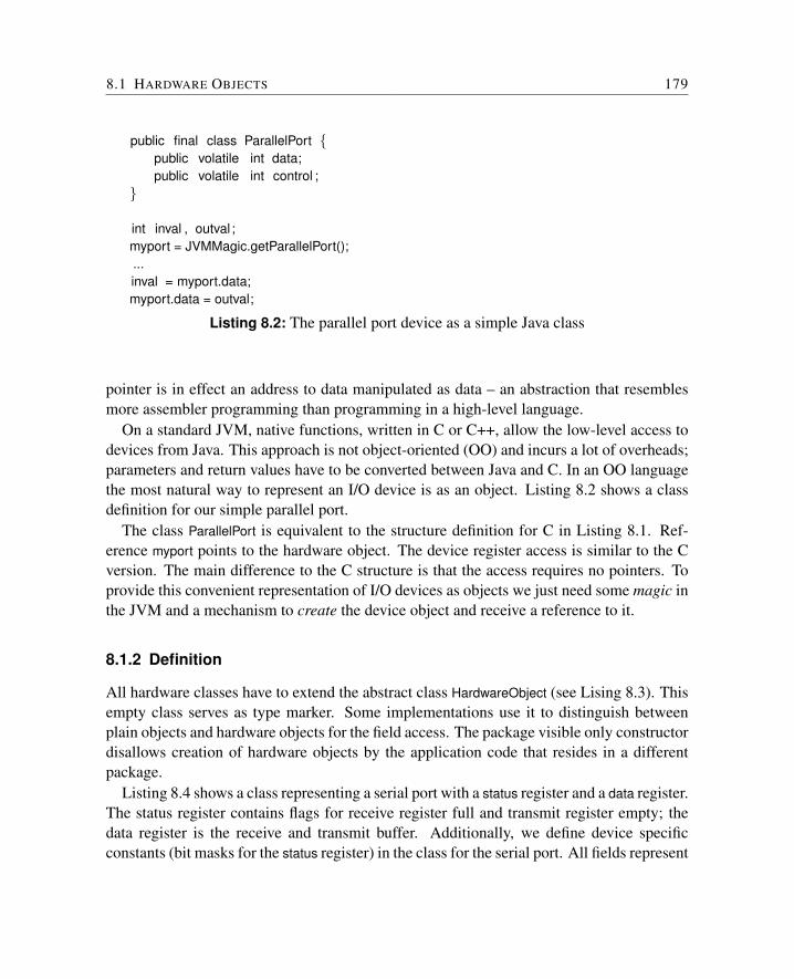
8.1 HARDWARE OBJECTS 179
public final class ParallelPort {public volatile int data;public volatile int control ;
}
int inval , outval ;myport = JVMMagic.getParallelPort();...inval = myport.data;myport.data = outval;
Listing 8.2: The parallel port device as a simple Java class
pointer is in effect an address to data manipulated as data – an abstraction that resemblesmore assembler programming than programming in a high-level language.
On a standard JVM, native functions, written in C or C++, allow the low-level access todevices from Java. This approach is not object-oriented (OO) and incurs a lot of overheads;parameters and return values have to be converted between Java and C. In an OO languagethe most natural way to represent an I/O device is as an object. Listing 8.2 shows a classdefinition for our simple parallel port.
The class ParallelPort is equivalent to the structure definition for C in Listing 8.1. Ref-erence myport points to the hardware object. The device register access is similar to the Cversion. The main difference to the C structure is that the access requires no pointers. Toprovide this convenient representation of I/O devices as objects we just need some magic inthe JVM and a mechanism to create the device object and receive a reference to it.
8.1.2 Definition
All hardware classes have to extend the abstract class HardwareObject (see Lising 8.3). Thisempty class serves as type marker. Some implementations use it to distinguish betweenplain objects and hardware objects for the field access. The package visible only constructordisallows creation of hardware objects by the application code that resides in a differentpackage.
Listing 8.4 shows a class representing a serial port with a status register and a data register.The status register contains flags for receive register full and transmit register empty; thedata register is the receive and transmit buffer. Additionally, we define device specificconstants (bit masks for the status register) in the class for the serial port. All fields represent
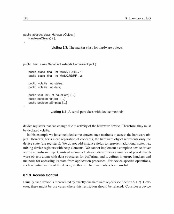
180 8 LOW-LEVEL I/O
public abstract class HardwareObject {HardwareObject() {};
}Listing 8.3: The marker class for hardware objects
public final class SerialPort extends HardwareObject {
public static final int MASK TDRE = 1;public static final int MASK RDRF = 2;
public volatile int status;public volatile int data;
public void init ( int baudRate) {...}public boolean rxFull () {...}public boolean txEmpty() {...}
}Listing 8.4: A serial port class with device methods
device registers that can change due to activity of the hardware device. Therefore, they mustbe declared volatile.
In this example we have included some convenience methods to access the hardware ob-ject. However, for a clear separation of concerns, the hardware object represents only thedevice state (the registers). We do not add instance fields to represent additional state, i.e.,mixing device registers with heap elements. We cannot implement a complete device driverwithin a hardware object; instead a complete device driver owns a number of private hard-ware objects along with data structures for buffering, and it defines interrupt handlers andmethods for accessing its state from application processes. For device specific operations,such as initialization of the device, methods in hardware objects are useful.
8.1.3 Access Control
Usually each device is represented by exactly one hardware object (see Section 8.1.7). How-ever, there might be use cases where this restriction should be relaxed. Consider a device
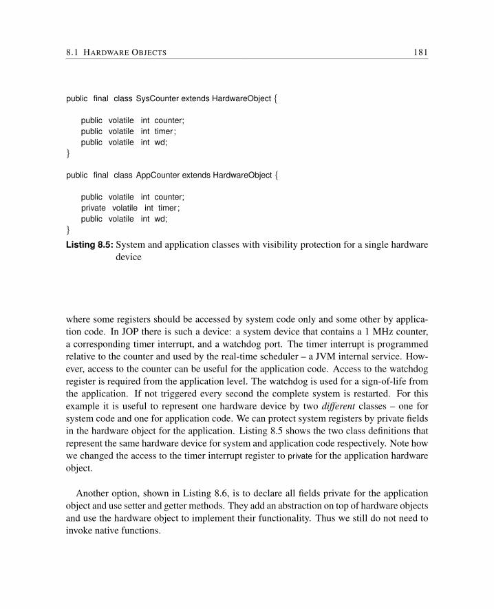
8.1 HARDWARE OBJECTS 181
public final class SysCounter extends HardwareObject {
public volatile int counter;public volatile int timer;public volatile int wd;
}
public final class AppCounter extends HardwareObject {
public volatile int counter;private volatile int timer;public volatile int wd;
}Listing 8.5: System and application classes with visibility protection for a single hardware
device
where some registers should be accessed by system code only and some other by applica-tion code. In JOP there is such a device: a system device that contains a 1 MHz counter,a corresponding timer interrupt, and a watchdog port. The timer interrupt is programmedrelative to the counter and used by the real-time scheduler – a JVM internal service. How-ever, access to the counter can be useful for the application code. Access to the watchdogregister is required from the application level. The watchdog is used for a sign-of-life fromthe application. If not triggered every second the complete system is restarted. For thisexample it is useful to represent one hardware device by two different classes – one forsystem code and one for application code. We can protect system registers by private fieldsin the hardware object for the application. Listing 8.5 shows the two class definitions thatrepresent the same hardware device for system and application code respectively. Note howwe changed the access to the timer interrupt register to private for the application hardwareobject.
Another option, shown in Listing 8.6, is to declare all fields private for the applicationobject and use setter and getter methods. They add an abstraction on top of hardware objectsand use the hardware object to implement their functionality. Thus we still do not need toinvoke native functions.
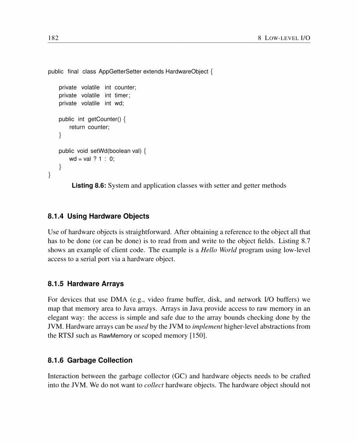
182 8 LOW-LEVEL I/O
public final class AppGetterSetter extends HardwareObject {
private volatile int counter;private volatile int timer;private volatile int wd;
public int getCounter() {return counter;
}
public void setWd(boolean val) {wd = val ? 1 : 0;
}}
Listing 8.6: System and application classes with setter and getter methods
8.1.4 Using Hardware Objects
Use of hardware objects is straightforward. After obtaining a reference to the object all thathas to be done (or can be done) is to read from and write to the object fields. Listing 8.7shows an example of client code. The example is a Hello World program using low-levelaccess to a serial port via a hardware object.
8.1.5 Hardware Arrays
For devices that use DMA (e.g., video frame buffer, disk, and network I/O buffers) wemap that memory area to Java arrays. Arrays in Java provide access to raw memory in anelegant way: the access is simple and safe due to the array bounds checking done by theJVM. Hardware arrays can be used by the JVM to implement higher-level abstractions fromthe RTSJ such as RawMemory or scoped memory [150].
8.1.6 Garbage Collection
Interaction between the garbage collector (GC) and hardware objects needs to be craftedinto the JVM. We do not want to collect hardware objects. The hardware object should not
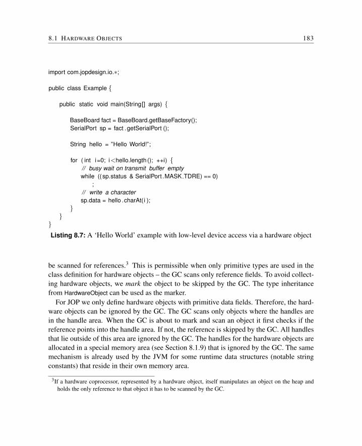
8.1 HARDWARE OBJECTS 183
import com.jopdesign.io.∗;
public class Example {
public static void main(String[] args) {
BaseBoard fact = BaseBoard.getBaseFactory();SerialPort sp = fact .getSerialPort ();
String hello = ”Hello World!”;
for ( int i=0; i<hello.length (); ++i) {// busy wait on transmit buffer emptywhile ((sp.status & SerialPort .MASK TDRE) == 0)
;// write a charactersp.data = hello .charAt(i );
}}
}Listing 8.7: A ‘Hello World’ example with low-level device access via a hardware object
be scanned for references.3 This is permissible when only primitive types are used in theclass definition for hardware objects – the GC scans only reference fields. To avoid collect-ing hardware objects, we mark the object to be skipped by the GC. The type inheritancefrom HardwareObject can be used as the marker.
For JOP we only define hardware objects with primitive data fields. Therefore, the hard-ware objects can be ignored by the GC. The GC scans only objects where the handles arein the handle area. When the GC is about to mark and scan an object it first checks if thereference points into the handle area. If not, the reference is skipped by the GC. All handlesthat lie outside of this area are ignored by the GC. The handles for the hardware objects areallocated in a special memory area (see Section 8.1.9) that is ignored by the GC. The samemechanism is already used by the JVM for some runtime data structures (notable stringconstants) that reside in their own memory area.
3If a hardware coprocessor, represented by a hardware object, itself manipulates an object on the heap andholds the only reference to that object it has to be scanned by the GC.
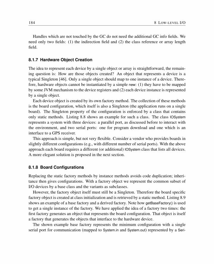
184 8 LOW-LEVEL I/O
Handles which are not touched by the GC do not need the additional GC info fields. Weneed only two fields: (1) the indirection field and (2) the class reference or array lengthfield.
8.1.7 Hardware Object Creation
The idea to represent each device by a single object or array is straightforward, the remain-ing question is: How are those objects created? An object that represents a device is atypical Singleton [46]. Only a single object should map to one instance of a device. There-fore, hardware objects cannot be instantiated by a simple new: (1) they have to be mappedby some JVM mechanism to the device registers and (2) each device instance is representedby a single object.
Each device object is created by its own factory method. The collection of these methodsis the board configuration, which itself is also a Singleton (the application runs on a singleboard). The Singleton property of the configuration is enforced by a class that containsonly static methods. Listing 8.8 shows an example for such a class. The class IOSystemrepresents a system with three devices: a parallel port, as discussed before to interact withthe environment, and two serial ports: one for program download and one which is aninterface to a GPS receiver.
This approach is simple, but not very flexible. Consider a vendor who provides boards inslightly different configurations (e.g., with different number of serial ports). With the aboveapproach each board requires a different (or additional) IOSystem class that lists all devices.A more elegant solution is proposed in the next section.
8.1.8 Board Configurations
Replacing the static factory methods by instance methods avoids code duplication; inheri-tance then gives configurations. With a factory object we represent the common subset ofI/O devices by a base class and the variants as subclasses.
However, the factory object itself must still be a Singleton. Therefore the board specificfactory object is created at class initialization and is retrieved by a static method. Listing 8.9shows an example of a base factory and a derived factory. Note how getBaseFactory() is usedto get a single instance of the factory. We have applied the idea of a factory two times: thefirst factory generates an object that represents the board configuration. That object is itselfa factory that generates the objects that interface to the hardware device.
The shown example base factory represents the minimum configuration with a singleserial port for communication (mapped to System.in and System.out) represented by a Seri-
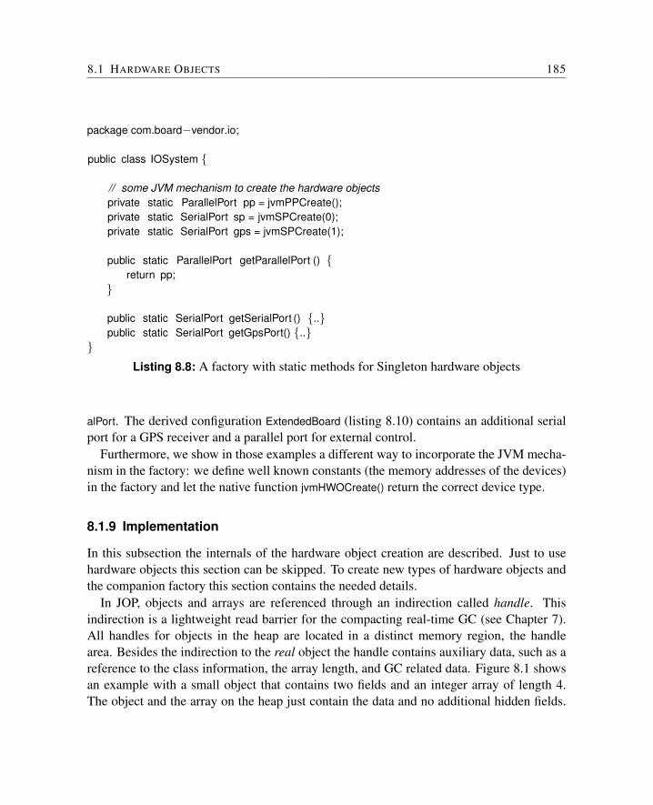
8.1 HARDWARE OBJECTS 185
package com.board−vendor.io;
public class IOSystem {
// some JVM mechanism to create the hardware objectsprivate static ParallelPort pp = jvmPPCreate();private static SerialPort sp = jvmSPCreate(0);private static SerialPort gps = jvmSPCreate(1);
public static ParallelPort getParallelPort () {return pp;
}
public static SerialPort getSerialPort () {..}public static SerialPort getGpsPort() {..}
}Listing 8.8: A factory with static methods for Singleton hardware objects
alPort. The derived configuration ExtendedBoard (listing 8.10) contains an additional serialport for a GPS receiver and a parallel port for external control.
Furthermore, we show in those examples a different way to incorporate the JVM mecha-nism in the factory: we define well known constants (the memory addresses of the devices)in the factory and let the native function jvmHWOCreate() return the correct device type.
8.1.9 Implementation
In this subsection the internals of the hardware object creation are described. Just to usehardware objects this section can be skipped. To create new types of hardware objects andthe companion factory this section contains the needed details.
In JOP, objects and arrays are referenced through an indirection called handle. Thisindirection is a lightweight read barrier for the compacting real-time GC (see Chapter 7).All handles for objects in the heap are located in a distinct memory region, the handlearea. Besides the indirection to the real object the handle contains auxiliary data, such as areference to the class information, the array length, and GC related data. Figure 8.1 showsan example with a small object that contains two fields and an integer array of length 4.The object and the array on the heap just contain the data and no additional hidden fields.
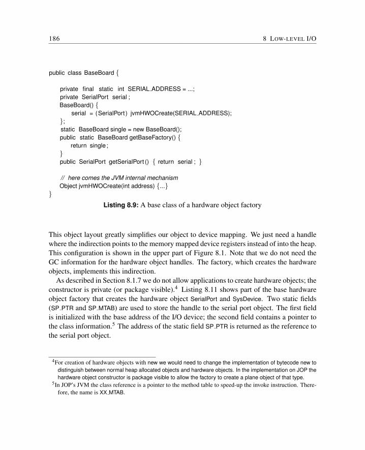
186 8 LOW-LEVEL I/O
public class BaseBoard {
private final static int SERIAL ADDRESS = ...;private SerialPort serial ;BaseBoard() {
serial = (SerialPort ) jvmHWOCreate(SERIAL ADDRESS);};static BaseBoard single = new BaseBoard();public static BaseBoard getBaseFactory() {
return single ;}public SerialPort getSerialPort () { return serial ; }
// here comes the JVM internal mechanismObject jvmHWOCreate(int address) {...}
}Listing 8.9: A base class of a hardware object factory
This object layout greatly simplifies our object to device mapping. We just need a handlewhere the indirection points to the memory mapped device registers instead of into the heap.This configuration is shown in the upper part of Figure 8.1. Note that we do not need theGC information for the hardware object handles. The factory, which creates the hardwareobjects, implements this indirection.
As described in Section 8.1.7 we do not allow applications to create hardware objects; theconstructor is private (or package visible).4 Listing 8.11 shows part of the base hardwareobject factory that creates the hardware object SerialPort and SysDevice. Two static fields(SP PTR and SP MTAB) are used to store the handle to the serial port object. The first fieldis initialized with the base address of the I/O device; the second field contains a pointer tothe class information.5 The address of the static field SP PTR is returned as the reference tothe serial port object.
4For creation of hardware objects with new we would need to change the implementation of bytecode new todistinguish between normal heap allocated objects and hardware objects. In the implementation on JOP thehardware object constructor is package visible to allow the factory to create a plane object of that type.
5In JOP’s JVM the class reference is a pointer to the method table to speed-up the invoke instruction. There-fore, the name is XX MTAB.
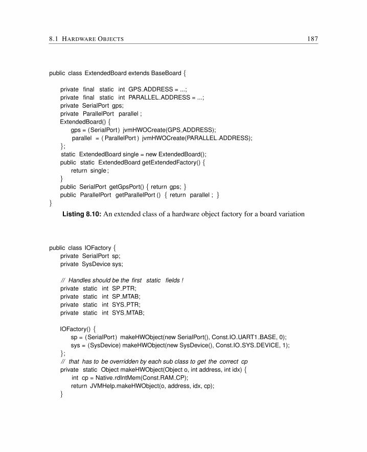
8.1 HARDWARE OBJECTS 187
public class ExtendedBoard extends BaseBoard {
private final static int GPS ADDRESS = ...;private final static int PARALLEL ADDRESS = ...;private SerialPort gps;private ParallelPort parallel ;ExtendedBoard() {
gps = (SerialPort ) jvmHWOCreate(GPS ADDRESS);parallel = ( ParallelPort ) jvmHWOCreate(PARALLEL ADDRESS);
};static ExtendedBoard single = new ExtendedBoard();public static ExtendedBoard getExtendedFactory() {
return single ;}public SerialPort getGpsPort() { return gps; }public ParallelPort getParallelPort () { return parallel ; }
}Listing 8.10: An extended class of a hardware object factory for a board variation
public class IOFactory {private SerialPort sp;private SysDevice sys;
// Handles should be the first static fields !private static int SP PTR;private static int SP MTAB;private static int SYS PTR;private static int SYS MTAB;
IOFactory() {sp = (SerialPort ) makeHWObject(new SerialPort(), Const.IO UART1 BASE, 0);sys = (SysDevice) makeHWObject(new SysDevice(), Const.IO SYS DEVICE, 1);
};// that has to be overridden by each sub class to get the correct cpprivate static Object makeHWObject(Object o, int address, int idx) {
int cp = Native.rdIntMem(Const.RAM CP);return JVMHelp.makeHWObject(o, address, idx, cp);
}
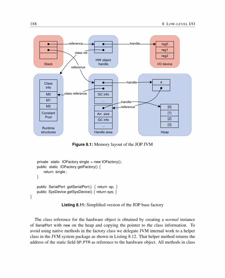
188 8 LOW-LEVEL I/O
I/O deviceHW object
handleStack
Handle area HeapRuntime
structures
GC info
...
handle
[0]
[2]
[1]
[3]GC info
Arr. size
...
a
handle
reference
reference
M0
Class info
M1
M2
Constant Pool
class reference
reference
class ref.
handle reg0
reg1
reg2
Figure 8.1: Memory layout of the JOP JVM
private static IOFactory single = new IOFactory();public static IOFactory getFactory() {
return single ;}
public SerialPort getSerialPort () { return sp; }public SysDevice getSysDevice() { return sys; }
}
Listing 8.11: Simplified version of the JOP base factory
The class reference for the hardware object is obtained by creating a normal instanceof SerialPort with new on the heap and copying the pointer to the class information. Toavoid using native methods in the factory class we delegate JVM internal work to a helperclass in the JVM system package as shown in Listing 8.12. That helper method returns theaddress of the static field SP PTR as reference to the hardware object. All methods in class
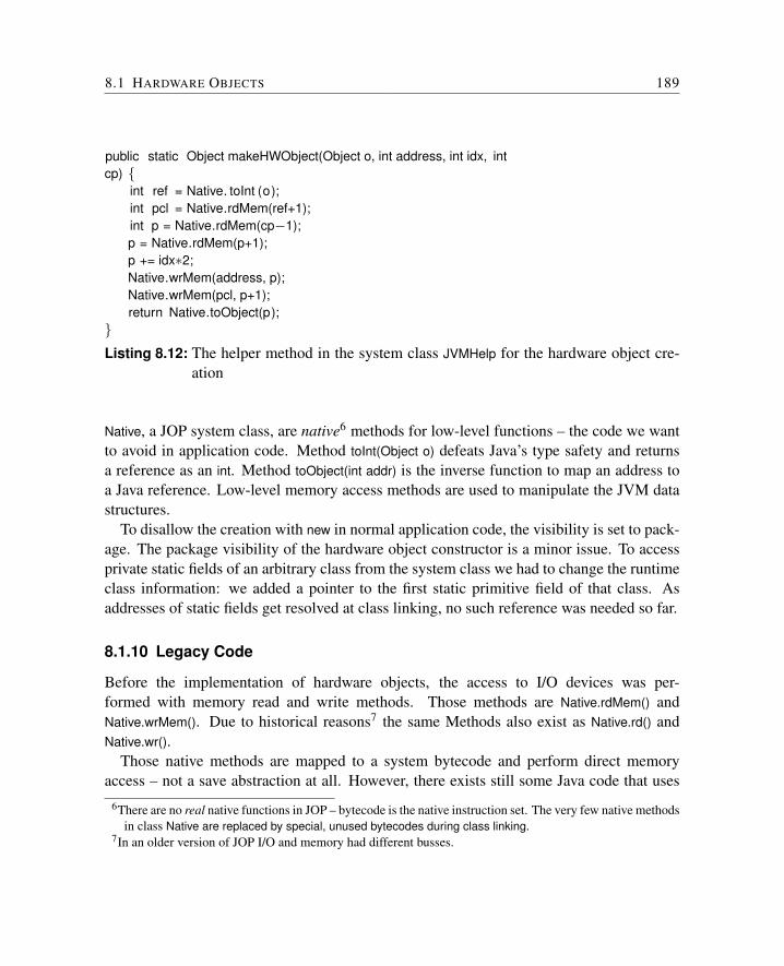
8.1 HARDWARE OBJECTS 189
public static Object makeHWObject(Object o, int address, int idx, intcp) {
int ref = Native. toInt (o);int pcl = Native.rdMem(ref+1);int p = Native.rdMem(cp−1);p = Native.rdMem(p+1);p += idx∗2;Native.wrMem(address, p);Native.wrMem(pcl, p+1);return Native.toObject(p);
}Listing 8.12: The helper method in the system class JVMHelp for the hardware object cre-
ation
Native, a JOP system class, are native6 methods for low-level functions – the code we wantto avoid in application code. Method toInt(Object o) defeats Java’s type safety and returnsa reference as an int. Method toObject(int addr) is the inverse function to map an address toa Java reference. Low-level memory access methods are used to manipulate the JVM datastructures.
To disallow the creation with new in normal application code, the visibility is set to pack-age. The package visibility of the hardware object constructor is a minor issue. To accessprivate static fields of an arbitrary class from the system class we had to change the runtimeclass information: we added a pointer to the first static primitive field of that class. Asaddresses of static fields get resolved at class linking, no such reference was needed so far.
8.1.10 Legacy Code
Before the implementation of hardware objects, the access to I/O devices was per-formed with memory read and write methods. Those methods are Native.rdMem() andNative.wrMem(). Due to historical reasons7 the same Methods also exist as Native.rd() andNative.wr().
Those native methods are mapped to a system bytecode and perform direct memoryaccess – not a save abstraction at all. However, there exists still some Java code that uses
6There are no real native functions in JOP – bytecode is the native instruction set. The very few native methodsin class Native are replaced by special, unused bytecodes during class linking.
7In an older version of JOP I/O and memory had different busses.
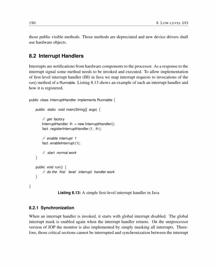
190 8 LOW-LEVEL I/O
those public visible methods. Those methods are depreciated and new device drivers shalluse hardware objects.
8.2 Interrupt Handlers
Interrupts are notifications from hardware components to the processor. As a response to theinterrupt signal some method needs to be invoked and executed. To allow implementationof first-level interrupt handler (IH) in Java we map interrupt requests to invocations of therun() method of a Runnable. Listing 8.13 shows an example of such an interrupt handler andhow it is registered.
public class InterruptHandler implements Runnable {
public static void main(String[] args) {
// get factoryInterruptHandler ih = new InterruptHandler();fact . registerInterruptHandler (1, ih );
// enable interrupt 1fact .enableInterrupt (1);
// start normal work}
public void run() {// do the first level interrupt handler work
}
}Listing 8.13: A simple first-level interrupt handler in Java
8.2.1 Synchronization
When an interrupt handler is invoked, it starts with global interrupt disabled. The globalinterrupt mask is enabled again when the interrupt handler returns. On the uniprocessorversion of JOP the monitor is also implemented by simply masking all interrupts. There-fore, those critical sections cannot be interrupted and synchronization between the interrupt
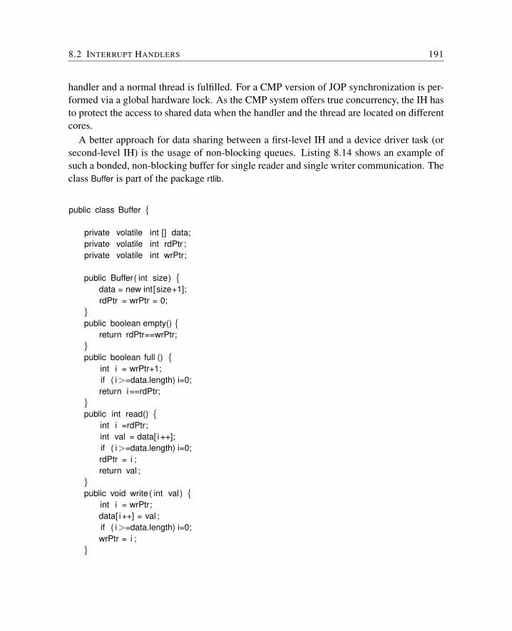
8.2 INTERRUPT HANDLERS 191
handler and a normal thread is fulfilled. For a CMP version of JOP synchronization is per-formed via a global hardware lock. As the CMP system offers true concurrency, the IH hasto protect the access to shared data when the handler and the thread are located on differentcores.
A better approach for data sharing between a first-level IH and a device driver task (orsecond-level IH) is the usage of non-blocking queues. Listing 8.14 shows an example ofsuch a bonded, non-blocking buffer for single reader and single writer communication. Theclass Buffer is part of the package rtlib.
public class Buffer {
private volatile int [] data;private volatile int rdPtr ;private volatile int wrPtr;
public Buffer( int size) {data = new int[size+1];rdPtr = wrPtr = 0;
}public boolean empty() {
return rdPtr==wrPtr;}public boolean full () {
int i = wrPtr+1;if ( i>=data.length) i=0;return i==rdPtr;
}public int read() {
int i =rdPtr;int val = data[ i ++];if ( i>=data.length) i=0;rdPtr = i ;return val ;
}public void write ( int val ) {
int i = wrPtr;data[ i++] = val ;if ( i>=data.length) i=0;wrPtr = i ;
}
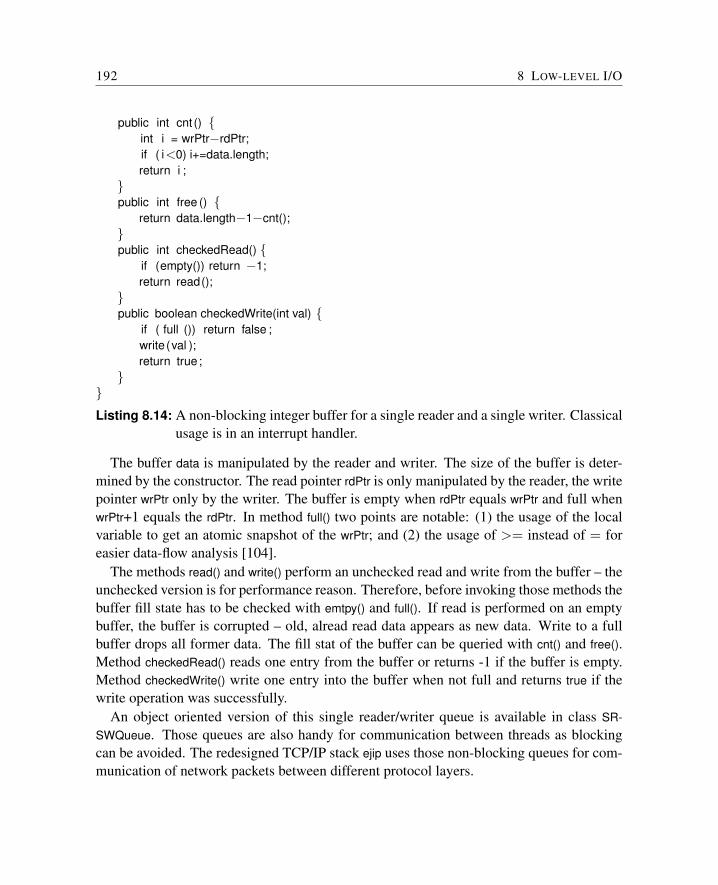
192 8 LOW-LEVEL I/O
public int cnt () {int i = wrPtr−rdPtr;if ( i<0) i+=data.length;return i ;
}public int free () {
return data.length−1−cnt();}public int checkedRead() {
if (empty()) return −1;return read();
}public boolean checkedWrite(int val) {
if ( full ()) return false ;write (val );return true;
}}
Listing 8.14: A non-blocking integer buffer for a single reader and a single writer. Classicalusage is in an interrupt handler.
The buffer data is manipulated by the reader and writer. The size of the buffer is deter-mined by the constructor. The read pointer rdPtr is only manipulated by the reader, the writepointer wrPtr only by the writer. The buffer is empty when rdPtr equals wrPtr and full whenwrPtr+1 equals the rdPtr. In method full() two points are notable: (1) the usage of the localvariable to get an atomic snapshot of the wrPtr; and (2) the usage of >= instead of = foreasier data-flow analysis [104].
The methods read() and write() perform an unchecked read and write from the buffer – theunchecked version is for performance reason. Therefore, before invoking those methods thebuffer fill state has to be checked with emtpy() and full(). If read is performed on an emptybuffer, the buffer is corrupted – old, alread read data appears as new data. Write to a fullbuffer drops all former data. The fill stat of the buffer can be queried with cnt() and free().Method checkedRead() reads one entry from the buffer or returns -1 if the buffer is empty.Method checkedWrite() write one entry into the buffer when not full and returns true if thewrite operation was successfully.
An object oriented version of this single reader/writer queue is available in class SR-SWQueue. Those queues are also handy for communication between threads as blockingcan be avoided. The redesigned TCP/IP stack ejip uses those non-blocking queues for com-munication of network packets between different protocol layers.
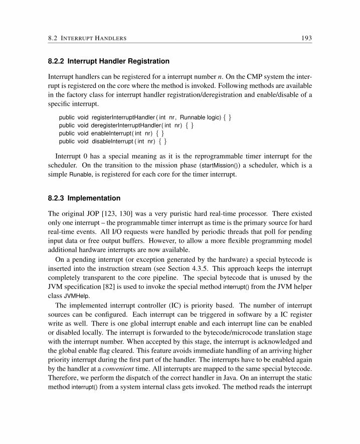
8.2 INTERRUPT HANDLERS 193
8.2.2 Interrupt Handler Registration
Interrupt handlers can be registered for a interrupt number n. On the CMP system the inter-rupt is registered on the core where the method is invoked. Following methods are availablein the factory class for interrupt handler registration/deregistration and enable/disable of aspecific interrupt.
public void registerInterruptHandler ( int nr, Runnable logic) { }public void deregisterInterruptHandler( int nr) { }public void enableInterrupt( int nr) { }public void disableInterrupt ( int nr) { }
Interrupt 0 has a special meaning as it is the reprogrammable timer interrupt for thescheduler. On the transition to the mission phase (startMission()) a scheduler, which is asimple Runable, is registered for each core for the timer interrupt.
8.2.3 Implementation
The original JOP [123, 130] was a very puristic hard real-time processor. There existedonly one interrupt – the programmable timer interrupt as time is the primary source for hardreal-time events. All I/O requests were handled by periodic threads that poll for pendinginput data or free output buffers. However, to allow a more flexible programming modeladditional hardware interrupts are now available.
On a pending interrupt (or exception generated by the hardware) a special bytecode isinserted into the instruction stream (see Section 4.3.5. This approach keeps the interruptcompletely transparent to the core pipeline. The special bytecode that is unused by theJVM specification [82] is used to invoke the special method interrupt() from the JVM helperclass JVMHelp.
The implemented interrupt controller (IC) is priority based. The number of interruptsources can be configured. Each interrupt can be triggered in software by a IC registerwrite as well. There is one global interrupt enable and each interrupt line can be enabledor disabled locally. The interrupt is forwarded to the bytecode/microcode translation stagewith the interrupt number. When accepted by this stage, the interrupt is acknowledged andthe global enable flag cleared. This feature avoids immediate handling of an arriving higherpriority interrupt during the first part of the handler. The interrupts have to be enabled againby the handler at a convenient time. All interrupts are mapped to the same special bytecode.Therefore, we perform the dispatch of the correct handler in Java. On an interrupt the staticmethod interrupt() from a system internal class gets invoked. The method reads the interrupt
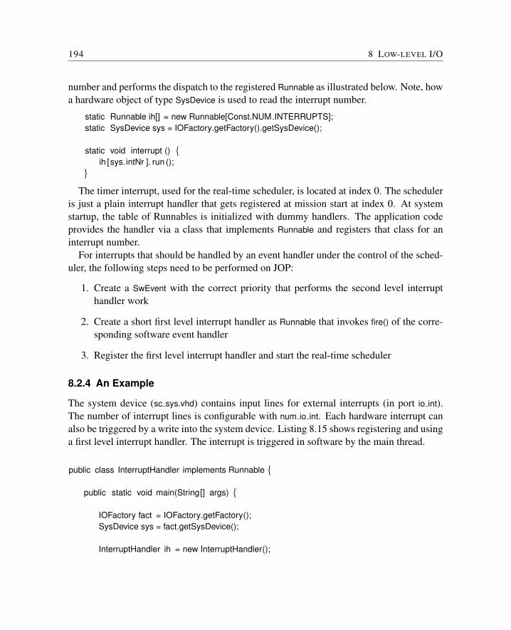
194 8 LOW-LEVEL I/O
number and performs the dispatch to the registered Runnable as illustrated below. Note, howa hardware object of type SysDevice is used to read the interrupt number.
static Runnable ih[] = new Runnable[Const.NUM INTERRUPTS];static SysDevice sys = IOFactory.getFactory().getSysDevice();
static void interrupt () {ih [sys.intNr ]. run ();
}
The timer interrupt, used for the real-time scheduler, is located at index 0. The scheduleris just a plain interrupt handler that gets registered at mission start at index 0. At systemstartup, the table of Runnables is initialized with dummy handlers. The application codeprovides the handler via a class that implements Runnable and registers that class for aninterrupt number.
For interrupts that should be handled by an event handler under the control of the sched-uler, the following steps need to be performed on JOP:
1. Create a SwEvent with the correct priority that performs the second level interrupthandler work
2. Create a short first level interrupt handler as Runnable that invokes fire() of the corre-sponding software event handler
3. Register the first level interrupt handler and start the real-time scheduler
8.2.4 An Example
The system device (sc sys.vhd) contains input lines for external interrupts (in port io int).The number of interrupt lines is configurable with num io int. Each hardware interrupt canalso be triggered by a write into the system device. Listing 8.15 shows registering and usinga first level interrupt handler. The interrupt is triggered in software by the main thread.
public class InterruptHandler implements Runnable {
public static void main(String[] args) {
IOFactory fact = IOFactory.getFactory();SysDevice sys = fact.getSysDevice();
InterruptHandler ih = new InterruptHandler();
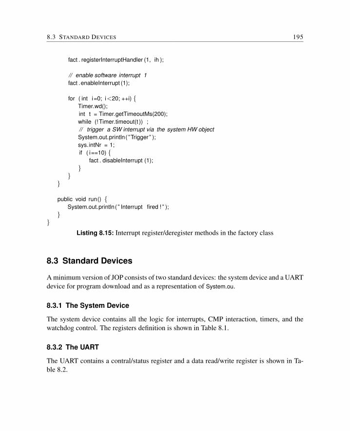
8.3 STANDARD DEVICES 195
fact . registerInterruptHandler (1, ih );
// enable software interrupt 1fact .enableInterrupt (1);
for ( int i=0; i<20; ++i) {Timer.wd();int t = Timer.getTimeoutMs(200);while (! Timer.timeout(t )) ;// trigger a SW interrupt via the system HW objectSystem.out.println( ”Trigger” );sys.intNr = 1;if ( i==10) {
fact . disableInterrupt (1);}
}}
public void run() {System.out.println( ” Interrupt fired ! ” );
}}
Listing 8.15: Interrupt register/deregister methods in the factory class
8.3 Standard Devices
A minimum version of JOP consists of two standard devices: the system device and a UARTdevice for program download and as a representation of System.ou.
8.3.1 The System Device
The system device contains all the logic for interrupts, CMP interaction, timers, and thewatchdog control. The registers definition is shown in Table 8.1.
8.3.2 The UART
The UART contains a contral/status register and a data read/write register is shown in Ta-ble 8.2.
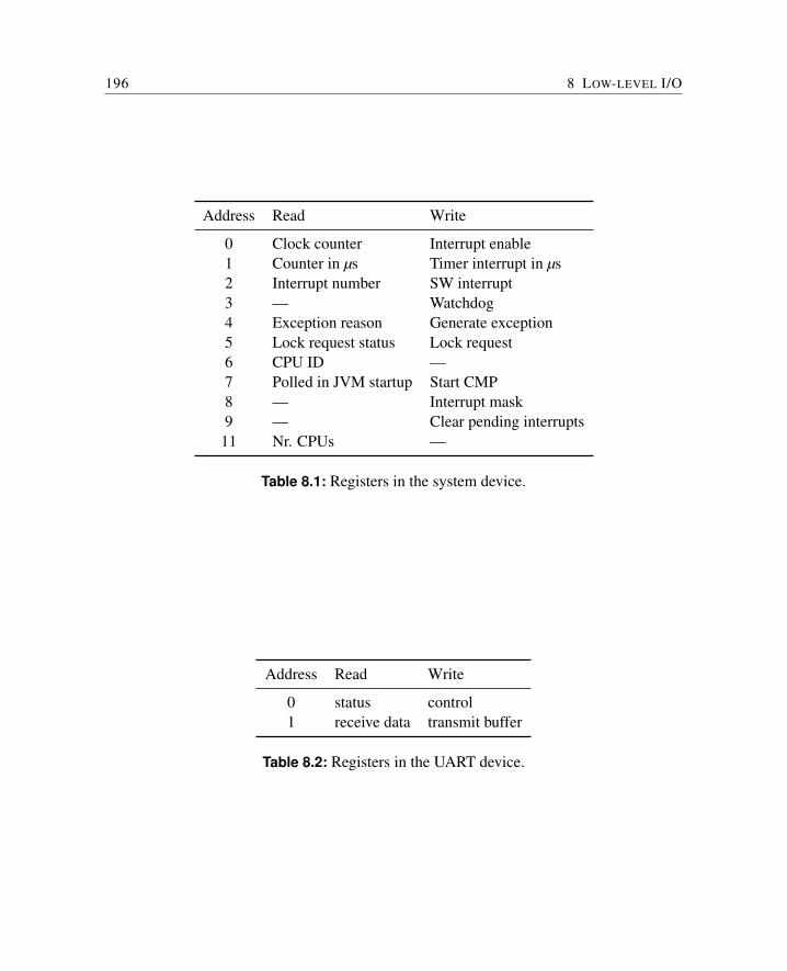
196 8 LOW-LEVEL I/O
Address Read Write
0 Clock counter Interrupt enable1 Counter in µs Timer interrupt in µs2 Interrupt number SW interrupt3 — Watchdog4 Exception reason Generate exception5 Lock request status Lock request6 CPU ID —7 Polled in JVM startup Start CMP8 — Interrupt mask9 — Clear pending interrupts11 Nr. CPUs —
Table 8.1: Registers in the system device.
Address Read Write
0 status control1 receive data transmit buffer
Table 8.2: Registers in the UART device.
9 The SimpCon Interconnect
SimpCon [127] is the main interconnection interface used for JOP. The I/O modules andthe main memory are connected via this standard. In the following chapter an introductionto SimpCon is presented.
The VHDL files in vhdl/scio are SimpCon I/O components (e.g. sc uart.vhd is a simpleUART) and SimpCon I/O configurations. The I/O configurations define the I/O devices andthe address mapping for a JOP system. All those configurations start with scio . The I/Ocomponents start with sc . Configuration scio min contains the minimal I/O components fora JOP system: the system module sc sys.vhd and a UART sc uart.vhd for program downloadand basic communication (System.in and System.out).
The system module sc sys.vhd contains the clock counter, the µs counter, timer inter-rupt, the SW interrupt, exception interrupts, the watchdog port, and the connection to themultiprocessor synchronization unit (cmpsync.vhd).
In directory vhdl/memory the memory controller mem sc.vhd is a SimpCon master that canbe connected to various SRAM memory controllers sc sram*.vhd. Other memory controller(e.g. the free Altera SDRAM interface) can be connected via SimpCon bridges to Avalon,Wishbone, and AHB slaves (available in vhdl/simpcon).
9.1 Introduction
The intention of the following SoC interconnect standard is to be simple and efficient withrespect to implementation resources and transaction latency.
SimpCon is a fully synchronous standard for on-chip interconnections. It is a point-to-point connection between a master and a slave. The master starts either a read or writetransaction. Master commands are single cycle to free the master to continue on internaloperations during an outstanding transaction. The slave has to register the address whenneeded for more than one cycle. The slave also registers the data on a read and providesit to the master for more than a single cycle. This property allows the master to delay theactual read if it is busy with internal operations.
The slave signals the end of the transaction through a novel ready counter to provide
198 9 THE SIMPCON INTERCONNECT
an early notification. This early notification simplifies the integration of peripherals intopipelined masters. Slaves can also provide several levels of pipelining. This feature isannounced by two static output ports (one for read and one write pipeline levels).
Off-chip connections (e.g. main memory) are device specific and need a slave to performthe translation. Peripheral interrupts are not covered by this specification.
9.1.1 Features
SimpCon provides following main features:
• Master/slave point-to-point connection
• Synchronous operation
• Read and write transactions
• Early pipeline release for the master
• Pipelined transactions
• Open-source specification
• Low implementation overheads
9.1.2 Basic Read Transaction
Figure 9.1 shows a basic read transaction for a slave with one cycle latency. In the firstcycle, the address phase, the rd signals the slave to start the read transaction. The address isregistered by the slave. During the following cycle, the read phase,1 the slave performs theread and registers the data. Due to the register in the slave, the data is available in the thirdcycle, the result phase. To simplify the master, rd data stays valid until the next read requestresponse. It is therefore possible for a master to issue a pre-fetch command early. When thepre-fetched data arrives too early it is still valid when the master actually wants to read it.Keeping the read data stable in the slave is mandatory.
1It has to be noted that the read phase can be longer for devices with a high latency. For simple on-chip I/Odevices the read phase can be omitted completely (0 cycles). In that case rdy cnt will be zero in the cyclefollowing the address phase.
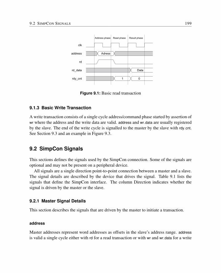
9.2 SIMPCON SIGNALS 199
Address phase Read phase Result phase
Adress
Data
clk
address
rd
rd_data
rdy_cnt 1 0
Figure 9.1: Basic read transaction
9.1.3 Basic Write Transaction
A write transaction consists of a single cycle address/command phase started by assertion ofwr where the address and the write data are valid. address and wr data are usually registeredby the slave. The end of the write cycle is signalled to the master by the slave with rdy cnt.See Section 9.3 and an example in Figure 9.3.
9.2 SimpCon Signals
This sections defines the signals used by the SimpCon connection. Some of the signals areoptional and may not be present on a peripheral device.
All signals are a single direction point-to-point connection between a master and a slave.The signal details are described by the device that drives the signal. Table 9.1 lists thesignals that define the SimpCon interface. The column Direction indicates whether thesignal is driven by the master or the slave.
9.2.1 Master Signal Details
This section describes the signals that are driven by the master to initiate a transaction.
address
Master addresses represent word addresses as offsets in the slave’s address range. addressis valid a single cycle either with rd for a read transaction or with wr and wr data for a write
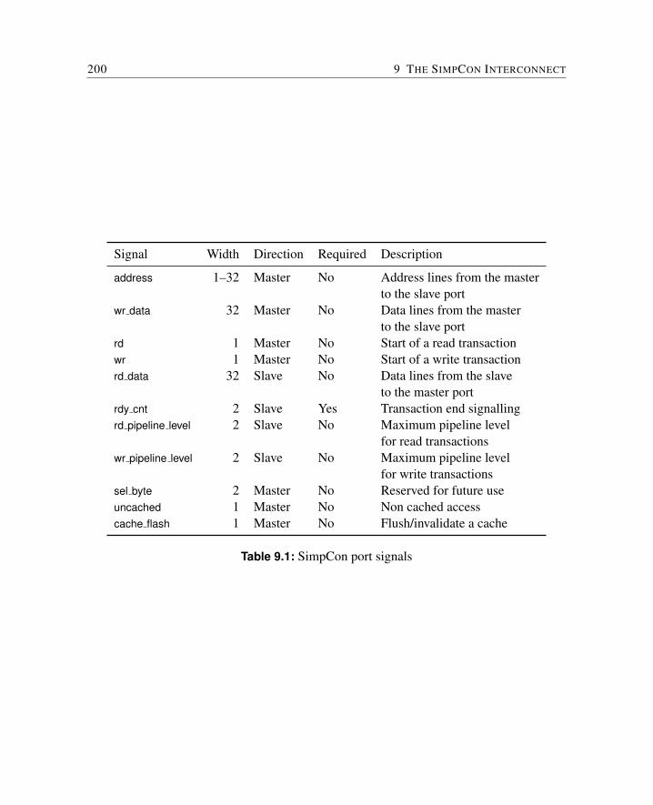
200 9 THE SIMPCON INTERCONNECT
Signal Width Direction Required Description
address 1–32 Master No Address lines from the masterto the slave port
wr data 32 Master No Data lines from the masterto the slave port
rd 1 Master No Start of a read transactionwr 1 Master No Start of a write transactionrd data 32 Slave No Data lines from the slave
to the master portrdy cnt 2 Slave Yes Transaction end signallingrd pipeline level 2 Slave No Maximum pipeline level
for read transactionswr pipeline level 2 Slave No Maximum pipeline level
for write transactionssel byte 2 Master No Reserved for future useuncached 1 Master No Non cached accesscache flash 1 Master No Flush/invalidate a cache
Table 9.1: SimpCon port signals
9.2 SIMPCON SIGNALS 201
transaction. The number of bits for address depends on the slave’s address range. For asingle port slave, address can be omitted.
wr data
The wr data signals carry the data for a write transaction. It is valid for a single cycletogether with address and wr. The signal is typically 32 bits wide. Slaves can ignore upperbits when the slave port is less than 32 bits.
rd
The rd signal is asserted for a single clock cycle to start a read transaction. address has tobe valid in the same cycle.
wr
The wr signal is asserted for a single clock cycle to start a write transaction. address andwr data have to be valid in the same cycle.
sel byte
The sel byte signal is reserved for future versions of the SimpCon specification to add indi-vidual byte enables.
uncached
The uncached signal is asserted for a single clock cycle during a read or write transactionto signal that a cache, connected in the SimpCon pipeline, shall not cache the read or writeaccess.
cache flash
The cache flash signal is asserted for a single clock cycle invalidates a cache connected inthe SimpCon pipeline.
9.2.2 Slave Signal Details
This section describes the signals that are driven by the slave as a response to transactionsinitiated by the master.
202 9 THE SIMPCON INTERCONNECT
rd data
The rd data signals carry the result of a read transaction. The data is valid when rdy cntreaches 0 and stays valid until a new read result is available. The signal is typically 32 bitswide. Slaves that provide less than 32 bits should pad the upper bits with 0.
rdy cnt
The rdy cnt signal provides the number of cycles until the pending transaction will finish. A0 means that either read data is available or a write transaction has been finished. Values of1 and 2 mean the transaction will finish in at least 1 or 2 cycles. The maximum value is 3and means the transaction will finish in 3 or more cycles. Note that not all values have to beused in a transaction. Each monotonic sequence of rdy cnt values is legal.
rd pipeline level
The static rd pipeline level provides the master with the read pipeline level of the slave. Thesignal has to be constant to enable the synthesizer to optimize the pipeline level dependentstate machine in the master.
wr pipeline level
The static wr pipeline level provides the master with the write pipeline level of the slave. Thesignal has to be constant to enable the synthesizer to optimize the pipeline level dependentstate machine in the master.
9.3 Slave Acknowledge
Flow control between the slave and the master is usually done by a single signal in the formof wait or acknowledge. The ack signal, e.g. in the Wishbone specification, is set when thedata is available or the write operation has finished. However, for a pipelined master it canbe of interest to know it earlier when a transaction will finish.
For many slaves, e.g. an SRAM interface with fixed wait states, this information is avail-able inside the slave. In the SimpCon interface, this information is communicated to themaster through the two bit ready counter (rdy cnt). rdy cnt signals the number of cycles untilthe read data will be available or the write transaction will be finished. A value of 0 is equiv-alent to an ack signal and 1, 2, and 3 are equivalent to a wait request with the distinctionthat the master knows how long the wait request will last.
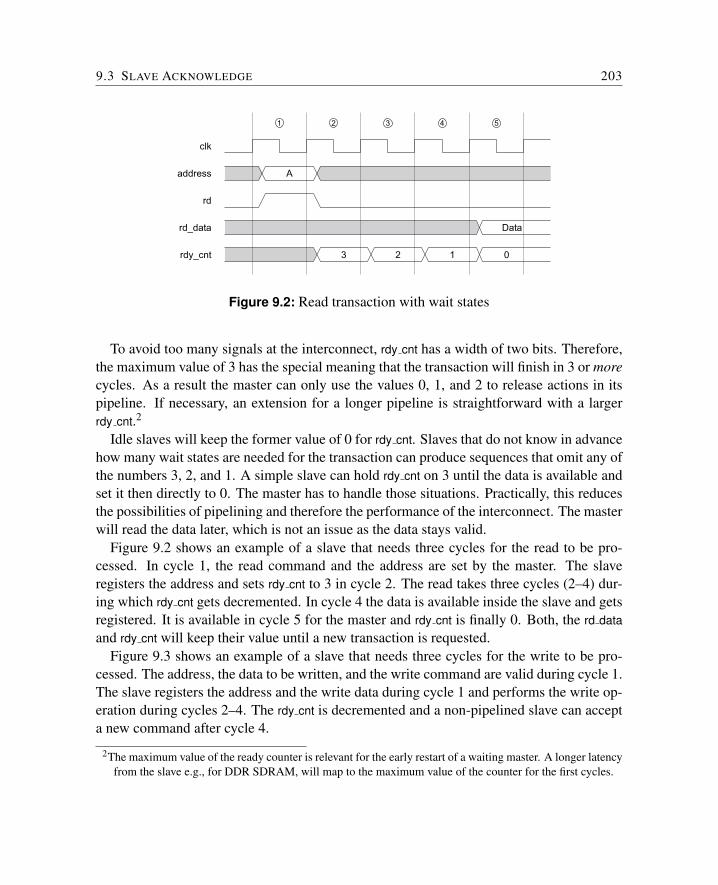
9.3 SLAVE ACKNOWLEDGE 203
A
Data
clk
address
rd
rd_data
rdy_cnt 3 2 1 0
1 2 3 4 5
Figure 9.2: Read transaction with wait states
To avoid too many signals at the interconnect, rdy cnt has a width of two bits. Therefore,the maximum value of 3 has the special meaning that the transaction will finish in 3 or morecycles. As a result the master can only use the values 0, 1, and 2 to release actions in itspipeline. If necessary, an extension for a longer pipeline is straightforward with a largerrdy cnt.2
Idle slaves will keep the former value of 0 for rdy cnt. Slaves that do not know in advancehow many wait states are needed for the transaction can produce sequences that omit any ofthe numbers 3, 2, and 1. A simple slave can hold rdy cnt on 3 until the data is available andset it then directly to 0. The master has to handle those situations. Practically, this reducesthe possibilities of pipelining and therefore the performance of the interconnect. The masterwill read the data later, which is not an issue as the data stays valid.
Figure 9.2 shows an example of a slave that needs three cycles for the read to be pro-cessed. In cycle 1, the read command and the address are set by the master. The slaveregisters the address and sets rdy cnt to 3 in cycle 2. The read takes three cycles (2–4) dur-ing which rdy cnt gets decremented. In cycle 4 the data is available inside the slave and getsregistered. It is available in cycle 5 for the master and rdy cnt is finally 0. Both, the rd dataand rdy cnt will keep their value until a new transaction is requested.
Figure 9.3 shows an example of a slave that needs three cycles for the write to be pro-cessed. The address, the data to be written, and the write command are valid during cycle 1.The slave registers the address and the write data during cycle 1 and performs the write op-eration during cycles 2–4. The rdy cnt is decremented and a non-pipelined slave can accepta new command after cycle 4.
2The maximum value of the ready counter is relevant for the early restart of a waiting master. A longer latencyfrom the slave e.g., for DDR SDRAM, will map to the maximum value of the counter for the first cycles.
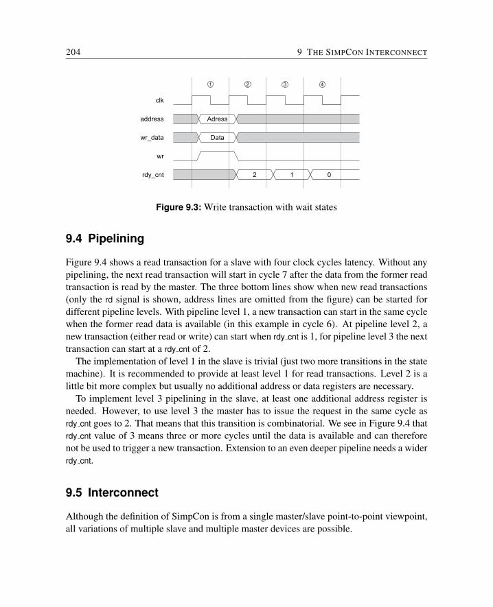
204 9 THE SIMPCON INTERCONNECT
Adress
clk
address
wr_data
wr
rdy_cnt 2 1 0
1 2 3 4
Data
Figure 9.3: Write transaction with wait states
9.4 Pipelining
Figure 9.4 shows a read transaction for a slave with four clock cycles latency. Without anypipelining, the next read transaction will start in cycle 7 after the data from the former readtransaction is read by the master. The three bottom lines show when new read transactions(only the rd signal is shown, address lines are omitted from the figure) can be started fordifferent pipeline levels. With pipeline level 1, a new transaction can start in the same cyclewhen the former read data is available (in this example in cycle 6). At pipeline level 2, anew transaction (either read or write) can start when rdy cnt is 1, for pipeline level 3 the nexttransaction can start at a rdy cnt of 2.
The implementation of level 1 in the slave is trivial (just two more transitions in the statemachine). It is recommended to provide at least level 1 for read transactions. Level 2 is alittle bit more complex but usually no additional address or data registers are necessary.
To implement level 3 pipelining in the slave, at least one additional address register isneeded. However, to use level 3 the master has to issue the request in the same cycle asrdy cnt goes to 2. That means that this transition is combinatorial. We see in Figure 9.4 thatrdy cnt value of 3 means three or more cycles until the data is available and can thereforenot be used to trigger a new transaction. Extension to an even deeper pipeline needs a widerrdy cnt.
9.5 Interconnect
Although the definition of SimpCon is from a single master/slave point-to-point viewpoint,all variations of multiple slave and multiple master devices are possible.
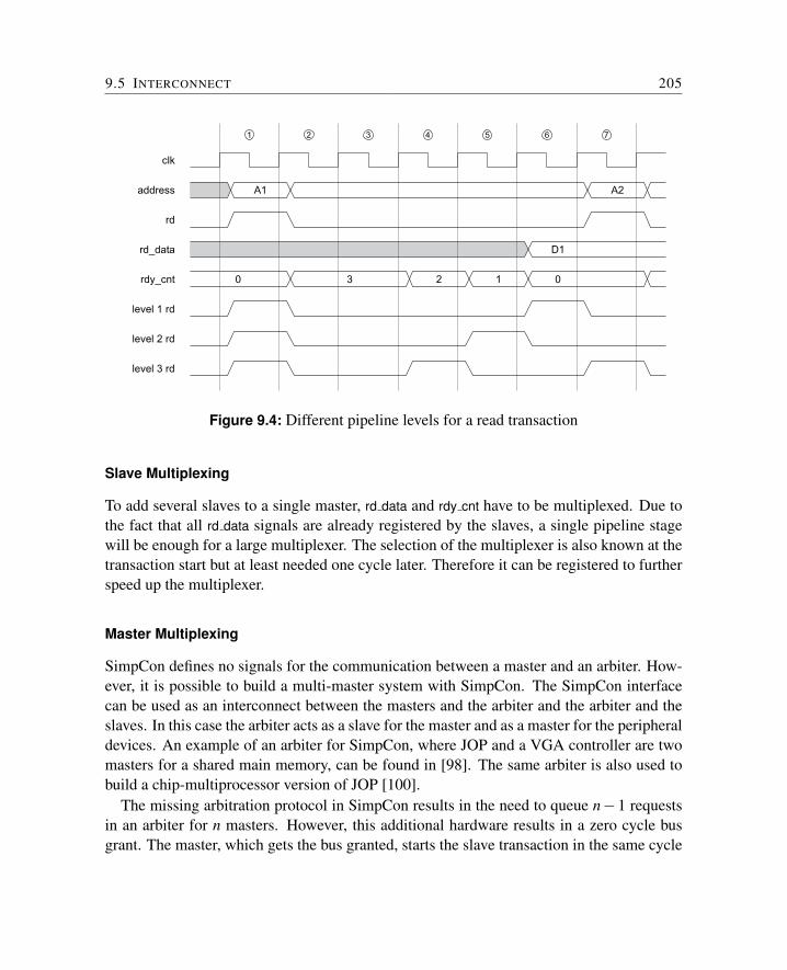
9.5 INTERCONNECT 205
A1
clk
address
rd_data
1 2 3 4 5 6 7
rd
rdy_cnt
level 1 rd
level 2 rd
level 3 rd
0 2 1 03
D1
A2
Figure 9.4: Different pipeline levels for a read transaction
Slave Multiplexing
To add several slaves to a single master, rd data and rdy cnt have to be multiplexed. Due tothe fact that all rd data signals are already registered by the slaves, a single pipeline stagewill be enough for a large multiplexer. The selection of the multiplexer is also known at thetransaction start but at least needed one cycle later. Therefore it can be registered to furtherspeed up the multiplexer.
Master Multiplexing
SimpCon defines no signals for the communication between a master and an arbiter. How-ever, it is possible to build a multi-master system with SimpCon. The SimpCon interfacecan be used as an interconnect between the masters and the arbiter and the arbiter and theslaves. In this case the arbiter acts as a slave for the master and as a master for the peripheraldevices. An example of an arbiter for SimpCon, where JOP and a VGA controller are twomasters for a shared main memory, can be found in [98]. The same arbiter is also used tobuild a chip-multiprocessor version of JOP [100].
The missing arbitration protocol in SimpCon results in the need to queue n−1 requestsin an arbiter for n masters. However, this additional hardware results in a zero cycle busgrant. The master, which gets the bus granted, starts the slave transaction in the same cycle
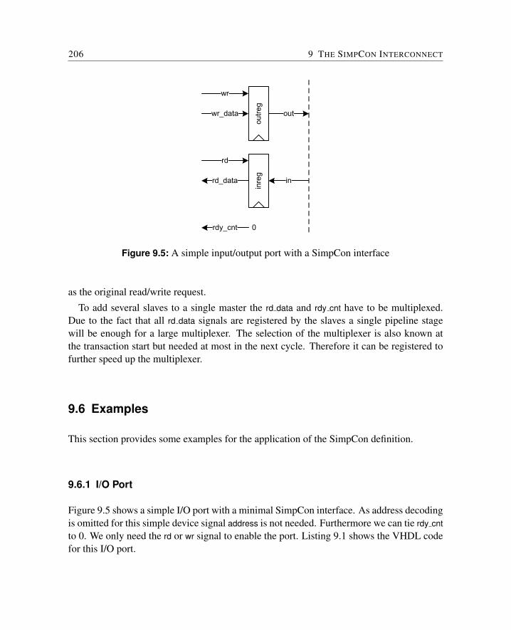
206 9 THE SIMPCON INTERCONNECT
outreg
inreg
wr_data
wr
rd
rd_data
rdy_cnt
out
in
0
Figure 9.5: A simple input/output port with a SimpCon interface
as the original read/write request.
To add several slaves to a single master the rd data and rdy cnt have to be multiplexed.Due to the fact that all rd data signals are registered by the slaves a single pipeline stagewill be enough for a large multiplexer. The selection of the multiplexer is also known atthe transaction start but needed at most in the next cycle. Therefore it can be registered tofurther speed up the multiplexer.
9.6 Examples
This section provides some examples for the application of the SimpCon definition.
9.6.1 I/O Port
Figure 9.5 shows a simple I/O port with a minimal SimpCon interface. As address decodingis omitted for this simple device signal address is not needed. Furthermore we can tie rdy cntto 0. We only need the rd or wr signal to enable the port. Listing 9.1 shows the VHDL codefor this I/O port.
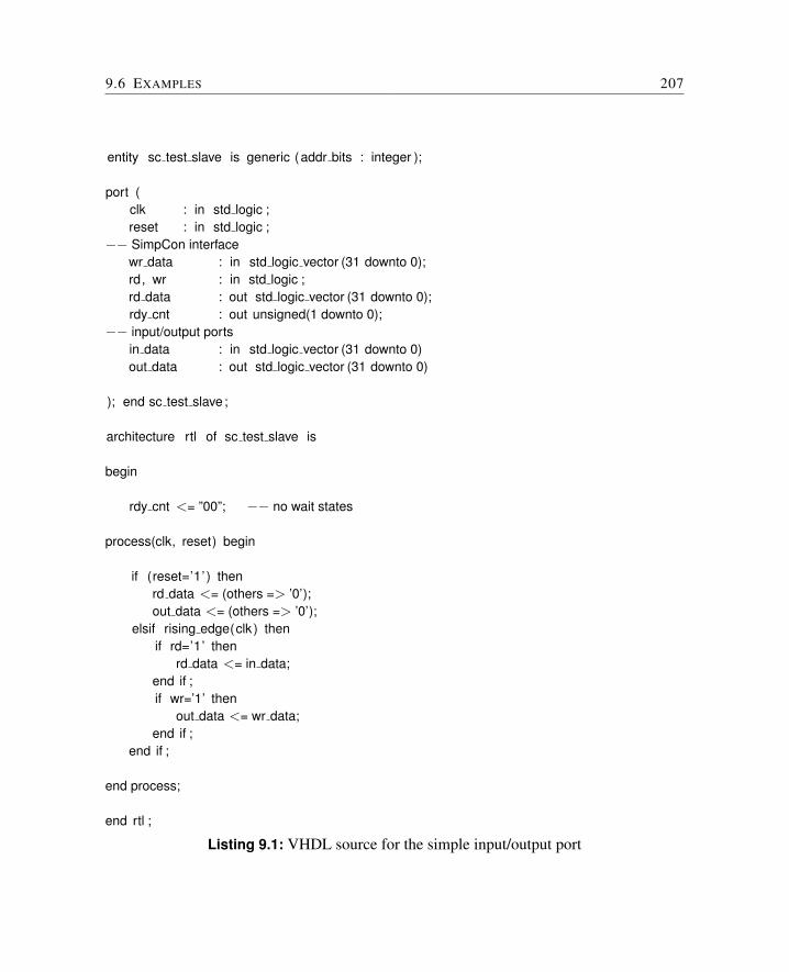
9.6 EXAMPLES 207
entity sc test slave is generic (addr bits : integer );
port (clk : in std logic ;reset : in std logic ;
−− SimpCon interfacewr data : in std logic vector (31 downto 0);rd, wr : in std logic ;rd data : out std logic vector (31 downto 0);rdy cnt : out unsigned(1 downto 0);
−− input/output portsin data : in std logic vector (31 downto 0)out data : out std logic vector (31 downto 0)
); end sc test slave ;
architecture rtl of sc test slave is
begin
rdy cnt <= ”00”; −− no wait states
process(clk, reset) begin
if (reset=’1’ ) thenrd data <= (others => ’0’);out data <= (others => ’0’);
elsif rising edge(clk ) thenif rd=’1’ then
rd data <= in data;end if ;if wr=’1’ then
out data <= wr data;end if ;
end if ;
end process;
end rtl ;
Listing 9.1: VHDL source for the simple input/output port
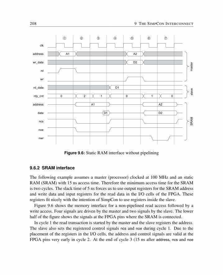
208 9 THE SIMPCON INTERCONNECT
A1
clk
address
rd
rd_data
rdy_cnt 2 1
1 2 3 4 5 6 7
wr_data
wr
address
data
ncs
noe
nwr
A1
D1
00
A2
D2
1 0
A2
D2
D1
master
slave
SRAM
Figure 9.6: Static RAM interface without pipelining
9.6.2 SRAM interface
The following example assumes a master (processor) clocked at 100 MHz and an staticRAM (SRAM) with 15 ns access time. Therefore the minimum access time for the SRAMis two cycles. The slack time of 5 ns forces us to use output registers for the SRAM addressand write data and input registers for the read data in the I/O cells of the FPGA. Theseregisters fit nicely with the intention of SimpCon to use registers inside the slave.
Figure 9.6 shows the memory interface for a non-pipelined read access followed by awrite access. Four signals are driven by the master and two signals by the slave. The lowerhalf of the figure shows the signals at the FPGA pins where the SRAM is connected.
In cycle 1 the read transaction is started by the master and the slave registers the address.The slave also sets the registered control signals ncs and noe during cycle 1. Due to theplacement of the registers in the I/O cells, the address and control signals are valid at theFPGA pins very early in cycle 2. At the end of cycle 3 (15 ns after address, ncs and noe
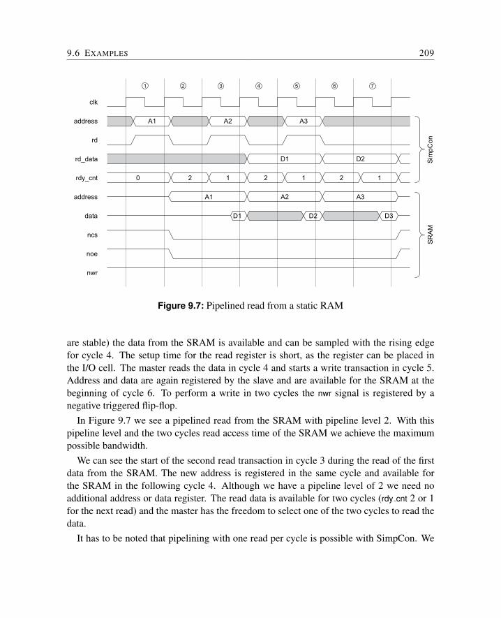
9.6 EXAMPLES 209
A1
clk
address
rd_data
1 2 3 4 5 6 7
rd
rdy_cnt
address
data
ncs
noe
nwr
A1
D1
A3
A3
SimpCon
SRAM
0 2 1 2 1 2 1
D1 D2
A2
A2
D2 D3
Figure 9.7: Pipelined read from a static RAM
are stable) the data from the SRAM is available and can be sampled with the rising edgefor cycle 4. The setup time for the read register is short, as the register can be placed inthe I/O cell. The master reads the data in cycle 4 and starts a write transaction in cycle 5.Address and data are again registered by the slave and are available for the SRAM at thebeginning of cycle 6. To perform a write in two cycles the nwr signal is registered by anegative triggered flip-flop.
In Figure 9.7 we see a pipelined read from the SRAM with pipeline level 2. With thispipeline level and the two cycles read access time of the SRAM we achieve the maximumpossible bandwidth.
We can see the start of the second read transaction in cycle 3 during the read of the firstdata from the SRAM. The new address is registered in the same cycle and available forthe SRAM in the following cycle 4. Although we have a pipeline level of 2 we need noadditional address or data register. The read data is available for two cycles (rdy cnt 2 or 1for the next read) and the master has the freedom to select one of the two cycles to read thedata.
It has to be noted that pipelining with one read per cycle is possible with SimpCon. We
210 9 THE SIMPCON INTERCONNECT
just showed a 2 cycle slave in this example. For a SDRAM memory interface the readycounter will stay either at 2 or 1 during the single cycle reads (depending on the slavepipeline level). It will go down to 0 only for the last data word to read.
9.7 Available VHDL Files
Besides the SimpCon documentation, some example VHDL files for slave devices andbridges are available from http://opencores.org/?do=project&who=simpcon. Allcomponents are also part of the standard JOP distribution.
9.7.1 Components
• sc pack.vhd defines VHDL records and some constants.
• sc test slave.vhd is a very simple SimpCon device. A counter to be read out and aregister that can be written and read. There is no connection to the outer world. Thisexample can be used as basis for a new SimpCon device.
• sc sram16.vhd is a memory controller for 16-bit SRAM.
• sc sram32.vhd is a memory controller for 32-bit SRAM.
• sc sram32 flash.vhd is a memory controller for 32-bit SRAM, a NOR Flash, and aNAND Flash as used in the Cycore FPGA board for JOP.
• sc uart.vhd is a simple UART with configurable baud rate and FIFO width.
• sc usb.vhd is an interface to the parallel port of the FTDI 2232 USB chip. The registerdefinition is identical to the UART and the USB connection can be used as a drop inreplacement for a UART.
• sc isa.vhd interfaces the old ISA bus. It can be used for the popular CS8900 Ethernetchip.
• sc sigdel.vhd is a configurable sigma-delta ADC for an FPGA that needs just twoexternal components: a capacitor and a resistor.
• sc fpu.vhd provides an interface to the 32-bit FPU available at www.opencores.org.
• sc arbiter *.vhd different zero cycle SimpCon arbiters for CMP systems written byChristof Pitter [99].
9.8 WHY A NEW INTERCONNECTION STANDARD? 211
9.7.2 Bridges
• sc2wb.vhd is a SimpCon/Wishbone [94] bridge.
• sc2avalon.vhd is a SimpCon/Avalon [4] bridge to integrate a SimpCon based designwith Altera’s SOPC Builder [5].
• sc2ahbsl.vhd provides an interface to AHB slaves as defined in Gaisler’s GRLIB [45].Many of the available GPL AHB modules from the GRLIB can be used in a SimpConbased design.
9.8 Why a New Interconnection Standard?
There are many interconnection standards available for SoC designs. The natural questionis: Why propose a new one? The answer is given in the following section. In summary, theavailable standards are still in the tradition of backplane busses and do not fit very well forpipelined on-chip interconnections.
9.8.1 Common SoC Interconnections
Several point-to-point and bus standards have been proposed. The following section givesa brief overview of common SoC interconnection standards.
The Advanced Microcontroller Bus Architecture (AMBA) [7] is the interconnectiondefinition from ARM. The specification defines three different busses: Advanced High-performance Bus (AHB), Advanced System Bus (ASB), and Advanced Peripheral Bus(APB). The AHB is used to connect on-chip memory, cache, and external memory to theprocessor. Peripheral devices are connected to the APB. A bridge connects the AHB tothe lower bandwidth APB. An AHB bus transfer can be one cycle at burst operation. Withthe APB a bus transfer requires two cycles and no burst mode is available. Peripheral buscycles with wait states are added in the version 3 of the APB specification. ASB is thepredecessor of AHB and is not recommended for new designs (ASB uses both clock phasesfor the bus signals – very uncommon for today’s synchronous designs). The AMBA 3 AXI(Advanced eXtensible Interface) [8] is the latest extension to AMBA. AXI introduces out-of-order transaction completion with the help of a 4 bit transaction ID tag. A ready signalacknowledges the transaction start. The master has to hold the transaction information (e.g.address) until the interconnect signals ready. This enhancement ruins the elegant singlecycle address phase from the original AHB specification.
212 9 THE SIMPCON INTERCONNECT
Wishbone [94] is a public domain standard used by several open-source IP cores. TheWishbone interface specification is still in the tradition of microcomputer or backplanebusses. However, for a SoC interconnect, which is usually point-to-point,3 this is not thebest approach. The master is requested to hold the address and data valid through the wholeread or write cycle. This complicates the connection to a master that has the data valid onlyfor one cycle. In this case the address and data have to be registered before the Wishboneconnect or an expensive (time and resources) multiplexer has to be used. A register resultsin one additional cycle latency. A better approach would be to register the address anddata in the slave. In that case the address decoding in the slave can be performed in thesame cycle as the address is registered. A similar issue, with respect to the master, existsfor the output data from the slave: As it is only valid for a single cycle, the data has to beregistered by the master when the master is not reading it immediately. Therefore, the slaveshould keep the last valid data at its output even when the Wishbone strobe signal (wb.stb)is not assigned anymore. Holding the data in the slave is usually for free from the hardwarecomplexity – it is just a specification issue. In the Wishbone specification there is no way toperform pipelined read or write. However, for blocked memory transfers (e.g. cache load)this is the usual way to achieve good performance.
The Avalon [4] interface specification is provided by Altera for a system-on-a-programmable-chip (SOPC) interconnection. Avalon defines a great range of inter-connection devices ranging from a simple asynchronous interface intended for direct staticRAM connection up to sophisticated pipeline transfers with variable latencies. This greatflexibility provides an easy path to connect a peripheral device to Avalon. How is thisflexibility possible? The Avalon Switch Fabric translates between all those different inter-connection types. The switch fabric is generated by Altera’s SOPC Builder tool. However,it seems that this switch fabric is Altera proprietary, thus tying this specification to AlteraFPGAs.
The On-Chip Peripheral Bus (OPB) [68] is an open standard provided by IBM and usedby Xilinx. The OPB specifies a bus for multiple masters and slaves. The implementationof the bus is not directly defined in the specification. A distributed ring, a centralizedmultiplexer, or a centralized AND/OR network are suggested. Xilinx uses the AND/ORapproach and all masters and slaves must drive the data busses to zero when inactive.
Sonics Inc. defined the Open Core Protocol (OCP) [91] as an open, freely availablestandard. The standard is now handled by the OCP International Partnership4.
3Multiplexers are used instead of busses to connect several slaves and masters.4www.ocpip.org
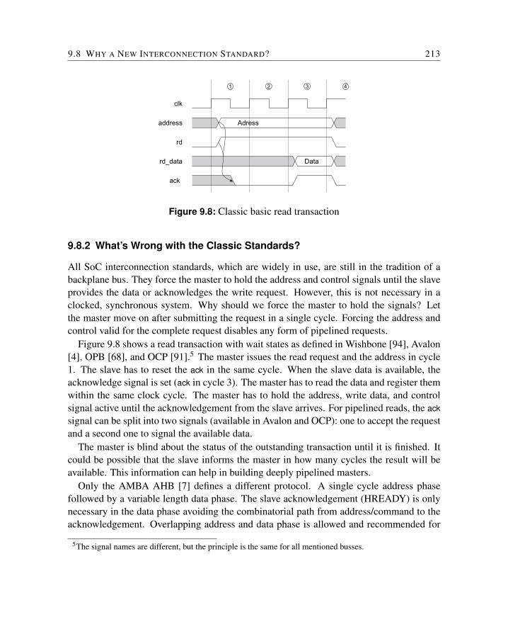
9.8 WHY A NEW INTERCONNECTION STANDARD? 213
Adress
Data
clk
address
rd
rd_data
ack
1 2 3 4
Figure 9.8: Classic basic read transaction
9.8.2 What’s Wrong with the Classic Standards?
All SoC interconnection standards, which are widely in use, are still in the tradition of abackplane bus. They force the master to hold the address and control signals until the slaveprovides the data or acknowledges the write request. However, this is not necessary in aclocked, synchronous system. Why should we force the master to hold the signals? Letthe master move on after submitting the request in a single cycle. Forcing the address andcontrol valid for the complete request disables any form of pipelined requests.
Figure 9.8 shows a read transaction with wait states as defined in Wishbone [94], Avalon[4], OPB [68], and OCP [91].5 The master issues the read request and the address in cycle1. The slave has to reset the ack in the same cycle. When the slave data is available, theacknowledge signal is set (ack in cycle 3). The master has to read the data and register themwithin the same clock cycle. The master has to hold the address, write data, and controlsignal active until the acknowledgement from the slave arrives. For pipelined reads, the acksignal can be split into two signals (available in Avalon and OCP): one to accept the requestand a second one to signal the available data.
The master is blind about the status of the outstanding transaction until it is finished. Itcould be possible that the slave informs the master in how many cycles the result will beavailable. This information can help in building deeply pipelined masters.
Only the AMBA AHB [7] defines a different protocol. A single cycle address phasefollowed by a variable length data phase. The slave acknowledgement (HREADY) is onlynecessary in the data phase avoiding the combinatorial path from address/command to theacknowledgement. Overlapping address and data phase is allowed and recommended for
5The signal names are different, but the principle is the same for all mentioned busses.
214 9 THE SIMPCON INTERCONNECT
high performance. Compared to SimpCon, AMBA AHB allows for single stage pipelining,whereas SimpCon makes multi-stage pipelining possible using the ready counter (rdy cnt).The rdy cnt signal defines the delay between the address and the data on a read, signalled bythe slave. Therefore, the pipeline depth of the bus and the slaves is only limited by the bitwidth of rdy cnt.
Another issue with all interconnection standards is the single cycle availability of theread data at the slaves. Why not keep the read data valid as long as there is no new readdata available? This feature would allow the master to be more flexible when to read thedata. It would allow issuing a read command and then continuing with other instructions –a feature known as data pre-fetching to hide long latencies.
The last argument sounds contradictory to the first argument: provide the transaction dataat the master just for a single cycle, but request the slave to hold the data for several cycles.However, it is motivated by the need to free up the master, keep it moving, and move the datahold (register) burden into the slave. As data processing bottlenecks are usually found inthe master devices, it sounds natural to move as much work as possible to the slave devicesto free up the master.
Avalon, Wishbone, and OPB provide a single cycle latency access to slaves due to thepossibility of acknowledging a request in the same cycle. However, this feature is a scalingissue for larger systems. There is a combinatorial path from master address/command toaddress decoding, slave decision on ack, slave ack multiplexing back to the master and themaster decision to hold address/command or read the data and continue. Also, the slaveoutput data multiplexer is on a combinatorial path from the master address.
AMBA, AHB, and SimpCon avoid this scaling issue by requesting the acknowledge inthe cycle following the command. In SimpCon and AMBA, the select for the read datamultiplexer can be registered as the read address is known at least one cycle before thedata is available. The later acknowledgement results in a minor drawback on SimpConand AMBA (nothing is for free): It is not possible to perform a single cycle read or writewithout pipelining. A single, non pipelined transaction takes two cycles without a waitstate. However, a single cycle read transaction is only possible for very simple slaves. Mostnon-trivial slaves (e.g. memory interfaces) will not allow a single cycle access anyway.
9.8.3 Evaluation
We compare the SimpCon interface with the AMBA and the Avalon interface as two ex-amples of common interconnection standards. As an evaluation example, we interface anexternal asynchronous SRAM with a tight timing. The system is clocked at 100 MHz andthe access time for the SRAM is 15 ns. Therefore, there are 5 ns available for on-chip reg-
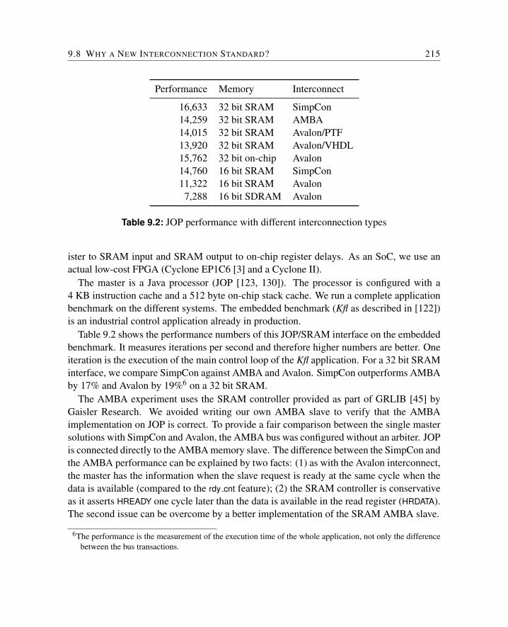
9.8 WHY A NEW INTERCONNECTION STANDARD? 215
Performance Memory Interconnect
16,633 32 bit SRAM SimpCon14,259 32 bit SRAM AMBA14,015 32 bit SRAM Avalon/PTF13,920 32 bit SRAM Avalon/VHDL15,762 32 bit on-chip Avalon14,760 16 bit SRAM SimpCon11,322 16 bit SRAM Avalon
7,288 16 bit SDRAM Avalon
Table 9.2: JOP performance with different interconnection types
ister to SRAM input and SRAM output to on-chip register delays. As an SoC, we use anactual low-cost FPGA (Cyclone EP1C6 [3] and a Cyclone II).
The master is a Java processor (JOP [123, 130]). The processor is configured with a4 KB instruction cache and a 512 byte on-chip stack cache. We run a complete applicationbenchmark on the different systems. The embedded benchmark (Kfl as described in [122])is an industrial control application already in production.
Table 9.2 shows the performance numbers of this JOP/SRAM interface on the embeddedbenchmark. It measures iterations per second and therefore higher numbers are better. Oneiteration is the execution of the main control loop of the Kfl application. For a 32 bit SRAMinterface, we compare SimpCon against AMBA and Avalon. SimpCon outperforms AMBAby 17% and Avalon by 19%6 on a 32 bit SRAM.
The AMBA experiment uses the SRAM controller provided as part of GRLIB [45] byGaisler Research. We avoided writing our own AMBA slave to verify that the AMBAimplementation on JOP is correct. To provide a fair comparison between the single mastersolutions with SimpCon and Avalon, the AMBA bus was configured without an arbiter. JOPis connected directly to the AMBA memory slave. The difference between the SimpCon andthe AMBA performance can be explained by two facts: (1) as with the Avalon interconnect,the master has the information when the slave request is ready at the same cycle when thedata is available (compared to the rdy cnt feature); (2) the SRAM controller is conservativeas it asserts HREADY one cycle later than the data is available in the read register (HRDATA).The second issue can be overcome by a better implementation of the SRAM AMBA slave.
6The performance is the measurement of the execution time of the whole application, not only the differencebetween the bus transactions.
216 9 THE SIMPCON INTERCONNECT
The Avalon experiment considers two versions: an SOPC Builder generated interface(PTF) to the memory and a memory interface written in VHDL. The SOPC Builder interfaceperforms slightly better than the VHDL version that generates the Avalon waitrequest signal.It is assumed that the SOPC Builder version uses fixed wait states within the switch fabric.
We also implemented an Avalon interface to a single-cycle on-chip memory. SimpConis even faster with the 32 bit off-chip SRAM than with the on-chip memory connectedvia Avalon. Furthermore, we also performed experiments with a 16 bit memory interfaceto the same SRAM. With this smaller data width the pressure on the interconnection andmemory interface is higher. As a result the difference between SimpCon and Avalon getslarger (30%) on the 16 bit SRAM interface. To complete the picture we also measured theperformance with an SDRAM memory connected to the Avalon bus. We see that the largelatency of an SDRAM is a big performance issue for the Java processor.
9.9 Summary
This chapter describes a simple (with respect to the definition and implementation) andefficient SoC interconnect [127]. The novel signal rdy cnt allows an early signalling to themaster when read data will be valid. This feature allows the master to restart a stalledpipeline earlier to react for arriving data. Furthermore, this feature also enables pipelinedbus transactions with a minimal effort on the master and the slave side.
We have compared SimpCon quantitative with AMBA and Avalon, two common in-terconnection definitions. The application benchmark shows a performance advantage ofSimpCon by 17% over AMBA and 19% over Avalon interfaces to an SRAM.
SimpCon is used as the main interconnect for the Java processor JOP in a single mas-ter, multiple salves configuration. SimpCon is also used to implement a shared memorychip-multiprocessor version of JOP. Furthermore, in a research project on time-triggerednetwork-on-chip [128] SimpCon is used as the socket to this NoC.
The author thanks Kevin Jennings and Tommy Thorn for the interesting discussionsabout SimpCon, Avalon, and on-chip interconnection in general at the Usenet newsgroupcomp.arch.fpga.
10 Chip Multiprocessing
In order to generate a small and predictable processor, several advanced and resource-consuming features (such as instruction folding or branch prediction) were omitted fromthe design. The resulting low resource usage of JOP makes it possible to integrate morethan one processor in an FPGA. Since embedded applications are naturally multi-threadedsystems, the performance can easily be enhanced using a multi-processor solution.
This chapter describes the configuration of a chip multiprocessor (CMP) version of JOP.The various SimpCon based arbiters have been developed by Christof Pitter and are de-scribed in [98, 99, 100]. A multi-processor JVM with shared memory offers research pos-sibilities such as: scheduling of Java threads and synchronization between the processorsor WCET analysis for the shared memory access.
The project file to start with is cyccmp, a configuration for three processors with a TDMAbased arbiter in the Cycore board with the EP1C12.
10.1 Memory Arbitration
A central arbiter regulates the synchronization on memory read and write operations.
10.1.1 Main Memory
Three different arbiter are available for the access policy to the main memory: prioritybased, fairness based, and a time division multiple access (TDMA) arbiter. The main mem-ory is shared between all cores.
The TDMA based memory arbiter provides a static schedule for the memory access.Therefore, access time to the memory is independent of tasks running on other cores. Theworst-case execution time (WCET) of a memory loads or stores can be calculated by consid-ering the worst-case phasing of the memory access pattern relative to the TDMA schedule[96].
In the default configuration each processor cores has an equally sized slot for the memoryaccess. The TDMA schedule can also be optimized for different utilizations of processing
218 10 CHIP MULTIPROCESSING
cores. The TDMA schedule can be optimized to distribute slack time of tasks to other taskswith a tighter deadline [136].
10.1.2 I/O Devices
Each core contains a set of local I/O devices, needed for the runtime system (e.g., timerinterrupt, lock support). The serial interface for program download and a stdio device isconnected to the first core.
For additional I/O devices two options exist: either they are connected to one core, orshared by all/some cores. The first option is useful when the bandwidth requirement of theI/O device is high. As I/O devices are memory mapped they can be connected to the mainmemory arbiter in the same way as the memory controller. In that case the I/O devices areshared between the cores and standard synchronization for the access is needed. For highbandwidth demands a dedicated arbiter for I/O devices or even for a single device can beused.
An interrupt line of an I/O device can be connected to a single core or to several cores.As interrupts can be individually disabled in software, a connection of all interrupt lines toall cores provides the most flexible solution.
10.2 Booting a CMP System
One interesting aspect of a CMP system is how the startup or boot-up is performed. Onpower-up, the FPGA starts the configuration state machine to read the FPGA configurationdata either from a Flash memory or via a download cable from the PC during the develop-ment process. When the configuration has finished, an internal reset is generated. After thisreset, microcode instructions are executed, starting from address 0. At this stage, we havenot yet loaded any application program (Java bytecode). The first sequence in microcodeperforms this task. The Java application can be loaded from an external Flash memory, viaa PC serial line, or an USB-port.
10.3 CMP SCHEDULING 219
In the next step, a minimal stack frame is generated and the special method Startup.boot()is invoked, even though some parts of the JVM are not yet setup. From now on JOP runs inJava mode. The method boot() performs the following steps:
• Send a greeting message to stdout
• Detect the size of the main memory
• Initialize the data structures for the garbage collector
• Initialize java.lang.System
• Print out JOP’s version number, detected clock speed, and memory size
• Invoke the static class initializers in a predefined order
• Invoke the main method of the application class
The boot-up process is the same for all processors until the generation of the internalreset and the execution of the first microcode instruction. From that point on, we have totake care that only one processor performs the initialization steps.
All processors in the CMP are functionally identical. Only one processor is designatedto boot-up and initialize the whole system. Therefore, it is necessary to distinguish betweenthe different CPUs. We assign a unique CPU identity number (CPU ID) to each processor.Only processor CPU0 is designated to do all the boot-up and initialization work. The otherCPUs have to wait until CPU0 completes the boot-up and initialization sequence. At thebeginning of the booting sequence, CPU0 loads the Java application. Meanwhile, all otherprocessors are waiting for an initialization finished signal of CPU0. This busy wait is per-formed in microcode. When the other CPUs are enabled, they will run the same sequenceas CPU0. Therefore, the initialization steps are guarded by a condition on the CPU ID.
10.3 CMP Scheduling
There are two possibilities to run multiple threads on the CMP system:
1. A single thread per processor
2. Several threads on each processor
220 10 CHIP MULTIPROCESSING
For the configuration of one thread per processor the scheduler does not need to bestarted. Running several threads on each core is managed via the JOP real-time threadsRtThread.
The scheduler on each core is a preemptive, priority based real-time scheduler. As eachthread gets a unique priority, no FIFO queues within priorities are needed. The best ana-lyzable real-time CMP scheduler does not allow threads to migrate between cores. Eachthread is pinned to a single core at creation. Therefore, standard scheduling analysis can beperformed on a per core base. Threads cannot migrate from one core to another one.
Similar to the uniprocessor version of JOP, the application is divided into an initializationphase and a mission phase. During the initialization phase, a predetermined core executesonly one thread that has to create all data structures and the threads for the mission phase.During transition to the mission phase all created threads are started.
The uniprocessor real-time scheduler for JOP has been enhanced to facilitate the schedul-ing of threads in the CMP configuration. Each core executes its own instance of the sched-uler. The scheduler is implemented as Runnable, which is registered as an interrupt handlerfor the core local timer interrupt. The scheduling is not tick-based. Instead, the timer in-terrupt is reprogrammed after each scheduling decision. During the mission start, the othercores and timer interrupts are enabled.
Another interesting option to use a CMP system is to execute exactly one thread percore. In this configuration scheduling overheads can be avoided and each core can reachan utilization of 100% without missing a deadline. To explore the CMP system withouta scheduler, a mechanism is provided to register objects, which implement the Runnableinterface, for each core. When the other cores are enabled, they execute the run method ofthe Runnable as their main method.
10.3.1 One Thread per Core
The first processor executes, as usual, main(). To execute code on the other cores a Runnablehas to be registered for each core. After registering those Runnables the other cores needto be started. The code in Listing 10.1 shows an example that can be found in test/cmp/Hel-loCMP.java.
10.3.2 Scheduling on the CMP System
Running several threads on each core is possible with RtThread and setting the core for eachthread with RtThread.setProcessor(nr). The example in Listing 10.2 (test/cmp/RtHelloCMP.java)shows registering of 50 threads on all available cores. On missionStart() the threads are
10.3 CMP SCHEDULING 221
distributed to the cores, a scheduler for each core registered as timer interrupt handler, andthe other cores started.
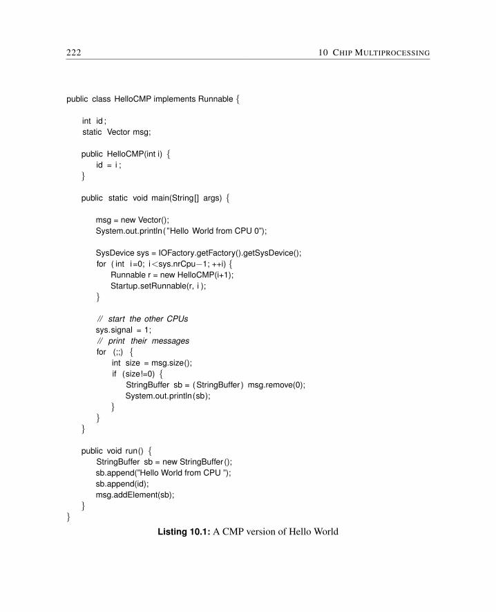
222 10 CHIP MULTIPROCESSING
public class HelloCMP implements Runnable {
int id ;static Vector msg;
public HelloCMP(int i) {id = i ;
}
public static void main(String[] args) {
msg = new Vector();System.out.println( ”Hello World from CPU 0”);
SysDevice sys = IOFactory.getFactory().getSysDevice();for ( int i=0; i<sys.nrCpu−1; ++i) {
Runnable r = new HelloCMP(i+1);Startup.setRunnable(r, i );
}
// start the other CPUssys.signal = 1;// print their messagesfor (;;) {
int size = msg.size();if (size!=0) {
StringBuffer sb = (StringBuffer ) msg.remove(0);System.out.println(sb);
}}
}
public void run() {StringBuffer sb = new StringBuffer ();sb.append(”Hello World from CPU ”);sb.append(id);msg.addElement(sb);
}}
Listing 10.1: A CMP version of Hello World
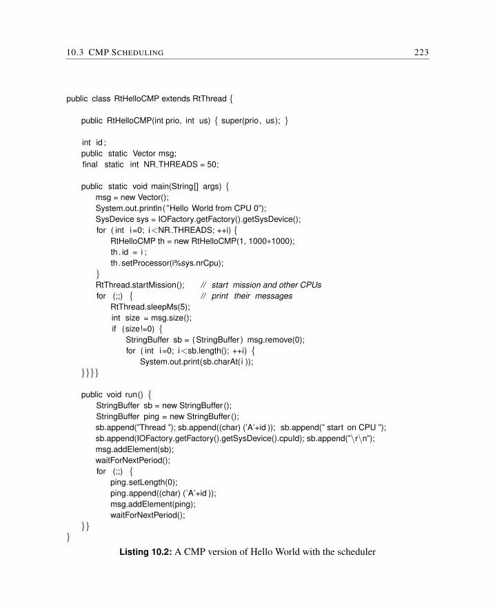
10.3 CMP SCHEDULING 223
public class RtHelloCMP extends RtThread {
public RtHelloCMP(int prio, int us) { super(prio, us); }
int id ;public static Vector msg;final static int NR THREADS = 50;
public static void main(String[] args) {msg = new Vector();System.out.println( ”Hello World from CPU 0”);SysDevice sys = IOFactory.getFactory().getSysDevice();for ( int i=0; i<NR THREADS; ++i) {
RtHelloCMP th = new RtHelloCMP(1, 1000∗1000);th . id = i ;th .setProcessor(i%sys.nrCpu);
}RtThread.startMission(); // start mission and other CPUsfor (;;) { // print their messages
RtThread.sleepMs(5);int size = msg.size();if (size!=0) {
StringBuffer sb = (StringBuffer ) msg.remove(0);for ( int i=0; i<sb.length(); ++i) {
System.out.print(sb.charAt(i ));}}}}
public void run() {StringBuffer sb = new StringBuffer ();StringBuffer ping = new StringBuffer ();sb.append(”Thread ”); sb.append((char) (’A’+id )); sb.append(” start on CPU ”);sb.append(IOFactory.getFactory().getSysDevice().cpuId); sb.append(”\r\n”);msg.addElement(sb);waitForNextPeriod();for (;;) {
ping.setLength(0);ping.append((char) (’A’+id ));msg.addElement(ping);waitForNextPeriod();
}}}
Listing 10.2: A CMP version of Hello World with the scheduler

11 Evaluation
In this chapter, we present the evaluation results for JOP. In the following section, the hard-ware platform that is used for benchmarking is described. This is followed by a comparisonof JOP’s resource usage with other soft-core processors. In Section 11.3 the performance ofa number of different solutions for embedded Java is compared with embedded applicationbenchmarks. Comparison at bytecode level can be found in [122]. This chapter concludeswith a description of real-world applications based on JOP.
11.1 Hardware Platforms
During the development of JOP and its predecessors, several different FPGA boards weredeveloped. The first experiments involved using Altera FPGAs EPF8282,EPF8452, EPF10K10 and ACEX 1K30 on boards that were connected to the printerport of a PC for configuration, download and communication. The next step was thedevelopment of a stand-alone board with FLASH memory and static RAM. This board wasdeveloped in two variants, one with an ACEX 1K50 and the other with a Cyclone EP1C6or EP1C12. Both boards are pin-compatible and are used in commercial applications ofJOP. The Cyclone board is the hardware that is used for the following evaluations.
This board is an ideal development platform for JOP. Static RAM and FLASH are con-nected via independent buses to the FPGA. All unused FPGA pins and the serial line areavailable via four connectors. The FLASH can be used to store configuration data for theFPGA and application program/data. The FPGA can be configured with a ByteBlasterMVdownload cable or loaded from the FLASH (with a small CPLD on board). As the FLASHis also connected to the FPGA, it can be programmed from the FPGA. This allows for up-grades of the Java program and even the processor core itself in the field. The board isslightly different from other FPGA prototyping boards, in that its connectors are on thebottom side. Therefore, it can be used as a module (60 mm x 48 mm), i.e. as part of a largerboard that contains the periphery. The Cyclone board contains:
• Altera Cyclone EP1C6Q240 or EP1C12Q240
• Step Down voltage regulator (1V5)
226 11 EVALUATION
• Crystal clock (20 MHz) at the PLL input (up to 640 MHz internal)
• 512 KB FLASH (for FPGA configuration and program code)
• 1 MB fast asynchronous RAM (15 ns)
• Up to 128 MB NAND FLASH
• ByteBlasterMV port
• Watchdog with a LED
• EPM7064 PLD to configure the FPGA from the FLASH on watchdog reset
• Serial interface driver (MAX3232)
• 56 general-purpose I/O pins
The RAM consists of two independent 16-bit banks (with their own address and controllines). Both RAM chips are on the bottom side of the PCB, directly under the FPGApins. As the traces are very short (under 10 mm), it is possible to use the RAMs at fullspeed without reflection problems. The two banks can be combined to form 32-bit RAM orsupport two independent CPU cores. Pictures and the schematic of the board can be foundin Appendix E.1.
The expansion board Baseio hosts the CPU module and provides a complete Java proces-sor system with Internet connection. A step down switching regulator with a large AC/DCinput range supplies the core board. All input and output pins are EMC/ESD-protectedand routed to large connectors (5.08 mm Phoenix). Analog comparators can be used tobuild sigma-delta ADCs. For FPGA projects with a network connection, a CS8900 Ether-net controller with an RJ45 connector is included on the expansion board. Pictures and theschematic of the board can be found in Appendix E.2.
11.2 Chip Area and Clock Frequency
Cost is an important issue for embedded systems. The cost of a chip is directly relatedto the die size (the cost per die is roughly proportional to the square of the die area [62]).Processors for embedded systems are therefore optimized for minimum chip size. In thissection, we will compare JOP with different processors in terms of size. One major designobjective in the development of JOP was to create a small system that can be implementedin a low-cost FPGA.
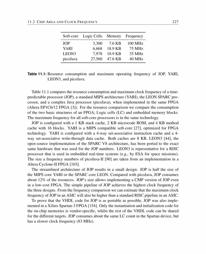
11.2 CHIP AREA AND CLOCK FREQUENCY 227
Soft-core Logic Cells Memory Frequency
JOP 3,300 7.6 KB 100 MHzYARI 6,668 18.9 KB 75 MHzLEON3 7,978 10.9 KB 35 MHzpicoJava 27,560 47.6 KB 40 MHz
Table 11.1: Resource consumption and maximum operating frequency of JOP, YARI,LEON3, and picoJava.
Table 11.1 compares the resource consumption and maximum clock frequency of a time-predictable processor (JOP), a standard MIPS architecture (YARI), the LEON SPARC pro-cessor, and a complex Java processor (picoJava), when implemented in the same FPGA(Altera EP1C6/12 FPGA [3]). For the resource comparison we compare the consumptionof the two basic structures of an FPGA; Logic cells (LC) and embedded memory blocks.The maximum frequency for all soft-core processors is in the same technology.
JOP is configured with a 1 KB stack cache, 2 KB microcode ROM, and 4 KB methodcache with 16 blocks. YARI is a MIPS compatible soft-core [27], optimized for FPGAtechnology. YARI is configured with a 4-way set-associative instruction cache and a 4-way set-associative write-through data cache. Both caches are 8 KB. LEON3 [44], theopen-source implementation of the SPARC V8 architecture, has been ported to the exactsame hardware that was used for the JOP numbers. LEON3 is representative for a RISCprocessor that is used in embedded real-time systems (e.g., by ESA for space missions).The size a frequency numbers of picoJava-II [90] are taken from an implementation in aAltera Cyclone-II FPGA [103].
The streamlined architecture of JOP results in a small design: JOP is half the size ofthe MIPS core YARI or the SPARC core LEON. Compared with picoJava, JOP consumesabout 12% of the resources. JOP’s size allows implementing a CMP version of JOP evenin a low-cost FPGA. The simple pipeline of JOP achieves the highest clock frequency ofthe three designs. From the frequency comparison we can estimate that the maximum clockfrequency of JOP in an ASIC will also be higher than a standard RISC pipeline in an ASIC.
To prove that the VHDL code for JOP is as portable as possible, JOP was also imple-mented in a Xilinx Spartan-3 FPGA [154]. Only the instantiation and initialization code forthe on-chip memories is vendor-specific, whilst the rest of the VHDL code can be sharedfor the different targets. JOP consumes about the same LC count in the Spartan device, buthas a slower clock frequency (83 MHz).
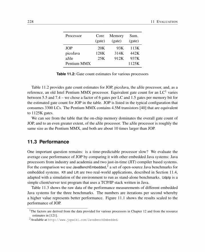
228 11 EVALUATION
Processor Core Memory Sum.(gate) (gate) (gate)
JOP 20K 93K 113KpicoJava 128K 314K 442KaJile 25K 912K 937KPentium MMX 1125K
Table 11.2: Gate count estimates for various processors
Table 11.2 provides gate count estimates for JOP, picoJava, the aJile processor, and, as areference, an old Intel Pentium MMX processor. Equivalent gate count for an LC1 variesbetween 5.5 and 7.4 – we chose a factor of 6 gates per LC and 1.5 gates per memory bit forthe estimated gate count for JOP in the table. JOP is listed in the typical configuration thatconsumes 3300 LCs. The Pentium MMX contains 4.5M transistors [40] that are equivalentto 1125K gates.
We can see from the table that the on-chip memory dominates the overall gate count ofJOP, and to an even greater extent, of the aJile processor. The aJile processor is roughly thesame size as the Pentium MMX, and both are about 10 times larger than JOP.
11.3 Performance
One important question remains: is a time-predictable processor slow? We evaluate theaverage case performance of JOP by comparing it with other embedded Java systems: Javaprocessors from industry and academia and two just-in-time (JIT) compiler based systems.For the comparison we use JavaBenchEmbedded,2 a set of open-source Java benchmarks forembedded systems. Kfl and Lift are two real-world applications, described in Section 11.4,adapted with a simulation of the environment to run as stand-alone benchmarks. UdpIp is asimple client/server test program that uses a TCP/IP stack written in Java.
Table 11.3 shows the raw data of the performance measurements of different embeddedJava systems for the three benchmarks. The numbers are iterations per second wherebya higher value represents better performance. Figure 11.1 shows the results scaled to theperformance of JOP.
1The factors are derived from the data provided for various processors in Chapter 12 and from the resourceestimates in [121].
2Available at http://www.jopwiki.com/JavaBenchEmbedded.
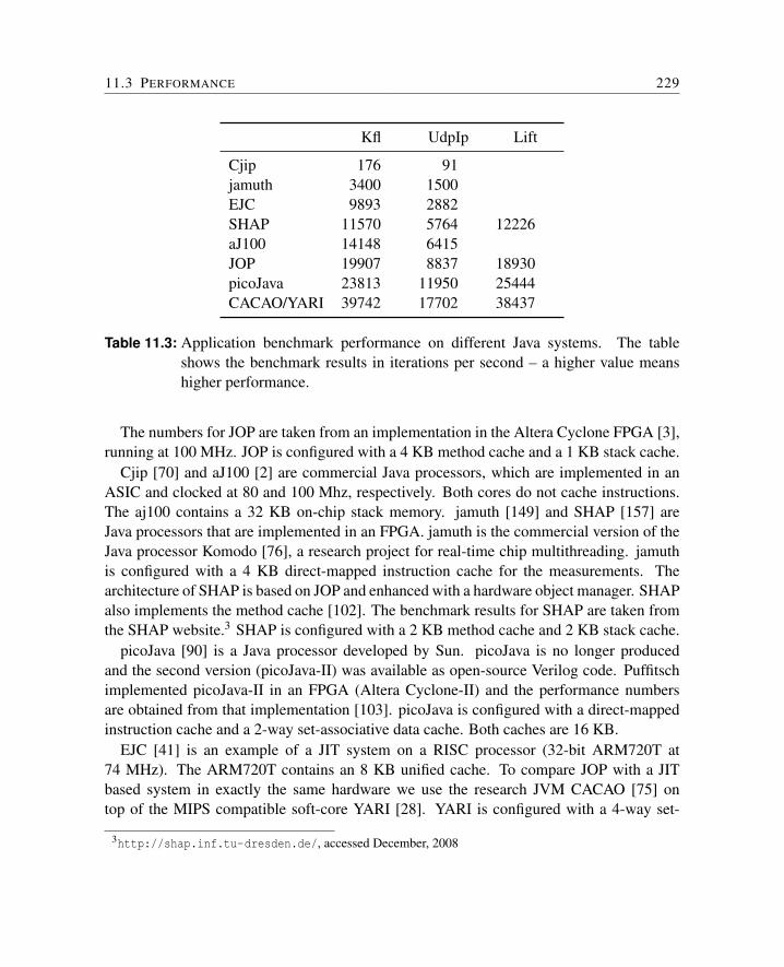
11.3 PERFORMANCE 229
Kfl UdpIp Lift
Cjip 176 91jamuth 3400 1500EJC 9893 2882SHAP 11570 5764 12226aJ100 14148 6415JOP 19907 8837 18930picoJava 23813 11950 25444CACAO/YARI 39742 17702 38437
Table 11.3: Application benchmark performance on different Java systems. The tableshows the benchmark results in iterations per second – a higher value meanshigher performance.
The numbers for JOP are taken from an implementation in the Altera Cyclone FPGA [3],running at 100 MHz. JOP is configured with a 4 KB method cache and a 1 KB stack cache.
Cjip [70] and aJ100 [2] are commercial Java processors, which are implemented in anASIC and clocked at 80 and 100 Mhz, respectively. Both cores do not cache instructions.The aj100 contains a 32 KB on-chip stack memory. jamuth [149] and SHAP [157] areJava processors that are implemented in an FPGA. jamuth is the commercial version of theJava processor Komodo [76], a research project for real-time chip multithreading. jamuthis configured with a 4 KB direct-mapped instruction cache for the measurements. Thearchitecture of SHAP is based on JOP and enhanced with a hardware object manager. SHAPalso implements the method cache [102]. The benchmark results for SHAP are taken fromthe SHAP website.3 SHAP is configured with a 2 KB method cache and 2 KB stack cache.
picoJava [90] is a Java processor developed by Sun. picoJava is no longer producedand the second version (picoJava-II) was available as open-source Verilog code. Puffitschimplemented picoJava-II in an FPGA (Altera Cyclone-II) and the performance numbersare obtained from that implementation [103]. picoJava is configured with a direct-mappedinstruction cache and a 2-way set-associative data cache. Both caches are 16 KB.
EJC [41] is an example of a JIT system on a RISC processor (32-bit ARM720T at74 MHz). The ARM720T contains an 8 KB unified cache. To compare JOP with a JITbased system in exactly the same hardware we use the research JVM CACAO [75] ontop of the MIPS compatible soft-core YARI [28]. YARI is configured with a 4-way set-
3http://shap.inf.tu-dresden.de/, accessed December, 2008
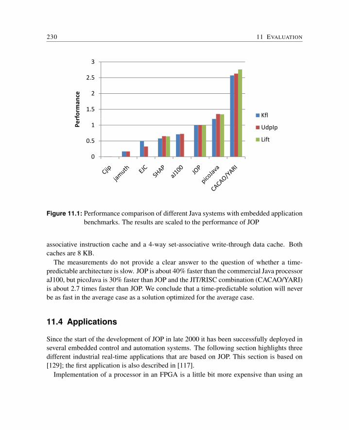
230 11 EVALUATION
1.5
2
2.5
3
rforman
ce
Kfl
0
0.5
1Per
UdpIp
Lift
Figure 11.1: Performance comparison of different Java systems with embedded applicationbenchmarks. The results are scaled to the performance of JOP
associative instruction cache and a 4-way set-associative write-through data cache. Bothcaches are 8 KB.
The measurements do not provide a clear answer to the question of whether a time-predictable architecture is slow. JOP is about 40% faster than the commercial Java processoraJ100, but picoJava is 30% faster than JOP and the JIT/RISC combination (CACAO/YARI)is about 2.7 times faster than JOP. We conclude that a time-predictable solution will neverbe as fast in the average case as a solution optimized for the average case.
11.4 Applications
Since the start of the development of JOP in late 2000 it has been successfully deployed inseveral embedded control and automation systems. The following section highlights threedifferent industrial real-time applications that are based on JOP. This section is based on[129]; the first application is also described in [117].
Implementation of a processor in an FPGA is a little bit more expensive than using an
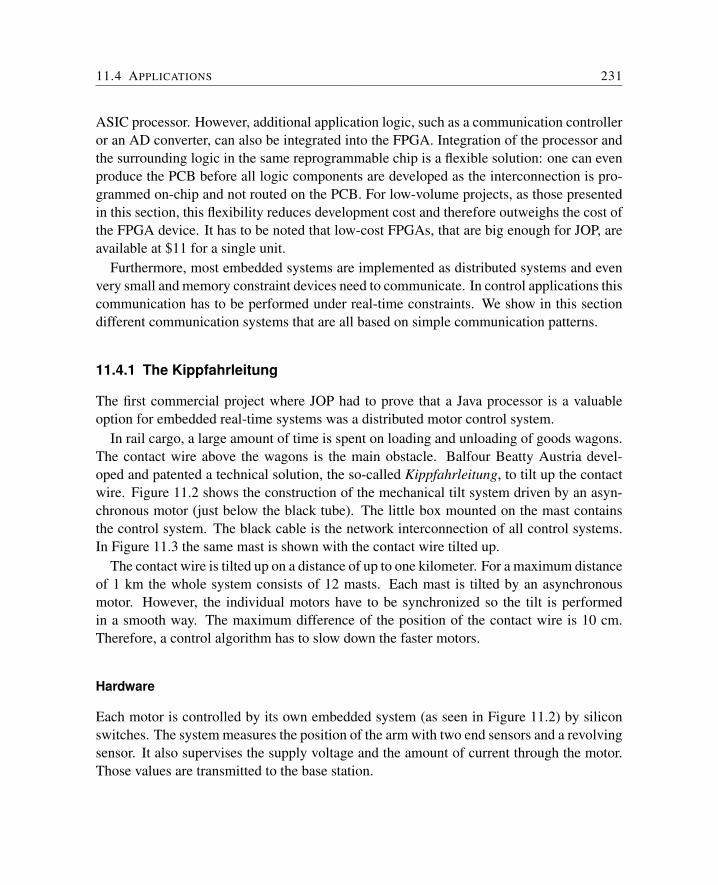
11.4 APPLICATIONS 231
ASIC processor. However, additional application logic, such as a communication controlleror an AD converter, can also be integrated into the FPGA. Integration of the processor andthe surrounding logic in the same reprogrammable chip is a flexible solution: one can evenproduce the PCB before all logic components are developed as the interconnection is pro-grammed on-chip and not routed on the PCB. For low-volume projects, as those presentedin this section, this flexibility reduces development cost and therefore outweighs the cost ofthe FPGA device. It has to be noted that low-cost FPGAs, that are big enough for JOP, areavailable at $11 for a single unit.
Furthermore, most embedded systems are implemented as distributed systems and evenvery small and memory constraint devices need to communicate. In control applications thiscommunication has to be performed under real-time constraints. We show in this sectiondifferent communication systems that are all based on simple communication patterns.
11.4.1 The Kippfahrleitung
The first commercial project where JOP had to prove that a Java processor is a valuableoption for embedded real-time systems was a distributed motor control system.
In rail cargo, a large amount of time is spent on loading and unloading of goods wagons.The contact wire above the wagons is the main obstacle. Balfour Beatty Austria devel-oped and patented a technical solution, the so-called Kippfahrleitung, to tilt up the contactwire. Figure 11.2 shows the construction of the mechanical tilt system driven by an asyn-chronous motor (just below the black tube). The little box mounted on the mast containsthe control system. The black cable is the network interconnection of all control systems.In Figure 11.3 the same mast is shown with the contact wire tilted up.
The contact wire is tilted up on a distance of up to one kilometer. For a maximum distanceof 1 km the whole system consists of 12 masts. Each mast is tilted by an asynchronousmotor. However, the individual motors have to be synchronized so the tilt is performedin a smooth way. The maximum difference of the position of the contact wire is 10 cm.Therefore, a control algorithm has to slow down the faster motors.
Hardware
Each motor is controlled by its own embedded system (as seen in Figure 11.2) by siliconswitches. The system measures the position of the arm with two end sensors and a revolvingsensor. It also supervises the supply voltage and the amount of current through the motor.Those values are transmitted to the base station.
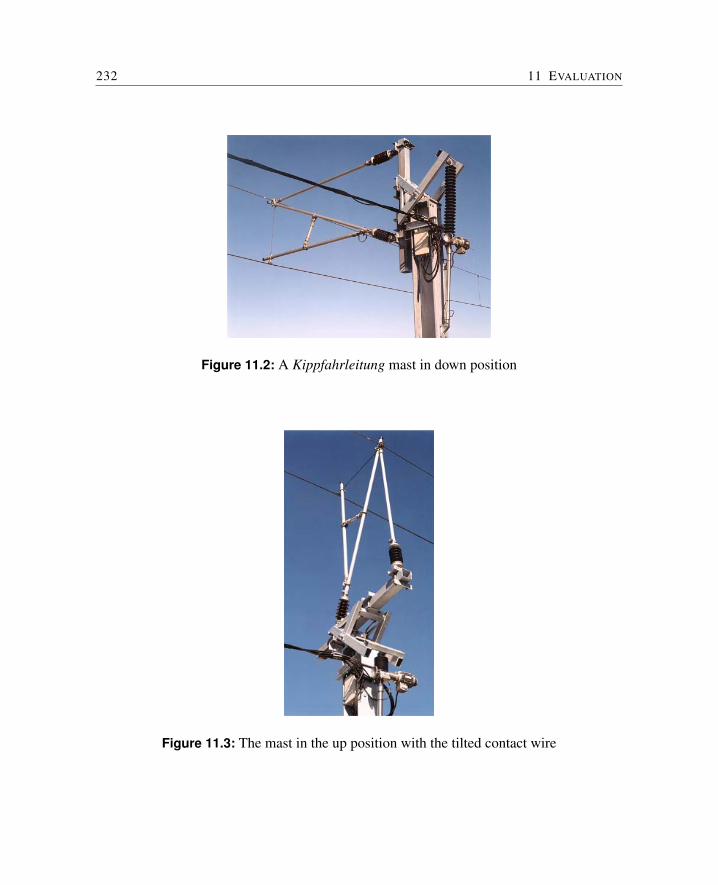
232 11 EVALUATION
Figure 11.2: A Kippfahrleitung mast in down position
Figure 11.3: The mast in the up position with the tilted contact wire
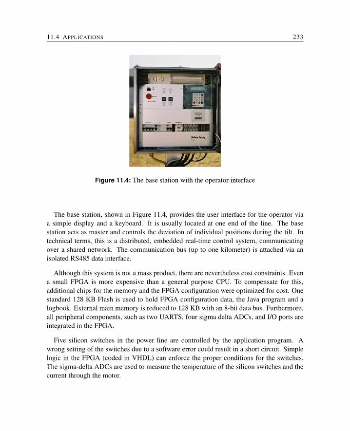
11.4 APPLICATIONS 233
Figure 11.4: The base station with the operator interface
The base station, shown in Figure 11.4, provides the user interface for the operator viaa simple display and a keyboard. It is usually located at one end of the line. The basestation acts as master and controls the deviation of individual positions during the tilt. Intechnical terms, this is a distributed, embedded real-time control system, communicatingover a shared network. The communication bus (up to one kilometer) is attached via anisolated RS485 data interface.
Although this system is not a mass product, there are nevertheless cost constraints. Evena small FPGA is more expensive than a general purpose CPU. To compensate for this,additional chips for the memory and the FPGA configuration were optimized for cost. Onestandard 128 KB Flash is used to hold FPGA configuration data, the Java program and alogbook. External main memory is reduced to 128 KB with an 8-bit data bus. Furthermore,all peripheral components, such as two UARTS, four sigma delta ADCs, and I/O ports areintegrated in the FPGA.
Five silicon switches in the power line are controlled by the application program. Awrong setting of the switches due to a software error could result in a short circuit. Simplelogic in the FPGA (coded in VHDL) can enforce the proper conditions for the switches.The sigma-delta ADCs are used to measure the temperature of the silicon switches and thecurrent through the motor.
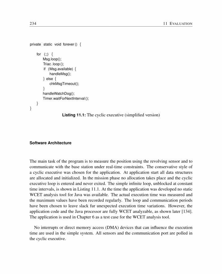
234 11 EVALUATION
private static void forever () {
for (;;) {Msg.loop();Triac .loop ();if (Msg.available) {
handleMsg();} else {
chkMsgTimeout();}handleWatchDog();Timer.waitForNextInterval ();
}}
Listing 11.1: The cyclic executive (simplified version)
Software Architecture
The main task of the program is to measure the position using the revolving sensor and tocommunicate with the base station under real-time constraints. The conservative style ofa cyclic executive was chosen for the application. At application start all data structuresare allocated and initialized. In the mission phase no allocation takes place and the cyclicexecutive loop is entered and never exited. The simple infinite loop, unblocked at constanttime intervals, is shown in Listing 11.1. At the time the application was developed no staticWCET analysis tool for Java was available. The actual execution time was measured andthe maximum values have been recorded regularly. The loop and communication periodshave been chosen to leave slack fur unexpected execution time variations. However, theapplication code and the Java processor are fully WCET analyzable, as shown later [134].The application is used in Chapter 6 as a test case for the WCET analysis tool.
No interrupts or direct memory access (DMA) devices that can influence the executiontime are used in the simple system. All sensors and the communication port are polled inthe cyclic executive.
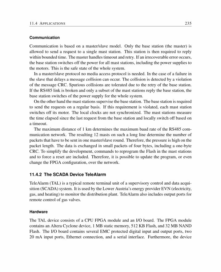
11.4 APPLICATIONS 235
Communication
Communication is based on a master/slave model. Only the base station (the master) isallowed to send a request to a single mast station. This station is then required to replywithin bounded time. The master handles timeout and retry. If an irrecoverable error occurs,the base station switches off the power for all mast stations, including the power supplies tothe motors. This is the safe state of the whole system.
In a master/slave protocol no media access protocol is needed. In the case of a failure inthe slave that delays a message collision can occur. The collision is detected by a violationof the message CRC. Spurious collisions are tolerated due to the retry of the base station.If the RS485 link is broken and only a subset of the mast stations reply the base station, thebase station switches of the power supply for the whole system.
On the other hand the mast stations supervise the base station. The base station is requiredto send the requests on a regular basis. If this requirement is violated, each mast stationswitches off its motor. The local clocks are not synchronized. The mast stations measurethe time elapsed since the last request from the base station and locally switch off based ona timeout.
The maximum distance of 1 km determines the maximum baud rate of the RS485 com-munication network. The resulting 12 masts on such a long line determine the number ofpackets that have to be sent in one master/slave round. Therefore, the pressure is high on thepacket length. The data is exchanged in small packets of four bytes, including a one-byteCRC. To simplify the development, commands to reprogram the Flash in the mast stationsand to force a reset are included. Therefore, it is possible to update the program, or evenchange the FPGA configuration, over the network.
11.4.2 The SCADA Device TeleAlarm
TeleAlarm (TAL) is a typical remote terminal unit of a supervisory control and data acqui-sition (SCADA) system. It is used by the Lower Austria’s energy provider EVN (electricity,gas, and heating) to monitor the distribution plant. TeleAlarm also includes output ports forremote control of gas valves.
Hardware
The TAL device consists of a CPU FPGA module and an I/O board. The FPGA modulecontains an Altera Cyclone device, 1 MB static memory, 512 KB Flash, and 32 MB NANDFlash. The I/O board contains several EMC protected digital input and output ports, two20 mA input ports, Ethernet connection, and a serial interface. Furthermore, the device
236 11 EVALUATION
SCADA Central System
Operator
SCADA Network
Modem Pool
Modem
TAL
Valve
Input Value
Input Value
Figure 11.5: EVN SCADA system with the modem pool and TALs as remote terminal units
performs loading of a rechargeable battery to survive power down failures. On power down,an important event for a energy provider, an alarm is sent. The rechargeable battery is alsomonitored and the device switches itself off when the minimal voltage threshold is reached.This event is sent to the SCADA system before the power is switched off.
The same hardware is also used for a different project: a lift control in an automationfactory in Turkey. The simple lift control software is now used as a test case for WCET tooldevelopment (see Chapter 6).
Communication
The communication between the TAL and the main supervisory control system is performedwith a proprietary protocol. On a value change, the TAL sends the new data to the centralsystem. Furthermore, the remote units are polled by the central system at a regular base. TheTAL itself also sends the actual state regularly. TAL can communicate via Internet/Ethernet,a modem, and via SMS to a mobile phone.
EVN uses a mixture of dial-up network and leased lines for the plant communication.The dial-up modems are hosted by EVN itself. For safety and security reason there is noconnection between the control network and the office network or the Internet.
11.4 APPLICATIONS 237
Figure 11.5 shows the SCADA system setup at EVN. Several TALs are connected viamodems to the central modem pool. The modem pool itself is connected to the centralserver. It has to be noted that there are many more TALs in the field than modems in thepool. The communication is usually very short (several seconds) and performed on demandand on a long regular interval. Not shown in the figure are additional SCADA stations andother remote terminal units from other manufacturers.
11.4.3 Support for Single Track Railway Control
Another application of JOP is in a communication device with soft real-time properties –Austrian Railways’ (OBB) new support system for single-track lines. The system helps thesuperintendent at the railway station to keep track of all trains on the track. He can submitcommands to the engine drivers of the individual trains. Furthermore, the device checks thecurrent position of the train and generates an alarm when the train enters a track segmentwithout a clearance.
At the central station all track segments are administered and controlled. When a trainenters a non-allowed segment all trains nearby are warned automatically. This warninggenerates an alarm at the locomotive and the engine driver has to perform an emergencystop.
Figure 11.6 gives an overview of the system. The display and command terminal at therailway station is connected to the Intranet of the railway company. On the right side ofthe figure a picture of the terminal that is connected to the Internet via GPRS and to a GPSreceiver is shown. Each locomotive that enters the track is equipped with either one or twoof those terminals.
It has to be noted that this system is not a safety-critical system. The communicationover a public mobile phone network is not reliable and the system is not certified for safety.The intension is just to support the superintendent and the engine drivers.
Hardware
Each locomotive is equipped with a GPS receiver, a GPRS modem, and the communicationdevice (terminal). The terminal is a custom made device. The FPGA module is the same asin TAL, only the I/O board is adapted for this application. The I/O board contains severalserial line interfaces for the GPS receiver, the GPRS modem, debug and download, anddisplay connection. Auxiliary I/O ports connected to relays are reserved for future use. Apossible extension is to stop the train automatically.
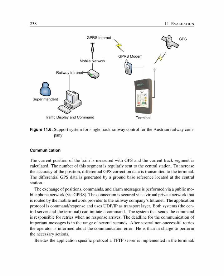
238 11 EVALUATION
Traffic Display and Command
Superintendent
Railway Intranet
Mobile Network
GPRS Internet GPS
GPRS Modem
Terminal
Figure 11.6: Support system for single track railway control for the Austrian railway com-pany
Communication
The current position of the train is measured with GPS and the current track segment iscalculated. The number of this segment is regularly sent to the central station. To increasethe accuracy of the position, differential GPS correction data is transmitted to the terminal.The differential GPS data is generated by a ground base reference located at the centralstation.
The exchange of positions, commands, and alarm messages is performed via a public mo-bile phone network (via GPRS). The connection is secured via a virtual private network thatis routed by the mobile network provider to the railway company’s Intranet. The applicationprotocol is command/response and uses UDP/IP as transport layer. Both systems (the cen-tral server and the terminal) can initiate a command. The system that sends the commandis responsible for retries when no response arrives. The deadline for the communication ofimportant messages is in the range of several seconds. After several non-successful retriesthe operator is informed about the communication error. He is than in charge to performthe necessary actions.
Besides the application specific protocol a TFTP server is implemented in the terminal.
11.4 APPLICATIONS 239
It is used to update the track data for the position detection and to upload a new versionof the software. The flexibility of the FPGA and an Internet connection to the embeddedsystem allows to upgrade the software and even the processor in the field.
11.4.4 Communication and Common Design Patterns
Although we described embedded systems from quite different application domains wehave been facing similar challenges. All systems are distributed systems and therefore needto communicate. Furthermore, they are real-time systems (at least with soft deadlines) andneed to trust the communication and perform regular checks. The issues in the design ofembedded real-time systems are quite similar in the three described projects. We found thatseveral design patterns are used over and over and describe three of them in this section.
Master/Slave Designs
Developing safe embedded systems is an exercise in reducing complexity. One paradigmto simplify embedded software development is the master/slave pattern. Usually a singlemaster is responsible to initiate commands to the slaves. The single master is also responsi-ble to handle reliable communication. The master/slave pattern also fits very well with thecommand/response pattern for the communication.
Dealing with Communication Errors
Communication is not per se reliable. The RS485 link at the Kippfahrleitung operates ina rough environment and electromagnetic influences can lead to packet loss. The TALsystem can suffer from broken phone lines. The single track control system operates ona public mobile phone network – a network without any guarantees for the GPRS datatraffic. Therefore, we have to find solutions to operate in a safe and controlled manner thedistributed system despite the chance of communication errors and failures.
Reliable communication is usually provided by the transport layer, TCP/IP in the caseof the Internet. However, the timeouts in TCP/IP are way longer than the communicationdeadlines within control systems. The approach in all three presented projects is to use adatagram oriented protocol and perform the timeout and retransmission at the applicationlevel. To simplify the timeout handling a simple command and response pattern is used.One partner sends a command and expects the response within a specific time bound. Thecommand initiator is responsible for retransmission after the timeout. The response partnerjust needs to reply to the command and does not need to remember the state of the com-munication. After several timeouts the communication error is handled by an upper layer.
240 11 EVALUATION
Either the operator is informed (in the SCADA and the railway control system) or the wholesystem is brought into a safe state (in the motor control project).
Communication errors are either transient or longer lasting. Transient communicationerrors are lost packets due to network overload or external electromagnetic influences. In acommand/response system the lost packets (either the command or the response) is detectedby a timeout on the response. A simple retransmission of the command can correct thosetransient errors.
A longer network failure, e.g. caused by a wire break, can be detected by too many trans-mission retries. In such a case the system has to enter some form of safe state. Eitherthe power is switched off or a human operator has to be informed. The individual timeoutvalues and the number of retries depend, similar to thread periods, on the controlled envi-ronment. In the Kippfahrleitung the maximum timeout is in the millisecond range, whereasin the SCADA system the timeout is several minutes.
Software Update
Correction of implementation bugs during development can be very costly when physicalaccess to the embedded system is necessary for a software update. Furthermore, a system isusually never really finished. When the system is in use the customer often finds new waysto enhance the system or requests additional features.
Therefore, an important feature of a networked embedded system is a software and pa-rameter update in the field. In the first project the software update is performed via ahome-made protocol. The other projects use the Internet protocol to some extent and there-fore TFTP is a natural choice. TFTP is a very simple protocol that can be implementedwithin about 100 lines of code. It is applicable even in very small and resource constraintembedded devices.
11.4.5 Discussion
Writing embedded control software in Java is still not very common due to the lack of smalland efficient implementations of the JVM. Our Java processor JOP is a solution for someembedded systems.
Using Java as the implementation language was a pleasure during programming and de-bugging. We did not waste many hours to hunt for pointer related bugs. The stricter (com-pared to C) type system of Java also catches many more programming errors at compiletime. However, when using Java in a small embedded system one should not expect that afull blown Java library is available. Almost all of the code had to be written without library
11.5 SUMMARY 241
support. Embedded C programmers are aware of that fact, but Java programmers are new inthe embedded domain and have to learn the difference between a PC and a 1 MB memoryembedded system.
Up to date FPGAs in embedded control systems are only used for auxiliary functions orto implement high-performance DPS algorithm directly in hardware. Using the FPGA asthe main processor is still not very common. However, combining the main processor withsome peripheral devices in the same chip can simplify the PCB layout and also reduce theproduction cost. Furthermore, a field-reprogrammable hardware device offers a great dealof flexibility: When some part of the software becomes the bottleneck, an implementation ofthat function in hardware can be a solution. Leaving some headroom in the logic resourcescan extend the lifetime of the product.
For a prototype, JOP has been attached to a time-triggered network-on-chip [128]. Itwould be an interesting exercise to implement a JOP based node in a time-triggered dis-tributed system as proposed by [73]. The combination of a real-time Java processor and areal-time network can ensure real-time characteristics for the whole system.
11.5 Summary
In this chapter, we presented an evaluation of JOP. We have seen that JOP is the smallesthardware realization of the JVM available to date. Due to the efficient implementationof the stack architecture, JOP is also smaller than a comparable RISC processor in anFPGA. Implemented in an FPGA, JOP has the highest clock frequency of all known Javaprocessors.
We compared JOP against several embedded Java systems. JOP is about 40% faster thanthe commercial Java processor aJ100, but picoJava and a JIT/RISC combination are fasterthan JOP. These results show that a time-predictable architecture does not need to be slow,but will never be as fast as an architecture optimized for average case performance.
Furthermore, we have presented three industrial applications implemented in Java onan embedded, real-time Java processor. All projects included custom designed hardware(digital functions) and the central computation unit implemented in a single FPGA. Theapplications are written in pure Java without the need for native methods in C. Java proved tobe a productive implementation language for embedded systems. Usage of JOP in four real-world applications showed that the processor is mature enough to be used in commercialprojects.

12 Related Work
Several projects provide solutions to speedup execution of Java programs in embeddedsystems. Two different approaches can be found to improve Java bytecode execution byhardware. The first type operates as a Java coprocessor in conjunction with a general-purpose microprocessor. This coprocessor is placed in the instruction fetch path of themain processor and translates Java bytecodes to sequences of instructions for the host CPUor directly executes basic Java bytecodes. The complex instructions are emulated by themain processor. Java chips in the second category replace the general-purpose CPU. Allapplications therefore have to be written in Java. While the first type enables systems withmixed code capabilities, the additional component significantly raises costs. This chaptergives an overview of the most important Java processors and coprocessors from academiaand industry.
12.1 Java Coprocessors
The simplest enhancement for Java is a translation unit, which substitutes the switch state-ment of an interpreter JVM (bytecode decoding) through hardware and/or translates simplebytecodes to a sequence of RISC instructions on the fly.
A standard JVM interpreter contains a loop with a large switch statement that decodesthe bytecode (see Listing 3.1). This switch statement is compiled to an indirect branch. Thedestinations of these indirect branches change frequently and do not benefit from branch-prediction logic. This is the main overhead for simple bytecodes on modern processors.The following approaches enhance the execution of Java programs on a standard processorthrough the substitution of the memory read and switch statement with bytecode fetch anddecode through hardware.
12.1.1 Jazelle
Jazelle [9] is an extension of the ARM 32-bit RISC processor, similar to the Thumb state(a 16-bit mode for reduced memory consumption). The Jazelle coprocessor is integrated
244 12 RELATED WORK
into the same chip as the ARM processor. The hardware bytecode decoder logic is imple-mented in less than 12K gates. It accelerates, according to ARM, some 95% of the executedbytecodes. 140 bytecodes are executed directly in hardware, while the remaining 94 are em-ulated by sequences of ARM instructions. This solution also uses code modification withquick instructions to substitute certain object-related instructions after link resolution. AllJava bytecodes, including the emulated sequences, are re-startable to enable a fast interruptresponse time.
A new ARM instruction puts the processor into the Java state. Bytecodes are fetched anddecoded in two stages, compared to a single stage in ARM state. Four registers of the ARMcore are used to cache the top stack elements. Stack spill and fill is handled automatically bythe hardware. Additional registers are reused for the Java stack pointer, the variable pointer,the constant pool pointer and locale variable 0 (the this pointer in methods). Keeping thecomplete state of the Java mode in ARM registers simplifies its integration into existingoperating systems.
12.2 Java Processors
Java Processors are primarily used in an embedded system. In such a system, Java is thenative programming language and all operating system related code, such as device drivers,are implemented in Java. Java processors are simple or extended stack architectures withan instruction set that resembles more or less the bytecodes from the JVM.
12.2.1 picoJava
Sun’s picoJava is the Java processor used as a reference for new Java processors and as thebasis for research into improving various aspects of a Java processor. Ironically, this pro-cessor was never released as a product by Sun. After Sun decided to not produce picoJavain silicon, Sun licensed picoJava to Fujitsu, IBM, LG Semicon and NEC. However, thesecompanies also did not produce a chip and Sun finally provided the full Verilog code underan open-source license.
Sun introduced the first version of picoJava [90] in 1997. The processor was targetedat the embedded systems market as a pure Java processor with restricted support of C.picoJava-I contains four pipeline stages. A redesign followed in 1999, known as picoJava-II. This is the version described below. picoJava-II was freely available with a rich set ofdocumentation [145, 146]. The probably first implementation of picoJava-II has been doneby Wolfgang Puffitsch [103, 105]. This implementation enabled the comparison of JOP
12.2 JAVA PROCESSORS 245
with picoJava-II in a similar FPGA (see Chapter 11)The architecture of picoJava is a stack-based CISC processor implementing 341 differ-
ent instructions and is the most complex Java processor available. The processor can beimplemented in about 440K gates [37]. Simple Java bytecodes are directly implementedin hardware, most of them execute in one to three cycles. Other performance critical in-structions, for instance invoking a method, are implemented in microcode. picoJava trapson the remaining complex instructions, such as creation of an object, and emulates this in-struction. A trap is rather expensive and has a minimum overhead of 16 clock cycles. Thisminimum value can only be achieved if the trap table entry is in the data cache and the firstinstruction of the trap routine is in the instruction cache. The worst-case trap latency is 926clock cycles [146]. This great variation in execution times for a trap hampers tight WCETestimates.
picoJava provides a 64-entry stack cache as a register file. The core manages this registerfile as a circular buffer, with a pointer to the top of stack. The stack management unitautomatically performs spill to and fill from the data cache to avoid overflow and underflowof the stack buffer. To provide this functionality the register file contains five memoryports. Computation needs two read ports and one write port, the concurrent spill and filloperations the two additional read and write ports. The processor core consists of followingsix pipeline stages:
Fetch: Fetch 8 bytes from the instruction cache or 4 bytes from the bus interface to the16-byte-deep prefetch buffer.
Decode: Group and precode instructions (up to 7 bytes) from the prefetch buffer. Instruc-tion folding is performed on up to four bytecodes.
Register: Read up to two operands from the register file (stack cache).
Execute: Execute simple instructions in one cycle or microcode for multi-cycle instruc-tions.
Cache: Access the data cache.
Writeback: Write the result back into the register file.
The integer unit together with the stack unit provides a mechanism, called instruction fold-ing, to speed up common code patterns found in stack architectures. When all entries arecontained in the stack cache, the picoJava core can fold these four instructions into oneRISC-style single cycle operation.
246 12 RELATED WORK
12.2.2 aJile JEMCore
aJile’s JEMCore is a direct-execution Java processor that is available as both an IP coreand a stand alone processor [2, 55]. It is based on the 32-bit JEM2 Java chip developed byRockwell-Collins. JEM2 is an enhanced version of JEM1, created in 1997 by the Rockwell-Collins Advanced Architecture Microprocessor group. Rockwell-Collins originally devel-oped JEM for avionics applications by adapting an existing design for a stack-based embed-ded processor. Rockwell-Collins decided not to sell the chip on the open market. Instead,it licensed the design exclusively to aJile Systems Inc., which was founded in 1999 byengineers from Rockwell-Collins, Centaur Technologies, Sun Microsystems, and IDT.
The core contains 24 32-bit wide registers. Six of them are used to cache the top ele-ments of the stack. The datapath consists of a 32-bit ALU, a 32-bit barrel shifter and thesupport for floating point operations (disassembly/assembly, overflow and NaN detection).The control store is a 4K by 56 ROM to hold the microcode that implements the Java byte-code. An additional RAM control store can be used for custom instructions. This feature isused to implement the basic synchronization and thread scheduling routines in microcode.It results in low execution overhead with a thread-to-thread yield in less than one µs (at100 MHz). An optional Multiple JVM Manager (MJM) supports two independent, mem-ory protected JVMs. The two JVMs execute time-sliced on the processor. According toaJile, the processor can be implemented in 25K gates (without the microcode ROM). TheMJM needs additional 10K gates.
Two silicon versions of JEM exist today: the aJ-80 and the aJ-100. Both versions com-prise a JEM2 core, the MJM, 48 KB zero wait state RAM and peripheral components, suchas timer and UART. 16 KB of the RAM is used for the writable control store. The remain-ing 32 KB is used for storage of the processor stack. The aJ-100 provides a generic 8-bit,16-bit or 32-bit external bus interface, while the aJ-80 only provides an 8-bit interface. TheaJ-100 can be clocked up to 100 MHz and the aJ-80 up to 66 MHz. The power consumptionis about 1mW per MHz.
aJile was a member of the initial Real-Time for Java Expert Group. However, up to now,no implementation of the RTSJ on top of the aJile processor emerged. One nice feature ofthis processor is its availability. Low-level access to devices via the RTSJ RawMemoryAccessobjects has been shown on the aJile processor [54]. A relatively cheap development system,the JStamp [147], was used to compare this processor with JOP.
The aJile processor is intended as a solution for real-time systems. However, no informa-tion is available about bytecode execution times. As this processor is a commercial productand has been on the market for some time, it is expected that its JVM implementation con-firms to Java standards, as defined by Sun.
12.2 JAVA PROCESSORS 247
12.2.3 Cjip
The Cjip processor [53, 70] supports multiple instruction sets, allowing Java, C, C++, andassembler to coexist. Internally, the Cjip uses 72 bit wide microcode instructions, to supportthe different instruction sets. At its core, Cjip is a 16-bit CISC architecture with on-chip36 KB ROM and 18 KB RAM for fixed and loadable microcode. Another 1 KB RAMis used for eight independent register banks, string buffer and two stack caches. Cjip isimplemented in 0.35-micron technology and can be clocked up to 66 MHz. The logic coreconsumes about 20% of the 1.4-million-transistor chip. The Cjip has 40 program controlledI/O pins, a high-speed 8 bit I/O bus with hardware DMA and an 8/16 bit DRAM interface.
The JVM is implemented largely in microcode (about 88% of the Java bytecodes). Javathread scheduling and garbage collection are implemented as processes in microcode. Mi-crocode is also used to implement virtual peripherals such as watchdog timers, display andkeyboard interfaces, sound generators, and multimedia codecs.
Microcode instructions execute in two or three cycles. A JVM bytecode requires severalmicrocode instructions. The Cjip Java instruction set and the extensions are described indetail in [69]. For example: a bytecode nop executes in 6 cycles while an iadd takes 12cycles. Conditional bytecode branches are executed in 33 to 36 cycles. Object orientedinstructions, such getfield, putfield, or invokevirtual are not part of the instruction set.
12.2.4 Lightfoot
The Lightfoot 32-bit core [35] is a hybrid 8/32-bit processor based on the Harvard architec-ture. Program memory is 8 bits wide and data memory is 32 bits wide. The core contains a3-stage pipeline with an integer ALU, a barrel shifter, and a 2-bit multiply step unit. Thereare two different stacks with the top elements implemented as registers and memory ex-tension. The data stack is used to hold temporary data – it is not used to implement theJVM stack frame. As the name implies, the return stack holds return addresses for sub-routines and it can be used as an auxiliary stack. The processor architecture specifies threedifferent instruction formats: soft bytecodes, non-returnable instructions, and single-byteinstructions that can be folded with a return instruction. The core is available in VHDL andcan be implemented in less than 30K gates. Lightfood is now part of the VS2000 TyphoonFamily Microcontroller.1
1http://www.velocitysemi.com/processors.htm
248 12 RELATED WORK
12.2.5 LavaCORE
LavaCORE [36] is another Java processor targeted at Xilinx FPGA architectures.2 It im-plements a set of instructions in hardware and firmware. Floating-point operations are notimplemented. A 32x32-bit dual-ported RAM implements a register-file. For specializedembedded applications, a tool is provided to analyze which subset of the JVM instructionsis used. The unused instructions can be omitted from the design. The core can be imple-mented in 1926 CLBs (= 3800 LCs) in a Virtex-II (2V1000-5) and runs at 20 MHz.
12.2.6 Komodo, jamuth
Komodo [158] is a multithreaded Java processor with a four-stage pipeline. It is intendedas a basis for research on real-time scheduling on a multithreaded microcontroller [76].Simple bytecodes are directly implemented, while more complex bytecodes, such as iaload,are implemented as a microcode sequence. The unique feature of Komodo is the instructionfetch unit with four independent program counters and status flags for four threads. Apriority manager is responsible for hardware real-time scheduling and can select a newthread after each bytecode instruction. The follow-up project, jamuth [149], is a commercialversion of Komodo.
Komodo’s multithreading is similar to hyper-threading in modern processors that are try-ing to hide latencies in instruction fetching. However, this feature leads to very pessimisticWCET values (in effect rendering the performance gain useless). The fact that the pipelineclock is only a quarter of the system clock also wastes a considerable amount of potentialperformance.
12.2.7 FemtoJava
FemtoJava [71] is a research project to build an application specific Java processor. Thebytecode usage of the embedded application is analyzed and a customized version of Fem-toJava is generated. FemtoJava implements up to 69 bytecode instructions for an 8 or 16bit datapath. These instructions take 3, 4, 7 or 14 cycles to execute. Analysis of smallapplications (50 to 280 byte code) showed that between 22 and 69 distinct bytecodes areused. The resulting resource usage of the FPGA varies between 1000 and 2000 LCs. Withthe reduction of the datapath to 16 bits the processor is not Java conformant.
2http://www.lavacore.com/
12.2 JAVA PROCESSORS 249
12.2.8 jHISC
The jHISC project [148] proposes a high-level instruction set architecture for Java. Thisproject is closely related to picoJava. The processor consumes 15500 LCs in an FPGAand the maximum frequency in a Xilinx Virtex FPGA is 30 MHz. According to [148] theprototype can only run simple programs and the performance is estimated with a simulation.In [155] the clocks per instruction (CPI) values for jHISC are compared against picoJavaand JOP. However, it is not explained with which application the CPI values are collected.We assume that the CPI values for picoJava and JOP are derived from the manual and donot include any effects of pipeline stalls or cache misses.
12.2.9 SHAP
The SHAP Java processor [157], although now with a different pipeline structure and hard-ware assisted garbage collection, has its roots in the JOP design. SHAP is enhanced with ahardware object manager. That unit redirects field and array access during a copy operationof the GC unit. SHAP also implements the method cache [102].
12.2.10 Azul
Azul Systems provides an impressive multiprocessor system for transactions oriented serverworkloads [15]. A single Vega chip contains 54 64-bit RISC cores, optimized for the ex-ecution of Java programs. Up to 16 Vega processors can be combined to a cache coherentmultiprocessor system with 864 processors cores, supporting up to 768 GB of shared mem-ory.

13 Summary
In this chapter we will undertake a short review of the project and summarize the contri-butions. Java for real-time systems is a new and active research area. This chapter offerssuggestions for future research, based on the described Java processor.
The research contributions made by this work are related to two areas: real-time Java andresource-constrained embedded systems.
13.1 A Real-Time Java Processor
The goal of time-predictable execution of Java programs was a first-class guiding principlethroughout the development of JOP:
• The execution time for Java bytecodes can be exactly predicted in terms of the num-ber of clock cycles. JOP is therefore a straightforward target for low-level WCETanalysis. There is no mutual dependency between consecutive bytecodes that couldresult in unbounded timing effects.
• In order to provide time-predictable execution of Java bytecodes, the processorpipeline is designed without any prefetching or queuing. This fact avoids hard-to-analyze and possibly unbounded pipeline dependencies. There are no pipeline stalls,caused by interrupts or the memory subsystem, to complicate the WCET analysis.
• A pipelined processor architecture calls for higher memory bandwidth. A standardtechnique to avoid processing bottlenecks due to the higher memory bandwidth iscaching. However, standard cache organizations improve the average execution timebut are difficult to predict for WCET analysis. Two time-predictable caches are im-plemented in JOP: a stack cache as a substitution for the data cache and a methodcache to cache the instructions.
As the stack is a heavily accessed memory region, the stack – or part of it – is placedin local memory. This part of the stack is referred to as the stack cache and described
252 13 SUMMARY
in Section 4.4. Fill and spill of the stack cache is subjected to microcode control andtherefore time-predictable.
In Section 4.5, a novel way to organize an instruction cache, as method cache, isgiven. The cache stores complete methods, and cache misses only occur on methodinvocation and return. Cache block replacement depends on the call tree, instead ofinstruction addresses. This method cache is easy to analyze with respect to worst-case behavior and still provides substantial performance gain when compared to asolution without an instruction cache.
• The time-predictable processor described above provides the basis for real-time Java.To enable real-time Java to operate on resource-constrained devices, a simple real-time profile was defined in Section 5.1 and implemented in Java on JOP. The beautyof this approach is in implementing functions usually associated with an RTOS inJava. This means that real-time Java is not based on an RTOS, and therefore notrestricted to the functionality provided by the RTOS. With JOP, a self-contained real-time system in pure Java becomes possible.
The tight integration of the scheduler and the hardware that generates schedule eventsresults in low latency and low jitter of the task dispatch.
• The defined real-time profile suggests a new way to handle hardware interrupts toavoid interference between blocking device drivers and application tasks. Hardwareinterrupts other than the timer interrupt are represented as asynchronous events withan associated thread. These events are normal schedulable objects and subject tothe control of the scheduler. With a minimum interarrival time, these events, andthe associated device drivers, can be incorporated into the priority assignment andschedulability analysis in the same way as normal application tasks.
The contributions described above result in a time-predictable execution environment forreal-time applications written in Java, without the resource implications and unpredictabil-ity of a JIT-compiler. The described processor architecture is a straightforward target forlow-level WCET analysis.
Implementing a real-time scheduler in Java opens up new possibilities. The scheduleris extended to provide a framework for user-defined scheduling in Java. In Section ??, weanalyzed which events are exposed to the scheduler and which functions from the JVM needto be available in the user space. A simple-to-use framework to evaluate new schedulingconcepts is given.
13.2 A RESOURCE-CONSTRAINED PROCESSOR 253
13.2 A Resource-Constrained Processor
Embedded systems are usually very resource-constrained. Using a low-cost FPGA as themain target technology forced the design to be small. The following architectural featuresaddress this issue:
• The architecture of JOP is best described as:
The JVM is a CISC stack architecture, whereas JOP is a RISC stack ar-chitecture.
JOP contains its own instruction set, called microcode in this handbook, with a novelway of mapping bytecodes to microcode addresses. This mapping has zero overheadsas described in Section 4.2. Basic bytecode instructions have a one-to-one mapping tomicrocode instructions and therefore execute in a single cycle. The stack architectureallows compact encoding of microinstructions in 8 bits to save internal memory.
This approach allows flexible implementation of Java bytecodes in hardware, as amicrocode sequence, or even in Java itself.
• The analysis of the JVM stack usage pattern in Section 4.4 led to the design of aresource-efficient two-level stack cache. This two-level stack cache fits to the embed-ded memory technologies of current FPGAs and ASICs and ensures fast execution ofbasic instructions.
Part of the stack cache, which is implemented in an on-chip memory, is also usedfor microcode variables and constants. This resource sharing not only reduces thenumber of memory blocks needed for the processor, but also the number of datapaths to and from the execution unit.
• Interrupts are considered hard to handle in a pipelined processor, resulting in a com-plex (and therefore resource consuming) implementation. In JOP, the above men-tioned bytecode-microcode mapping is used in a clever way to avoid interrupt han-dling in the core pipeline. Interrupts generate special bytecodes that are inserted ina transparent way in the bytecode stream. Interrupt handlers can be implemented inthe same way as bytecodes are implemented: in microcode or in Java.
The above design decisions where chosen to keep the size of the processor small withoutsacrificing performance. JOP is the smallest Java processor available to date that providesthe basis for an implementation of the CLDC specification (see Section ??). JOP is a fastexecution environment for Java, without the resource implications and unpredictability of
254 13 SUMMARY
a JIT-compiler. The average performance of JOP is similar to that of mainstream, nonreal-time Java systems.
JOP is a flexible architecture that allows different configurations for different applicationdomains. Therefore, size can be traded against performance. As an example, resourceintensive instructions, such as floating point operations, can be implemented in Java. Theflexibility of an FPGA implementation also allows adding application-specific hardwareaccelerators to JOP.
The small size of the processor allows the use of low-cost FPGAs in embedded systemsthat can compete against standard microcontroller. JOP has been implemented in severaldifferent FPGA families and is used in different real-world applications.
Programs for embedded and real-time systems are usually multi-threaded and a smalldesign provides a path to a multi-processor system in a mid-sized FPGA or in an ASIC.
A tiny architecture also opens new application fields when implemented in an ASIC.Smart sensors and actuators, for example, are very sensitive to cost, which is proportionalto the die area.
13.3 Future Work
JOP provides a basis for various directions for future research. Some suggestions are givenbelow:
Real-time garbage collector: In Section 7, a real-time garbage collector was presented.Hardware support of a real-time GC would be an interesting topic for further research.
Another question that remains with a real-time GC is the analysis of the worst-casememory consumptions of tasks (similar to the WCET values), and scheduling the GCso that it can keep up with the allocation rate.
Hardware accelerator: The flexibility of an FPGA implementation of a processor opensup new possibilities for hardware accelerators. A further step would be to generatean application specific-system in which part of the application code is moved to hard-ware. Ideally, the hardware description should be extracted automatically from theJava source. Preliminary work in this area, using JOP as its basis, can be found in[48, 151].
Hardware scheduler: In JOP, scheduling and dispatch is done in Java (with some mi-crocode support). For tasks with very short periods, the scheduling overheads canprove to be too high. A scheduler implemented in hardware can shorten this time,due to the parallel nature of the algorithm.
13.3 FUTURE WORK 255
Instruction cache: The cache solution, described in Section 4.5, provides predictable in-struction cache behavior while, in the average case, still performing in a similar wayto a direct-mapped cache. However, an analysis tool for the worst-case behavior isstill needed. With this tool, and a more complex analysis tool for traditional instruc-tion caches, we also need to verify that the worst-case miss penalty is lower than witha traditional instruction cache.
A second interesting aspect of the method cache is the fact that the replacement de-cision on a cache miss only occurs on method invoke and return. The infrequencyof this decision means that more time is available for more advanced replacementalgorithms.
Real-time Java: Although there is already a definition for real-time Java, i.e. the RTSJ[25], this definition is not necessarily adequate. There is ongoing research on howmemory should be managed for real-time Java applications: scoped memory, as sug-gested by the RTSJ, usage of a real-time GC, or application managed memory throughmemory pools. However, almost no research has been done into how the Java library,which is major part of Java’s success, can be used in real-time systems or how it canbe adapted to do so. The question of what the best memory management is for theJava standard library remains unanswered.
Java computer: How would a processor architecture and operating system architecturelook in a ‘Java only’ system? Here, we need to rethink our approach to processes,protection, kernel- and user-space, and virtual memory. The standard approach ofusing memory protection between different processes is necessary for applicationsthat are programmed in languages that use memory addresses as data, i.e. pointer us-age and pointer manipulation. In Java, no memory addresses are visible and pointermanipulation is not possible. This very important feature of Java makes it a safelanguage. Therefore, an error-free JVM means we do not need memory protectionbetween processes and we do not need to make a distinction between kernel and userspace (with all the overhead) in a Java system. Another reason for using virtual ad-dresses is link addresses. However, in Java this issue does not exist, as all classes arelinked dynamically and the code itself (i.e. the bytecodes) only uses relative address-ing.
Another issue here is the paging mechanism in a virtual memory system, which hasto be redesigned for a Java computer. For this, we need to merge the virtual memorymanagement with the GC. It does not make sense to have a virtual memory managerthat works with plain (e.g. 4 KB) memory pages without knowledge about object
256 13 SUMMARY
lifetime. We therefore need to incorporate the virtual memory paging with a genera-tional GC. The GC knows which objects have not been accessed for a long time andcan be swapped out to the hard disk. Handling paging as part of the GC process alsoavoids page fault exceptions and thereby simplifies the processor architecture.
Another question is whether we can substitute the process notation with threads, orwhether we need several JVMs on a Java only system. It depends. If we can live withthe concept of shared static class members, we can substitute heavyweight processeswith lightweight threads. It is also possible that we would have to define some furtherthread local data structures in the system.
It is the opinion of the author that Java is a promising language for future real-time systems.However, a number of issues remain to be solved. JOP, with its time-predictable executionof Java bytecodes, is an important part of a real-time Java system.
A Publications
2003
• Martin Schoeberl. Using a Java Optimized Processor in a Real World Application.In Proceedings of the First Workshop on Intelligent Solutions in Embedded Systems(WISES 2003), pages 165–176, Austria, Vienna, June 2003.
• Martin Schoeberl. Design Decisions for a Java Processor. In Tagungsband Austrochip2003, pages 115–118, Linz, Austria, October 2003.
• Martin Schoeberl. JOP: A Java Optimized Processor. In R. Meersman, Z. Tari, andD. Schmidt, editors, On the Move to Meaningful Internet Systems 2003: Workshop onJava Technologies for Real-Time and Embedded Systems (JTRES 2003), volume 2889of Lecture Notes in Computer Science, pages 346–359, Catania, Italy, November2003. Springer.
2004
• Martin Schoeberl. Restrictions of Java for Embedded Real-Time Systems. In Pro-ceedings of the 7th IEEE International Symposium on Object-Oriented Real-TimeDistributed Computing (ISORC 2004), pages 93–100, Vienna, Austria, May 2004.
• Martin Schoeberl. Design Rationale of a Processor Architecture for Predictable Real-Time Execution of Java Programs. In Proceedings of the 10th International Con-ference on Real-Time and Embedded Computing Systems and Applications (RTCSA2004), Gothenburg, Sweden, August 2004.
• Martin Schoeberl. Real-Time Scheduling on a Java Processor. In Proceedings of the10th International Conference on Real-Time and Embedded Computing Systems andApplications (RTCSA 2004), Gothenburg, Sweden, August 2004.
258 A PUBLICATIONS
• Martin Schoeberl. Java Technology in an FPGA. In Proceedings of the InternationalConference on Field-Programmable Logic and its applications (FPL 2004), Antwerp,Belgium, August 2004.
• Martin Schoeberl. A Time Predictable Instruction Cache for a Java Processor. InRobert Meersman, Zahir Tari, and Angelo Corsario, editors, On the Move to Mean-ingful Internet Systems 2004: Workshop on Java Technologies for Real-Time andEmbedded Systems (JTRES 2004), volume 3292 of Lecture Notes in Computer Sci-ence, pages 371–382, Agia Napa, Cyprus, October 2004. Springer.
2005
• Flavius Gruian, Per Andersson, Krzysztof Kuchcinski, and Martin Schoeberl. Auto-matic generation of application-specific systems based on a micro-programmed javacore. In Proceedings of the 20th ACM Symposium on Applied Computing, EmbeddedSystems track, Santa Fee, New Mexico, March 2005.
• Martin Schoeberl. Design and implementation of an efficient stack machine. InProceedings of the 12th IEEE Reconfigurable Architecture Workshop (RAW2005),Denver, Colorado, USA, April 2005. IEEE.
• Martin Schoeberl. JOP: A Java Optimized Processor for Embedded Real-Time Sys-tems. PhD thesis, Vienna University of Technology, 2005.
• Martin Schoeberl. Evaluation of a Java processor. In Tagungsband Austrochip 2005,pages 127–134, Vienna, Austria, October 2005.
2006
• Martin Schoeberl. A time predictable Java processor. In Proceedings of the Design,Automation and Test in Europe Conference (DATE 2006), pages 800–805, Munich,Germany, March 2006.
• Martin Schoeberl. Real-time garbage collection for Java. In Proceedings of the 9thIEEE International Symposium on Object and Component-Oriented Real-Time Dis-tributed Computing (ISORC 2006), pages 424–432, Gyeongju, Korea, April 2006.
• Martin Schoeberl. Instruction Cache fur Echtzeitsysteme, April 2006. Austrianpatent AT 500.858.
A PUBLICATIONS 259
• Rasmus Pedersen and Martin Schoeberl. An embedded support vector machine. InProceedings of the Fourth Workshop on Intelligent Solutions in Embedded Systems(WISES 2006), pages 79–89, Jun. 2006.
• Rasmus Pedersen and Martin Schoeberl. Exact roots for a real-time garbage collector.In Proceedings of the Workshop on Java Technologies for Real-Time and EmbeddedSystems (JTRES 2006), Paris, France, October 2006.
• Martin Schoeberl and Rasmus Pedersen. WCET analysis for a Java processor. InProceedings of the Workshop on Java Technologies for Real-Time and EmbeddedSystems (JTRES 2006), Paris, France, October 2006.
2007
• Martin Schoeberl, Hans Sondergaard, Bent Thomsen, and Anders P. Ravn. A pro-file for safety critical java. In 10th IEEE International Symposium on Object andComponent-Oriented Real-Time Distributed Computing (ISORC’07), pages 94–101,Santorini Island, Greece, May 2007. IEEE Computer Society.
• Martin Schoeberl. Mission modes for safety critical java. In 5th IFIP Workshop onSoftware Technologies for Future Embedded & Ubiquitous Systems, May 2007.
• Raimund Kirner and Martin Schoeberl. Modeling the function cache for worst-caseexecution time analysis. In Proceedings of the 44rd Design Automation Conference,DAC 2007, San Diego, CA, USA, June 2007. ACM.
• Martin Schoeberl. A time-triggered network-on-chip. In International Conferenceon Field-Programmable Logic and its Applications (FPL 2007), Amsterdam, Nether-lands, August 2007.
• Christof Pitter and Martin Schoeberl. Time predictable CPU and DMA shared mem-ory access. In International Conference on Field-Programmable Logic and its Appli-cations (FPL 2007), Amsterdam, Netherlands, August 2007.
• Wolfgang Puffitsch and Martin Schoeberl. picoJava-II in an FPGA. In Proceedingsof the 5th international workshop on Java technologies for real-time and embeddedsystems (JTRES 2007), Vienna, Austria, September 2007. ACM Press.
260 A PUBLICATIONS
• Martin Schoeberl. Architecture for object oriented programming languages. In Pro-ceedings of the 5th international workshop on Java technologies for real-time andembedded systems (JTRES 2007), Vienna, Austria, September 2007. ACM Press.
• Christof Pitter and Martin Schoeberl. Towards a Java multiprocessor. In Proceedingsof the 5th international workshop on Java technologies for real-time and embeddedsystems (JTRES 2007), Vienna, Austria, September 2007. ACM Press.
• Martin Schoeberl and Jan Vitek. Garbage collection for safety critical Java. In Pro-ceedings of the 5th international workshop on Java technologies for real-time andembedded systems (JTRES 2007), Vienna, Austria, September 2007. ACM Press.
• Martin Schoeberl. SimpCon - a simple and efficient SoC interconnect. In Proceed-ings of the 15th Austrian Workhop on Microelectronics, Austrochip 2007, Graz, Aus-tria, October 2007.
2008
• Martin Schoeberl. A Java processor architecture for embedded real-time systems.Journal of Systems Architecture, 54/1–2:265–286, 2008.
• Trevor Harmon, Martin Schoeberl, Raimund Kirner, and Raymond Klefstad. A mod-ular worst-case execution time analysis tool for Java processors. In Proceedings ofthe 14th IEEE Real-Time and Embedded Technology and Applications Symposium(RTAS 2008), St. Louis, MO, United States, April 2008.
• Martin Schoeberl, Stephan Korsholm, Christian Thalinger, and Anders P. Ravn.Hardware objects for Java. In Proceedings of the 11th IEEE International Sym-posium on Object/component/service-oriented Real-time distributed Computing(ISORC 2008), Orlando, Florida, USA, May 2008. IEEE Computer Society.
• Stephan Korsholm, Martin Schoeberl, and Anders P. Ravn. Interrupt Han-dlers in Java. In Proceedings of the 11th IEEE International Symposium onObject/component/service-oriented Real-time distributed Computing (ISORC 2008),Orlando, Florida, USA, May 2008. IEEE Computer Society.
• Trevor Harmon, Martin Schoeberl, Raimund Kirner, and Raymond Klefstad. To-ward libraries for real-time Java. In Proceedings of the 11th IEEE InternationalSymposium on Object/component/service-oriented Real-time distributed Computing(ISORC 2008), Orlando, Florida, USA, May 2008. IEEE Computer Society.
A PUBLICATIONS 261
• Christof Pitter and Martin Schoeberl. Performance evaluation of a Java chip-multiprocessor. In Proceedings of the 3rd IEEE Symposium on Industrial EmbeddedSystems (SIES 2008), Jun. 2008.
• Martin Schoeberl. Application experiences with a real-time Java processor. In Pro-ceedings of the 17th IFAC World Congress, Seoul, Korea, July 2008.
• Peter Puschner and Martin Schoeberl. On composable system timing, task timing,and WCET analysis. In Proceedings of the 8th International Workshop on Worst-Case Execution Time (WCET) Analysis, Prague, Czech Republic, July 2008.
• Martin Schoeberl. JOP: A Java Optimized Processor for Embedded Real-Time Sys-tems. Number ISBN 978-3-8364-8086-4. VDM Verlag Dr. Muller, July 2008.
• Martin Schoeberl and Wolfgang Puffitsch. Non-blocking object copy for real-timegarbage collection. In Proceedings of the 6th International Workshop on Java Tech-nologies for Real-time and Embedded Systems (JTRES 2008), September 2008.
• Wolfgang Puffitsch and Martin Schoeberl. Non-blocking root scanning for real-timegarbage collection. In Proceedings of the 6th International Workshop on Java Tech-nologies for Real-time and Embedded Systems (JTRES 2008), September 2008.
• Walter Binder, Martin Schoeberl, Philippe Moret, and Alex Villazon. Cross-profilingfor embedded Java processors. In Proceedings of the 5th International Conferenceon the Quantitative Evaluation of SysTems (QEST 2008), St Malo, France, September2008.
• Walter Binder, Alex Villazon, Martin Schoeberl, and Philippe Moret. Cache-awarecross-profiling for Java processors. In Proceedings of the 2008 international confer-ence on Compilers, architecture, and synthesis forembedded systems (CASES 2008),Atlanta, Georgia, October 2008. ACM.
2009
• Martin Schoeberl. Time-predictable computer architecture. EURASIP Journal onEmbedded Systems, vol. 2009, Article ID 758480:17 pages, 2009.
• Martin Schoeberl. Time-predictable cache organization. In Proceedings of the FirstInternational Workshop on Software Technologies for Future Dependable DistributedSystems (STFSSD 2009), Tokyo, Japan, March 2009. IEEE Computer Society.
262 A PUBLICATIONS
• Andy Wellings and Martin Schoeberl. Thread-local scope caching for real-time Java.In Proceedings of the 12th IEEE International Symposium on Object/component/service-oriented Real-time distributed Computing (ISORC 2009), Tokyo, Japan, March 2009.IEEE Computer Society.
• Florian Brandner, Tommy Thorn, and Martin Schoeberl. Embedded JIT compilationwith CACAO on YARI. In Proceedings of the 12th IEEE International Symposium onObject/component/service-oriented Real-time distributed Computing (ISORC 2009),Tokyo, Japan, March 2009. IEEE Computer Society.
• Thomas Henties, James J. Hunt, Doug Locke, Kelvin Nilsen, Martin Schoeberl, andJan Vitek. Java for safety-critical applications. In 2nd International Workshop on theCertification of Safety-Critical Software Controlled Systems (SafeCert 2009), Mar.2009.
• Martin Schoeberl and Peter Puschner. Is chip-multiprocessing the end of real-timescheduling? In Proceedings of the 9th International Workshop on Worst-Case Exe-cution Time (WCET) Analysis, Dublin, Ireland, July 2009. OCG.
• Benedikt Huber and Martin Schoeberl. Comparison of implicit path enumerationand model checking based WCET analysis. In Proceedings of the 9th InternationalWorkshop on Worst-Case Execution Time (WCET) Analysis, Dublin, Ireland, July2009. OCG.
• Philippe Moret, Walter Binder, Martin Schoeberl, Alex Villazon, and Danilo Ansa-loni. Analyzing performance and dynamic behavior of embedded Java software withcalling-context cross-profiling. In Proceedings of the 7th International Conferenceon the Principles and Practice of Programming in Java (PPPJ 2009), Calgary, Al-berta, Canada, August 2009. ACM.
• Martin Schoeberl, Walter Binder, Philippe Moret, and Alex Villazon. Design spaceexploration for Java processors with cross-profiling. In Proceedings of the 6th Inter-national Conference on the Quantitative Evaluation of SysTems (QEST 2009), Bu-dapest, Hungary, September 2009. IEEE Computer Society.
• Philippe Moret, Walter Binder, Alex Villazon, Danilo Ansaloni, and Martin Schoe-berl. Locating performance bottlenecks in embedded Java software with calling-context cross-profiling. In Proceedings of the 6th International Conference on theQuantitative Evaluation of SysTems (QEST 2009), Budapest, Hungary, September2009. IEEE Computer Society.
A PUBLICATIONS 263
• Jack Whitham, Neil Audsley, and Martin Schoeberl. Using hardware methods toimprove time-predictable performance in real-time java systems. In Proceedings ofthe 7th International Workshop on Java Technologies for Real-time and EmbeddedSystems (JTRES 2009), Madrid, Spain, September 2009. ACM Press.
2010
• Martin Schoeberl and Wolfgang Puffitsch. Non-blocking real-time garbage collec-tion. Trans. on Embedded Computing Sys., accepted, 2010.
• Christof Pitter and Martin Schoeberl. A real-time Java chip-multiprocessor. Trans.on Embedded Computing Sys., accepted, 2010.
• Walter Binder, Martin Schoeberl, Philippe Moret, and Alex Villazon. Cross-profilingfor Java processors. Software: Practice and Experience, accepted, 2010.

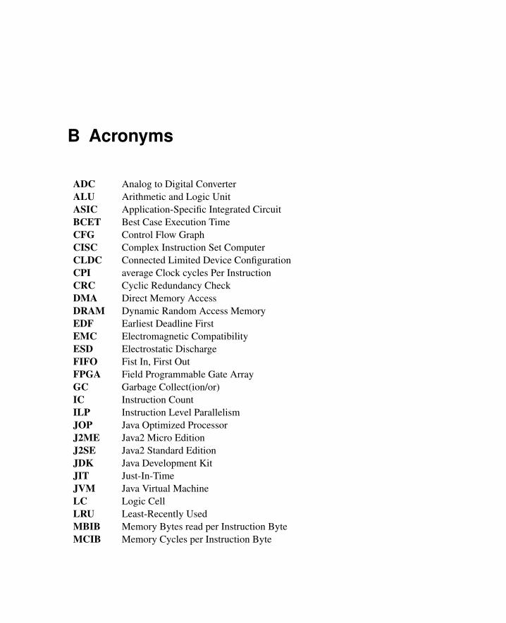
B Acronyms
ADC Analog to Digital ConverterALU Arithmetic and Logic UnitASIC Application-Specific Integrated CircuitBCET Best Case Execution TimeCFG Control Flow GraphCISC Complex Instruction Set ComputerCLDC Connected Limited Device ConfigurationCPI average Clock cycles Per InstructionCRC Cyclic Redundancy CheckDMA Direct Memory AccessDRAM Dynamic Random Access MemoryEDF Earliest Deadline FirstEMC Electromagnetic CompatibilityESD Electrostatic DischargeFIFO Fist In, First OutFPGA Field Programmable Gate ArrayGC Garbage Collect(ion/or)IC Instruction CountILP Instruction Level ParallelismJOP Java Optimized ProcessorJ2ME Java2 Micro EditionJ2SE Java2 Standard EditionJDK Java Development KitJIT Just-In-TimeJVM Java Virtual MachineLC Logic CellLRU Least-Recently UsedMBIB Memory Bytes read per Instruction ByteMCIB Memory Cycles per Instruction Byte
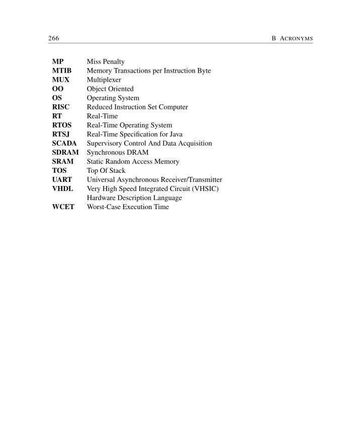
266 B ACRONYMS
MP Miss PenaltyMTIB Memory Transactions per Instruction ByteMUX MultiplexerOO Object OrientedOS Operating SystemRISC Reduced Instruction Set ComputerRT Real-TimeRTOS Real-Time Operating SystemRTSJ Real-Time Specification for JavaSCADA Supervisory Control And Data AcquisitionSDRAM Synchronous DRAMSRAM Static Random Access MemoryTOS Top Of StackUART Universal Asynchronous Receiver/TransmitterVHDL Very High Speed Integrated Circuit (VHSIC)
Hardware Description LanguageWCET Worst-Case Execution Time
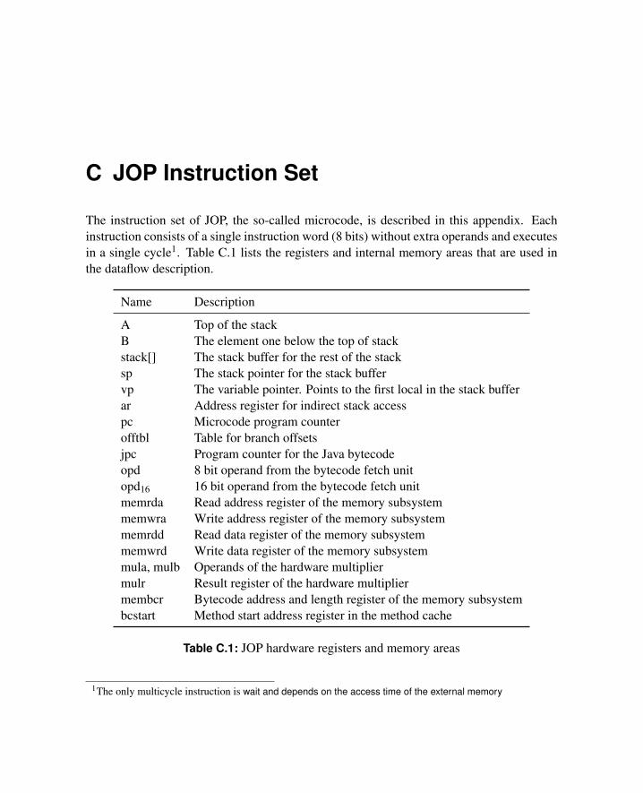
C JOP Instruction Set
The instruction set of JOP, the so-called microcode, is described in this appendix. Eachinstruction consists of a single instruction word (8 bits) without extra operands and executesin a single cycle1. Table C.1 lists the registers and internal memory areas that are used inthe dataflow description.
Name Description
A Top of the stackB The element one below the top of stackstack[] The stack buffer for the rest of the stacksp The stack pointer for the stack buffervp The variable pointer. Points to the first local in the stack bufferar Address register for indirect stack accesspc Microcode program counterofftbl Table for branch offsetsjpc Program counter for the Java bytecodeopd 8 bit operand from the bytecode fetch unitopd16 16 bit operand from the bytecode fetch unitmemrda Read address register of the memory subsystemmemwra Write address register of the memory subsystemmemrdd Read data register of the memory subsystemmemwrd Write data register of the memory subsystemmula, mulb Operands of the hardware multipliermulr Result register of the hardware multipliermembcr Bytecode address and length register of the memory subsystembcstart Method start address register in the method cache
Table C.1: JOP hardware registers and memory areas
1The only multicycle instruction is wait and depends on the access time of the external memory
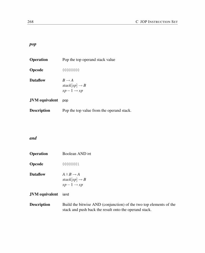
268 C JOP INSTRUCTION SET
pop
Operation Pop the top operand stack value
Opcode 00000000
Dataflow B→ Astack[sp]→ Bsp−1→ sp
JVM equivalent pop
Description Pop the top value from the operand stack.
and
Operation Boolean AND int
Opcode 00000001
Dataflow A∧B→ Astack[sp]→ Bsp−1→ sp
JVM equivalent iand
Description Build the bitwise AND (conjunction) of the two top elements of thestack and push back the result onto the operand stack.
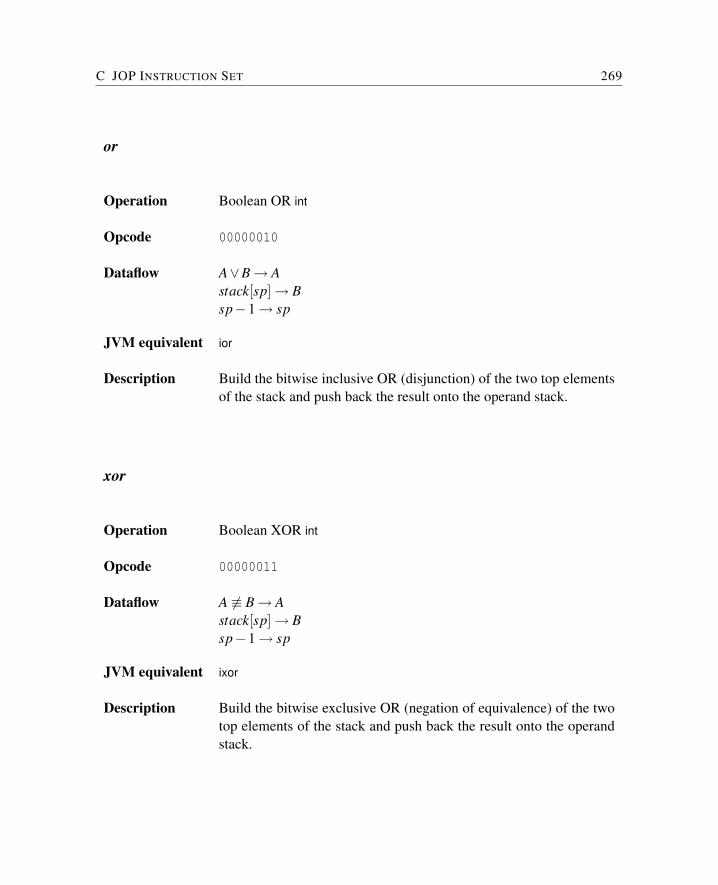
C JOP INSTRUCTION SET 269
or
Operation Boolean OR int
Opcode 00000010
Dataflow A∨B→ Astack[sp]→ Bsp−1→ sp
JVM equivalent ior
Description Build the bitwise inclusive OR (disjunction) of the two top elementsof the stack and push back the result onto the operand stack.
xor
Operation Boolean XOR int
Opcode 00000011
Dataflow A 6≡ B→ Astack[sp]→ Bsp−1→ sp
JVM equivalent ixor
Description Build the bitwise exclusive OR (negation of equivalence) of the twotop elements of the stack and push back the result onto the operandstack.
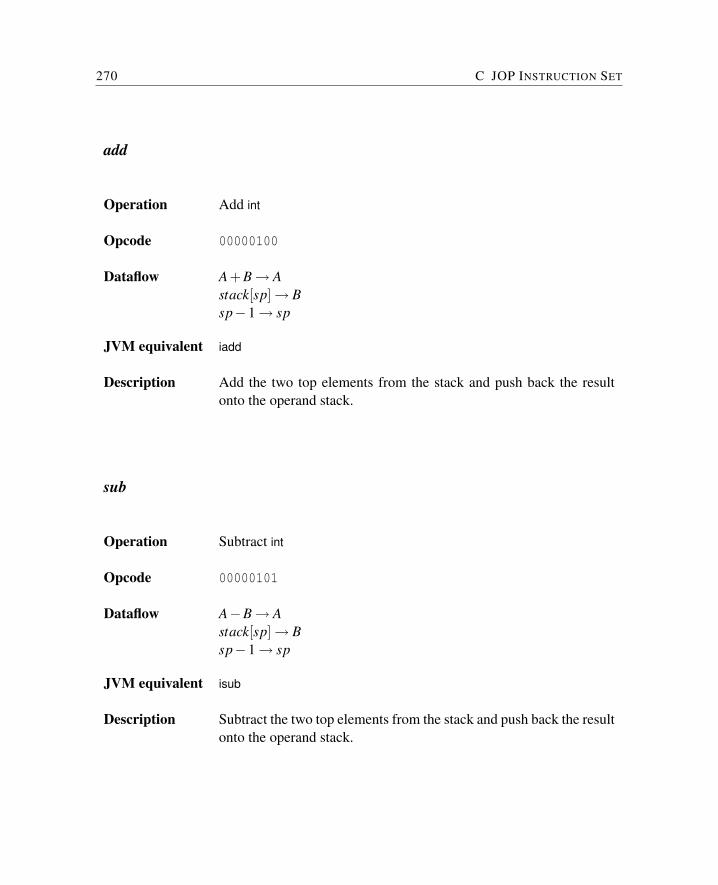
270 C JOP INSTRUCTION SET
add
Operation Add int
Opcode 00000100
Dataflow A+B→ Astack[sp]→ Bsp−1→ sp
JVM equivalent iadd
Description Add the two top elements from the stack and push back the resultonto the operand stack.
sub
Operation Subtract int
Opcode 00000101
Dataflow A−B→ Astack[sp]→ Bsp−1→ sp
JVM equivalent isub
Description Subtract the two top elements from the stack and push back the resultonto the operand stack.
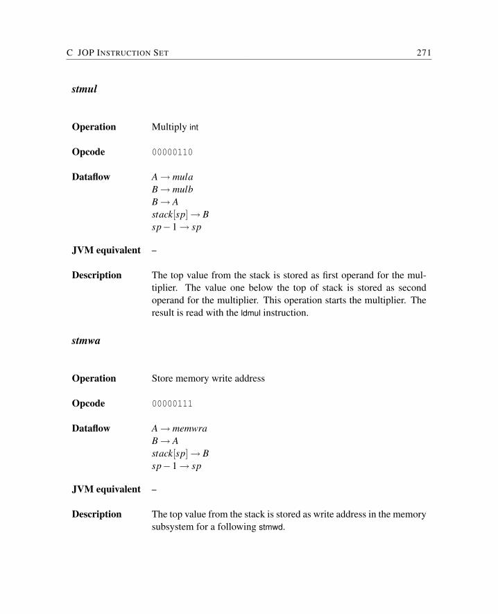
C JOP INSTRUCTION SET 271
stmul
Operation Multiply int
Opcode 00000110
Dataflow A→ mulaB→ mulbB→ Astack[sp]→ Bsp−1→ sp
JVM equivalent –
Description The top value from the stack is stored as first operand for the mul-tiplier. The value one below the top of stack is stored as secondoperand for the multiplier. This operation starts the multiplier. Theresult is read with the ldmul instruction.
stmwa
Operation Store memory write address
Opcode 00000111
Dataflow A→ memwraB→ Astack[sp]→ Bsp−1→ sp
JVM equivalent –
Description The top value from the stack is stored as write address in the memorysubsystem for a following stmwd.
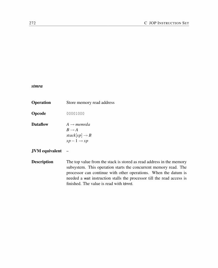
272 C JOP INSTRUCTION SET
stmra
Operation Store memory read address
Opcode 00001000
Dataflow A→ memrdaB→ Astack[sp]→ Bsp−1→ sp
JVM equivalent –
Description The top value from the stack is stored as read address in the memorysubsystem. This operation starts the concurrent memory read. Theprocessor can continue with other operations. When the datum isneeded a wait instruction stalls the processor till the read access isfinished. The value is read with ldmrd.
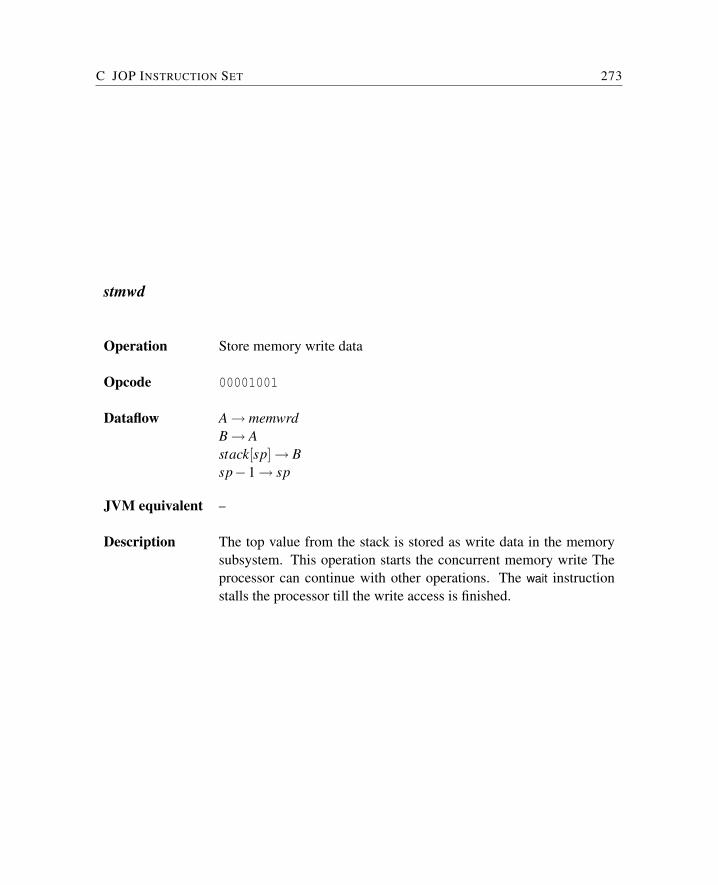
C JOP INSTRUCTION SET 273
stmwd
Operation Store memory write data
Opcode 00001001
Dataflow A→ memwrdB→ Astack[sp]→ Bsp−1→ sp
JVM equivalent –
Description The top value from the stack is stored as write data in the memorysubsystem. This operation starts the concurrent memory write Theprocessor can continue with other operations. The wait instructionstalls the processor till the write access is finished.
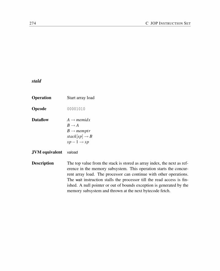
274 C JOP INSTRUCTION SET
stald
Operation Start array load
Opcode 00001010
Dataflow A→ memidxB→ AB→ memptrstack[sp]→ Bsp−1→ sp
JVM equivalent xaload
Description The top value from the stack is stored as array index, the next as ref-erence in the memory subsystem. This operation starts the concur-rent array load. The processor can continue with other operations.The wait instruction stalls the processor till the read access is fin-ished. A null pointer or out of bounds exception is generated by thememory subsystem and thrown at the next bytecode fetch.
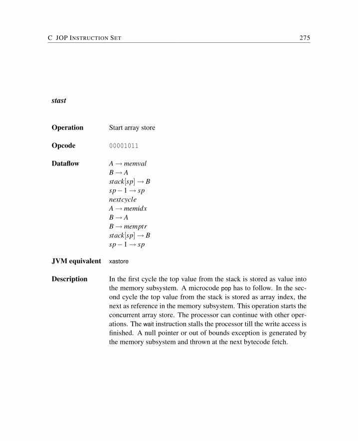
C JOP INSTRUCTION SET 275
stast
Operation Start array store
Opcode 00001011
Dataflow A→ memvalB→ Astack[sp]→ Bsp−1→ spnextcycleA→ memidxB→ AB→ memptrstack[sp]→ Bsp−1→ sp
JVM equivalent xastore
Description In the first cycle the top value from the stack is stored as value intothe memory subsystem. A microcode pop has to follow. In the sec-ond cycle the top value from the stack is stored as array index, thenext as reference in the memory subsystem. This operation starts theconcurrent array store. The processor can continue with other oper-ations. The wait instruction stalls the processor till the write access isfinished. A null pointer or out of bounds exception is generated bythe memory subsystem and thrown at the next bytecode fetch.
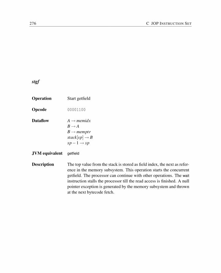
276 C JOP INSTRUCTION SET
stgf
Operation Start getfield
Opcode 00001100
Dataflow A→ memidxB→ AB→ memptrstack[sp]→ Bsp−1→ sp
JVM equivalent getfield
Description The top value from the stack is stored as field index, the next as refer-ence in the memory subsystem. This operation starts the concurrentgetfield. The processor can continue with other operations. The waitinstruction stalls the processor till the read access is finished. A nullpointer exception is generated by the memory subsystem and thrownat the next bytecode fetch.
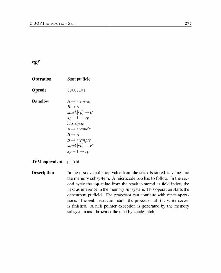
C JOP INSTRUCTION SET 277
stpf
Operation Start putfield
Opcode 00001101
Dataflow A→ memvalB→ Astack[sp]→ Bsp−1→ spnextcycleA→ memidxB→ AB→ memptrstack[sp]→ Bsp−1→ sp
JVM equivalent putfield
Description In the first cycle the top value from the stack is stored as value intothe memory subsystem. A microcode pop has to follow. In the sec-ond cycle the top value from the stack is stored as field index, thenext as reference in the memory subsystem. This operation starts theconcurrent putfield. The processor can continue with other opera-tions. The wait instruction stalls the processor till the write accessis finished. A null pointer exception is generated by the memorysubsystem and thrown at the next bytecode fetch.
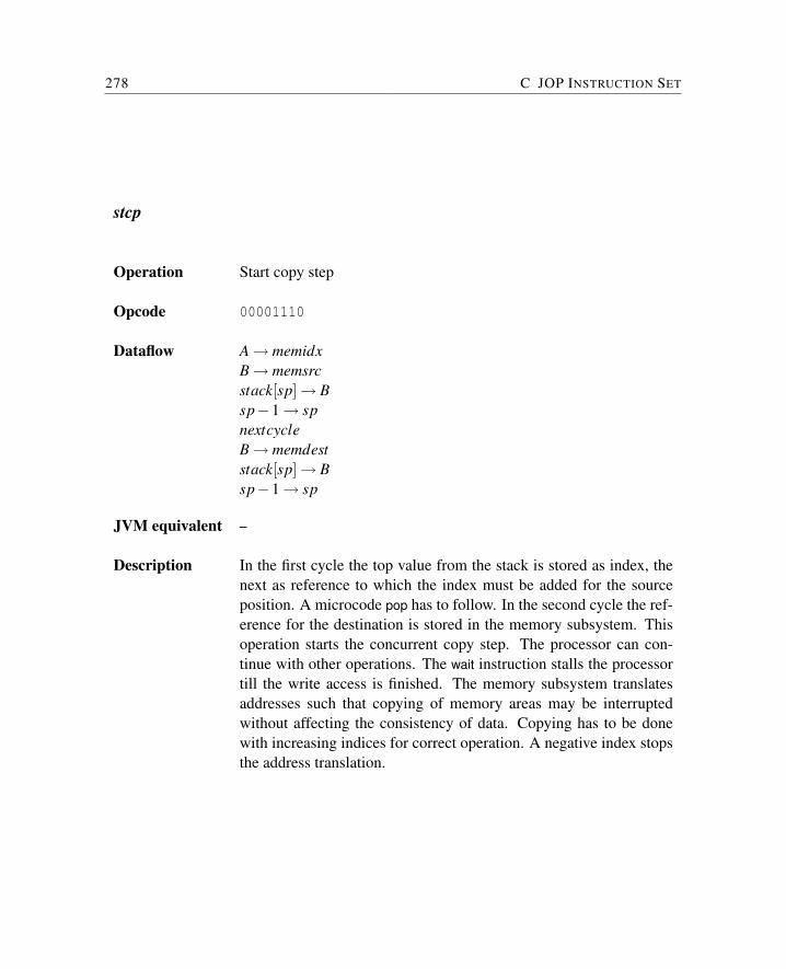
278 C JOP INSTRUCTION SET
stcp
Operation Start copy step
Opcode 00001110
Dataflow A→ memidxB→ memsrcstack[sp]→ Bsp−1→ spnextcycleB→ memdeststack[sp]→ Bsp−1→ sp
JVM equivalent –
Description In the first cycle the top value from the stack is stored as index, thenext as reference to which the index must be added for the sourceposition. A microcode pop has to follow. In the second cycle the ref-erence for the destination is stored in the memory subsystem. Thisoperation starts the concurrent copy step. The processor can con-tinue with other operations. The wait instruction stalls the processortill the write access is finished. The memory subsystem translatesaddresses such that copying of memory areas may be interruptedwithout affecting the consistency of data. Copying has to be donewith increasing indices for correct operation. A negative index stopsthe address translation.
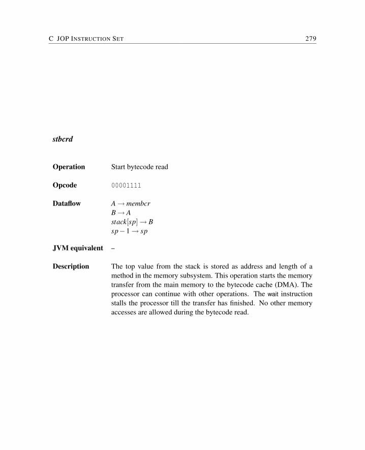
C JOP INSTRUCTION SET 279
stbcrd
Operation Start bytecode read
Opcode 00001111
Dataflow A→ membcrB→ Astack[sp]→ Bsp−1→ sp
JVM equivalent –
Description The top value from the stack is stored as address and length of amethod in the memory subsystem. This operation starts the memorytransfer from the main memory to the bytecode cache (DMA). Theprocessor can continue with other operations. The wait instructionstalls the processor till the transfer has finished. No other memoryaccesses are allowed during the bytecode read.
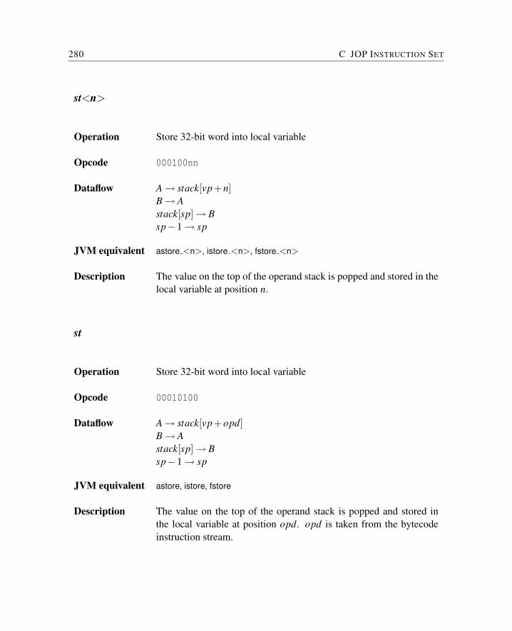
280 C JOP INSTRUCTION SET
st<n>
Operation Store 32-bit word into local variable
Opcode 000100nn
Dataflow A→ stack[vp+n]B→ Astack[sp]→ Bsp−1→ sp
JVM equivalent astore <n>, istore <n>, fstore <n>
Description The value on the top of the operand stack is popped and stored in thelocal variable at position n.
st
Operation Store 32-bit word into local variable
Opcode 00010100
Dataflow A→ stack[vp+opd]B→ Astack[sp]→ Bsp−1→ sp
JVM equivalent astore, istore, fstore
Description The value on the top of the operand stack is popped and stored inthe local variable at position opd. opd is taken from the bytecodeinstruction stream.
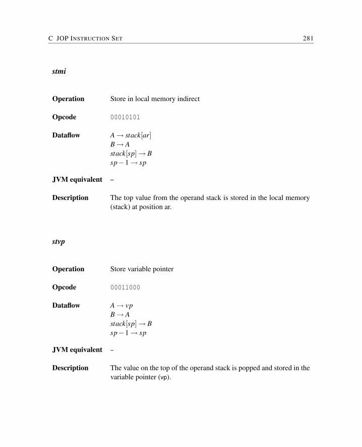
C JOP INSTRUCTION SET 281
stmi
Operation Store in local memory indirect
Opcode 00010101
Dataflow A→ stack[ar]B→ Astack[sp]→ Bsp−1→ sp
JVM equivalent –
Description The top value from the operand stack is stored in the local memory(stack) at position ar.
stvp
Operation Store variable pointer
Opcode 00011000
Dataflow A→ vpB→ Astack[sp]→ Bsp−1→ sp
JVM equivalent –
Description The value on the top of the operand stack is popped and stored in thevariable pointer (vp).
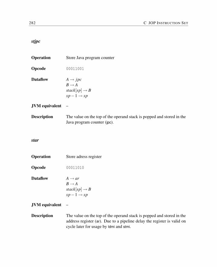
282 C JOP INSTRUCTION SET
stjpc
Operation Store Java program counter
Opcode 00011001
Dataflow A→ jpcB→ Astack[sp]→ Bsp−1→ sp
JVM equivalent –
Description The value on the top of the operand stack is popped and stored in theJava program counter (jpc).
star
Operation Store adress register
Opcode 00011010
Dataflow A→ arB→ Astack[sp]→ Bsp−1→ sp
JVM equivalent –
Description The value on the top of the operand stack is popped and stored in theaddress register (ar). Due to a pipeline delay the register is valid oncycle later for usage by ldmi and stmi.
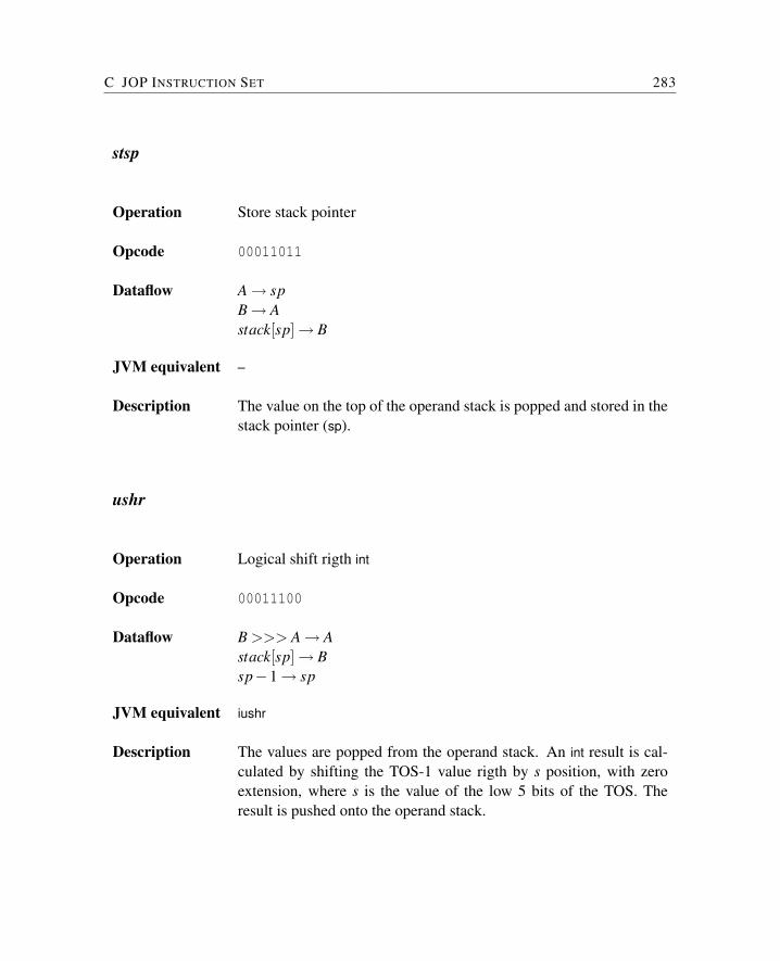
C JOP INSTRUCTION SET 283
stsp
Operation Store stack pointer
Opcode 00011011
Dataflow A→ spB→ Astack[sp]→ B
JVM equivalent –
Description The value on the top of the operand stack is popped and stored in thestack pointer (sp).
ushr
Operation Logical shift rigth int
Opcode 00011100
Dataflow B >>> A→ Astack[sp]→ Bsp−1→ sp
JVM equivalent iushr
Description The values are popped from the operand stack. An int result is cal-culated by shifting the TOS-1 value rigth by s position, with zeroextension, where s is the value of the low 5 bits of the TOS. Theresult is pushed onto the operand stack.
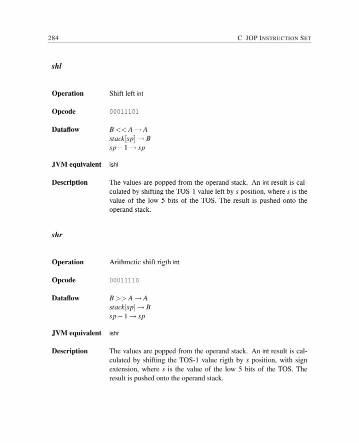
284 C JOP INSTRUCTION SET
shl
Operation Shift left int
Opcode 00011101
Dataflow B << A→ Astack[sp]→ Bsp−1→ sp
JVM equivalent ishl
Description The values are popped from the operand stack. An int result is cal-culated by shifting the TOS-1 value left by s position, where s is thevalue of the low 5 bits of the TOS. The result is pushed onto theoperand stack.
shr
Operation Arithmetic shift rigth int
Opcode 00011110
Dataflow B >> A→ Astack[sp]→ Bsp−1→ sp
JVM equivalent ishr
Description The values are popped from the operand stack. An int result is cal-culated by shifting the TOS-1 value rigth by s position, with signextension, where s is the value of the low 5 bits of the TOS. Theresult is pushed onto the operand stack.
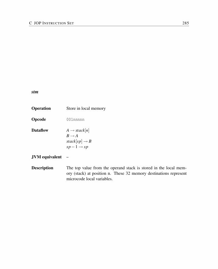
C JOP INSTRUCTION SET 285
stm
Operation Store in local memory
Opcode 001nnnnn
Dataflow A→ stack[n]B→ Astack[sp]→ Bsp−1→ sp
JVM equivalent –
Description The top value from the operand stack is stored in the local mem-ory (stack) at position n. These 32 memory destinations representmicrocode local variables.
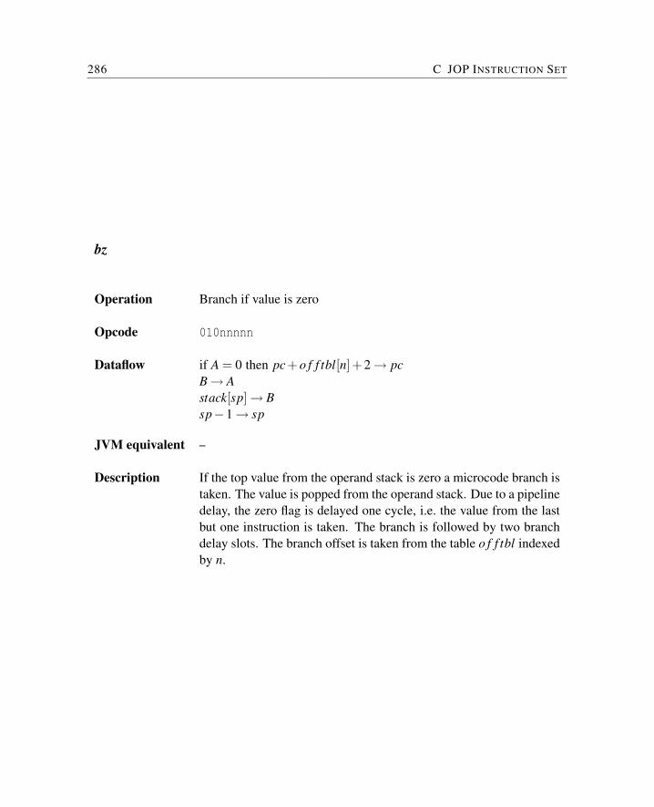
286 C JOP INSTRUCTION SET
bz
Operation Branch if value is zero
Opcode 010nnnnn
Dataflow if A = 0 then pc+o f f tbl[n]+2→ pcB→ Astack[sp]→ Bsp−1→ sp
JVM equivalent –
Description If the top value from the operand stack is zero a microcode branch istaken. The value is popped from the operand stack. Due to a pipelinedelay, the zero flag is delayed one cycle, i.e. the value from the lastbut one instruction is taken. The branch is followed by two branchdelay slots. The branch offset is taken from the table o f f tbl indexedby n.
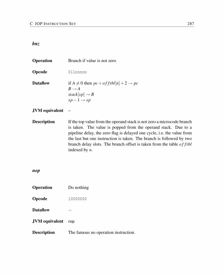
C JOP INSTRUCTION SET 287
bnz
Operation Branch if value is not zero
Opcode 011nnnnn
Dataflow if A 6= 0 then pc+o f f tbl[n]+2→ pcB→ Astack[sp]→ Bsp−1→ sp
JVM equivalent –
Description If the top value from the operand stack is not zero a microcode branchis taken. The value is popped from the operand stack. Due to apipeline delay, the zero flag is delayed one cycle, i.e. the value fromthe last but one instruction is taken. The branch is followed by twobranch delay slots. The branch offset is taken from the table o f f tblindexed by n.
nop
Operation Do nothing
Opcode 10000000
Dataflow −
JVM equivalent nop
Description The famous no operation instruction.
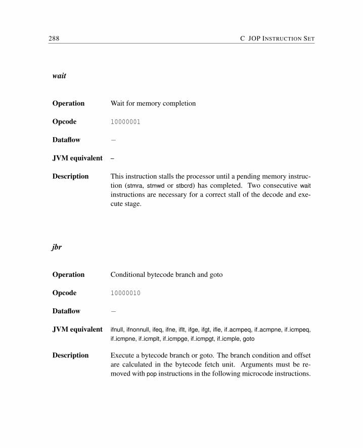
288 C JOP INSTRUCTION SET
wait
Operation Wait for memory completion
Opcode 10000001
Dataflow −
JVM equivalent –
Description This instruction stalls the processor until a pending memory instruc-tion (stmra, stmwd or stbcrd) has completed. Two consecutive waitinstructions are necessary for a correct stall of the decode and exe-cute stage.
jbr
Operation Conditional bytecode branch and goto
Opcode 10000010
Dataflow −
JVM equivalent ifnull, ifnonnull, ifeq, ifne, iflt, ifge, ifgt, ifle, if acmpeq, if acmpne, if icmpeq,if icmpne, if icmplt, if icmpge, if icmpgt, if icmple, goto
Description Execute a bytecode branch or goto. The branch condition and offsetare calculated in the bytecode fetch unit. Arguments must be re-moved with pop instructions in the following microcode instructions.
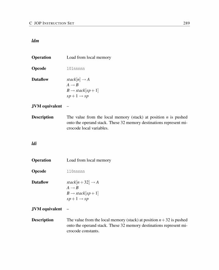
C JOP INSTRUCTION SET 289
ldm
Operation Load from local memory
Opcode 101nnnnn
Dataflow stack[n]→ AA→ BB→ stack[sp+1]sp+1→ sp
JVM equivalent –
Description The value from the local memory (stack) at position n is pushedonto the operand stack. These 32 memory destinations represent mi-crocode local variables.
ldi
Operation Load from local memory
Opcode 110nnnnn
Dataflow stack[n+32]→ AA→ BB→ stack[sp+1]sp+1→ sp
JVM equivalent –
Description The value from the local memory (stack) at position n+32 is pushedonto the operand stack. These 32 memory destinations represent mi-crocode constants.
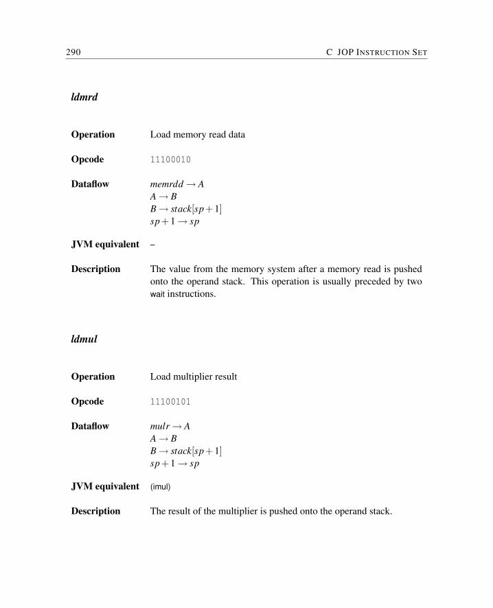
290 C JOP INSTRUCTION SET
ldmrd
Operation Load memory read data
Opcode 11100010
Dataflow memrdd→ AA→ BB→ stack[sp+1]sp+1→ sp
JVM equivalent –
Description The value from the memory system after a memory read is pushedonto the operand stack. This operation is usually preceded by twowait instructions.
ldmul
Operation Load multiplier result
Opcode 11100101
Dataflow mulr→ AA→ BB→ stack[sp+1]sp+1→ sp
JVM equivalent (imul)
Description The result of the multiplier is pushed onto the operand stack.
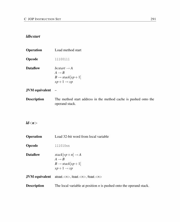
C JOP INSTRUCTION SET 291
ldbcstart
Operation Load method start
Opcode 11100111
Dataflow bcstart→ AA→ BB→ stack[sp+1]sp+1→ sp
JVM equivalent –
Description The method start address in the method cache is pushed onto theoperand stack.
ld<n>
Operation Load 32-bit word from local variable
Opcode 111010nn
Dataflow stack[vp+n]→ AA→ BB→ stack[sp+1]sp+1→ sp
JVM equivalent aload <n>, iload <n>, fload <n>
Description The local variable at position n is pushed onto the operand stack.
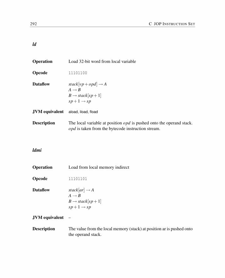
292 C JOP INSTRUCTION SET
ld
Operation Load 32-bit word from local variable
Opcode 11101100
Dataflow stack[vp+opd]→ AA→ BB→ stack[sp+1]sp+1→ sp
JVM equivalent aload, iload, fload
Description The local variable at position opd is pushed onto the operand stack.opd is taken from the bytecode instruction stream.
ldmi
Operation Load from local memory indirect
Opcode 11101101
Dataflow stack[ar]→ AA→ BB→ stack[sp+1]sp+1→ sp
JVM equivalent –
Description The value from the local memory (stack) at position ar is pushed ontothe operand stack.
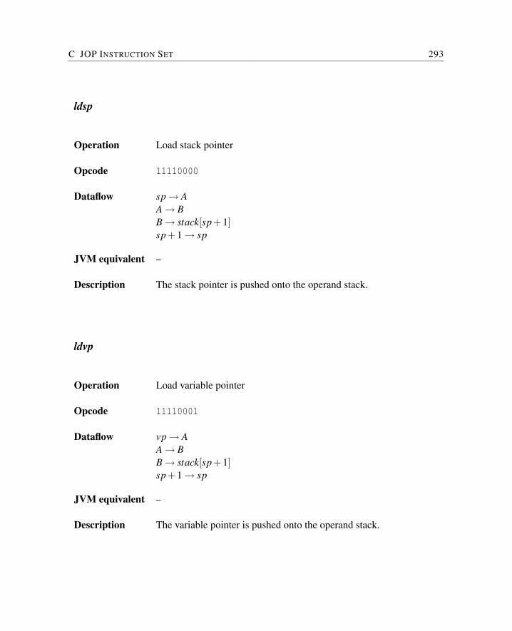
C JOP INSTRUCTION SET 293
ldsp
Operation Load stack pointer
Opcode 11110000
Dataflow sp→ AA→ BB→ stack[sp+1]sp+1→ sp
JVM equivalent –
Description The stack pointer is pushed onto the operand stack.
ldvp
Operation Load variable pointer
Opcode 11110001
Dataflow vp→ AA→ BB→ stack[sp+1]sp+1→ sp
JVM equivalent –
Description The variable pointer is pushed onto the operand stack.
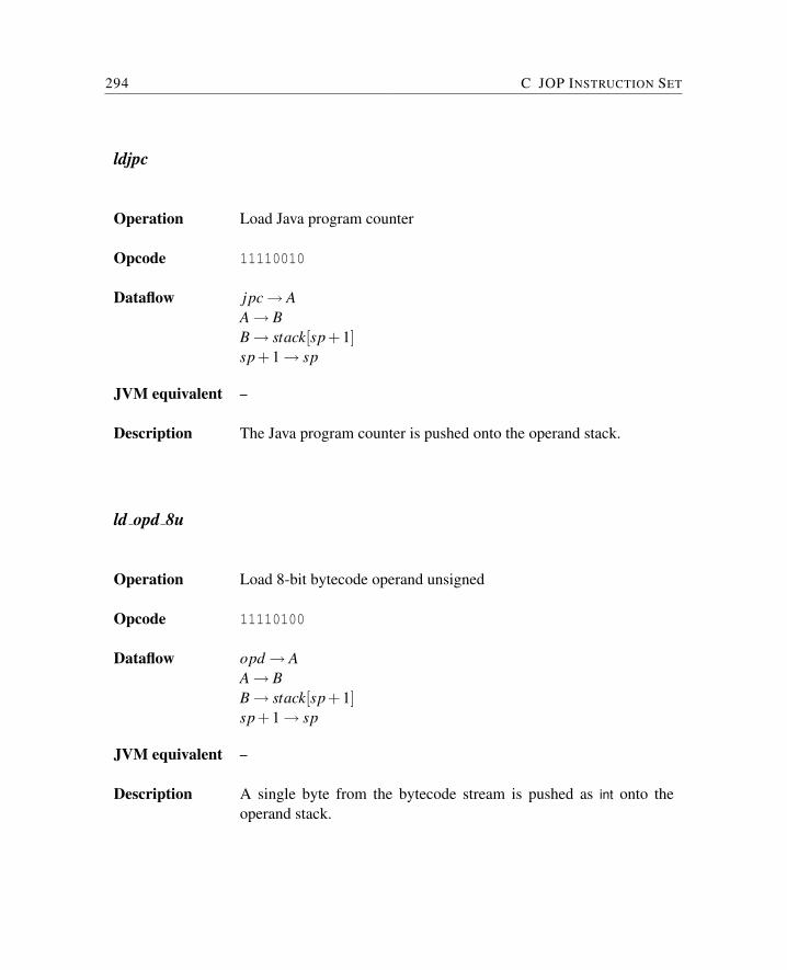
294 C JOP INSTRUCTION SET
ldjpc
Operation Load Java program counter
Opcode 11110010
Dataflow jpc→ AA→ BB→ stack[sp+1]sp+1→ sp
JVM equivalent –
Description The Java program counter is pushed onto the operand stack.
ld opd 8u
Operation Load 8-bit bytecode operand unsigned
Opcode 11110100
Dataflow opd→ AA→ BB→ stack[sp+1]sp+1→ sp
JVM equivalent –
Description A single byte from the bytecode stream is pushed as int onto theoperand stack.
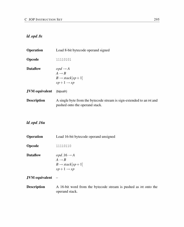
C JOP INSTRUCTION SET 295
ld opd 8s
Operation Load 8-bit bytecode operand signed
Opcode 11110101
Dataflow opd→ AA→ BB→ stack[sp+1]sp+1→ sp
JVM equivalent (bipush)
Description A single byte from the bytecode stream is sign-extended to an int andpushed onto the operand stack.
ld opd 16u
Operation Load 16-bit bytecode operand unsigned
Opcode 11110110
Dataflow opd 16→ AA→ BB→ stack[sp+1]sp+1→ sp
JVM equivalent –
Description A 16-bit word from the bytecode stream is pushed as int onto theoperand stack.
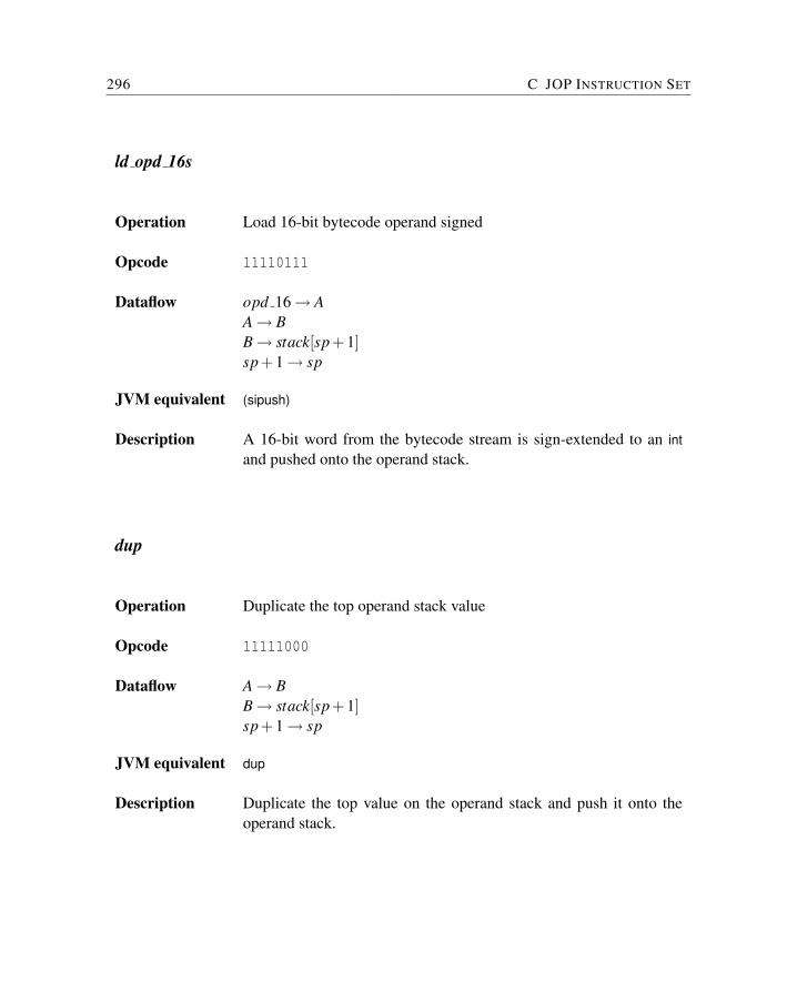
296 C JOP INSTRUCTION SET
ld opd 16s
Operation Load 16-bit bytecode operand signed
Opcode 11110111
Dataflow opd 16→ AA→ BB→ stack[sp+1]sp+1→ sp
JVM equivalent (sipush)
Description A 16-bit word from the bytecode stream is sign-extended to an intand pushed onto the operand stack.
dup
Operation Duplicate the top operand stack value
Opcode 11111000
Dataflow A→ BB→ stack[sp+1]sp+1→ sp
JVM equivalent dup
Description Duplicate the top value on the operand stack and push it onto theoperand stack.
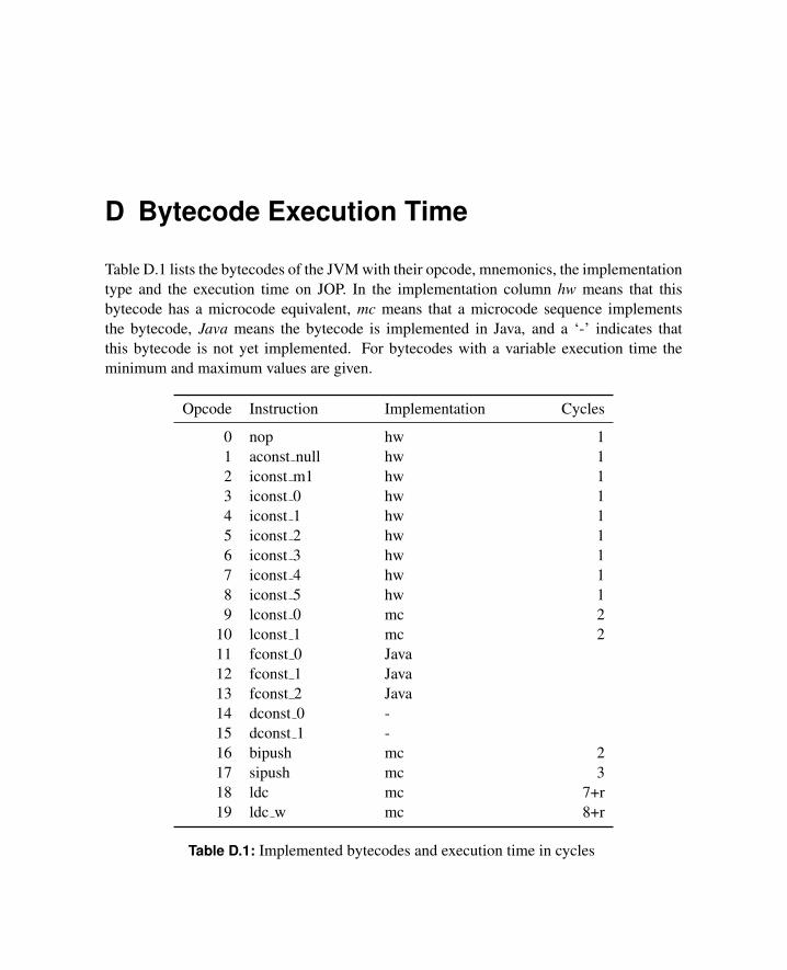
D Bytecode Execution Time
Table D.1 lists the bytecodes of the JVM with their opcode, mnemonics, the implementationtype and the execution time on JOP. In the implementation column hw means that thisbytecode has a microcode equivalent, mc means that a microcode sequence implementsthe bytecode, Java means the bytecode is implemented in Java, and a ‘-’ indicates thatthis bytecode is not yet implemented. For bytecodes with a variable execution time theminimum and maximum values are given.
Opcode Instruction Implementation Cycles
0 nop hw 11 aconst null hw 12 iconst m1 hw 13 iconst 0 hw 14 iconst 1 hw 15 iconst 2 hw 16 iconst 3 hw 17 iconst 4 hw 18 iconst 5 hw 19 lconst 0 mc 2
10 lconst 1 mc 211 fconst 0 Java12 fconst 1 Java13 fconst 2 Java14 dconst 0 -15 dconst 1 -16 bipush mc 217 sipush mc 318 ldc mc 7+r19 ldc w mc 8+r
Table D.1: Implemented bytecodes and execution time in cycles
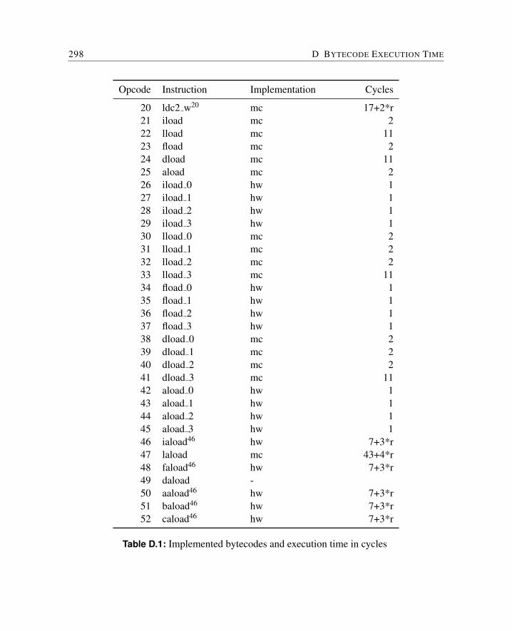
298 D BYTECODE EXECUTION TIME
Opcode Instruction Implementation Cycles
20 ldc2 w20 mc 17+2*r21 iload mc 222 lload mc 1123 fload mc 224 dload mc 1125 aload mc 226 iload 0 hw 127 iload 1 hw 128 iload 2 hw 129 iload 3 hw 130 lload 0 mc 231 lload 1 mc 232 lload 2 mc 233 lload 3 mc 1134 fload 0 hw 135 fload 1 hw 136 fload 2 hw 137 fload 3 hw 138 dload 0 mc 239 dload 1 mc 240 dload 2 mc 241 dload 3 mc 1142 aload 0 hw 143 aload 1 hw 144 aload 2 hw 145 aload 3 hw 146 iaload46 hw 7+3*r47 laload mc 43+4*r48 faload46 hw 7+3*r49 daload -50 aaload46 hw 7+3*r51 baload46 hw 7+3*r52 caload46 hw 7+3*r
Table D.1: Implemented bytecodes and execution time in cycles
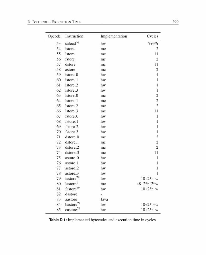
D BYTECODE EXECUTION TIME 299
Opcode Instruction Implementation Cycles
53 saload46 hw 7+3*r54 istore mc 255 lstore mc 1156 fstore mc 257 dstore mc 1158 astore mc 259 istore 0 hw 160 istore 1 hw 161 istore 2 hw 162 istore 3 hw 163 lstore 0 mc 264 lstore 1 mc 265 lstore 2 mc 266 lstore 3 mc 1167 fstore 0 hw 168 fstore 1 hw 169 fstore 2 hw 170 fstore 3 hw 171 dstore 0 mc 272 dstore 1 mc 273 dstore 2 mc 274 dstore 3 mc 1175 astore 0 hw 176 astore 1 hw 177 astore 2 hw 178 astore 3 hw 179 iastore79 hw 10+2*r+w80 lastore1 mc 48+2*r+2*w81 fastore79 hw 10+2*r+w82 dastore -83 aastore Java84 bastore79 hw 10+2*r+w85 castore79 hw 10+2*r+w
Table D.1: Implemented bytecodes and execution time in cycles
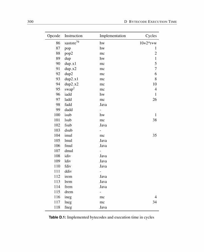
300 D BYTECODE EXECUTION TIME
Opcode Instruction Implementation Cycles
86 sastore79 hw 10+2*r+w87 pop hw 188 pop2 mc 289 dup hw 190 dup x1 mc 591 dup x2 mc 792 dup2 mc 693 dup2 x1 mc 894 dup2 x2 mc 1095 swap2 mc 496 iadd hw 197 ladd mc 2698 fadd Java99 dadd -
100 isub hw 1101 lsub mc 38102 fsub Java103 dsub -104 imul mc 35105 lmul Java106 fmul Java107 dmul -108 idiv Java109 ldiv Java110 fdiv Java111 ddiv -112 irem Java113 lrem Java114 frem Java115 drem -116 ineg mc 4117 lneg mc 34118 fneg Java
Table D.1: Implemented bytecodes and execution time in cycles
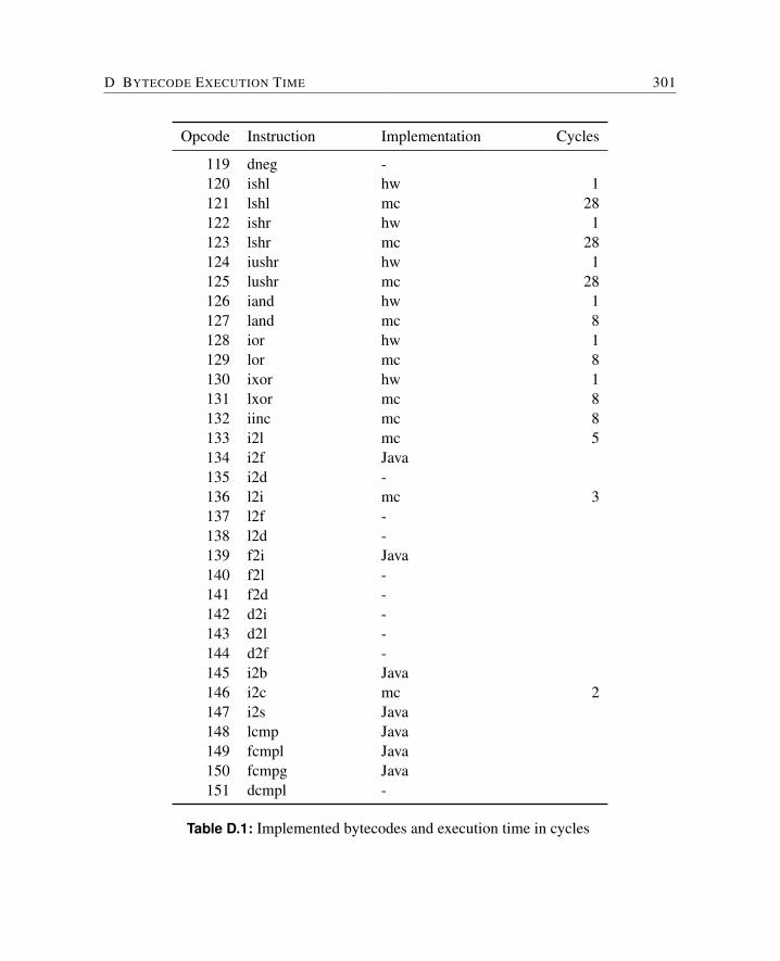
D BYTECODE EXECUTION TIME 301
Opcode Instruction Implementation Cycles
119 dneg -120 ishl hw 1121 lshl mc 28122 ishr hw 1123 lshr mc 28124 iushr hw 1125 lushr mc 28126 iand hw 1127 land mc 8128 ior hw 1129 lor mc 8130 ixor hw 1131 lxor mc 8132 iinc mc 8133 i2l mc 5134 i2f Java135 i2d -136 l2i mc 3137 l2f -138 l2d -139 f2i Java140 f2l -141 f2d -142 d2i -143 d2l -144 d2f -145 i2b Java146 i2c mc 2147 i2s Java148 lcmp Java149 fcmpl Java150 fcmpg Java151 dcmpl -
Table D.1: Implemented bytecodes and execution time in cycles
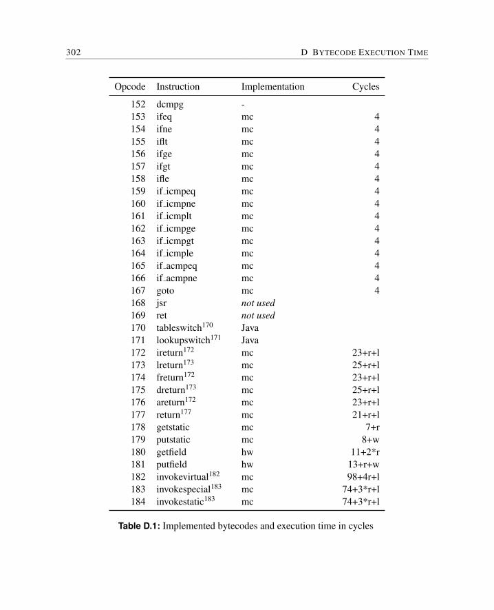
302 D BYTECODE EXECUTION TIME
Opcode Instruction Implementation Cycles
152 dcmpg -153 ifeq mc 4154 ifne mc 4155 iflt mc 4156 ifge mc 4157 ifgt mc 4158 ifle mc 4159 if icmpeq mc 4160 if icmpne mc 4161 if icmplt mc 4162 if icmpge mc 4163 if icmpgt mc 4164 if icmple mc 4165 if acmpeq mc 4166 if acmpne mc 4167 goto mc 4168 jsr not used169 ret not used170 tableswitch170 Java171 lookupswitch171 Java172 ireturn172 mc 23+r+l173 lreturn173 mc 25+r+l174 freturn172 mc 23+r+l175 dreturn173 mc 25+r+l176 areturn172 mc 23+r+l177 return177 mc 21+r+l178 getstatic mc 7+r179 putstatic mc 8+w180 getfield hw 11+2*r181 putfield hw 13+r+w182 invokevirtual182 mc 98+4r+l183 invokespecial183 mc 74+3*r+l184 invokestatic183 mc 74+3*r+l
Table D.1: Implemented bytecodes and execution time in cycles
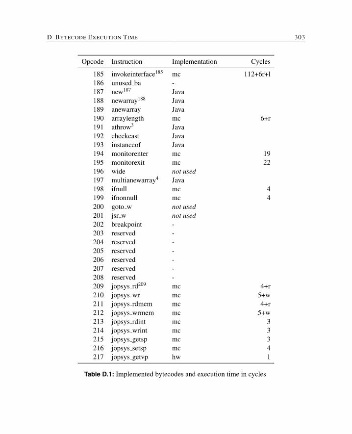
D BYTECODE EXECUTION TIME 303
Opcode Instruction Implementation Cycles
185 invokeinterface185 mc 112+6r+l186 unused ba -187 new187 Java188 newarray188 Java189 anewarray Java190 arraylength mc 6+r191 athrow3 Java192 checkcast Java193 instanceof Java194 monitorenter mc 19195 monitorexit mc 22196 wide not used197 multianewarray4 Java198 ifnull mc 4199 ifnonnull mc 4200 goto w not used201 jsr w not used202 breakpoint -203 reserved -204 reserved -205 reserved -206 reserved -207 reserved -208 reserved -209 jopsys rd209 mc 4+r210 jopsys wr mc 5+w211 jopsys rdmem mc 4+r212 jopsys wrmem mc 5+w213 jopsys rdint mc 3214 jopsys wrint mc 3215 jopsys getsp mc 3216 jopsys setsp mc 4217 jopsys getvp hw 1
Table D.1: Implemented bytecodes and execution time in cycles
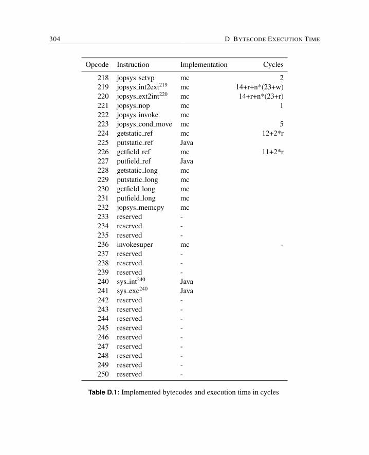
304 D BYTECODE EXECUTION TIME
Opcode Instruction Implementation Cycles
218 jopsys setvp mc 2219 jopsys int2ext219 mc 14+r+n*(23+w)220 jopsys ext2int220 mc 14+r+n*(23+r)221 jopsys nop mc 1222 jopsys invoke mc223 jopsys cond move mc 5224 getstatic ref mc 12+2*r225 putstatic ref Java226 getfield ref mc 11+2*r227 putfield ref Java228 getstatic long mc229 putstatic long mc230 getfield long mc231 putfield long mc232 jopsys memcpy mc233 reserved -234 reserved -235 reserved -236 invokesuper mc -237 reserved -238 reserved -239 reserved -240 sys int240 Java241 sys exc240 Java242 reserved -243 reserved -244 reserved -245 reserved -246 reserved -247 reserved -248 reserved -249 reserved -250 reserved -
Table D.1: Implemented bytecodes and execution time in cycles
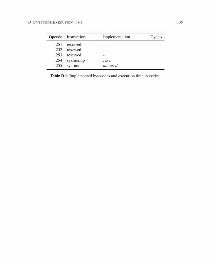
D BYTECODE EXECUTION TIME 305
Opcode Instruction Implementation Cycles
251 reserved -252 reserved -253 reserved -254 sys noimp Java255 sys init not used
Table D.1: Implemented bytecodes and execution time in cycles
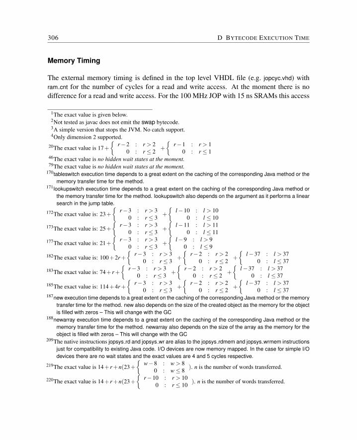
306 D BYTECODE EXECUTION TIME
Memory Timing
The external memory timing is defined in the top level VHDL file (e.g. jopcyc.vhd) withram cnt for the number of cycles for a read and write access. At the moment there is nodifference for a read and write access. For the 100 MHz JOP with 15 ns SRAMs this access
1The exact value is given below.2Not tested as javac does not emit the swap bytecode.3A simple version that stops the JVM. No catch support.4Only dimension 2 supported.
20The exact value is 17+{
r−2 : r > 20 : r ≤ 2
+{
r−1 : r > 10 : r ≤ 1
46The exact value is no hidden wait states at the moment.79The exact value is no hidden wait states at the moment.
170tableswitch execution time depends to a great extent on the caching of the corresponding Java method or thememory transfer time for the method.
171lookupswitch execution time depends to a great extent on the caching of the corresponding Java method orthe memory transfer time for the method. lookupswitch also depends on the argument as it performs a linearsearch in the jump table.
172The exact value is: 23+{
r−3 : r > 30 : r ≤ 3
+{
l−10 : l > 100 : l ≤ 10
173The exact value is: 25+{
r−3 : r > 30 : r ≤ 3
+{
l−11 : l > 110 : l ≤ 11
177The exact value is: 21+{
r−3 : r > 30 : r ≤ 3
+{
l−9 : l > 90 : l ≤ 9
182The exact value is: 100+2r +{
r−3 : r > 30 : r ≤ 3
+{
r−2 : r > 20 : r ≤ 2
+{
l−37 : l > 370 : l ≤ 37
183The exact value is: 74+ r +{
r−3 : r > 30 : r ≤ 3
+{
r−2 : r > 20 : r ≤ 2
+{
l−37 : l > 370 : l ≤ 37
185The exact value is: 114+4r +{
r−3 : r > 30 : r ≤ 3
+{
r−2 : r > 20 : r ≤ 2
+{
l−37 : l > 370 : l ≤ 37
187new execution time depends to a great extent on the caching of the corresponding Java method or the memorytransfer time for the method. new also depends on the size of the created object as the memory for the objectis filled with zeros – This will change with the GC
188newarray execution time depends to a great extent on the caching of the corresponding Java method or thememory transfer time for the method. newarray also depends on the size of the array as the memory for theobject is filled with zeros – This will change with the GC
209The native instructions jopsys rd and jopsys wr are alias to the jopsys rdmem and jopsys wrmem instructionsjust for compatibility to existing Java code. I/O devices are now memory mapped. In the case for simple I/Odevices there are no wait states and the exact values are 4 and 5 cycles respective.
219The exact value is 14+ r +n(23+{
w−8 : w > 80 : w≤ 8
). n is the number of words transferred.
220The exact value is 14+ r +n(23+{
r−10 : r > 100 : r ≤ 10
). n is the number of words transferred.
D BYTECODE EXECUTION TIME 307
time is two cycles (ram cnt=2, 20 ns). Therefore the wait state nws is 1 (ram cnt-1). A basicmemory read in microcode is as follows:
stmra // start read with address storewait // fill the pipeline with twowait // wait instructionsldmrd // push read result on TOS
In this sequence the last wait executes for 1+nws cycles. Therefore the whole read sequencetakes 4+nws cycles. For the example with ram cnt=2 this basic memory read takes 5 cycles.
A memory write in microcode is as follows:
stmwa // store addressstmwd // store data and start the writewait // fill the pipeline with waitwait // wait for the memory ready
The last wait again executes for 1+nws cycles and the basic write takes 4+nws cycles. Forthe native bytecode jopsys wrmem an additional nop instruction for the nxt flag is necessary.
The read and write wait states rws and wws are:
rws = wws ={
ram cnt−1 : ram cnt > 10 : ram cnt ≤ 1
In the instruction timing we use r and w instead of rws and wws. The wait states can behidden by other microcode instructions between stmra/wait and stmwd/wait. The exact valueis given in the footnote.
Instruction Timing
The bytecodes that access memory are indicated by an r for a memory read and an w fora memory write at the cycles column (r and w are the additional wait states). The waitcycles for the memory access have to be added to the execution time. These two values areimplementation dependent (clock frequency versus RAM access time, data bus width); forthe Cyclone EP1C6 board with 15 ns SRAMs and 100 MHz clock frequency these valuesare both 1 cycle (ram cnt-1).
For some bytecodes, part of the memory latency can be hidden by executing microcodeduring the memory access. However, these cycles can only be subtracted when the waitstates (r or w) are larger then 0 cycles. The exact execution time with the subtraction of thesaved cycles is given in the footnote.
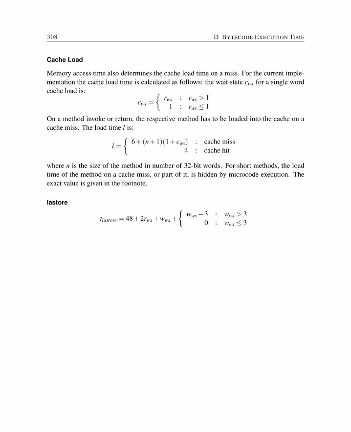
308 D BYTECODE EXECUTION TIME
Cache Load
Memory access time also determines the cache load time on a miss. For the current imple-mentation the cache load time is calculated as follows: the wait state cws for a single wordcache load is:
cws ={
rws : rws > 11 : rws ≤ 1
On a method invoke or return, the respective method has to be loaded into the cache on acache miss. The load time l is:
l ={
6+(n+1)(1+ cws) : cache miss4 : cache hit
where n is the size of the method in number of 32-bit words. For short methods, the loadtime of the method on a cache miss, or part of it, is hidden by microcode execution. Theexact value is given in the footnote.
lastore
tlastore = 48+2rws +wws +{
wws−3 : wws > 30 : wws ≤ 3
E Printed Circuit Boards
This chapter provides the schematics of the Cycore FPGA boards and several I/O extensionboards.
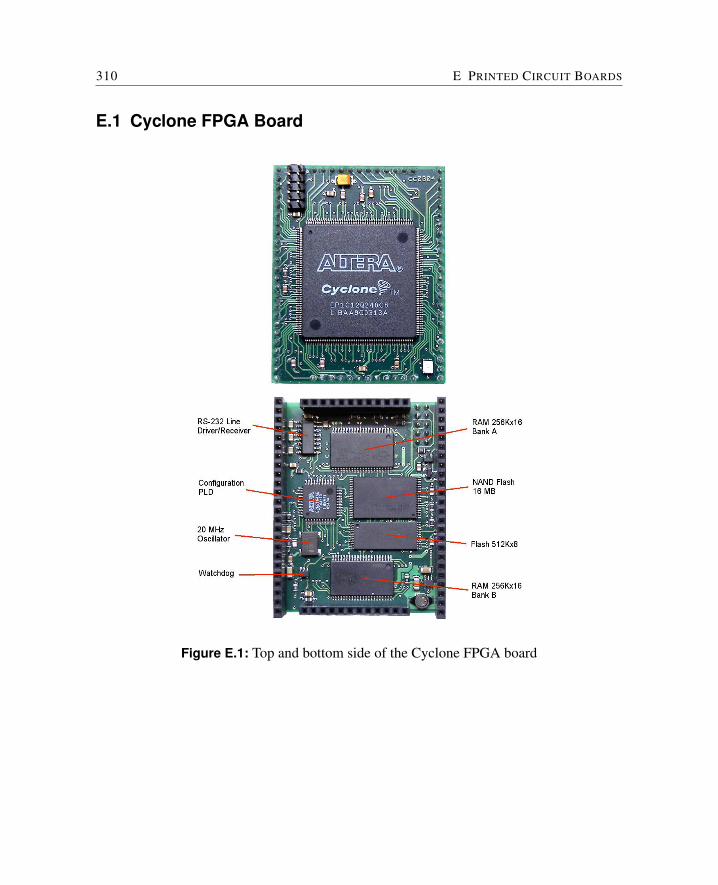
310 E PRINTED CIRCUIT BOARDS
E.1 Cyclone FPGA Board
Figure E.1: Top and bottom side of the Cyclone FPGA board
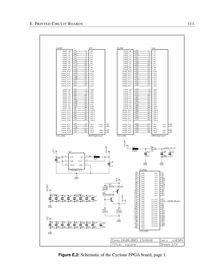
E PRINTED CIRCUIT BOARDS 311
Figure E.2: Schematic of the Cyclone FPGA board, page 1
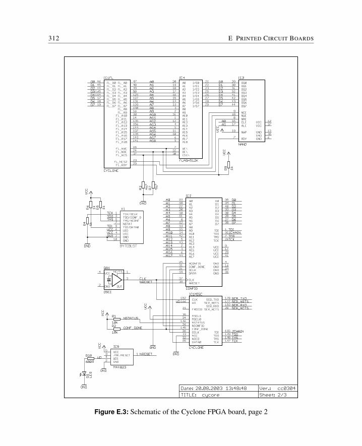
312 E PRINTED CIRCUIT BOARDS
Figure E.3: Schematic of the Cyclone FPGA board, page 2
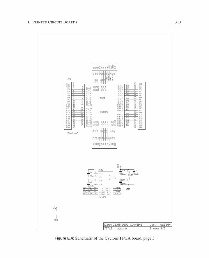
E PRINTED CIRCUIT BOARDS 313
Figure E.4: Schematic of the Cyclone FPGA board, page 3
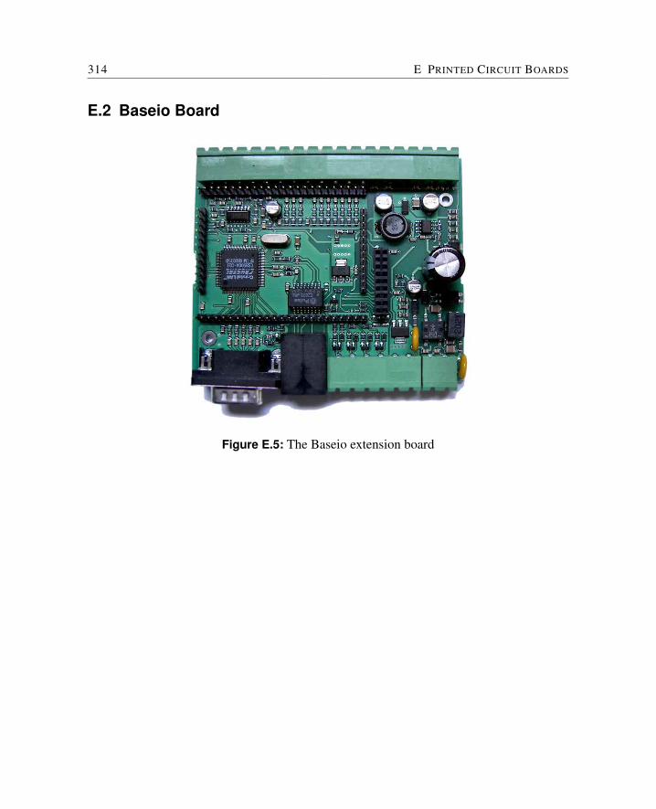
314 E PRINTED CIRCUIT BOARDS
E.2 Baseio Board
Figure E.5: The Baseio extension board
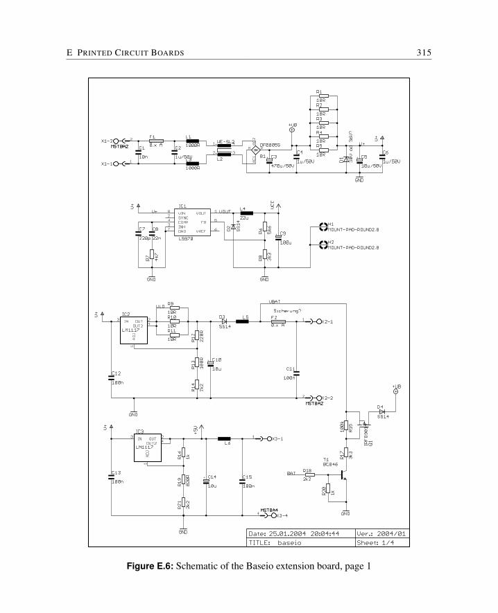
E PRINTED CIRCUIT BOARDS 315
Figure E.6: Schematic of the Baseio extension board, page 1
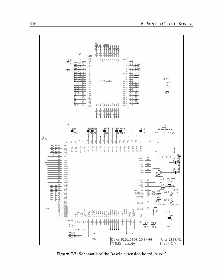
316 E PRINTED CIRCUIT BOARDS
Figure E.7: Schematic of the Baseio extension board, page 2
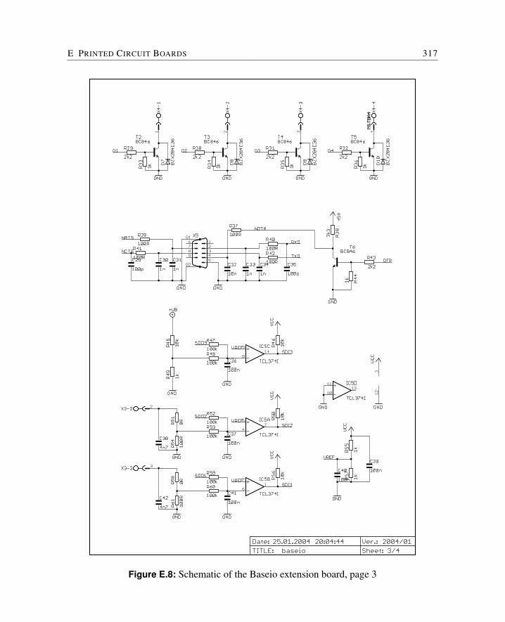
E PRINTED CIRCUIT BOARDS 317
Figure E.8: Schematic of the Baseio extension board, page 3
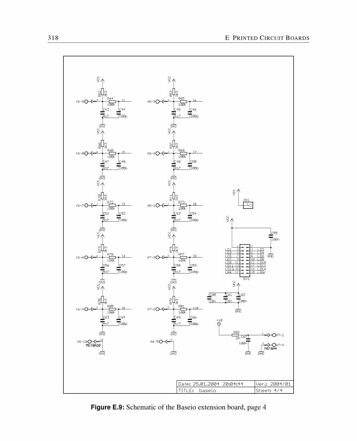
318 E PRINTED CIRCUIT BOARDS
Figure E.9: Schematic of the Baseio extension board, page 4
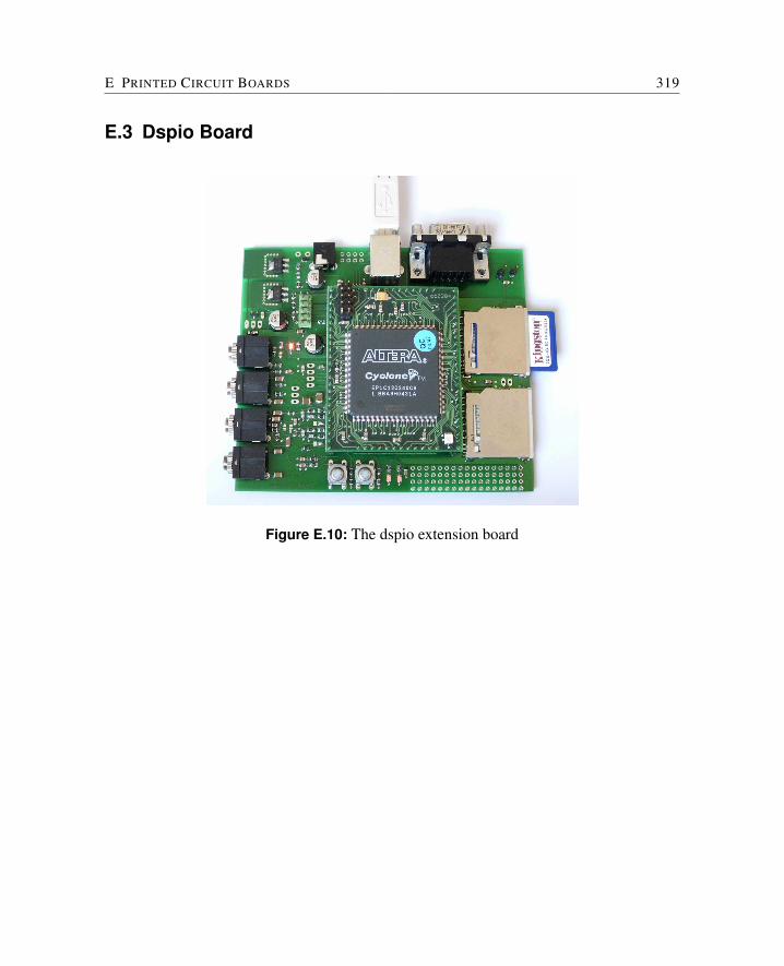
E PRINTED CIRCUIT BOARDS 319
E.3 Dspio Board
Figure E.10: The dspio extension board
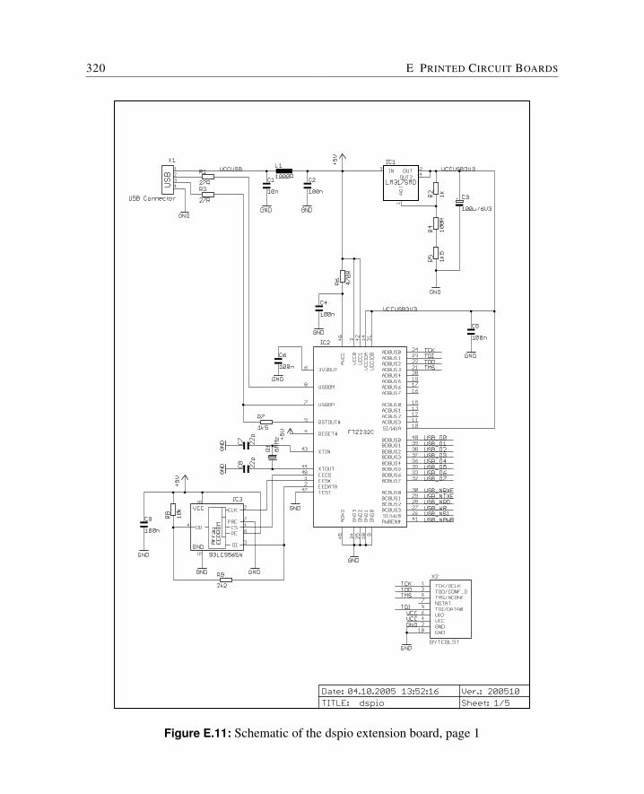
320 E PRINTED CIRCUIT BOARDS
Figure E.11: Schematic of the dspio extension board, page 1
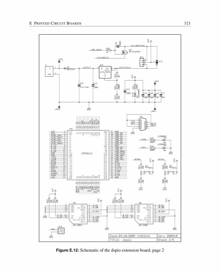
E PRINTED CIRCUIT BOARDS 321
Figure E.12: Schematic of the dspio extension board, page 2
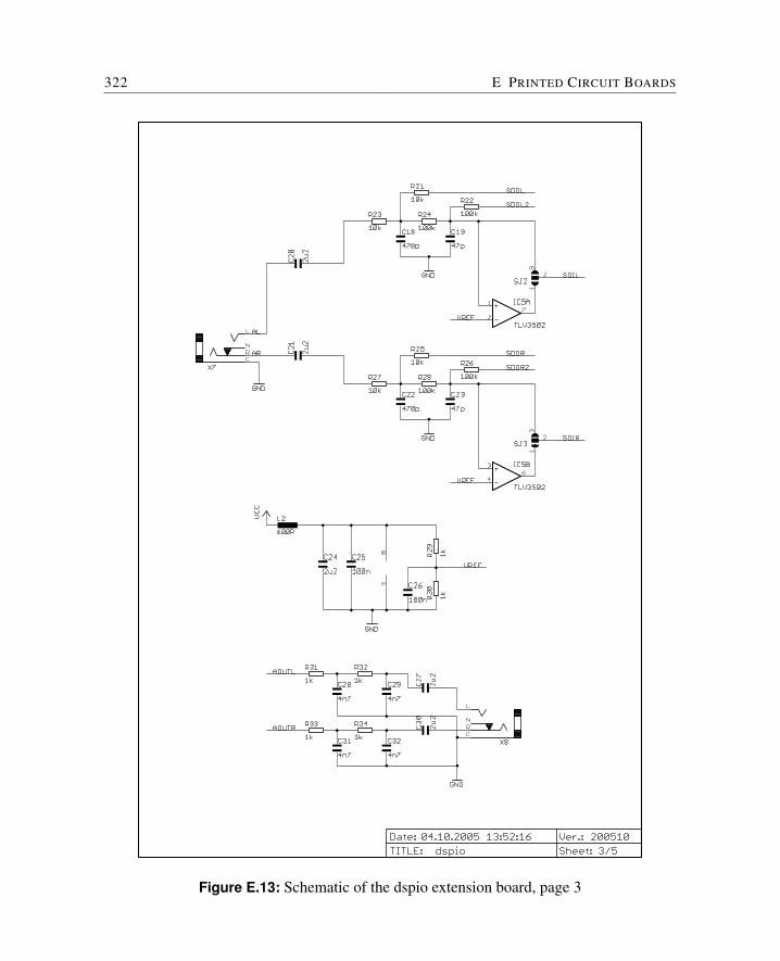
322 E PRINTED CIRCUIT BOARDS
Figure E.13: Schematic of the dspio extension board, page 3
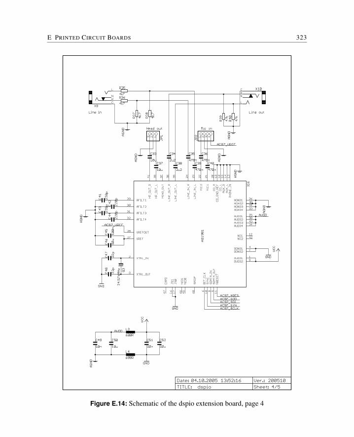
E PRINTED CIRCUIT BOARDS 323
Figure E.14: Schematic of the dspio extension board, page 4
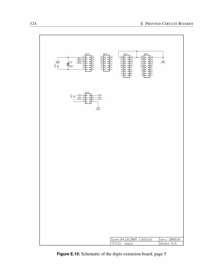
324 E PRINTED CIRCUIT BOARDS
Figure E.15: Schematic of the dspio extension board, page 5
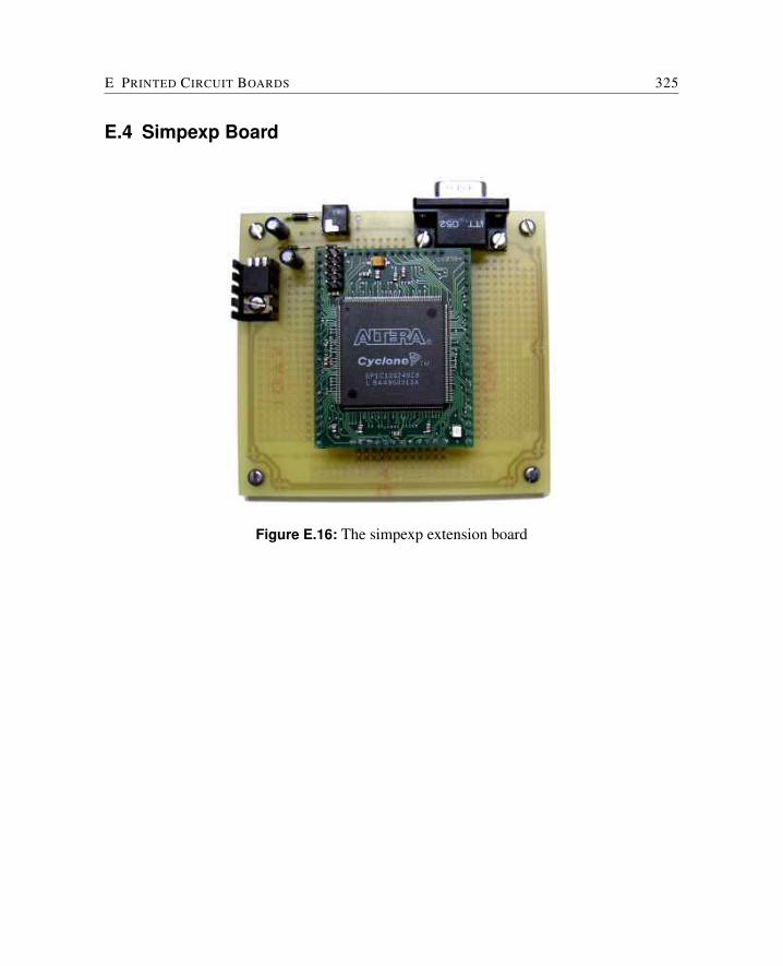
E PRINTED CIRCUIT BOARDS 325
E.4 Simpexp Board
Figure E.16: The simpexp extension board
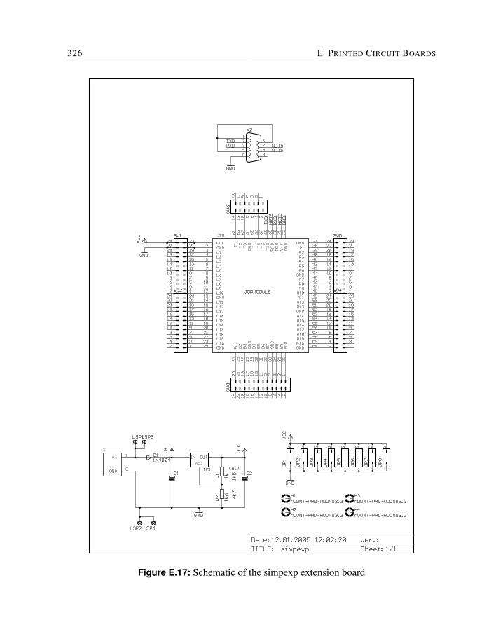
326 E PRINTED CIRCUIT BOARDS
Figure E.17: Schematic of the simpexp extension board
Bibliography
[1] Hija safety critical java proposal. available at http://www.aicas.com/papers/scj.pdf,May 2006.
[2] aJile. aj-100 real-time low power Java processor. preliminary data sheet, 2000.
[3] Altera. Cyclone FPGA Family Data Sheet, ver. 1.2, April 2003.
[4] Altera. Avalon interface specification, April 2005.
[5] Altera. Quartus ii version 7.1 handbook, May 2007.
[6] Aonix. Perc pico 1.1 user manual. http://research.aonix.com/jsc/pico-manual.4-19-08.pdf, April 2008.
[7] ARM. AMBA specification (rev 2.0), May 1999.
[8] ARM. AMBA AXI protocol v1.0 specification, March 2004.
[9] ARM. Jazelle technology: ARM acceleration technology for the Java platform. whitepaper, 2004.
[10] Austin Armbruster, Jason Baker, Antonio Cunei, Chapman Flack, David Holmes,Filip Pizlo, Edward Pla, Marek Prochazka, and Jan Vitek. A real-time Java virtualmachine with applications in avionics. Trans. on Embedded Computing Sys., 7(1):1–49, 2007.
[11] Robert Arnold, Frank Mueller, David Whalley, and Marion Harmon. Boundingworst-case instruction cache performance. In IEEE Real-Time Systems Symposium,pages 172–181, 1994.
[12] Cyrille Artho and Armin Biere. Subroutine inlining and bytecode abstraction to sim-plify static and dynamic analysis. Electronic Notes in Theoretical Computer Science,141(1):109–128, December 2005.
328 BIBLIOGRAPHY
[13] N. C. Audsley, A. Burns, M. F. Richardson, and A. J. Wellings. Hard real-timescheduling: The deadline monotonic approach. In Proceedings 8th IEEE Workshopon Real-Time Operating Systems and Software, Atalanta, 1991.
[14] Joshua Auerbach, David F. Bacon, Bob Blainey, Perry Cheng, Michael Dawson,Mike Fulton, David Grove, Darren Hart, and Mark Stoodley. Design and implemen-tation of a comprehensive real-time java virtual machine. In EMSOFT ’07: Proceed-ings of the 7th ACM & IEEE international conference on Embedded software, pages249–258, New York, NY, USA, 2007. ACM.
[15] Azul. Azul compute appliances. Whitepaper, 2009.
[16] David F. Bacon, Perry Cheng, David Grove, Michael Hind, V. T. Rajan, Eran Ya-hav, Matthias Hauswirth, Christoph M. Kirsch, Daniel Spoonhower, and Martin T.Vechev. High-level real-time programming in java. In EMSOFT ’05: Proceedingsof the 5th ACM international conference on Embedded software, pages 68–78, NewYork, NY, USA, 2005. ACM Press.
[17] David F. Bacon, Perry Cheng, and V. T. Rajan. The metronome: A simpler approachto garbage collection in real-time systems. In Robert Meersman and Zahir Tari,editors, OTM Workshops, volume 2889 of Lecture Notes in Computer Science, pages466–478. Springer, 2003.
[18] David F. Bacon, Perry Cheng, and V. T. Rajan. A real-time garbage collector withlow overhead and consistent utilization. In POPL ’03: Proceedings of the 30th ACMSIGPLAN-SIGACT symposium on Principles of programming languages, pages 285–298, New York, NY, USA, 2003. ACM Press.
[19] Henry G. Baker. List processing in real time on a serial computer. Commun. ACM,21(4):280–294, 1978.
[20] Henry G. Baker. The treadmill: real-time garbage collection without motion sick-ness. SIGPLAN Not., 27(3):66–70, 1992.
[21] Iain Bate, Guillem Bernat, Greg Murphy, and Peter Puschner. Low-level analysisof a portable Java byte code WCET analysis framework. In Proc. 7th InternationalConference on Real-Time Computing Systems and Applications, pages 39–48, Dec.2000.
BIBLIOGRAPHY 329
[22] Iain Bate, Guillem Bernat, and Peter Puschner. Java virtual machine support forportable worst-case execution time analysis. In ISORC. IEEE International Sympo-sium on Object-Oriented Real-Time Distributed Computing, Washington, USA, Jan2002.
[23] Guillem Bernat, Alan Burns, and Andy Wellings. Portable worst-case execution timeanalysis using Java byte code. In Proc. 12th EUROMICRO Conference on Real-timeSystems, Jun 2000.
[24] Thomas Bogholm, Henrik Kragh-Hansen, Petur Olsen, Bent Thomsen, and Kim G.Larsen. Model-based schedulability analysis of safety critical hard real-time Javaprograms. In Proceedings of the 6th international workshop on Java technologiesfor real-time and embedded systems (JTRES 2008), pages 106–114, New York, NY,USA, 2008. ACM.
[25] Greg Bollella, James Gosling, Benjamin Brosgol, Peter Dibble, Steve Furr, and MarkTurnbull. The Real-Time Specification for Java. Java Series. Addison-Wesley, June2000.
[26] Gregory Bollella, Bertrand Delsart, Romain Guider, Christophe Lizzi, and FredericParain. Mackinac: Making HotSpotT M real-time. In ISORC, pages 45–54. IEEEComputer Society, 2005.
[27] Florian Brandner, Tommy Thorn, and Martin Schoeberl. Embedded JIT compila-tion with CACAO on YARI. Technical Report RR 35/2008, Institute of ComputerEngineering, Vienna University of Technology, Austria, June 2008.
[28] Florian Brandner, Tommy Thorn, and Martin Schoeberl. Embedded JIT compi-lation with CACAO on YARI. In Proceedings of the 12th IEEE InternationalSymposium on Object/component/service-oriented Real-time distributed Computing(ISORC 2009), Tokyo, Japan, March 2009. IEEE Computer Society.
[29] Rodney A. Brooks. Trading data space for reduced time and code space in real-time garbage collection on stock hardware. In Prgrm. Chrm. G. L. Steele, Jr., editor,LISP and Functional Programming. Conference Record of the 1984 ACM Sympo-sium, Austin, Texas, August 6-8, 1984, number ISBN 0-89791-142-3, New York,1984. ACM.
330 BIBLIOGRAPHY
[30] Ben Brosgol and Brian Dobbing. Real-time convergence of Ada and Java. In Pro-ceedings of the 2001 annual ACM SIGAda international conference on Ada, pages11–26. ACM Press, 2001.
[31] Jose V. Busquets-Mataix, Juan Jose Serrano, Rafael Ors, Pedro J. Gil, and Andy J.Wellings. Adding instruction cache effect to schedulability analysis of preemptivereal-time systems. In IEEE Real-Time Technology and Applications Symposium(RTAS ’96), pages 204–213, Washington - Brussels - Tokyo, June 1996. IEEE Com-puter Society Press.
[32] C. J. Cheney. A nonrecursive list compacting algorithm. Commun. ACM,13(11):677–678, 1970.
[33] Cyrille Comar, Gary Dismukes, and Franco Gasperoni. Targeting gnat to the javavirtual machine. In Proceedings of the conference on TRI-Ada ’97, pages 149–161.ACM Press, 1997.
[34] Markus Dahm. Byte code engineering with the BCEL API. Technical report, FreieUniversitat Berlin, April 2001.
[35] DCT. Lightfoot 32-bit Java processor core. data sheet, September 2001.
[36] Derivation. Lavacore configurable Java processor core. data sheet, April 2001.
[37] S. Dey, P. Sanchez, D. Panigrahi, L. Chen, C. Taylor, and K. Sekar. Using a soft corein a SOC design: Experiences with picoJava. IEEE Design and Test of Computers,17(3):60–71, July 2000.
[38] Edsger W. Dijkstra, Leslie Lamport, A. J. Martin, C. S. Scholten, and E. F. M. Stef-fens. On-the-fly garbage collection: an exercise in cooperation. Commun. ACM,21(11):966–975, 1978.
[39] Brian Dobbing and Alan Burns. The ravenscar tasking profile for high integrityreal-time programs. In Proceedings of the 1998 annual ACM SIGAda internationalconference on Ada, pages 1–6. ACM Press, 1998.
[40] M. Eden and M. Kagan. The Pentium processor with MMX technology. In Proceed-ings of Compcon ’97, pages 260–262. IEEE Computer Society, 1997.
[41] EJC. The ejc (embedded java controller) platform. Available athttp://www.embedded-web.com/index.html.
BIBLIOGRAPHY 331
[42] Jakob Engblom. Processor Pipelines and Static Worst-Case Execution Time Analy-sis. PhD thesis, Uppsala University, 2002.
[43] Jakob Engblom, Andreas Ermedahl, Mikael Sjodin, Jan Gustafsson, and Hans Hans-son. Worst-case execution-time analysis for embedded real-time systems. Inter-national Journal on Software Tools for Technology Transfer (STTT), 4(4):437–455,August 2003.
[44] Jiri Gaisler. A portable and fault-tolerant microprocessor based on the SPARC v8architecture. In DSN ’02: Proceedings of the 2002 International Conference onDependable Systems and Networks, page 409, Washington, DC, USA, 2002. IEEEComputer Society.
[45] Jiri Gaisler, Edvin Catovic, Marko Isomaki, Kristoffer Carlsson, and Sandi Habinc.GRLIB IP core user’s manual, version 1.0.14. Available at http://www.gaisler.com/,February 2007.
[46] Erich Gamma, Richard Helm, Ralph Johnson, and John M. Vlissides. Design Pat-terns: Elements of Reusable Object-Oriented Software. Addison Wesley Profes-sional, 1994.
[47] James Gosling, Bill Joy, Guy Steele, and Gilad Bracha. The Java Language Specifi-cation Second Edition. The Java Series. Addison-Wesley, Boston, Mass., 2000.
[48] Flavius Gruian, Per Andersson, Krzysztof Kuchcinski, and Martin Schoeberl. Auto-matic generation of application-specific systems based on a micro-programmed javacore. In Proceedings of the 20th ACM Symposium on Applied Computing, EmbeddedSystems track, Santa Fee, New Mexico, March 2005.
[49] Flavius Gruian and Zoran Salcic. Designing a concurrent hardware garbage collectorfor small embedded systems. In Proceedings of Advances in Computer SystemsArchitecture: 10th Asia-Pacific Conference, ACSAC 2005, pages 281–294. Springer-Verlag GmbH, October 2005.
[50] Flavius Gruian and Mark Westmijze. Bluejep: a flexible and high-performance javaembedded processor. In JTRES ’07: Proceedings of the 5th international work-shop on Java technologies for real-time and embedded systems, pages 222–229, NewYork, NY, USA, 2007. ACM.
[51] Jan Gustafsson. Analyzing Execution-Time of Object-Oriented Programs Using Ab-stract Interpretation. PhD thesis, Uppsala University, 2000.
332 BIBLIOGRAPHY
[52] Jan Gustafsson. Worst case execution time analysis of object-oriented programs. InProceedings of the Seventh International Workshop on Object-Oriented Real-TimeDependable Systems (WORDS 2002), pages 71–76, 2002.
[53] Tom R. Halfhill. Imsys hedges bets on Java. Microprocessor Report, August 2000.
[54] David Hardin, Mike Frerking, Philip Wiley, and Gregory Bollella. Getting downand dirty: Device-level programming using the real-time specification for Java. InSymposium on Object-Oriented Real-Time Distributed Computing (ISORC 2002),pages 457–464, 2002.
[55] David S. Hardin. Real-time objects on the bare metal: An efficient hardware re-alization of the Java virtual machine. In Proceedings of the Fourth InternationalSymposium on Object-Oriented Real-Time Distributed Computing, page 53. IEEEComputer Society, 2001.
[56] Trevor Harmon. Interactive Worst-case Execution Time Analysis of Hard Real-timeSystems. PhD thesis, University of California, Irvine, 2009.
[57] Trevor Harmon and Raymond Klefstad. Interactive back-annotation of worst-caseexecution time analysis for Java microprocessors. In Proceedings of the ThirteenthIEEE International Conference on Embedded and Real-Time Computing Systemsand Applications (RTCSA 2007), August 2007.
[58] Trevor Harmon, Martin Schoeberl, Raimund Kirner, and Raymond Klefstad. A mod-ular worst-case execution time analysis tool for Java processors. In Proceedings ofthe 14th IEEE Real-Time and Embedded Technology and Applications Symposium(RTAS 2008), St. Louis, MO, United States, April 2008.
[59] Christopher A. Healy, Robert D. Arnold, Frank Mueller, David B. Whalley, andMarion G. Harmon. Bounding pipeline and instruction cache performance. IEEETrans. Computers, 48(1):53–70, 1999.
[60] Christopher A. Healy, David B. Whalley, and Marion G. Harmon. Integrating thetiming analysis of pipelining and instruction caching. In IEEE Real-Time SystemsSymposium, pages 288–297, 1995.
[61] Reinhold Heckmann, Marc Langenbach, Stephan Thesing, and Reinhard Wilhelm.The influence of processor architecture on the design and results of WCET tools.Proceedings of the IEEE, 91(7):1038–1054, Jul. 2003.
BIBLIOGRAPHY 333
[62] John Hennessy and David Patterson. Computer Architecture: A Quantitative Ap-proach, 3rd ed. Morgan Kaufmann Publishers Inc., Palo Alto, CA 94303, 2002.
[63] John Hennessy and David Patterson. Computer Architecture: A Quantitative Ap-proach, 4th ed. Morgan Kaufmann Publishers, 2006.
[64] Thomas Henties, James J. Hunt, Doug Locke, Kelvin Nilsen, Martin Schoeberl, andJan Vitek. Java for safety-critical applications. In 2nd International Workshop on theCertification of Safety-Critical Software Controlled Systems (SafeCert 2009), Mar.2009.
[65] Teresa Higuera, Valerie Issarny, Michel Banatre, Gilbert Cabillic, Jean-PhilippeLesot, and Frederic Parain. Memory management for real-time Java: an efficientsolution using hardware support. Real-Time Systems Journal, 2002.
[66] Benedikt Huber. Worst-case execution time analysis for real-time Java. Master’sthesis, Vienna University of Technology, Austria, 2009.
[67] Benedikt Huber and Martin Schoeberl. Comparison of implicit path enumerationand model checking based WCET analysis. In Proceedings of the 9th InternationalWorkshop on Worst-Case Execution Time (WCET) Analysis, Dublin, Ireland, July2009. OCG.
[68] IBM. On-chip peripheral bus architecture specifications v2.1, April 2001.
[69] Imsys. ISAJ reference 2.0, January 2001.
[70] Imsys. Im1101c (the Cjip) technical reference manual / v0.25, 2004.
[71] S.A. Ito, L. Carro, and R.P. Jacobi. Making Java work for microcontroller applica-tions. IEEE Design & Test of Computers, 18(5):100–110, 2001.
[72] Richard E. Jones and Rafael Lins. Garbage Collection: Algorithms for AutomaticDynamic Memory Management. Wiley, Chichester, July 1996. With a chapter onDistributed Garbage Collection by R. Lins.
[73] Hermann Kopetz and Gunther Bauer. The time-triggered architecture. Proceedingsof the IEEE, 91(1):112–126, 2003.
[74] Stephan Korsholm, Martin Schoeberl, and Anders P. Ravn. Interrupt han-dlers in Java. In Proceedings of the 11th IEEE International Symposium on
334 BIBLIOGRAPHY
Object/component/service-oriented Real-time distributed Computing (ISORC 2008),Orlando, Florida, USA, May 2008. IEEE Computer Society.
[75] Andreas Krall and Reinhard Grafl. CACAO – A 64 bit JavaVM just-in-time compiler.In Geoffrey C. Fox and Wei Li, editors, PPoPP’97 Workshop on Java for Science andEngineering Computation, Las Vegas, June 1997. ACM.
[76] Jochen Kreuzinger, Uwe Brinkschulte, Matthias Pfeffer, Sascha Uhrig, and TheoUngerer. Real-time event-handling and scheduling on a multithreaded Java micro-controller. Microprocessors and Microsystems, 27(1):19–31, 2003.
[77] Jagun Kwon, Andy Wellings, and Steve King. Ravenscar-Java: A high integrityprofile for real-time Java. In Proceedings of the 2002 joint ACM-ISCOPE conferenceon Java Grande, pages 131–140. ACM Press, 2002.
[78] Chang-Gun Lee, Joosun Hahn, Yang-Min Seo, Sang Lyul Min, Rhan Ha, SeongsooHong, Chang Yun Park, Minsuk Lee, and Chong Sang Kim. Analysis of cache-related preemption delay in fixed-priority preemptive scheduling. IEEE Trans. Com-put., 47(6):700–713, 1998.
[79] Yau-Tsun Steven Li and Sharad Malik. Performance analysis of embedded softwareusing implicit path enumeration. In LCTES ’95: Proceedings of the ACM SIGPLAN1995 workshop on languages, compilers, & tools for real-time systems, pages 88–98,New York, NY, USA, 1995. ACM Press.
[80] Yau-Tsun Steven Li, Sharad Malik, and Andrew Wolfe. Efficient microarchitecturemodeling and path analysis for real-time software. In RTSS ’95: Proceedings of the16th IEEE Real-Time Systems Symposium (RTSS ’95), page 298, Washington, DC,USA, 1995. IEEE Computer Society.
[81] Yau-Tsun Steven Li, Sharad Malik, and Andrew Wolfe. Performance estimation ofembedded software with instruction cache modeling. In Proceedings of the 1995IEEE/ACM international conference on Computer-aided design, pages 380–387.IEEE Computer Society, 1995.
[82] Tim Lindholm and Frank Yellin. The Java Virtual Machine Specification. Addison-Wesley, Reading, MA, USA, second edition, 1999.
[83] C. L. Liu and James W. Layland. Scheduling algorithms for multiprogramming in ahard-real-time environment. J. ACM, 20(1):46–61, 1973.
BIBLIOGRAPHY 335
[84] Thomas Lundqvist and Per Stenstrom. Timing anomalies in dynamically scheduledmicroprocessors. In Proceedings of the 20th IEEE Real-Time Systems Symposium(RTSS 1999), pages 12–21, Washington, DC, USA, 1999. IEEE Computer Society.
[85] Malardalen Real-Time Research Center. WCET benchmarks. Available at http://www.mrtc.mdh.se/projects/wcet/benchmarks.html, accessed 2009.
[86] Stefan Metzlaff, Sascha Uhrig, Jorg Mische, and Theo Ungerer. Predictable dynamicinstruction scratchpad for simultaneous multithreaded processors. In Proceedings ofthe 9th workshop on Memory performance (MEDEA 2008), pages 38–45, New York,NY, USA, 2008. ACM.
[87] Albert F. Niessner and Edward G. Benowitz. RTSJ memory areas and their affectson the performance of a flight-like attitude control system. In Workshop on JavaTechnologies for Real-Time and Embedded Systems (JTRES), LNCS, 2003.
[88] K. Nilsen, L. Carnahan, and M. Ruark. Requirements for real-time extensions forthe Java platform. Available at http://www.nist.gov/rt-java/, September 1999.
[89] S. C. North and J. H. Reppy. Concurrent garbage collection on stock hardware. InG. Kahn, editor, Functional Programming Languages and Computer Architecture,pages 113–133. Springer-Verlag, 1987. Lecture Notes in Computer Science 274;Proceedings of Conference held at Portland, OR.
[90] J. Michael O’Connor and Marc Tremblay. picoJava-I: The Java virtual machine inhardware. IEEE Micro, 17(2):45–53, 1997.
[91] OCP-IP Association. Open core protocol specification 2.1. http://www.ocpip.org/,2005.
[92] Rasmus Pedersen and Martin Schoeberl. Exact roots for a real-time garbage col-lector. In Proceedings of the 4th International Workshop on Java Technologies forReal-time and Embedded Systems (JTRES 2006), pages 77–84, New York, NY, USA,2006. ACM Press.
[93] Rasmus Ulslev Pedersen. Hard real-time analysis of two java-based kernels forstream mining. In Proceedings of the 1st Workshop on Knowledge Discovery fromData Streams (IWKDDS, ECML PKDD 2006), Berlin, Germany, September 2006.
336 BIBLIOGRAPHY
[94] Wade D. Peterson. WISHBONE system-on-chip (SoC) interconnection architecturefor portable IP cores, revision: B.3. Available at http://www.opencores.org, Septem-ber 2002.
[95] Matthias Pfeffer, Theo Ungerer, Stephan Fuhrmann, Jochen Kreuzinger, and UweBrinkschulte. Real-time garbage collection for a multithreaded java microcontroller.Real-Time Systems, 26(1):89–106, 2004.
[96] Christof Pitter. Time-predictable memory arbitration for a Java chip-multiprocessor.In Proceedings of the 6th International Workshop on Java Technologies for Real-timeand Embedded Systems (JTRES 2008), 2008.
[97] Christof Pitter. Time-Predictable Java Chip-Multiprocessor. PhD thesis, ViennaUniversity of Technology, Austria, 2009.
[98] Christof Pitter and Martin Schoeberl. Time predictable CPU and DMA shared mem-ory access. In International Conference on Field-Programmable Logic and its Ap-plications (FPL 2007), pages 317 – 322, Amsterdam, Netherlands, August 2007.
[99] Christof Pitter and Martin Schoeberl. Towards a Java multiprocessor. In Proceedingsof the 5th International Workshop on Java Technologies for Real-time and Embed-ded Systems (JTRES 2007), pages 144–151, Vienna, Austria, September 2007. ACMPress.
[100] Christof Pitter and Martin Schoeberl. Performance evaluation of a Java chip-multiprocessor. In Proceedings of the 3rd IEEE Symposium on Industrial EmbeddedSystems (SIES 2008), Jun. 2008.
[101] Filip Pizlo, J. M. Fox, David Holmes, and Jan Vitek. Real-time java scoped memory:Design patterns and semantics. In Proceedings of the 7th IEEE International Sym-posium on, Object-Oriented Real-Time Distributed Computing (ISORC 2004), pages101–110, 2004.
[102] Thomas B. Preusser, Martin Zabel, and Rainer G. Spallek. Bump-pointer methodcaching for embedded java processors. In Proceedings of the 5th international work-shop on Java technologies for real-time and embedded systems (JTRES 2007), pages206–210, New York, NY, USA, 2007. ACM.
[103] Wolfgang Puffitsch. picoJava-II in an FPGA. Master’s thesis, Vienna University ofTechnology, 2007.
BIBLIOGRAPHY 337
[104] Wolfgang Puffitsch. Supporting WCET analysis with data-flow analysis of Java byte-code. Research Report 16/2009, Institute of Computer Engineering, Vienna Univer-sity of Technology, Austria, February 2009.
[105] Wolfgang Puffitsch and Martin Schoeberl. picoJava-II in an FPGA. In Proceedingsof the 5th International Workshop on Java Technologies for Real-time and Embed-ded Systems (JTRES 2007), pages 213–221, Vienna, Austria, September 2007. ACMPress.
[106] Peter Puschner and Guillem Bernat. Wcet analysis of reusable portable code. InECRTS ’01: Proceedings of the 13th Euromicro Conference on Real-Time Systems,page 45, Washington, DC, USA, 2001. IEEE Computer Society.
[107] Peter Puschner and Alan Burns. A review of worst-case execution-time analysis(editorial). Real-Time Systems, 18(2/3):115–128, 2000.
[108] Peter Puschner and Alan Burns. Writing temporally predictable code. In Proceed-ings of the The Seventh IEEE International Workshop on Object-Oriented Real-TimeDependable Systems (WORDS 2002), pages 85–94, Washington, DC, USA, 2002.IEEE Computer Society.
[109] Peter Puschner and Christian Koza. Calculating the maximum execution time ofreal-time programs. Real-Time Syst., 1(2):159–176, 1989.
[110] Peter Puschner and Anton Schedl. Computing maximum task execution times – agraph-based approach. Journal of Real-Time Systems, 13(1):67–91, Jul. 1997.
[111] Peter Puschner and Andy Wellings. A profile for high integrity real-time Java pro-grams. In 4th IEEE International Symposium on Object-oriented Real-time dis-tributed Computing (ISORC), 2001.
[112] Jan Reineke, Daniel Grund, Christoph Berg, and Reinhard Wilhelm. Timing pre-dictability of cache replacement policies. Journal of Real-Time Systems, 37(2):99–122, Nov. 2007.
[113] Sven Gestegard Robertz and Roger Henriksson. Time-triggered garbage collection:robust and adaptive real-time GC scheduling for embedded systems. In LCTES ’03:Proceedings of the 2003 ACM SIGPLAN conference on Language, compiler, and toolfor embedded systems, pages 93–102, New York, NY, USA, 2003. ACM Press.
338 BIBLIOGRAPHY
[114] Sven Gestegøard Robertz. Automatic memory management for flexible real-timesystems. PhD thesis, Department of Computer Science Lund University, 2006.
[115] RTCA/DO-178B. Software considerations in airborne systems and equipment certi-fication. December 1992.
[116] William J. Schmidt and Kelvin D. Nilsen. Performance of a hardware-assisted real-time garbage collector. In ASPLOS-VI: Proceedings of the sixth international con-ference on Architectural support for programming languages and operating systems,pages 76–85, New York, NY, USA, 1994. ACM Press.
[117] Martin Schoeberl. Using a Java optimized processor in a real world application.In Proceedings of the First Workshop on Intelligent Solutions in Embedded Systems(WISES 2003), pages 165–176, Austria, Vienna, June 2003.
[118] Martin Schoeberl. Real-time scheduling on a Java processor. In Proceedings of the10th International Conference on Real-Time and Embedded Computing Systems andApplications (RTCSA 2004), Gothenburg, Sweden, August 2004.
[119] Martin Schoeberl. Restrictions of Java for embedded real-time systems. In Pro-ceedings of the 7th IEEE International Symposium on Object-Oriented Real-TimeDistributed Computing (ISORC 2004), pages 93–100, Vienna, Austria, May 2004.IEEE.
[120] Martin Schoeberl. A time predictable instruction cache for a Java processor. InOn the Move to Meaningful Internet Systems 2004: Workshop on Java Technologiesfor Real-Time and Embedded Systems (JTRES 2004), volume 3292 of LNCS, pages371–382, Agia Napa, Cyprus, October 2004. Springer.
[121] Martin Schoeberl. Design and implementation of an efficient stack machine. InProceedings of the 12th IEEE Reconfigurable Architecture Workshop (RAW2005),Denver, Colorado, USA, April 2005. IEEE.
[122] Martin Schoeberl. Evaluation of a Java processor. In Tagungsband Austrochip 2005,pages 127–134, Vienna, Austria, October 2005.
[123] Martin Schoeberl. JOP: A Java Optimized Processor for Embedded Real-Time Sys-tems. PhD thesis, Vienna University of Technology, 2005.
BIBLIOGRAPHY 339
[124] Martin Schoeberl. Real-time garbage collection for Java. In Proceedings of the 9thIEEE International Symposium on Object and Component-Oriented Real-Time Dis-tributed Computing (ISORC 2006), pages 424–432, Gyeongju, Korea, April 2006.IEEE.
[125] Martin Schoeberl. Architecture for object oriented programming languages. In Pro-ceedings of the 5th International Workshop on Java Technologies for Real-time andEmbedded Systems (JTRES 2007), pages 57–62, Vienna, Austria, September 2007.ACM Press.
[126] Martin Schoeberl. Mission modes for safety critical Java. In Software Technologiesfor Embedded and Ubiquitous Systems, 5th IFIP WG 10.2 International Workshop(SEUS 2007), volume 4761 of Lecture Notes in Computer Science, pages 105–113.Springer, May 2007.
[127] Martin Schoeberl. SimpCon - a simple and efficient SoC interconnect. In Pro-ceedings of the 15th Austrian Workhop on Microelectronics, Austrochip 2007, Graz,Austria, October 2007.
[128] Martin Schoeberl. A time-triggered network-on-chip. In International Conferenceon Field-Programmable Logic and its Applications (FPL 2007), pages 377 – 382,Amsterdam, Netherlands, August 2007.
[129] Martin Schoeberl. Application experiences with a real-time Java processor. In Pro-ceedings of the 17th IFAC World Congress, Seoul, Korea, July 2008.
[130] Martin Schoeberl. A Java processor architecture for embedded real-time systems.Journal of Systems Architecture, 54/1–2:265–286, 2008.
[131] Martin Schoeberl. JOP: A Java Optimized Processor for Embedded Real-Time Sys-tems. Number ISBN 978-3-8364-8086-4. VDM Verlag Dr. Muller, July 2008.
[132] Martin Schoeberl. Time-predictable computer architecture. EURASIP Journal onEmbedded Systems, vol. 2009, Article ID 758480:17 pages, 2009.
[133] Martin Schoeberl, Stephan Korsholm, Christian Thalinger, and Anders P. Ravn.Hardware objects for Java. In Proceedings of the 11th IEEE International Symposiumon Object/component/service-oriented Real-time distributed Computing (ISORC2008), Orlando, Florida, USA, May 2008. IEEE Computer Society.
340 BIBLIOGRAPHY
[134] Martin Schoeberl and Rasmus Pedersen. WCET analysis for a Java processor. InProceedings of the 4th International Workshop on Java Technologies for Real-timeand Embedded Systems (JTRES 2006), pages 202–211, New York, NY, USA, 2006.ACM Press.
[135] Martin Schoeberl and Wolfgang Puffitsch. Non-blocking object copy for real-timegarbage collection. In Proceedings of the 6th International Workshop on Java Tech-nologies for Real-time and Embedded Systems (JTRES 2008). ACM Press, Septem-ber 2008.
[136] Martin Schoeberl and Peter Puschner. Is chip-multiprocessing the end of real-timescheduling? In Proceedings of the 9th International Workshop on Worst-Case Exe-cution Time (WCET) Analysis, Dublin, Ireland, July 2009. OCG.
[137] Martin Schoeberl, Hans Sondergaard, Bent Thomsen, and Anders P. Ravn. A pro-file for safety critical Java. In 10th IEEE International Symposium on Object andComponent-Oriented Real-Time Distributed Computing (ISORC’07), pages 94–101,Santorini Island, Greece, May 2007. IEEE Computer Society.
[138] Martin Schoeberl and Jan Vitek. Garbage collection for safety critical Java. InProceedings of the 5th International Workshop on Java Technologies for Real-timeand Embedded Systems (JTRES 2007), pages 85–93, Vienna, Austria, September2007. ACM Press.
[139] Alan C. Shaw. Reasoning about time in higher-level language software. IEEE Trans.Softw. Eng., 15(7):875–889, 1989.
[140] Fridtjof Siebert. Hard Realtime Garbage Collection in Modern Object OrientedProgramming Languages. Number ISBN: 3-8311-3893-1. aicas Books, 2002.
[141] International J Consortium Specification. Real-time core extensions, draft 1.0.14.Available at http://www.j-consortium.org/, September 2000.
[142] Guy L. Steele. Multiprocessing compactifying garbage collection. Commun. ACM,18(9):495–508, 1975.
[143] Sun. A brief history of the green project. Available at:http://today.java.net/jag/old/green/.
[144] Sun. Java technology: The early years. Available at:http://java.sun.com/features/1998/05/birthday.html.
BIBLIOGRAPHY 341
[145] Sun. picoJava-II Microarchitecture Guide. Sun Microsystems, March 1999.
[146] Sun. picoJava-II Programmer’s Reference Manual. Sun Microsystems, March 1999.
[147] Systronix. Jstamp real-time native Java module. data sheet.
[148] Y.Y. Tan, C.H. Yau, K.M. Lo, W.S. Yu, P.L. Mok, and A.S. Fong. Design and imple-mentation of a java processor. Computers and Digital Techniques, IEE Proceedings-,153:20–30, 2006.
[149] Sascha Uhrig and Jorg Wiese. jamuth: an IP processor core for embedded Javareal-time systems. In Proceedings of the 5th International Workshop on Java Tech-nologies for Real-time and Embedded Systems (JTRES 2007), pages 230–237, NewYork, NY, USA, 2007. ACM Press.
[150] Andy Wellings and Martin Schoeberl. Thread-local scope caching for real-time Java. In Proceedings of the 12th IEEE International Symposium onObject/component/service-oriented Real-time distributed Computing (ISORC 2009),Tokyo, Japan, March 2009. IEEE Computer Society.
[151] Jack Whitham, Neil Audsley, and Martin Schoeberl. Using hardware methods toimprove time-predictable performance in real-time java systems. In Proceedings ofthe 7th International Workshop on Java Technologies for Real-time and EmbeddedSystems (JTRES 2009), Madrid, Spain, September 2009. ACM Press.
[152] Reinhard Wilhelm, Jakob Engblom, Andreas Ermedahl, Niklas Holsti, StephanThesing, David Whalley, Guillem Bernat, Christian Ferdinand, Reinhold Heckmann,Tulika Mitra, Frank Mueller, Isabelle Puaut, Peter Puschner, Jan Staschulat, and PerStenstrom. The worst-case execution time problem – overview of methods and sur-vey of tools. Trans. on Embedded Computing Sys., 7(3):1–53, 2008.
[153] Paul R. Wilson. Uniprocessor garbage collection techniques. Technical report, Uni-versity of Texas, January 1994. Expanded version of the IWMM92 paper.
[154] Xilinx. Spartan-3 FPGA family: Complete data sheet, ver. 1.2, January 2005.
[155] Tan Yiyu, Richard Li Lo Wan Yiu, Yau Chi Hang, and Anthony S. Fong. A javaprocessor with hardware-support object-oriented instructions. Microprocessors andMicrosystems, 30(8):469–479, 2006.
342 BIBLIOGRAPHY
[156] Taichi Yuasa. Real-time garbage collection on general-purpose machines. Journalof Systems and Software, 11(3):181–198, 1990.
[157] Martin Zabel, Thomas B. Preusser, Peter Reichel, and Rainer G. Spallek. Secure,real-time and multi-threaded general-purpose embedded Java microarchitecture. InPrceedings of the 10th Euromicro Conference on Digital System Design Architec-tures, Methods and Tools (DSD 2007), pages 59–62, Aug. 2007.
[158] R. Zulauf. Entwurf eines Java-Mikrocontrollers und prototypische Implementierungauf einem FPGA. Master’s thesis, University of Karlsruhe, 2000.
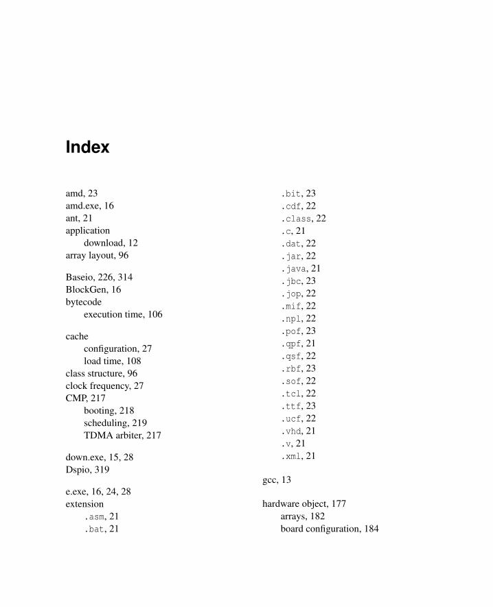
Index
amd, 23amd.exe, 16ant, 21application
download, 12array layout, 96
Baseio, 226, 314BlockGen, 16bytecode
execution time, 106
cacheconfiguration, 27load time, 108
class structure, 96clock frequency, 27CMP, 217
booting, 218scheduling, 219TDMA arbiter, 217
down.exe, 15, 28Dspio, 319
e.exe, 16, 24, 28extension
.asm, 21
.bat, 21
.bit, 23
.cdf, 22
.class, 22
.c, 21
.dat, 22
.jar, 22
.java, 21
.jbc, 23
.jop, 22
.mif, 22
.npl, 22
.pof, 23
.qpf, 21
.qsf, 22
.rbf, 23
.sof, 22
.tcl, 22
.ttf, 23
.ucf, 22
.vhd, 21
.v, 21
.xml, 21
gcc, 13
hardware object, 177arrays, 182board configuration, 184
344 INDEX
creation, 184definition, 179example, 177implementation, 185usage, 182
I/O access, 177interrupt, 61
dispatch, 194handler, 190implementation, 193non-blocking queue, 191synchronization, 190
jar, 22Java coprocessor
Jazelle, 243Java processor
aJile, 229, 246Azul, 249Cjip, 229, 247FemtoJava, 248jamuth, 229, 248jHISC, 249Komodo, 248picoJava, 227, 229, 244SHAP, 229, 249
javac, 2, 22jbi32, 12, 23jbi32.exe, 28JOP porting, 23jop2dat, 13, 20jop blink test, 24jop testmon, 24Jopa, 10, 16, 20, 21, 27jopflash, 13
JOPizer, vii, 10, 12, 16, 22, 25, 30, 39,98, 99
jopser, 13JopSim, 10, 16, 19, 22jopsim, 13jopusb, 13JVM, 94
boot-up, 100class initialization, 98data structures, 94
make, 2, 21, 24memory test, 24method cache, 73
analysis, 119microcode
add, 270and, 268bnz, 287bz, 286dup, 296jbr, 288ld<n>, 291ld opd 16s, 296ld opd 16u, 295ld opd 8s, 295ld opd 8u, 294ldbcstart, 291ldi, 289ldjpc, 294ldmi, 292ldmrd, 290ldmul, 290ldm, 289ldsp, 293ldvp, 293ld, 292
INDEX 345
nop, 287or, 269pop, 268shl, 284shr, 284st<n>, 280stald, 274star, 282stast, 275stbcrd, 279stcp, 278stgf, 276stjpc, 282stmi, 281stmra, 272stmul, 271stmwa, 271stmwd, 273stm, 285stpf, 277stsp, 283stvp, 281st, 280sub, 270ushr, 283wait, 288xor, 269
native method, 25non-blocking queue, 191
object layout, 95
pcsim, 16
quartus pgm, 12, 22
run -all, 21
schematics, 309sim.bat, 21SimpCon, 197
CMP, 205I/O port example, 206interconnection, 204pipelining, 204read transaction, 198ready count, 202signals, 199SRAM interface, 208write transaction, 199
simulationJopSim, 16, 19VHDL, 13, 20
stacksize, 27
system device, 195
UART test, 24udp.Flash, 23USBRunner, 23USBRunner.exe, 16
WCET, 103analysis, 103, 109annotations, 110bytecode timing, 106cache analysis, 117ILP example, 115integer linear programming, 111memory access, 106microcode, 104tool, 120
Xilinx, 11, 18