Joint Example-based Depth Map Super-Resolution

Yanjie Li1, Tianfan Xue2,3, Lifeng Sun1, Jianzhuang Liu2,3,4

1 Information Science and Technology Department, Tsinghua University, Beijing, China2 Department of Information Engineering, The Chinese University of Hong Kong

3 Shenzhen Key Lab for CVPR, Shenzhen Institutes of Advanced Technology, China4 Media Lab, Huawei Technologies Co. Ltd., China

carol.lyj@gmail.com, xtf009@ie.cuhk.edu.hk, sunlf@tsinghua.edu.cn, jzliu@ie.cuhk.edu.hk

Abstract—The fast development of time-of-flight (ToF) cam-eras in recent years enables capture of high frame-rate 3Ddepth maps of moving objects. However, the resolution of depthmap captured by ToF is rather limited, and thus it cannot bedirectly used to build a high quality 3D model. In order tohandle this problem, we propose a novel joint example-baseddepth map super-resolution method, which converts a lowresolution depth map to a high resolution depth map, using aregistered high resolution color image as a reference. Differentfrom previous depth map SR methods without training stage,we learn a mapping function from a set of training samplesand enhance the resolution of the depth map via sparsecoding algorithm. We further use a reconstruction constraint tomake object edges sharper. Experimental results show that ourmethod outperforms state-of-the-art methods for depth mapsuper-resolution.

Keywords-Depth map; Super-resolution (SR); Registeredcolor image; Sparse representation;

I. INTRODUCTION

A depth map, representing the relative distance of each

object point to the video camera, is widely used in 3D object

presentation. Current depth sensors for capturing depth maps

can be grouped into two categories: passive sensors and

active sensors. Passive sensors, like a stereo vision camera

system, is time-consuming and not accurate at textureless or

occluded regions. On the contrary, active sensors generate

more accurate result, and two most popular active sensors

are laser scanners and Time-of-Flight (ToF) sensors. Laser

scanners, despite the high-quality depth map they generated,

they have limited applications in static environments, as they

can only measure a single point at a time. Compared with the

these sensors, ToF sensors are much cheaper and can capture

a depth map of fast moving objects, which are drawing more

and more interest in recent years [1], [2]. However, a depth

map captured by a ToF sensor has very low resolution. For

example, the resolution of PMD CamCube 3.0 is 200× 200resolution and the resolution of MESA SR 4000 is 176×144.

In order to improve the quality, a postprocess step is needed

to enhance the resolution of the depth map [3], [4], which

is called depth map super-resolution (SR) in the literature.

Some previous SR approaches [3] recover a high resolu-

tion depth map from multiple depth maps of the same static

(a) (b) (c)

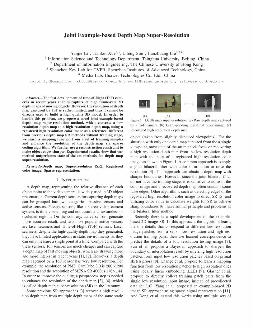
Figure 1. Depth map super-resolution. (a) Raw depth map captured

by a ToF camera. (b) Corresponding registered color image. (c)

Recovered high resolution depth map.

object (taken from slightly displaced viewpoints). For the

situation with only one depth map captured from the a single

viewpoint, most state-of-the-art methods focus on recovering

a high resolution depth map from the low resolution depth

map with the help of a registered high resolution color

image, as shown in Figure 1. A common approach is to apply

a joint bilateral filter with color information to raise the

resolution [4]. This approach can obtain a depth map with

sharper boundaries. However, since the joint bilateral filter

do not have the training stage, it is sensitive to noise in the

color image and a recovered depth map often contains some

false edges. Other algorithms, such as detecting edges of the

registered high resolution color image to direct SR [5] and

utilizing color value to calculate weights for SR to achieve

sharp boundaries [6], have similar principle and problems as

the bilateral filter method.

Recently there is a rapid development of the example-

based 2D image SR. In this approach, the algorithm learns

the fine details that correspond to different low resolution

image patches from a set of low resolution and high res-

olution training pairs, then use learned correspondence to

predict the details of a low resolution testing image [7].

Sun et al. propose a Bayesian approach to sharpen the

boundary of interpolation result by inferring high resolution

patches from input low resolution patches based on primal

sketch priors [8]. Change et al. propose to learn a mapping

function from low resolution patches to high resolution ones

using locally linear embedding (LLE) [9]. Glasner et al.

propose to directly collect training patch pairs from the

single low resolution input image, instead of precollected

data set [10]. Yang et al. proposed an example-based 2D

image SR approach using sparse signal representation [11].

And Dong et al. extend this works using multiple sets of

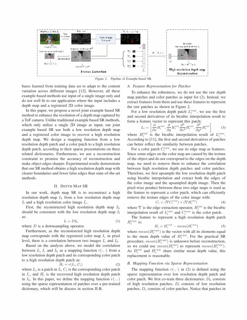
R e g i s t e r e d 2 D m a p I cL o w � r e s o l u t i o n d e p t h m a p I lE d g eE x t r a c t i o n E d g e m a p R e f i n e d e d g e m a pI n t e r p o l a t i o n L iI n t e r p o l a t e d d e p t h m a p H i n t T e x t u r e e d g eR e m o v a l

P a t c h H i i n t i n H i n tF e a t u r e E x t r a c t i o n H i S R r e s u l t :H i g h � r e s o l u t i o n d e p t h m a p I hH i g h r e s o l u t i o n d e p t h m a pR e c o n s t r u c t i o nC iP a t c h L i i n I lP a t c h C i i n I c H i = r ( L i , C i )r a wr a w P a t c h H i r a w i n I h

Figure 2. Pipeline of Example-based SR.

bases learned from training data set to adapt to the content

variation across different images [12]. However, all these

example-based methods use input of a single image only and

do not well fit to our application where the input includes a

depth map and a registered 2D color image.

In this paper, we propose a novel joint example based SR

method to enhance the resolution of a depth map captured by

a ToF camera. Unlike traditional example based SR methods,

which only utilize a single 2D image as input, our joint

example based SR use both a low resolution depth map

and a registered color image to recover a high resolution

depth map. We design a mapping function from a low

resolution depth patch and a color patch to a high resolution

depth patch, according to their sparse presentations on three

related dictionaries. Furthermore, we use a reconstruction

constraint to promise the accuracy of reconstruction and

make object edges sharper. Experimental results demonstrate

that our SR method obtains a high resolution depth map with

clearer boundaries and fewer false edges than state-of-the-art

methods.

II. DEPTH MAP SR

In our work, depth map SR is to reconstruct a high

resolution depth map Ih from a low resolution depth map

Il and a high resolution color image Ic.

First, the reconstructed high resolution depth map Ih

should be consistent with the low resolution depth map Il

as:Il = DIh (1)

where D is a downsampling operator.

Furthermore, as the reconstructed high resolution depth

map corresponds with the registered color map Ic in pixel

level, there is a correlation between two images Ic and Ih.

Based on the analysis above, we model the correlation

between Il, Ic and Ih as a mapping function r(·, ·) from a

low resolution depth patch and its corresponding color patch

to a high resolution depth patch as:Hi = r(Li, Ci) (2)

where Li is a patch in Il, Ci is the corresponding color patch

in Ic, and Hi is the recovered high resolution depth patch

in Ih. In this paper, we define the mapping function r(·, ·)using the sparse representation of patches over a pre-trained

dictionary, which will be discuss in section II-B.

A. Feature Representation for Patches

To enhance the robustness, we do not use the raw depth

map patches and color patches as input for (2). Instead, we

extract features from them and use these features to represent

the raw patches as shown in Figure 2.

For a low resolution depth patch Lrawi , we use the first

and second derivatives of its bicubic interpolation result to

form a feature vector to represent this patch:

Li =

[

∂

∂xH

int

i ,∂

∂yH

int

i

∂2

∂x2H

int

i ,∂2

∂y2H

int

i

]

(3)

where Hinti is the bicubic interpolation result of Lraw

i .

According to [11], the first and second derivatives of patches

can better reflect the similarity between patches.

For a color patch Crawi , we use its edge map as features.

Since some edges on the color map are caused by the texture

of the object and do not correspond to the edges on the depth

map, we need to remove them to enhance the correlation

between high resolution depth patches and color patches.

Therefore, we first upsample the low resolution depth patch

using bicubic interpolation and extract both the edges of

the color image and the upsampled depth image. Then the

pixel-wise product between these two edge maps is used as

the feature to represent a color patch, which can efficiently

remove the texture edges of the color image with:

Ci = (∇Craw

i ) × (∇Hint

i ) (4)

where ∇ is the edge extraction operator, Hinti is the bicubic

interpolation result of Lrawi and Craw

i is the color patch.

The feature to represent a high resolution depth patch

Hrawi is:

Hi = Hraw

i − mean(Hraw

i ) (5)

where mean(Hrawi ) is the vector with all its elements equal

to the mean depth value of Hrawi . For the practical SR

procedure, mean(Hrawi ) is unknown before reconstruction,

so we could use mean(Hinti ) to represent mean(Hraw

i ).As Hint

i and Hrawi share similar mean depth value, this

replacement is reasonable.

B. Mapping Function via Sparse Representation

The mapping function r(·, ·) in (2) is defined using the

sparse representation over low resolution depth patch and

color patch. We first co-train three dictionaries: Dh consists

of high resolution patches; Dl consists of low resolution

patches; Dc consists of color patches. Notice that patches in

Dl, Dc and Dh are correspondent, i.e., the ith low resolution

patch in Dl corresponds with the ith high resolution patch

in Dh and the ith color patch in Dc. The details of training

will be introduced in section II-C.

Then for each new input low resolution patch Li and

its corresponding color patch Ci, we can find the output

high resolution patch Hi as follows. We first find a sparse

representation of these two patches on the dictionaries Dl

and Dc respectively. Here we enforce Li and Ci have

the same sparse coefficients on dictionaries Dl and Dc.

Then the high resolution patch is recovered using the same

coefficients. The mapping function is defined as:Hi = r(Li, Ci) = Dhα

∗i

where: α∗i = argmin

||αi||0≤ǫ

{λl||Dlαi − Li||22 + λc||Dcαi − Ci||

22 + f(Hi, Li)}

(6)

where αi is the coefficient vector consisting of all the

coefficients, each of Dh, Dl and Dc is a matrix with

each prototype patch being a column vector, λl and λc are

two balance parameters, and || · ||0 denotes the l0-norm. f

is a constraint function to ensure reconstruction constraint

defined in (1). The detailed definition of f(Hi, Li) is given

in section II-D.

Here we enforce the sparsity constraint ||α||0 ≤ ǫ for two

reasons: first, with the sparsity constraint, it is reasonable

to reconstruct Hi using coefficients αi, which are the linear

coefficients for representing Li (or Ci) using patches in Dl

(or Dc). Second, as discussed in [13], if a high resolution

patch Hi can be represented as a sufficient sparse linear

combination of patches in Dh, it can be perfectly recovered

from a low resolution patch.

Same as previous works on sparse representation, we re-

place l0-norm by l1-norm in (6) for computational efficiency.

As discussed in [13], the l1-norm constraint still ensures the

sparsity of the coefficients αi. Then while ignoring f , (6)

becomes

α∗i = argmin

||αi||1≤ǫ

{λl||Dlαi − Li||22 + λc||Dcαi − Ci||

22} (7)

C. Dictionary Training

The dictionaries Dl, Dc and Dh are trained from a set of

corresponded low resolution depth patches, high resolution

depth patches (ground-truth) and color patches. The training

is to minimize the following estimation error:

E =∑

i

||r(Li, Ci) − Hi||22 (8)

Combining (7) and (8), we have:

minDl,Dc,Dh,αi

∑

i

λl||Dlαi−Li||22+λc||Dcαi−Ci||

22 + ||Dhαi−Hi||

22

subject to: ||αi||1 ≤ ǫ∀i (9)

In our work, we use about 105 patches for training and

after training, each dictionary contains only 1024 patches.

We use dictionary size which is much smaller than the

number of training samples for robustness and efficiency.

The above dictionary training formulation (9) is common in

sparse representation, and can be solved using an iterative

optimization method [14], [11].

D. Mapping Function with a Reconstruction Constraint

The reconstruction constraint defined in (1) is important

for SR. Without this constraint, the downsampling result of

the recovered high resolution depth map is not guaranteed

to be close to the input low resolution depth map, and a

serious artifact will appear when the mapping function fails

to get the correct high resolution patch.

Directly combining the reconstruction constraint (1) with

the mapping function defined in previous section is not easy.

So we first apply an upsampling operator U on both sides

of (1), resulting in:

UIl = UDIh ≈ Ih (10)

The simplest way for upsampling is the bicubic interpola-

tion. However, there is an obvious blurring effect on the

boundaries of the object in the depth map Hint obtained

from the interpolation. To remove this effect, we apply

the joint-bilateral filter proposed in [4], which can generate

clearer object boundaries than Hint:

Hb(x) =

1

Z

∑

x′∈N(x)

e−

||x−x′||22θ2

s−

||C(x)−C(x′)||22θ2

c Hint(x′) (11)

where Z is the normalization factor, N(x) is a neighborhood

of x, C(x) is the RGB color vector of the pixel at position

x in the registered color image Ic, and Hint(x) is the depth

value of the pixel at position x in Hint. After filtering,

pixels with similar colors tend to have similar depth values.

Therefore, the filtering result Hb normally has a sharper

boundary compared with the interpolation result Hint.

Then we use Hb = UIl ≈ Ih as the reconstruction

constraint. Let Hbi be a patch on Hb. Then the recovered

high resolution depth patch Hi in Ih should be as near to Hbi

as possible. We use the l2-norm to model this reconstruction

constraint f and add it to the mapping function (7):

Hi = Dhα∗i

where: α∗i = argmin

||α||1≤ǫ

{λl||Dlα − Li||22 + λc||Dcα − Ci||

22 (12)

+ λr||Dhα − Hb

i ||22}

where λr is the weight for reconstruction constraint. (12) is

a LASSO linear regression problem, and can be efficiently

solved by [15]. In the experiment, we simply set all the

weighting parameters λl, λc and λr to 1.

E. Proposed Joint Example-based Depth Map SR

Utilizing the final mapping function as (12), the proposed

example-based depth map SR algorithm can be summarized

in Algorithm 1. To remove the blocking effect, we divide

the low resolution depth map into overlapping patches,

and obtain the high resolution patch using the mapping

function (12). Then we combine these patches to a whole

high resolution depth map by averaging the depth values

over the overlapping regions.

Algorithm 1 Proposed Example-based depth map SR

Input: A low-resolution depth map Il, the corresponding colorimage Ic and dictionaries Dl, Dc and Dh

1) Upsample Il to the same resolution as Ic, and apply bilateralfilter (11) to it to get filtered image Hb

2) for each patch of Li in Il

3) Get the corresponding color patch Ci and depthpatch Hb

i from Ic and Hb respectively

4) Get the high resolution depth patch Hi from Li, Ci

and Hb

i by solving the optimization problem (12)

5) endfor

6) Recover the whole high resolution depth map by combiningall patches Hi obtained in step 4

III. EXPERIMENTS AND RESULTS

A. Comparison with other approaches

We collect 34 pairs of color images and depth maps from

4 videos of Philips 3DTV. The low resolution depth maps

for training are obtained from high resolution depth maps

by a Gaussian blurring and downsampling. In the training

stage, we only train dictionaries to increase the resolution

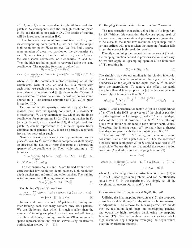
of a depth map by factor 2. Examples of training patches

are shown in Figure 3. For larger magnifying factors, such

as 8, we get the high resolution depth map by applying the

SR three times. For each training patch triple (low and high

resolution depth patches and color patches), we randomly

select a 4 × 4 patche from the low resolution depth maps

and its corresponding 8×8 patches from the high resolution

depth maps and color images. We extract 100,000 patch

triples from the 34 groups of images to train the dictionaries

Dl, Dh and Dc, each of which contains 1024 patches after

training.

To evaluate the performance of our algorithm, we compare

it with five other SR methods. Among them, there are three

methods use no registered color image information: bicubic

interpolation (Bc), bilateral filtering using only depth infor-

mation (D-Bi)) and sparse representation method proposed

by Yang et al. in [11] (Sc-Y). The other two methods are the

state-of-the-art methods designed specially for depth map

SR, which take into account the registered color image

information: the joint-bilateral filtering as defined in [4]

(J-Bi) and the algorithm using registered color image to

direct calculation of weights for interpolation as in [6] (C-

W). From another angle, among the five methods, Sc-Y

is an example-based algorithm, just like our method. The

same training set, and the dictionary size, patch size, and

overlapping size are used in both our algorithm and Sc-Y.

The other four methods do not have a training stage. The

testing set consists of 13 images randomly selected from 6

videos. Four of these videos are also from Philips 3DTV

website as the training set (Girl, Football, Dandelion and

Frisbee) and two are from Microsoft Research Asia website

(Ballet and Breakdancers).

We first evaluate the performance of these six algorithms

Figure 3. Example of training patches. The first row shows color patches,the second row shows corresponding low resolution depth patches, and thirdrow shows corresponding high resolution depth patches.

Table IROOT MEAN SQUARE ERROR (RMSE) FOR SIX TESTING VIDEOS

Average RMSETestVideos

Ours Sc-Y J-Bi C-W D-Bi Bc

Girl 6.5 7.03 7.3 9.24 7.35 7.36

Football 4.94 5.27 6.25 7.12 6.37 6.39

Dandelion 5.09 5.49 6.18 5.91 6.23 6.23

Frisbee 8.24 8.84 9.37 10.89 9.46 9.47

Ballet 8.83 9.63 9.98 9.42 10.16 10.25

Breakdancer 5.44 5.68 5.72 6.79 5.74 5.76

with a magnifying factor 8. A quantitative result is given

in Table I. It shows that our algorithm achieves the best

results on all the testing sequences. RMSE also shows that

the example-based algorithms (our algorithm and Sc-Y)

outperform those non-training methods. And the methods

taking into account the registered color image information

(J-Bi and C-W) perform better than the ones using only low

resolution depth map (D-Bi and Bc).

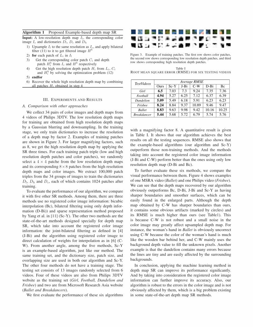
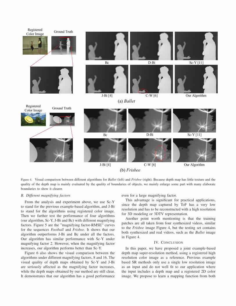
To further evaluate these six methods, we compare the

visual performance between them. Figure 4 shows examples

of one MSRA video (Ballet) and one Philips video (Frisbee).

We can see that the depth maps recovered by our algorithm

obviously outperforms Bc, D-Bi, J-Bi and Sc-Y as having

sharper boundaries and smoother surfaces, which can be

easily found in the enlarged parts. Although the depth

map obtained by C-W has sharper boundaries than ours,

it contains some obvious artifacts (marked by circles) and

its RMSE is much higher than ours (see Table1). This

is because C-W is not robust and a small noise in the

color image may greatly affect upsampled depth map. For

instance, the woman’s hand in Ballet is obviously uncorrect

using C-W because the color of the woman’s hand is much

like the wooden bar behind her, and C-W mainly uses the

background depth value to fill the unknown pixels. Another

example is that the dandelion contains many errors because

the lines are tiny and are easily affected by the surrounding

backgrounds.

In conclusion, applying the machine learning method in

depth map SR can improve its performance significantly.

And by taking into consideration the registered color image

information can further improve its accuracy. Also, our

algorithm is robust to the errors in the color image and is not

obviously affected by them, which is a big problem existing

in some state-of-the-art depth map SR methods.

(b) Frisbee

Registered

Color ImageGround Truth

Bc D-Bi Sc-Y [11]

Our AlgorithmC-W [6]J-Bi [4]

(a) Ballet

Registered

Color ImageGround Truth

Bc D-Bi Sc-Y [11]

Our AlgorithmC-W [6]J-Bi [4]

Figure 4. Visual comparison between different algorithms for Ballet (left) and Frisbee (right). Because depth map has little texture and the

quality of the depth map is mainly evaluated by the quality of boundaries of objects, we mainly enlarge some part with many elaborate

boundaries to show it clearer.

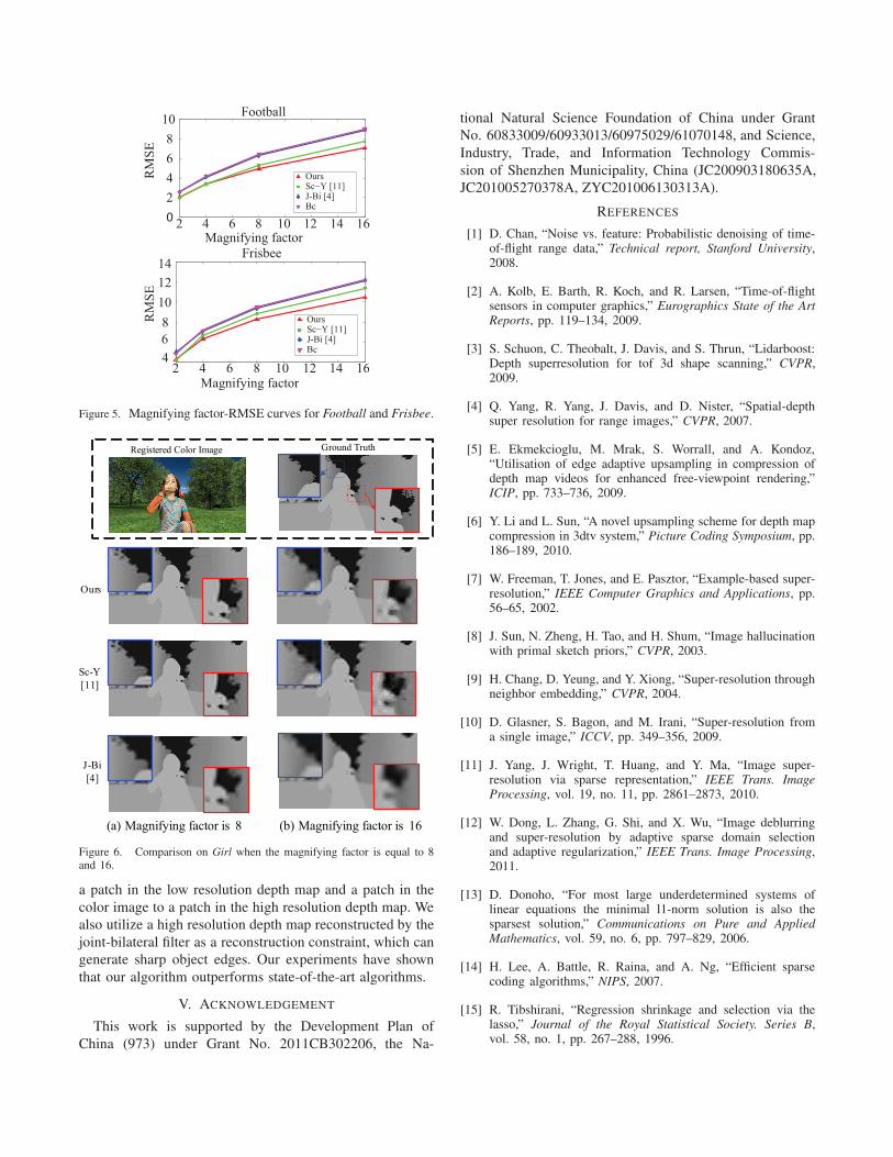
B. Different magnifying factors

From the analysis and experiment above, we use Sc-Y

to stand for the previous example-based algorithm, and J-Bi

to stand for the algorithms using registered color image.

Then we further test the performance of four algorithms

(our algorithm, Sc-Y, J-Bi and Bc) with different magnifying

factors. Figure 5 are the ”magnifying factor-RMSE” curves

for the sequences Football and Frisbee. It shows that our

algorithm outperforms J-Bi and Bc under all the factors.

Our algorithm has similar performance with Sc-Y under

magnifying factor 2. However, when the magnifying factor

increases, our algorithm performs better than Sc-Y.

Figure 6 also shows the visual comparison between the

algorithms under different magnifying factors, 8 and 16. The

visual quality of depth maps obtained by Sc-Y and J-Bi

are seriously affected as the magnifying factor increases,

while the depth maps obtained by our method are still clear.

It demonstrates that our algorithm has a good performance

even for a large magnifying factor.

This advantage is significant for practical applications,

since the depth map captured by ToF has a very low

resolution and has to be reconstructed with a high resolution

for 3D modeling or 3DTV representation.

Another point worth mentioning is that the training

patches are all taken from four synthesized videos, similar

to the Frisbee image Figure 4, but the testing set contains

both synthesized and real videos, such as the Ballet image

in Figure 4.

IV. CONCLUSION

In this paper, we have proposed a joint example-based

depth map super-resolution method, using a registered high

resolution color image as a reference. Previous example

based SR methods only use a single low resolution image

as an input and do not well fit to our application where

the input includes a depth map and a registered 2D color

image. We propose to learn a mapping function from both

2 4 6 8 10 12 14 160

2

4

6

8

10Football

Magnifying factor

RM

SE

OursSc−Y [11]J-Bi [4]Bc

2 4 6 8 10 12 14 164

6

8

10

12

14Frisbee

Magnifying factor

RM

SE

OursSc−Y [11]J-Bi [4]Bc

Figure 5. Magnifying factor-RMSE curves for Football and Frisbee.

(b) Magnifying factor is 16(a) Magnifying factor is 8

Ours

Sc-Y

[11]

J-Bi

[4]

Registered Color Image Ground Truth

Figure 6. Comparison on Girl when the magnifying factor is equal to 8and 16.

a patch in the low resolution depth map and a patch in the

color image to a patch in the high resolution depth map. We

also utilize a high resolution depth map reconstructed by the

joint-bilateral filter as a reconstruction constraint, which can

generate sharp object edges. Our experiments have shown

that our algorithm outperforms state-of-the-art algorithms.

V. ACKNOWLEDGEMENT

This work is supported by the Development Plan of

China (973) under Grant No. 2011CB302206, the Na-

tional Natural Science Foundation of China under Grant

No. 60833009/60933013/60975029/61070148, and Science,

Industry, Trade, and Information Technology Commis-

sion of Shenzhen Municipality, China (JC200903180635A,

JC201005270378A, ZYC201006130313A).

REFERENCES

[1] D. Chan, “Noise vs. feature: Probabilistic denoising of time-of-flight range data,” Technical report, Stanford University,2008.

[2] A. Kolb, E. Barth, R. Koch, and R. Larsen, “Time-of-flightsensors in computer graphics,” Eurographics State of the ArtReports, pp. 119–134, 2009.

[3] S. Schuon, C. Theobalt, J. Davis, and S. Thrun, “Lidarboost:Depth superresolution for tof 3d shape scanning,” CVPR,2009.

[4] Q. Yang, R. Yang, J. Davis, and D. Nister, “Spatial-depthsuper resolution for range images,” CVPR, 2007.

[5] E. Ekmekcioglu, M. Mrak, S. Worrall, and A. Kondoz,“Utilisation of edge adaptive upsampling in compression ofdepth map videos for enhanced free-viewpoint rendering,”ICIP, pp. 733–736, 2009.

[6] Y. Li and L. Sun, “A novel upsampling scheme for depth mapcompression in 3dtv system,” Picture Coding Symposium, pp.186–189, 2010.

[7] W. Freeman, T. Jones, and E. Pasztor, “Example-based super-resolution,” IEEE Computer Graphics and Applications, pp.56–65, 2002.

[8] J. Sun, N. Zheng, H. Tao, and H. Shum, “Image hallucinationwith primal sketch priors,” CVPR, 2003.

[9] H. Chang, D. Yeung, and Y. Xiong, “Super-resolution throughneighbor embedding,” CVPR, 2004.

[10] D. Glasner, S. Bagon, and M. Irani, “Super-resolution froma single image,” ICCV, pp. 349–356, 2009.

[11] J. Yang, J. Wright, T. Huang, and Y. Ma, “Image super-resolution via sparse representation,” IEEE Trans. ImageProcessing, vol. 19, no. 11, pp. 2861–2873, 2010.

[12] W. Dong, L. Zhang, G. Shi, and X. Wu, “Image deblurringand super-resolution by adaptive sparse domain selectionand adaptive regularization,” IEEE Trans. Image Processing,2011.

[13] D. Donoho, “For most large underdetermined systems oflinear equations the minimal l1-norm solution is also thesparsest solution,” Communications on Pure and AppliedMathematics, vol. 59, no. 6, pp. 797–829, 2006.

[14] H. Lee, A. Battle, R. Raina, and A. Ng, “Efficient sparsecoding algorithms,” NIPS, 2007.

[15] R. Tibshirani, “Regression shrinkage and selection via thelasso,” Journal of the Royal Statistical Society. Series B,vol. 58, no. 1, pp. 267–288, 1996.