jean-pierre macquart

Transients & Variableswith SKA2 & AA-MIDJean-Pierre Macquart

Transients, Variables and AA-MID

The case for high sensitivity & large FoV

Exciting new results FRBs

• Thoughts on their significance Gravitational Waves

Other known knowns Bread and butter science

How does AA-MID fit in the picture?

2


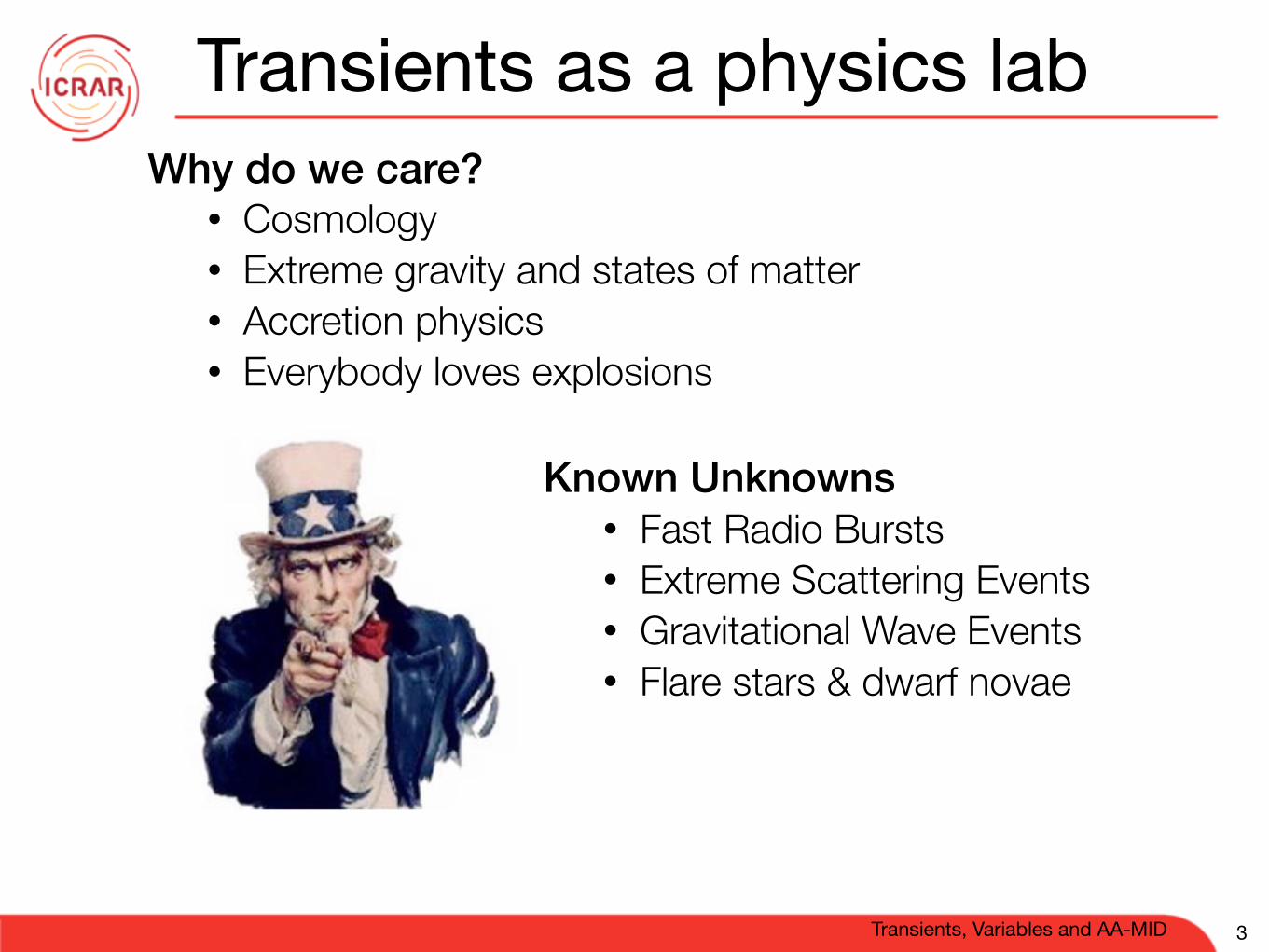
Transients as a physics labWhy do we care?

• Cosmology • Extreme gravity and states of matter • Accretion physics • Everybody loves explosions

3

Known Unknowns • Fast Radio Bursts • Extreme Scattering Events • Gravitational Wave Events • Flare stars & dwarf novae


Known Knowns & Known UnknownsTime-domain - bursty and generally coherent

• Pulsars including Magnetar bursts, Transitional XRBs, Giant Pulses, RRATs

• Fast Radio Bursts • Bursty emission from exoplanet-star systems, brown

dwarfs • Cosmic rays, lunar neutrinos (so far only SKA1_LOW)

Image domain - incoherent synchrotron or thermal • X-ray binaries • Tidal Disruption Events • Novae & Flare stars • Intra-day variable quasars/Extreme Scattering Events • System mergers/gravitational wave events

4


Fast transients as cosmological probes

5

energy distribution across the band in FRB 110220is characterized by bright bands ~100 MHz wide(Fig. 2); the SNRs are too low in the other threeFRBs to quantify this behavior (2). Similar spec-tral characteristics are commonly observed in theemission of high-|b| pulsars.

With four FRBs, it is possible to calculate anapproximate event rate. The high-latitude HTRUsurvey region is 24% complete, resulting in 4500square degrees observed for 270 s. This cor-responds to an FRB rate ofRFRBðF e 3 Jy msÞ ¼1:0þ0:6

−0:5 % 104sky−1day−1, where the 1-s uncer-tainty assumes Poissonian statistics. The MWforeground would reduce this rate, with increasedsky temperature, scattering, and dispersion forsurveys close to the Galactic plane. In the ab-sence of these conditions, our rate implies that17þ9

−7 , 7þ4−3 , and 12þ6

−5 FRBs should be found inthe completed high- and medium-latitude partsof the HTRU (1) and Parkes multibeam pulsar(PMPS) surveys (18).

One candidate FRB with DM > DMMW hasbeen detected in the PMPS [ jbj < 5 (5, 19)].This burst could be explained by neutron staremission, given a small scale-height error;however, observations have not detected anyrepetition. No excess-DM FRBs were detected ina burst search of the first 23% of the medium-latitude HTRU survey [jbj < 15 (20)].

The event rate originally suggested forFRB 010724, R010724 ¼ 225 sky−1 day−1 (4), isconsistent with our event rate given a Euclid-ean universe and a population with distance-independent intrinsic luminosities (sourcecount, NºF−3=2) yielding RFRB ðF e 3 Jy msÞe 102RFRBðF010724 e 150 Jy msÞ.

There are no known transients detected atgamma-ray, x-ray, or optical wavelengths orgravitational wave triggers that can be temporallyassociated with any FRBs. In particular there is

Fig. 2. A dynamic spectrum showing the frequency-dependent delay of FRB 110220. Time is measured relativeto the time of arrival in the highest frequency channel. For claritywe have integrated 30 time samples, corresponding to the dis-persion smearing in the lowest frequency channel. (Inset) Thetop, middle, and bottom 25-MHz-wide dedispersed subband usedin the pulse-fitting analysis (2); the peaks of the pulses arealigned to time = 0. The data are shown as solid gray lines andthe best-fit profiles by dashed black lines.

Table 1. Parameters for the four FRBs. The position given is the center of the gain pattern of the beamin which the FRB was detected (half-power beam width ~ 14 arc min). The UTC corresponds to the arrivaltime at 1581.804688MHz. The DM uncertainties depend not only on SNR but also on whether a and b areassumed (a ¼ −2; no scattering) or fit for; where fitted, a and b are given. The comoving distance wascalculated by using DMHost = 100 cm−3 pc (in the rest frame of the host) and a standard, flat-universeLCDM cosmology, which describes the expansion of the universe with baryonic and dark matter and darkenergy [H0 = 71 km s−1Mpc−1,WM=0.27,WL =0.73;H0 is the Hubble constant andWM andWL are fractionsof the critical density of matter and dark energy, respectively (29)]. a and b are from a series of fits usingintrinsic pulse widths of 0.87 to 3.5ms; the uncertainties reflect the spread of values obtained (2). The observedwidths are shown; FRBs 110627, 110703, and 120127 are limited by the temporal resolution due to dis-persion smearing. The energy released is calculated for the observing band in the rest frame of the source (2).

FRB 110220 FRB 110627 FRB 110703 FRB 120127

Beam rightascension ( J2000)

22h 34m 21h 03m 23h 30m 23h 15m

Beam declination( J2000)

−12° 24′ −44° 44′ −02° 52′ −18° 25′

Galactic latitude,b (°)

−54.7 −41.7 −59.0 −66.2

Galactic longitude,l (°)

+50.8 +355.8 +81.0 +49.2

UTC (dd/mm/yyyyhh:mm:ss.sss)

20/02/201101:55:48.957

27/06/201121:33:17.474

03/07/201118:59:40.591

27/01/201208:11:21.723

DM (cm−3 pc) 944.38 T 0.05 723.0 T 0.3 1103.6 T 0.7 553.3 T 0.3DME (cm

−3 pc) 910 677 1072 521Redshift, z (DMHost =

100 cm−3 pc)0.81 0.61 0.96 0.45

Co-moving distance,D (Gpc) at z

2.8 2.2 3.2 1.7

Dispersion index, a −2.003 T 0.006 – −2.000 T 0.006 –Scattering index, b −4.0 T 0.4 – – –Observed width

at 1.3 GHz, W (ms)5.6 T 0.1 <1.4 <4.3 <1.1

SNR 49 11 16 11Minimum peak

flux density Sn(Jy)1.3 0.4 0.5 0.5

Fluence at 1.3 GHz,F (Jy ms)

8.0 0.7 1.8 0.6

SnD2 (× 1012 Jy kpc2) 10.2 1.9 5.1 1.4Energy released, E (J) ~1039 ~1037 ~1038 ~1037

www.sciencemag.org SCIENCE VOL 341 5 JULY 2013 55

REPORTS

on

Ju

ly 4

, 2

01

3w

ww

.scie

nce

ma

g.o

rgD

ow

nlo

ad

ed

fro

m

0.0 0.2 0.4 0.6 0.8 1.00

500

1000

1500

zcolumndensity

pccm

3 ?redshift (distance)di

sper

sion

mea

sure

(DM

)

We can – directly detect every single baryon along the line of sight! – use the DM-redshift relation as a cosmic ruler – measure turbulence on sub 108m scales at distances of ~1Gpc – probe IGM physics: primordial magnetic field & energy deposition

Dark energy:

identity unknown,

~73 percent

Dark matter:

identity unknown,

~23 percent

Luminous matter:

stars and luminous gas 0.4 percent

radiation 0.005 percent

Other nonluminous components

intergalactic gas 3.6 percent,

neutrinos 0.1 percent

supermassive black holes

0.004 percent

“Missing” Baryons

Galaxies

X-ray coronae

Ly-α absorption systems

see both Macquart et al., Fender et al. in the SKA Science book


Extraordinary FRB properties• Bright Fluences up to ~10 Jy ms

– 19 events from Parkes (Lorimer et al. 2007;Thornton et al. 2013;Champion et al. 2016)

– 1 at Arecibo (Spitler et al. 2014)

– 1 at Green Bank (forthcoming)

• Distant Extremely high dispersion measures for objects above the Galactic plane (375-1500 pc/cm3) – Not obviously associated with nearby galaxies

• Common Inferred event rate ~ 2-5 x103 sky-1 day-1

• Scattered At least 4 exhibit temporal smearing of order several milliseconds (much larger than expected due to scattering in the Milky Way)

6

110m GBT 64m Parkes 300m Arecibo


Where are the missing baryons?FRB dispersion can directly answer this question

• Missing baryons location an important element of galaxy halo accretion and feedback

• Most dark matter found in galaxy halos, but most baryonic matter outside this scale (>100kpc)

• How do we determine its distribution?

7

𝛾 McQuinn 2014

Fast Radio Bursts

Dark Energy - FRBs as cosmic rulersFRBs measure the dark energy equation of state:

How does w evolve with time?

• The term c dt/dz is a ruler that measures the curvature of the Universe • Measure the DM as a function of redshift

8

w =p

DM =

nedl

ne

c dt

dz

dz

Zhou et al. 2014

H and He ionization fractions

baryonic density curvature due to matter curvature due to dark energy w(z): equation of state

DMIGM(z) = b3H0c

8Gmp

z

0

(1 + z)fIGM

34Xe,H(z) + 1

8Xe,He(z)

M(1 + z)3 + DE(1 + z)3[1+w(z)]

1/2dz

: Universe curvature terms


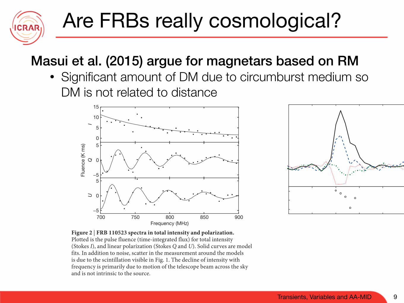
Are FRBs really cosmological?

Masui et al. (2015) argue for magnetars based on RM • Significant amount of DM due to circumburst medium so

DM is not related to distance

9

5 2 4 | N A T U R E | V O L 5 2 8 | 2 4 / 3 1 D E C E M B E R 2 0 1 5

LETTERRESEARCH

By fitting a model to the burst data, we found the detection signifi-cance to be over 40σ, with fluence 3.79(15) K ms at our centre spectral frequency of 800 MHz. The burst has a steep spectral index of −7.8(4), which we attribute to telescope motion. The peak antenna temperature at 800 MHz is 1.16(5) K. We do not know the location of the source within the GBT beam profile, but if the source location were at beam centre where the antenna gain is 2 K Jy−1 the measured antenna tem-perature would translate to 0.6 Jy. Off-centre the antenna has lower gain so, as in previously reported bursts, this is a lower limit to the FRB flux. The intrinsic full-width at half-maximum (FWHM) duration of the burst (with scattering removed) is 1.74(17) ms, similar to the widths of previously reported FRBs.

Allowing the dispersion relation to vary in the model, we found that the dispersive delay is proportional to tdelay ≈ ν−1.998(3), in close agreement to the expected ν−2 dependence for a cold, diffuse plasma. Following Katz22, this provides an upper limit on the density of elec-trons in the dispersing plasma of ne < 1.3 × 107 cm−3 at 95% confi-dence and a lower limit on the size of the dispersive region of d > 10 astronomical units (au). This limit improves upon limits from previ-ous bursts22–24 and rules out a flare star as the source of FRB 110523, because stellar coronas are denser and less extended by at least an order of magnitude25. Flare stars are the last viable Galactic-origin model for FRB sources, so we take the source to be extragalactic.

We found strong linear polarization, with linearly polarized fraction 44(3)%. Linearly polarized radio sources exhibit Faraday rotation of the polarization angle on the sky by angle ϕFar = RM × λ2, where λ is the wavelength and the rotation measure RM (a measure of magnetization) is the line-of-sight component of the magnetic field weighted by the electron density:

∫= .µ

−−

n B lRM 0 812 rad mcm G

dpc

2 e3

We detected the expected λ2 modulation pattern in the polarization as shown in Fig. 2. The best-fitting RM is −186.1(1.4) rad m−2. All radio telescopes have polarization leakage, an instrument-induced false polarization of unpolarized sources. We mapped the leakage at GBT across the beam profile and throughout the passband and found that leakage can produce false linear polarization as large as 10% and false circular polarization as large as 30%. Leakage-produced apparent polarization lacks the λ2 wavelength dependence that we see in the linear polarization data and cannot produce the 44% polarization we

detect so we conclude that the linear polarization is of astronomical origin rather than due to leakage.

The rotation measure and dispersion measure we detected imply an electron-weighted average line-of-sight component of the magnetic field of 0.38 µ G, compared to typical large-scale fields of ∼10 µ G in spiral galaxies26. This field strength is a lower limit for the magnetized region owing to cancellations along the line of sight. Also, the mag-netized region may only weakly overlap the dispersing region and so electron weighting may not be representative.

The magnetization we detected is probably local to the FRB source rather than in the Milky Way or the intergalactic medium. Models of Faraday rotation within the Milky Way predict a contribution of RM = 18(3) rad m−2 for this line of sight, while the intergalactic medium can contribute at most | RM| = 6 rad m−2 on a typical line of sight from this redshift27.

We detected a rotation of the polarization angle over the pulse dura-tion of − 0.25(5) rad ms−1, shown in Fig. 3. Such rotation of polarization is often seen in pulsars and is attributed to the changes in the projection of the magnetic field compared to the line of sight as the neutron star rotates28.

We also detected circular polarization at roughly the 23% level, but that level of polarization might be due to instrumental leakage. Faraday rotation is undetectable for circular polarization, so the λ2 modulation we use to identify astronomical linear polarization is not available as a tool to rule out leakage. For these reasons we do not have confidence that the detected circular polarization is of astronomical origin.

Radio emissions are often scattered: lensing by plasma inhomoge-neities creates multiple propagation paths, with individual delays. We observed two distinct scattering timescales in the FRB 110523 data, indicating the presence of two scattering screens. In five previous FRB detections an exponential tail in the pulse profile was detected, interpreted as the superposition of delayed versions of the narrower intrinsic profile. The average scattering time constant for FRB 110523 is 1.66(14) ms at 800 MHz, with the expected decrease with spectral frequency as shown in Extended Data Fig. 2. We also detected scin-tillation, the variation of intensity with frequency due to multi-path interference. We measured a scintillation de-correlation bandwidth of fdc = 1.2(4) MHz (see Extended Data Fig. 3), indicating a second source

0

5

10

15

I

−5

0

5

Q

700 750 800 850 900Frequency (MHz)

−5

0

5

UFl

uenc

e (K

ms)

Figure 2 | FRB 110523 spectra in total intensity and polarization. Plotted is the pulse fluence (time-integrated flux) for total intensity (Stokes I), and linear polarization (Stokes Q and U). Solid curves are model fits. In addition to noise, scatter in the measurement around the models is due to the scintillation visible in Fig. 1. The decline of intensity with frequency is primarily due to motion of the telescope beam across the sky and is not intrinsic to the source.

−0.2

0.0

0.2

0.4

0.6

0.8

1.0

Ant

enna

tem

pera

ture

(K)

I

P+

P×

V

−10 −5 0 5 10 15 20Time (ms)

0

−20

−40\ (d

eg)

Figure 3 | Polarized pulse profiles averaged over spectral frequency. Plotted is total intensity (I), linear polarization (P+ and P×), and circular polarization (V, which may be instrumental). Before taking the noise-weighted mean over frequency, the data are scaled to 800 MHz using the best-fit spectral index and the linear polarization is rotated to compensate for the best-fit Faraday rotation. The linear polarization basis coordinates are aligned with (+), and rotated with respect to (×), the mean polarization over time. The bottom panel shows the polarization angle (where measurable) in these coordinates. The error bars show the standard deviation of 10,000 simulated measurements with independent noise realizations.

© 2015 Macmillan Publishers Limited. All rights reserved


Are FRBs Cosmological?Keane et al. (2016) present evidence that FRB bursts are clean and that DM maps directly to the DMIGM

• Host galaxy at z=0.492. • Argument hinges upon correct identification of host galaxy

• ATCA followup of Parkes detection shows a fading transient • Williams, Berger et al. dispute this (in a Telegram and arXiv only) • Coincidence only that host distance implies ΩIGM=4.9±1.3%?

10

LETTERRESEARCH

2 | N A T U R E | V O L 0 0 0 | 0 0 M O N T H 2 0 1 6

FWHM ≈ 0.8 arcsec) using the Faint Object Camera and Spectrograph (FOCAS) on Subaru on 2015 November 03. This yielded a spectrum con-sistent with a reddened elliptical galaxy at z = 0.492 ± 0.008 (Fig. 3). An ear-lier 1-h observation, on a night which was not spectrophotometric, using the Deep Imaging Multi-Object Spectrograph (DEIMOS) on the Keck telescope, was also taken and found to be consistent with the Subaru result.

Dispersion in the intergalactic medium is related to the cosmic density of ionized baryons ΩIGM and the redshift19,20 according to the following expression:

∫ΩΩ Ω

=π

( + ′) ( ′) ′( + ′) +

( )Λ.

cHGm

z f z zz

DM 38

1 d[ 1 ]

1z

IGM0 IGM

p 0e

3m

0 5

Here, we take DMIGM = DMFRB − DMMW − DMhalo − DMhost(1 + z)−1 (see Methods). It is appropriate to account for a Milky Way halo con-tribution21 of DMhalo = 30 cm−3 pc and we derive 189 cm−3 pc for DMMW (the DM for the rest of the Milky Way, excluding its halo, that is, the non-dark-matter component of the Milky Way) from the NE2001 Galactic electron density model14. An elliptical galaxy can be modelled22 with a modified version of NE2001 with an average rest-frame

value of ∼37 cm−3 pc. The NE2001 components are uncertain at the 20% level14, and there is an additional uncertainty of ∼100 cm−3 pc owing to line-of-sight inhomogeneities in the intergalactic medium10. We therefore obtain:

Ω =⎛

⎝⎜⎜⎜⎜. ⎞

⎠⎟⎟⎟⎟⎟. ± . ( )

f0 88 0 049 0 013 2IGM

e

The ionization factor is fe = 1 for fully ionized hydrogen, whereas allowing for a helium abundance of 25%, fe = 0.88 is appropriate20.

Figure 1 | The FRB 150418 radio signal. a, A waterfall plot of the FRB signal with 15 frequency sub-bands across the Parkes observing bandwidth, showing the characteristic quadratic time–frequency sweep. To increase the signal-to-noise ratio, the time resolution is reduced by a factor of 14 from the raw 64-µs value. b, The pulse profile of the FRB signal with the total intensity, linear and circular polarization flux densities shown as black, purple and green lines respectively. c, The polarization position angle is shown with 1σ error bars, for each 64-µs time sample where the linear polarization was greater than twice the uncertainty in the linear polarization.

Table 1 | Summary of FRB 150418 observed and derived properties

Event time at 1,382 MHz 2015 April 18 04:29:07.056 UTCEvent time at infinite frequency 2015 April 18 04:29:05.370 UTCParkes beam number 4, inner ringBeam FWHM diameter 14.1′Beam centre (RA, dec.) 07 h 16 min 30.9 s, −19° 02′ 24.4′′Beam centre (l, b) 232.684°, −3.261°Galaxy position (RA, dec.) ATCA epoch 1

07 h 16 min 35(3) s, −19° 00′ 40(1)′′

Galaxy position (l, b) ATCA epoch 1

232.6654(1)°, −3.2348(3)°

Signal-to-noise ratio 39Observed width, Wobs 0.8 ± 0.3 msFRB dispersion measure 776.2(5) cm−3 pcDispersion index, β −2.00(1)Milky Way dispersion measure 188.5 cm−3 pcRedshift, z 0.492(8)Peak flux density, S1382 MHz > . − .

+ .2 2 0 30 6 Jy (beam centre)

> . − .+ .2 4 0 4

0 5 Jy (galaxy position)Fluence, F1382 MHz (Jy ms) . − .

+ .1 9 0 81 1 Jy ms (beam centre)

. − .+ .2 0 0 8

1 2 Jy ms (galaxy position)Linear polarization, L/I 8.5 ± 1.5%Circular polarization, |V|/I <4.5% (3σ)Rotation measure 36 ± 52 rad m−2

Spectral index, α α > −3.0 (3σ, Parkes-MWA)α = +1.3 ± 0.5 (Parkes)

Comoving distance 1.88 gigaparsecsLuminosity distance 2.81 gigaparsecsEnergy ×−

+8 1051 38 ergs (galaxy position)

Luminosity >1.3 × 1042 ergs s−1 (galaxy position)The peak flux density is a band average and a lower limit due to the intrinsic width not being resolved; similarly luminosity is a lower limit. The energy quoted is the product of the band-averaged fluence, the blueshifted effective bandwidth of the observations and the square of the luminosity distance. MWA denotes the Murchison Widefield Array.

1,200

1,250

1,300

1,350

1,400

1,450

1,500

0 0.2 0.4 0.6 0.8 1.0

Freq

uenc

y (M

Hz)

Time since 18 April 2015 04:29:06.7 UTC (s)

a

0

0.5

1.0

1.5

0 1 2 3

Flux

den

sity

(arb

itrar

y un

its)

Time (ms)

b

–60

0

60

Pos

ition

angl

e (°

)

c

Figure 2 | The FRB host galaxy radio light curve . Detections have 1σ error bars, and 3σ upper limits are indicated with arrows. The afterglow event appears to last ∼6 days, after which time the brightness settles at the quiescent level for the galaxy. Here mjd denotes modified Julian day.

0

50

100

150

200

250

300

350

400

0 50 100 150 200 250

Pea

k br

ight

ness

(mic

roja

nsky

per

bea

m)

Days since MJD 57130

ATCA 5.5 GHz

ATCA 7.5 GHz

GMRT 610 MHz

GMRT 1.4 GHz A fading transient or a variable source?


Correct host ID?

No evidence for an AGN (but may be obscured by dust)

11

LETTER RESEARCH

0 0 M O N T H 2 0 1 6 | V O L 0 0 0 | N A T U R E | 3

From fitting ΛCDM cosmological models to Wilkinson Microwave Anisotropy Probe (WMAP) observations one derives12 the cosmic density of all baryons Ωbaryons = 0.046 ± 0.002. Of these, about 10% are not ionized or are in stellar interiors23 so that we expect to meas-ure a cosmic density of ionized baryons in the intergalactic medium of ΩIGM ≈ 0.9 × Ωbaryons ≈ 0.041 ± 0.002. Thus, our measurement independently verifies the ΛCDM model and the WMAP observa-tions, and constitutes a direct measurement of the ionized material associated with all of the baryonic matter in the direction of the FRB, including the so-called “missing baryons”24. Alternatively, if we take ΩIGM ≡ 0.041, our measurements show that DMhost is negligible.

FRB localization allows us to correct a number of observable quantities that are corrupted by the unknown gain correction factor owing to a lack of knowledge of the true position within the telescope beam. Accounting for the frequency-dependent beam response25 we can derive a true spectral index for the FRB. We obtain α = +1.3 ± 0.5 for a fit centred at 1.382 GHz.

Similarly, we derive a corrected flux density and fluence, and these, in com-bination with the redshift measurement, enable us to derive the distances, the energy released, the luminosity and other parameters (Table 1).

In considering the nature of the progenitor we first consider the host galaxy. An upper limit to the star-formation rate can be determined from the upper limit Hα luminosity indicated by the Subaru spectrum (see Methods) to be ≤0.2M yr−1, where M is the solar mass. Such a low star-formation rate implies, in the simplest interpretation, that FRB models directly related to recent star formation such as magnetar flares or blitzars are disfavoured. This problem might be avoided if either some residual star formation occurred in an otherwise ‘dead’ galaxy, or if the FRB originated in one of the many satellite galaxies that are expected to surround an elliptical galaxy at this redshift, but that cannot be resolved in our observations. Failing these, the lack of star formation favours models such as compact merger events. This may be supported by the existence of the ∼6-day radio transient, which we interpret as

Figure 3 | Optical analysis of the FRB host galaxy. a, A wide-field composite false-colour RGB (red–green–blue) image, overplotted with the half-power beam pattern of the Parkes multi-beam receiver. Panels b and c show successive zooms on the beam 4 region, and on the fading ATCA transient location respectively. P200 K s denotes the Palomar telescope 200-inch Ks band. Panel d is further zoomed in with the error ellipses for the ATCA transient, as derived from both the first and

second epoch, overplotted. e, The Subaru FOCAS spectrum de-reddened with E(B − V) = 1.2, smoothed by five pixels and fitted to an elliptical galaxy template at z = 0.492, denoted by the blue line. Common atomic transitions observed in galaxies are denoted by vertical dashed lines and yellow lines denote bright night sky lines. The Subaru r′ and i′ filter bandpasses are denoted by light red and grey background shading. The red line is the 1σ per pixel uncertainty (not smoothed).

7 h 14 min 00.00 s7 h 16 min 00.00 s

7 h 18 min 00.00 s7 h 20 min 00.00 s

Right ascension (J2000)

−19° 20′ 00.0″

−20° 20′ 00.0″

−19° 40′ 00.0″

−19° 00′ 00.0″

−18° 40′ 00.0″

−20° 00′ 00.0″

Dec

linat

ion

(J20

00)

a WISEW1/W2/W3

e

b

c

WISEW1/W2/W3

Subaru r ′/Subaru i ′/P200 K s

d Subaru r ′/Subaru i ′/P200 K s

Observed wavelength (Å)

0.0

0.2

0.4

0.6

0.8

1.0

1.2

1.4

Flux

(×10

−17

erg

s−1 c

m−2

Å−1

)

O II

H8

H7

H6

Ca_

H&

K

Hδ

CH

G-b

and

Hγ

Hβ

O II

I

Mg

I

Na

I

Hα

6,000 7,000 8,000 9,000 10,000


Are FRBs Cosmological?

12

1,250

1,300

1,350

1,400

1,450

1,500

Obs

.fre

quen

cy(M

Hz)

Burst 1

0 3 6

S/N

1,250

1,300

1,350

1,400

1,450

1,500

Obs

.fre

quen

cy(M

Hz)

Burst 2

0 3 6

S/NBurst 3

0 3 6

S/N

1,250

1,300

1,350

1,400

1,450

1,500

Obs

.fre

quen

cy(M

Hz)

Burst 4

0 4 8

S/NBurst 5

0 3

S/N

2012-11-02MJD 56233

2015-05-17MJD 57159

2015-06-02MJD 57175(two scans)

Figure 2 FRB 121102 burst morphologies and spectra. The central greyscale (linearlyscaled) panels show the total intensity versus observing frequency and time, after cor-recting for dispersion to DM=559 pc cm3. The data are shown with 10 MHz and 0.524 msfrequency and time resolution, respectively. The diagonal striping at low radio frequenciesfor Bursts 6, 7 and 9 is due to RFI that is unrelated to FRB 121102. The upper sub-panelsare burst profiles summed over all frequencies. The band-corrected burst spectra areshown in the right sub-panels. The signal-to-noise scales for the spectra are shown oneach sub-panel. All panels are arbitrarily and independently scaled.

12

Spitler et al. (2016) report a repeating FRB

• Spectrum is all over the place

• Argue that it favours magnetar origin - but magnetars are not bright enough to be visible at cosmological distances

• Are there two populations of FRB?


Evidence of FRB Cosmological Origin

Observations show there is a 4.7:1 difference in the detection rate between high (>30 deg) and low latitude (Petroff et al. 2014)

Interstellar scintillation explains this dependence: also implies source counts are non-Euclidean (dN/dSν ~ Sν-3.5) (Macquart & Johnston 2015)

13

latitude Hours on sky Events Rate (h/event)|b|<15 1927.7 2 960

30<|b|<45 2128.85 7 300|b|>45 1030.0 6 170


Scintillation enhancement

14

• In the regime of strong diffractive scintillation, the probability distribution of amplifications at high latitude is

• The differential source counts follow a distribution

• where δ=0 for a Euclidean universe that is homogeneously populated with transients

pa(a) = ea

p(S) / S5/2+

0 1 2 3 4 50.0

0.2

0.4

0.6

0.8

1.0

amplify

deam

plify

High Galactic Latitude

0 1 2 3 4 50

1

2

3

4

5

Low Galactic Latitude

vs

pa

pa

a

a


FRB enhancement

15

• Observed flux density: Z=Sν x a: 4 Macquart & Johnston

0.001 0.01 0.1 1 10

10-5

0.001

0.1

10

1000

105

pZ(Z)/K

Z/Smax

Smin

Smax

Fig. 1.— The distribution of observed flux densities pZ(Z) (blue line) for an initial flux density distribution (purple line) that is nonzeroover the range S

min

< Z < Smax

and with = 0. The e↵ect of the di↵ractive scintillations is to draw out the high end of the distributioninto a tail that decreases like Z1 exp(Z), increase the di↵erential event counts over the range S

min

Z . Smax

and to extend the lowluminosity component of the distribution to zero flux density.

For completeness, we also consider the flux density distribution where a large number of scintles, N , contribute tothe overall measurement of the flux density across the observing bandwidth, using eq.(3):

pZ,N (Z) = KZ 5

2

+

(2

1

4

2p

1

2

N

N

5 2

4

1

F1

2 3

4;1

2;1

22

N

+p2

7 2

4

1

F1

2 1

4;3

2;1

22

N

),(8)

where1

F1

is a confluent hypergeometric function, and we have taken the limits Smin

= 0 and Smax

! 1 in order tomake the problem analytically tractable. The expression in the curly brackets represents the correction to the eventrate over the non-scintillating signal.In the limit N ! 1 this distribution approaches the intrinsic distribution given by eq.(5). For finite values of N ,

there is still some small increase in the event rate over the range Smin

Z . Smax

, but this diminishes rapidly withN , as shown in Figure 2. The important point is that for the small scintillation bandwidths typical of di↵ractivescintillation closer than 30 to the Galactic plane where one has N & 30 for typical HTRU observing parameters, theoverall enhancement is less than 5%.

10 1005020 2003015 15070

1.00

1.05

1.10

1.15

1.20

pZ

,N(Z

)/K

Z5

/2+δ

N

δ=-1/2

δ=0

δ=1/2

Fig. 2.— The amplification of the event rate with the number of scintles that contributes to the flux density in the limit in which N islarge and S

min

! 0 and Smax

! 1.

2.2. Flux density distribution measured with a single-pixel or multibeam receiver

A complication arises in comparing the observed flux density distribution of FRBs with foregoing results becauseall FRB detections have hitherto been detected with non-interferometric radio telescopes. Each event is detected atan unknown angular distance from the beam centre, and the observed signal-to-noise is attenuated by an unknownamount according to the beam shape. However, although the e↵ect of beam attenuation is unknown for any givenevent, it is nonetheless possible to derive its statistical e↵ect on a population of events. We quantify this e↵ect here.Our analysis is informed by two aspects of the HTRU survey:

original distribution

observed distribution

• Enhance the event rate by a factor

52

• Draws out tail of distribution

the transient events. The quantity R is proportional to the integral event counts (i.e.the number detected above the threshold flux density S0), and the differential count isgiven by differentiating with respect to S0.

For simplicity of notation, we therefore write the probability distribution of eventflux densities (akin to differential event number counts) as

pS(S) = KS−5/2+δ0 , (3)

where K can be derived by comparing pS with eq.(2), and the factor δ takes into accountevolution in the progenitor population and the non-Euclidean geometry of the Universeat z ! 1. (Similar effects in the quasar number counts give rise to effects with δ ∼0.5.) Furthermore, if these events occur only at cosmological distances, there will be amaximum flux density Smax that is attainable, and pS(S) = 0 for S > Smax.

0.2 0.5 1.0 2.0 5.0 10.0 20.0

10 4

0.01

1

100

pZ(Z)/K

Z/Smax

Figure 1: The distribution of observed flux densities pZ(Z) for an initial flux densitydistribution that stops at Z = Smax. The effect of the diffractive scintillations is to drawout the distribution into a tail that decreases like Z−1 exp(−Z).

We can now compute the distribution of observed event flux densities, subject toenhancement by diffractive scintillation, assuming δ = 0∗. The observed flux density isthe product Z = S × a, and the probability distribution of Z is

pZ(Z) =

∫

pS(S)pa

(

Z

S

)

dS

S(4)

= K

[

exp

(

−Z

Smax

)

3Smax + 2Z

2S3/2maxZ2

+3√

π

4Z5/2erfc

(

√

Z

Smax

)]

(5)

The behaviour of p(Z) is shown in Figure 1, where we see that the effect of the scintil-lations is to extend the distribution to flux densities above Z = Smax.

∗We perform the calculation for δ = 0 in an appendix (yet to be typed up).

2


Consequences

16

• An indirect measurement of the source count distribution!

16

disparity α2:1 3

3:1 3.4

4:1 3.67

5:1 3.85

On the paucity of FRBs at low galactic latitudes 7

The phenomenon may be explained as an e↵ect of Eddington bias. The e↵ect of scintillation is to mix populationswith di↵erent initial flux densities. Scintillation is equally likely to amplify the radiation as it is to de-amplify it.However, if the initial flux density distribution is suciently steep, the absolute number of low flux density sourcesredistributed to higher flux densities greatly exceeds the number of high flux density sources redistributed to low fluxdensities. When the initial population follows a power law in flux density, the nett e↵ect is to increase the event rateof sources at high flux density relative to those with flux densities near the lower flux density cuto↵ of the distribution,Smin

. For flux densities Smin

S . Smax

the distribution retains the same power-law index as the initial distribution,but the di↵erential event rate is increased by a factor (5/2 ).

The nett enhancement is a factor of 30% for a population whose event rate scales as S5/2 (i.e. for a non-evolving

population and neglecting cosmological e↵ects, = 0). However, as shown in Figure 4, the enhancement is extremelysensitive to the slope of the distribution: a steeper distribution with = 1/2 yields an enhancement of a factor of2.0, while = 1 increases the event rate by a factor of 3.3 over the initial rate. On the other hand, the e↵ect worksin the opposite direction for distributions shallower than S2

, with = 1/2 yielding no nett enhancement in eventrate, and = 1 causing an 11% decrement in the event rate.Di↵ractive interstellar scintillation explains in principle the observed disparity in the detection rate of FRBs at high

and low Galactic latitudes. Accepting this explanation as viable, we can then infer limits on the steepness of the FRBevent rate flux density distribution. Of the 15 FRBs detected to date, only 2 have been detected a latitudes < 20

[check!]. This is almost certainly subject to Poisson errors so 2 is plausibly more like 3-4 and we can place a lowerbound on the ratio of high- to low-latitude event rates of 3 : 1. This in turn implies that FRB event rate distributionmust scale more steeply than S3.5

. [need hard numbers from Simon].A specific prediction of the model is a strong coupling between enhancement in the event rate and the strength of the

scattering associated with the turbulent Galactic ISM. In the present treatment we have considered the enhancement ofthe event rate when amplification is due to a single scintle and in the limit in which a large number of scintles contributeto the observed flux density. The largest e↵ect occurs when only a single scintle contributes to the scattering (i.e.when the decorrelation bandwidth is comparable to the observing bandwidth, when the scintillations are relativelyweak), and the e↵ect diminishes with scattering strength, as shown in Figure 2.The progression from the weak- to strong-scintillation limit is expected to follow a trend from high to low Galactic

latitudes. However, we do not present a detailed prediction of the event rate on Galactic latitude. The low number ofFRB detections does not yet merit such a detailed comparison. Moreover, do not expect there to be a straightforwardmapping between enhancement and Galactic latitude. The turbulent scattering properties of the ISM are known to behighly inhomogeneously distributed and, while there is a general trend to decreasing scattering strength with Galacticlatitude, it also depends on Galactic longitude and the other details particular to each individual line of sight. Thisis particularly pertinent here because there is a strong selection bias to detect only FRBs that are subject to weakerdi↵ractive scintillation; in other words, we expect FRBs to be detected preferentially along sightlines with anomalouslyweak scattering.

δ

Γ(5/2−δ)

-1.5 -1.0 -0.5 0.0 0.5 1.0 1.5

1

2

3

4

5

6

1.01.52.02.53.03.54.0

α

Fig. 4.— The enhancement in the event rate for FRBs subject to di↵ractive scintillation by a single scintle across the observing band as

function of for a flux density distribution scaling as S5/2+ S↵

.

4. CONCLUSION

Our conclusions are as follows:

– Galactic di↵ractive interstellar scintillation can explain the observed disparity in event rates of FRBs betweenhigh and low Galactic latitude without altering the slope of the flux density distribution. The enhancement

likel

y ra

nge

enha

ncem

ent

steepness of the source count distribution N(S) / S↵

impl

ied

rang

e

Macquart & Johnston 2015


Gravitational Wave Events

17

properties of space-time in the strong-field, high-velocityregime and confirm predictions of general relativity for thenonlinear dynamics of highly disturbed black holes.

II. OBSERVATION

On September 14, 2015 at 09:50:45 UTC, the LIGOHanford, WA, and Livingston, LA, observatories detected

the coincident signal GW150914 shown in Fig. 1. The initialdetection was made by low-latency searches for genericgravitational-wave transients [41] and was reported withinthree minutes of data acquisition [43]. Subsequently,matched-filter analyses that use relativistic models of com-pact binary waveforms [44] recovered GW150914 as themost significant event from each detector for the observa-tions reported here. Occurring within the 10-ms intersite

FIG. 1. The gravitational-wave event GW150914 observed by the LIGO Hanford (H1, left column panels) and Livingston (L1, rightcolumn panels) detectors. Times are shown relative to September 14, 2015 at 09:50:45 UTC. For visualization, all time series are filteredwith a 35–350 Hz bandpass filter to suppress large fluctuations outside the detectors’ most sensitive frequency band, and band-rejectfilters to remove the strong instrumental spectral lines seen in the Fig. 3 spectra. Top row, left: H1 strain. Top row, right: L1 strain.GW150914 arrived first at L1 and 6.9þ0.5

−0.4 ms later at H1; for a visual comparison, the H1 data are also shown, shifted in time by thisamount and inverted (to account for the detectors’ relative orientations). Second row: Gravitational-wave strain projected onto eachdetector in the 35–350 Hz band. Solid lines show a numerical relativity waveform for a system with parameters consistent with thoserecovered from GW150914 [37,38] confirmed to 99.9% by an independent calculation based on [15]. Shaded areas show 90% credibleregions for two independent waveform reconstructions. One (dark gray) models the signal using binary black hole template waveforms[39]. The other (light gray) does not use an astrophysical model, but instead calculates the strain signal as a linear combination ofsine-Gaussian wavelets [40,41]. These reconstructions have a 94% overlap, as shown in [39]. Third row: Residuals after subtracting thefiltered numerical relativity waveform from the filtered detector time series. Bottom row:A time-frequency representation [42] of thestrain data, showing the signal frequency increasing over time.

PRL 116, 061102 (2016) P HY S I CA L R EV I EW LE T T ER S week ending12 FEBRUARY 2016

061102-2


Where did it come from?

18

propagation time, the events have a combined signal-to-noise ratio (SNR) of 24 [45].Only the LIGO detectors were observing at the time of

GW150914. The Virgo detector was being upgraded,and GEO 600, though not sufficiently sensitive to detectthis event, was operating but not in observationalmode. With only two detectors the source position isprimarily determined by the relative arrival time andlocalized to an area of approximately 600 deg2 (90%credible region) [39,46].The basic features of GW150914 point to it being

produced by the coalescence of two black holes—i.e.,their orbital inspiral and merger, and subsequent final blackhole ringdown. Over 0.2 s, the signal increases in frequencyand amplitude in about 8 cycles from 35 to 150 Hz, wherethe amplitude reaches a maximum. The most plausibleexplanation for this evolution is the inspiral of two orbitingmasses, m1 and m2, due to gravitational-wave emission. Atthe lower frequencies, such evolution is characterized bythe chirp mass [11]

M ¼ ðm1m2Þ3=5

ðm1 þm2Þ1=5¼ c3

G

!5

96π−8=3f−11=3 _f

"3=5

;

where f and _f are the observed frequency and its timederivative and G and c are the gravitational constant andspeed of light. Estimating f and _f from the data in Fig. 1,we obtain a chirp mass of M≃ 30M⊙, implying that thetotal mass M ¼ m1 þm2 is ≳70M⊙ in the detector frame.This bounds the sum of the Schwarzschild radii of thebinary components to 2GM=c2 ≳ 210 km. To reach anorbital frequency of 75 Hz (half the gravitational-wavefrequency) the objects must have been very close and verycompact; equal Newtonian point masses orbiting at thisfrequency would be only ≃350 km apart. A pair ofneutron stars, while compact, would not have the requiredmass, while a black hole neutron star binary with thededuced chirp mass would have a very large total mass,and would thus merge at much lower frequency. Thisleaves black holes as the only known objects compactenough to reach an orbital frequency of 75 Hz withoutcontact. Furthermore, the decay of the waveform after itpeaks is consistent with the damped oscillations of a blackhole relaxing to a final stationary Kerr configuration.Below, we present a general-relativistic analysis ofGW150914; Fig. 2 shows the calculated waveform usingthe resulting source parameters.

III. DETECTORS

Gravitational-wave astronomy exploits multiple, widelyseparated detectors to distinguish gravitational waves fromlocal instrumental and environmental noise, to providesource sky localization, and to measure wave polarizations.The LIGO sites each operate a single Advanced LIGO

detector [33], a modified Michelson interferometer (seeFig. 3) that measures gravitational-wave strain as a differ-ence in length of its orthogonal arms. Each arm is formedby two mirrors, acting as test masses, separated byLx ¼ Ly ¼ L ¼ 4 km. A passing gravitational wave effec-tively alters the arm lengths such that the measureddifference is ΔLðtÞ ¼ δLx − δLy ¼ hðtÞL, where h is thegravitational-wave strain amplitude projected onto thedetector. This differential length variation alters the phasedifference between the two light fields returning to thebeam splitter, transmitting an optical signal proportional tothe gravitational-wave strain to the output photodetector.To achieve sufficient sensitivity to measure gravitational

waves, the detectors include several enhancements to thebasic Michelson interferometer. First, each arm contains aresonant optical cavity, formed by its two test mass mirrors,that multiplies the effect of a gravitational wave on the lightphase by a factor of 300 [48]. Second, a partially trans-missive power-recycling mirror at the input provides addi-tional resonant buildup of the laser light in the interferometeras a whole [49,50]: 20Wof laser input is increased to 700Wincident on the beam splitter, which is further increased to100 kW circulating in each arm cavity. Third, a partiallytransmissive signal-recycling mirror at the output optimizes

FIG. 2. Top: Estimated gravitational-wave strain amplitudefrom GW150914 projected onto H1. This shows the fullbandwidth of the waveforms, without the filtering used for Fig. 1.The inset images show numerical relativity models of the blackhole horizons as the black holes coalesce. Bottom: The Keplerianeffective black hole separation in units of Schwarzschild radii(RS ¼ 2GM=c2) and the effective relative velocity given by thepost-Newtonian parameter v=c ¼ ðGMπf=c3Þ1=3, where f is thegravitational-wave frequency calculated with numerical relativityand M is the total mass (value from Table I).

PRL 116, 061102 (2016) P HY S I CA L R EV I EW LE T T ER S week ending12 FEBRUARY 2016

061102-3

Produced by the coalescence of two black holes.

Over 0.2s the signal increases in about 8 cycles from 35 to 150 Hz.

3 M⊙c2 energy is liberated in gravitational waves during the merger

z ≈ 0.09 (DL ≈ 410 Mpc)


CVs are radio emittersSurvey of dwarf novae in outburst detected all 5 systems with the VLA, Sν=15-50 µJy/beam (distances of 100-330 pc)

Undetectable in quiescence if like SS Cyg, so only detectable as transients.

Dwarf novae are numerous, nearby & non-relativistic accretion laboratories — A new probe of the accretion/ejection connection Comparison with neutron star and black hole systems probes how jet launching is affected by the depth of the gravitational potential well.

19

3808 D. L. Coppejans et al.

Figure 4. Radio flux density of all high-sensitivity observations of non-magnetic CVs, taken since 2008, as a function of distance (Kording et al. 2008, 2011;Miller-Jones et al. 2011, 2013; this work). The dotted line shows the expected trend (1/d2) for sources with equal luminosities. Errors are calculated viastandard error propagation techniques. Observations taken of the DN SS Cyg at various stages of outburst are plotted for comparison.

as follows:

EM ∼ ⟨n2e⟩Z

(rorbit

pc

),

⟨n2e⟩ ∼ 4 × 107 Z−0.5 cm−3. (5)

Assuming a spherical emitting region with radius r ∼ 1 × 1014 cm(the size restriction based on the brightness temperature) and widthZ times the orbital radius (dr = Zrorbit), we can estimate the totalmass of a thermal emitting region as

Mt = 4πr2nempdr,

Mt ∼ 8 × 1023 Z0.5 g, (6)

where mp is the mass of a proton (g). If the emission was indeedthermal, Z could be derived by watching the evolution of the radiolight curve past epoch 2.

The observed spectrum with α = 2 and −0.1 at higher frequenciesis more compatible with a thin dense shell (e.g. of a nova) than anextended, centrally concentrated (r−2) stellar wind. The latter wouldhave α = 0.6 at lower frequencies, breaking to α = −0.1 and wouldneed a rather contrived geometry in order to reproduce the observedspectrum.

If there is a non-thermal component to the emission in the secondobservation of TT Ari, then more than one emission mechanism isnecessary to produce the observed properties. Consequently we donot favour this scenario.

5.2 Non-thermal emission

Non-thermal emission from CVs has been suggested by a numberof authors (e.g. Fuerst et al. 1986; Benz & Guedel 1989; Benzet al. 1996; Kording et al. 2008) in the form of gyrosynchrotron andsynchrotron emission and maser emission.

5.2.1 Gyrosynchrotron emission

Fuerst et al. (1986) concluded that either the magnetic field strengthis insufficient or the production rate of relativistic electrons is toolow in non-magnetic CVs to produce gyrosynchrotron radiation, butthis conclusion was based on the fact that they did not detect anyof the eight non-magnetic CVs they observed at 5 GHz. Benz et al.(1983) had detected EM Cyg prior to this, but Fuerst et al. wereunable to explain this discrepancy. Since then, SU UMa has beendetected (Benz & Guedel 1989) and so has V603 Aql (this work),so their conclusion needs revision.

Gyrosynchrotron emission is known to produce highly polarizedCP, so it is a plausible emission mechanism for TT Ari. Althoughthe 3σ upper limits on the CP fraction in RW Sex and V603 Aql are12.9 and 12.0 per cent, respectively, we cannot rule it out for thesetwo sources.

Following the procedure in Benz & Guedel (1989), we can esti-mate the achievable brightness temperature for gyrosynchrotronemission of non-thermal electrons. For typical values of the

MNRAS 451, 3801–3813 (2015)

at Curtin U

niversity Library on August 20, 2015

http://mnras.oxfordjournals.org/

Dow

nloaded from

Radio flux density of all high-sensitivity observations of non-magnetic CVs as a function of distance. (Coppejans et al. MNRAS 2015)


Extreme Scattering Events

20

Fig. 2.– Observations (left panel, adapted from Clegg et al. 1998; original data in Fiedler et al. 1987) and theory (right panel) for the ESE seen in the quasar09541 658. The upper curves correspond to a radio frequency of 8.1 GHz (to which 1 Jy has been added) and the lower curves to 2.7 GHz.

Occurs in 1 in 70 compact sources per year (Fiedler et al. 1987)

sky. Temporary reddening of the backgroundsource at optical wavelengths can reveal thepresence of dust in the lens, and absorptionlines against the background source can mea-sure the composition and physical conditions inthe lens. Finally, changes in rotation measure canprobe the lens’smagnetic field. Ameasurement ofany of these properties would represent a break-through and would help to explain the origin ofthese lenses, as well as how they form and sur-vive. Real-time detection is required tomaximizethe effectiveness of follow-up resources.We have developed an efficient technique for

finding ESEs in real time, by exploiting the wide-band receiver and correlator on the AustraliaTelescope Compact Array (ATCA) (23). The keyto our technique is as follows: When a plasmalensing event is in progress, the radio spectrumof the background source changes from a fea-tureless continuum to one that is highly struc-tured. This is a result of the l2 dependence of theplasma refractive index (24), which moves thelens focus closer to the observer at some fre-quencies versus others.We selected a sample (25)of ~1000 active galactic nuclei (AGN) and ob-served this sample once per month, obtainingspectra in the range of 4 to 8 GHz.With only 50 son target, we obtain a spectrum with a signal-to-noise ratio >50 in a 64-MHz channel. This issufficient to identify an ESE in progress, simplyby searching for a spectrum that is not wellmodeled by a smooth power law and that haschanged considerably between epochs. Each sur-vey run requires 24 hours of observation time toacquire spectra for all targets. Instantaneous iden-tification is the key requirement for follow-upstudies, which yield more useful data when ini-tiated early in the event. The false detection rateis low, as the ESE signature depends much moreon frequency than intrinsic AGN variability, which

is generally modeled as broad-band synchrotronemission (26).We discovered an ESE toward PKS 1939–315

on 5 June 2014 [modified Julian date (MJD) 56813],2 months after beginning our survey, when itshowed a substantial change in spectral shapenear 4.5 GHz. A power-law fit to this discoveryspectrumhas a c2/Nd.o.f. = 12.3 (whereNd.o.f. is thenumber of degrees of freedom) (Fig. 1), indicatingthat an ESE was potentially in progress. Upondiscovery of this ESE, we began high-cadencemonitoring observations with the ATCA, madeover a wider frequency range (2 to 11 GHz) thanis possible in the survey mode. This monitoringrevealed a double-horned light curve (Fig. 2) be-tween time t = 0 to 100 days (t = MJD – 56800),with variations of almost a factor of three atsome frequencies. The shape of this light curve ismarkedly similar to the light curves of someprevious ESEs, although it does not have theshort-lived spikes at 8 GHz that were observedfor the archetypal ESE toward Q0954+658 (1).These data reveal strong time variability, as istypical for ESEs. Some spectra are complex, oc-casionally containing two distinct peaks between4 and 8 GHz (Fig. 1).PKS 1939–315 has been identified with a V =

20 mag (V-band magnitude) quasi-stellar object(27)withunknownredshift. To check for temporaryreddening from dust associated with the lens,we obtained g′, r′, and i′ band images with theGemini South 8-m telescope. The observationsbracketed the second magnification event (t =60 to 100 days) and revealed no variability inany band within a 3s limit of 0.5 mag (25). Wealso obtained 16 optical observations with theSmall and Medium Research Telescope System(SMARTS) 1.3-m telescope on a 3-day cadence dur-ing the second magnification event, in Johnston Vand Cousins R and I bands. These images also

showed no evidence of variability within ~0.3 mag(3s) (25).To measure the geometry and angular scale

of the lens, we obtained high-resolution, phase-referenced VLBI images with the Very Long Base-line Array (VLBA). Wemade observations in fourbands in the range of 4 to 8 GHz with a ~2-daycadence, sampling the secondmagnification event.We also obtained a 12-hour observation with theAustralian Long Baseline Array during the firstmagnification event. Each VLBI image containedonly one image of the background source. Wedetected significant (P = 6 × 10−4), long-termastrometric shifts of the radio source duringthe ESE, which we conclude are on the order of~1 milli–arc sec (25).The wide bandwidth of the ATCA radio data

permits the study of the lens over a factor of~10 in wavelength. This corresponds to a factorof ~102 in the strength of the lens and providesstrong constraints on lens models. Rather thanrestricting attention to a specific geometry andfunctional form for the electron column density(Ne) profile of the lens [e.g., a one-dimensional(1D) Gaussian (28)], we have developed amethodfor computing a 1D slice through the lens Ne,assuming only a geometry (25, 29). The methodrelies on the fact that certain characteristic curvesdrawn through the dynamic spectrum each cor-respond to the same position in the lens plane.The lens properties can therefore be determinedfrom the parameters of this family of curves.We have applied this method, assuming two

different geometries (fig. S6): a highly anisotropicgeometry (appropriate for modeling an edge-onsheet) and an axially symmetric geometry (ap-propriate for modeling a spherical cloud or shell).We assume a distance of 1 kpc (1) and an effectivetransverse velocity of 50 km s–1 (30) for conver-sion to physical units.

SCIENCE sciencemag.org 22 JANUARY 2016 • VOL 351 ISSUE 6271 355

0 50 100 150 200 250 300 350

MJD - 56800

0

50

100

150

200

250

300

Flu

x D

ensi

ty (

mJy

)

VLBA

LBA

Gemini

SMARTS2

3

4

5

6

7

8

9

10

Fre

quen

cy (

GH

z)

10

8

6

2

4

Freq

uenc

y (G

Hz)

MJD - 56800

Flu

x de

nsity

(m

Jy)

300

250

200

150

100

50

00 50 100 150 200 250 300 350

Fig. 2. One hundred four epochs of ATCA radio data of PKS 1939–315. (A) Multi-frequency light curve comprising nine 64-MHz channels centered every 1 GHz from2 to 10 GHz.Thermal noise at each point is 0.5 mJy, less than the thickness of thelines. The symbols above the light curve indicate the days when follow-up ob-servations were obtained using the VLBA, the Gemini 8-m telescope, and theSMARTS 1.3-m telescope. (B) Dynamic spectrum averaged to 4-MHz frequency resolution, sampled on a 1-day grid, and linearly interpolated betweenobserving epochs. The thermal noise at each spectral point is 2 mJy. ATCA receivers do not cover the frequencies 3.1 to 3.9 GHz.

RESEARCH | REPORTS

sky. Temporary reddening of the backgroundsource at optical wavelengths can reveal thepresence of dust in the lens, and absorptionlines against the background source can mea-sure the composition and physical conditions inthe lens. Finally, changes in rotation measure canprobe the lens’smagnetic field. Ameasurement ofany of these properties would represent a break-through and would help to explain the origin ofthese lenses, as well as how they form and sur-vive. Real-time detection is required tomaximizethe effectiveness of follow-up resources.We have developed an efficient technique for

finding ESEs in real time, by exploiting the wide-band receiver and correlator on the AustraliaTelescope Compact Array (ATCA) (23). The keyto our technique is as follows: When a plasmalensing event is in progress, the radio spectrumof the background source changes from a fea-tureless continuum to one that is highly struc-tured. This is a result of the l2 dependence of theplasma refractive index (24), which moves thelens focus closer to the observer at some fre-quencies versus others.We selected a sample (25)of ~1000 active galactic nuclei (AGN) and ob-served this sample once per month, obtainingspectra in the range of 4 to 8 GHz.With only 50 son target, we obtain a spectrum with a signal-to-noise ratio >50 in a 64-MHz channel. This issufficient to identify an ESE in progress, simplyby searching for a spectrum that is not wellmodeled by a smooth power law and that haschanged considerably between epochs. Each sur-vey run requires 24 hours of observation time toacquire spectra for all targets. Instantaneous iden-tification is the key requirement for follow-upstudies, which yield more useful data when ini-tiated early in the event. The false detection rateis low, as the ESE signature depends much moreon frequency than intrinsic AGN variability, which

is generally modeled as broad-band synchrotronemission (26).We discovered an ESE toward PKS 1939–315

on 5 June 2014 [modified Julian date (MJD) 56813],2 months after beginning our survey, when itshowed a substantial change in spectral shapenear 4.5 GHz. A power-law fit to this discoveryspectrumhas a c2/Nd.o.f. = 12.3 (whereNd.o.f. is thenumber of degrees of freedom) (Fig. 1), indicatingthat an ESE was potentially in progress. Upondiscovery of this ESE, we began high-cadencemonitoring observations with the ATCA, madeover a wider frequency range (2 to 11 GHz) thanis possible in the survey mode. This monitoringrevealed a double-horned light curve (Fig. 2) be-tween time t = 0 to 100 days (t = MJD – 56800),with variations of almost a factor of three atsome frequencies. The shape of this light curve ismarkedly similar to the light curves of someprevious ESEs, although it does not have theshort-lived spikes at 8 GHz that were observedfor the archetypal ESE toward Q0954+658 (1).These data reveal strong time variability, as istypical for ESEs. Some spectra are complex, oc-casionally containing two distinct peaks between4 and 8 GHz (Fig. 1).PKS 1939–315 has been identified with a V =

20 mag (V-band magnitude) quasi-stellar object(27)withunknownredshift. To check for temporaryreddening from dust associated with the lens,we obtained g′, r′, and i′ band images with theGemini South 8-m telescope. The observationsbracketed the second magnification event (t =60 to 100 days) and revealed no variability inany band within a 3s limit of 0.5 mag (25). Wealso obtained 16 optical observations with theSmall and Medium Research Telescope System(SMARTS) 1.3-m telescope on a 3-day cadence dur-ing the second magnification event, in Johnston Vand Cousins R and I bands. These images also

showed no evidence of variability within ~0.3 mag(3s) (25).To measure the geometry and angular scale

of the lens, we obtained high-resolution, phase-referenced VLBI images with the Very Long Base-line Array (VLBA). Wemade observations in fourbands in the range of 4 to 8 GHz with a ~2-daycadence, sampling the secondmagnification event.We also obtained a 12-hour observation with theAustralian Long Baseline Array during the firstmagnification event. Each VLBI image containedonly one image of the background source. Wedetected significant (P = 6 × 10−4), long-termastrometric shifts of the radio source duringthe ESE, which we conclude are on the order of~1 milli–arc sec (25).The wide bandwidth of the ATCA radio data

permits the study of the lens over a factor of~10 in wavelength. This corresponds to a factorof ~102 in the strength of the lens and providesstrong constraints on lens models. Rather thanrestricting attention to a specific geometry andfunctional form for the electron column density(Ne) profile of the lens [e.g., a one-dimensional(1D) Gaussian (28)], we have developed amethodfor computing a 1D slice through the lens Ne,assuming only a geometry (25, 29). The methodrelies on the fact that certain characteristic curvesdrawn through the dynamic spectrum each cor-respond to the same position in the lens plane.The lens properties can therefore be determinedfrom the parameters of this family of curves.We have applied this method, assuming two

different geometries (fig. S6): a highly anisotropicgeometry (appropriate for modeling an edge-onsheet) and an axially symmetric geometry (ap-propriate for modeling a spherical cloud or shell).We assume a distance of 1 kpc (1) and an effectivetransverse velocity of 50 km s–1 (30) for conver-sion to physical units.

SCIENCE sciencemag.org 22 JANUARY 2016 • VOL 351 ISSUE 6271 355

0 50 100 150 200 250 300 350

MJD - 56800

0

50

100

150

200

250

300

Flu

x D

ensi

ty (

mJy

)

VLBA

LBA

Gemini

SMARTS2

3

4

5

6

7

8

9

10

Fre

quen

cy (

GH

z)

10

8

6

2

4Fr

eque

ncy

(GH

z)

MJD - 56800

Flu

x de

nsity

(m

Jy)

300

250

200

150

100

50

00 50 100 150 200 250 300 350

Fig. 2. One hundred four epochs of ATCA radio data of PKS 1939–315. (A) Multi-frequency light curve comprising nine 64-MHz channels centered every 1 GHz from2 to 10 GHz.Thermal noise at each point is 0.5 mJy, less than the thickness of thelines. The symbols above the light curve indicate the days when follow-up ob-servations were obtained using the VLBA, the Gemini 8-m telescope, and theSMARTS 1.3-m telescope. (B) Dynamic spectrum averaged to 4-MHz frequency resolution, sampled on a 1-day grid, and linearly interpolated betweenobserving epochs. The thermal noise at each spectral point is 2 mJy. ATCA receivers do not cover the frequencies 3.1 to 3.9 GHz.

RESEARCH | REPORTS

Bannister et al. 2016


Spectral Line Variability

21

1982ApJ...259..495W

HI Variations in AO 0235+164 Wolfe, Davis & Briggs 1982

used was the 30-station FX correlator, configured to give 128channels over a total bandwidth of 1MHz, i.e. a channel spacing of,7.8 kHz (or ,2 km s21). The number of antennas used for theobservations varied between 7 and 12. The varying baselinecoverage is, however, of no consequence since PKS 11272145 isan extremely compact source (angular size &15mas) and is notresolved by even the longest baselines of the GMRT. The observingdetails are given in Table 1.Flux and bandpass calibration were carried out using 3C 286,

which was observed at least every 40min during each observingsession. The data were converted from the telescope format to FITSand analysed in AIPS using standard procedures. The task UVLIN

was used to subtract the continuum emission of the backgroundquasar; maps were then produced and the spectra were extracted

from the three-dimensional data cube. Spectra from different dayswere shifted to the heliocentric frame, scaled to the same flux level,and then combined to produce the final-averaged spectrum.The lower panel of Fig. 1 shows the final spectrum, averaged

over the eight epochs of observation; here, flux is plotted againstthe heliocentric velocity, centred at z ¼ 0:3127. All spectra werescaled to a common continuum flux of 6.3 Jy, before they werecombined together, i.e. the y-axis is effectively the optical depth.The rms noise level on the spectrum (note that this is computedfrom absorption-free regions in the final averaged spectrum) is,3.5mJy. The upper panel of the figure shows the rms acrossthe eight epochs of observation, plotted as a function of theheliocentric velocity. It can be seen that the noise levels are farhigher at line locations than in absorption-free regions, as would beexpected for a time-variable absorption profile. Fig. 2 shows a plotof the difference spectra, obtained by subtracting the final averagedspectrum from the spectra of individual epochs (each scaled to acommon continuum flux of 6.3 Jy; the y-axes are thus effectivelythe differential optical depths). The average spectrum is alsoplotted on the two lowest panels, for comparison. Note that thescale on the difference spectra has been expanded by a factor of 10as compared with that on the average spectrum. Finally, the 3snoise on each difference spectrum (computed in absorption-freeregions) is indicated on the left, by the vertical barred lines.Fig. 2 shows that the variation of different components is not

synchronized, i.e. the observed variability is not due to somesimple problem in the scaling of the continuum flux. There is no

Table 1. Observing details.

Observation epochs Centre frequency Flux densitya

(1999) (MHz) (Jy)

27 Apr 1082.000 5.2^ 0.86 May 1082.000 7.9^ 1.210 May 1082.049 6.1^ 0.910 May 1081.949 6.0^ 0.917 May 1081.949 7.0^ 0.422 Sep 1082.050 4.0^ 0.68 Oct 1082.050 4.3^ 0.610 Oct 1082.050 6.1^ 0.915 Oct 1082.050 7.4^ 1.1

aThe errors quoted include systematic errors, based onearlier GMRT observations of standard calibrators in thisobserving mode.

Figure 1. The lower panel shows the final averaged spectrum towards PKS11272145 plotted versus the heliocentric velocity, centred at z ¼ 0:3127.The rms noise level is plotted in the upper panel.

0

0.005

0.01

0.015

-100 -50 0 50 100-0.6

-0.4

-0.2

0

Figure 2.Difference spectra on the eight epochs of observation, plotted as afunction of the heliocentric velocity, centred at z ¼ 0:3127. The panels arelabelled by the dates of observation. The lowest two panels contain the finalaveraged spectrum, for comparison. Note that the scale on the y-axis isexpanded for the difference spectra. The 3s noise on each differencespectrum (computed in absorption-free regions) is indicated on the left, bythe vertical barred lines.

-0.05

0

0.05 27 April

-0.05

0

0.05 6 May

-0.05

0

0.05 10 May

-0.05

0

0.05 17 May

-80 -40 0 40 80

-0.5

0

0.5 Final averaged spectrum

22 Sept

8 Oct

10 Oct

17 Oct

-80 -40 0 40 80

Final averaged spectrum

632 N. Kanekar and J. N. Chengalur

q 2001 RAS, MNRAS 325, 631–635

HI Variations in PKS 1127-145 Kanekar & Chengalur 2001

High instantaneous sensitivity is crucial


AA-MID is a potent transients machine

22

AA-MID

100 beams ‘fast imaging’


AA-MID applicationsHard to predict future in SKA2 era but obvious possibilities: Sensitivity & FoV —High redshift FRBs: Probe He (z>2) and H reionization (z>6) Probe w (dark energy equation of state) evolution

• 10s buffer is NOT ENOUGH • A DM=5000 pc cm-3 event is dispersed 21s between 1.0 and

0.7 GHz Widefield phenomena AA-MID can cover entire error region of Gravitational Wave candidates

High instantaneous-sensitivity spectral line (e.g. HI) observations

23


Chance favours the prepared mindReconfigurability is a key advantage of an Aperture Array

• When you don’t know what population you will be searching for, see what maximises the detection rate:

• for homogeneously distributed events in a Euclidean Universe

• Core of the array can be configured for either maximum FoV or sensitivity • Crude example: suppose we trade bandwidth for N beams:

• More beams better when

24

R / S↵0 ,

R / (N)p

N S0

↵= N (2↵)/2S↵

0 ,

↵ = 3/2

↵ < 2…DIGITAL BEAMFORMING


Conclusions

On paper AA-MID has all the requirements for the most potent transients machine yet Very high sensitivity - 130x Aeff/Tsys advantage over Parkes

Potentially large FoV — how many beams?

The populations SKA2 will search for we likely know very little about at present

• Aperture array tradeoff between FoV and sensitivity offers a key future-proof advantage

25

jean-pierre macquart

Documents